statistics toolbox user's guide
TRANSCRIPT
Computation
Visualization
Programming
For Use with MATLAB®
User’s GuideVersion 2
StatisticsToolbox
How to Contact The MathWorks:
508-647-7000 Phone
508-647-7001 Fax
The MathWorks, Inc. Mail24 Prime Park WayNatick, MA 01760-1500
http://www.mathworks.com Webftp.mathworks.com Anonymous FTP servercomp.soft-sys.matlab Newsgroup
[email protected] Technical [email protected] Product enhancement [email protected] Bug [email protected] Documentation error [email protected] Subscribing user [email protected] Order status, license renewals, [email protected] Sales, pricing, and general information
Statistics Toolbox User’s Guide COPYRIGHT 1993 - 1999 by The MathWorks, Inc. All Rights Reserved.The software described in this document is furnished under a license agreement. The software may be usedor copied only under the terms of the license agreement. No part of this manual may be photocopied or repro-duced in any form without prior written consent from The MathWorks, Inc.
U.S. GOVERNMENT: If Licensee is acquiring the Programs on behalf of any unit or agency of the U.S.Government, the following shall apply: (a) For units of the Department of Defense: the Government shallhave only the rights specified in the license under which the commercial computer software or commercialsoftware documentation was obtained, as set forth in subparagraph (a) of the Rights in CommercialComputer Software or Commercial Software Documentation Clause at DFARS 227.7202-3, therefore therights set forth herein shall apply; and (b) For any other unit or agency: NOTICE: Notwithstanding anyother lease or license agreement that may pertain to, or accompany the delivery of, the computer softwareand accompanying documentation, the rights of the Government regarding its use, reproduction, and disclo-sure are as set forth in Clause 52.227-19 (c)(2) of the FAR.
MATLAB, Simulink, Stateflow, Handle Graphics, and Real-Time Workshop are registered trademarks, andTarget Language Compiler is a trademark of The MathWorks, Inc.
Other product or brand names are trademarks or registered trademarks of their respective holders.
Printing History: September 1993 First printing Version 1March 1996 Second printing Version 2January 1997 Third printing For MATLAB 5May 1997 Revised for MATLAB 5.1 (online version)January 1998 Revised for MATLAB 5.2 (online version)January 1999 Revised for Version 2.1.2 (Release 11) (online only)
Contents
Preface
Before You Begin . . . . . . . . . . . . . . . . . . . . . . . . . . . . . . . . . . . . . . viWhat Is the Statistics Toolbox? . . . . . . . . . . . . . . . . . . . . . . . . . . viHow to Use This Guide . . . . . . . . . . . . . . . . . . . . . . . . . . . . . . . . . viMathematical Notation . . . . . . . . . . . . . . . . . . . . . . . . . . . . . . . . . viiTypographical Conventions . . . . . . . . . . . . . . . . . . . . . . . . . . . . viii
1Tutorial
Introduction . . . . . . . . . . . . . . . . . . . . . . . . . . . . . . . . . . . . . . . . . 1-2Primary Topic Areas . . . . . . . . . . . . . . . . . . . . . . . . . . . . . . . . . . 1-2
Probability Distributions . . . . . . . . . . . . . . . . . . . . . . . . . . . . 1-2Parameter Estimation . . . . . . . . . . . . . . . . . . . . . . . . . . . . . . 1-3Descriptive Statistics . . . . . . . . . . . . . . . . . . . . . . . . . . . . . . . 1-3Cluster Analysis . . . . . . . . . . . . . . . . . . . . . . . . . . . . . . . . . . . 1-3Linear Models . . . . . . . . . . . . . . . . . . . . . . . . . . . . . . . . . . . . . 1-3Nonlinear Models . . . . . . . . . . . . . . . . . . . . . . . . . . . . . . . . . . 1-3Hypothesis Tests . . . . . . . . . . . . . . . . . . . . . . . . . . . . . . . . . . . 1-3Multivariate Statistics . . . . . . . . . . . . . . . . . . . . . . . . . . . . . . 1-3Statistical Plots . . . . . . . . . . . . . . . . . . . . . . . . . . . . . . . . . . . . 1-3Statistical Process Control (SPC) . . . . . . . . . . . . . . . . . . . . . . 1-4Design of Experiments (DOE) . . . . . . . . . . . . . . . . . . . . . . . . 1-4
Probability Distributions . . . . . . . . . . . . . . . . . . . . . . . . . . . . . . 1-5Overview of the Functions . . . . . . . . . . . . . . . . . . . . . . . . . . . . . 1-6
Probability Density Function (pdf) . . . . . . . . . . . . . . . . . . . . . 1-6Cumulative Distribution Function (cdf) . . . . . . . . . . . . . . . . 1-7Inverse Cumulative Distribution Function . . . . . . . . . . . . . . 1-7Random Numbers . . . . . . . . . . . . . . . . . . . . . . . . . . . . . . . . . . 1-9Mean and Variance . . . . . . . . . . . . . . . . . . . . . . . . . . . . . . . . 1-11
i
ii Contents
Overview of the Distributions . . . . . . . . . . . . . . . . . . . . . . . . . . 1-12Beta Distribution . . . . . . . . . . . . . . . . . . . . . . . . . . . . . . . . . . 1-13Binomial Distribution . . . . . . . . . . . . . . . . . . . . . . . . . . . . . . 1-15Chi-Square (χ2) Distribution . . . . . . . . . . . . . . . . . . . . . . . . . 1-17Noncentral Chi-Square Distribution . . . . . . . . . . . . . . . . . . 1-18Discrete Uniform Distribution . . . . . . . . . . . . . . . . . . . . . . . 1-20Exponential Distribution . . . . . . . . . . . . . . . . . . . . . . . . . . . . 1-21F Distribution . . . . . . . . . . . . . . . . . . . . . . . . . . . . . . . . . . . . 1-23Noncentral F Distribution . . . . . . . . . . . . . . . . . . . . . . . . . . . 1-24Gamma Distribution . . . . . . . . . . . . . . . . . . . . . . . . . . . . . . . 1-25Geometric Distribution . . . . . . . . . . . . . . . . . . . . . . . . . . . . . 1-27Hypergeometric Distribution . . . . . . . . . . . . . . . . . . . . . . . . 1-28Lognormal Distribution . . . . . . . . . . . . . . . . . . . . . . . . . . . . . 1-29Negative Binomial Distribution . . . . . . . . . . . . . . . . . . . . . . 1-30Normal Distribution . . . . . . . . . . . . . . . . . . . . . . . . . . . . . . . 1-31Poisson Distribution . . . . . . . . . . . . . . . . . . . . . . . . . . . . . . . 1-33Rayleigh Distribution . . . . . . . . . . . . . . . . . . . . . . . . . . . . . . 1-35Student’s t Distribution . . . . . . . . . . . . . . . . . . . . . . . . . . . . . 1-36Noncentral t Distribution . . . . . . . . . . . . . . . . . . . . . . . . . . . 1-37Uniform (Continuous) Distribution . . . . . . . . . . . . . . . . . . . 1-38Weibull Distribution . . . . . . . . . . . . . . . . . . . . . . . . . . . . . . . 1-39
Descriptive Statistics . . . . . . . . . . . . . . . . . . . . . . . . . . . . . . . . . 1-42Measures of Central Tendency (Location) . . . . . . . . . . . . . . . . 1-42Measures of Dispersion . . . . . . . . . . . . . . . . . . . . . . . . . . . . . . . 1-43Functions for Data with Missing Values (NaNs) . . . . . . . . . . . 1-45Percentiles and Graphical Descriptions . . . . . . . . . . . . . . . . . . 1-46The Bootstrap . . . . . . . . . . . . . . . . . . . . . . . . . . . . . . . . . . . . . . . 1-47
Cluster Analysis . . . . . . . . . . . . . . . . . . . . . . . . . . . . . . . . . . . . . 1-50Terminology and Basic Procedure . . . . . . . . . . . . . . . . . . . . . . . 1-50Finding the Similarities Between Objects . . . . . . . . . . . . . . . . 1-51
Returning Distance Information . . . . . . . . . . . . . . . . . . . . . . 1-53Defining the Links Between Objects . . . . . . . . . . . . . . . . . . . . . 1-53Evaluating Cluster Formation . . . . . . . . . . . . . . . . . . . . . . . . . 1-56
Verifying the Cluster Tree . . . . . . . . . . . . . . . . . . . . . . . . . . 1-56Getting More Information about Cluster Links . . . . . . . . . . 1-57
Creating Clusters . . . . . . . . . . . . . . . . . . . . . . . . . . . . . . . . . . . . 1-61Finding the Natural Divisions in the Dataset . . . . . . . . . . . 1-61Specifying Arbitrary Clusters . . . . . . . . . . . . . . . . . . . . . . . . 1-62
Linear Models . . . . . . . . . . . . . . . . . . . . . . . . . . . . . . . . . . . . . . . 1-65One-Way Analysis of Variance (ANOVA) . . . . . . . . . . . . . . . . . 1-65Two-Way Analysis of Variance (ANOVA) . . . . . . . . . . . . . . . . . 1-67Multiple Linear Regression . . . . . . . . . . . . . . . . . . . . . . . . . . . . 1-69
Example . . . . . . . . . . . . . . . . . . . . . . . . . . . . . . . . . . . . . . . . . 1-72Quadratic Response Surface Models . . . . . . . . . . . . . . . . . . . . . 1-73
Exploring Graphs of Multidimensional Polynomials . . . . . . 1-74Stepwise Regression . . . . . . . . . . . . . . . . . . . . . . . . . . . . . . . . . 1-75
Stepwise Regression Interactive GUI . . . . . . . . . . . . . . . . . . 1-75Stepwise Regression Plot . . . . . . . . . . . . . . . . . . . . . . . . . . . 1-76Stepwise Regression Diagnostics Figure . . . . . . . . . . . . . . . 1-76
Nonlinear Regression Models . . . . . . . . . . . . . . . . . . . . . . . . . 1-79Mathematical Form . . . . . . . . . . . . . . . . . . . . . . . . . . . . . . . . . . 1-79Nonlinear Modeling Example . . . . . . . . . . . . . . . . . . . . . . . . . . 1-79
Fitting the Hougen-Watson Model . . . . . . . . . . . . . . . . . . . . 1-80Confidence Intervals on the Parameter Estimates . . . . . . . 1-82Confidence Intervals on the Predicted Responses . . . . . . . . 1-83An Interactive GUI for Nonlinear Fitting and Prediction . . 1-83
Hypothesis Tests . . . . . . . . . . . . . . . . . . . . . . . . . . . . . . . . . . . . . 1-85Terminology . . . . . . . . . . . . . . . . . . . . . . . . . . . . . . . . . . . . . . . . 1-85Assumptions . . . . . . . . . . . . . . . . . . . . . . . . . . . . . . . . . . . . . . . . 1-86Example . . . . . . . . . . . . . . . . . . . . . . . . . . . . . . . . . . . . . . . . . . . 1-87
Multivariate Statistics . . . . . . . . . . . . . . . . . . . . . . . . . . . . . . . . 1-91Principal Components Analysis . . . . . . . . . . . . . . . . . . . . . . . . 1-91
Example . . . . . . . . . . . . . . . . . . . . . . . . . . . . . . . . . . . . . . . . . 1-92The Principal Components (First Output) . . . . . . . . . . . . . . 1-95The Component Scores (Second Output) . . . . . . . . . . . . . . . 1-95The Component Variances (Third Output) . . . . . . . . . . . . . 1-99Hotelling’s T2 (Fourth Output) . . . . . . . . . . . . . . . . . . . . . . 1-102
Statistical Plots . . . . . . . . . . . . . . . . . . . . . . . . . . . . . . . . . . . . . 1-103Box Plots . . . . . . . . . . . . . . . . . . . . . . . . . . . . . . . . . . . . . . . . . . 1-103Normal Probability Plots . . . . . . . . . . . . . . . . . . . . . . . . . . . . . 1-104Quantile-Quantile Plots . . . . . . . . . . . . . . . . . . . . . . . . . . . . . . 1-106Weibull Probability Plots . . . . . . . . . . . . . . . . . . . . . . . . . . . . . 1-108
iii
iv Contents
Statistical Process Control (SPC) . . . . . . . . . . . . . . . . . . . . . 1-110Control Charts . . . . . . . . . . . . . . . . . . . . . . . . . . . . . . . . . . . . . 1-110
Xbar Charts . . . . . . . . . . . . . . . . . . . . . . . . . . . . . . . . . . . . . 1-110S Charts . . . . . . . . . . . . . . . . . . . . . . . . . . . . . . . . . . . . . . . . 1-111EWMA Charts . . . . . . . . . . . . . . . . . . . . . . . . . . . . . . . . . . . 1-112
Capability Studies . . . . . . . . . . . . . . . . . . . . . . . . . . . . . . . . . . 1-113
Design of Experiments (DOE) . . . . . . . . . . . . . . . . . . . . . . . . 1-115Full Factorial Designs . . . . . . . . . . . . . . . . . . . . . . . . . . . . . . . 1-116Fractional Factorial Designs . . . . . . . . . . . . . . . . . . . . . . . . . . 1-117D-Optimal Designs . . . . . . . . . . . . . . . . . . . . . . . . . . . . . . . . . . 1-118
Generating D-Optimal Designs . . . . . . . . . . . . . . . . . . . . . . 1-118Augmenting D-Optimal Designs . . . . . . . . . . . . . . . . . . . . . 1-121Designing Experiments with Uncontrolled Inputs . . . . . . 1-124
Demos . . . . . . . . . . . . . . . . . . . . . . . . . . . . . . . . . . . . . . . . . . . . . 1-125The disttool Demo . . . . . . . . . . . . . . . . . . . . . . . . . . . . . . . . . . 1-125The polytool Demo . . . . . . . . . . . . . . . . . . . . . . . . . . . . . . . . . . 1-126The randtool Demo . . . . . . . . . . . . . . . . . . . . . . . . . . . . . . . . . . 1-130The rsmdemo Demo . . . . . . . . . . . . . . . . . . . . . . . . . . . . . . . . . 1-131
Part 1 . . . . . . . . . . . . . . . . . . . . . . . . . . . . . . . . . . . . . . . . . . 1-132Part 2 . . . . . . . . . . . . . . . . . . . . . . . . . . . . . . . . . . . . . . . . . . 1-133
References . . . . . . . . . . . . . . . . . . . . . . . . . . . . . . . . . . . . . . . . . 1-134
2Reference

What Is the Statistics Toolbox? . . . . . . . . . . . . . . viHow to Use This Guide . . . . . . . . . . . . . . . . . viMathematical Notation . . . . . . . . . . . . . . . . .viiTypographical Conventions . . . . . . . . . . . . . . viii
Preface
Before You Begin . . . . . . . . . . . . . . . . . . . vi

Preface
vi
Before You BeginThis introduction describes how to begin using the Statistics Toolbox. Itexplains how to use this guide, and points you to additional books for toolboxinstallation information.
What Is the Statistics Toolbox?The Statistics Toolbox is a collection of tools built on the MATLAB numericcomputing environment. The toolbox supports a wide range of commonstatistical tasks, from random number generation, to curve fitting, to design ofexperiments and statistical process control. The toolbox provides twocategories of tools:
• Building-block probability and statistics functions
• Graphical, interactive tools
The first category of tools is made up of functions that you can call from thecommand line or from your own applications. Many of these functions areMATLAB M-files, series of MATLAB statements that implement specializedStatistics algorithms. You can view the MATLAB code for these functions usingthe statement
type function_name
You can change the way any toolbox function works by copying and renamingthe M-file, then modifying your copy. You can also extend the toolbox by addingyour own M-files.
Secondly, the toolbox provides a number of interactive tools that let you accessmany of the functions through a graphical user interface (GUI). Together, theGUI-based tools provide an environment for polynomial fitting and prediction,as well as probability function exploration.
How to Use This GuideIf you are a new user begin with Chapter 1, Tutorial. This chapter introducesthe MATLAB statistics environment through the toolbox functions. Itdescribes the functions with regard to particular areas of interest, such asprobability distributions, linear and nonlinear models, principal componentsanalysis, design of experiments, statistical process control, and descriptivestatistics.
Before You Begin
All toolbox users should use Chapter 2, Reference, for information aboutspecific tools. For functions, reference descriptions include a synopsis of thefunction’s syntax, as well as a complete explanation of options and operation.Many reference descriptions also include examples, a description of thefunction’s algorithm, and references to additional reading material.
Use this guide in conjunction with the software to learn about the powerfulfeatures that MATLAB provides. Each chapter provides numerous examplesthat apply the toolbox to representative statistical tasks.
The random number generation functions for various probability distributionsare based on all the primitive functions, randn and rand. There are manyexamples that start by generating data using random numbers. To duplicatethe results in these examples, first execute the commands below.
seed = 931316785;rand('seed',seed);randn('seed',seed);
You might want to save these commands in an M-file script called init.m.Then, instead of three separate commands, you need only type init.
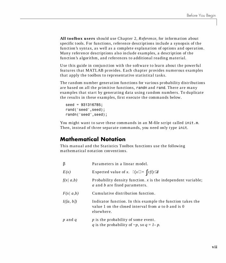
Mathematical NotationThis manual and the Statistics Toolbox functions use the followingmathematical notation conventions.
β Parameters in a linear model.
E(x) Expected value of x.
f(x|a,b) Probability density function. x is the independent variable;a and b are fixed parameters.
F(x|a,b) Cumulative distribution function.
I([a, b]) Indicator function. In this example the function takes thevalue 1 on the closed interval from a to b and is 0elsewhere.
p and q p is the probability of some event.q is the probability of ~p, so q = 1– p.
E x( ) tf t( ) td∫=
vii
Preface
viii
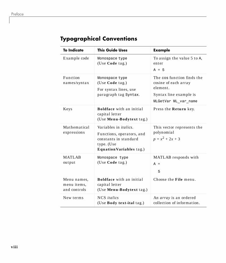
Typographical Conventions
To Indicate This Guide Uses Example
Example code Monospace type(Use Code tag.)
To assign the value 5 to A,enter
A = 5
Functionnames/syntax
Monospace type(Use Code tag.)
For syntax lines, useparagraph tag Syntax.
The cos function finds thecosine of each arrayelement.
Syntax line example is
MLGetVar ML_var_name
Keys Boldface with an initialcapital letter(Use Menu-Bodytext tag.)
Press the Return key.
Mathematicalexpressions
Variables in italics.
Functions, operators, andconstants in standardtype. (UseEquationVariables tag.)
This vector represents thepolynomial
p = x2 + 2x + 3
MATLABoutput
Monospace type(Use Code tag.)
MATLAB responds with
A =
5
Menu names,menu items,and controls
Boldface with an initialcapital letter(Use Menu-Bodytext tag.)
Choose the File menu.
New terms NCS italics(Use Body text-ital tag.)
An array is an orderedcollection of information.
Before You Begin
In addition, some words in our syntax lines are shown within single quotationmarks (sometimes double). These marks are a MATLAB requirement and mustbe typed. For example,
dir dirnamef = hex2num('s')
or
f ="pressure"
ix

Preface
x
Probability Distributions . . . . . . . . . . . . . . 1-5
Descriptive Statistics . . . . . . . . . . . . . . . . 1-42
Cluster Analysis . . . . . . . . . . . . . . . . . . 1-50
Linear Models . . . . . . . . . . . . . . . . . . . 1-65
Nonlinear Regression Models . . . . . . . . . . . . 1-79
Hypothesis Tests . . . . . . . . . . . . . . . . . . 1-85
Multivariate Statistics . . . . . . . . . . . . . . . 1-91
Statistical Plots . . . . . . . . . . . . . . . . . 1-103
Statistical Process Control (SPC) . . . . . . . . . 1-110
Design of Experiments (DOE) . . . . . . . . . . . 1-115
Demos . . . . . . . . . . . . . . . . . . . . . . 1-125
References . . . . . . . . . . . . . . . . . . . . 1-134
1
Tutorial
Introduction . . . . . . . . . . . . . . . . . . . . 1-2
1 Tutorial
1-2
IntroductionThe Statistics Toolbox, for use with MATLAB, supplies basic statisticscapability on the level of a first course in engineering or scientific statistics.The statistics functions it provides are building blocks suitable for use insideother analytical tools.
Primary Topic AreasThe Statistics Toolbox has more than 200 M-files, supporting work in thetopical areas below:
• Probability distributions
• Descriptive statistics
• Cluster Analysis
• Linear models
• Nonlinear models
• Hypothesis tests
• Multivariate statistics
• Statistical plots
• Statistical Process Control
• Design of Experiments
Probability DistributionsThe Statistics Toolbox supports 20 probability distributions. For eachdistribution there are five associated functions. They are:
• Probability density function (pdf)
• Cumulative distribution function (cdf)
• Inverse of the cumulative distribution function
• Random number generator
• Mean and variance as a function of the parameters
For data driven distributions (beta, binomial, exponential, gamma, normal,Poisson, uniform and Weibull), the Statistics Toolbox has functions forcomputing parameter estimates and confidence intervals.

Introduction
Descriptive StatisticsThe Statistics Toolbox provides functions for describing the features of a datasample. These descriptive statistics include measures of location and spread,percentile estimates and functions for dealing with data having missingvalues.
Cluster AnalysisThe Statistics Toolbox provides functions that allow you to divide a set ofobjects into subgroups, each having members that are as much alike aspossible. This process is called cluster analysis.
Linear ModelsIn the area of linear models the Statistics Toolbox supports one-way andtwo-way analysis of variance (ANOVA), multiple linear regression, stepwiseregression, response surface prediction, and ridge regression.
Nonlinear ModelsFor nonlinear models there are functions for parameter estimation, interactiveprediction and visualization of multidimensional nonlinear fits, and confidenceintervals for parameters and predicted values.
Hypothesis TestsThere are also functions that do the most common tests of hypothesis – t-testsand Z-tests.
Multivariate StatisticsThe Statistics Toolbox supports methods in Multivariate Statistics, includingPrincipal Components Analysis and Linear Discriminant Analysis.
Statistical PlotsThe Statistics Toolbox adds box plots, normal probability plots, Weibullprobability plots, control charts, and quantile-quantile plots to the arsenal ofgraphs in MATLAB. There is also extended support for polynomial curve fittingand prediction.
1-3
1 Tutorial
1-4
Statistical Process Control (SPC)For SPC there are functions for plotting common control charts and performingprocess capability studies.
Design of Experiments (DOE)The Statistics Toolbox supports both factorial and D-optimal design. There arefunctions for generating designs, augmenting designs and optimally assigningunits with fixed covariates.
Probability Distributions
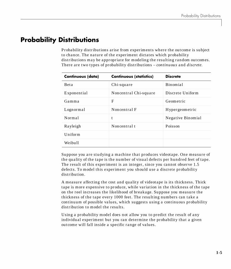
Probability DistributionsProbability distributions arise from experiments where the outcome is subjectto chance. The nature of the experiment dictates which probabilitydistributions may be appropriate for modeling the resulting random outcomes.There are two types of probability distributions – continuous and discrete.
Suppose you are studying a machine that produces videotape. One measure ofthe quality of the tape is the number of visual defects per hundred feet of tape.The result of this experiment is an integer, since you cannot observe 1.5defects. To model this experiment you should use a discrete probabilitydistribution.
A measure affecting the cost and quality of videotape is its thickness. Thicktape is more expensive to produce, while variation in the thickness of the tapeon the reel increases the likelihood of breakage. Suppose you measure thethickness of the tape every 1000 feet. The resulting numbers can take acontinuum of possible values, which suggests using a continuous probabilitydistribution to model the results.
Using a probability model does not allow you to predict the result of anyindividual experiment but you can determine the probability that a givenoutcome will fall inside a specific range of values.
Continuous (data) Continuous (statistics) Discrete
Beta Chi-square Binomial
Exponential Noncentral Chi-square Discrete Uniform
Gamma F Geometric
Lognormal Noncentral F Hypergeometric
Normal t Negative Binomial
Rayleigh Noncentral t Poisson
Uniform
Weibull
1-5
1 Tutorial
1-6
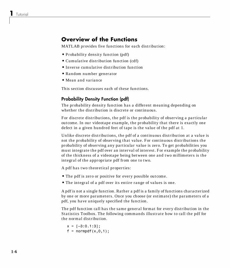
Overview of the FunctionsMATLAB provides five functions for each distribution:
• Probability density function (pdf)
• Cumulative distribution function (cdf)
• Inverse cumulative distribution function
• Random number generator
• Mean and variance
This section discusses each of these functions.
Probability Density Function (pdf)The probability density function has a different meaning depending onwhether the distribution is discrete or continuous.
For discrete distributions, the pdf is the probability of observing a particularoutcome. In our videotape example, the probability that there is exactly onedefect in a given hundred feet of tape is the value of the pdf at 1.
Unlike discrete distributions, the pdf of a continuous distribution at a value isnot the probability of observing that value. For continuous distributions theprobability of observing any particular value is zero. To get probabilities youmust integrate the pdf over an interval of interest. For example the probabilityof the thickness of a videotape being between one and two millimeters is theintegral of the appropriate pdf from one to two.
A pdf has two theoretical properties:
• The pdf is zero or positive for every possible outcome.
• The integral of a pdf over its entire range of values is one.
A pdf is not a single function. Rather a pdf is a family of functions characterizedby one or more parameters. Once you choose (or estimate) the parameters of apdf, you have uniquely specified the function.
The pdf function call has the same general format for every distribution in theStatistics Toolbox. The following commands illustrate how to call the pdf forthe normal distribution.
x = [–3:0.1:3];f = normpdf(x,0,1);

Probability Distributions
The variable f contains the density of the normal pdf with parameters 0 and 1at the values in x. The first input argument of every pdf is the set of values forwhich you want to evaluate the density. Other arguments contain as manyparameters as are necessary to define the distribution uniquely. The normaldistribution requires two parameters, a location parameter (the mean, µ) anda scale parameter (the standard deviation, σ).
Cumulative Distribution Function (cdf)If f is a probability density function, the associated cumulative distributionfunction F is
The cdf of a value x, F(x), is the probability of observing any outcome less thanor equal to x.
A cdf has two theoretical properties:
• The cdf ranges from 0 to 1.
• If y > x, then the cdf of y is greater than or equal to the cdf of x.
The cdf function call has the same general format for every distribution in theStatistics Toolbox. The following commands illustrate how to call the cdf for thenormal distribution:
x = [–3:0.1:3];p = normcdf(x,0,1);
The variable p contains the probabilities associated with the normal cdf withparameters 0 and 1 at the values in x. The first input argument of every cdf isthe set of values for which you want to evaluate the probability. Otherarguments contain as many parameters as are necessary to define thedistribution uniquely.
Inverse Cumulative Distribution FunctionThe inverse cumulative distribution function returns critical values forhypothesis testing given significance probabilities. To understand the
F x( ) P X x≤( ) f t( ) td∞–
x
∫= =
1-7
1 Tutorial
1-8
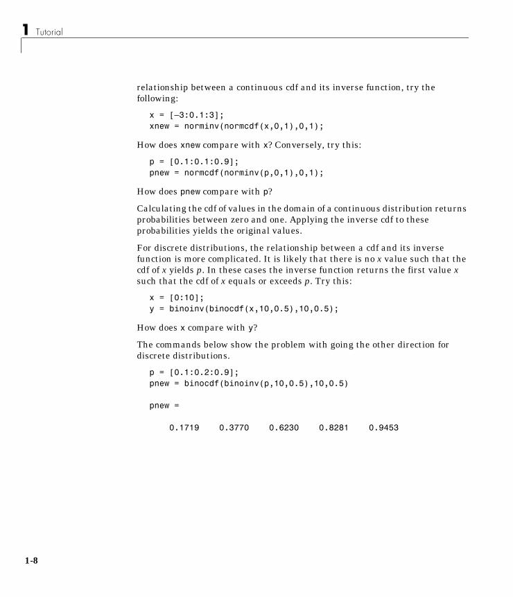
relationship between a continuous cdf and its inverse function, try thefollowing:
x = [–3:0.1:3];xnew = norminv(normcdf(x,0,1),0,1);
How does xnew compare with x? Conversely, try this:
p = [0.1:0.1:0.9];pnew = normcdf(norminv(p,0,1),0,1);
How does pnew compare with p?
Calculating the cdf of values in the domain of a continuous distribution returnsprobabilities between zero and one. Applying the inverse cdf to theseprobabilities yields the original values.
For discrete distributions, the relationship between a cdf and its inversefunction is more complicated. It is likely that there is no x value such that thecdf of x yields p. In these cases the inverse function returns the first value xsuch that the cdf of x equals or exceeds p. Try this:
x = [0:10];y = binoinv(binocdf(x,10,0.5),10,0.5);
How does x compare with y?
The commands below show the problem with going the other direction fordiscrete distributions.
p = [0.1:0.2:0.9];pnew = binocdf(binoinv(p,10,0.5),10,0.5)
pnew =
0.1719 0.3770 0.6230 0.8281 0.9453
Probability Distributions
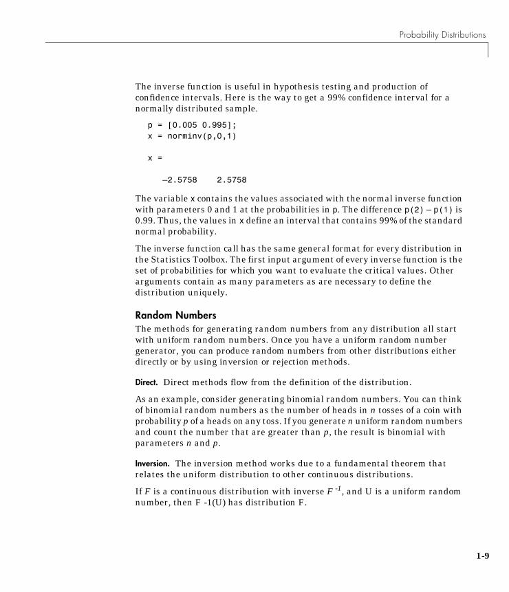
The inverse function is useful in hypothesis testing and production ofconfidence intervals. Here is the way to get a 99% confidence interval for anormally distributed sample.
p = [0.005 0.995];x = norminv(p,0,1)
x =
–2.5758 2.5758
The variable x contains the values associated with the normal inverse functionwith parameters 0 and 1 at the probabilities in p. The difference p(2) – p(1) is0.99. Thus, the values in x define an interval that contains 99% of the standardnormal probability.
The inverse function call has the same general format for every distribution inthe Statistics Toolbox. The first input argument of every inverse function is theset of probabilities for which you want to evaluate the critical values. Otherarguments contain as many parameters as are necessary to define thedistribution uniquely.
Random NumbersThe methods for generating random numbers from any distribution all startwith uniform random numbers. Once you have a uniform random numbergenerator, you can produce random numbers from other distributions eitherdirectly or by using inversion or rejection methods.
Direct. Direct methods flow from the definition of the distribution.
As an example, consider generating binomial random numbers. You can thinkof binomial random numbers as the number of heads in n tosses of a coin withprobability p of a heads on any toss. If you generate n uniform random numbersand count the number that are greater than p, the result is binomial withparameters n and p.
Inversion. The inversion method works due to a fundamental theorem thatrelates the uniform distribution to other continuous distributions.
If F is a continuous distribution with inverse F -1, and U is a uniform randomnumber, then F -1(U) has distribution F.
1-9
1 Tutorial
1-1
So, you can generate a random number from a distribution by applying theinverse function for that distribution to a uniform random number.Unfortunately, this approach is usually not the most efficient.
Rejection. The functional form of some distributions makes it difficult or timeconsuming to generate random numbers using direct or inversion methods.Rejection methods can sometimes provide an elegant solution in these cases.
Suppose you want to generate random numbers from a distribution with pdf f.To use rejection methods you must first find another density, g, and a constant,c, so that the inequality below holds.
You then generate the random numbers you want using the following steps:
1 Generate a random number x from distribution G with density g.
2 Form the ratio
3 Generate a uniform random number u.
4 If the product of u and r is less than one, return x.
5 Otherwise repeat steps one to three.
For efficiency you need a cheap method for generating random numbers fromG and the scalar, c, should be small. The expected number of iterations is c.
Syntax for Random Number Functions. You can generate random numbers fromeach distribution. This function provides a single random number or a matrixof random numbers, depending on the arguments you specify in the functioncall.
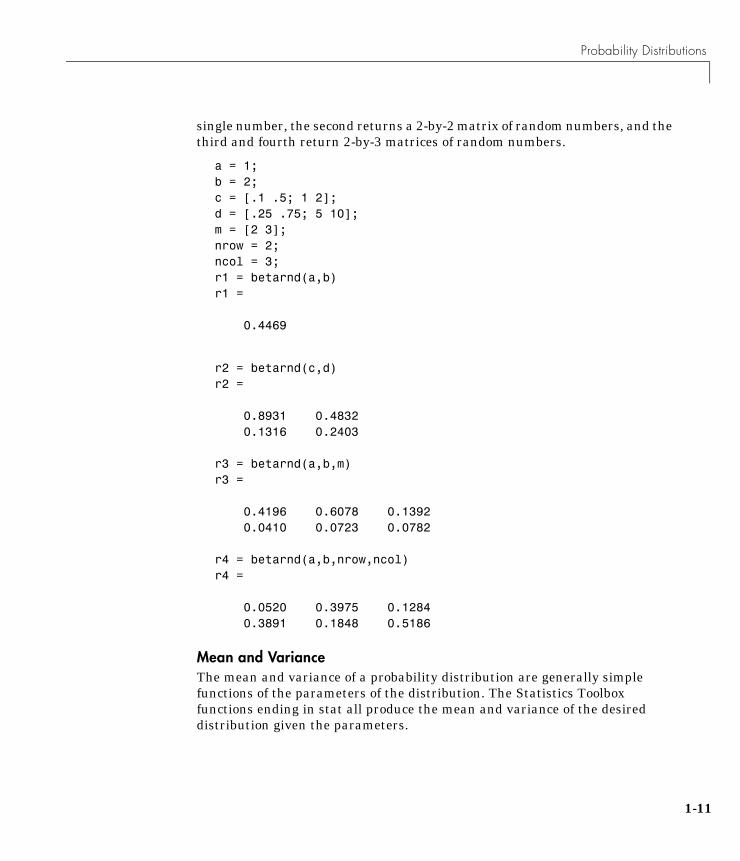
For example, here is the way to generate random numbers from the betadistribution. Four statements obtain random numbers: the first returns a
f x( ) cg x( ) x∀≤
rcg x( )f x( )--------------=
0
Probability Distributions
single number, the second returns a 2-by-2 matrix of random numbers, and thethird and fourth return 2-by-3 matrices of random numbers.
a = 1;b = 2;c = [.1 .5; 1 2];d = [.25 .75; 5 10];m = [2 3];nrow = 2;ncol = 3;r1 = betarnd(a,b)r1 =
0.4469
r2 = betarnd(c,d)r2 =
0.8931 0.4832 0.1316 0.2403
r3 = betarnd(a,b,m)r3 =
0.4196 0.6078 0.1392 0.0410 0.0723 0.0782
r4 = betarnd(a,b,nrow,ncol)r4 =
0.0520 0.3975 0.1284 0.3891 0.1848 0.5186
Mean and VarianceThe mean and variance of a probability distribution are generally simplefunctions of the parameters of the distribution. The Statistics Toolboxfunctions ending in stat all produce the mean and variance of the desireddistribution given the parameters.
1-11
1 Tutorial
1-1
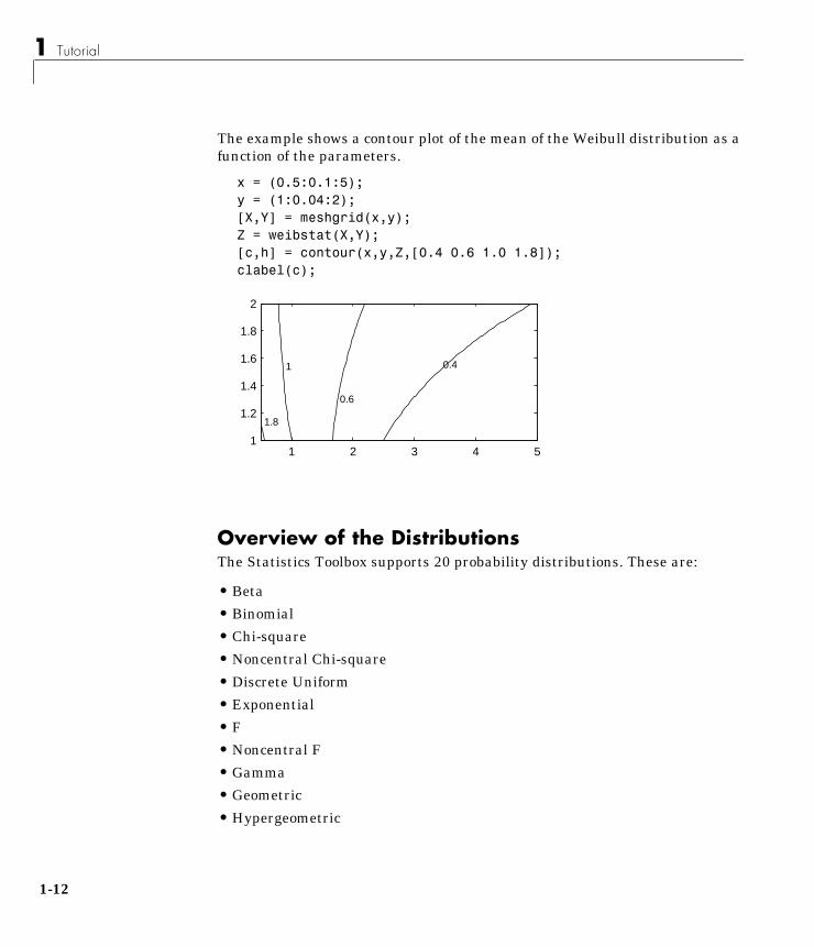
The example shows a contour plot of the mean of the Weibull distribution as afunction of the parameters.
x = (0.5:0.1:5);y = (1:0.04:2);[X,Y] = meshgrid(x,y);Z = weibstat(X,Y);[c,h] = contour(x,y,Z,[0.4 0.6 1.0 1.8]);clabel(c);
Overview of the DistributionsThe Statistics Toolbox supports 20 probability distributions. These are:
• Beta
• Binomial
• Chi-square
• Noncentral Chi-square
• Discrete Uniform
• Exponential
• F
• Noncentral F
• Gamma
• Geometric
• Hypergeometric
1 2 3 4 51
1.2
1.4
1.6
1.8
2
0.4
0.6
1
1.8
2
Probability Distributions
• Lognormal
• Negative Binomial
• Normal
• Poisson
• Rayleigh
• Student’s t
• Noncentral t
• Uniform
• Weibull
This section gives a short introduction to each distribution.
Beta Distribution
Background. The beta distribution describes a family of curves that are uniquein that they are nonzero only on the interval [0 1]. A more general version ofthe function assigns parameters to the end-points of the interval.
The beta cdf is the same as the incomplete beta function.
The beta distribution has a functional relationship with the t distribution. If Yis an observation from Student’s t distribution with ν degrees of freedom thenthe following transformation generates X, which is beta distributed:
if: then
The Statistics Toolbox uses this relationship to compute values of the t cdf andinverse function as well as generating t distributed random numbers.
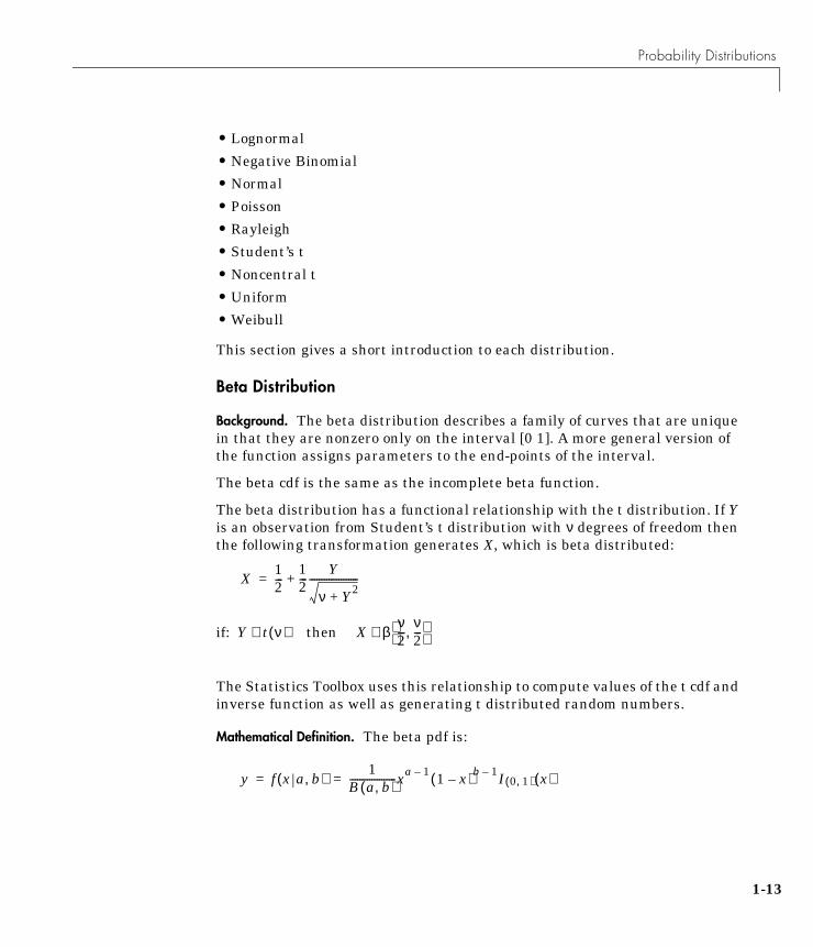
Mathematical Definition. The beta pdf is:
X12---
12---
Y
ν Y2+
--------------------+=
Y t ν( )∼ X βν2---
ν2---,
∼
y f x a b,( )1
B a b,( )-------------------xa 1– 1 x–( )b 1– I 0 1,( ) x( )= =
1-13
1 Tutorial
1-1
Parameter Estimation. Suppose you are collecting data that has hard lower andupper bounds of zero and one respectively. Parameter estimation is the processof determining the parameters of the beta distribution that fit this data best insome sense.
One popular criterion of goodness is to maximize the likelihood function. Thelikelihood has the same form as the beta pdf. But for the pdf, the parametersare known constants and the variable is x. The likelihood function reverses theroles of the variables. Here, the sample values (the xs) are already observed. Sothey are the fixed constants. The variables are the unknown parameters.Maximum likelihood estimation (MLE) involves calculating the values of theparameters that give the highest likelihood given the particular set of data.
The function betafit returns the MLEs and confidence intervals for theparameters of the beta distribution. Here is an example using random numbersfrom the beta distribution with a = 5 and b = 0.2.
r = betarnd(5,0.2,100,1);[phat, pci] = betafit(r)
phat =
4.5330 0.2301
pci =
2.8051 0.1771 6.2610 0.2832
The MLE for the parameter, a is 4.5330 compared to the true value of 5. The95% confidence interval for a goes from 2.8051 to 6.2610, which includes thetrue value.
Similarly the MLE for the parameter, b is 0.2301 compared to the true value of0.2. The 95% confidence interval for b goes from 0.1771 to 0.2832, which alsoincludes the true value.
Of course in this made-up example we know the “true value.” Inexperimentation we do not.
4
Probability Distributions
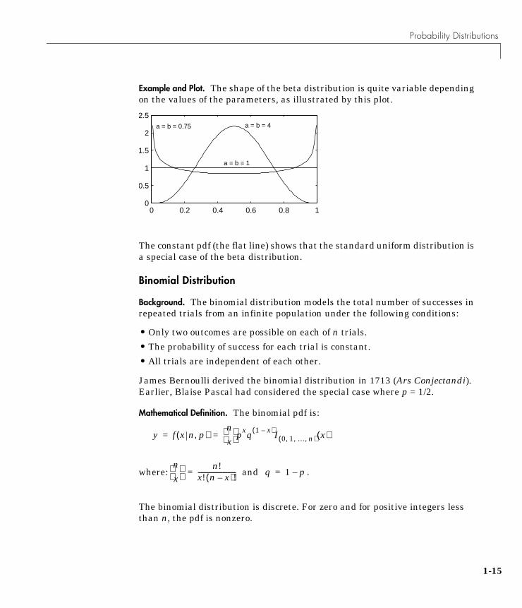
Example and Plot. The shape of the beta distribution is quite variable dependingon the values of the parameters, as illustrated by this plot.
The constant pdf (the flat line) shows that the standard uniform distribution isa special case of the beta distribution.
Binomial Distribution
Background. The binomial distribution models the total number of successes inrepeated trials from an infinite population under the following conditions:
• Only two outcomes are possible on each of n trials.
• The probability of success for each trial is constant.
• All trials are independent of each other.
James Bernoulli derived the binomial distribution in 1713 (Ars Conjectandi).Earlier, Blaise Pascal had considered the special case where p = 1/2.
Mathematical Definition. The binomial pdf is:
where: and .
The binomial distribution is discrete. For zero and for positive integers lessthan n, the pdf is nonzero.
0 0.2 0.4 0.6 0.8 10
0.5
1
1.5
2
2.5
a = b = 1
a = b = 4 a = b = 0.75
y f x n p,( )nx
pxq 1 x–( )I 0 1 … n, , ,( ) x( )= =
nx
n!x! n x–( )!------------------------= q 1 p–=
1-15
1 Tutorial
1-1
Parameter Estimation. Suppose you are collecting data from a widgetmanufacturing process, and you record the number of widgets withinspecification in each batch of 100. You might be interested in the probabilitythat an individual widget is within specification. Parameter estimation is theprocess of determining the parameter, p, of the binomial distribution that fitsthis data best in some sense.
One popular criterion of goodness is to maximize the likelihood function. Thelikelihood has the same form as the binomial pdf above. But for the pdf, theparameters (n and p) are known constants and the variable is x. The likelihoodfunction reverses the roles of the variables. Here, the sample values (the xs) arealready observed. So they are the fixed constants. The variables are theunknown parameters. MLE involves calculating the value of p that give thehighest likelihood given the particular set of data.
The function binofit returns the MLEs and confidence intervals for theparameters of the binomial distribution. Here is an example using randomnumbers from the binomial distribution with n = 100 and p = 0.9.
r = binornd(100,0.9)
r =
88
[phat, pci] = binofit(r,100)
phat =
0.8800
pci =
0.7998 0.9364
The MLE for the parameter, p is 0.8800 compared to the true value of 0.9. The95% confidence interval for p goes from 0.7998 to 0.9364, which includes thetrue value.
Of course in this made-up example we know the “true value” of p.
6

Probability Distributions
Example and Plot. The following commands generate a plot of the binomial pdffor n = 10 and p = 1/2.
x = 0:10;y = binopdf(x,10,0.5);plot(x,y,'+')
Chi-Square (χ2) Distribution
Background. The χ2 distribution is a special case of the gamma distributionwhere b = 2, in the equation for gamma distribution below.
The χ2 distribution gets special attention because of its importance in normalsampling theory. If a set of n observations are normally distributed withvariance σ2, and s2 is the sample standard deviation, then:
0 2 4 6 8 100
0.05
0.1
0.15
0.2
0.25
y f x a b,( )1
baΓ a( )------------------xa 1– e
xb---–
= =
n 1–( )s2
σ2----------------------- χ2 n 1–( )∼
1-17
1 Tutorial
1-1
The Statistics Toolbox uses the above relationship to calculate confidenceintervals for the estimate of the normal parameter σ2 in the function normfit.
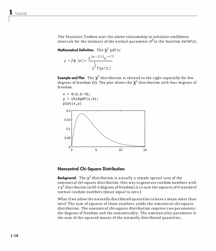
Mathematical Definition. The χ2 pdf is:
Example and Plot. The χ2 distribution is skewed to the right especially for fewdegrees of freedom (ν). The plot shows the χ2 distribution with four degrees offreedom.
x = 0:0.2:15;y = chi2pdf(x,4);plot(x,y)
Noncentral Chi-Square Distribution
Background. The χ2 distribution is actually a simple special case of thenoncentral chi-square distribution. One way to generate random numbers witha χ2 distribution (with ν degrees of freedom) is to sum the squares of ν standardnormal random numbers (mean equal to zero.)
What if we allow the normally distributed quantities to have a mean other thanzero? The sum of squares of these numbers yields the noncentral chi-squaredistribution. The noncentral chi-square distribution requires two parameters:the degrees of freedom and the noncentrality. The noncentrality parameter isthe sum of the squared means of the normally distributed quantities.
y f x ν( ) x ν 2–( ) 2⁄ e x– 2⁄
2
v2--- Γ ν 2⁄( )
-------------------------------------= =
0 5 10 150
0.05
0.1
0.15
0.2
8
Probability Distributions
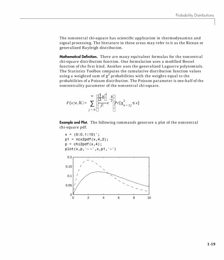
The noncentral chi-square has scientific application in thermodynamics andsignal processing. The literature in these areas may refer to it as the Ricean orgeneralized Rayleigh distribution.
Mathematical Definition. There are many equivalent formulas for the noncentralchi-square distribution function. One formulation uses a modified Besselfunction of the first kind. Another uses the generalized Laguerre polynomials.The Statistics Toolbox computes the cumulative distribution function valuesusing a weighted sum of χ2 probabilities with the weights equal to theprobabilities of a Poisson distribution. The Poisson parameter is one-half of thenoncentrality parameter of the noncentral chi-square.
Example and Plot. The following commands generate a plot of the noncentralchi-square pdf.
x = (0:0.1:10)';p1 = ncx2pdf(x,4,2);p = chi2pdf(x,4);plot(x,p,'– –',x,p1,'–')
F x ν δ,( )
12---δ
j
j!-------------e
δ2---–
Pr χν 2 j+
2 x≤[ ]
j 0=
∞
∑=
0 2 4 6 8 100
0.05
0.1
0.15
0.2
1-19
1 Tutorial
1-2
Discrete Uniform Distribution
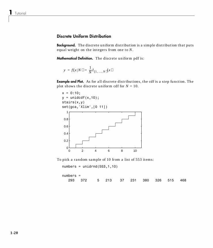
Background. The discrete uniform distribution is a simple distribution that putsequal weight on the integers from one to N.
Mathematical Definition. The discrete uniform pdf is:
Example and Plot. As for all discrete distributions, the cdf is a step function. Theplot shows the discrete uniform cdf for N = 10.
x = 0:10;y = unidcdf(x,10);stairs(x,y)set(gca,'Xlim',[0 11])
To pick a random sample of 10 from a list of 553 items:
numbers = unidrnd(553,1,10)
numbers =293 372 5 213 37 231 380 326 515 468
y f x N( )1N----I 1 … N, ,( ) x( )= =
0 2 4 6 8 100
0.2
0.4
0.6
0.8
1
0
Probability Distributions
Exponential Distribution
Background. Like the chi-square, the exponential distribution is a special caseof the gamma distribution (obtained by setting a = 1 in the equation below.)
The exponential distribution is special because of its utility in modeling eventsthat occur randomly over time. The main application area is in studies oflifetimes.
Mathematical Definition. The exponential pdf is:
Parameter Estimation. Suppose you are stress testing light bulbs and collectingdata on their lifetimes. You assume that these lifetimes follow an exponentialdistribution. You want to know how long you can expect the average light bulbto last. Parameter estimation is the process of determining the parameters ofthe exponential distribution that fit this data best in some sense.
One popular criterion of goodness is to maximize the likelihood function. Thelikelihood has the same form as the beta pdf on the previous page. But for thepdf, the parameters are known constants and the variable is x. The likelihoodfunction reverses the roles of the variables. Here, the sample values (the xs) arealready observed. So they are the fixed constants. The variables are theunknown parameters. MLE involves calculating the values of the parametersthat give the highest likelihood given the particular set of data.
y f x a b,( )1
baΓ a( )------------------xa 1– e
xb---–
= =
y f x µ( )1µ---e
xµ---–
= =
1-21
1 Tutorial
1-2
The function expfit returns the MLEs and confidence intervals for theparameters of the exponential distribution. Here is an example using randomnumbers from the exponential distribution with µ = 700.
lifetimes = exprnd(700,100,1);[muhat, muci] = expfit(lifetimes)muhat = 672.8207
muci =
547.4338 810.9437
The MLE for the parameter, µ is 672 compared to the true value of 700. The95% confidence interval for µ goes from 547 to 811, which includes the truevalue.
In our life tests we do not know the true value of µ so it is nice to have aconfidence interval on the parameter to give a range of likely values.
Example and Plot. For exponentially distributed lifetimes, the probability thatan item will survive an extra unit of time is independent of the current age ofthe item. The example shows a specific case of this special property.
l = 10:10:60;lpd = l+0.1;deltap = (expcdf(lpd,50)–expcdf(l,50))./(1–expcdf(l,50))
deltap =
0.0020 0.0020 0.0020 0.0020 0.0020 0.0020
2

Probability Distributions
The plot shows the exponential pdf with its parameter (and mean), lambda, setto two.
x = 0:0.1:10;y = exppdf(x,2);plot(x,y)
F Distribution
Background. The F distribution has a natural relationship with the chi-squaredistribution. If χ1 and χ2 are both chi-square with ν1 and ν2 degrees of freedomrespectively, then the statistic, F is F distributed.
The two parameters, ν1 and ν2, are the numerator and denominator degrees offreedom. That is, ν1 and ν2 are the number of independent pieces informationused to calculate χ1 and χ2 respectively.
Mathematical Definition. The pdf for the F distribution is:
0 2 4 6 8 100
0.1
0.2
0.3
0.4
0.5
F ν1 ν2,( )
χ1ν1------
χ2ν2------
------=
y f x ν1 ν2,( )Γ
ν1 ν2+( )2-----------------------
Γν12------
Γν22------
--------------------------------
ν1ν2------
ν1
2----- xν1 2–
2--------------
1ν1ν2------
x+
ν1 ν2+2-----------------
-------------------------------------------= =
1-23
1 Tutorial
1-2
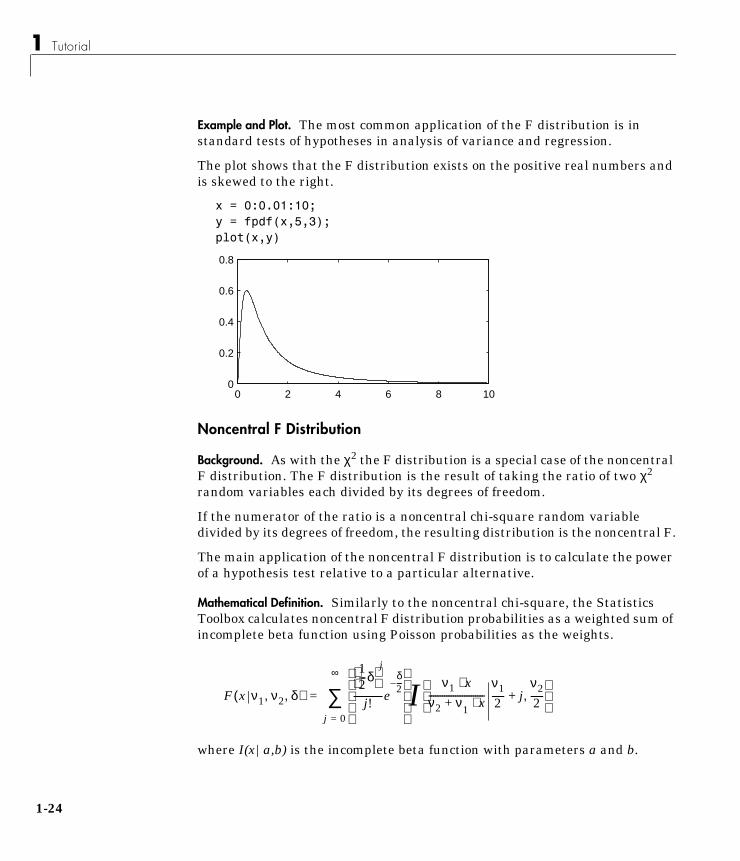
Example and Plot. The most common application of the F distribution is instandard tests of hypotheses in analysis of variance and regression.
The plot shows that the F distribution exists on the positive real numbers andis skewed to the right.
x = 0:0.01:10;y = fpdf(x,5,3);plot(x,y)
Noncentral F Distribution
Background. As with the χ2 the F distribution is a special case of the noncentralF distribution. The F distribution is the result of taking the ratio of two χ2
random variables each divided by its degrees of freedom.
If the numerator of the ratio is a noncentral chi-square random variabledivided by its degrees of freedom, the resulting distribution is the noncentral F.
The main application of the noncentral F distribution is to calculate the powerof a hypothesis test relative to a particular alternative.
Mathematical Definition. Similarly to the noncentral chi-square, the StatisticsToolbox calculates noncentral F distribution probabilities as a weighted sum ofincomplete beta function using Poisson probabilities as the weights.
where I(x|a,b) is the incomplete beta function with parameters a and b.
0 2 4 6 8 100
0.2
0.4
0.6
0.8
F x ν1 ν2 δ, ,( )
12---δ
j
j!-------------e
δ2---–
I ν1 x⋅ν2 ν+ 1 x⋅-------------------------
ν12------ j+
ν22------,
j 0=
∞
∑=
4
Probability Distributions
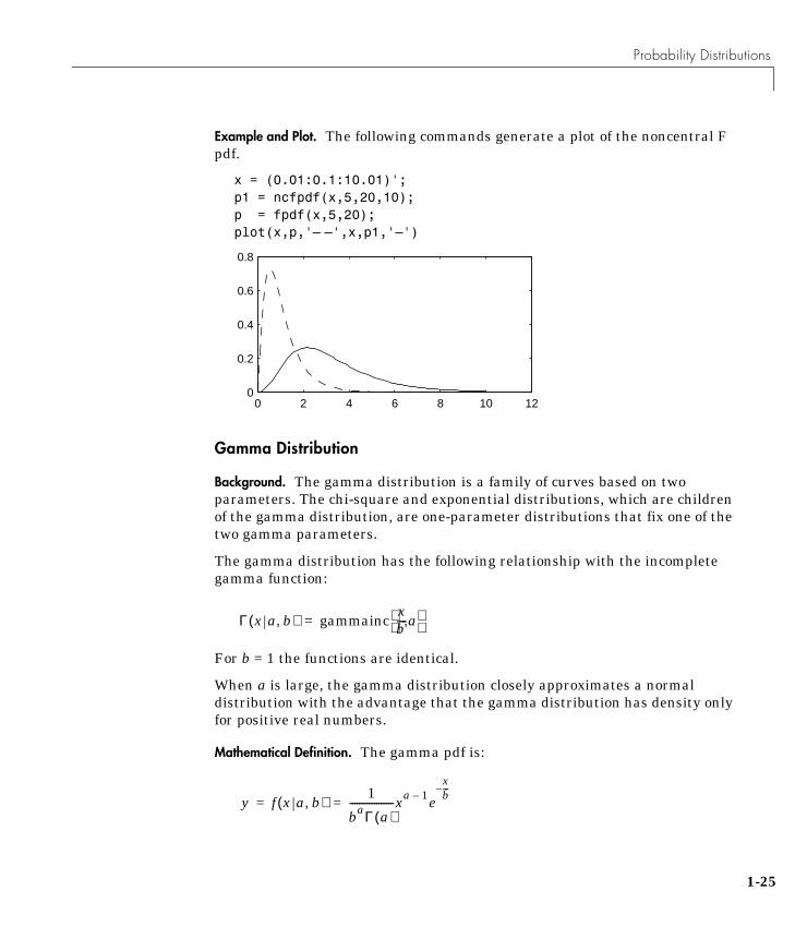
Example and Plot. The following commands generate a plot of the noncentral Fpdf.
x = (0.01:0.1:10.01)';p1 = ncfpdf(x,5,20,10);p = fpdf(x,5,20);plot(x,p,'– –',x,p1,'–')
Gamma Distribution
Background. The gamma distribution is a family of curves based on twoparameters. The chi-square and exponential distributions, which are childrenof the gamma distribution, are one-parameter distributions that fix one of thetwo gamma parameters.
The gamma distribution has the following relationship with the incompletegamma function:
For b = 1 the functions are identical.
When a is large, the gamma distribution closely approximates a normaldistribution with the advantage that the gamma distribution has density onlyfor positive real numbers.
Mathematical Definition. The gamma pdf is:
0 2 4 6 8 10 120
0.2
0.4
0.6
0.8
Γ x a b,( ) gammaincxb'----a
=
y f x a b,( )1
baΓ a( )------------------xa 1– e
xb---–
= =
1-25
1 Tutorial
1-2
Parameter Estimation. Suppose you are stress testing computer memory chips andcollecting data on their lifetimes. You assume that these lifetimes follow agamma distribution. You want to know how long you can expect the averagecomputer memory chip to last. Parameter estimation is the process ofdetermining the parameters of the gamma distribution that fit this data bestin some sense.
One popular criterion of goodness is to maximize the likelihood function. Thelikelihood has the same form as the gamma pdf above. But for the pdf, theparameters are known constants and the variable is x. The likelihood functionreverses the roles of the variables. Here, the sample values (the xs) are alreadyobserved. So they are the fixed constants. The variables are the unknownparameters. MLE involves calculating the values of the parameters that givethe highest likelihood given the particular set of data.
The function gamfit returns the MLEs and confidence intervals for theparameters of the gamma distribution. Here is an example using randomnumbers from the gamma distribution with a = 10 and b = 5.
lifetimes = gamrnd(10,5,100,1);[phat, pci] = gamfit(lifetimes)phat = 10.9821 4.7258
pci =
7.4001 3.1543 14.5640 6.2974
Note phat(1) = and phat(2) = . The MLE for the parameter, a is 10.98compared to the true value of 10. The 95% confidence interval for a goes from7.4 to 14.6, which includes the true value.
Similarly the MLE for the parameter, b is 4.7 compared to the true value of 5.The 95% confidence interval for b goes from 3.2 to 6.3, which also includes thetrue value.
In our life tests we do not know the true value of a and b so it is nice to have aconfidence interval on the parameters to give a range of likely values.
a b
6

Probability Distributions
Example and Plot. In the example the gamma pdf is plotted with the solid line.The normal pdf has a dashed line type.
x = gaminv((0.005:0.01:0.995),100,10);y = gampdf(x,100,10);y1 = normpdf(x,1000,100);plot(x,y,'–',x,y1,'–.')
Geometric Distribution
Background. The geometric distribution is discrete, existing only on thenonnegative integers. It is useful for modeling the runs of consecutivesuccesses (or failures) in repeated independent trials of a system.
The geometric distribution models the number of successes before one failurein an independent succession of tests where each test results in success orfailure.
Mathematical Definition. The geometric pdf is:
700 800 900 1000 1100 1200 13000
1
2
3
4
5x 10⁻³
y f x p( ) pqxI 0 1 K, ,( ) x( )= =
where q 1 p–=
1-27
1 Tutorial
1-2
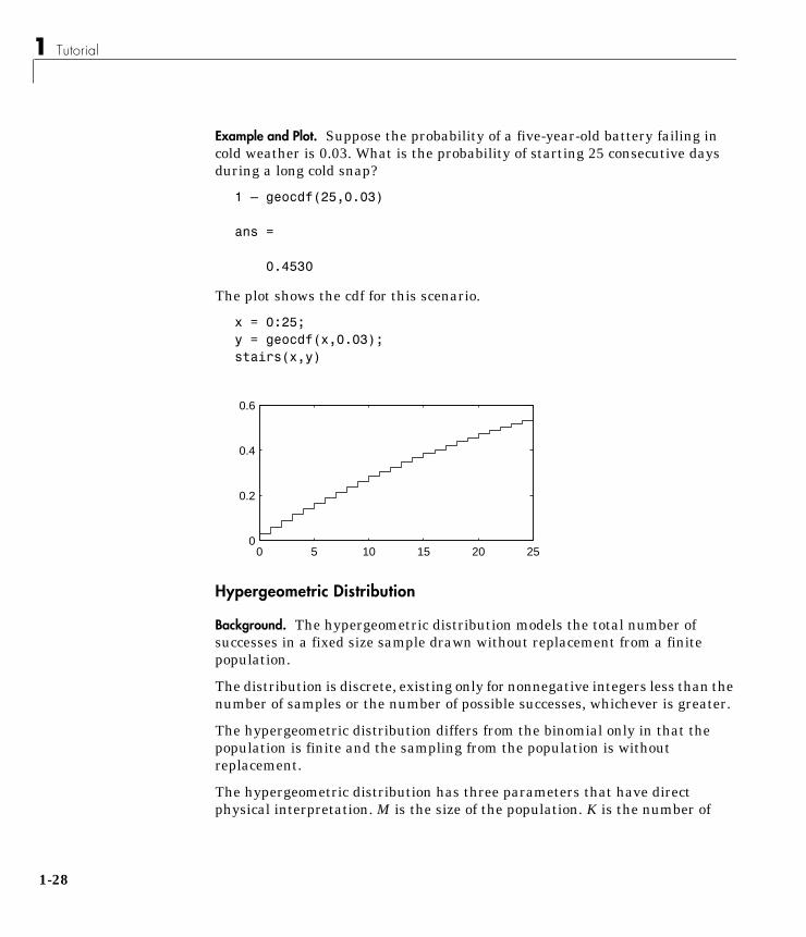
Example and Plot. Suppose the probability of a five-year-old battery failing incold weather is 0.03. What is the probability of starting 25 consecutive daysduring a long cold snap?
1 – geocdf(25,0.03)
ans =
0.4530
The plot shows the cdf for this scenario.
x = 0:25;y = geocdf(x,0.03);stairs(x,y)
Hypergeometric Distribution
Background. The hypergeometric distribution models the total number ofsuccesses in a fixed size sample drawn without replacement from a finitepopulation.
The distribution is discrete, existing only for nonnegative integers less than thenumber of samples or the number of possible successes, whichever is greater.
The hypergeometric distribution differs from the binomial only in that thepopulation is finite and the sampling from the population is withoutreplacement.
The hypergeometric distribution has three parameters that have directphysical interpretation. M is the size of the population. K is the number of
0 5 10 15 20 250
0.2
0.4
0.6
8

Probability Distributions
items with the desired characteristic in the population. n is the number ofsamples drawn. Sampling “without replacement” means that once a particularsample is chosen, it is removed from the relevant population for drawing thenext sample.
Mathematical Definition. The hypergeometric pdf is:
Example and Plot. The plot shows the cdf of an experiment taking 20 samplesfrom a group of 1000 where there are 50 items of the desired type.
x = 0:10;y = hygecdf(x,1000,50,20);stairs(x,y)
Lognormal Distribution
Background. The normal and lognormal distributions are closely related. If X isdistributed lognormal with parameters µ and σ2, then lnX is distributednormal with parameters µ and σ2.
The lognormal distribution is applicable when the quantity of interest must bepositive, since lnX exists only when the random variable X is positive.Economists often model the distribution of income using a lognormaldistribution.
y f x M K n, ,( )
Kx
M K–
n x–
Mn
------------------------------= =
0 2 4 6 8 100.2
0.4
0.6
0.8
1
1-29

1 Tutorial
1-3
Mathematical Definition. The lognormal pdf is:
Example and Plot. Suppose the income of a family of four in the United Statesfollows a lognormal distribution with µ = log(20,000) and σ2 = 1.0. Plot theincome density.
x = (10:1000:125010)';y=lognpdf(x,log(20000),1.0);plot(x,y)set(gca,'Xtick',[0 30000 60000 90000 120000 ])set(gca,'xticklabel',str2mat('0','$30,000','$60,000',...'$90,000','$120,000'))
Negative Binomial Distribution
Background. The geometric distribution is a special case of the negativebinomial distribution (also called the Pascal distribution). The geometricdistribution models the number of successes before one failure in anindependent succession of tests where each test results in success or failure.
In the negative binomial distribution the number of failures is a parameter ofthe distribution. The parameters are the probability of success, p, and thenumber of failures, r.
Mathematical Definition. The negative binomial pdf is
y f x µ σ,( ) 1xσ 2π------------------e
lnx µ–( )– 2
2σ2----------------------------
= =
0 $30,000 $60,000 $90,000 $120,0000
2
4x 10⁻⁵
0

Probability Distributions
where
Example and Plot. The following commands generate a plot of the negativebinomial pdf.
x = (0:10);y = nbinpdf(x,3,0.5);plot(x,y,'+')set(gca,'XLim',[–0.5,10.5])
Normal Distribution
Background. The normal distribution is a two parameter family of curves. Thefirst parameter, µ, is the mean. The second, σ, is the standard deviation. Thestandard normal distribution (written Φ(x)) sets µ to zero and σ to one.
Φ(x) is functionally related to the error function, erf.
The first use of the normal distribution was as a continuous approximation tothe binomial.
The usual justification for using the normal distribution for modeling is theCentral Limit Theorem which states (roughly) that the sum of independentsamples from any distribution with finite mean and variance converges to thenormal distribution as the sample size goes to infinity.
Mathematical Definition. The normal pdf is:
y f x r p,( ) r x 1–+x
prqxI 0 1 …, ,( ) x( )= =
q 1 p–=
0 2 4 6 8 100
0.05
0.1
0.15
0.2
erf x( ) 2Φ x 2( ) 1–=
1-31

1 Tutorial
1-3
Parameter Estimation. One of the first applications of the normal distribution indata analysis was modeling the height of school children. Suppose we want toestimate the mean, µ, and the variance, σ2, of all the 4th graders in the UnitedStates.
We have already introduced MLEs. Another desirable criterion in a statisticalestimator is unbiasedness. A statistic is unbiased if the expected value of thestatistic is equal to the parameter being estimated. MLEs are not alwaysunbiased. For any data sample, there may be more than one unbiasedestimator of the parameters of the parent distribution of the sample. Forinstance, every sample value is an unbiased estimate of the parameter µ of anormal distribution. The Minimum Variance Unbiased Estimator (MVUE) isthe statistic that has the minimum variance of all unbiased estimators of aparameter.
The MVUEs of the parameters, µ and σ2 for the normal distribution are thesample average and variance. The sample average is also the MLE for µ. Thereare two common textbook formulas for the variance.
They are:
Equation 1 is the maximum likelihood estimator for σ2, and equation 2 is theMVUE.
y f x µ σ,( )1
σ 2π---------------e
x µ–( )– 2
2σ2----------------------
= =
1) s2 1n---= xi x–( )
2
i 1=
n
∑
2) s2 1n 1–------------- xi x–( )
2
i 1=
n
∑
where x
=
xin----
n
∑=
2

Probability Distributions
The function normfit returns the MVUEs and confidence intervals for µ andσ2. Here is a playful example modeling the “heights” (inches) of a randomlychosen 4th grade class.
height = normrnd(50,2,30,1); % Simulate heights.[mu, s, muci, sci] = normfit(height)mu = 50.2025s = 1.7946muci = 49.5210 50.8841sci = 1.4292 2.4125
Example and Plot. The plot shows the “bell” curve of the standard normal pdfµ = 0, σ = 1.
Poisson Distribution
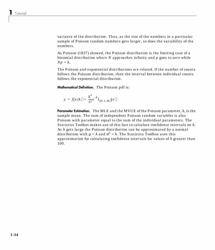
Background. The Poisson distribution is appropriate for applications thatinvolve counting the number of times a random event occurs in a given amountof time, distance, area, etc. Sample applications that involve Poissondistributions include the number of Geiger counter clicks per second, thenumber of people walking into a store in an hour, and the number of flaws per1000 feet of video tape.
The Poisson distribution is a one parameter discrete distribution that takesnonnegative integer values. The parameter, λ, is both the mean and the
-3 -2 -1 0 1 2 30
0.1
0.2
0.3
0.4
1-33
1 Tutorial
1-3
variance of the distribution. Thus, as the size of the numbers in a particularsample of Poisson random numbers gets larger, so does the variability of thenumbers.
As Poisson (1837) showed, the Poisson distribution is the limiting case of abinomial distribution where N approaches infinity and p goes to zero whileNp = λ.
The Poisson and exponential distributions are related. If the number of countsfollows the Poisson distribution, then the interval between individual countsfollows the exponential distribution.
Mathematical Definition. The Poisson pdf is:
Parameter Estimation. The MLE and the MVUE of the Poisson parameter, λ, is thesample mean. The sum of independent Poisson random variables is alsoPoisson with parameter equal to the sum of the individual parameters. TheStatistics Toolbox makes use of this fact to calculate confidence intervals on λ.As λ gets large the Poisson distribution can be approximated by a normaldistribution with µ = λ and σ2 = λ. The Statistics Toolbox uses thisapproximation for calculating confidence intervals for values of λ greater than100.
y f x λ( )λx
x!-----e λ– I 0 1 K, ,( ) x( )= =
4
Probability Distributions
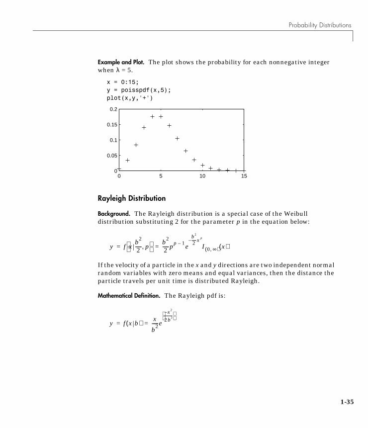
Example and Plot. The plot shows the probability for each nonnegative integerwhen λ = 5.
x = 0:15;y = poisspdf(x,5);plot(x,y,'+')
Rayleigh Distribution
Background. The Rayleigh distribution is a special case of the Weibulldistribution substituting 2 for the parameter p in the equation below:
If the velocity of a particle in the x and y directions are two independent normalrandom variables with zero means and equal variances, then the distance theparticle travels per unit time is distributed Rayleigh.
Mathematical Definition. The Rayleigh pdf is:
0 5 10 150
0.05
0.1
0.15
0.2
y f xb2
2------ p, b2
2------pp 1– e
b2
2-----x p–I 0 ∞,( ) x( )= =
y f x b( ) x
b2------e
x2–
2b2---------
= =
1-35
1 Tutorial
1-3
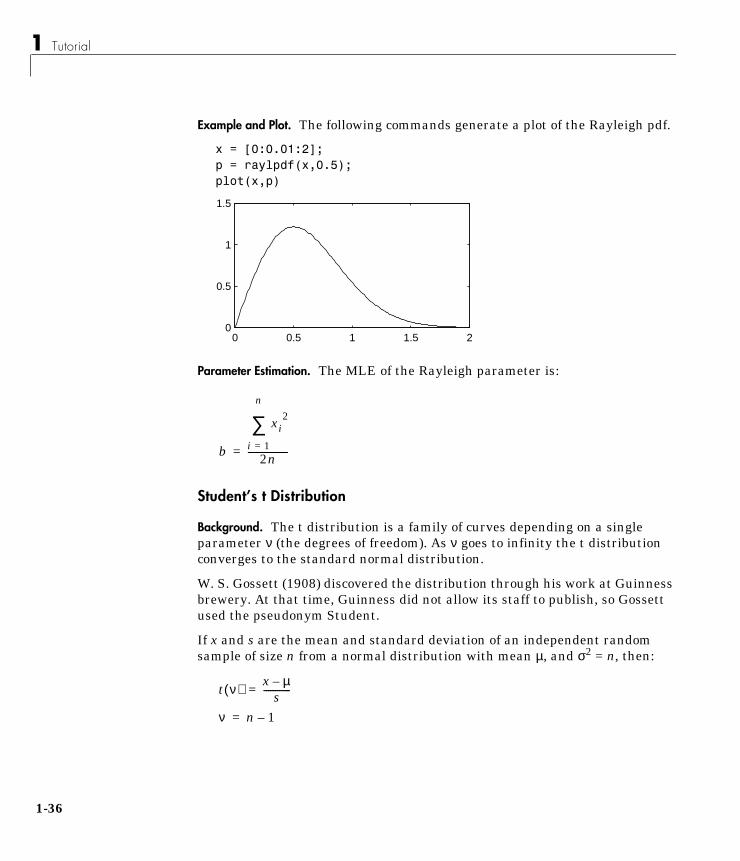
Example and Plot. The following commands generate a plot of the Rayleigh pdf.
x = [0:0.01:2];p = raylpdf(x,0.5);plot(x,p)
Parameter Estimation. The MLE of the Rayleigh parameter is:
Student’s t Distribution
Background. The t distribution is a family of curves depending on a singleparameter ν (the degrees of freedom). As ν goes to infinity the t distributionconverges to the standard normal distribution.
W. S. Gossett (1908) discovered the distribution through his work at Guinnessbrewery. At that time, Guinness did not allow its staff to publish, so Gossettused the pseudonym Student.
If x and s are the mean and standard deviation of an independent randomsample of size n from a normal distribution with mean µ, and σ2 = n, then:
0 0.5 1 1.5 20
0.5
1
1.5
b
xi2
i 1=
n
∑2n------------------=
t ν( ) x µ–s------------=
ν n 1–=
6
Probability Distributions
Mathematical Definition. Student’s t pdf is:
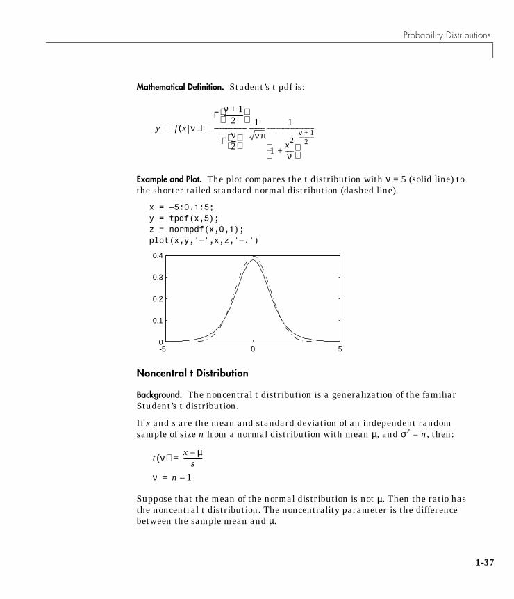
Example and Plot. The plot compares the t distribution with ν = 5 (solid line) tothe shorter tailed standard normal distribution (dashed line).
x = –5:0.1:5;y = tpdf(x,5);z = normpdf(x,0,1);plot(x,y,'–',x,z,'–.')
Noncentral t Distribution
Background. The noncentral t distribution is a generalization of the familiarStudent’s t distribution.
If x and s are the mean and standard deviation of an independent randomsample of size n from a normal distribution with mean µ, and σ2 = n, then:
Suppose that the mean of the normal distribution is not µ. Then the ratio hasthe noncentral t distribution. The noncentrality parameter is the differencebetween the sample mean and µ.
y f x ν( )Γ
ν 1+2------------
Γν2---
---------------------
1νπ
----------1
1x2
ν-----+
ν 1+2------------
-------------------------------= =
-5 0 50
0.1
0.2
0.3
0.4
t ν( ) x µ–s------------=
ν n 1–=
1-37
1 Tutorial
1-3
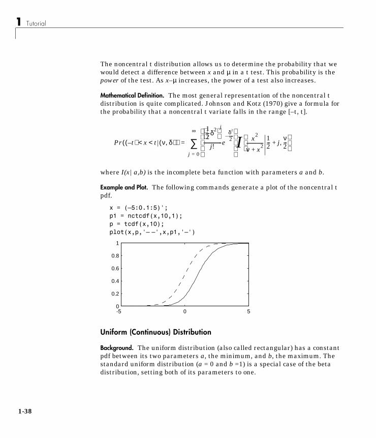
The noncentral t distribution allows us to determine the probability that wewould detect a difference between x and µ in a t test. This probability is thepower of the test. As x–µ increases, the power of a test also increases.
Mathematical Definition. The most general representation of the noncentral tdistribution is quite complicated. Johnson and Kotz (1970) give a formula forthe probability that a noncentral t variate falls in the range [–t, t].
where I(x|a,b) is the incomplete beta function with parameters a and b.
Example and Plot. The following commands generate a plot of the noncentral tpdf.
x = (–5:0.1:5)';p1 = nctcdf(x,10,1);p = tcdf(x,10);plot(x,p,'– –',x,p1,'–')
Uniform (Continuous) Distribution
Background. The uniform distribution (also called rectangular) has a constantpdf between its two parameters a, the minimum, and b, the maximum. Thestandard uniform distribution (a = 0 and b =1) is a special case of the betadistribution, setting both of its parameters to one.
Pr t–( ) x t< < ν δ,( )( )
12---δ2
j
j!----------------e
δ2
2-----–
I x2
ν x2+
---------------12--- j+
ν2---,
j 0=
∞
∑=
-5 0 50
0.2
0.4
0.6
0.8
1
8
Probability Distributions
The uniform distribution is appropriate for representing the distribution ofround-off errors in values tabulated to a particular number of decimal places.
Mathematical Definition. The uniform cdf is:
Parameter Estimation. The sample minimum and maximum are the MLEs of aand b respectively.
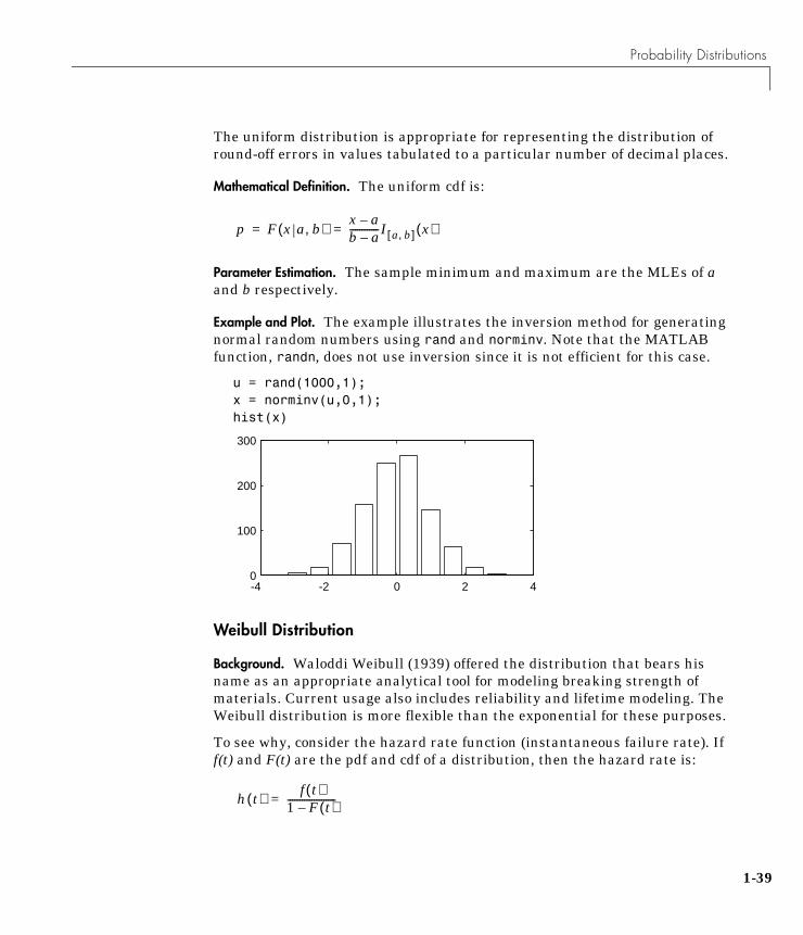
Example and Plot. The example illustrates the inversion method for generatingnormal random numbers using rand and norminv. Note that the MATLABfunction, randn, does not use inversion since it is not efficient for this case.
u = rand(1000,1);x = norminv(u,0,1);hist(x)
Weibull Distribution
Background. Waloddi Weibull (1939) offered the distribution that bears hisname as an appropriate analytical tool for modeling breaking strength ofmaterials. Current usage also includes reliability and lifetime modeling. TheWeibull distribution is more flexible than the exponential for these purposes.
To see why, consider the hazard rate function (instantaneous failure rate). Iff(t) and F(t) are the pdf and cdf of a distribution, then the hazard rate is:
p F x a b,( )x a–b a–------------I a b,[ ] x( )= =
-4 -2 0 2 40
100
200
300
h t( ) f t( )1 F t( )–--------------------=
1-39
1 Tutorial
1-4
Substituting the pdf and cdf of the exponential distribution for f(t) and F(t)above yields a constant. The example on the next page shows that the hazardrate for the Weibull distribution can vary.
Mathematical Definition. The Weibull pdf is:
Parameter Estimation. Suppose we want to model the tensile strength of a thinfilament using the Weibull distribution. The function weibfit give MLEs andconfidence intervals for the Weibull parameters.
strength = weibrnd(0.5,2,100,1); % Simulated strengths.[p, ci] = weibfit(strength)
p =
0.4746 1.9582
ci =
0.3851 1.6598 0.5641 2.2565
The default 95% confidence interval for each parameter contains the “true”value.
Example and Plot. The exponential distribution has a constant hazard function,which is not generally the case for the Weibull distribution.
y f x a b,( ) abxb 1– e axb– I 0 ∞,( ) x( )= =
0
Probability Distributions
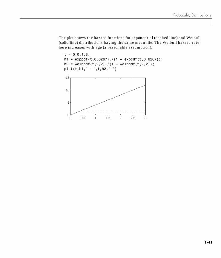
The plot shows the hazard functions for exponential (dashed line) and Weibull(solid line) distributions having the same mean life. The Weibull hazard ratehere increases with age (a reasonable assumption).
t = 0:0.1:3;h1 = exppdf(t,0.6267)./(1 – expcdf(t,0.6267));h2 = weibpdf(t,2,2)./(1 – weibcdf(t,2,2));plot(t,h1,'– –',t,h2,'–')
0 0.5 1 1.5 2 2.5 30
5
10
15
1-41

1 Tutorial
1-4
Descriptive StatisticsData samples can have thousands (even millions) of values. Descriptivestatistics are a way to summarize this data into a few numbers that containmost of the relevant information.
Measures of Central Tendency (Location)The purpose of measures of central tendency is to locate the data values on thenumber line. In fact, another term for these statistics is measures of location.
The table gives the function names and descriptions.
The average is a simple and popular estimate of location. If the data samplecomes from a normal distribution, then the sample average is also optimal(MVUE of µ).
Unfortunately, outliers, data entry errors, or glitches exist in almost all realdata. The sample average is sensitive to these problems. One bad data valuecan move the average away from the center of the rest of the data by anarbitrarily large distance.
The median and trimmed mean are two measures that are resistant (robust) tooutliers. The median is the 50th percentile of the sample, which will onlychange slightly if you add a large perturbation to any value. The idea behindthe trimmed mean is to ignore a small percentage of the highest and lowestvalues of a sample for determining the center of the sample.
Measures of Location
geomean Geometric Mean.
harmmean Harmonic Mean.
mean Arithmetic average (in MATLAB).
median 50th percentile (in MATLAB).
trimmean Trimmed Mean.
2
Descriptive Statistics
The geometric mean and harmonic mean, like the average, are not robust tooutliers. They are useful when the sample is distributed lognormal or heavilyskewed.
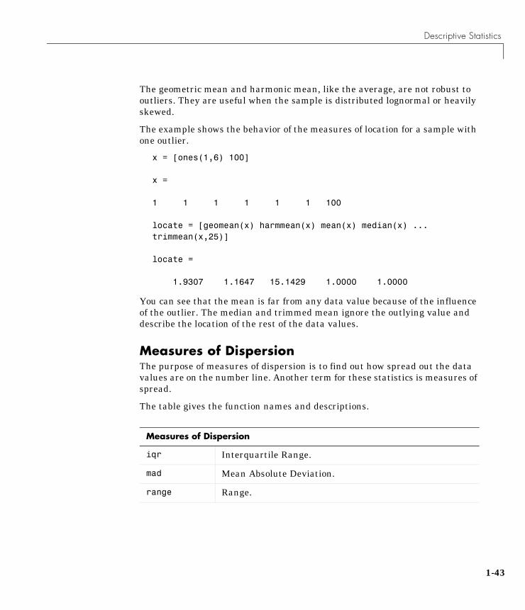
The example shows the behavior of the measures of location for a sample withone outlier.
x = [ones(1,6) 100]
x =
1 1 1 1 1 1 100
locate = [geomean(x) harmmean(x) mean(x) median(x) ...trimmean(x,25)]
locate =
1.9307 1.1647 15.1429 1.0000 1.0000
You can see that the mean is far from any data value because of the influenceof the outlier. The median and trimmed mean ignore the outlying value anddescribe the location of the rest of the data values.
Measures of DispersionThe purpose of measures of dispersion is to find out how spread out the datavalues are on the number line. Another term for these statistics is measures ofspread.
The table gives the function names and descriptions.
Measures of Dispersion
iqr Interquartile Range.
mad Mean Absolute Deviation.
range Range.
1-43
1 Tutorial
1-4
The range (the difference between the maximum and minimum values) is thesimplest measure of spread. But if there is an outlier in the data, it will be theminimum or maximum value. Thus, the range is not robust to outliers.
The standard deviation and the variance are popular measures of spread thatare optimal for normally distributed samples. The sample variance is theMVUE of the normal parameter σ2. The standard deviation is the square rootof the variance and has the desirable property of being in the same units as thedata. That is, if the data is in meters the standard deviation is in meters aswell. The variance is in meters2, which is more difficult to interpret.
Neither the standard deviation nor the variance is robust to outliers. A datavalue that is separate from the body of the data can increase the value of thestatistics by an arbitrarily large amount.
The Mean Absolute Deviation (MAD) is also sensitive to outliers. But the MADdoes not move quite as much as the standard deviation or variance in responseto bad data.
The Interquartile Range (IQR) is the difference between the 75th and 25thpercentile of the data. Since only the middle 50% of the data affects thismeasure, it is robust to outliers.
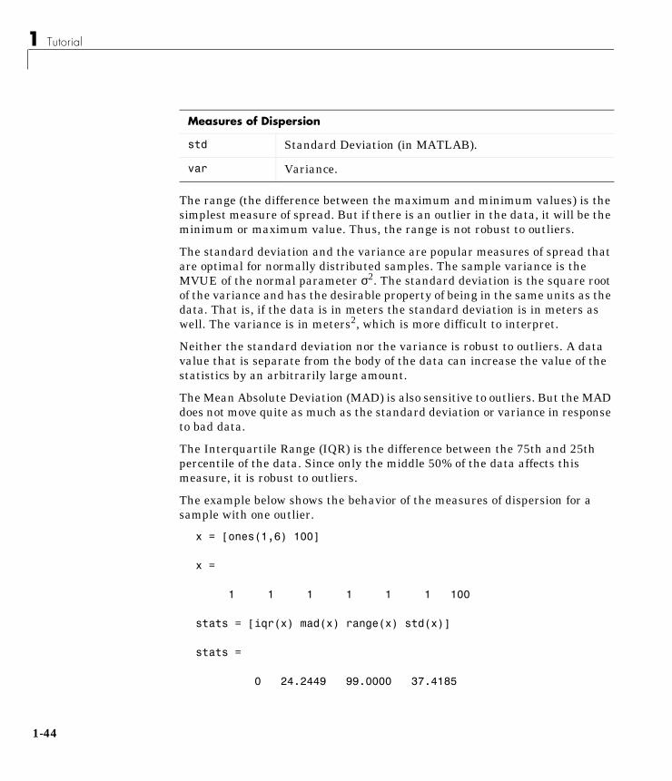
The example below shows the behavior of the measures of dispersion for asample with one outlier.
x = [ones(1,6) 100]
x =
1 1 1 1 1 1 100
stats = [iqr(x) mad(x) range(x) std(x)]
stats =
0 24.2449 99.0000 37.4185
std Standard Deviation (in MATLAB).
var Variance.
Measures of Dispersion
4
Descriptive Statistics
Functions for Data with Missing Values (NaNs)Most real-world datasets have one or more missing elements. It is convenientto code missing entries in a matrix as NaN (Not a Number.)
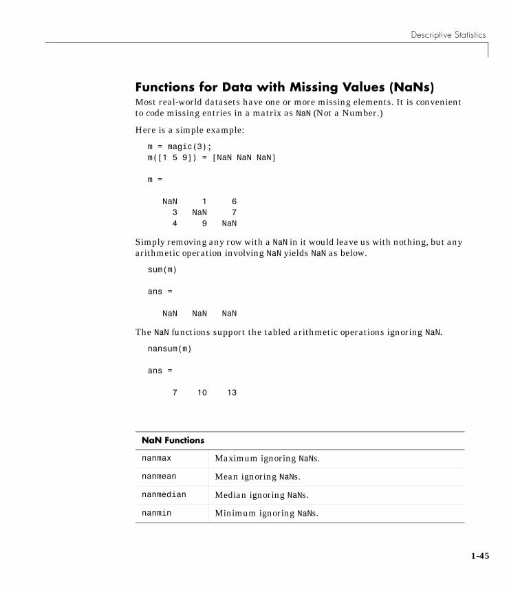
Here is a simple example:
m = magic(3);m([1 5 9]) = [NaN NaN NaN]
m =
NaN 1 6 3 NaN 7 4 9 NaN
Simply removing any row with a NaN in it would leave us with nothing, but anyarithmetic operation involving NaN yields NaN as below.
sum(m)
ans =
NaN NaN NaN
The NaN functions support the tabled arithmetic operations ignoring NaN.
nansum(m)
ans =
7 10 13
NaN Functions
nanmax Maximum ignoring NaNs.
nanmean Mean ignoring NaNs.
nanmedian Median ignoring NaNs.
nanmin Minimum ignoring NaNs.
1-45
1 Tutorial
1-4
Percentiles and Graphical DescriptionsTrying to describe a data sample with two numbers, a measure of location anda measure of spread, is frugal but may be misleading.
Another option is to compute a reasonable number of the sample percentiles.This provides information about the shape of the data as well as its locationand spread.
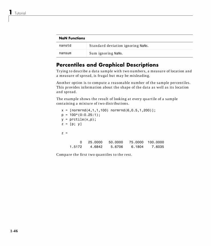
The example shows the result of looking at every quartile of a samplecontaining a mixture of two distributions.
x = [normrnd(4,1,1,100) normrnd(6,0.5,1,200)];p = 100*(0:0.25:1);y = prctile(x,p);z = [p; y]
z =
0 25.0000 50.0000 75.0000 100.0000 1.5172 4.6842 5.6706 6.1804 7.6035
Compare the first two quantiles to the rest.
nanstd Standard deviation ignoring NaNs.
nansum Sum ignoring NaNs.
NaN Functions
6

Descriptive Statistics
The box plot is a graph for descriptive statistics. The graph below is a box plotof the data above.
boxplot(x)
The long lower tail and plus signs show the lack of symmetry in the samplevalues. For more information on box plots see page 1-103.
The histogram is a complementary graph.
hist(x)
The BootstrapIn the last decade the statistical literature has examined the properties ofresampling as a means to acquire information about the uncertainty ofstatistical estimators.
The bootstrap is a procedure that involves choosing random samples withreplacement from a data set and analyzing each sample the same way.Sampling with replacement means that every sample is returned to the data setafter sampling. So a particular data point from the original data set could
1
2
3
4
5
6
7
Val
ues
Column Number
1 2 3 4 5 6 7 80
20
40
60
80
100
1-47

1 Tutorial
1-4
appear multiple times in a given bootstrap sample. The number of elements ineach bootstrap sample equals the number of elements in the original data set.The range of sample estimates we obtain allows us to establish the uncertaintyof the quantity we are estimating.
Here is an example taken from Efron and Tibshirani (1993) comparing LSATscores and subsequent law school GPA for a sample of 15 law schools.
load lawdataplot(lsat,gpa,'+')lsline
The least squares fit line indicates that higher LSAT scores go with higher lawschool GPAs. But how sure are we of this conclusion? The plot gives us someintuition but nothing quantitative.
We can calculate the correlation coefficient of the variables using the corrcoeffunction.
rhohat = corrcoef(lsat,gpa)
rhohat =
1.0000 0.7764 0.7764 1.0000
Now we have a number, 0.7764, describing the positive connection betweenLSAT and GPA, but though 0.7764 may seem large, we still do not know if it isstatistically significant.
Using the bootstrp function we can resample the lsat and gpa vectors asmany times as we like and consider the variation in the resulting correlationcoefficients.
540 560 580 600 620 640 660 6802.6
2.8
3
3.2
3.4
3.6
8

Descriptive Statistics
Here is an example:
rhos1000 = bootstrp(1000,'corrcoef',lsat,gpa);
This command resamples the lsat and gpa vectors 1000 times and computesthe corrcoef function on each sample. Here is a histogram of the result.
hist(rhos1000(:,2),30)
Nearly all the estimates lie on the interval [0.4 1.0].
This is strong quantitative evidence that LSAT and subsequent GPA arepositively correlated. Moreover, it does not require us to make any strongassumptions about the probability distribution of the correlation coefficient.
0.2 0.4 0.6 0.8 10
20
40
60
80
100
1-49

1 Tutorial
1-5
Cluster AnalysisCluster analysis, also called segmentation analysis or taxonomy analysis, is away to partition a set of objects into groups, or clusters, in such a way that theprofiles of objects in the same cluster are very similar and the profiles of objectsin different clusters are quite distinct.
Cluster analysis can be performed on many different types of datasets. Forexample, a dataset might contain a number of observations of subjects in astudy where each observation contains a set of variables.
Many different fields of study, such as engineering, zoology, medicine,linguistics, anthropology, psychology, and marketing, have contributed to thedevelopment of clustering techniques and the application of such techniques.For example, cluster analysis can be used to find two similar groups for theexperiment and control groups in a study. In this way, if statistical differencesare found in the groups, they can be attributed to the experiment and not toany initial difference between the groups.
Terminology and Basic ProcedureTo perform cluster analysis on a dataset using the Statistics Toolbox functions,follow this procedure:
1 Find the similarity or dissimilarity between every pair of objects inthe dataset. In this step, you calculate the distance between objects usingthe pdist function. The pdist function supports many different ways tocompute this measurement. See the section “Finding the SimilaritiesBetween Objects” for more information.
2 Group the objects into a binary, hierarchical cluster tree. In this step,you link together pairs of objects that are in close proximity using thelinkage function. The linkage function uses the distance informationgenerated in step 1 to determine the proximity of objects to each other. Asobjects are paired into binary clusters, the newly formed clusters aregrouped into larger clusters until a hierarchical tree is formed. See thesection “Defining the Links Between Objects” for more information.
3 Determine where to divide the hierarchical tree into clusters. In thisstep, you divide the objects in the hierarchical tree into clusters using thecluster function. The cluster function can create clusters by detecting
0
Cluster Analysis
natural groupings in the hierarchical tree or by cutting off the hierarchicaltree at an arbitrary point. See the section “Creating Clusters” for moreinformation.
The following sections provide more information about each of these steps.
Note The Statistics Toolbox includes a convenience function, clusterdata,which performs all these steps for you. You do not need to execute the pdist,linkage, or cluster functions separately. However, the clusterdata functiondoes not give you access to the options each of the individual routines offers.For example, if you use the pdist function, you can choose the distancecalculation method.
Finding the Similarities Between ObjectsYou use the pdist function to calculate the distance between every pair ofobjects in a dataset. For a dataset made up of m objects, there are
pairs in the dataset. The result of this computation is commonlyknown as a similarity matrix (or dissimilarity matrix).
There are many ways to calculate this distance information. By default, thepdist function calculates the Euclidean distance between objects; however,you can specify one of several other options. See pdist for more information.
Note You can optionally normalize the values in the dataset beforecalculating the distance information. In a real world dataset, variables can bemeasured against different scales. For example, one variable can measure IQtest scores and another variable measure head circumference. Thesediscrepancies can distort the proximity calculations. Using the zscorefunction, you can convert all the values in the dataset to use the sameproportional scale. See the zscore function for more information.
m m 1–( )⋅ 2⁄
1-51

1 Tutorial
1-5
For example, consider a data set, X, made up of five objects where each objectis a set of x,y coordinates.
You can define this dataset as a matrix, X = [1 2;2.5 4.5;2 2;4 1.5;4 2.5],and pass it to pdist. The pdist function calculates the distance between object1 and object 2, object 1 and object 3, and so on until the distances between allthe pairs have been calculated. The following figure plots these objects in agraph. The distance between object 2 and object 3 is shown to illustrate oneinterpretation of distance.
Object Value
1 1 2
2 2.5 4.5
3 2 2
4 4 1.5
5 4 2.5
1
1
5
2 43
4
3
2
5
distance
1 3 4
5
2
2

Cluster Analysis
Returning Distance Information The pdist function returns this distance information in a vector, Y,where eachelement contains the distance between a pair of objects.
Y = pdist(X)Y = Columns 1 through 7 2.9155 1.0000 3.0414 3.0414 2.5495 3.3541 2.5000 Columns 8 through 10 2.0616 2.0616 1.0000
To make it easier to see the relationship between the distance informationgenerated by pdist and the objects in the original dataset, you can reformatthe distance vector into a matrix using the squareform function. In this matrix,element i,j corresponds to the distance between object i and object j in theoriginal dataset. In the following example, element 1,1 represents the distancebetween object 1 and itself (which is zero). Element 1,2 represents the distancebetween object 1 and object 2, and so on.
squareform(Y)ans = 0 2.9155 1.0000 3.0414 3.0414 2.9155 0 2.5495 3.3541 2.5000 1.0000 2.5495 0 2.0616 2.0616 3.0414 3.3541 2.0616 0 1.0000 3.0414 2.5000 2.0616 1.0000 0
Defining the Links Between ObjectsOnce the proximity between objects in the dataset has been computed, you candetermine which objects in the data set should be grouped together intoclusters, using the linkage function. The linkage function takes the distanceinformation generated by pdist and links pairs of objects that are closetogether into binary clusters (clusters made up of two objects). The linkagefunction then links these newly formed clusters to other objects to create biggerclusters until all the objects in the original data set are linked together in ahierarchical tree.
1-53
1 Tutorial
1-5
For example, given the distance vector, Y, generated by pdist from the sampledataset of x and y coordinates, the linkage function generates a hierarchicalcluster tree, returning the linkage information in a matrix, Z.
Z = linkage(Y)Z = 1.0000 3.0000 1.0000 4.0000 5.0000 1.0000 6.0000 7.0000 2.0616 8.0000 2.0000 2.5000
In this output, each row identifies a link. The first two columns identify theobjects that have been linked, that is, object 1, object 2, and so on. The thirdcolumn contains the distance between these objects. For the sample dataset ofx and y coordinates, the linkage function begins by grouping together objects1 and 3, which have the closest proximity (distance value = 1.0000). Thelinkage function continues by grouping objects 4 and 5, which also have adistance value of 1.0000.
The third row indicates that the linkage function grouped together objects 6and 7. If our original sample dataset contained only 5 objects, what are objects6 and 7? Object 6 is the newly formed binary cluster created by the grouping ofobjects 1 and 3. When the linkage function groups two objects together into anew cluster, it must assign the cluster a unique index value, starting with thevalue m+1, where m is the number of objects in the original dataset. (Values 1through m are already used by the original dataset.) Object 7 is the index forthe cluster formed by objects 4 and 5.
As the final cluster, the linkage function grouped object 8, the newly formedcluster made up of objects 6 and 7, with object 2 from the original dataset. The
4
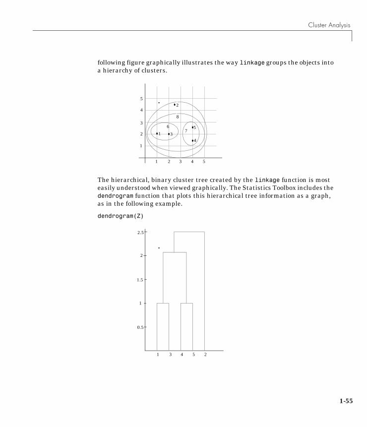
Cluster Analysis
following figure graphically illustrates the way linkage groups the objects intoa hierarchy of clusters.
The hierarchical, binary cluster tree created by the linkage function is mosteasily understood when viewed graphically. The Statistics Toolbox includes thedendrogram function that plots this hierarchical tree information as a graph,as in the following example.
dendrogram(Z)
1
1
5
2 43
4
3
2
5
67
8
1
2
34
5
0.5
1
2.5
3 54
2
1.5
1
2
1-55
1 Tutorial
1-5
In the figure, the numbers along the horizontal axis represent the indices of theobjects in the original dataset. The links between objects are represented asupside down U-shaped lines. The height of the U indicates the distancebetween the objects. For example, the link representing the cluster containingobjects 1 and 3 has a height of 1. For more information about creating adendrogram diagram, see the dendrogram function reference page.
Evaluating Cluster FormationAfter linking the objects in a dataset into a hierarchical cluster tree, you maywant to verify that the tree represents significant similarity groupings. Inaddition, you may want more information about the links between the objects.The Statistics Toolbox provides functions to perform both these tasks.
Verifying the Cluster TreeOne way to measure the validity of the cluster information generated by thelinkage function is to compare it with the original proximity data generated bythe pdist function. If the clustering is valid, the linking of objects in the clustertree should have a strong correlation with the distances between objects in thedistance vector. The cophenet function compares these two sets of values andcomputes their correlation, returning a value called the cophenetic correlationcoefficient. The closer the value of the cophenetic correlation coefficient is to 1,the better the clustering solution.
You can use the cophenetic correlation coefficient to compare the results ofclustering the same dataset using different distance calculation methods orclustering algorithms.
For example, you can use the cophenet function to evaluate the clusterscreated for the sample dataset
c = cophenet(Z,Y)c = 0.8573
where Z is the matrix output by the linkage function and Y is the distancevector output by the pdist function.
6
Cluster Analysis
Execute pdist again on the same dataset, this time specifying the City Blockmetric. After running the linkage function on this new pdist output, use thecophenet function to evaluate the clustering using a different distance metric.
c = cophenet(Z,Y)
c =0.9289
The cophenetic correlation coefficient shows a stronger correlation when theCity Block metric is used.
Getting More Information about Cluster LinksOne way to determine the natural cluster divisions in a dataset is to comparethe length of each link in a cluster tree with the lengths of neighboring linksbelow it in the tree.
If a link is approximately the same length as neighboring links, it indicatesthat there are similarities between the objects joined at this level of thehierarchy. These links are said to exhibit a high level of consistency.
If the length of a link differs from neighboring links, it indicates that there aredissimilarities between the objects at this level in the cluster tree. This link issaid to be inconsistent with the links around it. In cluster analysis,inconsistent links can indicate the border of a natural division in a dataset. Thecluster function uses a measure of inconsistency to determine where to dividea dataset into clusters. (See “Creating Clusters” for more information.)
To illustrate, the following example creates a dataset of random numbers withthree deliberate natural groupings. In the dendrogram, note how the objectstend to collect into three groups. These three groups are then connected bythree longer links. These longer links are inconsistent when compared with thelinks below them in the hierarchy.
1-57

1 Tutorial
1-5
rand('seed',3)X = [rand(10,2)+1;rand(10,2)+2;rand(10,2)+3];Y = pdist(X);Z = linkage(Y);dendrogram(Z);
The relative consistency of each link in a hierarchical cluster tree can bequantified and expressed as the inconsistency coefficient. This value comparesthe length of a link in a cluster hierarchy with the average length ofneighboring links. If the object is consistent with those around it, it will have alow inconsistency coefficient. If the object is inconsistent with those around it,it will have a higher inconsistency coefficient.
To generate a listing of the inconsistency coefficient for each link the clustertree, use the inconsistent function. The inconsistent function compares
0
0.1
0.2
0.3
0.4
0.5
0.6
0.7
23 25 29 30 27 28 26 24 21 22 11 12 15 13 16 18 20 14 17 19 1 2 7 3 6 8 9 10 4 5
These links show consistency
These links show inconsistency, when compared to links below them.
8
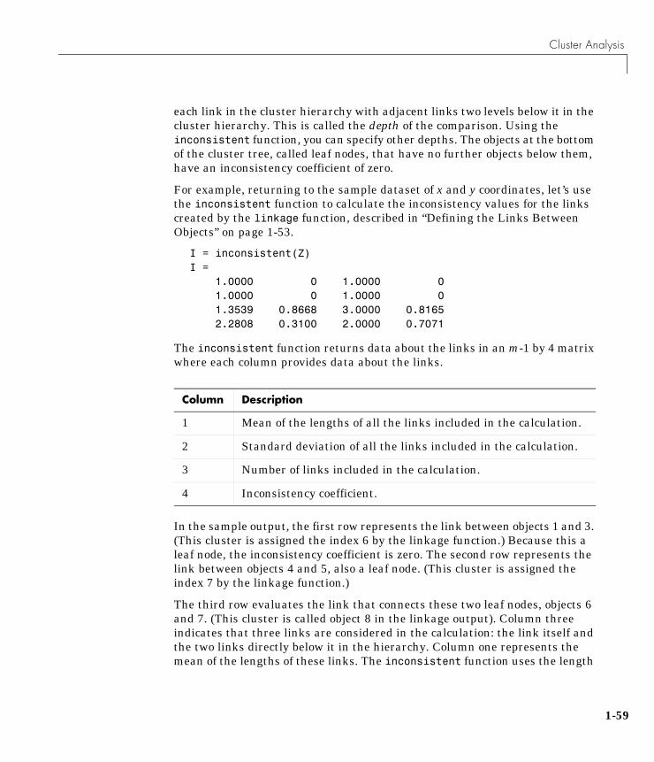
Cluster Analysis
each link in the cluster hierarchy with adjacent links two levels below it in thecluster hierarchy. This is called the depth of the comparison. Using theinconsistent function, you can specify other depths. The objects at the bottomof the cluster tree, called leaf nodes, that have no further objects below them,have an inconsistency coefficient of zero.
For example, returning to the sample dataset of x and y coordinates, let’s usethe inconsistent function to calculate the inconsistency values for the linkscreated by the linkage function, described in “Defining the Links BetweenObjects” on page 1-53.
I = inconsistent(Z)I = 1.0000 0 1.0000 0 1.0000 0 1.0000 0 1.3539 0.8668 3.0000 0.8165 2.2808 0.3100 2.0000 0.7071
The inconsistent function returns data about the links in an m-1 by 4 matrixwhere each column provides data about the links.
In the sample output, the first row represents the link between objects 1 and 3.(This cluster is assigned the index 6 by the linkage function.) Because this aleaf node, the inconsistency coefficient is zero. The second row represents thelink between objects 4 and 5, also a leaf node. (This cluster is assigned theindex 7 by the linkage function.)
The third row evaluates the link that connects these two leaf nodes, objects 6and 7. (This cluster is called object 8 in the linkage output). Column threeindicates that three links are considered in the calculation: the link itself andthe two links directly below it in the hierarchy. Column one represents themean of the lengths of these links. The inconsistent function uses the length
Column Description
1 Mean of the lengths of all the links included in the calculation.
2 Standard deviation of all the links included in the calculation.
3 Number of links included in the calculation.
4 Inconsistency coefficient.
1-59
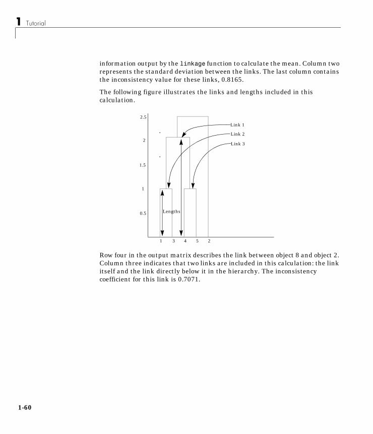
1 Tutorial
1-6
information output by the linkage function to calculate the mean. Column tworepresents the standard deviation between the links. The last column containsthe inconsistency value for these links, 0.8165.
The following figure illustrates the links and lengths included in thiscalculation.
Row four in the output matrix describes the link between object 8 and object 2.Column three indicates that two links are included in this calculation: the linkitself and the link directly below it in the hierarchy. The inconsistencycoefficient for this link is 0.7071.
0.5
1
2.5
3 54
2
1.5
1
2
Link 1
Lengths
Link 2
Link 3
0
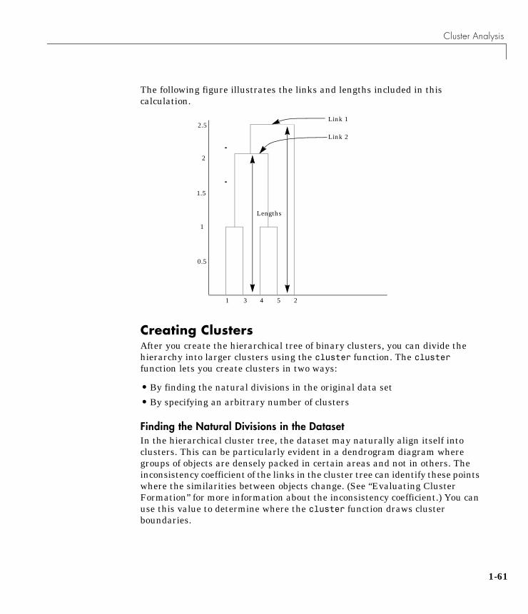
Cluster Analysis
The following figure illustrates the links and lengths included in thiscalculation.
Creating Clusters After you create the hierarchical tree of binary clusters, you can divide thehierarchy into larger clusters using the cluster function. The clusterfunction lets you create clusters in two ways:
• By finding the natural divisions in the original data set
• By specifying an arbitrary number of clusters
Finding the Natural Divisions in the DatasetIn the hierarchical cluster tree, the dataset may naturally align itself intoclusters. This can be particularly evident in a dendrogram diagram wheregroups of objects are densely packed in certain areas and not in others. Theinconsistency coefficient of the links in the cluster tree can identify these pointswhere the similarities between objects change. (See “Evaluating ClusterFormation” for more information about the inconsistency coefficient.) You canuse this value to determine where the cluster function draws clusterboundaries.
0.5
1
2.5
3 54
2
1.5
1
2
Link 1
Lengths
Link 2
1-61

1 Tutorial
1-6
For example, if you use the cluster function to group the sample dataset intoclusters, specifying an inconsistency coefficient threshold of 0.9 as the value ofthe cutoff argument, the cluster function groups all the objects in the sampledataset into one cluster. In this case, none of the links in the cluster hierarchyhad an inconsistency coefficient greater than 0.9.
T = cluster(Z,0.9)T = 1 1 1 1 1
The cluster function outputs a vector, T, that is the same size as the originaldataset. Each element in this vector contains the number of the cluster intowhich the corresponding object from the original data set was placed.
If you lower the inconsistency coefficient threshold to 0.8, the cluster functiondivides the sample dataset into three separate clusters.
T = cluster(Z,0.8)T =
13122
This output indicates that objects 1 and 3 were placed in cluster 1, objects 4 and5 were placed in cluster 2, and object 2 was placed in cluster 3.
Specifying Arbitrary ClustersInstead of letting the cluster function create clusters determined by thenatural divisions in the data set, you can specify the number of clusters youwant created. In this case, the value of the cutoff argument specifies the pointin the cluster hierarchy at which to create the clusters.
2

Cluster Analysis
For example, you can specify that you want the cluster function to divide thesample dataset into two clusters. In this case, the cluster function creates onecluster containing objects 1, 3, 4, and 5 and another cluster containing object 2.
T = cluster(Z,2)T =
12111
To help you visualize how the cluster function determines how to create theseclusters, the following figure shows the dendrogram of the hierarchical clustertree. When you specify a value of 2, the cluster function draws an imaginaryhorizontal line across the dendrogram that bisects two vertical lines. All theobjects below the line belong to one of these two clusters.
0.5
1
2.5
3 54
2
1.5
1
2
cutoff = 2
1-63
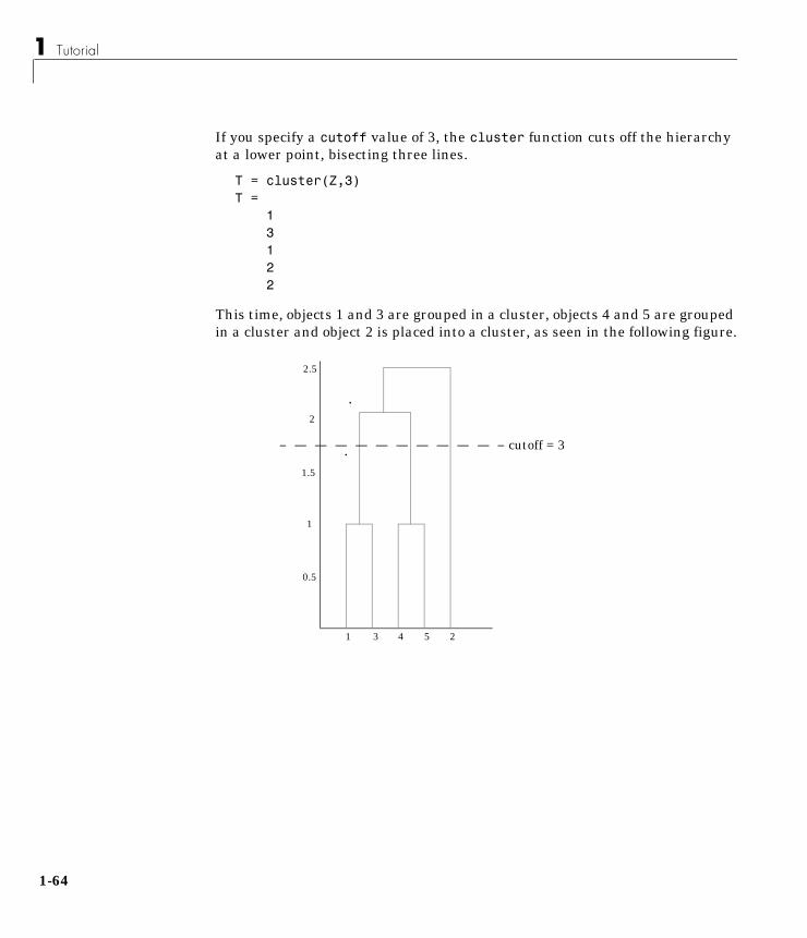
1 Tutorial
1-6
If you specify a cutoff value of 3, the cluster function cuts off the hierarchyat a lower point, bisecting three lines.
T = cluster(Z,3)T =
13122
This time, objects 1 and 3 are grouped in a cluster, objects 4 and 5 are groupedin a cluster and object 2 is placed into a cluster, as seen in the following figure.
0.5
1
2.5
3 54
2
1.5
1
2
cutoff = 3
4
Linear Models
Linear ModelsLinear models are problems that take the form
where:
• y is an n by 1 vector of observations.
• X is the n by p design matrix for the model.
• β is a p by 1 vector of parameters.
• ε is an n by 1 vector of random disturbances.
One-way analysis of variance (ANOVA), two-way ANOVA, polynomialregression, and multiple linear regression are specific cases of the linear model.
One-Way Analysis of Variance (ANOVA)The purpose of a one-way ANOVA is to find out whether data from severalgroups have a common mean. That is, to determine whether the groups areactually different in the measured characteristic.
One-way ANOVA is a simple special case of the linear model. The one-wayANOVA form of the model is
where:
• yij is a matrix of observations.
• α.j is a matrix whose columns are the group means. (The “dot j” notationmeans that α applies to all rows of the jth column.)
• εij is a matrix of random disturbances.
The model posits that the columns of y are a constant plus a randomdisturbance. You want to know if the constants are all the same.
The data below comes from a study by Hogg and Ledolter (1987) of bacteriacounts in shipments of milk. The columns of the matrix hogg representdifferent shipments. The rows are bacteria counts from cartons of milk chosen
y Xβ ε+=
yij α.j εij+=
1-65
1 Tutorial
1-6
randomly from each shipment. Do some shipments have higher counts thanothers?
load hoggp = anova1(hogg)
p =
1.1971e–04
hogg
hogg =
24 14 11 7 19 15 7 9 7 24 21 12 7 4 19 27 17 13 7 15 33 14 12 12 10 23 16 18 18 20
The standard ANOVA table has columns for the sums of squares, degrees offreedom, mean squares (SS/df), and F statistic.
You can use the F statistic to do a hypothesis test to find out if the bacteriacounts are the same. anova1 returns the p-value from this hypothesis test.
In this case the p-value is about 0.0001, a very small value. This is a strongindication that the bacteria counts from the different tankers are not the same.An F statistic as extreme as the observed F would occur by chance only once in10,000 times if the counts were truly equal.
The p-value returned by anova1 depends on assumptions about the randomdisturbances in the model equation. For the p-value to be correct, these
ANOVA Table
Source SS df MS F Columns 803 4 200.7 9.008Error 557.2 25 22.29Total 1360 29
6

Linear Models
disturbances need to be independent, normally distributed and have constantvariance.
You can get some graphic assurance that the means are different by looking atthe box plots in the second figure window displayed by anova1.
Since the notches in the box plots do not all overlap, this is strong confirmingevidence that the column means are not equal.
Two-Way Analysis of Variance (ANOVA)The purpose of two-way ANOVA is to find out whether data from severalgroups have a common mean. One-way ANOVA and two-way ANOVA differ inthat the groups in two-way ANOVA have two categories of definingcharacteristics instead of one.
Suppose an automobile company has two factories that both make three modelsof car. It is reasonable to ask if the gas mileage in the cars varies from factoryto factory as well as model to model.
There could be an overall difference in mileage due to a difference in theproduction methods between factories. There is probably a difference in themileage of the different models (irrespective of the factory) due to differencesin design specifications. These effects are called additive.
Finally, a factory might make high mileage cars in one model (perhaps becauseof a superior production line), but not be different from the other factory forother models. This effect is called an interaction. It is impossible to detect aninteraction unless there are duplicate observations for some combination offactory and car model.
1 2 3 4 5
5
10
15
20
25
30
Val
ues
Column Number
1-67
1 Tutorial
1-6
Two-way ANOVA is a special case of the linear model. The two-way ANOVAform of the model is
where:
• yijk is a matrix of observations.
• µ is a constant matrix of the overall mean.
• α.j is a matrix whose columns are the group means (the rows of α sum to 0).
• βi. is a matrix whose rows are the group means (the columns of β sum to 0).
• γij is a matrix of interactions (the rows and columns of γ sum to zero).
• εijk is a matrix of random disturbances.
The purpose of the example is to determine the effect of car model and factoryon the mileage rating of cars.
load mileagemileage
mileage =
33.3000 34.5000 37.4000 33.4000 34.8000 36.8000 32.9000 33.8000 37.6000 32.6000 33.4000 36.6000 32.5000 33.7000 37.0000 33.0000 33.9000 36.7000
cars = 3;p = anova2(mileage,cars)
p =
0.0000 0.0039 0.8411
There are three models of cars (columns) and two factories (rows). The reasonthere are six rows instead of two is that each factory provides three cars of eachmodel for the study. The data from the first factory is in the first three rows,and the data from the second factory is in the last three rows.
yijk µ α.j βi . γij εijk+ + + +=
8
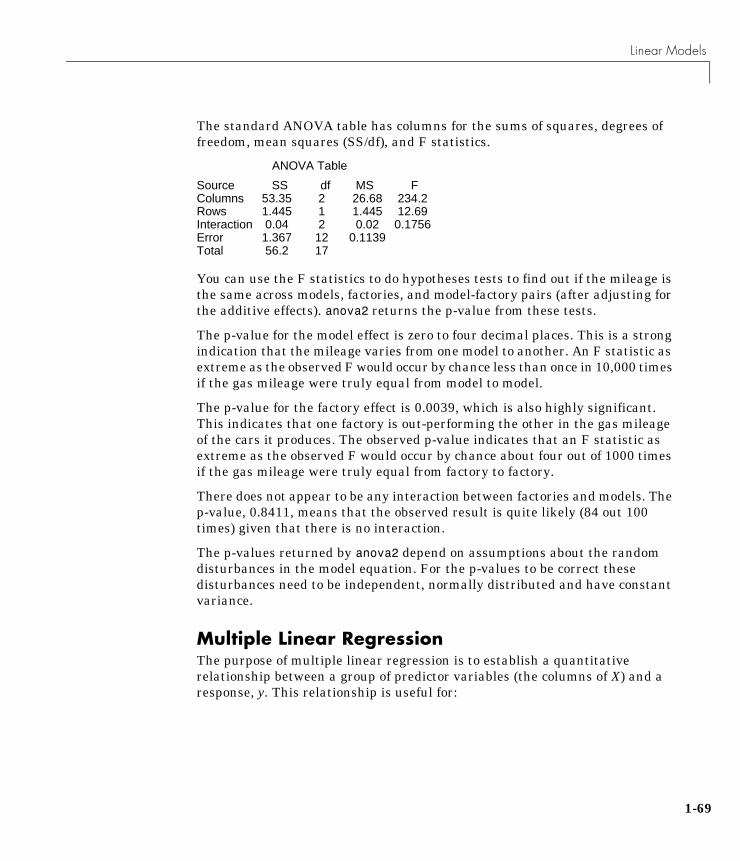
Linear Models
The standard ANOVA table has columns for the sums of squares, degrees offreedom, mean squares (SS/df), and F statistics.
You can use the F statistics to do hypotheses tests to find out if the mileage isthe same across models, factories, and model-factory pairs (after adjusting forthe additive effects). anova2 returns the p-value from these tests.
The p-value for the model effect is zero to four decimal places. This is a strongindication that the mileage varies from one model to another. An F statistic asextreme as the observed F would occur by chance less than once in 10,000 timesif the gas mileage were truly equal from model to model.
The p-value for the factory effect is 0.0039, which is also highly significant.This indicates that one factory is out-performing the other in the gas mileageof the cars it produces. The observed p-value indicates that an F statistic asextreme as the observed F would occur by chance about four out of 1000 timesif the gas mileage were truly equal from factory to factory.
There does not appear to be any interaction between factories and models. Thep-value, 0.8411, means that the observed result is quite likely (84 out 100times) given that there is no interaction.
The p-values returned by anova2 depend on assumptions about the randomdisturbances in the model equation. For the p-values to be correct thesedisturbances need to be independent, normally distributed and have constantvariance.
Multiple Linear RegressionThe purpose of multiple linear regression is to establish a quantitativerelationship between a group of predictor variables (the columns of X) and aresponse, y. This relationship is useful for:
ANOVA Table
Source SS df MS F Columns 53.35 2 26.68 234.2Rows 1.445 1 1.445 12.69Interaction 0.04 2 0.02 0.1756Error 1.367 12 0.1139Total 56.2 17
1-69
1 Tutorial
1-7
• Understanding which predictors have the most effect.
• Knowing the direction of the effect (i.e., increasing x increases/decreases y).
• Using the model to predict future values of the response when only thepredictors are currently known.
The linear model takes its common form
where:
• y is an n by 1 vector of observations.
• X is an n by p matrix of regressors.
• β is a p by 1 vector of parameters.
• ε is an n by 1 vector of random disturbances.
The solution to the problem is a vector, b, which estimates the unknown vectorof parameters, β. The least-squares solution is:
This equation is useful for developing later statistical formulas, but has poornumeric properties. regress uses QR decomposition of X followed by thebackslash operator to compute b. The QR decomposition is not necessary forcomputing b, but the matrix, R, is useful for computing confidence intervals.
You can plug b back into the model formula to get the predicted y values at thedata points.
Statisticians use a hat (circumflex) over a letter to denote an estimate of aparameter or a prediction from a model. The projection matrix H, is called thehat matrix, because it puts the “hat” on y.
The residuals are the difference between the observed and predicted y values.
y Xβ ε+=
b β X'X( )1–
X'y= =
y Xb Hy= =
H X X'X( )1–
X'=
r y y–= I H–( )= y
0
Linear Models
The residuals are useful for detecting failures in the model assumptions, sincethey correspond to the errors, ε, in the model equation. By assumption, theseerrors each have independent normal distributions with mean zero and aconstant variance.
The residuals, however, are correlated and have variances that depend on thelocations of the data points. It is a common practice to scale (“Studentize”) theresiduals so they all have the same variance.
In the equation below, the scaled residual, ti, has a Student’s t distribution with(n–p) degrees of freedom.
where:
• ti is the scaled residual for the ith data point.
• ri is the raw residual for the ith data point.
• n is the sample size.
• p is the number of parameters in the model.
• hi is the ith diagonal element of H.
The left-hand side of the second equation is the estimate of the variance of theerrors excluding the ith data point from the calculation.
A hypothesis test for outliers involves comparing ti with the critical values ofthe t distribution. If ti is large, this casts doubt on the assumption that thisresidual has the same variance as the others.
A confidence interval for the mean of each error is:
ti
ri
σ i( ) 1 hi–----------------------------=
σ2
i( )r 2
n p– 1–----------------------
ri2
n p– 1–( ) 1 hi–( )-----------------------------------------------–=
ci ri t1
α2--- ν,–
± σ i( ) 1 hi–=
1-71
1 Tutorial
1-7
Confidence intervals that do not include zero are equivalent to rejecting thehypothesis (at a significance probability of α) that the residual mean is zero.Such confidence intervals are good evidence that the observation is an outlierfor the given model.
ExampleThe example comes from Chatterjee and Hadi (1986) in a paper on regressiondiagnostics. The dataset (originally from Moore (1975)) has five predictorvariables and one response.
load mooreX = [ones(size(moore,1),1) moore(:,1:5)];
The matrix, X, has a column of ones, then one column of values for each of thefive predictor variables. The column of ones is necessary for estimating they-intercept of the linear model.
y = moore(:,6);[b,bint,r,rint,stats] = regress(y,X);
The y-intercept is b(1), which corresponds to the column index of the columnof ones.
stats
stats =
0.8107 11.9886 0.0001
The elements of the vector stats are the regression R2 statistic, the F statistic(for the hypothesis test that all the regression coefficients are zero), and thep-value associated with this F statistic.
2

Linear Models
R2 is 0.8107 indicating the model accounts for over 80% of the variability in theobservations. The F statistic of about 12 and its p-value of 0.0001 indicate thatit is highly unlikely that all of the regression coefficients are zero.
rcoplot(r,rint)
The plot shows the residuals plotted in case order (by row). The 95% confidenceintervals about these residuals are plotted as error bars. The first observationis an outlier since its error bar does not cross the zero reference line.
Quadratic Response Surface ModelsResponse Surface Methodology (RSM) is a tool for understanding thequantitative relationship between multiple input variables and one outputvariable.
Consider one output, z, as a polynomial function of two inputs, x and y..z = f(x,y)describes a two dimensional surface in the space (x,y,z). Of course, you can haveas many input variables as you want and the resulting surface becomes ahyper-surface.
For three inputs (x1, x2, x3) the equation of a quadratic response surface is:
y = b0 + b1x1 + b2x2 + b3x3 + ... (linear terms)
b12x1x2 + b13x1x3 + b23x2x3 + ... (interaction terms)
b11x12 + b22x2
2 + b33x32 (quadratic terms)
It is difficult to visualize a k-dimensional surface in k+1 dimensional spacewhen k>2. The function rstool is a GUI designed to make this visualizationmore intuitive.
0 5 10 15 20
-0.5
0
0.5R
esid
uals
Case Number
1-73
1 Tutorial
1-7
Exploring Graphs of Multidimensional PolynomialsThe function rstool is useful for fitting response surface models. The purposeof rstool is larger than just fitting and prediction for polynomial models. ThisGUI provides an environment for exploration of the graph of amultidimensional polynomial.
You can learn about rstool by trying the commands below. The chemistrybehind the data in reaction.mat deals with reaction kinetics as a function ofthe partial pressure of three chemical reactants: hydrogen, n-pentane, andisopentane.
load reactionrstool(reactants,rate,'quadratic',0.01,xn,yn)
You will see a “vector” of three plots. The dependent variable of all three plotsis the reaction rate. The first plot has hydrogen as the independent variable.The second and third plots have n-pentane and isopentane respectively.
Each plot shows the fitted relationship of the reaction rate to the independentvariable at a fixed value of the other two independent variables. The fixedvalue of each independent variable is in an editable text box below each axis.You can change the fixed value of any independent variable by either typing anew value in the box or by dragging any of the 3 vertical lines to a new position.
When you change the value of an independent variable, all the plots update toshow the current picture at the new point in the space of the independentvariables.
Note that while this example only uses three reactants, rstool canaccommodate an arbitrary number of independent variables. Interpretabilitymay be limited by the size of the monitor for large numbers of inputs.
The GUI also has two pop-up menus. The Export menu facilitates savingvarious important variables in the GUI to the base workspace. Below theExport menu there is another menu that allows you to change the order of thepolynomial model from within the GUI. If you used the commands above, thismenu will have the string Full Quadratic. Other choices are:
• Linear – has the constant and first order terms only.
• Pure Quadratic – includes constant, linear and squared terms.
• Interactions – includes constant, linear, and cross product terms.
4
Linear Models
Stepwise Regression Stepwise regression is a technique for choosing the variables to include in amultiple regression model. Forward stepwise regression starts with no modelterms. At each step it adds the most statistically significant term (the one withthe highest F statistic or lowest p-value) until there are none left. Backwardstepwise regression starts with all the terms in the model and removes theleast significant terms until all the remaining terms are statisticallysignificant. It is also possible to start with a subset of all the terms and thenadd significant terms or remove insignificant terms.
An important assumption behind the method is that some input variables in amultiple regression do not have an important explanatory effect on theresponse. If this assumption is true, then it is a convenient simplification tokeep only the statistically significant terms in the model.
One common problem in multiple regression analysis is multicollinearity of theinput variables. The input variables may be as correlated with each other asthey are with the response. If this is the case, the presence of one input variablein the model may mask the effect of another input. Stepwise regression used asa canned procedure is a dangerous tool because the resulting model mayinclude different variables depending on the choice of starting model andinclusion strategy.
The Statistics Toolbox uses an interactive graphical user interface (GUI) toprovide a more understandable comparison of competing models. You canexplore the GUI using the Hald (1960) data set. Here are the commands to getstarted.
load haldstepwise(ingredients,heat)
The Hald data come from a study of the heat of reaction of various cementmixtures. There are 4 components in each mixture, and the amount of heatproduced depends on the amount of each ingredient in the mixture.
Stepwise Regression Interactive GUI The interface consists of three interactively linked figure windows:
• The Stepwise Regression Plot
• The Stepwise Regression Diagnostics Table
• The Stepwise History Plot
1-75
1 Tutorial
1-7
All three windows have hot regions. When your mouse is above one of theseregions, the pointer changes from an arrow to a circle. Clicking on this pointinitiates some activity in the interface.
Stepwise Regression PlotThis plot shows the regression coefficient and confidence interval for everyterm (in or out of the model). The green lines represent terms in the modelwhile red lines indicate that the term is not currently in the model.
Statistically significant terms are solid lines. Dotted lines show that the fittedcoefficient is not significantly different from zero.
Clicking on a line in this plot toggles its state. That is, a term in the model(green line) gets removed (turns red), and terms out of the model (red line)enter the model (turn green).
The coefficient for a term out of the model is the coefficient resulting fromadding that term to the current model.
Scale Inputs. Pressing this button centers and normalizes the columns of theinput matrix to have a standard deviation of one.
Export. This pop-up menu allows you to export variables from the stepwisefunction to the base workspace.
Close. The Close button removes all the figure windows.
Stepwise Regression Diagnostics FigureThis table is a quantitative view of the information in the Stepwise RegressionPlot. The table shows the Hald model with the second and third terms removed.
6
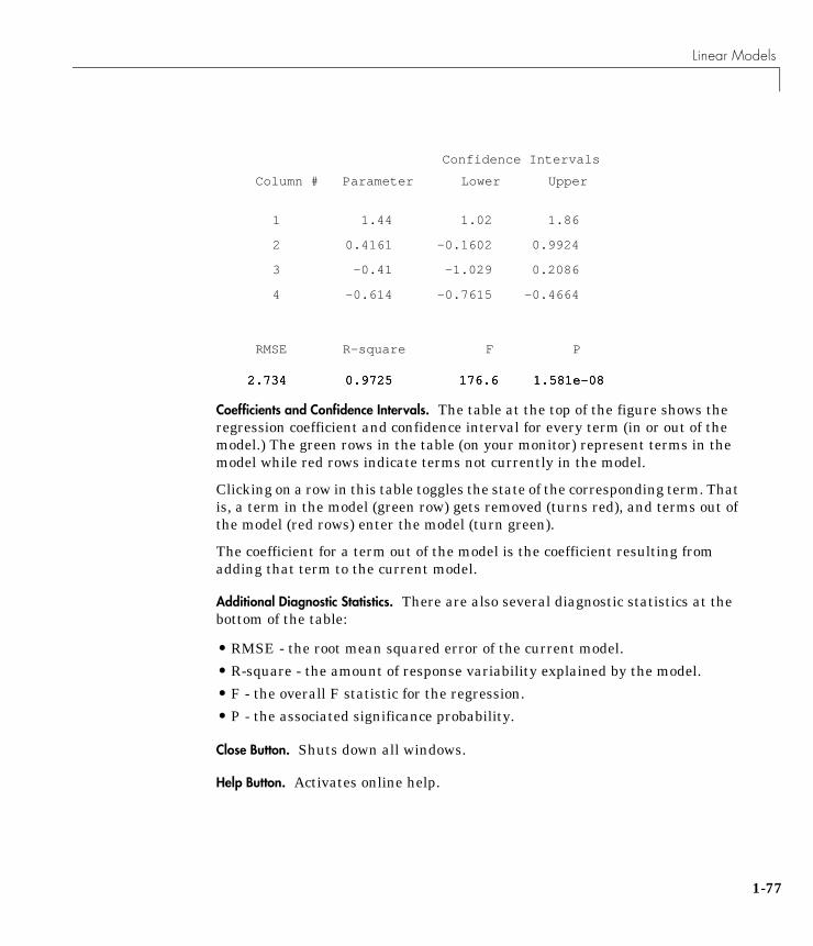
Linear Models
Coefficients and Confidence Intervals. The table at the top of the figure shows theregression coefficient and confidence interval for every term (in or out of themodel.) The green rows in the table (on your monitor) represent terms in themodel while red rows indicate terms not currently in the model.
Clicking on a row in this table toggles the state of the corresponding term. Thatis, a term in the model (green row) gets removed (turns red), and terms out ofthe model (red rows) enter the model (turn green).
The coefficient for a term out of the model is the coefficient resulting fromadding that term to the current model.
Additional Diagnostic Statistics. There are also several diagnostic statistics at thebottom of the table:
• RMSE - the root mean squared error of the current model.
• R-square - the amount of response variability explained by the model.
• F - the overall F statistic for the regression.
• P - the associated significance probability.
Close Button. Shuts down all windows.
Help Button. Activates online help.
Confidence Intervals
Column #
RMSE
Parameter
R-square
Lower
F
Upper
P
1 1.44 1.02 1.86
2.734 0.9725 176.6 1.581e-08
2 0.4161 -0.1602 0.9924
2.734 0.9725 176.6 1.581e-08
3 -0.41 -1.029 0.2086
2.734 0.9725 176.6 1.581e-08
4 -0.614 -0.7615 -0.4664
2.734 0.9725 176.6 1.581e-08
1-77

1 Tutorial
1-7
Stepwise History. This plot shows the RMSE and a confidence interval for everymodel generated in the course of the interactive use of the other windows.
Recreating a Previous Model. Clicking on one of these lines re-creates the currentmodel at that point in the analysis using a new set of windows. You can thuscompare the two candidate models directly.
8
Nonlinear Regression Models
Nonlinear Regression ModelsResponse Surface Methodology (RSM) is an empirical modeling approach usingpolynomials as local approximations to the true input/output relationship. Thisempirical approach is often adequate for process improvement in an industrialsetting.
In scientific applications there is usually relevant theory that allows us tomake a mechanistic model. Often such models are nonlinear in the unknownparameters. Nonlinear models are more difficult to fit, requiring iterativemethods that start with an initial guess of the unknown parameters. Eachiteration alters the current guess until the algorithm converges.
Mathematical FormThe Statistics Toolbox has functions for fitting nonlinear models of the form
where:
• y is an n by 1 vector of observations.
• f is any function of X and β.• X is an n by p matrix of input variables.
• β is a p by 1 vector of unknown parameters to be estimated.
• ε is an n by 1 vector of random disturbances.
Nonlinear Modeling ExampleThe Hougen-Watson model (Bates and Watts 1988) for reaction kinetics is onespecific example of this type. The form of the model is:
where β1, β2,...,β5 are the unknown parameters, and x1, x2, and x3 are the threeinput variables. The three inputs are hydrogen, n-pentane, and isopentane. Itis easy to see that the parameters do not enter the model linearly.
y f X β,( ) ε+=
rateβ1 x2⋅ x3 β5⁄–
1 β2 x1⋅ β3 x2⋅ β4 x3⋅+ + +------------------------------------------------------------------------=
1-79
1 Tutorial
1-8
The file reaction.mat contains simulated data from this reaction.
load reactionwhoYour variables are:
beta rate xn model reactants yn
where:
• rate is a vector of observed reaction rates 13 by 1.
• reactants is a three column matrix of reactants 13 by 3.
• beta is vector of initial parameter estimates 5 by 1.
• 'model' is a string containing the nonlinear function name.
• 'xn' is a string matrix of the names of the reactants.
• 'yn' is a string containing the name of the response.
Fitting the Hougen-Watson ModelThe Statistics Toolbox provides the function nlinfit for finding parameterestimates in nonlinear modeling. nlinfit returns the least-squares parameterestimates. That is, it finds the parameters that minimize the sum of thesquared differences between the observed responses and their fitted values. Ituses the Gauss-Newton algorithm with Levenberg-Marquardt modificationsfor global convergence.
nlinfit requires the input data, the responses, and an initial guess of theunknown parameters. You must also supply a function that takes the inputdata and the current parameter estimate and returns the predicted responses.In MATLAB this is called a “function” function.
0
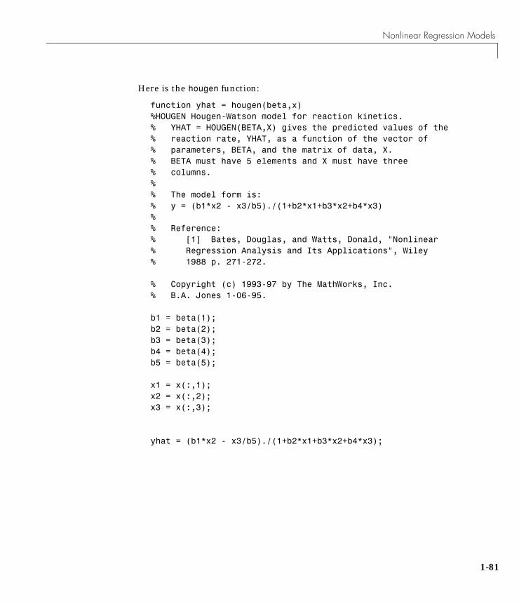
Nonlinear Regression Models
Here is the hougen function:
function yhat = hougen(beta,x)%HOUGEN Hougen-Watson model for reaction kinetics.% YHAT = HOUGEN(BETA,X) gives the predicted values of the% reaction rate, YHAT, as a function of the vector of % parameters, BETA, and the matrix of data, X.% BETA must have 5 elements and X must have three% columns.%% The model form is:% y = (b1*x2 - x3/b5)./(1+b2*x1+b3*x2+b4*x3)%% Reference:% [1] Bates, Douglas, and Watts, Donald, "Nonlinear% Regression Analysis and Its Applications", Wiley% 1988 p. 271-272.
% Copyright (c) 1993-97 by The MathWorks, Inc.% B.A. Jones 1-06-95.
b1 = beta(1);b2 = beta(2);b3 = beta(3);b4 = beta(4);b5 = beta(5);
x1 = x(:,1);x2 = x(:,2);x3 = x(:,3);
yhat = (b1*x2 - x3/b5)./(1+b2*x1+b3*x2+b4*x3);
1-81
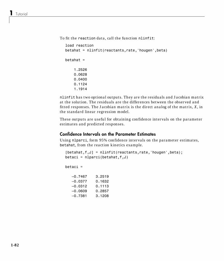
1 Tutorial
1-8
To fit the reaction data, call the function nlinfit:
load reactionbetahat = nlinfit(reactants,rate,'hougen',beta)
betahat =
1.2526 0.0628 0.0400 0.1124 1.1914
nlinfit has two optional outputs. They are the residuals and Jacobian matrixat the solution. The residuals are the differences between the observed andfitted responses. The Jacobian matrix is the direct analog of the matrix, X, inthe standard linear regression model.
These outputs are useful for obtaining confidence intervals on the parameterestimates and predicted responses.
Confidence Intervals on the Parameter EstimatesUsing nlparci, form 95% confidence intervals on the parameter estimates,betahat, from the reaction kinetics example.
[betahat,f,J] = nlinfit(reactants,rate,'hougen',beta);betaci = nlparci(betahat,f,J)
betaci =
–0.7467 3.2519 –0.0377 0.1632 –0.0312 0.1113 –0.0609 0.2857 –0.7381 3.1208
2
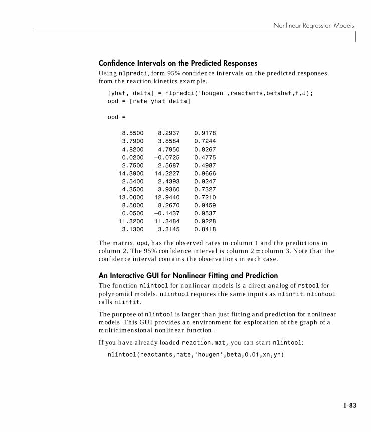
Nonlinear Regression Models
Confidence Intervals on the Predicted ResponsesUsing nlpredci, form 95% confidence intervals on the predicted responsesfrom the reaction kinetics example.
[yhat, delta] = nlpredci('hougen',reactants,betahat,f,J);opd = [rate yhat delta]
opd =
8.5500 8.2937 0.9178 3.7900 3.8584 0.7244 4.8200 4.7950 0.8267 0.0200 –0.0725 0.4775 2.7500 2.5687 0.4987 14.3900 14.2227 0.9666 2.5400 2.4393 0.9247 4.3500 3.9360 0.7327 13.0000 12.9440 0.7210 8.5000 8.2670 0.9459 0.0500 –0.1437 0.9537 11.3200 11.3484 0.9228 3.1300 3.3145 0.8418
The matrix, opd, has the observed rates in column 1 and the predictions incolumn 2. The 95% confidence interval is column 2 ± column 3. Note that theconfidence interval contains the observations in each case.
An Interactive GUI for Nonlinear Fitting and PredictionThe function nlintool for nonlinear models is a direct analog of rstool forpolynomial models. nlintool requires the same inputs as nlinfit. nlintoolcalls nlinfit.
The purpose of nlintool is larger than just fitting and prediction for nonlinearmodels. This GUI provides an environment for exploration of the graph of amultidimensional nonlinear function.
If you have already loaded reaction.mat, you can start nlintool:
nlintool(reactants,rate,'hougen',beta,0.01,xn,yn)
1-83
1 Tutorial
1-8
You will see a “vector” of three plots. The dependent variable of all three plotsis the reaction rate. The first plot has hydrogen as the independent variable.The second and third plots have n-pentane and isopentane respectively.
Each plot shows the fitted relationship of the reaction rate to the independentvariable at a fixed value of the other two independent variables. The fixedvalue of each independent variable is in an editable text box below each axis.You can change the fixed value of any independent variable by either typing anew value in the box or by dragging any of the 3 vertical lines to a new position.
When you change the value of an independent variable, all the plots update toshow the current picture at the new point in the space of the independentvariables.
Note that while this example only uses three reactants, nlintool, canaccommodate an arbitrary number of independent variables. Interpretabilitymay be limited by the size of the monitor for large numbers of inputs.
4
Hypothesis Tests
Hypothesis TestsA hypothesis test is a procedure for determining if an assertion about acharacteristic of a population is reasonable.
For example, suppose that someone says that the average price of a gallon ofregular unleaded gas in Massachusetts is $1.15. How would you decidewhether this statement is true? You could try to find out what every gas stationin the state was charging and how many gallons they were selling at that price.That approach might be definitive, but it could end up costing more than theinformation is worth.
A simpler approach is to find out the price of gas at a small number of randomlychosen stations around the state and compare the average price to $1.15.
Of course, the average price you get will probably not be exactly $1.15 due tovariability in price from one station to the next. Suppose your average pricewas $1.18. Is this three cent difference a result of chance variability, or is theoriginal assertion incorrect? A hypothesis test can provide an answer.
TerminologyTo get started, there are some terms to define and assumptions to make.
• The null hypothesis is the original assertion. In this case the null hypothesisis that the average price of a gallon of gas is $1.15. The notation is H0: µ =1.15.
• There are three possibilities for the alternative hypothesis. You might only beinterested in the result if gas prices were actually higher. In this case, thealternative hypothesis is H1: µ > 1.15. The other possibilities are H1: µ < 1.15and H1: µ ≠ 1.15.
• The significance level is related to the degree of certainty you require in orderto reject the null hypothesis in favor of the alternative. By taking a smallsample you cannot be certain about your conclusion. So you decide inadvance to reject the null hypothesis if the probability of observing yoursampled result is less than the significance level. For a typical significancelevel of 5% the notation is α = 0.05. For this significance level, the probabilityof incorrectly rejecting the null hypothesis when it is actually true is 5%. Ifyou need more protection from this error, then choose a lower value of α.
1-85
1 Tutorial
1-8
• The p-value is the probability of observing the given sample result under theassumption that the null hypothesis is true. If the p-value is less than α, thenyou reject the null hypothesis. For example, if α = 0.05 and the p-value is0.03, then you reject the null hypothesis.
The converse is not true. If the p-value is greater than α, you do not acceptthe null hypothesis. You just have insufficient evidence to reject the nullhypothesis (which is the same for practical purposes).
• The outputs for the hypothesis test functions also include confidenceintervals. Loosely speaking, a confidence interval is a range of values thathave a chosen probability of containing the true hypothesized quantity.Suppose, in our example, 1.15 is inside a 95% confidence interval for themean, µ. That is equivalent to being unable to reject the null hypothesis at asignificance level of 0.05. Conversely if the 100(1 – α) confidence intervaldoes not contain 1.15, then you reject the null hypothesis at the α level ofsignificance.
AssumptionsThe difference between hypothesis test procedures often arises fromdifferences in the assumptions that the researcher is willing to make about thedata sample. The Z-test assumes that the data represents independentsamples from the same normal distribution and that you know the standarddeviation, σ. The t-test has the same assumptions except that you estimate thestandard deviation using the data instead of specifying it as a known quantity.
Both tests have an associated signal-to-noise ratio:
The signal is the difference between the average and the hypothesized mean.The noise is the standard deviation posited or estimated.
If the null hypothesis is true, then Z has a standard normal distribution,N(0,1). T has a Student’s t distribution with the degrees of freedom, ν, equal toone less than the number of data values.
zx µ–
σ------------ or Tx µ–
s------------==
where xxin----
i 1=
n
∑=
6

Hypothesis Tests
Given the observed result for Z or T, and knowing their distribution assumingthe null hypothesis is true, it is possible to compute the probability (p-value) ofobserving this result. If the p-value is very small, then that casts doubt on thetruth of the null hypothesis. For example, suppose that the p-value was 0.001,meaning that the probability of observing the given Z (or T) was one in athousand. That should make you skeptical enough about the null hypothesisthat you reject it rather than believe that your result was just a lucky 999 to 1shot.
ExampleThis example uses the gasoline price data in gas.mat. There are two samplesof 20 observed gas prices for the months of January and February 1993.
load gasprices = [price1 price2]
prices =
119 118 117 115 115 115 116 122 112 118 121 121 115 120 122 122 116 120 118 113 109 120 112 123 119 121 112 109 117 117 113 117 114 120 109 116 109 118 118 125
1-87
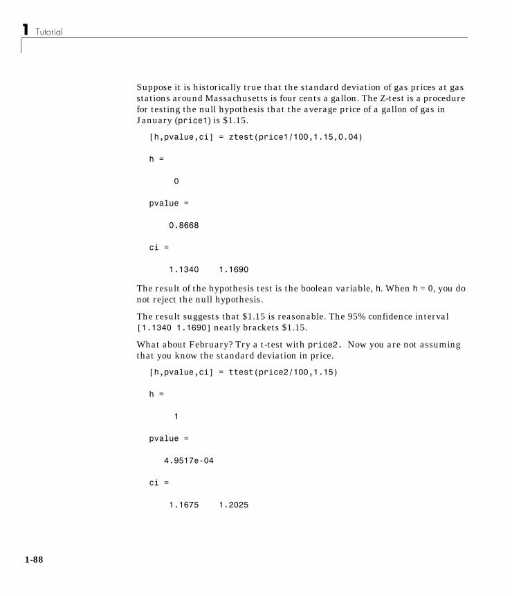
1 Tutorial
1-8
Suppose it is historically true that the standard deviation of gas prices at gasstations around Massachusetts is four cents a gallon. The Z-test is a procedurefor testing the null hypothesis that the average price of a gallon of gas inJanuary (price1) is $1.15.
[h,pvalue,ci] = ztest(price1/100,1.15,0.04)
h =
0
pvalue =
0.8668
ci =
1.1340 1.1690
The result of the hypothesis test is the boolean variable, h. When h = 0, you donot reject the null hypothesis.
The result suggests that $1.15 is reasonable. The 95% confidence interval[1.1340 1.1690] neatly brackets $1.15.
What about February? Try a t-test with price2. Now you are not assumingthat you know the standard deviation in price.
[h,pvalue,ci] = ttest(price2/100,1.15)
h =
1
pvalue =
4.9517e-04
ci =
1.1675 1.2025
8

Hypothesis Tests
With the boolean result, h = 1, you can reject the null hypothesis at the defaultsignificance level, 0.05.
It looks like $1.15 is not a reasonable estimate of the gasoline price inFebruary. The low end of the 95% confidence interval is greater than 1.15.
The function ttest2 allows you to compare the means of the two data samples.
[h,sig,ci] = ttest2(price1,price2)
h =
1
sig =
0.0083
ci =
–5.7845 –0.9155
The confidence interval (ci above) indicates that gasoline prices were betweenone and six cents lower in January than February.
1-89
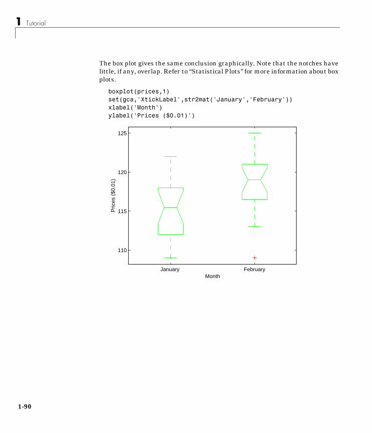
1 Tutorial
1-9
The box plot gives the same conclusion graphically. Note that the notches havelittle, if any, overlap. Refer to “Statistical Plots” for more information about boxplots.
boxplot(prices,1)set(gca,'XtickLabel',str2mat('January','February'))xlabel('Month')ylabel('Prices ($0.01)')
January February
110
115
120
125
Pric
es (
$0.0
1)
Month
0
Multivariate Statistics
Multivariate StatisticsMultivariate statistics is an omnibus term for a number of different statisticalmethods. The defining characteristic of these methods is that they all aim tounderstand a data set by considering a group of variables together rather thanfocusing on only one variable at a time.
Principal Components AnalysisOne of the difficulties inherent in multivariate statistics is the problem ofvisualizing multi-dimensionality. In MATLAB, the plot command displays agraph of the relationship between two variables. The plot3 and surfcommands display different three-dimensional views. When there are morethan three variables, it stretches the imagination to visualize theirrelationships.
Fortunately in data sets with many variables, groups of variables often movetogether. One reason for this is that more than one variable may be measuringthe same driving principle governing the behavior of the system. In manysystems there are only a few such driving forces. But an abundance ofinstrumentation allows us to measure dozens of system variables. When thishappens, we can take advantage of this redundancy of information. We cansimplify our problem by replacing a group of variables with a single newvariable.
Principal Components Analysis is a quantitatively rigorous method forachieving this simplification. The method generates a new set of variables,called principal components. Each principal component is a linear combinationof the original variables. All the principal components are orthogonal to eachother so there is no redundant information. The principal components as awhole form an orthogonal basis for the space of the data.
There are an infinite number of ways to construct an orthogonal basis forseveral columns of data. What is so special about the principal componentbasis?
The first principal component is a single axis in space. When you project eachobservation on that axis, the resulting values form a new variable. And thevariance of this variable is the maximum among all possible choices of the firstaxis.
1-91
1 Tutorial
1-9
The second principal component is another axis in space, perpendicular to thefirst. Projecting the observations on this axis generates another new variable.The variance of this variable is the maximum among all possible choices of thissecond axis.
The full set of principal components is as large as the original set of variables.But, it is commonplace for the sum of the variances of the first few principalcomponents to exceed 80% of the total variance of the original data. Byexamining plots of these few new variables, researchers often develop a deeperunderstanding of the driving forces that generated the original data.
ExampleLet us look at a sample application that uses nine different indices of thequality of life in 329 U.S. cities. These are climate, housing, health, crime,transportation, education, arts, recreation, and economics. For each index,higher is better; so, for example, a higher index for crime means a lower crimerate.
We start by loading the data in cities.mat.
load citieswhos Name Size Bytes Class
categories 9x14 252 char array names 329x43 28294 char array ratings 329x9 23688 double array
Grand total is 17234 elements using 52234 bytes
The whos command generates a table of information about all the variables inthe workspace. The cities data set contains three variables:
• categories, a string matrix containing the names of the indices.
• names, a string matrix containing the 329 city names.
• ratings, the data matrix with 329 rows and 9 columns.
2
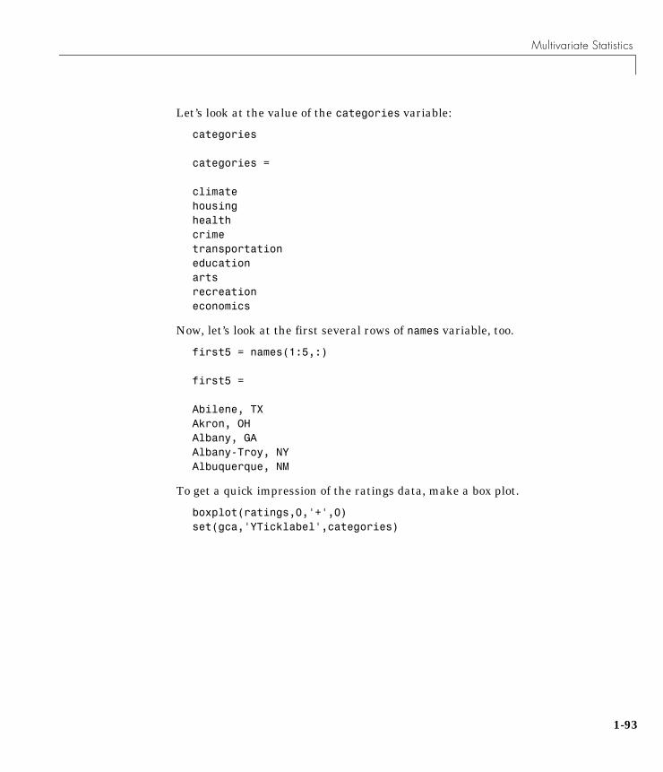
Multivariate Statistics
Let’s look at the value of the categories variable:
categories
categories =
climate housing health crime transportationeducation arts recreation economics
Now, let’s look at the first several rows of names variable, too.
first5 = names(1:5,:)
first5 =
Abilene, TX Akron, OH Albany, GA Albany-Troy, NY Albuquerque, NM
To get a quick impression of the ratings data, make a box plot.
boxplot(ratings,0,'+',0)set(gca,'YTicklabel',categories)
1-93
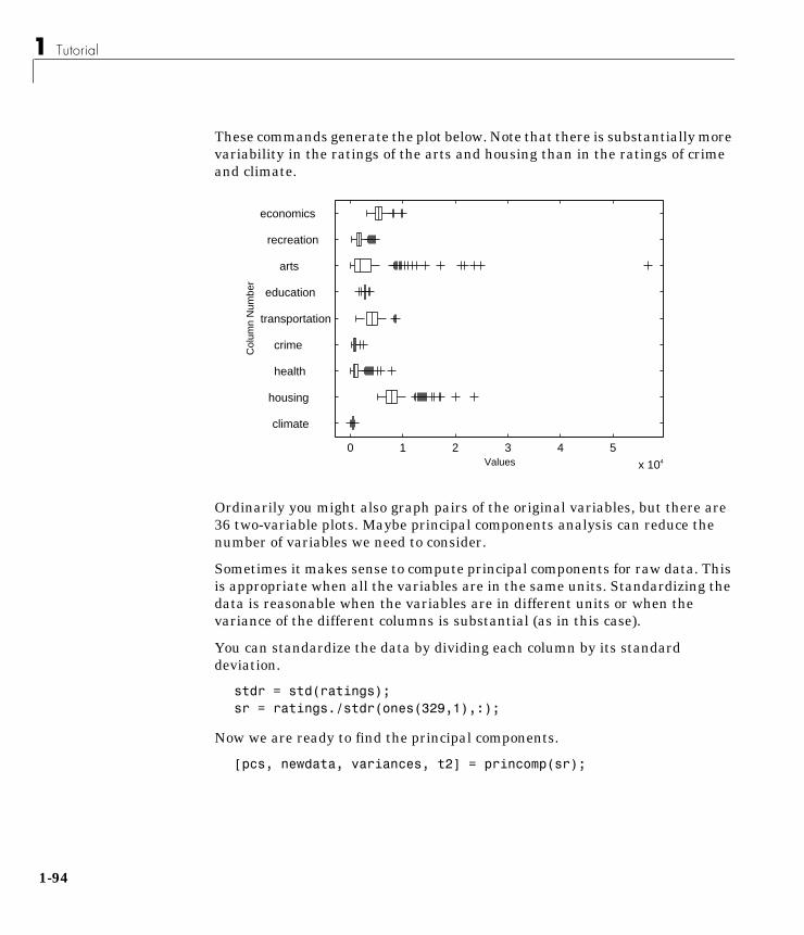
1 Tutorial
1-9
These commands generate the plot below. Note that there is substantially morevariability in the ratings of the arts and housing than in the ratings of crimeand climate.
Ordinarily you might also graph pairs of the original variables, but there are36 two-variable plots. Maybe principal components analysis can reduce thenumber of variables we need to consider.
Sometimes it makes sense to compute principal components for raw data. Thisis appropriate when all the variables are in the same units. Standardizing thedata is reasonable when the variables are in different units or when thevariance of the different columns is substantial (as in this case).
You can standardize the data by dividing each column by its standarddeviation.
stdr = std(ratings);sr = ratings./stdr(ones(329,1),:);
Now we are ready to find the principal components.
[pcs, newdata, variances, t2] = princomp(sr);
0 1 2 3 4 5
x 104
climate
housing
health
crime
transportation
education
arts
recreation
economics
Values
Col
umn
Num
ber
4
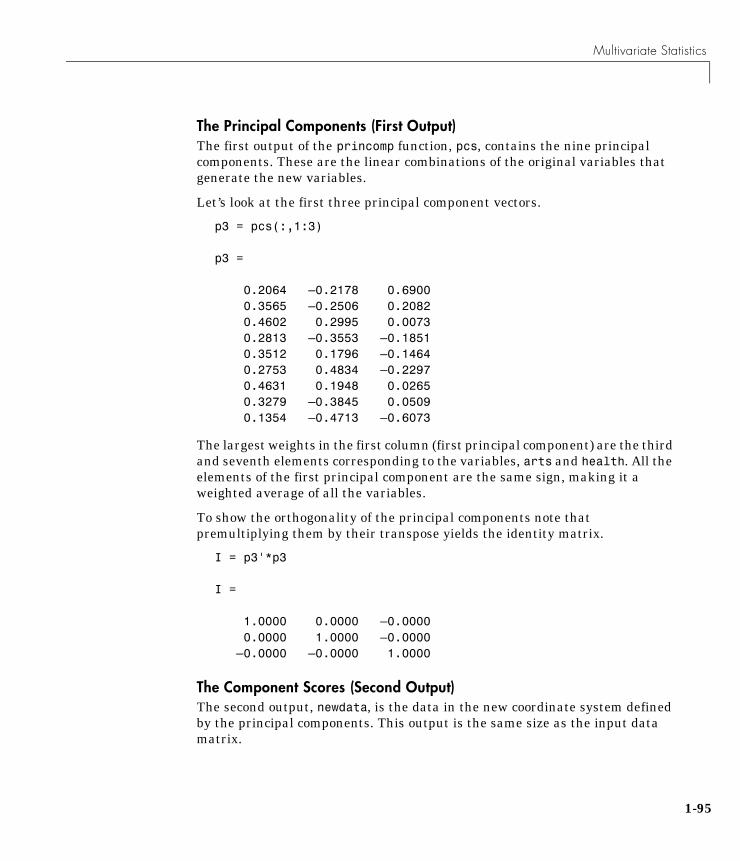
Multivariate Statistics
The Principal Components (First Output)The first output of the princomp function, pcs, contains the nine principalcomponents. These are the linear combinations of the original variables thatgenerate the new variables.
Let’s look at the first three principal component vectors.
p3 = pcs(:,1:3)
p3 =
0.2064 –0.2178 0.6900 0.3565 –0.2506 0.2082 0.4602 0.2995 0.0073 0.2813 –0.3553 –0.1851 0.3512 0.1796 –0.1464 0.2753 0.4834 –0.2297 0.4631 0.1948 0.0265 0.3279 –0.3845 0.0509 0.1354 –0.4713 –0.6073
The largest weights in the first column (first principal component) are the thirdand seventh elements corresponding to the variables, arts and health. All theelements of the first principal component are the same sign, making it aweighted average of all the variables.
To show the orthogonality of the principal components note thatpremultiplying them by their transpose yields the identity matrix.
I = p3'*p3
I =
1.0000 0.0000 –0.0000 0.0000 1.0000 –0.0000 –0.0000 –0.0000 1.0000
The Component Scores (Second Output)The second output, newdata, is the data in the new coordinate system definedby the principal components. This output is the same size as the input datamatrix.
1-95

1 Tutorial
1-9
A plot of the first two columns of newdata shows the ratings data projected ontothe first two principal components.
plot(newdata(:,1),newdata(:,2),'+')xlabel('1st Principal Component');ylabel('2nd Principal Component');
Note the outlying points in the upper right corner.
The function gname is useful for graphically identifying a few points in a plotlike this. You can call gname with a string matrix containing as many caselabels as points in the plot. The string matrix names works for labeling pointswith the city names.
gname(names)
Move your cursor over the plot and click once near each point at the top right.When you finish press the return key. Here is the resulting plot.
-4 -2 0 2 4 6 8 10 12 14-4
-3
-2
-1
0
1
2
3
4
1st Principal Component
2nd
Prin
cipa
l Com
pone
nt
6
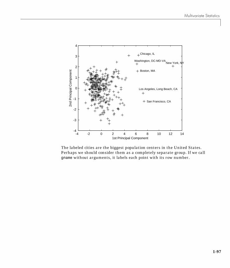
Multivariate Statistics
The labeled cities are the biggest population centers in the United States.Perhaps we should consider them as a completely separate group. If we callgname without arguments, it labels each point with its row number.
-4 -2 0 2 4 6 8 10 12 14-4
-3
-2
-1
0
1
2
3
4
1st Principal Component
2nd
Prin
cipa
l Com
pone
nt
Los Angeles, Long Beach, CA
San Francisco, CA
Boston, MA
Washington, DC-MD-VA
Chicago, IL
New York, NY
1-97

1 Tutorial
1-9
We can create an index variable containing the row numbers of all themetropolitan areas we chose.
metro = [43 65 179 213 234 270 314];names(metro,:)ans =
Boston, MA Chicago, IL Los Angeles, Long Beach, CA New York, NY Philadelphia, PA-NJ San Francisco, CA Washington, DC-MD-VA
-4 -2 0 2 4 6 8 10 12 14-4
-3
-2
-1
0
1
2
3
4
1st Principal Component
2nd
Prin
cipa
l Com
pone
nt
213
270
179
43
314
65234
8
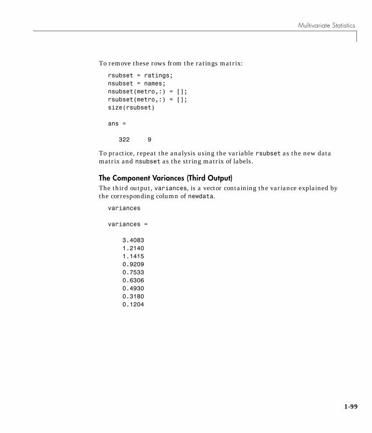
Multivariate Statistics
To remove these rows from the ratings matrix:
rsubset = ratings;nsubset = names;nsubset(metro,:) = [];rsubset(metro,:) = [];size(rsubset)
ans =
322 9
To practice, repeat the analysis using the variable rsubset as the new datamatrix and nsubset as the string matrix of labels.
The Component Variances (Third Output)The third output, variances, is a vector containing the variance explained bythe corresponding column of newdata.
variances
variances =
3.4083 1.2140 1.1415 0.9209 0.7533 0.6306 0.4930 0.3180 0.1204
1-99
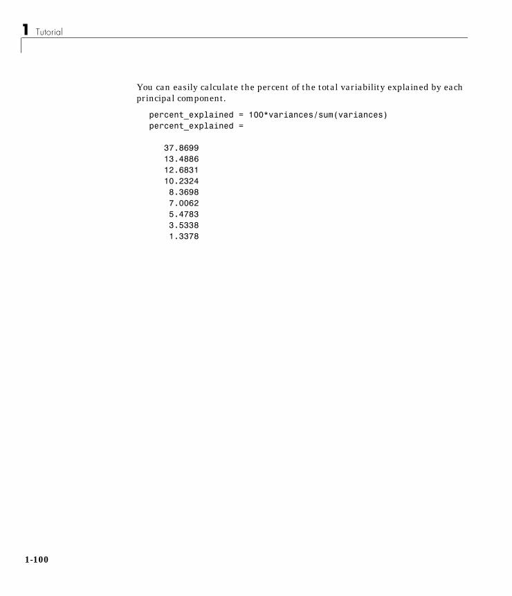
1 Tutorial
1-1
You can easily calculate the percent of the total variability explained by eachprincipal component.
percent_explained = 100*variances/sum(variances)percent_explained =
37.8699 13.4886 12.6831 10.2324 8.3698 7.0062 5.4783 3.5338 1.3378
00

Multivariate Statistics
A “Scree” plot is a pareto plot of the percent variability explained by eachprincipal component.
pareto(percent_explained)xlabel('Principal Component')ylabel('Variance Explained (%)')
We can see that the first three principal components explain roughly two thirdsof the total variability in the standardized ratings.
1 2 3 4 5 6 70
10
20
30
40
50
60
70
80
90
100
Principal Component
Var
ianc
e E
xpla
ined
(%
)
1-101

1 Tutorial
1-1
Hotelling’s T2 (Fourth Output)The last output of the princomp function, t2, is Hotelling’s T2, a statisticalmeasure of the multivariate distance of each observation from the center of thedata set. This is an analytical way to find the most extreme points in the data.
[st2, index] = sort(t2); % Sort in ascending order.st2 = flipud(st2); % Values in descending order.index = flipud(index); % Indices in descending order.extreme = index(1)
extreme =
213names(extreme,:)
ans =
New York, NY
It is not surprising that the ratings for New York are the furthest from theaverage U.S. town.
02
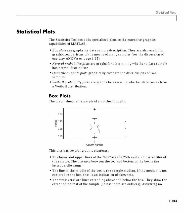
Statistical Plots
Statistical PlotsThe Statistics Toolbox adds specialized plots to the extensive graphicscapabilities of MATLAB.
• Box plots are graphs for data sample description. They are also useful forgraphic comparisons of the means of many samples (see the discussion ofone-way ANOVA on page 1-65).
• Normal probability plots are graphs for determining whether a data samplehas normal distribution.
• Quantile-quantile plots graphically compare the distributions of twosamples.
• Weibull probability plots are graphs for assessing whether data comes froma Weibull distribution.
Box PlotsThe graph shows an example of a notched box plot.
This plot has several graphic elements:
• The lower and upper lines of the “box” are the 25th and 75th percentiles ofthe sample. The distance between the top and bottom of the box is theinterquartile range.
• The line in the middle of the box is the sample median. If the median is notcentered in the box, that is an indication of skewness.
• The “whiskers” are lines extending above and below the box. They show theextent of the rest of the sample (unless there are outliers). Assuming no
1
110
115
120
125
Val
ues
Column Number
1-103
1 Tutorial
1-1
outliers, the maximum of the sample is the top of the upper whisker. Theminimum of the sample is the bottom of the lower whisker. By default, anoutlier is a value that is more than 1.5 times the interquartile range awayfrom the top or bottom of the box.
• The plus sign at the top of the plot is an indication of an outlier in the data.This point may be the result of a data entry error, a poor measurement or achange in the system that generated the data.
• The “notches” in the box are a graphic confidence interval about the medianof a sample. Box plots do not have notches by default.
A side-by-side comparison of two notched box plots is the graphical equivalentof a t-test. See the section “Hypothesis Tests” on page 1-85.
Normal Probability PlotsA normal probability plot is a useful graph for assessing whether data comesfrom a normal distribution. Many statistical procedures make the assumptionthat the underlying distribution of the data is normal, so this plot can providesome assurance that the assumption of normality is not being violated orprovide an early warning of a problem with your assumptions.
04
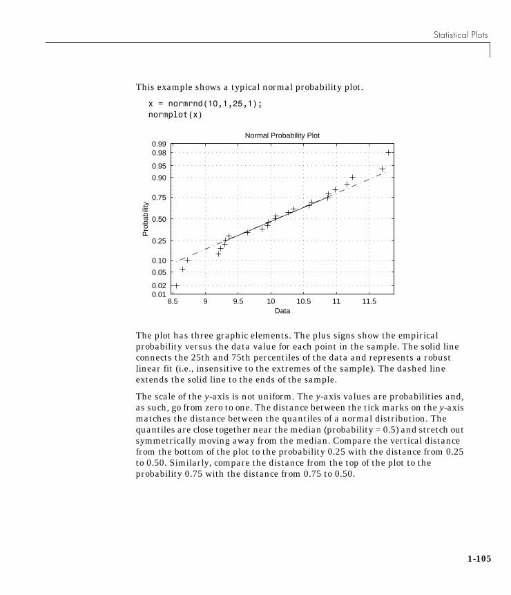
Statistical Plots
This example shows a typical normal probability plot.
x = normrnd(10,1,25,1);normplot(x)
The plot has three graphic elements. The plus signs show the empiricalprobability versus the data value for each point in the sample. The solid lineconnects the 25th and 75th percentiles of the data and represents a robustlinear fit (i.e., insensitive to the extremes of the sample). The dashed lineextends the solid line to the ends of the sample.
The scale of the y-axis is not uniform. The y-axis values are probabilities and,as such, go from zero to one. The distance between the tick marks on the y-axismatches the distance between the quantiles of a normal distribution. Thequantiles are close together near the median (probability = 0.5) and stretch outsymmetrically moving away from the median. Compare the vertical distancefrom the bottom of the plot to the probability 0.25 with the distance from 0.25to 0.50. Similarly, compare the distance from the top of the plot to theprobability 0.75 with the distance from 0.75 to 0.50.
8.5 9 9.5 10 10.5 11 11.50.01 0.02
0.05
0.10
0.25
0.50
0.75
0.90
0.95
0.98 0.99
Data
Pro
babi
lity
Normal Probability Plot
1-105
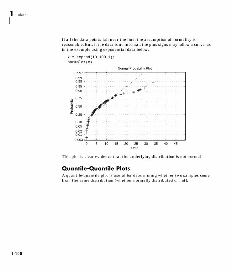
1 Tutorial
1-1
If all the data points fall near the line, the assumption of normality isreasonable. But, if the data is nonnormal, the plus signs may follow a curve, asin the example using exponential data below.
x = exprnd(10,100,1);normplot(x)
This plot is clear evidence that the underlying distribution is not normal.
Quantile-Quantile PlotsA quantile-quantile plot is useful for determining whether two samples comefrom the same distribution (whether normally distributed or not).
0 5 10 15 20 25 30 35 40 450.003
0.01 0.02
0.05 0.10
0.25
0.50
0.75
0.90 0.95
0.98 0.99
0.997
Data
Pro
babi
lity
Normal Probability Plot
06

Statistical Plots
The example shows a quantile-quantile plot of two samples from a Poissondistribution.
x = poissrnd(10,50,1);y = poissrnd(5,100,1);qqplot(x,y);
Even though the parameters and sample sizes are different, the straight linerelationship shows that the two samples come from the same distribution.
Like the normal probability plot, the quantile-quantile plot has three graphicelements. The pluses are the quantiles of each sample. By default the numberof pluses is the number of data values in the smaller sample. The solid line joinsthe 25th and 75th percentiles of the samples. The dashed line extends the solidline to the extent of the sample.
2 4 6 8 10 12 14 16 18-2
0
2
4
6
8
10
12
X Quantiles
Y Q
uant
iles
1-107
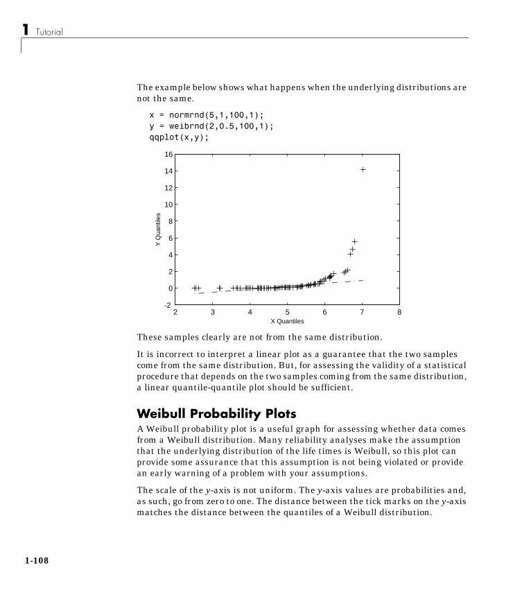
1 Tutorial
1-1
The example below shows what happens when the underlying distributions arenot the same.
x = normrnd(5,1,100,1);y = weibrnd(2,0.5,100,1);qqplot(x,y);
These samples clearly are not from the same distribution.
It is incorrect to interpret a linear plot as a guarantee that the two samplescome from the same distribution. But, for assessing the validity of a statisticalprocedure that depends on the two samples coming from the same distribution,a linear quantile-quantile plot should be sufficient.
Weibull Probability PlotsA Weibull probability plot is a useful graph for assessing whether data comesfrom a Weibull distribution. Many reliability analyses make the assumptionthat the underlying distribution of the life times is Weibull, so this plot canprovide some assurance that this assumption is not being violated or providean early warning of a problem with your assumptions.
The scale of the y-axis is not uniform. The y-axis values are probabilities and,as such, go from zero to one. The distance between the tick marks on the y-axismatches the distance between the quantiles of a Weibull distribution.
2 3 4 5 6 7 8-2
0
2
4
6
8
10
12
14
16
X Quantiles
Y Q
uant
iles
08
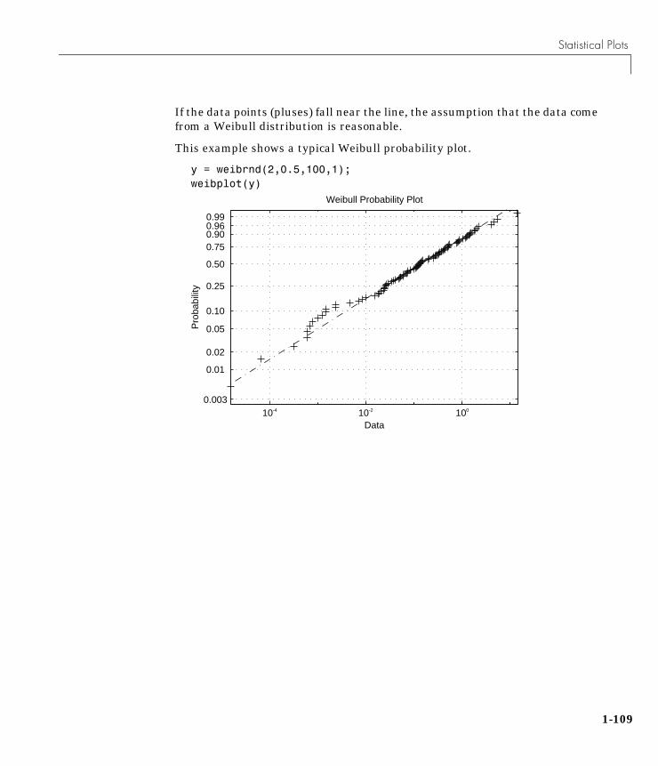
Statistical Plots
If the data points (pluses) fall near the line, the assumption that the data comefrom a Weibull distribution is reasonable.
This example shows a typical Weibull probability plot.
y = weibrnd(2,0.5,100,1);weibplot(y)
10-4 10-2 100
0.003
0.01
0.02
0.05
0.10
0.25
0.50
0.75 0.90 0.96 0.99
Data
Pro
babi
lity
Weibull Probability Plot
1-109
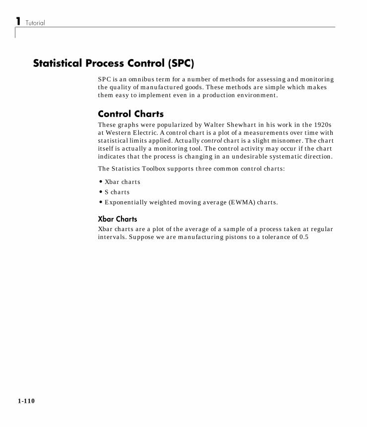
1 Tutorial
1-1
Statistical Process Control (SPC)SPC is an omnibus term for a number of methods for assessing and monitoringthe quality of manufactured goods. These methods are simple which makesthem easy to implement even in a production environment.
Control ChartsThese graphs were popularized by Walter Shewhart in his work in the 1920sat Western Electric. A control chart is a plot of a measurements over time withstatistical limits applied. Actually control chart is a slight misnomer. The chartitself is actually a monitoring tool. The control activity may occur if the chartindicates that the process is changing in an undesirable systematic direction.
The Statistics Toolbox supports three common control charts:
• Xbar charts
• S charts
• Exponentially weighted moving average (EWMA) charts.
Xbar ChartsXbar charts are a plot of the average of a sample of a process taken at regularintervals. Suppose we are manufacturing pistons to a tolerance of 0.5
10
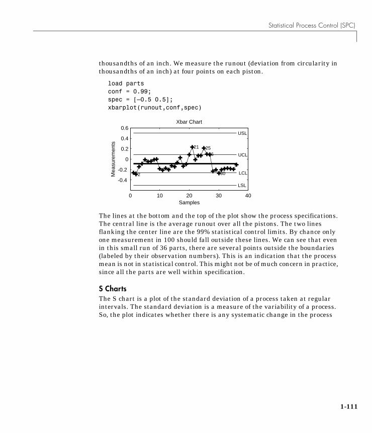
Statistical Process Control (SPC)
thousandths of an inch. We measure the runout (deviation from circularity inthousandths of an inch) at four points on each piston.
load partsconf = 0.99;spec = [–0.5 0.5];xbarplot(runout,conf,spec)
The lines at the bottom and the top of the plot show the process specifications.The central line is the average runout over all the pistons. The two linesflanking the center line are the 99% statistical control limits. By chance onlyone measurement in 100 should fall outside these lines. We can see that evenin this small run of 36 parts, there are several points outside the boundaries(labeled by their observation numbers). This is an indication that the processmean is not in statistical control. This might not be of much concern in practice,since all the parts are well within specification.
S ChartsThe S chart is a plot of the standard deviation of a process taken at regularintervals. The standard deviation is a measure of the variability of a process.So, the plot indicates whether there is any systematic change in the process
0 10 20 30 40
-0.4
-0.2
0
0.2
0.4
0.6
12
21 2526
30
Xbar Chart
USL
LSL
Samples
Mea
sure
men
ts
LCL
UCL
1-111
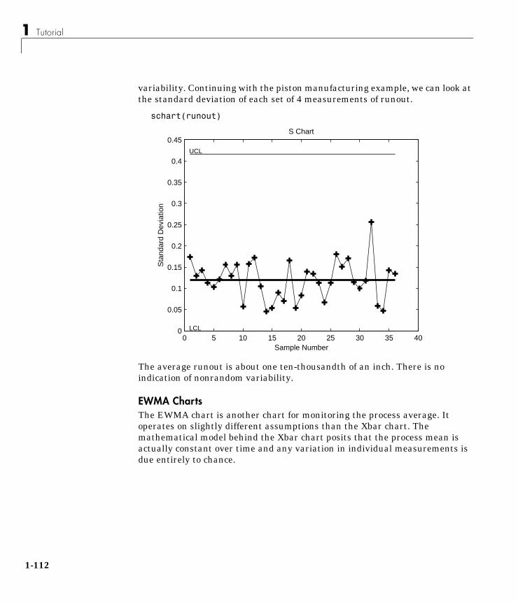
1 Tutorial
1-1
variability. Continuing with the piston manufacturing example, we can look atthe standard deviation of each set of 4 measurements of runout.
schart(runout)
The average runout is about one ten-thousandth of an inch. There is noindication of nonrandom variability.
EWMA ChartsThe EWMA chart is another chart for monitoring the process average. Itoperates on slightly different assumptions than the Xbar chart. Themathematical model behind the Xbar chart posits that the process mean isactually constant over time and any variation in individual measurements isdue entirely to chance.
0 5 10 15 20 25 30 35 400
0.05
0.1
0.15
0.2
0.25
0.3
0.35
0.4
0.45S Chart
Sample Number
Sta
ndar
d D
evia
tion
UCL
LCL
12
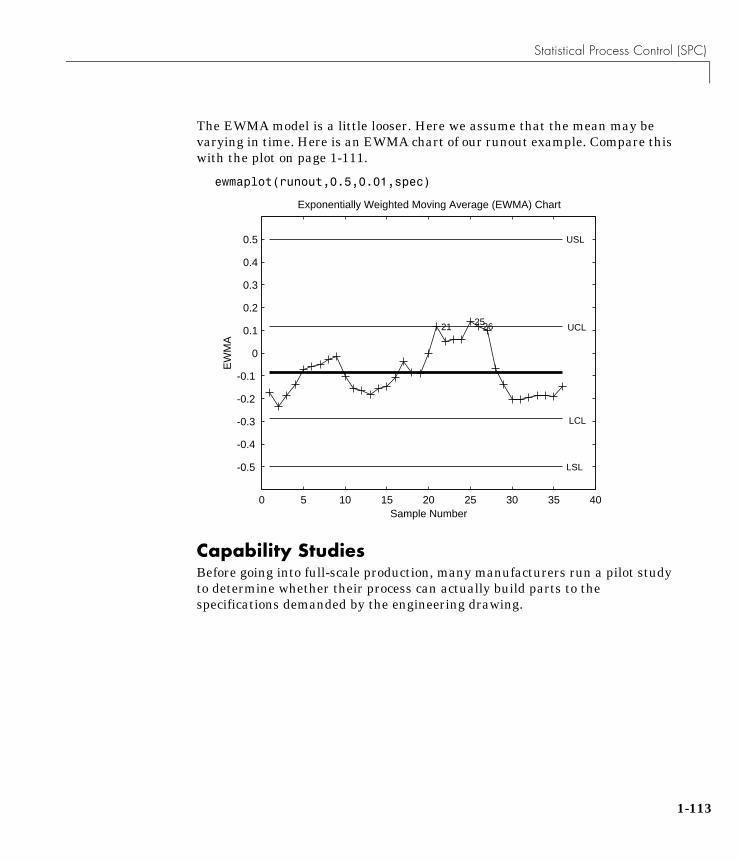
Statistical Process Control (SPC)
The EWMA model is a little looser. Here we assume that the mean may bevarying in time. Here is an EWMA chart of our runout example. Compare thiswith the plot on page 1-111.
ewmaplot(runout,0.5,0.01,spec)
Capability StudiesBefore going into full-scale production, many manufacturers run a pilot studyto determine whether their process can actually build parts to thespecifications demanded by the engineering drawing.
0 5 10 15 20 25 30 35 40
-0.5
-0.4
-0.3
-0.2
-0.1
0
0.1
0.2
0.3
0.4
0.5
21 2526
Exponentially Weighted Moving Average (EWMA) Chart
USL
LSL
Sample Number
EW
MA
UCL
LCL
1-113

1 Tutorial
1-1
Using the data from these capability studies with a statistical model allows usto get a preliminary estimate of the percentage of parts that will fall outsidethe specifications.
[p, Cp, Cpk] = capable(mean(runout),spec)
p =
1.3940e–09
Cp =
2.3950
Cpk =
1.9812
The result above shows that the probability (p = 1.3940e–09) of observing anunacceptable runout is extremely low. Cp and Cpk are two popular capabilityindices.
Cp is the ratio of the range of the specifications to six times the estimate of theprocess standard deviation.
For a process that has its average value on target, a Cp of one translates to alittle more than one defect per thousand. Recently many industries have set aquality goal of one part per million. This would correspond to a Cp = 1.6. Thehigher the value of Cp the more capable the process.
Cpk is the ratio of difference between the process mean and the closerspecification limit to three times the estimate of the process standarddeviation.
where the process mean is µ. For processes that do not maintain their averageon target, Cpk, is a more descriptive index of process capability.
CpUSL LSL–
6σ--------------------------------=
Cpk minUSL µ–
3σ-----------------------µ LSL–
3σ----------------------, =
14
Design of Experiments (DOE)
Design of Experiments (DOE)There is a world of difference between data and information. To extractinformation from data you have to make assumptions about the system thatgenerated the data. Using these assumptions and physical theory you may beable to develop a mathematical model of the system.
Generally, even rigorously formulated models have some unknown constants.The goal of experimentation is to acquire data that allow us to estimate theseconstants.
But why do we need to experiment at all? We could instrument the system wewant to study and just let it run. Sooner or later we would have all the data wecould use.
In fact, this is a fairly common approach. There are three characteristics ofhistorical data that pose problems for statistical modeling:
• Suppose we observe a change in the operating variables of a system followedby a change in the outputs of the system. That does not necessarily meanthat the change in the system caused the change in the outputs.
• A common assumption in statistical modeling is that the observations areindependent of each other. This is not the way a system in normal operationworks.
• Controlling a system in operation often means changing system variables intandem. But if two variables change together, it is impossible to separatetheir effects mathematically.
Designed experiments directly address these problems. The overwhelmingadvantage of a designed experiment is that you actively manipulate the systemyou are studying.
With DOE you may generate fewer data points than by using passiveinstrumentation, but the quality of the information you get will be higher.
The Statistics Toolbox provides several functions for generating experimentaldesigns appropriate to various situations.
1-115

1 Tutorial
1-1
Full Factorial DesignsSuppose you want to determine whether the variability of a machining processis due to the difference in the lathes that cut the parts or the operators who runthe lathes.
If the same operator always runs a given lathe then you cannot tell whetherthe machine or the operator is the cause of the variation in the output. Byallowing every operator to run every lathe you can separate their effects.
This is a factorial approach. fullfact is the function that generates the design.Suppose we have four operators and three machines. What is the factorialdesign?
d = fullfact([4 3])
d =
1 1 2 1 3 1 4 1 1 2 2 2 3 2 4 2 1 3 2 3 3 3 4 3
Each row of d represents one operator/machine combination. Note that thereare 4*3 = 12 rows.
16
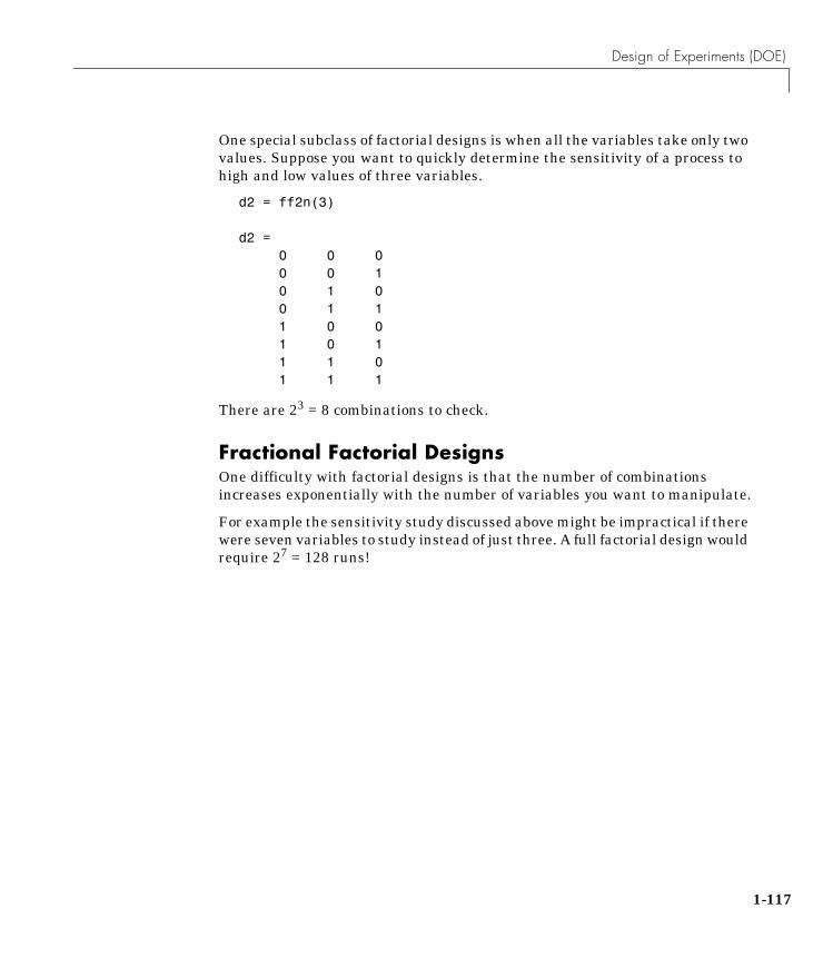
Design of Experiments (DOE)
One special subclass of factorial designs is when all the variables take only twovalues. Suppose you want to quickly determine the sensitivity of a process tohigh and low values of three variables.
d2 = ff2n(3)
d2 = 0 0 0 0 0 1 0 1 0 0 1 1 1 0 0 1 0 1 1 1 0 1 1 1
There are 23 = 8 combinations to check.
Fractional Factorial DesignsOne difficulty with factorial designs is that the number of combinationsincreases exponentially with the number of variables you want to manipulate.
For example the sensitivity study discussed above might be impractical if therewere seven variables to study instead of just three. A full factorial design wouldrequire 27 = 128 runs!
1-117
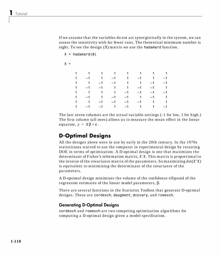
1 Tutorial
1-1
If we assume that the variables do not act synergistically in the system, we canassess the sensitivity with far fewer runs. The theoretical minimum number iseight. To see the design (X) matrix we use the hadamard function.
X = hadamard(8)
X =
1 1 1 1 1 1 1 1 1 –1 1 –1 1 –1 1 –1 1 1 –1 –1 1 1 –1 –1 1 –1 –1 1 1 –1 –1 1 1 1 1 1 –1 –1 –1 –1 1 –1 1 –1 –1 1 –1 1 1 1 –1 –1 –1 –1 1 1 1 –1 –1 1 –1 1 1 –1
The last seven columns are the actual variable settings (–1 for low, 1 for high.)The first column (all ones) allows us to measure the mean effect in the linearequation, .
D-Optimal DesignsAll the designs above were in use by early in the 20th century. In the 1970sstatisticians started to use the computer in experimental design by recastingDOE in terms of optimization. A D-optimal design is one that maximizes thedeterminant of Fisher’s information matrix, X'X. This matrix is proportional tothe inverse of the covariance matrix of the parameters. So maximizing det(X'X)is equivalent to minimizing the determinant of the covariance of theparameters.
A D-optimal design minimizes the volume of the confidence ellipsoid of theregression estimates of the linear model parameters, β.
There are several functions in the Statistics Toolbox that generate D-optimaldesigns. These are cordexch, daugment, dcovary, and rowexch.
Generating D-Optimal Designscordexch and rowexch are two competing optimization algorithms forcomputing a D-optimal design given a model specification.
y Xβ ε+=
18
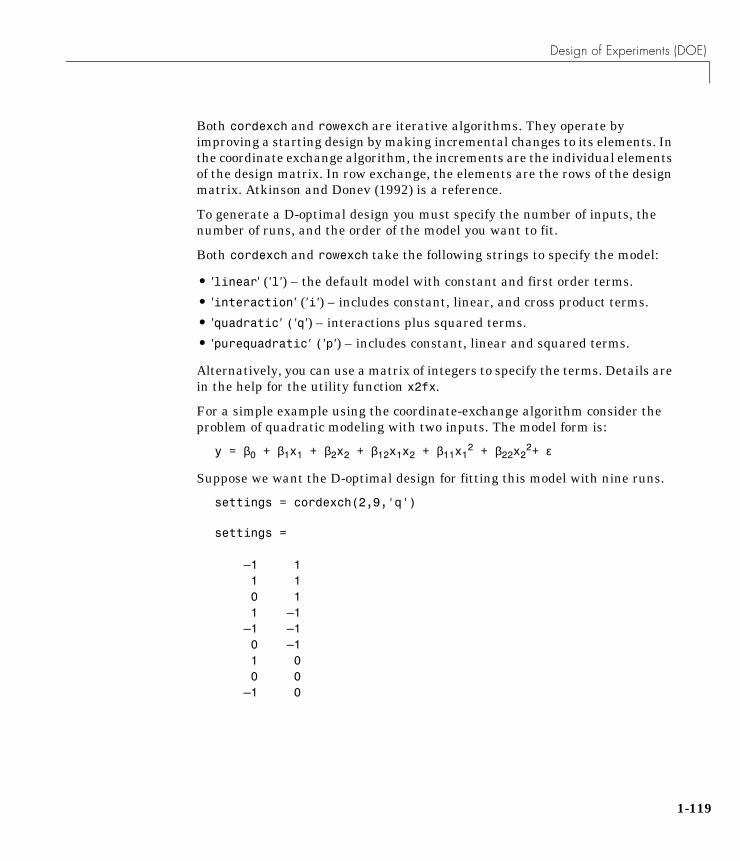
Design of Experiments (DOE)
Both cordexch and rowexch are iterative algorithms. They operate byimproving a starting design by making incremental changes to its elements. Inthe coordinate exchange algorithm, the increments are the individual elementsof the design matrix. In row exchange, the elements are the rows of the designmatrix. Atkinson and Donev (1992) is a reference.
To generate a D-optimal design you must specify the number of inputs, thenumber of runs, and the order of the model you want to fit.
Both cordexch and rowexch take the following strings to specify the model:
• 'linear' ('l') – the default model with constant and first order terms.
• 'interaction' ('i') – includes constant, linear, and cross product terms.
• 'quadratic' ('q') – interactions plus squared terms.
• 'purequadratic' ('p') – includes constant, linear and squared terms.
Alternatively, you can use a matrix of integers to specify the terms. Details arein the help for the utility function x2fx.
For a simple example using the coordinate-exchange algorithm consider theproblem of quadratic modeling with two inputs. The model form is:
y = β0 + β1x1 + β2x2 + β12x1x2 + β11x12 + β22x2
2+ ε
Suppose we want the D-optimal design for fitting this model with nine runs.
settings = cordexch(2,9,'q')
settings =
–1 1 1 1 0 1 1 –1 –1 –1 0 –1 1 0 0 0 –1 0
1-119

1 Tutorial
1-1
We can plot the columns of settings against each other to get a better pictureof the design.
h = plot(settings(:,1),settings(:,2),'.');set(gca,'Xtick',[-1 0 1])set(gca,'Ytick',[-1 0 1])set(h,'Markersize',20)
For a simple example using the row-exchange algorithm, consider theinteraction model with two inputs. The model form is:
y = β0 + β1x1 + β2x2 + β12x1x2 + ε
Suppose we want the D-optimal design for fitting this model with four runs.
[settings, X] = rowexch(2,4,'i')
settings =
–1 1 –1 –1 1 –1 1 1
X =
1 –1 1 –1 1 –1 –1 1 1 1 –1 –1 1 1 1 1
-1 0 1-1
0
1
20

Design of Experiments (DOE)
The settings matrix shows how to vary the inputs from run to run. The X matrixis the design matrix for fitting the above regression model. The first column ofX is for fitting the constant term. The last column is the element-wise productof the second and third columns.
The associated plot is simple but elegant.
h = plot(settings(:,1),settings(:,2),'.');set(gca,'Xtick',[-1 0 1])set(gca,'Ytick',[-1 0 1])set(h,'Markersize',20)
Augmenting D-Optimal DesignsIn practice, experimentation is an iterative process. We often want to add runsto a completed experiment to learn more about our system. The functiondaugment allows you choose these extra runs optimally.
-1 0 1-1
0
1
1-121
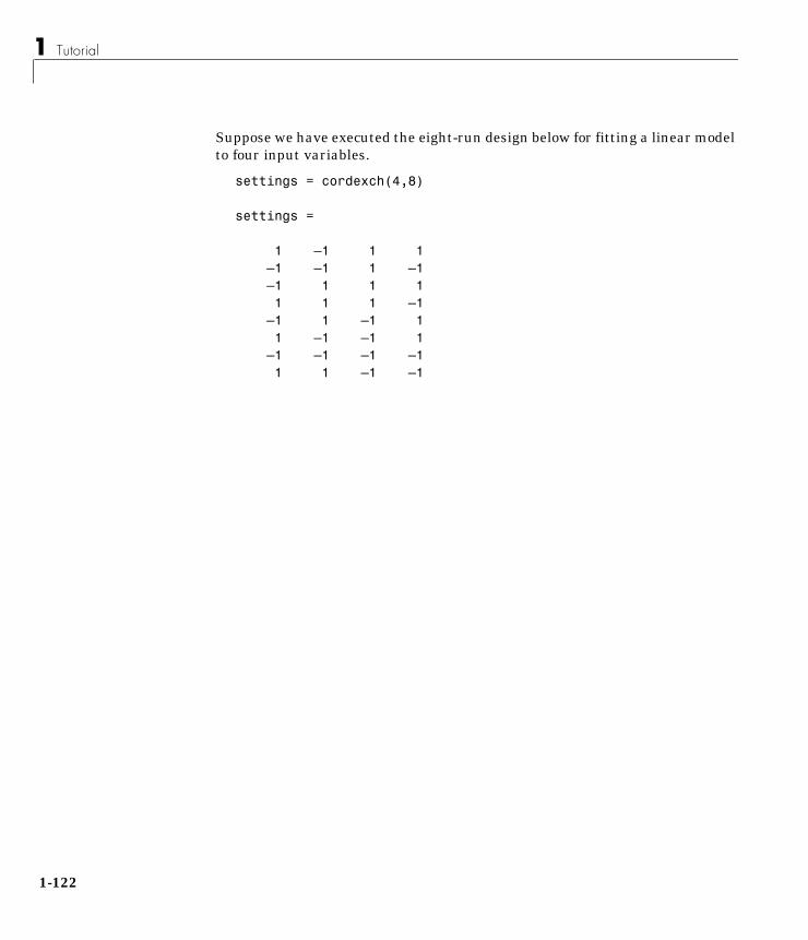
1 Tutorial
1-1
Suppose we have executed the eight-run design below for fitting a linear modelto four input variables.
settings = cordexch(4,8)
settings =
1 –1 1 1 –1 –1 1 –1 –1 1 1 1 1 1 1 –1 –1 1 –1 1 1 –1 –1 1 –1 –1 –1 –1 1 1 –1 –1
22

Design of Experiments (DOE)
This design is adequate to fit the linear model for four inputs, but cannot fit thesix cross-product (interaction) terms. Suppose we are willing to do eight moreruns to fit these extra terms. Here’s how.
[augmented, X] = daugment(settings,8,'i');augmented
augmented =
1 –1 1 1 –1 –1 1 –1 –1 1 1 1 1 1 1 –1 –1 1 –1 1 1 –1 –1 1 –1 –1 –1 –1 1 1 –1 –1 –1 –1 –1 1 1 1 1 1 –1 –1 1 1 –1 1 1 –1 1 –1 1 –1 1 –1 –1 –1 –1 1 –1 –1 1 1 –1 1info = X'*X
info =
16 0 0 0 0 0 0 0 0 0 0 0 16 0 0 0 0 0 0 0 0 0 0 0 16 0 0 0 0 0 0 0 0 0 0 0 16 0 0 0 0 0 0 0 0 0 0 0 16 0 0 0 0 0 0 0 0 0 0 0 16 0 0 0 0 0 0 0 0 0 0 0 16 0 0 0 0 0 0 0 0 0 0 0 16 0 0 0 0 0 0 0 0 0 0 0 16 0 0 0 0 0 0 0 0 0 0 0 16 0 0 0 0 0 0 0 0 0 0 0 16
1-123
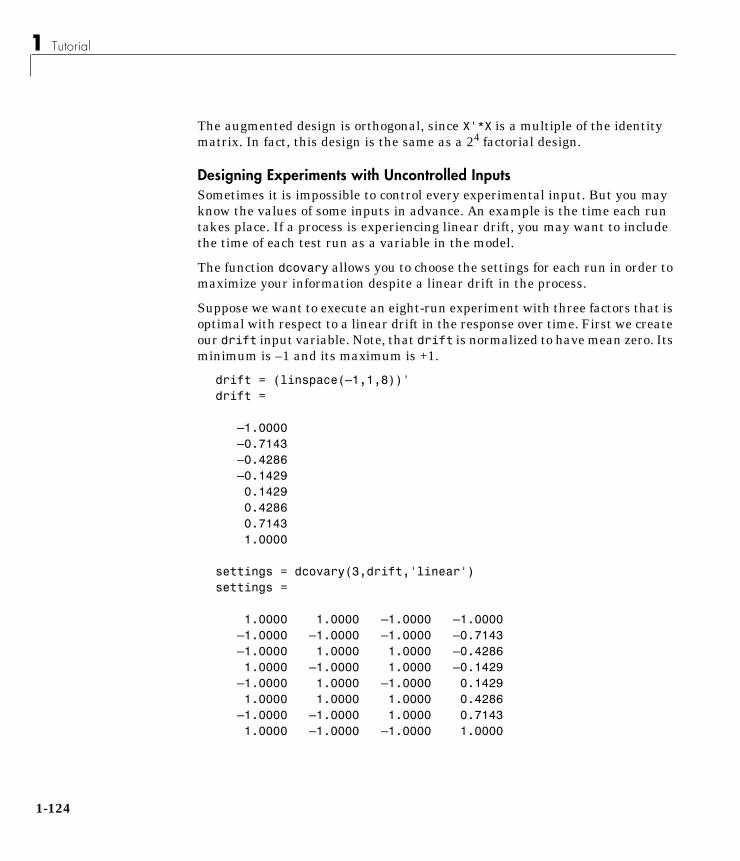
1 Tutorial
1-1
The augmented design is orthogonal, since X'*X is a multiple of the identitymatrix. In fact, this design is the same as a 24 factorial design.
Designing Experiments with Uncontrolled InputsSometimes it is impossible to control every experimental input. But you mayknow the values of some inputs in advance. An example is the time each runtakes place. If a process is experiencing linear drift, you may want to includethe time of each test run as a variable in the model.
The function dcovary allows you to choose the settings for each run in order tomaximize your information despite a linear drift in the process.
Suppose we want to execute an eight-run experiment with three factors that isoptimal with respect to a linear drift in the response over time. First we createour drift input variable. Note, that drift is normalized to have mean zero. Itsminimum is –1 and its maximum is +1.
drift = (linspace(–1,1,8))'drift =
–1.0000 –0.7143 –0.4286 –0.1429 0.1429 0.4286 0.7143 1.0000
settings = dcovary(3,drift,'linear')settings =
1.0000 1.0000 –1.0000 –1.0000 –1.0000 –1.0000 –1.0000 –0.7143 –1.0000 1.0000 1.0000 –0.4286 1.0000 –1.0000 1.0000 –0.1429 –1.0000 1.0000 –1.0000 0.1429 1.0000 1.0000 1.0000 0.4286 –1.0000 –1.0000 1.0000 0.7143 1.0000 –1.0000 –1.0000 1.0000
24
Demos
DemosThe Statistics Toolbox has demonstration programs that create an interactiveenvironment for exploring the probability distribution, random numbergeneration, curve fitting, and design of experiments functions.
The disttool Demo disttool is a graphic environment for developing an intuitive understandingof probability distributions.
The disttool demo has the following features:
• A graph of the cdf (pdf) for the given parameters of a distribution.
• A pop-up menu for changing the distribution function.
• A pop-up menu for changing the function type (cdf <–> pdf).
• Sliders to change the parameter settings.
• Data entry boxes to choose specific parameter values.
• Data entry boxes to change the limits of the parameter sliders.
• Draggable horizontal and vertical reference lines to do interactive evaluationof the function at varying values.
• A data entry box to evaluate the function at a specific x-value.
• For cdf plots, a data entry box on the probability axis (y-axis) to find criticalvalues corresponding to a specific probability.
• A Close button to end the demonstration.
Demo Purpose
disttool Graphic interaction with probability distributions.
polytool Interactive graphic prediction of polynomial fits.
randtool Interactive control of random number generation.
rsmdemo Design of Experiments and regression modeling.
1-125
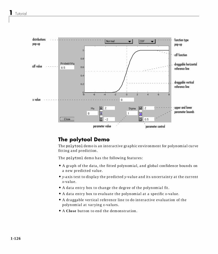
1 Tutorial
1-1
The polytool DemoThe polytool demo is an interactive graphic environment for polynomial curvefitting and prediction.
The polytool demo has the following features:
• A graph of the data, the fitted polynomial, and global confidence bounds ona new predicted value.
• y-axis text to display the predicted y-value and its uncertainty at the currentx-value.
• A data entry box to change the degree of the polynomial fit.
• A data entry box to evaluate the polynomial at a specific x-value.
• A draggable vertical reference line to do interactive evaluation of thepolynomial at varying x-values.
• A Close button to end the demonstration.
-8 -6 -4 -2 0 2 4 6 80
0.2
0.4
0.6
0.8
1
function type pop-up
cdf function
draggable vertical reference line
parameter value
distributions pop-up
cdf value
x value
parameter control
draggable horizontal reference line
upper and lower parameter bounds
26

Demos
You can use polytool to do curve fitting and prediction for any set of x-y data,but, for the sake of demonstration, the Statistics Toolbox provides a dataset(polydata.mat) to teach some basic concepts.
To start the demonstration you must first load the dataset.
load polydatawhoYour variables are:
x x1 y y1
The variables x and y are observations made with error from a cubicpolynomial. The variables x1 and y1 are data points from the “true” functionwithout error.
If you do not specify the degree of the polynomial, polytool does a linear fit tothe data.
polytool(x,y)
0 1 2 3 4 5 6 7 8 9 103
4
5
6
7
8
9
10
11
12
13
predicted value
box for controlling polynomial degree
95% confidence interval
draggable reference line
lower confidence bound
fitted line
upper confidence bound
x-value
data point
1-127
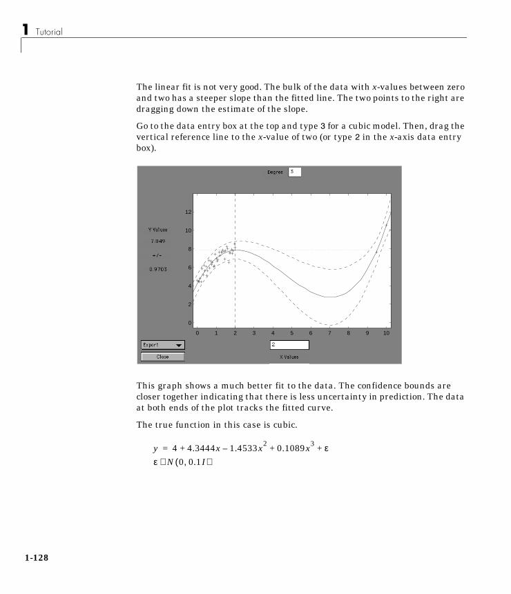
1 Tutorial
1-1
The linear fit is not very good. The bulk of the data with x-values between zeroand two has a steeper slope than the fitted line. The two points to the right aredragging down the estimate of the slope.
Go to the data entry box at the top and type 3 for a cubic model. Then, drag thevertical reference line to the x-value of two (or type 2 in the x-axis data entrybox).
This graph shows a much better fit to the data. The confidence bounds arecloser together indicating that there is less uncertainty in prediction. The dataat both ends of the plot tracks the fitted curve.
The true function in this case is cubic.
0 1 2 3 4 5 6 7 8 9 10
0
2
4
6
8
10
12
y 4 4.3444x 1.4533x2– 0.1089x3 ε+ + +=
ε N 0 0.1I,( )∼
28
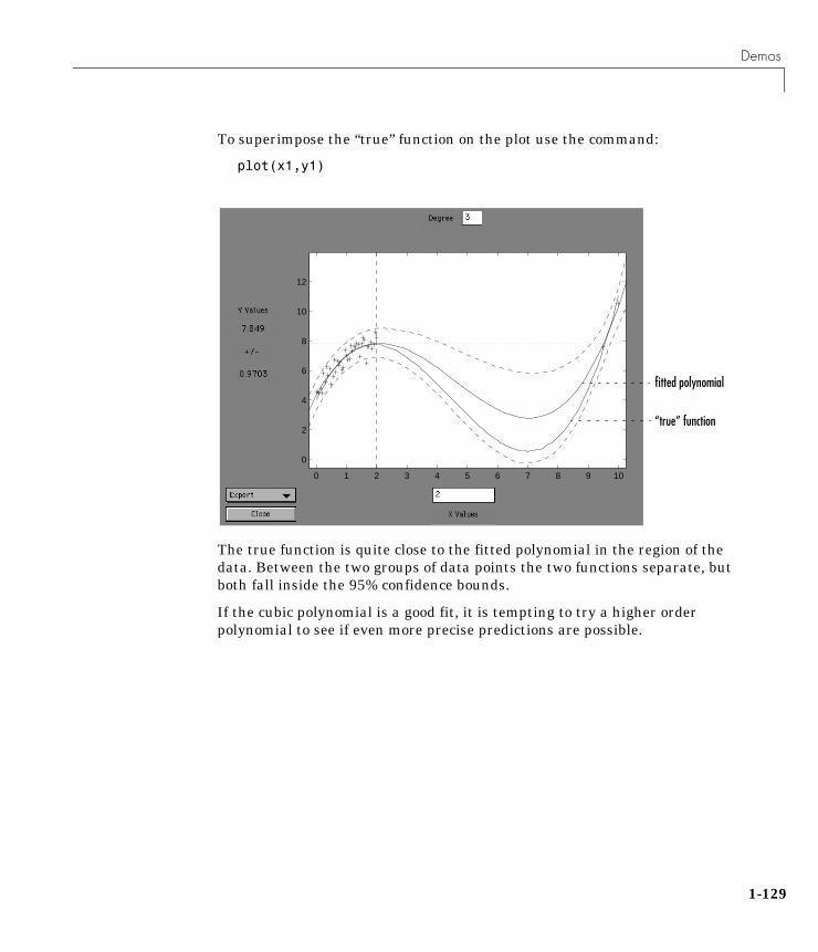
Demos
To superimpose the “true” function on the plot use the command:
plot(x1,y1)
The true function is quite close to the fitted polynomial in the region of thedata. Between the two groups of data points the two functions separate, butboth fall inside the 95% confidence bounds.
If the cubic polynomial is a good fit, it is tempting to try a higher orderpolynomial to see if even more precise predictions are possible.
0 1 2 3 4 5 6 7 8 9 10
0
2
4
6
8
10
12
“true” function
fitted polynomial
1-129
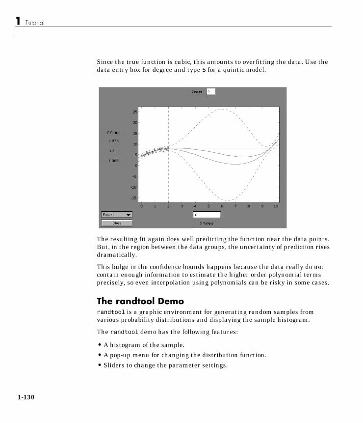
1 Tutorial
1-1
Since the true function is cubic, this amounts to overfitting the data. Use thedata entry box for degree and type 5 for a quintic model.
The resulting fit again does well predicting the function near the data points.But, in the region between the data groups, the uncertainty of prediction risesdramatically.
This bulge in the confidence bounds happens because the data really do notcontain enough information to estimate the higher order polynomial termsprecisely, so even interpolation using polynomials can be risky in some cases.
The randtool Demorandtool is a graphic environment for generating random samples fromvarious probability distributions and displaying the sample histogram.
The randtool demo has the following features:
• A histogram of the sample.
• A pop-up menu for changing the distribution function.
• Sliders to change the parameter settings.
0 1 2 3 4 5 6 7 8 9 10
-15
-10
-5
0
5
10
15
20
25
30
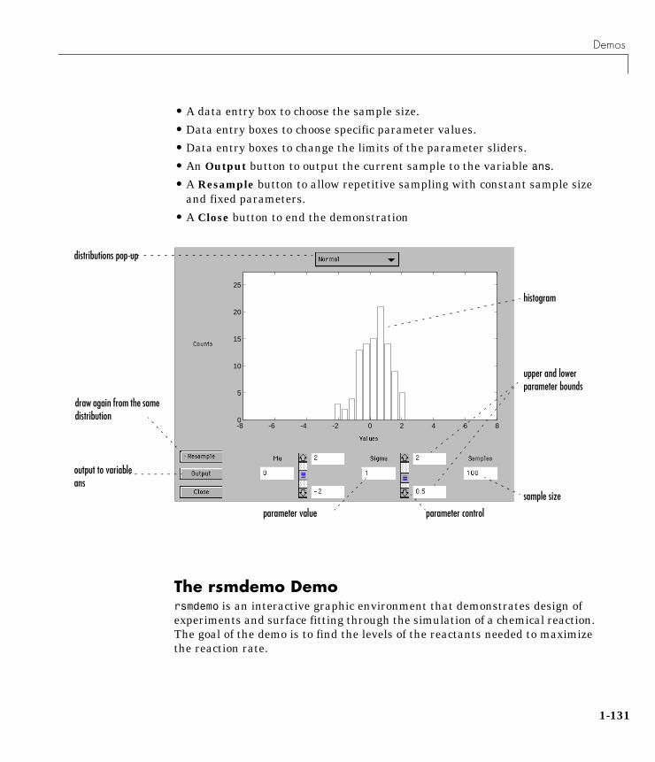
Demos
• A data entry box to choose the sample size.
• Data entry boxes to choose specific parameter values.
• Data entry boxes to change the limits of the parameter sliders.
• An Output button to output the current sample to the variable ans.
• A Resample button to allow repetitive sampling with constant sample sizeand fixed parameters.
• A Close button to end the demonstration
The rsmdemo Demo rsmdemo is an interactive graphic environment that demonstrates design ofexperiments and surface fitting through the simulation of a chemical reaction.The goal of the demo is to find the levels of the reactants needed to maximizethe reaction rate.
-8 -6 -4 -2 0 2 4 6 80
5
10
15
20
25
parameter value
draw again from the same distribution
output to variable ans
parameter control
histogram
upper and lower parameter bounds
sample size
distributions pop-up
1-131
1 Tutorial
1-1
There are two parts to the demo:
1 Compare data gathered through trial and error with data from a designedexperiment.
2 Compare response surface (polynomial) modeling with nonlinear modeling.
Part 1Begin the demo by using the sliders in the Reaction Simulator to control thepartial pressures of three reactants: Hydrogen, n-Pentane, and Isopentane.Each time you click the Run button, the levels for the reactants and results ofthe run are entered in the Trial and Error Data window.
Based on the results of previous runs, you can change the levels of thereactants to increase the reaction rate. (The results are determined using anunderlying model that takes into account the noise in the process, so even if youkeep all of the levels the same, the results will vary from run to run.) You areallotted a budget of 13 runs. When you have completed the runs, you can usethe Plot menu on the Trial and Error Data window to plot the relationshipsbetween the reactants and the reaction rate, or click the Analyze button. Whenyou click Analyze, rsmdemo calls the rstool function, which you can then useto try to optimize the results.)
Next, perform another set of 13 runs, this time from a designed experiment. Inthe Experimental Design Data window, click the Do Experiment button.rsmdemo calls the cordexch function to generate a D-optimal design, and then,for each run, computes the reaction rate.
Now use the Plot menu on the Experimental Design Data window to plot therelationships between the levels of the reactants and the reaction rate, or clickthe Response Surface button to call rstool to find the optimal levels of thereactants.
Compare the analysis results for the two sets of data. It is likely (though notcertain) that you’ll find some or all of these differences:
• You can fit a full quadratic model with the data from the designedexperiment, but the trial and error data may be insufficient for fitting aquadratic model or interactions model.
• Using the data from the designed experiment, you are more likely to be ableto find levels for the reactants that result in the maximum reaction rate.
32

Demos
Even if you find the best settings using the trial and error data, theconfidence bounds are likely to be wider than those from the designedexperiment.
Part 2Now analyze the experimental design data with a polynomial model and anonlinear model, and comparing the results. The true model for the process,which is used to generate the data, is actually a nonlinear model. However,within the range of the data, a quadratic model approximates the true modelquite well.
To see the polynomial model, click the Response Surface button on theExperimental Design Data window. rsmdemo calls rstool, which fits a fullquadratic model to the data. Drag the reference lines to change the levels of thereactants, and find the optimal reaction rate. Observe the width of theconfidence intervals.
Now click the Nonlinear Model button on the Experimental Design Datawindow. rsmdemo calls nlintool, which fits a Hougen-Watson model to thedata. As with the quadratic model, you can drag the reference lines to changethe reactant levels. Observe the reaction rate and the confidence intervals.
Compare the analysis results for the two models. Even though the true modelis nonlinear, you may find that the polynomial model provides a good fit.Because polynomial models are much easier to fit and work with thannonlinear models, a polynomial model is often preferable even when modelinga nonlinear process. Keep in mind, however, that such models are unlikely tobe reliable for extrapolating outside the range of the data.
1-133
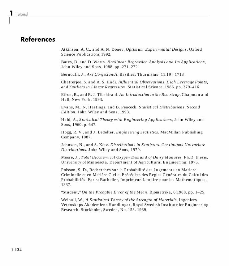
1 Tutorial
1-1
ReferencesAtkinson, A. C., and A. N. Donev, Optimum Experimental Designs, OxfordScience Publications 1992.
Bates, D. and D. Watts. Nonlinear Regression Analysis and Its Applications,John Wiley and Sons. 1988. pp. 271–272.
Bernoulli, J., Ars Conjectandi, Basiliea: Thurnisius [11.19], 1713
Chatterjee, S. and A. S. Hadi. Influential Observations, High Leverage Points,and Outliers in Linear Regression. Statistical Science, 1986. pp. 379–416.
Efron, B., and R. J. Tibshirani. An Introduction to the Bootstrap, Chapman andHall, New York. 1993.
Evans, M., N. Hastings, and B. Peacock. Statistical Distributions, SecondEdition. John Wiley and Sons, 1993.
Hald, A., Statistical Theory with Engineering Applications, John Wiley andSons, 1960. p. 647.
Hogg, R. V., and J. Ledolter. Engineering Statistics. MacMillan PublishingCompany, 1987.
Johnson, N., and S. Kotz. Distributions in Statistics: Continuous UnivariateDistributions. John Wiley and Sons, 1970.
Moore, J., Total Biochemical Oxygen Demand of Dairy Manures. Ph.D. thesis.University of Minnesota, Department of Agricultural Engineering, 1975.
Poisson, S. D., Recherches sur la Probabilité des Jugements en MatiereCriminelle et en Metière Civile, Précédées des Regles Générales du Calcul desProbabilitiés. Paris: Bachelier, Imprimeur-Libraire pour les Mathematiques,1837.
“Student,” On the Probable Error of the Mean. Biometrika, 6:1908. pp. 1–25.
Weibull, W., A Statistical Theory of the Strength of Materials. IngeniorsVetenskaps Akademiens Handlingar, Royal Swedish Institute for EngineeringResearch. Stockholm, Sweden, No. 153. 1939.
34

2
Reference
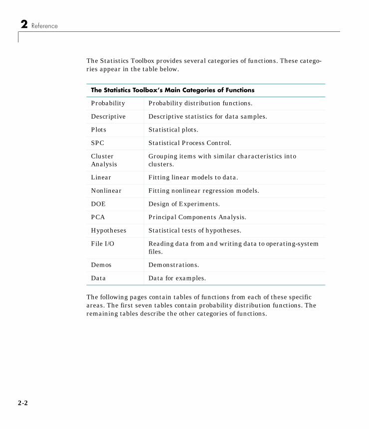
2 Reference
The Statistics Toolbox provides several categories of functions. These catego-ries appear in the table below.
The following pages contain tables of functions from each of these specificareas. The first seven tables contain probability distribution functions. Theremaining tables describe the other categories of functions.
The Statistics Toolbox’s Main Categories of Functions
Probability Probability distribution functions.
Descriptive Descriptive statistics for data samples.
Plots Statistical plots.
SPC Statistical Process Control.
ClusterAnalysis
Grouping items with similar characteristics intoclusters.
Linear Fitting linear models to data.
Nonlinear Fitting nonlinear regression models.
DOE Design of Experiments.
PCA Principal Components Analysis.
Hypotheses Statistical tests of hypotheses.
File I/O Reading data from and writing data to operating-systemfiles.
Demos Demonstrations.
Data Data for examples.
2-2
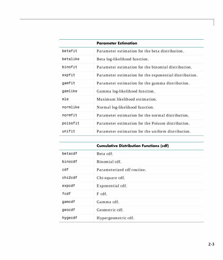
Parameter Estimation
betafit Parameter estimation for the beta distribution.
betalike Beta log-likelihood function.
binofit Parameter estimation for the binomial distribution.
expfit Parameter estimation for the exponential distribution.
gamfit Parameter estimation for the gamma distribution.
gamlike Gamma log-likelihood function.
mle Maximum likelihood estimation.
normlike Normal log-likelihood function.
normfit Parameter estimation for the normal distribution.
poissfit Parameter estimation for the Poisson distribution.
unifit Parameter estimation for the uniform distribution.
Cumulative Distribution Functions (cdf)
betacdf Beta cdf.
binocdf Binomial cdf.
cdf Parameterized cdf routine.
chi2cdf Chi-square cdf.
expcdf Exponential cdf.
fcdf F cdf.
gamcdf Gamma cdf.
geocdf Geometric cdf.
hygecdf Hypergeometric cdf.
2-3

2 Reference
logncdf Lognormal cdf.
nbincdf Negative binomial cdf.
ncfcdf Noncentral F cdf.
nctcdf Noncentral t cdf.
ncx2cdf Noncentral Chi-square cdf.
normcdf Normal (Gaussian) cdf.
poisscdf Poisson cdf.
raylcdf Rayleigh cdf.
tcdf Student’s t cdf.
unidcdf Discrete uniform cdf.
unifcdf Continuous uniform cdf.
weibcdf Weibull cdf.
Probability Density Functions (pdf)
betapdf Beta pdf.
binopdf Binomial pdf.
chi2pdf Chi-square pdf.
exppdf Exponential pdf.
fpdf F pdf.
gampdf Gamma pdf.
geopdf Geometric pdf.
hygepdf Hypergeometric pdf.
Cumulative Distribution Functions (cdf) (Continued)
2-4

normpdf Normal (Gaussian) pdf.
lognpdf Lognormal pdf.
nbinpdf Negative binomial pdf.
ncfpdf Noncentral F pdf.
nctpdf Noncentral t pdf.
ncx2pdf Noncentral Chi-square pdf.
pdf Parameterized pdf routine.
poisspdf Poisson pdf.
raylpdf Rayleigh pdf.
tpdf Student’s t pdf.
unidpdf Discrete uniform pdf.
unifpdf Continuous uniform pdf.
weibpdf Weibull pdf.
Inverse Cumulative Distribution Functions
betainv Beta critical values.
binoinv Binomial critical values.
chi2inv Chi-square critical values.
expinv Exponential critical values.
finv F critical values.
gaminv Gamma critical values.
geoinv Geometric critical values.
Probability Density Functions (pdf) (Continued)
2-5
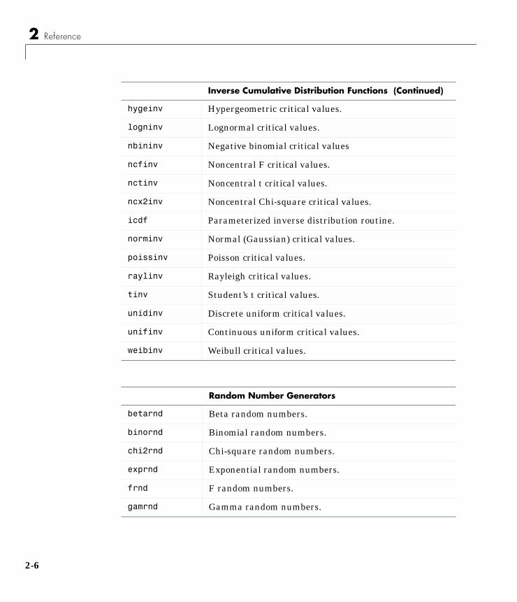
2 Reference
hygeinv Hypergeometric critical values.
logninv Lognormal critical values.
nbininv Negative binomial critical values
ncfinv Noncentral F critical values.
nctinv Noncentral t critical values.
ncx2inv Noncentral Chi-square critical values.
icdf Parameterized inverse distribution routine.
norminv Normal (Gaussian) critical values.
poissinv Poisson critical values.
raylinv Rayleigh critical values.
tinv Student’s t critical values.
unidinv Discrete uniform critical values.
unifinv Continuous uniform critical values.
weibinv Weibull critical values.
Random Number Generators
betarnd Beta random numbers.
binornd Binomial random numbers.
chi2rnd Chi-square random numbers.
exprnd Exponential random numbers.
frnd F random numbers.
gamrnd Gamma random numbers.
Inverse Cumulative Distribution Functions (Continued)
2-6
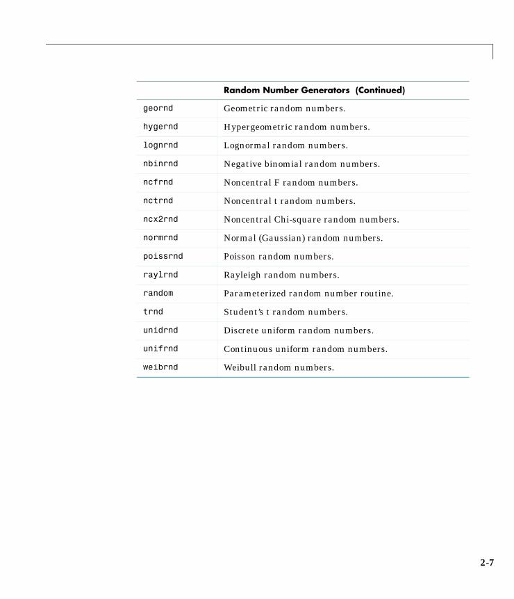
geornd Geometric random numbers.
hygernd Hypergeometric random numbers.
lognrnd Lognormal random numbers.
nbinrnd Negative binomial random numbers.
ncfrnd Noncentral F random numbers.
nctrnd Noncentral t random numbers.
ncx2rnd Noncentral Chi-square random numbers.
normrnd Normal (Gaussian) random numbers.
poissrnd Poisson random numbers.
raylrnd Rayleigh random numbers.
random Parameterized random number routine.
trnd Student’s t random numbers.
unidrnd Discrete uniform random numbers.
unifrnd Continuous uniform random numbers.
weibrnd Weibull random numbers.
Random Number Generators (Continued)
2-7
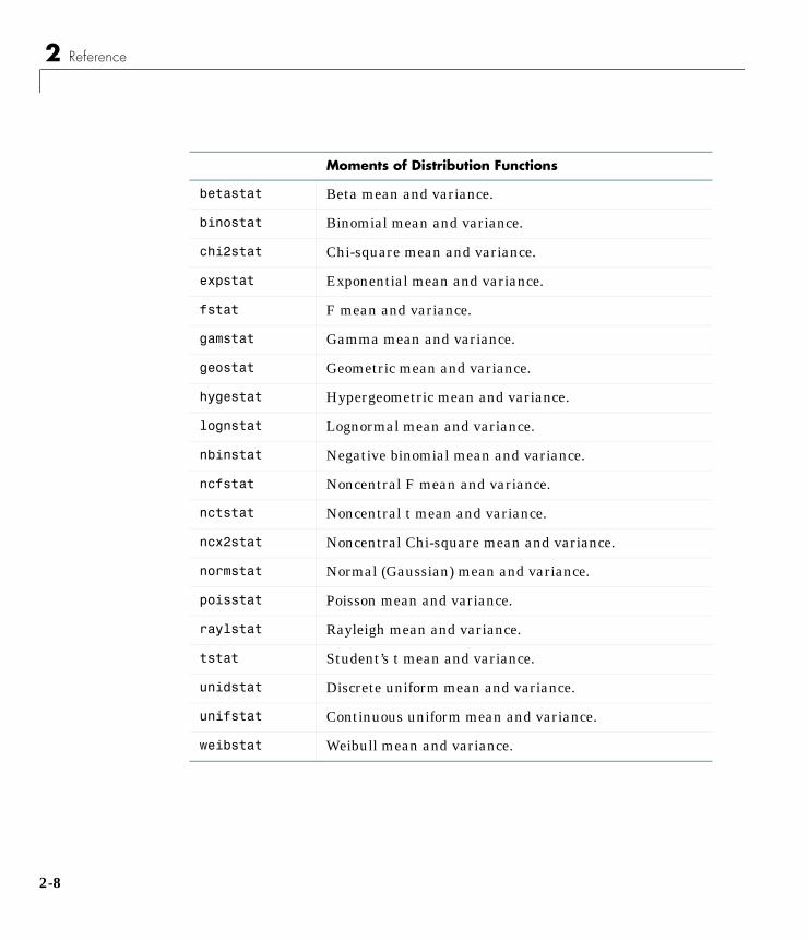
2 Reference
Moments of Distribution Functions
betastat Beta mean and variance.
binostat Binomial mean and variance.
chi2stat Chi-square mean and variance.
expstat Exponential mean and variance.
fstat F mean and variance.
gamstat Gamma mean and variance.
geostat Geometric mean and variance.
hygestat Hypergeometric mean and variance.
lognstat Lognormal mean and variance.
nbinstat Negative binomial mean and variance.
ncfstat Noncentral F mean and variance.
nctstat Noncentral t mean and variance.
ncx2stat Noncentral Chi-square mean and variance.
normstat Normal (Gaussian) mean and variance.
poisstat Poisson mean and variance.
raylstat Rayleigh mean and variance.
tstat Student’s t mean and variance.
unidstat Discrete uniform mean and variance.
unifstat Continuous uniform mean and variance.
weibstat Weibull mean and variance.
2-8

Descriptive Statistics
corrcoef Correlation coefficients (in MATLAB).
cov Covariance matrix (in MATLAB).
geomean Geometric mean.
harmmean Harmonic mean.
iqr Interquartile range.
kurtosis Sample kurtosis.
mad Mean absolute deviation.
mean Arithmetic average (in MATLAB).
median 50th percentile (in MATLAB).
moment Central moments of all orders.
nanmax Maximum ignoring missing data.
nanmean Average ignoring missing data.
nanmedian Median ignoring missing data.
nanmin Minimum ignoring missing data.
nanstd Standard deviation ignoring missing data.
nansum Sum ignoring missing data.
prctile Empirical percentiles of a sample.
range Sample range.
skewness Sample skewness.
std Standard deviation (in MATLAB).
trimmean Trimmed mean.
var Variance.
2-9
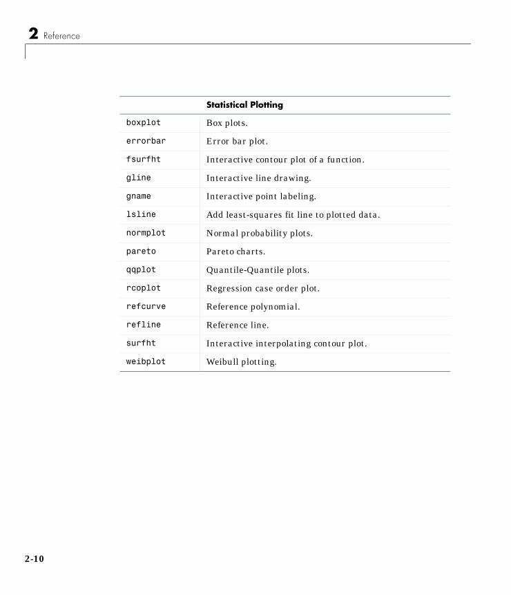
2 Reference
Statistical Plotting
boxplot Box plots.
errorbar Error bar plot.
fsurfht Interactive contour plot of a function.
gline Interactive line drawing.
gname Interactive point labeling.
lsline Add least-squares fit line to plotted data.
normplot Normal probability plots.
pareto Pareto charts.
qqplot Quantile-Quantile plots.
rcoplot Regression case order plot.
refcurve Reference polynomial.
refline Reference line.
surfht Interactive interpolating contour plot.
weibplot Weibull plotting.
2-10
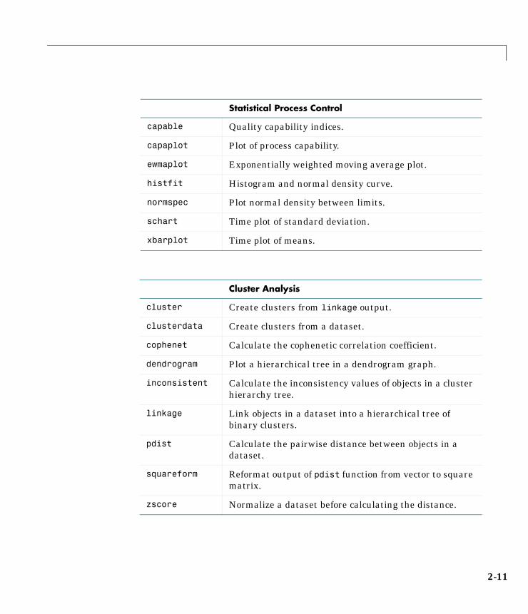
Statistical Process Control
capable Quality capability indices.
capaplot Plot of process capability.
ewmaplot Exponentially weighted moving average plot.
histfit Histogram and normal density curve.
normspec Plot normal density between limits.
schart Time plot of standard deviation.
xbarplot Time plot of means.
Cluster Analysis
cluster Create clusters from linkage output.
clusterdata Create clusters from a dataset.
cophenet Calculate the cophenetic correlation coefficient.
dendrogram Plot a hierarchical tree in a dendrogram graph.
inconsistent Calculate the inconsistency values of objects in a clusterhierarchy tree.
linkage Link objects in a dataset into a hierarchical tree ofbinary clusters.
pdist Calculate the pairwise distance between objects in adataset.
squareform Reformat output of pdist function from vector to squarematrix.
zscore Normalize a dataset before calculating the distance.
2-11
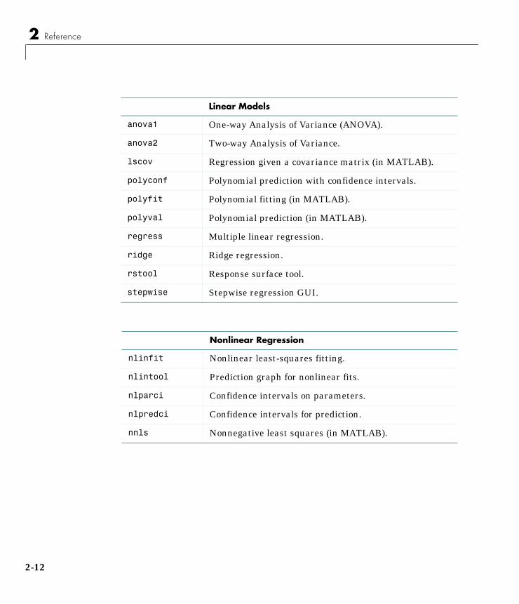
2 Reference
Linear Models
anova1 One-way Analysis of Variance (ANOVA).
anova2 Two-way Analysis of Variance.
lscov Regression given a covariance matrix (in MATLAB).
polyconf Polynomial prediction with confidence intervals.
polyfit Polynomial fitting (in MATLAB).
polyval Polynomial prediction (in MATLAB).
regress Multiple linear regression.
ridge Ridge regression.
rstool Response surface tool.
stepwise Stepwise regression GUI.
Nonlinear Regression
nlinfit Nonlinear least-squares fitting.
nlintool Prediction graph for nonlinear fits.
nlparci Confidence intervals on parameters.
nlpredci Confidence intervals for prediction.
nnls Nonnegative least squares (in MATLAB).
2-12
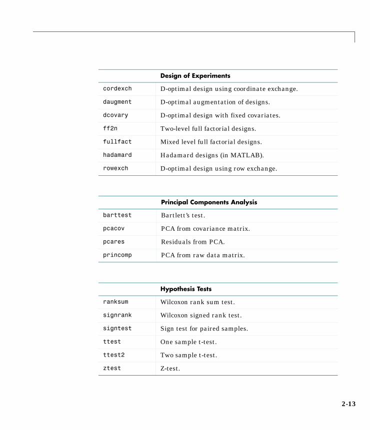
Design of Experiments
cordexch D-optimal design using coordinate exchange.
daugment D-optimal augmentation of designs.
dcovary D-optimal design with fixed covariates.
ff2n Two-level full factorial designs.
fullfact Mixed level full factorial designs.
hadamard Hadamard designs (in MATLAB).
rowexch D-optimal design using row exchange.
Principal Components Analysis
barttest Bartlett’s test.
pcacov PCA from covariance matrix.
pcares Residuals from PCA.
princomp PCA from raw data matrix.
Hypothesis Tests
ranksum Wilcoxon rank sum test.
signrank Wilcoxon signed rank test.
signtest Sign test for paired samples.
ttest One sample t-test.
ttest2 Two sample t-test.
ztest Z-test.
2-13
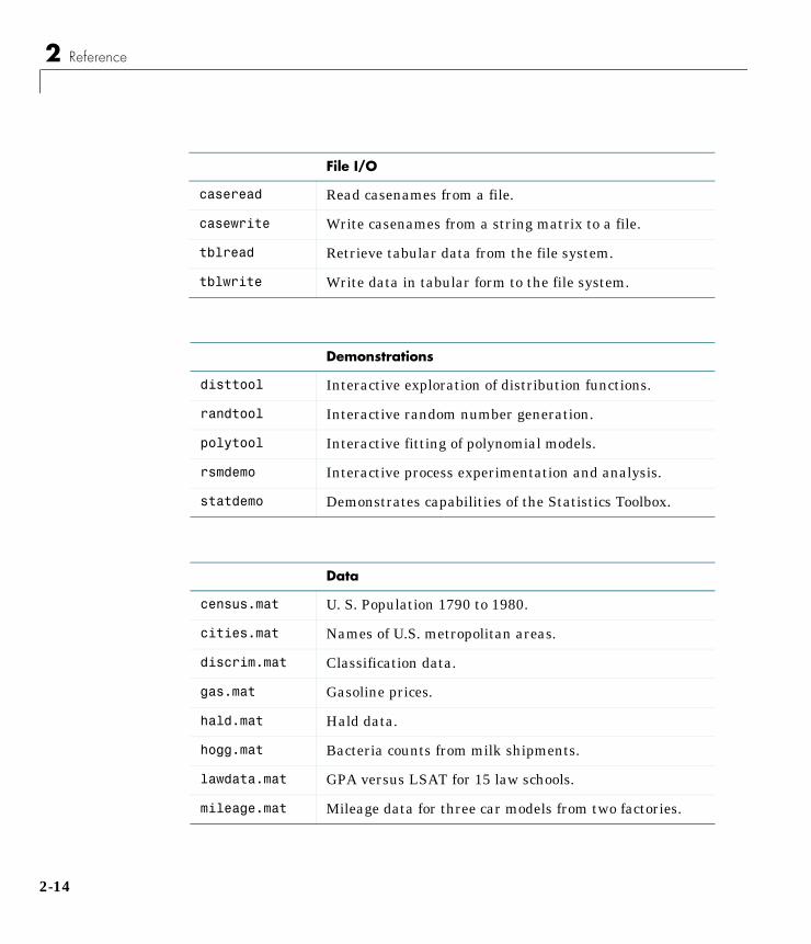
2 Reference
File I/O
caseread Read casenames from a file.
casewrite Write casenames from a string matrix to a file.
tblread Retrieve tabular data from the file system.
tblwrite Write data in tabular form to the file system.
Demonstrations
disttool Interactive exploration of distribution functions.
randtool Interactive random number generation.
polytool Interactive fitting of polynomial models.
rsmdemo Interactive process experimentation and analysis.
statdemo Demonstrates capabilities of the Statistics Toolbox.
Data
census.mat U. S. Population 1790 to 1980.
cities.mat Names of U.S. metropolitan areas.
discrim.mat Classification data.
gas.mat Gasoline prices.
hald.mat Hald data.
hogg.mat Bacteria counts from milk shipments.
lawdata.mat GPA versus LSAT for 15 law schools.
mileage.mat Mileage data for three car models from two factories.
2-14
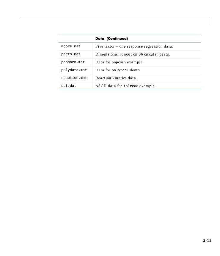
moore.mat Five factor – one response regression data.
parts.mat Dimensional runout on 36 circular parts.
popcorn.mat Data for popcorn example.
polydata.mat Data for polytool demo.
reaction.mat Reaction kinetics data.
sat.dat ASCII data for tblread example.
Data (Continued)
2-15
anova1
2-16
2anova1
2
Purpose One-way Analysis of Variance (ANOVA).
Syntax p = anova1(X)
p = anova1(x,group)
Description anova1(X) performs a balanced one-way ANOVA for comparing the means oftwo or more columns of data on the sample in X. It returns the p-value for thenull hypothesis that the means of the columns of X are equal. If the p-value isnear zero, this casts doubt on the null hypothesis and suggests that the meansof the columns are, in fact, different.
anova1(x,group) performs a one-way ANOVA for comparing the means of twoor more samples of data in x indexed by the vector, group. The input, group,identifies the group of the corresponding element of the vector x.
The values of group are integers with minimum equal to one and maximumequal to the number of different groups to compare. There must be at least oneelement in each group. This two-input form of anova1 does not require equalnumbers of elements in each group, so it is appropriate for unbalanced data.
The choice of a limit for the p-value to determine whether the result is“statistically significant” is left to the researcher. It is common to declare aresult significant if the p-value is less than 0.05 or 0.01.
anova1 also displays two figures.
The first figure is the standard ANOVA table, which divides the variability ofthe data in X into two parts:
• The variability due to the differences among the column means.
• The variability due to the differences between the data in each column andthe column mean.
The ANOVA table has five columns:
• The first shows the source of the variability.
• The second shows the Sum of Squares (SS) due to each source.
• The third shows the degrees of freedom (df) associated with each source.
• The fourth shows the Mean Squares (MS), which is the ratio SS/df.
• The fifth shows the F statistic, which is the ratio of the MS’s.
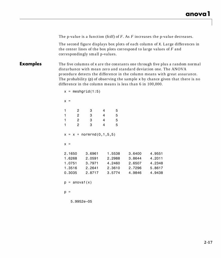
anova1
The p-value is a function (fcdf) of F. As F increases the p-value decreases.
The second figure displays box plots of each column of X. Large differences inthe center lines of the box plots correspond to large values of F andcorrespondingly small p-values.
Examples The five columns of x are the constants one through five plus a random normaldisturbance with mean zero and standard deviation one. The ANOVAprocedure detects the difference in the column means with great assurance.The probability (p) of observing the sample x by chance given that there is nodifference in the column means is less than 6 in 100,000.
x = meshgrid(1:5)
x =
1 2 3 4 51 2 3 4 51 2 3 4 51 2 3 4 5
x = x + normrnd(0,1,5,5)
x =
2.1650 3.6961 1.5538 3.6400 4.95511.6268 2.0591 2.2988 3.8644 4.20111.0751 3.7971 4.2460 2.6507 4.23481.3516 2.2641 2.3610 2.7296 5.86170.3035 2.8717 3.5774 4.9846 4.9438
p = anova1(x)
p =
5.9952e–05
2-17

anova1
The following example comes from a study of material strength in structuralbeams Hogg (1987). The vector, strength, measures the deflection of a beam inthousandths of an inch under 3,000 pounds of force. Stronger beams deflectless. The civil engineer performing the study wanted to determine whether thestrength of steel beams was equal to the strength of two more expensive alloys.Steel is coded 1 in the vector, alloy. The other materials are coded 2 and 3.
strength = [82 86 79 83 84 85 86 87 74 82 78 75 76 77 79 ...79 77 78 82 79];alloy =[1 1 1 1 1 1 1 1 2 2 2 2 2 2 3 3 3 3 3 3];
ANOVA Table
Source SS df MS F Columns 32.93 4 8.232 11.26Error 14.62 20 0.7312Total 47.55 24
1 2 3 4 5
1
2
3
4
5
6
Val
ues
Column Number
2-18

anova1
Though alloy is sorted in this example, you do not need to sort the groupingvariable.
p = anova1(strength,alloy)p =
1.5264e–04
The p-value indicates that the three alloys are significantly different. The boxplot confirms this graphically and shows that the steel beams deflect more thanthe more expensive alloys.
References Hogg, R. V., and J. Ledolter. Engineering Statistics. MacMillan PublishingCompany, 1987.
ANOVA Table
Source SS df MS F Columns 184.8 2 92.4 15.4Error 102 17 6Total 286.8 19
1 2 3
75
80
85
Val
ues
Group Number
2-19
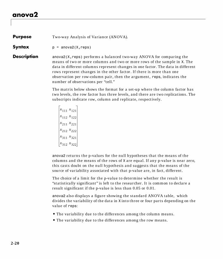
anova2
2anova2Purpose Two-way Analysis of Variance (ANOVA).
Syntax p = anova2(X,reps)
Description anova2(X,reps) performs a balanced two-way ANOVA for comparing themeans of two or more columns and two or more rows of the sample in X. Thedata in different columns represent changes in one factor. The data in differentrows represent changes in the other factor. If there is more than oneobservation per row-column pair, then the argument, reps, indicates thenumber of observations per “cell.”
The matrix below shows the format for a set-up where the column factor hastwo levels, the row factor has three levels, and there are two replications. Thesubscripts indicate row, column and replicate, respectively.
anova2 returns the p-values for the null hypotheses that the means of thecolumns and the means of the rows of X are equal. If any p-value is near zero,this casts doubt on the null hypothesis and suggests that the means of thesource of variability associated with that p-value are, in fact, different.
The choice of a limit for the p-value to determine whether the result is“statistically significant” is left to the researcher. It is common to declare aresult significant if the p-value is less than 0.05 or 0.01.
anova2 also displays a figure showing the standard ANOVA table, whichdivides the variability of the data in X into three or four parts depending on thevalue of reps:
• The variability due to the differences among the column means.
• The variability due to the differences among the row means.
x111 x121
x112 x122
x211 x221
x212 x222
x311 x321
x312 x322
2-20

anova2
• The variability due to the interaction between rows and columns (if reps isgreater than its default value of one.)
• The remaining variability not explained by any systematic source.
The ANOVA table has five columns:
• The first shows the source of the variability.
• The second shows the Sum of Squares (SS) due to each source.
• The third shows the degrees of freedom (df) associated with each source.
• The fourth shows the Mean Squares (MS), which is the ratio SS/df.
• The fifth shows the F statistics, which is the ratio of the mean squares.
The p-value is a function (fcdf) of F. As F increases the p-value decreases.
Examples The data below comes from a study of popcorn brands and popper type (Hogg1987). The columns of the matrix popcorn are brands (Gourmet, National, andGeneric). The rows are popper type (Oil and Air.) The study popped a batch of
2-21
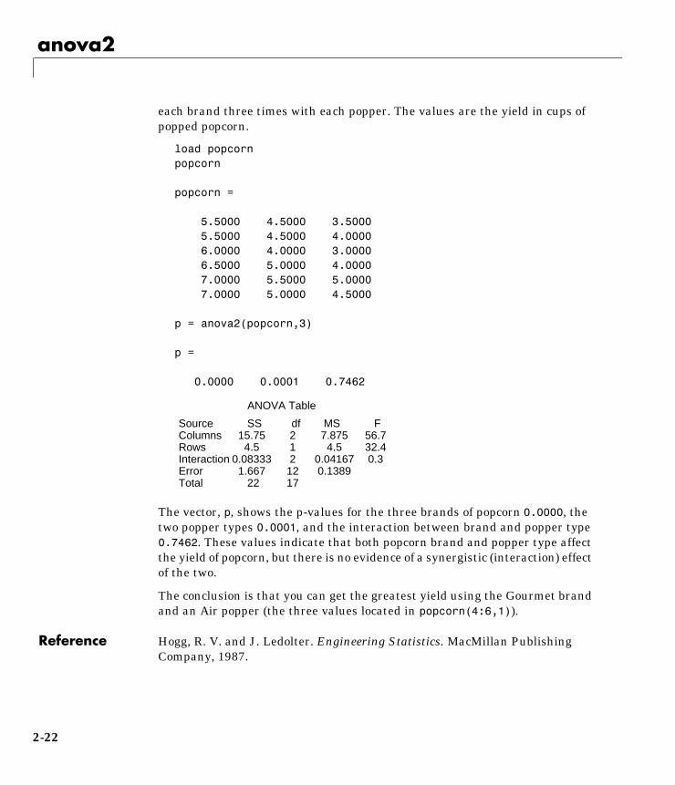
anova2
each brand three times with each popper. The values are the yield in cups ofpopped popcorn.
load popcornpopcorn
popcorn =
5.5000 4.5000 3.5000 5.5000 4.5000 4.0000 6.0000 4.0000 3.0000 6.5000 5.0000 4.0000 7.0000 5.5000 5.0000 7.0000 5.0000 4.5000
p = anova2(popcorn,3)
p =
0.0000 0.0001 0.7462
The vector, p, shows the p-values for the three brands of popcorn 0.0000, thetwo popper types 0.0001, and the interaction between brand and popper type0.7462. These values indicate that both popcorn brand and popper type affectthe yield of popcorn, but there is no evidence of a synergistic (interaction) effectof the two.
The conclusion is that you can get the greatest yield using the Gourmet brandand an Air popper (the three values located in popcorn(4:6,1)).
Reference Hogg, R. V. and J. Ledolter. Engineering Statistics. MacMillan PublishingCompany, 1987.
ANOVA Table
Source SS df MS F Columns 15.75 2 7.875 56.7Rows 4.5 1 4.5 32.4Interaction 0.08333 2 0.04167 0.3Error 1.667 12 0.1389Total 22 17
2-22
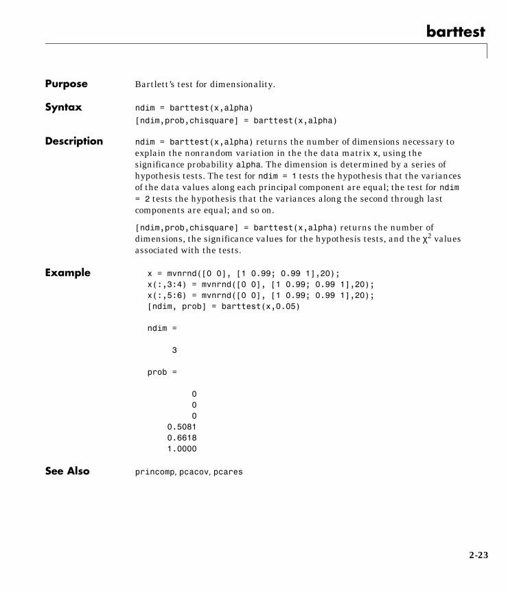
barttest
2barttestPurpose Bartlett’s test for dimensionality.
Syntax ndim = barttest(x,alpha)
[ndim,prob,chisquare] = barttest(x,alpha)
Description ndim = barttest(x,alpha) returns the number of dimensions necessary toexplain the nonrandom variation in the the data matrix x, using thesignificance probability alpha. The dimension is determined by a series ofhypothesis tests. The test for ndim = 1 tests the hypothesis that the variancesof the data values along each principal component are equal; the test for ndim = 2 tests the hypothesis that the variances along the second through lastcomponents are equal; and so on.
[ndim,prob,chisquare] = barttest(x,alpha) returns the number ofdimensions, the significance values for the hypothesis tests, and the χ2 valuesassociated with the tests.
Example x = mvnrnd([0 0], [1 0.99; 0.99 1],20);x(:,3:4) = mvnrnd([0 0], [1 0.99; 0.99 1],20);x(:,5:6) = mvnrnd([0 0], [1 0.99; 0.99 1],20);[ndim, prob] = barttest(x,0.05)
ndim =
3
prob =
0 0 0 0.5081 0.6618 1.0000
See Also princomp, pcacov, pcares
2-23
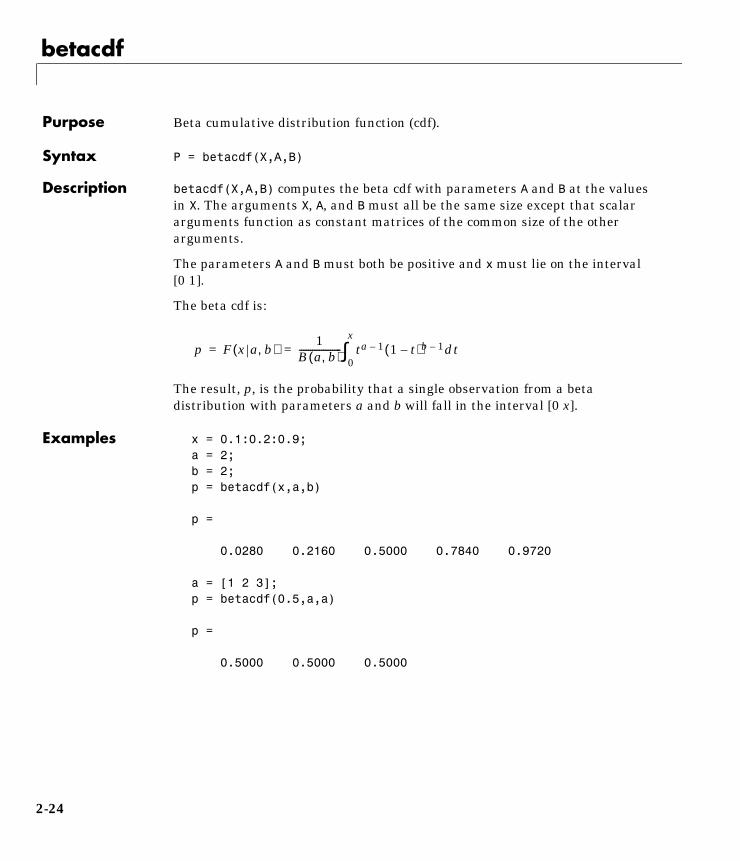
betacdf
2betacdfPurpose Beta cumulative distribution function (cdf).
Syntax P = betacdf(X,A,B)
Description betacdf(X,A,B) computes the beta cdf with parameters A and B at the valuesin X. The arguments X, A, and B must all be the same size except that scalararguments function as constant matrices of the common size of the otherarguments.
The parameters A and B must both be positive and x must lie on the interval[0 1].
The beta cdf is:
The result, p, is the probability that a single observation from a betadistribution with parameters a and b will fall in the interval [0 x].
Examples x = 0.1:0.2:0.9;a = 2;b = 2;p = betacdf(x,a,b)
p =
0.0280 0.2160 0.5000 0.7840 0.9720
a = [1 2 3];p = betacdf(0.5,a,a)
p =
0.5000 0.5000 0.5000
p F x a b,( )1
B a b,( )------------------- ta 1–
0
x
∫ 1 t–( )b 1– dt= =
2-24
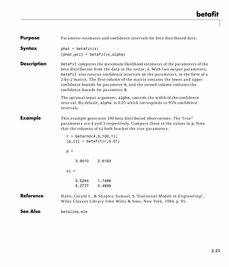
betafit
2betafitPurpose Parameter estimates and confidence intervals for beta distributed data.
Syntax phat = betafit(x)
[phat,pci] = betafit(x,alpha)
Description betafit computes the maximum likelihood estimates of the parameters of thebeta distribution from the data in the vector, x. With two output parameters,betafit also returns confidence intervals on the parameters, in the form of a2-by-2 matrix. The first column of the matrix contains the lower and upperconfidence bounds for parameter A, and the second column contains theconfidence bounds for parameter B.
The optional input argument, alpha, controls the width of the confidenceinterval. By default, alpha is 0.05 which corresponds to 95% confidenceintervals.
Example This example generates 100 beta distributed observations. The “true”parameters are 4 and 3 respectively. Compare these to the values in p. Notethat the columns of ci both bracket the true parameters.
r = betarnd(4,3,100,1);[p,ci] = betafit(r,0.01)
p =
3.9010 2.6193
ci =
2.5244 1.7488 5.2777 3.4899
Reference Hahn, Gerald J., & Shapiro, Samuel, S."Statistical Models in Engineering",Wiley Classics Library John Wiley & Sons, New York. 1994. p. 95.
See Also betalike, mle
2-25
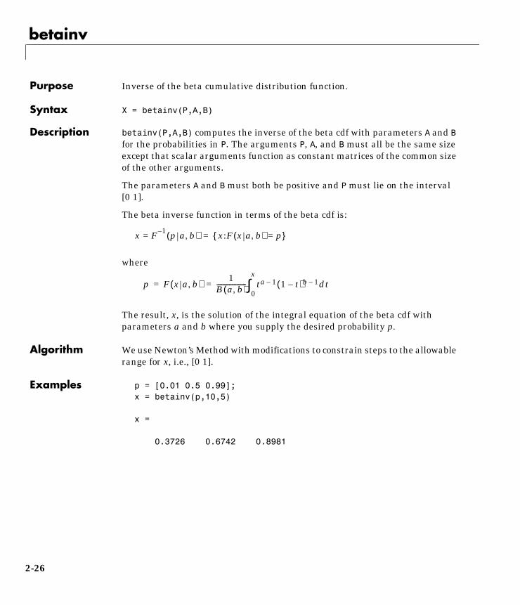
betainv
2betainvPurpose Inverse of the beta cumulative distribution function.
Syntax X = betainv(P,A,B)
Description betainv(P,A,B) computes the inverse of the beta cdf with parameters A and Bfor the probabilities in P. The arguments P, A, and B must all be the same sizeexcept that scalar arguments function as constant matrices of the common sizeof the other arguments.
The parameters A and B must both be positive and P must lie on the interval[0 1].
The beta inverse function in terms of the beta cdf is:
where
The result, x, is the solution of the integral equation of the beta cdf withparameters a and b where you supply the desired probability p.
Algorithm We use Newton’s Method with modifications to constrain steps to the allowablerange for x, i.e., [0 1].
Examples p = [0.01 0.5 0.99];x = betainv(p,10,5)
x =
0.3726 0.6742 0.8981
x F 1–= p a b,( ) x:F x a b,( ) p={ }=
p F x a b,( )1
B a b,( )------------------- ta 1–
0
x
∫ 1 t–( )b 1– dt= =
2-26
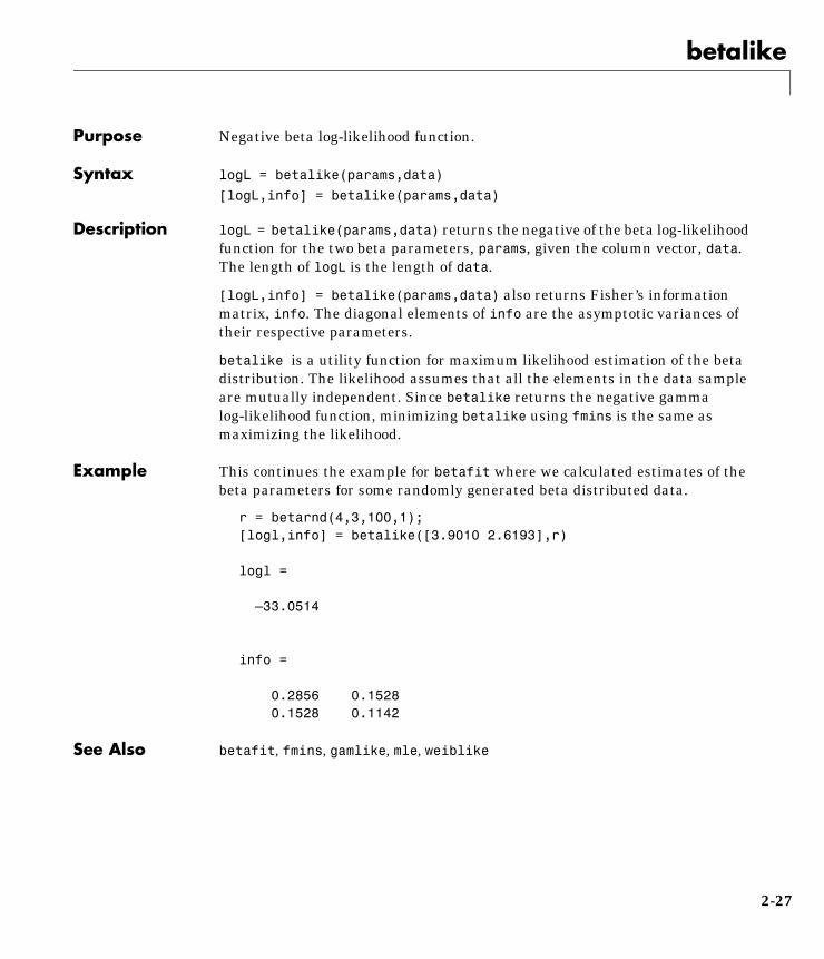
betalike
2betalikePurpose Negative beta log-likelihood function.
Syntax logL = betalike(params,data)
[logL,info] = betalike(params,data)
Description logL = betalike(params,data) returns the negative of the beta log-likelihoodfunction for the two beta parameters, params, given the column vector, data.The length of logL is the length of data.
[logL,info] = betalike(params,data) also returns Fisher’s informationmatrix, info. The diagonal elements of info are the asymptotic variances oftheir respective parameters.
betalike is a utility function for maximum likelihood estimation of the betadistribution. The likelihood assumes that all the elements in the data sampleare mutually independent. Since betalike returns the negative gammalog-likelihood function, minimizing betalike using fmins is the same asmaximizing the likelihood.
Example This continues the example for betafit where we calculated estimates of thebeta parameters for some randomly generated beta distributed data.
r = betarnd(4,3,100,1);[logl,info] = betalike([3.9010 2.6193],r)
logl =
–33.0514
info =
0.2856 0.1528 0.1528 0.1142
See Also betafit, fmins, gamlike, mle, weiblike
2-27
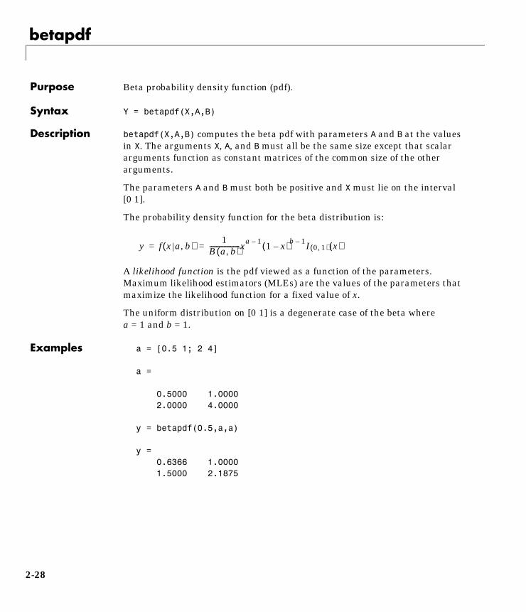
betapdf
2betapdfPurpose Beta probability density function (pdf).
Syntax Y = betapdf(X,A,B)
Description betapdf(X,A,B) computes the beta pdf with parameters A and B at the valuesin X. The arguments X, A, and B must all be the same size except that scalararguments function as constant matrices of the common size of the otherarguments.
The parameters A and B must both be positive and X must lie on the interval[0 1].
The probability density function for the beta distribution is:
A likelihood function is the pdf viewed as a function of the parameters.Maximum likelihood estimators (MLEs) are the values of the parameters thatmaximize the likelihood function for a fixed value of x.
The uniform distribution on [0 1] is a degenerate case of the beta wherea = 1 and b = 1.
Examples a = [0.5 1; 2 4]
a =
0.5000 1.0000 2.0000 4.0000
y = betapdf(0.5,a,a)
y = 0.6366 1.0000 1.5000 2.1875
y f x a b,( )1
B a b,( )-------------------xa 1– 1 x–( )b 1– I 0 1,( ) x( )= =
2-28

betarnd
2betarndPurpose Random numbers from the beta distribution.
Syntax R = betarnd(A,B)R = betarnd(A,B,m)R = betarnd(A,B,m,n)
Description R = betarnd(A,B) generates beta random numbers with parameters A and B.The size of R is the common size of A and B if both are matrices. If eitherparameter is a scalar, the size of R is the size of the other.
R = betarnd(A,B,m) generates beta random numbers with parameters A andB. m is a 1-by-2 vector that contains the row and column dimensions of r.
R = betarnd(A,B,m,n) generates an m by n matrix of beta random numberswith parameters A and B.
Examples a = [1 1; 2 2];b = [1 2; 1 2];r = betarnd(a,b)
r =
0.6987 0.6139 0.9102 0.8067
r = betarnd(10,10,[1 5])
r =
0.5974 0.4777 0.5538 0.5465 0.6327
r = betarnd(4,2,2,3)
r =
0.3943 0.6101 0.5768 0.5990 0.2760 0.5474
2-29

betastat
2betastatPurpose Mean and variance for the beta distribution.
Syntax [M,V] = betastat(A,B)
Description For the beta distribution:
• The mean is
• The variance is
Examples If the parameters are equal, the mean is 1/2.
a = 1:6;[m,v] = betastat(a,a)
m =
0.5000 0.5000 0.5000 0.5000 0.5000 0.5000
v =
0.0833 0.0500 0.0357 0.0278 0.0227 0.0192
aa b+-------------
aba b 1+ +( ) a b+( )2-------------------------------------------------
2-30

binocdf
2binocdfPurpose Binomial cumulative distribution function (cdf).
Syntax Y = binocdf(X,N,P)
Description binocdf(X,N,P) computes the binomial cdf with parameters N and P at thevalues in X. The arguments X, N, and P must all be the same size except thatscalar arguments function as constant matrices of the common size of the otherarguments.
The parameter N must be a positive integer and P must lie on the interval [0 1].
The binomial cdf is:
The result, y, is the probability of observing up to x successes in n independenttrials of where the probability of success in any given trial is p.
Examples If a baseball team plays 162 games in a season and has a 50-50 chance ofwinning any game, then the probability of that team winning more than 100games in a season is:
1 – binocdf(100,162,0.5)
The result is 0.001 (i.e., 1 – 0.999). If a team wins 100 or more games in aseason, this result suggests that it is likely that the team’s true probability ofwinning any game is greater than 0.5.
y F x n p,( )ni
i 0=
x
∑ piq 1 i–( )I 0 1 … n, , ,( ) i( )= =
2-31
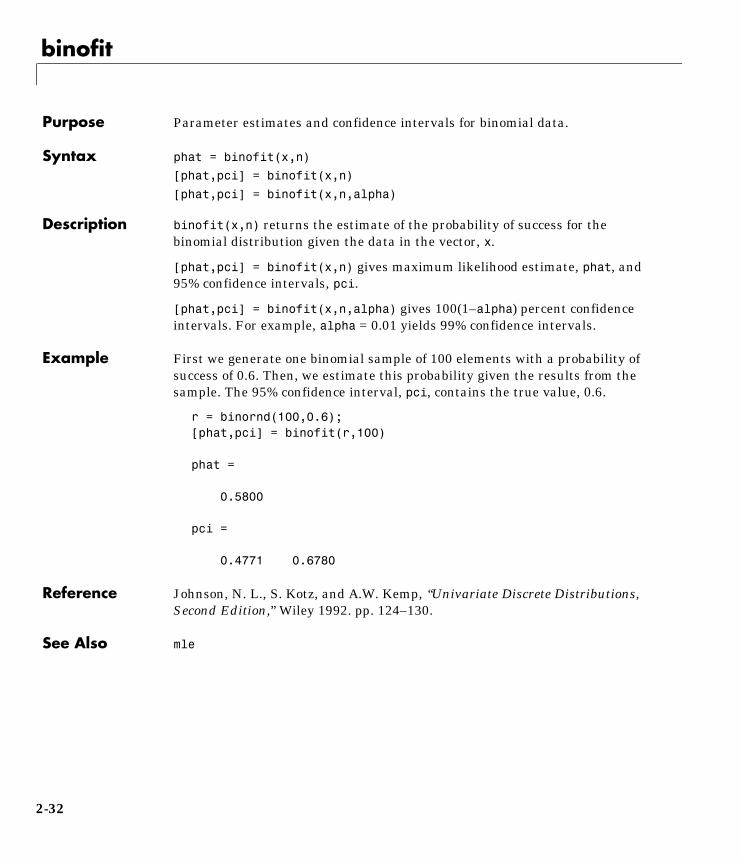
binofit
2binofitPurpose Parameter estimates and confidence intervals for binomial data.
Syntax phat = binofit(x,n)
[phat,pci] = binofit(x,n)
[phat,pci] = binofit(x,n,alpha)
Description binofit(x,n) returns the estimate of the probability of success for thebinomial distribution given the data in the vector, x.
[phat,pci] = binofit(x,n) gives maximum likelihood estimate, phat, and95% confidence intervals, pci.
[phat,pci] = binofit(x,n,alpha) gives 100(1–alpha) percent confidenceintervals. For example, alpha = 0.01 yields 99% confidence intervals.
Example First we generate one binomial sample of 100 elements with a probability ofsuccess of 0.6. Then, we estimate this probability given the results from thesample. The 95% confidence interval, pci, contains the true value, 0.6.
r = binornd(100,0.6);[phat,pci] = binofit(r,100)
phat =
0.5800
pci =
0.4771 0.6780
Reference Johnson, N. L., S. Kotz, and A.W. Kemp, “Univariate Discrete Distributions,Second Edition,” Wiley 1992. pp. 124–130.
See Also mle
2-32
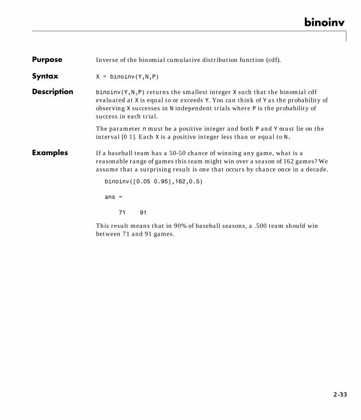
binoinv
2binoinvPurpose Inverse of the binomial cumulative distribution function (cdf).
Syntax X = binoinv(Y,N,P)
Description binoinv(Y,N,P) returns the smallest integer X such that the binomial cdfevaluated at X is equal to or exceeds Y. You can think of Y as the probability ofobserving X successes in N independent trials where P is the probability ofsuccess in each trial.
The parameter n must be a positive integer and both P and Y must lie on theinterval [0 1]. Each X is a positive integer less than or equal to N.
Examples If a baseball team has a 50-50 chance of winning any game, what is areasonable range of games this team might win over a season of 162 games? Weassume that a surprising result is one that occurs by chance once in a decade.
binoinv([0.05 0.95],162,0.5)
ans =
71 91
This result means that in 90% of baseball seasons, a .500 team should winbetween 71 and 91 games.
2-33
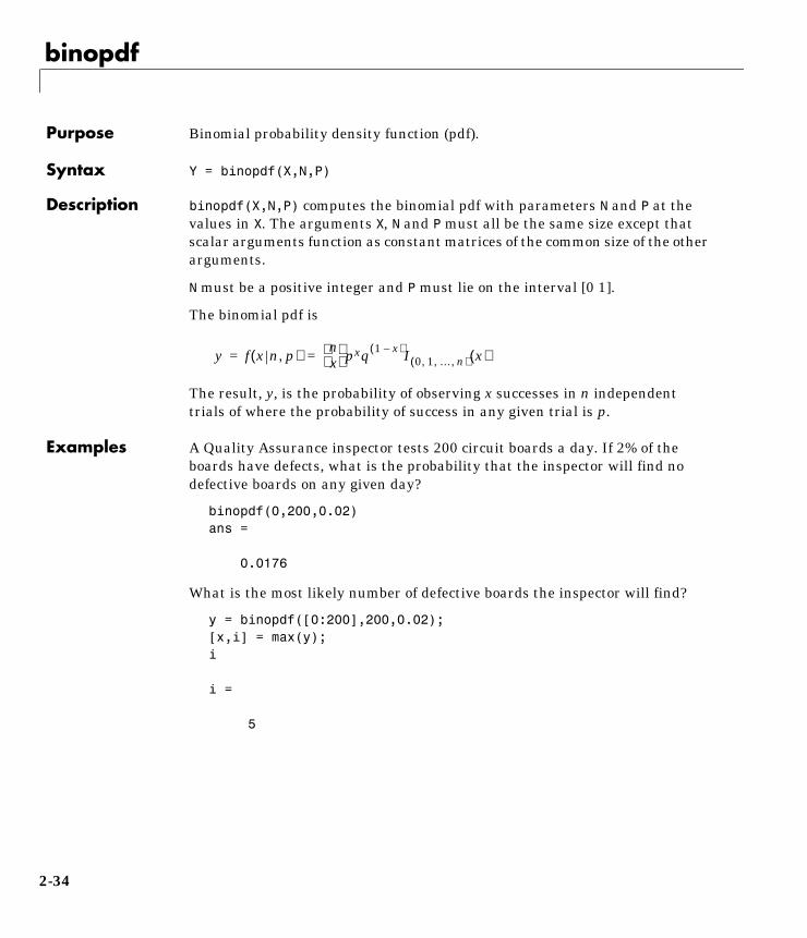
binopdf
2binopdfPurpose Binomial probability density function (pdf).
Syntax Y = binopdf(X,N,P)
Description binopdf(X,N,P) computes the binomial pdf with parameters N and P at thevalues in X. The arguments X, N and P must all be the same size except thatscalar arguments function as constant matrices of the common size of the otherarguments.
N must be a positive integer and P must lie on the interval [0 1].
The binomial pdf is
The result, y, is the probability of observing x successes in n independenttrials of where the probability of success in any given trial is p.
Examples A Quality Assurance inspector tests 200 circuit boards a day. If 2% of theboards have defects, what is the probability that the inspector will find nodefective boards on any given day?
binopdf(0,200,0.02)ans =
0.0176
What is the most likely number of defective boards the inspector will find?
y = binopdf([0:200],200,0.02);[x,i] = max(y);i
i =
5
y f x n p,( ) nx
pxq 1 x–( )I 0 1 … n, , ,( ) x( )= =
2-34
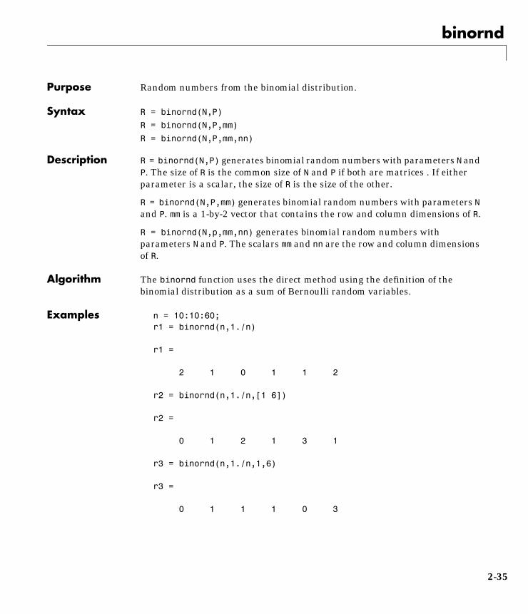
binornd
2binorndPurpose Random numbers from the binomial distribution.
Syntax R = binornd(N,P)
R = binornd(N,P,mm)
R = binornd(N,P,mm,nn)
Description R = binornd(N,P) generates binomial random numbers with parameters N andP. The size of R is the common size of N and P if both are matrices . If eitherparameter is a scalar, the size of R is the size of the other.
R = binornd(N,P,mm) generates binomial random numbers with parameters Nand P. mm is a 1-by-2 vector that contains the row and column dimensions of R.
R = binornd(N,p,mm,nn) generates binomial random numbers withparameters N and P. The scalars mm and nn are the row and column dimensionsof R.
Algorithm The binornd function uses the direct method using the definition of thebinomial distribution as a sum of Bernoulli random variables.
Examples n = 10:10:60;r1 = binornd(n,1./n)
r1 =
2 1 0 1 1 2
r2 = binornd(n,1./n,[1 6])
r2 =
0 1 2 1 3 1
r3 = binornd(n,1./n,1,6)
r3 =
0 1 1 1 0 3
2-35
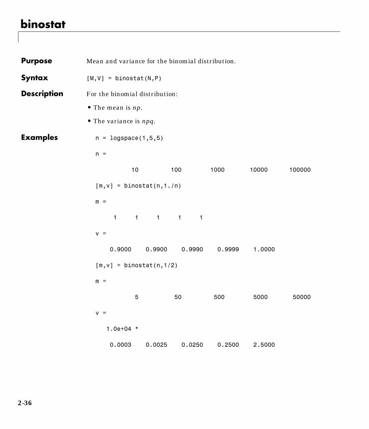
binostat
2binostatPurpose Mean and variance for the binomial distribution.
Syntax [M,V] = binostat(N,P)
Description For the binomial distribution:
• The mean is np.
• The variance is npq.
Examples n = logspace(1,5,5)
n =
10 100 1000 10000 100000
[m,v] = binostat(n,1./n)
m =
1 1 1 1 1
v =
0.9000 0.9900 0.9990 0.9999 1.0000
[m,v] = binostat(n,1/2)
m =
5 50 500 5000 50000
v =
1.0e+04 *
0.0003 0.0025 0.0250 0.2500 2.5000
2-36
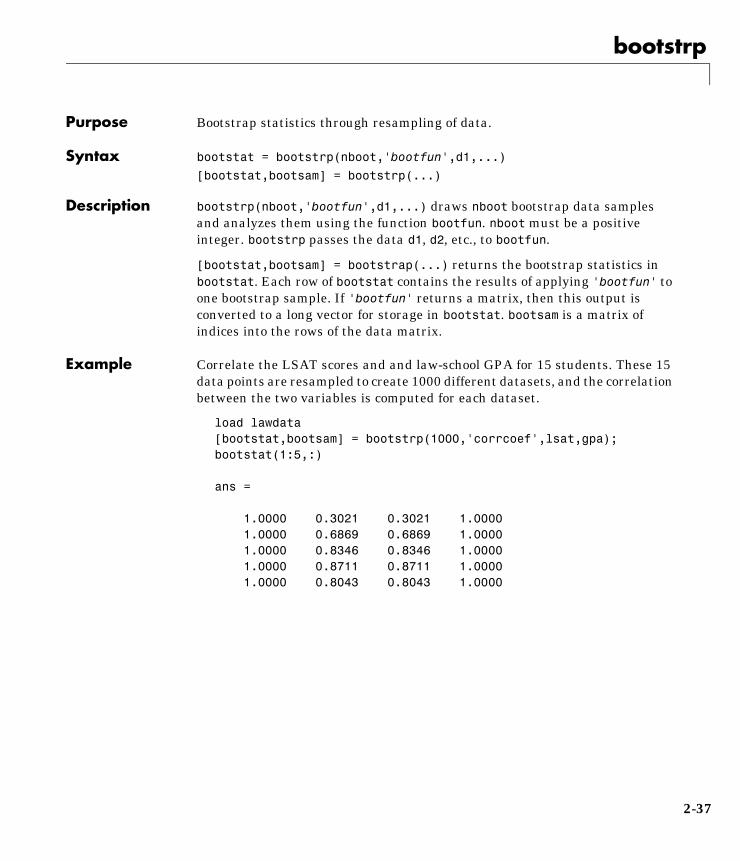
bootstrp
2bootstrpPurpose Bootstrap statistics through resampling of data.
Syntax bootstat = bootstrp(nboot,'bootfun',d1,...)
[bootstat,bootsam] = bootstrp(...)
Description bootstrp(nboot,'bootfun',d1,...) draws nboot bootstrap data samplesand analyzes them using the function bootfun. nboot must be a positiveinteger. bootstrp passes the data d1, d2, etc., to bootfun.
[bootstat,bootsam] = bootstrap(...) returns the bootstrap statistics inbootstat. Each row of bootstat contains the results of applying 'bootfun' toone bootstrap sample. If 'bootfun' returns a matrix, then this output isconverted to a long vector for storage in bootstat. bootsam is a matrix ofindices into the rows of the data matrix.
Example Correlate the LSAT scores and and law-school GPA for 15 students. These 15data points are resampled to create 1000 different datasets, and the correlationbetween the two variables is computed for each dataset.
load lawdata[bootstat,bootsam] = bootstrp(1000,'corrcoef',lsat,gpa);bootstat(1:5,:)
ans =
1.0000 0.3021 0.3021 1.0000 1.0000 0.6869 0.6869 1.0000 1.0000 0.8346 0.8346 1.0000 1.0000 0.8711 0.8711 1.0000 1.0000 0.8043 0.8043 1.0000
2-37
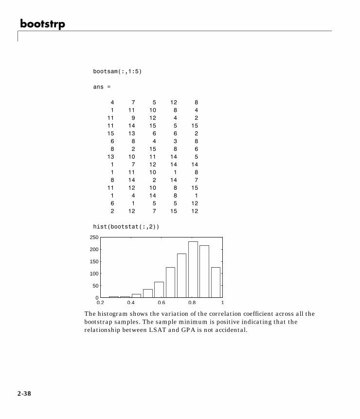
bootstrp
bootsam(:,1:5)
ans =
4 7 5 12 8 1 11 10 8 4 11 9 12 4 2 11 14 15 5 15 15 13 6 6 2 6 8 4 3 8 8 2 15 8 6 13 10 11 14 5 1 7 12 14 14 1 11 10 1 8 8 14 2 14 7 11 12 10 8 15 1 4 14 8 1 6 1 5 5 12 2 12 7 15 12
hist(bootstat(:,2))
The histogram shows the variation of the correlation coefficient across all thebootstrap samples. The sample minimum is positive indicating that therelationship between LSAT and GPA is not accidental.
0.2 0.4 0.6 0.8 10
50
100
150
200
250
2-38

boxplot
2boxplotPurpose Box plots of a data sample.
Syntax boxplot(X)
boxplot(X,notch)
boxplot(X,notch,'sym')
boxplot(X,notch,'sym',vert)
boxplot(X,notch,'sym',vert,whis)
Description boxplot(X) produces a box and whisker plot for each column of X. The box haslines at the lower quartile, median, and upper quartile values. The whiskersare lines extending from each end of the box to show the extent of the rest ofthe data. Outliers are data with values beyond the ends of the whiskers. Ifthere is no data outside the whisker, there is a dot at the bottom whisker. Thedot color is the same as the whisker color.
boxplot(X,notch) with notch = 1 produces a notched-box plot. Notches grapha robust estimate of the uncertainty about the means for box to boxcomparison. The default, notch = 0 produces a rectangular box plot.
boxplot(X,notch,'sym') where 'sym' is a plotting symbol allows control ofthe symbol for outliers if any (default = '+').
boxplot(X,notch,'sym',vert) with vert = 0 makes the boxes horizontal(default: vert = 1, for vertical)
boxplot(X,notch,'sym',vert,whis) enables you to specify the length of the“whiskers”. whis defines the length of the whiskers as a function of theinter-quartile range (default = 1.5 * IQR.) If whis = 0, then boxplot displays alldata values outside the box using the plotting symbol, 'sym'.
2-39

boxplot
Examples x1 = normrnd(5,1,100,1);x2 = normrnd(6,1,100,1);x = [x1 x2];boxplot(x,1)
The difference between the means of the two columns of x is 1. We can detectthis difference graphically since the notches do not overlap.
1 2
3
4
5
6
7
8
Val
ues
Column Number
2-40
capable
2capablePurpose Process capability indices.
Syntax p = capable(data,lower,upper)
[p,Cp,Cpk] = capable(data,lower,upper)
Description capable(data,lower,upper) computes the probability that a sample, data,from some process falls outside the bounds specified in lower and upper.
The assumptions are that the measured values in the vector, data, arenormally distributed with constant mean and variance and the themeasurements are statistically independent.
[p,Cp,Cpk] = capable(data,lower,upper) also returns the capability indicesCp and Cpk.
Cp is the ratio of the range of the specifications to six times the estimate of theprocess standard deviation
For a process that has its average value on target, a Cp of one translates to alittle more than one defect per thousand. Recently many industries have set aquality goal of one part per million. This would correspond to a Cp = 1.6. Thehigher the value of Cp the more capable the process.
Cpk is the ratio of difference between the process mean and the closerspecification limit to three times the estimate of the process standard deviation
where the process mean is µ. For processes that do not maintain their averageon target, Cpk is a more descriptive index of process capability.
Example Imagine a machined part with specifications requiring a dimension to bewithin three thousandths of an inch of nominal. Suppose that the machiningprocess cuts too thick by one thousandth of an inch on average and also has a
CpUSL LSL–
6σ--------------------------------=
Cpk minUSL µ–
3σ-----------------------µ LSL–
3σ----------------------, =
2-41

capable
standard deviation of one thousandth of an inch. What are the capabilityindices of this process?
data = normrnd(1,1,30,1);[p,Cp,Cpk] = capable(data,[–3 3]);indices = [p Cp Cpk]
indices =
0.0172 1.1144 0.7053
We expect 17 parts out of a thousand to be out-of-specification. Cpk is less thanCp because the process is not centered.
Reference Montgomery, D., “Introduction to Statistical Quality Control,” John Wiley &Sons 1991. pp. 369–374.
See Also capaplot, histfit
2-42
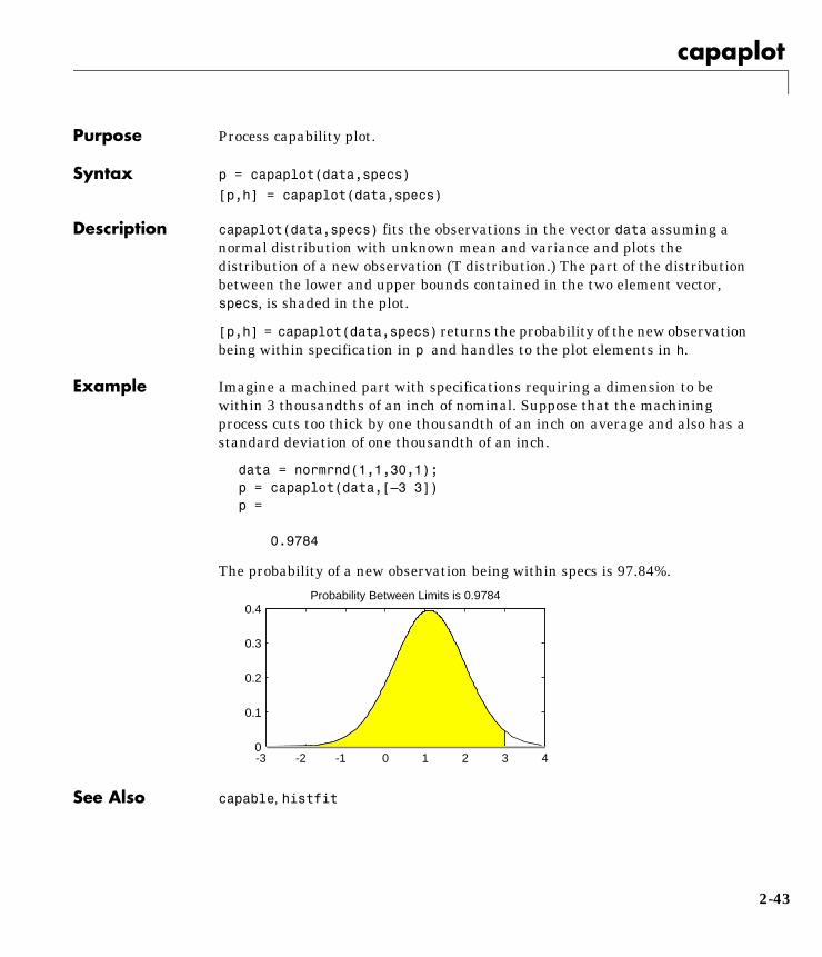
capaplot
2capaplotPurpose Process capability plot.
Syntax p = capaplot(data,specs)
[p,h] = capaplot(data,specs)
Description capaplot(data,specs) fits the observations in the vector data assuming anormal distribution with unknown mean and variance and plots thedistribution of a new observation (T distribution.) The part of the distributionbetween the lower and upper bounds contained in the two element vector,specs, is shaded in the plot.
[p,h] = capaplot(data,specs) returns the probability of the new observationbeing within specification in p and handles to the plot elements in h.
Example Imagine a machined part with specifications requiring a dimension to bewithin 3 thousandths of an inch of nominal. Suppose that the machiningprocess cuts too thick by one thousandth of an inch on average and also has astandard deviation of one thousandth of an inch.
data = normrnd(1,1,30,1);p = capaplot(data,[–3 3])p =
0.9784
The probability of a new observation being within specs is 97.84%.
See Also capable, histfit
-3 -2 -1 0 1 2 3 40
0.1
0.2
0.3
0.4Probability Between Limits is 0.9784
2-43
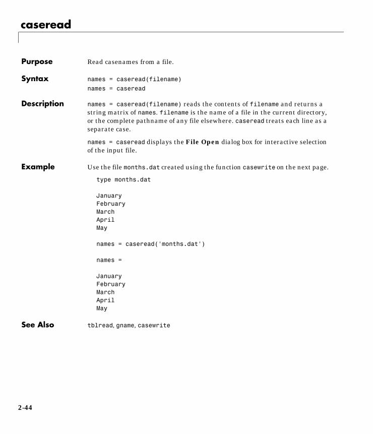
caseread
2casereadPurpose Read casenames from a file.
Syntax names = caseread(filename)
names = caseread
Description names = caseread(filename) reads the contents of filename and returns astring matrix of names. filename is the name of a file in the current directory,or the complete pathname of any file elsewhere. caseread treats each line as aseparate case.
names = caseread displays the File Open dialog box for interactive selectionof the input file.
Example Use the file months.dat created using the function casewrite on the next page.
type months.dat
JanuaryFebruaryMarchAprilMay
names = caseread('months.dat')
names =
January FebruaryMarch April May
See Also tblread, gname, casewrite
2-44
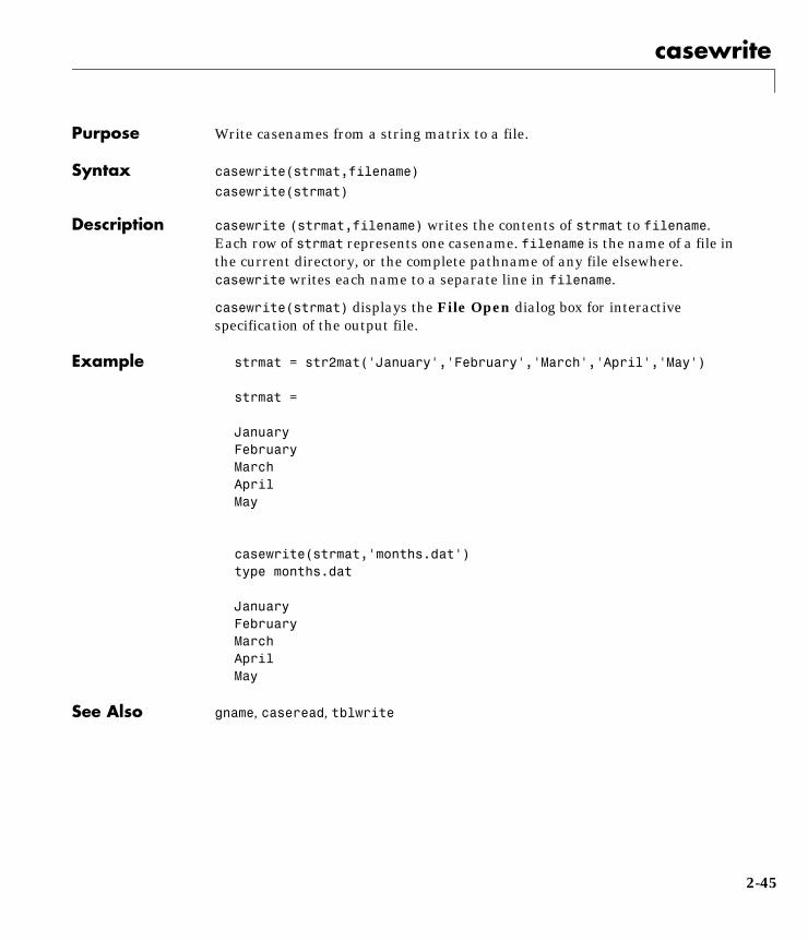
casewrite
2casewritePurpose Write casenames from a string matrix to a file.
Syntax casewrite(strmat,filename)
casewrite(strmat)
Description casewrite (strmat,filename) writes the contents of strmat to filename.Each row of strmat represents one casename. filename is the name of a file inthe current directory, or the complete pathname of any file elsewhere.casewrite writes each name to a separate line in filename.
casewrite(strmat) displays the File Open dialog box for interactivespecification of the output file.
Example strmat = str2mat('January','February','March','April','May')
strmat =
January FebruaryMarch April May
casewrite(strmat,'months.dat')type months.dat
January FebruaryMarch April May
See Also gname, caseread, tblwrite
2-45
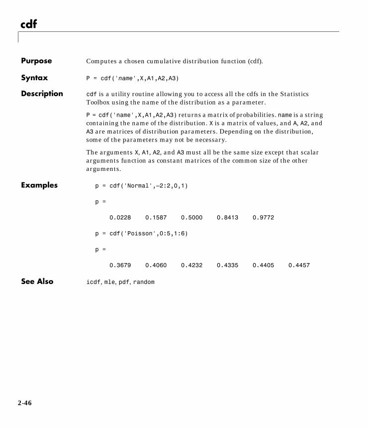
cdf
2cdfPurpose Computes a chosen cumulative distribution function (cdf).
Syntax P = cdf('name',X,A1,A2,A3)
Description cdf is a utility routine allowing you to access all the cdfs in the StatisticsToolbox using the name of the distribution as a parameter.
P = cdf('name',X,A1,A2,A3) returns a matrix of probabilities. name is a stringcontaining the name of the distribution. X is a matrix of values, and A, A2, andA3 are matrices of distribution parameters. Depending on the distribution,some of the parameters may not be necessary.
The arguments X, A1, A2, and A3 must all be the same size except that scalararguments function as constant matrices of the common size of the otherarguments.
Examples p = cdf('Normal',–2:2,0,1)
p =
0.0228 0.1587 0.5000 0.8413 0.9772
p = cdf('Poisson',0:5,1:6)
p =
0.3679 0.4060 0.4232 0.4335 0.4405 0.4457
See Also icdf, mle, pdf, random
2-46
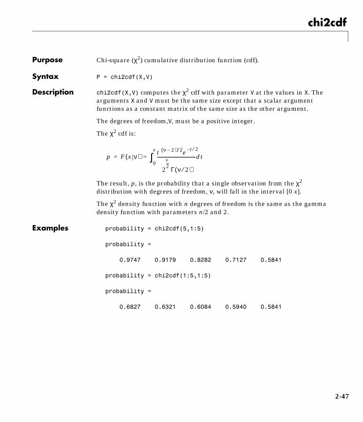
chi2cdf
2chi2cdfPurpose Chi-square (χ2) cumulative distribution function (cdf).
Syntax P = chi2cdf(X,V)
Description chi2cdf(X,V) computes the χ2 cdf with parameter V at the values in X. Thearguments X and V must be the same size except that a scalar argumentfunctions as a constant matrix of the same size as the other argument.
The degrees of freedom,V, must be a positive integer.
The χ2 cdf is:
The result, p, is the probability that a single observation from the χ2
distribution with degrees of freedom, ν, will fall in the interval [0 x].
The χ2 density function with n degrees of freedom is the same as the gammadensity function with parameters n/2 and 2.
Examples probability = chi2cdf(5,1:5)
probability =
0.9747 0.9179 0.8282 0.7127 0.5841
probability = chi2cdf(1:5,1:5)
probability =
0.6827 0.6321 0.6084 0.5940 0.5841
p F x ν( ) t ν 2–( ) 2⁄ e t– 2⁄
2
v2--- Γ ν 2⁄( )
-----------------------------------0
x
∫ dt= =
2-47
chi2inv
2chi2invPurpose Inverse of the chi-square (χ2) cumulative distribution function (cdf).
Syntax X = chi2inv(P,V)
Description chi2inv(P,V) computes the inverse of the χ2 cdf with parameter V for theprobabilities in P. The arguments P and V must be the same size except that ascalar argument functions as a constant matrix of the size of the otherargument.
The degrees of freedom,V, must be a positive integer and P must lie in theinterval [0 1].
We define the χ2 inverse function in terms of the χ2 cdf.
The result, x, is the solution of the integral equation of the χ2 cdf withparameter ν where you supply the desired probability p.
Examples Find a value that exceeds 95% of the samples from a χ2 distribution with 10degrees of freedom.
x = chi2inv(0.95,10)
x =
18.3070
You would observe values greater than 18.3 only 5% of the time by chance.
x F 1– p ν( ) x:F x ν( ) p={ }= =
where p F x ν( ) t ν 2–( ) 2⁄ e t– 2⁄
2
v2--- Γ ν 2⁄( )
-----------------------------------0
x
∫ dt= =
2-48

chi2pdf
2chi2pdfPurpose Chi-square (χ2) probability density function (pdf).
Syntax Y = chi2pdf(X,V)
Description chi2pdf(X,V) computes the χ2 pdf with parameter V at the values in X. Thearguments X and V must be the same size except that a scalar argumentfunctions as a constant matrix of the same size of the other argument.
The degrees of freedom, V, must be a positive integer.
The chi-square pdf is:
The χ2 density function with n degrees of freedom is the same as the gammadensity function with parameters n/2 and 2.
If x is standard normal , then x2 is distributed χ2 with one degree of freedom.If x1, x2, ..., xn are n independent standard normal observations, then the sumof the squares of the x’s is distributed χ2 with n degrees of freedom.
Examples nu = 1:6;x = nu;y = chi2pdf(x,nu)
y =
0.2420 0.1839 0.1542 0.1353 0.1220 0.1120
The mean of the χ2 distribution is the value of the parameter, nu. The aboveexample shows that the probability density of the mean falls as nu increases.
y f x ν( ) x ν 2–( ) 2⁄ e x– 2⁄
2
v2--- Γ ν 2⁄( )
-------------------------------------= =
2-49
chi2rnd
2chi2rndPurpose Random numbers from the chi-square (χ2) distribution.
Syntax R = chi2rnd(V)
R = chi2rnd(V,m)
R = chi2rnd(V,m,n)
Description R = chi2rnd(V) generates χ2 random numbers with V degrees of freedom. Thesize of R is the size of V.
R = chi2rnd(V,m) generates χ2 random numbers with V degrees of freedom. mis a 1-by-2 vector that contains the row and column dimensions of R.
R = chi2rnd(V,m,n) generates χ2 random numbers with V degrees of freedom.The scalars m and n are the row and column dimensions of R.
Examples Note that the first and third commands are the same but are different from thesecond command.
r = chi2rnd(1:6)
r =
0.0037 3.0377 7.8142 0.9021 3.2019 9.0729
r = chi2rnd(6,[1 6])
r =
6.5249 2.6226 12.2497 3.0388 6.3133 5.0388
r = chi2rnd(1:6,1,6)
r =
0.7638 6.0955 0.8273 3.2506 1.5469 10.9197
2-50

chi2stat
2chi2statPurpose Mean and variance for the chi-square (χ2) distribution.
Syntax [M,V] = chi2stat(NU)
Description For the χ2 distribution:
• The mean is n
• The variance is 2n.
Example nu = 1:10;nu = nu'∗nu;[m,v] = chi2stat(nu)
m =
1 2 3 4 5 6 7 8 9 10 2 4 6 8 10 12 14 16 18 20 3 6 9 12 15 18 21 24 27 30 4 8 12 16 20 24 28 32 36 40 5 10 15 20 25 30 35 40 45 50 6 12 18 24 30 36 42 48 54 60 7 14 21 28 35 42 49 56 63 70 8 16 24 32 40 48 56 64 72 80 9 18 27 36 45 54 63 72 81 9010 20 30 40 50 60 70 80 90 100
v =
2 4 6 8 10 12 14 16 18 20 4 8 12 16 20 24 28 32 36 40 6 12 18 24 30 36 42 48 54 60 8 16 24 32 40 48 56 64 72 8010 20 30 40 50 60 70 80 90 10012 24 36 48 60 72 84 96 108 12014 28 42 56 70 84 98 112 126 14016 32 48 64 80 96 112 128 144 16018 36 54 72 90 108 126 144 162 18020 40 60 80 100 120 140 160 180 200
2-51
classify
2classifyPurpose Linear discriminant analysis.
Syntax class = classify(sample,training,group)
Description class = classify(sample,training,group) assigns each row of the data insample into one of the groups that the training set, training, is alreadydivided into. sample and training must have the same number of columns.
The vector group contains integers, from one to the number of groups, thatidentify which group each row of the training set belongs. group and trainingmust have the same number of rows.
The function returns class, a vector with the same number of rows as sample.Each element of class identifies the group to which the corresponding elementof sample has been assigned. The classify function determines into whichgroup each row in sample belongs by computing the Mahalanobis distance ofeach row in sample to each row in training.
Example load discrimsample = ratings(idx,:);training = ratings(1:200,:);g = group(1:200);class = classify(sample,training,g);first5 = class(1:5)
first5 =
2 2 2 2 2
See Also mahal
2-52

cluster
2clusterPurpose Construct clusters from linkage output.
Syntax T = cluster(Z,cutoff)T = cluster(Z,cutoff,depth)
Description cluster(Z,cutoff) constructs clusters from hierarchical cluster tree, Z, generated by the linkage function. Z is a matrix of size m-1 by 3, where m isthe number of observations in the original data.
cutoff is a threshold value that determines how the cluster function createsclusters. The value of cutoff determines how cluster interprets it.
cluster(Z,cutoff,depth)constructs clusters from cluster tree Z. The depthargument specifies the number of levels in the hierarchical cluster tree toinclude in the inconsistency coefficient computation. (The inconsistencycoefficient compares a link between two objects in the cluster tree withneighboring links up to a specified depth. See the inconsistent function formore information.) When the depth argument is specified, cutoff is alwaysinterpreted as the inconsistency coefficient threshold.
The output, T, is a vector of size m that identifies, by number, the cluster inwhich each object was grouped. To find out which object from the originaldataset are contained in cluster i, use find(T==i).
Value Meaning
0 < cutoff < 1 cutoff is interpreted as the threshold for theinconsistency coefficient. The inconsistencycoefficient quantifies the degree of difference betweenobjects in the hierarchical cluster tree. Ifinconsistency coefficient of a link is greater than thethreshold, the cluster function uses the link as aboundary for a cluster grouping. For more informationabout the inconsistency coefficient, see theinconsistent function.
cutoff >= 1 cutoff is interpreted as the maximum number ofclusters to keep in the hierarchical tree.
2-53
cluster
Example The example uses the pdist function to calculate the distance between itemsin a matrix of random numbers and then uses the linkage function to computethe hierarchical cluster tree based on the matrix. The output of the linkagefunction is passed to the cluster function. The cutoff value 3 indicates thatyou want to group the items into three clusters. The example uses the findfunction to list all the items grouped into cluster 2.
rand('seed', 0); X = [rand(10,3); rand(10,3)+1; rand(10,3)+2]; Y = pdist(X); Z = linkage(Y); T = cluster(Z,3); find(T == 3)
ans =
11121314151617181920
See Also clusterdata, cophenet, dendrogram, inconsistent, linkage, pdist,squareform
2-54
clusterdata
2clusterdataPurpose Construct clusters from data.
Syntax T = clusterdata(X,cutoff)
Description T = clusterdata(X,cutoff)constructs clusters from the data matrix X. X is amatrix of size m by n, interpreted as m observations of n variables.
cutoff is a threshold value that determines how the cluster function createsclusters. The value of cutoff determines how clusterdata interprets it.
The output, T, is a vector of size m that identifies, by number, the cluster inwhich each object was grouped.
T = clusterdata(X,cutoff) is the same as
Y = pdist(X,'euclid');Z = linkage(Y,'single');T = cluster(Z,cutoff);
Follow this sequence to use nondefault parameters for pdist and linkage.
Example The example first creates a sample dataset of random numbers. The examplethen uses the clusterdata function to compute the distances between items inthe dataset and create a hierarchical cluster tree from the dataset. Finally, the
Value Meaning
0 < cutoff < 1 cutoff is interpreted as the threshold for theinconsistency coefficient. The inconsistencycoefficient quantifies the degree of difference betweenobjects in the hierarchical cluster tree. Ifinconsistency coefficient of a link is greater than thethreshold, the cluster function uses the link as aboundary for a cluster grouping. For more informationabout the inconsistency coefficient, see theinconsistent function.
cutoff >= 1 cutoff is interpreted as the maximum number ofclusters to keep in the hierarchical tree.
2-55
clusterdata
clusterdata function groups the items in the dataset into three clusters. Theexample uses the find function to list all the items in cluster 2.
rand('seed', 12); X = [rand(10,3); rand(10,3)+1.2; rand(10,3)+2.5; T = clusterdata(X,3); find(T == 2)
ans =
21 22 23 24 25 26 27 28 29 30
See Also cluster, cophenet, dendrogram, inconsistent, linkage, pdist, squareform
2-56
combnk
2combnkPurpose Enumeration of all combinations of n objects k at a time.
Syntax C = combnk(v,k)
Description C = combnk(v,k) returns all combinations of the n elements in v taken k at atime.
C = combnk(v,k) produces a matrix, with k columns. Each row of C has k of theelements in the vector v. C has n!/k!(n-k)! rows.
It is not feasible to use this function if v has more than about 10 elements.
Example Combinations of characters from a string.
C = combnk('tendril',4);last5 = C(31:35,:)
last5 =
tedrtenltenitenrtend
Combinations of elements from a numeric vector.
c = combnk(1:4,2)
c =
3 4 2 4 2 3 1 4 1 3 1 2
2-57
cophenet
2cophenetPurpose Cophenetic correlation coefficient.
Syntax c = cophenet(Z,Y)
Description c = cophenet(Z,Y) computes the cophenetic correlation coefficient whichcompares the distance information in Z, generated by linkage, and thedistance information in Y, generated by pdist. Z is a matrix of size m-1 by 3,with distance information in the third column. Y is a vector of size
.
For example, given a group of objects {1,2,....m} with distances Y, the functionlinkage produces a hierarchical cluster tree. The cophenet function measuresthe distortion of this classification, indicating how readily the data fits into thestructure suggested by the classification.
The output value, c, is the cophenetic correlation coefficient. The magnitude ofthis value should be very close to 1 for a high-quality solution. This measurecan be used to compare alternative cluster solutions obtained using differentalgorithms.
The cophenetic correlation between Z(:,3) and Y is defined as
where:
• Yij is the distance between objects i and j in Y.
• Zij is the distance between objects i and j in Z(:,3).
• y and z are the average of Y and Z(:,3), respectively.
Example rand('seed',12); X = [rand(10,3);rand(10,3)+1;rand(10,3)+2];Y = pdist(X);Z = linkage(Y,'centroid');c = cophenet(Z,Y)c = 0.6985
See Also cluster, dendrogram, inconsistent, linkage, pdist, squareform
m m 1–( ) 2⁄⋅
cΣi j< Yij y–( ) Zij z–( )
Σi j< Yij y–( )2Σi j< Zij z–( )2------------------------------------------------------------------------------=
2-58
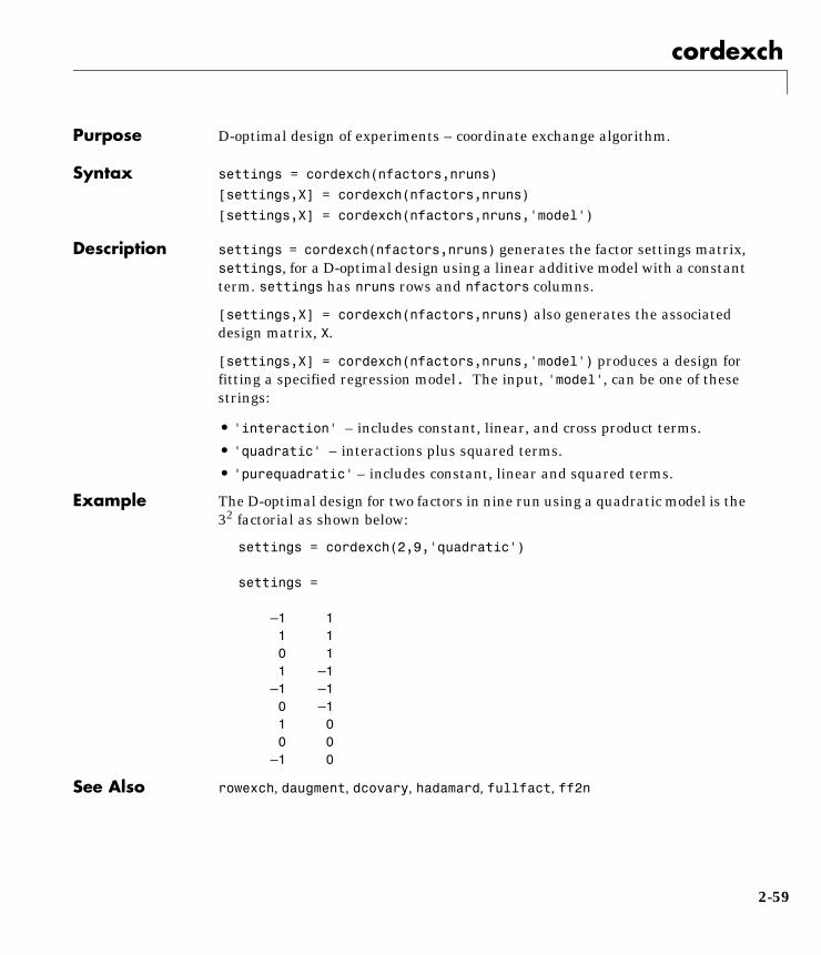
cordexch
2cordexchPurpose D-optimal design of experiments – coordinate exchange algorithm.
Syntax settings = cordexch(nfactors,nruns)
[settings,X] = cordexch(nfactors,nruns)
[settings,X] = cordexch(nfactors,nruns,'model')
Description settings = cordexch(nfactors,nruns) generates the factor settings matrix,settings, for a D-optimal design using a linear additive model with a constantterm. settings has nruns rows and nfactors columns.
[settings,X] = cordexch(nfactors,nruns) also generates the associateddesign matrix, X.
[settings,X] = cordexch(nfactors,nruns,'model') produces a design forfitting a specified regression model. The input, 'model', can be one of thesestrings:
• 'interaction' – includes constant, linear, and cross product terms.
• 'quadratic' – interactions plus squared terms.
• 'purequadratic' – includes constant, linear and squared terms.
Example The D-optimal design for two factors in nine run using a quadratic model is the32 factorial as shown below:
settings = cordexch(2,9,'quadratic')
settings =
–1 1 1 1 0 1 1 –1 –1 –1 0 –1 1 0 0 0 –1 0
See Also rowexch, daugment, dcovary, hadamard, fullfact, ff2n
2-59

corrcoef
2corrcoefPurpose Correlation coefficients.
Syntax R = corrcoef(X)
Description R = corrcoef(X) returns a matrix of correlation coefficients calculated froman input matrix whose rows are observations and whose columns are variables.The element (i,j) of the matrix R is related to the corresponding element ofthe covariance matrix C = cov(X) by
See Also cov, mean, std, var
corrcoef is a function in MATLAB.
rR i j,( ) C i j ),( )C i i,( )C j j,( )
-------------------------------------=
2-60
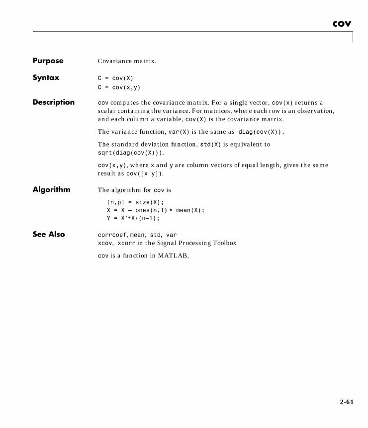
cov
2covPurpose Covariance matrix.
Syntax C = cov(X)
C = cov(x,y)
Description cov computes the covariance matrix. For a single vector, cov(x) returns ascalar containing the variance. For matrices, where each row is an observation,and each column a variable, cov(X) is the covariance matrix.
The variance function, var(X) is the same as diag(cov(X)).
The standard deviation function, std(X) is equivalent tosqrt(diag(cov(X))).
cov(x,y), where x and y are column vectors of equal length, gives the sameresult as cov([x y]).
Algorithm The algorithm for cov is
[n,p] = size(X);X = X – ones(n,1) * mean(X);Y = X'∗X/(n–1);
See Also corrcoef, mean, std, varxcov, xcorr in the Signal Processing Toolbox
cov is a function in MATLAB.
2-61
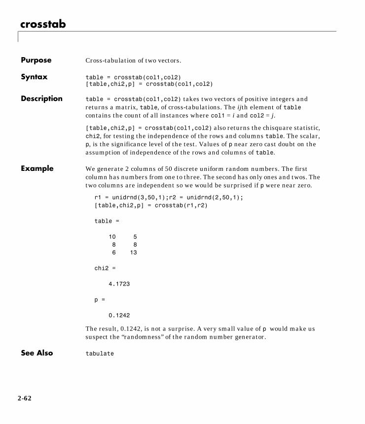
crosstab
2crosstabPurpose Cross-tabulation of two vectors.
Syntax table = crosstab(col1,col2)[table,chi2,p] = crosstab(col1,col2)
Description table = crosstab(col1,col2) takes two vectors of positive integers andreturns a matrix, table, of cross-tabulations. The ijth element of tablecontains the count of all instances where col1 = i and col2 = j.
[table,chi2,p] = crosstab(col1,col2) also returns the chisquare statistic,chi2, for testing the independence of the rows and columns table. The scalar,p, is the significance level of the test. Values of p near zero cast doubt on theassumption of independence of the rows and columns of table.
Example We generate 2 columns of 50 discrete uniform random numbers. The firstcolumn has numbers from one to three. The second has only ones and twos. Thetwo columns are independent so we would be surprised if p were near zero.
r1 = unidrnd(3,50,1);r2 = unidrnd(2,50,1);[table,chi2,p] = crosstab(r1,r2)
table =
10 5 8 8 6 13
chi2 =
4.1723
p =
0.1242
The result, 0.1242, is not a surprise. A very small value of p would make ussuspect the “randomness” of the random number generator.
See Also tabulate
2-62
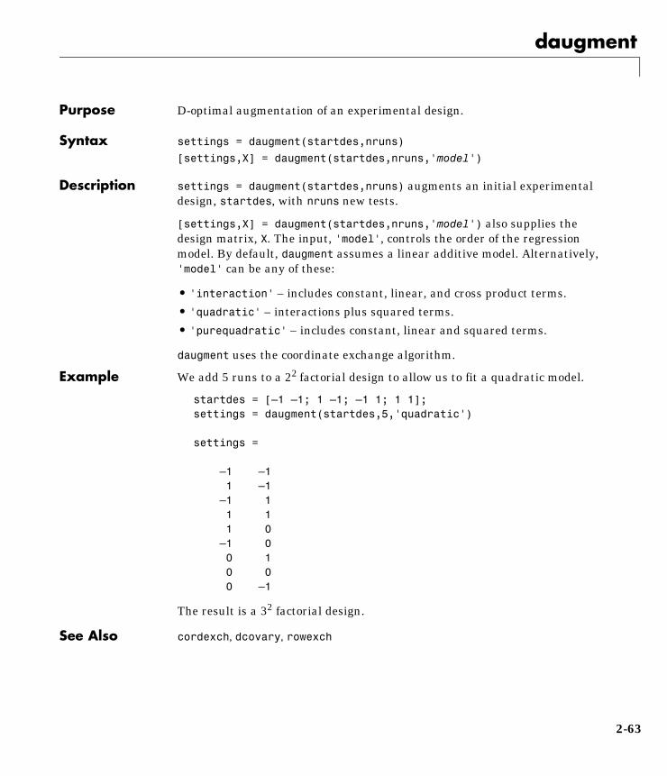
daugment
2daugmentPurpose D-optimal augmentation of an experimental design.
Syntax settings = daugment(startdes,nruns)
[settings,X] = daugment(startdes,nruns,'model')
Description settings = daugment(startdes,nruns) augments an initial experimentaldesign, startdes, with nruns new tests.
[settings,X] = daugment(startdes,nruns,'model') also supplies thedesign matrix, X. The input, 'model', controls the order of the regressionmodel. By default, daugment assumes a linear additive model. Alternatively,'model' can be any of these:
• 'interaction' – includes constant, linear, and cross product terms.
• 'quadratic' – interactions plus squared terms.
• 'purequadratic' – includes constant, linear and squared terms.
daugment uses the coordinate exchange algorithm.
Example We add 5 runs to a 22 factorial design to allow us to fit a quadratic model.
startdes = [–1 –1; 1 –1; –1 1; 1 1];settings = daugment(startdes,5,'quadratic')
settings =
–1 –1 1 –1 –1 1 1 1 1 0 –1 0 0 1 0 0 0 –1
The result is a 32 factorial design.
See Also cordexch, dcovary, rowexch
2-63

dcovary
2dcovaryPurpose D-optimal design with specified fixed covariates.
Syntax settings = dcovary(factors,covariates)
[settings,X] = dcovary(factors,covariates,'model')
Description settings = dcovary(factors,covariates,'model') creates a D-optimaldesign subject to the constraint of fixed covariates for each run. factors isthe number of experimental variables you want to control.
[settings,X] = dcovary(factors,covariates,'model') also creates theassociated design matrix, X. The input, 'model', controls the order of theregression model. By default, dcovary assumes a linear additive model.Alternatively, 'model' can be any of these:
• 'interaction' – includes constant, linear, and cross product terms.
• 'quadratic' – interactions plus squared terms.
• 'purequadratic' – includes constant, linear and squared terms.
Example Suppose we want to block an eight run experiment into 4 blocks of size 2 to fita linear model on two factors.
covariates = dummyvar([1 1 2 2 3 3 4 4]);settings = dcovary(2,covariates(:,1:3),'linear')settings =
1 1 1 0 0 –1 –1 1 0 0 –1 1 0 1 0 1 –1 0 1 0 1 1 0 0 1 –1 –1 0 0 1 –1 1 0 0 0 1 –1 0 0 0
The first two columns of the output matrix contain the settings for the twofactors. The last three columns are dummy variable codings for the four blocks.
See Also daugment, cordexch
2-64
dendrogram
2dendrogramPurpose Plot dendrogram graphs.
Syntax H = dendrogram(Z) H = dendrogram(Z,p)[H,T] = dendrogram(...)
Description H = dendrogram(Z) generates a dendrogram plot of the hierarchical, binarycluster tree, Z. Z is an m-1 by 3 matrix, generated by the linkage function,where m is the number of objects in the original dataset.
A dendrogram consists of many upside-down, U-shaped lines connectingobjects in a hierarchical tree. Except for the Ward linkage (see linkage), theheight of each U represents the distance between the two objects beingconnected. The output, H, is a vector of line handles.
H = dendrogram(Z,p) generates a dendrogram with only the top p nodes. Bydefault, dendrogram uses 30 as the value of p. When there are more than 30initial nodes, a dendrogram may look crowded. To display every node, set p = 0.
[H,T] = dendrogram(...) generates a dendrogram, returning T, a vector ofsize m that contains the cluster number for each object in the original dataset.T provides access to the nodes of a cluster hierarchy that are not displayed inthe dendrogram because they fall below the cutoff value p. For example, to findout which objects are contained in leaf node k of the dendrogram, usefind(T==k). Leaf nodes are the nodes at the bottom of the dendrogram thathave no other nodes below them.
When there are fewer than p objects in the original data, all objects aredisplayed in the dendrogram. In this case, T is the identical map, i.e.,T = (1:m)', where each node contains only itself.
2-65

dendrogram
Example rand('seed',12); X= rand(100,2); Y= pdist(X,'citiblock'); Z= linkage(Y,'average'); [H, T] = dendrogram(Z);
find(T==20)
ans =
204962657396
0
0.1
0.2
0.3
0.4
0.5
0.6
0.7
14 17 13 22 12 8 23 20 19 1 21 15 5 2 3 16 27 4 18 24 28 6 10 7 30 26 9 25 11 29
2-66

dendrogram
This output indicates that leaf node 20 in the dendrogram contains the originaldata points 20, 49, 62, 65, 73, and 96.
See Also cluster, clusterdata, cophenet, inconsistent, linkage, pdist, squareform
2-67
disttool
2disttoolPurpose Interactive graph of cdf (or pdf) for many probability distributions.
Syntax disttool
Description The disttool command sets up a graphic user interface for exploring theeffects of changing parameters on the plot of a cdf or pdf. Clicking and dragginga vertical line on the plot allows you to evaluate the function over its entiredomain interactively.
Evaluate the plotted function by typing a value in the x-axis edit box ordragging the vertical reference line on the plot. For cdfs, you can evaluate theinverse function by typing a value in the y-axis edit box or dragging thehorizontal reference line on the plot. The shape of the pointer changes from anarrow to a crosshair when you are over the vertical or horizontal line to indicatethat the reference line is draggable.
To change the distribution function choose from the pop-up menu of functionsat the top left of the figure. To change from cdfs to pdfs, choose from the pop-upmenu at the top right of the figure.
To change the parameter settings move the sliders or type a value in the editbox under the name of the parameter. To change the limits of a parameter, typea value in the edit box at the top or bottom of the parameter slider.
When you are done, press the Close button.
See Also randtool
2-68
dummyvar
2dummyvarPurpose Matrix of 0-1 “dummy” variables.
Syntax D = dummyvar(group)
Description D = dummyvar(group) generates a matrix, D, of 0-1 columns. D has one columnfor each unique value in each column of the matrix group. Each column ofgroup contains positive integers that indicate the group membership of anindividual row.
Example Suppose we are studying the effects of two machines and three operators on aprocess. The first column of group would have the values one or two dependingon which machine was used. The second column of groupwould have the valuesone, two, or three depending on which operator ran the machine.
group = [1 1;1 2;1 3;2 1;2 2;2 3];D = dummyvar(group)
D =
1 0 1 0 0 1 0 0 1 0 1 0 0 0 1 0 1 1 0 0 0 1 0 1 0 0 1 0 0 1
See Also pinv, regress
2-69
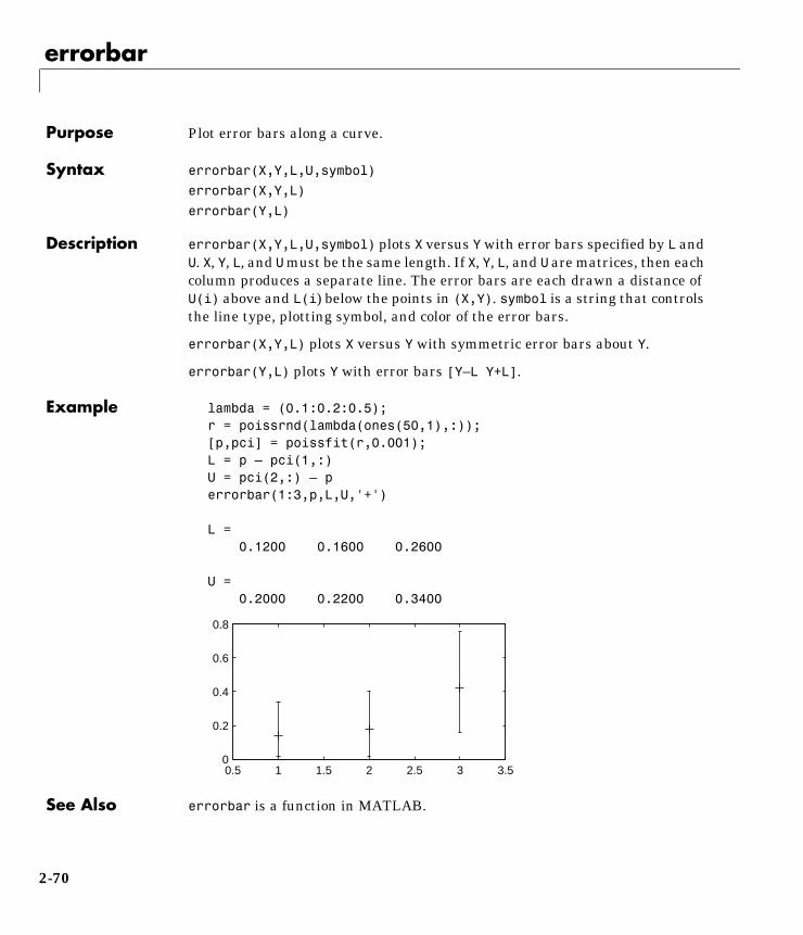
errorbar
2errorbarPurpose Plot error bars along a curve.
Syntax errorbar(X,Y,L,U,symbol)
errorbar(X,Y,L)
errorbar(Y,L)
Description errorbar(X,Y,L,U,symbol) plots X versus Y with error bars specified by L andU. X, Y, L, and U must be the same length. If X, Y, L, and U are matrices, then eachcolumn produces a separate line. The error bars are each drawn a distance ofU(i) above and L(i) below the points in (X,Y). symbol is a string that controlsthe line type, plotting symbol, and color of the error bars.
errorbar(X,Y,L) plots X versus Y with symmetric error bars about Y.
errorbar(Y,L) plots Y with error bars [Y–L Y+L].
Example lambda = (0.1:0.2:0.5);r = poissrnd(lambda(ones(50,1),:));[p,pci] = poissfit(r,0.001);L = p – pci(1,:) U = pci(2,:) – perrorbar(1:3,p,L,U,'+')
L = 0.1200 0.1600 0.2600
U = 0.2000 0.2200 0.3400
See Also errorbar is a function in MATLAB.
0.5 1 1.5 2 2.5 3 3.50
0.2
0.4
0.6
0.8
2-70
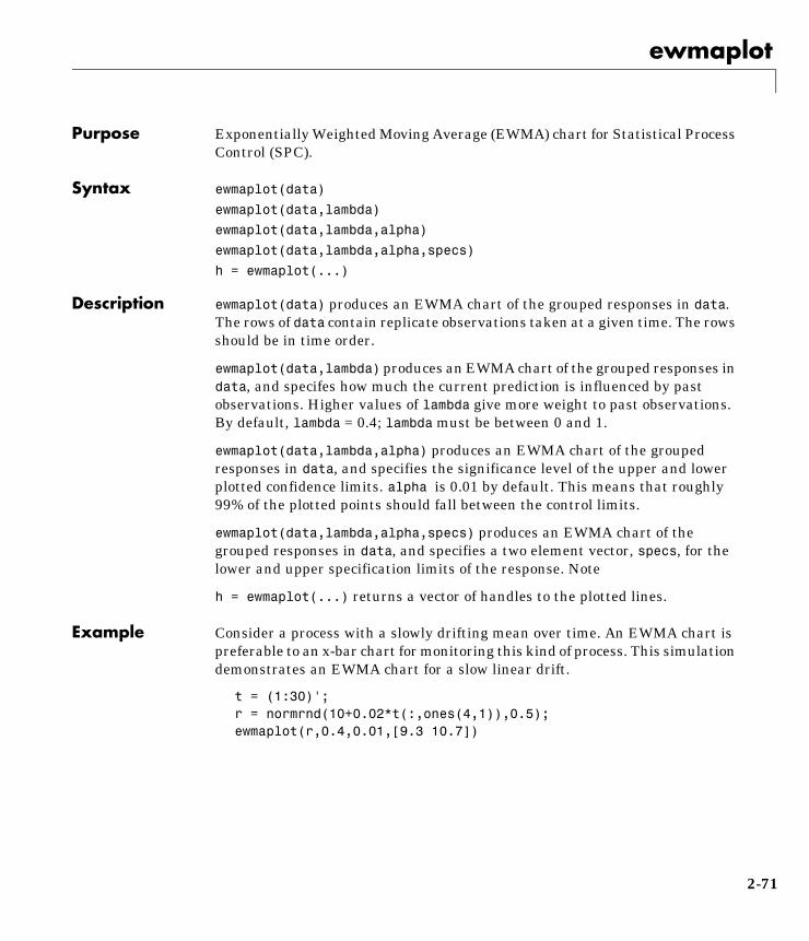
ewmaplot
2ewmaplotPurpose Exponentially Weighted Moving Average (EWMA) chart for Statistical ProcessControl (SPC).
Syntax ewmaplot(data)
ewmaplot(data,lambda)
ewmaplot(data,lambda,alpha)
ewmaplot(data,lambda,alpha,specs)
h = ewmaplot(...)
Description ewmaplot(data) produces an EWMA chart of the grouped responses in data.The rows of data contain replicate observations taken at a given time. The rowsshould be in time order.
ewmaplot(data,lambda) produces an EWMA chart of the grouped responses indata, and specifes how much the current prediction is influenced by pastobservations. Higher values of lambda give more weight to past observations.By default, lambda = 0.4; lambda must be between 0 and 1.
ewmaplot(data,lambda,alpha) produces an EWMA chart of the groupedresponses in data, and specifies the significance level of the upper and lowerplotted confidence limits. alpha is 0.01 by default. This means that roughly99% of the plotted points should fall between the control limits.
ewmaplot(data,lambda,alpha,specs) produces an EWMA chart of thegrouped responses in data, and specifies a two element vector, specs, for thelower and upper specification limits of the response. Note
h = ewmaplot(...) returns a vector of handles to the plotted lines.
Example Consider a process with a slowly drifting mean over time. An EWMA chart ispreferable to an x-bar chart for monitoring this kind of process. This simulationdemonstrates an EWMA chart for a slow linear drift.
t = (1:30)';r = normrnd(10+0.02*t(:,ones(4,1)),0.5);ewmaplot(r,0.4,0.01,[9.3 10.7])
2-71
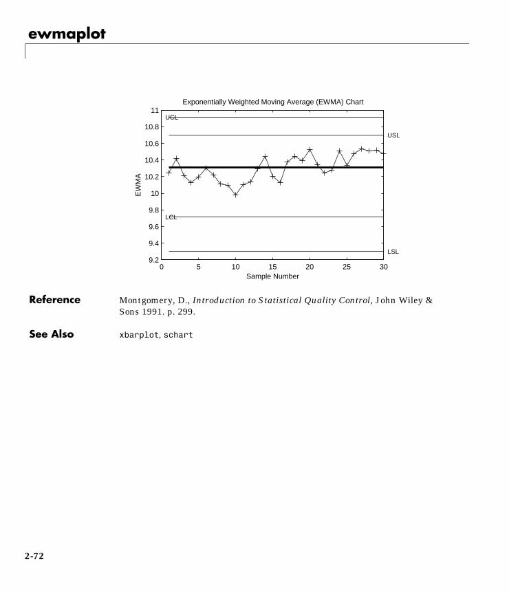
ewmaplot
Reference Montgomery, D., Introduction to Statistical Quality Control, John Wiley &Sons 1991. p. 299.
See Also xbarplot, schart
0 5 10 15 20 25 309.2
9.4
9.6
9.8
10
10.2
10.4
10.6
10.8
11UCL
LCL
Exponentially Weighted Moving Average (EWMA) Chart
USL
LSL
Sample Number
EW
MA
2-72
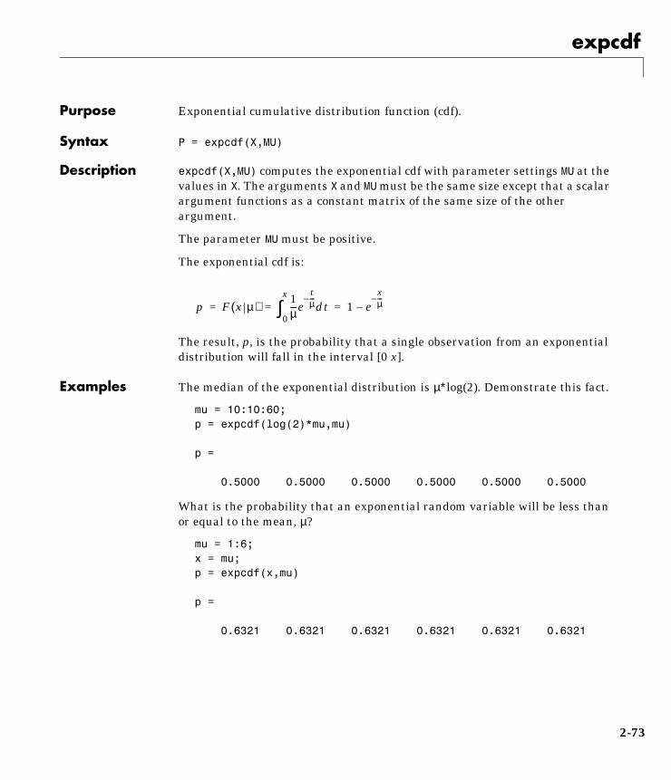
expcdf
2expcdfPurpose Exponential cumulative distribution function (cdf).
Syntax P = expcdf(X,MU)
Description expcdf(X,MU) computes the exponential cdf with parameter settings MU at thevalues in X. The arguments X and MU must be the same size except that a scalarargument functions as a constant matrix of the same size of the otherargument.
The parameter MU must be positive.
The exponential cdf is:
The result, p, is the probability that a single observation from an exponentialdistribution will fall in the interval [0 x].
Examples The median of the exponential distribution is µ∗log(2). Demonstrate this fact.
mu = 10:10:60; p = expcdf(log(2)*mu,mu)
p =
0.5000 0.5000 0.5000 0.5000 0.5000 0.5000
What is the probability that an exponential random variable will be less thanor equal to the mean, µ?
mu = 1:6;x = mu;p = expcdf(x,mu)
p =
0.6321 0.6321 0.6321 0.6321 0.6321 0.6321
p F x µ( )1µ---e
tµ---–
0
x
∫ dt 1 exµ---–
–= = =
2-73

expfit
2expfitPurpose Parameter estimates and confidence intervals for exponential data.
Syntax muhat = expfit(x)
[muhat,muci] = expfit(x)
[muhat,muci] = expfit(x,alpha)
Description muhat = expfit(x) returns the estimate of the parameter, µ, of theexponential distribution given the data, x.
[muhat,muci] = expfit(x) also returns the 95% confidence interval inmuci.
[muhat,muci] = expfit(x,alpha) gives 100(1–alpha) percent confidenceintervals. For example, alpha = 0.01 yields 99% confidence intervals.
Example We generate 100 independent samples of exponential data with µ = 3. muhat isan estimate of true_mu and muci is a 99% confidence interval aroundmuhat. Notice that muci contains true_mu.
true_mu = 3;[muhat,muci] = expfit(r,0.01)
muhat =
2.8835
muci =
2.1949 3.6803
See Also betafit, binofit, gamfit, normfit, poissfit, unifit, weibfit
2-74
expinv
2expinvPurpose Inverse of the exponential cumulative distribution function (cdf).
Syntax X = expinv(P,MU)
Description expinv(P,MU) computes the inverse of the exponential cdf with parameter MUfor the probabilities in P. The arguments P and MU must be the same size exceptthat a scalar argument functions as a constant matrix of the size of the otherargument.
The parameter MU must be positive and P must lie on the interval [0 1].
The inverse of the exponential cdf is:
The result, x, is the value such that the probability is p that an observationfrom an exponential distribution with parameter µ will fall in the range [0 x].
Examples Let the lifetime of light bulbs be exponentially distributed with mu equal to 700hours. What is the median lifetime of a bulb?
expinv(0.50,700)
ans =
485.2030
So, suppose you buy a box of “700 hour” light bulbs. If 700 hours is mean life ofthe bulbs, then half them will burn out in less than 500 hours.
x F p µ( ) µln 1 p–( )–= =
2-75
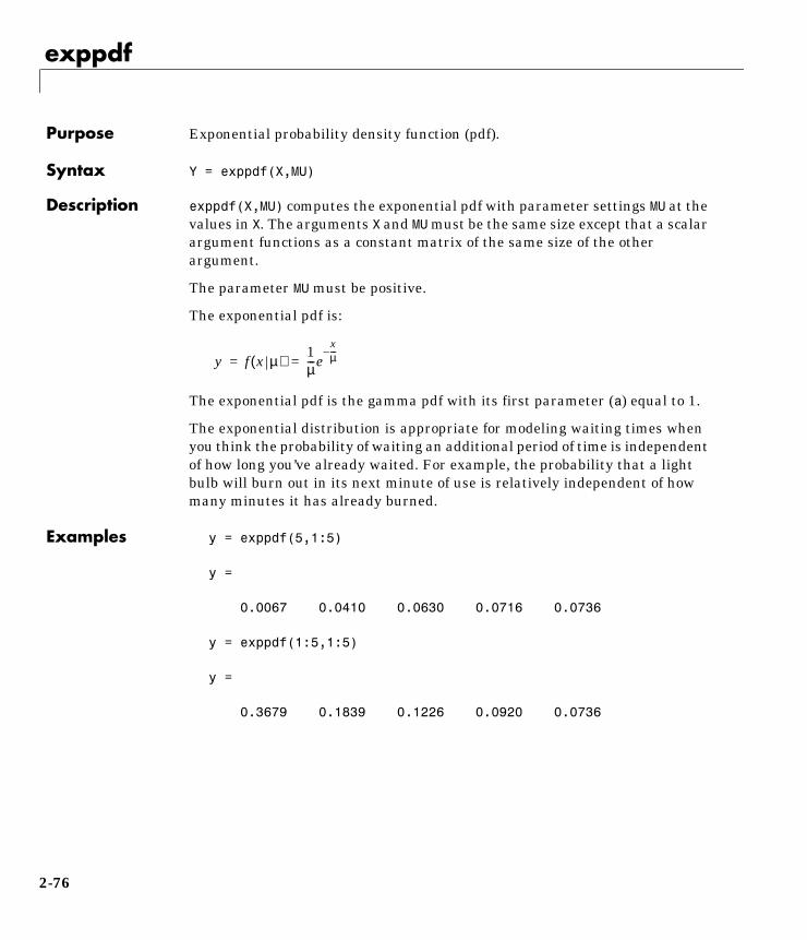
exppdf
2exppdfPurpose Exponential probability density function (pdf).
Syntax Y = exppdf(X,MU)
Description exppdf(X,MU) computes the exponential pdf with parameter settings MU at thevalues in X. The arguments X and MU must be the same size except that a scalarargument functions as a constant matrix of the same size of the otherargument.
The parameter MU must be positive.
The exponential pdf is:
The exponential pdf is the gamma pdf with its first parameter (a) equal to 1.
The exponential distribution is appropriate for modeling waiting times whenyou think the probability of waiting an additional period of time is independentof how long you’ve already waited. For example, the probability that a lightbulb will burn out in its next minute of use is relatively independent of howmany minutes it has already burned.
Examples y = exppdf(5,1:5)
y =
0.0067 0.0410 0.0630 0.0716 0.0736
y = exppdf(1:5,1:5)
y =
0.3679 0.1839 0.1226 0.0920 0.0736
y f x µ( )1µ---e
xµ---–
= =
2-76

exprnd
2exprndPurpose Random numbers from the exponential distribution.
Syntax R = exprnd(MU)R = exprnd(MU,m)R = exprnd(MU,m,n)
Description R = exprnd(MU) generates exponential random numbers with mean MU. Thesize of R is the size of MU.
R = exprnd(MU,m) generates exponential random numbers with mean MU. m isa 1-by-2 vector that contains the row and column dimensions of R.
R = exprnd(MU,m,n) generates exponential random numbers with mean MU.The scalars m and n are the row and column dimensions of R.
Examples n1 = exprnd(5:10)
n1 =
7.5943 18.3400 2.7113 3.0936 0.6078 9.5841
n2 = exprnd(5:10,[1 6])
n2 =
3.2752 1.1110 23.5530 23.4303 5.7190 3.9876
n3 = exprnd(5,2,3)
n3 =
24.3339 13.5271 1.8788 4.7932 4.3675 2.6468
2-77
expstat
2expstatPurpose Mean and variance for the exponential distribution.
Syntax [M,V] = expstat(MU)
Description For the exponential distribution:
• The mean is µ.
• The variance is µ2.
Examples [m,v] = expstat([1 10 100 1000])
m =
1 10 100 1000
v =
1 100 10000 1000000
2-78
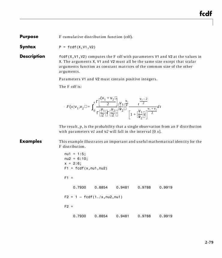
fcdf
2fcdfPurpose F cumulative distribution function (cdf).
Syntax P = fcdf(X,V1,V2)
Description fcdf(X,V1,V2) computes the F cdf with parameters V1 and V2 at the values inX. The arguments X, V1 and V2 must all be the same size except that scalararguments function as constant matrices of the common size of the otherarguments.
Parameters V1 and V2 must contain positive integers.
The F cdf is:
The result, p, is the probability that a single observation from an F distributionwith parameters ν1 and ν2 will fall in the interval [0 x].
Examples This example illustrates an important and useful mathematical identity for theF distribution.
nu1 = 1:5;nu2 = 6:10;x = 2:6;F1 = fcdf(x,nu1,nu2)
F1 =
0.7930 0.8854 0.9481 0.9788 0.9919
F2 = 1 – fcdf(1./x,nu2,nu1)
F2 =
0.7930 0.8854 0.9481 0.9788 0.9919
F x ν1 ν2,( )Γ
ν1 ν2+( )2-----------------------
Γν12------
Γν22------
--------------------------------
0
x
∫ν1ν2------
ν1
2----- tν1 2–
2--------------
1ν1ν2------
t+
ν1 ν2+2-----------------
------------------------------------------dt= =
2-79

ff2n
2ff2nPurpose Two-level full-factorial designs.
Syntax X = ff2n(n)
Description X = ff2n(n) creates a two-level full-factorial design, X. n is the number ofcolumns of X. The number of rows is 2n.
Example X = ff2n(3)
X =
0 0 0 0 0 1 0 1 0 0 1 1 1 0 0 1 0 1 1 1 0 1 1 1
X is the binary representation of the numbers from 0 to 2n–1.
See Also fullfact
2-80

finv
2finvPurpose Inverse of the F cumulative distribution function (cdf).
Syntax X = finv(P,V1,V2)
Description finv(P,V1,V2) computes the inverse of the F cdf with numerator degrees offreedom,V1, and denominator degrees of freedom, V2, for the probabilities inP. The arguments P, V1 and V2 must all be the same size except that scalararguments function as constant matrices of the common size of the otherarguments.
The parameters V1 and V2 must both be positive integers and P must lie on theinterval [0 1].
The F inverse function is defined in terms of the F cdf:
Examples Find a value that should exceed 95% of the samples from an F distribution with5 degrees of freedom in the numerator and 10 degrees of freedom in thedenominator.
x = finv(0.95,5,10)
x =
3.3258
You would observe values greater than 3.3258 only 5% of the time by chance.
x F 1– p ν1 ν2,( ) x:F x ν1 ν2,( ) p={ }= =
where p F x ν1 ν2,( )Γ
ν1 ν2+( )2-----------------------
Γν12------
Γν22------
--------------------------------
0
x
∫ν1ν2------
ν1
2----- tν1 2–
2--------------
1ν1ν2------
t+
ν1 ν2+2-----------------
------------------------------------------dt= =
2-81

fpdf
2fpdfPurpose F probability density function (pdf).
Syntax Y = fpdf(X,V1,V2)
Description fpdf(X,V1,V2) computes the F pdf with parameters V1 and V2 at the values inX. The arguments X, V1 and V2 must all be the same size except that scalararguments function as constant matrices of the common size of the otherarguments.
The parameters V1 and V2 must both be positive integers and X must lie on theinterval [0 ∞).
The probability density function for the F distribution is:
Examples y = fpdf(1:6,2,2)
y =
0.2500 0.1111 0.0625 0.0400 0.0278 0.0204
z = fpdf(3,5:10,5:10)
z =
0.0689 0.0659 0.0620 0.0577 0.0532 0.0487
y f x ν1 ν2,( )Γ
ν1 ν2+( )2-----------------------
Γν12------
Γν22------
--------------------------------
ν1ν2------
ν1
2----- xν1 2–
2--------------
1ν1ν2------
x+
ν1 ν2+2-----------------
-------------------------------------------= =
2-82

frnd
2frndPurpose Random numbers from the F distribution.
Syntax R = frnd(V1,V2)
R = frnd(V1,V2,m)
R = frnd(V1,V2,m,n)
Description R = frnd(V1,V2) generates random numbers from the F distribution withnumerator degrees of freedom, V1, and denominator degrees of freedom, V2.The size of R is the common size of V1 and V2 if both are matrices. If eitherparameter is a scalar, the size of R is the size of the other parameter.
R = frnd(V1,V2,m) generates random numbers from the F distribution withparameters V1 and V2. m is a 1-by-2 vector that contains the row and columndimensions of R.
R = frnd(V1,V2,m,n) generates random numbers from the F distribution withparameters V1 and V2. The scalars m and n are the row and column dimensionsof R.
Examples n1 = frnd(1:6,1:6)
n1 =
0.0022 0.3121 3.0528 0.3189 0.2715 0.9539
n2 = frnd(2,2,[2 3])
n2 =
0.3186 0.9727 3.0268 0.2052 148.5816 0.2191
n3 = frnd([1 2 3;4 5 6],1,2,3)
n3 =
0.6233 0.2322 31.5458 2.5848 0.2121 4.4955
2-83

fstat
2fstatPurpose Mean and variance for the F distribution.
Syntax [M,V] = fstat(V1,V2)
Description For the F distribution:
• The mean, for values of n2 greater than 2, is:
• The variance, for values of n greater than 4, is:
The mean of the F distribution is undefined if ν2 is less than 3. The variance isundefined for ν2 less than 5.
Examples fstat returns NaN when the mean and variance are undefined.
[m,v] = fstat(1:5,1:5)
m =
NaN NaN 3.0000 2.0000 1.6667
v =
NaN NaN NaN NaN 8.8889
ν2ν2 2–------------
2ν22 ν1 ν2 2–+( )
ν1 ν2 2–( )2 ν2 4–( )--------------------------------------------------
2-84

fsurfht
2fsurfhtPurpose Interactive contour plot of a function.
Syntax fsurfht('fun',xlims,ylims)
fsurfht('fun',xlims,ylims,p1,p2,p3,p4,p5)
Description fsurfht('fun',xlims,ylims) is an interactive contour plot of the functionspecified by the text variable fun. The x-axis limits are specified by xlims =[xmin xmax] and the y-axis limits specified by ylims.
fsurfht('fun',xlims,ylims,p1,p2,p3,p4,p5) allows for five optionalparameters that you can supply to the function 'fun'. The first two argumentsof fun are the x-axis variable and y-axis variable, respectively.
There are vertical and horizontal reference lines on the plot whose intersectiondefines the current x-value and y-value. You can drag these dotted whitereference lines and watch the calculated z-values (at the top of the plot) updatesimultaneously. Alternatively, you can get a specific z-value by typing thex-value and y-value into editable text fields on the x-axis and y-axisrespectively.
Example Plot the Gaussian likelihood function for the gas.mat data.
load gas
Write the M-file, gauslike.m.
function z = gauslike(mu,sigma,p1)n = length(p1);z = ones(size(mu));for i = 1:nz = z .* (normpdf(p1(i),mu,sigma));end
2-85
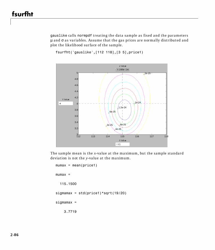
fsurfht
gauslike calls normpdf treating the data sample as fixed and the parametersµ and σ as variables. Assume that the gas prices are normally distributed andplot the likelihood surface of the sample.
fsurfht('gauslike',[112 118],[3 5],price1)
The sample mean is the x-value at the maximum, but the sample standarddeviation is not the y-value at the maximum.
mumax = mean(price1)
mumax =
115.1500
sigmamax = std(price1)*sqrt(19/20)
sigmamax =
3.7719
112 113 114 115 116 117 1183
3.2
3.4
3.6
3.8
4
4.2
4.4
4.6
4.8
5
2e-25
2e-25
4e-25
6e-25
8e-25
1e-24
1.2e-24
2-86
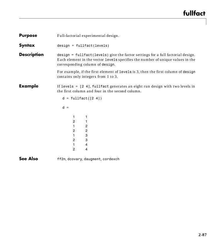
fullfact
2fullfactPurpose Full-factorial experimental design.
Syntax design = fullfact(levels)
Description design = fullfact(levels) give the factor settings for a full factorial design.Each element in the vector levels specifies the number of unique values in thecorresponding column of design.
For example, if the first element of levels is 3, then the first column of designcontains only integers from 1 to 3.
Example If levels = [2 4], fullfact generates an eight run design with two levels inthe first column and four in the second column.
d = fullfact([2 4])
d =
1 1 2 1 1 2 2 2 1 3 2 3 1 4 2 4
See Also ff2n, dcovary, daugment, cordexch
2-87
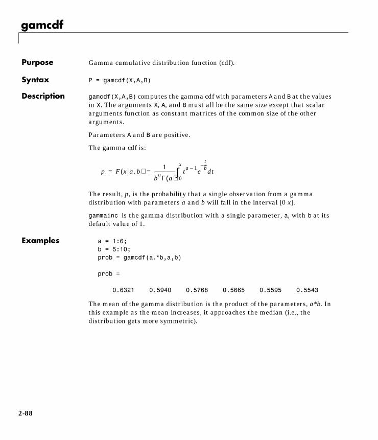
gamcdf
2gamcdfPurpose Gamma cumulative distribution function (cdf).
Syntax P = gamcdf(X,A,B)
Description gamcdf(X,A,B) computes the gamma cdf with parameters A and B at the valuesin X. The arguments X, A, and B must all be the same size except that scalararguments function as constant matrices of the common size of the otherarguments.
Parameters A and B are positive.
The gamma cdf is:
The result, p, is the probability that a single observation from a gammadistribution with parameters a and b will fall in the interval [0 x].
gammainc is the gamma distribution with a single parameter, a, with b at itsdefault value of 1.
Examples a = 1:6;b = 5:10;prob = gamcdf(a.∗b,a,b)
prob =
0.6321 0.5940 0.5768 0.5665 0.5595 0.5543
The mean of the gamma distribution is the product of the parameters, a*b. Inthis example as the mean increases, it approaches the median (i.e., thedistribution gets more symmetric).
p F x a b,( ) 1
baΓ a( )------------------ ta 1– e
tb---–
td0
x
∫= =
2-88

gamfit
2gamfitPurpose Parameter estimates and confidence intervals for gamma distributed data.
Syntax phat = gamfit(x)
[phat,pci] = gamfit(x)
[phat,pci] = gamfit(x,alpha)
Description phat = gamfit(x) returns the maximum likelihood estimates of theparameters of the gamma distribution given the data in the vector, x.
[phat,pci] = gamfit(x) gives MLEs and 95% percent confidence intervals.The first row of pci is the lower bound of the confidence intervals; the last rowis the upper bound.
[phat,pci] = gamfit(x,alpha) returns 100(1–alpha) percent confidenceintervals. For example, alpha = 0.01 yields 99% confidence intervals.
Example Note the 95% confidence intervals in the example bracket the “true” parametervalues, 2 and 4, respectively.
a = 2; b = 4;r = gamrnd(a,b,100,1);[p,ci] = gamfit(r)
p =
2.1990 3.7426
ci =
1.6840 2.8298 2.7141 4.6554
Reference Hahn, G. J., and S.S. Shapiro, Statistical Models in Engineering, WileyClassics Library John Wiley & Sons, New York. 1994. p. 88.
See Also betafit, binofit, expfit, normfit, poissfit, unifit, weibfit
2-89
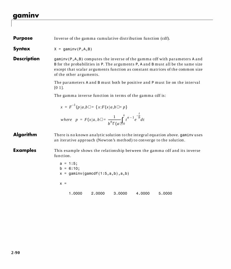
gaminv
2gaminvPurpose Inverse of the gamma cumulative distribution function (cdf).
Syntax X = gaminv(P,A,B)
Description gaminv(P,A,B) computes the inverse of the gamma cdf with parameters A andB for the probabilities in P. The arguments P, A and B must all be the same sizeexcept that scalar arguments function as constant matrices of the common sizeof the other arguments.
The parameters A and B must both be positive and P must lie on the interval[0 1].
The gamma inverse function in terms of the gamma cdf is:
Algorithm There is no known analytic solution to the integral equation above. gaminv usesan iterative approach (Newton’s method) to converge to the solution.
Examples This example shows the relationship between the gamma cdf and its inversefunction.
a = 1:5;b = 6:10;x = gaminv(gamcdf(1:5,a,b),a,b)
x =
1.0000 2.0000 3.0000 4.0000 5.0000
x F 1– p a b,( ) x:F x a b,( ) p={ }= =
where p F x a b,( )1
baΓ a( )------------------ ta 1– e
tb---–
td0
x
∫= =
2-90
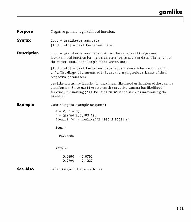
gamlike
2gamlikePurpose Negative gamma log-likelihood function.
Syntax logL = gamlike(params,data)
[logL,info] = gamlike(params,data)
Description logL = gamlike(params,data) returns the negative of the gammalog-likelihood function for the parameters, params, given data. The length ofthe vector, logL, is the length of the vector, data.
[logL,info] = gamlike(params,data) adds Fisher's information matrix,info. The diagonal elements of info are the asymptotic variances of theirrespective parameters.
gamlike is a utility function for maximum likelihood estimation of the gammadistribution. Since gamlike returns the negative gamma log-likelihoodfunction, minimizing gamlike using fmins is the same as maximizing thelikelihood.
Example Continuing the example for gamfit:
a = 2; b = 3;r = gamrnd(a,b,100,1);[logL,info] = gamlike([2.1990 2.8069],r)
logL =
267.5585
info =
0.0690 –0.0790 –0.0790 0.1220
See Also betalike, gamfit, mle, weiblike
2-91

gampdf
2gampdfPurpose Gamma probability density function (pdf).
Syntax Y = gampdf(X,A,B)
Description gampdf(X,A,B) computes the gamma pdf with parameters A and B at the valuesin X. The arguments X, A and B must all be the same size except that scalararguments function as constant matrices of the common size of the otherarguments.
The parameters A and B must both be positive and X must lie on the interval[0 ∞).
The gamma pdf is:
Gamma probability density function is useful in reliability models of lifetimes.The gamma distribution is more flexible than the exponential in that theprobability of surviving an additional period may depend on age. Special casesof the gamma function are the exponential and χ2 functions.
Examples The exponential distribution is a special case of the gamma distribution.
mu = 1:5;y = gampdf(1,1,mu)
y =
0.3679 0.3033 0.2388 0.1947 0.1637
y1 = exppdf(1,mu)
y1 =
0.3679 0.3033 0.2388 0.1947 0.1637
y f x a b,( )1
baΓ a( )------------------xa 1– e
xb---–
= =
2-92

gamrnd
2gamrndPurpose Random numbers from the gamma distribution.
Syntax R = gamrnd(A,B)
R = gamrnd(A,B,m)
R = gamrnd(A,B,m,n)
Description R = gamrnd(A,B) generates gamma random numbers with parameters A andB. The size of R is the common size of A and B if both are matrices. If eitherparameter is a scalar, the size of R is the size of the other parameter.
R = gamrnd(A,B,m) generates gamma random numbers with parameters A andB. m is a 1-by-2 vector that contains the row and column dimensions of R.
R = gamrnd(A,B,m,n) generates gamma random numbers with parameters Aand B. The scalars m and n are the row and column dimensions of R.
Examples n1 = gamrnd(1:5,6:10)
n1 =
9.1132 12.8431 24.8025 38.5960 106.4164
n2 = gamrnd(5,10,[1 5])
n2 =
30.9486 33.5667 33.6837 55.2014 46.8265
n3 = gamrnd(2:6,3,1,5)
n3 =
12.8715 11.3068 3.0982 15.6012 21.6739
2-93
gamstat
2gamstatPurpose Mean and variance for the gamma distribution.
Syntax [M,V] = gamstat(A,B)
Description For the gamma distribution:
• The mean is ab.
• The variance is ab2.
Examples [m,v] = gamstat(1:5,1:5)
m =
1 4 9 16 25
v =
1 8 27 64 125
[m,v] = gamstat(1:5,1./(1:5))
m =
1 1 1 1 1
v =
1.0000 0.5000 0.3333 0.2500 0.2000
2-94
geocdf
2geocdfPurpose Geometric cumulative distribution function (cdf).
Syntax Y = geocdf(X,P)
Description geocdf(X,P) computes the geometric cdf with probabilities, P, at the values inX. The arguments X and P must be the same size except that a scalar argumentfunctions as a constant matrix of the same size as the other argument.
The parameter, P, is on the interval [0 1].
The geometric cdf is:
where:
The result, y, is the probability of observing up to x trials before a success whenthe probability of success in any given trial is p.
Examples Suppose you toss a fair coin repeatedly. If the coin lands face up (heads), thatis a success. What is the probability of observing three or fewer tails beforegetting a heads?
p = geocdf(3,0.5)
p =
0.9375
y F x p( ) pqi
i 0=
floorx
∑= =
q 1 p–=
2-95
geoinv
2geoinvPurpose Inverse of the geometric cumulative distribution function (cdf).
Syntax X = geoinv(Y,P)
Description geoinv(Y,P) returns the smallest integer X such that the geometric cdfevaluated at X is equal to or exceeds Y. You can think of Y as the probability ofobserving X successes in a row in independent trials where P is the probabilityof success in each trial.
The arguments P and Y must lie on the interval [0 1]. Each X is a positiveinteger.
Examples The probability of correctly guessing the result of 10 coin tosses in a row is lessthan 0.001 (unless the coin is not fair.)
psychic = geoinv(0.999,0.5)
psychic =
9
The example below shows the inverse method for generating random numbersfrom the geometric distribution.
rndgeo = geoinv(rand(2,5),0.5)
rndgeo =
0 1 3 1 0 0 1 0 2 0
2-96
geomean
2geomeanPurpose Geometric mean of a sample.
Syntax m = geomean(X)
Description geomean calculates the geometric mean of a sample. For vectors, geomean(x) isthe geometric mean of the elements in x. For matrices, geomean(X) is a rowvector containing the geometric means of each column.
The geometric mean is:
Examples The sample average is greater than or equal to the geometric mean.
x = exprnd(1,10,6);geometric = geomean(x)
geometric =
0.7466 0.6061 0.6038 0.2569 0.7539 0.3478
average = mean(x)
average =
1.3509 1.1583 0.9741 0.5319 1.0088 0.8122
See Also mean, median, harmmean, trimmean
m xi
i 1=
n
∏1n---
=
2-97
geopdf
2geopdfPurpose Geometric probability density function (pdf).
Syntax Y = geopdf(X,P)
Description geocdf(X,P) computes the geometric pdf with probabilities, P, at the values inX. The arguments X and P must be the same size except that a scalar argumentfunctions as a constant matrix of the same size as the other argument.
The parameter, P, is on the interval [0 1].
The geometric pdf is:
where:
Examples Suppose you toss a fair coin repeatedly. If the coin lands face up (heads), thatis a success. What is the probability of observing exactly three tails beforegetting a heads?
p = geopdf(3,0.5)
p =
0.0625
y f x p( ) pqxI 0 1 K, ,( ) x( )= =
q 1 p–=
2-98

geornd
2georndPurpose Random numbers from the geometric distribution.
Syntax R = geornd(P)
R = geornd(P,m)
R = geornd(P,m,n)
Description The geometric distribution is useful when you want to model the number offailed trials in a row before a success where the probability of success in anygiven trial is the constant P.
R = geornd(P) generates geometric random numbers with probabilityparameter, P . The size of R is the size of P.
R = geornd(P,m) generates geometric random numbers with probabilityparameter, P. m is a 1-by-2 vector that contains the row and column dimensionsof R.
R = geornd(P,m,n) generates geometric random numbers with probabilityparameter, P. The scalars m and n are the row and column dimensions of R.
The parameter P must lie on the interval [0 1].
Examples r1 = geornd(1 ./ 2.^(1:6))r1 =
2 10 2 5 2 60
r2 = geornd(0.01,[1 5])
r2 =
65 18 334 291 63
r3 = geornd(0.5,1,6)
r3 =
0 7 1 3 1 0
2-99
geostat
2geostatPurpose Mean and variance for the geometric distribution.
Syntax [M,V] = geostat(P)
Description For the geometric distribution:
• The mean is .
• The variance is .
where q = 1– p.
Examples [m,v] = geostat(1./(1:6))
m =
0 1.0000 2.0000 3.0000 4.0000 5.0000
v =
0 2.0000 6.0000 12.0000 20.0000 30.0000
qp---
q
p2------
2-100
gline
2glinePurpose Interactively draw a line in a figure.
Syntax gline(fig)
h = gline(fig)
gline
Description gline(fig) draws a line segment by clicking the mouse at the two end-pointsof the line segment in the figure, fig. A rubber band line tracks the mousemovement.
h = gline(fig) returns the handle to the line in h.
gline with no input arguments draws in the current figure.
See Also refline, gname
2-101
gname
2gnamePurpose Label plotted points with their case names or case number.
Syntax gname('cases')gnameh = gname('cases',line_handle)
Description gname('cases') displays the graph window, puts up a cross-hair, and waits fora mouse button or keyboard key to be pressed. Position the cross-hair with themouse and click once near each point that you want to label. When you aredone, press the Return or Enter key and the labels will appear at each pointthat you clicked. 'cases' is a string matrix. Each row is the case name of a datapoint.
gname with no arguments labels each case with its case number.
h = gname(cases,line_handle) returns a vector of handles to the text objectson the plot. Use the scalar, line_handle, to identify the correct line if there ismore than one line object on the plot.
Example Let’s use the city ratings datasets to find out which cities are the best and worstfor education and the arts.
2-102

gname
load citieseducation = ratings(:,6); arts = ratings(:,7);plot(education,arts,'+')gname(names)
See Also gtext
1500 2000 2500 3000 3500 40000
1
2
3
4
5
6x 10⁴
Pascagoula, MS
New York, NY
2-103
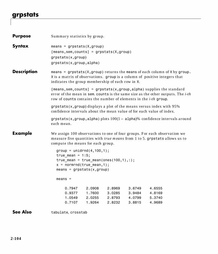
grpstats
2grpstatsPurpose Summary statistics by group.
Syntax means = grpstats(X,group)
[means,sem,counts] = grpstats(X,group)
grpstats(x,group)grpstats(x,group,alpha)
Description means = grpstats(X,group) returns the means of each column of X by group.X is a matrix of observations. group is a column of positive integers thatindicates the group membership of each row in X.
[means,sem,counts] = grpstats(x,group,alpha) supplies the standarderror of the mean in sem. counts is the same size as the other outputs. The i-throw of counts contains the number of elements in the i-th group.
grpstats(x,group) displays a plot of the means versus index with 95%confidence intervals about the mean value of for each value of index.
grpstats(x,group,alpha) plots 100(1 – alpha)% confidence intervals aroundeach mean.
Example We assign 100 observations to one of four groups. For each observation wemeasure five quantities with true means from 1 to 5. grpstats allows us tocompute the means for each group.
group = unidrnd(4,100,1);true_mean = 1:5;true_mean = true_mean(ones(100,1),:);x = normrnd(true_mean,1);means = grpstats(x,group)
means =
0.7947 2.0908 2.8969 3.6749 4.6555 0.9377 1.7600 3.0285 3.9484 4.8169 1.0549 2.0255 2.8793 4.0799 5.3740 0.7107 1.9264 2.8232 3.8815 4.9689
See Also tabulate, crosstab
2-104
harmmean
2harmmeanPurpose Harmonic mean of a sample of data.
Syntax m = harmmean(X)
Description harmmean calculates the harmonic mean of a sample. For vectors,harmmean(x) is the harmonic mean of the elements in x. For matrices,harmmean(X) is a row vector containing the harmonic means of each column.
The harmonic mean is:
Examples The sample average is greater than or equal to the harmonic mean.
x = exprnd(1,10,6);harmonic = harmmean(x)
harmonic =
0.3382 0.3200 0.3710 0.0540 0.4936 0.0907
average = mean(x)
average =
1.3509 1.1583 0.9741 0.5319 1.0088 0.8122
See Also mean, median, geomean, trimmean
mn
1xi----
i 1=
n
∑---------------=
2-105
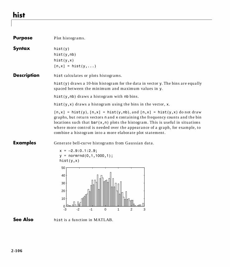
hist
2histPurpose Plot histograms.
Syntax hist(y)
hist(y,nb)
hist(y,x)
[n,x] = hist(y,...)
Description hist calculates or plots histograms.
hist(y) draws a 10-bin histogram for the data in vector y. The bins are equallyspaced between the minimum and maximum values in y.
hist(y,nb) draws a histogram with nb bins.
hist(y,x) draws a histogram using the bins in the vector, x.
[n,x] = hist(y), [n,x] = hist(y,nb), and [n,x] = hist(y,x) do not drawgraphs, but return vectors n and x containing the frequency counts and the binlocations such that bar(x,n) plots the histogram. This is useful in situationswhere more control is needed over the appearance of a graph, for example, tocombine a histogram into a more elaborate plot statement.
Examples Generate bell-curve histograms from Gaussian data.
x = –2.9:0.1:2.9;y = normrnd(0,1,1000,1);hist(y,x)
See Also hist is a function in MATLAB.
-3 -2 -1 0 1 2 30
10
20
30
40
50
2-106
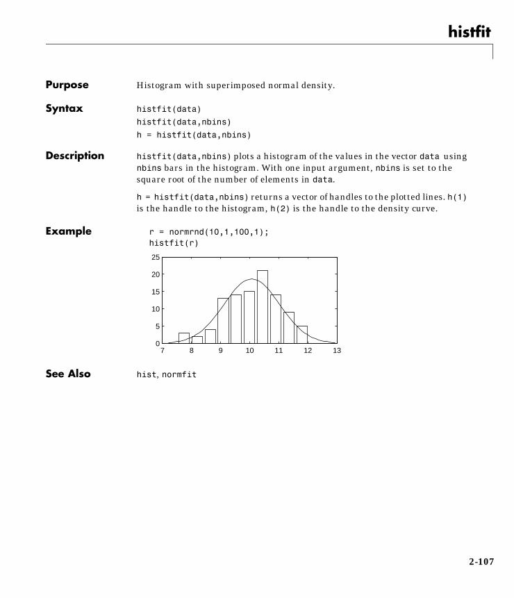
histfit
2histfitPurpose Histogram with superimposed normal density.
Syntax histfit(data)
histfit(data,nbins)
h = histfit(data,nbins)
Description histfit(data,nbins) plots a histogram of the values in the vector data usingnbins bars in the histogram. With one input argument, nbins is set to thesquare root of the number of elements in data.
h = histfit(data,nbins) returns a vector of handles to the plotted lines. h(1)is the handle to the histogram, h(2) is the handle to the density curve.
Example r = normrnd(10,1,100,1);histfit(r)
See Also hist, normfit
7 8 9 10 11 12 130
5
10
15
20
25
2-107
hougen
2hougenPurpose Hougen-Watson model for reaction kinetics.
Syntax yhat = hougen(beta,X)
Description yhat = hougen(beta,x) gives the predicted values of the reaction rate, yhat,as a function of the vector of parameters, beta, and the matrix of data, X. betamust have 5 elements and X must have three columns.
hougen is a utility function for rsmdemo.
The model form is:
Reference Bates, D., and D. Watts, Nonlinear Regression Analysis and Its Applications,Wiley 1988. p. 271–272.
See Also rsmdemo
yβ1x2 x3 β5⁄–
1 β2x1 β3x2 β4x3+ + +-----------------------------------------------------------=
2-108
hygecdf
2hygecdfPurpose Hypergeometric cumulative distribution function (cdf).
Syntax P = hygecdf(X,M,K,N)
Description hygecdf(X,M,K,N) computes the hypergeometric cdf with parameters M, K, andN at the values in X. The arguments X, M, K, and N must all be the same sizeexcept that scalar arguments function as constant matrices of the common sizeof the other arguments.
The hypergeometric cdf is:
The result, p, is the probability of drawing up to x items of a possible K in Ndrawings without replacement from a group of M objects.
Examples Suppose you have a lot of 100 floppy disks and you know that 20 of them aredefective. What is the probability of drawing zero to two defective floppies ifyou select 10 at random?
p = hygecdf(2,100,20,10)
p =
0.6812
p F x M K N, ,( )
Ki
M K–
N i–
MN
------------------------------
i 0=
x
∑= =
2-109

hygeinv
2hygeinvPurpose Inverse of the hypergeometric cumulative distribution function (cdf).
Syntax X = hygeinv(P,M,K,N)
Description hygeinv(P,M,K,N) returns the smallest integer X such that the hypergeometriccdf evaluated at X equals or exceeds P. You can think of P as the probability ofobserving X defective items in N drawings without replacement from a group ofM items where K are defective.
Examples Suppose you are the Quality Assurance manager of a floppy diskmanufacturer. The production line turns out floppy disks in batches of 1,000.You want to sample 50 disks from each batch to see if they have defects. Youwant to accept 99% of the batches if there are no more than 10 defective disksin the batch. What is the maximum number of defective disks should you allowin your sample of 50?
x = hygeinv(0.99,1000,10,50)
x =
3
What is the median number of defective floppy disks in samples of 50 disksfrom batches with 10 defective disks?
x = hygeinv(0.50,1000,10,50)
x =
0
2-110
hygepdf
2hygepdfPurpose Hypergeometric probability density function (pdf).
Syntax Y = hygepdf(X,M,K,N)
Description hygecdf(X,M,K,N) computes the hypergeometric pdf with parameters M, K, andN at the values in X. The arguments X, M, K, and N must all be the same sizeexcept that scalar arguments function as constant matrices of the common sizeof the other arguments.
The parameters M, K, and N must be positive integers. Also X must be less thanor equal to all the parameters and N must be less than or equal to M.
The hypergeometric pdf is:
The result, y, is the probability of drawing exactly x items of a possible K in ndrawings without replacement from group of M objects.
Examples Suppose you have a lot of 100 floppy disks and you know that 20 of them aredefective. What is the probability of drawing 0 through 5 defective floppy disksif you select 10 at random?
p = hygepdf(0:5,100,20,10)
p =
0.0951 0.2679 0.3182 0.2092 0.0841 0.0215
y f x M K N, ,( )
Kx
M K–
N x–
MN
------------------------------= =
2-111
hygernd
2hygerndPurpose Random numbers from the hypergeometric distribution.
Syntax R = hygernd(M,K,N)
R = hygernd(M,K,N,mm)
R = hygernd(M,K,N,mm,nn)
Description R = hygernd(M,K,N) generates hypergeometric random numbers withparameters M,K and N. The size of R is the common size of M, K, and N if all arematrices. If any parameter is a scalar, the size of R is the common size of thenonscalar parameters.
R = hygernd(M,K,N,mm) generates hypergeometric random numbers withparameters M, K, and N. mm is a 1-by-2 vector that contains the row and columndimensions of R.
R = hygernd(M,K,N,mm,nn) generates hypergeometric random numbers withparameters M, K, and N. The scalars mm and nn are the row and columndimensions of R.
Examples numbers = hygernd(1000,40,50)
numbers =
1
2-112
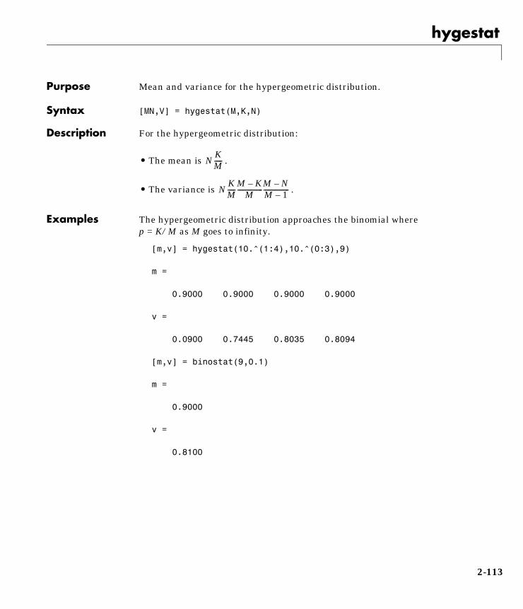
hygestat
2hygestatPurpose Mean and variance for the hypergeometric distribution.
Syntax [MN,V] = hygestat(M,K,N)
Description For the hypergeometric distribution:
• The mean is .
• The variance is .
Examples The hypergeometric distribution approaches the binomial wherep = K/M as M goes to infinity.
[m,v] = hygestat(10.^(1:4),10.^(0:3),9)
m =
0.9000 0.9000 0.9000 0.9000
v =
0.0900 0.7445 0.8035 0.8094
[m,v] = binostat(9,0.1)
m =
0.9000
v =
0.8100
NKM-----
NKM-----
M K–M----------------
M N–M 1–----------------
2-113
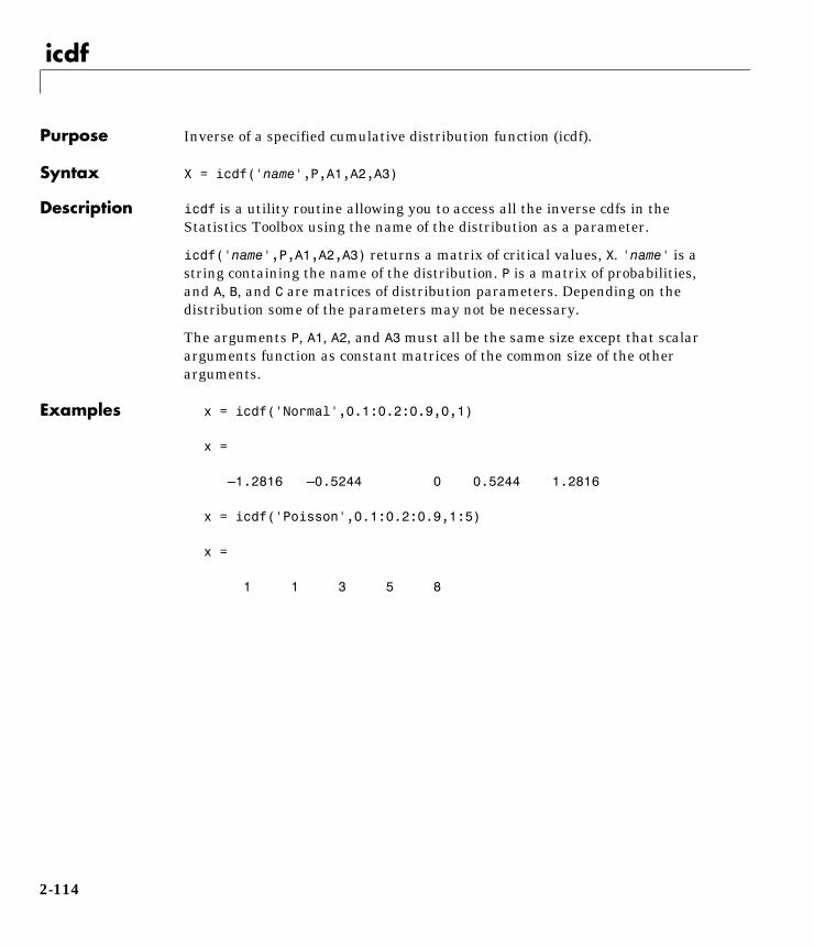
icdf
2icdfPurpose Inverse of a specified cumulative distribution function (icdf).
Syntax X = icdf('name',P,A1,A2,A3)
Description icdf is a utility routine allowing you to access all the inverse cdfs in theStatistics Toolbox using the name of the distribution as a parameter.
icdf('name',P,A1,A2,A3) returns a matrix of critical values, X. 'name' is astring containing the name of the distribution. P is a matrix of probabilities,and A, B, and C are matrices of distribution parameters. Depending on thedistribution some of the parameters may not be necessary.
The arguments P, A1, A2, and A3 must all be the same size except that scalararguments function as constant matrices of the common size of the otherarguments.
Examples x = icdf('Normal',0.1:0.2:0.9,0,1)
x =
–1.2816 –0.5244 0 0.5244 1.2816
x = icdf('Poisson',0.1:0.2:0.9,1:5)
x =
1 1 3 5 8
2-114
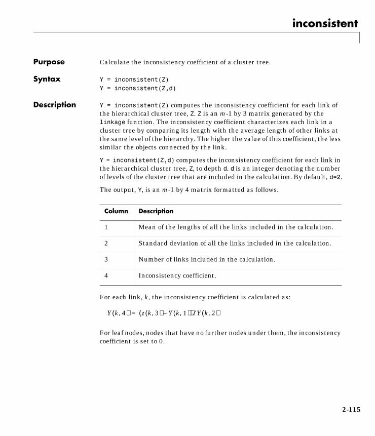
inconsistent
2inconsistentPurpose Calculate the inconsistency coefficient of a cluster tree.
Syntax Y = inconsistent(Z) Y = inconsistent(Z,d)
Description Y = inconsistent(Z) computes the inconsistency coefficient for each link ofthe hierarchical cluster tree, Z. Z is an m-1 by 3 matrix generated by thelinkage function. The inconsistency coefficient characterizes each link in acluster tree by comparing its length with the average length of other links atthe same level of the hierarchy. The higher the value of this coefficient, the lesssimilar the objects connected by the link.
Y = inconsistent(Z,d) computes the inconsistency coefficient for each link inthe hierarchical cluster tree, Z, to depth d. d is an integer denoting the numberof levels of the cluster tree that are included in the calculation. By default, d=2.
The output, Y, is an m-1 by 4 matrix formatted as follows.
For each link, k, the inconsistency coefficient is calculated as:
For leaf nodes, nodes that have no further nodes under them, the inconsistencycoefficient is set to 0.
Column Description
1 Mean of the lengths of all the links included in the calculation.
2 Standard deviation of all the links included in the calculation.
3 Number of links included in the calculation.
4 Inconsistency coefficient.
Y k 4,( ) z k 3,( ) Y k 1,( )–( ) Y k 2,( )⁄=
2-115
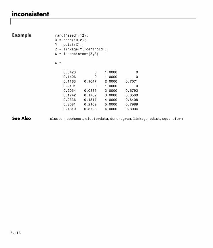
inconsistent
Example rand('seed',12);X = rand(10,2);Y = pdist(X);Z = linkage(Y,'centroid');W = inconsistent(Z,3)
W =
0.0423 0 1.0000 0 0.1406 0 1.0000 0 0.1163 0.1047 2.0000 0.70710.2101 0 1.0000 00.2054 0.0886 3.0000 0.67920.1742 0.1762 3.0000 0.65680.2336 0.1317 4.0000 0.64080.3081 0.2109 5.0000 0.79890.4610 0.3728 4.0000 0.8004
See Also cluster, cophenet, clusterdata, dendrogram, linkage, pdist, squareform
2-116
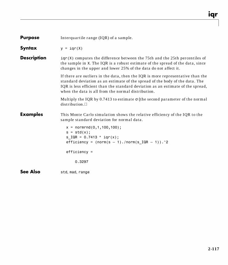
iqr
2iqrPurpose Interquartile range (IQR) of a sample.
Syntax y = iqr(X)
Description iqr(X) computes the difference between the 75th and the 25th percentiles ofthe sample in X. The IQR is a robust estimate of the spread of the data, sincechanges in the upper and lower 25% of the data do not affect it.
If there are outliers in the data, then the IQR is more representative than thestandard deviation as an estimate of the spread of the body of the data. TheIQR is less efficient than the standard deviation as an estimate of the spread,when the data is all from the normal distribution.
Multiply the IQR by 0.7413 to estimate σ (the second parameter of the normaldistribution.)
Examples This Monte Carlo simulation shows the relative efficiency of the IQR to thesample standard deviation for normal data.
x = normrnd(0,1,100,100);s = std(x);s_IQR = 0.7413 ∗ iqr(x);efficiency = (norm(s – 1)./norm(s_IQR – 1)).^2
efficiency =
0.3297
See Also std, mad, range
2-117

kurtosis
2kurtosisPurpose Sample kurtosis.
Syntax k = kurtosis(X)
Description k = kurtosis(X) returns the sample kurtosis of X. For vectors,kurtosis(x) is the kurtosis of the elements in the vector, x. For matriceskurtosis(X) returns the sample kurtosis for each column of X.
Kurtosis is a measure of how outlier-prone a distribution is. The kurtosis of thenormal distribution is 3. Distributions that are more outlier-prone than thenormal distribution have kurtosis greater than 3; distributions that are lessoutlier-prone have kurtosis less than 3.
The kurtosis of a distribution is defined as
where E(x) is the expected value of x.
Note: Some definitions of kurtosis subtract 3 from the computed value, so thatthe normal distribution has kurtosis of 0. The kurtosis function does not usethis convention.
Example X = randn([5 4])
X =
1.1650 1.6961 –1.4462 –0.3600 0.6268 0.0591 –0.7012 –0.1356 0.0751 1.7971 1.2460 –1.3493 0.3516 0.2641 –0.6390 –1.2704 –0.6965 0.8717 0.5774 0.9846
k = kurtosis(X)
k =
2.1658 1.2967 1.6378 1.9589
See Also mean, moment, skewness, std, var
kE x µ–( )4
σ4------------------------=
2-118
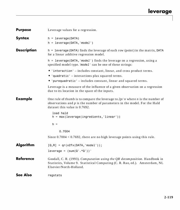
leverage
2leveragePurpose Leverage values for a regression.
Syntax h = leverage(DATA)
h = leverage(DATA,'model')
Description h = leverage(DATA) finds the leverage of each row (point) in the matrix, DATAfor a linear additive regression model.
h = leverage(DATA,'model') finds the leverage on a regression, using aspecified model type. 'model' can be one of these strings:
• 'interaction' – includes constant, linear, and cross product terms.
• 'quadratic' – interactions plus squared terms.
• 'purequadratic' – includes constant, linear and squared terms.
Leverage is a measure of the influence of a given observation on a regressiondue to its location in the space of the inputs.
Example One rule of thumb is to compare the leverage to 2p/n where n is the number ofobservations and p is the number of parameters in the model. For the Halddataset this value is 0.7692.
load haldh = max(leverage(ingredients,'linear'))
h =
0.7004
Since 0.7004 < 0.7692, there are no high leverage points using this rule.
Algorithm [Q,R] = qr(x2fx(DATA,'model'));
leverage = (sum(Q'.*Q'))'
Reference Goodall, C. R. (1993). Computation using the QR decomposition. Handbook inStatistics, Volume 9. Statistical Computing (C. R. Rao, ed.). Amsterdam, NLElsevier/North-Holland.
See Also regstats
2-119
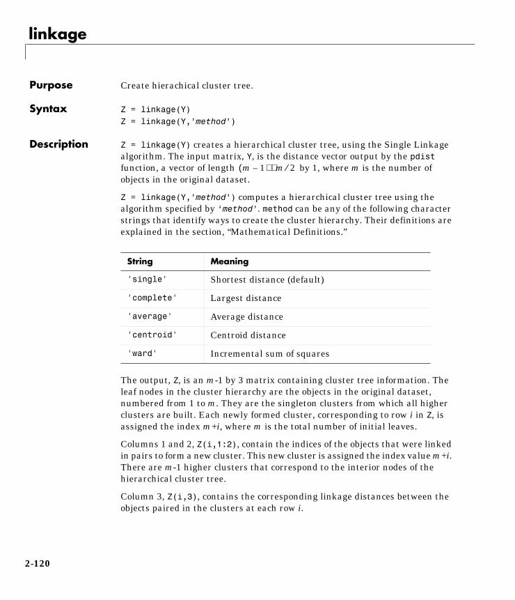
linkage
2linkagePurpose Create hierachical cluster tree.
Syntax Z = linkage(Y) Z = linkage(Y,’method’)
Description Z = linkage(Y) creates a hierarchical cluster tree, using the Single Linkagealgorithm. The input matrix, Y, is the distance vector output by the pdistfunction, a vector of length by 1, where m is the number ofobjects in the original dataset.
Z = linkage(Y,’method’) computes a hierarchical cluster tree using thealgorithm specified by ‘method’. method can be any of the following characterstrings that identify ways to create the cluster hierarchy. Their definitions areexplained in the section, “Mathematical Definitions.”
The output, Z, is an m-1 by 3 matrix containing cluster tree information. Theleaf nodes in the cluster hierarchy are the objects in the original dataset,numbered from 1 to m. They are the singleton clusters from which all higherclusters are built. Each newly formed cluster, corresponding to row i in Z, isassigned the index m+i, where m is the total number of initial leaves.
Columns 1 and 2, Z(i,1:2), contain the indices of the objects that were linkedin pairs to form a new cluster. This new cluster is assigned the index value m+i.There are m-1 higher clusters that correspond to the interior nodes of thehierarchical cluster tree.
Column 3, Z(i,3), contains the corresponding linkage distances between theobjects paired in the clusters at each row i.
String Meaning
'single' Shortest distance (default)
'complete' Largest distance
'average' Average distance
'centroid' Centroid distance
'ward' Incremental sum of squares
m 1–( ) m 2⁄⋅
2-120
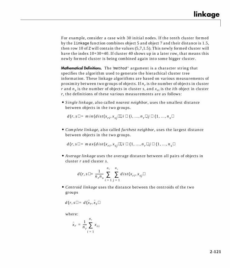
linkage
For example, consider a case with 30 initial nodes. If the tenth cluster formedby the linkage function combines object 5 and object 7 and their distance is 1.5,then row 10 of Z will contain the values (5,7,1.5). This newly formed cluster willhave the index 10+30=40. If cluster 40 shows up in a later row, that means thisnewly formed cluster is being combined again into some bigger cluster.
Mathematical Definitions. The ‘method’ argument is a character string thatspecifies the algorithm used to generate the hierachical cluster treeinformation. These linkage algorithms are based on various measurements ofproximity between two groups of objects. If nr is the number of objects in clusterr and ns is the number of objects in cluster s, and xri is the ith object in clusterr, the definitions of these various measurements are as follows:
• Single linkage, also called nearest neighbor, uses the smallest distancebetween objects in the two groups.
• Complete linkage, also called furthest neighbor, uses the largest distancebetween objects in the two groups.
• Average linkage uses the average distance between all pairs of objects incluster r and cluster s.
• Centroid linkage uses the distance between the centroids of the twogroups
where:
d r s,( ) min dist xri xsj,( )( ) i i … nr, ,( )∈ j 1 … ns, ,( )∈, ,=
d r s,( ) max dist xri xsj,( )( ) i 1 … nr, ,( )∈ j 1 … ns, ,( )∈, ,=
d r s,( )1
nrns------------ dist xri xsj,( )
j 1=
ns
∑i 1=
nr
∑=
d r s,( ) d xr xs,( )=
xr1nr------ xri
i 1=
nr
∑=
2-121

linkage
and is defined similarly.
• Ward linkage uses the incremental sum of squares; that is, the increase inthe total within-group sum of squares as a result of joining groups r and s. Itis given by
where is the distance between cluster r and cluster s defined in theCentroid linkage. The within-group sum of squares of a cluster is defined asthe sum of the squares of the distance between all objects in the cluster andthe centroid of the cluster.
Example X = [3 1.7; 1 1; 2 3; 2 2.5; 1.2 1; 1.1 1.5; 3 1];Y = pdist(x);Z = linkage(y)
Z =
2.0000 5.0000 0.20003.0000 4.0000 0.50008.0000 6.0000 0.50991.0000 7.0000 0.700011.0000 9.0000 1.280612.0000 10.0000 1.3454
See Also cluster, clusterdata, cophenet, dendrogram, inconsistent, pdist,squareform
xs
d r s,( ) nrnsdrs2 nr ns+( )⁄=
drs2
2-122

logncdf
2logncdfPurpose Lognormal cumulative distribution function.
Syntax P = logncdf(X,MU,SIGMA)
Description P = logncdf(X,MU,SIGMA) computes the lognormal cdf with mean MU andstandard deviation SIGMA at the values in X.
The size of P is the common size of X, MU and SIGMA. A scalar input functions asa constant matrix of the same size as the other inputs.
The lognormal cdf is:
Example x = (0:0.2:10);y = logncdf(x,0,1);plot(x,y);grid;xlabel('x');ylabel('p')
Reference Evans, M., N. Hastings, and B. Peacock, Statistical Distributions, SecondEdition, John Wiley and Sons, 1993. p. 102–105.
See Also cdf, logninv, lognpdf, lognrnd, lognstat
p F x µ σ,( )1
σ 2π--------------- e
ln t( ) µ–( )– 2
2σ2--------------------------------
t----------------------------- td0
x
∫= =
0 2 4 6 8 100
0.2
0.4
0.6
0.8
1
x
p
2-123
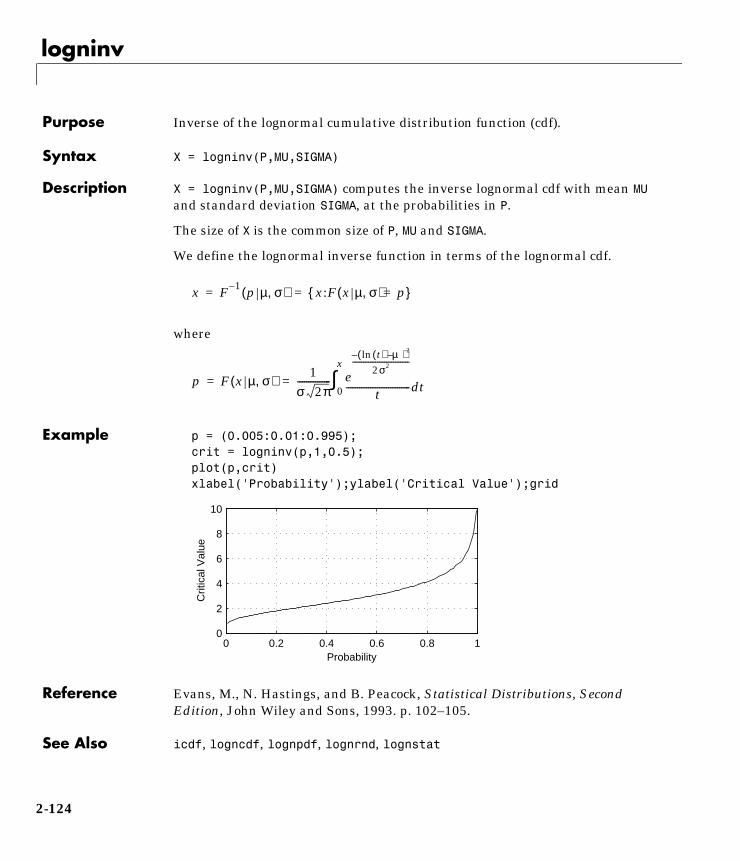
logninv
2logninvPurpose Inverse of the lognormal cumulative distribution function (cdf).
Syntax X = logninv(P,MU,SIGMA)
Description X = logninv(P,MU,SIGMA) computes the inverse lognormal cdf with mean MUand standard deviation SIGMA, at the probabilities in P.
The size of X is the common size of P, MU and SIGMA.
We define the lognormal inverse function in terms of the lognormal cdf.
where
Example p = (0.005:0.01:0.995);crit = logninv(p,1,0.5);plot(p,crit)xlabel('Probability');ylabel('Critical Value');grid
Reference Evans, M., N. Hastings, and B. Peacock, Statistical Distributions, SecondEdition, John Wiley and Sons, 1993. p. 102–105.
See Also icdf, logncdf, lognpdf, lognrnd, lognstat
x F 1– p µ σ,( ) x:F x µ σ,( ) p={ }= =
p F x µ σ,( )1
σ 2π--------------- e
ln t( ) µ–( )– 2
2σ2--------------------------------
t----------------------------- td0
x
∫= =
0 0.2 0.4 0.6 0.8 10
2
4
6
8
10
Probability
Crit
ical
Val
ue
2-124
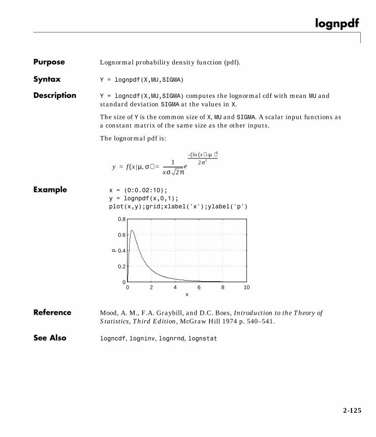
lognpdf
2lognpdfPurpose Lognormal probability density function (pdf).
Syntax Y = lognpdf(X,MU,SIGMA)
Description Y = logncdf(X,MU,SIGMA) computes the lognormal cdf with mean MU andstandard deviation SIGMA at the values in X.
The size of Y is the common size of X, MU and SIGMA. A scalar input functions asa constant matrix of the same size as the other inputs.
The lognormal pdf is:
Example x = (0:0.02:10);y = lognpdf(x,0,1);plot(x,y);grid;xlabel('x');ylabel('p')
Reference Mood, A. M., F.A. Graybill, and D.C. Boes, Introduction to the Theory ofStatistics, Third Edition, McGraw Hill 1974 p. 540–541.
See Also logncdf, logninv, lognrnd, lognstat
y f x µ σ,( )1
xσ 2π------------------e
ln x( ) µ–( )– 2
2σ2---------------------------------
= =
0 2 4 6 8 100
0.2
0.4
0.6
0.8
x
p
2-125
lognrnd
2lognrndPurpose Random matrices from the lognormal distribution.
Syntax R = lognrnd(MU,SIGMA)
R = lognrnd(MU,SIGMA,m)
R = lognrnd(MU,SIGMA,m,n)
Description R = lognrnd(MU,SIGMA) generates lognormal random numbers withparameters, MU and SIGMA. The size of R is the common size of MU and SIGMA ifboth are matrices. If either parameter is a scalar, the size of R is the size of theother parameter.
R = lognrnd(MU,SIGMA,m) generates lognormal random numbers withparameters MU and SIGMA. m is a 1-by-2 vector that contains the row and columndimensions of R.
R = lognrnd(MU,SIGMA,m,n) generates lognormal random numbers withparameters MU and SIGMA. The scalars m and n are the row and columndimensions of R.
Example r = lognrnd(0,1,4,3)
r =
3.2058 0.4983 1.3022 1.8717 5.4529 2.3909 1.0780 1.0608 0.2355 1.4213 6.0320 0.4960
Reference Evans, M., N. Hastings, and B. Peacock, Statistical Distributions, SecondEdition, John Wiley and Sons, 1993. p. 102–105.
See Also random, logncdf, logninv, lognpdf, lognstat
2-126
lognstat
2lognstatPurpose Mean and variance for the lognormal distribution.
Syntax [M,V] = lognstat(MU,SIGMA)
Description [M,V] = lognstat(MU,SIGMA) returns the mean and variance of the lognormaldistribution with parameters MU and SIGMA. The size of M and V is the commonsize of MU and SIGMA if both are matrices. If either parameter is a scalar, thesize of M and V is the size of the other parameter.
For the lognormal distribution, the mean is:
The variance is:
Example [m,v]= lognstat(0,1)
m =
1.6487
v =
7.0212
Reference Mood, A. M., F.A. Graybill, and D.C. Boes, Introduction to the Theory ofStatistics, Third Edition, McGraw Hill 1974 p. 540–541.
See Also logncdf, logninv, lognrnd, lognrnd
eµ σ2
2-----+
e 2µ 2σ2+( ) e 2µ σ2+( )–
2-127
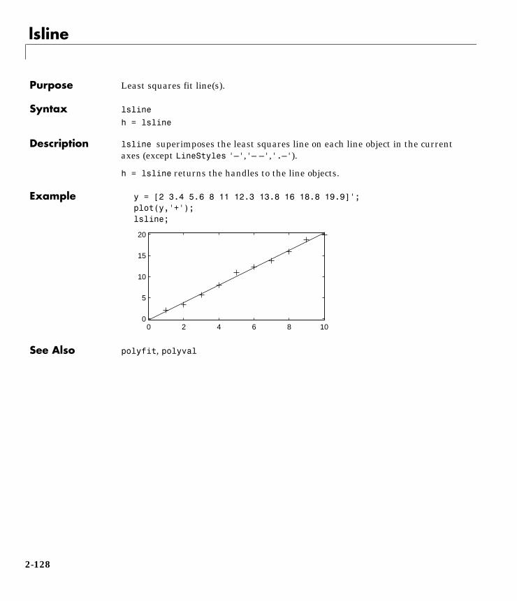
lsline
2lslinePurpose Least squares fit line(s).
Syntax lsline
h = lsline
Description lsline superimposes the least squares line on each line object in the currentaxes (except LineStyles '–','– –','.–').
h = lsline returns the handles to the line objects.
Example y = [2 3.4 5.6 8 11 12.3 13.8 16 18.8 19.9]';plot(y,'+');lsline;
See Also polyfit, polyval
0 2 4 6 8 100
5
10
15
20
2-128
mad
2madPurpose Mean absolute deviation (MAD) of a sample of data.
Syntax y = mad(X)
Description mad(X) computes the average of the absolute differences between a set of dataand the sample mean of that data. For vectors, mad(x) returns the meanabsolute deviation of the elements of x. For matrices, mad(X) returns the MADof each column of X.
The MAD is less efficient than the standard deviation as an estimate of thespread, when the data is all from the normal distribution.
Multiply the MAD by 1.3 to estimate σ (the second parameter of the normaldistribution).
Examples This example shows a Monte Carlo simulation of the relative efficiency of theMAD to the sample standard deviation for normal data.
x = normrnd(0,1,100,100);s = std(x);s_MAD = 1.3 ∗ mad(x);efficiency = (norm(s – 1)./norm(s_MAD – 1)).^2
efficiency =
0.5972
See Also std, range
2-129
mahal
2mahalPurpose Mahalanobis distance.
Syntax d = mahal(Y,X)
Description mahal(Y,X) computes the Mahalanobis distance of each point (row) of thematrix, Y, from the sample in the matrix, X.
The number of columns of Y must equal the number of columns in X, but thenumber of rows may differ. The number of rows in X must exceed the numberof columns.
The Mahalanobis distance is a multivariate measure of the separation of a dataset from a point in space. It is the criterion minimized in linear discriminantanalysis.
Example The Mahalanobis distance of a matrix, r, when applied to itself is a way to findoutliers.
r = mvnrnd([0 0],[1 0.9;0.9 1],100);r = [r;10 10];d = mahal(r,r);last6 = d(96:101)
last6 =
1.1036 2.2353 2.0219 0.3876 1.5571 52.7381
The last element is clearly an outlier.
See Also classify
2-130

mean
2meanPurpose Average or mean value of vectors and matrices.
Syntax m = mean(X)
Description mean calculates the sample average.
For vectors, mean(x) is the mean value of the elements in vector x. Formatrices, mean(X) is a row vector containing the mean value of each column.
Example These commands generate five samples of 100 normal random numbers withmean, zero, and standard deviation, one. The sample averages in xbar aremuch less variable (0.00 ± 0.10).
x = normrnd(0,1,100,5);xbar = mean(x)
xbar =
0.0727 0.0264 0.0351 0.0424 0.0752
See Also median, std, cov, corrcoef, var
mean is a function in the MATLAB Toolbox.
xj1n--- xij
i 1=
n
∑=
2-131
median
2medianPurpose Median value of vectors and matrices.
Syntax m = median(X)
Description median(X) calculates the median value, which is the 50th percentile of asample. The median is a robust estimate of the center of a sample of data, sinceoutliers have little effect on it.
For vectors, median(x) is the median value of the elements in vector x. Formatrices, median(X) is a row vector containing the median value of eachcolumn. Since median is implemented using sort, it can be costly for largematrices.
Examples xodd = 1:5;modd = median(xodd)
modd =
3
meven = median(xeven)
meven =
2.5000
This example shows robustness of the median to outliers.
xoutlier = [x 10000];moutlier = median(xoutlier)
moutlier =
3
See Also mean, std, cov, corrcoef
median is a function in MATLAB.
2-132

mle
2mlePurpose Maximum likelihood estimation.
Syntax phat = mle('dist',data)
[phat,pci] = mle('dist',data)
[phat,pci] = mle('dist',data,alpha)
[phat,pci] = mle('dist',data,alpha,p1)
Description phat = mle('dist',data) returns the maximum likelihood estimates (MLEs)for the distribution specified in 'dist' using the sample in the vector, data.
[phat,pci] = mle('dist',data) returns the MLEs and 95% percentconfidence intervals.
[phat,pci] = mle('dist',data,alpha) returns the MLEs and100(1–alpha) percent confidence intervals given the data and the specifiedalpha.
[phat,pci] = mle('dist',data,alpha,p1) is used for the binomialdistribution only. p1 is the number of trials.
Example rv = binornd(20,0.75)rv =
16
[p,pci] = mle('binomial',rv,0.05,20)
p =
0.8000
pci =
0.5634 0.9427
See Also betafit, binofit, expfit, gamfit, normfit, poissfit, weibfit
2-133
moment
2momentPurpose Central moment of all orders.
Syntax m = moment(X,order)
Description m = moment(X,order) returns the central moment of X specified by the positiveinteger, order. For vectors, moment(X,order) returns the central moment ofthe specified order for the elements of x. For matrices, moment(X,order)returns central moment of the specified order for each column.
Note that the central first moment is zero, and the second central moment isthe variance computed using a divisor of n rather than n–1, where n is thelength of the vector, x or the number of rows in the matrix, X.
The central moment of order k of a distribution is defined as:
where E(x) is the expected value of x.
Example X = randn([6 5])
X =
1.1650 0.0591 1.2460 –1.2704 –0.0562 0.6268 1.7971 –0.6390 0.9846 0.5135 0.0751 0.2641 0.5774 –0.0449 0.3967 0.3516 0.8717 –0.3600 –0.7989 0.7562 –0.6965 –1.4462 –0.1356 –0.7652 0.4005 1.6961 –0.7012 –1.3493 0.8617 –1.3414
m = moment(X,3)
m =
–0.0282 0.0571 0.1253 0.1460 –0.4486
See Also kurtosis, mean, skewness, std, var
mn E x µ–( )k=
2-134
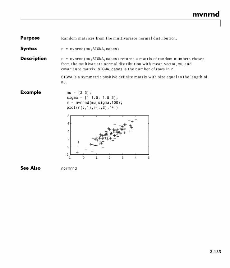
mvnrnd
2mvnrndPurpose Random matrices from the multivariate normal distribution.
Syntax r = mvnrnd(mu,SIGMA,cases)
Description r = mvnrnd(mu,SIGMA,cases) returns a matrix of random numbers chosenfrom the multivariate normal distribution with mean vector, mu, andcovariance matrix, SIGMA. cases is the number of rows in r.
SIGMA is a symmetric positive definite matrix with size equal to the length ofmu.
Example mu = [2 3];sigma = [1 1.5; 1.5 3];r = mvnrnd(mu,sigma,100);plot(r(:,1),r(:,2),'+')
See Also normrnd
-1 0 1 2 3 4 5-2
0
2
4
6
8
2-135
nanmax
2nanmaxPurpose Maximum ignoring NaNs.
Syntax m = nanmax(a)
[m,ndx] = nanmax(a)
m = nanmax(a,b)
Description m = nanmax(a) returns the maximum with NaNs treated as missing. Forvectors, nanmax(a) is the largest non-NaN element in a. For matrices,nanmax(A) is a row vector containing the maximum non-NaN element from eachcolumn.
[m,ndx] = nanmax(a) also returns the indices of the maximum values in vectorndx.
m = nanmax(a,b) returns the larger of a or b, which must match in size.
Example m = magic(3);m([1 6 8]) = [NaN NaN NaN]
m =
NaN 1 6 3 5 NaN 4 NaN 2
[nmax,maxidx] = nanmax(m)
nmax =
4 5 6
maxidx =
3 2 1
See Also nanmin, nanmean, nanmedian, nanstd, nansum
2-136
nanmean
2nanmeanPurpose Mean ignoring NaNs
Syntax y = nanmean(X)
Description nanmean(X) the average treating NaNs as missing values.
For vectors, nanmean(x) is the mean of the non-NaN elements of x. For matrices,nanmean(X) is a row vector containing the mean of the non-NaN elements ineach column.
Example m = magic(3);m([1 6 8]) = [NaN NaN NaN]
m =
NaN 1 6 3 5 NaN 4 NaN 2
nmean = nanmean(m)
nmean =
3.5000 3.0000 4.0000
See Also nanmin, nanmax, nanmedian, nanstd, nansum
2-137

nanmedian
2nanmedianPurpose Median ignoring NaNs
Syntax y = nanmedian(X)
Description nanmedian(X) the median treating NaNs as missing values.
For vectors, nanmedian(x) is the median of the non-NaN elements of x. Formatrices, nanmedian(X) is a row vector containing the median of the non-NaNelements in each column of X.
Example m = magic(4);m([1 6 9 11]) = [NaN NaN NaN NaN]
m =
NaN 2 NaN 13 5 NaN 10 8 9 7 NaN 12 4 14 15 1
nmedian = nanmedian(m)
nmedian =
5.0000 7.0000 12.5000 10.0000
See Also nanmin, nanmax, nanmean, nanstd, nansum
2-138
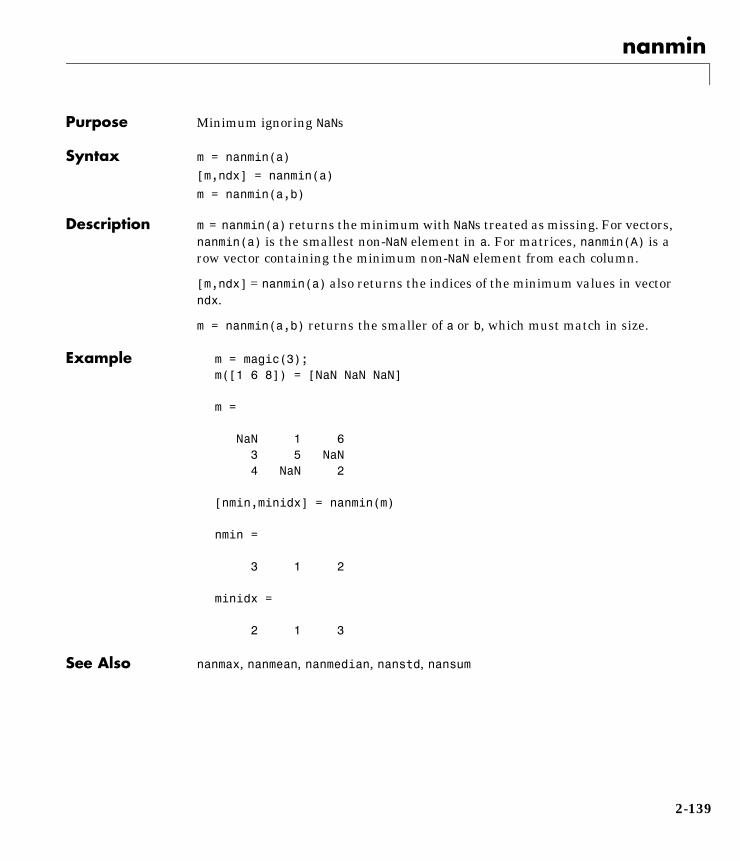
nanmin
2nanminPurpose Minimum ignoring NaNs
Syntax m = nanmin(a)
[m,ndx] = nanmin(a)
m = nanmin(a,b)
Description m = nanmin(a) returns the minimum with NaNs treated as missing. For vectors,nanmin(a) is the smallest non-NaN element in a. For matrices, nanmin(A) is arow vector containing the minimum non-NaN element from each column.
[m,ndx] = nanmin(a) also returns the indices of the minimum values in vectorndx.
m = nanmin(a,b) returns the smaller of a or b, which must match in size.
Example m = magic(3);m([1 6 8]) = [NaN NaN NaN]
m =
NaN 1 6 3 5 NaN 4 NaN 2
[nmin,minidx] = nanmin(m)
nmin =
3 1 2
minidx =
2 1 3
See Also nanmax, nanmean, nanmedian, nanstd, nansum
2-139
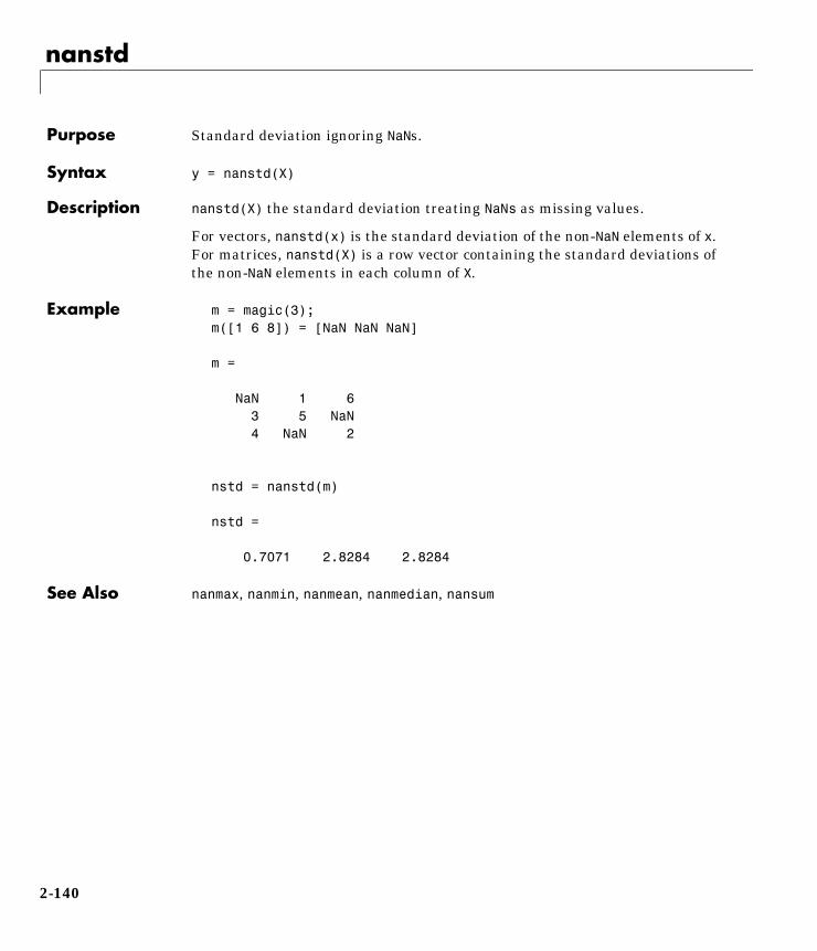
nanstd
2nanstdPurpose Standard deviation ignoring NaNs.
Syntax y = nanstd(X)
Description nanstd(X) the standard deviation treating NaNs as missing values.
For vectors, nanstd(x) is the standard deviation of the non-NaN elements of x.For matrices, nanstd(X) is a row vector containing the standard deviations ofthe non-NaN elements in each column of X.
Example m = magic(3);m([1 6 8]) = [NaN NaN NaN]
m =
NaN 1 6 3 5 NaN 4 NaN 2
nstd = nanstd(m)
nstd =
0.7071 2.8284 2.8284
See Also nanmax, nanmin, nanmean, nanmedian, nansum
2-140
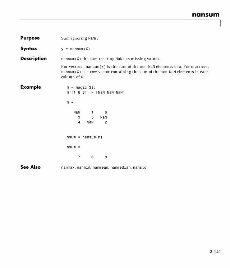
nansum
2nansumPurpose Sum ignoring NaNs.
Syntax y = nansum(X)
Description nansum(X) the sum treating NaNs as missing values.
For vectors, nansum(x) is the sum of the non-NaN elements of x. For matrices,nansum(X) is a row vector containing the sum of the non-NaN elements in eachcolumn of X.
Example m = magic(3);m([1 6 8]) = [NaN NaN NaN]
m =
NaN 1 6 3 5 NaN 4 NaN 2
nsum = nansum(m)
nsum =
7 6 8
See Also nanmax, nanmin, nanmean, nanmedian, nanstd
2-141
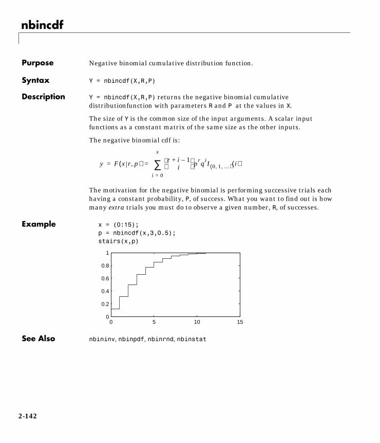
nbincdf
2nbincdfPurpose Negative binomial cumulative distribution function.
Syntax Y = nbincdf(X,R,P)
Description Y = nbincdf(X,R,P) returns the negative binomial cumulativedistributionfunction with parameters R and P at the values in X.
The size of Y is the common size of the input arguments. A scalar inputfunctions as a constant matrix of the same size as the other inputs.
The negative binomial cdf is:
The motivation for the negative binomial is performing successive trials eachhaving a constant probability, P, of success. What you want to find out is howmany extra trials you must do to observe a given number, R, of successes.
Example x = (0:15);p = nbincdf(x,3,0.5);stairs(x,p)
See Also nbininv, nbinpdf, nbinrnd, nbinstat
y F x r p,( ) r i 1–+i
i 0=
x
∑ prqiI 0 1 …, ,( ) i( )= =
0 5 10 150
0.2
0.4
0.6
0.8
1
2-142
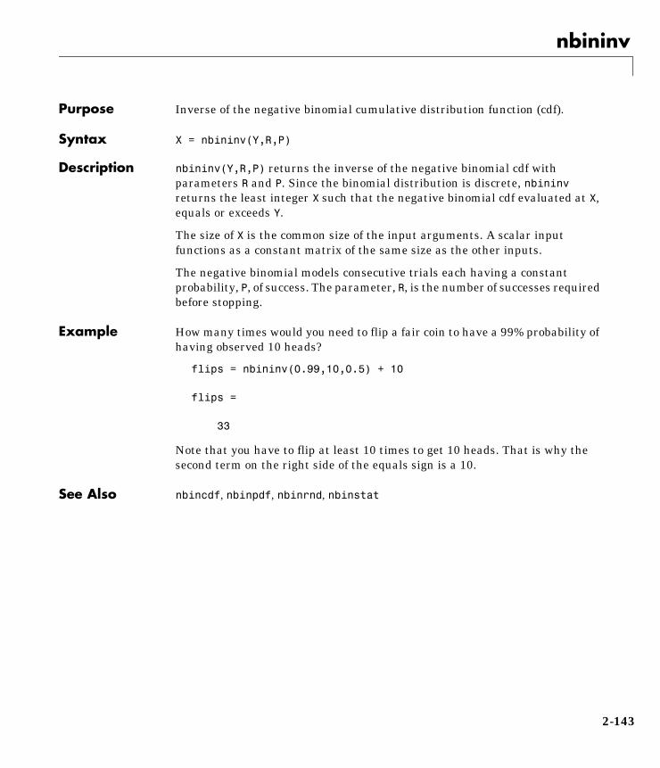
nbininv
2nbininvPurpose Inverse of the negative binomial cumulative distribution function (cdf).
Syntax X = nbininv(Y,R,P)
Description nbininv(Y,R,P) returns the inverse of the negative binomial cdf withparameters R and P. Since the binomial distribution is discrete, nbininvreturns the least integer X such that the negative binomial cdf evaluated at X,equals or exceeds Y.
The size of X is the common size of the input arguments. A scalar inputfunctions as a constant matrix of the same size as the other inputs.
The negative binomial models consecutive trials each having a constantprobability, P, of success. The parameter, R, is the number of successes requiredbefore stopping.
Example How many times would you need to flip a fair coin to have a 99% probability ofhaving observed 10 heads?
flips = nbininv(0.99,10,0.5) + 10
flips =
33
Note that you have to flip at least 10 times to get 10 heads. That is why thesecond term on the right side of the equals sign is a 10.
See Also nbincdf, nbinpdf, nbinrnd, nbinstat
2-143
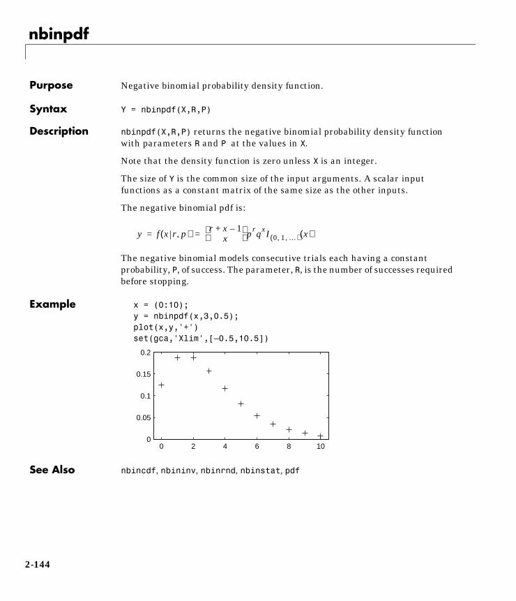
nbinpdf
2nbinpdfPurpose Negative binomial probability density function.
Syntax Y = nbinpdf(X,R,P)
Description nbinpdf(X,R,P) returns the negative binomial probability density functionwith parameters R and P at the values in X.
Note that the density function is zero unless X is an integer.
The size of Y is the common size of the input arguments. A scalar inputfunctions as a constant matrix of the same size as the other inputs.
The negative binomial pdf is:
The negative binomial models consecutive trials each having a constantprobability, P, of success. The parameter, R, is the number of successes requiredbefore stopping.
Example x = (0:10);y = nbinpdf(x,3,0.5);plot(x,y,'+')set(gca,'Xlim',[–0.5,10.5])
See Also nbincdf, nbininv, nbinrnd, nbinstat, pdf
y f x r p,( ) r x 1–+x
prqxI 0 1 …, ,( ) x( )= =
0 2 4 6 8 100
0.05
0.1
0.15
0.2
2-144
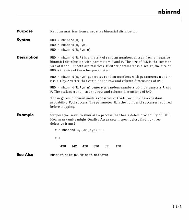
nbinrnd
2nbinrndPurpose Random matrices from a negative binomial distribution.
Syntax RND = nbinrnd(R,P)
RND = nbinrnd(R,P,m)
RND = nbinrnd(R,P,m,n)
Description RND = nbinrnd(R,P) is a matrix of random numbers chosen from a negativebinomial distribution with parameters R and P. The size of RND is the commonsize of R and P if both are matrices. If either parameter is a scalar, the size ofRND is the size of the other parameter.
RND = nbinrnd(R,P,m) generates random numbers with parameters R and P.m is a 1-by-2 vector that contains the row and column dimensions of RND.
RND = nbinrnd(R,P,m,n) generates random numbers with parameters R andP. The scalars m and n are the row and column dimensions of RND.
The negative binomial models consecutive trials each having a constantprobability, P, of success. The parameter, R, is the number of successes requiredbefore stopping.
Example Suppose you want to simulate a process that has a defect probability of 0.01.How many units might Quality Assurance inspect before finding threedefective items?
r = nbinrnd(3,0.01,1,6) + 3
r =
496 142 420 396 851 178
See Also nbincdf, nbininv, nbinpdf, nbinstat
2-145

nbinstat
2nbinstatPurpose Mean and variance of the negative binomial distribution.
Syntax [M,V] = nbinstat(R,P)
Description [M,V] = nbinstat(R,P) returns the mean and variance of the negativebinomial distibution with parameters R and P.
For the negative binomial distribution:
• The mean is
• The variance is
where q = 1 – p.
Example p = 0.1:0.2:0.9;r = 1:5;[R,P] = meshgrid(r,p);[M,V] = nbinstat(R,P)
M =
9.0000 18.0000 27.0000 36.0000 45.0000 2.3333 4.6667 7.0000 9.3333 11.6667 1.0000 2.0000 3.0000 4.0000 5.0000 0.4286 0.8571 1.2857 1.7143 2.1429 0.1111 0.2222 0.3333 0.4444 0.5556
V =
90.0000 180.0000 270.0000 360.0000 450.0000 7.7778 15.5556 23.3333 31.1111 38.8889 2.0000 4.0000 6.0000 8.0000 10.0000 0.6122 1.2245 1.8367 2.4490 3.0612 0.1235 0.2469 0.3704 0.4938 0.6173
See Also nbincdf, nbininv, nbinpdf, nbinrnd
rqp------
rq
p2------
2-146
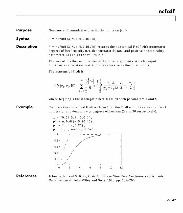
ncfcdf
2ncfcdfPurpose Noncentral F cumulative distribution function (cdf).
Syntax P = ncfcdf(X,NU1,NU2,DELTA)
Description P = ncfcdf(X,NU1,NU2,DELTA) returns the noncentral F cdf with numeratordegrees of freedom (df), NU1, denominator df, NU2, and positive noncentralityparameter, DELTA, at the values in X.
The size of P is the common size of the input arguments. A scalar inputfunctions as a constant matrix of the same size as the other inputs.
The noncentral F cdf is:
where I(x|a,b) is the incomplete beta function with parameters a and b.
Example Compare the noncentral F cdf with δ = 10 to the F cdf with the same number ofnumerator and denominator degrees of freedom (5 and 20 respectively).
x = (0.01:0.1:10.01)';p1 = ncfcdf(x,5,20,10);p = fcdf(x,5,20);plot(x,p,'– –',x,p1,'–')
References Johnson, N., and S. Kotz, Distributions in Statistics: Continuous UnivariateDistributions-2, John Wiley and Sons, 1970. pp. 189–200.
F x ν1 ν2 δ, ,( )
12---δ
j
j!-------------e
δ2---–
Iν1 x⋅
ν2 ν+ 1 x⋅-------------------------ν12------ j+
ν22------,
j 0=
∞
∑=
0 2 4 6 8 10 120
0.2
0.4
0.6
0.8
1
2-147
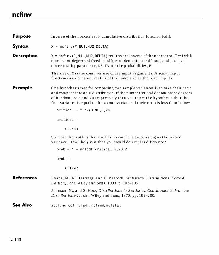
ncfinv
2ncfinvPurpose Inverse of the noncentral F cumulative distribution function (cdf).
Syntax X = ncfinv(P,NU1,NU2,DELTA)
Description X = ncfinv(P,NU1,NU2,DELTA) returns the inverse of the noncentral F cdf withnumerator degrees of freedom (df), NU1, denominator df, NU2, and positivenoncentrality parameter, DELTA, for the probabilities, P.
The size of X is the common size of the input arguments. A scalar inputfunctions as a constant matrix of the same size as the other inputs.
Example One hypothesis test for comparing two sample variances is to take their ratioand compare it to an F distribution. If the numerator and denominator degreesof freedom are 5 and 20 respectively then you reject the hypothesis that thefirst variance is equal to the second variance if their ratio is less than below:
critical = finv(0.95,5,20)
critical =
2.7109
Suppose the truth is that the first variance is twice as big as the secondvariance. How likely is it that you would detect this difference?
prob = 1 – ncfcdf(critical,5,20,2)
prob =
0.1297
References Evans, M., N. Hastings, and B. Peacock, Statistical Distributions, SecondEdition, John Wiley and Sons, 1993. p. 102–105.
Johnson, N., and S. Kotz, Distributions in Statistics: Continuous UnivariateDistributions-2, John Wiley and Sons, 1970. pp. 189–200.
See Also icdf, ncfcdf, ncfpdf, ncfrnd, ncfstat
2-148
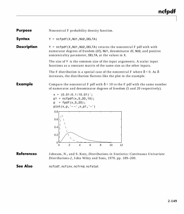
ncfpdf
2ncfpdfPurpose Noncentral F probability density function.
Syntax Y = ncfpdf(X,NU1,NU2,DELTA)
Description Y = ncfpdf(X,NU1,NU2,DELTA) returns the noncentral F pdf with withnumerator degrees of freedom (df), NU1, denominator df, NU2, and positivenoncentrality parameter, DELTA, at the values in X.
The size of Y is the common size of the input arguments. A scalar inputfunctions as a constant matrix of the same size as the other inputs.
The F distribution is a special case of the noncentral F where δ = 0. As δincreases, the distribution flattens like the plot in the example.
Example Compare the noncentral F pdf with δ = 10 to the F pdf with the same numberof numerator and denominator degrees of freedom (5 and 20 respectively).
x = (0.01:0.1:10.01)';p1 = ncfpdf(x,5,20,10);p = fpdf(x,5,20);plot(x,p,'– –',x,p1,'–')
References Johnson, N., and S. Kotz, Distributions in Statistics: Continuous UnivariateDistributions-2, John Wiley and Sons, 1970. pp. 189–200.
See Also ncfcdf, ncfinv, ncfrnd, ncfstat
0 2 4 6 8 10 120
0.2
0.4
0.6
0.8
2-149

ncfrnd
2ncfrndPurpose Random matrices from the noncentral F distribution.
Syntax R = ncfrnd(NU1,NU2,DELTA)
R = ncfrnd(NU1,NU2,DELTA,m)
R = ncfrnd(NU1,NU2,DELTA,m,n)
Description R = ncfrnd(NU1,NU2,DELTA) returns a matrix of random numbers chosen fromthe noncentral F distribution with parameters NU1, NU2 and DELTA. The size ofR is the common size of NU1, NU2 and DELTA if all are matrices. If any parameteris a scalar, the size of R is the size of the other parameters.
R = ncfrnd(NU1,NU2,DELTA,m) returns a matrix of random numbers withparameters NU1, NU2 and DELTA. m is a 1-by-2 vector that contains the row andcolumn dimensions of R.
R = ncfrnd(NU1,NU2,DELTA,m,n) generates random numbers withparameters NU1, NU2 and DELTA. The scalars m and n are the row and columndimensions of R.
Example Compute 6 random numbers from a noncentral F distribution with 10numerator degrees of freedom, 100 denominator degrees of freedom and anoncentrality parameter, δ, of 4.0. Compare this to the F distribution with thesame degrees of freedom.
r = ncfrnd(10,100,4,1,6)r =
2.5995 0.8824 0.8220 1.4485 1.4415 1.4864
r1 = frnd(10,100,1,6)r1 =
0.9826 0.5911 1.0967 0.9681 2.0096 0.6598
References Johnson, N., and S. Kotz, Distributions in Statistics: Continuous UnivariateDistributions-2, John Wiley and Sons, 1970. pp. 189–200.
See Also ncfcdf, ncfinv, ncfpdf, ncfstat
2-150
ncfstat
2ncfstatPurpose Mean and variance of the noncentral F distribution.
Syntax [M,V] = ncfstat(NU1,NU2,DELTA)
Description [M,V] = ncfstat(NU1,NU2,DELTA) returns the mean and variance of thenoncentral F pdf with NU1 and NU2 degrees of freedom and noncentralityparameter, DELTA.
• The mean is
where ν2 > 2.
• The variance is
where ν2 > 4.
Example [m,v]= ncfstat(10,100,4)
m =
1.4286
v =
3.9200
References Evans, M., N. Hastings, and B. Peacock, Statistical Distributions, SecondEdition, John Wiley and Sons, 1993. p. 73–74.
Johnson, N., and S. Kotz, Distributions in Statistics: Continuous UnivariateDistributions-2, John Wiley and Sons, 1970. pp. 189–200.
See Also ncfcdf, ncfinv, ncfpdf, ncfrnd
ν2 δ ν+ 1( )ν1 ν2 2–( )--------------------------
2ν2ν1------
2 δ ν+ 1( )2 2δ ν+ 1( ) ν2 2–( )+
ν2 2–( )2 ν2 4–( )--------------------------------------------------------------------------
2-151
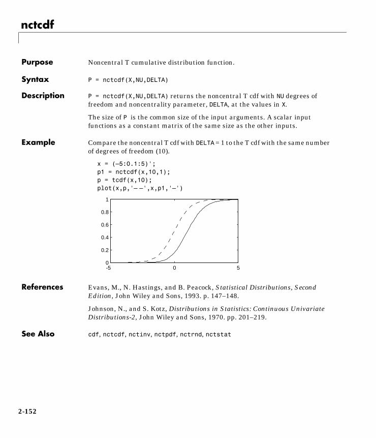
nctcdf
2nctcdfPurpose Noncentral T cumulative distribution function.
Syntax P = nctcdf(X,NU,DELTA)
Description P = nctcdf(X,NU,DELTA) returns the noncentral T cdf with NU degrees offreedom and noncentrality parameter, DELTA, at the values in X.
The size of P is the common size of the input arguments. A scalar inputfunctions as a constant matrix of the same size as the other inputs.
Example Compare the noncentral T cdf with DELTA = 1 to the T cdf with the same numberof degrees of freedom (10).
x = (–5:0.1:5)';p1 = nctcdf(x,10,1);p = tcdf(x,10);plot(x,p,'– –',x,p1,'–')
References Evans, M., N. Hastings, and B. Peacock, Statistical Distributions, SecondEdition, John Wiley and Sons, 1993. p. 147–148.
Johnson, N., and S. Kotz, Distributions in Statistics: Continuous UnivariateDistributions-2, John Wiley and Sons, 1970. pp. 201–219.
See Also cdf, nctcdf, nctinv, nctpdf, nctrnd, nctstat
-5 0 50
0.2
0.4
0.6
0.8
1
2-152
nctinv
2nctinvPurpose Inverse of the noncentral T cumulative distribution.
Syntax X = nctinv(P,NU,DELTA)
Description X = nctinv(P,NU,DELTA) returns the inverse of the noncentral T cdf with NUdegrees of freedom and noncentrality parameter, DELTA, for the probabilities, P.
The size of X is the common size of the input arguments. A scalar inputfunctions as a constant matrix of the same size as the other inputs.
Example x = nctinv([.1 .2],10,1)
x =
–0.2914 0.1618
References Evans, M., N. Hastings, and B. Peacock, Statistical Distributions, SecondEdition, John Wiley and Sons, 1993. p. 147–148.
Johnson, N., and S. Kotz, Distributions in Statistics: Continuous UnivariateDistributions-2, John Wiley and Sons, 1970. pp. 201–219.
See Also icdf, nctcdf, nctpdf, nctrnd, nctstat
2-153

nctpdf
2nctpdfPurpose Noncentral T probability density function (pdf).
Syntax Y = nctpdf(X,V,DELTA)
Description Y = nctpdf(X,V,DELTA) returns the noncentral T pdf with V degrees of freedomand noncentrality parameter, DELTA, at the values in X.
The size of Y is the common size of the input arguments. A scalar inputfunctions as a constant matrix of the same size as the other inputs.
Example Compare the noncentral T pdf with DELTA = 1 to the T pdf with the samenumber of degrees of freedom (10).
x = (–5:0.1:5)';p1 = nctpdf(x,10,1);p = tpdf(x,10);plot(x,p,'– –',x,p1,'–')
References Evans, M., N. Hastings, and B. Peacock, Statistical Distributions, SecondEdition, John Wiley and Sons, 1993. p. 147–148.
Johnson, N., and S. Kotz, Distributions in Statistics: Continuous UnivariateDistributions-2, John Wiley and Sons, 1970. pp. 201–219.
See Also nctcdf, nctinv, nctrnd, nctstat, pdf
-5 0 50
0.1
0.2
0.3
0.4
2-154
nctrnd
2nctrndPurpose Random matrices from noncentral T distribution.
Syntax R = nctrnd(V,DELTA)
R = nctrnd(V,DELTA,m)
R = nctrnd(V,DELTA,m,n)
Description R = nctrnd(V,DELTA) returns a matrix of random numbers chosen from thenoncentral T distribution with parameters V and DELTA. The size of R is thecommon size of V and DELTA if both are matrices. If either parameter is a scalar,the size of R is the size of the other parameter.
R = nctrnd(V,DELTA,m) returns a matrix of random numbers with parametersV and DELTA. m is a 1-by-2 vector that contains the row and column dimensionsof R.
R = nctrnd(V,DELTA,m,n) generates random numbers with parameters V andDELTA. The scalars m and n are the row and column dimensions of R.
Example nctrnd(10,1,5,1)
ans =
1.6576 1.0617 1.4491 0.2930 3.6297
References Evans, M., N. Hastings, and B. Peacock, Statistical Distributions, SecondEdition, John Wiley and Sons, 1993. p. 147–148.
Johnson, N., and S. Kotz, Distributions in Statistics: Continuous UnivariateDistributions-2, John Wiley and Sons, 1970. pp. 201–219.
See Also nctcdf, nctinv, nctpdf, nctstat
2-155
nctstat
2nctstatPurpose Mean and variance for the noncentral t distribution.
Syntax [M,V] = nctstat(NU,DELTA)
Description [M,V] = nctstat(NU,DELTA) returns the mean and variance of the noncentralt pdf with NU degrees of freedom and noncentrality parameter, DELTA.
• The mean is
where ν > 1.
• The variance is
where ν > 2.
Example [m,v] = nctstat(10,1)
m =
1.0837
v =
1.3255
References Evans, M., N. Hastings, and B. Peacock, Statistical Distributions, SecondEdition, John Wiley and Sons, 1993. p. 147–148.
Johnson, N., and S. Kotz, Distributions in Statistics: Continuous UnivariateDistributions-2, John Wiley and Sons, 1970. pp. 201–219.
See Also nctcdf, nctinv, nctpdf, nctrnd
δ ν 2⁄( )1 2⁄ Γ ν 1–( ) 2⁄( )Γ ν 2⁄( )-------------------------------------------------------------
νν 2–( )----------------- 1 δ2
+( ) ν2---– δ2 Γ ν 1–( ) 2⁄( )
Γ ν 2⁄( )---------------------------------2
2-156
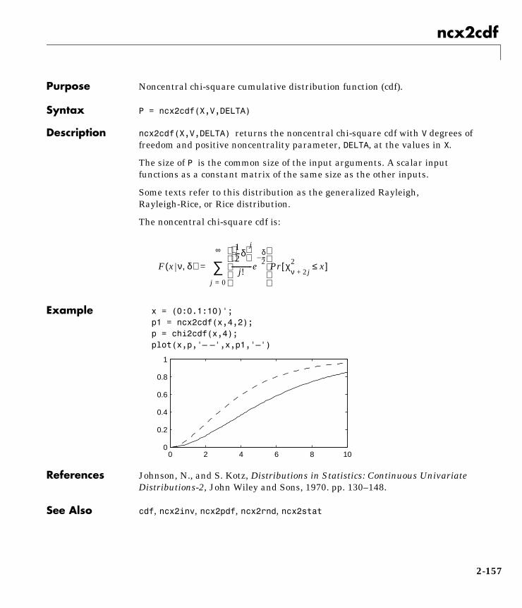
ncx2cdf
2ncx2cdfPurpose Noncentral chi-square cumulative distribution function (cdf).
Syntax P = ncx2cdf(X,V,DELTA)
Description ncx2cdf(X,V,DELTA) returns the noncentral chi-square cdf with V degrees offreedom and positive noncentrality parameter, DELTA, at the values in X.
The size of P is the common size of the input arguments. A scalar inputfunctions as a constant matrix of the same size as the other inputs.
Some texts refer to this distribution as the generalized Rayleigh,Rayleigh-Rice, or Rice distribution.
The noncentral chi-square cdf is:
Example x = (0:0.1:10)';p1 = ncx2cdf(x,4,2);p = chi2cdf(x,4);plot(x,p,'– –',x,p1,'–')
References Johnson, N., and S. Kotz, Distributions in Statistics: Continuous UnivariateDistributions-2, John Wiley and Sons, 1970. pp. 130–148.
See Also cdf, ncx2inv, ncx2pdf, ncx2rnd, ncx2stat
F x ν δ,( )
12---δ
j
j!-------------e
δ2---–
Pr χν 2j+
2 x≤[ ]
j 0=
∞
∑=
0 2 4 6 8 100
0.2
0.4
0.6
0.8
1
2-157
ncx2inv
2ncx2invPurpose Inverse of the noncentral chi-square cdf.
Syntax X = ncx2inv(P,V,DELTA)
Description X = ncx2inv(P,V,DELTA) returns the inverse of the noncentral chi-square cdfwith parameters V and DELTA, at the probabilities in P.
The size of X is the common size of the input arguments. A scalar inputfunctions as a constant matrix of the same size as the other inputs.
Algorithm ncx2inv uses Newton's method to converge to the solution.
Example ncx2inv([0.01 0.05 0.1],4,2)
ans =
0.4858 1.1498 1.7066
References Evans, M., N. Hastings, and B. Peacock, Statistical Distributions, SecondEdition, John Wiley and Sons, 1993. p. 50–52.
Johnson, N., and S. Kotz, Distributions in Statistics: Continuous UnivariateDistributions-2, John Wiley and Sons, 1970. pp. 130–148.
See Also ncx2cdf, ncx2pdf, ncx2rnd, ncx2stat
2-158
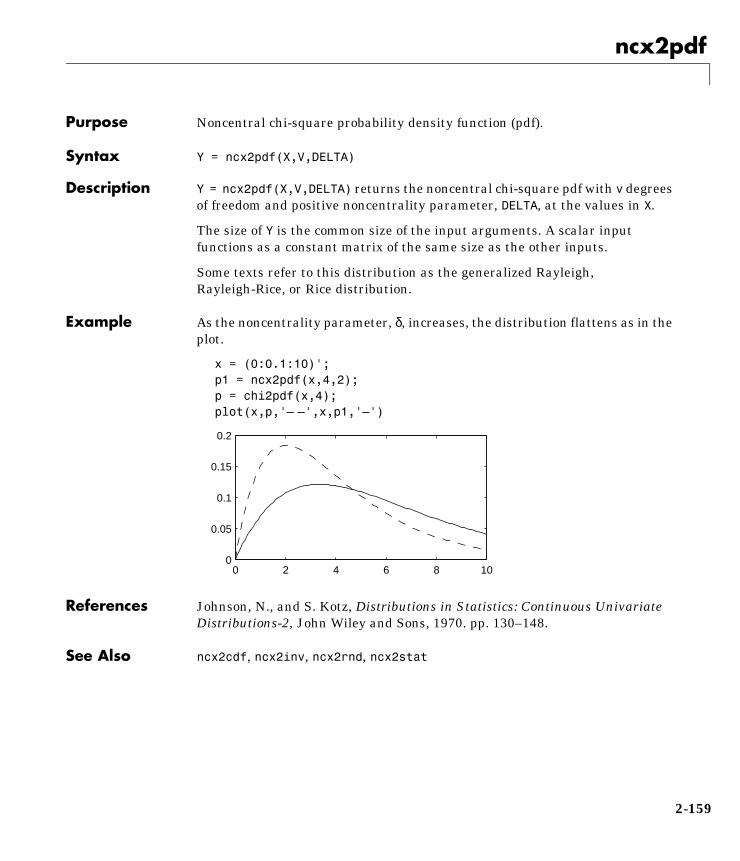
ncx2pdf
2ncx2pdfPurpose Noncentral chi-square probability density function (pdf).
Syntax Y = ncx2pdf(X,V,DELTA)
Description Y = ncx2pdf(X,V,DELTA) returns the noncentral chi-square pdf with v degreesof freedom and positive noncentrality parameter, DELTA, at the values in X.
The size of Y is the common size of the input arguments. A scalar inputfunctions as a constant matrix of the same size as the other inputs.
Some texts refer to this distribution as the generalized Rayleigh,Rayleigh-Rice, or Rice distribution.
Example As the noncentrality parameter, δ, increases, the distribution flattens as in theplot.
x = (0:0.1:10)';p1 = ncx2pdf(x,4,2);p = chi2pdf(x,4);plot(x,p,'– –',x,p1,'–')
References Johnson, N., and S. Kotz, Distributions in Statistics: Continuous UnivariateDistributions-2, John Wiley and Sons, 1970. pp. 130–148.
See Also ncx2cdf, ncx2inv, ncx2rnd, ncx2stat
0 2 4 6 8 100
0.05
0.1
0.15
0.2
2-159

ncx2rnd
2ncx2rndPurpose Random matrices from the noncentral chi-square distribution.
Syntax R = ncx2rnd(V,DELTA)
R = ncx2rnd(V,DELTA,m)
R = ncx2rnd(V,DELTA,m,n)
Description R = ncx2rnd(V,DELTA) returns a matrix of random numbers chosen from thenon-central chisquare distribution with parameters V and DELTA. The size of Ris the common size of V and DELTA if both are matrices. If either parameter is ascalar, the size of R is the size of the other parameter.
R = ncx2rnd(V,DELTA,m) returns a matrix of random numbers withparameters V and DELTA. m is a 1-by-2 vector that contains the row and columndimensions of R.
R = ncx2rnd(V,DELTA,m,n) generates random numbers with parameters V andDELTA. The scalars m and n are the row and column dimensions of R.
Example ncx2rnd(4,2,6,3)
ans =
6.8552 5.9650 11.2961 5.2631 4.2640 5.9495 9.1939 6.7162 3.8315 10.3100 4.4828 7.1653 2.1142 1.9826 4.6400 3.8852 5.3999 0.9282
References Evans, M., N. Hastings, and B. Peacock, Statistical Distributions, SecondEdition, John Wiley and Sons, 1993. p. 50–52.
Johnson, N., and S. Kotz, Distributions in Statistics: Continuous UnivariateDistributions-2, John Wiley and Sons, 1970. pp. 130–148.
See Also ncx2cdf, ncx2inv, ncx2pdf, ncx2stat
2-160
ncx2stat
2ncx2statPurpose Mean and variance for the noncentral chi-square distribution.
Syntax [M,V] = ncx2stat(NU,DELTA)
Description [M,V] = ncx2stat(NU,DELTA) returns the mean and variance of the noncentralchi-square pdf with NU degrees of freedom and noncentrality parameter, DELTA.
For the noncentral chi-square distribution:
• The mean is .
• The variance is .
Example [m,v] = ncx2stat(4,2)
m =
6
v =
16
References Evans, M., N. Hastings, and B. Peacock, Statistical Distributions, SecondEdition, John Wiley and Sons, 1993. p. 50–52.
Johnson, N., and S. Kotz, Distributions in Statistics: Continuous UnivariateDistributions-2, John Wiley and Sons, 1970. pp. 130–148.
See Also ncx2cdf, ncx2inv, ncx2pdf, ncx2rnd
ν δ+
2 ν 2δ+( )
2-161

nlinfit
2nlinfitPurpose Nonlinear least-squares data fitting by the Gauss-Newton method.
Syntax [beta,r,J] = nlinfit(X,y,'model',beta0)
Description beta = nlinfit(X,y,'model',beta0) returns the coefficients of the nonlinearfunction described in 'model'.
'model' is a user-supplied function having the form: . It returns thepredicted values of y given initial parameter estimates, β, and the independentvariable, X.
The matrix, X, has one column per independent variable. The response, y, is acolumn vector with the same number of rows as X.
[beta,r,J] = nlinfit(X,y,'model',beta0) returns the fitted coefficients,beta, the residuals, r, and the Jacobian, J, for use with nlintool to produceerror estimates on predictions.
Example load reactionbetafit = nlinfit(reactants,rate,'hougen',beta)
betafit = 1.2526 0.0628 0.0400 0.1124 1.1914
See Also nlintool
y f β X,( )=
2-162
nlintool
2nlintoolPurpose Fits a nonlinear equation to data and displays an interactive graph.
Syntax nlintool(x,y,'model',beta0)
nlintool(x,y,'model',beta0,alpha)
nlintool(x,y,'model',beta0,alpha,'xname','yname')
Description nlintool(x,y,'model',beta0) is a prediction plot that provides a nonlinearcurve fit to (x,y) data. It plots a 95% global confidence interval for predictionsas two red curves. beta0 is a vector containing initial guesses for theparameters.
nlintool(x,y,'model',beta0,alpha) plots a 100(1 – alpha) percentconfidence interval for predictions.
nlintool displays a “vector” of plots, one for each column of the matrix ofinputs, x. The response variable, y, is a column vector that matches the numberof rows in x.
The default value for alpha is 0.05, which produces 95% confidence intervals.
nlintool(x,y,'model',beta0,alpha,'xname','yname') labels the plot usingthe string matrix, 'xname' for the X variables and the string 'yname' for the Yvariable.
You can drag the dotted white reference line and watch the predicted valuesupdate simultaneously. Alternatively, you can get a specific prediction bytyping the value for X into an editable text field. Use the pop-up menu labeledExport to move specified variables to the base workspace.
Example See the section “Nonlinear Regression Models” in Chapter 1.
See Also nlinfit, rstool
2-163
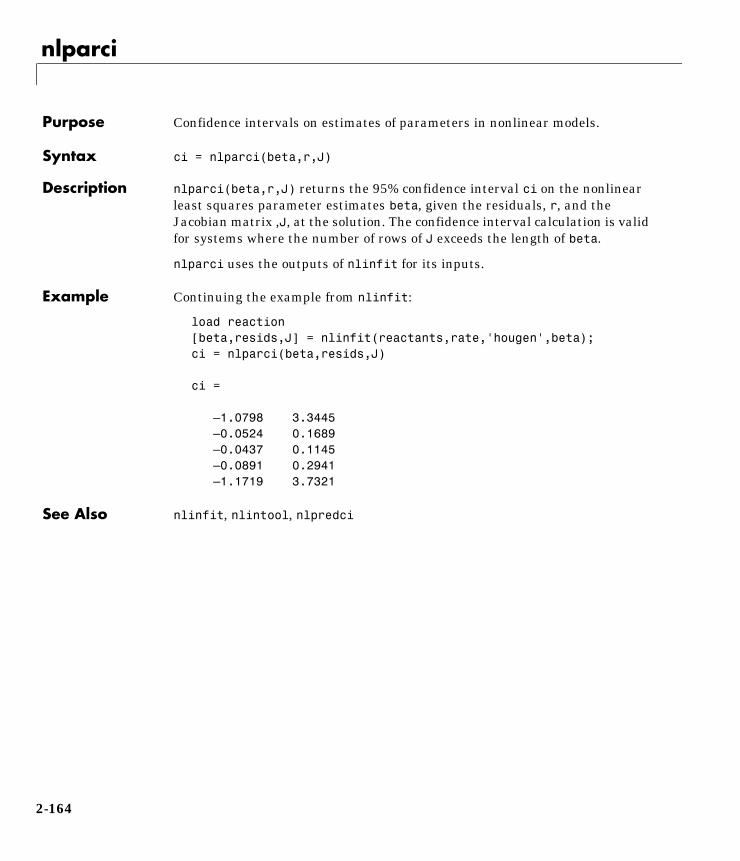
nlparci
2nlparciPurpose Confidence intervals on estimates of parameters in nonlinear models.
Syntax ci = nlparci(beta,r,J)
Description nlparci(beta,r,J) returns the 95% confidence interval ci on the nonlinearleast squares parameter estimates beta, given the residuals, r, and theJacobian matrix ,J, at the solution. The confidence interval calculation is validfor systems where the number of rows of J exceeds the length of beta.
nlparci uses the outputs of nlinfit for its inputs.
Example Continuing the example from nlinfit:
load reaction[beta,resids,J] = nlinfit(reactants,rate,'hougen',beta);ci = nlparci(beta,resids,J)
ci =
–1.0798 3.3445 –0.0524 0.1689 –0.0437 0.1145 –0.0891 0.2941 –1.1719 3.7321
See Also nlinfit, nlintool, nlpredci
2-164
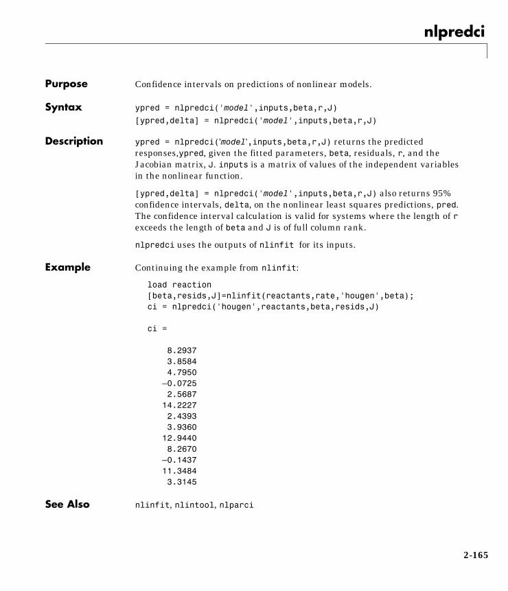
nlpredci
2nlpredciPurpose Confidence intervals on predictions of nonlinear models.
Syntax ypred = nlpredci('model',inputs,beta,r,J)
[ypred,delta] = nlpredci('model',inputs,beta,r,J)
Description ypred = nlpredci('model',inputs,beta,r,J) returns the predictedresponses,ypred, given the fitted parameters, beta, residuals, r, and theJacobian matrix, J. inputs is a matrix of values of the independent variablesin the nonlinear function.
[ypred,delta] = nlpredci('model',inputs,beta,r,J) also returns 95%confidence intervals, delta, on the nonlinear least squares predictions, pred.The confidence interval calculation is valid for systems where the length of rexceeds the length of beta and J is of full column rank.
nlpredci uses the outputs of nlinfit for its inputs.
Example Continuing the example from nlinfit:
load reaction[beta,resids,J]=nlinfit(reactants,rate,'hougen',beta);ci = nlpredci('hougen',reactants,beta,resids,J)
ci =
8.2937 3.8584 4.7950 –0.0725 2.5687 14.2227 2.4393 3.9360 12.9440 8.2670 –0.1437 11.3484 3.3145
See Also nlinfit, nlintool, nlparci
2-165

normcdf
2normcdfPurpose Normal cumulative distribution function (cdf).
Syntax P = normcdf(X,MU,SIGMA)
Description normcdf(X,MU,SIGMA) computes the normal cdf with parameters MU and SIGMAat the values in X. The arguments X, MU and SIGMA must all be the same sizeexcept that scalar arguments function as constant matrices of the common sizeof the other arguments.
The parameter SIGMA must be positive.
The normal cdf is:
The result, p, is the probability that a single observation from a normaldistribution with parameters µ and σ will fall in the interval (–∞ x].
The standard normal distribution has µ = 0 and σ = 1.
Examples What is the probability that an observation from a standard normaldistribution will fall on the interval [–1 1]?
p = normcdf([–1 1]);p(2) – p(1)
ans =
0.6827
More generally, about 68% of the observations from a normal distribution fallwithin one standard deviation,σ, of the mean, µ.
p F x µ σ,( )1
σ 2π--------------- e
t µ–( )– 2
2σ2---------------------
td∞–
x
∫= =
2-166

normfit
2normfitPurpose Parameter estimates and confidence intervals for normal data.
Syntax [muhat,sigmahat,muci,sigmaci] = normfit(X)
[muhat,sigmahat,muci,sigmaci] = normfit(X,alpha)
Description [muhat,sigmahat,muci,sigmaci] = normfit(X) returns estimates, muhat andsigmahat, of the parameters, µ and σ, of the normal distribution given thematrix of data, X. muci and sigmaci are 95% confidence intervals. muci andsigmaci have two rows and as many columns as the data matrix, X. The top rowis the lower bound of the confidence interval and the bottom row is the upperbound.
[muhat,sigmahat,muci,sigmaci] = normfit(X,alpha) gives estimates and100(1–alpha) percent confidence intervals. For example, alpha = 0.01 gives99% confidence intervals.
Example In this example the data is a two-column random normal matrix. Both columnshave µ = 10 and σ = 2. Note that the confidence intervals below contain the“true values.”
r = normrnd(10,2,100,2);[mu,sigma,muci,sigmaci] = normfit(r)
mu = 10.1455 10.0527
sigma = 1.9072 2.1256
muci = 9.7652 9.6288 10.5258 10.4766
sigmaci = 1.6745 1.8663 2.2155 2.4693
See Also betafit, binofit, expfit, gamfit, poissfit, unifit, weibfit
2-167
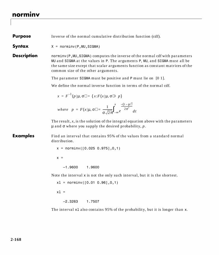
norminv
2norminvPurpose Inverse of the normal cumulative distribution function (cdf).
Syntax X = norminv(P,MU,SIGMA)
Description norminv(P,MU,SIGMA) computes the inverse of the normal cdf with parametersMU and SIGMA at the values in P. The arguments P, MU, and SIGMA must all bethe same size except that scalar arguments function as constant matrices of thecommon size of the other arguments.
The parameter SIGMA must be positive and P must lie on [0 1].
We define the normal inverse function in terms of the normal cdf.
The result, x, is the solution of the integral equation above with the parametersµ and σ where you supply the desired probability, p.
Examples Find an interval that contains 95% of the values from a standard normaldistribution.
x = norminv([0.025 0.975],0,1)
x =
–1.9600 1.9600
Note the interval x is not the only such interval, but it is the shortest.
xl = norminv([0.01 0.96],0,1)
xl =
–2.3263 1.7507
The interval xl also contains 95% of the probability, but it is longer than x.
x F 1– p µ σ,( ) x:F x µ σ,( ) p={ }= =
where p F x µ σ,( )1
σ 2π--------------- e
t µ–( )– 2
2σ2---------------------
td∞–
x
∫= =
2-168
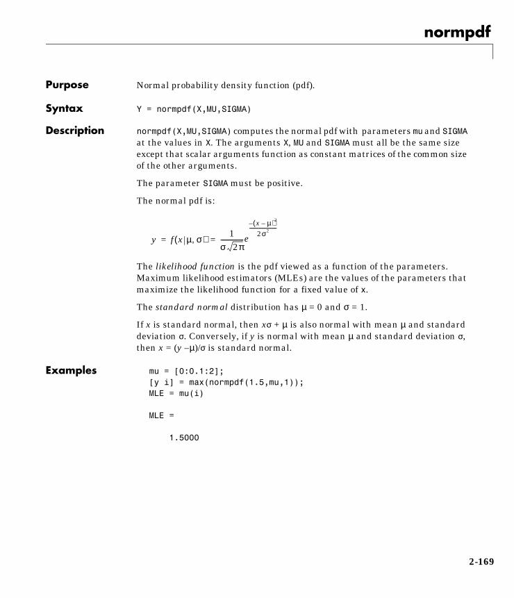
normpdf
2normpdfPurpose Normal probability density function (pdf).
Syntax Y = normpdf(X,MU,SIGMA)
Description normpdf(X,MU,SIGMA) computes the normal pdf with parameters mu and SIGMAat the values in X. The arguments X, MU and SIGMA must all be the same sizeexcept that scalar arguments function as constant matrices of the common sizeof the other arguments.
The parameter SIGMA must be positive.
The normal pdf is:
The likelihood function is the pdf viewed as a function of the parameters.Maximum likelihood estimators (MLEs) are the values of the parameters thatmaximize the likelihood function for a fixed value of x.
The standard normal distribution has µ = 0 and σ = 1.
If x is standard normal, then xσ + µ is also normal with mean µ and standarddeviation σ. Conversely, if y is normal with mean µ and standard deviation σ,then x = (y –µ)/σ is standard normal.
Examples mu = [0:0.1:2];[y i] = max(normpdf(1.5,mu,1));MLE = mu(i)
MLE =
1.5000
y f x µ σ,( )1
σ 2π---------------e
x µ–( )– 2
2σ2----------------------
= =
2-169
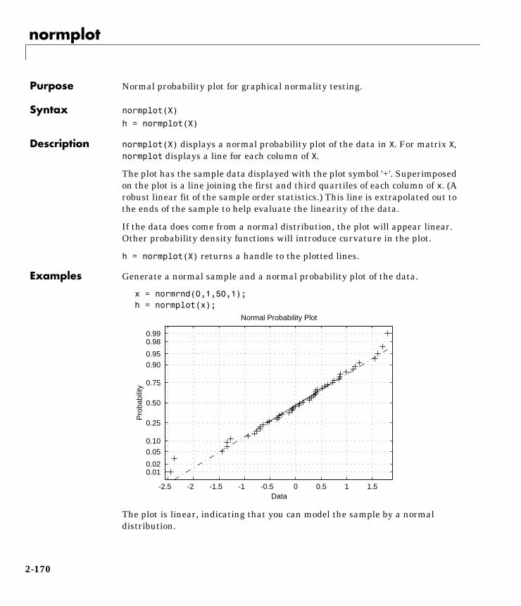
normplot
2normplotPurpose Normal probability plot for graphical normality testing.
Syntax normplot(X)
h = normplot(X)
Description normplot(X) displays a normal probability plot of the data in X. For matrix X,normplot displays a line for each column of X.
The plot has the sample data displayed with the plot symbol '+'. Superimposedon the plot is a line joining the first and third quartiles of each column of x. (Arobust linear fit of the sample order statistics.) This line is extrapolated out tothe ends of the sample to help evaluate the linearity of the data.
If the data does come from a normal distribution, the plot will appear linear.Other probability density functions will introduce curvature in the plot.
h = normplot(X) returns a handle to the plotted lines.
Examples Generate a normal sample and a normal probability plot of the data.
x = normrnd(0,1,50,1);h = normplot(x);
The plot is linear, indicating that you can model the sample by a normaldistribution.
-2.5 -2 -1.5 -1 -0.5 0 0.5 1 1.5
0.01 0.02
0.05
0.10
0.25
0.50
0.75
0.90
0.95
0.98 0.99
Data
Pro
babi
lity
Normal Probability Plot
2-170
normrnd
2normrndPurpose Random numbers from the normal distribution.
Syntax R = normrnd(MU,SIGMA)
R = normrnd(MU,SIGMA,m)
R = normrnd(MU,SIGMA,m,n)
Description R = normrnd(MU,SIGMA) generates normal random numbers with mean, MU,and standard deviation, SIGMA . The size of R is the common size of MU andSIGMA if both are matrices. If either parameter is a scalar, the size of R is thesize of the other parameter.
R = normrnd(MU,SIGMA,m) generates normal random numbers withparameters MU and SIGMA. m is a 1-by-2 vector that contains the row and columndimensions of R.
R = normrnd(MU,SIGMA,m,n) generates normal random numbers withparameters MU and SIGMA. The scalars m and n are the row and columndimensions of R.
Examples n1 = normrnd(1:6,1./(1:6))
n1 =
2.1650 2.3134 3.0250 4.0879 4.8607 6.2827
n2 = normrnd(0,1,[1 5])
n2 =
0.0591 1.7971 0.2641 0.8717 -1.4462
n3 = normrnd([1 2 3;4 5 6],0.1,2,3)
n3 =
0.9299 1.9361 2.9640 4.1246 5.0577 5.9864
2-171
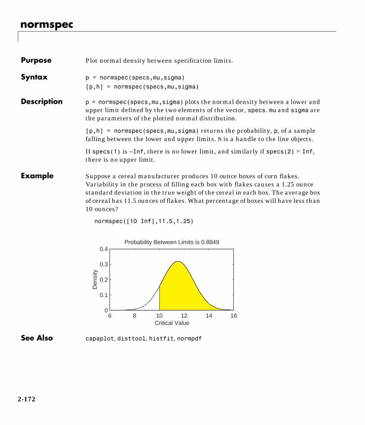
normspec
2normspecPurpose Plot normal density between specification limits.
Syntax p = normspec(specs,mu,sigma)
[p,h] = normspec(specs,mu,sigma)
Description p = normspec(specs,mu,sigma) plots the normal density between a lower andupper limit defined by the two elements of the vector, specs. mu and sigma arethe parameters of the plotted normal distribution.
[p,h] = normspec(specs,mu,sigma) returns the probability, p, of a samplefalling between the lower and upper limits. h is a handle to the line objects.
If specs(1) is –Inf, there is no lower limit, and similarly if specs(2) = Inf,there is no upper limit.
Example Suppose a cereal manufacturer produces 10 ounce boxes of corn flakes.Variability in the process of filling each box with flakes causes a 1.25 ouncestandard deviation in the true weight of the cereal in each box. The average boxof cereal has 11.5 ounces of flakes. What percentage of boxes will have less than10 ounces?
normspec([10 Inf],11.5,1.25)
See Also capaplot, disttool, histfit, normpdf
6 8 10 12 14 160
0.1
0.2
0.3
0.4
Critical Value
Den
sity
Probability Between Limits is 0.8849
2-172

normstat
2normstatPurpose Mean and variance for the normal distribution.
Syntax [M,V] = normstat(MU,SIGMA)
Description For the normal distribution:
• The mean is µ.
• The variance is σ2.
Examples n = 1:5;[m,v] = normstat(n'∗n,n'*n)[m,v] = normstat(n'*n,n'*n)
m =
1 2 3 4 5 2 4 6 8 10 3 6 9 12 15 4 8 12 16 20 5 10 15 20 25
v =
1 4 9 16 25 4 16 36 64 100 9 36 81 144 225 16 64 144 256 400 25 100 225 400 625
2-173
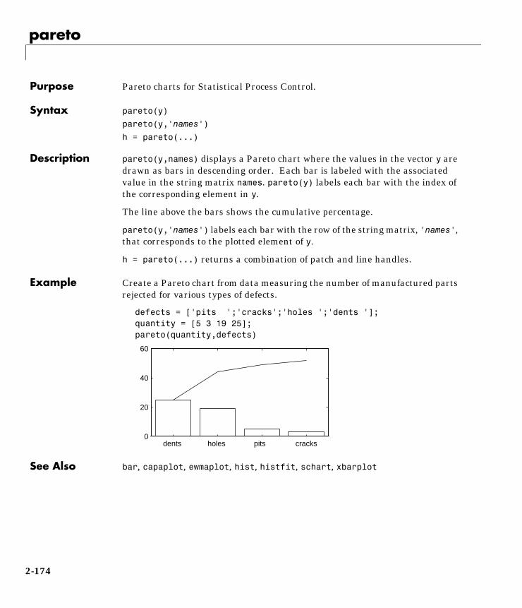
pareto
2paretoPurpose Pareto charts for Statistical Process Control.
Syntax pareto(y)
pareto(y,'names')
h = pareto(...)
Description pareto(y,names) displays a Pareto chart where the values in the vector y aredrawn as bars in descending order. Each bar is labeled with the associatedvalue in the string matrix names. pareto(y) labels each bar with the index ofthe corresponding element in y.
The line above the bars shows the cumulative percentage.
pareto(y,'names') labels each bar with the row of the string matrix, 'names',that corresponds to the plotted element of y.
h = pareto(...) returns a combination of patch and line handles.
Example Create a Pareto chart from data measuring the number of manufactured partsrejected for various types of defects.
defects = ['pits ';'cracks';'holes ';'dents '];quantity = [5 3 19 25];pareto(quantity,defects)
See Also bar, capaplot, ewmaplot, hist, histfit, schart, xbarplot
dents holes pits cracks0
20
40
60
2-174
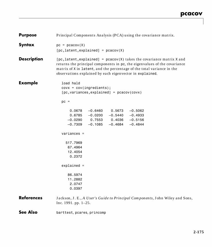
pcacov
2pcacovPurpose Principal Components Analysis (PCA) using the covariance matrix.
Syntax pc = pcacov(X)
[pc,latent,explained] = pcacov(X)
Description [pc,latent,explained] = pcacov(X) takes the covariance matrix X andreturns the principal components in pc, the eigenvalues of the covariancematrix of X in latent, and the percentage of the total variance in theobservations explained by each eigenvector in explained.
Example load haldcovx = cov(ingredients);[pc,variances,explained] = pcacov(covx)
pc =
0.0678 –0.6460 0.5673 –0.5062 0.6785 –0.0200 –0.5440 –0.4933 –0.0290 0.7553 0.4036 –0.5156 –0.7309 –0.1085 –0.4684 –0.4844
variances =
517.7969 67.4964 12.4054 0.2372
explained =
86.5974 11.2882 2.0747 0.0397
References Jackson, J. E., A User's Guide to Principal Components, John Wiley and Sons,Inc. 1991. pp. 1–25.
See Also barttest, pcares, princomp
2-175
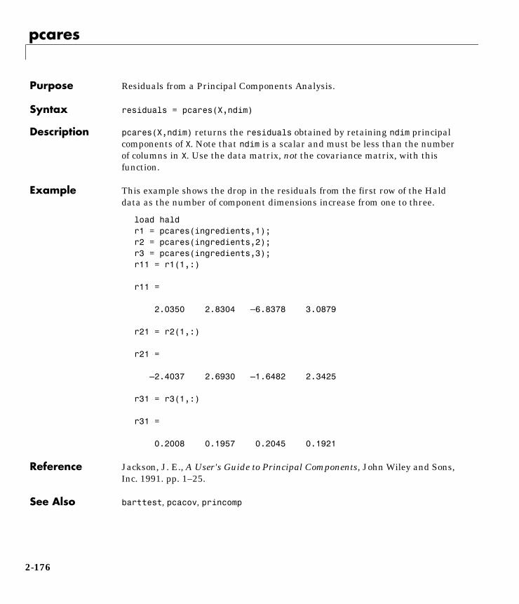
pcares
2pcaresPurpose Residuals from a Principal Components Analysis.
Syntax residuals = pcares(X,ndim)
Description pcares(X,ndim) returns the residuals obtained by retaining ndim principalcomponents of X. Note that ndim is a scalar and must be less than the numberof columns in X. Use the data matrix, not the covariance matrix, with thisfunction.
Example This example shows the drop in the residuals from the first row of the Halddata as the number of component dimensions increase from one to three.
load haldr1 = pcares(ingredients,1);r2 = pcares(ingredients,2);r3 = pcares(ingredients,3);r11 = r1(1,:)
r11 =
2.0350 2.8304 –6.8378 3.0879
r21 = r2(1,:)
r21 =
–2.4037 2.6930 –1.6482 2.3425
r31 = r3(1,:)
r31 =
0.2008 0.1957 0.2045 0.1921
Reference Jackson, J. E., A User's Guide to Principal Components, John Wiley and Sons,Inc. 1991. pp. 1–25.
See Also barttest, pcacov, princomp
2-176
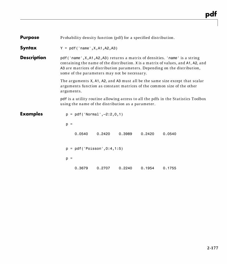
2pdfPurpose Probability density function (pdf) for a specified distribution.
Syntax Y = pdf('name',X,A1,A2,A3)
Description pdf('name',X,A1,A2,A3) returns a matrix of densities. 'name' is a stringcontaining the name of the distribution. X is a matrix of values, and A1, A2, andA3 are matrices of distribution parameters. Depending on the distribution,some of the parameters may not be necessary.
The arguments X, A1, A2, and A3 must all be the same size except that scalararguments function as constant matrices of the common size of the otherarguments.
pdf is a utility routine allowing access to all the pdfs in the Statistics Toolboxusing the name of the distribution as a parameter.
Examples p = pdf('Normal',–2:2,0,1)
p =
0.0540 0.2420 0.3989 0.2420 0.0540
p = pdf('Poisson',0:4,1:5)
p =
0.3679 0.2707 0.2240 0.1954 0.1755
2-177
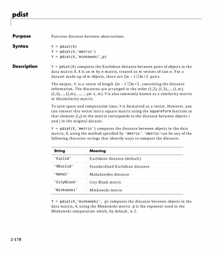
pdist
2pdistPurpose Pairwise distance between observations.
Syntax Y = pdist(X)Y = pdist(X,’metric’)Y = pdist(X,’minkowski’,p)
Description Y = pdist(X) computes the Euclidean distance between pairs of objects in thedata matrix X. X is an m by n matrix, treated as m vectors of size n. For adataset made up of m objects, there are pairs.
The output, Y, is a vector of length , containing the distanceinformation. The distances are arranged in the order (1,2), (1,3),..., (1,m),(2,3),..., (2,m), ..., ...,(m-1, m). Y is also commonly known as a similarity matrixor dissimilarity matrix.
To save space and computation time, Y is formatted as a vector. However, youcan convert this vector into a square matrix using the squareform function sothat element (i,j) in the matrix corresponds to the distance between objects iand j in the original dataset.
Y = pdist(X,'metric') computes the distance between objects in the datamatrix, X, using the method specified by ‘metric’. ‘metric’can be any of thefollowing character strings that identify ways to compute the distance.
Y = pdist(X,’minkowski’, p) computes the distance between objects in thedata matrix, X, using the Minkowski metric. p is the exponent used in theMinkowski computation which, by default, is 2.
String Meaning
‘Euclid’ Euclidean distance (default)
‘SEuclid’ Standardized Euclidean distance
‘Mahal’ Mahalanobis distance
‘CityBlock’ City Block metric
‘Minkowski’ Minkowski metric
m 1–( ) m 2⁄⋅
m 1–( ) m 2⁄⋅
2-178

pdist
Mathematical Definitions of Methods . Given an m-by-n data matrix X, which istreated as m (1-by-n) row vectors x1, x2,..., xm, the various distances betweenthe vector xr and xs are defined as follows:
• Euclidean distance:
• Standardized Euclidean distance:
where D is the diagonal matrix with diagonal elements given by , whichdenotes the variance of the variable Xj over the m objects.
• Mahalanobis distance:
where V is the sample covariance matrix.
• City Block metric:
• Minkowski metric:
Notice that when , it is the City Block case, and when , it is theEuclidean case.
drs2 xr xs–( ) xr xs–( )'=
drs2 xr xs–( )D 1– xr xs–( )'=
vj2
drs2 xr xs–( )'V 1– xr xs–( )=
drs xrj xsj–j 1=
n
∑=
drs xrj xsj–p
j 1=
n
∑
1 p⁄=
p 1= p 2=
2-179
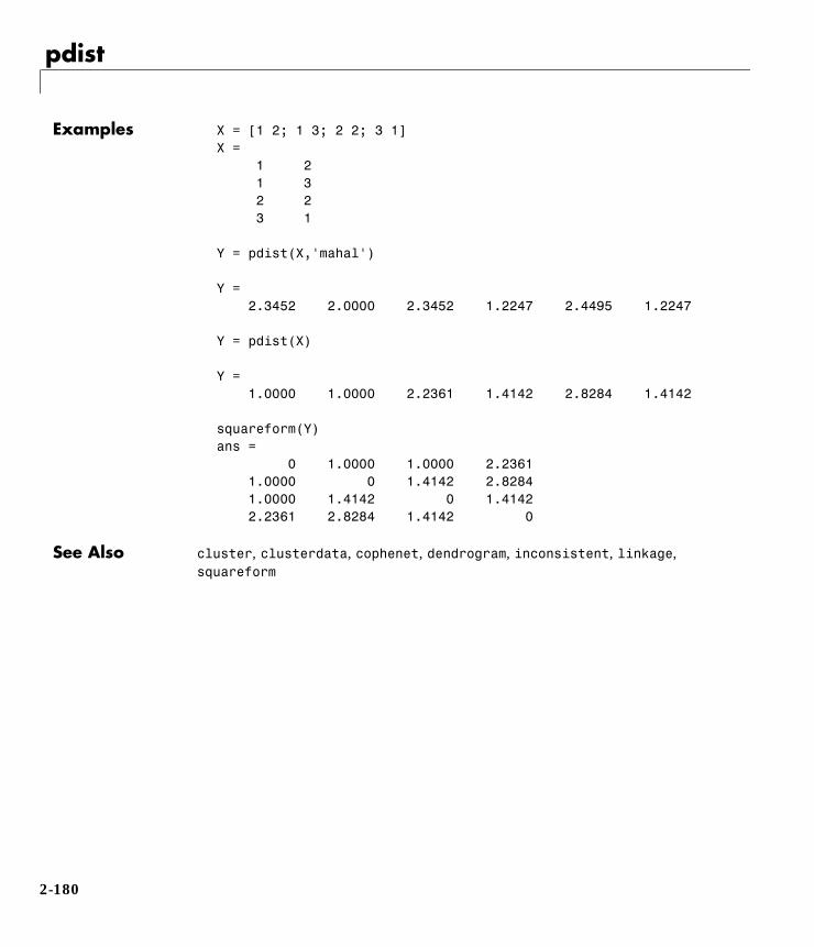
pdist
Examples X = [1 2; 1 3; 2 2; 3 1]X = 1 2 1 3 2 2 3 1
Y = pdist(X,'mahal')
Y = 2.3452 2.0000 2.3452 1.2247 2.4495 1.2247
Y = pdist(X)
Y = 1.0000 1.0000 2.2361 1.4142 2.8284 1.4142
squareform(Y)ans = 0 1.0000 1.0000 2.2361 1.0000 0 1.4142 2.8284 1.0000 1.4142 0 1.4142 2.2361 2.8284 1.4142 0
See Also cluster, clusterdata, cophenet, dendrogram, inconsistent, linkage,squareform
2-180
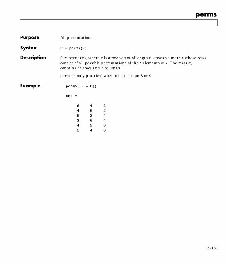
perms
2permsPurpose All permutations.
Syntax P = perms(v)
Description P = perms(v), where v is a row vector of length n, creates a matrix whose rowsconsist of all possible permutations of the n elements of v. The matrix, P,contains n! rows and n columns.
perms is only practical when n is less than 8 or 9.
Example perms([2 4 6])
ans =
6 4 2 4 6 2 6 2 4 2 6 4 4 2 6 2 4 6
2-181

poisscdf
2poisscdfPurpose Poisson cumulative distribution function (cdf).
Syntax P = poisscdf(X,LAMBDA)
Description poisscdf(X,LAMBDA) computes the Poisson cdf with parameter settings LAMBDA at the values in X. The arguments X and LAMBDA must be the same sizeexcept that a scalar argument functions as a constant matrix of the same sizeof the other argument. The parameter, LAMBDA, is positive.
The Poisson cdf is:
Examples For example, consider a Quality Assurance department that performs randomtests of individual hard disks. Their policy is to shut down the manufacturingprocess if an inspector finds more than four bad sectors on a disk. What is theprobability of shutting down the process if the mean number of bad sectors (λ)is two?
probability = 1 – poisscdf(4,2)
probability =
0.0527
About 5% of the time, a normally functioning manufacturing process willproduce more than four flaws on a hard disk.
Suppose the average number of flaws (λ) increases to four. What is theprobability of finding fewer than five flaws on a hard drive?
probability = poisscdf(4,4)
probability =
0.6288
This means that this faulty manufacturing process continues to operate afterthis first inspection almost 63% of the time.
p F x λ( ) e λ– λi
i!-----
i 0=
floor x( )
∑= =
2-182
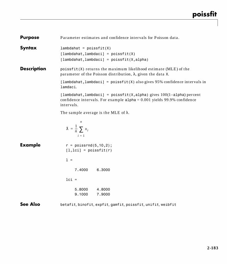
poissfit
2poissfitPurpose Parameter estimates and confidence intervals for Poisson data.
Syntax lambdahat = poissfit(X)
[lambdahat,lambdaci] = poissfit(X)
[lambdahat,lambdaci] = poissfit(X,alpha)
Description poissfit(X) returns the maximum likelihood estimate (MLE) of theparameter of the Poisson distribution, λ, given the data X.
[lambdahat,lambdaci] = poissfit(X) also gives 95% confidence intervals inlamdaci.
[lambdahat,lambdaci] = poissfit(X,alpha) gives 100(1–alpha) percentconfidence intervals. For example alpha = 0.001 yields 99.9% confidenceintervals.
The sample average is the MLE of λ.
Example r = poissrnd(5,10,2);[l,lci] = poissfit(r)
l =
7.4000 6.3000
lci =
5.8000 4.80009.1000 7.9000
See Also betafit, binofit, expfit, gamfit, poissfit, unifit, weibfit
λ1n--- xi
i 1=
n
∑=
2-183
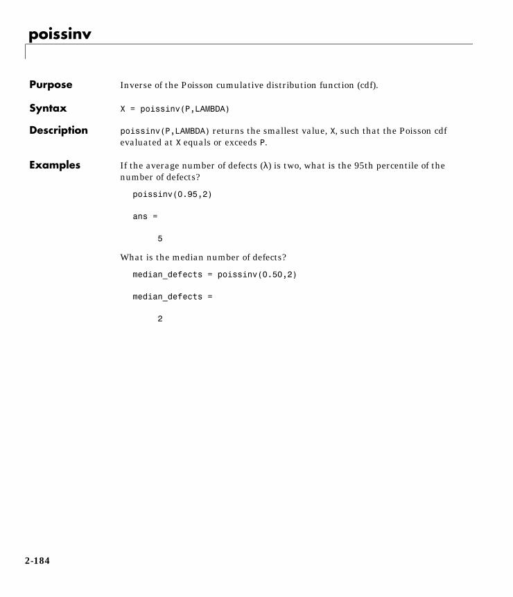
poissinv
2poissinvPurpose Inverse of the Poisson cumulative distribution function (cdf).
Syntax X = poissinv(P,LAMBDA)
Description poissinv(P,LAMBDA) returns the smallest value, X, such that the Poisson cdfevaluated at X equals or exceeds P.
Examples If the average number of defects (λ) is two, what is the 95th percentile of thenumber of defects?
poissinv(0.95,2)
ans =
5
What is the median number of defects?
median_defects = poissinv(0.50,2)
median_defects =
2
2-184
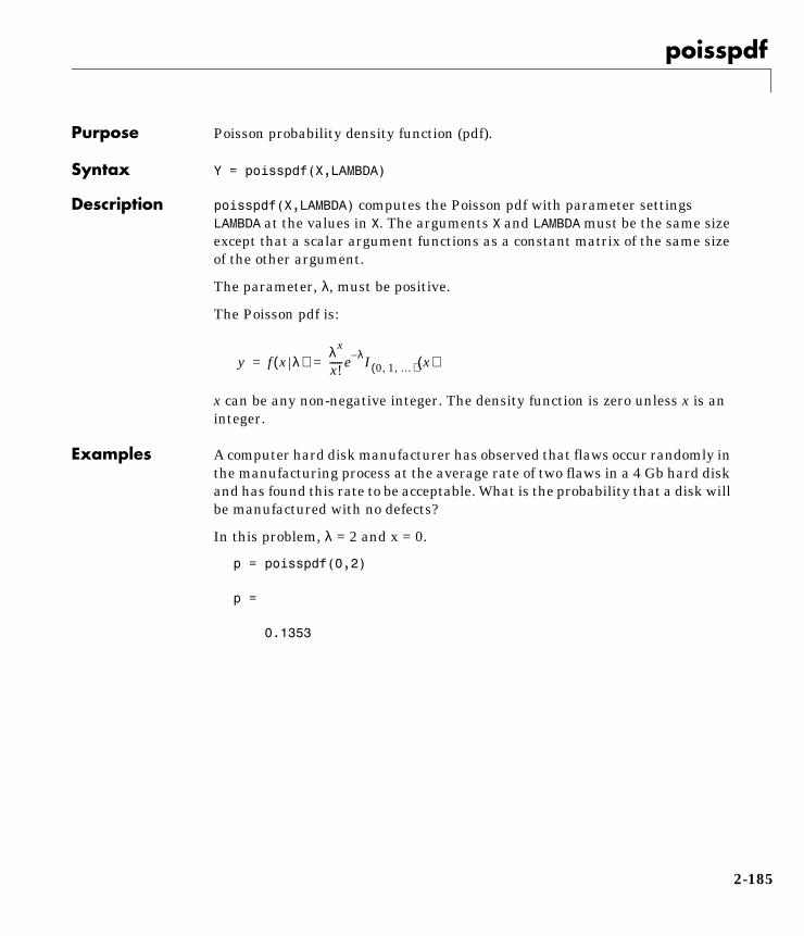
poisspdf
2poisspdfPurpose Poisson probability density function (pdf).
Syntax Y = poisspdf(X,LAMBDA)
Description poisspdf(X,LAMBDA) computes the Poisson pdf with parameter settings LAMBDA at the values in X. The arguments X and LAMBDA must be the same sizeexcept that a scalar argument functions as a constant matrix of the same sizeof the other argument.
The parameter, λ, must be positive.
The Poisson pdf is:
x can be any non-negative integer. The density function is zero unless x is aninteger.
Examples A computer hard disk manufacturer has observed that flaws occur randomly inthe manufacturing process at the average rate of two flaws in a 4 Gb hard diskand has found this rate to be acceptable. What is the probability that a disk willbe manufactured with no defects?
In this problem, λ = 2 and x = 0.
p = poisspdf(0,2)
p =
0.1353
y f x λ( )λx
x!-----e λ– I 0 1 …, ,( ) x( )= =
2-185

poissrnd
2poissrndPurpose Random numbers from the Poisson distribution.
Syntax R = poissrnd(LAMBDA)
R = poissrnd(LAMBDA,m)
R = poissrnd(LAMBDA,m,n)
Description R = poissrnd(LAMBDA) generates Poisson random numbers with mean LAMBDA.The size of R is the size of LAMBDA.
R = poissrnd(LAMBDA,m) generates Poisson random numbers with meanLAMBDA. m is a 1-by-2 vector that contains the row and column dimensions of R.
R = poissrnd(LAMBDA,m,n) generates Poisson random numbers with meanLAMBDA. The scalars m and n are the row and column dimensions of R.
Examples Generate a random sample of 10 pseudo-observations from a Poissondistribution with λ = 2:
lambda = 2;random_sample1 = poissrnd(lambda,1,10)
random_sample1 =
1 0 1 2 1 3 4 2 0 0
random_sample2 = poissrnd(lambda,[1 10])
random_sample2 =
1 1 1 5 0 3 2 2 3 4
random_sample3 = poissrnd(lambda(ones(1,10)))
random_sample3 =
3 2 1 1 0 0 4 0 2 0
2-186
poisstat
2poisstatPurpose Mean and variance for the Poisson distribution.
Syntax M = poisstat(LAMBDA)
[M,V] = poisstat(LAMBDA)
Description M = poisstat(LAMBDA) returns the mean of the Poisson distribution withparameter, LAMBDA. M and LAMBDA match each other in size.
[M,V] = poisstat(LAMBDA) also returns the variance of the Poissondistribution.
For the Poisson distribution:
• the mean is λ.• the variance is λ.
Examples Find the mean and variance for the Poisson distribution with λ = 2:
[m,v] = poisstat([1 2; 3 4])
m =
1 2 3 4
v =
1 2 3 4
2-187
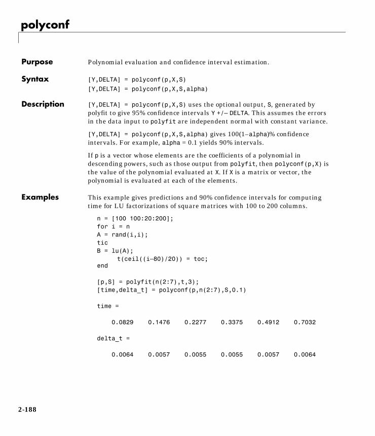
polyconf
2polyconfPurpose Polynomial evaluation and confidence interval estimation.
Syntax [Y,DELTA] = polyconf(p,X,S)
[Y,DELTA] = polyconf(p,X,S,alpha)
Description [Y,DELTA] = polyconf(p,X,S) uses the optional output, S, generated bypolyfit to give 95% confidence intervals Y +/– DELTA. This assumes the errorsin the data input to polyfit are independent normal with constant variance.
[Y,DELTA] = polyconf(p,X,S,alpha) gives 100(1–alpha)% confidenceintervals. For example, alpha = 0.1 yields 90% intervals.
If p is a vector whose elements are the coefficients of a polynomial indescending powers, such as those output from polyfit, then polyconf(p,X) isthe value of the polynomial evaluated at X. If X is a matrix or vector, thepolynomial is evaluated at each of the elements.
Examples This example gives predictions and 90% confidence intervals for computingtime for LU factorizations of square matrices with 100 to 200 columns.
n = [100 100:20:200];for i = nA = rand(i,i);ticB = lu(A);
t(ceil((i–80)/20)) = toc;end
[p,S] = polyfit(n(2:7),t,3);[time,delta_t] = polyconf(p,n(2:7),S,0.1)
time =
0.0829 0.1476 0.2277 0.3375 0.4912 0.7032
delta_t =
0.0064 0.0057 0.0055 0.0055 0.0057 0.0064
2-188
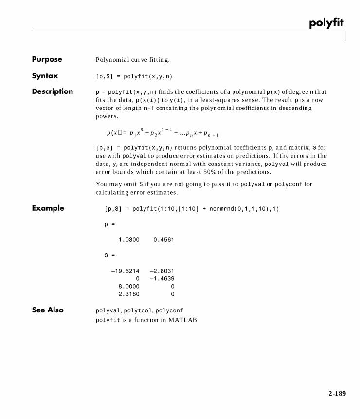
polyfit
2polyfitPurpose Polynomial curve fitting.
Syntax [p,S] = polyfit(x,y,n)
Description p = polyfit(x,y,n) finds the coefficients of a polynomial p(x) of degree n thatfits the data, p(x(i)) to y(i), in a least-squares sense. The result p is a rowvector of length n+1 containing the polynomial coefficients in descendingpowers.
[p,S] = polyfit(x,y,n) returns polynomial coefficients p, and matrix, S foruse with polyval to produce error estimates on predictions. If the errors in thedata, y, are independent normal with constant variance, polyval will produceerror bounds which contain at least 50% of the predictions.
You may omit S if you are not going to pass it to polyval or polyconf forcalculating error estimates.
Example [p,S] = polyfit(1:10,[1:10] + normrnd(0,1,1,10),1)
p =
1.0300 0.4561
S =
–19.6214 –2.8031 0 –1.4639 8.0000 0 2.3180 0
See Also polyval, polytool, polyconfpolyfit is a function in MATLAB.
p x( ) p1xn p2xn 1– …pnx pn 1++ + +=
2-189
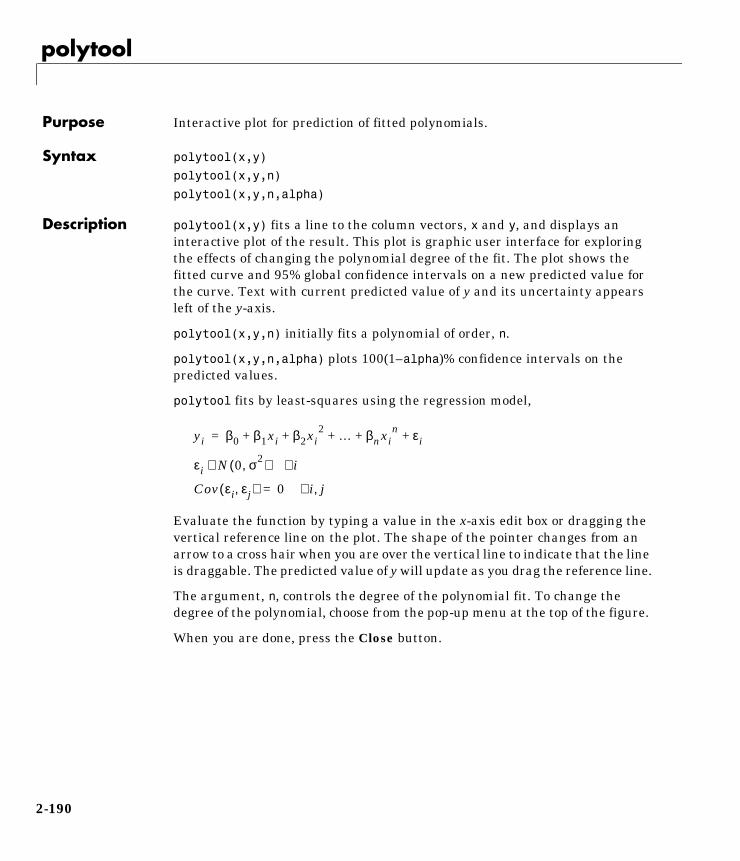
polytool
2polytoolPurpose Interactive plot for prediction of fitted polynomials.
Syntax polytool(x,y)
polytool(x,y,n)
polytool(x,y,n,alpha)
Description polytool(x,y) fits a line to the column vectors, x and y, and displays aninteractive plot of the result. This plot is graphic user interface for exploringthe effects of changing the polynomial degree of the fit. The plot shows thefitted curve and 95% global confidence intervals on a new predicted value forthe curve. Text with current predicted value of y and its uncertainty appearsleft of the y-axis.
polytool(x,y,n) initially fits a polynomial of order, n.
polytool(x,y,n,alpha) plots 100(1–alpha)% confidence intervals on thepredicted values.
polytool fits by least-squares using the regression model,
Evaluate the function by typing a value in the x-axis edit box or dragging thevertical reference line on the plot. The shape of the pointer changes from anarrow to a cross hair when you are over the vertical line to indicate that the lineis draggable. The predicted value of y will update as you drag the reference line.
The argument, n, controls the degree of the polynomial fit. To change thedegree of the polynomial, choose from the pop-up menu at the top of the figure.
When you are done, press the Close button.
yi β0 β1xi β2xi2 … βnxi
n εi+ + ++ +=
εi N 0 σ2,( )∼ i∀
Cov εi εj,( ) 0= i j,∀
2-190
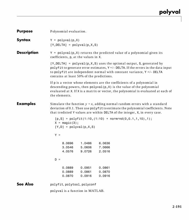
polyval
2polyvalPurpose Polynomial evaluation.
Syntax Y = polyval(p,X)
[Y,DELTA] = polyval(p,X,S)
Description Y = polyval(p,X) returns the predicted value of a polynomial given itscoefficients, p, at the values in X.
[Y,DELTA] = polyval(p,X,S) uses the optional output, S, generated bypolyfit to generate error estimates, Y +/– DELTA. If the errors in the data inputto polyfit are independent normal with constant variance, Y +/– DELTAcontains at least 50% of the predictions.
If p is a vector whose elements are the coefficients of a polynomial indescending powers, then polyval(p,X) is the value of the polynomialevaluated at X. If X is a matrix or vector, the polynomial is evaluated at each ofthe elements.
Examples Simulate the function y = x, adding normal random errors with a standarddeviation of 0.1. Then use polyfit to estimate the polynomial coefficients. Notethat tredicted Y values are within DELTA of the integer, X, in every case.
[p,S] = polyfit(1:10,(1:10) + normrnd(0,0.1,1,10),1);X = magic(3);[Y,D] = polyval(p,X,S)
Y =
8.0696 1.0486 6.0636 3.0546 5.0606 7.0666 4.0576 9.0726 2.0516
D =
0.0889 0.0951 0.0861 0.0889 0.0861 0.0870 0.0870 0.0916 0.0916
See Also polyfit, polytool, polyconf
polyval is a function in MATLAB.
2-191
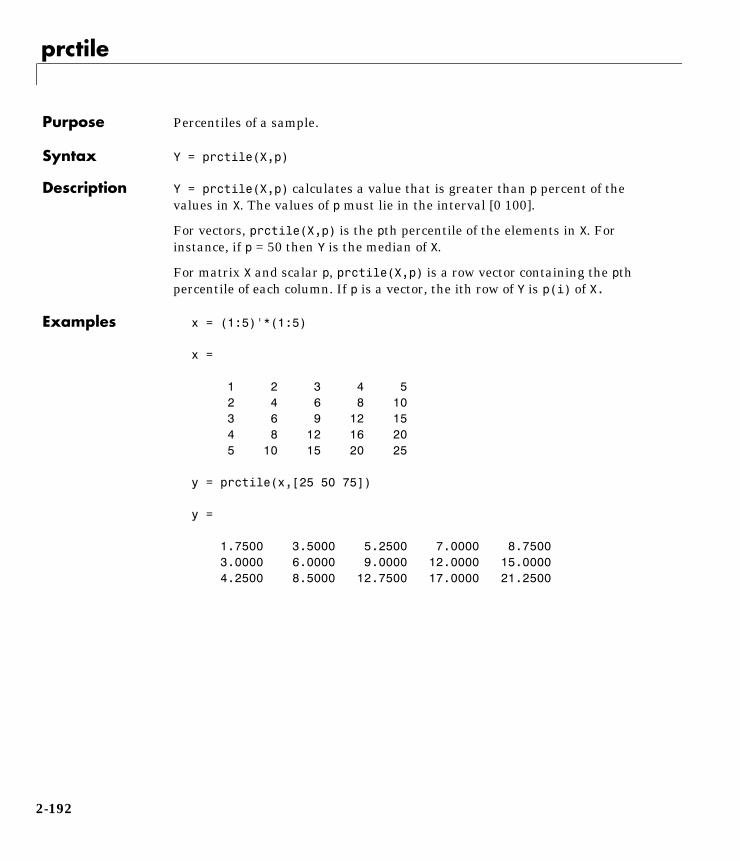
prctile
2prctilePurpose Percentiles of a sample.
Syntax Y = prctile(X,p)
Description Y = prctile(X,p) calculates a value that is greater than p percent of thevalues in X. The values of p must lie in the interval [0 100].
For vectors, prctile(X,p) is the pth percentile of the elements in X. Forinstance, if p = 50 then Y is the median of X.
For matrix X and scalar p, prctile(X,p) is a row vector containing the pth percentile of each column. If p is a vector, the ith row of Y is p(i) of X.
Examples x = (1:5)'*(1:5)
x =
1 2 3 4 5 2 4 6 8 10 3 6 9 12 15 4 8 12 16 20 5 10 15 20 25
y = prctile(x,[25 50 75])
y =
1.7500 3.5000 5.2500 7.0000 8.7500 3.0000 6.0000 9.0000 12.0000 15.0000 4.2500 8.5000 12.7500 17.0000 21.2500
2-192
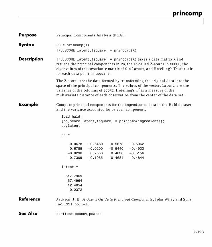
princomp
2princompPurpose Principal Components Analysis (PCA).
Syntax PC = princomp(X)
[PC,SCORE,latent,tsquare] = princomp(X)
Description [PC,SCORE,latent,tsquare] = princomp(X) takes a data matrix X andreturns the principal components in PC, the so-called Z-scores in SCORE, theeigenvalues of the covariance matrix of X in latent, and Hotelling's T2 statisticfor each data point in tsquare.
The Z-scores are the data formed by transforming the original data into thespace of the principal components. The values of the vector, latent, are thevariance of the columns of SCORE. Hotelling's T2 is a measure of themultivariate distance of each observation from the center of the data set.
Example Compute principal components for the ingredients data in the Hald dataset,and the variance accounted for by each component.
load hald;[pc,score,latent,tsquare] = princomp(ingredients);pc,latent
pc =
0.0678 –0.6460 0.5673 –0.5062 0.6785 –0.0200 –0.5440 –0.4933 –0.0290 0.7553 0.4036 –0.5156 –0.7309 –0.1085 –0.4684 –0.4844
latent =
517.7969 67.4964 12.4054 0.2372
Reference Jackson, J. E., A User's Guide to Principal Components, John Wiley and Sons,Inc. 1991. pp. 1–25.
See Also barttest, pcacov, pcares
2-193
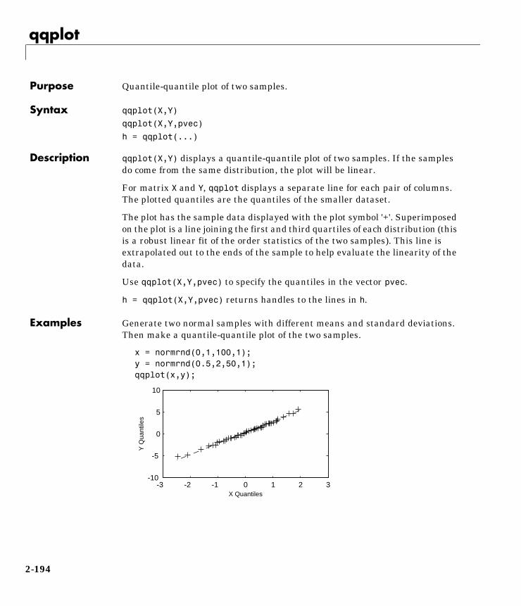
qqplot
2qqplotPurpose Quantile-quantile plot of two samples.
Syntax qqplot(X,Y)
qqplot(X,Y,pvec)
h = qqplot(...)
Description qqplot(X,Y) displays a quantile-quantile plot of two samples. If the samplesdo come from the same distribution, the plot will be linear.
For matrix X and Y, qqplot displays a separate line for each pair of columns.The plotted quantiles are the quantiles of the smaller dataset.
The plot has the sample data displayed with the plot symbol '+'. Superimposedon the plot is a line joining the first and third quartiles of each distribution (thisis a robust linear fit of the order statistics of the two samples). This line isextrapolated out to the ends of the sample to help evaluate the linearity of thedata.
Use qqplot(X,Y,pvec) to specify the quantiles in the vector pvec.
h = qqplot(X,Y,pvec) returns handles to the lines in h.
Examples Generate two normal samples with different means and standard deviations.Then make a quantile-quantile plot of the two samples.
x = normrnd(0,1,100,1);y = normrnd(0.5,2,50,1);qqplot(x,y);
-3 -2 -1 0 1 2 3-10
-5
0
5
10
X Quantiles
Y Q
uant
iles
2-194
random
2randomPurpose Random numbers from a specified distribution.
Syntax y = random('name',A1,A2,A3,m,n)
Description random is a utility routine allowing you to access all the random numbergenerators in the Statistics Toolbox using the name of the distribution as aparameter.
y = random('name',A1,A2,A3,m,n) returns a matrix of random numbers.'name' is a string containing the name of the distribution. A1, A2, and A3 arematrices of distribution parameters. Depending on the distribution some of theparameters may not be necessary.
The arguments containing distribution parameters must all be the same sizeexcept that scalar arguments function as constant matrices of the common sizeof the other arguments.
The last two parameters, d and e, are the size of the matrix, y. If thedistribution parameters are matrices, then these parameters are optional, butthey must match the size of the other matrix arguments (see second example).
Examples rn = random('Normal',0,1,2,4)
rn =
1.1650 0.0751 -0.6965 0.0591 0.6268 0.3516 1.6961 1.7971
rp = random('Poisson',1:6,1,6)
rp =
0 0 1 2 5 7
2-195

randtool
2randtoolPurpose Interactive random number generation using histograms for display.
Syntax randtool
r = randtool('output')
Description The randtool command sets up a graphic user interface for exploring theeffects of changing parameters and sample size on the histogram of randomsamples from the supported probability distributions.
The M-file calls itself recursively using the action and flag parameters. Forgeneral use call randtool without parameters.
To output the current set of random numbers, press the Output button. Theresults are stored in the variable ans. Alternatively, the command
r = randtool('output') places the sample of random numbers in the vector,r.
To sample repetitively from the same distribution, press the Resample button.
To change the distribution function, choose from the pop-up menu of functionsat the top of the figure.
To change the parameter settings, move the sliders or type a value in the editbox under the name of the parameter. To change the limits of a parameter, typea value in the edit box at the top or bottom of the parameter slider.
To change the sample size, type a number in the Sample Size edit box.
When you are done, press the Close button.
For an extensive discussion, see “The disttool Demo” on page 1-125.
See Also disttool
2-196
range
2rangePurpose Sample range.
Syntax y = range(X)
Description range(X) returns the difference between the maximum and the minimum of asample. For vectors, range(x) is the range of the elements. For matrices,range(X) is a row vector containing the range of each column of X.
The range is an easily calculated estimate of the spread of a sample. Outliershave an undue influence on this statistic, which makes it an unreliableestimator.
Example The range of a large sample of standard normal random numbers isapproximately six. This is the motivation for the process capability indices Cpand Cpk in statistical quality control applications.
rv = normrnd(0,1,1000,5);near6 = range(rv)
near6 =
6.1451 6.4986 6.2909 5.8894 7.0002
See Also std, iqr, mad
2-197
ranksum
2ranksumPurpose Wilcoxon rank sum test that two populations are identical.
Syntax p = ranksum(x,y,alpha)
[p,h] = ranksum(x,y,alpha)
Description p = ranksum(x,y,alpha) returns the significance probability that thepopulations generating two independent samples, x and y, are identical. x andy are vectors but can have different lengths; if they are unequal in length, xmust be smaller than y. alpha is the desired level of significance and must bea scalar between zero and one.
[p,h] = ranksum(x,y,alpha) also returns the result of the hypothesis test, h.h is zero if the populations of x and y are not significantly different. h is one ifthe two populations are significantly different.
p is the probability of observing a result equally or more extreme than the oneusing the data (x and y) if the null hypothesis is true. If p is near zero, this castsdoubt on this hypothesis.
Example This example tests the hypothesis of equality of means for two samplesgenerated with poissrnd.
x = poissrnd(5,10,1);y = poissrnd(2,20,1);[p,h] = ranksum(x,y,0.05)
p =
0.0028
h =
1
See Also signrank, signtest, ttest2
2-198
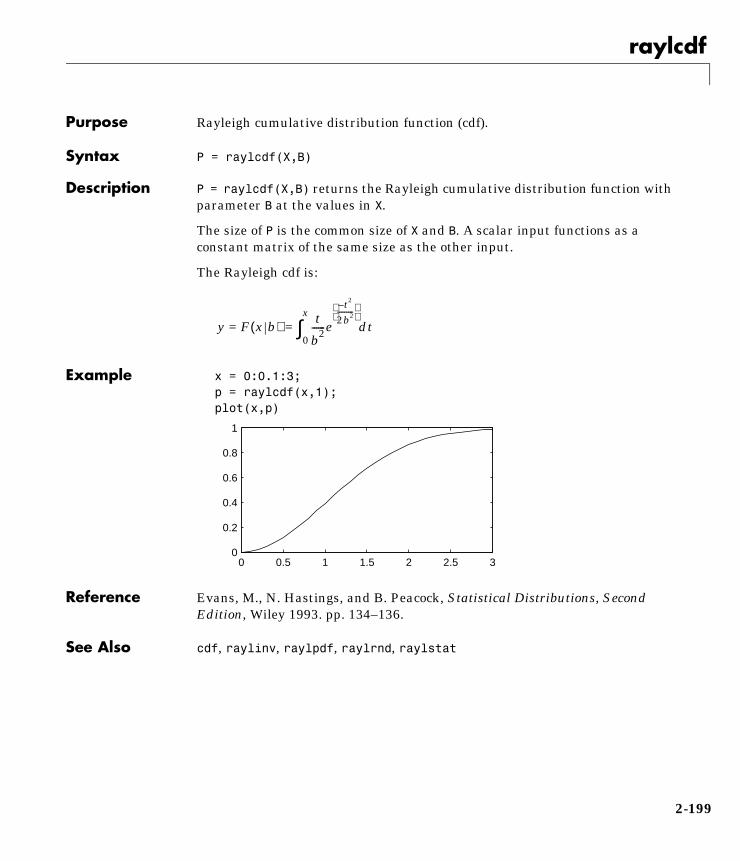
raylcdf
2raylcdfPurpose Rayleigh cumulative distribution function (cdf).
Syntax P = raylcdf(X,B)
Description P = raylcdf(X,B) returns the Rayleigh cumulative distribution function withparameter B at the values in X.
The size of P is the common size of X and B. A scalar input functions as aconstant matrix of the same size as the other input.
The Rayleigh cdf is:
Example x = 0:0.1:3;p = raylcdf(x,1);plot(x,p)
Reference Evans, M., N. Hastings, and B. Peacock, Statistical Distributions, SecondEdition, Wiley 1993. pp. 134–136.
See Also cdf, raylinv, raylpdf, raylrnd, raylstat
y F x b( ) t
b2------0
x
∫ e
t2–
2b2---------
= = dt
0 0.5 1 1.5 2 2.5 30
0.2
0.4
0.6
0.8
1
2-199
raylinv
2raylinvPurpose Inverse of the Rayleigh cumulative distribution function.
Syntax X = raylinv(P,B)
Description X = raylinv(P,B) returns the inverse of the Rayleigh cumulative distributionfunction with parameter B at the probabilities in P.
The size of X is the common size of P and B. A scalar input functions as aconstant matrix of the same size as the other input.
Example x = raylinv(0.9,1)
x =
2.1460
See Also icdf, raylcdf, raylpdf, raylrnd, raylstat
2-200
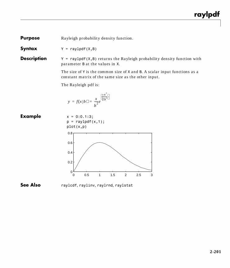
raylpdf
2raylpdfPurpose Rayleigh probability density function.
Syntax Y = raylpdf(X,B)
Description Y = raylpdf(X,B) returns the Rayleigh probability density function withparameter B at the values in X.
The size of Y is the common size of X and B. A scalar input functions as aconstant matrix of the same size as the other input.
The Rayleigh pdf is:
Example x = 0:0.1:3;p = raylpdf(x,1);plot(x,p)
See Also raylcdf, raylinv, raylrnd, raylstat
y f x b( )x
b2------e
x2–
2b2---------
= =
0 0.5 1 1.5 2 2.5 30
0.2
0.4
0.6
0.8
2-201
raylrnd
2raylrndPurpose Random matrices from the Rayleigh distribution.
Syntax R = raylrnd(B)
R = raylrnd(B,m)
R = raylrnd(B,m,n)
Description R = raylrnd(B) returns a matrix of random numbers chosen from the Rayleighdistribution with parameter B. The size of R is the size of B.
R = raylrnd(B,m) returns a matrix of random numbers chosen from theRayleigh distribution with parameter B. m is a 1-by-2 vector that contains therow and column dimensions of R.
R = raylrnd(B,m,n) returns a matrix of random numbers chosen from theRayleigh distribution with parameter B. The scalars m and n are the row andcolumn dimensions of R.
Example r = raylrnd(1:5)
r =
1.7986 0.8795 3.3473 8.9159 3.5182
See Also random, raylcdf, raylinv, raylpdf, raylstat
2-202
raylstat
2raylstatPurpose Mean and variance for the Rayleigh distribution.
Syntax M = raylstat(B)
[M,V] = raylstat(B)
Description [M,V] = raylstat(B) returns the mean and variance of the Rayleighdistribution with parameter B.
For the Rayleigh distribution:
• The mean is .
• The variance is .
Example [mn,v] = raylstat(1)
mn =
1.2533
v =
0.4292
See Also raylcdf, raylinv, raylpdf, raylrnd
bπ2---
12---
4 π–2------------b2
2-203

rcoplot
2rcoplotPurpose Residual case order plot.
Syntax rcoplot(r,rint)
Description rcoplot(r,rint) displays an errorbar plot of the confidence intervals on theresiduals from a regression. The residuals appear in the plot in case order. rand rint are outputs from the regress function.
Example X = [ones(10,1) (1:10)'];y = X ∗ [10;1] + normrnd(0,0.1,10,1);[b,bint,r,rint] = regress(y,X,0.05);rcoplot(r,rint);
The figure shows a plot of the residuals with error bars showing 95% confidenceintervals on the residuals. All the error bars pass through the zero line,indicating that there are no outliers in the data.
See Also regress
0 2 4 6 8 10
-0.2
-0.1
0
0.1
0.2
Res
idua
ls
Case Number
2-204
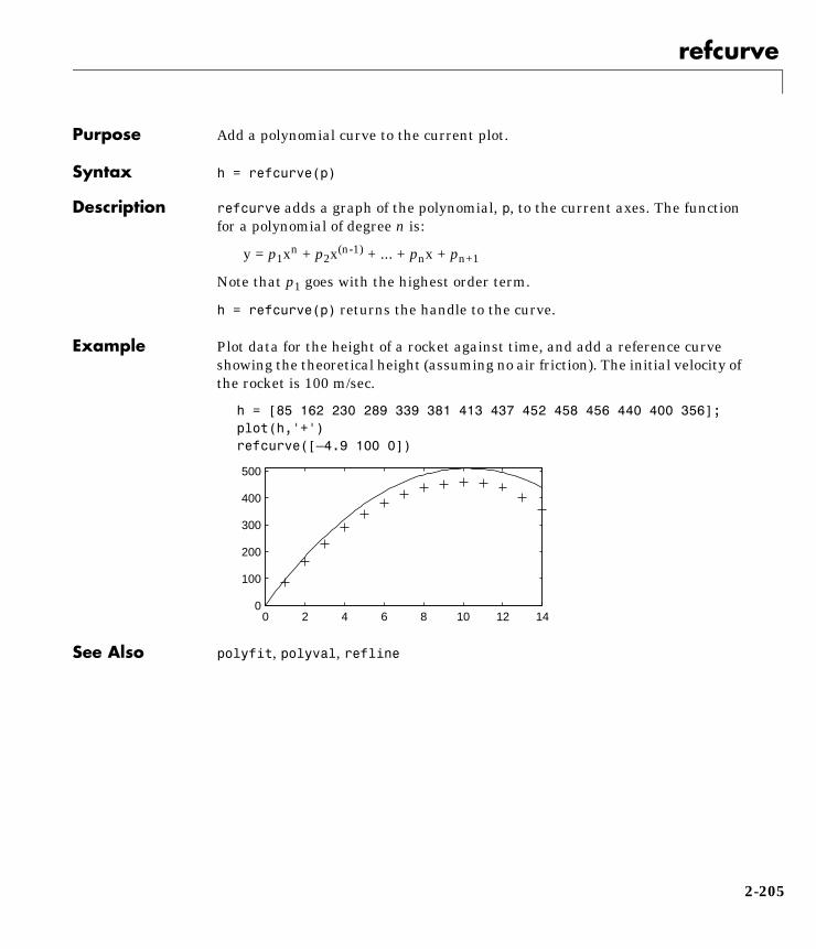
refcurve
2refcurvePurpose Add a polynomial curve to the current plot.
Syntax h = refcurve(p)
Description refcurve adds a graph of the polynomial, p, to the current axes. The functionfor a polynomial of degree n is:
y = p1xn + p2x(n-1) + ... + pnx + pn+1
Note that p1 goes with the highest order term.
h = refcurve(p) returns the handle to the curve.
Example Plot data for the height of a rocket against time, and add a reference curveshowing the theoretical height (assuming no air friction). The initial velocity ofthe rocket is 100 m/sec.
h = [85 162 230 289 339 381 413 437 452 458 456 440 400 356];plot(h,'+')refcurve([–4.9 100 0])
See Also polyfit, polyval, refline
0 2 4 6 8 10 12 140
100
200
300
400
500
2-205
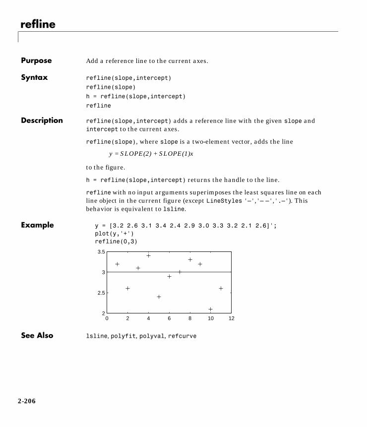
refline
2reflinePurpose Add a reference line to the current axes.
Syntax refline(slope,intercept)
refline(slope)
h = refline(slope,intercept)
refline
Description refline(slope,intercept) adds a reference line with the given slope andintercept to the current axes.
refline(slope), where slope is a two-element vector, adds the line
y = SLOPE(2) + SLOPE(1)x
to the figure.
h = refline(slope,intercept) returns the handle to the line.
refline with no input arguments superimposes the least squares line on eachline object in the current figure (except LineStyles '–','– –','.–'). Thisbehavior is equivalent to lsline.
Example y = [3.2 2.6 3.1 3.4 2.4 2.9 3.0 3.3 3.2 2.1 2.6]';plot(y,'+')refline(0,3)
See Also lsline, polyfit, polyval, refcurve
0 2 4 6 8 10 122
2.5
3
3.5
2-206

regress
2regressPurpose Multiple linear regression.
Syntax b = regress(y,X)
[b,bint,r,rint,stats] = regress(y,X)
[b,bint,r,rint,stats] = regress(y,X,alpha)
Description b = regress(y,X) returns the least squares fit of y on X.
regress solves the linear model
for β, where:
• y is an nx1 vector of observations,
• X is an nxp matrix of regressors,
• β is a px1 vector of parameters, and
• ε is an nx1 vector of random disturbances.
[b,bint,r,rint,stats] = regress(y,X) returns an estimate of β in b, a 95%confidence interval for β, in the p-by-2 vector bint. The residuals are in r anda 95% confidence interval for each residual, is in the n-by-2 vector rint. Thevector, stats, contains the R2 statistic along with the F and p values for theregression.
[b,bint,r,rint,stats] = regress(y,X,alpha) gives 100(1-alpha)%confidence intervals for bint and rint. For example, alpha = 0.2 gives 80%confidence intervals.
Examples Suppose the true model is:
where I is the identity matrix.
y Xβ ε+=
ε N 0 σ2I,( )∼
y 10 x ε+ +=
ε N 0 0.01I,( )∼
2-207
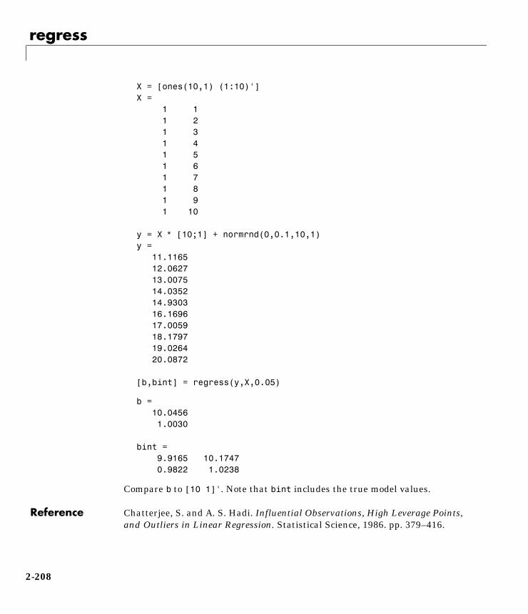
regress
X = [ones(10,1) (1:10)']X = 1 1 1 2 1 3 1 4 1 5 1 6 1 7 1 8 1 9 1 10
y = X ∗ [10;1] + normrnd(0,0.1,10,1)y = 11.1165 12.0627 13.0075 14.0352 14.9303 16.1696 17.0059 18.1797 19.0264 20.0872
[b,bint] = regress(y,X,0.05)
b = 10.0456 1.0030
bint = 9.9165 10.1747 0.9822 1.0238
Compare b to [10 1]'. Note that bint includes the true model values.
Reference Chatterjee, S. and A. S. Hadi. Influential Observations, High Leverage Points,and Outliers in Linear Regression. Statistical Science, 1986. pp. 379–416.
2-208
regstats
2regstatsPurpose Regression diagnostics graphical user interface.
Syntax regstats(responses,DATA)
regstats(responses,DATA,'model')
Description regstats(responses,DATA) generates regression diagnostics for a linearadditive model with a constant term. The dependent variable is the vector,responses. Values of the independent variables are in the matrix, DATA.
The function creates a figure with a group of checkboxes that save diagnosticstatistics to the base workspace using variable names you can specify.
regstats(responses,data,'model') controls the order of the regressionmodel. 'model' can be one of these strings:
• 'interaction' – includes constant, linear, and cross product terms.
• 'quadratic' – interactions plus squared terms.
• 'purequadratic' – includes constant, linear and squared terms.
The literature suggests many diagnostic statistics for evaluating multiplelinear regression. regstats provides these diagnostics:
• Q from QR decomposition.
• R from QR decomposition.
• Regression coefficients.
• Covariance of regression coefficients.
• Fitted values of the response data.
• Residuals.
• Mean squared error.
• Leverage.
• “Hat” matrix.
• Delete-1 variance.
• Delete-1 coefficients.
• Standardized residuals.
• Studentized residuals.
• Change in regression coefficients.
2-209
regstats
• Change in fitted values.
• Scaled change in fitted values.
• Change in covariance.
• Cook's distance.
For more detail press the Help button in the regstats window. This displaysa hypertext help that gives formulae and interpretations for each of theseregression diagnostics.
Algorithm The usual regression model is: y = Xβ + εwhere:
• y is an n by 1 vector of responses.
• X is an n by p matrix of predictors.
• β is an p by 1 vector of parameters.
• ε is an n by 1 vector of random disturbances.
Let X = Q*R where Q and R come from a QR Decomposition of X. Q is orthogonaland R is triangular. Both of these matrices are useful for calculating manyregression diagnostics (Goodall 1993).
The standard textbook equation for the least squares estimator of β is:
However, this definition has poor numeric properties. Particularly dubious isthe computation of , which is both expensive and imprecise.
Numerically stable MATLAB code for β is: b = R\(Q'*y);
Reference Goodall, C. R. (1993). Computation using the QR decomposition. Handbook inStatistics, Volume 9. Statistical Computing (C. R. Rao, ed.). Amsterdam, NLElsevier/North-Holland.
See Also leverage, stepwise, regress
β b X'X( )1–
X'y= =
X'X( )1–
2-210
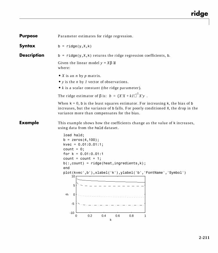
ridge
2ridgePurpose Parameter estimates for ridge regression.
Syntax b = ridge(y,X,k)
Description b = ridge(y,X,k) returns the ridge regression coefficients, b.
Given the linear model y = Xβ + εwhere:
• X is an n by p matrix.
• y is the n by 1 vector of observations.
• k is a scalar constant (the ridge parameter).
The ridge estimator of β is: .
When k = 0, b is the least squares estimator. For increasing k, the bias of bincreases, but the variance of b falls. For poorly conditioned X, the drop in thevariance more than compensates for the bias.
Example This example shows how the coefficients change as the value of k increases,using data from the hald dataset.
load hald;b = zeros(4,100);kvec = 0.01:0.01:1;count = 0;for k = 0.01:0.01:1count = count + 1;b(:,count) = ridge(heat,ingredients,k);endplot(kvec',b'),xlabel('k'),ylabel('b','FontName','Symbol')
b X'X kI+( )1–
X'y=
0 0.2 0.4 0.6 0.8 1-10
-5
0
5
10
k
β
2-211

ridge
See Also regress, stepwise
2-212
rowexch
2rowexchPurpose D-optimal design of experiments – row exchange algorithm.
Syntax settings = rowexch(nfactors,nruns)
[settings,X] = rowexch(nfactors,nruns)
[settings,X] = rowexch(nfactors,nruns,'model')
Description settings = rowexch(nfactors,nruns) generates the factor settings matrix,settings, for a D-Optimal design using a linear additive model with a constantterm. settings has nruns rows and nfactors columns.
[settings,X] = rowexch(nfactors,nruns) also generates the associateddesign matrix, X.
[settings,X] = rowexch(nfactors,nruns,'model') produces a design forfitting a specified regression model. The input, 'model', can be one of thesestrings:
• 'interaction' – includes constant, linear, and cross product terms.
• 'quadratic' – interactions plus squared terms.
• 'purequadratic' – includes constant, linear and squared terms.
Example This example illustrates that the D-optimal design for three factors in eightruns, using an interactions model, is a two level full-factorial design.
s = rowexch(3,8,'interaction')
s =
–1 –1 1 1 –1 –1 1 –1 1 –1 –1 –1 –1 1 1 1 1 1 –1 1 –1 1 1 –1
See Also cordexch, daugment, dcovary, fullfact, ff2n, hadamard
2-213

rsmdemo
2rsmdemoPurpose Demo of design of experiments and surface fitting.
Syntax rsmdemo
Description rsmdemo creates a GUI that simulates a chemical reaction. To start, you havea budget of 13 test reactions. Try to find out how changes in each reactant affectthe reaction rate. Determine the reactant settings that maximize the reactionrate. Estimate the run-to-run variability of the reaction. Now run a designedexperiment using the model pop-up. Compare your previous results with theoutput from response surface modeling or nonlinear modeling of the reaction.The GUI has the following elements:
• A Run button to perform one reactor run at the current settings.
• An Export button to export the X and y data to the base workspace.
• Three sliders with associated data entry boxes to control the partialpressures of the chemical reactants: Hydrogen, n-Pentane, and Isopentane.
• A text box to report the reaction rate.
• A text box to keep track of the number of test reactions you have left.
Example See “The rsmdemo Demo” on page 1-131.
See Also rstool, nlintool, cordexch
2-214
rstool
2rstoolPurpose Interactive fitting and visualization of a response surface.
Syntax rstool(x,y)
rstool(x,y,'model')
rstool(x,y,'model',alpha,'xname','yname')
Description rstool(x,y) displays an interactive prediction plot with 95% global confidenceintervales. This plot results from a multiple regression of (X,y) data using alinear additive model.
rstool(x,y,'model') allows control over the initial regression model. 'model'can be one of the following strings:
• 'interaction' – includes constant, linear, and cross product terms.
• 'quadratic' – interactions plus squared terms.
• 'purequadratic' – includes constant, linear and squared terms.
rstool(x,y,'model',alpha) plots 100(1 – alpha)% global confidence intervalfor predictions as two red curves. For example, alpha = 0.01 gives 99%confidence intervals.
rstool displays a “vector” of plots, one for each column of the matrix of inputs,x. The response variable, y, is a column vector that matches the number of rowsin x.
rstool(x,y,'model',alpha,'xname','yname') labels the graph using thestring matrix 'xname' for the labels to the x-axes and the string, 'yname', tolabel the y-axis common to all the plots.
Drag the dotted white reference line and watch the predicted values updatesimultaneously. Alternatively, you can get a specific prediction by typing thevalue of x into an editable text field. Use the pop-up menu labeled Model tointeractively change the model. Use the pop-up menu labeled Export to movespecified variables to the base workspace.
Example See “Quadratic Response Surface Models” on page 1-73.
See Also nlintool
2-215
schart
2schartPurpose Chart of standard deviation for Statistical Process Control.
Syntax schart(DATA,conf)
schart(DATA,conf,specs)
schart(DATA,conf,specs)
[outliers,h] = schart(DATA,conf,specs)
Description schart(data) displays an S chart of the grouped responses in DATA. The rowsof DATA contain replicate observations taken at a given time. The rows must bein time order. The upper and lower control limits are a 99% confidence intervalon a new observation from the process. So, roughly 99% of the plotted pointsshould fall between the control limits.
schart(DATA,conf) allows control of the the confidence level of the upper andlower plotted confidence limits. For example, conf = 0.95 plots 95% confidenceintervals.
schart(DATA,conf,specs) plots the specification limits in the two elementvector, specs.
[outliers,h] = schart(data,conf,specs) returns outliers, a vector ofindices to the rows where the mean of DATA is out of control, and h, a vector ofhandles to the plotted lines.
Example This example plots an S chart of measurements on newly machined parts,taken at one hour intervals for 36 hours. Each row of the runout matrixcontains the measurements for 4 parts chosen at random. The values indicate,
2-216
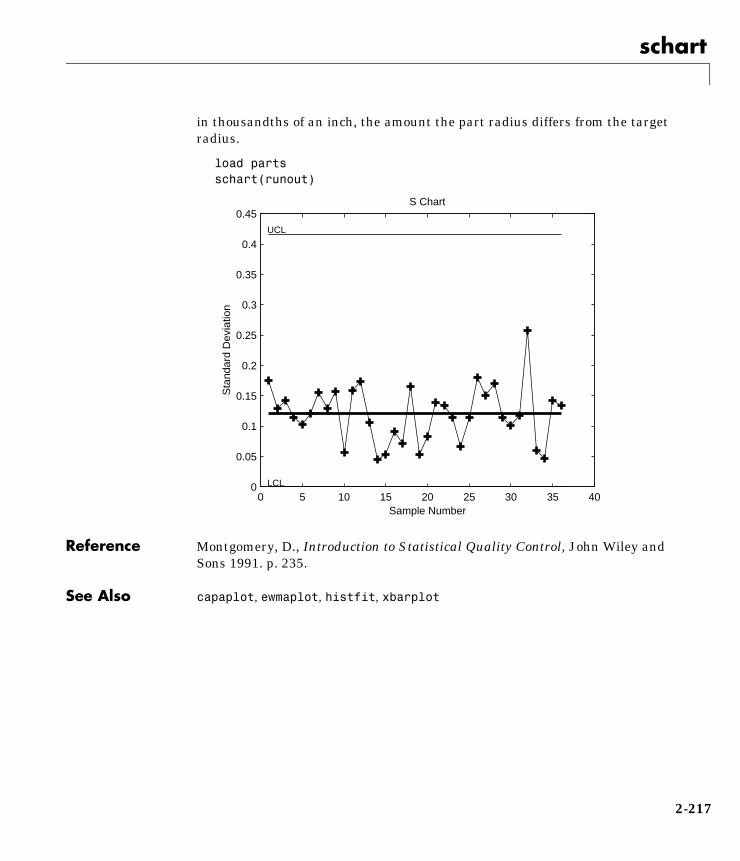
schart
in thousandths of an inch, the amount the part radius differs from the targetradius.
load partsschart(runout)
Reference Montgomery, D., Introduction to Statistical Quality Control, John Wiley andSons 1991. p. 235.
See Also capaplot, ewmaplot, histfit, xbarplot
0 5 10 15 20 25 30 35 400
0.05
0.1
0.15
0.2
0.25
0.3
0.35
0.4
0.45S Chart
Sample Number
Sta
ndar
d D
evia
tion
UCL
LCL
2-217

signrank
2signrankPurpose Wilcoxon signed rank test of equality of medians.
Syntax p = signrank(x,y,alpha)
[p,h] = signrank(x,y,alpha)
Description p = signrank(x,y,alpha) returns the significance probability that themedians of two matched samples, x and y, are equal. x and y must be vectorsof equal length. alpha is the desired level of significance, and must be a scalarbetween zero and one.
[p,h] = signrank(x,y,alpha) also returns the result of the hypothesis test,h. h is zero if the difference in medians of x and y is not significantly differentfrom zero. h is one if the two medians are significantly different.
p is the probability of observing a result equally or more extreme than the oneusing the data (x and y) if the null hypothesis is true. p is calculated using therank values for the differences between corresponding elements in x and y. If pis near zero, this casts doubt on this hypothesis.
Example This example tests the hypothesis of equality of means for two samplesgenerated with normrnd. The samples have the same theoretical mean butdifferent standard deviations.
x = normrnd(0,1,20,1);y = normrnd(0,2,20,1);[p,h] = signrank(x,y,0.05)
p =
0.2568
h =
0
See Also ranksum, signtest, ttest
2-218

signtest
2signtestPurpose Sign test for paired samples.
Syntax p = signtest(x,y,alpha)
[p,h] = signtest(x,y,alpha)
Description p = signtest(x,y,alpha) returns the significance probability that themedians of two matched samples, x and y, are equal. x and y must be vectorsof equal length. y may also be a scalar; in this case, signtest computes theprobability that the median of x is different from the constant, y. alpha is thedesired level of significance and must be a scalar between zero and one.
[p,h] = signtest(x,y,alpha) also returns the result of the hypothesis test,h. h is zero if the difference in medians of x and y is not significantly differentfrom zero. h is one if the two medians are significantly different.
p is the probability of observing a result equally or more extreme than the oneusing the data (x and y) if the null hypothesis is true. p is calculated using thesigns (plus or minus) of the differences between corresponding elements in xand y. If p is near zero, this casts doubt on this hypothesis.
Example This example tests the hypothesis of equality of means for two samplesgenerated with normrnd. The samples have the same theoretical mean butdifferent standard deviations.
x = normrnd(0,1,20,1);y = normrnd(0,2,20,1);[p,h] = signtest(x,y,0.05)
p =
0.8238
h =
0
See Also ranksum, signrank, ttest
2-219
skewness
2skewnessPurpose Sample skewness.
Syntax y = skewness(X)
Description skewness(X) returns the sample skewness of X. For vectors, skewness(x) is theskewness of the elements of x. For matrices, skewness(X) is a row vectorcontaining the sample skewness of each column.
Skewness is a measure of the asymmetry of the data around the sample mean.If skewness is negative, the data are spread out more to the left of the meanthan to the right. If skewness is positive, the data are spread out more to theright. The skewness of the normal distribution (or any perfectly symmetricdistribution) is zero.
The skewness of a distribution is defined as:
where E(x) is the expected value of x.
Example X = randn([5 4])
X =
1.1650 1.6961 –1.4462 –0.3600 0.6268 0.0591 –0.7012 –0.1356 0.0751 1.7971 1.2460 –1.3493 0.3516 0.2641 –0.6390 –1.2704 –0.6965 0.8717 0.5774 0.9846
y = skewness(X)
y =
–0.2933 0.0482 0.2735 0.4641
See Also kurtosis, mean, moment, std, var
yE x µ–( )3
σ3------------------------=
2-220
squareform
2squareform
Purpose Reformat the output of pdist into a square matrix.
Syntax S = squareform(Y)
Description S = squareform(Y) reformats the distance information returned by pdist froma vector into a square matrix. In this format, S(i,j) denotes the distancebetween the i and j observations in the original data.
See Also See pdist.
2-221
std
2stdPurpose Standard deviation of a sample.
Syntax y = std(X)
Description std(X) computes the sample standard deviation of the data in X. For vectors,std(x) is the standard deviation of the elements in x. For matrices, std(X) isa row vector containing the standard deviation of each column of X.
std(X) normalizes by n–1 where n is the sequence length. For normallydistributed data, the square of the standard deviation is the minimum varianceunbiased estimator of σ 2 (the second parameter).
The standard deviation is
where the sample average is .
Examples In each column, the expected value of y is one.
x = normrnd(0,1,100,6);y = std(x)
y =
0.9536 1.0628 1.0860 0.9927 0.9605 1.0254
y = std(–1:2:1)
y =
1.4142
See Also cov, varstd is a function in MATLAB.
s1
n 1–------------- xi x–( )2
i 1=
n
∑
12---
=
x1n--- xi∑=
2-222

stepwise
2stepwisePurpose Interactive environment for stepwise regression.
Syntax stepwise(X,y)
stepwise(X,y,inmodel)
stepwise(X,y,inmodel,alpha)
Description stepwise(X,y) fits a regression model of y on the columns of X. It displaysthree figure windows for interactively controlling the stepwise addition andremoval of model terms.
stepwise(X,y,inmodel) allows control of the terms in the original regressionmodel. The values of vector, inmodel, are the indices of the columns of thematrix, X, to include in the initial model.
stepwise(X,y,inmodel,alpha) allows control of the length confidenceintervals on the fitted coefficients. alpha is the significance for testing eachterm in the model. By default, alpha = 1 – (1 – 0.025)(1/p) where p is the numberof columns in X. This translates to plotted 95% simultaneous confidenceintervals (Bonferroni) for all the coefficients.
The least squares coefficient is plotted with a green filled circle. A coefficient isnot significantly different from zero if its confidence interval crosses the whitezero line. Significant model terms are plotted using solid lines. Terms notsignificantly different from zero are plotted with dotted lines.
Click on the confidence interval lines to toggle the state of the modelcoefficients. If the confidence interval line is green the term is in the model. Ifthe the confidence interval line is red the term is not in the model.
Use the pop-up menu, Export, to move variables to the base workspace.
Example See “Stepwise Regression” on page 1-75.
Reference Draper, N. and H. Smith, Applied Regression Analysis, Second Edition, JohnWiley and Sons, Inc. 1981 pp. 307–312.
See Also regstats, regress, rstool
2-223
surfht
2surfhtPurpose Interactive contour plot.
Syntax surfht(Z)
surfht(x,y,Z)
Description surfht(Z) is an interactive contour plot of the matrix Z treating the values inZ as height above the plane. The x-values are the column indices of Z while they-values are the row indices of Z.
surfht(x,y,Z), where x and y are vectors specify the x and y-axes on thecontour plot. The length of x must match the number of columns in Z, and thelength of y must match the number of rows in Z.
There are vertical and horizontal reference lines on the plot whose intersectiondefines the current x-value and y-value. You can drag these dotted whitereference lines and watch the interpolated z-value (at the top of the plot)update simultaneously. Alternatively, you can get a specific interpolatedz-value by typing the x-value and y-value into editable text fields on the x-axisand y-axis respectively.
2-224
tabulate
2tabulatePurpose Frequency table.
Syntax table = tabulate(x)
tabulate(x)
Description table = tabulate(x) takes a vector of positive integers, x, and returns amatrix, table.
The first column of table contains the values of x. The second contains thenumber of instances of this value. The last column contains the percentage ofeach value.
tabulate with no output arguments displays a formatted table in thecommand window.
Example tabulate([1 2 4 4 3 4])
Value Count Percent 1 1 16.67% 2 1 16.67% 3 1 16.67% 4 3 50.00%
See Also pareto
2-225

tblread
2tblreadPurpose Read tabular data from the file system.
Syntax [data,varnames,casenames] = tblread
[data,varnames,casenames] = tblread('filename')
[data,varnames,casenames] = tblread('filename','delimiter')
Description [data,varnames,casenames] = tblread displays the File Open dialog box forinteractive selection of the tabular data file. The file format has variable namesin the first row, case names in the first column and data starting in the (2,2)position.
[data,varnames,casenames] = tblread(filename) allows command linespecification of the name of a file in the current directory, or the completepathname of any file.
[data,varnames,casenames] = tblread(filename,'delimiter') allowsspecification of the field 'delimiter' in the file. Accepted values are 'tab','space', or 'comma'.
tblread returns the data read in three values.
Return Value
Description
data Numeric matrix with a value for each variable-case pair.
varnames String matrix containing the variable names in the firstrow.
casenames String matrix containing the names of each case in the firstcolumn.
2-226

tblread
Example [data,varnames,casenames] = tblread('sat.dat')
data =
470 530 520 480
varnames =
Male Female
casenames =
Verbal Quantitative
See Also caseread, tblwrite
2-227
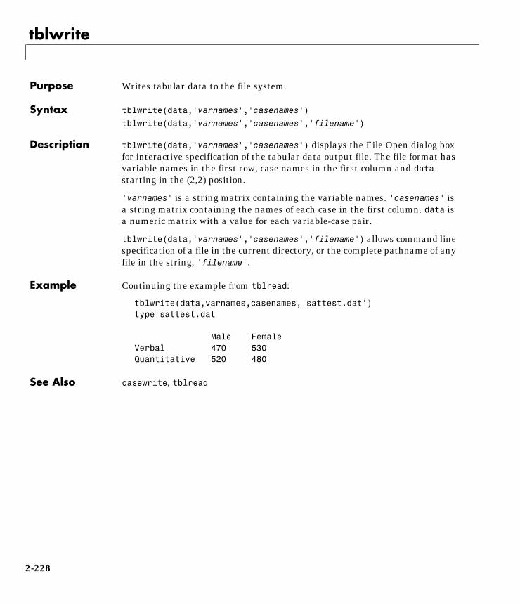
tblwrite
2tblwritePurpose Writes tabular data to the file system.
Syntax tblwrite(data,'varnames','casenames')
tblwrite(data,'varnames','casenames','filename')
Description tblwrite(data,'varnames','casenames') displays the File Open dialog boxfor interactive specification of the tabular data output file. The file format hasvariable names in the first row, case names in the first column and datastarting in the (2,2) position.
'varnames' is a string matrix containing the variable names. 'casenames' isa string matrix containing the names of each case in the first column. data isa numeric matrix with a value for each variable-case pair.
tblwrite(data,'varnames','casenames','filename') allows command linespecification of a file in the current directory, or the complete pathname of anyfile in the string, 'filename'.
Example Continuing the example from tblread:
tblwrite(data,varnames,casenames,'sattest.dat')type sattest.dat
Male FemaleVerbal 470 530Quantitative 520 480
See Also casewrite, tblread
2-228

tcdf
2tcdfPurpose Student’s t cumulative distribution function (cdf).
Syntax P = tcdf(X,V)
Description tcdf(X,V) computes Student’s t cdf with V degrees of freedom at the values inX. The arguments X and V must be the same size except that a scalar argumentfunctions as a constant matrix of the same size of the other argument.
The parameter, V, is a positive integer.
The t cdf is:
The result, p, is the probability that a single observation from the tdistribution with ν degrees of freedom will fall in the interval (–∞ x].
Examples Suppose 10 samples of Guinness beer have a mean alcohol content of 5.5% byvolume and the standard deviation of these samples is 0.5%. What is theprobability that the true alcohol content of Guinness beer is less than 5%?
t = (5.0 – 5.5) / 0.5;probability = tcdf(t,10 – 1)
probability =
0.1717
p F x ν( )Γ
ν 1+2------------
Γν2---
---------------------
1νπ
----------1
1t2
ν-----+
ν 1+2------------
------------------------------ td∞–
x
∫= =
2-229

tinv
2tinvPurpose Inverse of the Student’s t cumulative distribution function (cdf).
Syntax X = tinv(P,V)
Description tinv(P,V) computes the inverse of Student’s t cdf with parameter V for theprobabilities in P. The arguments P and V must be the same size except that ascalar argument functions as a constant matrix of the size of the otherargument.
The degrees of freedom, V, must be a positive integer and P must lie in theinterval [0 1].
The t inverse function in terms of the t cdf is
where
The result, x, is the solution of the integral equation of the t cdf with parameterν where you supply the desired probability p.
Examples What is the 99th percentile of the t distribution for one to six degrees offreedom?
percentile = tinv(0.99,1:6)
percentile =
31.8205 6.9646 4.5407 3.7469 3.3649 3.1427
x F 1– p ν( ) x:F x ν( ) p={ }= =
p F x ν( )Γ
ν 1+2------------
Γν2---
---------------------
1νπ
----------1
1t2
ν-----+
ν 1+2------------
------------------------------ td∞–
x
∫= =
2-230

tpdf
2tpdfPurpose Student’s t probability density function (pdf).
Syntax Y = tpdf(X,V)
Description tpdf(X,V) computes Student’s t pdf with parameter V at the values in X. Thearguments X and V must be the same size except that a scalar argumentfunctions as a constant matrix of the same size of the other argument.
The degrees of freedom, V, must be a positive integer.
Student’s t pdf is:
Examples The mode of the t distribution is at x = 0. This example shows that the value ofthe function at the mode is an increasing function of the degrees of freedom.
tpdf(0,1:6)
ans =
0.3183 0.3536 0.3676 0.3750 0.3796 0.3827
The t distribution converges to the standard normal distribution as the degreesof freedom approaches infinity. How good is the approximation for v = 30?
difference = tpdf(–2.5:2.5,30) – normpdf(–2.5:2.5)
difference =
0.0035 –0.0006 –0.0042 –0.0042 –0.0006 0.0035
y f x ν( )Γ
ν 1+2------------
Γν2---
---------------------
1νπ
----------1
1x2
ν-----+
ν 1+2------------
-------------------------------= =
2-231
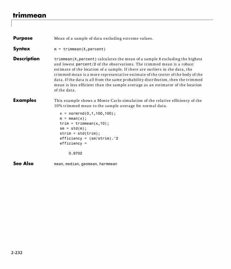
trimmean
2trimmeanPurpose Mean of a sample of data excluding extreme values.
Syntax m = trimmean(X,percent)
Description trimmean(X,percent) calculates the mean of a sample X excluding the highestand lowest percent/2 of the observations. The trimmed mean is a robustestimate of the location of a sample. If there are outliers in the data, thetrimmed mean is a more representative estimate of the center of the body of thedata. If the data is all from the same probability distribution, then the trimmedmean is less efficient than the sample average as an estimator of the locationof the data.
Examples This example shows a Monte Carlo simulation of the relative efficiency of the10% trimmed mean to the sample average for normal data.
x = normrnd(0,1,100,100);m = mean(x);trim = trimmean(x,10);sm = std(m);strim = std(trim);efficiency = (sm/strim).^2efficiency =
0.9702
See Also mean, median, geomean, harmmean
2-232

trnd
2trndPurpose Random numbers from Student’s t distribution.
Syntax R = trnd(V)
R = trnd(V,m)
R = trnd(V,m,n)
Description R = trnd(V) generates random numbers from Student’s t distribution with Vdegrees of freedom. The size of R is the size of V.
R = trnd(V,m) generates random numbers from Student’s t distribution withV degrees of freedom. m is a 1-by-2 vector that contains the row and columndimensions of R.
R = trnd(V,m,n) generates random numbers from Student’s t distributionwith V degrees of freedom. The scalars m and n are the row and columndimensions of R.
Examples noisy = trnd(ones(1,6))
noisy =
19.7250 0.3488 0.2843 0.4034 0.4816 –2.4190
numbers = trnd(1:6,[1 6])
numbers =
–1.9500 –0.9611 –0.9038 0.0754 0.9820 1.0115
numbers = trnd(3,2,6)
numbers =
–0.3177 –0.0812 –0.6627 0.1905 –1.5585 –0.0433 0.2536 0.5502 0.8646 0.8060 –0.5216 0.0891
2-233

tstat
2tstatPurpose Mean and variance for the Student’s t distribution.
Syntax [M,V] = tstat(NU)
Description For the Student’s t distribution with parameter, ν:
• The mean is zero for values of ν greater than 1. If ν is one, the mean does notexist.
• The variance, for values of ν greater than 2, is .
Examples The mean and variance for 1 to 30 degrees of freedom.
[m,v] = tstat(reshape(1:30,6,5))
m =
NaN 0 0 0 0 0 0 0 0 0 0 0 0 0 0 0 0 0 0 0 0 0 0 0 0 0 0 0 0 0
v =
NaN 1.4000 1.1818 1.1176 1.0870 NaN 1.3333 1.1667 1.1111 1.0833 3.0000 1.2857 1.1538 1.1053 1.0800 2.0000 1.2500 1.1429 1.1000 1.0769 1.6667 1.2222 1.1333 1.0952 1.0741 1.5000 1.2000 1.1250 1.0909 1.0714
Note that the variance does not exist for one and two degrees of freedom.
νν 2–------------
2-234

ttest
2ttestPurpose Hypothesis testing for a single sample mean.
Syntax h = ttest(x,m)
h = ttest(x,m,alpha)
[h,sig,ci] = ttest(x,m,alpha,tail)
Description ttest(x,m) performs a t-test at significance level 0.05 to determine whether asample from a normal distribution (in x) could have mean m when the standarddeviation is unknown.
h = ttest(x,m,alpha) gives control of the significance level, alpha. Forexample if alpha = 0.01, and the result, h, is 1 you can reject the null hypothesisat the significance level 0.01. If h =0, you cannot reject the null hypothesis atthe alpha level of significance.
[h,sig,ci] = ttest(x,m,alpha,tail) allows specification of one ortwo-tailed tests. tail is a flag that specifies one of three alternativehypotheses:
• tail = 0 (default) specifies the alternative, .
• tail = 1 specifies the alternative, .
• tail = –1 specifies the alternative, .
sig is the p-value associated with the T-statistic.
sig is the probability that the observed value of T could be as large or larger bychance under the null hypothesis that the mean of x is equal to µ.
ci is a 1–alpha confidence interval for the true mean.
Example This example generates 100 normal random numbers with theoretical meanzero and standard deviation one. The observed mean and standard deviationare different from their theoretical values, of course. We test the hypothesisthat there is no true difference.
x µ≠x µ>
x µ<
Tx µ–
s------------=
2-235
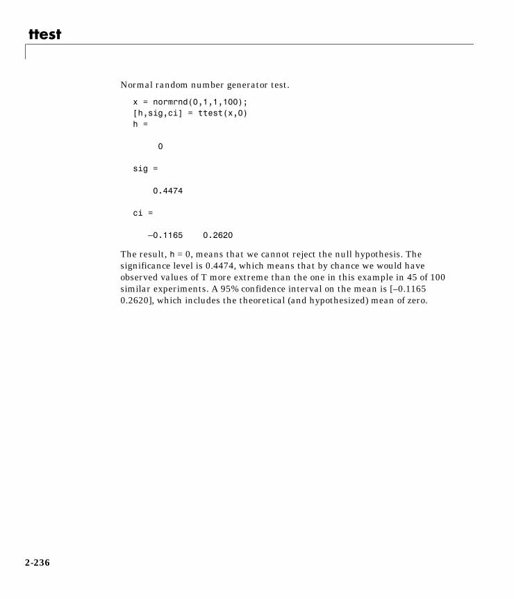
ttest
Normal random number generator test.
x = normrnd(0,1,1,100);[h,sig,ci] = ttest(x,0)h =
0
sig =
0.4474
ci =
–0.1165 0.2620
The result, h = 0, means that we cannot reject the null hypothesis. Thesignificance level is 0.4474, which means that by chance we would haveobserved values of T more extreme than the one in this example in 45 of 100similar experiments. A 95% confidence interval on the mean is [–0.11650.2620], which includes the theoretical (and hypothesized) mean of zero.
2-236
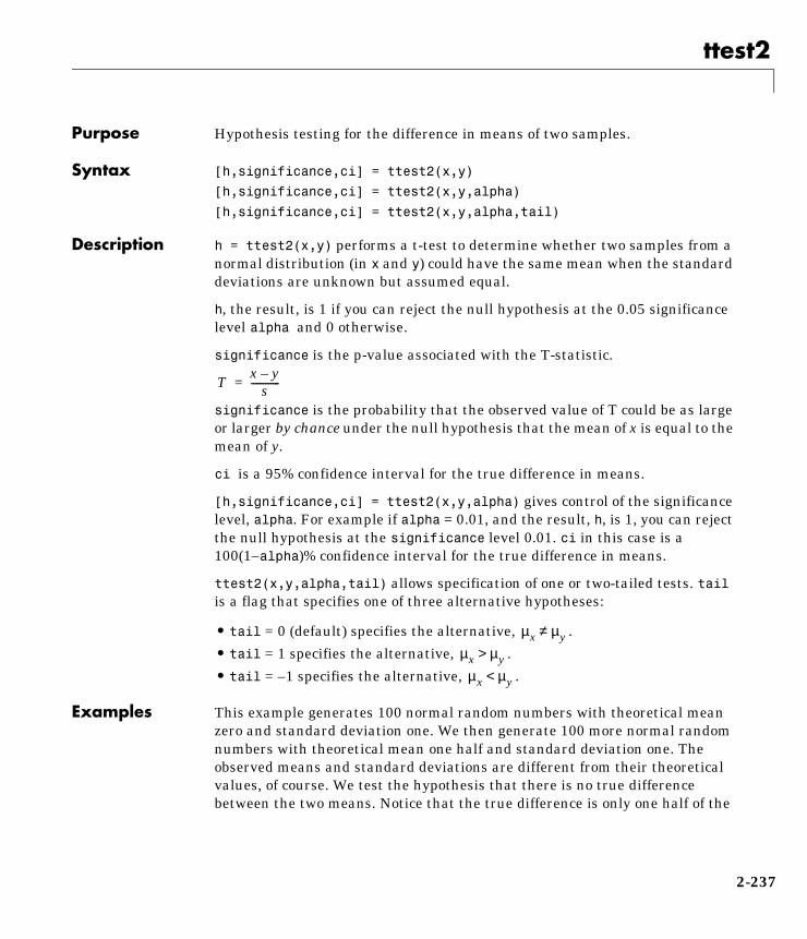
ttest2
2ttest2Purpose Hypothesis testing for the difference in means of two samples.
Syntax [h,significance,ci] = ttest2(x,y)
[h,significance,ci] = ttest2(x,y,alpha)
[h,significance,ci] = ttest2(x,y,alpha,tail)
Description h = ttest2(x,y) performs a t-test to determine whether two samples from anormal distribution (in x and y) could have the same mean when the standarddeviations are unknown but assumed equal.
h, the result, is 1 if you can reject the null hypothesis at the 0.05 significancelevel alpha and 0 otherwise.
significance is the p-value associated with the T-statistic.
significance is the probability that the observed value of T could be as largeor larger by chance under the null hypothesis that the mean of x is equal to themean of y.
ci is a 95% confidence interval for the true difference in means.
[h,significance,ci] = ttest2(x,y,alpha) gives control of the significancelevel, alpha. For example if alpha = 0.01, and the result, h, is 1, you can rejectthe null hypothesis at the significance level 0.01. ci in this case is a100(1–alpha)% confidence interval for the true difference in means.
ttest2(x,y,alpha,tail) allows specification of one or two-tailed tests. tail is a flag that specifies one of three alternative hypotheses:
• tail = 0 (default) specifies the alternative, .
• tail = 1 specifies the alternative, .
• tail = –1 specifies the alternative, .
Examples This example generates 100 normal random numbers with theoretical meanzero and standard deviation one. We then generate 100 more normal randomnumbers with theoretical mean one half and standard deviation one. Theobserved means and standard deviations are different from their theoreticalvalues, of course. We test the hypothesis that there is no true differencebetween the two means. Notice that the true difference is only one half of the
Tx y–
s------------=
µx µy≠µx µy>
µx µy<
2-237
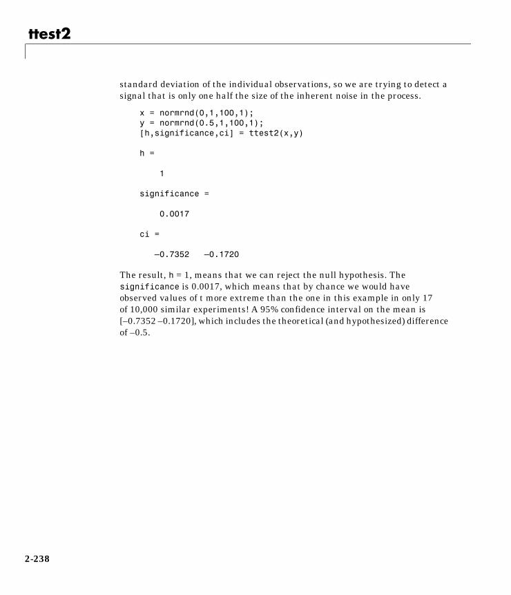
ttest2
standard deviation of the individual observations, so we are trying to detect asignal that is only one half the size of the inherent noise in the process.
x = normrnd(0,1,100,1);y = normrnd(0.5,1,100,1);[h,significance,ci] = ttest2(x,y)
h =
1
significance =
0.0017
ci =
–0.7352 –0.1720
The result, h = 1, means that we can reject the null hypothesis. Thesignificance is 0.0017, which means that by chance we would haveobserved values of t more extreme than the one in this example in only 17of 10,000 similar experiments! A 95% confidence interval on the mean is[–0.7352 –0.1720], which includes the theoretical (and hypothesized) differenceof –0.5.
2-238
unidcdf
2unidcdfPurpose Discrete uniform cumulative distribution (cdf) function.
Syntax P = unidcdf(X,N)
Description unidcdf(X,N) computes the discrete uniform cdf with parameter settings N atthe values in X. The arguments X and N must be the same size except that ascalar argument functions as a constant matrix of the same size of the otherargument.
The maximum observable value, N, is a positive integer.
The discrete uniform cdf is:
The result, p, is the probability that a single observation from the discreteuniform distribution with maximum, N, will be a positive integer less than orequal to x. The values, x, do not need to be integers.
Examples What is the probability of drawing a number 20 or less from a hat with thenumbers from 1 to 50 inside?
probability = unidcdf(20,50)
probability =
0.4000
p F x N( )floor x( )
N----------------------I 1 … N, ,( ) x( )= =
2-239
unidinv
2unidinvPurpose Inverse of the discrete uniform cumulative distribution function.
Syntax X = unidinv(P,N)
Description unidinv(P,N) returns the smallest integer X such that the discrete uniform cdfevaluated at X is equal to or exceeds P. You can think of P as the probability ofdrawing a number as large as X out of a hat with the numbers 1 through Ninside.
The argument P must lie on the interval [0 1] and N must be a positive integer.Each element of X is a positive integer.
Examples x = unidinv(0.7,20)
x =
14
y = unidinv(0.7 + eps,20)
y =
15
A small change in the first parameter produces a large jump in output. The cdfand its inverse are both step functions. The example shows what happens at astep.
2-240
unidpdf
2unidpdfPurpose Discrete uniform probability density function (pdf).
Syntax Y = unidpdf(X,N)
Description unidpdf(X,N) computes the discrete uniform pdf with parameter settings, N, atthe values in X. The arguments X and N must be the same size except that ascalar argument functions as a constant matrix of the same size of the otherargument.
The parameter N must be a positive integer.
The discrete uniform pdf is:
You can think of y as the probability of observing any one number between 1and n.
Examples For fixed n, the uniform discrete pdf is a constant.
y = unidpdf(1:6,10)
y =
0.1000 0.1000 0.1000 0.1000 0.1000 0.1000
Now fix x , and vary n.
likelihood = unidpdf(5,4:9)
likelihood =
0 0.2000 0.1667 0.1429 0.1250 0.1111
y f x N( )1N----I 1 … N, ,( ) x( )= =
2-241
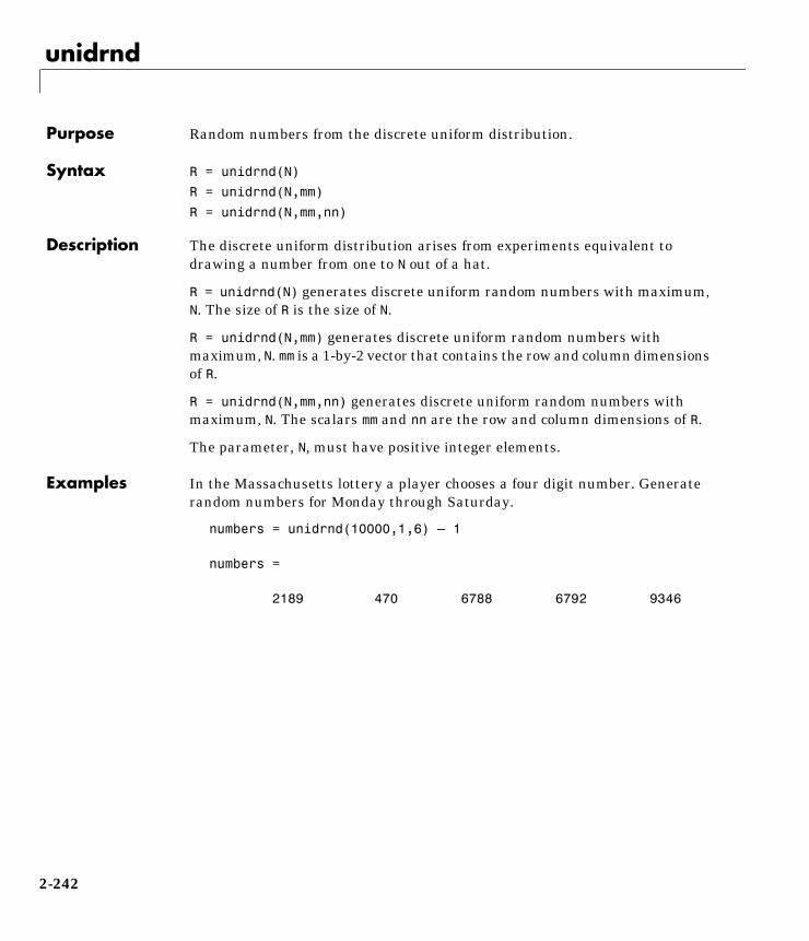
unidrnd
2unidrndPurpose Random numbers from the discrete uniform distribution.
Syntax R = unidrnd(N)
R = unidrnd(N,mm)
R = unidrnd(N,mm,nn)
Description The discrete uniform distribution arises from experiments equivalent todrawing a number from one to N out of a hat.
R = unidrnd(N) generates discrete uniform random numbers with maximum,N. The size of R is the size of N.
R = unidrnd(N,mm) generates discrete uniform random numbers withmaximum, N. mm is a 1-by-2 vector that contains the row and column dimensionsof R.
R = unidrnd(N,mm,nn) generates discrete uniform random numbers withmaximum, N. The scalars mm and nn are the row and column dimensions of R.
The parameter, N, must have positive integer elements.
Examples In the Massachusetts lottery a player chooses a four digit number. Generaterandom numbers for Monday through Saturday.
numbers = unidrnd(10000,1,6) – 1
numbers =
2189 470 6788 6792 9346
2-242
unidstat
2unidstatPurpose Mean and variance for the discrete uniform distribution.
Syntax [M,V] = unidstat(N)
Description For the discrete uniform distribution:
• The mean is .
• The variance is .
Examples [m,v] = unidstat(1:6)
m =
1.0000 1.5000 2.0000 2.5000 3.0000 3.5000
v =
0 0.2500 0.6667 1.2500 2.0000 2.9167
N 1+2--------------
N2 1–12-----------------
2-243
unifcdf
2unifcdfPurpose Continuous uniform cumulative distribution function (cdf).
Syntax P = unifcdf(X,A,B)
Description unifcdf(X,A,B) computes the uniform cdf with parameters A and B at thevalues in X. The arguments X, A and B must all be the same size except thatscalar arguments function as constant matrices of the common size of the otherarguments.
A and B are the minimum and maximum values respectively.
The uniform cdf is:
The standard uniform distribution has A = 0 and B = 1.
Examples What is the probability that an observation from a standard uniformdistribution will be less than 0.75?
probability = unifcdf(0.75)
probability =
0.7500
What is the probability that an observation from a uniform distribution witha = –1 and b = 1 will be less than 0.75?
probability = unifcdf(0.75,–1,1)
probability =
0.8750
p F x a b,( )x a–b a–------------I a b,[ ] x( )= =
2-244
unifinv
2unifinvPurpose Inverse continuous uniform cumulative distribution function (cdf).
Syntax X = unifinv(P,A,B)
Description unifinv(P,A,B) computes the inverse of the uniform cdf with parameters Aand B at the values in X. The arguments X, A, and B must all be the same sizeexcept that scalar arguments function as constant matrices of the common sizeof the other arguments.
A and B are the minimum and maximum values respectively.
The inverse of the uniform cdf is:
The standard uniform distribution has A = 0 and B = 1.
Examples What is the median of the standard uniform distribution?
median_value = unifinv(0.5)
median_value =
0.5000
What is the 99th percentile of the uniform distribution between –1 and 1?
percentile = unifinv(0.99,–1,1)
percentile =
0.9800
x F 1– p a b,( ) a p a b–( )I 0 1,[ ] p( )+= =
2-245
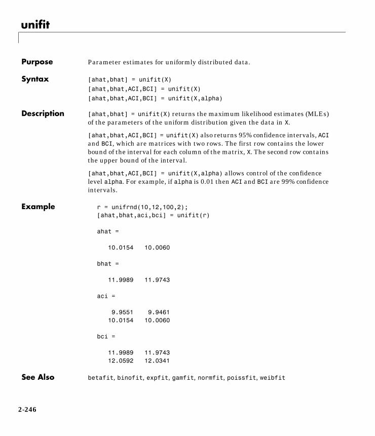
unifit
2unifitPurpose Parameter estimates for uniformly distributed data.
Syntax [ahat,bhat] = unifit(X)
[ahat,bhat,ACI,BCI] = unifit(X)
[ahat,bhat,ACI,BCI] = unifit(X,alpha)
Description [ahat,bhat] = unifit(X) returns the maximum likelihood estimates (MLEs)of the parameters of the uniform distribution given the data in X.
[ahat,bhat,ACI,BCI] = unifit(X) also returns 95% confidence intervals, ACIand BCI, which are matrices with two rows. The first row contains the lowerbound of the interval for each column of the matrix, X. The second row containsthe upper bound of the interval.
[ahat,bhat,ACI,BCI] = unifit(X,alpha) allows control of the confidencelevel alpha. For example, if alpha is 0.01 then ACI and BCI are 99% confidenceintervals.
Example r = unifrnd(10,12,100,2);[ahat,bhat,aci,bci] = unifit(r)
ahat =
10.0154 10.0060
bhat =
11.9989 11.9743
aci =
9.9551 9.9461 10.0154 10.0060
bci =
11.9989 11.9743 12.0592 12.0341
See Also betafit, binofit, expfit, gamfit, normfit, poissfit, weibfit
2-246

unifpdf
2unifpdfPurpose Continuous uniform probability density function (pdf).
Syntax Y = unifpdf(X,A,B)
Description unifpdf(X,A,B) computes the continuous uniform pdf with parameters A andB at the values in X. The arguments X, A, and B must all be the same size exceptthat scalar arguments function as constant matrices of the common size of theother arguments.
The parameter B must be greater than A.
The continuous uniform distribution pdf is:
The standard uniform distribution has A = 0 and B = 1.
Examples For fixed a and b, the uniform pdf is constant.
x = 0.1:0.1:0.6;y = unifpdf(x)
y =
1 1 1 1 1 1
What if x is not between a and b?
y = unifpdf(–1,0,1)
y =
0
y f x a b,( )1
b a–------------I a b,[ ] x( )= =
2-247

unifrnd
2unifrndPurpose Random numbers from the continuous uniform distribution.
Syntax R = unifrnd(A,B)
R = unifrnd(A,B,m)
R = unifrnd(A,B,m,n)
Description R = unifrnd(A,B) generates uniform random numbers with parameters A andB. The size of R is the common size of A and B if both are matrices. If eitherparameter is a scalar, the size of R is the size of the other parameter.
R = unifrnd(A,B,m) generates uniform random numbers with parameters Aand B. m is a 1-by-2 vector that contains the row and column dimensions of R.
R = unifrnd(A,B,m,n) generates uniform random numbers with parametersA and B. The scalars m and n are the row and column dimensions of R.
Examples random = unifrnd(0,1:6)
random =
0.2190 0.0941 2.0366 2.7172 4.6735 2.3010
random = unifrnd(0,1:6,[1 6])
random =
0.5194 1.6619 0.1037 0.2138 2.6485 4.0269
random = unifrnd(0,1,2,3)
random =
0.0077 0.0668 0.6868 0.3834 0.4175 0.5890
2-248
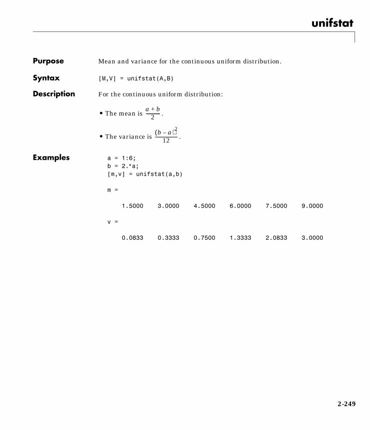
unifstat
2unifstatPurpose Mean and variance for the continuous uniform distribution.
Syntax [M,V] = unifstat(A,B)
Description For the continuous uniform distribution:
• The mean is .
• The variance is .
Examples a = 1:6;b = 2.∗a;[m,v] = unifstat(a,b)
m =
1.5000 3.0000 4.5000 6.0000 7.5000 9.0000
v =
0.0833 0.3333 0.7500 1.3333 2.0833 3.0000
a b+2-------------
b a–( )2
12--------------------
2-249

var
2varPurpose Variance of a sample.
Syntax y = var(X)y = var(X,1)y = var(X,w)
Description var(X) computes the variance of the data in X. For vectors, var(x) is thevariance of the elements in x. For matrices, var(X) is a row vector containingthe variance of each column of X.
var(x) normalizes by n–1 where n is the sequence length. For normallydistributed data, this makes var(x) the minimum variance unbiased estimatorMVUE of σ 2(the second parameter) .
var(x,1) normalizes by n and yields the second moment of the sample dataabout its mean (moment of inertia).
var(X,w) computes the variance using the vector of weights, w. The number ofelements in w must equal the number of rows in the matrix, X. For vector x, wand x must match in length. Each element of w must be positive.
var supports both common definitions of variance. Let SS be the sum ofthe squared deviations of the elements of a vector x, from their mean. Then,var(x) = SS/(n-1) the MVUE, and var(x,1) = SS/n the maximum likelihoodestimator (MLE) of σ 2.
2-250
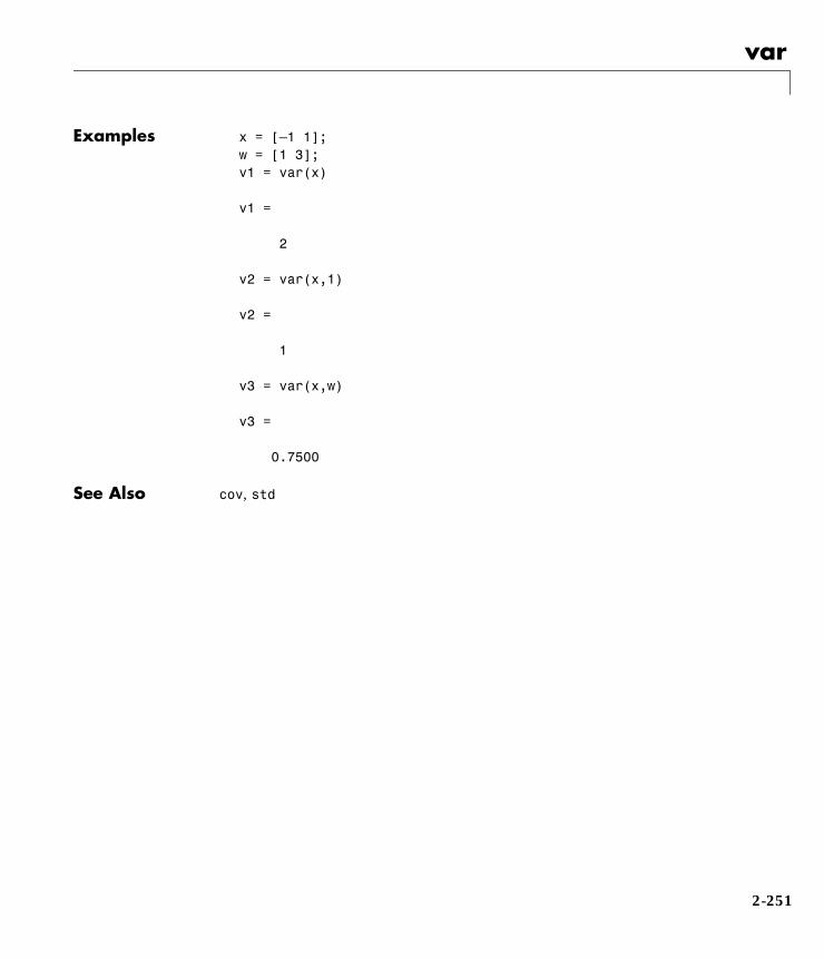
var
Examples x = [–1 1];w = [1 3];v1 = var(x)
v1 =
2
v2 = var(x,1)
v2 =
1
v3 = var(x,w)
v3 =
0.7500
See Also cov, std
2-251
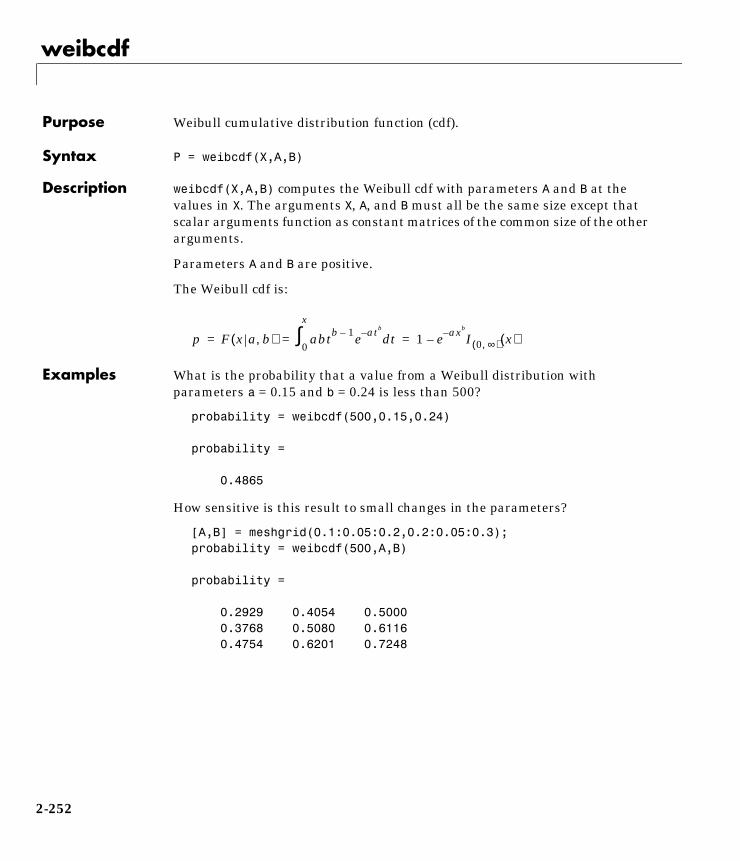
weibcdf
2weibcdfPurpose Weibull cumulative distribution function (cdf).
Syntax P = weibcdf(X,A,B)
Description weibcdf(X,A,B) computes the Weibull cdf with parameters A and B at thevalues in X. The arguments X, A, and B must all be the same size except thatscalar arguments function as constant matrices of the common size of the otherarguments.
Parameters A and B are positive.
The Weibull cdf is:
Examples What is the probability that a value from a Weibull distribution withparameters a = 0.15 and b = 0.24 is less than 500?
probability = weibcdf(500,0.15,0.24)
probability =
0.4865
How sensitive is this result to small changes in the parameters?
[A,B] = meshgrid(0.1:0.05:0.2,0.2:0.05:0.3);probability = weibcdf(500,A,B)
probability =
0.2929 0.4054 0.5000 0.3768 0.5080 0.6116 0.4754 0.6201 0.7248
p F x a b,( ) abtb 1– e atb– td0
x
∫ 1 e axb– I 0 ∞,( ) x( )–= = =
2-252
weibfit
2weibfitPurpose Parameter estimates and confidence intervals for Weibull data.
Syntax phat = weibfit(x)
[phat,pci] = weibfit(x)
[phat,pci] = weibfit(x,alpha)
Description phat = weibfit(x) returns the maximum likelihood estimates, phat, of theparameters of the Weibull distribution given the data in the vector, x. phat isa two-element row vector. phat(1) estimates the Weibull parameter, a, andphat(2) estimates b in the pdf:
[phat,pci] = weibfit(x) also returns 95% confidence intervals in a matrix,pci, with 2 rows. The first row contains the lower bound of the confidenceinterval. The second row contains the upper bound. The columns of pcicorrespond to the columns of phat.
[phat,pci] = weibfit(x,alpha) allows control over the confidence intervalreturned (100(1–alpha)%).
Example r = weibrnd(0.5,0.8,100,1);[phat,pci] = weibfit(r)
phat =
0.4746 0.7832
pci =
0.3851 0.6367 0.5641 0.9298
See Also betafit, binofit, expfit, gamfit, normfit, poissfit, unifit
y f x a b,( ) abxb 1– e axb– I 0 ∞,( ) x( )= =
2-253
weibinv
2weibinvPurpose Inverse of the Weibull cumulative distribution function.
Syntax X = weibinv(P,A,B)
Description weibinv(P,A,B) computes the inverse of the Weibull cdf with parameters Aand B for the probabilities in P. The arguments P, A and B must all be the samesize except that scalar arguments function as constant matrices of the commonsize of the other arguments.
The parameters A and B must be positive.
The inverse of the Weibull cdf is:
Examples A batch of light bulbs have lifetimes (in hours) distributed Weibull withparameters a = 0.15 and b = 0.24. What is the median lifetime of the bulbs?
life = weibinv(0.5,0.15,0.24)
life =
588.4721
What is the 90th percentile?
life = weibinv(0.9,0.15,0.24)
life =
8.7536e+04
x F 1– p a b,( )1a---
11 p–------------
ln
1b---
I 0 1,[ ] p( )= =
2-254
weiblike
2weiblikePurpose Weibull negative log-likelihood function.
Syntax logL = weiblike(params,data)
[logL,info] = weiblike(params,data)
Description logL = weiblike(params,data) returns the Weibull log-likelihood withparameters params(1) = a and params(2) = b given the data, xi.
[logL,info] = weiblike(params,data) adds Fisher's information matrix,info. The diagonal elements of INFO are the asymptotic variances of theirrespective parameters.
The Weibull negative log-likelihood is:
weiblike is a utility function for maximum likelihood estimation.
Example Continuing the example for weibfit:
r = weibrnd(0.5,0.8,100,1);[logL,info] = weiblike([0.4746 0.7832],r)
logL =
203.8216
info =
0.0021 0.0022 0.0022 0.0056
Reference Patel, J. K., C. H. Kapadia, and D. B. Owen, Handbook of StatisticalDistributions, Marcel-Dekker, 1976.
See Also betalike, gamlike, mle, weibfit
Llog– f a b, xi( )i 1=
∏log– f a b, xi( )log
i 1=
n
∑–= =
2-255

weibpdf
2weibpdfPurpose Weibull probability density function (pdf).
Syntax Y = weibpdf(X,A,B)
Description weibpdf(X,A,B) computes the Weibull pdf with parameters A and B at thevalues in X. The arguments X, A and B must all be the same size except thatscalar arguments function as constant matrices of the common size of the otherarguments.
Parameters A and B are positive.
The Weibull pdf is:
Some references refer to the Weibull distribution with a single parameter. Thiscorresponds to weibpdf with A =1.
Examples The exponential distribution is a special case of the Weibull distribution.
lambda = 1:6;y = weibpdf(0.1:0.1:0.6,lambda,1)
y =
0.9048 1.3406 1.2197 0.8076 0.4104 0.1639
y1 = exppdf(0.1:0.1:0.6,1./lambda)
y1 =
0.9048 1.3406 1.2197 0.8076 0.4104 0.1639
Reference Devroye, L., Non-Uniform Random Variate Generation. Springer-Verlag. NewYork, 1986.
y f x a b,( ) abxb 1– e axb– I 0 ∞,( ) x( )= =
2-256
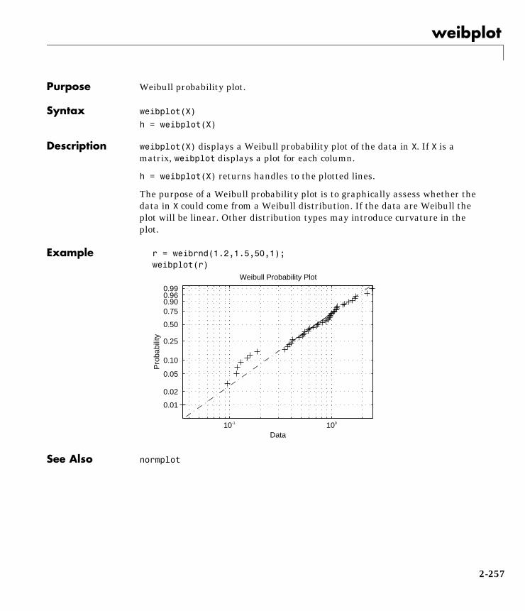
weibplot
2weibplotPurpose Weibull probability plot.
Syntax weibplot(X)
h = weibplot(X)
Description weibplot(X) displays a Weibull probability plot of the data in X. If X is amatrix, weibplot displays a plot for each column.
h = weibplot(X) returns handles to the plotted lines.
The purpose of a Weibull probability plot is to graphically assess whether thedata in X could come from a Weibull distribution. If the data are Weibull theplot will be linear. Other distribution types may introduce curvature in theplot.
Example r = weibrnd(1.2,1.5,50,1);weibplot(r)
See Also normplot
10-1 100
0.01
0.02
0.05
0.10
0.25
0.50
0.75 0.90 0.96 0.99
Data
Pro
babi
lity
Weibull Probability Plot
2-257
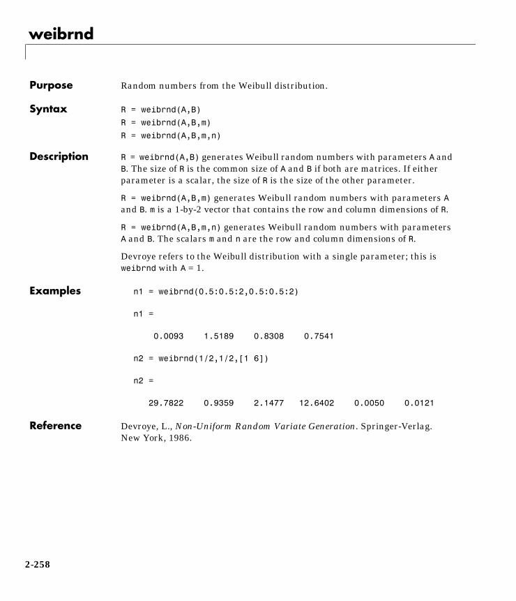
weibrnd
2weibrndPurpose Random numbers from the Weibull distribution.
Syntax R = weibrnd(A,B)
R = weibrnd(A,B,m)
R = weibrnd(A,B,m,n)
Description R = weibrnd(A,B) generates Weibull random numbers with parameters A andB. The size of R is the common size of A and B if both are matrices. If eitherparameter is a scalar, the size of R is the size of the other parameter.
R = weibrnd(A,B,m) generates Weibull random numbers with parameters Aand B. m is a 1-by-2 vector that contains the row and column dimensions of R.
R = weibrnd(A,B,m,n) generates Weibull random numbers with parametersA and B. The scalars m and n are the row and column dimensions of R.
Devroye refers to the Weibull distribution with a single parameter; this isweibrnd with A = 1.
Examples n1 = weibrnd(0.5:0.5:2,0.5:0.5:2)
n1 =
0.0093 1.5189 0.8308 0.7541
n2 = weibrnd(1/2,1/2,[1 6])
n2 =
29.7822 0.9359 2.1477 12.6402 0.0050 0.0121
Reference Devroye, L., Non-Uniform Random Variate Generation. Springer-Verlag.New York, 1986.
2-258

weibstat
2weibstatPurpose Mean and variance for the Weibull distribution.
Syntax [M,V] = weibstat(A,B)
Description For the Weibull distribution:
• The mean is:
• The variance is:
Examples [m,v] = weibstat(1:4,1:4)
m =
1.0000 0.6267 0.6192 0.6409
v =
1.0000 0.1073 0.0506 0.0323
weibstat(0.5,0.7)
ans =
3.4073
a
1b---–
Γ 1 b 1–+( )
a
2b---–
Γ 1 2b 1–+( ) Γ2 1 b 1–
+( )–
2-259
x2fx
2x2fxPurpose Transform a factor settings matrix to a design matrix.
Syntax D = x2fx(X)
D = x2fx(X,'model')
Description D = x2fx(X) transforms a matrix of system inputs, X, to a design matrix for alinear additive model with a constant term.
D = x2fx(X,'model') allows control of the order of the regressionmodel.'model' can be one of these strings:
• 'interaction' – includes constant, linear, and cross product terms.
• 'quadratic' – interactions plus squared terms.
• 'purequadratic' – includes constant, linear and squared terms.
Alternatively, the argument, model, can be a matrix of terms. In this case eachrow of model represents one term. The value in a column is the exponent toraise the same column in X for that term. This allows for models withpolynomial terms of arbitrary order.
x2fx is a utility function for rstool, regstats and cordexch.
Example x = [1 2 3;4 5 6]'; model = 'quadratic';D = x2fx(x,model)
D =
1 1 4 4 1 16 1 2 5 10 4 25 1 3 6 18 9 36
Let x1 be the first column of x and x2 be the second. Then, the first column of Dis for the constant term. The second column is x1 . The 3rd column is x2. The 4this x1x2. The fifth is x1
2 and the last is x22.
See Also rstool, cordexch, rowexch, regstats
2-260
xbarplot
2xbarplotPurpose X-bar chart for Statistical Process Control.
Syntax xbarplot(DATA)
xbarplot(DATA,conf)
xbarplot(DATA,conf,specs)
[outlier,h] = xbarplot(...)
Description xbarplot(DATA) displays an x-bar chart of the grouped responses in DATA. Therows of DATA contain replicate observations taken at a given time. The rowsmust be in time order. The upper and lower control limits are a 99% confidenceinterval on a new observation from the process. So, roughly 99% of the plottedpoints should fall between the control limits.
xbarplot(DATA,conf) allows control of the the confidence level of the upperand lower plotted confidence limits. For example, conf = 0.95 plots 95%confidence intervals.
xbarplot(DATA,conf,specs) plots the specification limits in the two elementvector, specs.
[outlier,h] = xbarplot(DATA,conf,specs) returns outlier, a vector ofindices to the rows where the mean of DATA is out of control, and h, a vector ofhandles to the plotted lines.
Example Plot an x-bar chart of measurements on newly machined parts, taken at onehour intervals for 36 hours. Each row of the runout matrix contains themeasurements for four parts chosen at random. The values indicate, in
2-261
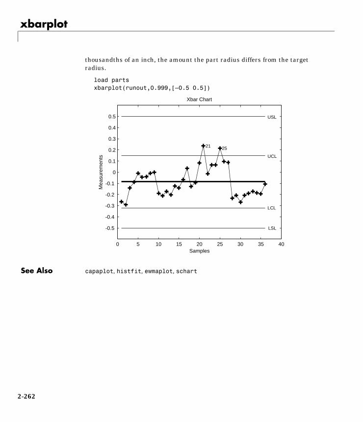
xbarplot
thousandths of an inch, the amount the part radius differs from the targetradius.
load partsxbarplot(runout,0.999,[–0.5 0.5])
See Also capaplot, histfit, ewmaplot, schart
0 5 10 15 20 25 30 35 40
-0.5
-0.4
-0.3
-0.2
-0.1
0
0.1
0.2
0.3
0.4
0.5
21 25
Xbar Chart
Samples
Mea
sure
men
ts
LCL
UCL
USL
LSL
2-262

zscore
2zscore
Purpose Standardized Z score.
Syntax Z = zscore(D)
Description Z = zscore(D) returns the deviation of each column of D from its mean,normalized by its standard deviation. This is known as the Z score of D.
For column vector V, Z score is Z = (V-mean(V))./std(V)
2-263

ztest
2ztestPurpose Hypothesis testing for the mean of one sample with known variance.
Syntax h = ztest(x,m,sigma)
h = ztest(x,m,sigma,alpha)
[h,sig,ci] = ztest(x,m,sigma,alpha,tail)
Description ztest(x,m,sigma) performs a Z test at significance level 0.05 to determinewhether a sample from a normal distribution (in x) could have mean m andstandard deviation, sigma.
h = ztest(x,m,sigma,alpha) gives control of the significance level, alpha. Forexample if alpha = 0.01, and the result, h, is 1 you can reject the null hypothesisat the significance level 0.01. If h = 0, you cannot reject the null hypothesis atthe alpha level of significance.
[h,sig,ci] = ztest(x,m,sigma,alpha,tail) allows specification of one ortwo-tailed tests. tail is a flag that specifies one of three alternativehypotheses:
• tail = 0 (default) specifies the alternative, .
• tail = 1 specifies the alternative, .
• tail = –1 specifies the alternative, .
sig is the p-value associated with the Z statistic.
sig is the probability that the observed value of Z could be as large or larger bychance under the null hypothesis that the mean of x is equal to µ.
ci is a 1–alpha confidence interval for the true mean.
Example This example generates 100 normal random numbers with theoretical meanzero and standard deviation one. The observed mean and standard deviation
x µ≠x µ>
x µ<
zx µ–
σ------------=
2-264

ztest
are different from their theoretical values, of course. We test the hypothesisthat there is no true difference.
x = normrnd(0,1,100,1);m = mean(x)m =
0.0727
[h,sig,ci] = ztest(x,0,1)
h =
0
sig =
0.4669
ci =
–0.1232 0.2687
The result, h = 0, means that we cannot reject the null hypothesis. Thesignificance level is 0.4669, which means that by chance we would haveobserved values of Z more extreme than the one in this example in 47 of 100similar experiments. A 95% confidence interval on the mean is [–0.12320.2687], which includes the theoretical (and hypothesized) mean of zero.
2-265

ztest
2-266

Index
Aabsolute deviation 1-44additive 1-67alternative hypothesis 1-85analysis of variance 1-24ANOVA 1-65anova1 2-12, 2-16anova2 2-12, 2-20average linkage 2-121
Bbacteria counts 1-65barttest 2-13baseball odds 2-31, 2-33Bernoulli random variables 2-35beta distribution 1-12, 1-13betacdf 2-3, 2-24betafit 2-3, 2-25betainv 2-5, 2-26betalike 2-3, 2-27betapdf 2-4, 2-28betarnd 2-6, 2-29betastat 2-8, 2-30binocdf 2-3, 2-31binofit 2-3, 2-32binoinv 2-5, 2-33binomial distribution 1-12, 1-15binopdf 2-4, 2-34binornd 2-6, 2-35binostat 2-8, 2-36bootstrap 2-37bootstrap sampling 1-47box plots 1-103boxplot 2-10, 2-39
Ccapability studies 1-113capable 2-11, 2-41capaplot 2-11caseread 2-14, 2-44casewrite 2-14, 2-45cdf 1-6, 1-7cdf 2-3, 2-46census 2-14Central Limit Theorem 1-31centroid linkage 2-121Chatterjee and Hadi example 1-72chi2cdf 2-3, 2-47chi2inv 2-5, 2-48chi2pdf 2-4, 2-49chi2rnd 2-6, 2-50chi2stat 2-8, 2-51chi-square distribution 1-12, 1-17circuit boards 2-34cities 2-14City Block metric
in cluster analysis 2-179classify 2-52cluster 2-11, 2-53cluster analysis 1-50
computing inconsistency coefficient 1-57,2-115
creating clusters from data 2-55creating clusters from linkage output 1-61,
2-53creating the cluster tree 1-53, 2-120determining proximity 1-51, 2-178evaluating cluster formation 1-56, 2-58formatting distance information 1-53, 2-221overview 1-50plotting the cluster tree 1-55, 2-65
I-1
Index
I-2
clusterdata 2-11, 2-55coin 2-95combnk 2-57complete linkage 2-121confidence intervals
hypothesis tests 1-86nonlinear regression 1-82
control charts 1-110EWMA charts 1-112S charts 1-111Xbar charts 1-110
cophenet 2-11, 2-58using 1-56
cophenetic correlation coefficient 2-58defined 1-56
cordexch 2-13, 2-59corrcoef 2-60cov 2-61Cp index 1-114, 2-41Cpk index 1-114, 2-41crosstab 2-62cumulative distribution function (cdf) 1-6
Ddata 2-2daugment 2-13, 2-63dcovary 2-13, 2-64demos 1-125, 2-2
design of experiments 1-131polynomial curve fitting 1-126probability distributions 1-125random number generation 1-130
dendrogram 2-11, 2-65using 1-55
depthin cluster analysis 1-59
descriptive 2-2descriptive statistics 1-42Design of Experiments 1-115
D-optimal designs 1-118fractional factorial designs 1-117full factorial designs 1-116
discrete uniform distribution 1-12, 1-20discrim 2-14dissimilarity matrix
creating 1-51distributions 1-2, 1-5disttool 2-14, 2-68DOE. See Design of ExperimentsD-optimal designs 1-118dummyvar 2-69
Eerf 1-31error function 1-31errorbar 2-10, 2-70estimate 1-128Euclidean distance
in cluster analysis 2-179EWMA charts 1-112ewmaplot 2-11, 2-71expcdf 2-3, 2-73expfit 2-3, 2-74expinv 2-5, 2-75exponential distribution 1-12, 1-21exppdf 2-4, 2-76exprnd 2-6, 2-77expstat 2-8, 2-78extrapolated 2-194
Index
FF distribution 1-12, 1-23F statistic 1-72fcdf 2-3, 2-79ff2n 2-13, 2-80file i/o 2-2finv 2-5, 2-81floppy disks 2-109fpdf 2-4, 2-82fractional factorial designs 1-117frnd 2-6, 2-83fstat 2-8, 2-84fsurfht 2-10, 2-85full factorial designs 1-116fullfact 2-13, 2-87furthest neighbor linkage 2-121
Ggamcdf 2-3, 2-88gamfit 2-3, 2-89gaminv 2-5, 2-90gamlike 2-3, 2-91gamma distribution 1-12, 1-25gampdf 2-4, 2-92gamrnd 2-6, 2-93gamstat 2-8, 2-94gas 2-14Gaussian 2-106geocdf 2-3, 2-95geoinv 2-5, 2-96geomean 2-9, 2-97geometric distribution 1-12, 1-27geopdf 2-4, 2-98geornd 2-7, 2-99geostat 2-8, 2-100gline 2-10, 2-101
gname 2-10, 2-102grpstats 2-104Guinness beer 1-36, 2-229
Hhadamard 2-13hald 2-14harmmean 2-9, 2-105hat matrix 1-70hist 2-106histfit 2-11, 2-107histogram 1-130hogg 2-14Hotelling’s T squared 1-102hougen 2-108Hougen-Watson model 1-79hygecdf 2-3, 2-109hygeinv 2-6, 2-110hygepdf 2-4, 2-111hygernd 2-7, 2-112hygestat 2-8, 2-113hypergeometric distribution 1-12, 1-28hypotheses 1-24, 2-2hypothesis tests 1-85
Iicdf 2-114incomplete beta function 1-13incomplete gamma function 1-25inconsistency coefficient 1-58inconsistent 2-11, 2-115
using 1-58inspector 2-182integral equation 2-26interaction 1-67
I-3
Index
I-4
interpolated 2-224interquartile range (iqr) 1-44inverse cdf 1-6, 1-7iqr 2-9, 2-117
Kkurtosis 2-9, 2-118
Llawdata 2-14least-squares 2-189leverage 2-119light bulbs, life of 2-75likelihood function 2-28linear 2-2linear models 1-65linkage 2-11, 2-120
using 1-53logncdf 2-4, 2-123logninv 2-6, 2-124lognormal distribution 1-13, 1-29lognpdf 2-5, 2-125lognrnd 2-7, 2-126lognstat 2-8, 2-127lottery 2-242lsline 2-10, 2-128LU factorizations 2-188
Mmad 2-9, 2-129mahal 2-130Mahalanobis distance 2-130
in cluster analysis 2-179mean 1-6, 1-11
mean 2-9, 2-131Mean Squares (MS) 2-16measures of central tendency 1-42measures of dispersion 1-43median 2-9, 2-132mileage 2-14Minkowski metric
in cluster analysis 2-179mle 2-3, 2-133models
linear 1-65nonlinear 1-79
moment 2-9, 2-134Monte Carlo simulation 2-117moore 2-15multiple linear regression 1-69multivariate statistics 1-91mvnrnd 2-135
Nnanmax 2-9, 2-136nanmean 2-9, 2-137nanmedian 2-9, 2-138nanmin 2-9, 2-139NaNs 1-45nanstd 2-9, 2-140nansum 2-9, 2-141nbincdf 2-4, 2-142nbininv 2-6, 2-143nbinpdf 2-5, 2-144nbinrnd 2-7, 2-145nbinstat 2-8, 2-146ncfcdf 2-4, 2-147ncfinv 2-6, 2-148ncfpdf 2-5, 2-149ncfrnd 2-7, 2-150
Index
ncfstat 2-8, 2-151nctcdf 2-4, 2-152nctinv 2-6, 2-153nctpdf 2-5, 2-154nctrnd 2-7, 2-155nctstat 2-8, 2-156ncx2cdf 2-4, 2-157ncx2inv 2-6, 2-158ncx2pdf 2-5, 2-159ncx2rnd 2-7, 2-160ncx2stat 2-8, 2-161nearest neighbor linkage 2-121negative binomial distribution 1-13, 1-30Newton’s method 2-90nlinfit 2-12, 2-162nlintool 2-12, 2-163nlparci 2-12, 2-164nlpredci 2-12, 2-165noncentral chi-square distribution 1-12noncentral F distribution 1-12, 1-24noncentral t distribution 1-13, 1-37nonlinear 2-2nonlinear regression models 1-79normal distribution 1-13, 1-31normal probability plots 1-103, 1-104normalizing a dataset 1-51
using zscore 2-263normcdf 2-4, 2-166normdemo 2-11, 2-172normfit 2-3, 2-167norminv 2-6, 2-168normlike 2-3normpdf 2-5, 2-169normplot 2-10, 2-170normrnd 2-7, 2-171normstat 2-8, 2-173notches 2-39
null 1-85null hypothesis 1-85
Oone-way analysis of variance (ANOVA) 1-65outliers 1-42
Ppareto 2-10, 2-174parts 2-15Pascal, Blaise 1-15PCA. See Principal Components Analysispcacov 2-13, 2-175pcares 2-13, 2-176pdf 1-6pdf 2-177pdist 2-11, 2-178
using 1-51percentiles 1-46perms 2-181plots 1-46, 2-2poisscdf 2-4, 2-182poissfit 2-3, 2-183poissinv 2-6, 2-184Poisson distribution 1-13, 1-33poisspdf 2-5, 2-185poissrnd 2-7, 2-186poisstat 2-8, 2-187polyconf 2-12, 2-188polydata 2-15polyfit 2-12, 2-189polynomial 1-126polytool 1-125, 2-14, 2-190polyval 2-12, 2-191popcorn 2-21
I-5

Index
I-6
popcorn 2-15prctile 2-9, 2-192Principal Components Analysis 1-91
component scores 1-95component variances 1-99Hotelling’s T squared 1-102Scree plot 1-101
princomp 2-13, 2-193probability 2-2probability density function (pdf) 1-6probability distributions 1-5p-value 1-69, 1-86
Qqqplot 2-10, 2-194QR decomposition 1-70quality assurance 2-34quantile-quantile plots 1-103, 1-106
Rrandom 2-195random number generator 1-6random numbers 1-9randtool 1-125, 2-14, 2-68, 2-196range 2-9, 2-197ranksum 2-13, 2-198raylcdf 2-4, 2-199Rayleigh distribution 1-13raylinv 2-6, 2-200raylpdf 2-5, 2-201raylrnd 2-7, 2-202raylstat 2-8, 2-203rcoplot 2-10, 2-204reaction 2-15refcurve 2-10, 2-205
reference lines 1-125references 1-134refline 2-10, 2-206regress 2-12, 2-207regression 1-24
nonlinear 1-79stepwise 1-75
regstats 2-209relative efficiency 2-117residuals 1-73Response Surface Methodology (RSM) 1-73ridge 2-12, 2-211robust 1-42robust linear fit 2-194rowexch 2-13, 2-213rsmdemo 1-125, 2-14, 2-214R-square 1-72rstool 2-12, 2-215
SS charts 1-111sat 2-15schart 2-11, 2-216Scree plot 1-101segmentation analysis 1-50significance level 1-85signrank 2-13, 2-218signtest 2-13, 2-219similarity matrix
creating 1-51simulation 2-117single linkage 2-121skewness 1-103skewness 2-9, 2-220SPC. See Statistical Process Controlsquareform 2-11, 2-221
Index
standard normal 2-169Standardized Euclidean distance
in cluster analysis 2-179statdemo 2-14, 2-221statistical plots 1-103Statistical Process Control
capability studies 1-113control charts 1-110
statistical references 1-134statistically significant 2-16std 2-9, 2-221stepwise 2-12, 2-223stepwise regression 1-75Sum of Squares (SS) 2-16surfht 2-10, 2-224symmetric 2-88
Tt distribution 1-13, 1-36tabulate 2-225taxonomy analysis 1-50tblread 2-14, 2-226tblwrite 2-14, 2-228tcdf 2-4, 2-229tinv 2-6, 2-230tpdf 2-5, 2-231trimmean 2-9, 2-232trnd 2-7, 2-233tstat 2-8, 2-234ttest 2-13, 2-235ttest2 2-13, 2-237two-way ANOVA 1-67
Uunbiased 2-222, 2-250
unidcdf 2-4, 2-239unidinv 2-6, 2-240unidpdf 2-5, 2-241unidrnd 2-7, 2-242unidstat 2-8, 2-243unifcdf 2-4, 2-244unifinv 2-6, 2-245unifit 2-3, 2-246uniform distribution 1-13, 1-38unifpdf 2-5, 2-247unifrnd 2-7, 2-248unifstat 2-8, 2-249
Vvar 2-9, 2-250variance 1-6, 1-11
Wward linkage 2-122weibcdf 2-4, 2-252weibfit 2-253weibinv 2-6, 2-254weiblike 2-255weibpdf 2-5, 2-256weibplot 2-10, 2-257weibrnd 2-7, 2-258weibstat 2-8, 2-259Weibull distribution 1-13, 1-39Weibull probability plots 1-108Weibull, Waloddi 1-39whiskers 1-103, 2-39
Xx2fx 2-260
I-7

Index
I-8
Xbar charts 1-110xbarplot 2-11, 2-261
Zzscore 2-263ztest 2-13, 2-264