statistics toolbox manual
TRANSCRIPT

Computation
Visualization
Programming
For Use with MATLAB®
User’s GuideVersion 4
StatisticsToolbox

How to Contact The MathWorks:
www.mathworks.com Webcomp.soft-sys.matlab Newsgroup
[email protected] Technical [email protected] Product enhancement [email protected] Bug [email protected] Documentation error [email protected] Order status, license renewals, [email protected] Sales, pricing, and general information
508-647-7000 Phone
508-647-7001 Fax
The MathWorks, Inc. Mail3 Apple Hill DriveNatick, MA 01760-2098
For contact information about worldwide offices, see the MathWorks Web site.
Statistics Toolbox User’s Guide COPYRIGHT 1993 - 2002 by The MathWorks, Inc. The software described in this document is furnished under a license agreement. The software may be used or copied only under the terms of the license agreement. No part of this manual may be photocopied or repro-duced in any form without prior written consent from The MathWorks, Inc.
FEDERAL ACQUISITION: This provision applies to all acquisitions of the Program and Documentation by or for the federal government of the United States. By accepting delivery of the Program, the government hereby agrees that this software qualifies as "commercial" computer software within the meaning of FAR Part 12.212, DFARS Part 227.7202-1, DFARS Part 227.7202-3, DFARS Part 252.227-7013, and DFARS Part 252.227-7014. The terms and conditions of The MathWorks, Inc. Software License Agreement shall pertain to the government’s use and disclosure of the Program and Documentation, and shall supersede any conflicting contractual terms or conditions. If this license fails to meet the government’s minimum needs or is inconsistent in any respect with federal procurement law, the government agrees to return the Program and Documentation, unused, to MathWorks.
MATLAB, Simulink, Stateflow, Handle Graphics, and Real-Time Workshop are registered trademarks, and TargetBox is a trademark of The MathWorks, Inc.
Other product or brand names are trademarks or registered trademarks of their respective holders.
Printing History: September 1993 First printing Version 1March 1996 Second printing Version 2January 1997 Third printing For MATLAB 5January 1999 Online only Revised for Version 2.1.2 (Release 11)November 2000 Fourth printing Revised for Version 3.0 (Release 12)May 2001 Fifth printing Minor revisionsJuly 2002 Sixth printing Revised for Version 4.0 (Release 13)

Contents
Preface
How to Use This Guide . . . . . . . . . . . . . . . . . . . . . . . . . . . . . . . . . . x
Related Products List . . . . . . . . . . . . . . . . . . . . . . . . . . . . . . . . . . xii
Typographical Conventions . . . . . . . . . . . . . . . . . . . . . . . . . . . xiv
1Introduction
What Is the Statistics Toolbox? . . . . . . . . . . . . . . . . . . . . . . . . . 1-2
Primary Topic Areas . . . . . . . . . . . . . . . . . . . . . . . . . . . . . . . . . . 1-3
Random Numbers in Examples . . . . . . . . . . . . . . . . . . . . . . . . . 1-5
Mathematical Notation . . . . . . . . . . . . . . . . . . . . . . . . . . . . . . . . 1-6
2Probability Distributions
Introduction . . . . . . . . . . . . . . . . . . . . . . . . . . . . . . . . . . . . . . . . . 2-2
Overview of the Functions . . . . . . . . . . . . . . . . . . . . . . . . . . . . . 2-4Probability Density Function (pdf) . . . . . . . . . . . . . . . . . . . . . . . 2-4Cumulative Distribution Function (cdf) . . . . . . . . . . . . . . . . . . . 2-5Inverse Cumulative Distribution Function . . . . . . . . . . . . . . . . 2-5Random Number Generator . . . . . . . . . . . . . . . . . . . . . . . . . . . . 2-7
i

ii Contents
Mean and Variance as a Function of Parameters . . . . . . . . . . . 2-9
Overview of the Distributions . . . . . . . . . . . . . . . . . . . . . . . . . 2-11Beta Distribution . . . . . . . . . . . . . . . . . . . . . . . . . . . . . . . . . . . . 2-11Binomial Distribution . . . . . . . . . . . . . . . . . . . . . . . . . . . . . . . . 2-13Chi-Square Distribution . . . . . . . . . . . . . . . . . . . . . . . . . . . . . . 2-16Noncentral Chi-Square Distribution . . . . . . . . . . . . . . . . . . . . . 2-17Discrete Uniform Distribution . . . . . . . . . . . . . . . . . . . . . . . . . 2-19Exponential Distribution . . . . . . . . . . . . . . . . . . . . . . . . . . . . . . 2-20F Distribution . . . . . . . . . . . . . . . . . . . . . . . . . . . . . . . . . . . . . . . 2-22Noncentral F Distribution . . . . . . . . . . . . . . . . . . . . . . . . . . . . . 2-23Gamma Distribution . . . . . . . . . . . . . . . . . . . . . . . . . . . . . . . . . 2-25Geometric Distribution . . . . . . . . . . . . . . . . . . . . . . . . . . . . . . . 2-27Hypergeometric Distribution . . . . . . . . . . . . . . . . . . . . . . . . . . . 2-28Lognormal Distribution . . . . . . . . . . . . . . . . . . . . . . . . . . . . . . . 2-29Negative Binomial Distribution . . . . . . . . . . . . . . . . . . . . . . . . 2-31Normal Distribution . . . . . . . . . . . . . . . . . . . . . . . . . . . . . . . . . 2-34Poisson Distribution . . . . . . . . . . . . . . . . . . . . . . . . . . . . . . . . . 2-36Rayleigh Distribution . . . . . . . . . . . . . . . . . . . . . . . . . . . . . . . . 2-38Student’s t Distribution . . . . . . . . . . . . . . . . . . . . . . . . . . . . . . . 2-39Noncentral t Distribution . . . . . . . . . . . . . . . . . . . . . . . . . . . . . 2-40Weibull Distribution . . . . . . . . . . . . . . . . . . . . . . . . . . . . . . . . . 2-43
3Descriptive Statistics
Introduction . . . . . . . . . . . . . . . . . . . . . . . . . . . . . . . . . . . . . . . . . . 3-2
Measures of Central Tendency (Location) . . . . . . . . . . . . . . . 3-3
Measures of Dispersion . . . . . . . . . . . . . . . . . . . . . . . . . . . . . . . . 3-5
Functions for Data with Missing Values (NaNs) . . . . . . . . . . 3-7
Function for Grouped Data . . . . . . . . . . . . . . . . . . . . . . . . . . . . 3-9
Percentiles and Graphical Descriptions . . . . . . . . . . . . . . . . 3-11

Percentiles . . . . . . . . . . . . . . . . . . . . . . . . . . . . . . . . . . . . . . . . . 3-11Probability Density Estimation . . . . . . . . . . . . . . . . . . . . . . . . . 3-13Empirical Cumulative Distribution Function . . . . . . . . . . . . . 3-16
The Bootstrap . . . . . . . . . . . . . . . . . . . . . . . . . . . . . . . . . . . . . . . 3-19
4Linear Models
Introduction . . . . . . . . . . . . . . . . . . . . . . . . . . . . . . . . . . . . . . . . . . 4-2
One-Way Analysis of Variance (ANOVA) . . . . . . . . . . . . . . . . . 4-4Example: One-Way ANOVA . . . . . . . . . . . . . . . . . . . . . . . . . . . . 4-4Multiple Comparisons . . . . . . . . . . . . . . . . . . . . . . . . . . . . . . . . . 4-6Example: Multiple Comparisons . . . . . . . . . . . . . . . . . . . . . . . . . 4-6
Two-Way Analysis of Variance (ANOVA) . . . . . . . . . . . . . . . . 4-9Example: Two-Way ANOVA . . . . . . . . . . . . . . . . . . . . . . . . . . . 4-10
N-Way Analysis of Variance . . . . . . . . . . . . . . . . . . . . . . . . . . . 4-12Example: N-Way ANOVA with Small Data Set . . . . . . . . . . . . 4-12Example: N-Way ANOVA with Large Data Set . . . . . . . . . . . . 4-14
Multiple Linear Regression . . . . . . . . . . . . . . . . . . . . . . . . . . . 4-18Mathematical Foundations of Multiple Linear Regression . . . 4-18Example: Multiple Linear Regression . . . . . . . . . . . . . . . . . . . 4-20
Quadratic Response Surface Models . . . . . . . . . . . . . . . . . . . 4-22Exploring Graphs of Multidimensional Polynomials . . . . . . . . 4-22
Stepwise Regression . . . . . . . . . . . . . . . . . . . . . . . . . . . . . . . . . 4-24Example: Stepwise Regression . . . . . . . . . . . . . . . . . . . . . . . . . 4-24Stepwise Regression Plot . . . . . . . . . . . . . . . . . . . . . . . . . . . . . . 4-25Stepwise Regression Diagnostics Table . . . . . . . . . . . . . . . . . . 4-25
Generalized Linear Models . . . . . . . . . . . . . . . . . . . . . . . . . . . 4-28Example: Generalized Linear Models . . . . . . . . . . . . . . . . . . . . 4-28
iii

iv Contents
Robust and Nonparametric Methods . . . . . . . . . . . . . . . . . . . 4-32Robust Regression . . . . . . . . . . . . . . . . . . . . . . . . . . . . . . . . . . . 4-32Kruskal-Wallis Test . . . . . . . . . . . . . . . . . . . . . . . . . . . . . . . . . . 4-34Friedman’s Test . . . . . . . . . . . . . . . . . . . . . . . . . . . . . . . . . . . . . 4-34
5Nonlinear Regression Models
Introduction . . . . . . . . . . . . . . . . . . . . . . . . . . . . . . . . . . . . . . . . . . 5-2
Nonlinear Least Squares . . . . . . . . . . . . . . . . . . . . . . . . . . . . . . . 5-3Example: Nonlinear Modeling . . . . . . . . . . . . . . . . . . . . . . . . . . . 5-3An Interactive GUI for Nonlinear Fitting and Prediction . . . . . 5-7
Regression and Classification Trees . . . . . . . . . . . . . . . . . . . . 5-8
6Hypothesis Tests
Introduction . . . . . . . . . . . . . . . . . . . . . . . . . . . . . . . . . . . . . . . . . . 6-2
Hypothesis Test Terminology . . . . . . . . . . . . . . . . . . . . . . . . . . 6-3
Hypothesis Test Assumptions . . . . . . . . . . . . . . . . . . . . . . . . . . 6-4
Example: Hypothesis Testing . . . . . . . . . . . . . . . . . . . . . . . . . . . 6-5
Available Hypothesis Tests . . . . . . . . . . . . . . . . . . . . . . . . . . . . . 6-9

7Multivariate Statistics
Introduction . . . . . . . . . . . . . . . . . . . . . . . . . . . . . . . . . . . . . . . . . . 7-2
Principal Components Analysis . . . . . . . . . . . . . . . . . . . . . . . . 7-3Example: Principal Components Analysis . . . . . . . . . . . . . . . . . 7-4The Principal Components (First Output) . . . . . . . . . . . . . . . . . 7-7The Component Scores (Second Output) . . . . . . . . . . . . . . . . . . 7-7The Component Variances (Third Output) . . . . . . . . . . . . . . . . 7-10Hotelling’s T2 (Fourth Output) . . . . . . . . . . . . . . . . . . . . . . . . . 7-12
Factor Analysis . . . . . . . . . . . . . . . . . . . . . . . . . . . . . . . . . . . . . . 7-13Example: Finding Common Factors Affecting Stock Prices . . 7-13Factor Rotation . . . . . . . . . . . . . . . . . . . . . . . . . . . . . . . . . . . . . 7-16Predicting Factor Scores . . . . . . . . . . . . . . . . . . . . . . . . . . . . . . 7-17Comparison of Factor Analysis and Principal Components Analysis . . . . . . . . . . . . . . . . . . . . . . . . . . . . . . . . . . . . . . . . . . . 7-19
Multivariate Analysis of Variance (MANOVA) . . . . . . . . . . . 7-20Example: Multivariate Analysis of Variance . . . . . . . . . . . . . . 7-20
Cluster Analysis . . . . . . . . . . . . . . . . . . . . . . . . . . . . . . . . . . . . . 7-26Hierarchical Clustering . . . . . . . . . . . . . . . . . . . . . . . . . . . . . . . 7-26K-Means Clustering . . . . . . . . . . . . . . . . . . . . . . . . . . . . . . . . . . 7-40
Classical Multidimensional Scaling . . . . . . . . . . . . . . . . . . . . 7-47Overview . . . . . . . . . . . . . . . . . . . . . . . . . . . . . . . . . . . . . . . . . . . 7-47Reconstructing a Map from Inter-City Distances . . . . . . . . . . 7-49
8Statistical Plots
Introduction . . . . . . . . . . . . . . . . . . . . . . . . . . . . . . . . . . . . . . . . . . 8-2
Box Plots . . . . . . . . . . . . . . . . . . . . . . . . . . . . . . . . . . . . . . . . . . . . . 8-3
v

vi Contents
Distribution Plots . . . . . . . . . . . . . . . . . . . . . . . . . . . . . . . . . . . . . 8-4Normal Probability Plots . . . . . . . . . . . . . . . . . . . . . . . . . . . . . . . 8-4Quantile-Quantile Plots . . . . . . . . . . . . . . . . . . . . . . . . . . . . . . . . 8-6Weibull Probability Plots . . . . . . . . . . . . . . . . . . . . . . . . . . . . . . . 8-7Empirical Cumulative Distribution Function (CDF) . . . . . . . . . 8-8
Scatter Plots . . . . . . . . . . . . . . . . . . . . . . . . . . . . . . . . . . . . . . . . . 8-10
9Statistical Process Control
Introduction . . . . . . . . . . . . . . . . . . . . . . . . . . . . . . . . . . . . . . . . . . 9-2
Control Charts . . . . . . . . . . . . . . . . . . . . . . . . . . . . . . . . . . . . . . . . 9-3Xbar Charts . . . . . . . . . . . . . . . . . . . . . . . . . . . . . . . . . . . . . . . . . 9-3S Charts . . . . . . . . . . . . . . . . . . . . . . . . . . . . . . . . . . . . . . . . . . . . 9-4EWMA Charts . . . . . . . . . . . . . . . . . . . . . . . . . . . . . . . . . . . . . . . 9-5
Capability Studies . . . . . . . . . . . . . . . . . . . . . . . . . . . . . . . . . . . . 9-6
10Design of Experiments
Introduction . . . . . . . . . . . . . . . . . . . . . . . . . . . . . . . . . . . . . . . . . 10-2
Full Factorial Designs . . . . . . . . . . . . . . . . . . . . . . . . . . . . . . . . 10-4
Fractional Factorial Designs . . . . . . . . . . . . . . . . . . . . . . . . . . 10-6
Response Surface Designs . . . . . . . . . . . . . . . . . . . . . . . . . . . . 10-8Central Composite Designs . . . . . . . . . . . . . . . . . . . . . . . . . . . . 10-8Box-Behnken Designs . . . . . . . . . . . . . . . . . . . . . . . . . . . . . . . . 10-9
D-Optimal Designs . . . . . . . . . . . . . . . . . . . . . . . . . . . . . . . . . . 10-11

Generating D-Optimal Designs . . . . . . . . . . . . . . . . . . . . . . . . 10-11Augmenting D-Optimal Designs . . . . . . . . . . . . . . . . . . . . . . . 10-14Designing Experiments with Uncontrolled Inputs . . . . . . . . 10-16Controlling Candidate Points . . . . . . . . . . . . . . . . . . . . . . . . . 10-16Including Categorical Factors . . . . . . . . . . . . . . . . . . . . . . . . . 10-17
11Demos
Introduction . . . . . . . . . . . . . . . . . . . . . . . . . . . . . . . . . . . . . . . . . 11-2
The disttool Demo . . . . . . . . . . . . . . . . . . . . . . . . . . . . . . . . . . . 11-3
The polytool Demo . . . . . . . . . . . . . . . . . . . . . . . . . . . . . . . . . . . 11-5Confidence Bounds . . . . . . . . . . . . . . . . . . . . . . . . . . . . . . . . . . . 11-7Overfitting . . . . . . . . . . . . . . . . . . . . . . . . . . . . . . . . . . . . . . . . . 11-8
The aoctool Demo . . . . . . . . . . . . . . . . . . . . . . . . . . . . . . . . . . . 11-10Example: aoctool with Sample Data . . . . . . . . . . . . . . . . . . . . 11-11
The randtool Demo . . . . . . . . . . . . . . . . . . . . . . . . . . . . . . . . . . 11-18
The rsmdemo Demo . . . . . . . . . . . . . . . . . . . . . . . . . . . . . . . . . 11-19Part 1 . . . . . . . . . . . . . . . . . . . . . . . . . . . . . . . . . . . . . . . . . . . . 11-19Part 2 . . . . . . . . . . . . . . . . . . . . . . . . . . . . . . . . . . . . . . . . . . . . 11-20
The glmdemo Demo . . . . . . . . . . . . . . . . . . . . . . . . . . . . . . . . . 11-21
The robustdemo Demo . . . . . . . . . . . . . . . . . . . . . . . . . . . . . . . 11-22
12Reference
Functions — By Category . . . . . . . . . . . . . . . . . . . . . . . . . . . . . 12-3
vii

viii Contents
Probability Distributions . . . . . . . . . . . . . . . . . . . . . . . . . . . . . . 12-4Descriptive Statistics . . . . . . . . . . . . . . . . . . . . . . . . . . . . . . . . . 12-9Statistical Plotting . . . . . . . . . . . . . . . . . . . . . . . . . . . . . . . . . . 12-10Statistical Process Control . . . . . . . . . . . . . . . . . . . . . . . . . . . 12-11Linear Models . . . . . . . . . . . . . . . . . . . . . . . . . . . . . . . . . . . . . . 12-11Nonlinear Regression . . . . . . . . . . . . . . . . . . . . . . . . . . . . . . . . 12-12Design of Experiments . . . . . . . . . . . . . . . . . . . . . . . . . . . . . . . 12-13Multivariate Statistics . . . . . . . . . . . . . . . . . . . . . . . . . . . . . . . 12-13Decision Tree Techniques . . . . . . . . . . . . . . . . . . . . . . . . . . . . 12-15Hypothesis Tests . . . . . . . . . . . . . . . . . . . . . . . . . . . . . . . . . . . 12-15Distribution Testing . . . . . . . . . . . . . . . . . . . . . . . . . . . . . . . . . 12-15Nonparametric Testing . . . . . . . . . . . . . . . . . . . . . . . . . . . . . . 12-15File I/O . . . . . . . . . . . . . . . . . . . . . . . . . . . . . . . . . . . . . . . . . . . 12-16Demonstrations . . . . . . . . . . . . . . . . . . . . . . . . . . . . . . . . . . . . 12-16Data . . . . . . . . . . . . . . . . . . . . . . . . . . . . . . . . . . . . . . . . . . . . . 12-16
Functions — Alphabetical List . . . . . . . . . . . . . . . . . . . . . . . 12-18
ASelected Bibliography
Index

How to Use This Guide . . . . . . . . . . . . . . . . x
Related Products List . . . . . . . . . . . . . . . . .xii
Typographical Conventions . . . . . . . . . . . . . xiv
Preface

Preface
x
How to Use This GuideThis guide introduces the MATLAB statistics environment through the toolbox functions. It describes the functions with regard to particular areas of interest, such as probability distributions, linear and nonlinear models, principal components analysis, design of experiments, statistical process control, and descriptive statistics. It also describes use of the graphical tools.
“Introduction” Introduces the toolbox, and explains the mathematical notation it uses.
“Probability Distributions” Describes the distributions and the distribution-related functions supported by the toolbox.
“Descriptive Statistics” Explores toolbox features for working with descriptive statistics such as measures of location and spread, percentile estimates, and data with missing values.
“Linear Models” Describes toolbox support for one-way, two-way, and higher-way analysis of variance (ANOVA), analysis of covariance (ANOCOVA), multiple linear regression, stepwise regression, response surface prediction, ridge regression, and one-way multivariate analysis of variance (MANOVA). It also describes support for nonparametric versions of one- and two-way ANOVA, and multiple comparisons of the estimates produced by ANOVA and ANOCOVA functions.
“Nonlinear Regression Models” Discusses parameter estimation, interactive prediction and visualization of multidimensional nonlinear fits, and confidence intervals for parameters and predicted values. It also introduces classification and regression trees as a way to approximate a regression relationship.
“Hypothesis Tests” Describes support for common tests of hypothesis – t-tests, Z-tests, nonparametric tests, and distribution tests.
“Multivariate Statistics” Explores toolbox features that support methods in multivariate statistics, including principal components analysis, factor analysis, one-way multivariate analysis of variance, cluster analysis, and classical multidimensional scaling.

How to Use This Guide
Information about specific functions and tools is available online and in the PDF version of this document. For functions and graphical tools, reference descriptions include a synopsis of the syntax, as well as a complete explanation of options and operation. Many reference descriptions also include examples, a description of the function’s algorithm, and references to additional reading material. “Demos” on page 11-1 further describes the use of the graphical tools.
“Statistical Plots” Describes box plots, normal probability plots, Weibull probability plots, control charts, and quantile-quantile plots which the toolbox adds to the arsenal of graphs in MATLAB. It also discusses extended support for polynomial curve fitting and prediction, creation of scatter plots or matrices of scatter plots for grouped data, interactive identification of points on such plots, and interactive exploration of a fitted regression model.
“Statistical Process Control” Discusses the plotting of common control charts and the performing of process capability studies.
“Design of Experiments” Discusses toolbox support for full and fractional factorial designs, response surface designs, and D-optimal designs. It also describes functions for generating designs, augmenting designs, and optimally assigning units with fixed covariates.
“Demos” Describes GUIs that enable you to explore the probability distributions, random number generation, curve fitting, and design of experiments functions.
“Reference” Lists the functions for each area supported by the toolbox, and provides a complete description of each function.
“Selected Bibliography” Lists published materials that support concepts described in this guide.
xi
Preface
xii
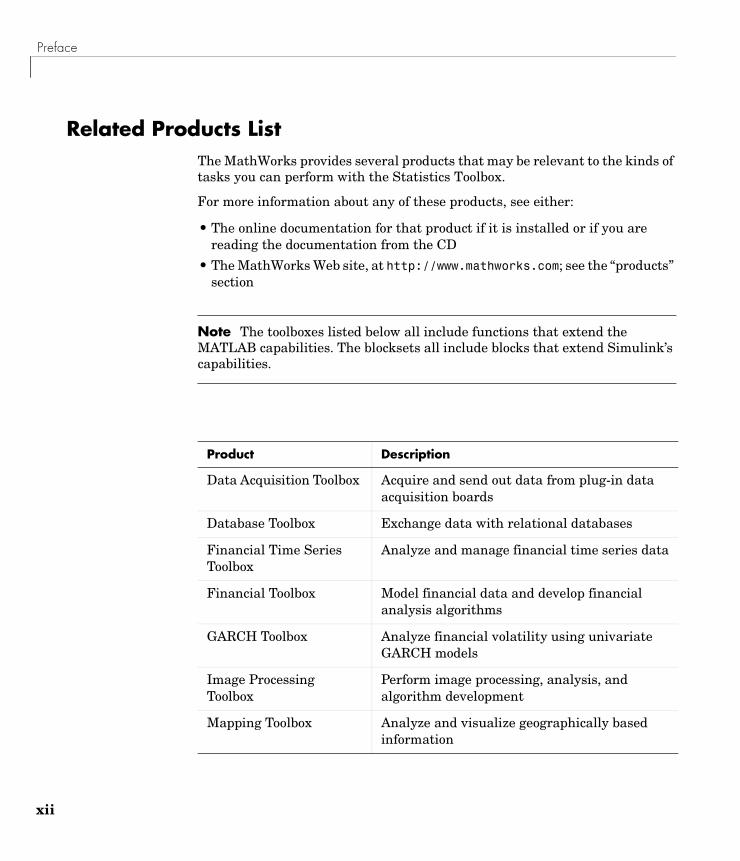
Related Products ListThe MathWorks provides several products that may be relevant to the kinds of tasks you can perform with the Statistics Toolbox.
For more information about any of these products, see either:
• The online documentation for that product if it is installed or if you are reading the documentation from the CD
• The MathWorks Web site, at http://www.mathworks.com; see the “products” section
Note The toolboxes listed below all include functions that extend the MATLAB capabilities. The blocksets all include blocks that extend Simulink’s capabilities.
Product Description
Data Acquisition Toolbox Acquire and send out data from plug-in data acquisition boards
Database Toolbox Exchange data with relational databases
Financial Time Series Toolbox
Analyze and manage financial time series data
Financial Toolbox Model financial data and develop financial analysis algorithms
GARCH Toolbox Analyze financial volatility using univariate GARCH models
Image Processing Toolbox
Perform image processing, analysis, and algorithm development
Mapping Toolbox Analyze and visualize geographically based information

Related Products List
Neural Network Toolbox Design and simulate neural networks
Optimization Toolbox Solve standard and large-scale optimization problems
Signal Processing Toolbox
Perform signal processing, analysis, and algorithm development
System Identification Toolbox
Create linear dynamic models from measured input-output data
Product Description
xiii

Preface
xiv
Typographical ConventionsThis manual uses some or all of these conventions.
Item Convention Example
Example code Monospace font To assign the value 5 to A, enter
A = 5
Function names, syntax, filenames, directory/folder names, and user input
Monospace font The cos function finds the cosine of each array element.Syntax line example isMLGetVar ML_var_name
Buttons and keys Boldface with book title caps Press the Enter key.
Literal strings (in syntax descriptions in reference chapters)
Monospace bold for literals f = freqspace(n,'whole')
Mathematicalexpressions
Italics for variablesStandard text font for functions, operators, and constants
This vector represents the polynomial p = x2 + 2x + 3.
MATLAB output Monospace font MATLAB responds withA =
5
Menu and dialog box titles Boldface with book title caps Choose the File Options menu.
New terms and for emphasis
Italics An array is an ordered collection of information.
Omitted input arguments (...) ellipsis denotes all of the input/output arguments from preceding syntaxes.
[c,ia,ib] = union(...)
String variables (from a finite list)
Monospace italics sysc = d2c(sysd,'method')

What Is the Statistics Toolbox? . . . . . . . . . . . 1-2
Primary Topic Areas . . . . . . . . . . . . . . . . 1-3
Random Numbers in Examples . . . . . . . . . . . 1-5
Mathematical Notation . . . . . . . . . . . . . . . 1-6
1
Introduction

1 Introduction
1-2
What Is the Statistics Toolbox?The Statistics Toolbox, for use with MATLAB, supplies basic statistics capability on the level of a first course in engineering or scientific statistics. The statistics functions it provides are building blocks suitable for use inside other analytical tools.
The Statistics Toolbox is a collection of tools built on the MATLAB“ numeric computing environment. The toolbox supports a wide range of common statistical tasks, from random number generation, to curve fitting, to design of experiments and statistical process control. The toolbox provides two categories of tools:
• Building-block probability and statistics functions
• Graphical, interactive tools
The first category of tools is made up of functions that you can call from the command line or from your own applications. Many of these functions are MATLAB M-files, series of MATLAB statements that implement specialized statistics algorithms. You can view the MATLAB code for these functions using the statement
type function_name
You can change the way any toolbox function works by copying and renaming the M-file, then modifying your copy. You can also extend the toolbox by adding your own M-files.
Secondly, the toolbox provides a number of interactive tools that let you access many of the functions through a graphical user interface (GUI). Together, the GUI-based tools provide an environment for polynomial fitting and prediction, as well as probability function exploration.

Primary Topic Areas
Primary Topic AreasThe Statistics Toolbox has more than 200 M-files, supporting work in these topical areas:
Probability DistributionsThe Statistics Toolbox supports 20 probability distributions. For each distribution there are five associated functions. They are
• Probability density function (pdf)
• Cumulative distribution function (cdf)
• Inverse of the cumulative distribution function
• Random number generator
• Mean and variance as a function of the parameters
For data-driven distributions (beta, binomial, exponential, gamma, normal, Poisson, uniform, and Weibull), the Statistics Toolbox has functions for computing parameter estimates and confidence intervals.
Descriptive StatisticsThe Statistics Toolbox provides functions for describing the features of a data sample. These descriptive statistics include measures of location and spread, percentile estimates and functions for dealing with data having missing values.
Linear ModelsIn the area of linear models, the Statistics Toolbox supports one-way, two-way, and higher-way analysis of variance (ANOVA), analysis of covariance (ANOCOVA), multiple linear regression, stepwise regression, response surface prediction, ridge regression, and one-way multivariate analysis of variance (MANOVA). It supports nonparametric versions of one- and two-way ANOVA. It also supports multiple comparisons of the estimates produced by ANOVA and ANOCOVA functions.
Nonlinear ModelsFor nonlinear models, the Statistics Toolbox provides functions for parameter estimation, interactive prediction and visualization of multidimensional nonlinear fits, and confidence intervals for parameters and predicted values. It
1-3
1 Introduction
1-4
provides functions for using classification and regression trees to approximate regression relationships.
Hypothesis TestsThe Statistics Toolbox also provides functions that do the most common tests of hypothesis — t-tests, Z-tests, nonparametric tests, and distribution tests.
Multivariate StatisticsThe Statistics Toolbox supports methods in multivariate statistics, including principal components analysis, factor analysis, one-way multivariate analysis of variance, cluster analysis, and classical multidimensional scaling.
Statistical PlotsThe Statistics Toolbox adds box plots, normal probability plots, Weibull probability plots, control charts, and quantile-quantile plots to the arsenal of graphs in MATLAB. There is also extended support for polynomial curve fitting and prediction. There are functions to create scatter plots or matrices of scatter plots for grouped data, and to identify points interactively on such plots. There is a function to interactively explore a fitted regression model.
Statistical Process Control (SPC)For SPC, the Statistics Toolbox provides functions for plotting common control charts and performing process capability studies.
Design of Experiments (DOE)The Statistics Toolbox supports full and fractional factorial designs, response surface designs, and D-optimal designs. There are functions for generating designs, augmenting designs, and optimally assigning units with fixed covariates.

Random Numbers in Examples
Random Numbers in ExamplesThe random number generation functions for various probability distributions are based on the primitive functions, randn and rand. There are many examples that start by generating data using random numbers. To duplicate the results in these examples, first execute the commands below.
seed = 931316785;rand('seed',seed);randn('seed',seed);
You might want to save these commands in an M-file script called initseed.m. Then, instead of three separate commands, you need only type initseed.
Note For rand and randn, the 'seed' syntax is replaced by the 'state' syntax in MATLAB Version 5. Although use of the 'seed' syntax is backward compatible in MATLAB Version 6.5, you should avoid its use. This book will be updated to use the 'state' syntax in a future release.
1-5

1 Introduction
1-6
Mathematical NotationThis manual and the Statistics Toolbox functions use the following mathematical notation conventions.
β Parameters in a linear model.
E(x) Expected value of x.
f(x|a,b) Probability density function. x is the independent variable; a and b are fixed parameters.
F(x|a,b) Cumulative distribution function.
I([a, b]) or I[a, b]
Indicator function. In this example the function takes the value 1 on the closed interval from a to b and is 0 elsewhere.
p and q p is the probability of some event. q is the probability of ~p, so q = 1-p.
E x( ) tf t( ) td∫=

Introduction . . . . . . . . . . . . . . . . . . . . 2-2
Overview of the Functions . . . . . . . . . . . . . 2-4Probability Density Function (pdf) . . . . . . . . . . . 2-4Cumulative Distribution Function (cdf) . . . . . . . . . 2-5Inverse Cumulative Distribution Function . . . . . . . . 2-5Random Number Generator . . . . . . . . . . . . . . 2-7Mean and Variance as a Function of Parameters . . . . . . 2-9
Overview of the Distributions . . . . . . . . . . . . 2-11Beta Distribution . . . . . . . . . . . . . . . . . . 2-11Binomial Distribution . . . . . . . . . . . . . . . . . 2-13Chi-Square Distribution . . . . . . . . . . . . . . . . 2-16Noncentral Chi-Square Distribution . . . . . . . . . . . 2-17Discrete Uniform Distribution . . . . . . . . . . . . . 2-19Exponential Distribution . . . . . . . . . . . . . . . 2-20F Distribution . . . . . . . . . . . . . . . . . . . . 2-22Noncentral F Distribution . . . . . . . . . . . . . . . 2-23Gamma Distribution . . . . . . . . . . . . . . . . . 2-25Geometric Distribution . . . . . . . . . . . . . . . . 2-27Hypergeometric Distribution . . . . . . . . . . . . . . 2-28Lognormal Distribution . . . . . . . . . . . . . . . . 2-29Negative Binomial Distribution . . . . . . . . . . . . . 2-31Normal Distribution . . . . . . . . . . . . . . . . . 2-34Poisson Distribution . . . . . . . . . . . . . . . . . 2-36Rayleigh Distribution . . . . . . . . . . . . . . . . . 2-38Student’s t Distribution . . . . . . . . . . . . . . . . 2-39Noncentral t Distribution . . . . . . . . . . . . . . . 2-40Weibull Distribution . . . . . . . . . . . . . . . . . 2-43
2
Probability Distributions

2 Probability Distributions
2-2
IntroductionProbability distributions arise from experiments where the outcome is subject to chance. The nature of the experiment dictates which probability distributions may be appropriate for modeling the resulting random outcomes. There are two types of probability distributions – continuous and discrete.
Suppose you are studying a machine that produces videotape. One measure of the quality of the tape is the number of visual defects per hundred feet of tape. The result of this experiment is an integer, since you cannot observe 1.5 defects. To model this experiment you should use a discrete probability distribution.
A measure affecting the cost and quality of videotape is its thickness. Thick tape is more expensive to produce, while variation in the thickness of the tape on the reel increases the likelihood of breakage. Suppose you measure the thickness of the tape every 1000 feet. The resulting numbers can take a continuum of possible values, which suggests using a continuous probability distribution to model the results.
Using a probability model does not allow you to predict the result of any individual experiment but you can determine the probability that a given outcome will fall inside a specific range of values.
Continuous (data) Continuous (statistics) Discrete
Beta Chi-square Binomial
Exponential Noncentral Chi-square Discrete Uniform
Gamma F Geometric
Lognormal Noncentral F Hypergeometric
Normal t Negative Binomial
Rayleigh Noncentral t Poisson
Uniform
Weibull

Introduction
This following two sections provide more information about the available distributions:
• “Overview of the Functions” on page 2-4
• “Overview of the Distributions” on page 2-11
2-3

2 Probability Distributions
2-4
Overview of the FunctionsThe Statistics Toolbox provides five functions for each distribution. They are discussed in the following sections:
• “Probability Density Function (pdf)” on page 2-4
• “Cumulative Distribution Function (cdf)” on page 2-5
• “Inverse Cumulative Distribution Function” on page 2-5
• “Random Number Generator” on page 2-7
• “Mean and Variance as a Function of Parameters” on page 2-9
Probability Density Function (pdf)The probability density function (pdf) has a different meaning depending on whether the distribution is discrete or continuous.
For discrete distributions, the pdf is the probability of observing a particular outcome. In our videotape example, the probability that there is exactly one defect in a given hundred feet of tape is the value of the pdf at 1.
Unlike discrete distributions, the pdf of a continuous distribution at a value is not the probability of observing that value. For continuous distributions the probability of observing any particular value is zero. To get probabilities you must integrate the pdf over an interval of interest. For example the probability of the thickness of a videotape being between one and two millimeters is the integral of the appropriate pdf from one to two.
A pdf has two theoretical properties:
• The pdf is zero or positive for every possible outcome.
• The integral of a pdf over its entire range of values is one.
A pdf is not a single function. Rather a pdf is a family of functions characterized by one or more parameters. Once you choose (or estimate) the parameters of a pdf, you have uniquely specified the function.
The pdf function call has the same general format for every distribution in the Statistics Toolbox. The following commands illustrate how to call the pdf for the normal distribution.
x = [-3:0.1:3];f = normpdf(x,0,1);

Overview of the Functions
The variable f contains the density of the normal pdf with parameters µ=0 and σ=1 at the values in x. The first input argument of every pdf is the set of values for which you want to evaluate the density. Other arguments contain as many parameters as are necessary to define the distribution uniquely. The normal distribution requires two parameters; a location parameter (the mean, µ) and a scale parameter (the standard deviation, σ).
Cumulative Distribution Function (cdf)If f is a probability density function for random variable X, the associated cumulative distribution function (cdf) F is
The cdf of a value x, F(x), is the probability of observing any outcome less than or equal to x.
A cdf has two theoretical properties:
• The cdf ranges from 0 to 1.
• If y > x, then the cdf of y is greater than or equal to the cdf of x.
The cdf function call has the same general format for every distribution in the Statistics Toolbox. The following commands illustrate how to call the cdf for the normal distribution.
x = [-3:0.1:3];p = normcdf(x,0,1);
The variable p contains the probabilities associated with the normal cdf with parameters µ=0 and σ=1 at the values in x. The first input argument of every cdf is the set of values for which you want to evaluate the probability. Other arguments contain as many parameters as are necessary to define the distribution uniquely.
Inverse Cumulative Distribution FunctionThe inverse cumulative distribution function returns critical values for hypothesis testing given significance probabilities. To understand the relationship between a continuous cdf and its inverse function, try the following:
F x( ) P X x≤( ) f t( ) td∞–
x
∫= =
2-5

2 Probability Distributions
2-6
x = [-3:0.1:3];xnew = norminv(normcdf(x,0,1),0,1);
How does xnew compare with x? Conversely, try this:
p = [0.1:0.1:0.9];pnew = normcdf(norminv(p,0,1),0,1);
How does pnew compare with p?
Calculating the cdf of values in the domain of a continuous distribution returns probabilities between zero and one. Applying the inverse cdf to these probabilities yields the original values.
For discrete distributions, the relationship between a cdf and its inverse function is more complicated. It is likely that there is no x value such that the cdf of x yields p. In these cases the inverse function returns the first value x such that the cdf of x equals or exceeds p. Try this:
x = [0:10];y = binoinv(binocdf(x,10,0.5),10,0.5);
How does x compare with y?
The commands below illustrate the problem with reconstructing the probability p from the value x for discrete distributions.
p = [0.1:0.2:0.9];pnew = binocdf(binoinv(p,10,0.5),10,0.5)
pnew =
0.1719 0.3770 0.6230 0.8281 0.9453
The inverse function is useful in hypothesis testing and production of confidence intervals. Here is the way to get a 99% confidence interval for a normally distributed sample.
p = [0.005 0.995];x = norminv(p,0,1)
x =
-2.5758 2.5758

Overview of the Functions
The variable x contains the values associated with the normal inverse function with parameters µ=0 and σ=1 at the probabilities in p. The difference p(2)-p(1) is 0.99. Thus, the values in x define an interval that contains 99% of the standard normal probability.
The inverse function call has the same general format for every distribution in the Statistics Toolbox. The first input argument of every inverse function is the set of probabilities for which you want to evaluate the critical values. Other arguments contain as many parameters as are necessary to define the distribution uniquely.
Random Number GeneratorThe methods for generating random numbers from any distribution all start with uniform random numbers. Once you have a uniform random number generator, you can produce random numbers from other distributions either directly or by using inversion or rejection methods, described below. See “Syntax for Random Number Functions” on page 2-8 for details on using generator functions.
DirectDirect methods flow from the definition of the distribution.
As an example, consider generating binomial random numbers. You can think of binomial random numbers as the number of heads in n tosses of a coin with probability p of a heads on any toss. If you generate n uniform random numbers and count the number that are greater than p, the result is binomial with parameters n and p.
InversionThe inversion method works due to a fundamental theorem that relates the uniform distribution to other continuous distributions.
If F is a continuous distribution with inverse F -1, and U is a uniform random number, then F -1(U) has distribution F.
So, you can generate a random number from a distribution by applying the inverse function for that distribution to a uniform random number. Unfortunately, this approach is usually not the most efficient.
2-7

2 Probability Distributions
2-8
RejectionThe functional form of some distributions makes it difficult or time consuming to generate random numbers using direct or inversion methods. Rejection methods can sometimes provide an elegant solution in these cases.
Suppose you want to generate random numbers from a distribution with pdf f. To use rejection methods you must first find another density, g, and a constant, c, so that the inequality below holds.
You then generate the random numbers you want using the following steps:
1 Generate a random number x from distribution G with density g.
2 Form the ratio .
3 Generate a uniform random number u.
4 If the product of u and r is less than one, return x.
5 Otherwise repeat steps one to three.
For efficiency you need a cheap method for generating random numbers from G, and the scalar c should be small. The expected number of iterations is c.
Syntax for Random Number FunctionsYou can generate random numbers from each distribution. This function provides a single random number or a matrix of random numbers, depending on the arguments you specify in the function call.
For example, here is the way to generate random numbers from the beta distribution. Four statements obtain random numbers: the first returns a single number, the second returns a 2-by-2 matrix of random numbers, and the third and fourth return 2-by-3 matrices of random numbers.
a = 1;b = 2;c = [.1 .5; 1 2];d = [.25 .75; 5 10];m = [2 3];
f x( ) cg x( ) x∀≤
r cg x( )f x( )--------------=

Overview of the Functions
nrow = 2;ncol = 3;
r1 = betarnd(a,b)r1 =
0.4469
r2 = betarnd(c,d)r2 =
0.8931 0.4832 0.1316 0.2403
r3 = betarnd(a,b,m)r3 =
0.4196 0.6078 0.1392 0.0410 0.0723 0.0782
r4 = betarnd(a,b,nrow,ncol)r4 =
0.0520 0.3975 0.1284 0.3891 0.1848 0.5186
Mean and Variance as a Function of ParametersThe mean and variance of a probability distribution are generally simple functions of the parameters of the distribution. The Statistics Toolbox functions ending in "stat" all produce the mean and variance of the desired distribution for the given parameters.
The example below shows a contour plot of the mean of the Weibull distribution as a function of the parameters.
x = (0.5:0.1:5);y = (1:0.04:2);[X,Y] = meshgrid(x,y);Z = weibstat(X,Y);[c,h] = contour(x,y,Z,[0.4 0.6 1.0 1.8]);clabel(c);
2-9

2 Probability Distributions
2-1
1 2 3 4 51
1.2
1.4
1.6
1.8
2
0.4
0.6
1
1.8
0

Overview of the Distributions
Overview of the DistributionsThe following sections describe the available probability distributions:
• “Beta Distribution” on page 2-11
• “Binomial Distribution” on page 2-13
• “Chi-Square Distribution” on page 2-16
• “Noncentral Chi-Square Distribution” on page 2-17
• “Discrete Uniform Distribution” on page 2-19
• “Exponential Distribution” on page 2-20
• “F Distribution” on page 2-22
• “Noncentral F Distribution” on page 2-23
• “Gamma Distribution” on page 2-25
• “Geometric Distribution” on page 2-27
• “Hypergeometric Distribution” on page 2-28
• “Lognormal Distribution” on page 2-29
• “Negative Binomial Distribution” on page 2-31
• “Normal Distribution” on page 2-34
• “Poisson Distribution” on page 2-36
• “Rayleigh Distribution” on page 2-38
• “Student’s t Distribution” on page 2-39
• “Noncentral t Distribution” on page 2-40
• “Uniform (Continuous) Distribution” on page 2-42
• “Weibull Distribution” on page 2-43
Beta DistributionThe following sections provide an overview of the beta distribution.
Background on the Beta DistributionThe beta distribution describes a family of curves that are unique in that they are nonzero only on the interval (0 1). A more general version of the function assigns parameters to the end-points of the interval.
The beta cdf is the same as the incomplete beta function.
2-11

2 Probability Distributions
2-1
The beta distribution has a functional relationship with the t distribution. If Y is an observation from Student’s t distribution with ν degrees of freedom, then the following transformation generates X, which is beta distributed.
if then
The Statistics Toolbox uses this relationship to compute values of the t cdf and inverse function as well as generating t distributed random numbers.
Definition of the Beta DistributionThe beta pdf is
where B( · ) is the Beta function. The indicator function I(0,1)(x) ensures that only values of x in the range (0 1) have nonzero probability.
Parameter Estimation for the Beta DistributionSuppose you are collecting data that has hard lower and upper bounds of zero and one respectively. Parameter estimation is the process of determining the parameters of the beta distribution that fit this data best in some sense.
One popular criterion of goodness is to maximize the likelihood function. The likelihood has the same form as the beta pdf. But for the pdf, the parameters are known constants and the variable is x. The likelihood function reverses the roles of the variables. Here, the sample values (the x’s) are already observed. So they are the fixed constants. The variables are the unknown parameters. Maximum likelihood estimation (MLE) involves calculating the values of the parameters that give the highest likelihood given the particular set of data.
The function betafit returns the MLEs and confidence intervals for the parameters of the beta distribution. Here is an example using random numbers from the beta distribution with a = 5 and b = 0.2.
r = betarnd(5,0.2,100,1);[phat, pci] = betafit(r)
X 12--- 1
2--- Y
ν Y2+
--------------------+=
Y t ν( ) ∼ X β ν2--- ν
2---,
∼
y f x a b,( ) 1B a b,( )-------------------xa 1– 1 x–( )b 1– I 0 1,( ) x( )= =
2

Overview of the Distributions
phat = 4.5330 0.2301
pci = 2.8051 0.1771 6.2610 0.2832
The MLE for parameter a is 4.5330, compared to the true value of 5. The 95% confidence interval for a goes from 2.8051 to 6.2610, which includes the true value.
Similarly the MLE for parameter b is 0.2301, compared to the true value of 0.2. The 95% confidence interval for b goes from 0.1771 to 0.2832, which also includes the true value. Of course, in this made-up example we know the “true value.” In experimentation we do not.
Example and Plot of the Beta DistributionThe shape of the beta distribution is quite variable depending on the values of the parameters, as illustrated by the plot below.
The constant pdf (the flat line) shows that the standard uniform distribution is a special case of the beta distribution.
Binomial DistributionThe following sections provide an overview of the binomial distribution.
0 0.2 0.4 0.6 0.8 10
0.5
1
1.5
2
2.5
a = b = 1
a = b = 4 a = b = 0.75
2-13

2 Probability Distributions
2-1
Background of the Binomial DistributionThe binomial distribution models the total number of successes in repeated trials from an infinite population under the following conditions:
• Only two outcomes are possible on each of n trials.
• The probability of success for each trial is constant.
• All trials are independent of each other.
James Bernoulli derived the binomial distribution in 1713 (Ars Conjectandi). Earlier, Blaise Pascal had considered the special case where p = 1/2.
Definition of the Binomial DistributionThe binomial pdf is
where and .
The binomial distribution is discrete. For zero and for positive integers less than n, the pdf is nonzero.
Parameter Estimation for the Binomial DistributionSuppose you are collecting data from a widget manufacturing process, and you record the number of widgets within specification in each batch of 100. You might be interested in the probability that an individual widget is within specification. Parameter estimation is the process of determining the parameter, p, of the binomial distribution that fits this data best in some sense.
One popular criterion of goodness is to maximize the likelihood function. The likelihood has the same form as the binomial pdf above. But for the pdf, the parameters (n and p) are known constants and the variable is x. The likelihood function reverses the roles of the variables. Here, the sample values (the x’s) are already observed. So they are the fixed constants. The variables are the unknown parameters. MLE involves calculating the value of p that give the highest likelihood given the particular set of data.
y f x n p,( )nx pxq 1 x–( )I 0 1 … n, , ,( ) x( )= =
nx n!
x! n x–( )!------------------------ = q 1 p–=
4

Overview of the Distributions
The function binofit returns the MLEs and confidence intervals for the parameters of the binomial distribution. Here is an example using random numbers from the binomial distribution with n = 100 and p = 0.9.
r = binornd(100,0.9)
r = 88
[phat, pci] = binofit(r,100)
phat = 0.8800
pci = 0.7998 0.9364
The MLE for parameter p is 0.8800, compared to the true value of 0.9. The 95% confidence interval for p goes from 0.7998 to 0.9364, which includes the true value. Of course, in this made-up example we know the “true value” of p. In experimentation we do not.
Example and Plot of the Binomial DistributionThe following commands generate a plot of the binomial pdf for n = 10 and p = 1/2.
x = 0:10;y = binopdf(x,10,0.5);plot(x,y,'+')
2-15

2 Probability Distributions
2-1
Chi-Square DistributionThe following sections provide an overview of the χ2 distribution.
Background of the Chi-Square DistributionThe χ2 distribution is a special case of the gamma distribution where b = 2 in the equation for gamma distribution below.
The χ2 distribution gets special attention because of its importance in normal sampling theory. If a set of n observations is normally distributed with variance σ2, and s2 is the sample standard deviation, then
The Statistics Toolbox uses the above relationship to calculate confidence intervals for the estimate of the normal parameter σ2 in the function normfit.
0 2 4 6 8 100
0.05
0.1
0.15
0.2
0.25
y f x a b,( ) 1
baΓ a( )------------------xa 1– e
xb---–
= =
n 1–( )s2
σ2----------------------- χ2 n 1–( )∼
6

Overview of the Distributions
Definition of the Chi-Square DistributionThe χ2 pdf is
where Γ( · ) is the Gamma function, and ν is the degrees of freedom.
Example and Plot of the Chi-Square DistributionThe χ2 distribution is skewed to the right especially for few degrees of freedom (ν). The plot shows the χ2 distribution with four degrees of freedom.
x = 0:0.2:15;y = chi2pdf(x,4);plot(x,y)
Noncentral Chi-Square DistributionThe following sections provide an overview of the noncentral χ2 distribution.
Background of the Noncentral Chi-Square DistributionThe χ2 distribution is actually a simple special case of the noncentral chi-square distribution. One way to generate random numbers with a χ2 distribution (with ν degrees of freedom) is to sum the squares of ν standard normal random numbers (mean equal to zero.)
What if we allow the normally distributed quantities to have a mean other than zero? The sum of squares of these numbers yields the noncentral chi-square
y f x ν( ) x ν 2–( ) 2⁄ e x– 2⁄
2
v2---Γ ν 2⁄( )
-------------------------------------= =
0 5 10 150
0.05
0.1
0.15
0.2
2-17
2 Probability Distributions
2-1
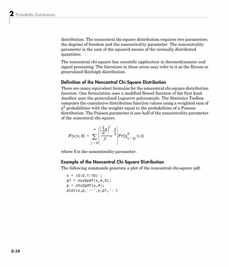
distribution. The noncentral chi-square distribution requires two parameters; the degrees of freedom and the noncentrality parameter. The noncentrality parameter is the sum of the squared means of the normally distributed quantities.
The noncentral chi-square has scientific application in thermodynamics and signal processing. The literature in these areas may refer to it as the Ricean or generalized Rayleigh distribution.
Definition of the Noncentral Chi-Square DistributionThere are many equivalent formulas for the noncentral chi-square distribution function. One formulation uses a modified Bessel function of the first kind. Another uses the generalized Laguerre polynomials. The Statistics Toolbox computes the cumulative distribution function values using a weighted sum of χ2 probabilities with the weights equal to the probabilities of a Poisson distribution. The Poisson parameter is one-half of the noncentrality parameter of the noncentral chi-square.
where δ is the noncentrality parameter.
Example of the Noncentral Chi-Square DistributionThe following commands generate a plot of the noncentral chi-square pdf.
x = (0:0.1:10)';p1 = ncx2pdf(x,4,2);p = chi2pdf(x,4);plot(x,p,'--',x,p1,'-')
F x ν δ,( )
12---δ j
j!--------------e
δ2---–
Pr χν 2j+
2 x≤[ ]
j 0=
∞
∑=
8

Overview of the Distributions
Discrete Uniform DistributionThe following sections provide an overview of the discrete uniform distribution.
Background of the Discrete Uniform DistributionThe discrete uniform distribution is a simple distribution that puts equal weight on the integers from one to N.
Definition of the Discrete Uniform DistributionThe discrete uniform pdf is
Example and Plot of the Discrete Uniform DistributionAs for all discrete distributions, the cdf is a step function. The plot shows the discrete uniform cdf for N = 10.
x = 0:10;y = unidcdf(x,10);stairs(x,y)set(gca,'Xlim',[0 11])
0 2 4 6 8 100
0.05
0.1
0.15
0.2
y f x N( ) 1N---- I 1 … N, ,( ) x( )= =
2-19

2 Probability Distributions
2-2
To pick a random sample of 10 from a list of 553 items:
numbers = unidrnd(553,1,10)
numbers =
293 372 5 213 37 231 380 326 515 468
Exponential DistributionThe following sections provide an overview of the exponential distribution.
Background of the Exponential DistributionLike the chi-square distribution, the exponential distribution is a special case of the gamma distribution (obtained by setting a = 1)
where Γ( · ) is the Gamma function.
The exponential distribution is special because of its utility in modeling events that occur randomly over time. The main application area is in studies of lifetimes.
Definition of the Exponential DistributionThe exponential pdf is
0 2 4 6 8 100
0.2
0.4
0.6
0.8
1
y f x a b,( ) 1
baΓ a( )------------------xa 1– e
xb---–
= =
y f x µ( ) 1µ---e
xµ---–
= =
0

Overview of the Distributions
Parameter Estimation for the Exponential DistributionSuppose you are stress testing light bulbs and collecting data on their lifetimes. You assume that these lifetimes follow an exponential distribution. You want to know how long you can expect the average light bulb to last. Parameter estimation is the process of determining the parameters of the exponential distribution that fit this data best in some sense.
One popular criterion of goodness is to maximize the likelihood function. The likelihood has the same form as the exponential pdf above. But for the pdf, the parameters are known constants and the variable is x. The likelihood function reverses the roles of the variables. Here, the sample values (the x’s) are already observed. So they are the fixed constants. The variables are the unknown parameters. MLE involves calculating the values of the parameters that give the highest likelihood given the particular set of data.
The function expfit returns the MLEs and confidence intervals for the parameters of the exponential distribution. Here is an example using random numbers from the exponential distribution with µ = 700.
lifetimes = exprnd(700,100,1);[muhat, muci] = expfit(lifetimes)
muhat =
672.8207
muci =
547.4338 810.9437
The MLE for parameter µ is 672, compared to the true value of 700. The 95% confidence interval for µ goes from 547 to 811, which includes the true value.
In our life tests we do not know the true value of µ so it is nice to have a confidence interval on the parameter to give a range of likely values.
Example and Plot of the Exponential DistributionFor exponentially distributed lifetimes, the probability that an item will survive an extra unit of time is independent of the current age of the item. The example shows a specific case of this special property.
2-21

2 Probability Distributions
2-2
l = 10:10:60;lpd = l+0.1;deltap = (expcdf(lpd,50)-expcdf(l,50))./(1-expcdf(l,50))
deltap = 0.0020 0.0020 0.0020 0.0020 0.0020 0.0020
The plot below shows the exponential pdf with its parameter (and mean), µ, set to 2.
x = 0:0.1:10;y = exppdf(x,2);plot(x,y)
F DistributionThe following sections provide an overview of the F distribution.
Background of the F distributionThe F distribution has a natural relationship with the chi-square distribution. If χ1 and χ2 are both chi-square with ν1 and ν2 degrees of freedom respectively, then the statistic F below is F distributed.
0 2 4 6 8 100
0.1
0.2
0.3
0.4
0.5
F ν1 ν2,( )
χ1ν1------
χ2ν2------------=
2

Overview of the Distributions
The two parameters, ν1 and ν2, are the numerator and denominator degrees of freedom. That is, ν1 and ν2 are the number of independent pieces information used to calculate χ1 and χ2 respectively.
Definition of the F distributionThe pdf for the F distribution is
where Γ( · ) is the Gamma function.
Example and Plot of the F distributionThe most common application of the F distribution is in standard tests of hypotheses in analysis of variance and regression.
The plot shows that the F distribution exists on the positive real numbers and is skewed to the right.
x = 0:0.01:10;y = fpdf(x,5,3);plot(x,y)
Noncentral F DistributionThe following sections provide an overview of the noncentral F distribution.
y f x ν1 ν2,( )Γ
ν1 ν2+( )2
-----------------------
Γν12------ Γ
ν22------
--------------------------------ν1ν2------
ν1
2----- x
ν1 2–2
--------------
1ν1ν2------ x+
ν1 ν2+2
-------------------------------------------------------------= =
0 2 4 6 8 100
0.2
0.4
0.6
0.8
2-23

2 Probability Distributions
2-2
Background of the Noncentral F DistributionAs with the χ2 distribution, the F distribution is a special case of the noncentral F distribution. The F distribution is the result of taking the ratio of two χ2 random variables each divided by its degrees of freedom.
If the numerator of the ratio is a noncentral chi-square random variable divided by its degrees of freedom, the resulting distribution is the noncentral F distribution.
The main application of the noncentral F distribution is to calculate the power of a hypothesis test relative to a particular alternative.
Definition of the Noncentral F DistributionSimilar to the noncentral χ2 distribution, the toolbox calculates noncentral F distribution probabilities as a weighted sum of incomplete beta functions using Poisson probabilities as the weights.
I(x|a,b) is the incomplete beta function with parameters a and b, and δ is the noncentrality parameter.
Example and Plot of the Noncentral F DistributionThe following commands generate a plot of the noncentral F pdf.
x = (0.01:0.1:10.01)';p1 = ncfpdf(x,5,20,10);p = fpdf(x,5,20);plot(x,p,'--',x,p1,'-')
F x ν1 ν2 δ, ,( )
12---δ j
j!--------------e
δ2---–
Iν1 x⋅
ν2 ν+ 1 x⋅-------------------------
ν12------ j+
ν22------,
j 0=
∞
∑=
4
Overview of the Distributions
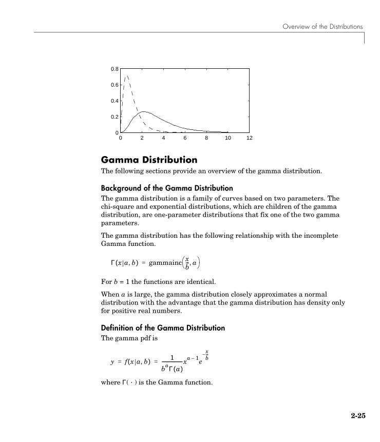
Gamma DistributionThe following sections provide an overview of the gamma distribution.
Background of the Gamma DistributionThe gamma distribution is a family of curves based on two parameters. The chi-square and exponential distributions, which are children of the gamma distribution, are one-parameter distributions that fix one of the two gamma parameters.
The gamma distribution has the following relationship with the incomplete Gamma function.
For b = 1 the functions are identical.
When a is large, the gamma distribution closely approximates a normal distribution with the advantage that the gamma distribution has density only for positive real numbers.
Definition of the Gamma DistributionThe gamma pdf is
where Γ( · ) is the Gamma function.
0 2 4 6 8 10 120
0.2
0.4
0.6
0.8
Γ x a b,( ) gammainc xb--- a, =
y f x a b,( ) 1
baΓ a( )------------------xa 1– e
xb---–
= =
2-25

2 Probability Distributions
2-2
Parameter Estimation for the Gamma DistributionSuppose you are stress testing computer memory chips and collecting data on their lifetimes. You assume that these lifetimes follow a gamma distribution. You want to know how long you can expect the average computer memory chip to last. Parameter estimation is the process of determining the parameters of the gamma distribution that fit this data best in some sense.
One popular criterion of goodness is to maximize the likelihood function. The likelihood has the same form as the gamma pdf above. But for the pdf, the parameters are known constants and the variable is x. The likelihood function reverses the roles of the variables. Here, the sample values (the x’s) are already observed. So they are the fixed constants. The variables are the unknown parameters. MLE involves calculating the values of the parameters that give the highest likelihood given the particular set of data.
The function gamfit returns the MLEs and confidence intervals for the parameters of the gamma distribution. Here is an example using random numbers from the gamma distribution with a = 10 and b = 5.
lifetimes = gamrnd(10,5,100,1);[phat, pci] = gamfit(lifetimes)
phat =
10.9821 4.7258
pci =
7.4001 3.1543 14.5640 6.2974
Note phat(1) = and phat(2) = . The MLE for parameter a is 10.98, compared to the true value of 10. The 95% confidence interval for a goes from 7.4 to 14.6, which includes the true value.
Similarly the MLE for parameter b is 4.7, compared to the true value of 5. The 95% confidence interval for b goes from 3.2 to 6.3, which also includes the true value.
In our life tests we do not know the true value of a and b so it is nice to have a confidence interval on the parameters to give a range of likely values.
a� b�
6
Overview of the Distributions
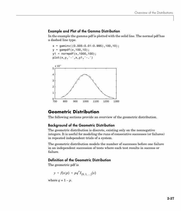
Example and Plot of the Gamma DistributionIn the example the gamma pdf is plotted with the solid line. The normal pdf has a dashed line type.
x = gaminv((0.005:0.01:0.995),100,10);y = gampdf(x,100,10);y1 = normpdf(x,1000,100);plot(x,y,'-',x,y1,'-.')
Geometric DistributionThe following sections provide an overview of the geometric distribution.
Background of the Geometric DistributionThe geometric distribution is discrete, existing only on the nonnegative integers. It is useful for modeling the runs of consecutive successes (or failures) in repeated independent trials of a system.
The geometric distribution models the number of successes before one failure in an independent succession of tests where each test results in success or failure.
Definition of the Geometric DistributionThe geometric pdf is
where q = 1 – p.
700 800 900 1000 1100 1200 13000
1
2
3
4
5x 10⁻³
y f x p( ) pqxI 0 1 …, ,( ) x( )= =
2-27

2 Probability Distributions
2-2
Example and Plot of the Geometric DistributionSuppose the probability of a five-year-old battery failing in cold weather is 0.03. What is the probability of starting 25 consecutive days during a long cold snap?
1 - geocdf(25,0.03)
ans =
0.4530
The plot shows the cdf for this scenario.
x = 0:25;y = geocdf(x,0.03);stairs(x,y)
Hypergeometric DistributionThe following sections provide an overview of the hypergeometric distribution.
Background of the Hypergeometric DistributionThe hypergeometric distribution models the total number of successes in a fixed size sample drawn without replacement from a finite population.
The distribution is discrete, existing only for nonnegative integers less than the number of samples or the number of possible successes, whichever is greater. The hypergeometric distribution differs from the binomial only in that the population is finite and the sampling from the population is without replacement.
0 5 10 15 20 250
0.2
0.4
0.6
8

Overview of the Distributions
The hypergeometric distribution has three parameters that have direct physical interpretations. M is the size of the population. K is the number of items with the desired characteristic in the population. n is the number of samples drawn. Sampling “without replacement” means that once a particular sample is chosen, it is removed from the relevant population for all subsequent selections.
Definition of the Hypergeometric DistributionThe hypergeometric pdf is
Example and Plot of the Hypergeometric DistributionThe plot shows the cdf of an experiment taking 20 samples from a group of 1000 where there are 50 items of the desired type.
x = 0:10;y = hygecdf(x,1000,50,20);stairs(x,y)
Lognormal DistributionThe following sections provide an overview of the lognormal distribution.
y f x M K n, ,( )
Kx M K–
n x–
Mn
-------------------------------= =
0 2 4 6 8 100.2
0.4
0.6
0.8
1
2-29

2 Probability Distributions
2-3
Background of the Lognormal DistributionThe normal and lognormal distributions are closely related. If X is distributed lognormal with parameters µ and σ2, then lnX is distributed normal with parameters µ and σ2.
The lognormal distribution is applicable when the quantity of interest must be positive, since lnX exists only when the random variable X is positive. Economists often model the distribution of income using a lognormal distribution.
Definition of the Lognormal DistributionThe lognormal pdf is
Example and Plot of the Lognormal DistributionSuppose the income of a family of four in the United States follows a lognormal distribution with µ = log(20,000) and σ2 = 1.0. Plot the income density.
x = (10:1000:125010)';y = lognpdf(x,log(20000),1.0);plot(x,y)set(gca,'xtick',[0 30000 60000 90000 120000])set(gca,'xticklabel',str2mat('0','$30,000','$60,000',...
'$90,000','$120,000'))
y f x µ σ,( ) 1xσ 2π------------------e
lnx µ–( )– 2
2σ2----------------------------
= =
0 $30,000 $60,000 $90,000 $120,0000
0.5
1
1.5
2
2.5
3
3.5x 10
−5
0

Overview of the Distributions
Negative Binomial DistributionThe following sections provide an overview of the negative binomial distribution.
• “Background of the Negative Binomial Distribution” on page 2-31
• “Definition of the Negative Binomial Distribution” on page 2-31
• “Parameter Estimation for the Negative Binomial Distribution” on page 2-32
• “Example and Plot of the Negative Binomial Distribution” on page 2-33
Background of the Negative Binomial DistributionIn its simplest form, the negative binomial distribution models the number of successes before a specified number of failures is reached in an independent series of repeated identical trials. It can also be thought of as modelling the total number of trials required before a specified number of successes, thus motivating its name as the "inverse" of the binomial distribution. Its parameters are the probability of success in a single trial, , and the number of failures, . A special case of the negative binomial distribution, when , is the geometric distribution (also known as the Pascal distribution), which models the number of successes before the first failure.
More generally, the parameter can take on non-integer values. This form of the negative binomial has no interpretation in terms of repeated trials, but, like the Poisson distribution, it is useful in modelling count data. It is, however, more general than the Poisson, because the negative binomial has a variance that is greater than its mean, often making it suitable for count data that do not meet the assumptions of the Poisson distribution. In the limit, as the parameter increases to infinity, the negative binomial distribution approaches the Poisson distribution.
Definition of the Negative Binomial DistributionWhen the parameter is an integer, the negative binomial pdf is
where . When is non-integer, the binomial coefficient in the definition of the pdf is replaced by the equivalent expression
pr r 1=
r
r
r
y f x r p,( ) r x 1–+x
prqxI 0 1 …, ,( ) x( )= =
q 1 p–= r
2-31

2 Probability Distributions
2-3
Parameter Estimation for the Negative Binomial DistributionSuppose you are collecting data on the number of auto accidents on a busy highway, and would like to be able to model the number of accidents per day. Because these are count data, and because there are a very large number of cars and a small probability of an accident for any specific car, you might think to use the Poisson distribution. However, the probability of having an accident is likely to vary from day to day as the weather and amount of traffic change, and so the assumptions needed for the Poisson distribution are not met. In particular, the variance of this type of count data sometimes exceeds the mean by a large amount. The data below exhibit this effect: most days have few or no accidents, and a few days have a large number.
accident = [2 3 4 2 3 1 12 8 14 31 23 1 10 7 0];mean(accident)ans = 8.0667
var(accident)ans = 79.352
The negative binomial distribution is more general than the Poisson, and is often suitable for count data when the Poisson is not. The function nbinfit returns the maximum likelihood estimates (MLEs) and confidence intervals for the parameters of the negative binomial distribution. Here are the results from fitting the accident data above:
[phat,pci] = nbinfit(accident)phat = 1.006 0.11088pci = 0.015286 0.00037634 1.9967 0.22138
It's difficult to give a physical interpretation in this case to the individual parameters. However, the estimated parameters can be used in a model for the number of daily accidents. For example, a plot of the estimated cumulative probability function shows that while there is an estimated 10% chance of no
Γ r x+( )Γ r( )Γ x 1+( )---------------------------------
2

Overview of the Distributions
accidents on a given day, there is also about a 10% chance that there will be 20 or more accidents.
plot(0:50,nbincdf(0:50,phat(1),phat(2)),'.-');xlabel('Accidents per Day')ylabel('Cumulative Probability')
Example and Plot of the Negative Binomial DistributionThe negative binomial distribution can take on a variety of shapes ranging from very skewed to nearly symmetric. This example plots the probability function for different values of r, the desired number of successes: .1, 1, 3, 6.
x = 0:10;plot(x,nbinpdf(x,.1,.5),'s-', ... x,nbinpdf(x,1,.5),'o-', ... x,nbinpdf(x,3,.5),'d-', ... x,nbinpdf(x,6,.5),'^-');legend({'r = .1' 'r = 1' 'r = 3' 'r = 6'})xlabel('x')ylabel('f(x|r,p')
0 10 20 30 40 500.1
0.2
0.3
0.4
0.5
0.6
0.7
0.8
0.9
1
Accidents per Day
Cum
ulat
ive
Pro
babi
lity
2-33

2 Probability Distributions
2-3
Normal DistributionThe following sections provide an overview of the normal distribution.
Background of the Normal DistributionThe normal distribution is a two parameter family of curves. The first parameter, µ, is the mean. The second, σ, is the standard deviation. The standard normal distribution (written Φ(x)) sets µ to 0 and σ to 1.
Φ(x) is functionally related to the error function, erf.
The first use of the normal distribution was as a continuous approximation to the binomial.
The usual justification for using the normal distribution for modeling is the Central Limit Theorem, which states (roughly) that the sum of independent samples from any distribution with finite mean and variance converges to the normal distribution as the sample size goes to infinity.
Definition of the Normal DistributionThe normal pdf is
0 2 4 6 8 100
0.1
0.2
0.3
0.4
0.5
0.6
0.7
0.8
0.9
1
x
f(x|
r,p)
r = .1r = 1r = 3r = 6
erf x( ) 2Φ x 2( ) 1–=
4

Overview of the Distributions
Parameter Estimation for the Normal DistributionOne of the first applications of the normal distribution in data analysis was modeling the height of school children. Suppose we want to estimate the mean, µ, and the variance, σ2, of all the 4th graders in the United States.
We have already introduced MLEs. Another desirable criterion in a statistical estimator is unbiasedness. A statistic is unbiased if the expected value of the statistic is equal to the parameter being estimated. MLEs are not always unbiased. For any data sample, there may be more than one unbiased estimator of the parameters of the parent distribution of the sample. For instance, every sample value is an unbiased estimate of the parameter µ of a normal distribution. The Minimum Variance Unbiased Estimator (MVUE) is the statistic that has the minimum variance of all unbiased estimators of a parameter.
The MVUEs of parameters µ and σ2 for the normal distribution are the sample average and variance. The sample average is also the MLE for µ. There are two common textbook formulas for the variance.
They are
where
y f x µ σ,( ) 1σ 2π---------------e
x µ–( )– 2
2σ2----------------------
= =
1) s2 1n---= xi x–( )2
i 1=
n
∑
2) s2 1n 1–------------- xi x–( )2
i 1=
n
∑=
xxin----
i 1=
n
∑=
2-35

2 Probability Distributions
2-3
Equation 1 is the maximum likelihood estimator for σ2, and equation 2 is the MVUE.
The function normfit returns the MVUEs and confidence intervals for µ and σ2. Here is a playful example modeling the “heights” (inches) of a randomly chosen 4th grade class.
height = normrnd(50,2,30,1); % Simulate heights.[mu,s,muci,sci] = normfit(height)
mu = 50.2025
s = 1.7946
muci = 49.5210 50.8841
sci = 1.4292 2.4125
Example and Plot of the Normal DistributionThe plot shows the “bell” curve of the standard normal pdf, with µ = 0 and σ = 1.
Poisson DistributionThe following sections provide an overview of the Poisson distribution.
-3 -2 -1 0 1 2 30
0.1
0.2
0.3
0.4
6

Overview of the Distributions
Background of the Poisson DistributionThe Poisson distribution is appropriate for applications that involve counting the number of times a random event occurs in a given amount of time, distance, area, etc. Sample applications that involve Poisson distributions include the number of Geiger counter clicks per second, the number of people walking into a store in an hour, and the number of flaws per 1000 feet of video tape.
The Poisson distribution is a one parameter discrete distribution that takes nonnegative integer values. The parameter, λ, is both the mean and the variance of the distribution. Thus, as the size of the numbers in a particular sample of Poisson random numbers gets larger, so does the variability of the numbers.
As Poisson (1837) showed, the Poisson distribution is the limiting case of a binomial distribution where N approaches infinity and p goes to zero while Np = λ.
The Poisson and exponential distributions are related. If the number of counts follows the Poisson distribution, then the interval between individual counts follows the exponential distribution.
Definition of the Poisson DistributionThe Poisson pdf is
Parameter Estimation for the Poisson DistributionThe MLE and the MVUE of the Poisson parameter, λ, is the sample mean. The sum of independent Poisson random variables is also Poisson distributed with the parameter equal to the sum of the individual parameters. The Statistics Toolbox makes use of this fact to calculate confidence intervals on λ. As λ gets large the Poisson distribution can be approximated by a normal distribution with µ = λ and σ2 = λ. The Statistics Toolbox uses this approximation for calculating confidence intervals for values of λ greater than 100.
Example and Plot of the Poisson DistributionThe plot shows the probability for each nonnegative integer when λ = 5.
y f x λ( ) λx
x!-----e λ– I 0 1 …, ,( ) x( )= =
2-37

2 Probability Distributions
2-3
x = 0:15;y = poisspdf(x,5);plot(x,y,'+')
Rayleigh DistributionThe following sections provide an overview of the Rayleigh distribution.
Background of the Rayleigh DistributionThe Rayleigh distribution is a special case of the Weibull distribution. If A and B are the parameters of the Weibull distribution, then the Rayleigh distribution with parameter is equivalent to the Weibull distribution with parameters and .
If the component velocities of a particle in the x and y directions are two independent normal random variables with zero means and equal variances, then the distance the particle travels per unit time is distributed Rayleigh.
Definition of the Rayleigh DistributionThe Rayleigh pdf is
Parameter Estimation for the Rayleigh DistributionThe raylfit function returns the MLE of the Rayleigh parameter. This estimate is
0 5 10 150
0.05
0.1
0.15
0.2
bA 1 2b2( )⁄= B 2=
y f x b( ) x
b2------e
x2–
2b2---------
= =
8

Overview of the Distributions
Example and Plot of the Rayleigh DistributionThe following commands generate a plot of the Rayleigh pdf.
x = [0:0.01:2];p = raylpdf(x,0.5);plot(x,p)
Student’s t DistributionThe following sections provide an overview of Student’s t distribution.
Background of Student’s t DistributionThe t distribution is a family of curves depending on a single parameter ν (the degrees of freedom). As ν goes to infinity, the t distribution converges to the standard normal distribution.
W. S. Gossett (1908) discovered the distribution through his work at the Guinness brewery. At that time, Guinness did not allow its staff to publish, so Gossett used the pseudonym Student.
If x and s are the mean and standard deviation of an independent random sample of size n from a normal distribution with mean µ and σ2 = n, then
b 12n------- xi
2
i 1=
n
∑=
0 0.5 1 1.5 20
0.5
1
1.5
2-39

2 Probability Distributions
2-4
Definition of Student’s t DistributionStudent’s t pdf is
where Γ( · ) is the Gamma function.
Example and Plot of Student’s t DistributionThe plot compares the t distribution with ν = 5 (solid line) to the shorter tailed, standard normal distribution (dashed line).
x = -5:0.1:5;y = tpdf(x,5);z = normpdf(x,0,1);plot(x,y,'-',x,z,'-.')
Noncentral t DistributionThe following sections provide an overview of the noncentral t distribution.
t ν( ) x µ–s
------------=
ν n 1–=
y f x ν( )Γ ν 1+
2------------
Γ ν2---
---------------------- 1νπ---------- 1
1 x2
ν-----+
ν 1+2
--------------------------------------------= =
-5 0 50
0.1
0.2
0.3
0.4
0

Overview of the Distributions
Background of the Noncentral t DistributionThe noncentral t distribution is a generalization of the familiar Student’s t distribution.
If x and s are the mean and standard deviation of an independent random sample of size n from a normal distribution with mean µ and σ2 = n, then
Suppose that the mean of the normal distribution is not µ. Then the ratio has the noncentral t distribution. The noncentrality parameter is the difference between the sample mean and µ.
The noncentral t distribution allows us to determine the probability that we would detect a difference between x and µ in a t test. This probability is the power of the test. As x-µ increases, the power of a test also increases.
Definition of the Noncentral t DistributionThe most general representation of the noncentral t distribution is quite complicated. Johnson and Kotz (1970) give a formula for the probability that a noncentral t variate falls in the range [-t, t].
I(x|a,b) is the incomplete beta function with parameters a and b, δ is the noncentrality parameter, and ν is the degrees of freedom.
Example and Plot of the Noncentral t DistributionThe following commands generate a plot of the noncentral t pdf.
x = (-5:0.1:5)';p1 = nctcdf(x,10,1);p = tcdf(x,10);plot(x,p,'--',x,p1,'-')
t ν( ) x µ–s
------------=
ν n 1–=
Pr t–( ) x t< < ν δ,( )( )
12---δ2 j
j!-----------------e
δ2
2-----–
Ix2
ν x2+--------------- 1
2--- j+
ν2---,
j 0=
∞
∑=
2-41

2 Probability Distributions
2-4
Uniform (Continuous) DistributionThe following sections provide an overview of the uniform distribution.
Background of the Uniform DistributionThe uniform distribution (also called rectangular) has a constant pdf between its two parameters a (the minimum) and b (the maximum). The standard uniform distribution (a = 0 and b = 1) is a special case of the beta distribution, obtained by setting both of its parameters to 1.
The uniform distribution is appropriate for representing the distribution of round-off errors in values tabulated to a particular number of decimal places.
Definition of the Uniform DistributionThe uniform cdf is
Parameter Estimation for the Uniform DistributionThe sample minimum and maximum are the MLEs of a and b respectively.
Example and Plot of the Uniform DistributionThe example illustrates the inversion method for generating normal random numbers using rand and norminv. Note that the MATLAB function, randn, does not use inversion since it is not efficient for this case.
-5 0 50
0.2
0.4
0.6
0.8
1
p F x a b,( ) x a–b a–------------I a b,[ ] x( )= =
2

Overview of the Distributions
u = rand(1000,1);x = norminv(u,0,1);hist(x)
Weibull DistributionThe following sections provide an overview of the Weibull distribution.
Background of the Weibull DistributionWaloddi Weibull (1939) offered the distribution that bears his name as an appropriate analytical tool for modeling the breaking strength of materials. Current usage also includes reliability and lifetime modeling. The Weibull distribution is more flexible than the exponential for these purposes.
To see why, consider the hazard rate function (instantaneous failure rate). If f(t) and F(t) are the pdf and cdf of a distribution, then the hazard rate is
Substituting the pdf and cdf of the exponential distribution for f(t) and F(t) above yields a constant. The example below shows that the hazard rate for the Weibull distribution can vary.
Definition of the Weibull DistributionThe Weibull pdf is
-4 -2 0 2 40
100
200
300
h t( ) f t( )1 F t( )–--------------------=
y f x a b,( ) abxb 1– e axb– I 0 ∞,( ) x( )= =
2-43

2 Probability Distributions
2-4
Parameter Estimation for the Weibull DistributionSuppose we want to model the tensile strength of a thin filament using the Weibull distribution. The function weibfit gives MLEs and confidence intervals for the Weibull parameters.
strength = weibrnd(0.5,2,100,1); % Simulated strengths.[p,ci] = weibfit(strength)
p = 0.4746 1.9582
ci = 0.3851 1.6598 0.5641 2.2565
The default 95% confidence interval for each parameter contains the true value.
Example and Plot of the Weibull DistributionThe exponential distribution has a constant hazard function, which is not generally the case for the Weibull distribution.
The plot shows the hazard functions for exponential (dashed line) and Weibull (solid line) distributions having the same mean life. The Weibull hazard rate here increases with age (a reasonable assumption).
t = 0:0.1:3;h1 = exppdf(t,0.6267) ./ (1-expcdf(t,0.6267));h2 = weibpdf(t,2,2) ./ (1-weibcdf(t,2,2));plot(t,h1,'--',t,h2,'-')
0 0.5 1 1.5 2 2.5 30
5
10
15
4

Introduction . . . . . . . . . . . . . . . . . . . . 3-2
Measures of Central Tendency (Location) . . . . . . 3-3
Measures of Dispersion . . . . . . . . . . . . . . . 3-5
Functions for Data with Missing Values (NaNs) . . . . 3-7
Function for Grouped Data . . . . . . . . . . . . . 3-9
Percentiles and Graphical Descriptions . . . . . . . 3-11Percentiles . . . . . . . . . . . . . . . . . . . . . 3-11Probability Density Estimation . . . . . . . . . . . . . 3-13Empirical Cumulative Distribution Function . . . . . . . 3-16
The Bootstrap . . . . . . . . . . . . . . . . . . . 3-19
3
Descriptive Statistics

3 Descriptive Statistics
3-2
IntroductionData samples can have thousands (even millions) of values. Descriptive statistics are a way to summarize this data into a few numbers that contain most of the relevant information. The following sections explore the features provided by the Statistics Toolbox for working with descriptive statistics:
• “Measures of Central Tendency (Location)” on page 3-3
• “Measures of Dispersion” on page 3-5
• “Functions for Data with Missing Values (NaNs)” on page 3-7
• “Function for Grouped Data” on page 3-9
• “Percentiles and Graphical Descriptions” on page 3-11
• “The Bootstrap” on page 3-19

Measures of Central Tendency (Location)
Measures of Central Tendency (Location)The purpose of measures of central tendency is to locate the data values on the number line. Another term for these statistics is measures of location.
The table gives the function names and descriptions.
The average is a simple and popular estimate of location. If the data sample comes from a normal distribution, then the sample average is also optimal (MVUE of µ).
Unfortunately, outliers, data entry errors, or glitches exist in almost all real data. The sample average is sensitive to these problems. One bad data value can move the average away from the center of the rest of the data by an arbitrarily large distance.
The median and trimmed mean are two measures that are resistant (robust) to outliers. The median is the 50th percentile of the sample, which will only change slightly if you add a large perturbation to any value. The idea behind the trimmed mean is to ignore a small percentage of the highest and lowest values of a sample when determining the center of the sample.
The geometric mean and harmonic mean, like the average, are not robust to outliers. They are useful when the sample is distributed lognormal or heavily skewed.
The example below shows the behavior of the measures of location for a sample with one outlier.
Measures of Location
geomean Geometric mean
harmmean Harmonic mean
mean Arithmetic average (in MATLAB)
median 50th percentile (in MATLAB)
trimmean Trimmed mean
3-3

3 Descriptive Statistics
3-4
x = [ones(1,6) 100]
x = 1 1 1 1 1 1 100
locate = [geomean(x) harmmean(x) mean(x) median(x)... trimmean(x,25)]
locate = 1.9307 1.1647 15.1429 1.0000 1.0000
You can see that the mean is far from any data value because of the influence of the outlier. The median and trimmed mean ignore the outlying value and describe the location of the rest of the data values.

Measures of Dispersion
Measures of DispersionThe purpose of measures of dispersion is to find out how spread out the data values are on the number line. Another term for these statistics is measures of spread.
The table gives the function names and descriptions.
The range (the difference between the maximum and minimum values) is the simplest measure of spread. But if there is an outlier in the data, it will be the minimum or maximum value. Thus, the range is not robust to outliers.
The standard deviation and the variance are popular measures of spread that are optimal for normally distributed samples. The sample variance is the MVUE of the normal parameter σ2. The standard deviation is the square root of the variance and has the desirable property of being in the same units as the data. That is, if the data is in meters, the standard deviation is in meters as well. The variance is in meters2, which is more difficult to interpret.
Neither the standard deviation nor the variance is robust to outliers. A data value that is separate from the body of the data can increase the value of the statistics by an arbitrarily large amount.
The Mean Absolute Deviation (MAD) is also sensitive to outliers. But the MAD does not move quite as much as the standard deviation or variance in response to bad data.
The Interquartile Range (IQR) is the difference between the 75th and 25th percentile of the data. Since only the middle 50% of the data affects this measure, it is robust to outliers.
Measures of Dispersion
iqr Interquartile Range
mad Mean Absolute Deviation
range Range
std Standard deviation (in MATLAB)
var Variance (in MATLAB)
3-5

3 Descriptive Statistics
3-6
The example below shows the behavior of the measures of dispersion for a sample with one outlier.
x = [ones(1,6) 100]
x = 1 1 1 1 1 1 100
stats = [iqr(x) mad(x) range(x) std(x)]
stats = 0 24.2449 99.0000 37.4185

Functions for Data with Missing Values (NaNs)
Functions for Data with Missing Values (NaNs)Most real-world data sets have one or more missing elements. It is convenient to code missing entries in a matrix as NaN (Not a Number).
Here is a simple example.
m = magic(3);m([1 5]) = [NaN NaN]
m =NaN 1 63 NaN 74 9 2
Any arithmetic operation that involves the missing values in this matrix yields NaN, as below.
sum(m)
ans =NaN NaN 15
Removing cells with NaN would destroy the matrix structure. Removing whole rows that contain NaN would discard real data. Instead, the Statistics Toolbox has a variety of functions that are similar to other MATLAB functions, but that treat NaN values as missing and therefore ignore them in the calculations.
nansum(m)
ans = 7 10 13
NaN Functions
nanmax Maximum ignoring NaNs
nanmean Mean ignoring NaNs
nanmedian Median ignoring NaNs
nanmin Minimum ignoring NaNs
3-7

3 Descriptive Statistics
3-8
In addition, other Statistics Toolbox functions operate only on the numeric values, ignoring NaNs. These include iqr, kurtosis, mad, prctile, range, skewness, and trimmean.
nanstd Standard deviation ignoring NaNs
nansum Sum ignoring NaNs
NaN Functions

Function for Grouped Data
Function for Grouped DataAs we saw in the previous section, the descriptive statistics functions can compute statistics on each column in a matrix. Sometimes, however, you may have your data arranged differently so that measurements appear in one column or variable, and a grouping code appears in a second column or variable. Although the MATLAB syntax makes it simple to apply functions to a subset of an array, in this case it is simpler to use the grpstats function.
The grpstats function can compute the mean, standard error of the mean, and count (number of observations) for each group defined by one or more grouping variables. If you supply a significance level, it also creates a graph of the group means with confidence intervals.
As an example, load the larger car data set. We can look at the average value of MPG (miles per gallon) for cars grouped by org (location of the origin of the car).
load carbiggrpstats(MPG,org,0.05)ans = 20.084 27.891 30.451
USA Europe Japan18
20
22
24
26
28
30
32
Group
Mea
n
Means and Confidence Intervals for Each Group
3-9

3 Descriptive Statistics
3-1
We can also get the complete set of statistics for MPG grouped by three variables: org, cyl4 (the engine has four cylinders or not), and when (when the car was made).
[m,s,c,n] = grpstats(MPG,{org cyl4 when});[n num2cell([m s c])]
ans =
'USA' 'Other' 'Early' [14.896] [0.33306] [77] 'USA' 'Other' 'Mid' [17.479] [0.30225] [75] 'USA' 'Other' 'Late' [21.536] [0.97961] [25] 'USA' 'Four' 'Early' [23.333] [0.87328] [12] 'USA' 'Four' 'Mid' [27.027] [0.75456] [22] 'USA' 'Four' 'Late' [29.734] [0.71126] [38] 'Europe' 'Other' 'Mid' [ 17.5] [ 0.9478] [ 4] 'Europe' 'Other' 'Late' [30.833] [ 3.1761] [ 3] 'Europe' 'Four' 'Early' [24.714] [0.73076] [21] 'Europe' 'Four' 'Mid' [26.912] [ 1.0116] [26] 'Europe' 'Four' 'Late' [ 35.7] [ 1.4265] [16] 'Japan' 'Other' 'Early' [ 19] [0.57735] [ 3] 'Japan' 'Other' 'Mid' [20.833] [0.92796] [ 3] 'Japan' 'Other' 'Late' [ 26.5] [ 2.0972] [ 4] 'Japan' 'Four' 'Early' [26.083] [ 1.1772] [12] 'Japan' 'Four' 'Mid' [ 29.5] [0.86547] [25] 'Japan' 'Four' 'Late' [ 35.3] [0.68346] [32]
0

Percentiles and Graphical Descriptions
Percentiles and Graphical DescriptionsTrying to describe a data sample with two numbers, a measure of location and a measure of spread, is frugal but may be misleading. Here are some other approaches:
• “Percentiles” on page 3-11
• “Probability Density Estimation” on page 3-13
• “Empirical Cumulative Distribution Function” on page 3-16
PercentilesAnother option is to compute a reasonable number of the sample percentiles. This provides information about the shape of the data as well as its location and spread.
The example shows the result of looking at every quartile of a sample containing a mixture of two distributions.
x = [normrnd(4,1,1,100) normrnd(6,0.5,1,200)];p = 100*(0:0.25:1);y = prctile(x,p);z = [p;y]
z = 0 25.0000 50.0000 75.0000 100.0000 1.5172 4.6842 5.6706 6.1804 7.6035
Compare the first two quantiles to the rest.
The box plot is a graph for descriptive statistics. The graph below is a box plot of the data above.
boxplot(x)
3-11

3 Descriptive Statistics
3-1
The long lower tail and plus signs show the lack of symmetry in the sample values. For more information on box plots, see “Statistical Plots” on page 8-1.
The histogram is a complementary graph.
hist(x)
1
2
3
4
5
6
7
Val
ues
Column Number
1 2 3 4 5 6 7 80
10
20
30
40
50
60
70
80
90
2

Percentiles and Graphical Descriptions
Probability Density EstimationYou can also describe a data sample by estimating its density in a nonparametric way. The ksdensity function does this by using a kernel smoothing function and an associated bandwidth to estimate the density.
This example uses the carsmall data set to estimate the probability density of the MPG (miles per gallon) measurements for 94 cars. It uses the default kernel function, a normal distribution, and its default bandwidth.
cars = load('carsmall','MPG','Origin'); MPG = cars.MPG; Origin = cars.Origin; [f,x] = ksdensity(MPG); plot(x,f); title('Density estimate for MPG')
Kernel BandwidthThe choice of kernel bandwidth controls the smoothness of the probability density curve. The graph below shows the density estimate for the same mileage data using different bandwidths. The default bandwidth is in blue and looks like the graph above. Estimates for smaller and larger bandwidths are in red and green.
0 10 20 30 40 50 600
0.005
0.01
0.015
0.02
0.025
0.03
0.035
0.04Density estimate for MPG
3-13
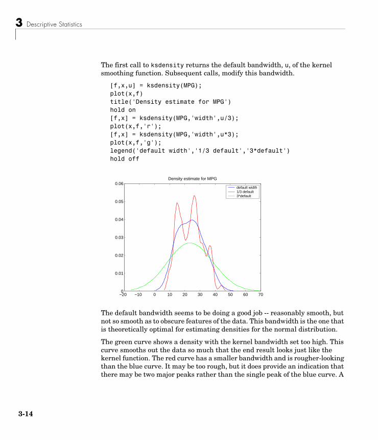
3 Descriptive Statistics
3-1
The first call to ksdensity returns the default bandwidth, u, of the kernel smoothing function. Subsequent calls, modify this bandwidth.
[f,x,u] = ksdensity(MPG);plot(x,f)title('Density estimate for MPG')hold on[f,x] = ksdensity(MPG,'width',u/3);plot(x,f,'r');[f,x] = ksdensity(MPG,'width',u*3);plot(x,f,'g');legend('default width','1/3 default','3*default')hold off
The default bandwidth seems to be doing a good job -- reasonably smooth, but not so smooth as to obscure features of the data. This bandwidth is the one that is theoretically optimal for estimating densities for the normal distribution.
The green curve shows a density with the kernel bandwidth set too high. This curve smooths out the data so much that the end result looks just like the kernel function. The red curve has a smaller bandwidth and is rougher-looking than the blue curve. It may be too rough, but it does provide an indication that there may be two major peaks rather than the single peak of the blue curve. A
−20 −10 0 10 20 30 40 50 60 700
0.01
0.02
0.03
0.04
0.05
0.06Density estimate for MPG
default width1/3 default3*default
4

Percentiles and Graphical Descriptions
reasonable choice of width might lead to a curve that is intermediate between the red and blue curves.
Kernel Smoothing FunctionYou can also specify a kernel function by supplying either the function name or a function handle. The four pre-selected functions, 'normal', 'epanechinikov', 'box', and 'triangle', are all scaled to have standard deviation equal to one, so the "bandwidth" parameter means roughly the same thing regardless of kernel function.
Using default bandwidths, we now plot the same mileage data, using each of the available kernel smoothers.
hname = {'normal' 'epanechinikov' 'box' 'triangle'};hold on;colors = {'r' 'b' 'g' 'm'};for j=1:4 [f,x] = ksdensity(MPG,'kernel',hname{j}); plot(x,f,colors{j});endlegend(hname{:});hold off
0 10 20 30 40 50 600
0.005
0.01
0.015
0.02
0.025
0.03
0.035
0.04
0.045
0.05normalepanechinikovboxtriangle
3-15

3 Descriptive Statistics
3-1
The density estimates are roughly comparable, but the box kernel produces a density that is rougher than the others.
Usefulness of Smooth Density EstimatesIn addition to the aesthetic appeal of the smooth density estimate, there are other appeals as well. While it is difficult to overlay two histograms to compare them, you can easily overlay smooth density estimates. For example, the following graph shows the MPG distributions for cars from different countries of origin.
Empirical Cumulative Distribution FunctionThe ksdensity function described in the last section produces an empirical version of a probability density function (pdf). That is, instead of selecting a density with a particular parametric form and estimating the parameters, it produces a nonparametric density estimate that tries to adapt itself to the data.
Similarly, it is possible to produce an empirical version of the cumulative distribution function (cdf). The ecdf function computes this empirical cdf. It
0 10 20 30 40 500
0.02
0.04
0.06
0.08
0.1
0.12Density estimates for MPG by Origin
USAJapanEurope
6

Percentiles and Graphical Descriptions
returns the values of a function such that represents the proportion of observations in a sample less than or equal to .
The idea behind the empirical cdf is simple. It is a function that assigns probability to each of observations in a sample. Its graph has a stair-step appearance. If a sample comes from a distribution in a parametric family (such as a normal distribution), its empirical cdf is likely to resemble the parametric distribution. If not, its empirical distribution still gives an estimate of the cdf for the distribution that generated the data.
In the following example, we generate 20 observations from a normal distribution with mean 10 and standard deviation 2. We use ecdf to calculate the empirical cdf and stairs to plot it. Then we overlay the normal distribution curve on the empirical function.
x = normrnd(10,2,20,1);[f,xf] = ecdf(x);stairs(xf,f)xx=linspace(5,15,100);yy = normcdf(xx,10,2);hold on; plot(xx,yy,'r:'); hold offlegend('Empirical cdf','Normal cdf',2)
F F x( )x
1 n⁄ n
5 10 150
0.1
0.2
0.3
0.4
0.5
0.6
0.7
0.8
0.9
1Empirical cdfNormal cdf
3-17

3 Descriptive Statistics
3-1
The empirical cdf is especially useful in survival analysis applications. In such applications the data may be censored, that is, not observed exactly. Some individuals may fail during a study, and we observe their failure time exactly. Other individuals may drop out of the study, or may not fail until after the study is complete. The ecdf function has arguments for dealing with censored data.
8

The Bootstrap
The BootstrapIn recent years the statistical literature has examined the properties of resampling as a means to acquire information about the uncertainty of statistical estimators.
The bootstrap is a procedure that involves choosing random samples with replacement from a data set and analyzing each sample the same way. Sampling with replacement means that every sample is returned to the data set after sampling. So a particular data point from the original data set could appear multiple times in a given bootstrap sample. The number of elements in each bootstrap sample equals the number of elements in the original data set. The range of sample estimates we obtain allows us to establish the uncertainty of the quantity we are estimating.
Here is an example taken from Efron and Tibshirani (1993) comparing Law School Admission Test (LSAT) scores and subsequent law school grade point average (GPA) for a sample of 15 law schools.
load lawdataplot(lsat,gpa,'+')lsline
540 560 580 600 620 640 660 6802.7
2.8
2.9
3
3.1
3.2
3.3
3.4
3.5
3-19

3 Descriptive Statistics
3-2
The least squares fit line indicates that higher LSAT scores go with higher law school GPAs. But how sure are we of this conclusion? The plot gives us some intuition but nothing quantitative.
We can calculate the correlation coefficient of the variables using the corrcoef function.
rhohat = corrcoef(lsat,gpa)
rhohat =
1.0000 0.7764 0.7764 1.0000
Now we have a number, 0.7764, describing the positive connection between LSAT and GPA, but though 0.7764 may seem large, we still do not know if it is statistically significant.
Using the bootstrp function we can resample the lsat and gpa vectors as many times as we like and consider the variation in the resulting correlation coefficients.
Here is an example.
rhos1000 = bootstrp(1000,'corrcoef',lsat,gpa);
This command resamples the lsat and gpa vectors 1000 times and computes the corrcoef function on each sample. Here is a histogram of the result.
hist(rhos1000(:,2),30)
0

The Bootstrap
Nearly all the estimates lie on the interval [0.4 1.0].
This is strong quantitative evidence that LSAT and subsequent GPA are positively correlated. Moreover, it does not require us to make any strong assumptions about the probability distribution of the correlation coefficient.
0.2 0.3 0.4 0.5 0.6 0.7 0.8 0.9 10
10
20
30
40
50
60
70
80
90
3-21

3 Descriptive Statistics
3-2
2
Introduction . . . . . . . . . . . . . . . . . . . . 4-2
One-Way Analysis of Variance (ANOVA) . . . . . . . 4-4Example: One-Way ANOVA . . . . . . . . . . . . . . 4-4Multiple Comparisons . . . . . . . . . . . . . . . . . 4-6Example: Multiple Comparisons . . . . . . . . . . . . 4-6
Two-Way Analysis of Variance (ANOVA) . . . . . . . 4-9Example: Two-Way ANOVA . . . . . . . . . . . . . . 4-10
N-Way Analysis of Variance . . . . . . . . . . . . . 4-12Example: N-Way ANOVA with Small Data Set . . . . . . 4-12Example: N-Way ANOVA with Large Data Set . . . . . . 4-14
Multiple Linear Regression . . . . . . . . . . . . . 4-18Mathematical Foundations of Multiple Linear Regression . . 4-18Example: Multiple Linear Regression . . . . . . . . . . 4-20
Quadratic Response Surface Models . . . . . . . . . 4-22Exploring Graphs of Multidimensional Polynomials . . . . 4-22
Stepwise Regression . . . . . . . . . . . . . . . . 4-24Example: Stepwise Regression . . . . . . . . . . . . . 4-24Stepwise Regression Plot . . . . . . . . . . . . . . . 4-25Stepwise Regression Diagnostics Table . . . . . . . . . . 4-25
Generalized Linear Models . . . . . . . . . . . . . 4-28Example: Generalized Linear Models . . . . . . . . . . 4-28
Robust and Nonparametric Methods . . . . . . . . . 4-32Robust Regression . . . . . . . . . . . . . . . . . . 4-32Kruskal-Wallis Test . . . . . . . . . . . . . . . . . 4-34Friedman’s Test . . . . . . . . . . . . . . . . . . . 4-34
4
Linear Models

4 Linear Models
4-2
IntroductionLinear models represent the relationship between a continuous response variable and one or more predictor variables (either continuous or categorical) in the form
where:
• y is an n-by-1 vector of observations of the response variable.
• X is the n-by-p design matrix determined by the predictors.
• β is a p-by-1 vector of parameters.
• ε is an n-by-1 vector of random disturbances, independent of each other and usually having a normal distribution.
MATLAB uses this general form of the linear model to solve a variety of specific regression and analysis of variance (ANOVA) problems. For example, for polynomial and multiple regression problems, the columns of X are predictor variable values or powers of such values. For one-way, two-way, and higher-way ANOVA models, the columns of X are dummy (or indicator) variables that encode the predictor categories. For analysis of covariance (ANOCOVA) models, X contains values of a continuous predictor and codes for a categorical predictor.
The following sections describe a number of functions for fitting various types of linear models:
• “One-Way Analysis of Variance (ANOVA)” on page 4-4
• “Two-Way Analysis of Variance (ANOVA)” on page 4-9
• “N-Way Analysis of Variance” on page 4-12
• “Multiple Linear Regression” on page 4-18
• “Quadratic Response Surface Models” on page 4-22
• “Stepwise Regression” on page 4-24
• “Generalized Linear Models” on page 4-28
• “Robust and Nonparametric Methods” on page 4-32
See the sections below for a tour of some of the related graphical tools:
y Xβ ε+=

Introduction
• “The polytool Demo” on page 11-5
• “The aoctool Demo” on page 11-10
• “The rsmdemo Demo” on page 11-19
Note See “Linear Models” on page 4-1 for information on fitting nonlinear models.
4-3

4 Linear Models
4-4
One-Way Analysis of Variance (ANOVA)The purpose of one-way ANOVA is to find out whether data from several groups have a common mean. That is, to determine whether the groups are actually different in the measured characteristic.
One-way ANOVA is a simple special case of the linear model. The one-way ANOVA form of the model is
where:
• yij is a matrix of observations in which each column represents a different group.
• α.j is a matrix whose columns are the group means. (The “dot j” notation means that α applies to all rows of the jth column. That is, the value αij is the same for all i.)
• εij is a matrix of random disturbances.
The model posits that the columns of y are a constant plus a random disturbance. You want to know if the constants are all the same.
The following sections explore one-way ANOVA in greater detail:
• “Example: One-Way ANOVA” on page 4-4
• “Multiple Comparisons” on page 4-6
Example: One-Way ANOVAThe data below comes from a study by Hogg and Ledolter (1987) of bacteria counts in shipments of milk. The columns of the matrix hogg represent different shipments. The rows are bacteria counts from cartons of milk chosen randomly from each shipment. Do some shipments have higher counts than others?
load hogghogg
hogg =
24 14 11 7 19
yij α .j εij+=

One-Way Analysis of Variance (ANOVA)
15 7 9 7 24 21 12 7 4 19 27 17 13 7 15 33 14 12 12 10 23 16 18 18 20
[p,tbl,stats] = anova1(hogg);p
p = 1.1971e-04
The standard ANOVA table has columns for the sums of squares, degrees of freedom, mean squares (SS/df), F statistic, and p-value.
You can use the F statistic to do a hypothesis test to find out if the bacteria counts are the same. anova1 returns the p-value from this hypothesis test.
In this case the p-value is about 0.0001, a very small value. This is a strong indication that the bacteria counts from the different tankers are not the same. An F statistic as extreme as the observed F would occur by chance only once in 10,000 times if the counts were truly equal.
The p-value returned by anova1 depends on assumptions about the random disturbances εij in the model equation. For the p-value to be correct, these disturbances need to be independent, normally distributed, and have constant variance. See “Robust and Nonparametric Methods” on page 4-32 for a nonparametric function that does not require a normal assumption.
You can get some graphical assurance that the means are different by looking at the box plots in the second figure window displayed by anova1.
4-5

4 Linear Models
4-6
Multiple ComparisonsSometimes you need to determine not just if there are any differences among the means, but specifically which pairs of means are significantly different. It is tempting to perform a series of t tests, one for each pair of means, but this procedure has a pitfall.
In a t test, we compute a t statistic and compare it to a critical value. The critical value is chosen so that when the means are really the same (any apparent difference is due to random chance), the probability that the t statistic will exceed the critical value is small, say 5%. When the means are different, the probability that the statistic will exceed the critical value is larger.
In this example there are five means, so there are 10 pairs of means to compare. It stands to reason that if all the means are the same, and if we have a 5% chance of incorrectly concluding that there is a difference in one pair, then the probability of making at least one incorrect conclusion among all 10 pairs is much larger than 5%.
Fortunately, there are procedures known as multiple comparison procedures that are designed to compensate for multiple tests.
Example: Multiple ComparisonsYou can perform a multiple comparison test using the multcompare function and supplying it with the stats output from anova1.
[c,m] = multcompare(stats)
c =
1 2 3 4 5
5
10
15
20
25
30
Val
ues
Column Number

One-Way Analysis of Variance (ANOVA)
1.0000 2.0000 2.4953 10.5000 18.5047 1.0000 3.0000 4.1619 12.1667 20.1714 1.0000 4.0000 6.6619 14.6667 22.6714 1.0000 5.0000 -2.0047 6.0000 14.0047 2.0000 3.0000 -6.3381 1.6667 9.6714 2.0000 4.0000 -3.8381 4.1667 12.1714 2.0000 5.0000 -12.5047 -4.5000 3.5047 3.0000 4.0000 -5.5047 2.5000 10.5047 3.0000 5.0000 -14.1714 -6.1667 1.8381 4.0000 5.0000 -16.6714 -8.6667 -0.6619
m = 23.8333 1.9273 13.3333 1.9273 11.6667 1.9273 9.1667 1.9273 17.8333 1.9273
The first output from multcompare has one row for each pair of groups, with an estimate of the difference in group means and a confidence interval for that group. For example, the second row has the values
1.0000 3.0000 4.1619 12.1667 20.1714
indicating that the mean of group 1 minus the mean of group 3 is estimated to be 12.1667, and a 95% confidence interval for this difference is [4.1619, 20.1714]. This interval does not contain 0, so we can conclude that the means of groups 1 and 3 are different.
The second output contains the mean and its standard error for each group.
It is easier to visualize the difference between group means by looking at the graph that multcompare produces.
4-7

4 Linear Models
4-8
The graph shows that group 1 is significantly different from groups 2, 3, and 4. By using the mouse to select group 4, you can determine that it is also significantly different from group 5. Other pairs are not significantly different.

Two-Way Analysis of Variance (ANOVA)
Two-Way Analysis of Variance (ANOVA)The purpose of two-way ANOVA is to find out whether data from several groups have a common mean. One-way ANOVA and two-way ANOVA differ in that the groups in two-way ANOVA have two categories of defining characteristics instead of one.
Suppose an automobile company has two factories, and each factory makes the same three models of car. It is reasonable to ask if the gas mileage in the cars varies from factory to factory as well as from model to model. We use two predictors, factory and model, to explain differences in mileage.
There could be an overall difference in mileage due to a difference in the production methods between factories. There is probably a difference in the mileage of the different models (irrespective of the factory) due to differences in design specifications. These effects are called additive.
Finally, a factory might make high mileage cars in one model (perhaps because of a superior production line), but not be different from the other factory for other models. This effect is called an interaction. It is impossible to detect an interaction unless there are duplicate observations for some combination of factory and car model.
Two-way ANOVA is a special case of the linear model. The two-way ANOVA form of the model is
where, with respect to the automobile example above:
• yijk is a matrix of gas mileage observations (with row index i, column index j, and repetition index k).
• µ is a constant matrix of the overall mean gas mileage.
• α.j is a matrix whose columns are the deviations of each car’s gas mileage (from the mean gas mileage µ) that are attributable to the car’s model. All values in a given column of α.j are identical, and the values in each row of α.j sum to 0.
• βi. is a matrix whose rows are the deviations of each car’s gas mileage (from the mean gas mileage µ) that are attributable to the car’s factory. All values in a given row of βi. are identical, and the values in each column of βi. sum to 0.
yijk µ α .j βi. γij εijk+ + + +=
4-9
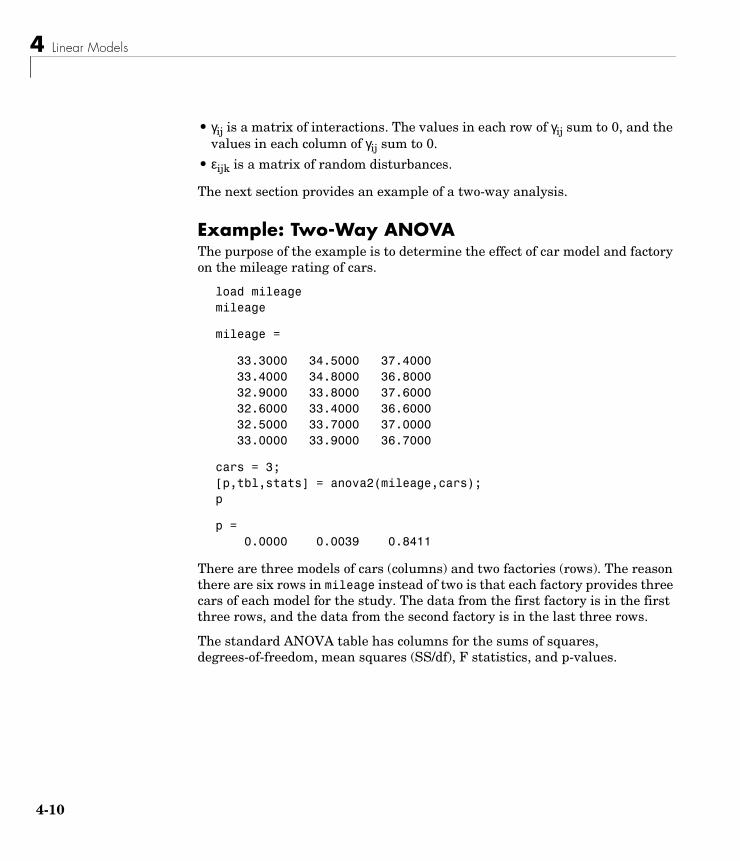
4 Linear Models
4-1
• γij is a matrix of interactions. The values in each row of γij sum to 0, and the values in each column of γij sum to 0.
• εijk is a matrix of random disturbances.
The next section provides an example of a two-way analysis.
Example: Two-Way ANOVAThe purpose of the example is to determine the effect of car model and factory on the mileage rating of cars.
load mileagemileage
mileage =
33.3000 34.5000 37.4000 33.4000 34.8000 36.8000 32.9000 33.8000 37.6000 32.6000 33.4000 36.6000 32.5000 33.7000 37.0000 33.0000 33.9000 36.7000
cars = 3;[p,tbl,stats] = anova2(mileage,cars);p
p = 0.0000 0.0039 0.8411
There are three models of cars (columns) and two factories (rows). The reason there are six rows in mileage instead of two is that each factory provides three cars of each model for the study. The data from the first factory is in the first three rows, and the data from the second factory is in the last three rows.
The standard ANOVA table has columns for the sums of squares, degrees-of-freedom, mean squares (SS/df), F statistics, and p-values.
0

Two-Way Analysis of Variance (ANOVA)
You can use the F statistics to do hypotheses tests to find out if the mileage is the same across models, factories, and model-factory pairs (after adjusting for the additive effects). anova2 returns the p-value from these tests.
The p-value for the model effect is zero to four decimal places. This is a strong indication that the mileage varies from one model to another. An F statistic as extreme as the observed F would occur by chance less than once in 10,000 times if the gas mileage were truly equal from model to model. If you used the multcompare function to perform a multiple comparison test, you would find that each pair of the three models is significantly different.
The p-value for the factory effect is 0.0039, which is also highly significant. This indicates that one factory is out-performing the other in the gas mileage of the cars it produces. The observed p-value indicates that an F statistic as extreme as the observed F would occur by chance about four out of 1000 times if the gas mileage were truly equal from factory to factory.
There does not appear to be any interaction between factories and models. The p-value, 0.8411, means that the observed result is quite likely (84 out 100 times) given that there is no interaction.
The p-values returned by anova2 depend on assumptions about the random disturbances εijk in the model equation. For the p-values to be correct these disturbances need to be independent, normally distributed, and have constant variance. See “Robust and Nonparametric Methods” on page 4-32 for nonparametric methods that do not require a normal distribution.
In addition, anova2 requires that data be balanced, which in this case means there must be the same number of cars for each combination of model and factory. The next section discusses a function that supports unbalanced data with any number of predictors.
4-11

4 Linear Models
4-1
N-Way Analysis of VarianceYou can use N-way ANOVA to determine if the means in a set of data differ when grouped by multiple factors. If they do differ, you can determine which factors or combinations of factors are associated with the difference.
N-way ANOVA is a generalization of two-way ANOVA. For three factors, the model can be written
In this notation parameters with two subscripts, such as (αβ)ij., represent the interaction effect of two factors. The parameter (αβγ)ijk represents the three-way interaction. An ANOVA model can have the full set of parameters or any subset, but conventionally it does not include complex interaction terms unless it also includes all simpler terms for those factors. For example, one would generally not include the three-way interaction without also including all two-way interactions.
The anovan function performs N-way ANOVA. Unlike the anova1 and anova2 functions, anovan does not expect data in a tabular form. Instead, it expects a vector of response measurements and a separate vector (or text array) containing the values corresponding to each factor. This input data format is more convenient than matrices when there are more than two factors or when the number of measurements per factor combination is not constant.
The following examples explore anovan in greater detail:
• “Example: N-Way ANOVA with Small Data Set” on page 4-12
• “Example: N-Way ANOVA with Large Data Set” on page 4-14
Example: N-Way ANOVA with Small Data SetConsider the following two-way example using anova2.
m = [23 15 20;27 17 63;43 3 55;41 9 90]m = 23 15 20 27 17 63 43 3 55 41 9 90
yijkl µ α .j. βi . . γ..k αβ( )ij. αγ( )i .k βγ( ).jk αβγ( )ijk ε+ + + + ijkl+ + + +=
2

N-Way Analysis of Variance
anova2(m,2)
ans = 0.0197 0.2234 0.2663
The factor information is implied by the shape of the matrix m and the number of measurements at each factor combination (2). Although anova2 does not actually require arrays of factor values, for illustrative purposes we could create them as follows.
cfactor = repmat(1:3,4,1)
cfactor =
1 2 3 1 2 3 1 2 3 1 2 3
rfactor = [ones(2,3); 2*ones(2,3)]
rfactor =
1 1 1 1 1 1 2 2 2 2 2 2
The cfactor matrix shows that each column of m represents a different level of the column factor. The rfactor matrix shows that the top two rows of m represent one level of the row factor, and bottom two rows of m represent a second level of the row factor. In other words, each value m(i,j) represents an observation at column factor level cfactor(i,j) and row factor level rfactor(i,j).
To solve the above problem with anovan, we need to reshape the matrices m, cfactor, and rfactor to be vectors.
m = m(:);cfactor = cfactor(:);rfactor = rfactor(:);
[m cfactor rfactor]
ans =
4-13

4 Linear Models
4-1
23 1 1 27 1 1 43 1 2 41 1 2 15 2 1 17 2 1 3 2 2 9 2 2 20 3 1 63 3 1 55 3 2 90 3 2
anovan(m,{cfactor rfactor},2)
ans =
0.0197 0.2234 0.2663
Example: N-Way ANOVA with Large Data SetIn the previous example we used anova2 to study a small data set measuring car mileage. Now we study a larger set of car data with mileage and other information on 406 cars made between 1970 and 1982. First we load the data set and look at the variable names.
load carbigwhos
Name Size Bytes Class
Acceleration 406x1 3248 double array Cylinders 406x1 3248 double array Displacement 406x1 3248 double array Horsepower 406x1 3248 double array MPG 406x1 3248 double array Model 406x36 29232 char array Model_Year 406x1 3248 double array Origin 406x7 5684 char array Weight 406x1 3248 double array
4

N-Way Analysis of Variance
cyl4 406x5 4060 char array org 406x7 5684 char array when 406x5 4060 char array
We will focus our attention on four variables. MPG is the number of miles per gallon for each of 406 cars (though some have missing values coded as NaN). The other three variables are factors: cyl4 (four-cylinder car or not), org (car originated in Europe, Japan, or the USA), and when (car was built early in the period, in the middle of the period, or late in the period).
First we fit the full model, requesting up to three-way interactions and Type 3 sums-of-squares.
varnames = {'Origin';'4Cyl';'MfgDate'};anovan(MPG,{org cyl4 when},3,3,varnames)
ans = 0.0000 NaN 0 0.7032 0.0001 0.2072 0.6990
Note that many terms are marked by a “#” symbol as not having full rank, and one of them has zero degrees of freedom and is missing a p-value. This can happen when there are missing factor combinations and the model has higher-order terms. In this case, the cross-tabulation below shows that there are no cars made in Europe during the early part of the period with other than four cylinders, as indicated by the 0 in table(2,1,1).
4-15

4 Linear Models
4-1
[table,factorvals] = crosstab(org,when,cyl4)
table(:,:,1) =
82 75 25 0 4 3 3 3 4
table(:,:,2) =
12 22 38 23 26 17 12 25 32
factorvals =
'USA' 'Early' 'Other' 'Europe' 'Mid' 'Four' 'Japan' 'Late' []
Consequently it is impossible to estimate the three-way interaction effects, and including the three-way interaction term in the model makes the fit singular.
Using even the limited information available in the ANOVA table, we can see that the three-way interaction has a p-value of 0.699, so it is not significant. We decide to request only two-way interactions this time.
[p,tbl,stats,termvec] = anovan(MPG,{org cyl4 when},2,3,varnames);termvec'
ans =
1 2 4 3 5 6
6

N-Way Analysis of Variance
Now all terms are estimable. The p-values for interaction term 4 (Origin*4Cyl) and interaction term 6 (4Cyl*MfgDate) are much larger than a typical cutoff value of 0.05, indicating these terms are not significant. We could choose to omit these terms and pool their effects into the error term. The output termvec variable returns a vector of codes, each of which is a bit pattern representing a term. We can omit terms from the model by deleting their entries from termvec and running anovan again, this time supplying the resulting vector as the model argument.
termvec([4 6]) = []
termvec = 1 2 4 5
anovan(MPG,{org cyl4 when},termvec,3,varnames)
Now we have a more parsimonious model indicating that the mileage of these cars seems to be related to all three factors, and that the effect of the manufacturing date depends on where the car was made.
4-17

4 Linear Models
4-1
Multiple Linear RegressionThe purpose of multiple linear regression is to establish a quantitative relationship between a group of predictor variables (the columns of X) and a response, y. This relationship is useful for:
• Understanding which predictors have the greatest effect.
• Knowing the direction of the effect (i.e., increasing x increases/decreases y).
• Using the model to predict future values of the response when only the predictors are currently known.
The following sections explain multiple linear regression in greater detail:
• “Mathematical Foundations of Multiple Linear Regression” on page 4-18
• “Example: Multiple Linear Regression” on page 4-20
Mathematical Foundations of Multiple Linear RegressionThe linear model takes its common form
where:
• y is an n-by-1 vector of observations.
• X is an n-by-p matrix of regressors.
• β is a p-by-1 vector of parameters.
• ε is an n-by-1 vector of random disturbances.
The solution to the problem is a vector, b, which estimates the unknown vector of parameters, β. The least squares solution is
This equation is useful for developing later statistical formulas, but has poor numeric properties. regress uses QR decomposition of X followed by the backslash operator to compute b. The QR decomposition is not necessary for computing b, but the matrix R is useful for computing confidence intervals.
y Xβ ε+=
b β� XTX( )1–XTy= =
8

Multiple Linear Regression
You can plug b back into the model formula to get the predicted y values at the data points.
Statisticians use a hat (circumflex) over a letter to denote an estimate of a parameter or a prediction from a model. The projection matrix H is called the hat matrix, because it puts the “hat” on y.
The residuals are the difference between the observed and predicted y values.
The residuals are useful for detecting failures in the model assumptions, since they correspond to the errors, ε, in the model equation. By assumption, these errors each have independent normal distributions with mean zero and a constant variance.
The residuals, however, are correlated and have variances that depend on the locations of the data points. It is a common practice to scale (“Studentize”) the residuals so they all have the same variance.
In the equation below, the scaled residual, ti, has a Student’s t distribution with (n-p-1) degrees of freedom
where
and:
• ti is the scaled residual for the ith data point.
• ri is the raw residual for the ith data point.
• n is the sample size.
• p is the number of parameters in the model.
y� Xb Hy= =
H X XTX( )1–XT
=
r y y�–= I H–( )y=
tiri
σ� i( ) 1 hi–----------------------------=
σ�2
i( )r 2
n p– 1–----------------------
ri2
n p– 1–( ) 1 hi–( )-----------------------------------------------–=
4-19

4 Linear Models
4-2
• hi is the ith diagonal element of H.
The left-hand side of the second equation is the estimate of the variance of the errors excluding the ith data point from the calculation.
A hypothesis test for outliers involves comparing ti with the critical values of the t distribution. If ti is large, this casts doubt on the assumption that this residual has the same variance as the others.
A confidence interval for the mean of each error is
Confidence intervals that do not include zero are equivalent to rejecting the hypothesis (at a significance probability of α) that the residual mean is zero. Such confidence intervals are good evidence that the observation is an outlier for the given model.
Example: Multiple Linear RegressionThe example comes from Chatterjee and Hadi (1986) in a paper on regression diagnostics. The data set (originally from Moore (1975)) has five predictor variables and one response.
load mooreX = [ones(size(moore,1),1) moore(:,1:5)];
Matrix X has a column of ones, and then one column of values for each of the five predictor variables. The column of ones is necessary for estimating the y-intercept of the linear model.
y = moore(:,6);[b,bint,r,rint,stats] = regress(y,X);
The y-intercept is b(1), which corresponds to the column index of the column of ones.
statsstats =
0.8107 11.9886 0.0001
ci ri t1 α
2--- ν,–
± σ� i( ) 1 hi–=
0
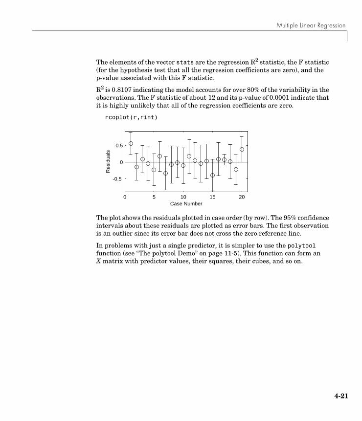
Multiple Linear Regression
The elements of the vector stats are the regression R2 statistic, the F statistic (for the hypothesis test that all the regression coefficients are zero), and the p-value associated with this F statistic.
R2 is 0.8107 indicating the model accounts for over 80% of the variability in the observations. The F statistic of about 12 and its p-value of 0.0001 indicate that it is highly unlikely that all of the regression coefficients are zero.
rcoplot(r,rint)
The plot shows the residuals plotted in case order (by row). The 95% confidence intervals about these residuals are plotted as error bars. The first observation is an outlier since its error bar does not cross the zero reference line.
In problems with just a single predictor, it is simpler to use the polytool function (see “The polytool Demo” on page 11-5). This function can form an X matrix with predictor values, their squares, their cubes, and so on.
0 5 10 15 20
-0.5
0
0.5
Res
idua
ls
Case Number
4-21

4 Linear Models
4-2
Quadratic Response Surface ModelsResponse Surface Methodology (RSM) is a tool for understanding the quantitative relationship between multiple input variables and one output variable.
Consider one output, z, as a polynomial function of two inputs, x and y. The function z = f(x,y) describes a two-dimensional surface in the space (x,y,z). Of course, you can have as many input variables as you want and the resulting surface becomes a hypersurface. You can have multiple output variables with a separate hypersurface for each one.
For three inputs (x1, x2, x3), the equation of a quadratic response surface is
It is difficult to visualize a k-dimensional surface in k+1 dimensional space for k>2. The function rstool is a graphical user interface (GUI) designed to make this visualization more intuitive, as is discussed in the next section.
Exploring Graphs of Multidimensional PolynomialsThe function rstool is useful for fitting response surface models. The purpose of rstool is larger than just fitting and prediction for polynomial models. This GUI provides an environment for exploration of the graph of a multidimensional polynomial.
You can learn about rstool by trying the commands below. The chemistry behind the data in reaction.mat deals with reaction kinetics as a function of the partial pressure of three chemical reactants: hydrogen, n-pentane, and isopentane.
load reactionrstool(reactants,rate,'quadratic',0.01,xn,yn)
You will see a “vector” of three plots. The dependent variable of all three plots is the reaction rate. The first plot has hydrogen as the independent variable. The second and third plots have n-pentane and isopentane respectively.
y b0 b1x1 b2x2 b3x3 …
b12x1x2 b13x1x3 b23x2x3 …
b11x12 b22x2
2 b33x32
+ + + +
+ + + +
+ + +
= (linear terms)
(interaction terms)
(quadratic terms)
2

Quadratic Response Surface Models
Each plot shows the fitted relationship of the reaction rate to the independent variable at a fixed value of the other two independent variables. The fixed value of each independent variable is in an editable text box below each axis. You can change the fixed value of any independent variable by either typing a new value in the box or by dragging any of the three vertical lines to a new position.
When you change the value of an independent variable, all the plots update to show the current picture at the new point in the space of the independent variables.
Note that while this example only uses three inputs (reactants) and one output (rate), rstool can accommodate an arbitrary number of inputs and outputs. Interpretability may be limited by the size of the monitor for large numbers of inputs or outputs.
The GUI also has two pop-up menus. The Export menu facilitates saving various important variables in the GUI to the base workspace. Below the Export menu there is another menu that allows you to change the order of the polynomial model from within the GUI. If you used the commands above, this menu will have the string Full Quadratic. Other choices are:
• Linear – has the constant and first order terms only.
• Pure Quadratic – includes constant, linear and squared terms.
• Interactions – includes constant, linear, and cross product terms.
The rstool GUI is used by the rsmdemo function to visualize the results of a designed experiment for studying a chemical reaction. See “The rsmdemo Demo” on page 11-19.
4-23

4 Linear Models
4-2
Stepwise Regression Stepwise regression is a technique for choosing the variables to include in a multiple regression model. Forward stepwise regression starts with no model terms. At each step it adds the most statistically significant term (the one with the highest F statistic or lowest p-value) until there are none left. Backward stepwise regression starts with all the terms in the model and removes the least significant terms until all the remaining terms are statistically significant. It is also possible to start with a subset of all the terms and then add significant terms or remove insignificant terms.
An important assumption behind the method is that some input variables in a multiple regression do not have an important explanatory effect on the response. If this assumption is true, then it is a convenient simplification to keep only the statistically significant terms in the model.
One common problem in multiple regression analysis is multicollinearity of the input variables. The input variables may be as correlated with each other as they are with the response. If this is the case, the presence of one input variable in the model may mask the effect of another input. Stepwise regression used as a canned procedure is a dangerous tool because the resulting model may include different variables depending on the choice of starting model and inclusion strategy.
The following example explores an interactive tool for stepwise regression.
Example: Stepwise RegressionThe Statistics Toolbox provides an interactive graphical user interface (GUI) to make comparison of competing models more understandable. You can explore the GUI using the Hald (1960) data set. Here are the commands to get started.
load haldstepwise(ingredients,heat)
The Hald data come from a study of the heat of reaction of various cement mixtures. There are four components in each mixture, and the amount of heat produced depends on the amount of each ingredient in the mixture.
The interface consists of three interactively linked figure windows. Two of these are discussed in the following sections:
• “Stepwise Regression Plot” on page 4-25
4
Stepwise Regression
• “Stepwise Regression Diagnostics Table” on page 4-25
All three windows have hot regions. When your mouse is above one of these regions, the pointer changes from an arrow to a circle. Clicking on this point initiates some activity in the interface.
Stepwise Regression PlotThis plot shows the regression coefficient and confidence interval for every term (in or out of the model). The green lines represent terms in the model while red lines indicate terms that are not currently in the model.
Statistically significant terms are solid lines. Dotted lines show that the fitted coefficient is not significantly different from zero.
Clicking on a line in this plot toggles its state. That is, a term currently in the model (green line) is removed (turns red), and a term currently not in the model (red line) is added (turns green).
The coefficient for a term out of the model is the coefficient resulting from adding that term to the current model.
Scale InputsPressing this button centers and normalizes the columns of the input matrix to have a standard deviation of one.
ExportThis pop-up menu allows you to export variables from the stepwise function to the base workspace.
CloseThe Close button removes all the figure windows.
Stepwise Regression Diagnostics TableThis table is a quantitative view of the information in the Stepwise Regression Plot. The table shows the Hald model with the second and third terms removed.
4-25
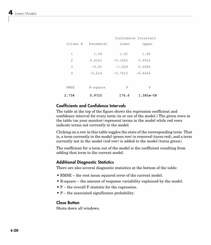
4 Linear Models
4-2
Coefficients and Confidence IntervalsThe table at the top of the figure shows the regression coefficient and confidence interval for every term (in or out of the model.) The green rows in the table (on your monitor) represent terms in the model while red rows indicate terms not currently in the model.
Clicking on a row in this table toggles the state of the corresponding term. That is, a term currently in the model (green row) is removed (turns red), and a term currently not in the model (red row) is added to the model (turns green).
The coefficient for a term out of the model is the coefficient resulting from adding that term to the current model.
Additional Diagnostic StatisticsThere are also several diagnostic statistics at the bottom of the table:
• RMSE – the root mean squared error of the current model.
• R-square – the amount of response variability explained by the model.
• F – the overall F statistic for the regression.
• P – the associated significance probability.
Close ButtonShuts down all windows.
Confidence Intervals
Column #
RMSE
Parameter
R-square
Lower
F
Upper
P
1 1.44 1.02 1.86
2.734 0.9725 176.6 1.581e-08
2 0.4161 -0.1602 0.9924
2.734 0.9725 176.6 1.581e-08
3 -0.41 -1.029 0.2086
2.734 0.9725 176.6 1.581e-08
4 -0.614 -0.7615 -0.4664
2.734 0.9725 176.6 1.581e-08
6

Stepwise Regression
Help ButtonActivates online help.
Stepwise HistoryThis plot shows the RMSE and a confidence interval for every model generated in the course of the interactive use of the other windows.
Recreating a Previous ModelClicking on one of these lines recreates the current model at that point in the analysis using a new set of windows. You can thus compare the two candidate models directly.
4-27
4 Linear Models
4-2
Generalized Linear ModelsSo far, the functions in this section have dealt with models that have a linear relationship between the response and one or more predictors. Sometimes you may have a nonlinear relationship instead. To fit nonlinear models you can use the functions described in “Nonlinear Regression Models” on page 5-1.
There are some nonlinear models, known as generalized linear models, that you can fit using simpler linear methods. To understand generalized linear models, first let’s review the linear models we have seen so far. Each of these models has the following three characteristics:
• The response has a normal distribution with mean µ.
• A coefficient vector b defines a linear combination X*b of the predictors X.
• The model equates the two as µ = X*b.
In generalized linear models, these characteristics are generalized as follows:
• The response has a distribution that may be normal, binomial, Poisson, gamma, or inverse Gaussian, with parameters including a mean µ.
• A coefficient vector b defines a linear combination X*b of the predictors X.
• A link function f(·) defines the link between the two as f(µ) = X*b.
The following example explores this in greater detail.
Example: Generalized Linear ModelsFor example, consider the following data derived from the carbig data set. We have cars of various weights, and we record the total number of cars of each weight and the number qualifying as poor-mileage cars because their miles per gallon value is below some target. (Suppose we don’t know the miles per gallon for each car, only the number passing the test.) It might be reasonable to assume that the value of the variable poor follows a binomial distribution with parameter N=total and with a p parameter that depends on the car weight. A plot shows that the proportion of poor-mileage cars follows a nonlinear S-shape.
w = [2100 2300 2500 2700 2900 3100 3300 3500 3700 3900 4100 4300]';poor = [1 2 0 3 8 8 14 17 19 15 17 21]';total = [48 42 31 34 31 21 23 23 21 16 17 21]';
8

Generalized Linear Models
[w poor total]ans = 2100 1 48 2300 2 42 2500 0 31 2700 3 34 2900 8 31 3100 8 21 3300 14 23 3500 17 23 3700 19 21 3900 15 16 4100 17 17 4300 21 21
plot(w,poor./total,'x')
This shape is typical of graphs of proportions, as they have natural boundaries at 0.0 and 1.0.
A linear regression model would not produce a satisfactory fit to this graph. Not only would the fitted line not follow the data points, it would produce invalid proportions less than 0 for light cars, and higher than 1 for heavy cars.
2000 2500 3000 3500 4000 45000
0.1
0.2
0.3
0.4
0.5
0.6
0.7
0.8
0.9
1
4-29

4 Linear Models
4-3
There is a class of regression models for dealing with proportion data. The logistic model is one such model. It defines the relationship between proportion p and weight w to be
Is this a good model for our data? It would be helpful to graph the data on this scale, to see if the relationship appears linear. However, some of our proportions are 0 and 1, so we cannot explicitly evaluate the left-hand-side of the equation. A useful trick is to compute adjusted proportions by adding small increments to the poor and total values — say a half observation to poor and a full observation to total. This keeps the proportions within range. A graph now shows a more nearly linear relationship.
padj = (poor+.5) ./ (total+1);plot(w,log(padj./(1-padj)),'x')
We can use the glmfit function to fit this logistic model.
b = glmfit(w,[poor total],'binomial')
b = -13.3801 0.0042
p1 p–------------ log b1 b2w+=
2000 2500 3000 3500 4000 4500−5
−4
−3
−2
−1
0
1
2
3
4
0

Generalized Linear Models
To use these coefficients to compute a fitted proportion, we have to invert the logistic relationship. Some simple algebra shows that the logistic equation can also be written as
Fortunately, the function glmval can decode this link function to compute the fitted values. Using this function we can graph fitted proportions for a range of car weights, and superimpose this curve on the original scatter plot.
x = 2100:100:4500;y = glmval(b,x, logit );plot(w,poor./total,'x',x,y,'r-')
Generalized linear models can fit a variety of distributions with a variety of relationships between the distribution parameters and the predictors. A full description is beyond the scope of this document. For more information see Dobson (1990), or McCullagh and Nelder (1990). Also see the reference material for glmfit.
p 11 b– 1 b2w–( )exp+---------------------------------------------------=
2000 2500 3000 3500 4000 45000
0.1
0.2
0.3
0.4
0.5
0.6
0.7
0.8
0.9
1
4-31

4 Linear Models
4-3
Robust and Nonparametric MethodsAs mentioned in the previous sections, regression and analysis of variance procedures depend on certain assumptions, such as a normal distribution for the error term. Sometimes such an assumption is not warranted. For example, if the distribution of the errors is asymmetric or prone to extreme outliers, that is a violation of the assumption of normal errors.
The Statistics Toolbox has a robust regression function that is useful when there may be outliers. Robust methods are designed to be relatively insensitive to large changes in a small part of the data.
The Statistics Toolbox also has nonparametric versions of the one-way and two-way analysis of variance functions. Unlike classical tests, nonparametric tests make only mild assumptions about the data, and are appropriate when the distribution of the data is not normal. On the other hand, they are less powerful than classical methods for normally distributed data.
The following sections describe the robust regression and nonparametric functions in greater detail:
• “Robust Regression” on page 4-32
• “Kruskal-Wallis Test” on page 4-34
• “Friedman’s Test” on page 4-34
Both of the nonparametric functions described here can return a stats structure that you can use as input to the multcompare function to perform multiple comparisons.
Note See for information on another type of nonparametric regression.
Robust RegressionIn “Example: Multiple Linear Regression” on page 4-20 we found an outlier when we used ordinary least squares regression to model a response as a function of five predictors. How did that outlier affect the results?
Let’s estimate the coefficients using the robustfit function.
load moore
2

Robust and Nonparametric Methods
x = moore(:,1:5);y = moore(:,6);[br,statsr] = robustfit(x,y);brbr = -1.7742 0.0000 0.0009 0.0002 0.0062 0.0001
Compare these estimates to those we obtained from the regress function.
bb = -2.1561 -0.0000 0.0013 0.0001 0.0079 0.0001
To understand why the two differ, it is helpful to look at the weight variable from the robust fit. It measures how much weight was given to each point during the fit. In this case, the first point had a very low weight so it was effectively ignored.
statsr.w'
ans =
Columns 1 through 7 0.0577 0.9977 0.9776 0.9455 0.9687 0.8734 0.9177 Columns 8 through 14 0.9990 0.9653 0.9679 0.9768 0.9882 0.9998 0.9979 Columns 15 through 20 0.8185 0.9757 0.9875 0.9991 0.9021 0.6953
For another example illustrating robust fitting, see “The robustdemo Demo” on page 11-22.
4-33

4 Linear Models
4-3
Kruskal-Wallis TestIn “One-Way Analysis of Variance (ANOVA)” on page 4-4 we used one-way analysis of variance to determine if the bacteria counts of milk varied from shipment to shipment. Our one-way analysis rested on the assumption that the measurements were independent, and that each had a normal distribution with a common variance and with a mean that was constant in each column. We concluded that the column means were not all the same. Let’s repeat that analysis using a nonparametric procedure.
The Kruskal-Wallis test is a nonparametric version of one-way analysis of variance. The assumption behind this test is that the measurements come from a continuous distribution, but not necessarily a normal distribution. The test is based on an analysis of variance using the ranks of the data values, not the data values themselves. Output includes a table similar to an anova table, and a box plot.
We can run this test as follows.
p = kruskalwallis(hogg)p = 0.0020
The low p-value means the Kruskal-Wallis test results agree with the one-way analysis of variance results.
Friedman’s TestIn “Two-Way Analysis of Variance (ANOVA)” on page 4-9 we used two-way analysis of variance to study the effect of car model and factory on car mileage. We tested whether either of these factors had a significant effect on mileage, and whether there was an interaction between these factors. We concluded that there was no interaction, but that each individual factor had a significant effect. Now we will see if a nonparametric analysis will lead to the same conclusion.
Friedman’s test is a nonparametric test for data having a two-way layout (data grouped by two categorical factors). Unlike two-way analysis of variance, Friedman’s test does not treat the two factors symmetrically and it does not test for an interaction between them. Instead, it is a test for whether the columns are different after adjusting for possible row differences. The test is based on an analysis of variance using the ranks of the data across categories of the row factor. Output includes a table similar to an anova table.
4

Robust and Nonparametric Methods
We can run Friedman’s test as follows.
p = friedman(mileage, 3)
ans =
7.4659e-004
Recall the classical analysis of variance gave a p-value to test column effects, row effects, and interaction effects. This p-value is for column effects. Using either this p-value or the p-value from ANOVA (p < 0.0001), we conclude that there are significant column effects.
In order to test for row effects, we need to rearrange the data to swap the roles of the rows in columns. For a data matrix x with no replications, we could simply transpose the data and type
p = friedman(x )
With replicated data it is slightly more complicated. A simple way is to transform the matrix into a three-dimensional array with the first dimension representing the replicates, swapping the other two dimensions, and restoring the two-dimensional shape.
x = reshape(mileage, [3 2 3]);x = permute(x, [1 3 2]);x = reshape(x, [9 2])x = 33.3000 32.6000 33.4000 32.5000 32.9000 33.0000 34.5000 33.4000 34.8000 33.7000 33.8000 33.9000 37.4000 36.6000 36.8000 37.0000 37.6000 36.7000
friedman(x, 3)
ans =
0.0082
4-35

4 Linear Models
4-3
Again, the conclusion is similar to the conclusion from the classical analysis of variance. Both this p-value and the one from ANOVA (p = 0.0039) lead us to conclude there are significant row effects.
You cannot use Friedman’s test to test for interactions between the row and column factors.
6

Introduction . . . . . . . . . . . . . . . . . . . . 5-2
Nonlinear Least Squares . . . . . . . . . . . . . . 5-3Example: Nonlinear Modeling . . . . . . . . . . . . . 5-3An Interactive GUI for Nonlinear Fitting and Prediction . . 5-7
Regression and Classification Trees . . . . . . . . . 5-8
5
Nonlinear Regression Models
5 Nonlinear Regression Models
5-2
IntroductionNot all relationships are well described by a linear regression model. The Statistics Toolbox provides two nonlinear regression techniques that may be preferable to linear regression in some cases.
• “Nonlinear Least Squares” on page 5-3 fits a model that has a known parametric form but unknown parameter values.
• “Regression and Classification Trees” on page 5-8 approximates a regression relationship using a decision tree. Such a tree seeks to partition the data set into regions, using values of the predictor variables, so that the response variables are roughly constant in each region.

Nonlinear Least Squares
Nonlinear Least SquaresResponse Surface Methodology (RSM) is an empirical modeling approach using polynomials as local approximations to the true input/output relationship. This empirical approach is often adequate for process improvement in an industrial setting.
In scientific applications there is usually relevant theory that allows us to make a mechanistic model. Often such models are nonlinear in the unknown parameters. Nonlinear models are more difficult to fit, requiring iterative methods that start with an initial guess of the unknown parameters. Each iteration alters the current guess until the algorithm converges.
The Statistics Toolbox has functions for fitting nonlinear models of the form
where:
• y is an-n by-1 vector of observations.
• f is any function of X and β.• X is an n-by-p matrix of input variables.
• β is a p-by-1 vector of unknown parameters to be estimated.
• ε is an n-by-1 vector of random disturbances.
This is explored further in the following sections:
• “Example: Nonlinear Modeling” on page 5-3
• “An Interactive GUI for Nonlinear Fitting and Prediction” on page 5-7
Example: Nonlinear ModelingThe Hougen-Watson model (Bates and Watts, [2]) for reaction kinetics is one specific example of this type. The form of the model is
where β1, β2, ..., β5 are the unknown parameters, and x1, x2, and x3 are the three input variables. The three inputs are hydrogen, n-pentane, and
y f X β,( ) ε+=
rateβ1 x2⋅ x3 β5⁄–
1 β2 x1⋅ β3 x2⋅ β4 x3⋅+ + +------------------------------------------------------------------------=
5-3

5 Nonlinear Regression Models
5-4
isopentane. It is easy to see that the parameters do not enter the model linearly.
The file reaction.mat contains simulated data from this reaction.
load reactionwhoYour variables are:
beta rate xn model reactants yn
The variables are as follows:
• rate is a 13-by-1 vector of observed reaction rates.
• reactants is a 13-by-3 matrix of reactants.
• beta is 5-by-1 vector of initial parameter estimates.
• model is a string containing the nonlinear function name.
• xn is a string matrix of the names of the reactants.
• yn is a string containing the name of the response.
The data and model are explored further in the following sections:
• “Fitting the Hougen-Watson Model” on page 5-4
• “Confidence Intervals on the Parameter Estimates” on page 5-6
• “Confidence Intervals on the Predicted Responses” on page 5-6
• “An Interactive GUI for Nonlinear Fitting and Prediction” on page 5-7
Fitting the Hougen-Watson ModelThe Statistics Toolbox provides the function nlinfit for finding parameter estimates in nonlinear modeling. nlinfit returns the least squares parameter estimates. That is, it finds the parameters that minimize the sum of the squared differences between the observed responses and their fitted values. It uses the Gauss-Newton algorithm with Levenberg-Marquardt modifications for global convergence.
nlinfit requires the input data, the responses, and an initial guess of the unknown parameters. You must also supply the name of a function that takes the input data and the current parameter estimate and returns the predicted responses. In MATLAB terminology, nlinfit is called a “function” function.

Nonlinear Least Squares
Here is the hougen function.
function yhat = hougen(beta,x)%HOUGEN Hougen-Watson model for reaction kinetics.% YHAT = HOUGEN(BETA,X) gives the predicted values of the% reaction rate, YHAT, as a function of the vector of % parameters, BETA, and the matrix of data, X.% BETA must have five elements and X must have three% columns.%% The model form is:% y = (b1*x2 - x3/b5)./(1+b2*x1+b3*x2+b4*x3)
b1 = beta(1);b2 = beta(2);b3 = beta(3);b4 = beta(4);b5 = beta(5);
x1 = x(:,1);x2 = x(:,2);x3 = x(:,3);
yhat = (b1*x2 - x3/b5)./(1+b2*x1+b3*x2+b4*x3);
To fit the reaction data, call the function nlinfit.
load reactionbetahat = nlinfit(reactants,rate,'hougen',beta)
betahat =
1.2526 0.0628 0.0400 0.1124 1.1914
nlinfit has two optional outputs. They are the residuals and Jacobian matrix at the solution. The residuals are the differences between the observed and fitted responses. The Jacobian matrix is the direct analog of the matrix X in the standard linear regression model.
5-5

5 Nonlinear Regression Models
5-6
These outputs are useful for obtaining confidence intervals on the parameter estimates and predicted responses.
Confidence Intervals on the Parameter EstimatesUsing nlparci, form 95% confidence intervals on the parameter estimates, betahat, from the reaction kinetics example.
[betahat,resid,J] = nlinfit(reactants,rate,'hougen',beta);betaci = nlparci(betahat,resid,J)
betaci =
-0.7467 3.2519 -0.0377 0.1632 -0.0312 0.1113 -0.0609 0.2857 -0.7381 3.1208
Confidence Intervals on the Predicted ResponsesUsing nlpredci, form 95% confidence intervals on the predicted responses from the reaction kinetics example.
[yhat,delta] = nlpredci('hougen',reactants,betahat,resid,J);opd = [rate yhat delta]
opd =
8.5500 8.2937 0.9178 3.7900 3.8584 0.7244 4.8200 4.7950 0.8267 0.0200 -0.0725 0.4775 2.7500 2.5687 0.4987 14.3900 14.2227 0.9666 2.5400 2.4393 0.9247 4.3500 3.9360 0.7327 13.0000 12.9440 0.7210 8.5000 8.2670 0.9459 0.0500 -0.1437 0.9537 11.3200 11.3484 0.9228 3.1300 3.3145 0.8418

Nonlinear Least Squares
Matrix opd has the observed rates in column 1 and the predictions in column 2. The 95% confidence interval is column 2±column 3. These are simultaneous confidence intervals for the estimated function at each input value. They are not intervals for new response observations at those inputs, even though most of the confidence intervals do contain the original observations.
An Interactive GUI for Nonlinear Fitting and PredictionThe function nlintool for nonlinear models is a direct analog of rstool for polynomial models. nlintool calls nlinfit and requires the same inputs.
The purpose of nlintool is larger than just fitting and prediction for nonlinear models. This GUI provides an environment for exploration of the graph of a multidimensional nonlinear function.
If you have already loaded reaction.mat, you can start nlintool.
nlintool(reactants,rate,'hougen',beta,0.01,xn,yn)
You will see a “vector” of three plots. The dependent variable of all three plots is the reaction rate. The first plot has hydrogen as the independent variable. The second and third plots have n-pentane and isopentane respectively.
Each plot shows the fitted relationship of the reaction rate to the independent variable at a fixed value of the other two independent variables. The fixed value of each independent variable is in an editable text box below each axis. You can change the fixed value of any independent variable by either typing a new value in the box or by dragging any of the three vertical lines to a new position.
When you change the value of an independent variable, all the plots update to show the current picture at the new point in the space of the independent variables.
Note that while this example only uses three reactants, nlintool can accommodate an arbitrary number of independent variables. Interpretability may be limited by the size of the monitor for large numbers of inputs.
5-7

5 Nonlinear Regression Models
5-8
Regression and Classification TreesIn nonlinear least squares we suppose that we know the form of the relationship between the response and predictor. Suppose instead that we don't know that relationship, and also that we are unwilling to assume the relationship can be well approximated by a linear model. We need a more nonparametric type of regression fitting approach. One such approach is based on "trees."
A regression tree is a sequence of questions that can be answered as yes or no, plus a set of fitted response values. Each question asks whether a predictor satisfies a given condition. Predictors can be continuous or discrete. Depending on the answers to one question, we either proceed to another question or we arrive at a fitted response value.
In this example we fit a regression tree to variables from the carsmall data set. We use the same variables as in the Analysis of Covariance example (see “The aoctool Demo” on page 11-10), so we have one continuous predictor (car weight) and one discrete predictor (model year).
Our goal is to model mileage (MPG) as a function of car weight and model year. First we load the data and then create a matrix x of predictor values and a vector y of response variables. We fit a regression tree, specifying the model year column as a categorical variable. In this data set there are cars from the three different model years 1970, 1976, and 1982.
load carsmallx = [Weight,Model_Year];y = MPG;t = treefit(x,y,'catidx',2);treedisp(t,'name',{'Wt' 'Yr'});

Regression and Classification Trees
Now we want to use this model to determine the predicted mileage for a car weighing 3000 pounds from model year 1982. Start at the top node. The weight is less than the cutoff value of 3085.5, so we take the left branch. The model year is not 1970 or 1976, so we take the right branch. We continue moving down the tree until we arrive at a terminal node that gives the predicted value. In this case, the predicted value is 38 miles per gallon. We can use the treeval function to find the fitted value for any set of predictor values.
treeval(t,[3000 82])
ans = 38
With a tree like this one having many branches, there is a danger that it fits the current data set well but would not do a good job at predicting new values. Some of its lower branches may be strongly affected by outliers and other
5-9

5 Nonlinear Regression Models
5-1
artifacts of the current data set. If possible we would prefer to find a simpler tree that avoids this problem of over-fitting.
We'll estimate the best tree size by cross validation. First we compute a "resubstitution" estimate of the error variance for this tree and a sequence of simpler trees and plot it as the lower (blue) line in the figure. This estimate probably under-estimates the true error variance. Then we compute a "cross-validation" estimate of the same quantity and plot it as the upper (red) line. The cross-validation procedure also provides us with an estimate of the pruning level, best, needed to achieve the best tree size.
[c,s,ntn] = treetest(t,'resub');[c2,s2,n2,best] = treetest(t,'cross',x,y);plot(ntn,c,'b-', n2,c2,'r-', n2(best+1),c2(best+1),'mo');xlabel('Number of terminal nodes')ylabel('Residual variance')legend('Resubstitution error','Cross-validation error','Estimated best tree size')best
best = 10
0 5 10 15 200
10
20
30
40
50
60
70
Number of terminal nodes
Res
idua
l var
ianc
e
Resubstitution errorCross−validation errorEstimated best tree size
0

Regression and Classification Trees
The best tree is the one that has a residual variance that is no more than one standard error above the minimum value along the cross-validation line. In this case the variance is just over 14. The output best takes on values starting with 0 (representing no pruning), so we need to add 1 to use it as an index into the other output arguments.
c2(best+1)ans = 14.3440
Use the output best to create a smaller tree that is pruned to our estimated best size.
t0 = treeprune(t,'level',best);treedisp(t0,'name',{'Wt' 'Yr'})
Now plot the original data and overlay the fitted values that we get using this tree. Notice that this tree does not distinguish between cars from 1970 or 1976, so we'll create a vector yold containing fitted values for 1976 and another ynew for year 1982. Cars from 1970 have the same fitted values as those from 1976.
5-11

5 Nonlinear Regression Models
5-1
xx = (1500:20:5000)';ynew = treeval(t0,[xx 82*ones(size(xx))]);yold = treeval(t0,[xx 76*ones(size(xx))]);gscatter(Weight,MPG,Model_Year,'rgb','osx');hold on; plot(xx,yold,'b:', xx,ynew,'r--'); hold off
The tree functions (treedisp, treefit, treeprune, treetest, and treeval) can also accept a categorical response variable. In that case, the fitted value from the tree is the category with the highest predicted probability for the range of predictor values falling in a given node. The Statistics Toolbox demo entitled Classification of Fisher's Iris Data shows how to use decision trees for classification.
1500 2000 2500 3000 3500 4000 4500 50005
10
15
20
25
30
35
40
45
Weight
MP
G707682
2

Introduction . . . . . . . . . . . . . . . . . . . . 6-2
Hypothesis Test Terminology . . . . . . . . . . . . 6-3
Hypothesis Test Assumptions . . . . . . . . . . . . 6-4
Example: Hypothesis Testing . . . . . . . . . . . . 6-5
Available Hypothesis Tests . . . . . . . . . . . . . 6-9
6
Hypothesis Tests

6 Hypothesis Tests
6-2
IntroductionA hypothesis test is a procedure for determining if an assertion about a characteristic of a population is reasonable.
For example, suppose that someone says that the average price of a gallon of regular unleaded gas in Massachusetts is $1.15. How would you decide whether this statement is true? You could try to find out what every gas station in the state was charging and how many gallons they were selling at that price. That approach might be definitive, but it could end up costing more than the information is worth.
A simpler approach is to find out the price of gas at a small number of randomly chosen stations around the state and compare the average price to $1.15.
Of course, the average price you get will probably not be exactly $1.15 due to variability in price from one station to the next. Suppose your average price was $1.18. Is this three cent difference a result of chance variability, or is the original assertion incorrect? A hypothesis test can provide an answer.
The following sections provide an overview of hypothesis testing with the Statistics Toolbox:
• “Hypothesis Test Terminology” on page 6-3
• “Hypothesis Test Assumptions” on page 6-4
• “Example: Hypothesis Testing” on page 6-5
• “Available Hypothesis Tests” on page 6-9

Hypothesis Test Terminology
Hypothesis Test TerminologyTo get started, there are some terms to define and assumptions to make:
• The null hypothesis is the original assertion. In this case the null hypothesis is that the average price of a gallon of gas is $1.15. The notation is H0: µ = 1.15.
• There are three possibilities for the alternative hypothesis. You might only be interested in the result if gas prices were actually higher. In this case, the alternative hypothesis is H1: µ > 1.15. The other possibilities are H1: µ < 1.15 and H1: µ ≠ 1.15.
• The significance level is related to the degree of certainty you require in order to reject the null hypothesis in favor of the alternative. By taking a small sample you cannot be certain about your conclusion. So you decide in advance to reject the null hypothesis if the probability of observing your sampled result is less than the significance level. For a typical significance level of 5%, the notation is α = 0.05. For this significance level, the probability of incorrectly rejecting the null hypothesis when it is actually true is 5%. If you need more protection from this error, then choose a lower value of α.
• The p-value is the probability of observing the given sample result under the assumption that the null hypothesis is true. If the p-value is less than α, then you reject the null hypothesis. For example, if α = 0.05 and the p-value is 0.03, then you reject the null hypothesis.
The converse is not true. If the p-value is greater than α, you have insufficient evidence to reject the null hypothesis.
• The outputs for many hypothesis test functions also include confidence intervals. Loosely speaking, a confidence interval is a range of values that have a chosen probability of containing the true hypothesized quantity. Suppose, in our example, 1.15 is inside a 95% confidence interval for the mean, µ. That is equivalent to being unable to reject the null hypothesis at a significance level of 0.05. Conversely if the 100(1-α) confidence interval does not contain 1.15, then you reject the null hypothesis at the α level of significance.
6-3

6 Hypothesis Tests
6-4
Hypothesis Test AssumptionsThe difference between hypothesis test procedures often arises from differences in the assumptions that the researcher is willing to make about the data sample. For example, the Z-test assumes that the data represents independent samples from the same normal distribution and that you know the standard deviation, σ. The t-test has the same assumptions except that you estimate the standard deviation using the data instead of specifying it as a known quantity.
Both tests have an associated signal-to-noise ratio
The signal is the difference between the average and the hypothesized mean. The noise is the standard deviation posited or estimated.
If the null hypothesis is true, then Z has a standard normal distribution, N(0,1). T has a Student’s t distribution with the degrees of freedom, ν, equal to one less than the number of data values.
Given the observed result for Z or T, and knowing the distribution of Z and T assuming the null hypothesis is true, it is possible to compute the probability (p-value) of observing this result. A very small p-value casts doubt on the truth of the null hypothesis. For example, suppose that the p-value was 0.001, meaning that the probability of observing the given Z or T was one in a thousand. That should make you skeptical enough about the null hypothesis that you reject it rather than believe that your result was just a lucky 999 to 1 shot.
There are also nonparametric tests that do not even require the assumption that the data come from a normal distribution. In addition, there are functions for testing whether the normal assumption is reasonable.
Z x µ–σ------------ or T x µ–
s------------==
where xxin----
i 1=
n
∑=

Example: Hypothesis Testing
Example: Hypothesis TestingThis example uses the gasoline price data in gas.mat. There are two samples of 20 observed gas prices for the months of January and February, 1993.
load gasprices = [price1 price2];
As a first step, you may want to test whether the samples from each month follow a normal distribution. As each sample is relatively small, you might choose to perform a Lilliefors test (rather than a Jarque-Bera test):
lillietest(price1)
ans =
0
lillietest(price2)
ans =
0
The result of the hypothesis test is a Boolean value that is 0 when you do not reject the null hypothesis, and 1 when you do reject that hypothesis. In each case, there is no need to reject the null hypothesis that the samples have a normal distribution.
Suppose it is historically true that the standard deviation of gas prices at gas stations around Massachusetts is four cents a gallon. The Z-test is a procedure for testing the null hypothesis that the average price of a gallon of gas in January (price1) is $1.15.
[h,pvalue,ci] = ztest(price1/100,1.15,0.04)
h = 0
pvalue =
0.8668
ci =
1.1340 1.1690
6-5

6 Hypothesis Tests
6-6
The Boolean output is h = 0, so you do not reject the null hypothesis.
The result suggests that $1.15 is reasonable. The 95% confidence interval [1.1340 1.1690] neatly brackets $1.15.
What about February? Try a t-test with price2. Now you are not assuming that you know the standard deviation in price.
[h,pvalue,ci] = ttest(price2/100,1.15)
h = 1
pvalue =
4.9517e-04
ci = 1.1675 1.2025
With the Boolean result h = 1, you can reject the null hypothesis at the default significance level, 0.05.
It looks like $1.15 is not a reasonable estimate of the gasoline price in February. The low end of the 95% confidence interval is greater than 1.15.
The function ttest2 allows you to compare the means of the two data samples.
[h,sig,ci] = ttest2(price1,price2)
h = 1
sig =
0.0083
ci =
-5.7845 -0.9155
The confidence interval (ci above) indicates that gasoline prices were between one and six cents lower in January than February.
If the two samples were not normally distributed but had similar shape, it would have been more appropriate to use the nonparametric rank sum test in

Example: Hypothesis Testing
place of the t-test. We can still use the rank sum test with normally distributed data, but it is less powerful than the t-test.
[p,h,stats] = ranksum(price1, price2)
p = 0.0092
h = 1
stats = zval: -2.6064 ranksum: 314
As might be expected, the rank sum test leads to the same conclusion but it is less sensitive to the difference between samples (higher p-value).
The box plot below gives the same conclusion graphically. Note that the notches have little, if any, overlap. Refer to “Statistical Plots” on page 8-1 for more information about box plots.
boxplot(prices,1)set(gca,'XtickLabel',str2mat('January','February'))xlabel('Month')ylabel('Prices ($0.01)')
6-7

6 Hypothesis Tests
6-8
January February
110
115
120
125
Price
s ($
0.0
1)
Month

Available Hypothesis Tests
Available Hypothesis TestsThe Statistics Toolbox has functions for performing the following tests.
Function What it Tests
jbtest Normal distribution for one sample
kstest Any specified distribution for one sample
kstest2 Equal distributions for two samples
lillietest Normal distribution for one sample
ranksum Median of two unpaired samples
signrank Median of two paired samples
signtest Median of two paired samples
ttest Mean of one normal sample
ttest2 Mean of two normal samples
ztest Mean of normal sample with known standard deviation
6-9

6 Hypothesis Tests
6-1
0
Introduction . . . . . . . . . . . . . . . . . . . . 7-2
Principal Components Analysis . . . . . . . . . . . 7-3Example: Principal Components Analysis . . . . . . . . . 7-4The Principal Components (First Output) . . . . . . . . . 7-7The Component Scores (Second Output) . . . . . . . . . 7-7The Component Variances (Third Output) . . . . . . . . 7-10Hotelling’s T2 (Fourth Output) . . . . . . . . . . . . . 7-12
Factor Analysis . . . . . . . . . . . . . . . . . . 7-13Example: Finding Common Factors Affecting Stock Prices . . 7-13Factor Rotation . . . . . . . . . . . . . . . . . . . 7-16Predicting Factor Scores . . . . . . . . . . . . . . . . 7-17Comparison of Factor Analysis and Principal Components
Analysis . . . . . . . . . . . . . . . . . . . . 7-19
Multivariate Analysis of Variance (MANOVA) . . . . . 7-20Example: Multivariate Analysis of Variance . . . . . . . . 7-20
Cluster Analysis . . . . . . . . . . . . . . . . . . 7-26Hierarchical Clustering . . . . . . . . . . . . . . . . 7-26K-Means Clustering . . . . . . . . . . . . . . . . . 7-40
Classical Multidimensional Scaling . . . . . . . . . 7-47Overview . . . . . . . . . . . . . . . . . . . . . . 7-47Reconstructing a Map from Inter-City Distances . . . . . . 7-49
7
Multivariate Statistics

7 Multivariate Statistics
7-2
IntroductionMultivariate statistics is an omnibus term for a number of different statistical methods. The defining characteristic of these methods is that they all aim to understand a data set by considering a group of variables together rather than focusing on only one variable at a time.
The Statistics Toolbox has functions for these methods:
• “Principal Components Analysis” on page 7-3
• “Factor Analysis” on page 7-13
• “Multivariate Analysis of Variance (MANOVA)” on page 7-20
• “Cluster Analysis” on page 7-26
• “Classical Multidimensional Scaling” on page 7-47

Principal Components Analysis
Principal Components AnalysisOne of the difficulties inherent in multivariate statistics is the problem of visualizing multidimensionality. In MATLAB, the plot command displays a graph of the relationship between two variables. The plot3 and surf commands display different three-dimensional views. When there are more than three variables, it stretches the imagination to visualize their relationships.
Fortunately, in data sets with many variables, groups of variables often move together. One reason for this is that more than one variable may be measuring the same driving principle governing the behavior of the system. In many systems there are only a few such driving forces. But an abundance of instrumentation allows us to measure dozens of system variables. When this happens, we can take advantage of this redundancy of information. We can simplify our problem by replacing a group of variables with a single new variable.
Principal components analysis is a quantitatively rigorous method for achieving this simplification. The method generates a new set of variables, called principal components. Each principal component is a linear combination of the original variables. All the principal components are orthogonal to each other so there is no redundant information. The principal components as a whole form an orthogonal basis for the space of the data.
There are an infinite number of ways to construct an orthogonal basis for several columns of data. What is so special about the principal component basis?
The first principal component is a single axis in space. When you project each observation on that axis, the resulting values form a new variable. And the variance of this variable is the maximum among all possible choices of the first axis.
The second principal component is another axis in space, perpendicular to the first. Projecting the observations on this axis generates another new variable. The variance of this variable is the maximum among all possible choices of this second axis.
The full set of principal components is as large as the original set of variables. But it is commonplace for the sum of the variances of the first few principal components to exceed 80% of the total variance of the original data. By
7-3

7 Multivariate Statistics
7-4
examining plots of these few new variables, researchers often develop a deeper understanding of the driving forces that generated the original data.
The function princomp is used to find the principal components. The following sections provide an example and explain the four outputs of princomp:
• “Example: Principal Components Analysis” on page 7-4
• “The Principal Components (First Output)” on page 7-7
• “The Component Scores (Second Output)” on page 7-7
• “The Component Variances (Third Output)” on page 7-10
• “Hotelling’s T2 (Fourth Output)” on page 7-12
Example: Principal Components AnalysisLet us look at a sample application that uses nine different indices of the quality of life in 329 U.S. cities. These are climate, housing, health, crime, transportation, education, arts, recreation, and economics. For each index, higher is better; so, for example, a higher index for crime means a lower crime rate.
We start by loading the data in cities.mat.
load citieswhos
Name Size Bytes Class
categories 9x14 252 char array names 329x43 28294 char array ratings 329x9 23688 double array
The whos command generates a table of information about all the variables in the workspace.
The cities data set contains three variables:
• categories, a string matrix containing the names of the indices.
• names, a string matrix containing the 329 city names.
• ratings, the data matrix with 329 rows and 9 columns.
Let’s look at the value of the categories variable.

Principal Components Analysis
categories
categories = climate housing health crime transportation education arts recreation economics
Now, let’s look at the first several rows of names variable.
first5 = names(1:5,:)first5 = Abilene, TX Akron, OH Albany, GA Albany-Troy, NY Albuquerque, NM
To get a quick impression of the ratings data, make a box plot.
boxplot(ratings,0,'+',0)set(gca,'YTicklabel',categories)
These commands generate the plot below. Note that there is substantially more variability in the ratings of the arts and housing than in the ratings of crime and climate.
7-5

7 Multivariate Statistics
7-6
Ordinarily you might also graph pairs of the original variables, but there are 36 two-variable plots. Perhaps principal components analysis can reduce the number of variables we need to consider.
Sometimes it makes sense to compute principal components for raw data. This is appropriate when all the variables are in the same units. Standardizing the data is reasonable when the variables are in different units or when the variance of the different columns is substantial (as in this case).
You can standardize the data by dividing each column by its standard deviation.
stdr = std(ratings);sr = ratings./repmat(stdr,329,1);
Now we are ready to find the principal components.
[pcs,newdata,variances,t2] = princomp(sr);
The following sections explain the four outputs from princomp:
• “The Principal Components (First Output)” on page 7-7
• “The Component Scores (Second Output)” on page 7-7
• “The Component Variances (Third Output)” on page 7-10
• “Hotelling’s T2 (Fourth Output)” on page 7-12
0 1 2 3 4 5
x 104
climate
housing
health
crime
transportation
education
arts
recreation
economics
Values
Col
umn
Num
ber

Principal Components Analysis
The Principal Components (First Output)The first output of the princomp function, pcs, contains the nine principal components. These are the linear combinations of the original variables that generate the new variables.
Let’s look at the first three principal component vectors.
p3 = pcs(:,1:3)p3 =
0.2064 0.2178 -0.6900 0.3565 0.2506 -0.2082 0.4602 -0.2995 -0.0073 0.2813 0.3553 0.1851 0.3512 -0.1796 0.1464 0.2753 -0.4834 0.2297 0.4631 -0.1948 -0.0265 0.3279 0.3845 -0.0509 0.1354 0.4713 0.6073
The largest weights in the first column (first principal component) are the third and seventh elements, corresponding to the variables health and arts. All the elements of the first principal component are the same sign, making it a weighted average of all the variables.
To show the orthogonality of the principal components, note that premultiplying them by their transpose yields the identity matrix.
I = p3'*p3I =
1.0000 -0.0000 -0.0000 -0.0000 1.0000 -0.0000 -0.0000 -0.0000 1.0000
The Component Scores (Second Output)The second output, newdata, is the data in the new coordinate system defined by the principal components. This output is the same size as the input data matrix.
A plot of the first two columns of newdata shows the ratings data projected onto the first two principal components.
7-7

7 Multivariate Statistics
7-8
plot(newdata(:,1),newdata(:,2),'+')xlabel('1st Principal Component');ylabel('2nd Principal Component');
Note the outlying points in the lower right corner.
The function gname is useful for graphically identifying a few points in a plot like this. You can call gname with a string matrix containing as many case labels as points in the plot. The string matrix names works for labeling points with the city names.
gname(names)
Move your cursor over the plot and click once near each point at the top right. As you click on each point, MATLAB labels it with the proper row from the names string matrix. When you are finished labeling points, press the Return key.
Here is the resulting plot.
−4 −2 0 2 4 6 8 10 12 14−4
−3
−2
−1
0
1
2
3
4
1st Principal Component
2nd
Prin
cipa
l Com
pone
nt

Principal Components Analysis
The labeled cities are the biggest population centers in the United States. Perhaps we should consider them as a completely separate group. If we call gname without arguments, it labels each point with its row number.
We can create an index variable containing the row numbers of all the metropolitan areas we chose.
−4 −2 0 2 4 6 8 10 12 14−4
−3
−2
−1
0
1
2
3
4
1st Principal Component
2nd
Prin
cipa
l Com
pone
nt
New York, NY
Los Angeles, Long Beach, CA
San Francisco, CA
Boston, MA
Washington, DC−MD−VA
Chicago, IL
−4 −2 0 2 4 6 8 10 12 14−4
−3
−2
−1
0
1
2
3
4
1st Principal Component
2nd
Prin
cipa
l Com
pone
nt
213
179
270
43
314
65
237
234
7-9

7 Multivariate Statistics
7-1
metro = [43 65 179 213 234 270 314];names(metro,:)
ans = Boston, MA Chicago, IL Los Angeles, Long Beach, CA New York, NY Philadelphia, PA-NJ San Francisco, CA Washington, DC-MD-VA
To remove these rows from the ratings matrix, type the following.
rsubset = ratings;nsubset = names;nsubset(metro,:) = [];rsubset(metro,:) = [];
size(rsubset)ans =
322 9
To practice, repeat the analysis using the variable rsubset as the new data matrix and nsubset as the string matrix of labels.
The Component Variances (Third Output)The third output, variances, is a vector containing the variance explained by the corresponding column of newdata.
variancesvariances =
3.4083 1.2140 1.1415 0.9209 0.7533 0.6306 0.4930
0

Principal Components Analysis
0.3180 0.1204
You can easily calculate the percent of the total variability explained by each principal component.
percent_explained = 100*variances/sum(variances)percent_explained =
37.8699 13.4886 12.6831 10.2324 8.3698 7.0062 5.4783 3.5338 1.3378
A “Scree” plot is a pareto plot of the percent variability explained by each principal component.
pareto(percent_explained)xlabel('Principal Component')ylabel('Variance Explained (%)')
1 2 3 4 5 6 70
10
20
30
40
50
60
70
80
90
100
Principal Component
Var
ianc
e E
xpla
ined
(%
)
0%
10%
20%
30%
40%
50%
60%
70%
80%
90%
100%
7-11

7 Multivariate Statistics
7-1
We can see that the first three principal components explain roughly two thirds of the total variability in the standardized ratings.
Hotelling’s T2 (Fourth Output)The last output of the princomp function, t2, is Hotelling’s T2, a statistical measure of the multivariate distance of each observation from the center of the data set. This is an analytical way to find the most extreme points in the data.
[st2, index] = sort(t2); % Sort in ascending order.st2 = flipud(st2); % Values in descending order.index = flipud(index); % Indices in descending order.
extreme = index(1)extreme =
213
names(extreme,:)ans =
New York, NY
It is not surprising that the ratings for New York are the furthest from the average U.S. town.
2

Factor Analysis
Factor AnalysisMultivariate data often includes a large number of measured variables, and sometimes those variables "overlap" in the sense that groups of them may be dependent. For example, in a decathalon, each athlete competes in 10 events, but several of them can be thought of as "speed" events, while others can be thought of as "strength" events, etc. Thus, you can think of a competitor's 10 event scores as largely dependent on a smaller set of 3 or 4 types of athletic ability.
Factor Analysis is a way to fit a model to multivariate data to estimate just this sort of interdependence. In the Factor Analysis model, the measured variables depend on a smaller number of unobserved (latent) factors. Because each factor may affect several variables in common, they are known as "common factors". Each variable is assumed to be dependent on a linear combination of the common factors, and the coefficients are known as loadings. Each measured variable also includes a component due to independent random variability, known as "specific variance" because it is specific to one variable.
Specifically, Factor Analysis assumes that the covariance matrix of your data is of the form
where is the matrix of loadings, and the elements of the diagonal matrix are the specific variances. The function factoran fits the Factor Analysis model using maximum likelihood.
This section includes these topics:
• “Example: Finding Common Factors Affecting Stock Prices” on page 7-13
• “Factor Rotation” on page 7-16
• “Predicting Factor Scores” on page 7-17
• “Comparison of Factor Analysis and Principal Components Analysis” on page 7-19
Example: Finding Common Factors Affecting Stock PricesOver the course of 100 weeks, the percent change in stock prices for ten companies has been recorded. Of the ten companies, the first four can be
σx ΛΛT Ψ+=
Λ Ψ
7-13

7 Multivariate Statistics
7-1
classified as primarily technology, the next three as financial, and last three as retail. It seems reasonable that the stock prices for companies that are in the same sector might vary together as economic conditions change. Factor Analysis can provide quantitative evidence that companies within each sector do experience similar week-to-week changes in stock price.
First load the data, then call factoran and specify a model fit with three common factors. By default, factoran would compute rotated estimates of the loadings to try and make their interpretation simpler, but for the moment, specify an unrotated solution.
load stockreturns[Loadings,specificVar,T,stats] = factoran(stocks,3,... 'rotate','none');
The first two factoran return arguments are the estimated loadings and the estimated specific variances. Each row of the loadings matrix represents one of the ten stocks, and each column corresponds to a common factor. With unrotated estimates, interpretation of the factors in this fit is difficult because most of the stocks contain fairly large coefficients for two or more factors.
LoadingsLoadings = 0.8885 0.2367 -0.2354 0.7126 0.3862 0.0034 0.3351 0.2784 -0.0211 0.3088 0.1113 -0.1905 0.6277 -0.6643 0.1478 0.4726 -0.6383 0.0133 0.1133 -0.5416 0.0322 0.6403 0.1669 0.4960 0.2363 0.5293 0.5770 0.1105 0.1680 0.5524
Note “Factor Rotation” on page 7-16 helps to simplify the structure in the loadings matrix, so that it will be easier to assign meaningful interpretations to the factors.
4

Factor Analysis
From the estimated specific variances, we can see that the model indicates that a particular stock price varies quite a lot beyond the variation due to the common factors.
specificVarspecificVar = 0.0991 0.3431 0.8097 0.8559 0.1429 0.3691 0.6928 0.3162 0.3311 0.6544
A specific variance of 1 would indicate that there is no common factor component in that variable, while a specific variance of 0 would indicate that the variable is entirely determined by common factors. These data seem to fall somewhere in between.
The p-value returned in the stats structure fails to reject the null hypothesis of three common factors, suggesting that this model provides a satisfactory explanation of the covariation in these data.
stats.pans = 0.8144
To determine if fewer than three factors can provide an acceptable fit, you can try a model with two common factors. The p-value for this second fit is highly significant, and rejects the hypothesis of two factors, indicating that the simpler model is not sufficient to explain the pattern in these data.
[Loadings2,specificVar2,T2,stats2] = factoran(stocks, 2,... 'rotate','none');stats2.pans = 3.5610e-006
7-15

7 Multivariate Statistics
7-1
Factor RotationAs the results above illustrate, the estimated loadings from an unrotated Factor Analysis fit can have a complicated structure. The goal of factor rotation is to find a parameterization in which each variable has only a small number of large loadings, i.e., is affected by a small number of factors, preferably only one. This can often make it easier to interpret what the factors represent.
If you think of each row of the loadings matrix as coordinates of a point in M-dimensional space, then each factor corresponds to a coordinate axis. Factor rotation is equivalent to rotating those axes, and computing new loadings in the rotated coordinate system. There are various ways to do this. Some methods leave the axes orthogonal, while others are oblique methods that change the angles between them. For this example, rotate the estimated loadings by using the promax criterion, a common oblique method.
[LoadingsPM,specVarPM] = factoran(stocks,3,'rotate','promax');LoadingsPMLoadingsPM = 0.9452 0.1214 -0.0617 0.7064 -0.0178 0.2058 0.3885 -0.0994 0.0975 0.4162 -0.0148 -0.1298 0.1021 0.9019 0.0768 0.0873 0.7709 -0.0821 -0.1616 0.5320 -0.0888 0.2169 0.2844 0.6635 0.0016 -0.1881 0.7849 -0.2289 0.0636 0.6475
Promax rotation has created a simpler structure in the loadings, one in which most of the stocks have a large loading on only one factor. To see this more clearly, you can plot each stock using the factor loadings as coordinates. "Simple" structure in the loadings appears in this plot as stocks that fall along one of the factor axes. Because there are three factors, it's easier to see the loadings if you make a pair of two-dimensional plots.
subplot(1,2,1); plot(LoadingsPM(:,1),LoadingsPM(:,2),'b.');text(LoadingsPM(:,1),LoadingsPM(:,2), num2str((1:10)')); line([-1 1 NaN 0 0 NaN 0 0],[0 0 NaN -1 1 NaN 0 0],... 'Color','black');
6

Factor Analysis
xlabel('Factor 1'); ylabel('Factor 2'); axis square;
subplot(1,2,2); plot(LoadingsPM(:,1),LoadingsPM(:,3),'b.');text(LoadingsPM(:,1),LoadingsPM(:,3), num2str((1:10)')); line([-1 1 NaN 0 0 NaN 0 0],[0 0 NaN -1 1 NaN 0 0],... 'Color', 'black');xlabel('Factor 1');ylabel('Factor 3');axis square;
This plot shows that promax has succeeded in rotating the factor loadings to a simpler structure. Each stock depends primarily on only one factor, and it is possible to describe each factor in terms of the stocks that it affects. Based on which companies are near which axes, you could reasonably conclude that the first factor axis represents the financial sector, the second retail, and the third technology. The original conjecture, that stocks vary primarily within sector, is apparently supported by the data.
Predicting Factor ScoresSometimes, it is useful to be able to classify an observation based on its factor scores. For example, if you accepted the three-factor model and the interpretation of the rotated factors, you might want to categorize each week in terms of how favorable it was for each of the three stock sectors, based on the data from the ten observed stocks.
−1 −0.5 0 0.5 1−1
−0.5
0
0.5
1
1 2 3 4
5 6
7
8
9
10
Factor 1
Fac
tor
2
−1 −0.5 0 0.5 1−1
−0.5
0
0.5
1
1
2 3
4 5 6 7
8 9
10
Factor 1
Fac
tor
3
7-17

7 Multivariate Statistics
7-1
Since the data in this example are the raw stock price changes, and not just their correlation matrix, you can have factoran return estimates of the value of each of the three rotated common factors for each week. You can then plot the estimated scores to see how the different stock sectors were affected during each week.
[LoadingsPM,specVarPM,TPM,stats,F] = factoran(stocks, 3,... 'rotate','promax');subplot(1,1,1); plot3(F(:,1),F(:,2),F(:,3),'b.');line([-4 4 NaN 0 0 NaN 0 0], [0 0 NaN -4 4 NaN 0 0],... [0 0 NaN 0 0 NaN -4 4], 'Color','black');xlabel('Financial Sector'); ylabel('Retail Sector'); zlabel('Technology Sector');grid on; axis square;view(-22.5, 8);
Oblique rotation often creates factors that are correlated. This plot shows some evidence of correlation between the first and third factors, and you can investigate further by computing the estimated factor correlation matrix.
−4 −2 0 2 4−5
05
−4
−3
−2
−1
0
1
2
3
4
Financial SectorRetail Sector
Tec
hnol
ogy
Sec
tor
8

Factor Analysis
inv(TPM'*TPM)ans = 1.0000 0.1559 0.4082 0.1559 1.0000 -0.0559 0.4082 -0.0559 1.0000
Comparison of Factor Analysis and Principal Components AnalysisThere is a good deal of overlap in terminology and goals between Principal Components Analysis (PCA) and Factor Analysis (FA). Much of the literature on the two methods does not distinguish between them, and some algorithms for fitting the FA model involve PCA. Both are dimension-reduction techniques, in the sense that they can be used to replace a large set of observed variables with a smaller set of new variables. However, the two methods are different in their goals and in their underlying models. Roughly speaking, you should use PCA when you simply need to summarize or approximate your data using fewer dimensions (to visualize it, for example), and you should use FA when you need an explanatory model for the correlations among your data.
7-19

7 Multivariate Statistics
7-2
Multivariate Analysis of Variance (MANOVA)We reviewed the analysis of variance technique in “One-Way Analysis of Variance (ANOVA)” on page 4-4. With this technique we can take a set of grouped data and determine whether the mean of a variable differs significantly between groups. Often we have multiple variables, and we are interested in determining whether the entire set of means is different from one group to the next. There is a multivariate version of analysis of variance that can address that problem, as illustrated in the following example.
Example: Multivariate Analysis of VarianceThe carsmall data set has measurements on a variety of car models from the years 1970, 1976, and 1982. Suppose we are interested in whether the characteristics of the cars have changed over time.
First we load the data.
load carsmallwhos
Name Size Bytes Class
Acceleration 100x1 800 double array Cylinders 100x1 800 double array Displacement 100x1 800 double array Horsepower 100x1 800 double array MPG 100x1 800 double array Model 100x36 7200 char array Model_Year 100x1 800 double array Origin 100x7 1400 char array Weight 100x1 800 double array
Four of these variables (Acceleration, Displacement, Horsepower, and MPG) are continuous measurements on individual car models. The variable Model_Year indicates the year in which the car was made. We can create a grouped plot matrix of these variables using the gplotmatrix function.
x = [MPG Horsepower Displacement Weight];gplotmatrix(x,[],Model_Year,[],'+xo')
0

Multivariate Analysis of Variance (MANOVA)
(When the second argument of gplotmatrix is empty, the function graphs the columns of the x argument against each other, and places histograms along the diagonals. The empty fourth argument produces a graph with the default colors. The fifth argument controls the symbols used to distinguish between groups.)
It appears the cars do differ from year to year. The upper right plot, for example, is a graph of MPG versus Weight. The 1982 cars appear to have higher mileage than the older cars, and they appear to weigh less on average. But as a group, are the three years significantly different from one another? The manova1 function can answer that question.
[d,p,stats] = manova1(x,Model_Year)
d = 2
p =
1.0e-006 * 0 0.1141
2000 3000 4000200 400100 20020 402000
3000
4000
100
200
300
400
10
20
30
40
50
100
150
200
707682
7-21
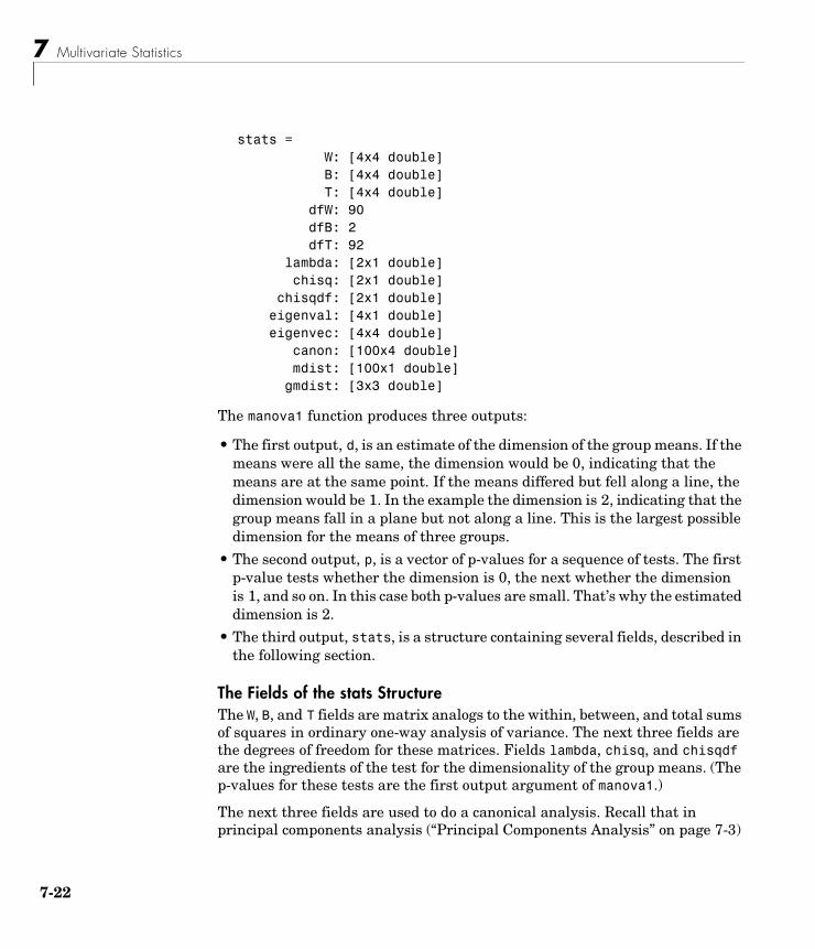
7 Multivariate Statistics
7-2
stats = W: [4x4 double] B: [4x4 double] T: [4x4 double] dfW: 90 dfB: 2 dfT: 92 lambda: [2x1 double] chisq: [2x1 double] chisqdf: [2x1 double] eigenval: [4x1 double] eigenvec: [4x4 double] canon: [100x4 double] mdist: [100x1 double] gmdist: [3x3 double]
The manova1 function produces three outputs:
• The first output, d, is an estimate of the dimension of the group means. If the means were all the same, the dimension would be 0, indicating that the means are at the same point. If the means differed but fell along a line, the dimension would be 1. In the example the dimension is 2, indicating that the group means fall in a plane but not along a line. This is the largest possible dimension for the means of three groups.
• The second output, p, is a vector of p-values for a sequence of tests. The first p-value tests whether the dimension is 0, the next whether the dimension is 1, and so on. In this case both p-values are small. That’s why the estimated dimension is 2.
• The third output, stats, is a structure containing several fields, described in the following section.
The Fields of the stats StructureThe W, B, and T fields are matrix analogs to the within, between, and total sums of squares in ordinary one-way analysis of variance. The next three fields are the degrees of freedom for these matrices. Fields lambda, chisq, and chisqdf are the ingredients of the test for the dimensionality of the group means. (The p-values for these tests are the first output argument of manova1.)
The next three fields are used to do a canonical analysis. Recall that in principal components analysis (“Principal Components Analysis” on page 7-3)
2

Multivariate Analysis of Variance (MANOVA)
we look for the combination of the original variables that has the largest possible variation. In multivariate analysis of variance, we instead look for the linear combination of the original variables that has the largest separation between groups. It is the single variable that would give the most significant result in a univariate one-way analysis of variance. Having found that combination, we next look for the combination with the second highest separation, and so on.
The eigenvec field is a matrix that defines the coefficients of the linear combinations of the original variables. The eigenval field is a vector measuring the ratio of the between-group variance to the within-group variance for the corresponding linear combination. The canon field is a matrix of the canonical variable values. Each column is a linear combination of the mean-centered original variables, using coefficients from the eigenvec matrix.
A grouped scatter plot of the first two canonical variables shows more separation between groups then a grouped scatter plot of any pair of original variables. In this example it shows three clouds of points, overlapping but with distinct centers. One point in the bottom right sits apart from the others. By using the gname function, we can see that this is the 20th point.
c1 = stats.canon(:,1);c2 = stats.canon(:,2);gscatter(c2,c1,Model_Year,[],'oxs')gname
−4 −3 −2 −1 0 1 2 3 4 5−6
−4
−2
0
2
4
6
c2
c1
20
707682
7-23

7 Multivariate Statistics
7-2
Roughly speaking, the first canonical variable, c1, separates the 1982 cars (which have high values of c1) from the older cars. The second canonical variable, c2, reveals some separation between the 1970 and 1976 cars.
The final two fields of the stats structure are Mahalanobis distances. The mdist field measures the distance from each point to its group mean. Points with large values may be outliers. In this data set, the largest outlier is the one we saw in the scatter plot, the Buick Estate station wagon. (Note that we could have supplied the model name to the gname function above if we wanted to label the point with its model name rather than its row number.)
max(stats.mdist)ans =
31.5273
find(stats.mdist == ans)ans =
20
Model(20,:)ans =
buick_estate_wagon_(sw)
The gmdist field measures the distances between each pair of group means. The following commands examine the group means and their distances:
grpstats(x, Model_Year)
ans =
1.0e+003 * 0.0177 0.1489 0.2869 3.4413 0.0216 0.1011 0.1978 3.0787 0.0317 0.0815 0.1289 2.4535
stats.gmdist
ans = 0 3.8277 11.1106 3.8277 0 6.1374 11.1106 6.1374 0
4

Multivariate Analysis of Variance (MANOVA)
As might be expected, the multivariate distance between the extreme years 1970 and 1982 (11.1) is larger than the difference between more closely spaced years (3.8 and 6.1). This is consistent with the scatter plots, where the points seem to follow a progression as the year changes from 1970 through 1976 to 1982. If we had more groups, we might have found it instructive to use the manovacluster function to draw a diagram that presents clusters of the groups, formed using the distances between their means.
7-25
7 Multivariate Statistics
7-2
Cluster AnalysisCluster analysis, also called segmentation analysis or taxonomy analysis, is a way to way to create groups of objects, or clusters, in such a way that the profiles of objects in the same cluster are very similar and the profiles of objects in different clusters are quite distinct.
Cluster analysis can be performed on many different types of data sets. For example, a data set might contain a number of observations of subjects in a study where each observation contains a set of variables.
Many different fields of study, such as engineering, zoology, medicine, linguistics, anthropology, psychology, and marketing, have contributed to the development of clustering techniques and the application of such techniques. For example, cluster analysis can help in creating "balanced" treatment and control groups for a designed study. If you find that each cluster contains roughly equal numbers of treatment and control subjects, then statistical differences found between the groups can be attributed to the experiment and not to any initial difference between the groups.
This sections explores two kinds of clustering:
• “Hierarchical Clustering” on page 7-26
• “K-Means Clustering” on page 7-40
Hierarchical ClusteringHierarchical clustering is a way to investigate grouping in your data, simultaneously over a variety of scales, by creating a cluster tree. The tree is not a single set of clusters, but rather a multi-level hierarchy, where clusters at one level are joined as clusters at the next higher level. This allows you to decide what level or scale of clustering is most appropriate in your application.
The following sections explore the hierarchical clustering features in the Statistics Toolbox:
• “Terminology and Basic Procedure” on page 7-27
• “Finding the Similarities Between Objects” on page 7-27
• “Defining the Links Between Objects” on page 7-30
• “Evaluating Cluster Formation” on page 7-32
• “Creating Clusters” on page 7-37
6

Cluster Analysis
Terminology and Basic ProcedureTo perform hierarchical cluster analysis on a data set using the Statistics Toolbox functions, follow this procedure:
1 Find the similarity or dissimilarity between every pair of objects in the data set. In this step, you calculate the distance between objects using the pdist function. The pdist function supports many different ways to compute this measurement. See “Finding the Similarities Between Objects” on page 7-27 for more information.
2 Group the objects into a binary, hierarchical cluster tree. In this step, you link together pairs of objects that are in close proximity using the linkage function. The linkage function uses the distance information generated in step 1 to determine the proximity of objects to each other. As objects are paired into binary clusters, the newly formed clusters are grouped into larger clusters until a hierarchical tree is formed. See “Defining the Links Between Objects” on page 7-30 for more information.
3 Determine where to divide the hierarchical tree into clusters. In this step, you divide the objects in the hierarchical tree into clusters using the cluster function. The cluster function can create clusters by detecting natural groupings in the hierarchical tree or by cutting off the hierarchical tree at an arbitrary point. See “Creating Clusters” on page 7-37 for more information.
The following sections provide more information about each of these steps.
Note The Statistics Toolbox includes a convenience function, clusterdata, which performs all these steps for you. You do not need to execute the pdist, linkage, or cluster functions separately. However, the clusterdata function does not give you access to the options each of the individual routines offers. For example, if you use the pdist function you can choose the distance calculation method, whereas if you use the clusterdata function you cannot.
Finding the Similarities Between ObjectsYou use the pdist function to calculate the distance between every pair of objects in a data set. For a data set made up of m objects, there are
7-27

7 Multivariate Statistics
7-2
pairs in the data set. The result of this computation is commonly known as a distance or dissimilarity matrix.
There are many ways to calculate this distance information. By default, the pdist function calculates the Euclidean distance between objects; however, you can specify one of several other options. See pdist for more information.
Note You can optionally normalize the values in the data set before calculating the distance information. In a real world data set, variables can be measured against different scales. For example, one variable can measure Intelligence Quotient (IQ) test scores and another variable can measure head circumference. These discrepancies can distort the proximity calculations. Using the zscore function, you can convert all the values in the data set to use the same proportional scale. See zscore for more information.
For example, consider a data set, X, made up of five objects where each object is a set of x,y coordinates.
• Object 1: 1, 2
• Object 2: 2.5, 4.5
• Object 3: 2, 2
• Object 4: 4, 1.5
• Object 5: 4, 2.5
You can define this data set as a matrix
X = [1 2;2.5 4.5;2 2;4 1.5;4 2.5]
and pass it to pdist. The pdist function calculates the distance between object 1 and object 2, object 1 and object 3, and so on until the distances between all the pairs have been calculated. The following figure plots these objects in a graph. The distance between object 2 and object 3 is shown to illustrate one interpretation of distance.
m m 1–( )⋅ 2⁄
8

Cluster Analysis
Returning Distance Information . The pdist function returns this distance information in a vector, Y, where each element contains the distance between a pair of objects.
Y = pdist(X)
Y =
Columns 1 through 7 2.9155 1.0000 3.0414 3.0414 2.5495 3.3541 2.5000 Columns 8 through 10 2.0616 2.0616 1.0000
To make it easier to see the relationship between the distance information generated by pdist and the objects in the original data set, you can reformat the distance vector into a matrix using the squareform function. In this matrix, element i,j corresponds to the distance between object i and object j in the original data set. In the following example, element 1,1 represents the distance between object 1 and itself (which is zero). Element 1,2 represents the distance between object 1 and object 2, and so on.
squareform(Y)
ans = 0 2.9155 1.0000 3.0414 3.0414 2.9155 0 2.5495 3.3541 2.5000 1.0000 2.5495 0 2.0616 2.0616
1 2 3 4 5
1
2
3
4
5
1
2
34
5
distance
7-29

7 Multivariate Statistics
7-3
3.0414 3.3541 2.0616 0 1.0000 3.0414 2.5000 2.0616 1.0000 0
Defining the Links Between ObjectsOnce the proximity between objects in the data set has been computed, you can determine which objects in the data set should be grouped together into clusters, using the linkage function. The linkage function takes the distance information generated by pdist and links pairs of objects that are close together into binary clusters (clusters made up of two objects). The linkage function then links these newly formed clusters to other objects to create bigger clusters until all the objects in the original data set are linked together in a hierarchical tree.
For example, given the distance vector Y generated by pdist from the sample data set of x and y coordinates, the linkage function generates a hierarchical cluster tree, returning the linkage information in a matrix, Z.
Z = linkage(Y)Z = 1.0000 3.0000 1.0000 4.0000 5.0000 1.0000 6.0000 7.0000 2.0616 8.0000 2.0000 2.5000
In this output, each row identifies a link. The first two columns identify the objects that have been linked, that is, object 1, object 2, and so on. The third column contains the distance between these objects. For the sample data set of x and y coordinates, the linkage function begins by grouping together objects 1 and 3, which have the closest proximity (distance value = 1.0000). The linkage function continues by grouping objects 4 and 5, which also have a distance value of 1.0000.
The third row indicates that the linkage function grouped together objects 6 and 7. If our original sample data set contained only five objects, what are objects 6 and 7? Object 6 is the newly formed binary cluster created by the grouping of objects 1 and 3. When the linkage function groups two objects together into a new cluster, it must assign the cluster a unique index value, starting with the value m+1, where m is the number of objects in the original data set. (Values 1 through m are already used by the original data set.) Object 7 is the index for the cluster formed by objects 4 and 5.
0

Cluster Analysis
As the final cluster, the linkage function grouped object 8, the newly formed cluster made up of objects 6 and 7, with object 2 from the original data set. The following figure graphically illustrates the way linkage groups the objects into a hierarchy of clusters.
Plotting the Cluster TreeThe hierarchical, binary cluster tree created by the linkage function is most easily understood when viewed graphically. The Statistics Toolbox includes the dendrogram function that plots this hierarchical tree information as a graph, as in the following example.
dendrogram(Z)
1 2 3 4 5
1
2
3
4
5
1
2
3
4
567
8
7-31

7 Multivariate Statistics
7-3
In the figure, the numbers along the horizontal axis represent the indices of the objects in the original data set. The links between objects are represented as upside down U-shaped lines. The height of the U indicates the distance between the objects. For example, the link representing the cluster containing objects 1 and 3 has a height of 1. For more information about creating a dendrogram diagram, see the dendrogram function reference page.
Evaluating Cluster FormationAfter linking the objects in a data set into a hierarchical cluster tree, you may want to verify that the tree represents significant similarity groupings. In addition, you may want more information about the links between the objects. The Statistics Toolbox provides functions to perform both these tasks, as described in the following sections:
• “Verifying the Cluster Tree” on page 7-32
• “Getting More Information About Cluster Links” on page 7-33
Verifying the Cluster Tree. One way to measure the validity of the cluster information generated by the linkage function is to compare it with the original proximity data generated by the pdist function. If the clustering is valid, the linking of objects in the cluster tree should have a strong correlation with the distances between objects in the distance vector. The cophenet
1 3 4 5 2
2.5
2.0
1.5
1.0
0.5
2

Cluster Analysis
function compares these two sets of values and computes their correlation, returning a value called the cophenetic correlation coefficient. The closer the value of the cophenetic correlation coefficient is to 1, the better the clustering solution.
You can use the cophenetic correlation coefficient to compare the results of clustering the same data set using different distance calculation methods or clustering algorithms.
For example, you can use the cophenet function to evaluate the clusters created for the sample data set
c = cophenet(Z,Y)c = 0.8573
where Z is the matrix output by the linkage function and Y is the distance vector output by the pdist function.
Execute pdist again on the same data set, this time specifying the City Block metric. After running the linkage function on this new pdist output, use the cophenet function to evaluate the clustering using a different distance metric.
c = cophenet(Z,Y)c =
0.9289
The cophenetic correlation coefficient shows a stronger correlation when the City Block metric is used.
Getting More Information About Cluster Links. One way to determine the natural cluster divisions in a data set is to compare the height of each link in a cluster tree with the heights of neighboring links below it in the tree.
If a link is approximately the same height as neighboring links, it indicates that there are similarities between the objects joined at this level of the hierarchy. These links are said to exhibit a high level of consistency.
If the height of a link differs from neighboring links, it indicates that there are dissimilarities between the objects at this level in the cluster tree. This link is said to be inconsistent with the links around it. In cluster analysis, inconsistent links can indicate the border of a natural division in a data set. The cluster function uses a measure of inconsistency to determine where to
7-33

7 Multivariate Statistics
7-3
divide a data set into clusters. (See “Creating Clusters” on page 7-37 for more information.)
The next section provides an example.
Example: Inconsistent Links. To illustrate, the following example creates a data set of random numbers with three deliberate natural groupings. In the dendrogram, note how the objects tend to collect into three groups. These three groups are then connected by three longer links. These longer links are inconsistent when compared with the links below them in the hierarchy.
rand('seed',3)X = [rand(10,2)+1;rand(10,2)+2;rand(10,2)+3];Y = pdist(X);Z = linkage(Y);dendrogram(Z);
0
0.1
0.2
0.3
0.4
0.5
0.6
0.7
23 25 29 30 27 28 26 24 21 22 11 12 15 13 16 18 20 14 17 19 1 2 7 3 6 8 9 10 4 5
These links show inconsistency when compared to links below them
These links show consistency
4

Cluster Analysis
The relative consistency of each link in a hierarchical cluster tree can be quantified and expressed as the inconsistency coefficient. This value compares the height of a link in a cluster hierarchy with the average height of neighboring links. If the object is consistent with those around it, it will have a low inconsistency coefficient. If the object is inconsistent with those around it, it will have a higher inconsistency coefficient.
To generate a listing of the inconsistency coefficient for each link the cluster tree, use the inconsistent function. The inconsistent function compares each link in the cluster hierarchy with adjacent links two levels below it in the cluster hierarchy. This is called the depth of the comparison. Using the inconsistent function, you can specify other depths. The objects at the bottom of the cluster tree, called leaf nodes, that have no further objects below them, have an inconsistency coefficient of zero.
For example, returning to the sample data set of x and y coordinates, we can use the inconsistent function to calculate the inconsistency values for the links created by the linkage function, described in “Defining the Links Between Objects” on page 7-30.
I = inconsistent(Z)I = 1.0000 0 1.0000 0 1.0000 0 1.0000 0 1.3539 0.8668 3.0000 0.8165 2.2808 0.3100 2.0000 0.7071
The inconsistent function returns data about the links in an (m-1)-by-4 matrix where each column provides data about the links.
In the sample output, the first row represents the link between objects 1 and 3. (This cluster is assigned the index 6 by the linkage function.) Because this a
Column Description
1 Mean of the heights of all the links included in the calculation
2 Standard deviation of all the links included in the calculation
3 Number of links included in the calculation
4 Inconsistency coefficient
7-35

7 Multivariate Statistics
7-3
leaf node, the inconsistency coefficient is zero. The second row represents the link between objects 4 and 5, also a leaf node. (This cluster is assigned the index 7 by the linkage function.)
The third row evaluates the link that connects these two leaf nodes, objects 6 and 7. (This cluster is called object 8 in the linkage output). Column three indicates that three links are considered in the calculation: the link itself and the two links directly below it in the hierarchy. Column one represents the mean of the heights of these links. The inconsistent function uses the height information output by the linkage function to calculate the mean. Column two represents the standard deviation between the links. The last column contains the inconsistency value for these links, 0.8165.
The following figure illustrates the links and heights included in this calculation.
Row four in the output matrix describes the link between object 8 and object 2. Column three indicates that two links are included in this calculation: the link itself and the link directly below it in the hierarchy. The inconsistency coefficient for this link is 0.7071.
The following figure illustrates the links and heights included in this calculation.
Link 1
Link 2
Link 3
Heights
1 3 4 5 2
2.5
2.0
1.5
1.0
0.5
Link 1
Link 2
Link 3
6

Cluster Analysis
Creating ClustersAfter you create the hierarchical tree of binary clusters, you can divide the hierarchy into larger clusters using the cluster function. The cluster function lets you create clusters in two ways, as discussed in the following sections:
• “Finding the Natural Divisions in the Data Set” on page 7-37
• “Specifying Arbitrary Clusters” on page 7-38
Finding the Natural Divisions in the Data Set. In the hierarchical cluster tree, the data set may naturally align itself into clusters. This can be particularly evident in a dendrogram diagram where groups of objects are densely packed in certain areas and not in others. The inconsistency coefficient of the links in the cluster tree can identify these points where the similarities between objects change. (See “Evaluating Cluster Formation” on page 7-32 for more information about the inconsistency coefficient.) You can use this value to determine where the cluster function draws cluster boundaries.
For example, if you use the cluster function to group the sample data set into clusters, specifying an inconsistency coefficient threshold of 0.9 as the value of the cutoff argument, the cluster function groups all the objects in the sample
1 3 4 5 2
2.5
2.0
1.5
1.0
0.5
Heights
Link 1
Link 2
7-37

7 Multivariate Statistics
7-3
data set into one cluster. In this case, none of the links in the cluster hierarchy had an inconsistency coefficient greater than 0.9.
T = cluster(Z,0.9)T = 1 1 1 1 1
The cluster function outputs a vector, T, that is the same size as the original data set. Each element in this vector contains the number of the cluster into which the corresponding object from the original data set was placed.
If you lower the inconsistency coefficient threshold to 0.8, the cluster function divides the sample data set into three separate clusters.
T = cluster(Z,0.8)T =
13122
This output indicates that objects 1 and 3 were placed in cluster 1, objects 4 and 5 were placed in cluster 2, and object 2 was placed in cluster 3.
Specifying Arbitrary Clusters. Instead of letting the cluster function create clusters determined by the natural divisions in the data set, you can specify the number of clusters you want created. In this case, the value of the cutoff argument specifies the point in the cluster hierarchy at which to create the clusters.
For example, you can specify that you want the cluster function to divide the sample data set into two clusters. In this case, the cluster function creates one cluster containing objects 1, 3, 4, and 5 and another cluster containing object 2.
T = cluster(Z,2)T =
12
1 3 4 5 2
8

Cluster Analysis
111
To help you visualize how the cluster function determines how to create these clusters, the following figure shows the dendrogram of the hierarchical cluster tree. When you specify a value of 2, the cluster function draws an imaginary horizontal line across the dendrogram that bisects two vertical lines. All the objects below the line belong to one of these two clusters.
If you specify a cutoff value of 3, the cluster function cuts off the hierarchy at a lower point, bisecting three lines.
T = cluster(Z,3)T =
13122
This time, objects 1 and 3 are grouped in a cluster, objects 4 and 5 are grouped in a cluster, and object 2 is placed into a cluster, as seen in the following figure.
2.5
2.0
1.5
1.0
0.5
cutoff = 2
7-39

7 Multivariate Statistics
7-4
K-Means ClusteringThis section gives a description and an example of using the MATLAB function for K-means clustering, kmeans.
• “Overview of K-Means Clustering” on page 7-40
• “Example: Clustering Data in Four Dimensions” on page 7-41
Overview of K-Means ClusteringK-means clustering can best be described as a partitioning method. That is, the function kmeans partitions the observations in your data into K mutually exclusive clusters, and returns a vector of indices indicating to which of the k clusters it has assigned each observation. Unlike the hierarchical clustering methods used in linkage (see “Hierarchical Clustering” on page 7-26), kmeans does not create a tree structure to describe the groupings in your data, but rather creates a single level of clusters. Another difference is that K-means clustering uses the actual observations of objects or individuals in your data, and not just their proximities. These differences often mean that kmeans is more suitable for clustering large amounts of data.
kmeans treats each observation in your data as an object having a location in space. It finds a partition in which objects within each cluster are as close to
2.5
2.0
1.5
1.0
0.5
cutoff = 3
0

Cluster Analysis
each other as possible, and as far from objects in other clusters as possible. You can choose from five different distance measures, depending on the kind of data you are clustering.
Each cluster in the partition is defined by its member objects and by its centroid, or center. The centroid for each cluster is the point to which the sum of distances from all objects in that cluster is minimized. kmeans computes cluster centroids differently for each distance measure, to minimize the sum with respect to the measure that you specify.
kmeans uses an iterative algorithm that minimizes the sum of distances from each object to its cluster centroid, over all clusters. This algorithm moves objects between clusters until the sum cannot be decreased further. The result is a set of clusters that are as compact and well-separated as possible. You can control the details of the minimization using several optional input parameters to kmeans, including ones for the initial values of the cluster centroids, and for the maximum number of iterations.
Example: Clustering Data in Four DimensionsThis example explores possible clustering in four-dimensional data by analyzing the results of partitioning the points into three, four, and five clusters.
Note Because each part of this example generates random numbers sequentially, i.e., without setting a new seed, you must perform all steps in sequence to duplicate the results shown. If you perform the steps out of sequence, the answers will be essentially the same, but the intermediate results, number of iterations, or ordering of the silhouette plots may differ. See “Random Numbers in Examples” on page 1-5 to set the correct seed.
Creating Clusters and Determining Separation. First, load some data.
load kmeansdata;size(X)
ans = 560 4
7-41

7 Multivariate Statistics
7-4
Even though these data are four-dimensional, and cannot be easily visualized, kmeans enables you to investigate if a group structure exists in them. Call kmeans with k, the desired number of clusters, equal to 3. For this example, specify the city block distance measure, and use the default starting method of initializing centroids from randomly selected data points.
idx3 = kmeans(X,3,'distance','city');
To get an idea of how well-separated the resulting clusters are, you can make a silhouette plot using the cluster indices output from kmeans. The silhouette plot displays a measure of how close each point in one cluster is to points in the neighboring clusters. This measure ranges from +1, indicating points that are very distant from neighboring clusters, through 0, indicating points that are not distinctly in one cluster or another, to -1, indicating points that are probably assigned to the wrong cluster. silhouette returns these values in its first output.
[silh3,h] = silhouette(X,idx3,'city');xlabel('Silhouette Value')ylabel('Cluster')
From the silhouette plot, you can see that most points in the third cluster have a large silhouette value, greater than 0.6, indicating that that cluster is somewhat separated from neighboring clusters. However, the second cluster
0 0.2 0.4 0.6 0.8 1
1
2
3
Silhouette Value
Clu
ster
2

Cluster Analysis
contains many points with low silhouette values, and the first contains a few points with negative values, indicating that those two clusters are not well separated.
Determining the Correct Number of Clusters. Increase the number of clusters to see if kmeans can find a better grouping of the data. This time, use the optional 'display' parameter to print information about each iteration.
idx4 = kmeans(X,4, 'dist','city', 'display','iter'); iter phase num sum 1 1 560 2897.56 2 1 53 2736.67 3 1 50 2476.78 4 1 102 1779.68 5 1 5 1771.1 6 2 0 1771.16 iterations, total sum of distances = 1771.1
Notice that the total sum of distances decreases at each iteration as kmeans reassigns points between clusters and recomputes cluster centroids. In this case, the second phase of the algorithm did not make any reassignments, indicating that the first phase reached a minimum after five iterations. In some problems, the first phase may not reach a minimum, but the second phase always will.
A silhouette plot for this solution indicates that these four clusters are better separated than the three in the previous solution.
[silh4,h] = silhouette(X,idx4,'city');xlabel('Silhouette Value')ylabel('Cluster')
7-43

7 Multivariate Statistics
7-4
A more quantitative way to compare the two solutions is to look at the average silhouette values for the two cases.
mean(silh3)ans = 0.52594
mean(silh4)ans = 0.63997
Finally, try clustering the data using five clusters.
idx5 = kmeans(X,5,'dist','city','replicates',5);[silh5,h] = silhouette(X,idx5,'city');xlabel('Silhouette Value')ylabel('Cluster')mean(silh5)ans = 0.52657
0 0.2 0.4 0.6 0.8 1
1
2
3
4
Silhouette Value
Clu
ster
4

Cluster Analysis
This silhouette plot indicates that this is probably not the right number of clusters, since two of the clusters contain points with mostly low slhouette values. Without some knowledge of how many clusters are really in the data, it is a good idea to experiment with a range of values for k.
Avoiding Local Minima. Like many other types of numerical minimizations, the solution that kmeans reaches often depends on the starting points. It is possible for kmeans to reach a local minimum, where reassigning any one point to a new cluster would increase the total sum of point-to-centroid distances, but where a better solution does exist. However, you can use the optional 'replicates' parameter to overcome that problem.
For four clusters, specify five replicates, and use the 'display' parameter to print out the final sum of distances for each of the solutions.
[idx4,cent4,sumdist] = kmeans(X,4,'dist','city',... 'display','final','replicates',5);17 iterations, total sum of distances = 2303.36 5 iterations, total sum of distances = 1771.1 6 iterations, total sum of distances = 1771.1 5 iterations, total sum of distances = 1771.1 8 iterations, total sum of distances = 2303.36
The output shows that, even for this relatively simple problem, non-global minima do exist. Each of these five replicates began from a different randomly
0 0.2 0.4 0.6 0.8 1
1
2
3
4
5
Silhouette Value
Clu
ster
7-45

7 Multivariate Statistics
7-4
selected set of initial centroids, and kmeans found two different local minima. However, the final solution that kmeans returns is the one with the lowest total sum of distances, over all replicates.
sum(sumdist)ans = 1771.1
6

Classical Multidimensional Scaling
Classical Multidimensional ScalingThese two sections demonstrate how to use the function cmdscale to perform classical multidimensional scaling.
• “Overview” on page 7-47
• “Reconstructing a Map from Inter-City Distances” on page 7-49
OverviewOne of the most important goals in visualizing data is to get a sense of how near or far points are from each other. Often, you can do this with a scatter plot. However, for some analyses, the data that you have may not be in the form of "points" at all, but rather in the form of pairwise similarities or dissimilarities between cases, observations, or subjects. Without any points, you cannot make a scatter plot.
Even if your data are in the form of points rather than pairwise distances, a scatter plot of those data may not be useful. For some kinds of data, the relevant way to measure how "near" two points are may not be their Euclidean distance. While scatter plots of the raw data make it easy to compare Euclidean distances, they are not always useful when comparing other kinds of interpoint distances, city block distance for example, or even more general dissimilarities. Also, with a large number of variables, it is very difficult to visualize distances unless the data can be represented in a small number of dimensions. Some sort of dimension reduction is usually necessary.
Multidimensional Scaling (MDS) is a set of methods that address all of these problems. MDS allows you to visualize how "near" points are to each other for many kinds of distance or dissimilarity measures, and can produce a representation of your data in a small number of dimensions. MDS does not require raw data, but only a matrix of pairwise distances or dissimilarities.
The function cmdscale performs classical (metric) multidimensional scaling, also known as Principal Coordinates Analysis. cmdscale takes as an input a matrix of interpoint distances, and creates a configuration of points. Ideally, those points are in two or three dimensions, and the Euclidean distances between them reproduce the original distance matrix. Thus, a scatter plot of the points created by cmdscale will provide a visual representation of the original distances.
7-47

7 Multivariate Statistics
7-4
A Simple ExampleAs a very simple example, you can reconstruct a set of points from only their interpoint distances. First, create some four dimensional points with a small component in their fourth coordinate, and reduce them to distances.
X = [ normrnd(0,1,10,3), normrnd(0,.1,10,1) ];D = pdist(X,'euclidean');
Next, use cmdscale to find a configuration with those interpoint distances. cmdscale accepts distances as either a square matrix, or, as in this example, in the vector upper-triangular form produced by pdist.
[Y,eigvals] = cmdscale(D);
cmdscale produces two outputs. The first output, Y, is a matrix containing the reconstructed points. The second output, eigvals, is a vector containing the sorted eigenvalues of what is often referred to as the "scalar product matrix", which, in the simplest case, is equal to Y*Y'. The relative magnitudes of those eigenvalues indicate the relative contribution of the corresponding columns of Y in reproducing the original distance matrix D with the reconstructed points.
format short g[eigvals eigvals/max(abs(eigvals))]ans = 12.623 1 4.3699 0.34618 1.9307 0.15295 0.025884 0.0020505 1.7192e-015 1.3619e-016 6.8727e-016 5.4445e-017 4.4367e-017 3.5147e-018 -9.2731e-016 -7.3461e-017 -1.327e-015 -1.0513e-016 -1.9232e-015 -1.5236e-016
If eigvals contains only positive and zero (within roundoff error) eigenvalues, then the columns of Y corresponding to the positive eigenvalues provide an exact reconstruction of D, in the sense that their interpoint Euclidean distances, computed using pdist for example, are identical (within roundoff) to the values in D.
maxerr4 = max(abs(D - pdist(Y))) % exact reconstruction
8

Classical Multidimensional Scaling
maxerr4 = 2.6645e-015
If two or three of the eigenvalues in eigvals are much larger than the rest, then the distance matrix based on the corresponding columns of Y nearly reproduces the original distance matrix D. In this sense, those columns form a lower-dimensional representation that adequately describes the data. However it is not always possible to find a good low-dimensional reconstruction.
% good reconstruction in 3Dmaxerr3 = max(abs(D - pdist(Y(:,1:3)))) maxerr3 = 0.029728
% poor reconstruction in 2Dmaxerr2 = max(abs(D - pdist(Y(:,1:2)))) maxerr2 = 0.91641
The reconstruction in three dimensions reproduces D very well, but the reconstruction in two dimensionss has errors that are the same order of magnitude as the largest values in D.
max(max(D))ans = 3.4686
Often, eigvals contains some negative eigenvalues, indicating that the distances in D cannot be reproduced exactly. That is, there may not be any configuration of points whose interpoint Euclidean distances are given by D. If the largest negative eigenvalue is small in magnitude relative to the largest positive eigenvalues, then the configuration returned by cmdscale may still reproduce D well. The following example demonstrates this.
Reconstructing a Map from Inter-City DistancesGiven only the distances between 10 US cities, cmdscale can construct a map of those cities. First, create the distance matrix and pass it to cmdscale. In this example, D is a full distance matrix: it is square, symmetric, has positive entries, and zeros on the diagonal.
7-49
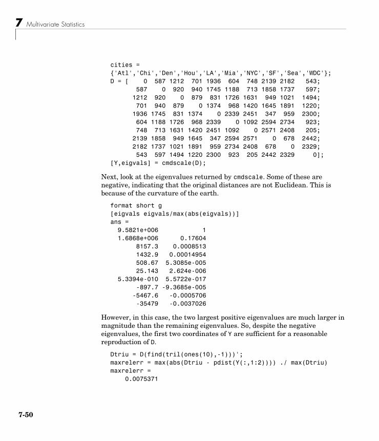
7 Multivariate Statistics
7-5
cities = {'Atl','Chi','Den','Hou','LA','Mia','NYC','SF','Sea','WDC'};D = [ 0 587 1212 701 1936 604 748 2139 2182 543; 587 0 920 940 1745 1188 713 1858 1737 597; 1212 920 0 879 831 1726 1631 949 1021 1494; 701 940 879 0 1374 968 1420 1645 1891 1220; 1936 1745 831 1374 0 2339 2451 347 959 2300; 604 1188 1726 968 2339 0 1092 2594 2734 923; 748 713 1631 1420 2451 1092 0 2571 2408 205; 2139 1858 949 1645 347 2594 2571 0 678 2442; 2182 1737 1021 1891 959 2734 2408 678 0 2329; 543 597 1494 1220 2300 923 205 2442 2329 0];[Y,eigvals] = cmdscale(D);
Next, look at the eigenvalues returned by cmdscale. Some of these are negative, indicating that the original distances are not Euclidean. This is because of the curvature of the earth.
format short g[eigvals eigvals/max(abs(eigvals))]ans = 9.5821e+006 1 1.6868e+006 0.17604 8157.3 0.0008513 1432.9 0.00014954 508.67 5.3085e-005 25.143 2.624e-006 5.3394e-010 5.5722e-017 -897.7 -9.3685e-005 -5467.6 -0.0005706 -35479 -0.0037026
However, in this case, the two largest positive eigenvalues are much larger in magnitude than the remaining eigenvalues. So, despite the negative eigenvalues, the first two coordinates of Y are sufficient for a reasonable reproduction of D.
Dtriu = D(find(tril(ones(10),-1)))';maxrelerr = max(abs(Dtriu - pdist(Y(:,1:2)))) ./ max(Dtriu)maxrelerr = 0.0075371
0

Classical Multidimensional Scaling
Here is a plot of the reconstructed city locations as a map. The orientation of the reconstruction is arbitrary: in this case, it happens to be close to, although not exactly, the correct orientation.
plot(Y(:,1),Y(:,2),'.');text(Y(:,1)+25,Y(:,2),cities);xlabel('Miles'); ylabel('Miles');
−1500 −1000 −500 0 500 1000 1500−600
−400
−200
0
200
400
600
Atl
Chi
Den
Hou
LA
Mia
NYC
SF
Sea
WDC
Miles
Mile
s
7-51

7 Multivariate Statistics
7-5
2
Introduction . . . . . . . . . . . . . . . . . . . . 8-2
Box Plots . . . . . . . . . . . . . . . . . . . . . 8-3
Distribution Plots . . . . . . . . . . . . . . . . . 8-4Normal Probability Plots . . . . . . . . . . . . . . . 8-4Quantile-Quantile Plots . . . . . . . . . . . . . . . . 8-6Weibull Probability Plots . . . . . . . . . . . . . . . 8-7Empirical Cumulative Distribution Function (CDF) . . . . 8-8
Scatter Plots . . . . . . . . . . . . . . . . . . . . 8-10
8
Statistical Plots

8 Statistical Plots
8-2
IntroductionThe Statistics Toolbox adds specialized plots to the extensive graphics capabilities of MATLAB.
• Box plots are graphs for describing data samples. They are also useful for graphic comparisons of the means of many samples (see “One-Way Analysis of Variance (ANOVA)” on page 4-4).
• Distribution plots are graphs for visualizing the distribution of one or more samples. They include normal and Weibull probability plots, quantile-quantile plots, and empirical cumulative distribution plots.
• Scatter plots are graphs for visualizing the relationship between a pair of variables or several such pairs. Grouped versions of these plots use different plotting symbols to indicate group membership. The gname function can label points on these plots with a text label or an observation number.
The plot types are described further in the following sections:
• “Box Plots” on page 8-3
• “Distribution Plots” on page 8-4
• “Scatter Plots” on page 8-10

Box Plots
Box PlotsThe graph shows an example of a notched box plot.
This plot has several graphic elements:
• The lower and upper lines of the “box” are the 25th and 75th percentiles of the sample. The distance between the top and bottom of the box is the interquartile range.
• The line in the middle of the box is the sample median. If the median is not centered in the box, that is an indication of skewness.
• The “whiskers” are lines extending above and below the box. They show the extent of the rest of the sample (unless there are outliers). Assuming no outliers, the maximum of the sample is the top of the upper whisker. The minimum of the sample is the bottom of the lower whisker. By default, an outlier is a value that is more than 1.5 times the interquartile range away from the top or bottom of the box.
• The plus sign at the top of the plot is an indication of an outlier in the data. This point may be the result of a data entry error, a poor measurement or a change in the system that generated the data.
• The notches in the box are a graphic confidence interval about the median of a sample. Box plots do not have notches by default.
A side-by-side comparison of two notched box plots is the graphical equivalent of a t-test. See “Hypothesis Tests” on page 6-1.
1
110
115
120
125V
alue
s
Column Number
8-3

8 Statistical Plots
8-4
Distribution PlotsThere are several types of plots for examining the distribution of one or more samples, as described in the following sections:
• “Normal Probability Plots” on page 8-4
• “Quantile-Quantile Plots” on page 8-6
• “Weibull Probability Plots” on page 8-7
• “Empirical Cumulative Distribution Function (CDF)” on page 8-8
Normal Probability PlotsA normal probability plot is a useful graph for assessing whether data comes from a normal distribution. Many statistical procedures make the assumption that the underlying distribution of the data is normal, so this plot can provide some assurance that the assumption of normality is not being violated, or provide an early warning of a problem with your assumptions.
This example shows a typical normal probability plot.
x = normrnd(10,1,25,1);normplot(x)
8.5 9 9.5 10 10.5 11 11.50.01 0.02
0.05
0.10
0.25
0.50
0.75
0.90
0.95
0.98 0.99
Data
Pro
babi
lity
Normal Probability Plot

Distribution Plots
The plot has three graphical elements. The plus signs show the empirical probability versus the data value for each point in the sample. The solid line connects the 25th and 75th percentiles of the data and represents a robust linear fit (i.e., insensitive to the extremes of the sample). The dashed line extends the solid line to the ends of the sample.
The scale of the y-axis is not uniform. The y-axis values are probabilities and, as such, go from zero to one. The distance between the tick marks on the y-axis matches the distance between the quantiles of a normal distribution. The quantiles are close together near the median (probability = 0.5) and stretch out symmetrically moving away from the median. Compare the vertical distance from the bottom of the plot to the probability 0.25 with the distance from 0.25 to 0.50. Similarly, compare the distance from the top of the plot to the probability 0.75 with the distance from 0.75 to 0.50.
If all the data points fall near the line, the assumption of normality is reasonable. But, if the data is nonnormal, the plus signs may follow a curve, as in the example using exponential data below.
x = exprnd(10,100,1);normplot(x)
This plot is clear evidence that the underlying distribution is not normal.
0 5 10 15 20 25 30 35 40 450.003
0.01 0.02
0.05 0.10
0.25
0.50
0.75
0.90 0.95
0.98 0.99
0.997
Data
Pro
babi
lity
Normal Probability Plot
8-5

8 Statistical Plots
8-6
Quantile-Quantile PlotsA quantile-quantile plot is useful for determining whether two samples come from the same distribution (whether normally distributed or not).
The example shows a quantile-quantile plot of two samples from a Poisson distribution.
x = poissrnd(10,50,1);y = poissrnd(5,100,1);qqplot(x,y);
Even though the parameters and sample sizes are different, the straight line relationship shows that the two samples come from the same distribution.
Like the normal probability plot, the quantile-quantile plot has three graphical elements. The pluses are the quantiles of each sample. By default the number of pluses is the number of data values in the smaller sample. The solid line joins the 25th and 75th percentiles of the samples. The dashed line extends the solid line to the extent of the sample.
The example below shows what happens when the underlying distributions are not the same.
x = normrnd(5,1,100,1);y = weibrnd(2,0.5,100,1);qqplot(x,y);
2 4 6 8 10 12 14 16 18-2
0
2
4
6
8
10
12
X Quantiles
Y Q
uant
iles

Distribution Plots
These samples clearly are not from the same distribution.
It is incorrect to interpret a linear plot as a guarantee that the two samples come from the same distribution. But, for assessing the validity of a statistical procedure that depends on the two samples coming from the same distribution (e.g., ANOVA), a linear quantile-quantile plot should be sufficient.
Weibull Probability PlotsA Weibull probability plot is a useful graph for assessing whether data comes from a Weibull distribution. Many reliability analyses make the assumption that the underlying distribution of the lifetimes is Weibull, so this plot can provide some assurance that this assumption is not being violated, or provide an early warning of a problem with your assumptions.
The scale of the y-axis is not uniform. The y-axis values are probabilities and, as such, go from zero to one. The distance between the tick marks on the y-axis matches the distance between the quantiles of a Weibull distribution.
If the data points (pluses) fall near the line, the assumption that the data comes from a Weibull distribution is reasonable.
This example shows a typical Weibull probability plot.
y = weibrnd(2,0.5,100,1);weibplot(y)
2 3 4 5 6 7 8-2
0
2
4
6
8
10
12
14
16
X Quantiles
Y Q
uant
iles
8-7

8 Statistical Plots
8-8
Empirical Cumulative Distribution Function (CDF)If you are not willing to assume that your data follows a specific probability distribution, you can use the cdfplot function to graph an empirical estimate of the cumulative distribution function (cdf). This function computes the proportion of data points less than each x value, and plots the proportion as a function of x. The y-axis scale is linear, not a probability scale for a specific distribution.
This example shows the empirical cumulative distribution function for a Weibull sample.
y = weibrnd(2,0.5,100,1);cdfplot(y)
10-4 10-2 100
0.003
0.01
0.02
0.05
0.10
0.25
0.50
0.75 0.90 0.96 0.99
Data
Pro
babi
lity
Weibull Probability Plot

Distribution Plots
The plot shows a probability function that rises steeply near x=0 and levels off for larger values. Over 80% of the observations are less than 1, with the remaining values spread over the range [1 5].
0 1 2 3 4 50
0.1
0.2
0.3
0.4
0.5
0.6
0.7
0.8
0.9
1
x
F(x
)
Empirical CDF
8-9

8 Statistical Plots
8-1
Scatter PlotsA scatter plot is a simple plot of one variable against another. The MATLAB plot and scatter functions can produce scatter plots. The MATLAB plotmatrix function can produce a matrix of such plots showing the relationship between several pairs of variables.
The Statistics Toolbox adds functions that produce grouped versions of these plots. These are useful for determining whether the values of two variables or the relationship between those variables is the same in each group.
Suppose we want to examine the weight and mileage of cars from three different model years.
load carsmallgscatter(Weight,MPG,Model_Year,'','xos')
This shows that not only is there a strong relationship between the weight of a car and its mileage, but also that newer cars tend to be lighter and have better gas mileage than older cars.
(The default arguments for gscatter produce a scatter plot with the different groups shown with the same symbol but different colors. The last two arguments above request that all groups be shown in default colors and with different symbols.)
1500 2000 2500 3000 3500 4000 4500 50005
10
15
20
25
30
35
40
45
Weight
MP
G
707682
0

Scatter Plots
The carsmall data set contains other variables that describe different aspects of cars. We can examine several of them in a single display by creating a grouped plot matrix.
xvars = [Weight Displacement Horsepower];yvars = [MPG Acceleration];gplotmatrix(xvars,yvars,Model_Year,'','xos')
The upper right subplot displays MPG against Horsepower, and shows that over the years the horsepower of the cars has decreased but the gas mileage has improved.
The gplotmatrix function can also graph all pairs from a single list of variables, along with histograms for each variable. See “Multivariate Analysis of Variance (MANOVA)” on page 7-20.
50 100 150 200100 200 300 4002000 3000 4000
10
15
20
2510
20
30
40
707682
8-11

8 Statistical Plots
8-1
2
Introduction . . . . . . . . . . . . . . . . . . . . 9-2
Control Charts . . . . . . . . . . . . . . . . . . . 9-3Xbar Charts . . . . . . . . . . . . . . . . . . . . . 9-3S Charts . . . . . . . . . . . . . . . . . . . . . . 9-4EWMA Charts . . . . . . . . . . . . . . . . . . . . 9-5
Capability Studies . . . . . . . . . . . . . . . . . 9-6
9
Statistical Process Control

9 Statistical Process Control
9-2
IntroductionStatistical Process Control (SPC) is an omnibus term for a number of methods for assessing and monitoring the quality of manufactured goods. These methods are simple, which makes them easy to implement even in a production environment. The following sections discuss some of the SPC features of the Statistics Toolbox:
• “Control Charts” on page 9-3
• “Capability Studies” on page 9-6

Control Charts
Control ChartsThese graphs were popularized by Walter Shewhart in his work in the 1920s at Western Electric. A control chart is a plot of a measurements over time with statistical limits applied. Actually, control chart is a slight misnomer. The chart itself is actually a monitoring tool. The control activity may occur if the chart indicates that the process is changing in an undesirable systematic direction.
The Statistics Toolbox supports three common control charts, described in the following sections:
• “Xbar Charts” on page 9-3
• “S Charts” on page 9-4
• “EWMA Charts” on page 9-5
Xbar ChartsXbar charts are a plot of the average of a sample of a process taken at regular intervals. Suppose we are manufacturing pistons to a tolerance of 0.5 thousandths of an inch. We measure the runout (deviation from circularity in thousandths of an inch) at four points on each piston.
load partsconf = 0.99;spec = [-0.5 0.5];xbarplot(runout,conf,spec)
0 10 20 30 40
-0.4
-0.2
0
0.2
0.4
0.6
12
21 2526
30
Xbar Chart
USL
LSL
Samples
Mea
sure
men
ts
LCL
UCL
9-3

9 Statistical Process Control
9-4
The lines at the bottom and the top of the plot show the process specifications. The central line is the average runout over all the pistons. The two lines flanking the center line are the 99% statistical control limits. By chance only one measurement in 100 should fall outside these lines. We can see that even in this small run of 36 parts, there are several points outside the boundaries (labeled by their observation numbers). This is an indication that the process mean is not in statistical control. This might not be of much concern in practice, since all the parts are well within specification.
S ChartsThe S chart is a plot of the standard deviation of a process taken at regular intervals. The standard deviation is a measure of the variability of a process. So, the plot indicates whether there is any systematic change in the process variability. Continuing with the piston manufacturing example, we can look at the standard deviation of each set of four measurements of runout.
schart(runout)
The average runout is about 0.1 thousandths of an inch. There is no indication of nonrandom variability.
0 5 10 15 20 25 30 35 400
0.05
0.1
0.15
0.2
0.25
0.3
0.35
0.4
0.45S Chart
Sample Number
Sta
ndar
d D
evia
tion
UCL
LCL

Control Charts
EWMA ChartsThe exponentially-weighted moving average (EWMA) chart is another chart for monitoring the process average. It operates on slightly different assumptions than the Xbar chart. The mathematical model behind the Xbar chart posits that the process mean is actually constant over time and any variation in individual measurements is due entirely to chance.
The EWMA model is a little looser. Here we assume that the mean may be varying in time. Here is an EWMA chart of our runout example. Compare this with the plot in “Xbar Charts” on page 9-3.
ewmaplot(runout,0.5,0.01,spec)
0 5 10 15 20 25 30 35 40
-0.5
-0.4
-0.3
-0.2
-0.1
0
0.1
0.2
0.3
0.4
0.5
21 2526
Exponentially Weighted Moving Average (EWMA) Chart
USL
LSL
Sample Number
EW
MA
UCL
LCL
9-5

9 Statistical Process Control
9-6
Capability StudiesBefore going into full-scale production, many manufacturers run a pilot study to determine whether their process can actually build parts to the specifications demanded by the engineering drawing.
Using the data from these capability studies with a statistical model allows us to get a preliminary estimate of the percentage of parts that will fall outside the specifications.
[p,Cp,Cpk] = capable(mean(runout),spec)
p = 1.3940e-09
Cp = 2.3950
Cpk = 1.9812
The result above shows that the probability (p = 1.3940e-09) of observing an unacceptable runout is extremely low. Cp and Cpk are two popular capability indices.
Cp is the ratio of the range of the specifications to six times the estimate of the process standard deviation.
For a process that has its average value on target, a Cp of 1 translates to a little more than one defect per thousand. Recently many industries have set a quality goal of one part per million. This would correspond to a Cp = 1.6. The higher the value of Cp, the more capable the process.
Cpk is the ratio of difference between the process mean and the closer specification limit to three times the estimate of the process standard deviation.
CpUSL LSL–
6σ--------------------------------=
Cpk min USL µ–3σ
----------------------- µ LSL–3σ
----------------------, =

Capability Studies
where the process mean is µ. For processes that do not maintain their average on target, Cpk, is a more descriptive index of process capability.
9-7

9 Statistical Process Control
9-8

Introduction . . . . . . . . . . . . . . . . . . . . 10-2
Full Factorial Designs . . . . . . . . . . . . . . . 10-4
Fractional Factorial Designs . . . . . . . . . . . . 10-6
Response Surface Designs . . . . . . . . . . . . . . 10-8Central Composite Designs . . . . . . . . . . . . . . 10-8Box-Behnken Designs . . . . . . . . . . . . . . . . . 10-9
D-Optimal Designs . . . . . . . . . . . . . . . . 10-11Generating D-Optimal Designs . . . . . . . . . . . . 10-11Augmenting D-Optimal Designs . . . . . . . . . . . 10-14Designing Experiments with Uncontrolled Inputs . . . . 10-16Controlling Candidate Points . . . . . . . . . . . . . 10-16Including Categorical Factors . . . . . . . . . . . . 10-17
10
Design of Experiments

10 Design of Experiments
10-
IntroductionThere is a world of difference between data and information. To extract information from data you have to make assumptions about the system that generated the data. Using these assumptions and physical theory you may be able to develop a mathematical model of the system.
Generally, even rigorously formulated models have some unknown constants. The goal of experimentation is to acquire data that allow us to estimate these constants.
But why do we need to experiment at all? We could instrument the system we want to study and just let it run. Sooner or later we would have all the data we could use.
In fact, this is a fairly common approach. There are three characteristics of historical data that pose problems for statistical modeling:
• Suppose we observe a change in the operating variables of a system followed by a change in the outputs of the system. That does not necessarily mean that the change in the system caused the change in the outputs.
• A common assumption in statistical modeling is that the observations are independent of each other. This is not the way a system in normal operation works.
• Controlling a system in operation often means changing system variables in tandem. But if two variables change together, it is impossible to separate their effects mathematically.
Designed experiments directly address these problems. The overwhelming advantage of a designed experiment is that you actively manipulate the system you are studying. With Design of Experiments (DOE) you may generate fewer data points than by using passive instrumentation, but the quality of the information you get will be higher.
The Statistics Toolbox provides several functions for generating experimental designs appropriate to various situations. These are discussed in the following sections:
• “Full Factorial Designs” on page 10-4
• “Fractional Factorial Designs” on page 10-6
• “Response Surface Designs” on page 10-8
2

Introduction
• “D-Optimal Designs” on page 10-11
10-3

10 Design of Experiments
10-
Full Factorial DesignsSuppose you want to determine whether the variability of a machining process is due to the difference in the lathes that cut the parts or the operators who run the lathes.
If the same operator always runs a given lathe then you cannot tell whether the machine or the operator is the cause of the variation in the output. By allowing every operator to run every lathe you can separate their effects.
This is a factorial approach. fullfact is the function that generates the design. Suppose we have four operators and three machines. What is the factorial design?
d = fullfact([4 3])
d = 1 1 2 1 3 1 4 1 1 2 2 2 3 2 4 2 1 3 2 3 3 3 4 3
Each row of d represents one operator/machine combination. Note that there are 4*3 = 12 rows.
One special subclass of factorial designs is when all the variables take only two values. Suppose you want to quickly determine the sensitivity of a process to high and low values of three variables.
d2 = ff2n(3)
d2 = 0 0 0 0 0 1
4

Full Factorial Designs
0 1 0 0 1 1 1 0 0 1 0 1 1 1 0 1 1 1
There are 23 = 8 combinations to check.
10-5

10 Design of Experiments
10-
Fractional Factorial DesignsOne difficulty with factorial designs is that the number of combinations increases exponentially with the number of variables you want to manipulate.
For example, the sensitivity study discussed above might be impractical if there were seven variables to study instead of just three. A full factorial design would require 27 = 128 runs!
If we assume that the variables do not act synergistically in the system, we can assess the sensitivity with far fewer runs. The theoretical minimum number is eight. A design known as the Plackett-Burman design uses a Hadamard matrix to define this minimal number of runs. To see the design (X) matrix for the Plackett-Burman design, we use the hadamard function.
X = hadamard(8)
X = 1 1 1 1 1 1 1 1 1 -1 1 -1 1 -1 1 -1 1 1 -1 -1 1 1 -1 -1 1 -1 -1 1 1 -1 -1 1 1 1 1 1 -1 -1 -1 -1 1 -1 1 -1 -1 1 -1 1 1 1 -1 -1 -1 -1 1 1 1 -1 -1 1 -1 1 1 -1
The last seven columns are the actual variable settings (-1 for low, 1 for high.) The first column (all ones) allows us to measure the mean effect in the linear equation, .
The Plackett-Burman design enables us to study the main (linear) effects of each variable with a small number of runs. It does this by using a fraction, in this case 8/128, of the runs required for a full factorial design. A drawback of this design is that if the effect of one variable does vary with the value of another variable, then the estimated effects will be biased (that is, they will tend to be off by a systematic amount).
At a cost of a somewhat larger design, we can find a fractional factorial that is much smaller than a full factorial, but that does allow estimation of main effects independent of interactions between pairs of variables. We can do this by specifying generators that control the confounding between variables.
y Xβ ε+=
6

Fractional Factorial Designs
As an example, suppose we create a design with the first four variables varying independently as in a full factorial, but with the other three variables formed by multiplying different triplets of the first four. With this design the effects of the last three variables are confounded with three-way interactions among the first four variables. The estimated effect of any single variable, however, is not confounded with (is independent of) interaction effects between any pair of variables. Interaction effects are confounded with each other. Box, Hunter, and Hunter [5] present the properties of these designs and provide the generators needed to produce them.
The fracfact function can produce this fractional factorial design using the generator strings that Box, Hunter, and Hunter provide.
X = fracfact('a b c d abc bcd acd')
X = -1 -1 -1 -1 -1 -1 -1 -1 -1 -1 1 -1 1 1 -1 -1 1 -1 1 1 1 -1 -1 1 1 1 -1 -1 -1 1 -1 -1 1 1 -1 -1 1 -1 1 1 -1 1 -1 1 1 -1 -1 -1 1 -1 1 1 1 -1 1 -1 1 -1 -1 -1 1 -1 1 1 -1 -1 1 1 1 -1 1 -1 1 -1 -1 1 -1 1 -1 1 1 -1 -1 1 1 1 -1 -1 -1 1 1 1 1 -1 1 -1 -1 -1 1 1 1 -1 1 -1 -1 1 1 1 1 1 1 1
10-7

10 Design of Experiments
10-
Response Surface DesignsSometimes simple linear and interaction models are not adequate. For example, suppose that the outputs are defects or yield, and the goal is to minimize defects and maximize yield. If these optimal points are in the interior of the region in which the experiment is to be conducted, we need a mathematical model that can represent curvature so that it has a local optimum. The simplest such model has the quadratic form
containing linear terms for all factors, squared terms for all factors, and products of all pairs of factors.
Designs for fitting these types of models are known as response surface designs. One such design is the full factorial design having three values for each input. Although the Statistics Toolbox is capable of generating this design, it is not really a satisfactory design in most cases because it has many more runs than are necessary to fit the model.
The two most common designs generally used in response surface modeling are central composite designs and Box-Behnken designs. In these designs the inputs take on three or five distinct values (levels), but not all combinations of these values appear in the design.
The functions described here produce specific response surface designs:
• “Central Composite Designs” on page 10-8
• “Box-Behnken Designs” on page 10-9
If these do not serve your purposes, consider creating a D-optimal design. For more information see “D-Optimal Designs” on page 10-11.
Central Composite DesignsCentral composite designs are response surface designs that can fit a full quadratic model. To picture a central composite design, imagine you have several factors that can vary between low and high values. For convenience, suppose each factor varies from -1 to +1.
Y β0 β1X1 β2X2 β12X1X2 β11X12 β22X2
2+ + + + +=
8

Response Surface Designs
One central composite design consists of cube points at the corners of a unit cube that is the product of the intervals [-1,1], star points along the axes at or outside the cube, and center points at the origin.
Central composite designs are of three types. Circumscribed (CCC) designs are as described above. Inscribed (CCI) designs are as described above, but scaled so the star points take the values -1 and +1, and the cube points lie in the interior of the cube. Faced (CCF) designs have the star points on the faces of the cube. Faced designs have three levels per factor, in contrast with the other types that have five levels per factor. The following figure shows these three types of designs for three factors.
Box-Behnken DesignsLike central composite designs, Box-Behnken designs are response surface designs that can fit a full quadratic model. Unlike most central composite designs, Box-Behnken designs use just three levels of each factor. This makes them appealing when the factors are quantitative but the set of achievable values is small.
Central composite faced (CCF) designs also use just three factor levels. However, they are not rotatable as Box-Behnken designs are. On the other hand, Box-Behnken designs can be expected to have poorer prediction ability in the corners of the cube that encloses the design, because unlike CCF designs they do not include points at the corners of that cube.
The figure below shows a Box-Behnken design for three factors, with the circled point appearing at the origin and possibly repeated for several runs. A
−101
−101
−1
0
1
Circumscribed
−10
1
−101−1
−0.5
0
0.5
1
Inscribed
−10
1
−101−1
0
1
Faced
10-9

10 Design of Experiments
10-
repeated center point makes it possible to compute an estimate of the error term that does not depend on the fitted model. For this design all points except the center point appear at a distance from the origin. That doesn't hold true for Box-Behnken designs with different numbers of factors.
2
−10
1
−1−0.500.51−1
−0.5
0
0.5
1
10

D-Optimal Designs
D-Optimal DesignsThe designs above pre-date the computer age, and some were in use by early in the 20th century. In the 1970s statisticians started to use the computer in experimental design by recasting the design of experiments (DOE) in terms of optimization. A D-optimal design is one that maximizes the determinant of Fisher’s information matrix, XTX. This matrix is proportional to the inverse of the covariance matrix of the parameters. So maximizing det(XTX) is equivalent to minimizing the determinant of the covariance of the parameters.
A D-optimal design minimizes the volume of the confidence ellipsoid of the regression estimates of the linear model parameters, β.
There are several functions in the Statistics Toolbox that generate D-optimal designs. These are cordexch, daugment, dcovary, and rowexch. The following sections explore D-optimal design in greater detail:
• “Generating D-Optimal Designs” on page 10-11
• “Augmenting D-Optimal Designs” on page 10-14
• “Designing Experiments with Uncontrolled Inputs” on page 10-16
• “Controlling Candidate Points” on page 10-16
• “Including Categorical Factors” on page 10-17
Generating D-Optimal DesignsThe cordexch and rowexch functions provide two competing optimization algorithms for computing a D-optimal design given a model specification.
Both cordexch and rowexch are iterative algorithms. They operate by improving a starting design by making incremental changes to its elements. In the coordinate exchange algorithm, the increments are the individual elements of the design matrix. In row exchange, the elements are the rows of the design matrix. Atkinson and Donev [1] is a reference.
To generate a D-optimal design you must specify the number of inputs, the number of runs, and the order of the model you want to fit.
Both cordexch and rowexch take the following strings to specify the model:
• 'linear' or 'l' – the default model with constant and first order terms
• 'interaction' or 'i' – includes constant, linear, and cross product terms
10-11

10 Design of Experiments
10-
• 'quadratic' or 'q' – interactions plus squared terms
• 'purequadratic' or 'p' – includes constant, linear and squared terms
Alternatively, you can use a matrix of integers to specify the terms. Details are in the help for the utility function x2fx.
For a simple example using the coordinate-exchange algorithm, consider the problem of quadratic modeling with two inputs. The model form is
Suppose we want the D-optimal design for fitting this model with nine runs.
settings = cordexch(2,9,'q')settings =
-1 1 1 1 0 1 1 -1 -1 -1 0 -1 1 0 0 0 -1 0
We can plot the columns of settings against each other to get a better picture of the design.
h = plot(settings(:,1),settings(:,2),'.');set(gca,'Xtick',[-1 0 1])set(gca,'Ytick',[-1 0 1])set(h,'Markersize',20)
y β0 β1x1 β2x2 β12x1x2 β11x12 β22x2
2 ε+ + + + + +=
12

D-Optimal Designs
For a simple example using the row-exchange algorithm, consider the interaction model with two inputs. The model form is
Suppose we want the D-optimal design for fitting this model with four runs.
[settings, X] = rowexch(2,4,'i')
settings =
-1 1 -1 -1 1 -1 1 1
X = 1 -1 1 -1 1 -1 -1 1 1 1 -1 -1 1 1 1 1
The settings matrix shows how to vary the inputs from run to run. The X matrix is the design matrix for fitting the above regression model. The first column of X is for fitting the constant term. The last column is the element-wise product of the second and third columns.
The associated plot is simple but elegant.
h = plot(settings(:,1),settings(:,2),'.');set(gca,'Xtick',[-1 0 1])
-1 0 1-1
0
1
y β0 β1x1 β2x2 β12x1x2 ε+ + + +=
10-13

10 Design of Experiments
10-
set(gca,'Ytick',[-1 0 1])set(h,'Markersize',20)
Augmenting D-Optimal DesignsIn practice, experimentation is an iterative process. We often want to add runs to a completed experiment to learn more about our system. The function daugment allows you choose these extra runs optimally.
Suppose we have executed the eight-run design below for fitting a linear model to four input variables.
settings = cordexch(4,8)settings =
1 -1 1 1 -1 -1 1 -1 -1 1 1 1 1 1 1 -1 -1 1 -1 1 1 -1 -1 1 -1 -1 -1 -1 1 1 -1 -1
This design is adequate to fit the linear model for four inputs, but cannot fit the six cross-product (interaction) terms. Suppose we are willing to do eight more runs to fit these extra terms. Here’s how.
[augmented, X] = daugment(settings,8,'i');
-1 0 1-1
0
1
14

D-Optimal Designs
augmentedaugmented =
1 -1 1 1 -1 -1 1 -1 -1 1 1 1 1 1 1 -1 -1 1 -1 1 1 -1 -1 1 -1 -1 -1 -1 1 1 -1 -1 -1 -1 -1 1 1 1 1 1 -1 -1 1 1 -1 1 1 -1 1 -1 1 -1 1 -1 -1 -1 -1 1 -1 -1 1 1 -1 1
info = X'*Xinfo =
16 0 0 0 0 0 0 0 0 0 0 0 16 0 0 0 0 0 0 0 0 0 0 0 16 0 0 0 0 0 0 0 0 0 0 0 16 0 0 0 0 0 0 0 0 0 0 0 16 0 0 0 0 0 0 0 0 0 0 0 16 0 0 0 0 0 0 0 0 0 0 0 16 0 0 0 0 0 0 0 0 0 0 0 16 0 0 0 0 0 0 0 0 0 0 0 16 0 0 0 0 0 0 0 0 0 0 0 16 0 0 0 0 0 0 0 0 0 0 0 16
The augmented design is orthogonal, since X'*X is a multiple of the identity matrix. In fact, this design is the same as a 24 factorial design.
10-15

10 Design of Experiments
10-
Designing Experiments with Uncontrolled InputsSometimes it is impossible to control every experimental input. But you may know the values of some inputs in advance. An example is the time each run takes place. If a process is experiencing linear drift, you may want to include the time of each test run as a variable in the model.
The function dcovary allows you to choose the settings for each run in order to maximize your information despite a linear drift in the process.
Suppose we want to execute an eight-run experiment with three factors that is optimal with respect to a linear drift in the response over time. First we create our drift input variable. Note, that drift is normalized to have mean zero. Its minimum is -1 and its maximum is 1.
drift = (linspace(-1,1,8))'drift =
-1.0000 -0.7143 -0.4286 -0.1429 0.1429 0.4286 0.7143 1.0000
settings = dcovary(3,drift,'linear')settings =
1.0000 1.0000 -1.0000 -1.0000 -1.0000 -1.0000 -1.0000 -0.7143 -1.0000 1.0000 1.0000 -0.4286 1.0000 -1.0000 1.0000 -0.1429 -1.0000 1.0000 -1.0000 0.1429 1.0000 1.0000 1.0000 0.4286 -1.0000 -1.0000 1.0000 0.7143 1.0000 -1.0000 -1.0000 1.0000
Controlling Candidate PointsThe rowexch function generates a candidate set of possible design points, and then uses a D-optimal algorithm to select a design from those points. It does
16

D-Optimal Designs
this by invoking the candgen and candexch functions. If you need to supply your own candidate set, or if you need to modify the one that the candgen function provides, then you may prefer to call these functions separately.
This example creates a design that represents proportions of a mixture, so the sum of the proportions cannot exceed 1.
% Generate a matrix of (x,y) values with x+y<=1 [x,y]=meshgrid(0:.1:1); xy = [x(:) y(:)]; xy = xy(sum(xy,2)<=1,:);
% Compute quadratic model terms for these points. f = x2fx(xy,'q');
% Generate a 10-point design and display it r=candexch(f,10); xy(r,:)ans = 0 0 0 1.0000 1.0000 0 0 0.5000 0.5000 0 0 1.0000 1.0000 0 0.5000 0.5000 0.5000 0 0.5000 0.5000
Including Categorical FactorsAnother example where it is useful to call candexch directly is to generate a design that includes categorical factors. For these designs you create a candidate set containing "dummy variables" for the categorical factors. The dummyvar function is useful to create such a candidate set.
In this example we have three categorical factors, each taking three levels. We create a candidate set F containing all 27 combinations of these factor levels. Then we create a matrix C containing dummy variables for the factors, and we remove enough columns to make the resulting matrix full rank. (We remove
10-17

10 Design of Experiments
10-
one column for each factor except the first factor.) Finally, we use the candexch function to generate a 9-run design. The resulting design has the property that for each pair of factors, each of the 9 possible combinations of levels appears exactly once.
F = fullfact([3 3 3]);C = dummyvar(F);C(:,[4 7]) = [];rows = candexch(C,9);D = F(rows,:)D = 3 1 3 1 3 2 3 3 1 1 2 3 2 2 1 2 1 2 3 2 2 2 3 3 1 1 1
18

Introduction . . . . . . . . . . . . . . . . . . . . 11-2
The disttool Demo . . . . . . . . . . . . . . . . . 11-3
The polytool Demo . . . . . . . . . . . . . . . . . 11-5Confidence Bounds . . . . . . . . . . . . . . . . . . 11-7Overfitting . . . . . . . . . . . . . . . . . . . . . 11-8
The aoctool Demo . . . . . . . . . . . . . . . . 11-10Example: aoctool with Sample Data . . . . . . . . . . 11-11
The randtool Demo . . . . . . . . . . . . . . . . 11-18
The rsmdemo Demo . . . . . . . . . . . . . . . 11-19Part 1 . . . . . . . . . . . . . . . . . . . . . . 11-19Part 2 . . . . . . . . . . . . . . . . . . . . . . 11-20
The glmdemo Demo . . . . . . . . . . . . . . . . 11-21
The robustdemo Demo . . . . . . . . . . . . . . 11-22
11
Demos

11 Demos
11-
IntroductionThe Statistics Toolbox has demonstration programs that create an interactive environment for exploring the probability distributions, random number generation, curve fitting, and design of experiments functions. Most of them provide a graphical user interface that can be used with your real data, not just with the sample data provided.
The available demos are listed below.
Most of these functions are described below. The nlintool, rstool, and stepwise demos are discussed in earlier sections:
• nlintool: “An Interactive GUI for Nonlinear Fitting and Prediction” on page 5-7
• rstool: “Exploring Graphs of Multidimensional Polynomials” on page 4-22
• stepwise: “Example: Stepwise Regression” on page 4-24
Demo Purpose
aoctool Interactive graphic prediction of anocova fits
disttool Graphic interaction with probability distributions
glmdemo Generalized linear models slide show
nlintool Interactive fitting of nonlinear models
polytool Interactive graphic prediction of polynomial fits
randtool Interactive control of random number generation
robustdemo Interactive comparison of robust and least squares fits
rsmdemo Design of experiments and regression modeling
rstool Exploring graphs of multidimensional polynomials
stepwise Interactive stepwise regression
2

The disttool Demo
The disttool Demo disttool is a graphic environment for developing an intuitive understanding of probability distributions.
The disttool demo has the following features:
• A graph of the cdf (pdf) for the given parameters of a distribution.
• A pop-up menu for changing the distribution function.
• A pop-up menu for changing the function type (cdf <–> pdf).
• Sliders to change the parameter settings.
• Data entry boxes to choose specific parameter values.
• Data entry boxes to change the limits of the parameter sliders.
• Draggable horizontal and vertical reference lines to do interactive evaluation of the function at varying values.
• A data entry box to evaluate the function at a specific x-value.
• For cdf plots, a data entry box on the probability axis (y-axis) to find critical values corresponding to a specific probability.
• A Close button to end the demonstration.
11-3

11 Demos
11-
Function type pop-up
cdf function
Draggable vertical reference line
Parameter value
Distributions pop-up
cdf value
x value
Parameter control
Draggable horizontal reference line
Upper and lower parameter bounds
4
The polytool Demo
The polytool DemoThe polytool demo is an interactive graphic environment for polynomial curve fitting and prediction.
The polytool demo has the following features:
• A graph of the data, the fitted polynomial, and global confidence bounds on a new predicted value.
• y-axis text to display the predicted y-value and its uncertainty at the current x-value.
• A data entry box to change the degree of the polynomial fit.
• A data entry box to evaluate the polynomial at a specific x-value.
• A draggable vertical reference line to do interactive evaluation of the polynomial at varying x-values.
• Bounds and Method menus to control the confidence bounds and choose between least squares or robust fitting.
• A Close button to end the demonstration.
• An Export list box to store fit results into variables.
You can use polytool to do curve fitting and prediction for any set of x-y data, but, for the sake of demonstration, the Statistics Toolbox provides a data set (polydata.mat) to teach some basic concepts.
To start the demonstration, you must first load the data set.
load polydatawho
Your variables are:
x x1 y y1
The variables x and y are observations made with error from a cubic polynomial. The variables x1 and y1 are data points from the “true” function without error.
If you do not specify the degree of the polynomial, polytool does a linear fit to the data.
polytool(x,y)
11-5

11 Demos
11-
The linear fit is not very good. The bulk of the data with x-values between zero and two has a steeper slope than the fitted line. The two points to the right are dragging down the estimate of the slope.
In the Degree box at the top, type 3 for a cubic model. Then, drag the vertical reference line to the x-value of 2 (or type 2 in the X Values text box).
Predicted value
Polynomial degree
95% confidence interval
Draggable reference line
Lower confidence bound
Fitted line
Upper confidence bound
x-value
Data point
6

The polytool Demo
This graph shows a much better fit to the data. The confidence bounds are closer together indicating that there is less uncertainty in prediction. The data at both ends of the plot tracks the fitted curve.
The following sections explore additional aspects of the tool:
• “Confidence Bounds” on page 11-7
• “Overfitting” on page 11-8
Confidence BoundsBy default, the confidence bounds are nonsimultaneous bounds for a new observation. What does this mean? Let p(x) be the true but unknown function we want to estimate. The graph contains the following three curves:
• f(x), our fitted function
• l(x), the lower confidence bounds
• u(x), the upper confidence bounds
11-7

11 Demos
11-
Suppose we plan to take a new observation at the value . Call it . This new observation has its own error , so it satisfies the
equation
What are the likely values for this new observation? The confidence bounds provide the answer. The interval [ , ] is a 95% confidence bound for
.
These are the default bounds, but the Bounds menu on the polytool figure window provides options for changing the meaning of these bounds. This menu has options that let you specify whether the bounds are to apply to the estimated function or to a new observation, and whether the bounds should be simultaneous or not. Using these options you can produce any of the following types of confidence bounds.
OverfittingIf the cubic polynomial is a good fit, it is tempting to try a higher order polynomial to see if even more precise predictions are possible.
Since the true function is cubic, this amounts to overfitting the data. Use the data entry box for degree and type 5 for a quintic model.
Simultaneous? For Quantity Yields Confidence Bounds for
Nonsimultaneous Observation
Nonsimultaneous Curve
Simultaneous Observation , globally for any x
Simultaneous Curve , simultaneously for all x
xn 1+yn 1+ xn 1+( ) εn 1+
yn 1+ xn 1+( ) p xn 1+( ) εn 1++=
ln 1+ un 1+yn 1+ xn 1+( )
yn 1+ xn 1+( )
p xn 1+( )
yn 1+ x( )
p x( )
8

The polytool Demo
As measured by the confidence bounds, the fit is precise near the data points. But, in the region between the data groups, the uncertainty of prediction rises dramatically.
This bulge in the confidence bounds happens because the data really does not contain enough information to estimate the higher order polynomial terms precisely, so even interpolation using polynomials can be risky in some cases.
11-9

11 Demos
11-
The aoctool DemoThe aoctool demo is an interactive graphical environment for fitting and prediction with analysis of covariance (anocova) models. It is similar to the polytool demo.
Analysis of covariance is a technique for analyzing grouped data having a response (y, the variable to be predicted) and a predictor (x, the variable used to do the prediction). Using analysis of covariance, you can model y as a linear function of x, with the coefficients of the line possibly varying from group to group. The aoctool function fits the following models for the ith group:
In the fourth model, for example, the intercept varies from one group to the next, but the slope is the same for each group. In the first model, there is a common intercept and no slope. In order to make the group coefficients well determined, we impose the constraints Σαi = Σβi = 0.
The aoctool demo displays the results of the fit in three figure windows. One window displays estimates of the coefficients (α, αi, β, βi). A second displays an analysis of variance table that you can use to test whether a more complex model is significantly better than a simpler one. The third, main graphics window has the following features:
• A graph of the data with superimposed fitted lines and optional confidence bounds.
• y-axis text to display the predicted y-value and its uncertainty at the current x-value for the current group, if a group is currently selected.
• A data entry box to evaluate the fit at a specific x-value.
• A list box to evaluate the fit for a specific group or to display fitted lines for all groups.
1 same mean
2 separate means
3 same line
4 parallel lines
5 separate lines
y α ε+=
y α α i+( ) ε+=
y α βx ε+ +=
y α α i+( ) βx ε+ +=
y α α i+( ) β βi+( )x ε+ +=
10

The aoctool Demo
• A draggable vertical reference line to do interactive evaluation of the fit at varying x-values.
• A Close button to end the demonstration.
• An Export list box to store fit results into variables.
The following section provides an illustrative example.
Example: aoctool with Sample DataThe Statistics Toolbox has a small data set named carsmall with information about cars. It is a good sample data set to use with aoctool. You can also use aoctool with your own data.
To start the demonstration, load the data set.
load carsmallwho
Your variables are:
Acceleration Horsepower Model_Year Cylinders MPG Origin Displacement Model Weight
Suppose we want to study the relationship between the weight of a car and its mileage, and whether this relationship has changed over the years.
Next, start up the tool.
[h,atab,ctab,stats] = aoctool(Weight,MPG,Model_Year);Note: 6 observations with missing values have been removed.
The graphical output consists of the following main window, plus a table of coefficient estimates and an analysis of variance table.
11-11

11 Demos
11-
The group of each data point is coded by its color and symbol, and the fit for each group has the same color as the data points.
The initial fit models the y variable, MPG, as a linear function of the x variable, Weight. Each group has a separate line. The coefficients of the three lines
12

The aoctool Demo
appear in the figure titled ANOCOVA Coefficients. You can see that the slopes are roughly -0.0078, with a small deviation for each group:
Notice that the three fitted lines have slopes that are roughly similar. Could they really be the same? The Model_Year*Weight interaction expresses the difference in slopes, and the ANOVA table shows a test for the significance of this term. With an F statistic of 5.23 and a p-value of 0.0072, the slopes are significantly different.
To examine the fits when the slopes are constrained to be the same, return to the ANOCOVA Prediction Plot window and use the Model pop-up to select a Parallel Lines model. The window updates to show the graph below.
Model year 70:
Model year 76:
Model year 82:
y 45.9798 8.5805–( ) 0.0078 0.002+–( )x ε+ +=
y 45.9798 3.8902–( ) 0.0078 0.0011+–( )x ε+ +=
y 45.9798 12.4707+( ) 0.0078– 0.0031–( )x ε+ +=
11-13

11 Demos
11-
Though this fit looks reasonable, we know it is significantly worse than the Separate Lines model. Use the Model pop-up again to return to the original model.
The following sections focus on two other interesting aspects of aoctool:
• “Confidence Bounds” on page 11-14
• “Multiple Comparisons” on page 11-16
Confidence BoundsNow we have estimates of the relationship between MPG and Weight for each Model_Year, but how accurate are they? We can superimpose confidence bounds on the fits by examining them one group at a time. In the Model_Year menu at the lower right of the figure, change the setting from All Groups to 82. The data and fits for the other groups are dimmed, and confidence bounds appear around the 82 fit.
14

The aoctool Demo
The dashed lines form an envelope around the fitted line for model year 82. Under the assumption that the true relationship is linear, these bounds provide a 95% confidence region for the true line. Note that the fits for the other model years are well outside these confidence bounds for Weight values between 2000 and 3000.
Sometimes it is more valuable to be able to predict the response value for a new observation, not just estimate the average response value. Like the polytool function, the aoctool function has a Bounds menu to change the definition of the confidence bounds. Use that menu to change from Line to Observation. The resulting wider intervals reflect the uncertainty in the parameter estimates as well as the randomness of a new observation.
11-15

11 Demos
11-
Also like the polytool function, the aoctool function has crosshairs you can use to manipulate the Weight and watch the estimate and confidence bounds along the y-axis update. These values appear only when a single group is selected, not when All Groups is selected.
Multiple ComparisonsWe can perform a multiple comparison test by using the stats output from aoctool as input to the multcompare function. The multcompare function can test either slopes, intercepts, or population marginal means (the heights of the four lines evaluated at the mean X value). In this example, we have already determined that the slopes are not all the same, but could it be that two are the same and only the other one is different? We can test that hypothesis.
multcompare(stats,0.05,'on','','s')
ans =
1.0000 2.0000 -0.0012 0.0008 0.0029 1.0000 3.0000 0.0013 0.0051 0.0088 2.0000 3.0000 0.0005 0.0042 0.0079
16

The aoctool Demo
This matrix shows that the estimated difference between the intercepts of groups 1 and 2 (1970 and 1976) is 0.0008, and a confidence interval for the difference is [-0.0012, 0.0029]. There is no significant difference between the two. There are significant differences, however, between the intercept for 1982 and each of the other two. The graph shows the same information.
Note that the stats structure was created in the initial call to the aoctool function, so it is based on the initial model fit (typically a separate-lines model). If you change the model interactively and want to base your multiple comparisons on the new model, you need to run aoctool again to get another stats structure, this time specifying your new model as the initial model.
11-17

11 Demos
11-
The randtool Demorandtool is a graphic environment for generating random samples from various probability distributions and displaying the sample histogram.
The randtool demo has the following features:
• A histogram of the sample.
• A pop-up menu for changing the distribution function.
• Sliders to change the parameter settings.
• A data entry box to choose the sample size.
• Data entry boxes to choose specific parameter values.
• Data entry boxes to change the limits of the parameter sliders.
• An Output button to output the current sample to the variable ans.
• A Resample button to allow repetitive sampling with constant sample size and fixed parameters.
• A Close button to end the demonstration.
Parameter value
Draw again from the same distribution
Parameter control
Histogram
Upper and lower parameter bounds
Sample size
Distributions pop-up
Output to variable ans
18

The rsmdemo Demo
The rsmdemo Demo The rsmdemo utility is an interactive graphic environment that demonstrates the design of experiments and surface fitting through the simulation of a chemical reaction. The goal of the demo is to find the levels of the reactants needed to maximize the reaction rate.
There are two parts to the demo:
• “Part 1” on page 11-19 – Compare data gathered through trial and error with data from a designed experiment.
• “Part 2” on page 11-20 – Compare response surface (polynomial) modeling with nonlinear modeling.
Part 1Begin the demo by using the sliders in the Reaction Simulator window to control the partial pressures of three reactants: Hydrogen, n-Pentane, and Isopentane. Each time you click the Run button, the levels for the reactants and results of the run are entered in the Trial and Error Data window.
Based on the results of previous runs, you can change the levels of the reactants to increase the reaction rate. (The results are determined using an underlying model that takes into account the noise in the process, so even if you keep all of the levels the same, the results will vary from run to run.) You are allotted a budget of 13 runs. When you have completed the runs, you can use the Plot menu on the Trial and Error Data window to plot the relationships between the reactants and the reaction rate, or click the Analyze button. When you click Analyze, rsmdemo calls the rstool function, which you can then use to try to optimize the results.)
Next, perform another set of 13 runs, this time from a designed experiment. In the Experimental Design Data window, click the Do Experiment button. rsmdemo calls the cordexch function to generate a D-optimal design, and then, for each run, computes the reaction rate.
Now use the Plot menu on the Experimental Design Data window to plot the relationships between the levels of the reactants and the reaction rate, or click the Response Surface button to call rstool to find the optimal levels of the reactants.
11-19

11 Demos
11-
Compare the analysis results for the two sets of data. It is likely (though not certain) that you’ll find some or all of these differences:
• You can fit a full quadratic model with the data from the designed experiment, but the trial and error data may be insufficient for fitting a quadratic model or interactions model.
• Using the data from the designed experiment, you are more likely to be able to find levels for the reactants that result in the maximum reaction rate. Even if you find the best settings using the trial and error data, the confidence bounds are likely to be wider than those from the designed experiment.
Part 2Now analyze the experimental design data with a polynomial model and a nonlinear model, and comparing the results. The true model for the process, which is used to generate the data, is actually a nonlinear model. However, within the range of the data, a quadratic model approximates the true model quite well.
To see the polynomial model, click the Response Surface button on the Experimental Design Data window. rsmdemo calls rstool, which fits a full quadratic model to the data. Drag the reference lines to change the levels of the reactants, and find the optimal reaction rate. Observe the width of the confidence intervals.
Now click the Nonlinear Model button on the Experimental Design Data window. rsmdemo calls nlintool, which fits a Hougen-Watson model to the data. As with the quadratic model, you can drag the reference lines to change the reactant levels. Observe the reaction rate and the confidence intervals.
Compare the analysis results for the two models. Even though the true model is nonlinear, you may find that the polynomial model provides a good fit. Because polynomial models are much easier to fit and work with than nonlinear models, a polynomial model is often preferable even when modeling a nonlinear process. Keep in mind, however, that such models are unlikely to be reliable for extrapolating outside the range of the data.
20

The glmdemo Demo
The glmdemo DemoThe glmdemo function presents a simple slide show describing generalized linear models. It presents examples of what functions and distributions are available with generalized linear models. It presents an example where traditional linear least squares fitting is not appropriate, and shows how to use the glmfit function to fit a logistic regression model and the glmval function to compute predictions from that model.
To run the glmdemo from the command line, type playshow glmdemo.
11-21

11 Demos
11-
The robustdemo DemoThe robustdemo function presents a simple comparison of least squares and robust fits for a response and a single predictor. You can use robustdemo with your own data or with the sample data provided.
To begin using robustdemo with the built-in sample data, simply type the function name.
robustdemo
The resulting figure presents a scatter plot with two fitted lines. One line is the fit from an ordinary least squares regression. The other is from a robust regression. Along the bottom of the figure are the equations for the fitted line and the estimated error standard deviation for each fit.
The effect of any point on the least squares fit depends on the residual and leverage for that point. The residual is simply the vertical distance from the point to the line. The leverage is a measure of how far the point is from the center of the X data.
The effect of any point on the robust fit also depends on the weight assigned to the point. Points far from the line get lower weight.
You can use the right mouse button to click on any point and see its least squares leverage and robust weight.
22

The robustdemo Demo
In this example, the rightmost point has a leverage value of 0.35. It is also far from the line, so it exerts a large influence on the least squares fit. It has a small weight, though, so it is effectively excluded from the robust fit.
Using the left mouse button, you can experiment to see how changes in the data affect the two fits. Select any point, and drag it to a new location while holding the left button down. When you release the point, both fits update.
Bringing the rightmost point closer to the line makes the two fitted lines nearly identical. Now, the point has nearly full weight in the robust fit.
11-23

11 Demos
11-
24
12
Reference

12 Reference
12-
This chapter contains detailed descriptions of all the Statistics Toolbox functions. It is divided into two sections:
• “Functions — By Category” on page 12-3, a list of functions grouped by subject area.
• “Functions — Alphabetical List” on page 12-18, detailed function descriptions in alphabetical order.
2

Functions — By Category
Functions — By CategoryThe Statistics Toolbox provides several categories of functions.
The following tables list the functions in each of these specific areas. The first seven tables contain probability distribution functions. The remaining tables describe the other categories of functions.
Probability Distributions Specific functions for each supported distribution
Descriptive Statistics Descriptive statistics for data samples
Statistical Plotting Statistical plots
Statistical Process Control Statistical Process Control
Linear Models Fitting linear models to data
Nonlinear Regression Fitting nonlinear regression models
Design of Experiments Design of Experiments
Multivariate Statistics Multivariate statistics
Decision Tree Techniques Decision trees
Hypothesis Tests Statistical tests of hypotheses
Distribution Testing Tests for fitting distributions to data
Nonparametric Testing Nonparametric testing
File I/O Reading data from and writing data to operating-system files
Demonstrations Demonstrations
Data Data for examples
12-3
12 Reference
12-
Probability DistributionsFor each supported distribution, the Statistics Toolbox provides associated functions in each of these categories
Parameter Estimation
Parameter Estimation
Cumulative Distribution Functions (cdf)
Probability Density Functions (pdf)
Inverse Cumulative Distribution Functions
Random Number Generators
Moments of Distribution Functions
betafit Parameter estimation for the beta distribution
betalike Negative beta log-likelihood function
binofit Parameter estimation for the binomial distribution
expfit Parameter estimation for the exponential distribution
gamfit Parameter estimation for the gamma distribution
gamlike Negative gamma log-likelihood function
mle Maximum likelihood estimation
nbinfit Parameter estimates and confidence intervals for negative binomial data
normfit Parameter estimation for the normal distribution
normlike Negative normal log-likelihood function
poissfit Parameter estimation for the Poisson distribution
raylfit Rayleigh parameter estimation
unifit Parameter estimation for the uniform distribution
weibfit Weibull parameter estimation
weiblike Weibull negative log-likelihood function
4

Functions — By Category
Cumulative Distribution Functions (cdf)
Probability Density Functions (pdf)
betacdf Beta cdf
binocdf Binomial cdf
cdf Parameterized cdf routine
chi2cdf Chi-square cdf
ecdf Empirical (Kaplan-Meier) cdf
expcdf Exponential cdf
fcdf F cdf
gamcdf Gamma cdf
geocdf Geometric cdf
hygecdf Hypergeometric cdf
logncdf Lognormal cdf
nbincdf Negative binomial cdf
ncfcdf Noncentral F cdf
nctcdf Noncentral t cdf
ncx2cdf Noncentral Chi-square cdf
normcdf Normal (Gaussian) cdf
poisscdf Poisson cdf
raylcdf Rayleigh cdf
tcdf Student’s t cdf
unidcdf Discrete uniform cdf
unifcdf Continuous uniform cdf
weibcdf Weibull cdf
betapdf Beta pdf
binopdf Binomial pdf
12-5

12 Reference
12-
Inverse Cumulative Distribution Functions
chi2pdf Chi-square pdf
exppdf Exponential pdf
fpdf F pdf
gampdf Gamma pdf
geopdf Geometric pdf
hygepdf Hypergeometric pdf
lognpdf Lognormal pdf
mvnpdf Multivariate normal pdf
nbinpdf Negative binomial pdf
ncfpdf Noncentral F pdf
nctpdf Noncentral t pdf
ncx2pdf Noncentral Chi-square pdf
normpdf Normal (Gaussian) pdf
pdf Parameterized pdf routine
poisspdf Poisson pdf
raylpdf Rayleigh pdf
tpdf Student’s t pdf
unidpdf Discrete uniform pdf
unifpdf Continuous uniform pdf
weibpdf Weibull pdf
betainv Beta critical values
binoinv Binomial critical values
chi2inv Chi-square critical values
expinv Exponential critical values
finv F critical values
6

Functions — By Category
Random Number Generators
gaminv Gamma critical values
geoinv Geometric critical values
hygeinv Hypergeometric critical values
icdf Parameterized inverse distribution routine
logninv Lognormal critical values
nbininv Negative binomial critical values
ncfinv Noncentral F critical values
nctinv Noncentral t critical values
ncx2inv Noncentral Chi-square critical values
norminv Normal (Gaussian) critical values
poissinv Poisson critical values
raylinv Rayleigh critical values
tinv Student’s t critical values
unidinv Discrete uniform critical values
unifinv Continuous uniform critical values
weibinv Weibull critical values
betarnd Beta random numbers
binornd Binomial random numbers
chi2rnd Chi-square random numbers
exprnd Exponential random numbers
frnd F random numbers
gamrnd Gamma random numbers
geornd Geometric random numbers
hygernd Hypergeometric random numbers
iwishrnd Inverse Wishart random matrix
12-7

12 Reference
12-
Moments of Distribution Functions
lhsdesign Latin hypercube sample
lhsnorm Latin hypercube sample with normal distribution
lognrnd Lognormal random numbers
mvnrnd Multivariate normal random numbers
mvtrnd Multivariate t random numbers
nbinrnd Negative binomial random numbers
ncfrnd Noncentral F random numbers
nctrnd Noncentral t random numbers
ncx2rnd Noncentral Chi-square random numbers
normrnd Normal (Gaussian) random numbers
poissrnd Poisson random numbers
random Parameterized random number routine
raylrnd Rayleigh random numbers
trnd Student’s t random numbers
unidrnd Discrete uniform random numbers
unifrnd Continuous uniform random numbers
weibrnd Weibull random numbers
wishrnd Wishart random matrix
betastat Beta mean and variance
binostat Binomial mean and variance
chi2stat Chi-square mean and variance
expstat Exponential mean and variance
fstat F mean and variance
gamstat Gamma mean and variance
geostat Geometric mean and variance
8

Functions — By Category
Descriptive Statistics
hygestat Hypergeometric mean and variance
lognstat Lognormal mean and variance
nbinstat Negative binomial mean and variance
ncfstat Noncentral F mean and variance
nctstat Noncentral t mean and variance
ncx2stat Noncentral Chi-square mean and variance
normstat Normal (Gaussian) mean and variance
poisstat Poisson mean and variance
raylstat Rayleigh mean and variance
tstat Student’s t mean and variance
unidstat Discrete uniform mean and variance
unifstat Continuous uniform mean and variance
weibstat Weibull mean and variance
bootstrp Bootstrap statistics for any function
corrcoef Correlation coefficients (in MATLAB)
cov Covariance matrix (in MATLAB)
crosstab Cross tabulation
geomean Geometric mean
grpstats Summary statistics by group
harmmean Harmonic mean
iqr Interquartile range
kurtosis Sample kurtosis
mad Mean absolute deviation
mean Arithmetic average (in MATLAB)
12-9

12 Reference
12-
Statistical Plotting
median 50th percentile (in MATLAB)
moment Central moments of all orders
nanmax Maximum ignoring missing data
nanmean Average ignoring missing data
nanmedian Median ignoring missing data
nanmin Minimum ignoring missing data
nanstd Standard deviation ignoring missing data
nansum Sum ignoring missing data
prctile Empirical percentiles of a sample
range Sample range
skewness Sample skewness
std Standard deviation (in MATLAB)
tabulate Frequency table
trimmean Trimmed mean
var Variance
boxplot Box plots
cdfplot Plot of empirical cumulative distribution function
errorbar Error bar plot
fsurfht Interactive contour plot of a function
gline Interactive line drawing
gname Interactive point labeling
gplotmatrix Matrix of scatter plots grouped by a common variable
gscatter Scatter plot of two variables grouped by a third
lsline Add least-squares fit line to plotted data
10

Functions — By Category
Statistical Process Control
Linear Models
normplot Normal probability plots
pareto Pareto charts
qqplot Quantile-Quantile plots
rcoplot Regression case order plot
refcurve Reference polynomial
refline Reference line
surfht Interactive interpolating contour plot
weibplot Weibull plotting
capable Quality capability indices
capaplot Plot of process capability
ewmaplot Exponentially weighted moving average plot
histfit Histogram and normal density curve
normspec Plot normal density between limits
schart Time plot of standard deviation
xbarplot Time plot of means
anova1 One-way Analysis of Variance (ANOVA)
anova2 Two-way Analysis of Variance
anovan N-way analysis of variance
aoctool Interactive tool for analysis of covariance
dummyvar Dummy-variable coding
friedman Friedman's test (nonparametric two-way anova)
glmfit Generalized linear model fitting
12-11

12 Reference
12-
Nonlinear Regression
glmval Compute predictions for generalized linear model
kruskalwallis Kruskal-Wallis test (nonparametric one-way anova)
leverage Regression diagnostic
lscov Regression given a covariance matrix (in MATLAB)
manova1 One-way multivariate analysis of variance
manovacluster Draw clusters of group means for manova1
multcompare Multiple comparisons of means and other estimates
polyconf Polynomial prediction with confidence intervals
polyfit Polynomial fitting (in MATLAB)
polyval Polynomial prediction (in MATLAB)
rcoplot Residuals case order plot
regress Multiple linear regression
regstats Regression diagnostics for linear models
ridge Ridge regression
rstool Response surface tool
robustfit Robust regression model fitting
rstool Multidimensional response surface visualization (RSM)
stepwise Stepwise regression GUI
x2fx Factor settings matrix (X) to design matrix (D)
nlinfit Nonlinear least-squares fitting
nlintool Prediction graph for nonlinear fits
nlparci Confidence intervals on parameters
nlpredci Confidence intervals for prediction
nnls Nonnegative least squares (in MATLAB)
12

Functions — By Category
Design of Experiments
Multivariate Statistics
Cluster Analysis
treefit Fit a tree-based model for classification or regression.
treeprune Produce a sequence of subtrees by pruning.
treedisp Show classification or regression tree graphically.
treetest Compute error rate for tree.
treeval Compute fitted value for decision tree applied to data.
bbdesign Box-Behnken design
candgen Candidate set for D-optimal design
candexch D-optimal design from candidate set using row exchanges
ccdesign Central composite design
cordexch D-optimal design using coordinate exchange
daugment D-optimal augmentation of designs
dcovary D-optimal design with fixed covariates
ff2n Two-level full factorial designs
fracfact Two-level fractional factorial design
fullfact Mixed level full factorial designs
hadamard Hadamard designs (in MATLAB)
rowexch D-optimal design using row exchange
cluster Create clusters from linkage output
clusterdata Create clusters from a dataset
cophenet Calculate the cophenetic correlation coefficient
dendrogram Plot a hierarchical tree in a dendrogram graph
12-13

12 Reference
12-
Dimension Reduction Techniques
Other Multivariate Methods
inconsistent Calculate the inconsistency values of objects in a cluster hierarchy tree
kmeans K-means clustering
linkage Link objects in a dataset into a hierarchical tree of binary clusters
pdist Calculate the pairwise distance between objects in a dataset
silhouette Silhouette plot for clustered data
squareform Reformat output of pdist function from vector to square matrix
factoran Maximum Likelihood Common Factor Analysis
pcacov PCA from covariance matrix
pcares Residuals from PCA
princomp PCA from raw data matrix
barttest Bartlett’s test
canoncorr Canonical correlation analysis
classify Discriminant Analysis
cmdscale Classical multidimensional scaling
mahal Mahalanobis distance
manova1 One-way multivariate analysis of variance
manovacluster Draw clusters of group means for manova1
procrustes Procrustes Analysis
zscore Normalize a dataset before calculating the distance
14

Functions — By Category
Decision Tree Techniques
Hypothesis Tests
Distribution Testing
Nonparametric Testing
treefit Fit a tree-based model for classification or regression.
treeprune Produce a sequence of subtrees by pruning.
treedisp Show classification or regression tree graphically.
treetest Compute error rate for tree.
treeval Compute fitted value for decision tree applied to data.
ranksum Wilcoxon rank sum test
signrank Wilcoxon signed rank test
signtest Sign test for paired samples
ttest One sample t-test
ttest2 Two sample t-test
ztest Z-test
jbtest Jarque-Bera test of normality
kstest Kolmogorov-Smirnov test for one sample
kstest2 Kolmogorov-Smirnov test for two samples
lillietest Lilliefors test of normality
friedman Friedman's test (nonparametric two-way anova)
kruskalwallis Kruskal-Wallis test (nonparametric one-way anova)
ksdensity Probability density estimate using a kernel smoothing method
ranksum Wilcoxon rank sum test (independent samples)
12-15

12 Reference
12-
File I/O
Demonstrations
Data
signrank Wilcoxon sign rank test (paired samples)
signtest Sign test (paired samples)
caseread Read casenames from a file
casewrite Write casenames from a string matrix to a file
tblread Retrieve tabular data from the file system
tblwrite Write data in tabular form to the file system
tdfread Read in text and numeric data from tab-delimited file
aoctool Interactive tool for analysis of covariance
disttool Interactive exploration of distribution functions
glmdemo Generalized linear model slide show
randtool Interactive random number generation
polytool Interactive fitting of polynomial models
rsmdemo Interactive process experimentation and analysis
robustdemo Interactive tool to compare robust and least squares fits
carbig.mat Measurements on 406 car models
carsmall.mat Measurements on 100 car models from 1970, 1976, and 1982
census.mat U. S. Population 1790 to 1980
cities.mat Names of U.S. metropolitan areas
discrim.mat Classification data
gas.mat Gasoline prices
16

Functions — By Category
hald.mat Hald data
hogg.mat Bacteria counts from milk shipments
lawdata.mat GPA versus LSAT for 15 law schools
mileage.mat Mileage data for three car models from two factories
moore.mat Five factor – one response regression data
parts.mat Dimensional runout on 36 circular parts
popcorn.mat Data for popcorn example (anova2, friedman)
polydata.mat Data for polytool demo
reaction.mat Reaction kinetics data
sat.dat ASCII data for tblread example
12-17

12 Reference
12-
Functions — Alphabetical ListThis section contains function reference pages listed alphabetically. The reference pages contain detailed descriptions of the Statistics Toolbox functions.
18

anova1
12anova1Purpose One-way Analysis of Variance (ANOVA)
Syntaxp = anova1(X)p = anova1(X,group)p = anova1(X,group,'displayopt')[p,table] = anova1(...)[p,table,stats] = anova1(...)
Description p = anova1(X) performs a balanced one-way ANOVA for comparing the means of two or more columns of data in the m-by-n matrix X, where each column represents an independent sample containing m mutually independent observations. The function returns the p-value for the null hypothesis that all samples in X are drawn from the same population (or from different populations with the same mean).
If the p-value is near zero, this casts doubt on the null hypothesis and suggests that at least one sample mean is significantly different than the other sample means. The choice of a critical p-value to determine whether the result is judged “statistically significant” is left to the researcher. It is common to declare a result significant if the p-value is less than 0.05 or 0.01.
The anova1 function displays two figures. The first figure is the standard ANOVA table, which divides the variability of the data in X into two parts:
• Variability due to the differences among the column means (variability between groups)
• Variability due to the differences between the data in each column and the column mean (variability within groups)
The ANOVA table has six columns:
• The first shows the source of the variability.
• The second shows the Sum of Squares (SS) due to each source.
• The third shows the degrees of freedom (df) associated with each source.
• The fourth shows the Mean Squares (MS) for each source, which is the ratio SS/df.
• The fifth shows the F statistic, which is the ratio of the MS’s.
12-19

anova1
• The sixth shows the p-value, which is derived from the cdf of F. As F increases, the p-value decreases.
The second figure displays box plots of each column of X. Large differences in the center lines of the box plots correspond to large values of F and correspondingly small p-values.
p = anova1(X,group) uses the values in group (a character array or cell array) as labels for the box plot of the samples in X, when X is a matrix. Each row of group contains the label for the data in the corresponding column of X, so group must have length equal to the number of columns in X.
When X is a vector, anova1 performs a one-way ANOVA on the samples contained in X, as indexed by input group (a vector, character array, or cell array). Each element in group identifies the group (i.e., sample) to which the corresponding element in vector X belongs, so group must have the same length as X. The labels contained in group are also used to annotate the box plot. The vector-input form of anova1 does not require equal numbers of observations in each sample, so it is appropriate for unbalanced data.
It is not necessary to label samples sequentially (1, 2, 3, ...). For example, if X contains measurements taken at three different temperatures, -27°, 65°, and 110°, you could use these numbers as the sample labels in group. If a row of group contains an empty cell or empty string, that row and the corresponding observation in X are disregarded. NaNs in either input are similarly ignored.
p = anova1(X,group,'displayopt') enables the ANOVA table and box plot displays when 'displayopt' is 'on' (default) and suppresses the displays when 'displayopt' is 'off'.
[p,table] = anova1(...) returns the ANOVA table (including column and row labels) in cell array table. (Copy a text version of the ANOVA table to the clipboard by using the Copy Text item on the Edit menu.)
[p,table,stats] = anova1(...) returns a stats structure that you can use to perform a follow-up multiple comparison test. The anova1 test evaluates the hypothesis that the samples all have the same mean against the alternative that the means are not all the same. Sometimes it is preferable to perform a test to determine which pairs of means are significantly different, and which
12-20

anova1
are not. Use the multcompare function to perform such tests by supplying the stats structure as input.
AssumptionsThe ANOVA test makes the following assumptions about the data in X:
• All sample populations are normally distributed.
• All sample populations have equal variance.
• All observations are mutually independent.
The ANOVA test is known to be robust to modest violations of the first two assumptions.
Examples Example 1The five columns of X are the constants one through five plus a random normal disturbance with mean zero and standard deviation one.
X = meshgrid(1:5)
X =
1 2 3 4 5 1 2 3 4 5 1 2 3 4 5 1 2 3 4 5 1 2 3 4 5
X = X + normrnd(0,1,5,5)
X =
2.1650 3.6961 1.5538 3.6400 4.9551 1.6268 2.0591 2.2988 3.8644 4.2011 1.0751 3.7971 4.2460 2.6507 4.2348 1.3516 2.2641 2.3610 2.7296 5.8617 0.3035 2.8717 3.5774 4.9846 4.9438
p = anova1(X)
p =
5.9952e-005
12-21

anova1
The very small p-value of 6e-5 indicates that differences between the column means are highly significant. The probability of this outcome under the null hypothesis (i.e., the probability that samples actually drawn from the same population would have means differing by the amounts seen in X) is less than 6 in 100,000. The test therefore strongly supports the alternate hypothesis, that one or more of the samples are drawn from populations with different means.
Example 2The following example comes from a study of the material strength of structural beams in Hogg (1987). The vector strength measures the deflection of a beam in thousandths of an inch under 3,000 pounds of force. Stronger beams deflect less. The civil engineer performing the study wanted to determine whether the strength of steel beams was equal to the strength of two more expensive alloys. Steel is coded 'st' in the vector alloy. The other materials are coded 'al1' and 'al2'.
1 2 3 4 5
1
2
3
4
5
6
Val
ues
Column Number
12-22

anova1
strength = [82 86 79 83 84 85 86 87 74 82 78 75 76 77 79 ...79 77 78 82 79];
alloy = {'st','st','st','st','st','st','st','st',...'al1','al1','al1','al1','al1','al1',...'al2','al2','al2','al2','al2','al2'};
Though alloy is sorted in this example, you do not need to sort the grouping variable.
p = anova1(strength,alloy)
p =
1.5264e-004
The p-value indicates that the three alloys are significantly different. The box plot confirms this graphically and shows that the steel beams deflect more than the more expensive alloys.
st al1 al2
74
76
78
80
82
84
86
Val
ues
12-23

anova1
References [1] Hogg, R. V., and J. Ledolter. Engineering Statistics. MacMillan Publishing Company, 1987.
See Also anova2, anovan, boxplot, ttest
12-24

anova2
12anova2Purpose Two-way Analysis of Variance (ANOVA)
Syntax p = anova2(X,reps) p = anova2(X,reps,'displayopt') [p,table] = anova2(...)[p,table,stats] = anova2(...)
Description anova2(X,reps) performs a balanced two-way ANOVA for comparing the means of two or more columns and two or more rows of the observations in X. The data in different columns represent changes in factor A. The data in different rows represent changes in factor B. If there is more than one observation for each combination of factors, input reps indicates the number of replicates in each “cell,” which much be constant. (For unbalanced designs, use anovan.)
The matrix below shows the format for a set-up where column factor A has two levels, row factor B has three levels, and there are two replications (reps=2). The subscripts indicate row, column, and replicate, respectively.
When reps is 1 (default), anova2 returns two p-values in vector p:
1 The p-value for the null hypothesis, H0A, that all samples from factor A (i.e., all column-samples in X) are drawn from the same population
2 The p-value for the null hypothesis, H0B, that all samples from factor B (i.e., all row-samples in X) are drawn from the same population
When reps is greater than 1, anova2 returns a third p-value in vector p:
x111 x121
x112 x122
x211 x221
x212 x222
x311 x321
x312 x322B = 3
B = 2
B = 1
A =
1
A =
2
12-25

anova2
3 The p-value for the null hypothesis, H0AB, that the effects due to factors A and B are additive (i.e., that there is no interaction between factors A and B)
If any p-value is near zero, this casts doubt on the associated null hypothesis. A sufficiently small p-value for H0A suggests that at least one column-sample mean is significantly different that the other column-sample means; i.e., there is a main effect due to factor A. A sufficiently small p-value for H0B suggests that at least one row-sample mean is significantly different than the other row-sample means; i.e., there is a main effect due to factor B. A sufficiently small p-value for H0AB suggests that there is an interaction between factors A and B. The choice of a limit for the p-value to determine whether a result is “statistically significant” is left to the researcher. It is common to declare a result significant if the p-value is less than 0.05 or 0.01.
anova2 also displays a figure showing the standard ANOVA table, which divides the variability of the data in X into three or four parts depending on the value of reps:
• The variability due to the differences among the column means
• The variability due to the differences among the row means
• The variability due to the interaction between rows and columns (if reps is greater than its default value of one)
• The remaining variability not explained by any systematic source
The ANOVA table has five columns:
• The first shows the source of the variability.
• The second shows the Sum of Squares (SS) due to each source.
• The third shows the degrees of freedom (df) associated with each source.
• The fourth shows the Mean Squares (MS), which is the ratio SS/df.
• The fifth shows the F statistics, which is the ratio of the mean squares.
p = anova2(X,reps,'displayopt') enables the ANOVA table display when 'displayopt' is 'on' (default) and suppresses the display when 'displayopt' is 'off'.
12-26

anova2
[p,table] = anova2(...) returns the ANOVA table (including column and row labels) in cell array table. (Copy a text version of the ANOVA table to the clipboard by using the Copy Text item on the Edit menu.)
[p,table,stats] = anova2(...) returns a stats structure that you can use to perform a follow-up multiple comparison test.
The anova2 test evaluates the hypothesis that the row, column, and interaction effects are all the same, against the alternative that they are not all the same. Sometimes it is preferable to perform a test to determine which pairs of effects are significantly different, and which are not. Use the multcompare function to perform such tests by supplying the stats structure as input.
Examples The data below come from a study of popcorn brands and popper type (Hogg 1987). The columns of the matrix popcorn are brands (Gourmet, National, and Generic). The rows are popper type (Oil and Air.) The study popped a batch of each brand three times with each popper. The values are the yield in cups of popped popcorn.
load popcorn
popcorn
popcorn =
5.5000 4.5000 3.5000 5.5000 4.5000 4.0000 6.0000 4.0000 3.0000 6.5000 5.0000 4.0000 7.0000 5.5000 5.0000 7.0000 5.0000 4.5000
p = anova2(popcorn,3)
p =
0.0000 0.0001 0.7462
12-27

anova2
The vector p shows the p-values for the three brands of popcorn, 0.0000, the two popper types, 0.0001, and the interaction between brand and popper type, 0.7462. These values indicate that both popcorn brand and popper type affect the yield of popcorn, but there is no evidence of a synergistic (interaction) effect of the two.
The conclusion is that you can get the greatest yield using the Gourmet brand and an Air popper (the three values popcorn(4:6,1)).
Reference [1] Hogg, R. V. and J. Ledolter. Engineering Statistics. MacMillan Publishing Company, 1987.
See Also anova1, anovan
12-28
anovan
12anovanPurpose N-way Analysis of Variance (ANOVA)
Syntax p = anovan(X,group) p = anovan(X,group,'model')p = anovan(X,group,'model',sstype) p = anovan(X,group,'model',sstype,gnames) p = anovan(X,group,'model',sstype,gnames,'displayopt') [p,table] = anovan(...)[p,table,stats] = anovan(...) [p,table,stats,terms] = anovan(...)
Description p = anovan(X,group) performs a balanced or unbalanced multi-way ANOVA for comparing the means of the observations in vector X with respect to N different factors. The factors and factor levels of the observations in X are assigned by the cell array group. Each of the N cells in group contains a list of factor levels identifying the observations in X with respect to one of the N factors. The list within each cell can be a vector, character array, or cell array of strings, and must have the same number of elements as X.
As an example, consider the X and group inputs below.
X = [x1 x2 x3 x4 x5 x6 x7 x8];
group = {[1 2 1 2 1 2 1 2];...['hi';'hi';'lo';'lo';'hi';'hi';'lo';'lo'];...{'may' 'may' 'may' 'may' 'june' 'june' 'june' 'june'}};
In this case, anovan(X,group) is a three-way ANOVA with two levels of each factor. Every observation in X is identified by a combination of factor levels in group. If the factors are A, B, and C, then observation x1 is associated with:
• Level 1 of factor A
• Level 'hi' of factor B
• Level 'may' of factor C
Similarly, observation x6 is associated with:
• Level 2 of factor A
• Level 'hi' of factor B
• Level 'june' of factor C
12-29

anovan
Output vector p contains p-values for the null hypotheses on the N main effects. Element p(1) contains the p-value for the null hypotheses, H0A, that samples at all levels of factor A are drawn from the same population, element p(2) contains the p-value for the null hypotheses, H0B, that samples at all levels of factor B are drawn from the same population, and so on.
If any p-value is near zero, this casts doubt on the associated null hypothesis. For example, a sufficiently small p-value for H0A suggests that at least one A-sample mean is significantly different that the other A-sample means; i.e., there is a main effect due to factor A. The choice of a limit for the p-value to determine whether a result is “statistically significant” is left to the researcher. It is common to declare a result significant if the p-value is less than 0.05 or 0.01.
anovan also displays a figure showing the standard ANOVA table, which by default divides the variability of the data in X into:
• The variability due to differences between the levels of each factor accounted for in the model (one row for each factor)
• The remaining variability not explained by any systematic source
The ANOVA table has six columns:
• The first shows the source of the variability.
• The second shows the Sum of Squares (SS) due to each source.
• The third shows the degrees of freedom (df) associated with each source.
• The fourth shows the Mean Squares (MS), which is the ratio SS/df.
• The fifth shows the F statistics, which is the ratio of the mean squares.
• The sixth shows the p-values for the F statistics.
p = anovan(X,group,'model') performs the ANOVA using the model specified by 'model', where 'model' can be 'linear', 'interaction', 'full', or an integer or vector. The default 'linear' model computes only the p-values for the null hypotheses on the N main effects. The 'interaction' model computes the p-values for null hypotheses on the N main effects and the two-factor interactions. The 'full' model computes the p-values for null hypotheses on the N main effects and interactions at all levels.
N2
12-30

anovan
For an integer value of 'model', k (k ≤ N), anovan computes all interaction levels through the kth level. The values k=1 and k=2 are equivalent to the 'linear' and 'interaction' specifications, respectively, while the value k=N is equivalent to the 'full' specification.
For more precise control over the main and interaction terms that anovan computes, 'model' can specify a vector containing one element for each main or interaction term to include in the ANOVA model. Each vector element encodes the corresponding ANOVA term as the decimal equivalent of an N-bit number, where N is the number of factors. The table below illustrates the coding for a 3-factor ANOVA.
For example, if 'model' is the vector [2 4 6], then output vector p contains the p-values for the null hypotheses on the main effects B and C and the interaction effect BC, in that order. A simple way to generate the 'model' vector is to modify the terms output, which codes the terms in the current model using the format described above. If anovan returned [2 4 6] for terms, for example, and there was no significant result for interaction BC, you could recompute the ANOVA on just the main effects B and C by specifying [2 4] for 'model'.
p = anovan(X,group,'model',sstype) computes the ANOVA using the type of sum-of-squares specified by sstype, which can be 1, 2, or 3 to designate Type 1, Type 2, or Type 3 sum-of-squares, respectively. The default is 3. The value of sstype only influences computations on unbalanced data.
3-bit Code Decimal Value Corresponding ANOVA Terms
[0 0 1] 1 Main term A
[0 1 0] 2 Main term B
[1 0 0] 4 Main term C
[0 1 1] 3 Interaction term AB
[1 1 0] 6 Interaction term BC
[1 0 1] 5 Interaction term AC
[1 1 1] 7 Interaction term ABC
12-31
anovan
The sum of squares for any term is determined by comparing two models. The Type 1 sum of squares for a term is the reduction in residual sum of squares obtained by adding that term to a fit that already includes the terms listed before it. The Type 2 sum of squares is the reduction in residual sum of squares obtained by adding that term to a model consisting of all other terms that do not contain the term in question. The Type 3 sum of squares is the reduction in residual sum of squares obtained by adding that term to a model containing all other terms, but with their effects constrained to obey the usual “sigma restrictions” that make models estimable.
Suppose we are fitting a model with two factors and their interaction, and that the terms appear in the order A, B, AB. Let R(·) represent the residual sum of squares for a model, so for example R(A,B,AB) is the residual sum of squares fitting the whole model, R(A) is the residual sum of squares fitting just the main effect of A, and R(1) is the residual sum of squares fitting just the mean. The three types of sums of squares are as follows:
The models for Type 3 sum of squares have sigma restrictions imposed. This means, for example, that in fitting R(B,AB), the array of AB effects is constrained to sum to 0 over A for each value of B, and over B for each value of A.
p = anovan(X,group,'model',sstype,gnames) uses the string values in character array gnames to label the N experimental factors in the ANOVA table. The array can be a string matrix with one row per observation, or a cell array of strings with one element per observation. When gnames is not specified, the default labels 'X1', 'X2', 'X3', ..., 'XN' are used.
Table 12-1:
Term Type 1 SS Type 2 SS Type 3 SS
A R(1)-R(A) R(B)-R(A,B) R(B,AB)-R(A,B,AB)
B R(A)-R(A,B) R(A)-R(A,B) R(A,AB)-R(A,B,AB)
AB R(A,B)-R(A,B,AB) R(A,B)-R(A,B,AB) R(A,B)-R(A,B,AB)
12-32

anovan
p = anovan(X,group,'model',sstype,gnames,'displayopt') enables the ANOVA table display when 'displayopt' is 'on' (default) and suppresses the display when 'displayopt' is 'off'.
[p,table] = anovan(...) returns the ANOVA table (including factor labels) in cell array table. (Copy a text version of the ANOVA table to the clipboard by using the Copy Text item on the Edit menu.)
[p,table,stats] = anovan(...) returns a stats structure that you can use to perform a follow-up multiple comparison test.
The anovan test evaluates the hypothesis that the different levels of a factor (or more generally, a term) have the same effect, against the alternative that they do not all have the same effect. Sometimes it is preferable to perform a test to determine which pairs of levels are significantly different, and which are not. Use the multcompare function to perform such tests by supplying the stats structure as input.
[p,table,stats,terms] = anovan(...) returns the main and interaction terms used in the ANOVA computations. The terms are encoded in output vector terms using the same format described above for input 'model'. When 'model' itself is specified in this vector format, the vector returned in terms is identical.
Examples In the previous section we used anova2 to analyze the effects of two factors on a response in a balanced design. For a design that is not balanced, we can use anovan instead.
The dataset carbig contains a number of measurements on 406 cars. Let’s study how the mileage depends on where and when the cars were made.
load carbiganovan(MPG,{org when},2,3,{'Origin';'Mfg date'})
ans = 0 0 0.30587
12-33

anovan
The p-value for the interaction term is not small, indicating little evidence that the effect of the car’s year or manufacture (when) depends on where the car was made (org). The linear effects of those two factors, though, are significant.
Reference [1] Hogg, R. V. and J. Ledolter. Engineering Statistics. MacMillan Publishing Company, 1987.
See Also anova1, anova2, multcompare
12-34

aoctool
12aoctoolPurpose Interactive plot for fitting and predicting analysis of covariance models
Syntax aoctool(x,y,g)aoctool(x,y,g,alpha)aoctool(x,y,g,alpha,xname,yname,gname)aoctool(x,y,g,alpha,xname,yname,gname,'displayopt')aoctool(x,y,g,alpha,xname,yname,gname,'displayopt','model')h = aoctool(...)[h,atab,ctab] = aoctool(...)[h,atab,ctab,stats] = aoctool(...)
Description aoctool(x,y,g) fits a separate line to the column vectors, x and y, for each group defined by the values in the array g. These types of models are known as one-way analysis of covariance (ANOCOVA) models. The output consists of three figures:
• An interactive graph of the data and prediction curves
• An ANOVA table
• A table of parameter estimates
You can use the figures to change models and to test different parts of the model. More information about interactive use of the aoctool function appears on “The aoctool Demo” on page 11-10.
aoctool(x,y,g,alpha) determines the confidence levels of the prediction intervals. The confidence level is 100*(1-alpha)%. The default value of alpha is 0.05.
aoctool(x,y,g,alpha,xname,yname,gname) specifies the name to use for the x, y, and g variables in the graph and tables. If you enter simple variable names for the x, y, and g arguments, the aoctool function uses those names. If you enter an expression for one of these arguments, you can specify a name to use in place of that expression by supplying these arguments. For example, if you enter m(:,2) as the x argument, you might choose to enter 'Col 2' as the xname argument.
aoctool(x,y,g,alpha,xname,yname,gname,'displayopt') enables the graph and table displays when 'displayopt' is 'on' (default) and suppresses those displays when 'displayopt' is 'off'.
12-35

aoctool
aoctool(x,y,g,alpha,xname,yname,gname,'displayopt','model')specifies the initial model to fit. The value of 'model' can be any of the following:
• 'same mean' – fit a single mean, ignoring grouping
• 'separate means' – fit a separate mean to each group
• 'same line' – fit a single line, ignoring grouping
• 'parallel lines' – fit a separate line to each group, but constrain the lines to be parallel
• 'separate lines' – fit a separate line to each group, with no constraints
h = aoctool(...) returns a vector of handles to the line objects in the plot.
[h,atab,ctab] = aoctool(...) returns cell arrays containing the entries in ANOVA table (atab) and the table of coefficient estimates (ctab). (You can copy a text version of either table to the clipboard by using the Copy Text item on the Edit menu.)
[h,atab,ctab,stats] = aoctool(...) returns a stats structure that you can use to perform a follow-up multiple comparison test. The ANOVA table output includes tests of the hypotheses that the slopes or intercepts are all the same, against a general alternative that they are not all the same. Sometimes it is preferable to perform a test to determine which pairs of values are significantly different, and which are not. You can use the multcompare function to perform such tests by supplying the stats structure as input. You can test either the slopes, the intercepts, or population marginal means (the heights of the curves at the mean x value).
Example This example illustrates how to fit different models non-interactively. First, we load the smaller car dataset and fit a separate-slopes model, then examine the coefficient estimates.
[h,a,c,s] = aoctool(Weight,MPG,Model_Year,0.05,...'','','','off','separate lines');
c(:,1:2)
ans = 'Term' 'Estimate' 'Intercept' [45.97983716833132]
12-36

aoctool
' 70' [-8.58050531454973] ' 76' [-3.89017396094922] ' 82' [12.47067927549897] 'Slope' [-0.00780212907455] ' 70' [ 0.00195840368824] ' 76' [ 0.00113831038418] ' 82' [-0.00309671407243]
Roughly speaking, the lines relating MPG to Weight have an intercept close to 45.98 and a slope close to -0.0078. Each group’s coefficients are offset from these values somewhat. For instance, the intercept for the cars made in 1970 is 45.98-8.58 = 37.40.
Next, we try a fit using parallel lines. (If we had examined the ANOVA table, we would have found that the parallel-lines fit is significantly worse than the separate-lines fit.)
[h,a,c,s] = aoctool(Weight,MPG,Model_Year,0.05,...'','','','off','parallel lines');
c(:,1:2)
ans =
'Term' 'Estimate' 'Intercept' [43.38984085130596] ' 70' [-3.27948192983761] ' 76' [-1.35036234809006] ' 82' [ 4.62984427792768] 'Slope' [-0.00664751826198]
Here we again have separate intercepts for each group, but this time the slopes are constrained to be the same.
See Also anova1, multcompare, polytool
12-37

barttest
12barttestPurpose Bartlett’s test for dimensionality
Syntax ndim = barttest(x,alpha)[ndim,prob,chisquare] = barttest(x,alpha)
Description ndim = barttest(x,alpha) returns the number of dimensions necessary to explain the nonrandom variation in the data matrix x, using the significance probability alpha. The dimension is determined by a series of hypothesis tests. The test for ndim=1 tests the hypothesis that the variances of the data values along each principal component are equal, the test for ndim=2 tests the hypothesis that the variances along the second through last components are equal, and so on.
[ndim,prob,chisquare] = barttest(x,alpha) returns the number of dimensions, the significance values for the hypothesis tests, and the χ2 values associated with the tests.
Example x = mvnrnd([0 0],[1 0.99; 0.99 1],20);x(:,3:4) = mvnrnd([0 0],[1 0.99; 0.99 1],20);x(:,5:6) = mvnrnd([0 0],[1 0.99; 0.99 1],20);[ndim, prob] = barttest(x,0.05)
ndim =
3
prob = 0 0 0 0.5081 0.6618
See Also princomp, pcacov, pcares
12-38

bbdesign
12bbdesignPurpose Generate Box-Behnken design
Syntax D = bbdesign(nfactors) D = bbdesign(nfactors,'pname1',pvalue1,'pname2',pvalue2,...)[D,blk] = bbdesign(...)
Description D = bbdesign(nfactors) generates a Box-Behnken design for nfactors factors. The output matrix D is n-by-nfactors, where n is the number of points in the design. Each row lists the settings for all factors, scaled between -1 and 1.
[D,blk] = bbdesign(nfactors) requests a blocked design. The output vector blk is a vector of block numbers. Blocks are groups of runs that are to be measured under similar conditions (for example, on the same day). Blocked designs minimize the effect of between-block differences on the parameter estimates.
[...] = bbdesign(nfactors,'pname1',pvalue1,'pname2',pvalue2,...)allows you to specify additional parameters and their values. Valid parameters are:
Remarks Box and Behnken proposed designs when the number of factors was equal to 3-7, 9-12, or 16. This function produces those designs. For other values of nfactors, this function produces designs that are constructed in a similar way, even though they were not tabulated by Box and Behnken, and they may be too large to be practical.
See Also ccdesign, cordexch, rowexch
'center' Number of center points to include.
'blocksize' Maximum number of points allowed in a block.
12-39

betacdf
12betacdfPurpose Beta cumulative distribution function (cdf)
Syntax p = betacdf(X,A,B)
Description p = betacdf(X,A,B) computes the beta cdf at each of the values in X using the corresponding parameters in A and B. Vector or matrix inputs for X, A, and B must all have the same size. A scalar input is expanded to a constant matrix with the same dimensions as the other inputs. The parameters in A and B must all be positive, and the values in X must lie on the interval [0,1].
The beta cdf for a given value x and given pair of parameters a and b is
where B( · ) is the Beta function. The result, p, is the probability that a single observation from a beta distribution with parameters a and b will fall in the interval [0,x].
Examples x = 0.1:0.2:0.9;a = 2;b = 2;p = betacdf(x,a,b)
p =
0.0280 0.2160 0.5000 0.7840 0.9720
a = [1 2 3];p = betacdf(0.5,a,a)
p =
0.5000 0.5000 0.5000
See Also betafit, betainv, betalike, betapdf, betarnd, betastat, cdf
p F x a b,( ) 1B a b,( )------------------- ta 1–
0
x
∫ 1 t–( )b 1– dt= =
12-40

betafit
12betafitPurpose Parameter estimates and confidence intervals for beta distributed data
Syntax phat = betafit(x)[phat,pci] = betafit(x,alpha)
Description phat = betafit(x) computes the maximum likelihood estimates of the beta distribution parameters a and b from the data in vector x, where the beta cdf is given by
and B( · ) is the Beta function. The elements of x must lie in the interval (0 1).
[phat,pci] = betafit(x,alpha) returns confidence intervals on the a and b parameters in the 2-by-2 matrix pci. The first column of the matrix contains the lower and upper confidence bounds for parameter a, and the second column contains the confidence bounds for parameter b. The optional input argument alpha is a value in the range [0 1] specifying the width of the confidence intervals. By default, alpha is 0.05, which corresponds to 95% confidence intervals.
Example This example generates 100 beta distributed observations. The true a and b parameters are 4 and 3, respectively. Compare these to the values returned in p. Note that the columns of ci both bracket the true parameters.
r = betarnd(4,3,100,1);[p,ci] = betafit(r,0.01)
p =
3.9010 2.6193
ci =
2.5244 1.7488 5.2776 3.4898
Reference [1] Hahn, Gerald J., & Shapiro, Samuel, S. Statistical Models in Engineering. John Wiley & Sons, New York. 1994. p. 95.
F x a b,( ) 1B a b,( )------------------- ta 1–
0
x
∫ 1 t–( )b 1– dt=
12-41

betafit
See Also betalike, mle
12-42

betainv
12betainvPurpose Inverse of the beta cumulative distribution function
Syntax X = betainv(P,A,B)
Description X = betainv(P,A,B) computes the inverse of the beta cdf with parameters specified by A and B for the corresponding probabilities in P. Vector or matrix inputs for P, A, and B must all have the same size. A scalar input is expanded to a constant matrix with the same dimensions as the other inputs. The parameters in A and B must all be positive, and the values in P must lie on the interval [0 1].
The inverse beta cdf for a given probability p and a given pair of parameters a and b is
where
and B( · ) is the Beta function. Each element of output X is the value whose cumulative probability under the beta cdf defined by the corresponding parameters in A and B is specified by the corresponding value in P.
Algorithm The betainv function uses Newton’s method with modifications to constrain steps to the allowable range for x, i.e., [0 1].
Examples p = [0.01 0.5 0.99];x = betainv(p,10,5)
x =
0.3726 0.6742 0.8981
According to this result, for a beta cdf with a=10 and b=5, a value less than or equal to 0.3726 occurs with probability 0.01. Similarly, values less than or equal to 0.6742 and 0.8981 occur with respective probabilities 0.5 and 0.99.
See Also betafit, icdf
x F 1–= p a b,( ) x:F x a b,( ) p={ }=
p F x a b,( ) 1B a b,( )------------------- ta 1–
0
x
∫ 1 t–( )b 1– dt= =
12-43

betalike
12betalikePurpose Negative beta log-likelihood function
Syntax logL = betalike(params,data)[logL,avar] = betalike(params,data)
Description logL = betalike(params,data) returns the negative of the beta log-likelihood function for the beta parameters a and b specified in vector params and the observations specified in column vector data. The length of logL is the length of data.
[logL,avar] = betalike(params,data) also returns avar, which is the asymptotic variance-covariance matrix of the parameter estimates if the values in params are the maximum likelihood estimates. avar is the inverse of Fisher’s information matrix. The diagonal elements of avar are the asymptotic variances of their respective parameters.
betalike is a utility function for maximum likelihood estimation of the beta distribution. The likelihood assumes that all the elements in the data sample are mutually independent. Since betalike returns the negative beta log-likelihood function, minimizing betalike using fminsearch is the same as maximizing the likelihood.
Example This example continues the betafit example where we calculated estimates of the beta parameters for some randomly generated beta distributed data.
r = betarnd(4,3,100,1);[logl,avar] = betalike([3.9010 2.6193],r)
logl =
-33.0514
avar =
0.2856 0.1528 0.1528 0.1142
See Also betafit, fminsearch, gamlike, mle, normlike, weiblike
12-44

betapdf
12betapdfPurpose Beta probability density function (pdf)
Syntax Y = betapdf(X,A,B)
Description Y = betapdf(X,A,B) computes the beta pdf at each of the values in X using the corresponding parameters in A and B. Vector or matrix inputs for X, A, and B must all have the same size. A scalar input is expanded to a constant matrix with the same dimensions of the other inputs. The parameters in A and B must all be positive, and the values in X must lie on the interval [0 1].
The beta probability density function for a given value x and given pair of parameters a and b is
where B( · ) is the Beta function. The result, y, is the probability that a single observation from a beta distribution with parameters a and b will have value x. The indicator function ensures that only values of x in the range (0 1) have nonzero probability. The uniform distribution on (0 1) is a degenerate case of the beta pdf where a = 1 and b = 1.
A likelihood function is the pdf viewed as a function of the parameters. Maximum likelihood estimators (MLEs) are the values of the parameters that maximize the likelihood function for a fixed value of x.
Examples a = [0.5 1; 2 4]
a =
0.5000 1.0000 2.0000 4.0000
y = betapdf(0.5,a,a)
y = 0.6366 1.0000 1.5000 2.1875
See Also betacdf, betafit, betainv, betalike, betarnd, betastat, pdf
y f x a b,( ) 1B a b,( )-------------------xa 1– 1 x–( )b 1– I 0 1,( ) x( )= =
I 0 1,( ) x( )
12-45

betarnd
12betarndPurpose Random numbers from the beta distribution
Syntax R = betarnd(A,B)R = betarnd(A,B,m)R = betarnd(A,B,m,n)
Description R = betarnd(A,B) generates random numbers from the beta distribution with parameters specified by A and B. Vector or matrix inputs for A and B must have the same size, which is also the size of R. A scalar input for A or B is expanded to a constant matrix with the same dimensions as the other input.
R = betarnd(A,B,m) generates a matrix of size m containing random numbers from the beta distribution with parameters A and B, where m is a 1-by-2 vector containing the row and column dimensions of R.
R = betarnd(A,B,m,n) generates an m-by-n matrix containing random numbers from the beta distribution with parameters A and B.
Examples a = [1 1;2 2];b = [1 2;1 2];
r = betarnd(a,b)
r = 0.6987 0.6139 0.9102 0.8067
r = betarnd(10,10,[1 5])
r = 0.5974 0.4777 0.5538 0.5465 0.6327
r = betarnd(4,2,2,3)
r = 0.3943 0.6101 0.5768 0.5990 0.2760 0.5474
See Also betacdf, betafit, betainv, betalike, betapdf, betastat, rand, randtool
12-46

betastat
12betastatPurpose Mean and variance for the beta distribution
Syntax [M,V] = betastat(A,B)
Description [M,V] = betastat(A,B) returns the mean and variance for the beta distribution with parameters specified by A and B. Vector or matrix inputs for A and B must have the same size, which is also the size of M and V. A scalar input for A or B is expanded to a constant matrix with the same dimensions as the other input.
The mean of the beta distribution with parameters a and b is and the variance is
Examples If parameters a and b are equal, the mean is 1/2.
a = 1:6;[m,v] = betastat(a,a)
m = 0.5000 0.5000 0.5000 0.5000 0.5000 0.5000
v = 0.0833 0.0500 0.0357 0.0278 0.0227 0.0192
See Also betacdf, betafit, betainv, betalike, betapdf, betarnd
a a b+( )⁄
aba b 1+ +( ) a b+( )2-------------------------------------------------
12-47

binocdf
12binocdfPurpose Binomial cumulative distribution function (cdf)
Syntax Y = binocdf(X,N,P)
Description binocdf(X,N,P) computes a binomial cdf at each of the values in X using the corresponding parameters in N and P. Vector or matrix inputs for X, N, and P must all have the same size. A scalar input is expanded to a constant matrix with the same dimensions of the other inputs. The values in N must all be positive integers, and the values in X and P must lie on the interval [0 1].
The binomial cdf for a given value x and given pair of parameters n and p is
The result, y, is the probability of observing up to x successes in n independent trials, where the probability of success in any given trial is p. The indicator function I(0,1, ... ,n)(i) ensures that x only adopts values of 0, 1, ..., n.
Examples If a baseball team plays 162 games in a season and has a 50-50 chance of winning any game, then the probability of that team winning more than 100 games in a season is:
1 - binocdf(100,162,0.5)
The result is 0.001 (i.e., 1-0.999). If a team wins 100 or more games in a season, this result suggests that it is likely that the team’s true probability of winning any game is greater than 0.5.
See Also binofit, binoinv, binopdf, binornd, binostat, cdf
y F x n p,( )ni
i 0=
x
∑ piq n i–( )I 0 1 … n, , ,( ) i( )= =
12-48

binofit
12binofitPurpose Parameter estimates and confidence intervals for binomial data
Syntax phat = binofit(x,n)[phat,pci] = binofit(x,n)[phat,pci] = binofit(x,n,alpha)
Description phat = binofit(x,n) returns a maximum likelihood estimate of the probability of success in a given binomial trial based on the number of successes, x, observed in n independent trials. A scalar value for x or n is expanded to the same size as the other input.
[phat,pci] = binofit(x,n) returns the probability estimate, phat, and the 95% confidence intervals, pci.
[phat,pci] = binofit(x,n,alpha) returns the 100(1-alpha)% confidence intervals. For example, alpha = 0.01 yields 99% confidence intervals.
Example First we generate a binomial sample of 100 elements, where the probability of success in a given trial is 0.6. Then, we estimate this probability from the outcomes in the sample.
r = binornd(100,0.6);[phat,pci] = binofit(r,100)
phat =
0.5800
pci =
0.4771 0.6780
The 95% confidence interval, pci, contains the true value, 0.6.
Reference [1] Johnson, N. L., S. Kotz, and A.W. Kemp, “Univariate Discrete Distributions, Second Edition,” Wiley 1992. pp. 124–130.
See Also binocdf, binoinv, binopdf, binornd, binostat, mle
12-49

binoinv
12binoinvPurpose Inverse of the binomial cumulative distribution function (cdf)
Syntax X = binoinv(Y,N,P)
Description X = binoinv(Y,N,P) returns the smallest integer X such that the binomial cdf evaluated at X is equal to or exceeds Y. You can think of Y as the probability of observing X successes in N independent trials where P is the probability of success in each trial. Each X is a positive integer less than or equal to N.
Vector or matrix inputs for Y, N, and P must all have the same size. A scalar input is expanded to a constant matrix with the same dimensions as the other inputs. The parameters in N must be positive integers, and the values in both P and Y must lie on the interval [0 1].
Examples If a baseball team has a 50-50 chance of winning any game, what is a reasonable range of games this team might win over a season of 162 games? We assume that a surprising result is one that occurs by chance once in a decade.
binoinv([0.05 0.95],162,0.5)
ans =
71 91
This result means that in 90% of baseball seasons, a .500 team should win between 71 and 91 games.
See Also binocdf, binofit, binopdf, binornd, binostat, icdf
12-50

binopdf
12binopdfPurpose Binomial probability density function (pdf)
Syntax Y = binopdf(X,N,P)
Description Y = binopdf(X,N,P) computes the binomial pdf at each of the values in X using the corresponding parameters in N and P. Vector or matrix inputs for X, N, and P must all have the same size. A scalar input is expanded to a constant matrix with the same dimensions of the other inputs.
The parameters in N must be positive integers, and the values in P must lie on the interval [0 1].
The binomial probability density function for a given value x and given pair of parameters n and p is
where q = 1-p. The result, y, is the probability of observing x successes in n independent trials, where the probability of success in any given trial is p. The indicator function I(0,1,...,n)(x) ensures that x only adopts values of 0, 1, ..., n.
Examples A Quality Assurance inspector tests 200 circuit boards a day. If 2% of the boards have defects, what is the probability that the inspector will find no defective boards on any given day?
binopdf(0,200,0.02)ans =
0.0176
What is the most likely number of defective boards the inspector will find?
y = binopdf([0:200],200,0.02);[x,i] = max(y);
ii = 5
See Also binocdf, binofit, binoinv, binornd, binostat, pdf
y f x n p,( ) nx pxq n x–( )I 0 1 … n, , ,( ) x( )= =
12-51

binornd
12binorndPurpose Random numbers from the binomial distribution
Syntax R = binornd(N,P)R = binornd(N,P,mm)R = binornd(N,P,mm,nn)
Description R = binornd(N,P) generates random numbers from the binomial distribution with parameters specified by N and P. Vector or matrix inputs for N and P must have the same size, which is also the size of R. A scalar input for N or P is expanded to a constant matrix with the same dimensions as the other input.
R = binornd(N,P,mm) generates a matrix of size mm containing random numbers from the binomial distribution with parameters N and P, where mm is a 1-by-2 vector containing the row and column dimensions of R.
R = binornd(N,p,mm,nn) generates an mm-by-nn matrix containing random numbers from the binomial distribution with parameters N and P.
Algorithm The binornd function uses the direct method using the definition of the binomial distribution as a sum of Bernoulli random variables.
Examples n = 10:10:60;
r1 = binornd(n,1./n)r1 = 2 1 0 1 1 2
r2 = binornd(n,1./n,[1 6])r2 = 0 1 2 1 3 1
r3 = binornd(n,1./n,1,6)r3 = 0 1 1 1 0 3
See Also binocdf, binofit, binoinv, binopdf, binostat, rand, randtool
12-52

binostat
12binostatPurpose Mean and variance for the binomial distribution
Syntax [M,V] = binostat(N,P)
Description [M,V] = binostat(N,P) returns the mean and variance for the binomial distribution with parameters specified by N and P. Vector or matrix inputs for N and P must have the same size, which is also the size of M and V. A scalar input for N or P is expanded to a constant matrix with the same dimensions as the other input.
The mean of the binomial distribution with parameters n and p is np. The variance is npq, where q = 1-p.
Examples n = logspace(1,5,5)n = 10 100 1000 10000 100000
[m,v] = binostat(n,1./n)
m = 1 1 1 1 1
v = 0.9000 0.9900 0.9990 0.9999 1.0000
[m,v] = binostat(n,1/2)
m = 5 50 500 5000 50000
v =
1.0e+04 * 0.0003 0.0025 0.0250 0.2500 2.5000
See Also binocdf, binofit, binoinv, binopdf, binornd
12-53

bootstrp
12bootstrpPurpose Bootstrap statistics through resampling of data
Syntax bootstat = bootstrp(nboot,'bootfun',d1,d2,...)[bootstat,bootsam] = bootstrp(...)
Description bootstat = bootstrp(nboot,'bootfun',d1,d2,...) draws nboot bootstrap samples from each of the input data sets, d1, d2, etc., and passes the bootstrap samples to function bootfun for analysis. nboot must be a positive integer, and each input data set must contain the same number of rows, n. Each bootstrap sample contains n rows chosen randomly (with replacement) from the corresponding input data set (d1, d2, etc.).
Each row of the output, bootstat, contains the results of applying bootfun to one set of bootstrap samples. If bootfun returns multiple outputs, only the first is stored in bootstat. If the first output from bootfun is a matrix, the matrix is reshaped to a row vector for storage in bootstat.
[bootstat,bootsam] = bootstrap(...) returns a matrix of bootstrap indices, bootsam. Each of the nboot columns in bootsam contains indices of the values that were drawn from the original data sets to constitute the corresponding bootstrap sample. For example, if d1, d2, etc., each contain 16 values, and nboot = 4, then bootsam is a 16-by-4 matrix. The first column contains the indices of the 16 values drawn from d1, d2, etc., for the first of the four bootstrap samples, the second column contains the indices for the second of the four bootstrap samples, and so on. (The bootstrap indices are the same for all input data sets.)
Example Correlate the LSAT scores and law-school GPA for 15 students. These 15 data points are resampled to create 1000 different data sets, and the correlation between the two variables is computed for each dataset.
load lawdata[bootstat,bootsam] = bootstrp(1000,'corrcoef',lsat,gpa);
bootstat(1:5,:)
ans =
1.0000 0.3021 0.3021 1.0000 1.0000 0.6869 0.6869 1.0000 1.0000 0.8346 0.8346 1.0000
12-54

bootstrp
1.0000 0.8711 0.8711 1.0000 1.0000 0.8043 0.8043 1.0000
bootsam(:,1:5)
ans =
4 7 5 12 8 1 11 10 8 4 11 9 12 4 2 11 14 15 5 15 15 13 6 6 2 6 8 4 3 8 8 2 15 8 6 13 10 11 14 5 1 7 12 14 14 1 11 10 1 8 8 14 2 14 7 11 12 10 8 15 1 4 14 8 1 6 1 5 5 12 2 12 7 15 12
hist(bootstat(:,2))
The histogram shows the variation of the correlation coefficient across all the bootstrap samples. The sample minimum is positive, indicating that the relationship between LSAT score and GPA is not accidental.
0.2 0.4 0.6 0.8 10
50
100
150
200
250
12-55

boxplot
12boxplotPurpose Box plots of a data sample
Syntax boxplot(X)boxplot(X,notch)boxplot(X,notch,'sym')boxplot(X,notch,'sym',vert)boxplot(X,notch,'sym',vert,whis)
Description boxplot(X) produces a box and whisker plot for each column of X. The box has lines at the lower quartile, median, and upper quartile values. The whiskers are lines extending from each end of the box to show the extent of the rest of the data. Outliers are data with values beyond the ends of the whiskers. If there is no data outside the whisker, a dot is placed at the bottom whisker.
boxplot(X,notch) with notch = 1 produces a notched-box plot. Notches graph a robust estimate of the uncertainty about the means for box-to-box comparison. The default, notch = 0, produces a rectangular box plot.
boxplot(X,notch,'sym') where sym is a plotting symbol, affords control of the symbol for outliers. The default is '+'. See the MATLAB LineSpec property for information about the available marker symbols.
boxplot(X,notch,'sym',vert) with vert = 0 creates horizontal boxes rather than the default vertical boxes (vert = 1).
boxplot(X,notch,'sym',vert,whis) enables you to specify the length of the “whiskers.” whis defines the maximum length of the whiskers as a function of the inter-quartile range (default = 1.5). Each whisker extends to the most extreme data value within whis * IQR of the box. boxplot displays all data values beyond the whiskers using the plotting symbol, 'sym'. To display all data values outside the box using 'sym', set whis = 0.
Examples This example produces box plots for the sample data, and accepts the default 1.5 * IQR for the length of the whiskers.
x1 = normrnd(5,1,100,1);x2 = normrnd(6,1,100,1);x = [x1 x2];boxplot(x,1)
12-56
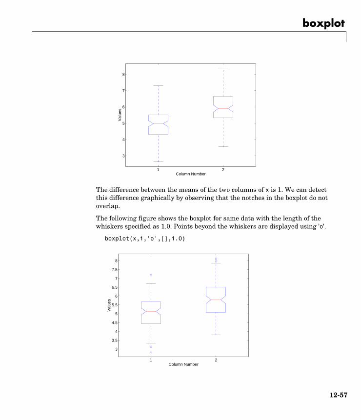
boxplot
The difference between the means of the two columns of x is 1. We can detect this difference graphically by observing that the notches in the boxplot do not overlap.
The following figure shows the boxplot for same data with the length of the whiskers specified as 1.0. Points beyond the whiskers are displayed using 'o'.
boxplot(x,1,'o',[],1.0)
1 2
3
4
5
6
7
8
Val
ues
Column Number
1 2
3
3.5
4
4.5
5
5.5
6
6.5
7
7.5
8
Val
ues
Column Number
12-57

boxplot
See Also anova1, kruskalwallis
12-58

candexch
12candexchPurpose D-optimal design from candidate set using row exchanges
Syntax rlist = candexch(C,nrows)rlist = candexch(C,nrows,'param1',value1,'param2',value2,...)
Description rlist = candexch(C,nrows) uses a row-exchange algorithm to select a D-optimal design from the candidate set C. C is an n-by-p matrix containing the values of p model terms at each of n points. nrows is the desired number of rows in the design. rlist is a vector of length nrows listing the selected rows.
The candexch function selects a starting design X at random, and uses a row-exchange algorithm to iteratively replace rows of X by rows of C in an attempt to improve the determinant of X'*X.
rlist = candexch(C,nrows,'param1',value1,'param2',value2,...)provides more control over the design generation through a set of parameter/value pairs. Valid parameters are the following:
Note The rowexch function also generates D-optimal designs using a row-exchange algorithm, but it accepts a model type and automatically selects a candidate set that is appropriate for such a model.
Examples Generate a D-optimal design when there is a restriction on the candidate set. In this case, the rowexch function isn't appropriate.
F = (fullfact([5 5 5])-1)/4; % Factor settings in unit cube.T = sum(F,2)<=1.51; % Find rows matching a restriction.
Parameter Value
'display' Either 'on' or 'off' to control display of iteration number The default is 'on'.
'init' Initial design as an nrows-by-p matrix. The default is a random subset of the rows of C.
'maxiter' Maximum number of iterations. The default is 10.
12-59

candexch
F = F(T,:); % Take only those rows.C = [ones(size(F,1),1) F F.^2]; % Compute model terms including % a constant and all squared terms.R = candexch(C,12); % Find a D-optimal 12-point subset.X = F(R,:); % Get factor settings.
See Also candgen, cordexch, rowexch, x2fx
12-60

candgen
12candgenPurpose Generate candidate set for D-optimal design
Syntax xcand = candgen(nfactors,'model')[xcand,fxcand] = candgen(nfactors,'model')
Description xcand = candgen(nfactors,'model') generates a candidate set appropriate for a D-optimal design with nfactors factors and the model model. The output matrix xcand has nfactors columns, with each row representing the coordinates of a candidate point. model is one of:
Alternatively, model can be a matrix of term definitions as accepted by the x2fx function.
[xcand,fxcand] = candgen(nfactors,model) returns both the matrix of factor values xcand and the matrix of term values fxcand. You can input the latter to candexch to generate the D-optimal design.
Note The rowexch function automatically generates a candidate set using candgen, and creates a D-optimal design from that candidate set using candexch. Call these functions separately if you want to modify the default candidate set.
See Also candexch, rowexch, x2fx
'linear' Constant and linear terms (the default)
'interaction' Constant, linear, and cross product terms
'quadratic' Interactions plus squared terms
'purequadratic' Constant, linear, and squared terms
12-61

canoncorr
12canoncorrPurpose Canonical correlation analysis
Syntax [A,B] = canoncorr(X,Y)[A,B,r] = canoncorr(X,Y)[A,B,r,U,V] = canoncorr(X,Y)[A,B,r,U,V,stats] = canoncorr(X,Y)
Description [A,B] = canoncorr(X,Y) computes the sample canonical coefficients for the n-by-d1 and n-by-d2 data matrices X and Y. X and Y must have the same number of observations (rows) but can have different numbers of variables (columns). A and B are d1-by-d and d2-by-d matrices, where d = min(rank(X),rank(Y)). The jth columns of A and B contain the canonical coefficients, i.e., the linear combination of variables making up the jth canonical variable for X and Y, respectively. Columns of A and B are scaled to make the covariances of the canonical variables, or scores, the identity matrix (see U and V below). If X or Y is less than full rank, canoncorr gives a warning and returns zeros in the rows of A or B corresponding to dependent columns of X or Y.
[A,B,r] = canoncorr(X,Y) also returns a 1-by-d vector containing the sample canonical correlations. The jth element of r is the correlation between the jth columns of U and V (see below).
[A,B,r,U,V] = canoncorr(X,Y) also returns the canonical variables, known also as scores. U and V are n-by-d matrices computed as
U = (X - repmat(mean(X),N,1))*AV = (Y - repmat(mean(Y),N,1))*B
[A,B,r,U,V,stats] = canoncorr(X,Y) also returns a structure containing information relating to the sequence of d null hypotheses , that the (k+1)st through dth correlations are all zero, for k = 0:(d-1). stats contains three fields, each a 1-by-d vector with elements corresponding to the values of k:
dfe Error degrees of freedom, i.e., (d1-k)*(d2-k)
chisq Bartlett's approximate chi-squared statistic for
p Right-tail significance level for
H0k( )
H0k( )
H0k( )
12-62

canoncorr
Examples load carbig;X = [Displacement Horsepower Weight Acceleration MPG];nans = sum(isnan(X),2) > 0;[A B r U V] = canoncorr(X(~nans,1:3), X(~nans,4:5));
plot(U(:,1),V(:,1),'.');xlabel('0.0025*Disp + 0.020*HP - 0.000025*Wgt');ylabel('-0.17*Accel + -0.092*MPG')
See Also manova1, princomp
References [1] Krzanowski, W.J., Principles of Multivariate Analysis, Oxford University Press, Oxford, 1988.
[2] Seber, G.A.F., Multivariate Observations, Wiley, New York, 1984.
−2 −1 0 1 2 3 4−4
−3
−2
−1
0
1
2
3
0.0025*Disp + 0.020*HP − 0.000025*Wgt
−0.
17*A
ccel
+ −
0.09
2*M
PG
12-63

capable
12capablePurpose Process capability indices
Syntax p = capable(data,specs)[p,Cp,Cpk] = capable(data,specs)
Description p = capable(data,specs) computes the probability that a sample, data, from some process falls outside the bounds specified in specs, a 2-element vector of the form [lower upper].
The assumptions are that the measured values in the vector data are normally distributed with constant mean and variance and that the measurements are statistically independent.
[p,Cp,Cpk] = capable(data,specs) additionally returns the capability indices Cp and Cpk.
Cp is the ratio of the range of the specifications to six times the estimate of the process standard deviation:
For a process that has its average value on target, a Cp of 1 translates to a little more than one defect per thousand. Recently, many industries have set a quality goal of one part per million. This would correspond to Cp = 1.6. The higher the value of Cp, the more capable the process.
Cpk is the ratio of difference between the process mean and the closer specification limit to three times the estimate of the process standard deviation:
where the process mean is µ. For processes that do not maintain their average on target, Cpk is a more descriptive index of process capability.
Example Imagine a machined part with specifications requiring a dimension to be within three thousandths of an inch of nominal. Suppose that the machining process cuts too thick by one thousandth of an inch on average and also has a
CpUSL LSL–
6σ--------------------------------=
Cpk min USL µ–3σ
----------------------- µ LSL–3σ
----------------------, =
12-64

capable
standard deviation of one thousandth of an inch. What are the capability indices of this process?
data = normrnd(1,1,30,1);[p,Cp,Cpk] = capable(data,[-3 3]);
indices = [p Cp Cpk]indices =
0.0172 1.1144 0.7053
We expect 17 parts out of a thousand to be out-of-specification. Cpk is less than Cp because the process is not centered.
Reference [1] Montgomery, D., “Introduction to Statistical Quality Control,” John Wiley & Sons 1991. pp. 369–374.
See Also capaplot, histfit
12-65

capaplot
12capaplotPurpose Process capability plot
Syntax p = capaplot(data,specs)[p,h] = capaplot(data,specs)
Description p = capaplot(data,specs) estimates the mean and variance of the observations in input vector data, and plots the pdf of the resulting T distribution. The observations in data are assumed to be normally distributed. The output, p, is the probability that a new observation from the estimated distribution will fall within the range specified by the two-element vector specs. The portion of the distribution between the lower and upper bounds specified in specs is shaded in the plot.
[p,h] = capaplot(data,specs) additionally returns handles to the plot elements in h.
Example Imagine a machined part with specifications requiring a dimension to be within 3 thousandths of an inch of nominal. Suppose that the machining process cuts too thick by one thousandth of an inch on average and also has a standard deviation of one thousandth of an inch.
data = normrnd(1,1,30,1);p = capaplot(data,[-3 3])p =
0.9784
The probability of a new observation being within specs is 97.84%.
-3 -2 -1 0 1 2 3 40
0.1
0.2
0.3
0.4Probability Between Limits is 0.9784
12-66

capaplot
See Also capable, histfit
12-67

caseread
12casereadPurpose Read casenames from a file
Syntax names = caseread('filename')names = caseread
Description names = caseread('filename') reads the contents of filename and returns a string matrix of names. filename is the name of a file in the current directory, or the complete pathname of any file elsewhere. caseread treats each line as a separate case.
names = caseread displays the Select File to Open dialog box for interactive selection of the input file.
Example Read the file months.dat created using the function casewrite on the next page.
type months.dat
JanuaryFebruaryMarchAprilMay
names = caseread('months.dat')names =
January FebruaryMarch April May
See Also tblread, gname, casewrite, tdfread
12-68

casewrite
12casewritePurpose Write casenames from a string matrix to a file
Syntax casewrite(strmat,'filename')casewrite(strmat)
Description casewrite(strmat,'filename') writes the contents of string matrix strmat to filename. Each row of strmat represents one casename. filename is the name of a file in the current directory, or the complete pathname of any file elsewhere. casewrite writes each name to a separate line in filename.
casewrite(strmat) displays the Select File to Write dialog box for interactive specification of the output file.
Example strmat = str2mat('January','February','March','April','May')
strmat =
January FebruaryMarch April May
casewrite(strmat,'months.dat')type months.dat
January FebruaryMarch April May
See Also gname, caseread, tblwrite, tdfread
12-69

ccdesign
12ccdesignPurpose Generate central composite design
Syntax D = ccdesign(nfactors)D = ccdesign(nfactors,'pname1',pvalue1,'pname2',pvalue2,...)[D,blk] = ccdesign(...)
Description D = ccdesign(nfactors) generates a central composite design for nfactors factors. The output matrix D is n-by-nfactors, where n is the number of points in the design. Each row represents one run of the design, and it has the settings of all factors for that run. Factor values are normalized so that the cube points take values between -1 and 1.
[D,blk] = ccdesign(nfactors) requests a blocked design. The output vector blk is a vector of block numbers. Blocks are groups of runs that are to be measured under similar conditions (for example, on the same day). Blocked designs minimize the effect of between-block differences on the parameter estimates.
[...] = ccdesign(nfactors,'pname1',pvalue1,'pname2',pvalue2,...)enables you to specify additional parameters and their values. Valid parameters are:
'center' Number of center points:
Integer Specific number of center points to include
'uniform' Number of center points is selected to give uniform precision
'orthogonal' Number of center points is selected to give an orthogonal design (default)
'fraction' Fraction of full factorial for cube portion expressed as an exponent of 1/2. For example:
0 Whole design
1 1/2 fraction
2 1/4 fraction
'type' Either 'inscribed', 'circumscribed', or 'faced'
'blocksize' Maximum number of points allowed in a block.
12-70

ccdesign
See Also bbdesign, cordexch, rowexch
12-71

cdf
12cdfPurpose Computes a chosen cumulative distribution function (cdf)
Syntax P = cdf('name',X,A1,A2,A3)
Description P = cdf('name',X,A1,A2,A3) returns a matrix of probabilities, where name is a string containing the name of the distribution, X is a matrix of values, and A, A2, and A3 are matrices of distribution parameters. Depending on the distribution, some of these parameters may not be necessary.
Vector or matrix inputs for X, A1, A2, and A3 must have the same size, which is also the size of P. A scalar input for X, A1, A2, or A3 is expanded to a constant matrix with the same dimensions as the other inputs.
cdf is a utility routine allowing you to access all the cdfs in the Statistics Toolbox by using the name of the distribution as a parameter. See “Overview of the Distributions” on page 2-11 for the list of available distributions.
Examples p = cdf('Normal',-2:2,0,1)p =
0.0228 0.1587 0.5000 0.8413 0.9772
p = cdf('Poisson',0:5,1:6)p =
0.3679 0.4060 0.4232 0.4335 0.4405 0.4457
See Also betacdf, binocdf, chi2cdf, expcdf, fcdf, gamcdf, geocdf, hygecdf, icdf, logncdf, mle, nbincdf, ncfcdf, nctcdf, ncx2cdf, normcdf, pdf, poisscdf, random, raylcdf, tcdf, unidcdf, unifcdf, weibcdf
12-72

cdfplot
12cdfplotPurpose Plot of empirical cumulative distribution function
Syntax cdfplot(X)h = cdfplot(X)[h,stats] = cdfplot(X)
Description cdfplot(X) displays a plot of the empirical cumulative distribution function (cdf) for the data in the vector X. The empirical cdf is defined as the proportion of X values less than or equal to x.
This plot, like those produced by hist and normplot, is useful for examining the distribution of a sample of data. You can overlay a theoretical cdf on the same plot to compare the empirical distribution of the sample to the theoretical distribution.
The kstest, kstest2, and lillietest functions compute test statistics that are derived from the empirical cdf. You may find the empirical cdf plot produced by cdfplot useful in helping you to understand the output from those functions.
H = cdfplot(X) returns a handle to the cdf curve.
[h,stats] = cdfplot(X) also returns a stats structure with the following fields.
Examples Generate a normal sample and an empirical cdf plot of the data.
x = normrnd(0,1,50,1);cdfplot(x)
Field Contents
stats.min Minimum value
stats.max Maximum value
stats.mean Sample mean
stats.median Sample median (50th percentile)
stats.std Sample standard deviation
F x( )
12-73

cdfplot
See Also ecdf, hist, kstest, kstest2, lillietest, normplot
−3 −2 −1 0 1 2 30
0.1
0.2
0.3
0.4
0.5
0.6
0.7
0.8
0.9
1
x
F(x
)
Empirical CDF
12-74

chi2cdf
12chi2cdfPurpose Chi-square (χ2) cumulative distribution function (cdf)
Syntax P = chi2cdf(X,V)
Description P = chi2cdf(X,V) computes the χ2 cdf at each of the values in X using the corresponding parameters in V. Vector or matrix inputs for X and V must have the same size. A scalar input is expanded to a constant matrix with the same dimensions as the other input. The degrees of freedom parameters in V must be positive integers, and the values in X must lie on the interval [0 1].
The χ2 cdf for a given value x and degrees-of-freedom ν is
where Γ( · ) is the Gamma function. The result, p, is the probability that a single observation from a χ2 distribution with ν degrees of freedom will fall in the interval [0 x].
The χ2 density function with ν degrees-of-freedom is the same as the gamma density function with parameters ν/2 and 2.
Examples probability = chi2cdf(5,1:5)probability =
0.9747 0.9179 0.8282 0.7127 0.5841
probability = chi2cdf(1:5,1:5)probability =
0.6827 0.6321 0.6084 0.5940 0.5841
See Also cdf, chi2inv, chi2pdf, chi2rnd, chi2stat
p F x ν( ) t ν 2–( ) 2⁄ e t– 2⁄
2ν 2⁄ Γ ν 2⁄( )-----------------------------------
0
x
∫ dt= =
12-75

chi2inv
12chi2invPurpose Inverse of the chi-square (χ2) cumulative distribution function (cdf)
Syntax X = chi2inv(P,V)
Description X = chi2inv(P,V) computes the inverse of the χ2 cdf with parameters specified by V for the corresponding probabilities in P. Vector or matrix inputs for P and V must have the same size. A scalar input is expanded to a constant matrix with the same dimensions as the other inputs.
The degrees of freedom parameters in V must be positive integers, and the values in P must lie in the interval [0 1].
The inverse χ2 cdf for a given probability p and ν degrees of freedom is
where
and Γ( · ) is the Gamma function. Each element of output X is the value whose cumulative probability under the χ2 cdf defined by the corresponding degrees of freedom parameter in V is specified by the corresponding value in P.
Examples Find a value that exceeds 95% of the samples from a χ2 distribution with 10 degrees of freedom.
x = chi2inv(0.95,10)x =
18.3070
You would observe values greater than 18.3 only 5% of the time by chance.
See Also chi2cdf, chi2pdf, chi2rnd, chi2stat, icdf
x F 1– p ν( ) x:F x ν( ) p={ }= =
p F x ν( ) t ν 2–( ) 2⁄ e t– 2⁄
2ν 2⁄ Γ ν 2⁄( )-----------------------------------
0
x
∫ dt= =
12-76
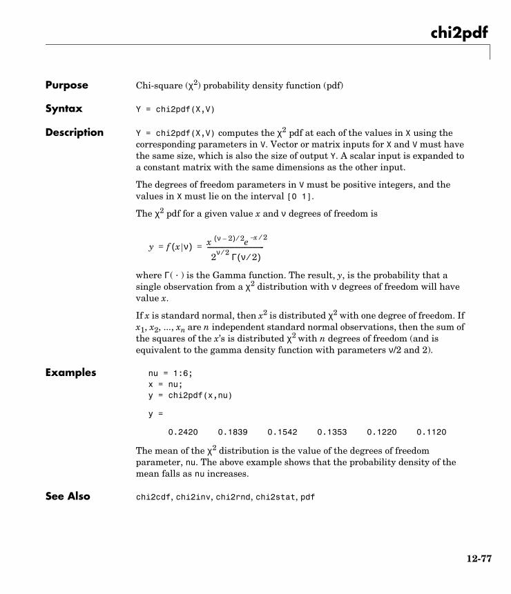
chi2pdf
12chi2pdfPurpose Chi-square (χ2) probability density function (pdf)
Syntax Y = chi2pdf(X,V)
Description Y = chi2pdf(X,V) computes the χ2 pdf at each of the values in X using the corresponding parameters in V. Vector or matrix inputs for X and V must have the same size, which is also the size of output Y. A scalar input is expanded to a constant matrix with the same dimensions as the other input.
The degrees of freedom parameters in V must be positive integers, and the values in X must lie on the interval [0 1].
The χ2 pdf for a given value x and ν degrees of freedom is
where Γ( · ) is the Gamma function. The result, y, is the probability that a single observation from a χ2 distribution with ν degrees of freedom will have value x.
If x is standard normal, then x2 is distributed χ2 with one degree of freedom. If x1, x2, ..., xn are n independent standard normal observations, then the sum of the squares of the x’s is distributed χ2 with n degrees of freedom (and is equivalent to the gamma density function with parameters ν/2 and 2).
Examples nu = 1:6;x = nu;y = chi2pdf(x,nu)
y =
0.2420 0.1839 0.1542 0.1353 0.1220 0.1120
The mean of the χ2 distribution is the value of the degrees of freedom parameter, nu. The above example shows that the probability density of the mean falls as nu increases.
See Also chi2cdf, chi2inv, chi2rnd, chi2stat, pdf
y f x ν( ) x ν 2–( ) 2⁄ e x– 2⁄
2ν 2⁄ Γ ν 2⁄( )-------------------------------------= =
12-77

chi2rnd
12chi2rndPurpose Random numbers from the chi-square (χ2) distribution
Syntax R = chi2rnd(V)R = chi2rnd(V,m)R = chi2rnd(V,m,n)
Description R = chi2rnd(V) generates random numbers from the χ2 distribution with degrees of freedom parameters specified by V. R is the same size as V.
R = chi2rnd(V,m) generates a matrix of size m containing random numbers from the χ2 distribution with degrees of freedom parameter V, where m is a 1-by-2 vector containing the row and column dimensions of R.
R = chi2rnd(V,m,n) generates an m-by-n matrix containing random numbers from the χ2 distribution with degrees of freedom parameter V.
Examples Note that the first and third commands are the same, but are different from the second command.
r = chi2rnd(1:6)r =
0.0037 3.0377 7.8142 0.9021 3.2019 9.0729
r = chi2rnd(6,[1 6])r =
6.5249 2.6226 12.2497 3.0388 6.3133 5.0388
r = chi2rnd(1:6,1,6)r =
0.7638 6.0955 0.8273 3.2506 1.5469 10.9197
See Also chi2cdf, chi2inv, chi2pdf, chi2stat
12-78
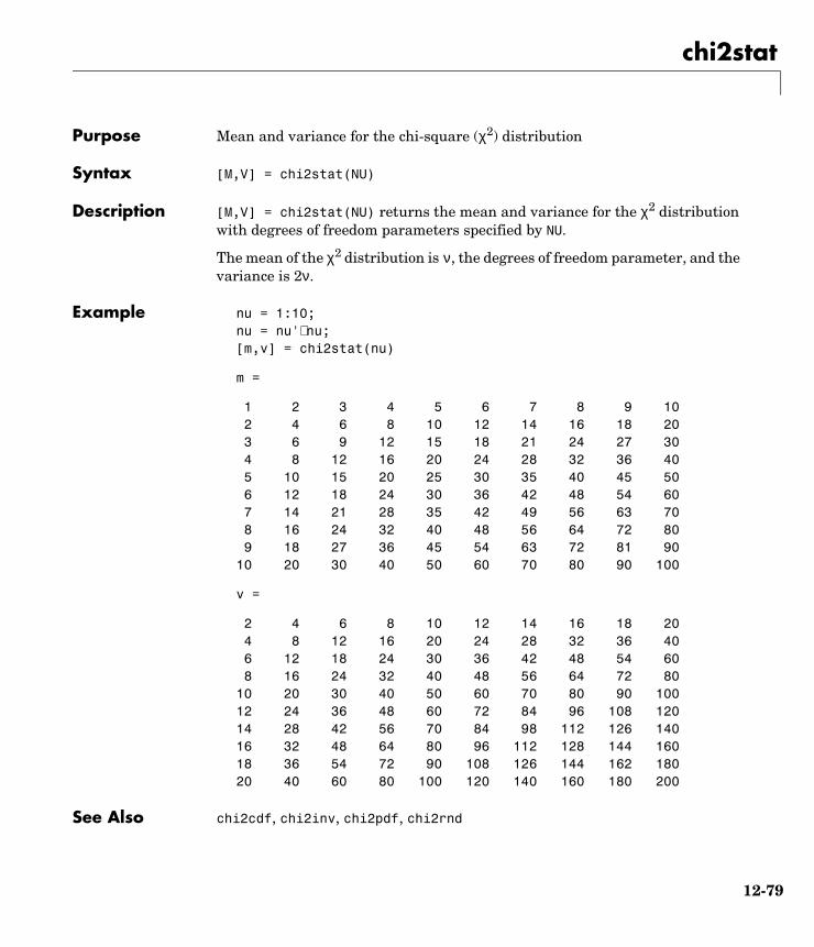
chi2stat
12chi2statPurpose Mean and variance for the chi-square (χ2) distribution
Syntax [M,V] = chi2stat(NU)
Description [M,V] = chi2stat(NU) returns the mean and variance for the χ2 distribution with degrees of freedom parameters specified by NU.
The mean of the χ2 distribution is ν, the degrees of freedom parameter, and the variance is 2ν.
Example nu = 1:10;nu = nu'∗ nu;[m,v] = chi2stat(nu)
m =
1 2 3 4 5 6 7 8 9 10 2 4 6 8 10 12 14 16 18 20 3 6 9 12 15 18 21 24 27 30 4 8 12 16 20 24 28 32 36 40 5 10 15 20 25 30 35 40 45 50 6 12 18 24 30 36 42 48 54 60 7 14 21 28 35 42 49 56 63 70 8 16 24 32 40 48 56 64 72 80 9 18 27 36 45 54 63 72 81 9010 20 30 40 50 60 70 80 90 100
v =
2 4 6 8 10 12 14 16 18 20 4 8 12 16 20 24 28 32 36 40 6 12 18 24 30 36 42 48 54 60 8 16 24 32 40 48 56 64 72 8010 20 30 40 50 60 70 80 90 10012 24 36 48 60 72 84 96 108 12014 28 42 56 70 84 98 112 126 14016 32 48 64 80 96 112 128 144 16018 36 54 72 90 108 126 144 162 18020 40 60 80 100 120 140 160 180 200
See Also chi2cdf, chi2inv, chi2pdf, chi2rnd
12-79

classify
12classifyPurpose Discriminant Analysis
Syntax class = classify(sample,training,group)[class,err] = classify(...)[...] = classify(...,'type')[...] = classify(...,'type',prior)
Description class = classify(sample,training,group) classifies each row of the data in sample into one of the groups in training. sample and training must be matrices with the same number of columns. group is a grouping variable for training. Its unique values define groups, and each element defines which group the corresponding row of training belongs to. group can be a numeric vector, a string array, or a cell array of strings. training and group must have the same number of rows. classify treats NaNs or empty strings in group as missing values, and ignores the corresponding rows of training. class indicates which group each row of sample has been assigned to, and is of the same type as group.
[class,err] = classify(...) also returns an estimate of the misclassification error rate. classify returns the apparent error rate, i.e., the percentage of observations in the training that are misclassified.
[...] = classify(...,'type') allows you to specify the type of discriminant function, as one of:
[...] = classify(...,'type',prior) enables you to specify prior probabilities for the groups in one of three ways. prior can be:
• A numeric vector of the same length as the number of unique values in group. If group is numeric, the order of prior must correspond to the sorted
'linear' Fits a multivariate normal density to each group, with a pooled estimate of covariance (default).
'quadratic' Fits MVN densities with covariance estimates stratified by group.
'mahalanobis' Uses Mahalanobis distances with stratified covariance estimates.
12-80

classify
values in group, or, if group contains strings, to the order of first occurrence of the values in group.
• A 1-by-1 structure with fields:
As a structure, prior can contain groups that do not appear in group. This can be useful if training is a subset a larger training set.
• The string value 'empirical', indicating that classify should estimate the group prior probabilities from the group relative frequencies in training.
prior defaults to a numeric vector of equal probabilities, i.e., a uniform distribution. prior is not used for discrimination by Mahalanobis distance, except for error rate calculation.
Examples load discrimsample = ratings(idx,:);training = ratings(1:200,:);g = group(1:200);class = classify(sample,training,g);first5 = class(1:5)
first5 =
2 2 2 2 2
See Also mahal
References [1] Krzanowski, W.J., Principles of Multivariate Analysis, Oxford University Press, Oxford, 1988.
[2] Seber, G.A.F., Multivariate Observations, Wiley, New York, 1984
prob A numeric vector
group Of the same type as group, and containing unique values indicating which groups the elements of prob correspond to.
12-81
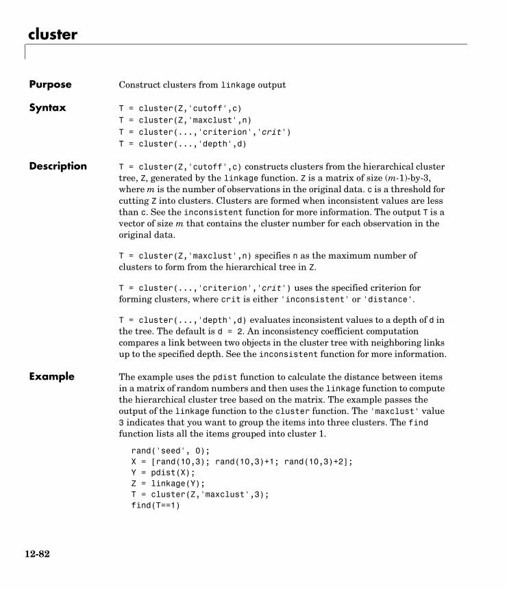
cluster
12clusterPurpose Construct clusters from linkage output
Syntax T = cluster(Z,'cutoff',c)T = cluster(Z,'maxclust',n)T = cluster(...,'criterion','crit')T = cluster(...,'depth',d)
Description T = cluster(Z,'cutoff',c) constructs clusters from the hierarchical cluster tree, Z, generated by the linkage function. Z is a matrix of size (m-1)-by-3, where m is the number of observations in the original data. c is a threshold for cutting Z into clusters. Clusters are formed when inconsistent values are less than c. See the inconsistent function for more information. The output T is a vector of size m that contains the cluster number for each observation in the original data.
T = cluster(Z,'maxclust',n) specifies n as the maximum number of clusters to form from the hierarchical tree in Z.
T = cluster(...,'criterion','crit') uses the specified criterion for forming clusters, where crit is either 'inconsistent' or 'distance'.
T = cluster(...,'depth',d) evaluates inconsistent values to a depth of d in the tree. The default is d = 2. An inconsistency coefficient computation compares a link between two objects in the cluster tree with neighboring links up to the specified depth. See the inconsistent function for more information.
Example The example uses the pdist function to calculate the distance between items in a matrix of random numbers and then uses the linkage function to compute the hierarchical cluster tree based on the matrix. The example passes the output of the linkage function to the cluster function. The 'maxclust' value 3 indicates that you want to group the items into three clusters. The find function lists all the items grouped into cluster 1.
rand('seed', 0); X = [rand(10,3); rand(10,3)+1; rand(10,3)+2]; Y = pdist(X); Z = linkage(Y); T = cluster(Z,'maxclust',3); find(T==1)
12-82

cluster
ans = 11121314151617181920
See Also clusterdata, cophenet, inconsistent, linkage, pdist
12-83

clusterdata
12clusterdataPurpose Construct clusters from data
Syntax T = clusterdata(X, cutoff)T = clusterdata(X,'param1',val1,'param2',val2,...)
Description T = clusterdata(X, cutoff) uses the pdist, linkage, and cluster functions to construct clusters from data X. X is an m-by-n matrix, treated as m observations of n variables. cutoff is a threshold for cutting the hierarchical tree generated by linkage into clusters. When 0 < cutoff < 2, clusterdata forms clusters when inconsistent values are greater than cutoff (see the inconsistent function). When cutoff is an integer and cutoff >= 2, then clusterdata inteprets cutoff as the maximum number of clusters to keep in the hierarchical tree generated by linkage. The output T is a vector of size m containing a cluster number for each observation.
T = clusterdata(X,cutoff) is the same as
Y = pdist(X,'euclid'); Z = linkage(Y,'single'); T = cluster(Z,'cutoff',cutoff);
T = clusterdata(X,'param1',val1,'param2',val2,...) provides more control over the clustering through a set of parameter/value pairs. Valid parameters are:
Example The example first creates a sample dataset of random numbers. It then uses clusterdata to compute the distances between items in the dataset and create a hierarchical cluster tree from the dataset. Finally, the clusterdata function
'distance' Any of the distance metric names allowed by pdist (follow the 'minkowski' option by the value of the exponent p).
'linkage' Any of the linkage methods allowed by the linkage function
'cutoff' Cutoff for inconsistent or distance measure
'maxclust' Maximum number of clusters to form
'criterion' Either 'inconsistent' or 'distance'
'depth' Depth for computing inconsistent values
12-84

clusterdata
groups the items in the dataset into three clusters. The example uses the find function to list all the items in cluster 2.
rand('seed',12); X = [rand(10,3); rand(10,3)+1.2; rand(10,3)+2.5]; T = clusterdata(X,'maxclust',3); find(T==2)
ans = 21 22 23 24 25 26 27 28 29 30
See Also cluster, inconsistent, kmeans, linkage, pdist
12-85

cmdscale
12cmdscalePurpose Classical multidimensional scaling
Syntax Y = cmdscale(D)[Y,e] = cmdscale(D)
Description Y = cmdscale(D) takes an n-by-n distance matrix D, and returns an n-by-p configuration matrix Y. Rows of Y are the coordinates of n points in p-dimensional space for some p < n. When D is a Euclidean distance matrix, the distances between those points are given by D. p is the dimension of the smallest space in which the n points whose interpoint distances are given by D can be embedded.
[Y,e] = cmdscale(D) also returns the eigenvalues of Y*Y'. When D is Euclidean, the first p elements of e are positive, the rest zero. If the first k elements of e are much larger than the remaining (n-k), then you can use the first k columns of Y as k-dimensional points whose interpoint distances approximate D. This can provide a useful dimension reduction for visualization, e.g., for k = 2.
D need not be a Euclidean distance matrix. If it is non-Euclidean or a more general dissimilarity matrix, then some elements of e are negative, and cmdscale choses p as the number of positive eigenvalues. In this case, the reduction to p or fewer dimensions provides a reasonable approximation to D only if the negative elements of e are small in magnitude.
You can specify D as either a full dissimilarity matrix, or in upper triangle vector form such as is output by pdist. A full dissimilarity matrix must be real and symmetric, and have zeros along the diagonal and positive elements everywhere else. A dissimilarity matrix in upper triangle form must have real, positive entries. You can also specify D as a full similarity matrix, with ones along the diagonal and all other elements less than one. cmdscale tranforms a similarity matrix to a dissimilarity matrix in such a way that distances between the points returned in Y equal or approximate sqrt(1-D). To use a different transformation, you must transform the similarities prior to calling cmdscale.
Examples Generate some points in 4-dimensional space, but "close" to 3-dimensional space, then reduce them to distances only.
12-86

cmdscale
X = [normrnd(0,1,10,3) normrnd(0,.1,10,1)];D = pdist(X,'euclidean');
Find a configuration with those inter-point distances.
[Y,e] = cmdscale(D);% Four, but fourth one smalldim = sum(e > eps^(3/4))% Poor reconstructionmaxerr2 = max(abs(pdist(X) - pdist(Y(:,1:2)))) % Good reconstructionmaxerr3 = max(abs(pdist(X) - pdist(Y(:,1:3)))) % Exact reconstructionmaxerr4 = max(abs(pdist(X) - pdist(Y)))% D is now non-EuclideanD = pdist(X,'cityblock');[Y,e] = cmdscale(D);% One is large negativemin(e)% Poor reconstructionmaxerr = max(abs(pdist(X) - pdist(Y)))
See Also pdist, procrustes
References [1] Seber, G.A.F., Multivariate Observations, Wiley, 1984
12-87

combnk
12combnkPurpose Enumeration of all combinations of n objects k at a time
Syntax C = combnk(v,k)
Description C = combnk(v,k) returns all combinations of the n elements in v taken k at a time.
C = combnk(v,k) produces a matrix C with k columns and n! / k!(n-k)! rows, where each row contains k of the elements in the vector v.
It is not practical to use this function if v has more than about 15 elements.
Example Combinations of characters from a string.
C = combnk('tendril',4);last5 = C(31:35,:)
last5 =
tedrtenltenitenrtend
Combinations of elements from a numeric vector.
c = combnk(1:4,2)
c = 3 4 2 4 2 3 1 4 1 3 1 2
12-88

cophenet
12cophenetPurpose Cophenetic correlation coefficient
Syntax c = cophenet(Z,Y)
Description c = cophenet(Z,Y) computes the cophenetic correlation coefficient which compares the distance information in Z, generated by linkage, and the distance information in Y, generated by pdist. Z is a matrix of size (m-1)-by-3, with distance information in the third column. Y is a vector of size
.
For example, given a group of objects {1, 2, ..., m} with distances Y, the function linkage produces a hierarchical cluster tree. The cophenet function measures the distortion of this classification, indicating how readily the data fits into the structure suggested by the classification.
The output value, c, is the cophenetic correlation coefficient. The magnitude of this value should be very close to 1 for a high-quality solution. This measure can be used to compare alternative cluster solutions obtained using different algorithms.
The cophenetic correlation between Z(:,3) and Y is defined as
where:
• Yij is the distance between objects i and j in Y.
• Zij is the distance between objects i and j in Z(:,3).
• y and z are the average of Y and Z(:,3), respectively.
Example rand('seed',12); X = [rand(10,3);rand(10,3)+1;rand(10,3)+2];Y = pdist(X);Z = linkage(Y,'centroid');c = cophenet(Z,Y)
c = 0.6985
m m 1–( ) 2⁄⋅
cΣi j< Yij y–( ) Zij z–( )
Σi j< Yij y–( )2Σi j< Zij z–( )2------------------------------------------------------------------------------=
12-89

cophenet
See Also cluster, dendrogram, inconsistent, linkage, pdist, squareform
12-90

cordexch
12cordexchPurpose D-optimal design of experiments – coordinate exchange algorithm
Syntax settings = cordexch(nfactors,nruns)[settings,X] = cordexch(nfactors,nruns)[settings,X] = cordexch(nfactors,nruns,'model')[settings,X] = cordexch(...,'param1',value1,'param2',value2,...)
Description settings = cordexch(nfactors,nruns) generates the factor settings matrix, settings, for a D-optimal design using a linear additive model with a constant term. settings has nruns rows and nfactors columns.
[settings,X] = cordexch(nfactors,nruns) also generates the associated design matrix X.
[settings,X] = cordexch(nfactors,nruns,'model') produces a design for fitting a specified regression model. The input, 'model', can be one of these strings:
Alternatively model can be a matrix of term definitions as accepted by the x2fx function.
[settings,X] = cordexch(...,'param1',value1,'param2',value2,...)provides more control over the design generation through a set of parameter/value pairs. Valid parameters are:
'linear' Includes constant and linear terms (the default)
'interaction' Includes constant, linear, and cross-product terms.
'quadratic' Includes interactions and squared terms.
'purequadratic' Includes constant, linear and squared terms.
'display' Either 'on' or 'off' to control display of iteration counter. The default is 'on'.
'init' Initial design as an nruns-by-nfactors matrix. The default is a randomly selected set of points.
'maxiter' Maximum number of iterations. The default is 10.
12-91
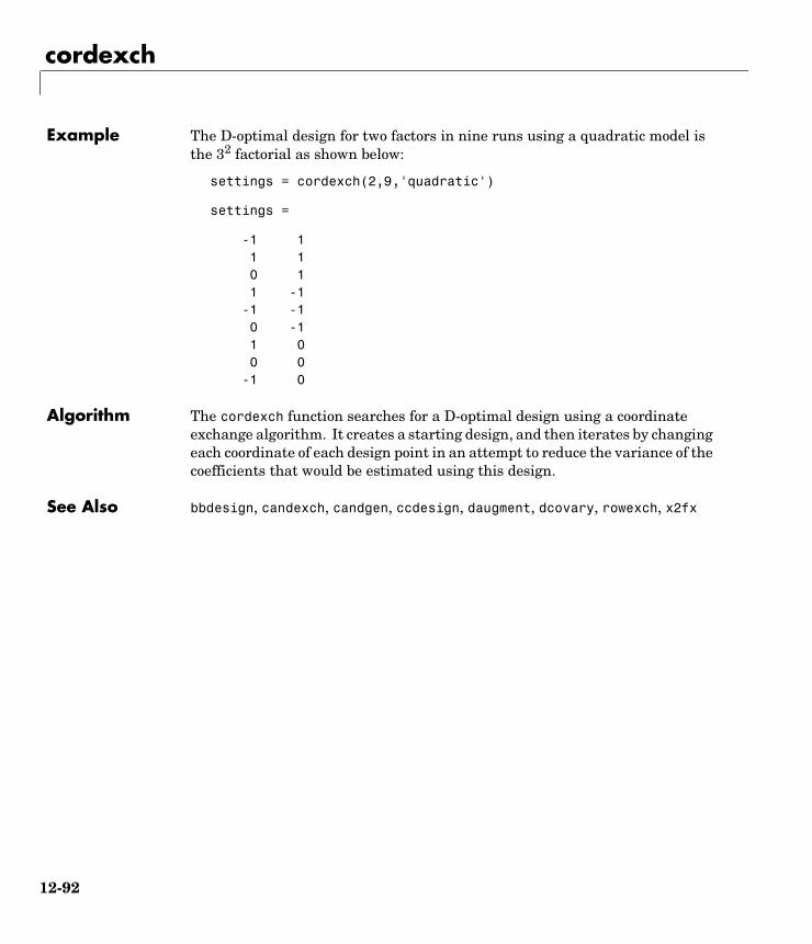
cordexch
Example The D-optimal design for two factors in nine runs using a quadratic model is the 32 factorial as shown below:
settings = cordexch(2,9,'quadratic')
settings =
-1 1 1 1 0 1 1 -1 -1 -1 0 -1 1 0 0 0 -1 0
Algorithm The cordexch function searches for a D-optimal design using a coordinate exchange algorithm. It creates a starting design, and then iterates by changing each coordinate of each design point in an attempt to reduce the variance of the coefficients that would be estimated using this design.
See Also bbdesign, candexch, candgen, ccdesign, daugment, dcovary, rowexch, x2fx
12-92

corr
12corrPurpose Correlation coefficients with tests and confidence bounds
Syntax R = corr(X)R = corr(x,y)[R,P] = corr(...)[R,P,RLO,RUP] = corr(...)[...] = corr(...,'param1',val1,'param2',val2,...)
Description R = corr(X) calculates a matrix R of correlation coefficients for an array X Each row of X is an observation and each column is a variable. NaN (not a number) values in X are treated as missing.
If C is the covariance matrix, C = cov(X), then corr(X) is the matrix whose (i,j)th element is
R = corr(x,y) where x and y are column vectors, is the same as R = corr([x y]).
[R,P] = corr(...) also returns P, a matrix of p-values for testing the hypothesis of no correlation. Each p-value is the probability of getting a correlation as large as the observed value by random chance, when the true correlation is zero. If P(i,j) is small, say less than 0.05, then the correlation R(i,j) is significant. See “Algorithm” for details.
[R,P,RLO,RUP] = corr(...) also returns matrices RLO and RUP, of the same size as R, containing lower and upper bounds for a 95% confidence interval for each coefficient.
[...] = corr(...,'param1',val1,'param2',val2,...) specifies additional parameters and their values. Valid parameters are the following:
'alpha' A number between 0 and 1 that specifies a confidence level of 100*(1-alpha)%. Default is 0.05 for 95% confidence intervals.
C i j ),( )C i i,( )C j j,( )-------------------------------------
12-93

corr
Examples load hogg; % load sample data [r,p,rlo,rup] = corr([x1 x2 x3 x4 x5],'alpha',0.10); [i,j] = find(p<0.05); % find significant correlations [i,j] % display their indices
Algorithm The p-value is computed by transforming the correlation to create an F statistic having 1 and n-2 degrees of freedom, where n is the number of rows of X. The confidence bounds are based on an asymptotic normal distribution for 0.5*log((1+R)/(1-R)), with an approximate variance equal to 1/(n-3). These bounds are accurate for large samples when X has a multivariate normal distribution.
See Also corrcoef, cov, nanmean, nanstd, std
'rows' 'all' Use all rows.
'complete' Use rows with no missing values (default).
'pairwise' Compute R(i,j) using rows with no missing values in column i or j.
12-94

corrcoef
12corrcoefPurpose Correlation coefficients
Syntax R = corrcoef(X)R = corrcoef(x,y)[R,P]=corrcoef(...)[R,P,RLO,RUP]=corrcoef(...)[...]=corrcoef(...,'param1',val1,'param2',val2,...)
Description R = corrcoef(X) returns a matrix R of correlation coefficients calculated from an input matrix X whose rows are observations and whose columns are variables. The (i,j)th element of the matrix R is related to the covariance matrix C = cov(X) by
corrcoef(X) is the zeroth lag of the covariance function, that is, the zeroth lag of xcov(x,'coeff') packed into a square array.
R = corrcoef(x,y) where x and y are column vectors is the same as corrcoef([x y]).
[R,P]=corrcoef(...) also returns P, a matrix of p-values for testing the hypothesis of no correlation. Each p-value is the probability of getting a correlation as large as the observed value by random chance, when the true correlation is zero. If P(i,j) is small, say less than 0.05, then the correlation R(i,j) is significant.
[R,P,RLO,RUP]=corrcoef(...) also returns matrices RLO and RUP, of the same size as R, containing lower and upper bounds for a 95% confidence interval for each coefficient.
[...]=corrcoef(...,'param1',val1,'param2',val2,...) specifies additional parameters and their values. Valid parameters are the following.
R i j,( ) C i j,( )C i i,( )C j j,( )-------------------------------------=
12-95

corrcoef
The p-value is computed by transforming the correlation to create a t statistic having n-2 degrees of freedom, where n is the number of rows of X. The confidence bounds are based on an asymptotic normal distribution of 0.5*log((1+R)/(1-R)), with an approximate variance equal to 1/(n-3). These bounds are accurate for large samples when X has a multivariate normal distribution. The 'pairwise' option can produce an R matrix that is not positive definite.
The corrcoef function is part of the standard MATLAB language.
Examples Generate random data having correlation between column 4 and the other columns.
x = randn(30,4); % Uncorrelated datax(:,4) = sum(x,2); % Introduce correlation.[r,p] = corrcoef(x) % Compute sample correlation and p-values.[i,j] = find(p<0.05); % Find significant correlations.[i,j] % Display their (row,col) indices.
r = 1.0000 -0.3566 0.1929 0.3457 -0.3566 1.0000 -0.1429 0.4461 0.1929 -0.1429 1.0000 0.5183 0.3457 0.4461 0.5183 1.0000
p = 1.0000 0.0531 0.3072 0.0613 0.0531 1.0000 0.4511 0.0135 0.3072 0.4511 1.0000 0.0033 0.0613 0.0135 0.0033 1.0000
ans = 4 2
'alpha' A number between 0 and 1 to specify a confidence level of 100*(1 - alpha)%. Default is 0.05 for 95% confidence intervals.
'rows' Either 'all' (default) to use all rows, 'complete' to use rows with no NaN values, or 'pairwise' to compute R(i,j) using rows with no NaN values in either column i or j.
12-96

corrcoef
4 3 2 4 3 4
See Also cov, mean, std, var
xcorr, xcov in the Signal Processing Toolbox
12-97

cov
12covPurpose Covariance matrix.
Syntax C = cov(X)C = cov(x,y)
Description C = cov(X) computes the covariance matrix. For a single vector, cov(x) returns a scalar containing the variance. For matrices, where each row is an observation, and each column a variable, cov(X) is the covariance matrix.
The variance function, var(X) is the same as diag(cov(X)).
The standard deviation function, std(X) is equivalent to sqrt(diag(cov(X))).
cov(x,y), where x and y are column vectors of equal length, gives the same result as cov([x y]).
The cov function is part of the standard MATLAB language.
Algorithm The algorithm for cov is
[n,p] = size(X);X = X - ones(n,1) * mean(X);Y = X'∗ X/(n-1);
See Also corrcoef, mean, std, var
xcov, xcorr (Signal Processing Toolbox)
12-98

crosstab
12crosstabPurpose Cross-tabulation of several vectors
Syntax table = crosstab(col1,col2)table = crosstab(col1,col2,col3,...)[table,chi2,p] = crosstab(col1,col2)[table,chi2,p,label] = crosstab(col1,col2)
Description table = crosstab(col1,col2) takes two vectors of positive integers and returns a matrix, table, of cross-tabulations. The ijth element of table contains the count of all instances where col1 = i and col2 = j.
Alternatively, col1 and col2 can be vectors containing noninteger values, character arrays, or cell arrays of strings. crosstab implicitly assigns a positive integer group number to each distinct value in col1 and col2, and creates a cross-tabulation using those numbers.
table = crosstab(col1,col2,col3,...) returns table as an n-dimensional array, where n is the number of arguments you supply. The value of table(i,j,k,...) is the count of all instances where col1 = i, col2 = j, col3 = k, and so on.
[table,chi2,p] = crosstab(col1,col2) also returns the chi-square statistic, chi2, for testing the independence of the rows and columns of table. The scalar p is the significance level of the test. Values of p near zero cast doubt on the assumption of independence of the rows and columns of table.
[table,chi2,p,label] = crosstab(col1,col2) also returns a cell array label that has one column for each input argument. The value in label(i,j) is the value of colj that defines group i in the jth dimension.
Example Example 1We generate 2 columns of 50 discrete uniform random numbers. The first column has numbers from 1 to 3. The second has only the numbers 1 and 2. The two columns are independent so we would be surprised if p were near zero.
r1 = unidrnd(3,50,1);r2 = unidrnd(2,50,1);[table,chi2,p] = crosstab(r1,r2)
table =
12-99

crosstab
10 5 8 8 6 13
chi2 =
4.1723
p =
0.1242
The result, 0.1242, is not a surprise. A very small value of p would make us suspect the “randomness” of the random number generator.
Example 2We have data collected on several cars over a period of time. How many four-cylinder cars were made in the USA during the late part of this period?
[t,c,p,l] = crosstab(cyl4,when,org);
ll = 'Other' 'Early' 'USA' 'Four' 'Mid' 'Europe' [] 'Late' 'Japan'
t(2,3,1)
ans = 38
See Also tabulate
12-100

daugment
12daugmentPurpose D-optimal augmentation of an experimental design
Syntax settings = daugment(startdes,nruns)[settings,X] = daugment(startdes,nruns)[settings,X] = daugment(startdes,nruns,'model')[settings, X] = daugment(...,'param1',value1,'param2',value2,...)
Description settings = daugment(startdes,nruns) adds nruns runs to an experimental design using the coordinate exchange D-optimal algorithm. startdes is a matrix of factor settings in the original design. The output matrix settings is the matrix of factor settings for the design.
[settings,X] = daugment(startdes,nruns) also generates the associated design matrix, X.
[settings,X] = daugment(startdes,nruns,'model') also controls the order of the regression model. The input, 'model', can be one of these:
Alternatively model can be a matrix of term definitions as accepted by the x2fx function.
[settings, X] = daugment(...,'param1',value1,'param2',value2,...)provides more control over the design generation through a set of parameter/value pairs. Valid parameters are the following::
'linear' Includes constant and linear terms (the default)
'interaction' Includes constant, linear, and cross-product terms.
'quadratic' Includes interactions and squared terms.
'purequadratic' Includes constant, linear and squared terms.
Parameter Value
'display' Either 'on' or 'off' to control display of iteration counter. The default is 'on'.
12-101

daugment
Example We add 5 runs to a 22 factorial design to allow us to fit a quadratic model.
startdes = [-1 -1; 1 -1; -1 1; 1 1];settings = daugment(startdes,5,'quadratic')
settings =
-1 -1 1 -1 -1 1 1 1 1 0 -1 0 0 1 0 0 0 -1
The result is a 32 factorial design.
See Also cordexch, x2fx
'init' Initial design as an nruns-by-nfactors matrix. The default is a randomly selected set of points.
'maxiter' Maximum number of iterations. The default is 10.
Parameter Value
12-102

dcovary
12dcovaryPurpose D-optimal design with specified fixed covariates
Syntax settings = dcovary(nfactors,covariates)[settings,X] = dcovary(nfactors,covariates)[settings,X] = dcovary(nfactors,covariates,'model')[settings,X] = dcovary(...,'param1',value1,'param2',value2,...)
Description settings = dcovary(nfactors,covariates) uses a coordinate exchange algorithm to generate a D-optimal design for nfactors factors, subject to the constraint that it also include the fixed covariate values in the input matrix covariates. The number of runs in the design is taken to be the number of rows in the covariates matrix. The output matrix settings is the matrix of factor settings for the design, including the fixed covariates.
[settings,X] = dcovary(nfactors,covariates) also generates the associated design matrix, X.
[settings,X] = dcovary(nfactors,covariates,'model') also controls the order of the regression model. The input, 'model', can be one of these:
Alternatively 'model' can be a matrix of term definitions as accepted by the x2fx function. The model is applied to the fixed covariates as well as the regular factors. If you want to treat the fixed covariates specially, for example by including linear terms for them but quadratic terms for the regular factors, you can do this by creating the proper 'model' matrix.
[settings, X] = dcovary(...,'param1',value1,'param2',value2,...)provides more control over the design generation through a set of parameter/value pairs. Valid parameters are:
'linear' Includes constant and linear terms (the default)
'interaction' Includes constant, linear, and cross-product terms.
'quadratic' Includes interactions and squared terms.
'purequadratic' Includes constant, linear and squared terms.
12-103

dcovary
Example Example 1. Generate a design for three factors in 2 blocks of 4 runs.
blk = [-1 -1 -1 -1 1 1 1 1]';dsgn = dcovary(3,blk)
dsgn = -1 1 1 -1 1 -1 -1 -1 -1 1 -1 -1 1 -1 1 -1 1 1 -1 1 1 1 1 1 -1 -1 1 1 -1 -1 -1 1
Example 2. Suppose we want to block an eight run experiment into 4 blocks of size 2 to fit a linear model on two factors.
covariates = dummyvar([1 1 2 2 3 3 4 4]);settings = dcovary(2,covariates(:,1:3),'linear')settings = 1 1 1 0 0 -1 -1 1 0 0 -1 1 0 1 0 1 -1 0 1 0 1 1 0 0 1 -1 -1 0 0 1 -1 1 0 0 0 1 -1 0 0 0
The first two columns of the output matrix contain the settings for the two factors. The last three columns are dummy variable codings for the four blocks.
'display' Either 'on' or 'off' to control display of iteration counter. The default is 'on'.
'init' Initial design as an nruns-by-nfactors matrix. The default is a randomly selected set of points.
'maxiter' Maximum number of iterations. The default is 10.
12-104

dcovary
Algorithm The dcovary function creates a starting design that includes the fixed covariate values, and then iterates by changing the non-fixed cordinates of each design point in an attempt to reduce the variance of the coefficients that would be estimated using this design.
See Also cordexch, daugment, rowexch, x2fx
12-105

dendrogram
12dendrogramPurpose Plot dendrogram graphs
Syntax H = dendrogram(Z) H = dendrogram(Z,p)[H,T] = dendrogram(...)[H,T,perm] = dendrogram(...)[...] = dendrogram(...,'colorthreshold',t)[...] = dendrogram(...,'orientation','orient')
Description H = dendrogram(Z) generates a dendrogram plot of the hierarchical, binary cluster tree, Z. Z is an (m-1)-by-3 matrix, generated by the linkage function, where m is the number of objects in the original dataset.
A dendrogram consists of many U-shaped lines connecting objects in a hierarchical tree. Except for the Ward linkage (see linkage), the height of each U represents the distance between the two objects being connected. The output, H, is a vector of line handles.
H = dendrogram(Z,p) generates a dendrogram with only the top p nodes. By default, dendrogram uses 30 as the value of p. When there are more than 30 initial nodes, a dendrogram may look crowded. To display every node, set p = 0.
[H,T] = dendrogram(...) generates a dendrogram and returns T, a vector of length m that contains the leaf node number for each object in the original dataset. T is useful when p is less than the total number of objects, so some leaf nodes in the display correspond to multiple objects. For example, to find out which objects are contained in leaf node k of the dendrogram, use find(T==k). When there are fewer than p objects in the original data, all objects are displayed in the dendrogram. In this case, T is the identity map, i.e., T = (1:m)', where each node contains only itself.
When there are fewer than p objects in the original data, all objects are displayed in the dendrogram. In this case, T is the identity map, i.e., T = (1:m)', where each node contains only itself.
[H,T,perm] = dendrogram(...) generates a dendrogram and returns the permutation vector of the node labels of the leaves of the dendrogram. perm is
12-106

dendrogram
ordered from left to right on a horizontal dendrogram and bottom to top for a vertical dendrogram.
[...] = dendrogram(...,'colorthreshold',t) assigns a unique color to each group of nodes in the dendrogram where the linkage is less than the threshold t. t is a value in the interval [0,max(Z(:,3))]. Setting t to the string 'default' is the same as t = .7(max(Z(:,3))). 0 is the same as not specifying 'colorthreshold'. The value max(Z(:,3)) treats the entire tree as one group and colors it all one color.
[...] = dendrogram(...,'orientation','orient') orients the dendrogram within the figure window. The options for 'orient' are
Example rand('seed',12);X= rand(100,2);Y= pdist(X,'cityblock');Z= linkage(Y,'average');[H,T] = dendrogram(Z,'colorthreshold','default');
'top' Top to bottom (default)
'bottom' Bottom to top
'left' Left to right
'right' Right to left
12-107

dendrogram
find(T==20)
ans =
204962657396
This output indicates that leaf node 20 in the dendrogram contains the original data points 20, 49, 62, 65, 73, and 96.
See Also cluster, clusterdata, cophenet, inconsistent, linkage, pdist, silhouette, squareform
14 17 13 22 12 8 23 20 19 1 21 15 5 2 3 16 27 4 18 24 28 6 10 7 30 26 9 25 11 29
0.2
0.3
0.4
0.5
0.6
0.7
0.8
12-108

disttool
12disttoolPurpose Interactive graph of cdf (or pdf) for many probability distributions
Syntax disttool
Description The disttool command displays a graphic user interface for exploring the effects of changing parameters on the plot of a cdf or pdf. Clicking and dragging a vertical line on the plot allows you to interactively evaluate the function over its entire domain.
Evaluate the plotted function by typing a value in the x-axis edit box or dragging the vertical reference line on the plot. For cdfs, you can evaluate the inverse function by typing a value in the y-axis edit box or dragging the horizontal reference line on the plot. The shape of the pointer changes from an arrow to a crosshair when it is over the vertical or horizontal line to indicate that the reference line is draggable.
To change the distribution function, choose an option from the menu of functions at the top left of the figure. To change from cdfs to pdfs, choose an option from the menu at the top right of the figure.
To change the parameter settings, move the sliders or type a value in the edit box under the name of the parameter. To change the limits of a parameter, type a value in the edit box at the top or bottom of the parameter slider.
To close the tool, press the Close button.
See Also randtool
12-109

dummyvar
12dummyvarPurpose Matrix of 0-1 “dummy” variables
Syntax D = dummyvar(group)
Description D = dummyvar(group) generates a matrix, D, of 0-1 columns. D has one column for each unique value in each column of the matrix group. Each column of group contains positive integers that indicate the group membership of an individual row.
Example Suppose we are studying the effects of two machines and three operators on a process. The first column of group would have the values 1 or 2 depending on which machine was used. The second column of group would have the values 1, 2, or 3 depending on which operator ran the machine.
group = [1 1;1 2;1 3;2 1;2 2;2 3];D = dummyvar(group)
D = 1 0 1 0 0 1 0 0 1 0 1 0 0 0 1 0 1 1 0 0 0 1 0 1 0 0 1 0 0 1
See Also pinv, regress
12-110

ecdf
12ecdfPurpose Empirical (Kaplan-Meier) cumulative distribution function
Syntax [f,x] = ecdf(y)[f,x,flo,fup] = ecdf(y)[...] = ecdf(y,'param1',value1,'param2',value2,...)
Description [f,x] = ecdf(y) calculates the Kaplan-Meier estimate of the cumulative distribution function (cdf), also known as the empirical cdf. y is a vector of data values. f is a vector of values of the empirical cdf evaluated at x.
[f,x,flo,fup] = ecdf(y) also returns lower and upper confidence bounds for the cdf. These bounds are calculated using Greenwood's formula, and are not simultaneous confidence bounds.
[...] = ecdf(y,'param1',value1,'param2',value2,...) specifies additional parameter name-value pairs chosen from the following:
Examples Generate random failure times and random censoring times, and compare the empirical cdf with the known true cdf.
y = exprnd(10,50,1); % Random failure times are exponential(10)d = exprnd(20,50,1); % Drop-out times are exponential(20)t = min(y,d); % Observe the minimum of these timescensored = (y>d); % Observe also whether the subject failed
'censoring' Boolean vector of the same size as x. Elements are 1 for observations that are right-censored and 0 for observations that are observed exactly. Default is all observations observed exactly.
'frequency' Vector of the same size as x containing non-negative integer counts. The jth element of this vector gives the number of times the jth element of x was observed. Default is 1 observation per element of x.
'alpha' Value between 0 and 1 for a confidence level of 100*(1-alpha)%. Default is alpha=0.05 for 95% confidence.
'function' Type of function returned as the f output argument, chosen from 'cdf' (default), 'survivor', or 'cumulative hazard'.
12-111

ecdf
% Calculate and plot the empirical cdf and confidence bounds[f,x,flo,fup] = ecdf(t,'censoring',censored);stairs(x,f);hold on;stairs(x,flo,'r:'); stairs(x,fup,'r:');
% Superimpose a plot of the known true cdfxx = 0:.1:max(t); yy = 1-exp(-xx/10); plot(xx,yy,'g-')hold off;
See Also cdfplot
References [1] Cox, D.R. and D. Oakes, Analysis of Survival Data, Chapman & Hall, London, 1984.
0 10 20 30 40 500
0.1
0.2
0.3
0.4
0.5
0.6
0.7
0.8
0.9
1
12-112

errorbar
12errorbarPurpose Plot error bars along a curve
Syntax errorbar(X,Y,L,U,symbol)errorbar(X,Y,L)errorbar(Y,L)
Description errorbar(X,Y,L,U,symbol) plots X versus Y with error bars specified by L and U. X, Y, L, and U must be the same length. If X, Y, L, and U are matrices, then each column produces a separate line. The error bars are each drawn a distance of U(i) above and L(i) below the points in (X,Y). symbol is a string that controls the line type, plotting symbol, and color of the error bars.
errorbar(X,Y,L) plots X versus Y with symmetric error bars about Y.
errorbar(Y,L) plots Y with error bars [Y-L Y+L].
The errorbar function is a part of the standard MATLAB language.
Example lambda = (0.1:0.2:0.5);r = poissrnd(lambda(ones(50,1),:));[p,pci] = poissfit(r,0.001);L = p - pci(1,:) U = pci(2,:) - perrorbar(1:3,p,L,U,'+')
L = 0.1200 0.1600 0.2600
U = 0.2000 0.2200 0.3400
0.5 1 1.5 2 2.5 3 3.50
0.2
0.4
0.6
0.8
12-113

ewmaplot
12ewmaplotPurpose Exponentially Weighted Moving Average (EWMA) chart for Statistical Process Control (SPC)
Syntax ewmaplot(data)ewmaplot(data,lambda)ewmaplot(data,lambda,alpha)ewmaplot(data,lambda,alpha,specs)h = ewmaplot(...)
Description ewmaplot(data) produces an EWMA chart of the grouped responses in data. The rows of data contain replicate observations taken at a given time. The rows should be in time order.
ewmaplot(data,lambda) produces an EWMA chart of the grouped responses in data, and specifies how much the current prediction is influenced by past observations. Higher values of lambda give more weight to past observations. By default, lambda = 0.4; lambda must be between 0 and 1.
ewmaplot(data,lambda,alpha) produces an EWMA chart of the grouped responses in data, and specifies the significance level of the upper and lower plotted confidence limits. alpha is 0.0027 by default. This value produces three-sigma limits:
norminv(1-0.0027/2)
ans =3
To get k-sigma limits, use the expression 2*(1-normcdf(k)). For example, the correct alpha value for 2-sigma limits is 0.0455, as shown below.
k = 2;2*(1-normcdf(k))
ans = 0.0455
ewmaplot(data,lambda,alpha,specs) produces an EWMA chart of the grouped responses in data, and specifies a two-element vector, specs, for the lower and upper specification limits of the response.
12-114

ewmaplot
h = ewmaplot(...) returns a vector of handles to the plotted lines.
Example Consider a process with a slowly drifting mean. An EWMA chart is preferable to an x-bar chart for monitoring this kind of process. The simulation below demonstrates an EWMA chart for a slow linear drift.
t = (1:28)';r = normrnd(10+0.02*t(:,ones(4,1)),0.5);ewmaplot(r,0.4,0.01,[9.75 10.75])
The EWMA value for group 28 is higher than would be expected purely by chance. If we had been monitoring this process continuously, we would have detected the drift when group 28 was collected, and we would have had an opportunity to investigate its cause.
Reference [1] Montgomery, D., Introduction to Statistical Quality Control, John Wiley & Sons 1991. p. 299.
See Also xbarplot, schart
0 5 10 15 20 25 309.6
9.8
10
10.2
10.4
10.6
10.8
28
UCL
LCL
CL
Exponentially Weighted Moving Average (EWMA) Chart
USL
LSL
Sample Number
EW
MA
12-115

expcdf
12expcdfPurpose Exponential cumulative distribution function (cdf)
Syntax P = expcdf(X,MU)
Description P = expcdf(X,MU) computes the exponential cdf at each of the values in X using the corresponding parameters in MU. Vector or matrix inputs for X and MU must have the same size. A scalar input is expanded to a constant matrix with the same dimensions as the other input. The parameters in MU must be positive.
The exponential cdf is
The result, p, is the probability that a single observation from an exponential distribution will fall in the interval [0 x].
Examples The median of the exponential distribution is µ∗ log(2). Demonstrate this fact.
mu = 10:10:60; p = expcdf(log(2)*mu,mu)
p = 0.5000 0.5000 0.5000 0.5000 0.5000 0.5000
What is the probability that an exponential random variable will be less than or equal to the mean, µ?
mu = 1:6;x = mu;p = expcdf(x,mu)
p = 0.6321 0.6321 0.6321 0.6321 0.6321 0.6321
See Also cdf, expfit, expinv, exppdf, exprnd, expstat
p F x µ( ) 1µ---e
tµ---–
0
x
∫ dt 1 exµ---–
–= = =
12-116

expfit
12expfitPurpose Parameter estimates and confidence intervals for exponential data
Syntax muhat = expfit(x)[muhat,muci] = expfit(x)[muhat,muci] = expfit(x,alpha)
Description muhat = expfit(x) returns the estimate of the parameter, µ, of the exponential distribution given data x.
[muhat,muci] = expfit(x) also returns the 95% confidence interval in muci.
[muhat,muci] = expfit(x,alpha) gives 100(1-alpha)% confidence intervals. For example, alpha = 0.01 yields 99% confidence intervals.
Example We generate 100 independent samples of exponential data with µ = 3. muhat is an estimate of true_mu and muci is a 99% confidence interval around muhat. Notice that muci contains true_mu.
true_mu = 3;[muhat,muci] = expfit(r,0.01)
muhat =
2.8835
muci =
2.1949 3.6803
See Also expcdf, expinv, exppdf, exprnd, expstat, betafit, binofit, gamfit, normfit, poissfit, unifit, weibfit
12-117

expinv
12expinvPurpose Inverse of the exponential cumulative distribution function (cdf)
Syntax X = expinv(P,MU)
Description X = expinv(P,MU) computes the inverse of the exponential cdf with parameters specified by MU for the corresponding probabilities in P. Vector or matrix inputs for P and MU must have the same size. A scalar input is expanded to a constant matrix with the same dimensions as the other input. The parameters in MU must be positive and the values in P must lie on the interval [0 1].
The inverse of the exponential cdf is
The result, x, is the value such that an observation from an exponential distribution with parameter µ will fall in the range [0 x] with probability p.
Examples Let the lifetime of light bulbs be exponentially distributed with µ = 700 hours. What is the median lifetime of a bulb?
expinv(0.50,700)
ans =
485.2030
So, suppose you buy a box of “700 hour” light bulbs. If 700 hours is the mean life of the bulbs, then half them will burn out in less than 500 hours.
See Also expcdf, expfit, exppdf, exprnd, expstat, icdf
x F p µ( ) µln 1 p–( )–= =
12-118

exppdf
12exppdfPurpose Exponential probability density function (pdf)
Syntax Y = exppdf(X,MU)
Description exppdf(X,MU) computes the exponential pdf at each of the values in X using the corresponding parameters in MU. Vector or matrix inputs for X and MU must be the same size. A scalar input is expanded to a constant matrix with the same dimensions as the other input. The parameters in MU must be positive.
The exponential pdf is
The exponential pdf is the gamma pdf with its first parameter equal to 1.
The exponential distribution is appropriate for modeling waiting times when the probability of waiting an additional period of time is independent of how long you’ve already waited. For example, the probability that a light bulb will burn out in its next minute of use is relatively independent of how many minutes it has already burned.
Examples y = exppdf(5,1:5)
y = 0.0067 0.0410 0.0630 0.0716 0.0736
y = exppdf(1:5,1:5)
y = 0.3679 0.1839 0.1226 0.0920 0.0736
See Also expcdf, expfit, expinv, exprnd, expstat, pdf
y f x µ( ) 1µ---e
xµ---–
= =
12-119

exprnd
12exprndPurpose Random numbers from the exponential distribution
Syntax R = exprnd(MU)R = exprnd(MU,m)R = exprnd(MU,m,n)
Description R = exprnd(MU) generates exponential random numbers with mean MU. The size of R is the size of MU.
R = exprnd(MU,m) generates exponential random numbers with mean MU, where m is a 1-by-2 vector that contains the row and column dimensions of R.
R = exprnd(MU,m,n) generates exponential random numbers with mean MU, where scalars m and n are the row and column dimensions of R.
Examples n1 = exprnd(5:10)
n1 = 7.5943 18.3400 2.7113 3.0936 0.6078 9.5841
n2 = exprnd(5:10,[1 6])
n2 = 3.2752 1.1110 23.5530 23.4303 5.7190 3.9876
n3 = exprnd(5,2,3)
n3 = 24.3339 13.5271 1.8788 4.7932 4.3675 2.6468
See Also expcdf, expfit, expinv, exppdf, expstat
12-120

expstat
12expstatPurpose Mean and variance for the exponential distribution
Syntax [M,V] = expstat(MU)
Description [M,V] = expstat(MU) returns the mean and variance for the exponential distribution with parameters MU. The mean of the exponential distribution is µ, and the variance is µ2.
Examples [m,v] = expstat([1 10 100 1000])
m = 1 10 100 1000
v = 1 100 10000 1000000
See Also expcdf, expfit, expinv, exppdf, exprnd
12-121

factoran
12factoranPurpose Maximum Likelihood Common Factor Analysis
Syntax lambda = factoran(X,m)[lambda,psi] = factoran(X,m)[lambda,psi,T] = factoran(X,m)[lambda,psi,T,stats] = factoran(X,m)[lambda,psi,T,stats,F] = factoran(X,m)[...] = factoran(...,'param1',value1,'param2',value2,...)
Definition factoran computes the maximum likelihood estimate (MLE) of the factor loadings matrix in the Factor Analysis model
where is a vector of observed variables, is a constant vector of means, is a constant d-by-m matrix of factor loadings, is a vector of independent, standardized common factors, and is a vector of independent specific factors.
, , and are of length d. is of length m.
Alternatively, the Factor Analysis model can be specified as
where is a d-by-d diagonal matrix of specific variances.
Description lambda = factoran(X,m) returns the maximum likelihood estimate, lambda, of the factor loadings matrix, in a common factor analysis model with m common factors. X is an n-by-d matrix where each row is an observation of d variables. The (i,j)th element of the d-by-m matrix lambda is the coefficient, or loading, of the jth factor for the ith variable. By default, the estimated factor loadings are rotated using the 'varimax' option of the 'rotate' parameter.
[lambda,psi] = factoran(X,m) also returns maximum likelihood estimates of the specific variances as a column vector psi of length d.
[lambda,psi,T] = factoran(X,m) also returns the m-by-m factor loadings rotation matrix T.
Λ
x µ Λf e+ +=
x µ Λf
ex µ e f
cov x( ) ΛΛT Ψ+=
Ψ cov e( )=
12-122

factoran
[lambda,psi,T,stats] = factoran(X,m) also returns a structure stats containing information relating to the null hypothesis, H0, that the number of common factors is m. stats includes the fields:
factoran does not compute the chisq and p fields unless dfe is positive, and all the specific valiance estimates in psi are positive (see “Heywood Case” below). If X is a covariance matrix, then you must also specify the 'nobs' parameter if you want factoran to compute the chisq and p fields.
[lambda,psi,T,stats,F] = factoran(X,m) also returns, in F, predictions of the common factors, known as factor scores. F is an n-by-m matrix where each row is a prediction of m common factors. If X is a covariance matrix, factoran cannot compute F. factoran rotates F using the same criterion as for lambda.
[ ... ] = factoran(...,'param1',value1,'param2',value2,...) enables you to specify optional parameter name/value pairs to control the model fit and the outputs. These are the valid parameters. The most commonly used parameters are listed first.
loglike Maximized log-likelihood value
dfe Error degrees of freedom = ((d-m)^2 - (d+m))/2
chisq Approximate chi-squared statistic for the null hypothesis
p Right-tail significance level for the null hypothesis
Parameter Value
'xtype' The type of input in the matrix X. 'xtype' can be one of:
'data' Raw data (default)
'covariance' Positive definite covariance or correlation matrix
'scores' Method for predicting factor scores. 'scores' is ignored if X is not raw data.
12-123

factoran
'wls''Bartlett'
Synonyms for a weighted least squares estimate that treats F as fixed (default)
'regression''Thomson'
Synonyms for a minimum mean squared error prediction that is equivalent to a ridge regression
'start' Starting point for the specific variances psi in the maximum likelihood optimization. May be specified as:
'random' Chooses d uniformly distributed values on the interval [0,1].
'Rsquared' Chooses the starting vector as a scale factor times diag(inv(corrcoef(X))) (default). E.g., see Jöreskog [2].
Positive integer
Performs the given number of maximum likelihood fits, each initialized as with 'random'. factoran returns the fit with the highest likelihood.
Matrix Performs one maximum likelihood fit for each column of the specified matrix. The ith optimization is initialized with the values from the ith column. The matrix must have d rows.
'rotate' Method used to rotate factor loadings and scores.
'none' Performs no rotation
Parameter (Continued)
Value
12-124

factoran
'orthomax' Orthogonal rotation that maximizes a criterion based on the variance of the loadings.
Use the 'coeffom', 'normalize', 'reltol', and 'maxit' parameters to control the details of the rotation.
'varimax' Special case of the orthomax rotation (default). Use the 'normalize', 'reltol', and 'maxit' parameters to control the details of the rotation.
'procrustes' Performs either an oblique (the default) or an orthogonal rotation to best match a specified target matrix in the least squares sense.
Use the 'typeprocr' parameter to choose the type of rotation. Use 'targetprocr' to specify the target matrix.
'promaxpm' Performs an oblique procrustes rotation to a target matrix determined by factoran as a function of an orthomax solution.
Use the 'powerpm' parameter to specify the exponent for creating the target matrix. Because 'promaxpm' uses 'orthomax' internally, you can also specify the parameters that apply to 'orthomax'.
Parameter (Continued)
Value
12-125

factoran
Function Function handle to rotation function of the form
[B,T] = myrotation(A,...)
where A is a d-by-m matrix of unrotated factor loadings. B is a d-by-m matrix of rotated loadings, and T is the corresponding m-by-m rotation matrix.
Use the factoran parameter 'userargs' to pass additional arguments to this rotation function. See Example 4.
'coeffom' Coefficient, often denoted as , defining the specific 'orthomax' criterion. Must be between 0 and 1. The value 0 corresponds to quartimax, and 1 corresponds to varimax. Default is 1.
'normalize' Flag indicating whether the loading matrix should be row-normalized (1) or left unnormalized (0) for 'orthomax' or 'varimax' rotation. Default is 1.
'reltol' Relative convergence tolerance for 'orthomax' or 'varimax' rotation. Default is sqrt(eps).
'maxit' Iteration limit for 'orthomax' or 'varimax' rotation. Default is 250.
'targetprocr' Target factor loading matrix for 'procrustes' rotation. Required for 'procrustes' rotation. No default value.
'typeprocr' Type of 'procrustes' rotation. Can be 'oblique' (default) or 'orthogonal'.
'powerpm' Exponent for creating the target matrix in the 'promaxpm' rotation. Must be >= 1. Default is 4.
Parameter (Continued)
Value
γ
12-126

factoran
Remarks Observed Data Variables. The variables in the observed data matrix X must be linearly independent, i.e., cov(X) must have full rank, for maximum likelihood estimation to succeed. factoran reduces both raw data and a covariance matrix to a correlation matrix before performing the fit.
factoran standardizes the observed data X to zero mean and unit variance before estimating the loadings lambda. This does not affect the model fit,
'userargs' Denotes the beginning of additional input values for a user-defined rotation function. factoran appends all subsequent values, in order and without processing, to the rotation function argument list, following the unrotated factor loadings matrix A. See Example 4.
'nobs' If X is a covariance or correlation matrix, indicates the number of observations that were used in its estimation. This allows calculation of significance for the null hypothesis even when the original data are not available. There is no default. 'nobs' is ignored if X is raw data.
'delta' A lower bound for the specific variances psi during the maximum likelihood optimization. Default is 0.005.
'optimopts' Structure containing control options for the maximum likelihood optimization. Create this structure with the MATLAB function optimset. factoran uses the following defaults:
'Display' 'notify'
'MaxFunEvals'
100*d
'MaxIter' 400
'TolFun' 1e-8
'TolX' 1e-8
Parameter (Continued)
Value
12-127

factoran
because MLEs in this model are invariant to scale. However, lambda and psi are returned in terms of the standardized variables, i.e., lambda*lambda'+diag(psi) is an estimate of the correlation matrix of the original data X (although not after an oblique rotation). See Examples 1 and 3.
Heywood Case. If elements of psi are equal to the value of the 'delta' parameter (i.e, they are essentially zero), the fit is known as a Heywood case, and interpretation of the resulting estimates is problematic. In particular, there may be multiple local maxima of the likelihood, each with different estimates of the loadings and the specific variances. Heywood cases can indicate overfitting (i.e., m is too large), but can also be the result of underfitting.
Rotation of Factor Loadings and Scores. Unless you explicitly specify no rotation using the 'rotate' parameter, factoran rotates the estimated factor loadings, lambda, and the factor scores, F. The output matrix T is used to rotate the loadings, i.e., lambda = lambda0*T, where lambda0 is the initial (unrotated) MLE of the loadings. T is an orthogonal matrix for orthogonal rotations, and the identity matrix for no rotation. The inverse of T is known as the primary axis rotation matrix, while T itself is related to the reference axis rotation matrix. For orthogonal rotations, the two are identical.
factoran computes factor scores that have been rotated by inv(T'), i.e., F = F0 * inv(T'), where F0 contains the unrotated predictions. The estimated covariance of F is inv(T'*T), which, for orthogonal or no rotation, is the identity matrix. Rotation of factor loadings and scores is an attempt to create a more easily interpretable structure in the loadings matrix after maximum likelihood estimation.
Examples Example 1. Load the carbig data, and fit the default model with two factors.
load carbig X = [Acceleration Displacement Horsepower MPG Weight]; X = X(all(~isnan(X),2),:);
[Lambda,Psi,T,stats,F] = factoran(X,2,'scores','regression')inv(T'*T) % Estimated correlation matrix of F, == eye(2)Lambda*Lambda' + diag(Psi) % Estimated correlation matrix of XLambda*inv(T) % Unrotate the loadingsF*T' % Unrotate the factor scores
12-128

factoran
Example 2. Although the estimates are the same, the use of a covariance matrix rather than raw data doesn’t let you request scores or significance level.
[Lambda,Psi,T] = factoran(cov(X),2,'xtype','cov')[Lambda,Psi,T] = factoran(corrcoef(X),2,'xtype','cov')
Example 3. Use promax rotation.
[Lambda,Psi,T,stats,F] = factoran(X,2,'rotate','promaxpm',... 'powerpm',4)inv(T'*T) % Est'd correlation matrix of F, no longer eye(2)Lambda*inv(T'*T)*Lambda' + diag(Psi) % Est'd correlation % matrix of X
Plot the rotated variables against the oblique axes.
invT = inv(T)Lambda0 = Lambda*invTplot(Lambda0(:,1),Lambda0(:,2), 'ro');line([-invT(1,1) invT(1,1) NaN -invT(2,1) invT(2,1)], ... [-invT(1,2) invT(1,2) NaN -invT(2,2) invT(2,2)]);text(invT(:,1), invT(:,2),[' I '; ' II']);xlabel('Loadings for unrotated Factor 1')ylabel('Loadings for unrotated Factor 2')
−0.8 −0.6 −0.4 −0.2 0 0.2 0.4 0.6 0.8
−0.6
−0.4
−0.2
0
0.2
0.4
0.6
I
II
Loadings for unrotated Factor 1
Load
ings
for
unro
tate
d F
acto
r 2
12-129

factoran
Example 4. Syntax for passing additional arguments to a user-defined rotation function.
[Lambda,Psi,T] = ... factoran(X,2,'rotate',@myrotation,'userargs',1,'two')
See Also optimset, princomp, procrustes
References [1] Harman, H.H., Modern Factor Analysis, 3rd Ed., University of Chicago Press, Chicago, 1976.
[2] Jöreskog, K.G., “Some Contributions to Maximum Likelihood Factor Analysis”, Psychometrika, Vol.32, pp.443-482, 1967.
[3] Lawley, D.N. and A.E. Maxwell, Factor Analysis as a Statistical Method, 2nd Ed., American Elsevier Pub. Co., New York, 1971.
12-130

fcdf
12fcdfPurpose F cumulative distribution function (cdf)
Syntax P = fcdf(X,V1,V2)
Description P = fcdf(X,V1,V2) computes the F cdf at each of the values in X using the corresponding parameters in V1 and V2. Vector or matrix inputs for X, V1, and V2 must all be the same size. A scalar input is expanded to a constant matrix with the same dimensions as the other inputs. The parameters in V1 and V2 must be positive integers.
The F cdf is
The result, p, is the probability that a single observation from an F distribution with parameters ν1 and ν2 will fall in the interval [0 x].
Examples This example illustrates an important and useful mathematical identity for the F distribution.
nu1 = 1:5;nu2 = 6:10;x = 2:6;F1 = fcdf(x,nu1,nu2)
F1 =
0.7930 0.8854 0.9481 0.9788 0.9919
F2 = 1 - fcdf(1./x,nu2,nu1)
F2 =
0.7930 0.8854 0.9481 0.9788 0.9919
See Also cdf, finv, fpdf, frnd, fstat
p F x ν1 ν2,( )Γ
ν1 ν2+( )2
-----------------------
Γν12------ Γ
ν22------
--------------------------------0
x
∫ν1ν2------
ν1
2----- t
ν1 2–2
--------------
1ν1ν2------ t+
ν1 ν2+2
------------------------------------------------------------dt= =
12-131

ff2n
12ff2nPurpose Two-level full-factorial designs
Syntax X = ff2n(n)
Description X = ff2n(n) creates a two-level full-factorial design, X, where n is the desired number of columns of X. The number of rows in X is 2n.
Example X = ff2n(3)
X = 0 0 0 0 0 1 0 1 0 0 1 1 1 0 0 1 0 1 1 1 0 1 1 1
X is the binary representation of the numbers from 0 to 2n-1.
See Also fracfact, fullfact
12-132

finv
12finvPurpose Inverse of the F cumulative distribution function (cdf)
Syntax X = finv(P,V1,V2)
Description X = finv(P,V1,V2) computes the inverse of the F cdf with numerator degrees of freedom V1 and denominator degrees of freedom V2 for the corresponding probabilities in P. Vector or matrix inputs for P, V1, and V2 must all be the same size. A scalar input is expanded to a constant matrix with the same dimensions as the other inputs.
The parameters in V1 and V2 must all be positive integers, and the values in P must lie on the interval [0 1].
The F inverse function is defined in terms of the F cdf as
where
Examples Find a value that should exceed 95% of the samples from an F distribution with 5 degrees of freedom in the numerator and 10 degrees of freedom in the denominator.
x = finv(0.95,5,10)
x = 3.3258
You would observe values greater than 3.3258 only 5% of the time by chance.
See Also fcdf, fpdf, frnd, fstat, icdf
x F 1– p ν1 ν2,( ) x:F x ν1 ν2,( ) p={ }= =
p F x ν1 ν2,( )Γ
ν1 ν2+( )2
-----------------------
Γν12------ Γ
ν22------
--------------------------------0
x
∫ν1ν2------
ν1
2----- t
ν1 2–2
--------------
1ν1ν2------ t+
ν1 ν2+2
------------------------------------------------------------dt= =
12-133

fpdf
12fpdfPurpose F probability density function (pdf)
Syntax Y = fpdf(X,V1,V2)
Description Y = fpdf(X,V1,V2) computes the F pdf at each of the values in X using the corresponding parameters in V1 and V2. Vector or matrix inputs for X, V1, and V2 must all be the same size. A scalar input is expanded to a constant matrix with the same dimensions as the other inputs. The parameters in V1 and V2 must all be positive integers, and the values in X must lie on the interval [0 ∞).
The probability density function for the F distribution is
Examples y = fpdf(1:6,2,2)
y = 0.2500 0.1111 0.0625 0.0400 0.0278 0.0204
z = fpdf(3,5:10,5:10)
z = 0.0689 0.0659 0.0620 0.0577 0.0532 0.0487
See Also fcdf, finv, frnd, fstat, pdf
y f x ν1 ν2,( )Γ
ν1 ν2+( )2
-----------------------
Γν12------ Γ
ν22------
--------------------------------ν1ν2------
ν1
2----- x
ν1 2–2
--------------
1ν1ν2------ x+
ν1 ν2+2
---------------------------------------------------------------= =
12-134

fracfact
12fracfactPurpose Generate fractional factorial design from generators
Syntax x = fracfact('gen') [x,conf] = fracfact('gen')
Description x = fracfact('gen') generates a fractional factorial design as specified by the generator string gen, and returns a matrix x of design points. The input string gen is a generator string consisting of “words” separated by spaces. Each word describes how a column of the output design should be formed from columns of a full factorial. Typically gen will include single-letter words for the first few factors, plus additional multiple-letter words describing how the remaining factors are confounded with the first few.
The output matrix x is a fraction of a two-level full-factorial design. Suppose there are m words in gen, and that each word is formed from a subset of the first n letters of the alphabet. The output matrix x has 2n rows and m columns. Let F represent the two-level full-factorial design as produced by ff2n(n). The values in column j of x are computed by multiplying together the columns of F corresponding to letters that appear in the jth word of the generator string.
[x,conf] = fracfact('gen') also returns a cell array, conf, that describes the confounding pattern among the main effects and all two-factor interactions.
Examples Example 1We want to run an experiment to study the effects of four factors on a response, but we can only afford eight runs. (A run is a single repetition of the experiment at a specified combination of factor values.) Our goal is to determine which factors affect the response. There may be interactions between some pairs of factors.
A total of sixteen runs would be required to test all factor combinations. However, if we are willing to assume there are no three-factor interactions, we can estimate the main factor effects in just eight runs.
[x,conf] = fracfact('a b c abc')
x = -1 -1 -1 -1 -1 -1 1 1
12-135

fracfact
-1 1 -1 1 -1 1 1 -1 1 -1 -1 1 1 -1 1 -1 1 1 -1 -1 1 1 1 1
conf =
'Term' 'Generator' 'Confounding' 'X1' 'a' 'X1' 'X2' 'b' 'X2' 'X3' 'c' 'X3' 'X4' 'abc' 'X4' 'X1*X2' 'ab' 'X1*X2 + X3*X4' 'X1*X3' 'ac' 'X1*X3 + X2*X4' 'X1*X4' 'bc' 'X1*X4 + X2*X3' 'X2*X3' 'bc' 'X1*X4 + X2*X3' 'X2*X4' 'ac' 'X1*X3 + X2*X4' 'X3*X4' 'ab' 'X1*X2 + X3*X4'
The first three columns of the x matrix form a full-factorial design. The final column is formed by multiplying the other three. The confounding pattern shows that the main effects for all four factors are estimable, but the two-factor interactions are not. For example, the X1*X2 and X3*X4 interactions are confounded, so it is not possible to estimate their effects separately.
After conducting the experiment, we may find out that the 'ab' effect is significant. In order to determine whether this effect comes from X1*X2 or X3*X4 we would have to run the remaining eight runs. We can obtain those runs by reversing the sign of the final generator.
fracfact('a b c -abc')
ans = -1 -1 -1 1 -1 -1 1 -1 -1 1 -1 -1 -1 1 1 1 1 -1 -1 -1 1 -1 1 1 1 1 -1 1
12-136

fracfact
1 1 1 -1
Example 2Suppose now we need to study the effects of eight factors. A full factorial would require 256 runs. By clever choice of generators, we can find a sixteen-run design that can estimate those eight effects with no confounding from two-factor interactions.
[x,c] = fracfact('a b c d abc acd abd bcd');c(1:10,:)
ans =
'Term' 'Generator' 'Confounding' 'X1' 'a' 'X1' 'X2' 'b' 'X2' 'X3' 'c' 'X3' 'X4' 'd' 'X4' 'X5' 'abc' 'X5' 'X6' 'acd' 'X6' 'X7' 'abd' 'X7' 'X8' 'bcd' 'X8' 'X1*X2' 'ab' 'X1*X2 + X3*X5 + X4*X7 + X6*X8'
This confounding pattern shows that the main effects are not confounded with two-factor interactions. The final row shown reveals that a group of four two-factor interactions is confounded. Other choices of generators would not have the same desirable property.
[x,c] = fracfact('a b c d ab cd ad bc');c(1:10,:)
ans =
'Term' 'Generator' 'Confounding' 'X1' 'a' 'X1 + X2*X5 + X4*X7' 'X2' 'b' 'X2 + X1*X5 + X3*X8' 'X3' 'c' 'X3 + X2*X8 + X4*X6' 'X4' 'd' 'X4 + X1*X7 + X3*X6' 'X5' 'ab' 'X5 + X1*X2' 'X6' 'cd' 'X6 + X3*X4' 'X7' 'ad' 'X7 + X1*X4'
12-137

fracfact
'X8' 'bc' 'X8 + X2*X3' 'X1*X2' 'ab' 'X5 + X1*X2'
Here all the main effects are confounded with one or more two-factor interactions.
References [1] Box, G. A. F., W. G. Hunter, and J. S. Hunter (1978), Statistics for Experimenters, Wiley, New York.
See Also ff2n, fullfact, hadamard
12-138

friedman
12friedmanPurpose Friedman’s nonparametric two-way Analysis of Variance (ANOVA)
Syntax p = friedman(X,reps) p = friedman(X,reps,'displayopt') [p,table] = friedman(...)[p,table,stats] = friedman(...)
Description p = friedman(X,reps) performs the nonparametric Friedman’s test to compare the means of the columns of X. Friedman’s test is similar to classical two-way ANOVA, but it tests only for column effects after adjusting for possible row effects. It does not test for row effects or interaction effects. Friedman’s test is appropriate when columns represent treatments that are under study, and rows represent nuisance effects (blocks) that need to be taken into account but are not of any interest.
The different columns represent changes in factor A. The different rows represent changes in the blocking factor B. If there is more than one observation for each combination of factors, input reps indicates the number of replicates in each “cell,” which must be constant.
The matrix below illustrates the format for a set-up where column factor A has three levels, row factor B has two levels, and there are two replicates (reps=2). The subscripts indicate row, column, and replicate, respectively.
Friedman’s test assumes a model of the form
where is an overall location parameter, represents the column effect, represents the row effect, and represents the error. This test ranks the data within each level of B, and tests for a difference across levels of A. The p that friedman returns is the p-value for the null hypothesis that . If the p-value is near zero, this casts doubt on the null hypothesis. A sufficiently
x111 x121 x131
x112 x122 x132
x211 x221 x231
x212 x222 x232
xijk µ α i βj εijk+ + +=
µ α i βjεijk
α i 0=
12-139

friedman
small p-value suggests that at least one column-sample mean is significantly different than the other column-sample means; i.e., there is a main effect due to factor A. The choice of a limit for the p-value to determine whether a result is “statistically significant” is left to the researcher. It is common to declare a result significant if the p-value is less than 0.05 or 0.01.
friedman also displays a figure showing an ANOVA table, which divides the variability of the ranks into two or three parts:
• The variability due to the differences among the column means
• The variability due to the interaction between rows and columns (if reps is greater than its default value of 1)
• The remaining variability not explained by any systematic source
The ANOVA table has six columns:
• The first shows the source of the variability.
• The second shows the Sum of Squares (SS) due to each source.
• The third shows the degrees of freedom (df) associated with each source.
• The fourth shows the Mean Squares (MS), which is the ratio SS/df.
• The fifth shows Friedman’s chi-square statistic.
• The sixth shows the p-value for the chi-square statistic.
p = friedman(X,reps,'displayopt') enables the ANOVA table display when 'displayopt' is 'on' (default) and suppresses the display when 'displayopt' is 'off'.
[p,table] = friedman(...) returns the ANOVA table (including column and row labels) in cell array table. (You can copy a text version of the ANOVA table to the clipboard by selecting Copy Text from the Edit menu.
[p,table,stats] = friedman(...) returns a stats structure that you can use to perform a follow-up multiple comparison test. The friedman test evaluates the hypothesis that the column effects are all the same against the alternative that they are not all the same. Sometimes it is preferable to perform a test to determine which pairs of column effects are significantly different, and which are not. You can use the multcompare function to perform such tests by supplying the stats structure as input.
12-140

friedman
Examples Let’s repeat the example from the anova2 function, this time applying Friedman’s test. Recall that the data below come from a study of popcorn brands and popper type (Hogg 1987). The columns of the matrix popcorn are brands (Gourmet, National, and Generic). The rows are popper type (Oil and Air). The study popped a batch of each brand three times with each popper. The values are the yield in cups of popped popcorn.
load popcornpopcorn
popcorn =
5.5000 4.5000 3.5000 5.5000 4.5000 4.0000 6.0000 4.0000 3.0000 6.5000 5.0000 4.0000 7.0000 5.5000 5.0000 7.0000 5.0000 4.5000
p = friedman(popcorn,3)p = 0.0010
The small p-value of 0.001 indicates the popcorn brand affects the yield of popcorn. This is consistent with the results from anova2.
We could also test popper type by permuting the popcorn array as described on “Friedman’s Test” on page 4-34 and repeating the test.
References [1] Hogg, R. V. and J. Ledolter. Engineering Statistics. MacMillan Publishing Company, 1987.
12-141

friedman
Hollander, M. and D. A. Wolfe. Nonparametric Statistical Methods. Wiley, 1973.
See Also anova2, multcompare
12-142

frnd
12frndPurpose Random numbers from the F distribution
Syntax R = frnd(V1,V2)R = frnd(V1,V2,m)R = frnd(V1,V2,m,n)
Description R = frnd(V1,V2) generates random numbers from the F distribution with numerator degrees of freedom V1 and denominator degrees of freedom V2. Vector or matrix inputs for V1 and V2 must have the same size, which is also the size of R. A scalar input for V1 or V2 is expanded to a constant matrix with the same dimensions as the other input.
R = frnd(V1,V2,m) generates random numbers from the F distribution with parameters V1 and V2, where m is a 1-by-2 vector that contains the row and column dimensions of R.
R = frnd(V1,V2,m,n) generates random numbers from the F distribution with parameters V1 and V2, where scalars m and n are the row and column dimensions of R.
Examples n1 = frnd(1:6,1:6)
n1 = 0.0022 0.3121 3.0528 0.3189 0.2715 0.9539
n2 = frnd(2,2,[2 3])
n2 = 0.3186 0.9727 3.0268 0.2052 148.5816 0.2191
n3 = frnd([1 2 3;4 5 6],1,2,3)
n3 = 0.6233 0.2322 31.5458 2.5848 0.2121 4.4955
See Also fcdf, finv, fpdf, fstat
12-143
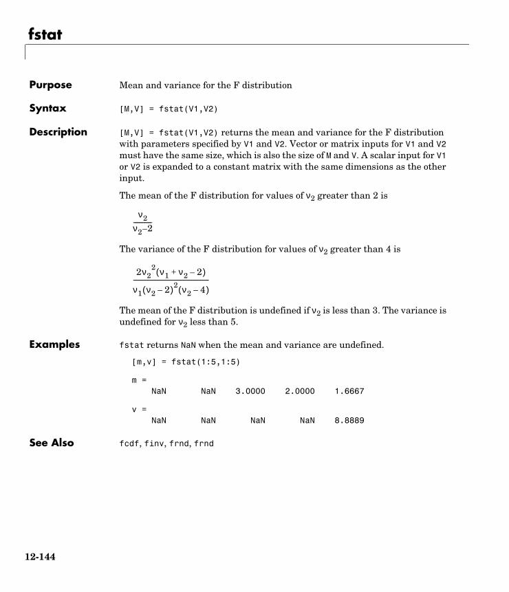
fstat
12fstatPurpose Mean and variance for the F distribution
Syntax [M,V] = fstat(V1,V2)
Description [M,V] = fstat(V1,V2) returns the mean and variance for the F distribution with parameters specified by V1 and V2. Vector or matrix inputs for V1 and V2 must have the same size, which is also the size of M and V. A scalar input for V1 or V2 is expanded to a constant matrix with the same dimensions as the other input.
The mean of the F distribution for values of ν2 greater than 2 is
The variance of the F distribution for values of ν2 greater than 4 is
The mean of the F distribution is undefined if ν2 is less than 3. The variance is undefined for ν2 less than 5.
Examples fstat returns NaN when the mean and variance are undefined.
[m,v] = fstat(1:5,1:5)
m =NaN NaN 3.0000 2.0000 1.6667
v =NaN NaN NaN NaN 8.8889
See Also fcdf, finv, frnd, frnd
ν2ν2 2–------------
2ν22 ν1 ν2 2–+( )
ν1 ν2 2–( )2 ν2 4–( )--------------------------------------------------
12-144

fsurfht
12fsurfhtPurpose Interactive contour plot of a function
Syntax fsurfht('fun',xlims,ylims)fsurfht('fun',xlims,ylims,p1,p2,p3,p4,p5)
Description fsurfht('fun',xlims,ylims) is an interactive contour plot of the function specified by the text variable fun. The x-axis limits are specified by xlims in the form [xmin xmax], and the y-axis limits are specified by ylims in the form [ymin ymax].
fsurfht('fun',xlims,ylims,p1,p2,p3,p4,p5) allows for five optional parameters that you can supply to the function fun.
The intersection of the vertical and horizontal reference lines on the plot defines the current x-value and y-value. You can drag these reference lines and watch the calculated z-values (at the top of the plot) update simultaneously. Alternatively, you can type the x-value and y-value into editable text fields on the x-axis and y-axis.
Example Plot the Gaussian likelihood function for the gas.mat data.
load gas
Create a function containing the following commands, and name it gauslike.m.
function z = gauslike(mu,sigma,p1)n = length(p1);z = ones(size(mu));for i = 1:nz = z .* (normpdf(p1(i),mu,sigma));end
The gauslike function calls normpdf, treating the data sample as fixed and the parameters µ and σ as variables. Assume that the gas prices are normally distributed, and plot the likelihood surface of the sample.
fsurfht('gauslike',[112 118],[3 5],price1)
12-145

fsurfht
The sample mean is the x-value at the maximum, but the sample standard deviation is not the y-value at the maximum.
mumax = mean(price1)
mumax =
115.1500
sigmamax = std(price1)*sqrt(19/20)
sigmamax =
3.7719
12-146

fullfact
12fullfactPurpose Full-factorial experimental design
Syntax design = fullfact(levels)
Description design = fullfact(levels) give the factor settings for a full factorial design. Each element in the vector levels specifies the number of unique values in the corresponding column of design.
For example, if the first element of levels is 3, then the first column of design contains only integers from 1 to 3.
Example If levels = [2 4], fullfact generates an eight-run design with two levels in the first column and four in the second column.
d = fullfact([2 4])
d = 1 1 2 1 1 2 2 2 1 3 2 3 1 4 2 4
See Also ff2n, dcovary, daugment, cordexch
12-147

gamcdf
12gamcdfPurpose Gamma cumulative distribution function (cdf)
Syntax P = gamcdf(X,A,B)
Description gamcdf(X,A,B) computes the gamma cdf at each of the values in X using the corresponding parameters in A and B. Vector or matrix inputs for X, A, and B must all be the same size. A scalar input is expanded to a constant matrix with the same dimensions as the other inputs. The parameters in A and B must be positive.
The gamma cdf is
The result, p, is the probability that a single observation from a gamma distribution with parameters a and b will fall in the interval [0 x].
gammainc is the gamma distribution with b fixed at 1.
Examples a = 1:6;b = 5:10;prob = gamcdf(a.∗ b,a,b)
prob =
0.6321 0.5940 0.5768 0.5665 0.5595 0.5543
The mean of the gamma distribution is the product of the parameters, ab. In this example, the mean approaches the median as it increases (i.e., the distribution becomes more symmetric).
See Also cdf, gamfit, gaminv, gamlike, gampdf, gamrnd, gamstat
p F x a b,( ) 1
baΓ a( )------------------ ta 1– e
tb---–
td0
x
∫= =
12-148

gamfit
12gamfitPurpose Parameter estimates and confidence intervals for gamma distributed data
Syntax phat = gamfit(x)[phat,pci] = gamfit(x)[phat,pci] = gamfit(x,alpha)
Description phat = gamfit(x) returns the maximum likelihood estimates (MLEs) for the parameters of the gamma distribution given the data in vector x.
[phat,pci] = gamfit(x) returns MLEs and 95% percent confidence intervals. The first row of pci is the lower bound of the confidence intervals; the last row is the upper bound.
[phat,pci] = gamfit(x,alpha) returns 100(1-alpha)% confidence intervals. For example, alpha = 0.01 yields 99% confidence intervals.
Example Note that the 95% confidence intervals in the example below bracket the true parameter values of 2 and 4.
a = 2; b = 4;r = gamrnd(a,b,100,1);[p,ci] = gamfit(r)
p = 2.1990 3.7426
ci = 1.6840 2.8298 2.7141 4.6554
Reference [1] Hahn, G. J. and S.S. Shapiro. Statistical Models in Engineering. John Wiley & Sons, New York. 1994. p. 88.
See Also gamcdf, gaminv, gamlike, gampdf, gamrnd, gamstat, betafit, binofit, expfit, normfit, poissfit, unifit, weibfit
12-149

gaminv
12gaminvPurpose Inverse of the gamma cumulative distribution function (cdf)
Syntax X = gaminv(P,A,B)
Description X = gaminv(P,A,B) computes the inverse of the gamma cdf with parameters A and B for the corresponding probabilities in P. Vector or matrix inputs for P, A, and B must all be the same size. A scalar input is expanded to a constant matrix with the same dimensions as the other inputs. The parameters in A and B must all be positive, and the values in P must lie on the interval [0 1].
The gamma inverse function in terms of the gamma cdf is
where
Algorithm There is no known analytical solution to the integral equation above. gaminv uses an iterative approach (Newton’s method) to converge on the solution.
Examples This example shows the relationship between the gamma cdf and its inverse function.
a = 1:5;b = 6:10;x = gaminv(gamcdf(1:5,a,b),a,b)
x = 1.0000 2.0000 3.0000 4.0000 5.0000
See Also gamcdf, gamfit, gamlike, gampdf, gamrnd, gamstat, icdf
x F 1– p a b,( ) x:F x a b,( ) p={ }= =
p F x a b,( ) 1
baΓ a( )------------------ ta 1– e
tb---–
td0
x
∫= =
12-150

gamlike
12gamlikePurpose Negative gamma log-likelihood function
Syntax logL = gamlike(params,data)[logL,avar] = gamlike(params,data)
Description logL = gamlike(params,data) returns the negative of the gamma log-likelihood function for the parameters, params, given data. The length of output vector logL is the length of vector data.
[logL,avar] = gamlike(params,data) also returns avar, which is the asymptotic variance-covariance matrix of the parameter estimates when the values in params are the maximum likelihood estimates. avar is the inverse of Fisher's information matrix. The diagonal elements of avar are the asymptotic variances of their respective parameters.
gamlike is a utility function for maximum likelihood estimation of the gamma distribution. Since gamlike returns the negative gamma log-likelihood function, minimizing gamlike using fminsearch is the same as maximizing the likelihood.
Example This example continues the example for gamfit.
a = 2; b = 3;r = gamrnd(a,b,100,1);[logL,info] = gamlike([2.1990 2.8069],r)
logL =
267.5585
info =
0.0690 -0.0790 -0.0790 0.1220
See Also betalike, gamcdf, gamfit, gaminv, gampdf, gamrnd, gamstat, mle, normlike, weiblike
12-151

gampdf
12gampdfPurpose Gamma probability density function (pdf)
Syntax Y = gampdf(X,A,B)
Description gampdf(X,A,B) computes the gamma pdf at each of the values in X using the corresponding parameters in A and B. Vector or matrix inputs for X, A, and B must all be the same size. A scalar input is expanded to a constant matrix with the same dimensions as the other inputs. The parameters in A and B must all be positive, and the values in X must lie on the interval [0 ∞).
The gamma pdf is
The gamma probability density function is useful in reliability models of lifetimes. The gamma distribution is more flexible than the exponential distribution in that the probability of a product surviving an additional period may depend on its current age. The exponential and χ2 functions are special cases of the gamma function.
Examples The exponential distribution is a special case of the gamma distribution.
mu = 1:5;y = gampdf(1,1,mu)
y = 0.3679 0.3033 0.2388 0.1947 0.1637
y1 = exppdf(1,mu)
y1 = 0.3679 0.3033 0.2388 0.1947 0.1637
See Also gamcdf, gamfit, gaminv, gamlike, gamrnd, gamstat, pdf
y f x a b,( ) 1
baΓ a( )------------------xa 1– e
xb---–
= =
12-152

gamrnd
12gamrndPurpose Random numbers from the gamma distribution
Syntax R = gamrnd(A,B)R = gamrnd(A,B,m)R = gamrnd(A,B,m,n)
Description R = gamrnd(A,B) generates gamma random numbers with parameters A and B. Vector or matrix inputs for A and B must have the same size, which is also the size of R. A scalar input for A or B is expanded to a constant matrix with the same dimensions as the other input.
R = gamrnd(A,B,m) generates gamma random numbers with parameters A and B, where m is a 1-by-2 vector that contains the row and column dimensions of R.
R = gamrnd(A,B,m,n) generates gamma random numbers with parameters A and B, where scalars m and n are the row and column dimensions of R.
Examples n1 = gamrnd(1:5,6:10)
n1 = 9.1132 12.8431 24.8025 38.5960 106.4164
n2 = gamrnd(5,10,[1 5])
n2 = 30.9486 33.5667 33.6837 55.2014 46.8265
n3 = gamrnd(2:6,3,1,5)
n3 = 12.8715 11.3068 3.0982 15.6012 21.6739
See Also gamcdf, gamfit, gaminv, gamlike, gampdf, gamstat
12-153

gamstat
12gamstatPurpose Mean and variance for the gamma distribution
Syntax [M,V] = gamstat(A,B)
Description [M,V] = gamstat(A,B) returns the mean and variance for the gamma distribution with parameters specified by A and B. Vector or matrix inputs for A and B must have the same size, which is also the size of M and V. A scalar input for A or B is expanded to a constant matrix with the same dimensions as the other input.
The mean of the gamma distribution with parameters a and b is ab. The variance is ab2.
Examples [m,v] = gamstat(1:5,1:5)
m = 1 4 9 16 25
v = 1 8 27 64 125
[m,v] = gamstat(1:5,1./(1:5))
m = 1 1 1 1 1
v = 1.0000 0.5000 0.3333 0.2500 0.2000
See Also gamcdf, gamfit, gaminv, gamlike, gampdf, gamrnd
12-154

geocdf
12geocdfPurpose Geometric cumulative distribution function (cdf)
Syntax Y = geocdf(X,P)
Description geocdf(X,P) computes the geometric cdf at each of the values in X using the corresponding probabilities in P. Vector or matrix inputs for X and P must be the same size. A scalar input is expanded to a constant matrix with the same dimensions as the other input. The parameters in P must lie on the interval [0 1].
The geometric cdf is
where .
The result, y, is the probability of observing up to x trials before a success, when the probability of success in any given trial is p.
Examples Suppose you toss a fair coin repeatedly. If the coin lands face up (heads), that is a success. What is the probability of observing three or fewer tails before getting a heads?
p = geocdf(3,0.5)
p = 0.9375
See Also cdf, geoinv, geopdf, geornd, geostat
y F x p( ) pqi
i 0=
floor x( )
∑= =
q 1 p–=
12-155

geoinv
12geoinvPurpose Inverse of the geometric cumulative distribution function (cdf)
Syntax X = geoinv(Y,P)
Description X = geoinv(Y,P) returns the smallest positive integer X such that the geometric cdf evaluated at X is equal to or exceeds Y. You can think of Y as the probability of observing X successes in a row in independent trials where P is the probability of success in each trial.
Vector or matrix inputs for P and Y must have the same size, which is also the size of X. A scalar input for P and Y is expanded to a constant matrix with the same dimensions as the other input. The values in P and Y must lie on the interval [0 1].
Examples The probability of correctly guessing the result of 10 coin tosses in a row is less than 0.001 (unless the coin is not fair).
psychic = geoinv(0.999,0.5)
psychic =
9
The example below shows the inverse method for generating random numbers from the geometric distribution.
rndgeo = geoinv(rand(2,5),0.5)
rndgeo =
0 1 3 1 0 0 1 0 2 0
See Also geocdf, geopdf, geornd, geostat, icdf
12-156

geomean
12geomeanPurpose Geometric mean of a sample
Syntax m = geomean(X)
Description geomean calculates the geometric mean of a sample. For vectors, geomean(x) is the geometric mean of the elements in x. For matrices, geomean(X) is a row vector containing the geometric means of each column.
The geometric mean is
Examples The sample average is greater than or equal to the geometric mean.
x = exprnd(1,10,6);geometric = geomean(x)
geometric =
0.7466 0.6061 0.6038 0.2569 0.7539 0.3478
average = mean(x)
average =
1.3509 1.1583 0.9741 0.5319 1.0088 0.8122
See Also mean, median, harmmean, trimmean
m xi
i 1=
n
∏
1n---
=
12-157

geopdf
12geopdfPurpose Geometric probability density function (pdf)
Syntax Y = geopdf(X,P)
Description geocdf(X,P) computes the geometric pdf at each of the values in X using the corresponding probabilities in P. Vector or matrix inputs for X and P must be the same size. A scalar input is expanded to a constant matrix with the same dimensions as the other input. The parameters in P must lie on the interval [0 1].
The geometric pdf is
where .
Examples Suppose you toss a fair coin repeatedly. If the coin lands face up (heads), that is a success. What is the probability of observing exactly three tails before getting a heads?
p = geopdf(3,0.5)
p = 0.0625
See Also geocdf, geoinv, geornd, geostat, pdf
y f x p( ) pqxI 0 1 K, ,( ) x( )= =
q 1 p–=
12-158

geornd
12georndPurpose Random numbers from the geometric distribution
Syntax R = geornd(P)R = geornd(P,m)R = geornd(P,m,n)
Description The geometric distribution is useful when you want to model the number of successive failures preceding a success, where the probability of success in any given trial is the constant P.
R = geornd(P) generates geometric random numbers with probability parameter P. The size of R is the size of P.
R = geornd(P,m) generates geometric random numbers with probability parameter P, where m is a 1-by-2 vector that contains the row and column dimensions of R.
R = geornd(P,m,n) generates geometric random numbers with probability parameter P, where scalars m and n are the row and column dimensions of R.
The parameters in P must lie on the interval [0 1].
Examples r1 = geornd(1 ./ 2.^(1:6))
r1 = 2 10 2 5 2 60
r2 = geornd(0.01,[1 5])
r2 = 65 18 334 291 63
r3 = geornd(0.5,1,6)
r3 = 0 7 1 3 1 0
See Also geocdf, geoinv, geopdf, geostat
12-159

geostat
12geostatPurpose Mean and variance for the geometric distribution
Syntax [M,V] = geostat(P)
Description [M,V] = geostat(P) returns the mean and variance for the geometric distribution with parameters specified by P.
The mean of the geometric distribution with parameter p is q/p, where q = 1-p. The variance is q/p2.
Examples [m,v] = geostat(1./(1:6))
m =0 1.0000 2.0000 3.0000 4.0000 5.0000
v =0 2.0000 6.0000 12.0000 20.0000 30.0000
See Also geocdf, geoinv, geopdf, geornd
12-160

gline
12glinePurpose Interactively draw a line in a figure
Syntax gline(fig)h = gline(fig)gline
Description gline(fig) allows you to draw a line segment in the figure fig by clicking the pointer at the two end-points. A rubber band line tracks the pointer movement.
h = gline(fig) returns the handle to the line in h.
gline with no input arguments draws in the current figure.
See Also refline, gname
12-161
glmdemo
12glmdemoPurpose Demo of generalized linear models
Syntax glmdemo
Description glmdemo begins a slide show demonstration of generalized linear models. The slides indicate when generalized linear models are useful, how to fit generalized linear models using the glmfit function, and how to make predictions using the glmval function.
Note To run this demo from the command line, type playshow glmdemo.
See Also glmfit, glmval
12-162

glmfit
12glmfitPurpose Generalized linear model fitting
Syntax b = glmfit(X,Y,'distr')b = glmfit(X,Y,'distr','link','estdisp',offset,pwts,'const')[b,dev,stats] = glmfit(...)
Description b = glmfit(x,y,'distr') fits the generalized linear model for response Y, predictor variable matrix X, and distribution 'distr'. The following distributions are available: 'binomial', 'gamma', 'inverse gaussian', 'lognormal', 'normal' (the default), and 'poisson'. In most cases Y is a vector of response measurements, but for the binomial distribution Y is a two-column array having the measured number of counts in the first column and the number of trials (the binomial N parameter) in the second column. X is a matrix having the same number of rows as Y and containing the values of the predictor variables for each observation. The output b is a vector of coefficient estimates. This syntax uses the canonical link (see below) to relate the distribution parameter to the predictors.
b = glmfit(x,y,'distr','link','estdisp',offset,pwts,'const')provides additional control over the fit. The 'link' argument specifies the relationship between the distribution parameter (µ) and the fitted linear combination of predictor variables (xb). In most cases 'link' is one of the following:
'link' Meaning Default (Canonical) Link
'identity' µ = xb 'normal'
'log' log(µ) = xb 'poisson'
'logit' log(µ / (1-µ)) = xb 'binomial'
'probit' norminv(µ) = xb
'comploglog' log(-log(1-µ)) = xb
'logloglink' log(-log(µ)) = xb
'reciprocal' 1/µ = xb 'gamma'
p (a number) µp = xb 'inverse gaussian' (with p=-2)
12-163

glmfit
Alternatively, you can write functions to define your own custom link. You specify the link argument as a three-element cell array containing functions that define the link function, its derivative, and its inverse. For example, suppose you want to define a reciprocal square root link using inline functions. You could define the variable mylinks to use as your 'link' argument by writing:
FL = inline('x.^-.5')FD = inline('-.5*x.^-1.5')FI = inline('x.^-2')mylinks = {FL FI FD}
Alternatively, you could define functions named FL, FD, and FI in their own M-files, and then specify mylinks in the form
mylinks = {@FL @FD @FI}
The 'estdisp' argument can be 'on' to estimate a dispersion parameter for the binomial or Poisson distribution, or 'off' (the default) to use the theoretical value of 1.0 for those distributions. The glmfit function always estimates dispersion parameters for other distributions.
The offset and pwts parameters can be vectors of the same length as Y, or can be omitted (or specified as an empty vector). The offset vector is a special predictor variable whose coefficient is known to be 1.0. As an example, suppose that you are modeling the number of defects on various surfaces, and you want to construct a model in which the expected number of defects is proportional to the surface area. You might use the number of defects as your response, along with the Poisson distribution, the log link function, and the log surface area as an offset.
The pwts argument is a vector of prior weights. As an example, if the response value Y(i) is the average of f(i) measurements, you could use f as a vector of prior weights.
The 'const' argument can be 'on' (the default) to estimate a constant term, or 'off' to omit the constant term. If you want the constant term, use this argument rather than specifying a column of ones in the X matrix.
[b,dev,stats] = glmfit(...) returns the additional outputs dev and stats. dev is the deviance at the solution vector. The deviance is a generalization of the residual sum of squares. It is possible to perform an analysis of deviance to
12-164

glmfit
compare several models, each a subset of the other, and to test whether the model with more terms is significantly better than the model with fewer terms.
stats is a structure with the following fields:
• stats.dfe = degrees of freedom for error
• stats.s = theoretical or estimated dispersion parameter
• stats.sfit = estimated dispersion parameter
• stats.estdisp = 1 if dispersion is estimated, 0 if fixed
• stats.beta = vector of coefficient estimates (same as b)
• stats.se = vector of standard errors of the coefficient estimates b
• stats.coeffcorr = correlation matrix for b
• stats.t = t statistics for b
• stats.p = p-values for b
• stats.resid = vector of residuals
• stats.residp = vector of Pearson residuals
• stats.residd = vector of deviance residuals
• stats.resida = vector of Anscombe residuals
If you estimate a dispersion parameter for the binomial or Poisson distribution, then stats.s is set equal to stats.sfit. Also, the elements of stats.se differ by the factor stats.s from their theoretical values.
Example We have data on cars weighing between 2100 and 4300 pounds. For each car weight we have the total number of cars of that weight, and the number that can be considered to get “poor mileage” according to some test. For example, 8 out of 21 cars weighing 3100 pounds get poor mileage according to a measurement of the miles they can travel on a gallon of gasoline.
w = (2100:200:4300)';poor = [1 2 0 3 8 8 14 17 19 15 17 21]';total = [48 42 31 34 31 21 23 23 21 16 17 21]';
We can compare several fits to these data. First, let’s try fitting logit and probit models:
[bl,dl,sl] = glmfit(w,[poor total],'binomial');[bp,dp,sp] = glmfit(w,[poor total],'binomial','probit');
12-165

glmfit
dldl = 6.4842
dpdp = 7.5693
The deviance for the logit model is smaller than for the probit model. Although this is not a formal test, it leads us to prefer the logit model.
We can do a formal test comparing two logit models. We already fit one model using w as a linear predictor. Let’s fit another logit model using both linear and squared terms in w. If there is no true effect for the squared term, the difference in their deviances should be small compared with a chi-square distribution having one degree of freedom.
[b2,d2,s2] = glmfit([w w.^2],[poor total],'binomial')
dl-d2
ans = 0.7027
chi2cdf(dl-d2,1)
ans = 0.5981
A difference of 0.7072 is not at all unusual for a chi-square distribution with one degree of freedom, so the quadratic model does not give a significantly better fit than the simpler linear model.
The following are the coefficient estimates, their standard errors, t-statistics, and p-values for the linear model:
[b sl.se sl.t sl.p]
ans =
-13.3801 1.3940 -9.5986 0.0000 0.0042 0.0004 9.4474 0.0000
12-166

glmfit
This shows that we cannot simplify the model any further. Both the intercept and slope coefficients are significantly different from 0, as indicated by p-values that are 0.0000 to four decimal places.
See Also glmval, glmdemo, nlinfit, regress, regstats
References [1] Dobson, A. J. An Introduction to Generalized Linear Models. 1990, CRC Press.
[2] MuCullagh, P. and J. A. Nelder. Generalized Linear Models. 2nd edition, 1990, Chapman and Hall.
12-167

glmval
12glmvalPurpose Compute predictions for generalized linear model
Syntax yfit = glmval(b,X,'link')[yfit,dlo,dhi] = glmval(b,X,'link',stats,clev)[yfit,dlo,dhi] = glmval(b,X,'link',stats,clev,N,offset,'const')
Description yfit = glmval(b,X,'link') computes the predicted distribution parameters for observations with predictor values X using the coefficient vector b and link function 'link'. Typically, b is a vector of coefficient estimates computed by the glmfit function. The value of 'link' must be the same as that used in glmfit. The result yfit is the value of the inverse of the link function at the linear combination X*b.
[yfit,dlo,dhi] = glmval(b,X,'link',stats,clev) returns confidence bounds for the predicted values when you supply the stats structure returned from glmfit, and optionally specify a confidence level as the clev argument. (The default confidence level is 0.95 for 95% confidence.) The interval [yfit-dlo, yfit+dhi] is a confidence bound for the true parameter value at the specified X values.
[yhat,dlo,dhi] = glmval(beta,X,'link',stats,clev,N,offset,'const')specifies three additional arguments that may be needed if you used certain arguments to glmfit. If you fit a binomial distribution using glmfit, specify N as the value of the binomial N parameter for the predictions. If you included an offset variable, specify offset as the new value of this variable. Use the same 'const' value ('on' or 'off') that you used with glmfit.
Example Let's model the number of cars with poor gasoline mileage using the binomial distribution. First we use the binomial distribution with the default logit link to model the probability of having poor mileage as a function of the weight and squared weight of the cars. Then we compute a vector wnew of new car weights at which we want to make predictions. Next we compute the expected number of cars, out of a total of 30 cars of each weight, that would have poor mileage. Finally we graph the predicted values and 95% confidence bounds as a function of weight.
w = [2100 2300 2500 2700 2900 3100 3300 3500 3700 3900 4100 4300]';poor = [1 2 0 3 8 8 14 17 19 15 17 21]';total = [48 42 31 34 31 21 23 23 21 16 17 21]';
12-168

glmval
[b2,d2,s2] = glmfit([w w.^2],[poor total],'binomial')wnew = (3000:100:4000)';[yfit,dlo,dhi] = glmval(b2,[wnew wnew.^2],'logit',s2,0.95,30)errorbar(wnew,yfit,dlo,dhi);
See Also glmfit, glmdemo
2800 3000 3200 3400 3600 3800 4000 42005
10
15
20
25
30
12-169

gname
12gnamePurpose Label plotted points with their case names or case number
Syntax gname('cases')gnameh = gname('cases',line_handle)
Description gname('cases') displays a figure window, displays cross-hairs, and waits for a mouse button or keyboard key to be pressed. Position the cross-hair with the mouse and click once near each point to label that point. Input 'cases' is a string matrix with each row the case name of a data point. You can also click and drag a selection rectangle to label all points within the rectangle. When you are done, press the Enter or Escape key.
gname with no arguments labels each case with its case number.
h = gname('cases',line_handle) returns a vector of handles to the text objects on the plot. Use the scalar line_handle to identify the correct line if there is more than one line object on the plot.
You can use gname to label plots created by the plot, scatter, gscatter, plotmatrix, and gplotmatrix functions.
Example Let’s use the city ratings data sets to find out which cities are the best and worst for education and the arts. We create a graph, call the gname function, and click on the points at the extreme left and at the top.
load citieseducation = ratings(:,6);arts = ratings(:,7);plot(education,arts,'+')gname(names)
12-170

gname
See Also gplotmatrix, gscatter, gtext, plot, plotmatrix, scatter
1500 2000 2500 3000 3500 40000
1
2
3
4
5
6x 10⁴
Pascagoula, MS
New York, NY
12-171

gplotmatrix
12gplotmatrixPurpose Plot matrix of scatter plots by group
Syntax gplotmatrix(x,y,g)gplotmatrix(x,y,g,'clr','sym',siz)gplotmatrix(x,y,g,'clr','sym',siz,'doleg')gplotmatrix(x,y,g,'clr','sym',siz,'doleg','dispopt')gplotmatrix(x,y,g,'clr','sym',siz,'doleg','dispopt','xnam','ynam')[h,ax,bigax] = gplotmatrix(...)
Description gplotmatrix(x,y,g) creates a matrix of scatter plots. Each individual set of axes in the resulting figure contains a scatter plot of a column of x against a column of y. All plots are grouped by the grouping variable g.
x and y are matrices with the same number of rows. If x has p columns and y has q columns, the figure contains a p-by-q matrix of scatter plots. If you omit y or specify it as the empty matrix, [], gplotmatrix creates a square matrix of scatter plots of columns of x against each other.
g is a grouping variable that can be a vector, string array, or cell array of strings. g must have the same number of rows as x and y. Points with the same value of g are placed in the same group, and appear on the graph with the same marker and color. Alternatively, g can be a cell array containing several grouping variables (such as {G1 G2 G3}); in that case, observations are in the same group if they have common values of all grouping variables.
gplotmatrix(x,y,g,'clr','sym',siz) specifies the color, marker type, and size for each group. clr is a string array of colors recognized by the plot function. The default is 'clr' = 'bgrcmyk'. 'sym' is a string array of symbols recognized by the plot command, with the default value '.'. siz is a vector of sizes, with the default determined by the 'defaultlinemarkersize' property. If you do not specify enough values for all groups, gplotmatrix cycles through the specified values as needed.
gplotmatrix(x,y,g,'clr','sym',siz,'doleg') controls whether a legend is displayed on the graph ('doleg' = 'on', the default) or not ('doleg' = 'off').
gplotmatrix(x,y,g,'clr','sym',siz,'doleg','dispopt') controls what appears along the diagonal of a plot matrix of x versus x. Allowable values are
12-172

gplotmatrix
'none' to leave the diagonals blank, 'hist' (the default) to plot histograms, or 'variable' to write the variable names.
gplotmatrix(x,y,g,'clr','sym',siz,'doleg','dispopt','xnam','ynam')specifies the names of the columns in the x and y arrays. These names are used to label the x- and y-axes. 'xnam' and 'ynam' must be character arrays with one row for each column of x and y, respectively.
[h,ax,bigax] = gplotmatrix(...) returns three arrays of handles. h is an array of handles to the lines on the graphs. ax is a matrix of handles to the axes of the individual plots. bigax is a handle to big (invisible) axes framing the entire plot matrix. These are left as the current axes, so a subsequent title, xlabel, or ylabel command will produce labels that are centered with respect to the entire plot matrix.
Example Load the cities data. The ratings array has ratings of the cities in nine categories (category names are in the array categories). group is a code whose value is 2 for the largest cities. We can make scatter plots of the first three categories against the other four, grouped by the city size code.
load discrimgplotmatrix(ratings(:,1:3),ratings(:,4:7),group)
The output figure (not shown) has an array of graphs with each city group represented by a different color. The graphs are a little easier to read if we specify colors and plotting symbols, label the axes with the rating categories, and move the legend off the graphs.
gplotmatrix(ratings(:,1:3),ratings(:,4:7),group,...'br','.o',[],'on','',categories(1:3,:),...categories(4:7,:))
12-173

gplotmatrix
See Also grpstats, gscatter, plotmatrix
0 2000 4000 6000 8000health
0.5 1 1.5 2
x 104housing
200 400 600 8000
2
4
x 104
climate
arts
2000250030003500
educ
atio
n
2000
4000
6000
8000tr
ansp
orta
tion
5001000150020002500
crim
e
12
12-174

grpstats
12grpstatsPurpose Summary statistics by group
Syntax means = grpstats(X,group)[means,sem,counts,name] = grpstats(X,group)grpstats(x,group,alpha)
Description means = grpstats(X,group) returns the means of each column of X by group, where X is a matrix of observations. group is an array that defines the grouping such that two elements of X are in the same group if their corresponding group values are the same. The grouping variable group can be a vector, string array, or cell array of strings. It can also be a cell array containing several grouping variables (such as {G1 G2 G3}); in that case observations are in the same group if they have common values of all grouping variables.
[means,sem,counts,name] = grpstats(x,group,alpha) supplies the standard error of the mean in sem, the number of elements in each group in counts, and the name of each group in name. name is useful to identify and label the groups when the input group values are not simple group numbers.
grpstats(x,group,alpha) plots 100(1-alpha)% confidence intervals around each mean.
Example We assign 100 observations to one of four groups. For each observation we measure five quantities with true means from 1 to 5. grpstats allows us to compute the means for each group.
group = unidrnd(4,100,1);true_mean = 1:5;true_mean = true_mean(ones(100,1),:);x = normrnd(true_mean,1);means = grpstats(x,group)
means =
0.7947 2.0908 2.8969 3.6749 4.6555 0.9377 1.7600 3.0285 3.9484 4.8169 1.0549 2.0255 2.8793 4.0799 5.3740 0.7107 1.9264 2.8232 3.8815 4.9689
See Also tabulate, crosstab
12-175

gscatter
12gscatterPurpose Scatter plot by group
Syntax gscatter(x,y,g)gscatter(x,y,g,'clr','sym',siz)gscatter(x,y,g,'clr','sym',siz,'doleg')gscatter(x,y,g,'clr','sym',siz,'doleg','xnam','ynam')h = gscatter(...)
Description gscatter(x,y,g) creates a scatter plot of x and y, grouped by g, where x and y are vectors with the same size and g can be a vector, string array, or cell array of strings. Points with the same value of g are placed in the same group, and appear on the graph with the same marker and color. Alternatively, g can be a cell array containing several grouping variables (such as {G1 G2 G3}); in that case, observations are in the same group if they have common values of all grouping variables.
gscatter(x,y,g,'clr','sym',siz) specifies the color, marker type, and size for each group. 'clr' is a string array of colors recognized by the plot function. The default is 'clr' = 'bgrcmyk'. 'sym' is a string array of symbols recognized by the plot command, with the default value '.'. siz is a vector of sizes, with the default determined by the 'defaultlinemarkersize' property. If you do not specify enough values for all groups, gscatter cycles through the specified values as needed.
gscatter(x,y,g,'clr','sym',siz,'doleg') controls whether a legend is displayed on the graph ('doleg' = 'on', the default) or not ('doleg' = 'off').
gscatter(x,y,g,'clr','sym',siz,'doleg','xnam','ynam') specifies the name to use for the x-axis and y-axis labels. If the x and y inputs are simple variable names and xnam and ynam are omitted, gscatter labels the axes with the variable names.
h = gscatter(...) returns an array of handles to the lines on the graph.
Example Load the cities data and look at the relationship between the ratings for climate (first column) and housing (second column) grouped by city size. We’ll also specify the colors and plotting symbols.
load discrim
12-176
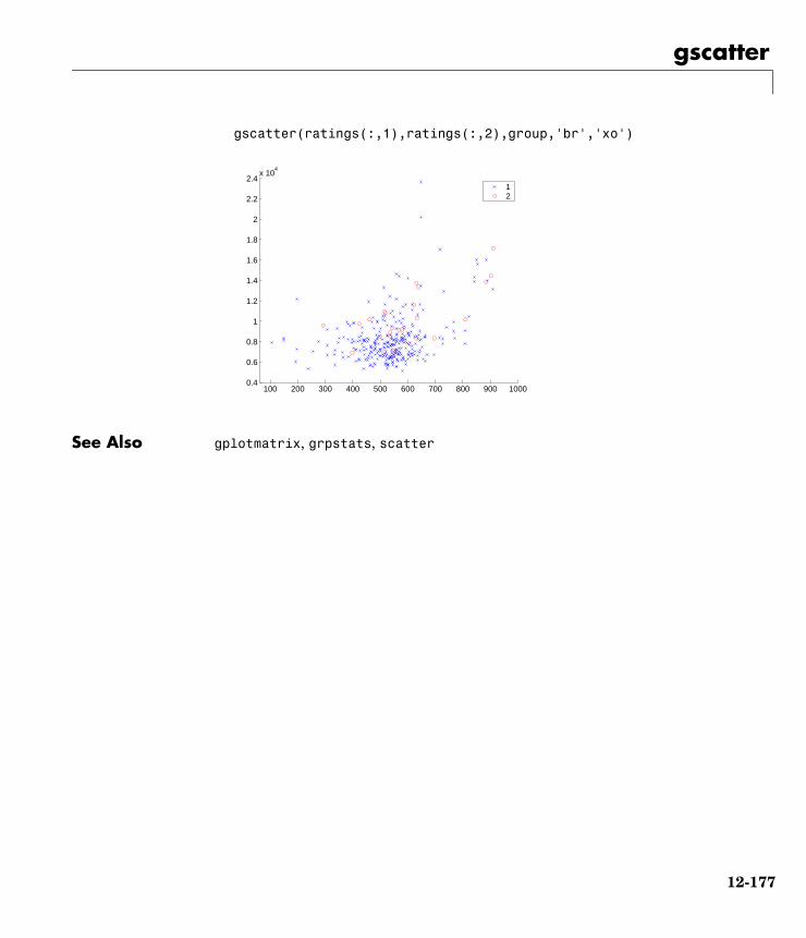
gscatter
gscatter(ratings(:,1),ratings(:,2),group,'br','xo')
See Also gplotmatrix, grpstats, scatter
100 200 300 400 500 600 700 800 900 10000.4
0.6
0.8
1
1.2
1.4
1.6
1.8
2
2.2
2.4x 10
4
12
12-177

harmmean
12harmmeanPurpose Harmonic mean of a sample of data
Syntax m = harmmean(X)
Description m = harmmean(X) calculates the harmonic mean of a sample. For vectors, harmmean(x) is the harmonic mean of the elements in x. For matrices, harmmean(X) is a row vector containing the harmonic means of each column.
The harmonic mean is
Examples The sample average is greater than or equal to the harmonic mean.
x = exprnd(1,10,6);harmonic = harmmean(x)
harmonic =
0.3382 0.3200 0.3710 0.0540 0.4936 0.0907
average = mean(x)
average =
1.3509 1.1583 0.9741 0.5319 1.0088 0.8122
See Also mean, median, geomean, trimmean
m n
1xi----
i 1=
n
∑
---------------=
12-178

hist
12histPurpose Plot histograms
Syntax hist(y)hist(y,nb)hist(y,x)[n,x] = hist(y,...)
Description hist(y) draws a 10-bin histogram for the data in vector y. The bins are equally spaced between the minimum and maximum values in y.
hist(y,nb) draws a histogram with nb bins.
hist(y,x) draws a histogram using the bins in the vector x.
[n,x] = hist(y,...) do not draw graphs, but return vectors n and x containing the frequency counts and the bin locations such that bar(x,n) plots the histogram. This is useful in situations where more control is needed over the appearance of a graph, for example, to combine a histogram into a more elaborate plot statement.
The hist function is a part of the standard MATLAB language.
Examples Generate bell-curve histograms from Gaussian data.
x = -2.9:0.1:2.9;y = normrnd(0,1,1000,1);hist(y,x)
-3 -2 -1 0 1 2 30
10
20
30
40
50
12-179

histfit
12histfitPurpose Histogram with superimposed normal density
Syntax histfit(data)histfit(data,nbins)h = histfit(data,nbins)
Description histfit(data,nbins) plots a histogram of the values in the vector data using nbins bars in the histogram. With nbins is omitted, its value is set to the square root of the number of elements in data.
h = histfit(data,nbins) returns a vector of handles to the plotted lines, where h(1) is the handle to the histogram, h(2) is the handle to the density curve.
Example r = normrnd(10,1,100,1);histfit(r)
See Also hist, normfit
7 8 9 10 11 12 130
5
10
15
20
25
12-180

hougen
12hougenPurpose Hougen-Watson model for reaction kinetics
Syntax yhat = hougen(beta,x)
Description yhat = hougen(beta,x) returns the predicted values of the reaction rate, yhat, as a function of the vector of parameters, beta, and the matrix of data, X. beta must have 5 elements and X must have three columns.
hougen is a utility function for rsmdemo.
The model form is:
Reference [1] Bates, D., and D. Watts. Nonlinear Regression Analysis and Its Applications. Wiley 1988. p. 271–272.
See Also rsmdemo
y�β1x2 x3 β5⁄–
1 β2x1 β3x2 β4x3+ + +-----------------------------------------------------------=
12-181

hygecdf
12hygecdfPurpose Hypergeometric cumulative distribution function (cdf)
Syntax P = hygecdf(X,M,K,N)
Description hygecdf(X,M,K,N) computes the hypergeometric cdf at each of the values in X using the corresponding parameters in M, K, and N. Vector or matrix inputs for X, M, K, and N must all have the same size. A scalar input is expanded to a constant matrix with the same dimensions as the other inputs.
The hypergeometric cdf is
The result, p, is the probability of drawing up to x of a possible K items in N drawings without replacement from a group of M objects.
Examples Suppose you have a lot of 100 floppy disks and you know that 20 of them are defective. What is the probability of drawing zero to two defective floppies if you select 10 at random?
p = hygecdf(2,100,20,10)
p = 0.6812
See Also cdf, hygeinv, hygepdf, hygernd, hygestat
p F x M K N, ,( )
Ki
M K–
N i–
MN
-------------------------------
i 0=
x
∑= =
12-182

hygeinv
12hygeinvPurpose Inverse of the hypergeometric cumulative distribution function (cdf)
Syntax X = hygeinv(P,M,K,N)
Description hygeinv(P,M,K,N) returns the smallest integer X such that the hypergeometric cdf evaluated at X equals or exceeds P. You can think of P as the probability of observing X defective items in N drawings without replacement from a group of M items where K are defective.
Examples Suppose you are the Quality Assurance manager for a floppy disk manufacturer. The production line turns out floppy disks in batches of 1,000. You want to sample 50 disks from each batch to see if they have defects. You want to accept 99% of the batches if there are no more than 10 defective disks in the batch. What is the maximum number of defective disks should you allow in your sample of 50?
x = hygeinv(0.99,1000,10,50)
x = 3
What is the median number of defective floppy disks in samples of 50 disks from batches with 10 defective disks?
x = hygeinv(0.50,1000,10,50)
x = 0
See Also hygecdf, hygepdf, hygernd, hygestat, icdf
12-183

hygepdf
12hygepdfPurpose Hypergeometric probability density function (pdf)
Syntax Y = hygepdf(X,M,K,N)
Description Y = hygecdf(X,M,K,N) computes the hypergeometric pdf at each of the values in X using the corresponding parameters in M, K, and N. Vector or matrix inputs for X, M, K, and N must all have the same size. A scalar input is expanded to a constant matrix with the same dimensions as the other inputs.
The parameters in M, K, and N must all be positive integers, with N ≤ M. The values in X must be less than or equal to all the parameter values.
The hypergeometric pdf is
The result, y, is the probability of drawing exactly x of a possible K items in n drawings without replacement from a group of M objects.
Examples Suppose you have a lot of 100 floppy disks and you know that 20 of them are defective. What is the probability of drawing 0 through 5 defective floppy disks if you select 10 at random?
p = hygepdf(0:5,100,20,10)
p = 0.0951 0.2679 0.3182 0.2092 0.0841 0.0215
See Also hygecdf, hygeinv, hygernd, hygestat, pdf
y f x M K N, ,( )
Kx M K–
N x–
MN
-------------------------------= =
12-184

hygernd
12hygerndPurpose Random numbers from the hypergeometric distribution
Syntax R = hygernd(M,K,N)R = hygernd(M,K,N,mm)R = hygernd(M,K,N,mm,nn)
Description R = hygernd(M,K,N) generates hypergeometric random numbers with parameters M, K, and N. Vector or matrix inputs for M, K, and N must have the same size, which is also the size of R. A scalar input for M, K, or N is expanded to a constant matrix with the same dimensions as the other inputs.
R = hygernd(M,K,N,mm) generates hypergeometric random numbers with parameters M, K, and N, where mm is a 1-by-2 vector that contains the row and column dimensions of R.
R = hygernd(M,K,N,mm,nn) generates hypergeometric random numbers with parameters M, K, and N, where scalars mm and nn are the row and column dimensions of R.
Examples numbers = hygernd(1000,40,50)
numbers =
1
See Also hygecdf, hygeinv, hygepdf, hygestat
12-185

hygestat
12hygestatPurpose Mean and variance for the hypergeometric distribution
Syntax [MN,V] = hygestat(M,K,N)
Description [MN,V] = hygestat(M,K,N) returns the mean and variance for the hypergeometric distribution with parameters specified by M, K, and N. Vector or matrix inputs for M, K, and N must have the same size, which is also the size of MN and V. A scalar input for M, K, or N is expanded to a constant matrix with the same dimensions as the other inputs.
The mean of the hypergeometric distribution with parameters M, K, and N is NK/M, and the variance is
Examples The hypergeometric distribution approaches the binomial distribution, where p = K / M as M goes to infinity.
[m,v] = hygestat(10.^(1:4),10.^(0:3),9)
m = 0.9000 0.9000 0.9000 0.9000
v = 0.0900 0.7445 0.8035 0.8094
[m,v] = binostat(9,0.1)
m = 0.9000
v = 0.8100
See Also hygecdf, hygeinv, hygepdf, hygernd
N KM-----M K–
M----------------M N–
M 1–----------------
12-186

icdf
12icdfPurpose Inverse of a specified cumulative distribution function (icdf)
Syntax X = icdf('name',P,A1,A2,A3)
Description X = icdf('name',P,A1,A2,A3) returns a matrix of critical values, X, where 'name' is a string containing the name of the distribution. P is a matrix of probabilities, and A, B, and C are matrices of distribution parameters. Depending on the distribution some of the parameters may not be necessary.
Vector or matrix inputs for P, A1, A2, and A3 must all have the same size. A scalar input is expanded to a constant matrix with the same dimensions as the other inputs.
icdf is a utility routine allowing you to access all the inverse cdfs in the Statistics Toolbox using the name of the distribution as a parameter. See “Overview of the Distributions” on page 2-11 for the list of available distributions.
Examples x = icdf('Normal',0.1:0.2:0.9,0,1)
x = -1.2816 -0.5244 0 0.5244 1.2816
x = icdf('Poisson',0.1:0.2:0.9,1:5)
x = 1 1 3 5 8
See Also betainv, binoinv, cdf, chi2inv, expinv, finv, gaminv, geoinv, hygeinv, logninv, nbininv, ncfinv, nctinv, ncx2inv, norminv, pdf, poissinv, random, raylinv, tinv, unidinv, unifinv, weibinv
12-187

inconsistent
12inconsistentPurpose Calculate the inconsistency coefficient of a cluster tree
Syntax Y = inconsistent(Z) Y = inconsistent(Z,d)
Description Y = inconsistent(Z) computes the inconsistency coefficient for each link of the hierarchical cluster tree Z, where Z is an (m-1)-by-3 matrix generated by the linkage function. The inconsistency coefficient characterizes each link in a cluster tree by comparing its length with the average length of other links at the same level of the hierarchy. The higher the value of this coefficient, the less similar the objects connected by the link.
Y = inconsistent(Z,d) computes the inconsistency coefficient for each link in the hierarchical cluster tree Z to depth d, where d is an integer denoting the number of levels of the cluster tree that are included in the calculation. By default, d=2.
The output, Y, is an (m-1)-by-4 matrix formatted as follows.
For each link, k, the inconsistency coefficient is calculated as:
For leaf nodes, nodes that have no further nodes under them, the inconsistency coefficient is set to 0.
Example rand('seed',12);X = rand(10,2);Y = pdist(X);
Column Description
1 Mean of the lengths of all the links included in the calculation.
2 Standard deviation of all the links included in the calculation.
3 Number of links included in the calculation.
4 Inconsistency coefficient.
Y k 4,( ) z k 3,( ) Y k 1,( )–( ) Y k 2,( )⁄=
12-188

inconsistent
Z = linkage(Y,'centroid');W = inconsistent(Z,3)
W =
0.0423 0 1.0000 0 0.1406 0 1.0000 0 0.1163 0.1047 2.0000 0.70710.2101 0 1.0000 00.2054 0.0886 3.0000 0.67920.1742 0.1762 3.0000 0.65680.2336 0.1317 4.0000 0.64080.3081 0.2109 5.0000 0.79890.4610 0.3728 4.0000 0.8004
See Also cluster, cophenet, clusterdata, dendrogram, linkage, pdist, squareform
12-189

iqr
12iqrPurpose Interquartile range (IQR) of a sample
Syntax y = iqr(X)
Description y = iqr(X) computes the difference between the 75th and the 25th percentiles of the sample in X. The IQR is a robust estimate of the spread of the data, since changes in the upper and lower 25% of the data do not affect it.
If there are outliers in the data, then the IQR is more representative than the standard deviation as an estimate of the spread of the body of the data. The IQR is less efficient than the standard deviation as an estimate of the spread when the data is all from the normal distribution.
Multiply the IQR by 0.7413 to estimate σ (the second parameter of the normal distribution.)
Examples This Monte Carlo simulation shows the relative efficiency of the IQR to the sample standard deviation for normal data.
x = normrnd(0,1,100,100);s = std(x);s_IQR = 0.7413 ∗ iqr(x);efficiency = (norm(s - 1)./norm(s_IQR - 1)).^2
efficiency =
0.3297
See Also std, mad, range
12-190

iwishrnd
12iwishrndPurpose Generate inverse Wishart random matrix
Syntax W=iwishrnd(SIGMA,df)W=iwishrnd(SIGMA,df,DI)[W,DI]=iwishrnd(SIGMA,df)
Description W=iwishrnd(SIGMA,df) generates a random matrix W whose inverse has the Wishart distribution with covariance matrix inv(SIGMA) and with df degrees of freedom.
W=iwishrnd(SIGMA,df,DI) expects DI to be the Cholesky factor of the inverse of SIGMA. If you call iwishrnd multiple times using the same value of SIGMA, it's more efficient to supply DI instead of computing it each time.
[W,DI]=iwishrnd(SIGMA,df) returns DI so you can provide it as input in future calls to iwishrnd.
See Also wishrnd
12-191

jbtest
12jbtestPurpose Jarque-Bera test for goodness-of-fit to a normal distribution
Syntax H = jbtest(X)H = jbtest(X,alpha)[H,P,JBSTAT,CV] = jbtest(X,alpha)
Description H = jbtest(X) performs the Jarque-Bera test on the input data vector X and returns H, the result of the hypothesis test. The result is H=1 if we can reject the hypothesis that X has a normal distribution, or H=0 if we cannot reject that hypothesis. We reject the hypothesis if the test is significant at the 5% level.
The Jarque-Bera test evaluates the hypothesis that X has a normal distribution with unspecified mean and variance, against the alternative that X does not have a normal distribution. The test is based on the sample skewness and kurtosis of X. For a true normal distribution, the sample skewness should be near 0 and the sample kurtosis should be near 3. The Jarque-Bera test determines whether the sample skewness and kurtosis are unusually different than their expected values, as measured by a chi-square statistic.
The Jarque-Bera test is an asymptotic test, and should not be used with small samples. You may want to use lillietest in place of jbtest for small samples.
H = jbtest(X,alpha) performs the Jarque-Bera test at the 100*alpha% level rather than the 5% level, where alpha must be between 0 and 1.
[H,P,JBSTAT,CV] = jbtest(X,alpha) returns three additional outputs. P is the p-value of the test, JBSTAT is the value of the test statistic, and CV is the critical value for determining whether to reject the null hypothesis.
Example We can use jbtest to determine if car weights follow a normal distribution.
load carsmall[h,p,j] = jbtest(Weight)
h = 1
p = 0.026718
j =
12-192

jbtest
7.2448
With a p-value of 2.67%, we reject the hypothesis that the distribution is normal. With a log transformation, the distribution becomes closer to normal but is still significantly different at the 5% level.
[h,p,j] = jbtest(log(Weight))
h = 1
p = 0.043474
j = 6.2712
See lillietest for a different test of the same hypothesis.
Reference [1] Judge, G. G., R. C. Hill, W. E. Griffiths, H. Lutkepohl, and T.-C. Lee. Introduction to the Theory and Practice of Econometrics. New York, Wiley.
See Also hist, kstest2, lillietest
12-193

kmeans
12kmeansPurpose K-means clustering
Syntax IDX = kmeans(X,k)[IDX,C] = kmeans(X,k)[IDX,C,sumd] = kmeans(X,k)[IDX,C,sumd,D] = kmeans(X,k)[...] = kmeans(...,'param1',val1,'param2',val2,...)
Description IDX = kmeans(X, k) partitions the points in the n-by-p data matrix X into k clusters. This iterative partitioning minimizes the sum, over all clusters, of the within-cluster sums of point-to-cluster-centroid distances. Rows of X correspond to points, columns correspond to variables. kmeans returns an n-by-1 vector IDX containing the cluster indices of each point. By default, kmeans uses squared Euclidean distances.
[IDX,C] = kmeans(X,k) returns the k cluster centroid locations in the k-by-p matrix C.
[IDX,C,sumd] = kmeans(X,k) returns the within-cluster sums of point-to-centroid distances in the 1-by-k vector sumd.
[IDX,C,sumd,D] = kmeans(X,k) returns distances from each point to every centroid in the n-by-k matrix D.
[...] = kmeans(...,'param1',val1,'param2',val2,...) enables you to specify optional parameter name-value pairs to control the iterative algorithm used by kmeans. Valid parameters are the following.
Parameter Value
'distance' Distance measure, in p-dimensional space, that kmeans minimizes with respect to. kmeans computes centroid clusters differently for the different supported distance measures:
'sqEuclidean' Squared Euclidean distance (default). Each centroid is the mean of the points in that cluster.
12-194

kmeans
'cityblock' Sum of absolute differences, i.e., L1. Each centroid is the component-wise median of the points in that cluster.
'cosine' One minus the cosine of the included angle between points (treated as vectors). Each centroid is the mean of the points in that cluster, after normalizing those points to unit Euclidean length.
'correlation' One minus the sample correlation between points (treated as sequences of values). Each centroid is the component-wise mean of the points in that cluster, after centering and normalizing those points to zero mean and unit standard deviation.
'Hamming' Percentage of bits that differ (only suitable for binary data). Each centroid is the component-wise median of points in that cluster.
'start' Method used to choose the initial cluster centroid positions, sometimes known as "seeds". Valid starting values are:
'sample' Select k observations from X at random (default).
'uniform' Select k points uniformly at random from the range of X. Not valid with Hamming distance.
'cluster' Perform a preliminary clustering phase on a random 10% subsample of X. This preliminary phase is itself initialized using 'sample'.
Parameter (Continued)
Value
12-195

kmeans
Matrix k-by-p matrix of centroid starting locations. In this case, you can pass in [] for k, and kmeans infers k from the first dimension of the matrix. You can also supply a 3-dimensional array, implying a value for the 'replicates' parameter from the array's third dimension.
'replicates' Number of times to repeat the clustering, each with a new set of initial cluster centroid positions. kmeans returns the solution with the lowest value for sumd. You can supply 'replicates' implicitly by supplying a 3-dimensional array as the value for the 'start' parameter.
'maxiter' Maximum number of iterations. Default is 100.
'emptyaction' Action to take if a cluster loses all its member observations. Can be one of:
'error' Treat an empty cluster as an error. (default)
'drop' Remove any clusters that become empty. kmeans sets the corresponding return values in C and D to NaN.
'singleton' Create a new cluster consisting of the one point furthest from its centroid.
'display' Controls display of output.
'off' Display no output.
'iter' Display information about each iteration during minimization, including the iteration number, the optimization phase (see “Algorithm”), the number of points moved, and the total sum of distances.
Parameter (Continued)
Value
12-196

kmeans
Algorithm kmeans uses a two-phase iterative algorithm to minimize the sum of point-to-centroid distances, summed over all k clusters:
• The first phase uses what the literature often describes as "batch" updates, where each iteration consists of reassigning points to their nearest cluster centroid, all at once, followed by recalculation of cluster centroids. You can think of this phase as providing a fast but potentially only approximate solution as a starting point for the second phase.
• The second phase uses what the literature often describes as "on-line" updates, where points are individually reassigned if doing so will reduce the sum of distances, and cluster centroids are recomputed after each reassignment. Each iteration during this second phase consists of one pass though all the points.
kmeans can converge to a local optimum, in this case, a partition of points in which moving any single point to a different cluster increases the total sum of distances. This problem can only be solved by a clever (or lucky, or exhaustive) choice of starting points.
See Also clusterdata, linkage, silhouette
References [1] Seber, G.A.F., Multivariate Observations, Wiley, New York, 1984.
[2] Spath, H., Cluster Dissection and Analysis: Theory, FORTRAN Programs, Examples, translated by J. Goldschmidt, Halsted Press, New York, 1985, 226 pp.
'final' Display a summary of each replication.
'notify' Display only warning and error messages. (default)
Parameter (Continued)
Value
12-197

kruskalwallis
12kruskalwallisPurpose Kruskal-Wallis nonparametric one-way Analysis of Variance (ANOVA)
Syntax p = kruskalwallis(X)p = kruskalwallis(X,group)p = kruskalwallis(X,group,'displayopt')[p,table] = kruskalwallis(...)[p,table,stats] = kruskalwallis(...)
Description p = kruskalwallis(X) performs a Kruskal-Wallis test for comparing the means of columns of the m-by-n matrix X, where each column represents an independent sample containing m mutually independent observations. The Kruskal-Wallis test is a nonparametric version of the classical one-way ANOVA. The function returns the p-value for the null hypothesis that all samples in X are drawn from the same population (or from different populations with the same mean).
If the p-value is near zero, this casts doubt on the null hypothesis and suggests that at least one sample mean is significantly different than the other sample means. The choice of a critical p-value to determine whether the result is judged “statistically significant” is left to the researcher. It is common to declare a result significant if the p-value is less than 0.05 or 0.01.
The kruskalwallis function displays two figures. The first figure is a standard ANOVA table, calculated using the ranks of the data rather than their numeric values. Ranks are found by ordering the data from smallest to largest across all groups, and taking the numeric index of this ordering. The rank for a tied observation is equal to the average rank of all observations tied with it. For example, the following table shows the ranks for a small sample.
The entries in the ANOVA table are the usual sums of squares, degrees of freedom, and other quantities calculated on the ranks. The usual F statistic is replaced by a chi-square statistic. The p-value measures the significance of the chi-square statistic.
The second figure displays box plots of each column of X (not the ranks of X).
X value 1.4 2.7 1.6 1.6 3.3 0.9 1.1
Rank 3 6 4.5 4.5 7 1 2
12-198

kruskalwallis
p = kruskalwallis(X,group) uses the values in group (a character array or cell array) as labels for the box plot of the samples in X, when X is a matrix. Each row of group contains the label for the data in the corresponding column of X, so group must have length equal to the number of columns in X.
When X is a vector, kruskalwallis performs a Kruskal-Wallis test on the samples contained in X, as indexed by input group (a vector, character array, or cell array). Each element in group identifies the group (i.e., sample) to which the corresponding element in vector X belongs, so group must have the same length as X. The labels contained in group are also used to annotate the box plot.
It is not necessary to label samples sequentially (1, 2, 3, ...). For example, if X contains measurements taken at three different temperatures, -27°, 65°, and 110°, you could use these numbers as the sample labels in group. If a row of group contains an empty cell or empty string, that row and the corresponding observation in X are disregarded. NaNs in either input are similarly ignored.
p = kruskalwallis(X,group,'displayopt') enables the table and box plot displays when 'displayopt' is 'on' (default) and suppresses the displays when 'displayopt' is 'off'.
[p,table] = kruskalwallis(...) returns the ANOVA table (including column and row labels) in cell array table. (You can copy a text version of the ANOVA table to the clipboard by using the Copy Text item on the Edit menu.)
[p,table,stats] = kruskalwallis(...) returns a stats structure that you can use to perform a follow-up multiple comparison test. The kruskalwallis test evaluates the hypothesis that all samples have the same mean, against the alternative that the means are not all the same. Sometimes it is preferable to perform a test to determine which pairs of means are significantly different, and which are not. You can use the multcompare function to perform such tests by supplying the stats structure as input.
AssumptionsThe Kruskal-Wallis test makes the following assumptions about the data in X:
• All sample populations have the same continuous distribution, apart from a possibly different location.
• All observations are mutually independent.
12-199
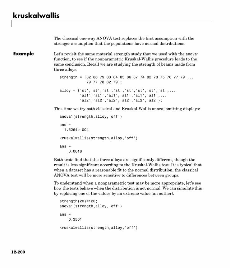
kruskalwallis
The classical one-way ANOVA test replaces the first assumption with the stronger assumption that the populations have normal distributions.
Example Let’s revisit the same material strength study that we used with the anova1 function, to see if the nonparametric Kruskal-Wallis procedure leads to the same conclusion. Recall we are studying the strength of beams made from three alloys:
strength = [82 86 79 83 84 85 86 87 74 82 78 75 76 77 79 ...79 77 78 82 79];
alloy = {'st','st','st','st','st','st','st','st',...'al1','al1','al1','al1','al1','al1',...'al2','al2','al2','al2','al2','al2'};
This time we try both classical and Kruskal-Wallis anova, omitting displays:
anova1(strength,alloy,'off')
ans = 1.5264e-004
kruskalwallis(strength,alloy,'off')
ans = 0.0018
Both tests find that the three alloys are significantly different, though the result is less significant according to the Kruskal-Wallis test. It is typical that when a dataset has a reasonable fit to the normal distribution, the classical ANOVA test will be more sensitive to differences between groups.
To understand when a nonparametric test may be more appropriate, let’s see how the tests behave when the distribution is not normal. We can simulate this by replacing one of the values by an extreme value (an outlier).
strength(20)=120;anova1(strength,alloy,'off')
ans = 0.2501
kruskalwallis(strength,alloy,'off')
12-200

kruskalwallis
ans = 0.0060
Now the classical ANOVA test does not find a significant difference, but the nonparametric procedure does. This illustrates one of the properties of nonparametric procedures – they are often not severely affected by changes in a small portion of the data.
Reference [1] Hollander, M., and D. A. Wolfe, Nonparametric Statistical Methods, Wiley, 1973.
See Also anova1, boxplot, multcompare
12-201

ksdensity
12ksdensityPurpose Compute density estimate using a kernel smoothing method
Syntax [f,xi] = ksdensity(x)f = ksdensity(x,xi)[f,xi,u] = ksdensity(...)[...] = ksdensity(...,'param1',val1,'param2',val2,...)
Description [f,xi] = ksdensity(x) computes a probability density estimate of the sample in the vector x. f is the vector of density values evaluated at the points in xi. The estimate is based on a normal kernel function, using a window parameter ('width') that is a function of the number of points in x. The density is evaluated at 100 equally-spaced points covering the range of the data in x.
f = ksdensity(x,xi) specifies the vector xi of values where the density estimate is to be evaluated.
[f,xi,u] = ksdensity(...) also returns the width of the kernel smoothing window.
[...] = ksdensity(...,'param1',val1,'param2',val2,...) specifies parameter name/value pairs to control the density estimation. Valid parameters and their possible values are:
'kernel' The type of kernel smoother to use. Choose the value as 'normal' (default), 'box', 'triangle', or 'epanechinikov'.
Alternatively, you can specify some other function, as a function handle or as a string, e.g., @normpdf or 'normpdf'. The function must take a single argument that is an array of distances between data values and places where the density is evaluated. It must return an array of the same size containing corresponding values of the kernel function.
'npoints' The number of equally-spaced points in xi. Default is 100.
'width' The bandwidth of the kernel smoothing window. The default is optimal for estimating normal densities, but you may want to choose a smaller value to reveal features such as multiple modes.
12-202

ksdensity
Examples This example generates a mixture of two normal distributions, and plots the estimated density.
x = [randn(30,1); 5+randn(30,1)];[f,xi] = ksdensity(x); plot(xi,f);
See Also hist, @ (function handle)
References [1] Bowman, A.W. and A. Azzalini, Applied Smoothing Techniques for Data Analysis, Oxford University Press, 1997.
−6 −4 −2 0 2 4 6 8 10 120
0.02
0.04
0.06
0.08
0.1
0.12
12-203
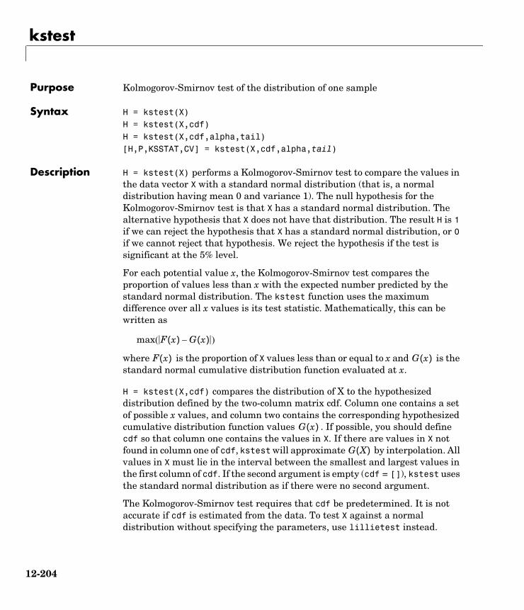
kstest
12kstestPurpose Kolmogorov-Smirnov test of the distribution of one sample
Syntax H = kstest(X)H = kstest(X,cdf)H = kstest(X,cdf,alpha,tail)[H,P,KSSTAT,CV] = kstest(X,cdf,alpha,tail)
Description H = kstest(X) performs a Kolmogorov-Smirnov test to compare the values in the data vector X with a standard normal distribution (that is, a normal distribution having mean 0 and variance 1). The null hypothesis for the Kolmogorov-Smirnov test is that X has a standard normal distribution. The alternative hypothesis that X does not have that distribution. The result H is 1 if we can reject the hypothesis that X has a standard normal distribution, or 0 if we cannot reject that hypothesis. We reject the hypothesis if the test is significant at the 5% level.
For each potential value x, the Kolmogorov-Smirnov test compares the proportion of values less than x with the expected number predicted by the standard normal distribution. The kstest function uses the maximum difference over all x values is its test statistic. Mathematically, this can be written as
where is the proportion of X values less than or equal to x and is the standard normal cumulative distribution function evaluated at x.
H = kstest(X,cdf) compares the distribution of X to the hypothesized distribution defined by the two-column matrix cdf. Column one contains a set of possible x values, and column two contains the corresponding hypothesized cumulative distribution function values . If possible, you should define cdf so that column one contains the values in X. If there are values in X not found in column one of cdf, kstest will approximate by interpolation. All values in X must lie in the interval between the smallest and largest values in the first column of cdf. If the second argument is empty (cdf = []), kstest uses the standard normal distribution as if there were no second argument.
The Kolmogorov-Smirnov test requires that cdf be predetermined. It is not accurate if cdf is estimated from the data. To test X against a normal distribution without specifying the parameters, use lillietest instead.
max F x( ) G x( )–( )
F x( ) G x( )
G x( )
G X( )
12-204

kstest
H = kstest(X,cdf,alpha,tail) specifies the significance level alpha and a code tail for the type of alternative hypothesis. If tail = 0 (the default), kstest performs a two-sided test with the general alternative . If tail = -1, the alternative is that . If tail = 1, the alternative is . The form of the test statistic depends on the value of tail as follows.
tail = 0:
tail = -1:
tail = 1:
[H,P,KSSTAT,CV] = kstest(X,cdf,alpha,tail) also returns the observed p-value P, the observed Kolmogorov-Smirnov statistic KSSTAT, and the cutoff value CV for determining if KSSTAT is significant. If the return value of CV is NaN, then kstest determined the significance calculating a p-value according to an asymptotic formula rather than by comparing KSSTAT to a critical value.
Examples Example 1. Let’s generate some evenly spaced numbers and perform a Kolmogorov-Smirnov test to see how well they fit to a normal distribution:
x = -2:1:4x = -2 -1 0 1 2 3 4
[h,p,k,c] = kstest(x,[],0.05,0)
h = 0p = 0.13632k = 0.41277c = 0.48342
We cannot reject the null hypothesis that the values come from a standard normal distribution. Although intuitively it seems that these evenly-spaced integers could not follow a normal distribution, this example illustrates the difficulty in testing normality in small samples.
F G≠F G< F G>
max F x( ) G x( )–( )
max G x( ) F x( )–( )
max F x( ) G x( )–( )
12-205

kstest
To understand the test, it is helpful to generate an empirical cumulative distribution plot and overlay the theoretical normal distribution.
xx = -3:.1:5;cdfplot(x)hold onplot(xx,normcdf(xx),'r--')
The Kolmogorov-Smirnov test statistic is the maximum difference between these curves. It appears that this maximum of 0.41277 occurs as we approach x = 1.0 from below. We can see that the empirical curve has the value 3/7 here, and we can easily verify that the difference between the curves is 0.41277.
normcdf(1) - 3/7ans = 0.41277
We can also perform a one-sided test. By setting tail = -1 we indicate that our alternative is , so the test statistic counts only points where this inequality is true.
[h,p,k] = kstest(x, [], .05, -1)
h = 0
p =
−3 −2 −1 0 1 2 3 4 50
0.1
0.2
0.3
0.4
0.5
0.6
0.7
0.8
0.9
1
x
F(x
)
Empirical CDF
F G<
12-206

kstest
0.068181
k = 0.41277
The test statistic is the same as before because in fact at x = 1.0. However, the p-value is smaller for the one-sided test. If we carry out the other one-sided test, we see that the test statistic changes, and is the difference between the two curves near x = -1.0.
[h,p,k] = kstest(x,[],0.05,1)
h = 0
p = 0.77533
k = 0.12706
2/7 - normcdf(-1)
ans = 0.12706
Example 2. Now let’s generate random numbers from a Weibull distribution, and test against that Weibull distribution and an exponential distribution.
x = weibrnd(1, 2, 100, 1);kstest(x, [x weibcdf(x, 1, 2)])
ans = 0
kstest(x, [x expcdf(x, 1)])
ans = 1
See Also kstest2, lillietest
F G<
12-207
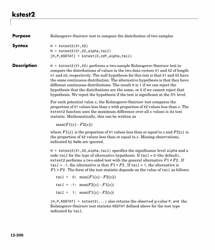
kstest2
12kstest2Purpose Kolmogorov-Smirnov test to compare the distribution of two samples
Syntax H = kstest2(X1,X2)H = kstest2(X1,X2,alpha,tail)[H,P,KSSTAT] = kstest(X,cdf,alpha,tail)
Description H = kstest2(X1,X2) performs a two-sample Kolmogorov-Smirnov test to compare the distributions of values in the two data vectors X1 and X2 of length n1 and n2, respectively. The null hypothesis for this test is that X1 and X2 have the same continuous distribution. The alternative hypothesis is that they have different continuous distributions. The result H is 1 if we can reject the hypothesis that the distributions are the same, or 0 if we cannot reject that hypothesis. We reject the hypothesis if the test is significant at the 5% level.
For each potential value x, the Kolmogorov-Smirnov test compares the proportion of X1 values less than x with proportion of X2 values less than x. The kstest2 function uses the maximum difference over all x values is its test statistic. Mathematically, this can be written as
where is the proportion of X1 values less than or equal to x and is the proportion of X2 values less than or equal to x. Missing observations, indicated by NaNs are ignored.
H = kstest2(X1,X2,alpha,tail) specifies the significance level alpha and a code tail for the type of alternative hypothesis. If tail = 0 (the default), kstest2 performs a two-sided test with the general alternative . If tail = -1, the alternative is that . If tail = 1, the alternative is
. The form of the test statistic depends on the value of tail as follows:
tail = 0:
tail = -1:
tail = 1:
[H,P,KSSTAT] = kstest2(...) also returns the observed p-value P, and the Kolmogorov-Smirnov test statistic KSSTAT defined above for the test type indicated by tail.
max F1 x( ) F2 x( )–( )
F1 x( ) F2 x( )
F1 F2≠F1 F2<
F1 F2>
max F1 x( ) F2 x( )–( )
max F2 x( ) F1 x( )–( )
max F1 x( ) F2 x( )–( )
12-208

kstest2
The asymptotic p-value becomes very accurate for large sample sizes, and is believed to be reasonably accurate for sample sizes n1 and n2 such that (n1*n2)/(n1 + n2) >= 4.
Examples Let’s compare the distributions of a small evenly-spaced sample and a larger normal sample:
x = -1:1:5y = randn(20,1);[h,p,k] = kstest2(x,y)
h = 1p = 0.0403k = 0.5714
The difference between their distributions is significant at the 5% level (p = 4%). To visualize the difference, we can overlay plots of the two empirical cumulative distribution functions. The Kolmogorov-Smirnov statistic is the maximum difference between these functions. After changing the color and line style of one of the two curves, we can see that the maximum difference appears to be near x = 1.9. We can also verify that the difference equals the k value that kstest2 reports:
cdfplot(x)hold oncdfplot(y)h = findobj(gca,'type','line');set(h(1),'linestyle',':','color','r')
1 - 3/7
ans = 0.5714
12-209
kstest2
See Also kstest, lillietest
−2 −1 0 1 2 3 4 50
0.1
0.2
0.3
0.4
0.5
0.6
0.7
0.8
0.9
1
x
F(x
)
Empirical CDF
12-210

kurtosis
12kurtosisPurpose Sample kurtosis
Syntax k = kurtosis(X)k = kurtosis(X,flag)
Description k = kurtosis(X) returns the sample kurtosis of X. For vectors, kurtosis(x) is the kurtosis of the elements in the vector x. For matrices kurtosis(X) returns the sample kurtosis for each column of X.
Kurtosis is a measure of how outlier-prone a distribution is. The kurtosis of the normal distribution is 3. Distributions that are more outlier-prone than the normal distribution have kurtosis greater than 3; distributions that are less outlier-prone have kurtosis less than 3.
The kurtosis of a distribution is defined as
where is the mean of x, is the standard deviation of x, and E(t) represents the expected value of the quantity t.
Note Some definitions of kurtosis subtract 3 from the computed value, so that the normal distribution has kurtosis of 0. The kurtosis function does not use this convention.
k = kurtosis(X,flag) specifies whether to correct for bias (flag = 0) or not (flag = 1, the default). When X represents a sample from a population, the kurtosis of X is biased, that is, it will tend to differ from the population kurtosis by a systematic amount that depends on the size of the sample. You can set flag = 0 to correct for this systematic bias.
Example X = randn([5 4])
X = 1.1650 1.6961 -1.4462 -0.3600 0.6268 0.0591 -0.7012 -0.1356 0.0751 1.7971 1.2460 -1.3493
k E x µ–( )4
σ4------------------------=
µ σ
12-211

kurtosis
0.3516 0.2641 -0.6390 -1.2704 -0.6965 0.8717 0.5774 0.9846
k = kurtosis(X)
k = 2.1658 1.2967 1.6378 1.9589
See Also mean, moment, skewness, std, var
12-212

leverage
12leveragePurpose Leverage values for a regression
Syntax h = leverage(data)h = leverage(data,'model')
Description h = leverage(data) finds the leverage of each row (point) in the matrix data for a linear additive regression model.
h = leverage(data,'model') finds the leverage on a regression, using a specified model type, where 'model' can be one of these strings:
• 'linear' – includes constant and linear terms
• 'interaction' – includes constant, linear, and cross product terms
• 'quadratic' – includes interactions and squared terms
• 'purequadratic' – includes constant, linear, and squared terms
Leverage is a measure of the influence of a given observation on a regression due to its location in the space of the inputs.
Example One rule of thumb is to compare the leverage to 2p/n where n is the number of observations and p is the number of parameters in the model. For the Hald dataset this value is 0.7692.
load haldh = max(leverage(ingredients,'linear'))
h = 0.7004
Since 0.7004 < 0.7692, there are no high leverage points using this rule.
Algorithm [Q,R] = qr(x2fx(data,'model'));
leverage = (sum(Q'.*Q'))'
Reference [1] Goodall, C. R. (1993). Computation using the QR decomposition. Handbook in Statistics, Volume 9. Statistical Computing (C. R. Rao, ed.). Amsterdam, NL Elsevier/North-Holland.
See Also regstats
12-213

lhsdesign
12lhsdesignPurpose Generate a latin hypercube sample
Syntax X = lhsdesign(n,p)X = lhsdesign(...,'smooth','off')X = lhsdesign(...,'criterion','c')X = lhsdesign(...,'iterations',k)
Description X = lhsdesign(n,p) generates a latin hypercube sample X containing n values on each of p variables. For each column, the n values are randomly distributed with one from each interval (0,1/n), (1/n,2/n), ..., (1-1/n,1), and they are randomly permuted.
X = lhsdesign(...,'smooth','off') produces points at the midpoints of the above intervals: 0.5/n, 1.5/n, ..., 1-0.5/n. The default is 'on'.
X = lhsdesign(...,'criterion','c') iteratively generates latin hypercube samples to find the best one according to the criterion 'c', which can be:
X = lhsdesign(...,'iterations',k) iterates up to k times in an attempt to improve the design according to the specified criterion. Default is K = 5.
Latin hypercube designs are useful when you need a sample that is random but that is guaranteed to be relatively uniformly distributed over each dimension.
See Also lhsnorm, unifrnd
'none' No iteration
'maximin' Maximize minimum distance between points
'correlation' Reduce correlation
12-214

lhsnorm
12lhsnormPurpose Generate a latin hypercube sample with a normal distribution
Syntax X = lhsnorm(mu,SIGMA,n)X = lhsnorm(mu,SIGMA,n,'onoff')
Description X = lhsnorm(mu,SIGMA,n) generates a latin hypercube sample X of size n from the multivariate normal distribution with mean vector mu and covariance matrix SIGMA. X is similar to a random sample from the multivariate normal distribution, but the marginal distribution of each column is adjusted so that its sample marginal distribution is close to its theoretical normal distribution.
X = lhsnorm(mu,SIGMA,n,'onoff') controls the amount of smoothing in the sample. If 'onoff' is 'off', each column has points equally spaced on the probability scale. In other words, each column is a permutation of the values G(0.5/n), G(1.5/n), ..., G(1-0.5/n) where G is the inverse normal cumulative distribution for that column's marginal distribution. If 'onoff' is 'on' (the default), each column has points uniformly distributed on the probability scale. For example, in place of 0.5/n we use a value having a uniform distribution on the interval (0/n,1/n).
See Also lhsdesign, mvnrnd
12-215

lillietest
12lillietestPurpose Lilliefors test for goodness of fit to a normal distribution
Syntax H = lillietest(X)H = lillietest(X,alpha)[H,P,LSTAT,CV] = lillietest(X,alpha)
Description H = lillietest(X) performs the Lilliefors test on the input data vector X and returns H, the result of the hypothesis test. The result H is 1 if we can reject the hypothesis that X has a normal distribution, or 0 if we cannot reject that hypothesis. We reject the hypothesis if the test is significant at the 5% level.
The Lilliefors test evaluates the hypothesis that X has a normal distribution with unspecified mean and variance, against the alternative that X does not have a normal distribution. This test compares the empirical distribution of X with a normal distribution having the same mean and variance as X. It is similar to the Kolmogorov-Smirnov test, but it adjusts for the fact that the parameters of the normal distribution are estimated from X rather than specified in advance.
H = lillietest(X,alpha) performs the Lilliefors test at the 100*alpha% level rather than the 5% level. alpha must be between 0.01 and 0.2.
[H,P,LSTAT,CV] = lillietest(X,alpha) returns three additional outputs. P is the p-value of the test, obtained by linear interpolation in a set of table created by Lilliefors. LSTAT is the value of the test statistic. CV is the critical value for determining whether to reject the null hypothesis. If the value of LSTAT is outside the range of the Lilliefors table, P is returned as NaN but H indicates whether to reject the hypothesis.
Example Do car weights follow a normal distribution? Not exactly, because weights are always positive, and a normal distribution allows both positive and negative values. However, perhaps the normal distribution is a reasonable approximation.
load carsmall[h p l c] = lillietest(Weight);[h p l c]
ans = 1.0000 0.0232 0.1032 0.0886
12-216

lillietest
The Lilliefors test statistic of 0.10317 is larger than the cutoff value of 0.0886 for a 5% level test, so we reject the hypothesis of normality. In fact, the p-value of this test is approximately 0.02.
To visualize the distribution, we can make a histogram. This graph shows that the distribution is skewed to the right – from the peak near 2250, the frequencies drop off abruptly to the left but more gradually to the right.
hist(Weight)
Sometimes it is possible to transform a variable to make its distribution more nearly normal. A log transformation, in particular, tends to compensate for skewness to the right.
[h p l c] = lillietest(log(Weight))
ans = 0 0.13481 0.077924 0.0886
Now the p-value is approximately 0.13, so we do not reject the hypothesis.
Reference [1] Conover, W. J. (1980). Practical Nonparametric Statistics. New York, Wiley.
See Also hist, jbtest, kstest2
1500 2000 2500 3000 3500 4000 4500 50000
2
4
6
8
10
12
14
16
18
12-217

linkage
12linkagePurpose Create hierarchical cluster tree
Syntax Z = linkage(Y) Z = linkage(Y,'method')
Description Z = linkage(Y) creates a hierarchical cluster tree, using the Single Linkage algorithm. The input matrix, Y, is a distance vector of length
-by-1, where m is the number of objects in the original dataset. You can generate such a vector with the pdist function. Y can also be a more general dissimilarity matrix conforming to the output format of pdist.
Z = linkage(Y,'method') computes a hierarchical cluster tree using the algorithm specified by 'method', where 'method' can be any of the following character strings that identify ways to create the cluster hierarchy. Their definitions are explained in “Mathematical Definitions” on page 12-219.
The output, Z, is an (m-1)-by-3 matrix containing cluster tree information. The leaf nodes in the cluster hierarchy are the objects in the original dataset, numbered from 1 to m. They are the singleton clusters from which all higher clusters are built. Each newly formed cluster, corresponding to row i in Z, is assigned the index m+i, where m is the total number of initial leaves.
Columns 1 and 2, Z(i,1:2), contain the indices of the objects that were linked in pairs to form a new cluster. This new cluster is assigned the index value m+i. There are m-1 higher clusters that correspond to the interior nodes of the hierarchical cluster tree.
Column 3, Z(i,3), contains the corresponding linkage distances between the objects paired in the clusters at each row i.
'single' Shortest distance (default)
'complete' Largest distance
'average' Average distance
'centroid' Centroid distance. The output Z is meaningful only if Y contains Euclidean distances.
'ward' Incremental sum of squares
m 1–( ) m 2⁄⋅( )
12-218

linkage
For example, consider a case with 30 initial nodes. If the tenth cluster formed by the linkage function combines object 5 and object 7 and their distance is 1.5, then row 10 of Z will contain the values (5, 7, 1.5). This newly formed cluster will have the index 10+30=40. If cluster 40 shows up in a later row, that means this newly formed cluster is being combined again into some bigger cluster.
Mathematical DefinitionsThe 'method' argument is a character string that specifies the algorithm used to generate the hierarchical cluster tree information. These linkage algorithms are based on various measurements of proximity between two groups of objects. If nr is the number of objects in cluster r and ns is the number of objects in cluster s, and xri is the ith object in cluster r, the definitions of these various measurements are as follows:
• Single linkage, also called nearest neighbor, uses the smallest distance between objects in the two groups.
• Complete linkage, also called furthest neighbor, uses the largest distance between objects in the two groups.
• Average linkage uses the average distance between all pairs of objects in cluster r and cluster s.
• Centroid linkage uses the distance between the centroids of the two groups.
where
d r s,( ) min dist xri xsj,( )( ) i i … nr, ,( )∈ j 1 … ns, ,( )∈, ,=
d r s,( ) max dist xri xsj,( )( ) i 1 … nr, ,( )∈ j 1 … ns, ,( )∈, ,=
d r s,( ) 1nrns------------ dist xri xsj,( )
j 1=
ns
∑i 1=
nr
∑=
d r s,( ) d xr xs,( )=
12-219

linkage
and is defined similarly.
The centroid method can produce a cluster tree that is not monotonic. This occurs when the distance from the union of two clusters, , to a third cluster is less than the distance from either r or s to that third cluster. In this case, sections of the dendrogram change direction. This is an indication that you should use another method.
• Ward linkage uses the incremental sum of squares; that is, the increase in the total within-group sum of squares as a result of joining groups r and s. It is given by
where is the distance between cluster r and cluster s defined in the Centroid linkage. The within-group sum of squares of a cluster is defined as the sum of the squares of the distance between all objects in the cluster and the centroid of the cluster.
Example X = [3 1.7; 1 1; 2 3; 2 2.5; 1.2 1; 1.1 1.5; 3 1];Y = pdist(X);Z = linkage(Y)
Z =2.0000 5.0000 0.20003.0000 4.0000 0.50008.0000 6.0000 0.50991.0000 7.0000 0.700011.0000 9.0000 1.280612.0000 10.0000 1.3454
See Also cluster, clusterdata, cophenet, dendrogram, inconsistent, kmeans, pdist, silhouette, squareform
xr1nr------ xri
i 1=
nr
∑=
xs
r s∪
d r s,( ) nrnsdrs2 nr ns+( )⁄=
drs2
12-220

logncdf
12logncdfPurpose Lognormal cumulative distribution function
Syntax P = logncdf(X,MU,SIGMA)
Description P = logncdf(X,MU,SIGMA) computes the lognormal cdf at each of the values in X using the corresponding means in MU and standard deviations in SIGMA. Vector or matrix inputs for X, MU, and SIGMA must have the same size, which is also the size of P. A scalar input for X, MU, or SIGMA is expanded to a constant matrix with the same dimensions as the other inputs.
The lognormal cdf is
Example x = (0:0.2:10);y = logncdf(x,0,1);plot(x,y); grid;xlabel('x'); ylabel('p');
Reference [1] Evans, M., N. Hastings, and B. Peacock, Statistical Distributions, Second Edition, John Wiley and Sons, 1993. p. 102–105.
See Also cdf, logninv, lognpdf, lognrnd, lognstat
p F x µ σ,( ) 1σ 2π--------------- e
ln t( ) µ–( )– 2
2σ2--------------------------------
t----------------------------- td0
x
∫= =
0 2 4 6 8 100
0.2
0.4
0.6
0.8
1
x
p
12-221

logninv
12logninvPurpose Inverse of the lognormal cumulative distribution function (cdf)
Syntax X = logninv(P,MU,SIGMA)
Description X = logninv(P,MU,SIGMA) computes the inverse lognormal cdf with mean MU and standard deviation SIGMA, at the corresponding probabilities in P. Vector or matrix inputs for P, MU, and SIGMA must have the same size, which is also the size of X. A scalar input for P, MU, or SIGMA is expanded to a constant matrix with the same dimensions as the other inputs.
We define the lognormal inverse function in terms of the lognormal cdf as
where
Example p = (0.005:0.01:0.995);crit = logninv(p,1,0.5);plot(p,crit)xlabel('Probability');ylabel('Critical Value'); grid
Reference [1] Evans, M., N. Hastings, and B. Peacock, Statistical Distributions, Second Edition, John Wiley and Sons, 1993. p. 102–105.
x F 1– p µ σ,( ) x:F x µ σ,( ) p={ }= =
p F x µ σ,( ) 1σ 2π--------------- e
ln t( ) µ–( )– 2
2σ2--------------------------------
t----------------------------- td0
x
∫= =
0 0.2 0.4 0.6 0.8 10
2
4
6
8
10
Probability
Crit
ical
Val
ue
12-222

logninv
See Also icdf, logncdf, lognpdf, lognrnd, lognstat
12-223

lognpdf
12lognpdfPurpose Lognormal probability density function (pdf)
Syntax Y = lognpdf(X,MU,SIGMA)
Description Y = logncdf(X,MU,SIGMA) computes the lognormal cdf at each of the values in X using the corresponding means in MU and standard deviations in SIGMA. Vector or matrix inputs for X, MU, and SIGMA must have the same size, which is also the size of Y. A scalar input for X, MU, or SIGMA is expanded to a constant matrix with the same dimensions as the other inputs
The lognormal pdf is
Example x = (0:0.02:10);y = lognpdf(x,0,1);plot(x,y); grid;xlabel('x'); ylabel('p')
Reference [1] Mood, A. M., F.A. Graybill, and D.C. Boes, Introduction to the Theory of Statistics, Third Edition, McGraw-Hill 1974 p. 540–541.
See Also logncdf, logninv, lognrnd, lognstat, pdf
y f x µ σ,( ) 1xσ 2π------------------e
ln x( ) µ–( )– 2
2σ2---------------------------------
= =
0 2 4 6 8 100
0.2
0.4
0.6
0.8
x
p
12-224

lognrnd
12lognrndPurpose Random matrices from the lognormal distribution
Syntax R = lognrnd(MU,SIGMA)R = lognrnd(MU,SIGMA,m)R = lognrnd(MU,SIGMA,m,n)
Description R = lognrnd(MU,SIGMA) generates lognormal random numbers with parameters MU and SIGMA. Vector or matrix inputs for MU and SIGMA must have the same size, which is also the size of R. A scalar input for MU or SIGMA is expanded to a constant matrix with the same dimensions as the other input.
R = lognrnd(MU,SIGMA,m) generates lognormal random numbers with parameters MU and SIGMA, where m is a 1-by-2 vector that contains the row and column dimensions of R.
R = lognrnd(MU,SIGMA,m,n) generates lognormal random numbers with parameters MU and SIGMA, where scalars m and n are the row and column dimensions of R.
Example r = lognrnd(0,1,4,3)
r = 3.2058 0.4983 1.3022 1.8717 5.4529 2.3909 1.0780 1.0608 0.2355 1.4213 6.0320 0.4960
Reference [1] Evans, M., N. Hastings, and B. Peacock, Statistical Distributions, Second Edition, John Wiley and Sons, 1993. p. 102–105.
See Also random, logncdf, logninv, lognpdf, lognstat
12-225

lognstat
12lognstatPurpose Mean and variance for the lognormal distribution
Syntax [M,V] = lognstat(MU,SIGMA)
Description [M,V] = lognstat(MU,SIGMA) returns the mean and variance of the lognormal distribution with parameters MU and SIGMA. Vector or matrix inputs for MU and SIGMA must have the same size, which is also the size of M and V. A scalar input for MU or SIGMA is expanded to a constant matrix with the same dimensions as the other input.
The mean of the lognormal distribution with parameters µ and σ is
and the variance is
Example [m,v]= lognstat(0,1)
m = 1.6487
v = 4.6708
Reference [1] Mood, A. M., F.A. Graybill, and D.C. Boes, Introduction to the Theory of Statistics, Third Edition, McGraw-Hill 1974 p. 540–541.
See Also logncdf, logninv, lognrnd, lognrnd
eµ σ2
2-----+
e 2µ 2σ2+( ) e 2µ σ2+( )–
12-226

lsline
12lslinePurpose Least squares fit line(s)
Syntax lslineh = lsline
Description lsline superimposes the least squares line on each line object in the current axes (except LineStyles '-','--','.-').
h = lsline returns the handles to the line objects.
Example y = [2 3.4 5.6 8 11 12.3 13.8 16 18.8 19.9]';plot(y,'+');lsline;
See Also polyfit, polyval
0 2 4 6 8 100
5
10
15
20
12-227

mad
12madPurpose Mean absolute deviation (MAD) of a sample of data
Syntax y = mad(X)
Description y = mad(X) computes the average of the absolute differences between a set of data and the sample mean of that data. For vectors, mad(x) returns the mean absolute deviation of the elements of x. For matrices, mad(X) returns the MAD of each column of X.
The MAD is less efficient than the standard deviation as an estimate of the spread when the data is all from the normal distribution.
Multiply the MAD by 1.3 to estimate σ (the second parameter of the normal distribution).
Examples This example shows a Monte Carlo simulation of the relative efficiency of the MAD to the sample standard deviation for normal data.
x = normrnd(0,1,100,100);s = std(x);s_MAD = 1.3 ∗ mad(x);efficiency = (norm(s - 1)./norm(s_MAD - 1)).^2
efficiency =
0.5972
See Also std, range
12-228
mahal
12mahalPurpose Mahalanobis distance
Syntax d = mahal(Y,X)
Description mahal(Y,X) computes the Mahalanobis distance of each point (row) of the matrix Y from the sample in the matrix X.
The number of columns of Y must equal the number of columns in X, but the number of rows may differ. The number of rows in X must exceed the number of columns.
The Mahalanobis distance is a multivariate measure of the separation of a data set from a point in space. It is the criterion minimized in linear discriminant analysis.
Example The Mahalanobis distance of a matrix r when applied to itself is a way to find outliers.
r = mvnrnd([0 0],[1 0.9;0.9 1],100);r = [r;10 10];d = mahal(r,r);last6 = d(96:101)
last6 =
1.1036 2.2353 2.0219 0.3876 1.5571 52.7381
The last element is clearly an outlier.
See Also classify
12-229

manova1
12manova1Purpose One-way Multivariate Analysis of Variance (MANOVA)
Syntax d = manova1(X,group)d = manova1(X,group,alpha)[d,p] = manova1(...)[d,p,stats] = anova1(...)
Description d = manova1(X,group) performs a one-way Multivariate Analysis of Variance (MANOVA) for comparing the multivariate means of the columns of X, grouped by group. X is an m-by-n matrix of data values, and each row is a vector of measurements on n variables for a single observation. group is a grouping variable defined as a vector, string array, or cell array of strings. Two observations are in the same group if they have the same value in the group array. The observations in each group represent a sample from a population.
The function returns d, an estimate of the dimension of the space containing the group means. manova1 tests the null hypothesis that the means of each group are the same n-dimensional multivariate vector, and that any difference observed in the sample X is due to random chance. If d = 0, there is no evidence to reject that hypothesis. If d = 1, then you can reject the null hypothesis at the 5% level, but you cannot reject the hypothesis that the multivariate means lie on the same line. Similarly, if d = 2 the multivariate means may lie on the same plane in n-dimensional space, but not on the same line.
d = manova1(X,group,alpha) gives control of the significance level, alpha. The return value d will be the smallest dimension having p > alpha, where p is a p-value for testing whether the means lie in a space of that dimension.
[d,p] = manova1(...) also returns a p, a vector of p-values for testing whether the means lie in a space of dimension 0, 1, and so on. The largest possible dimension is either the dimension of the space, or one less than the number of groups. There is one element of p for each dimension up to, but not including, the largest.
If the ith p-value is near zero, this casts doubt on the hypothesis that the group means lie on a space of i-1 dimensions. The choice of a critical p-value to determine whether the result is judged “statistically significant” is left to the researcher and is specified by the value of the input argument alpha. It is common to declare a result significant if the p-value is less than 0.05 or 0.01.
12-230

manova1
[d,p,stats] = anova1(...) also returns stats, a structure containing additional MANOVA results. The structure contains the following fields.
The canonical variables C are linear combinations of the original variables, chosen to maximize the separation between groups. Specifically, C(:,1) is the linear combination of the X columns that has the maximum separation between groups. This means that among all possible linear combinations, it is the one with the most significant F statistic in a one-way analysis of variance.
Field Contents
W Within-groups sum of squares and cross-products matrix
B Between-groups sum of squares and cross-products matrix
T Total sum of squares and cross-products matrix
dfW Degrees of freedom for W
dfB Degrees of freedom for B
dfT Degrees of freedom for T
lambda Vector of values of Wilk’s lambda test statistic for testing whether the means have dimension 0, 1, etc.
chisq Transformation of lambda to an approximate chi-square distribution
chisqdf Degrees of freedom for chisq
eigenval Eigenvalues of
eigenvec Eigenvectors of ; these are the coefficients for the canonical variables C, and they are scaled so the within-group variance of the canonical variables is 1
canon Canonical variables C, equal to XC*eigenvec, where XC is X with columns centered by subtracting their means
mdist A vector of Mahalanobis distances from each point to the mean of its group
gmdist A matrix of Mahalanobis distances between each pair of group means
W 1– B
W 1– B
12-231

manova1
C(:,2) has the maximum separation subject to it being orthogonal to C(:,1), and so on.
You may find it useful to use the outputs from manova1 along with other functions to supplement your analysis. For example, you may want to start with a grouped scatter plot matrix of the original variables using gplotmatrix. You can use gscatter to visualize the group separation using the first two canonical variables. You can use manovacluster to graph a dendrogram showing the clusters among the group means.
AssumptionsThe MANOVA test makes the following assumptions about the data in X:
• The populations for each group are normally distributed.
• The variance-covariance matrix is the same for each population.
• All observations are mutually independent.
Example We can use manova1 to determine whether there are differences in the averages of four car characteristics, among groups defined by the country where the cars were made.
load carbig[d,p] = manova1([MPG Acceleration Weight Displacement],Origin)
d = 3
p = 0 0.0000 0.0075 0.1934
There are four dimensions in the input matrix, so the group means must lie in a four-dimensional space. manova1 shows that we cannot reject the hypothesis that the means lie in a three-dimensional subspace.
References [1] Krzanowski, W. J. Principles of Multivariate Analysis. Oxford University Press, 1988.
12-232

manova1
See Also anova1, canoncorr, gscatter, gplotmatrix, manovacluster
12-233

manovacluster
12manovaclusterPurpose Plot dendrogram showing group mean clusters after MANOVA
Syntax manovacluster(stats)manovacluster(stats,'method')H = manovacluster(stats)
Description manovacluster(stats) generates a dendrogram plot of the group means after a multivariate analysis of variance (MANOVA). stats is the output stats structure from manova1. The clusters are computed by applying the single linkage method to the matrix of Mahalanobis distances between group means.
See dendrogram for more information on the graphical output from this function. The dendrogram is most useful when the number of groups is large.
manovacluster(stats,'method') uses the specified method in place of single linkage. 'method' can be any of the following character strings that identify ways to create the cluster hierarchy. See linkage for further explanation.
H = manovacluster(stats,'method') returns a vector of handles to the lines in the figure.
Example Let’s analyze the larger car dataset to determine which countries produce cars with the most similar characteristics.
load carbigX = [MPG Acceleration Weight Displacement];[d,p,stats] = manova1(X,Origin);manovacluster(stats)
'single' Shortest distance (default)
'complete' Largest distance
'average' Average distance
'centroid' Centroid distance
'ward' Incremental sum of squares
12-234

manovacluster
See Also cluster, dendrogram, linkage, manova1
Japan Germany Italy France Sweden England USA 0
0.5
1
1.5
2
2.5
3
12-235

mean
12meanPurpose Average or mean value of vectors and matrices
Syntax m = mean(X)
Description m = mean(X) calculates the sample average
For vectors, mean(x) is the mean value of the elements in vector x. For matrices, mean(X) is a row vector containing the mean value of each column.
The mean function is part of the standard MATLAB language.
Example These commands generate five samples of 100 normal random numbers with mean, zero, and standard deviation, one. The sample averages in xbar are much less variable (0.00 ± 0.10).
x = normrnd(0,1,100,5);xbar = mean(x)
xbar =
0.0727 0.0264 0.0351 0.0424 0.0752
See Also median, std, cov, corrcoef, var
xj1n--- xij
i 1=
n
∑=
12-236

median
12medianPurpose Median value of vectors and matrices
Syntax m = median(X)
Description m = median(X) calculates the median value, which is the 50th percentile of a sample. The median is a robust estimate of the center of a sample of data, since outliers have little effect on it.
For vectors, median(x) is the median value of the elements in vector x. For matrices, median(X) is a row vector containing the median value of each column. Since median is implemented using sort, it can be costly for large matrices.
The median function is part of the standard MATLAB language.
Examples xodd = 1:5;modd = median(xodd)
modd =
3
meven = median(xeven)
meven =
2.5000
This example shows robustness of the median to outliers.
xoutlier = [x 10000];moutlier = median(xoutlier)
moutlier =
3
See Also mean, std, cov, corrcoef
12-237

mle
12mlePurpose Maximum likelihood estimation
Syntax phat = mle('dist',data)[phat,pci] = mle('dist',data)[phat,pci] = mle('dist',data,alpha)[phat,pci] = mle('dist',data,alpha,p1)
Description phat = mle('dist',data) returns the maximum likelihood estimates (MLEs) for the distribution specified in 'dist' using the sample in the vector, data. See “Overview of the Distributions” on page 2-11 for the list of available distributions.
[phat,pci] = mle('dist',data) returns the MLEs and 95% percent confidence intervals.
[phat,pci] = mle('dist',data,alpha) returns the MLEs and 100(1-alpha)% confidence intervals given the data and the specified alpha.
[phat,pci] = mle('dist',data,alpha,p1) is used for the binomial distribution only, where p1 is the number of trials.
Example rv = binornd(20,0.75)
rv = 16
[p,pci] = mle('binomial',rv,0.05,20)
p = 0.8000
pci = 0.5634 0.9427
See Also betafit, binofit, expfit, gamfit, nbinfit, normfit, normlike, poissfit, weibfit
12-238

moment
12momentPurpose Central moment of all orders
Syntax m = moment(X,order)
Description m = moment(X,order) returns the central moment of X specified by the positive integer order. For vectors, moment(x,order) returns the central moment of the specified order for the elements of x. For matrices, moment(X,order) returns central moment of the specified order for each column.
Note that the central first moment is zero, and the second central moment is the variance computed using a divisor of n rather than n-1, where n is the length of the vector x or the number of rows in the matrix X.
The central moment of order k of a distribution is defined as
where E(x) is the expected value of x.
Example X = randn([6 5])
X = 1.1650 0.0591 1.2460 -1.2704 -0.0562 0.6268 1.7971 -0.6390 0.9846 0.5135 0.0751 0.2641 0.5774 -0.0449 0.3967 0.3516 0.8717 -0.3600 -0.7989 0.7562 -0.6965 -1.4462 -0.1356 -0.7652 0.4005 1.6961 -0.7012 -1.3493 0.8617 -1.3414
m = moment(X,3)
m = -0.0282 0.0571 0.1253 0.1460 -0.4486
See Also kurtosis, mean, skewness, std, var
mn E x µ–( )k=
12-239

multcompare
12multcomparePurpose Multiple comparison test of means or other estimates
Syntax c = multcompare(stats)c = multcompare(stats,alpha)c = multcompare(stats,alpha,'displayopt')c = multcompare(stats,alpha,'displayopt','ctype')c = multcompare(stats,alpha,'displayopt','ctype','estimate')c = multcompare(stats,alpha,'displayopt','ctype','estimate',dim)[c,m] = multcompare(...)[c,m,h] = multcompare(...)
Description c = multcompare(stats) performs a multiple comparison test using the information in the stats structure, and returns a matrix c of pairwise comparison results. It also displays an interactive figure presenting a graphical representation of the test.
In a one-way analysis of variance, you compare the means of several groups to test the hypothesis that they are all the same, against the general alternative that they are not all the same. Sometimes this alternative may be too general. You may need information about which pairs of means are significantly different, and which are not. A test that can provide such information is called a “multiple comparison procedure.”
When you perform a simple t-test of one group mean against another, you specify a significance level that determines the cutoff value of the t statistic. For example, you can specify the value alpha = 0.05 to insure that when there is no real difference, you will incorrectly find a significant difference no more than 5% of the time. When there are many group means, there are also many pairs to compare. If you applied an ordinary t-test in this situation, the alpha value would apply to each comparison, so the chance of incorrectly finding a significant difference would increase with the number of comparisons. Multiple comparison procedures are designed to provide an upper bound on the probability that any comparison will be incorrectly found significant.
The output c contains the results of the test in the form of a five-column matrix. Each row of the matrix represents one test, and there is one row for each pair of groups. The entries in the row indicate the means being compared, the estimated difference in means, and a confidence interval for the difference.
For example, suppose one row contains the following entries.
12-240

multcompare
2.0000 5.0000 1.9442 8.2206 14.4971
These numbers indicate that the mean of group 2 minus the mean of group 5 is estimated to be 8.2206, and a 95% confidence interval for the true mean is [1.9442, 14.4971].
In this example the confidence interval does not contain 0.0, so the difference is significant at the 0.05 level. If the confidence interval did contain 0.0, the difference would not be significant at the 0.05 level.
The multcompare function also displays a graph with each group mean represented by a symbol and an interval around the symbol. Two means are significantly different if their intervals are disjoint, and are not significantly different if their intervals overlap. You can use the mouse to select any group, and the graph will highlight any other groups that are significantly different from it.
c = multcompare(stats,alpha) determines the confidence levels of the intervals in the c matrix and in the figure. The confidence level is 100*(1-alpha)%. The default value of alpha is 0.05.
c = multcompare(stats,alpha,'displayopt') enables the graph display when 'displayopt' is 'on' (default) and suppresses the display when 'displayopt' is 'off'.
12-241

multcompare
c = multcompare(stats,alpha,'displayopt','ctype') specifies the critical value to use for the multiple comparison, which can be any of the following.
ctype Meaning
'hsd', or 'tukey-kramer'
Use Tukey's honestly significant difference criterion. This is the default, and it is based on the Studentized range distribution. It is optimal for balanced one-way ANOVA and similar procedures with equal sample sizes. It has been proven to be conservative for one-way ANOVA with different sample sizes. According to the unproven Tukey-Kramer conjecture, it is also accurate for problems where the quantities being compared are correlated, as in analysis of covariance with unbalanced covariate values.
'lsd' Use Tukey's least significant difference procedure. This procedure is a simple t-test. It is reasonable if the preliminary test (say, the one-way ANOVA F statistic) shows a significant difference. If it is used unconditionally, it provides no protection against multiple comparisons.
'bonferroni' Use critical values from the t distribution, after a Bonferroni adjustment to compensate for multiple comparisons. This procedure is conservative, but usually less so than the Scheffé procedure.
'dunn-sidak' Use critical values from the t distribution, after an adjustment for multiple comparisons that was proposed by Dunn and proved accurate by Šidák. This procedure is similar to, but less conservative than, the Bonferroni procedure.
'scheffe' Use critical values from Scheffé’s S procedure, derived from the F distribution. This procedure provides a simultaneous confidence level for comparisons of all linear combinations of the means, and it is conservative for comparisons of simple differences of pairs.
12-242

multcompare
c = multcompare(stats,alpha,'displayopt','ctype','estimate')specifies the estimate to be compared. The allowable values of estimate depend on the function that was the source of the stats structure, according to the following table.
c = multcompare(stats,alpha,'displayopt','ctype','estimate',dim)specifies the population marginal means to be compared. This argument is used only if the input stats structure was created by the anovan function. For n-way ANOVA with n factors, you can specify dim as a scalar or a vector of integers between 1 and n. The default value is 1.
For example, if dim = 1, the estimates that are compared are the means for each value of the first grouping variable, adjusted by removing effects of the other grouping variables as if the design were balanced. If dim = [1 3], population marginal means are computed for each combination of the first and third grouping variables, removing effects of the second grouping variable. If you fit a singular model, some cell means may not be estimable and any population marginal means that depend on those cell means will have the value NaN.
Source Allowable Values of Estimate
'anova1' Ignored. Always compare the group means.
'anova2' Either 'column' (the default) or 'row' to compare column or row means.
'anovan' Ignored. Always compare the population marginal means as specified by the dim argument.
'aoctool' Either 'slope', 'intercept', or 'pmm' to compare slopes, intercepts, or population marginal means. If the analysis of covariance model did not include separate slopes, then 'slope' is not allowed. If it did not include separate intercepts, then no comparisons are possible.
'friedman' Ignored. Always compare average column ranks.
'kruskalwallis' Ignored. Always compare average group ranks.
12-243
multcompare
Population marginal means are described by Milliken and Johnson (1992) and by Searle, Speed, and Milliken (1980). The idea behind population marginal means is to remove any effect of an unbalanced design by fixing the values of the factors specified by dim, and averaging out the effects of other factors as if each factor combination occurred the same number of times. The definition of population marginal means does not depend on the number of observations at each factor combination. For designed experiments where the number of observations at each factor combination has no meaning, population marginal means can be easier to interpret than simple means ignoring other factors. For surveys and other studies where the number of observations at each combination does have meaning, population marginal means may be harder to interpret.
[c,m] = multcompare(...) returns an additional matrix m. The first column of m contains the estimated values of the means (or whatever statistics are being compared) for each group, and the second column contains their standard errors.
[c,m,h] = multcompare(...) returns a handle h to the comparison graph. Note that the title of this graph contains instructions for interacting with the graph, and the x-axis label contains information about which means are significantly different from the selected mean. If you plan to use this graph for presentation, you may want to omit the title and the x-axis label. You can remove them using interactive features of the graph window, or you can use the following commands.
title('')xlabel('')
Example Let’s revisit the anova1 example testing the material strength in structural beams. From the anova1 output we found significant evidence that the three types of beams are not equivalent in strength. Now we can determine where those differences lie. First we create the data arrays and we perform one-way ANOVA.
strength = [82 86 79 83 84 85 86 87 74 82 78 75 76 77 79 ... 79 77 78 82 79];alloy = {'st','st','st','st','st','st','st','st',... 'al1','al1','al1','al1','al1','al1',... 'al2','al2','al2','al2','al2','al2'};
12-244

multcompare
[p,a,s] = anova1(strength,alloy);
Among the outputs is a structure that we can use as input to multcompare.
multcompare(s)
ans = 1.0000 2.0000 3.6064 7.0000 10.3936 1.0000 3.0000 1.6064 5.0000 8.3936 2.0000 3.0000 -5.6280 -2.0000 1.6280
The third row of the output matrix shows that the differences in strength between the two alloys is not significant. A 95% confidence interval for the difference is [-5.6, 1.6], so we cannot reject the hypothesis that the true difference is zero.
The first two rows show that both comparisons involving the first group (steel) have confidence intervals that do not include zero. In other words, those differences are significant. The graph shows the same information.
See Also anova1, anova2, anovan, aoctool, friedman, kruskalwallis
References [1] Hochberg, Y., and A. C. Tamhane, Multiple Comparison Procedures, 1987, Wiley.
74 76 78 80 82 84 86
al2
al1
st
Click on the group you want to test
2 groups have slopes significantly different from st
12-245

multcompare
[2] Milliken, G. A., and D. E. Johnson, Analysis of Messy Data, Volume 1: Designed Experiments, 1992, Chapman & Hall.
[3] Searle, S. R., F. M. Speed, and G. A. Milliken, “Population marginal means in the linear model: an alternative to least squares means,” American Statistician, 1980, pp. 216-221.
12-246

mvnpdf
12mvnpdfPurpose Multivariate normal probability density function (pdf)
Syntax y = mvnpdf(X)y = mvnpdf(X,MU)y = mvnpdf(X,MU,SIGMA)
Description y = mvnpdf(X) returns the n-by-1 vector y, containing the probability density of the multivariate normal distribution with zero mean and identity covariance matrix, evaluated at each row of the n-by-d matrix X. Rows of X correspond to observations and columns correspond to variables or coordinates.
y = mvnpdf(X,MU) returns the density of the multivariate normal distribution with mean MU and identity covariance matrix, evaluated at each row of X. MU is a 1-by-d vector, or an n-by-d matrix. If MU is a matrix, the density is evaluated for each row of X with the corresponding row of MU. MU can also be a scalar value, which mvnpdf replicates to match the size of X.
y = mvnpdf(X,MU,SIGMA) returns the density of the multivariate normal distribution with mean MU and covariance SIGMA, evaluated at each row of X. SIGMA is a d-by-d matrix, or an d-by-d-by-n array, in which case the density is evaluated for each row of X with the corresponding page of SIGMA, i.e., mvnpdf computes y(i) using X(i,:) and SIGMA(:,:,i). Specify [] for MU to use its default value when you want to specify only SIGMA.
If X is a 1-by-d vector, mvnpdf replicates it to match the leading dimension of MU or the trailing dimension of SIGMA.
Example mu = [1 -1]; Sigma = [.9 .4; .4 .3]; X = mvnrnd(mu,Sigma,10); p = mvnpdf(X,mu,Sigma);
See Also mvnrnd, normpdf
12-247

mvnrnd
12mvnrndPurpose Random matrices from the multivariate normal distribution
Syntax R = mvnrnd(MU,SIGMA)R = mvnrnd(MU,SIGMA,cases)
Description R = mvnrnd(MU,SIGMA) returns an n-by-d matrix R of random vectors chosen from the multivariate normal distribution with mean MU, and covariance SIGMA. MU is an n-by-d matrix, and mvnrnd generates each row of R using the corresponding row of MU. SIGMA is a d-by-d symmetric positive semi-definite matrix, or a d-by-d-by-n array. If SIGMA is an array, mvnrnd generates each row of R using the corresponding page of SIGMA, i.e., mvnrnd computes R(i,:) using MU(i,:) and SIGMA(:,:,i). If MU is a 1-by-d vector, mvnrnd replicates it to match the trailing dimension of SIGMA.
r = mvnrnd(MU,SIGMA,cases) returns a cases-by-d matrix R of random vectors chosen from the multivariate normal distribution with a common 1-by-d mean vector MU, and a common d-by-d covariance matrix SIGMA.
Example mu = [2 3];sigma = [1 1.5; 1.5 3];r = mvnrnd(mu,sigma,100);plot(r(:,1),r(:,2),'+')
See Also lhsnorm, mvnpdf, normrnd
-1 0 1 2 3 4 5-2
0
2
4
6
8
12-248

mvtrnd
12mvtrndPurpose Random matrices from the multivariate t distribution
Syntax r = mvtrnd(C,df,cases)
Description r = mvtrnd(C,df,cases) returns a matrix of random numbers chosen from the multivariate t distribution, where C is a correlation matrix. df is the degrees of freedom and is either a scalar or is a vector with cases elements. If p is the number of columns in C, then the output r has cases rows and p columns.
Let t represent a row of r. Then the distribution of t is that of a vector having a multivariate normal distribution with mean 0, variance 1, and covariance matrix C, divided by an independent chi-square random value having df degrees of freedom. The rows of r are independent.
C must be a square, symmetric and positive definite matrix. If its diagonal elements are not all 1 (that is, if C is a covariance matrix rather than a correlation matrix), mvtrnd computes the equivalent correlation matrix before generating the random numbers.
Example sigma = [1 0.8;0.8 1];r = mvtrnd(sigma,3,100);plot(r(:,1),r(:,2),'+')
See Also mvnrnd, trnd
−4 −2 0 2 4 6 8 10 12−4
−2
0
2
4
6
8
10
12-249

nanmax
12nanmaxPurpose Maximum ignoring NaNs
Syntax m = nanmax(a)[m,ndx] = nanmax(a)m = nanmax(a,b)
Description m = nanmax(a) returns the maximum with NaNs treated as missing. For vectors, nanmax(a) is the largest non-NaN element in a. For matrices, nanmax(A) is a row vector containing the maximum non-NaN element from each column.
[m,ndx] = nanmax(a) also returns the indices of the maximum values in vector ndx.
m = nanmax(a,b) returns the larger of a or b, which must match in size.
Example m = magic(3);m([1 6 8]) = [NaN NaN NaN]
m =
NaN 1 6 3 5 NaN 4 NaN 2
[nmax,maxidx] = nanmax(m)
nmax =
4 5 6
maxidx =
3 2 1
See Also nanmin, nanmean, nanmedian, nanstd, nansum
12-250

nanmean
12nanmeanPurpose Mean ignoring NaNs
Syntax y = nanmean(X)
Description y = nanmean(X) is the average computed by treating NaNs as missing values.
For vectors, nanmean(x) is the mean of the non-NaN elements of x. For matrices, nanmean(X) is a row vector containing the mean of the non-NaN elements in each column.
Example m = magic(3);m([1 6 8]) = [NaN NaN NaN]
m =
NaN 1 6 3 5 NaN 4 NaN 2
nmean = nanmean(m)
nmean =
3.5000 3.0000 4.0000
See Also nanmin, nanmax, nanmedian, nanstd, nansum
12-251

nanmedian
12nanmedianPurpose Median ignoring NaNs
Syntax y = nanmedian(X)
Description y = nanmedian(X) is the median computed by treating NaNs as missing values.
For vectors, nanmedian(x) is the median of the non-NaN elements of x. For matrices, nanmedian(X) is a row vector containing the median of the non-NaN elements in each column of X.
Example m = magic(4);m([1 6 9 11]) = [NaN NaN NaN NaN]
m =
NaN 2 NaN 13 5 NaN 10 8 9 7 NaN 12 4 14 15 1
nmedian = nanmedian(m)
nmedian =
5.0000 7.0000 12.5000 10.0000
See Also nanmin, nanmax, nanmean, nanstd, nansum
12-252

nanmin
12nanminPurpose Minimum ignoring NaNs
Syntax m = nanmin(a)[m,ndx] = nanmin(a)m = nanmin(a,b)
Description m = nanmin(a) is the minimum computed by treating NaNs as missing values. For vectors, nanmin(a) is the smallest non-NaN element in a. For matrices, nanmin(A) is a row vector containing the minimum non-NaN element from each column.
[m,ndx] = nanmin(a) also returns the indices of the minimum values in vector ndx.
m = nanmin(a,b) returns the smaller of a or b, which must match in size.
Example m = magic(3);m([1 6 8]) = [NaN NaN NaN]
m =
NaN 1 6 3 5 NaN 4 NaN 2
[nmin,minidx] = nanmin(m)
nmin =
3 1 2
minidx =
2 1 3
See Also nanmax, nanmean, nanmedian, nanstd, nansum
12-253

nanstd
12nanstdPurpose Standard deviation ignoring NaNs
Syntax y = nanstd(X)
Description y = nanstd(X) is the standard deviation computed by treating NaNs as missing values.
For vectors, nanstd(x) is the standard deviation of the non-NaN elements of x. For matrices, nanstd(X) is a row vector containing the standard deviations of the non-NaN elements in each column of X.
Example m = magic(3);m([1 6 8]) = [NaN NaN NaN]
m =
NaN 1 6 3 5 NaN 4 NaN 2
nstd = nanstd(m)
nstd =
0.7071 2.8284 2.8284
See Also nanmax, nanmin, nanmean, nanmedian, nansum
12-254

nansum
12nansumPurpose Sum ignoring NaNs
Syntax y = nansum(X)
Description y = nansum(X) is the sum computed by treating NaNs as missing values.
For vectors, nansum(x) is the sum of the non-NaN elements of x. For matrices, nansum(X) is a row vector containing the sum of the non-NaN elements in each column of X.
Example m = magic(3);m([1 6 8]) = [NaN NaN NaN]
m =
NaN 1 6 3 5 NaN 4 NaN 2
nsum = nansum(m)
nsum =
7 6 8
See Also nanmax, nanmin, nanmean, nanmedian, nanstd
12-255

nbincdf
12nbincdfPurpose Negative binomial cumulative distribution function (cdf)
Syntax Y = nbincdf(X,R,P)
Description Y = nbincdf(X,R,P) computes the negative binomial cdf at each of the values in X using the corresponding parameters in R and P. Vector or matrix inputs for X, R, and P must have the same size, which is also the size of Y. A scalar input for X, R, or P is expanded to a constant matrix with the same dimensions as the other inputs.
The negative binomial cdf is
The simplest motivation for the negative binomial is the case of successive random trials, each having a constant probability P of success. The number of extra trials you must perform in order to observe a given number R of successes has a negative binomial distribution. However, consistent with a more general interpretation of the negative binomial, nbincdf allows R to be any positive value, including nonintegers. When R is noninteger, the binomial coefficient in the definition of the cdf is replaced by the equivalent expression
Example x = (0:15);p = nbincdf(x,3,0.5);stairs(x,p)
y F x r p,( ) r i 1–+i
i 0=
x
∑ prqiI 0 1 …, ,( ) i( )= =
Γ r i+( )Γ r( )Γ i 1+( )--------------------------------
12-256

nbincdf
See Also cdf, nbinfit, nbininv, nbinpdf, nbinrnd, nbinstat
0 5 10 150
0.2
0.4
0.6
0.8
1
12-257

nbinfit
12nbinfitPurpose Parameter estimates and confidence intervals for negative binomial data
Syntax parmhat = nbinfit(x)[parmhat,parmci] = nbinfit(x,alpha)[...] = nbinfit(...,options)
Description parmhat = nbinfit(x) returns the maximum likelihood estimates (MLEs) of the parameters of the negative binomial distribution given the data in the vector x.
[parmhat,parmci] = nbinfit(x,alpha) returns MLEs and 100*(1-alpha) percent confidence intervals. By default, alpha = 0.05, which corresponds to 95% confidence intervals.
[...] = nbinfit(...,options) specifies control parameters for the numerical optimization used to compute MLEs. Create this argument with the MATLAB optimset function. The default is optimset('Display','notify').
Note The variance of a negative binomial distribution is greater than its mean. If the sample variance of the data x is less than its sample mean, nbinfit cannot compute MLEs. You should use the poissfit function instead.
See Also nbincdf, nbininv, nbinpdf, nbinrnd, nbinstat, mle, optimset
12-258
nbininv
12nbininvPurpose Inverse of the negative binomial cumulative distribution function (cdf)
Syntax X = nbininv(Y,R,P)
Description X = nbininv(Y,R,P) returns the inverse of the negative binomial cdf with parameters R and P at the corresponding probabilities in P. Since the binomial distribution is discrete, nbininv returns the least integer X such that the negative binomial cdf evaluated at X equals or exceeds Y. Vector or matrix inputs for Y, R, and P must have the same size, which is also the size of X. A scalar input for Y, R, or P is expanded to a constant matrix with the same dimensions as the other inputs.
The simplest motivation for the negative binomial is the case of successive random trials, each having a constant probability P of success. The number of extra trials you must perform in order to observe a given number R of successes has a negative binomial distribution. However, consistent with a more general interpretation of the negative binomial, nbininv allows R to be any positive value, including nonintegers.
Example How many times would you need to flip a fair coin to have a 99% probability of having observed 10 heads?
flips = nbininv(0.99,10,0.5) + 10
flips =
33
Note that you have to flip at least 10 times to get 10 heads. That is why the second term on the right side of the equals sign is a 10.
See Also icdf, nbincdf, nbinfit, nbinpdf, nbinrnd, nbinstat
12-259

nbinpdf
12nbinpdfPurpose Negative binomial probability density function
Syntax Y = nbinpdf(X,R,P)
Description Y = nbinpdf(X,R,P) returns the negative binomial pdf at each of the values in X using the corresponding parameters in R and P. Vector or matrix inputs for X, R, and P must have the same size, which is also the size of Y. A scalar input for X, R, or P is expanded to a constant matrix with the same dimensions as the other inputs. Note that the density function is zero unless the values in X are integers.
The negative binomial pdf is
The simplest motivation for the negative binomial is the case of successive random trials, each having a constant probability P of success. The number of extra trials you must perform in order to observe a given number R of successes has a negative binomial distribution. However, consistent with a more general interpretation of the negative binomial, nbinpdf allows R to be any positive value, including nonintegers. When R is noninteger, the binomial coefficient in the definition of the pdf is replaced by the equivalent expression
Example x = (0:10);y = nbinpdf(x,3,0.5);plot(x,y,'+')set(gca,'Xlim',[-0.5,10.5])
y f x r p,( ) r x 1–+x
prqxI 0 1 …, ,( ) x( )= =
Γ r x+( )Γ r( )Γ x 1+( )---------------------------------
12-260

nbinpdf
See Also nbincdf, nbinfit, nbininv, nbinrnd, nbinstat, pdf
0 2 4 6 8 100
0.05
0.1
0.15
0.2
12-261

nbinrnd
12nbinrndPurpose Random matrices from a negative binomial distribution
Syntax RND = nbinrnd(R,P)RND = nbinrnd(R,P,m)RND = nbinrnd(R,P,m,n)
Description RND = nbinrnd(R,P) is a matrix of random numbers chosen from a negative binomial distribution with parameters R and P. Vector or matrix inputs for R and P must have the same size, which is also the size of RND. A scalar input for R or P is expanded to a constant matrix with the same dimensions as the other input.
RND = nbinrnd(R,P,m) generates random numbers with parameters R and P, where m is a 1-by-2 vector that contains the row and column dimensions of RND.
RND = nbinrnd(R,P,m,n) generates random numbers with parameters R and P, where scalars m and n are the row and column dimensions of RND.
The simplest motivation for the negative binomial is the case of successive random trials, each having a constant probability P of success. The number of extra trials you must perform in order to observe a given number R of successes has a negative binomial distribution. However, consistent with a more general interpretation of the negative binomial, nbinrnd allows R to be any positive value, including nonintegers.
Example Suppose you want to simulate a process that has a defect probability of 0.01. How many units might Quality Assurance inspect before finding three defective items?
r = nbinrnd(3,0.01,1,6) + 3
r =
496 142 420 396 851 178
See Also nbincdf, nbinfit, nbininv, nbinpdf, nbinstat
12-262
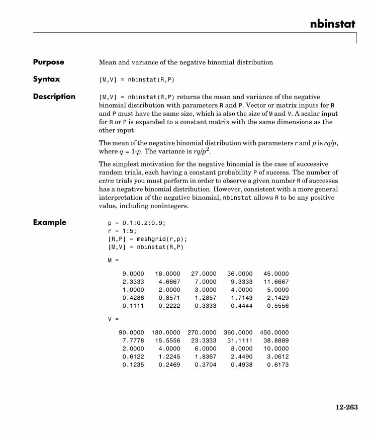
nbinstat
12nbinstatPurpose Mean and variance of the negative binomial distribution
Syntax [M,V] = nbinstat(R,P)
Description [M,V] = nbinstat(R,P) returns the mean and variance of the negative binomial distribution with parameters R and P. Vector or matrix inputs for R and P must have the same size, which is also the size of M and V. A scalar input for R or P is expanded to a constant matrix with the same dimensions as the other input.
The mean of the negative binomial distribution with parameters r and p is rq/p, where q = 1-p. The variance is rq/p2.
The simplest motivation for the negative binomial is the case of successive random trials, each having a constant probability P of success. The number of extra trials you must perform in order to observe a given number R of successes has a negative binomial distribution. However, consistent with a more general interpretation of the negative binomial, nbinstat allows R to be any positive value, including nonintegers.
Example p = 0.1:0.2:0.9;r = 1:5;[R,P] = meshgrid(r,p);[M,V] = nbinstat(R,P)
M =
9.0000 18.0000 27.0000 36.0000 45.0000 2.3333 4.6667 7.0000 9.3333 11.6667 1.0000 2.0000 3.0000 4.0000 5.0000 0.4286 0.8571 1.2857 1.7143 2.1429 0.1111 0.2222 0.3333 0.4444 0.5556
V =
90.0000 180.0000 270.0000 360.0000 450.0000 7.7778 15.5556 23.3333 31.1111 38.8889 2.0000 4.0000 6.0000 8.0000 10.0000 0.6122 1.2245 1.8367 2.4490 3.0612 0.1235 0.2469 0.3704 0.4938 0.6173
12-263

nbinstat
See Also nbincdf, nbinfit, nbininv, nbinpdf, nbinrnd
12-264

ncfcdf
12ncfcdfPurpose Noncentral F cumulative distribution function (cdf)
Syntax P = ncfcdf(X,NU1,NU2,DELTA)
Description P = ncfcdf(X,NU1,NU2,DELTA) computes the noncentral F cdf at each of the values in X using the corresponding numerator degrees of freedom in NU1, denominator degrees of freedom in NU2, and positive noncentrality parameters in DELTA. Vector or matrix inputs for X, NU1, NU2, and DELTA must have the same size, which is also the size of P. A scalar input for X, NU1, NU2, or DELTA is expanded to a constant matrix with the same dimensions as the other inputs.
The noncentral F cdf is
where I(x|a,b) is the incomplete beta function with parameters a and b.
Example Compare the noncentral F cdf with δ = 10 to the F cdf with the same number of numerator and denominator degrees of freedom (5 and 20 respectively).
x = (0.01:0.1:10.01)';p1 = ncfcdf(x,5,20,10);p = fcdf(x,5,20);plot(x,p,'--',x,p1,'-')
F x ν1 ν2 δ, ,( )
12---δ j
j!--------------e
δ2---–
Iν1 x⋅
ν2 ν+ 1 x⋅-------------------------
ν12------ j+
ν22------,
j 0=
∞
∑=
0 2 4 6 8 10 120
0.2
0.4
0.6
0.8
1
12-265

ncfcdf
References [1] Johnson, N., and S. Kotz, Distributions in Statistics: Continuous Univariate Distributions-2, John Wiley and Sons, 1970. pp. 189–200.
See Also cdf, ncfpdf, ncfinv, ncfrnd, ncfstat
12-266

ncfinv
12ncfinvPurpose Inverse of the noncentral F cumulative distribution function (cdf)
Syntax X = ncfinv(P,NU1,NU2,DELTA)
Description X = ncfinv(P,NU1,NU2,DELTA) returns the inverse of the noncentral F cdf with numerator degrees of freedom NU1, denominator degrees of freedom NU2, and positive noncentrality parameter DELTA for the corresponding probabilities in P. Vector or matrix inputs for P, NU1, NU2, and DELTA must have the same size, which is also the size of X. A scalar input for P, NU1, NU2, or DELTA is expanded to a constant matrix with the same dimensions as the other inputs.
Example One hypothesis test for comparing two sample variances is to take their ratio and compare it to an F distribution. If the numerator and denominator degrees of freedom are 5 and 20 respectively, then you reject the hypothesis that the first variance is equal to the second variance if their ratio is less than that computed below.
critical = finv(0.95,5,20)
critical =
2.7109
Suppose the truth is that the first variance is twice as big as the second variance. How likely is it that you would detect this difference?
prob = 1 - ncfcdf(critical,5,20,2)
prob =
0.1297
References [1] Evans, M., N. Hastings, and B. Peacock, Statistical Distributions, Second Edition, John Wiley and Sons, 1993. p. 102–105.
[2] Johnson, N., and S. Kotz, Distributions in Statistics: Continuous Univariate Distributions-2, John Wiley and Sons, 1970. pp. 189–200.
See Also icdf, ncfcdf, ncfpdf, ncfrnd, ncfstat
12-267

ncfpdf
12ncfpdfPurpose Noncentral F probability density function
Syntax Y = ncfpdf(X,NU1,NU2,DELTA)
Description Y = ncfpdf(X,NU1,NU2,DELTA) computes the noncentral F pdf at each of the values in X using the corresponding numerator degrees of freedom in NU1, denominator degrees of freedom in NU2, and positive noncentrality parameters in DELTA. Vector or matrix inputs for X, NU1, NU2, and DELTA must have the same size, which is also the size of Y. A scalar input for P, NU1, NU2, or DELTA is expanded to a constant matrix with the same dimensions as the other inputs.
The F distribution is a special case of the noncentral F where δ = 0. As δ increases, the distribution flattens like the plot in the example.
Example Compare the noncentral F pdf with δ = 10 to the F pdf with the same number of numerator and denominator degrees of freedom (5 and 20 respectively).
x = (0.01:0.1:10.01)';p1 = ncfpdf(x,5,20,10);p = fpdf(x,5,20);plot(x,p,'--',x,p1,'-')
References [1] Johnson, N., and S. Kotz, Distributions in Statistics: Continuous Univariate Distributions-2, John Wiley and Sons, 1970. pp. 189–200.
See Also ncfcdf, ncfinv, ncfrnd, ncfstat, pdf
0 2 4 6 8 10 120
0.2
0.4
0.6
0.8
12-268

ncfrnd
12ncfrndPurpose Random matrices from the noncentral F distribution
Syntax R = ncfrnd(NU1,NU2,DELTA)R = ncfrnd(NU1,NU2,DELTA,m)R = ncfrnd(NU1,NU2,DELTA,m,n)
Description R = ncfrnd(NU1,NU2,DELTA) returns a matrix of random numbers chosen from the noncentral F distribution with parameters NU1, NU2 and DELTA. Vector or matrix inputs for NU1, NU2, and DELTA must have the same size, which is also the size of R. A scalar input for NU1, NU2, or DELTA is expanded to a constant matrix with the same dimensions as the other inputs.
R = ncfrnd(NU1,NU2,DELTA,m) returns a matrix of random numbers with parameters NU1, NU2, and DELTA, where m is a 1-by-2 vector that contains the row and column dimensions of R.
R = ncfrnd(NU1,NU2,DELTA,m,n) generates random numbers with parameters NU1, NU2, and DELTA, where scalars m and n are the row and column dimensions of R.
Example Compute six random numbers from a noncentral F distribution with 10 numerator degrees of freedom, 100 denominator degrees of freedom and a noncentrality parameter, δ, of 4.0. Compare this to the F distribution with the same degrees of freedom.
r = ncfrnd(10,100,4,1,6)
r = 2.5995 0.8824 0.8220 1.4485 1.4415 1.4864
r1 = frnd(10,100,1,6)
r1 = 0.9826 0.5911 1.0967 0.9681 2.0096 0.6598
References [1] Johnson, N., and S. Kotz, Distributions in Statistics: Continuous Univariate Distributions-2, John Wiley and Sons, 1970. pp. 189–200.
See Also ncfcdf, ncfinv, ncfpdf, ncfstat
12-269

ncfstat
12ncfstatPurpose Mean and variance of the noncentral F distribution
Syntax [M,V] = ncfstat(NU1,NU2,DELTA)
Description [M,V] = ncfstat(NU1,NU2,DELTA) returns the mean and variance of the noncentral F pdf with NU1 and NU2 degrees of freedom and noncentrality parameter DELTA. Vector or matrix inputs for NU1, NU2, and DELTA must have the same size, which is also the size of M and V. A scalar input for NU1, NU2, or DELTA is expanded to a constant matrix with the same dimensions as the other input.
The mean of the noncentral F distribution with parameters ν1, ν2, and δ is
where ν2 > 2.
The variance is
where ν2 > 4.
Example [m,v]= ncfstat(10,100,4)
m = 1.4286
v = 3.9200
References [1] Evans, M., N. Hastings, and B. Peacock, Statistical Distributions, Second Edition, John Wiley and Sons, 1993. p. 73–74.
[2] Johnson, N., and S. Kotz, Distributions in Statistics: Continuous Univariate Distributions-2, John Wiley and Sons, 1970. pp. 189–200.
See Also ncfcdf, ncfinv, ncfpdf, ncfrnd
ν2 δ ν+ 1( )ν1 ν2 2–( )--------------------------
2ν2ν1------
2 δ ν+ 1( )2 2δ ν+ 1( ) ν2 2–( )+
ν2 2–( )2 ν2 4–( )--------------------------------------------------------------------------
12-270

nctcdf
12nctcdfPurpose Noncentral T cumulative distribution function
Syntax P = nctcdf(X,NU,DELTA)
Description P = nctcdf(X,NU,DELTA) computes the noncentral T cdf at each of the values in X using the corresponding degrees of freedom in NU and noncentrality parameters in DELTA. Vector or matrix inputs for X, NU, and DELTA must have the same size, which is also the size of P. A scalar input for X, NU, or DELTA is expanded to a constant matrix with the same dimensions as the other inputs.
Example Compare the noncentral T cdf with DELTA = 1 to the T cdf with the same number of degrees of freedom (10).
x = (-5:0.1:5)';p1 = nctcdf(x,10,1);p = tcdf(x,10);plot(x,p,'--',x,p1,'-')
References [1] Evans, M., N. Hastings, and B. Peacock, Statistical Distributions, Second Edition, John Wiley and Sons, 1993. p. 147–148.
[2] Johnson, N., and S. Kotz, Distributions in Statistics: Continuous Univariate Distributions-2, John Wiley and Sons, 1970. pp. 201–219.
See Also cdf, nctcdf, nctinv, nctpdf, nctrnd, nctstat
-5 0 50
0.2
0.4
0.6
0.8
1
12-271

nctinv
12nctinvPurpose Inverse of the noncentral T cumulative distribution
Syntax X = nctinv(P,NU,DELTA)
Description X = nctinv(P,NU,DELTA) returns the inverse of the noncentral T cdf with NU degrees of freedom and noncentrality parameter DELTA for the corresponding probabilities in P. Vector or matrix inputs for P, NU, and DELTA must have the same size, which is also the size of X. A scalar input for P, NU, or DELTA is expanded to a constant matrix with the same dimensions as the other inputs.
Example x = nctinv([0.1 0.2],10,1)
x = -0.2914 0.1618
References [1] Evans, M., N. Hastings, and B. Peacock, Statistical Distributions, Second Edition, John Wiley and Sons, 1993. p. 147–148.
[2] Johnson, N., and S. Kotz, Distributions in Statistics: Continuous Univariate Distributions-2, John Wiley and Sons, 1970. pp. 201–219.
See Also icdf, nctcdf, nctpdf, nctrnd, nctstat
12-272

nctpdf
12nctpdfPurpose Noncentral T probability density function (pdf)
Syntax Y = nctpdf(X,V,DELTA)
Description Y = nctpdf(X,V,DELTA) computes the noncentral T pdf at each of the values in X using the corresponding degrees of freedom in V and noncentrality parameters in DELTA. Vector or matrix inputs for X, V, and DELTA must have the same size, which is also the size of Y. A scalar input for X, V, or DELTA is expanded to a constant matrix with the same dimensions as the other inputs.
Example Compare the noncentral T pdf with DELTA = 1 to the T pdf with the same number of degrees of freedom (10).
x = (-5:0.1:5)';p1 = nctpdf(x,10,1);p = tpdf(x,10);plot(x,p,'--',x,p1,'-')
References [1] Evans, M., N. Hastings, and B. Peacock, Statistical Distributions, Second Edition, John Wiley and Sons, 1993. p. 147–148.
[2] Johnson, N., and S. Kotz, Distributions in Statistics: Continuous Univariate Distributions-2, John Wiley and Sons, 1970. pp. 201–219.
See Also nctcdf, nctinv, nctrnd, nctstat, pdf
-5 0 50
0.1
0.2
0.3
0.4
12-273

nctrnd
12nctrndPurpose Random matrices from noncentral T distribution
Syntax R = nctrnd(V,DELTA)R = nctrnd(V,DELTA,m)R = nctrnd(V,DELTA,m,n)
Description R = nctrnd(V,DELTA) returns a matrix of random numbers chosen from the noncentral T distribution with parameters V and DELTA. Vector or matrix inputs for V and DELTA must have the same size, which is also the size of R. A scalar input for V or DELTA is expanded to a constant matrix with the same dimensions as the other input.
R = nctrnd(V,DELTA,m) returns a matrix of random numbers with parameters V and DELTA, where m is a 1-by-2 vector that contains the row and column dimensions of R.
R = nctrnd(V,DELTA,m,n) generates random numbers with parameters V and DELTA, where scalars m and n are the row and column dimensions of R.
Example nctrnd(10,1,5,1)
ans =
1.6576 1.0617 1.4491 0.2930 3.6297
References [1] Evans, M., N. Hastings, and B. Peacock, Statistical Distributions, Second Edition, John Wiley and Sons, 1993. p. 147–148.
[2] Johnson, N., and S. Kotz, Distributions in Statistics: Continuous Univariate Distributions-2, John Wiley and Sons, 1970. pp. 201–219.
See Also nctcdf, nctinv, nctpdf, nctstat
12-274

nctstat
12nctstatPurpose Mean and variance for the noncentral t distribution
Syntax [M,V] = nctstat(NU,DELTA)
Description [M,V] = nctstat(NU,DELTA) returns the mean and variance of the noncentral t pdf with NU degrees of freedom and noncentrality parameter DELTA. Vector or matrix inputs for NU and DELTA must have the same size, which is also the size of M and V. A scalar input for NU or DELTA is expanded to a constant matrix with the same dimensions as the other input.
The mean of the noncentral t distribution with parameters ν and δ is
where ν > 1.
The variance is
where ν > 2.
Example [m,v] = nctstat(10,1)
m = 1.0837
v = 1.3255
References [1] Evans, M., N. Hastings, and B. Peacock, Statistical Distributions, Second Edition, John Wiley and Sons, 1993. p. 147–148.
[2] Johnson, N., and S. Kotz, Distributions in Statistics: Continuous Univariate Distributions-2, John Wiley and Sons, 1970. pp. 201–219.
See Also nctcdf, nctinv, nctpdf, nctrnd
δ ν 2⁄( )1 2⁄ Γ ν 1–( ) 2⁄( )Γ ν 2⁄( )
-------------------------------------------------------------
νν 2–( )----------------- 1 δ2
+( ) ν2---– δ2 Γ ν 1–( ) 2⁄( )
Γ ν 2⁄( )---------------------------------
2
12-275

ncx2cdf
12ncx2cdfPurpose Noncentral chi-square cumulative distribution function (cdf)
Syntax P = ncx2cdf(X,V,DELTA)
Description P = ncx2cdf(X,V,DELTA) computes the noncentral chi-square cdf at each of the values in X using the corresponding degrees of freedom in V and positive noncentrality parameters in DELTA. Vector or matrix inputs for X, V, and DELTA must have the same size, which is also the size of P. A scalar input for X, V, or DELTA is expanded to a constant matrix with the same dimensions as the other inputs.
Some texts refer to this distribution as the generalized Rayleigh, Rayleigh-Rice, or Rice distribution.
The noncentral chi-square cdf is
Example x = (0:0.1:10)';p1 = ncx2cdf(x,4,2);p = chi2cdf(x,4);plot(x,p,'--',x,p1,'-')
References [1] Johnson, N., and S. Kotz, Distributions in Statistics: Continuous Univariate Distributions-2, John Wiley and Sons, 1970. pp. 130–148.
F x ν δ,( )
12---δ j
j!--------------e
δ2---–
Pr χν 2j+
2 x≤[ ]
j 0=
∞
∑=
0 2 4 6 8 100
0.2
0.4
0.6
0.8
1
12-276

ncx2cdf
See Also cdf, ncx2inv, ncx2pdf, ncx2rnd, ncx2stat
12-277

ncx2inv
12ncx2invPurpose Inverse of the noncentral chi-square cdf
Syntax X = ncx2inv(P,V,DELTA)
Description X = ncx2inv(P,V,DELTA) returns the inverse of the noncentral chi-square cdf with parameters V and DELTA at the corresponding probabilities in P. Vector or matrix inputs for P, V, and DELTA must have the same size, which is also the size of X. A scalar input for P, V, or DELTA is expanded to a constant matrix with the same dimensions as the other inputs.
Algorithm ncx2inv uses Newton's method to converge to the solution.
Example ncx2inv([0.01 0.05 0.1],4,2)
ans =
0.4858 1.1498 1.7066
References Evans, M., N. Hastings, and B. Peacock, Statistical Distributions, Second Edition, John Wiley and Sons, 1993. p. 50–52.
Johnson, N., and S. Kotz, Distributions in Statistics: Continuous Univariate Distributions-2, John Wiley and Sons, 1970. pp. 130–148.
See Also icdf, ncx2cdf, ncx2pdf, ncx2rnd, ncx2stat
12-278

ncx2pdf
12ncx2pdfPurpose Noncentral chi-square probability density function (pdf)
Syntax Y = ncx2pdf(X,V,DELTA)
Description Y = ncx2pdf(X,V,DELTA) computes the noncentral chi-square pdf at each of the values in X using the corresponding degrees of freedom in V and positive noncentrality parameters in DELTA. Vector or matrix inputs for X, V, and DELTA must have the same size, which is also the size of Y. A scalar input for X, V, or DELTA is expanded to a constant matrix with the same dimensions as the other inputs.
Some texts refer to this distribution as the generalized Rayleigh, Rayleigh-Rice, or Rice distribution.
Example As the noncentrality parameter δ increases, the distribution flattens as shown in the plot.
x = (0:0.1:10)';p1 = ncx2pdf(x,4,2);p = chi2pdf(x,4);plot(x,p,'--',x,p1,'-')
References [1] Johnson, N., and S. Kotz, Distributions in Statistics: Continuous Univariate Distributions-2, John Wiley and Sons, 1970. pp. 130–148.
See Also ncx2cdf, ncx2inv, ncx2rnd, ncx2stat, pdf
0 2 4 6 8 100
0.05
0.1
0.15
0.2
12-279

ncx2rnd
12ncx2rndPurpose Random matrices from the noncentral chi-square distribution
Syntax R = ncx2rnd(V,DELTA)R = ncx2rnd(V,DELTA,m)R = ncx2rnd(V,DELTA,m,n)
Description R = ncx2rnd(V,DELTA) returns a matrix of random numbers chosen from the non-central chi-square distribution with parameters V and DELTA. Vector or matrix inputs for V and DELTA must have the same size, which is also the size of R. A scalar input for V or DELTA is expanded to a constant matrix with the same dimensions as the other input.
R = ncx2rnd(V,DELTA,m) returns a matrix of random numbers with parameters V and DELTA, where m is a 1-by-2 vector that contains the row and column dimensions of R.
R = ncx2rnd(V,DELTA,m,n) generates random numbers with parameters V and DELTA, where scalars m and n are the row and column dimensions of R.
Example ncx2rnd(4,2,6,3)
ans =
6.8552 5.9650 11.2961 5.2631 4.2640 5.9495 9.1939 6.7162 3.8315 10.3100 4.4828 7.1653 2.1142 1.9826 4.6400 3.8852 5.3999 0.9282
References [1] Evans, M., N. Hastings, and B. Peacock, Statistical Distributions, Second Edition, John Wiley and Sons, 1993. p. 50–52.
[2] Johnson, N., and S. Kotz, Distributions in Statistics: Continuous Univariate Distributions-2, John Wiley and Sons, 1970. pp. 130–148.
See Also ncx2cdf, ncx2inv, ncx2pdf, ncx2stat
12-280

ncx2stat
12ncx2statPurpose Mean and variance for the noncentral chi-square distribution
Syntax [M,V] = ncx2stat(NU,DELTA)
Description [M,V] = ncx2stat(NU,DELTA) returns the mean and variance of the noncentral chi-square pdf with NU degrees of freedom and noncentrality parameter DELTA. Vector or matrix inputs for NU and DELTA must have the same size, which is also the size of M and V. A scalar input for NU or DELTA is expanded to a constant matrix with the same dimensions as the other input.
The mean of the noncentral chi-square distribution with parameters ν and δ is , and the variance is .
Example [m,v] = ncx2stat(4,2)
m = 6
v = 16
References [1] Evans, M., N. Hastings, and B. Peacock, Statistical Distributions, Second Edition, John Wiley and Sons, 1993. p. 50–52.
[2] Johnson, N., and S. Kotz, Distributions in Statistics: Continuous Univariate Distributions-2, John Wiley and Sons, 1970. pp. 130–148.
See Also ncx2cdf, ncx2inv, ncx2pdf, ncx2rnd
ν δ+ 2 ν 2δ+( )
12-281

nlinfit
12nlinfitPurpose Nonlinear least-squares data fitting by the Gauss-Newton method
Syntax beta = nlinfit(X,y,FUN,beta0)[beta,r,J] = nlinfit(X,y,FUN,beta0)
Description beta = nlinfit(X,y,FUN,beta0) estimates the coefficients of a nonlinear function using least squares. y is a vector of response (dependent variable) values. Typically, X is a design matrix of predictor (independent variable) values, with one row for each value in y. However, X can be any array that FUN can accept. FUN is a function of the form
yhat = myfun(beta,X)
where beta is a coefficient vector, and X is the design matrix. FUN returns a vector yhat of fitted y values. beta0 is a vector containing initial values for the coefficients.
[beta,r,J] = nlinfit(X,y,FUN,beta0) returns the fitted coefficients, beta, the residuals, r, and the Jacobian, J. You can use these outputs with nlpredci to produce error estimates on predictions, and with nlparci to produce error estimates on the estimated coefficients.
Note nlintool provides a GUI for performing nonlinear fits and computing confidence intervals.
Example Find the coefficients that best fit the data in reaction.mat. The chemistry behind this data set deals with reaction kinetics as a function of the partial pressure of three chemical reactants: hydrogen, n-pentane, and isopentane.
The hougen function uses the Hougen-Watson model for reaction kinetics to return the predicted values of the reaction rate.
load reactionbetafit = nlinfit(reactants,rate,@hougen,beta)
betafit =
1.2526 0.0628
12-282

nlinfit
0.0400 0.1124 1.1914
See Also hougen, nlintool, nlparci, nlpredci
12-283

nlintool
12nlintoolPurpose Fits a nonlinear equation to data and displays an interactive graph
Syntax nlintool(x,y,FUN,beta0)nlintool(x,y,FUN,beta0,alpha)nlintool(x,y,FUN,beta0,alpha,'xname','yname')
Description nlintool(x,y,FUN,beta0) is a prediction plot that provides a nonlinear curve fit to (x,y) data. It plots a 95% global confidence interval for predictions as two red curves. beta0 is a vector containing initial guesses for the parameters.
nlintool(x,y,FUN,beta0,alpha) plots a 100(1-alpha)% confidence interval for predictions.
nlintool displays a “vector” of plots, one for each column of the matrix of inputs, x. The response variable, y, is a column vector that matches the number of rows in x.
The default value for alpha is 0.05, which produces 95% confidence intervals.
nlintool(x,y,FUN,beta0,alpha,'xname','yname') labels the plot using the string matrix, 'xname' for the x variables and the string 'yname' for the y variable.
You can drag the dotted white reference line and watch the predicted values update simultaneously. Alternatively, you can get a specific prediction by typing the value for x into an editable text field. Use the pop-up menu labeled Export to move specified variables to the base workspace. You can change the type of confidence bounds using the Bounds menu.
Example See “Nonlinear Regression Models” on page 5-1.
See Also nlinfit, rstool
12-284
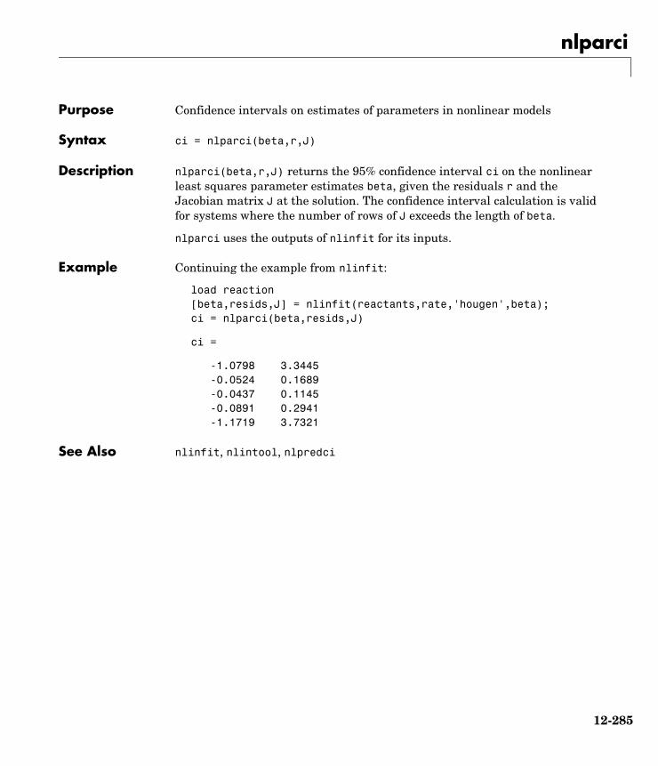
nlparci
12nlparciPurpose Confidence intervals on estimates of parameters in nonlinear models
Syntax ci = nlparci(beta,r,J)
Description nlparci(beta,r,J) returns the 95% confidence interval ci on the nonlinear least squares parameter estimates beta, given the residuals r and the Jacobian matrix J at the solution. The confidence interval calculation is valid for systems where the number of rows of J exceeds the length of beta.
nlparci uses the outputs of nlinfit for its inputs.
Example Continuing the example from nlinfit:
load reaction[beta,resids,J] = nlinfit(reactants,rate,'hougen',beta);ci = nlparci(beta,resids,J)
ci =
-1.0798 3.3445 -0.0524 0.1689 -0.0437 0.1145 -0.0891 0.2941 -1.1719 3.7321
See Also nlinfit, nlintool, nlpredci
12-285

nlpredci
12nlpredciPurpose Confidence intervals on predictions of nonlinear models
Syntax ypred = nlpredci(FUN,inputs,beta,r,J)[ypred,delta] = nlpredci(FUN,inputs,beta,r,J)ypred = nlpredci(FUN,inputs,beta,r,J,alpha,'simopt','predopt')
Description ypred = nlpredci(FUN,inputs,beta,r,J) returns the predicted responses, ypred, given the fitted parameters beta, residuals r, and the Jacobian matrix J. inputs is a matrix of values of the independent variables in the nonlinear function.
[ypred,delta] = nlpredci(FUN,inputs,beta,r,J) also returns the half-width, delta, of confidence intervals for the nonlinear least squares predictions. The confidence interval calculation is valid for systems where the length of r exceeds the length of beta and J is of full column rank. The interval [ypred-delta,ypred+delta] is a 95% non-simultaneous confidence interval for the true value of the function at the specified input values.
ypred = nlpredci(FUN,inputs,beta,r,J,alpha,'simopt','predopt')controls the type of confidence intervals. The confidence level is 100(1-alpha)%. 'simopt' can be 'on' for simultaneous intervals or 'off' (the default) for non-simultaneous intervals. 'predopt' can be 'curve' (the default) for confidence intervals for the function value at the inputs, or 'observation' for confidence intervals for a new response value.
nlpredci uses the outputs of nlinfit for its inputs.
Example Continuing the example from nlinfit, we can determine the predicted function value at [100 300 80] and the half-width of a confidence interval for it.
load reaction[beta,resids,J] = nlinfit(reactants,rate,@hougen,beta);[ypred,delta] = nlpredci(@hougen,[100 300 80],beta,resids,J)
ypred = 13
delta = 1.4277
12-286

nlpredci
See Also nlinfit, nlintool, nlparci
12-287

normcdf
12normcdfPurpose Normal cumulative distribution function (cdf)
Syntax P = normcdf(X,MU,SIGMA)
Description normcdf(X,MU,SIGMA) computes the normal cdf at each of the values in X using the corresponding parameters in MU and SIGMA. Vector or matrix inputs for X, MU, and SIGMA must all have the same size. A scalar input is expanded to a constant matrix with the same dimensions as the other inputs. The parameters in SIGMA must be positive.
The normal cdf is
The result, p, is the probability that a single observation from a normal distribution with parameters µ and σ will fall in the interval (-∞ x].
The standard normal distribution has µ = 0 and σ = 1.
Examples What is the probability that an observation from a standard normal distribution will fall on the interval [-1 1]?
p = normcdf([-1 1]);p(2) - p(1)
ans =
0.6827
More generally, about 68% of the observations from a normal distribution fall within one standard deviation, σ, of the mean, µ.
See Also cdf, normfit, norminv, normpdf, normplot, normrnd, normspec, normstat
p F x µ σ,( ) 1σ 2π--------------- e
t µ–( )– 2
2σ2---------------------
td∞–
x
∫= =
12-288

normfit
12normfitPurpose Parameter estimates and confidence intervals for normal data
Syntax [muhat,sigmahat,muci,sigmaci] = normfit(X)[muhat,sigmahat,muci,sigmaci] = normfit(X,alpha)
Description [muhat,sigmahat,muci,sigmaci] = normfit(X) returns estimates muhat and sigmahat of the normal distribution parameters µ and σ, given the matrix of data X. muci and sigmaci are 95% confidence intervals and have two rows and as many columns as matrix X. The top row is the lower bound of the confidence interval and the bottom row is the upper bound.
[muhat,sigmahat,muci,sigmaci] = normfit(X,alpha) gives estimates and 100(1-alpha)% confidence intervals. For example, alpha = 0.01 gives 99% confidence intervals.
Example In this example the data is a two-column random normal matrix. Both columns have µ = 10 and σ = 2. Note that the confidence intervals below contain the “true values.”
r = normrnd(10,2,100,2);[mu,sigma,muci,sigmaci] = normfit(r)
mu = 10.1455 10.0527
sigma = 1.9072 2.1256
muci = 9.7652 9.6288 10.5258 10.4766
sigmaci = 1.6745 1.8663 2.2155 2.4693
See Also normcdf, norminv, normlike, normpdf, normplot, normrnd, normspec, normstat, betafit, binofit, expfit, gamfit, poissfit, unifit, weibfit
12-289

norminv
12norminvPurpose Inverse of the normal cumulative distribution function (cdf)
Syntax X = norminv(P,MU,SIGMA)
Description X = norminv(P,MU,SIGMA) computes the inverse of the normal cdf with parameters MU and SIGMA at the corresponding probabilities in P. Vector or matrix inputs for P, MU, and SIGMA must all have the same size. A scalar input is expanded to a constant matrix with the same dimensions as the other inputs. The parameters in SIGMA must be positive, and the values in P must lie on the interval [0 1].
We define the normal inverse function in terms of the normal cdf as
where
The result, x, is the solution of the integral equation above where you supply the desired probability, p.
Examples Find an interval that contains 95% of the values from a standard normal distribution.
x = norminv([0.025 0.975],0,1)
x = -1.9600 1.9600
Note the interval x is not the only such interval, but it is the shortest.
xl = norminv([0.01 0.96],0,1)
xl = -2.3263 1.7507
The interval xl also contains 95% of the probability, but it is longer than x.
See Also icdf, normfit, normfit, normpdf, normplot, normrnd, normspec, normstat
x F 1– p µ σ,( ) x:F x µ σ,( ) p={ }= =
p F x µ σ,( ) 1σ 2π--------------- e
t µ–( )– 2
2σ2---------------------
td∞–
x
∫= =
12-290

normlike
12normlikePurpose Negative normal log-likelihood function
Syntax logL = normlike(params,data)[logL,avar] = normlike(params,data)
Description logL = normlike(params,data) returns the negative of the normal log-likelihood function for the parameters params(1) = mu and params(2) = sigma, given the vector data. The length of the vector logL is the length of data.
[logL,avar] = normlike(params,data) also returns the inverse of Fisher's information matrix, avar. If the input parameter values in params are the maximum likelihood estimates, the diagonal elements of avar are their asymptotic variances. avar is based on the observed Fisher's information, not the expected information.
normlike is a utility function for maximum likelihood estimation.
See Also betalike, gamlike, mle, normfit, weiblike
12-291

normpdf
12normpdfPurpose Normal probability density function (pdf)
Syntax Y = normpdf(X,MU,SIGMA)
Description normpdf(X,MU,SIGMA) computes the normal pdf at each of the values in X using the corresponding parameters in MU and SIGMA. Vector or matrix inputs for X, MU, and SIGMA must all have the same size. A scalar input is expanded to a constant matrix with the same dimensions as the other inputs. The parameters in SIGMA must be positive.
The normal pdf is
The likelihood function is the pdf viewed as a function of the parameters. Maximum likelihood estimators (MLEs) are the values of the parameters that maximize the likelihood function for a fixed value of x.
The standard normal distribution has µ = 0 and σ = 1.
If x is standard normal, then xσ + µ is also normal with mean µ and standard deviation σ. Conversely, if y is normal with mean µ and standard deviation σ, then x = (y-µ) / σ is standard normal.
Examples mu = [0:0.1:2];[y i] = max(normpdf(1.5,mu,1));MLE = mu(i)
MLE =
1.5000
See Also mvnpdf, normfit, norminv, normplot, normrnd, normspec, normstat, pdf
y f x µ σ,( ) 1σ 2π---------------e
x µ–( )– 2
2σ2----------------------
= =
12-292

normplot
12normplotPurpose Normal probability plot for graphical normality testing
Syntax normplot(X)h = normplot(X)
Description normplot(X) displays a normal probability plot of the data in X. For matrix X, normplot displays a line for each column of X.
The plot has the sample data displayed with the plot symbol '+'. Superimposed on the plot is a line joining the first and third quartiles of each column of X (a robust linear fit of the sample order statistics.) This line is extrapolated out to the ends of the sample to help evaluate the linearity of the data.
If the data does come from a normal distribution, the plot will appear linear. Other probability density functions will introduce curvature in the plot.
h = normplot(X) returns a handle to the plotted lines.
Examples Generate a normal sample and a normal probability plot of the data.
x = normrnd(0,1,50,1);h = normplot(x);
-2.5 -2 -1.5 -1 -0.5 0 0.5 1 1.5
0.01 0.02
0.05
0.10
0.25
0.50
0.75
0.90
0.95
0.98 0.99
Data
Pro
babi
lity
Normal Probability Plot
12-293

normplot
The plot is linear, indicating that you can model the sample by a normal distribution.
See Also cdfplot, hist, normfit, normfit, norminv, normpdf, normrnd, normspec, normstat
12-294

normrnd
12normrndPurpose Random numbers from the normal distribution
Syntax R = normrnd(MU,SIGMA)R = normrnd(MU,SIGMA,m)R = normrnd(MU,SIGMA,m,n)
Description R = normrnd(MU,SIGMA) generates normal random numbers with mean MU and standard deviation SIGMA. Vector or matrix inputs for MU and SIGMA must have the same size, which is also the size of R. A scalar input for MU or SIGMA is expanded to a constant matrix with the same dimensions as the other input.
R = normrnd(MU,SIGMA,m) generates normal random numbers with parameters MU and SIGMA, where m is a 1-by-2 vector that contains the row and column dimensions of R.
R = normrnd(MU,SIGMA,m,n) generates normal random numbers with parameters MU and SIGMA, where scalars m and n are the row and column dimensions of R.
Examples n1 = normrnd(1:6,1./(1:6))
n1 = 2.1650 2.3134 3.0250 4.0879 4.8607 6.2827
n2 = normrnd(0,1,[1 5])
n2 = 0.0591 1.7971 0.2641 0.8717 -1.4462
n3 = normrnd([1 2 3;4 5 6],0.1,2,3)
n3 = 0.9299 1.9361 2.9640 4.1246 5.0577 5.9864
See Also normfit, normfit, norminv, normpdf, normplot, normspec, normstat
12-295

normspec
12normspecPurpose Plot normal density between specification limits
Syntax p = normspec(specs,mu,sigma)[p,h] = normspec(specs,mu,sigma)
Description p = normspec(specs,mu,sigma) plots the normal density between a lower and upper limit defined by the two elements of the vector specs, where mu and sigma are the parameters of the plotted normal distribution.
[p,h] = normspec(specs,mu,sigma) returns the probability p of a sample falling between the lower and upper limits. h is a handle to the line objects.
If specs(1) is -Inf, there is no lower limit, and similarly if specs(2) = Inf, there is no upper limit.
Example Suppose a cereal manufacturer produces 10 ounce boxes of corn flakes. Variability in the process of filling each box with flakes causes a 1.25 ounce standard deviation in the true weight of the cereal in each box. The average box of cereal has 11.5 ounces of flakes. What percentage of boxes will have less than 10 ounces?
normspec([10 Inf],11.5,1.25)
See Also capaplot, disttool, histfit, normfit, normfit, norminv, normpdf, normplot, normrnd, normstat
6 8 10 12 14 160
0.1
0.2
0.3
0.4
Critical Value
Den
sity
Probability Between Limits is 0.8849
12-296

normstat
12normstatPurpose Mean and variance for the normal distribution
Syntax [M,V] = normstat(MU,SIGMA)
Description [M,V] = normstat(MU,SIGMA) returns the mean and variance for the normal distribution with parameters MU and SIGMA. Vector or matrix inputs for MU and SIGMA must have the same size, which is also the size of M and V. A scalar input for MU or SIGMA is expanded to a constant matrix with the same dimensions as the other input.
The mean of the normal distribution with parameters µ and σ is µ, and the variance is σ2.
Examples n = 1:5;[m,v] = normstat(n'∗ n,n'*n)[m,v] = normstat(n'*n,n'*n)
m = 1 2 3 4 5 2 4 6 8 10 3 6 9 12 15 4 8 12 16 20 5 10 15 20 25
v = 1 4 9 16 25 4 16 36 64 100 9 36 81 144 225 16 64 144 256 400 25 100 225 400 625
See Also normfit, normfit, norminv, normpdf, normplot, normrnd, normspec
12-297
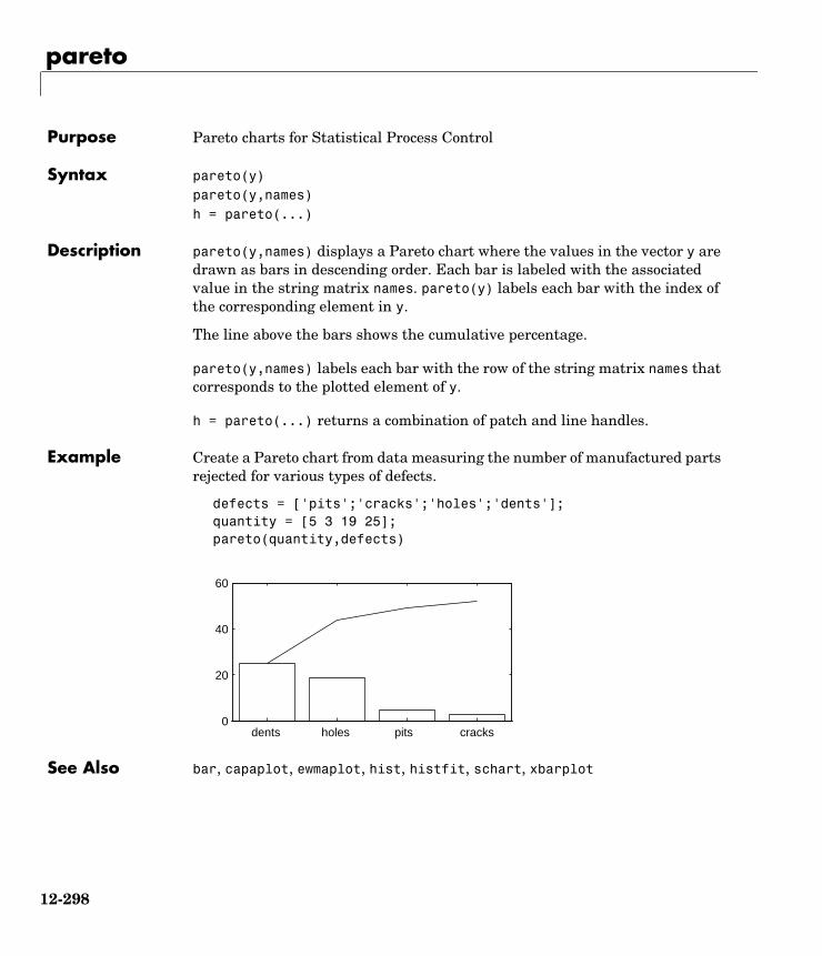
pareto
12paretoPurpose Pareto charts for Statistical Process Control
Syntax pareto(y)pareto(y,names)h = pareto(...)
Description pareto(y,names) displays a Pareto chart where the values in the vector y are drawn as bars in descending order. Each bar is labeled with the associated value in the string matrix names. pareto(y) labels each bar with the index of the corresponding element in y.
The line above the bars shows the cumulative percentage.
pareto(y,names) labels each bar with the row of the string matrix names that corresponds to the plotted element of y.
h = pareto(...) returns a combination of patch and line handles.
Example Create a Pareto chart from data measuring the number of manufactured parts rejected for various types of defects.
defects = ['pits';'cracks';'holes';'dents'];quantity = [5 3 19 25];pareto(quantity,defects)
See Also bar, capaplot, ewmaplot, hist, histfit, schart, xbarplot
dents holes pits cracks0
20
40
60
12-298

pcacov
12pcacovPurpose Principal Components Analysis (PCA) using the covariance matrix
Syntax pc = pcacov(X)[pc,latent,explained] = pcacov(X)
Description [pc,latent,explained] = pcacov(X) takes the covariance matrix X and returns the principal components in pc, the eigenvalues of the covariance matrix of X in latent, and the percentage of the total variance in the observations explained by each eigenvector in explained.
Example load haldcovx = cov(ingredients);[pc,variances,explained] = pcacov(covx)
pc =
0.0678 -0.6460 0.5673 -0.5062 0.6785 -0.0200 -0.5440 -0.4933 -0.0290 0.7553 0.4036 -0.5156 -0.7309 -0.1085 -0.4684 -0.4844
variances =
517.7969 67.4964 12.4054 0.2372
explained =
86.5974 11.2882 2.0747 0.0397
References [1] Jackson, J. E., A User's Guide to Principal Components, John Wiley and Sons, Inc. 1991. pp. 1–25.
See Also barttest, pcares, princomp
12-299

pcares
12pcaresPurpose Residuals from a Principal Components Analysis
Syntax residuals = pcares(X,ndim)
Description pcares(X,ndim) returns the residuals obtained by retaining ndim principal components of X. Note that ndim is a scalar and must be less than the number of columns in X. Use the data matrix, not the covariance matrix, with this function.
Example This example shows the drop in the residuals from the first row of the Hald data as the number of component dimensions increase from one to three.
load haldr1 = pcares(ingredients,1);r2 = pcares(ingredients,2);r3 = pcares(ingredients,3);
r11 = r1(1,:)r11 =
2.0350 2.8304 -6.8378 3.0879
r21 = r2(1,:)r21 =
-2.4037 2.6930 -1.6482 2.3425
r31 = r3(1,:)r31 =
0.2008 0.1957 0.2045 0.1921
Reference [1] Jackson, J. E., A User's Guide to Principal Components, John Wiley and Sons, Inc. 1991. pp. 1–25.
See Also barttest, pcacov, princomp
12-300

12pdfPurpose Probability density function (pdf) for a specified distribution
Syntax Y = pdf('name',X,A1,A2,A3)
Description pdf('name',X,A1,A2,A3) returns a matrix of densities, where 'name' is a string containing the name of the distribution. X is a matrix of values, and A1, A2, and A3 are matrices of distribution parameters. Depending on the distribution, some of the parameters may not be necessary.
Vector or matrix inputs for X, A1, A2, and A3 must all have the same size. A scalar input is expanded to a constant matrix with the same dimensions as the other inputs.
pdf is a utility routine allowing access to all the pdfs in the Statistics Toolbox using the name of the distribution as a parameter. See “Overview of the Distributions” on page 2-11 for the list of available distributions.
Examples p = pdf('Normal',-2:2,0,1)
p = 0.0540 0.2420 0.3989 0.2420 0.0540
p = pdf('Poisson',0:4,1:5)
p = 0.3679 0.2707 0.2240 0.1954 0.1755
See Also betapdf, binopdf, cdf, chi2pdf, exppdf, fpdf, gampdf, geopdf, hygepdf, lognpdf, nbinpdf, ncfpdf, nctpdf, ncx2pdf, normpdf, poisspdf, raylpdf, tpdf, unidpdf, unifpdf, weibpdf
12-301

pdist
12pdistPurpose Pairwise distance between observations
Syntax Y = pdist(X)Y = pdist(X,'metric')Y = pdist(X,distfun,p1,p2,...)Y = pdist(X,'minkowski',p)
Description Y = pdist(X) computes the Euclidean distance between pairs of objects in m-by-n matrix X, which is treated as m vectors of size n. For a dataset made up of m objects, there are pairs.
The output, Y, is a vector of length , containing the distance information. The distances are arranged in the order (1,2), (1,3), ..., (1,m), (2,3), ..., (2,m), ..., ..., (m-1,m). Y is also commonly known as a similarity matrix or dissimilarity matrix.
To save space and computation time, Y is formatted as a vector. However, you can convert this vector into a square matrix using the squareform function so that element i,j in the matrix, where , corresponds to the distance between objects i and j in the original dataset.
Y = pdist(X,'metric') computes the distance between objects in the data matrix, X, using the method specified by 'metric', where 'metric' can be any of the following character strings that identify ways to compute the distance.
'euclidean' Euclidean distance (default)
'seuclidean' Standardized Euclidean distance. Each coordinate in the sum of squares is inverse weighted by the sample variance of that coordinate.
'mahalanobis' Mahalanobis distance
'cityblock' City Block metric
'minkowski' Minkowski metric
'cosine' One minus the cosine of the included angle between points (treated as vectors)
'correlation' One minus the sample correlation between points (treated as sequences of values).
m 1–( ) m 2⁄⋅
m 1–( ) m 2⁄⋅
i j<
12-302

pdist
Y = pdist(X,distfun,p1,p2,...) accepts a function handle to a distance function of the form
d = distfun(XI,XJ,p1,p2,...)
taking as arguments two q-by-n matrices XI and XJ each of which contains rows of X, plus zero or more additional arguments, and returning a q-by-1 vector of distances d, whose kth element is the distance between the observations XI(k,:) and XJ(k,:). The arguments p1,p2,... are passed directly to the function distfun.
Y = pdist(X,'minkowski',p) computes the distance between objects in the data matrix, X, using the Minkowski metric. p is the exponent used in the Minkowski computation which, by default, is 2.
Mathematical Definitions of MethodsGiven an m-by-n data matrix X, which is treated as m (1-by-n) row vectors x1, x2, ..., xm, the various distances between the vector xr and xs are defined as follows:
• Euclidean distance
• Standardized Euclidean distance
where D is the diagonal matrix with diagonal elements given by , which denotes the variance of the variable Xj over the m objects.
• Mahalanobis distance
'hamming' Hamming distance, the percentage of coordinates that differ
'jaccard' One minus the Jaccard coefficient, the percentage of nonzero coordinates that differ
drs2 xr xs–( ) xr xs–( )'=
drs2 xr xs–( )D 1– xr xs–( )'=
vj2
12-303

pdist
where V is the sample covariance matrix.
• City Block metric
• Minkowski metric
Notice that for the special case of p = 1, the Minkowski metric gives the City Block metric, and for the special case of p = 2, the Minkowski metric gives the Euclidean distance.
• Cosine distance
• Correlation distance
where
and
• Hamming distance
drs2 xr xs–( )V 1– xr xs–( )′=
drs xrj xsj–j 1=
n
∑=
drs xrj xsj–p
j 1=
n
∑
1p---
=
drs 1 x– rx ′s x′rxr( )12---
x′sxs( )12---
⁄
=
drs 1xr xr–( ) xs xs–( )′
xr xr–( ) xr xr–( )′[ ]12---
xs xs–( ) xs xs–( )′[ ]12---
----------------------------------------------------------------------------------------------------------–=
xr1n--- xrj
j∑= xs
1n--- xsj
j∑=
drs # xrj xsj≠( ) n⁄( )=
12-304

pdist
• Jaccard distance
Examples X = [1 2; 1 3; 2 2; 3 1]
X = 1 2 1 3 2 2 3 1
Y = pdist(X,'mahal')Y = 2.3452 2.0000 2.3452 1.2247 2.4495 1.2247
Y = pdist(X)Y = 1.0000 1.0000 2.2361 1.4142 2.8284 1.4142
squareform(Y)
ans = 0 1.0000 1.0000 2.2361 1.0000 0 1.4142 2.8284 1.0000 1.4142 0 1.4142 2.2361 2.8284 1.4142 0
See Also cluster, clusterdata, cmdscale, cophenet, dendrogram, inconsistent, linkage, silhouette, squareform
drs
# xrj xsj≠( ) xrj 0≠( ) xsj 0≠( )∨( )∧[ ]# xrj 0≠( ) xsj 0≠( )∨[ ]
-----------------------------------------------------------------------------------------------=
12-305

perms
12permsPurpose All permutations
Syntax P = perms(v)
Description P = perms(v) where v is a row vector of length n, creates a matrix whose rows consist of all possible permutations of the n elements of v. The matrix P contains n! rows and n columns.
perms is only practical when n is less than 8 or 9.
Example perms([2 4 6])
ans =
6 4 2 4 6 2 6 2 4 2 6 4 4 2 6 2 4 6
12-306

poisscdf
12poisscdfPurpose Poisson cumulative distribution function (cdf)
Syntax P = poisscdf(X,LAMBDA)
Description poisscdf(X,LAMBDA) computes the Poisson cdf at each of the values in X using the corresponding parameters in LAMBDA. Vector or matrix inputs for X and LAMBDA must be the same size. A scalar input is expanded to a constant matrix with the same dimensions as the other input. The parameters in LAMBDA must be positive.
The Poisson cdf is
Examples For example, consider a Quality Assurance department that performs random tests of individual hard disks. Their policy is to shut down the manufacturing process if an inspector finds more than four bad sectors on a disk. What is the probability of shutting down the process if the mean number of bad sectors (λ) is two?
probability = 1 - poisscdf(4,2)
probability =
0.0527
About 5% of the time, a normally functioning manufacturing process will produce more than four flaws on a hard disk.
Suppose the average number of flaws (λ) increases to four. What is the probability of finding fewer than five flaws on a hard drive?
probability = poisscdf(4,4)
probability =
0.6288
This means that this faulty manufacturing process continues to operate after this first inspection almost 63% of the time.
p F x λ( ) e λ– λ i
i!-----
i 0=
floor x( )
∑= =
12-307

poisscdf
See Also cdf, poissfit, poissinv, poisspdf, poissrnd, poisstat
12-308

poissfit
12poissfitPurpose Parameter estimates and confidence intervals for Poisson data
Syntax lambdahat = poissfit(X)[lambdahat,lambdaci] = poissfit(X)[lambdahat,lambdaci] = poissfit(X,alpha)
Description poissfit(X) returns the maximum likelihood estimate (MLE) of the parameter of the Poisson distribution, λ, given the data X.
[lambdahat,lambdaci] = poissfit(X) also gives 95% confidence intervals in lamdaci.
[lambdahat,lambdaci] = poissfit(X,alpha) gives 100(1-alpha)% confidence intervals. For example alpha = 0.001 yields 99.9% confidence intervals.
The sample average is the MLE of λ.
Example r = poissrnd(5,10,2);[l,lci] = poissfit(r)
l =7.4000 6.3000
lci =5.8000 4.80009.1000 7.9000
See Also betafit, binofit, expfit, gamfit, poisscdf, poissinv, poisspdf, poissrnd, poisstat, unifit, weibfit
λ� 1n--- xi
i 1=
n
∑=
12-309

poissinv
12poissinvPurpose Inverse of the Poisson cumulative distribution function (cdf)
Syntax X = poissinv(P,LAMBDA)
Description poissinv(P,LAMBDA) returns the smallest value X such that the Poisson cdf evaluated at X equals or exceeds P.
Examples If the average number of defects (λ) is two, what is the 95th percentile of the number of defects?
poissinv(0.95,2)
ans =
5
What is the median number of defects?
median_defects = poissinv(0.50,2)
median_defects =
2
See Also icdf, poisscdf, poissfit, poisspdf, poissrnd, poisstat
12-310

poisspdf
12poisspdfPurpose Poisson probability density function (pdf)
Syntax Y = poisspdf(X,LAMBDA)
Description poisspdf(X,LAMBDA) computes the Poisson pdf at each of the values in X using the corresponding parameters in LAMBDA. Vector or matrix inputs for X and LAMBDA must be the same size. A scalar input is expanded to a constant matrix with the same dimensions as the other input. The parameters in LAMBDA must all be positive.
The Poisson pdf is
where x can be any nonnegative integer. The density function is zero unless x is an integer.
Examples A computer hard disk manufacturer has observed that flaws occur randomly in the manufacturing process at the average rate of two flaws in a 4 Gb hard disk and has found this rate to be acceptable. What is the probability that a disk will be manufactured with no defects?
In this problem, λ = 2 and x = 0.
p = poisspdf(0,2)
p = 0.1353
See Also pdf, poisscdf, poissfit, poissinv, poissrnd, poisstat
y f x λ( ) λx
x!-----e λ– I 0 1 …, ,( ) x( )= =
12-311

poissrnd
12poissrndPurpose Random numbers from the Poisson distribution
Syntax R = poissrnd(LAMBDA)R = poissrnd(LAMBDA,m)R = poissrnd(LAMBDA,m,n)
Description R = poissrnd(LAMBDA) generates Poisson random numbers with mean LAMBDA. The size of R is the size of LAMBDA.
R = poissrnd(LAMBDA,m) generates Poisson random numbers with mean LAMBDA, where m is a 1-by-2 vector that contains the row and column dimensions of R.
R = poissrnd(LAMBDA,m,n) generates Poisson random numbers with mean LAMBDA, where scalars m and n are the row and column dimensions of R.
Examples Generate a random sample of 10 pseudo-observations from a Poisson distribution with λ = 2.
lambda = 2;
random_sample1 = poissrnd(lambda,1,10)random_sample1 =
1 0 1 2 1 3 4 2 0 0
random_sample2 = poissrnd(lambda,[1 10])random_sample2 =
1 1 1 5 0 3 2 2 3 4
random_sample3 = poissrnd(lambda(ones(1,10)))random_sample3 =
3 2 1 1 0 0 4 0 2 0
See Also poisscdf, poissfit, poissinv, poisspdf, poisstat
12-312

poisstat
12poisstatPurpose Mean and variance for the Poisson distribution
Syntax M = poisstat(LAMBDA)[M,V] = poisstat(LAMBDA)
Description M = poisstat(LAMBDA) returns the mean of the Poisson distribution with parameter LAMBDA. The size of M is the size of LAMBDA.
[M,V] = poisstat(LAMBDA) also returns the variance V of the Poisson distribution.
For the Poisson distribution with parameter λ, both the mean and variance are equal to λ.
Examples Find the mean and variance for the Poisson distribution with λ = 2.
[m,v] = poisstat([1 2; 3 4])
m = 1 2 3 4
v = 1 2 3 4
See Also poisscdf, poissfit, poissinv, poisspdf, poissrnd
12-313

polyconf
12polyconfPurpose Polynomial evaluation and confidence interval estimation
Syntax [Y,DELTA] = polyconf(p,X,S)[Y,DELTA] = polyconf(p,X,S,alpha)
Description [Y,DELTA] = polyconf(p,X,S) uses the optional output S generated by polyfit to give 95% confidence intervals Y ± DELTA. This assumes the errors in the data input to polyfit are independent normal with constant variance.
[Y,DELTA] = polyconf(p,X,S,alpha) gives 100(1-alpha)% confidence intervals. For example, alpha = 0.1 yields 90% intervals.
If p is a vector whose elements are the coefficients of a polynomial in descending powers, such as those output from polyfit, then polyconf(p,X) is the value of the polynomial evaluated at X. If X is a matrix or vector, the polynomial is evaluated at each of the elements.
Examples This example gives predictions and 90% confidence intervals for computing time for LU factorizations of square matrices with 100 to 200 columns.
n = [100 100:20:200];for i = nA = rand(i,i);ticB = lu(A);
t(ceil((i-80)/20)) = toc;end
[p,S] = polyfit(n(2:7),t,3);[time,delta_t] = polyconf(p,n(2:7),S,0.1)
time =
0.0829 0.1476 0.2277 0.3375 0.4912 0.7032
delta_t =
0.0064 0.0057 0.0055 0.0055 0.0057 0.0064
12-314

polyfit
12polyfitPurpose Polynomial curve fitting
Syntax [p,S] = polyfit(x,y,n)
Description p = polyfit(x,y,n) finds the coefficients of a polynomial p(x) of degree n that fits the data, p(x(i)) to y(i), in a least-squares sense. The result p is a row vector of length n+1 containing the polynomial coefficients in descending powers.
[p,S] = polyfit(x,y,n) returns polynomial coefficients p and matrix S for use with polyval to produce error estimates on predictions. If the errors in the data, y, are independent normal with constant variance, polyval will produce error bounds which contain at least 50% of the predictions.
You may omit S if you are not going to pass it to polyval or polyconf for calculating error estimates.
The polyfit function is part of the standard MATLAB language.
Example [p,S] = polyfit(1:10,[1:10] + normrnd(0,1,1,10),1)
p =
1.0300 0.4561
S =
-19.6214 -2.8031 0 -1.4639 8.0000 0 2.3180 0
See Also polyval, polytool, polyconf
p x( ) p1xn p2xn 1– … pnx pn 1++ + + +=
12-315

polytool
12polytoolPurpose Interactive plot for prediction of fitted polynomials
Syntax polytool(x,y)polytool(x,y,n)polytool(x,y,n,alpha)
Description polytool(x,y) fits a line to the column vectors x and y and displays an interactive plot of the result. This plot is graphic user interface for exploring the effects of changing the polynomial degree of the fit. The plot shows the fitted curve and 95% global confidence intervals on a new predicted value for the curve. Text with current predicted value of y and its uncertainty appears to the left of the y-axis.
polytool(x,y,n) initially fits a polynomial of order n.
polytool(x,y,n,alpha) plots 100(1-alpha)% confidence intervals on the predicted values.
polytool fits by least-squares using the regression model
Evaluate the function by typing a value in the x-axis edit box or by dragging the vertical reference line on the plot. The shape of the pointer changes from an arrow to a cross hair when you are over the vertical line to indicate that the line can be dragged. The predicted value of y will update as you drag the reference line.
The argument n controls the degree of the polynomial fit. To change the degree of the polynomial, choose from the pop-up menu at the top of the figure. To change the type of confidence intervals, use the Bounds menu. To change from least squares to a robust fitting method, use the Method menu.
When you are done, press the Close button.
yi β0 β1xi β2xi2 … βnxi
n εi+ + ++ +=
εi N 0 σ2,( )∼ i∀
Cov εi εj,( ) 0= i j,∀
12-316

polyval
12polyvalPurpose Polynomial evaluation
Syntax Y = polyval(p,X)[Y,DELTA] = polyval(p,X,S)
Description Y = polyval(p,X) returns the predicted value of a polynomial given its coefficients, p, at the values in X.
[Y,DELTA] = polyval(p,X,S) uses the optional output S generated by polyfit to generate error estimates, Y ± DELTA. If the errors in the data input to polyfit are independent normal with constant variance, Y ± DELTA contains at least 50% of the predictions.
If p is a vector whose elements are the coefficients of a polynomial in descending powers, then polyval(p,X) is the value of the polynomial evaluated at X. If X is a matrix or vector, the polynomial is evaluated at each of the elements.
The polyval function is part of the standard MATLAB language.
Examples Simulate the function y = x, adding normal random errors with a standard deviation of 0.1. Then use polyfit to estimate the polynomial coefficients. Note that predicted Y values are within DELTA of the integer X in every case.
[p,S] = polyfit(1:10,(1:10) + normrnd(0,0.1,1,10),1);X = magic(3);[Y,D] = polyval(p,X,S)
Y = 8.0696 1.0486 6.0636 3.0546 5.0606 7.0666 4.0576 9.0726 2.0516
D = 0.0889 0.0951 0.0861 0.0889 0.0861 0.0870 0.0870 0.0916 0.0916
See Also polyfit, polytool, polyconf
12-317

prctile
12prctilePurpose Percentiles of a sample
Syntax Y = prctile(X,p)
Description Y = prctile(X,p) calculates a value that is greater than p percent of the values in X. The values of p must lie in the interval [0 100].
For vectors, prctile(X,p) is the pth percentile of the elements in X. For instance, if p = 50 then Y is the median of X.
For matrix X and scalar p, prctile(X,p) is a row vector containing the pth percentile of each column. If p is a vector, the ith row of Y is p(i) of X.
Examples x = (1:5)'*(1:5)
x = 1 2 3 4 5 2 4 6 8 10 3 6 9 12 15 4 8 12 16 20 5 10 15 20 25
y = prctile(x,[25 50 75])
y = 1.7500 3.5000 5.2500 7.0000 8.7500 3.0000 6.0000 9.0000 12.0000 15.0000 4.2500 8.5000 12.7500 17.0000 21.2500
12-318

princomp
12princompPurpose Principal Components Analysis (PCA)
Syntax PC = princomp(X)[PC,SCORE,latent,tsquare] = princomp(X)
Description [PC,SCORE,latent,tsquare] = princomp(X) takes a data matrix X and returns the principal components in PC, the so-called Z-scores in SCORE, the eigenvalues of the covariance matrix of X in latent, and Hotelling’s T2 statistic for each data point in tsquare.
The Z-scores are the data formed by transforming the original data into the space of the principal components. The values of the vector, latent, are the variance of the columns of SCORE. Hotelling’s T2 is a measure of the multivariate distance of each observation from the center of the data set.
Example Compute principal components for the ingredients data in the Hald dataset, and the variance accounted for by each component.
load hald;[pc,score,latent,tsquare] = princomp(ingredients);pc,latent
pc = 0.0678 -0.6460 0.5673 -0.5062 0.6785 -0.0200 -0.5440 -0.4933 -0.0290 0.7553 0.4036 -0.5156 -0.7309 -0.1085 -0.4684 -0.4844
latent =
517.7969 67.4964 12.4054 0.2372
Reference [1] Jackson, J. E., A User's Guide to Principal Components, John Wiley and Sons, Inc. 1991. pp. 1–25.
See Also barttest, canoncorr, factoran, pcacov, pcares
12-319

procrustes
12procrustesPurpose Procrustes Analysis
Syntax d = procrustes(X,Y)[d,Z] = procrustes(X,Y)[d,Z,transform] = procrustes(X,Y)
Description d = procrustes(X,Y) determines a linear transformation (translation, reflection, orthogonal rotation, and scaling) of the points in matrix Y to best conform them to the points in matrix X. The "goodness-of-fit" criterion is the sum of squared errors. procrustes returns the minimized value of this dissimilarity measure in d. d is standardized by a measure of the scale of X, given by
sum(sum((X-repmat(mean(X,1),size(X,1),1)).^2,1))
i.e., the sum of squared elements of a centered version of X. However, if X comprises repetitions of the same point, the sum of squared errors is not standardized.
X and Y must have the same number of points (rows), and procrustes matches the ith point in Y to the ith point in X. Points in Y can have smaller dimension (number of columns) than those in X. In this case, procrustes adds columns of zeros to Y as necessary.
[d,Z] = procrustes(X,Y) also returns the transformed Y values.
[d,Z,transform] = procrustes(X,Y) also returns the transformation that maps Y to Z. transform is a structure with fields:
That is, Z = transform.b * Y * transform.T + transform.c.
Examples This example creates some random points in two dimensions, then rotates, scales, translates, and adds some noise to those points. It then uses procrustes to conform Y to X, and plots the original X and Y, and the transformed Y.
c Translation component
T Orthogonal rotation and reflection component
b Scale component
12-320

procrustes
X = normrnd(0,1,[10 2]); S = [0.5 -sqrt(3)/2; sqrt(3)/2 0.5]; Y = normrnd(0.5*X*S + 2,0.05,size(X)); [d,Z,tr] = procrustes(X,Y); plot(X(:,1),X(:,2),'rx',... Y(:,1),Y(:,2),'b.',... Z(:,1),Z(:,2),'bx');
See Also cmdscale, factoran
References [1] Seber, G.A.F., Multivariate Observations, Wiley, 1984
[2] Bulfinch, T., The Age of Fable; or, Stories of Gods and Heroes, Sanborn, Carter, and Bazin, Boston, 1855.
12-321

qqplot
12qqplotPurpose Quantile-quantile plot of two samples
Syntax qqplot(X)qqplot(X,Y)qqplot(X,Y,pvec)h = qqplot(...)
Description qqplot(X) displays a quantile-quantile plot of the sample quantiles of X versus theoretical quantiles from a normal distribution. If the distribution of X is normal, the plot will be close to linear.
qqplot(X,Y) displays a quantile-quantile plot of two samples. If the samples do come from the same distribution, the plot will be linear.
For matrix X and Y, qqplot displays a separate line for each pair of columns. The plotted quantiles are the quantiles of the smaller dataset.
The plot has the sample data displayed with the plot symbol '+'. Superimposed on the plot is a line joining the first and third quartiles of each distribution (this is a robust linear fit of the order statistics of the two samples). This line is extrapolated out to the ends of the sample to help evaluate the linearity of the data.
Use qqplot(X,Y,pvec) to specify the quantiles in the vector pvec.
h = qqplot(X,Y,pvec) returns handles to the lines in h.
Examples Generate two normal samples with different means and standard deviations. Then make a quantile-quantile plot of the two samples.
x = normrnd(0,1,100,1);y = normrnd(0.5,2,50,1);qqplot(x,y);
12-322
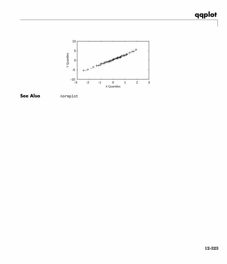
qqplot
See Also normplot
-3 -2 -1 0 1 2 3-10
-5
0
5
10
X Quantiles
Y Q
uant
iles
12-323

random
12randomPurpose Random numbers from a specified distribution
Syntax y = random('name',A1,A2,A3,m,n)
Description y = random('name',A1,A2,A3,m,n) returns a matrix of random numbers, where 'name' is a string containing the name of the distribution, and A1, A2, and A3 are matrices of distribution parameters. Depending on the distribution some of the parameters may not be necessary.
Vector or matrix inputs must all have the same size. A scalar input is expanded to a constant matrix with the same dimensions as the other inputs.
The last two parameters, d and e, are the size of the matrix y. If the distribution parameters are matrices, then these parameters are optional, but they must match the size of the other matrix arguments (see second example).
random is a utility routine allowing you to access all the random number generators in the Statistics Toolbox using the name of the distribution as a parameter. See “Overview of the Distributions” on page 2-11 for the list of available distributions.
Examples rn = random('Normal',0,1,2,4)
rn = 1.1650 0.0751 -0.6965 0.0591 0.6268 0.3516 1.6961 1.7971
rp = random('Poisson',1:6,1,6)
rp = 0 0 1 2 5 7
See Also betarnd, binornd, cdf, chi2rnd, exprnd, frnd, gamrnd, geornd, hygernd, icdf, lognrnd, nbinrnd, ncfrnd, nctrnd, ncx2rnd, normrnd, pdf, poissrnd, raylrnd, trnd, unidrnd, unifrnd, weibrnd
12-324

randtool
12randtoolPurpose Interactive random number generation using histograms for display
Syntax randtoolr = randtool('output')
Description The randtool command sets up a graphic user interface for exploring the effects of changing parameters and sample size on the histogram of random samples from the supported probability distributions.
The M-file calls itself recursively using the action and flag parameters. For general use call randtool without parameters.
To output the current set of random numbers, press the Output button. The results are stored in the variable ans. Alternatively, use the following command.
r = randtool('output') places the sample of random numbers in the vector r.
To sample repetitively from the same distribution, press the Resample button.
To change the distribution function, choose from the pop-up menu of functions at the top of the figure.
To change the parameter settings, move the sliders or type a value in the edit box under the name of the parameter. To change the limits of a parameter, type a value in the edit box at the top or bottom of the parameter slider.
To change the sample size, type a number in the Sample Size edit box.
When you are done, press the Close button.
For an extensive discussion, see “The randtool Demo” on page 11-18.
See Also disttool
12-325

range
12rangePurpose Sample range
Syntax y = range(X)
Description range(X) returns the difference between the maximum and the minimum of a sample. For vectors, range(x) is the range of the elements. For matrices, range(X) is a row vector containing the range of each column of X.
The range is an easily calculated estimate of the spread of a sample. Outliers have an undue influence on this statistic, which makes it an unreliable estimator.
Example The range of a large sample of standard normal random numbers is approximately six. This is the motivation for the process capability indices Cp and Cpk in statistical quality control applications.
rv = normrnd(0,1,1000,5);near6 = range(rv)
near6 =
6.1451 6.4986 6.2909 5.8894 7.0002
See Also std, iqr, mad
12-326

ranksum
12ranksumPurpose Wilcoxon rank sum test that two populations are identical
Syntax p = ranksum(x,y,alpha)[p,h] = ranksum(x,y,alpha)[p,h,stats] = ranksum(x,y,alpha)
Description p = ranksum(x,y,alpha) returns the significance probability that the populations generating two independent samples, x and y, are identical. x and y are both vectors, but can have different lengths. alpha is the desired level of significance and must be a scalar between zero and one.
[p,h] = ranksum(x,y,alpha) also returns the result of the hypothesis test, h. h is zero if the populations of x and y are not significantly different. h is one if the two populations are significantly different.
p is the probability of observing a result equally or more extreme than the one using the data (x and y) if the null hypothesis is true. If p is near zero, this casts doubt on this hypothesis.
[p,h,stats] = ranksum(x,y,alpha) also returns a structure containing the field stats.ranksum whose value is equal to the rank sum statistic. For large samples, it also contains stats.zval that is the value of the normal (Z) statistic used to compute p.
Example This example tests the hypothesis of equality of means for two samples generated with poissrnd.
x = poissrnd(5,10,1);y = poissrnd(2,20,1);[p,h] = ranksum(x,y,0.05)
p = 0.0027
h = 1
See Also signrank, signtest, ttest2
12-327

raylcdf
12raylcdfPurpose Rayleigh cumulative distribution function (cdf)
Syntax P = raylcdf(X,B)
Description P = raylcdf(X,B) computes the Rayleigh cdf at each of the values in X using the corresponding parameters in B. Vector or matrix inputs for X and B must have the same size, which is also the size of P. A scalar input for X or B is expanded to a constant matrix with the same dimensions as the other input.
The Rayleigh cdf is
Example x = 0:0.1:3;p = raylcdf(x,1);plot(x,p)
Reference [1] Evans, M., N. Hastings, and B. Peacock, Statistical Distributions, Second Edition, Wiley 1993. pp. 134–136.
See Also cdf, raylinv, raylpdf, raylrnd, raylstat
y F x b( ) t
b2------
0
x
∫ e
t2–
2b2---------
= = dt
0 0.5 1 1.5 2 2.5 30
0.2
0.4
0.6
0.8
1
12-328

raylinv
12raylinvPurpose Inverse of the Rayleigh cumulative distribution function
Syntax X = raylinv(P,B)
Description X = raylinv(P,B) returns the inverse of the Rayleigh cumulative distribution function with parameter B at the corresponding probabilities in P. Vector or matrix inputs for P and B must have the same size, which is also the size of X. A scalar input for P or B is expanded to a constant matrix with the same dimensions as the other input.
Example x = raylinv(0.9,1)
x = 2.1460
See Also icdf, raylcdf, raylpdf, raylrnd, raylstat
12-329

raylpdf
12raylpdfPurpose Rayleigh probability density function
Syntax Y = raylpdf(X,B)
Description Y = raylpdf(X,B) computes the Rayleigh pdf at each of the values in X using the corresponding parameters in B. Vector or matrix inputs for X and B must have the same size, which is also the size of Y. A scalar input for X or B is expanded to a constant matrix with the same dimensions as the other input.
The Rayleigh pdf is
Example x = 0:0.1:3;p = raylpdf(x,1);plot(x,p)
See Also pdf, raylcdf, raylinv, raylrnd, raylstat
y f x b( ) x
b2------e
x2–
2b2---------
= =
0 0.5 1 1.5 2 2.5 30
0.2
0.4
0.6
0.8
12-330

raylrnd
12raylrndPurpose Random matrices from the Rayleigh distribution
Syntax R = raylrnd(B)R = raylrnd(B,m)R = raylrnd(B,m,n)
Description R = raylrnd(B) returns a matrix of random numbers chosen from the Rayleigh distribution with parameter B. The size of R is the size of B.
R = raylrnd(B,m) returns a matrix of random numbers chosen from the Rayleigh distribution with parameter B, where m is a 1-by-2 vector that contains the row and column dimensions of R.
R = raylrnd(B,m,n) returns a matrix of random numbers chosen from the Rayleigh distribution with parameter B, where scalars m and n are the row and column dimensions of R.
Example r = raylrnd(1:5)
r = 1.7986 0.8795 3.3473 8.9159 3.5182
See Also random, raylcdf, raylinv, raylpdf, raylstat
12-331

raylstat
12raylstatPurpose Mean and variance for the Rayleigh distribution
Syntax M = raylstat(B)[M,V] = raylstat(B)
Description [M,V] = raylstat(B) returns the mean and variance of the Rayleigh distribution with parameter B.
The mean of the Rayleigh distribution with parameter b is and the variance is
Example [mn,v] = raylstat(1)
mn = 1.2533
v = 0.4292
See Also raylcdf, raylinv, raylpdf, raylrnd
b π 2⁄
4 π–2------------b2
12-332

rcoplot
12rcoplotPurpose Residual case order plot
Syntax rcoplot(r,rint)
Description rcoplot(r,rint) displays an errorbar plot of the confidence intervals on the residuals from a regression. The residuals appear in the plot in case order. Inputs r and rint are outputs from the regress function.
Example X = [ones(10,1) (1:10)'];y = X ∗ [10;1] + normrnd(0,0.1,10,1);[b,bint,r,rint] = regress(y,X,0.05);rcoplot(r,rint);
The figure shows a plot of the residuals with error bars showing 95% confidence intervals on the residuals. All the error bars pass through the zero line, indicating that there are no outliers in the data.
See Also regress
0 2 4 6 8 10
-0.2
-0.1
0
0.1
0.2
Res
idua
ls
Case Number
12-333
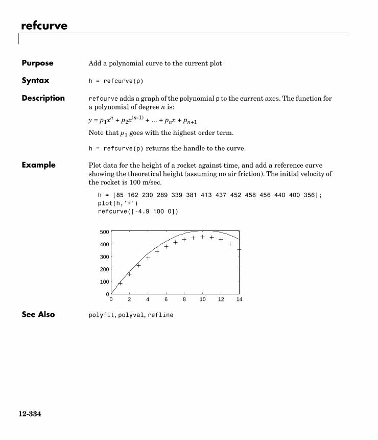
refcurve
12refcurvePurpose Add a polynomial curve to the current plot
Syntax h = refcurve(p)
Description refcurve adds a graph of the polynomial p to the current axes. The function for a polynomial of degree n is:
y = p1xn + p2x(n-1) + ... + pnx + pn+1
Note that p1 goes with the highest order term.
h = refcurve(p) returns the handle to the curve.
Example Plot data for the height of a rocket against time, and add a reference curve showing the theoretical height (assuming no air friction). The initial velocity of the rocket is 100 m/sec.
h = [85 162 230 289 339 381 413 437 452 458 456 440 400 356];plot(h,'+')refcurve([-4.9 100 0])
See Also polyfit, polyval, refline
0 2 4 6 8 10 12 140
100
200
300
400
500
12-334

refline
12reflinePurpose Add a reference line to the current axes
Syntax refline(slope,intercept)refline(slope)h = refline(slope,intercept)refline
Description refline(slope,intercept) adds a reference line with the given slope and intercept to the current axes.
refline(slope), where slope is a two-element vector, adds the line
y = slope(2) + slope(1)*x
to the figure.
h = refline(slope,intercept) returns the handle to the line.
refline with no input arguments superimposes the least squares line on each line object in the current figure (except LineStyles '-','--','.-'). This behavior is equivalent to lsline.
Example y = [3.2 2.6 3.1 3.4 2.4 2.9 3.0 3.3 3.2 2.1 2.6]';plot(y,'+')refline(0,3)
See Also lsline, polyfit, polyval, refcurve
0 2 4 6 8 10 122
2.5
3
3.5
12-335

regress
12regressPurpose Multiple linear regression
Syntax b = regress(y,X)[b,bint,r,rint,stats] = regress(y,X)[b,bint,r,rint,stats] = regress(y,X,alpha)
Description b = regress(y,X) returns the least squares fit of y on X by solving the linear model
for β, where:
• y is an n-by-1 vector of observations
• X is an n-by-p matrix of regressors
• β is a p-by-1 vector of parameters
• ε is an n-by-1 vector of random disturbances
[b,bint,r,rint,stats] = regress(y,X) returns an estimate of β in b, a 95% confidence interval for β in the p-by-2 vector bint. The residuals are returned in r and a 95% confidence interval for each residual is returned in the n-by-2 vector rint. The vector stats contains the R2 statistic along with the F and p values for the regression.
[b,bint,r,rint,stats] = regress(y,X,alpha) gives 100(1-alpha)% confidence intervals for bint and rint. For example, alpha = 0.2 gives 80% confidence intervals.
Examples Suppose the true model is
where I is the identity matrix.
X = [ones(10,1) (1:10)']
X = 1 1
y Xβ ε+=
ε N 0 σ2I,( )∼
y 10 x ε+ +=
ε N 0 0.01I,( )∼
12-336

regress
1 2 1 3 1 4 1 5 1 6 1 7 1 8 1 9 1 10
y = X ∗ [10;1] + normrnd(0,0.1,10,1)
y = 11.1165 12.0627 13.0075 14.0352 14.9303 16.1696 17.0059 18.1797 19.0264 20.0872
[b,bint] = regress(y,X,0.05)
b = 10.0456 1.0030
bint = 9.9165 10.1747 0.9822 1.0238
Compare b to [10 1]'. Note that bint includes the true model values.
Reference [1] Chatterjee, S. and A. S. Hadi. Influential Observations, High Leverage Points, and Outliers in Linear Regression. Statistical Science, 1986. pp. 379–416.
12-337

regstats
12regstatsPurpose Regression diagnostics for linear models
Syntax regstats(responses,DATA,'model')'stats = regstats(responses,DATA,'model','whichstats')
Description regstats(responses,data,'model') fits a multiple regression of the measurements in the vector, responses, on the values in the matrix, DATA. The function creates a UI that displays a group of checkboxes that save diagnostic statistics to the base workspace using specified variable names. 'model' controls the order of the regression model. By default, regstats uses a linear additive model with a constant term.
'model' can be one of the following strings
The order of the coefficients is the order defined by the x2fx function.
stats = regstats(responses,DATA,model,whichstats) creates an output structure stats containing the statistics listed in 'whichstats'. 'whichstats' can be a single name such as 'leverage' or a cell array of names such as {'leverage' 'standres' 'studres'}. Valid names are:
'linear' Includes constant and linear terms (default).
'interaction' Includes constant, linear, and cross product terms.
'quadratic' Includes interactions and squared terms.
'purequadratic' Includes constant, linear, and squared terms.
'Q' Q from the QR Decomposition of X
'R' R from the QR Decomposition of X
'beta' Regression Coefficients
'covb' Covariance of Regression Coefficients
'yhat' Fitted Values of the Response Data
'r' Residuals
'mse' Mean Squared Error
'leverage' Leverage
12-338

regstats
For more detail press the Help button in the regstats window. This provides formulae and interpretations for each of these regression diagnostics.
Algorithm The usual regression model is y = Xβ + ε, where:
• y is an n-by-1 vector of responses
• X is an n-by-p matrix of predictors
• β is an p-by-1 vector of parameters
• ε is an n-by-1 vector of random disturbances
Let X = Q*R where Q and R come from a QR Decomposition of X. Q is orthogonal and R is triangular. Both of these matrices are useful for calculating many regression diagnostics (Goodall 1993).
The standard textbook equation for the least squares estimator of β is
However, this definition has poor numeric properties. Particularly dubious is the computation of , which is both expensive and imprecise.
Numerically stable MATLAB code for β is
'hatmat' Hat (Projection) Matrix
's2_i' Delete-1 Variance
'beta_i' Delete-1 Coefficients
'standres' Standardized Residuals
'studres' Studentized Residuals
'dfbetas' Scaled Change in Regression Coefficients
'dffit' Change in Fitted Values
'dffits' Scaled Change in Fitted Values
'covratio' Change in Covariance
'cookd' Cook's Distance
'all' Create all of the above statistics
β� b X'X( ) 1– X'y= =
X'X( ) 1–
12-339

regstats
b = R\(Q'*y);
See Also leverage, stepwise, regress
Reference [1] Belsley, D.A., E. Kuh, and R.E. Welsch , Regression Diagnostics, New York: Wiley, 1980.
[2] Cook, R.D., and S. Weisberg, Residuals and Influence in Regression, New York: Wiley, 1982.
[3] Goodall, C. R., “Computation using the QR decomposition,” Statistical Computing (C. R. Rao, ed.), Handbook in Statistics, Volume 9. Amsterdam, NL Elsevier/North-Holland, 1993.
12-340

ridge
12ridgePurpose Parameter estimates for ridge regression
Syntax b = ridge(y,X,k)
Description b = ridge(y,X,k) returns the ridge regression coefficients b for the linear model y = Xβ + ε, where:
• X is an n-by-p matrix
• y is the n-by-1 vector of observations
• k is a scalar constant (the ridge parameter)
The ridge estimator of β is .
When k = 0, b is the least squares estimator. For increasing k, the bias of b increases, but the variance of b falls. For poorly conditioned X, the drop in the variance more than compensates for the bias.
Example This example shows how the coefficients change as the value of k increases, using data from the hald dataset.
load hald;b = zeros(4,100);kvec = 0.01:0.01:1;count = 0;
for k = 0.01:0.01:1count = count + 1;b(:,count) = ridge(heat,ingredients,k);end
plot(kvec',b'),xlabel('k'),ylabel('b','FontName','Symbol')
b X'X kI+( ) 1– X'y=
12-341

ridge
See Also regress, stepwise
0 0.2 0.4 0.6 0.8 1-10
-5
0
5
10
k
β
12-342

robustdemo
12robustdemoPurpose Demo of robust regression
Syntax robustdemorobustdemo(X,Y)
Description rsmdemo demonstrates robust regression and ordinary least squares regression on a sample dataset. The function creates a figure window containing a scatter plot of sample data vectors X and Y, along with two fitted lines calculated using least squares and the robust bisquare method. The bottom of the figure shows the equations of the lines and the estimated error standard deviations for each fit. If you use the left mouse button to select an point and move it to a new location, both fits will update. If you hold down the right mouse button over any point, the point will be labeled with the leverage of that point on the least squares fit, and the weight of that point in the robust fit.
rsmdemo(X,Y) performs the same demonstration using the X and Y values that you specify.
Example See “The robustdemo Demo” on page 11-22.
See Also robustfit, leverage
12-343

robustfit
12robustfitPurpose Robust regression
Syntax b = robustfit(X,Y)[b,stats] = robustfit(X,Y)[b,stats] = robustfit(X,Y,'wfun',tune,'const')
Description b = robustfit(X,Y) uses robust regression to fit Y as a function of the columns of X, and returns the vector b of coefficient estimates. The robustfit function uses an iteratively reweighted least squares algorithm, with the weights at each iteration calculated by applying the bisquare function to the residuals from the previous iteration. This algorithm gives lower weight to points that do not fit well. The results are less sensitive to outliers in the data as compared with ordinary least squares regression.
[b,stats] = robustfit(X,Y) also returns a stats structure with the following fields:
• stats.ols_s sigma estimate (rmse) from least squares fit
• stats.robust_s robust estimate of sigma
• stats.mad_s estimate of sigma computed using the median absolute deviation of the residuals from their median; used for scaling residuals during the iterative fitting
• stats.s final estimate of sigma, the larger of robust_s and a weighted average of ols_s and robust_s
• stats.se standard error of coefficient estimates
• stats.t ratio of b to stats.se
• stats.p p-values for stats.t
• stats.coeffcorr estimated correlation of coefficient estimates
• stats.w vector of weights for robust fit
• stats.h vector of leverage values for least squares fit
• stats.dfe degrees of freedom for error
• stats.R R factor in QR decomposition of X matrix
The robustfit function estimates the variance-covariance matrix of the coefficient estimates as V = inv(X'*X)*stats.s^2. The standard errors and correlations are derived from V.
12-344

robustfit
[b,stats] = robustfit(X,Y,'wfun',tune,'const') specifies a weight function, a tuning constant, and the presence or absence of a constant term. The weight function 'wfun' can be any of the names listed in the following table.
The value r in the weight function expression is equal to
resid/(tune*s*sqrt(1-h))
where resid is the vector of residuals from the previous iteration, tune is the tuning constant, h is the vector of leverage values from a least squares fit, and s is an estimate of the standard deviation of the error term.
s = MAD/0.6745
The quantity MAD is the median absolute deviation of the residuals from their median. The constant 0.6745 makes the estimate unbiased for the normal distribution. If there are p columns in the X matrix (including the constant term, if any), the smallest p-1 absolute deviations are excluded when computing their median.
In addition to the function names listed above, 'wfun' can be 'ols' to perform unweighted ordinary least squares.
Table 12-2:
Weight function Meaning Tuning constant
'andrews' w = (abs(r)<pi) .* sin(r) ./ r 1.339
'bisquare' w = (abs(r)<1) .* (1 - r.^2).^2 4.685
'cauchy' w = 1 ./ (1 + r.^2) 2.385
'fair' w = 1 ./ (1 + abs(r)) 1.400
'huber' w = 1 ./ max(1, abs(r)) 1.345
'logistic' w = tanh(r) ./ r 1.205
'talwar' w = 1 * (abs(r)<1) 2.795
'welsch' w = exp(-(r.^2)) 2.985
12-345

robustfit
The argument tune overrides the default tuning constant from the table. A smaller tuning constant tends to downweight large residuals more severely, and a larger tuning constant downweights large residuals less severely. The default tuning constants, shown in the table, yield coefficient estimates that are approximately 95% as efficient as least squares estimates, when the response has a normal distribution with no outliers. The value of 'const' can be 'on' (the default) to add a constant term or 'off' to omit it. If you want a constant term, you should set 'const' to 'on' rather than adding a column of ones to your X matrix.
As an alternative to specifying one of the named weight functions shown above, you can write your own weight function that takes a vector of scaled residuals as input and produces a vector of weights as output. You can specify 'wfun' using @ (for example, @myfun) or as an inline function.
Example Let’s see how a single erroneous point affects least squares and robust fits. First we generate a simple dataset following the equation y = 10-2*x plus some random noise. Then we change one y value to simulate an outlier that could be an erroneous measurement.
x = (1:10)';y = 10 - 2*x + randn(10,1);y(10) = 0;
We use both ordinary least squares and robust fitting to estimate the equations of a straight line fit.
bls = regress(y,[ones(10,1) x])
bls =
8.6305 -1.4721
brob = robustfit(x,y)
brob =
10.5089 -1.9844
12-346

robustfit
A scatter plot with both fitted lines shows that the robust fit (solid line) fits most of the data points well but ignores the outlier. The least squares fit (dotted line) is pulled toward the outlier.
scatter(x,y)hold onplot(x,bls(1)+bls(2)*x,'g:')plot(x,brob(1)+brob(2)*x,'r-')
See Also regress, robustdemo
References [1] DuMouchel, W.H., and F.L. O’Brien (1989), “Integrating a Robust Option into a Multiple Regression Computing Environment,” Computer Science and Statistics: Proceedings of the 21st Symposium on the Interface, Alexandria, VA: American Statistical Association.
[2] Holland, P.W., and R.E. Welsch (1977), “Robust Regression Using Iteratively Reweighted Least-Squares,” Communications in Statistics: Theory and Methods, A6, 813-827.
[3] Huber, P.J. (1981), Robust Statistics, New York: Wiley.
[4] Street, J.O., R.J. Carroll, and D. Ruppert (1988), “A Note on Computing Robust Regression Estimates via Iteratively Reweighted Least Squares,” The American Statistician, 42, 152-154
1 2 3 4 5 6 7 8 9 10−10
−8
−6
−4
−2
0
2
4
6
8
10
12-347

rowexch
12rowexchPurpose D-optimal design of experiments – row exchange algorithm
Syntax settings = rowexch(nfactors,nruns)[settings,X] = rowexch(nfactors,nruns)[settings,X] = rowexch(nfactors,nruns,'model')[settings,X] = rowexch(...,'param1',value1,'param2',value2,...)
Description settings = rowexch(nfactors,nruns) generates the factor settings matrix, settings, for a D-Optimal design using a linear additive model with a constant term. settings has nruns rows and nfactors columns.
[settings,X] = rowexch(nfactors,nruns) also generates the associated matrix X of term settings, often called the design matrix.
[settings,X] = rowexch(nfactors,nruns,'model') produces a design for fitting a specified regression model. The input, 'model', can be one of these strings:
[settings,X] = rowexch(...,'param1',value1,'param2',value2,...)provides more control over the design generation through a set of parameter/value pairs. Valid parameters are:
Example This example illustrates that the D-optimal design for three factors in eight runs, using an interactions model, is a two level full-factorial design.
'linear' Includes constant and linear terms (the default)
'interaction' Includes constant, linear, and cross product terms.
'quadratic' Includes interactions plus squared terms.
'purequadratic' Includes constant, linear and squared terms.
'display' Either 'on' or 'off' to control display of iteration counter. The default is 'on'.
'init' Initial design as an nruns-by-nfactors matrix. The default is a randomly selected set of points.
'maxiter' Maximum number of iterations. The default is 10.
12-348

rowexch
s = rowexch(3,8,'interaction')
s = -1 -1 1 1 -1 -1 1 -1 1 -1 -1 -1 -1 1 1 1 1 1 -1 1 -1 1 1 -1
Algorithm The rowexch function searches for a D-optimal design using a row-exchange algorithm. It first generates a candidate set of points that are eligible to be included in the design, and then iteratively exchanges design points for candidate points in an attempt to reduce the variance of the coefficients that would be estimated using this design. If you need to use a candidate set that differs from the default one, call the candgen and candexch functions in place of rowexch.
See Also bbdesign, candexch, candgen, ccdesign, cordexch, x2fx
12-349

rsmdemo
12rsmdemoPurpose Demo of design of experiments and surface fitting
Syntax rsmdemo
Description rsmdemo creates a GUI that simulates a chemical reaction. To start, you have a budget of 13 test reactions. Try to find out how changes in each reactant affect the reaction rate. Determine the reactant settings that maximize the reaction rate. Estimate the run-to-run variability of the reaction. Now run a designed experiment using the model pop-up. Compare your previous results with the output from response surface modeling or nonlinear modeling of the reaction. The GUI has the following elements:
• A Run button to perform one reactor run at the current settings
• An Export button to export the x and y data to the base workspace
• Three sliders with associated data entry boxes to control the partial pressures of the chemical reactants: Hydrogen, n-Pentane, and Isopentane
• A text box to report the reaction rate
• A text box to keep track of the number of test reactions you have left
Example See “The rsmdemo Demo” on page 11-19.
See Also rstool, nlintool, cordexch
12-350

rstool
12rstoolPurpose Interactive fitting and visualization of a response surface
Syntax rstool(x,y)rstool(x,y,'model')rstool(x,y,'model',alpha,'xname','yname')
Description rstool(x,y) displays an interactive prediction plot with 95% global confidence intervals. This plot results from a multiple regression of (x,y) data using a linear additive model.
rstool(x,y,'model') allows control over the initial regression model, where 'model' can be one of the following strings:
• 'interaction' – includes constant, linear, and cross product terms
• 'quadratic' – includes interactions and squared terms
• 'purequadratic' – includes constant, linear and squared terms
rstool(x,y,'model',alpha) plots 100(1-alpha)% global confidence interval for predictions as two red curves. For example, alpha = 0.01 gives 99% confidence intervals.
rstool displays a “vector” of plots, one for each column of the matrix of inputs x. The response variable, y, is a column vector that matches the number of rows in x.
rstool(x,y,'model',alpha,'xname','yname') labels the graph using the string matrix 'xname' for the labels to the x-axes and the string, 'yname', to label the y-axis common to all the plots.
Drag the dotted white reference line and watch the predicted values update simultaneously. Alternatively, you can get a specific prediction by typing the value of x into an editable text field. Use the pop-up menu labeled Model to interactively change the model. Use the pop-up menu labeled Export to move specified variables to the base workspace.
Example See “Quadratic Response Surface Models” on page 4-22.
See Also nlintool
12-351

schart
12schartPurpose Chart of standard deviation for Statistical Process Control
Syntax schart(DATA,conf)schart(DATA,conf,specs)schart(DATA,conf,specs)[outliers,h] = schart(DATA,conf,specs)
Description schart(data) displays an S chart of the grouped responses in DATA. The rows of DATA contain replicate observations taken at a given time. The rows must be in time order. The graph contains the sample standard deviation s for each group, a center line at the average s value, and upper and lower control limits. The limits are placed at a three-sigma distance on either side of the center line, where sigma is an estimate of the standard deviation of s. If the process is in control, fewer than 3 out of 1000 observations would be expected to fall outside the control limits by random chance. So, if you observe points outside the limits, you can take this as evidence that the process is not in control.
schart(DATA,conf) allows control of the confidence level of the upper and lower plotted control limits. The default conf = 0.9973 produces three-sigma limits.
norminv(1 - (1-.9973)/2)ans = 3
To get k-sigma limits, use the expression 1-2*(1-normcdf(k)). For example, the correct conf value for 2-sigma limits is 0.9545, as shown below.
k = 2;1-2*(1-normcdf(k))ans = 0.9545
schart(DATA,conf,specs) plots the specification limits in the two element vector specs.
[outliers,h] = schart(data,conf,specs) returns outliers, a vector of indices to the rows where the mean of DATA is out of control, and h, a vector of handles to the plotted lines.
12-352

schart
Example This example plots an S chart of measurements on newly machined parts, taken at one hour intervals for 36 hours. Each row of the runout matrix contains the measurements for 4 parts chosen at random. The values indicate, in thousandths of an inch, the amount the part radius differs from the target radius.
load partsschart(runout)
All points are within the control limits, so the variability within subgroups is consistent with what would be expected by random chance. There is no evidence that the process is out of control.
Reference [1] Montgomery, D., Introduction to Statistical Quality Control, John Wiley and Sons 1991. p. 235.
See Also capaplot, ewmaplot, histfit, xbarplot
0 5 10 15 20 25 30 35 400
0.05
0.1
0.15
0.2
0.25
0.3
0.35
UCL
LCL
CL
S Chart
Sample Number
Sta
ndar
d D
evia
tion
12-353

signrank
12signrankPurpose Wilcoxon signed rank test of equality of medians
Syntax p = signrank(x,y,alpha)[p,h] = signrank(x,y,alpha)[p,h,stats] = signrank(x,y,alpha)
Description p = signrank(x,y,alpha) returns the significance probability that the medians of two matched samples, x and y, are equal. x and y must be vectors of equal length. y may also be a scalar; in this case, signrank computes the probability that the median of x is different from the constant y. alpha is the desired level of significance, and must be a scalar between zero and one.
[p,h] = signrank(x,y,alpha) also returns the result of the hypothesis test, h. h is zero if the difference in medians of x and y is not significantly different from zero. h is one if the two medians are significantly different.
p is the probability of observing a result equally or more extreme than the one using the data (x and y) if the null hypothesis is true. p is calculated using the rank values for the differences between corresponding elements in x and y. If p is near zero, this casts doubt on this hypothesis.
[p,h,stats] = signrank(x,y,alpha) also returns a structure stats containing the field stats.signedrank whose value is the signed rank statistic. For large samples, it also contains stats.zval, the value of the normal (Z) statistic used to compute p.
Example This example tests the hypothesis of equality of means for two samples generated with normrnd. The samples have the same theoretical mean but different standard deviations.
x = normrnd(0,1,20,1);y = normrnd(0,2,20,1);[p,h] = signrank(x,y,0.05)
p = 0.2959
h = 0
12-354

signrank
See Also ranksum, signtest, ttest
12-355

signtest
12signtestPurpose Sign test for paired samples
Syntax p = signtest(x,y,alpha)[p,h] = signtest(x,y,alpha)[p,h,stats] = signtest(x,y,alpha)
Description p = signtest(x,y,alpha) returns the significance probability that the medians of two matched samples, x and y, are equal. x and y must be vectors of equal length. y may also be a scalar; in this case, signtest computes the probability that the median of x is different from the constant y. alpha is the desired level of significance and must be a scalar between zero and one.
[p,h] = signtest(x,y,alpha) also returns the result of the hypothesis test, h. h is 0 if the difference in medians of x and y is not significantly different from zero. h is 1 if the two medians are significantly different.
p is the probability of observing a result equally or more extreme than the one using the data (x and y) if the null hypothesis is true. p is calculated using the signs (plus or minus) of the differences between corresponding elements in x and y. If p is near zero, this casts doubt on this hypothesis.
[p,h,stats] = signtest(x,y,alpha) also returns a structure stats containing the field stats.sign whose value is the sign statistic. For large samples, it also contains stats.zval, the value of the normal (Z) statistic used to compute p.
Example This example tests the hypothesis of equality of medians for two samples generated with normrnd. The samples have the same theoretical median but different standard deviations. (For the normal distribution, the mean and median are the same.)
x = normrnd(0,1,20,1);y = normrnd(0,2,20,1);[p,h] = signtest(x,y,0.05)
p = 0.2632
h = 0
12-356

signtest
See Also ranksum, signrank, ttest
12-357
silhouette
12silhouettePurpose Silhouette plot for clustered data
Syntax silhouette(X,clust)s = silhouette(X,clust)[s,h] = silhouette(X,clust)[...] = silhouette(X,clust,distance)[...] = silhouette(X,clust,distfun,p1,p2,...)
Description silhouette(X,clust) plots cluster silhouettes for the n-by-p data matrix X, with clusters defined by clust. Rows of X correspond to points, columns correspond to coordinates. clust can be a numeric vector containing a cluster index for each point, or a character matrix or cell array of strings containing a cluster name for each point. silhouette treats NaNs or empty strings in clust as missing values, and ignores the corresponding rows of X. By default, silhouette uses the squared Euclidean distance between points in X.
s = silhouette(X,clust) returns the silhouette values in the n-by-1 vector s, but does not plot the cluster silhouettes.
[s,h] = silhouette(X,clust) plots the silhouettes, and returns the silhouette values in the n-by-1 vector s, and the figure handle in h.
[...] = silhouette(X,clust,distance) plots the silhouettes using the inter-point distance measure specified in distance. Choices for distance are:
'Euclidean' Euclidean distance
'sqEuclidean' Squared Euclidean distance (default)
'cityblock' Sum of absolute differences, i.e., L1
'cosine' One minus the cosine of the included angle between points (treated as vectors)
'correlation' One minus the sample correlation between points (treated as sequences of values)
'Hamming' Percentage of coordinates that differ
12-358
silhouette
[...] = silhouette(X,clust,distfun,p1,p2, ...) accepts a distance function of the form
d = distfun(X0,X,p1,p2,...)
where X0 is a 1-by-p point, X is an n-by-p matrix of points, and p1,p2,... are optional additional arguments. The function distfun returns an n-by-1 vector d of distances between X0 and each point (row) in X. The arguments p1, p2,... are passed directly to the function distfun.
Remarks The silhouette value for each point is a measure of how similar that point is to points in its own cluster compared to points in other clusters, and ranges from -1 to +1. It is defined as
S(i) = (min(b(i,:),2) - a(i)) ./ max(a(i),min(b(i,:),2))
where a(i) is the average distance from the ith point to the other points in its cluster, and b(i,k) is the average distance from the ith point to points in another cluster k.
Examples X = [randn(10,2)+ones(10,2); randn(10,2)-ones(10,2)];cidx = kmeans(X,2,'distance','sqeuclid');s = silhouette(X,cidx,'sqeuclid');
See Also dendrogram, kmeans, linkage, pdist
References [1] Kaufman L. and P.J. Rousseeuw, Finding Groups in Data: An Introduction to Cluster Analysis, Wiley, 1990
'Jaccard' Percentage of non-zero coordinates that differ
Vector A numeric distance matrix in upper triangular vector form, such as is created by pdist. X is not used in this case, and can safely be set to [].
12-359

skewness
12skewnessPurpose Sample skewness
Syntax y = skewness(X)y = skewness(X,flag)
Description y = skewness(X) returns the sample skewness of X. For vectors, skewness(x) is the skewness of the elements of x. For matrices, skewness(X) is a row vector containing the sample skewness of each column.
Skewness is a measure of the asymmetry of the data around the sample mean. If skewness is negative, the data are spread out more to the left of the mean than to the right. If skewness is positive, the data are spread out more to the right. The skewness of the normal distribution (or any perfectly symmetric distribution) is zero.
The skewness of a distribution is defined as
where µ is the mean of x, σ is the standard deviation of x, and E(t) represents the expected value of the quantity t.
y = skewness(X,flag) specifies whether to correct for bias (flag = 0) or not (flag = 1, the default). When X represents a sample from a population, the skewness of X is biased; that is, it will tend to differ from the population skewness by a systematic amount that depends on the size of the sample. You can set flag = 0 to correct for this systematic bias.
Example X = randn([5 4])
X = 1.1650 1.6961 -1.4462 -0.3600 0.6268 0.0591 -0.7012 -0.1356 0.0751 1.7971 1.2460 -1.3493 0.3516 0.2641 -0.6390 -1.2704 -0.6965 0.8717 0.5774 0.9846
y = skewness(X)
y =
y E x µ–( )3
σ3------------------------=
12-360

skewness
-0.2933 0.0482 0.2735 0.4641
See Also kurtosis, mean, moment, std, var
12-361

squareform
12squareform
Purpose Reformat the output of pdist into a square matrix.
Syntax S = squareform(Y)
Description S = squareform(Y) reformats the distance information returned by pdist from a vector into a square matrix. In this format, S(i,j) denotes the distance between the i and j observations in the original data.
See Also pdist
12-362

std
12stdPurpose Standard deviation of a sample
Syntax y = std(X)
Description y = std(X) computes the sample standard deviation of the data in X. For vectors, std(x) is the standard deviation of the elements in x. For matrices, std(X) is a row vector containing the standard deviation of each column of X.
std normalizes by n-1 where n is the sequence length. For normally distributed data, the square of the standard deviation is the minimum variance unbiased estimator of σ 2 (the second parameter).
The standard deviation is
where the sample average is .
The std function is part of the standard MATLAB language.
Examples In each column, the expected value of y is one.
x = normrnd(0,1,100,6);y = std(x)
y = 0.9536 1.0628 1.0860 0.9927 0.9605 1.0254
y = std(-1:2:1)
y = 1.4142
See Also cov, var
s 1n 1–------------- xi x–( )2
i 1=
n
∑
12---
=
x 1n--- xi∑=
12-363
stepwise
12stepwisePurpose Interactive environment for stepwise regression
Syntax stepwise(X,y)stepwise(X,y,inmodel)stepwise(X,y,inmodel,alpha)
Description stepwise(X,y) fits a regression model of y on the columns of X. It displays three figure windows for interactively controlling the stepwise addition and removal of model terms.
stepwise(X,y,inmodel) allows control of the terms in the original regression model. The values of vector, inmodel, are the indices of the columns of the matrix X to include in the initial model.
stepwise(X,y,inmodel,alpha) allows control of the length confidence intervals on the fitted coefficients. alpha is the significance for testing each term in the model. By default, alpha = 1 - (1 - 0.025)(1/p) where p is the number of columns in X. This translates to plotted 95% simultaneous confidence intervals (Bonferroni) for all the coefficients.
The least squares coefficient is plotted with a green filled circle. A coefficient is not significantly different from zero if its confidence interval crosses the white zero line. Significant model terms are plotted using solid lines. Terms not significantly different from zero are plotted with dotted lines.
Click on the confidence interval lines to toggle the state of the model coefficients. If the confidence interval line is green, the term is in the model. If the confidence interval line is red, the term is not in the model.
Use the Export menu to move variables to the base workspace.
Example See “Stepwise Regression” on page 4-24.
Reference [1] Draper, N. and H. Smith, Applied Regression Analysis, Second Edition, John Wiley and Sons, Inc. 1981 pp. 307–312.
See Also regstats, regress, rstool
12-364

surfht
12surfhtPurpose Interactive contour plot
Syntax surfht(Z)surfht(x,y,Z)
Description surfht(Z) is an interactive contour plot of the matrix Z treating the values in Z as height above the plane. The x-values are the column indices of Z while the y-values are the row indices of Z.
surfht(x,y,Z) where x and y are vectors specify the x and y-axes on the contour plot. The length of x must match the number of columns in Z, and the length of y must match the number of rows in Z.
There are vertical and horizontal reference lines on the plot whose intersection defines the current x-value and y-value. You can drag these dotted white reference lines and watch the interpolated z-value (at the top of the plot) update simultaneously. Alternatively, you can get a specific interpolated z-value by typing the x-value and y-value into editable text fields on the x-axis and y-axis respectively.
12-365

tabulate
12tabulatePurpose Frequency table
Syntax table = tabulate(x)tabulate(x)
Description table = tabulate(x) takes a vector of positive integers, x, and returns a matrix, table.
The first column of table contains the values of x. The second contains the number of instances of this value. The last column contains the percentage of each value.
tabulate with no output arguments displays a formatted table in the command window.
Example tabulate([1 2 4 4 3 4])
Value Count Percent 1 1 16.67% 2 1 16.67% 3 1 16.67% 4 3 50.00%
See Also pareto
12-366
tblread
12tblreadPurpose Read tabular data from the file system
Syntax [data,varnames,casenames] = tblread[data,varnames,casenames] = tblread('filename')[data,varnames,casenames] = tblread('filename','delimiter')
Description [data,varnames,casenames] = tblread displays the File Open dialog box for interactive selection of the tabular data file. The file format has variable names in the first row, case names in the first column and data starting in the (2,2) position.
[data,varnames,casenames] = tblread(filename) allows command line specification of the name of a file in the current directory, or the complete pathname of any file.
[data,varnames,casenames] = tblread(filename,'delimiter') allows specification of the field 'delimiter' in the file. Accepted values are 'tab', 'space', or 'comma'.
tblread returns the data read in three values.
Example [data,varnames,casenames] = tblread('sat.dat')
data =
470 530 520 480
varnames =
Male
Return Value Description
data Numeric matrix with a value for each variable-case pair.
varnames String matrix containing the variable names in the first row.
casenames String matrix containing the names of each case in the first column.
12-367

tblread
Female
casenames =
Verbal Quantitative
See Also caseread, tblwrite, tdfread
12-368

tblwrite
12tblwritePurpose Writes tabular data to the file system
Syntax tblwrite(data,'varnames','casenames')tblwrite(data,'varnames','casenames','filename')
Description tblwrite(data,'varnames','casenames') displays the File Open dialog box for interactive specification of the tabular data output file. The file format has variable names in the first row, case names in the first column and data starting in the (2,2) position.
'varnames' is a string matrix containing the variable names. 'casenames' is a string matrix containing the names of each case in the first column. data is a numeric matrix with a value for each variable-case pair.
tblwrite(data,'varnames','casenames','filename') allows command line specification of a file in the current directory, or the complete pathname of any file in the string 'filename'.
Example Continuing the example from tblread:
tblwrite(data,varnames,casenames,'sattest.dat')type sattest.dat
Male FemaleVerbal 470 530Quantitative 520 480
See Also casewrite, tblread
12-369

tcdf
12tcdfPurpose Student’s t cumulative distribution function (cdf)
Syntax P = tcdf(X,V)
Description P = tcdf(X,V) computes Student’s t cdf at each of the values in X using the corresponding degrees of freedom in V. Vector or matrix inputs for X and V must be the same size. A scalar input is expanded to a constant matrix with the same dimensions as the other inputs. The parameters in V must be positive integers.
The t cdf is
The result, p, is the probability that a single observation from the t distribution with ν degrees of freedom will fall in the interval (-∞ x].
Examples Suppose 10 samples of Guinness beer have a mean alcohol content of 5.5% by volume and the standard deviation of these samples is 0.5%. What is the probability that the true alcohol content of Guinness beer is less than 5%?
t = (5.0 - 5.5) / 0.5;probability = tcdf(t,10 - 1)
probability =
0.1717
See Also cdf, tinv, tpdf, trnd, tstat
p F x ν( )Γ ν 1+
2------------
Γ ν2---
---------------------- 1νπ---------- 1
1 t2
ν-----+
ν 1+2
------------------------------------------- td
∞–
x
∫= =
12-370

tdfread
12tdfreadPurpose Read file containing tab-delimited numeric and text values
Syntax tdfreadtdfread('filename')tdfread('filename','delimiter')
Description tdfread displays the File Open dialog box for interactive selection of the data file. The file should consist of columns of values, separated by tabs, and with column names in the first line of the file. Each column is read from the file and assigned to a variable with the specified name. If all values for a column are numeric, the variable is converted to numbers; otherwise the variable is a string matrix. After all values are imported, tdfread displays information about the imported values using the format of the whos command.
tdfread('filename') allows command line specification of the name of a file in the current directory, or the complete pathname of any file.
tdfread('filename','delimiter') indicates that the character specified by 'delimiter' separates columns in the file. Accepted values are:
• ' ' or 'space'
• '\t' or 'tab'
• ',' or 'comma'
• ';' or 'semi'
• '|' or 'bar'
The default delimiter is 'tab'.
Example type sat2.dat
Test,Gender,ScoreVerbal,Male,470Verbal,Female,530Quantitative,Male,520Quantitative,Female,480tdfread('sat2.dat',',')
Name Size Bytes Class
12-371

tdfread
Gender 4x6 48 char array Score 4x1 32 double array Test 4x12 96 char array
Grand total is 76 elements using 176 bytes
See Also tblread
12-372

tinv
12tinvPurpose Inverse of the Student’s t cumulative distribution function (cdf)
Syntax X = tinv(P,V)
Description X = tinv(P,V) computes the inverse of Student’s t cdf with parameter V for the corresponding probabilities in P. Vector or matrix inputs for P and V must be the same size. A scalar input is expanded to a constant matrix with the same dimensions as the other inputs. The degrees of freedom in V must be positive integers, and the values in P must lie on the interval [0 1].
The t inverse function in terms of the t cdf is
where
The result, x, is the solution of the cdf integral with parameter ν, where you supply the desired probability p.
Examples What is the 99th percentile of the t distribution for one to six degrees of freedom?
percentile = tinv(0.99,1:6)
percentile =
31.8205 6.9646 4.5407 3.7469 3.3649 3.1427
See Also icdf, tcdf, tpdf, trnd, tstat
x F 1– p ν( ) x:F x ν( ) p={ }= =
p F x ν( )Γ ν 1+
2------------
Γ ν2---
---------------------- 1νπ---------- 1
1 t2
ν-----+
ν 1+2
------------------------------------------- td
∞–
x
∫= =
12-373

tpdf
12tpdfPurpose Student’s t probability density function (pdf)
Syntax Y = tpdf(X,V)
Description Y = tpdf(X,V) computes Student’s t pdf at each of the values in X using the corresponding parameters in V. Vector or matrix inputs for X and V must have the same size. A scalar input is expanded to a constant matrix with the same dimensions as the other inputs. The degrees of freedom in V must be positive integers.
Student’s t pdf is
Examples The mode of the t distribution is at x = 0. This example shows that the value of the function at the mode is an increasing function of the degrees of freedom.
tpdf(0,1:6)
ans =
0.3183 0.3536 0.3676 0.3750 0.3796 0.3827
The t distribution converges to the standard normal distribution as the degrees of freedom approaches infinity. How good is the approximation for v = 30?
difference = tpdf(-2.5:2.5,30) - normpdf(-2.5:2.5)
difference =
0.0035 -0.0006 -0.0042 -0.0042 -0.0006 0.0035
See Also pdf, tcdf, tinv, trnd, tstat
y f x ν( )Γ ν 1+
2------------
Γ ν2---
---------------------- 1νπ---------- 1
1 x2
ν-----+
ν 1+2
--------------------------------------------= =
12-374

treedisp
12treedispPurpose Show classification or regression tree graphically
Syntax treedisp(T)treedisp(T,'param1',val1,'param2',val2,...)
Description treedisp(T) takes as input a decision tree T as computed by the treefit function, and displays it in a figure window. Each branch in the tree is labeled with its decision rule, and each terminal node is labeled with the predicted value for that node.
For each branch node, the left child node corresponds to the points that satisfy the condition, and the right child node corresponds to the points that do not satisfy the condition.
The Click to display pop-up menu at the top of the figure enables you to display more information about each node:
After you select the type of information you want, click on any node to display the information for that node.
The Pruning level spin button displays the number of levels that have been cut from the tree, and the number of levels in the unpruned tree. For example, 1 of 6 indicates that the unpruned tree has six levels, and that one level has been cut from the tree. Use the spin button to change the pruning level.
treedisp(T,'param1',val1,'param2',val2,...) specifies optional parameter name-value pairs. Valid parameters are:
Identity The node number, whether the node is a branch or a leaf, and the rule that governs the node
Variable ranges The range of each of the predictor variables for that node
Node statistics The number of elements of the data set that fit the node and ... (the mean and standard deviation of what?)
'names' A cell array of names for the predictor variables, in the order in which they appear in the X matrix from which the tree was created (see treefit)
'prunelevel' Initial pruning level to display
12-375

treedisp
Examples Create and graph classification tree for Fisher's iris data. The names in this example are abbreviations for the column contents (sepal length, sepal width, petal length, and petal width).
load fisheriris; t = treefit(meas,species); treedisp(t,'names',{'SL' 'SW' 'PL' 'PW'});
See Also treefit, treeprune, treetest
12-376

treefit
12treefitPurpose Fit a tree-based model for classification or regression
Syntax T = treefit(X,y)T = treefit(X,y,'param1',val1,'param2',val2,...)
Description T = treefit(X,y) creates a decision tree T for predicting response y as a function of predictors X. X is an n-by-m matrix of predictor values. y is either a vector of n response values (for regression), or a character array or cell array of strings containing n class names (for classification). Either way, T is a binary tree where each non-terminal node is split based on the values of a column of X.
T = treefit(X,y,'param1',val1,'param2',val2,...) specifies optional parameter name-value pairs. Valid parameters are
For all trees:
For classification trees only:
'catidx' Vector of indices of the columns of X. treefit treats these columns as unordered categorical values.
'method' Either 'classification' (default if y is text) or 'regression' (default if y is numeric)
'splitmin' A number n such that impure nodes must have n or more observations to be split (default 10)
'prune' 'on' (default) to compute the full tree and a sequence of pruned subtrees, or 'off' for the full tree without pruning
'cost' p-by-p matrix C, where C(i,j) is the cost of classifying a point into class i if its true class is j (default has C(i,j)=1 if i~=j, and C(i,j)=0 if i=j). C can also be a structure S with two fields : S.group containing the group names, and S.cost containing a matrix of cost values.
12-377

treefit
Examples Create a classification tree for Fisher's iris data.
load fisheriris; t = treefit(meas,species); treedisp(t,'names',{'SL' 'SW' 'PL' 'PW'});
See Also treedisp, treetest
'splitcriterion' Criterion for choosing a split: either 'gdi' (default) for Gini's diversity index, 'twoing' for the twoing rule, or 'deviance' for maximum deviance reduction
'priorprob' Prior probabilities for each class, specified as a vector (one value for each distinct group name) or as a structure S with two fields: S.group containing the group names, and S.prob containing a vector of corresponding probabilities
12-378

treefit
References [1] Breiman, et al., Classification and Regression Trees, Chapman and Hall, Boca Raton, 1993.
12-379

treeprune
12treeprunePurpose Produce a sequence of subtrees by pruning
Syntax T2 = treeprune(T1,'level',level)T2 = treeprune(T1,'nodes',nodes)T2 = treeprune(T1)
Description T2 = treeprune(T1,'level',level) takes a decision tree T1 as created by the treefit function, and a pruning level level, and returns the decision tree T2 pruned to that level. The value level = 0 means no pruning. Trees are pruned based on an optimal pruning scheme that first prunes branches giving less improvement in error cost.
T2 = treeprune(T1,'nodes',nodes) prunes the nodes listed in the nodes vector from the tree. Any T1 branch nodes listed in nodes become leaf nodes in T2, unless their parent nodes are also pruned. The treedisp function can display the node numbers for any node you select.
T2 = treeprune(T1) returns the decision tree T2 that is the same as T1, but with the optimal pruning information added. This is useful only if you created T1 by pruning another tree, or by using the treefit function with pruning set 'off'. If you plan to prune a tree multiple times, it is more efficient to create the optimal pruning sequence first.
Pruning is the process of reducing a tree by turning some branch nodes into leaf nodes, and removing the leaf nodes under the original branch.
Examples Display the full tree for Fisher's iris data, as well as the next largest tree from the optimal pruning sequence.
load fisheriris; t = treefit(meas,species,'splitmin',5); treedisp(t,'names',{'SL' 'SW' 'PL' 'PW'});
12-380

treeprune
t1 = treeprune(t,'level',1); treedisp(t1,'names',{'SL' 'SW' 'PL' 'PW'});
12-381

treeprune
See Also treefit, treetest, treedisp
12-382

treetest
12treetestPurpose Compute error rate for tree
Syntax cost = treetext(T,'resubstitution')cost = treetest(T,'test',X,y)cost = treetest(T,'crossvalidate',X,y)[cost,secost,ntnodes,bestsize] = treetest(...)[...] = treetest(...,'param1',val1,'param2',val2,...)
Description cost = treetext(T,'resubstitution') computes the cost of the tree T using a resubstitution method. T is a decision tree as created by the treefit function. The cost of the tree is the sum over all terminal nodes of the estimated probability of that node times the node's cost. If T is a classification tree, the cost of a node is the sum of of the misclassification costs of the observations in that node. If T is a regression tree, the cost of a node is the average squared error over the observations in that node. cost is a vector of cost values for each subtree in the optimal pruning sequence for T. The resubstitution cost is based on the same sample that was used to create the original tree, so it underestimates the likely cost of applying the tree to new data.
cost = treetest(T,'test',X,y) uses the predictor matrix X and response y as a test sample, applies the decision tree T to that sample, and returns a vector cost of cost values computed for the test sample. X and y should not be the same as the learning sample, which is the sample that was used to fit the tree T.
cost = treetest(T,'crossvalidate',X,y) uses 10-fold cross-validation to compute the cost vector. X and y should be the learning sample, which is the sample that was used to fit the tree T. The function partitions the sample into 10 subsamples, chosen randomly but with roughly equal size. For classification trees, the subsamples also have roughly the same class proportions. For each subsample, treetest fits a tree to the remaining data and uses it to predict the subsample. It pools the information from all subsamples to compute the cost for the whole sample.
[cost,secost,ntnodes,bestlevel] = treetest(...) also returns the vector secost containing the standard error of each cost value, the vector ntnodes containing number of terminal nodes for each subtree, and the scalar
12-383

treetest
bestlevel containing the estimated best level of pruning. bestlevel = 0 means no pruning, i.e., the full unpruned tree. The best level is the one that produces the smallest tree that is within one standard error of the minimum-cost subtree.
[...] = treetest(...,'param1',val1,'param2',val2,...) specifies optional parameter name-value pairs chosen from the following:
Examples Find the best tree for Fisher's iris data using cross-validation. The solid line shows the estimated cost for each tree size, the dashed line marks 1 standard error above the minimum, and the square marks the smallest tree under the dashed line.
% Start with a large tree.load fisheriris;t = treefit(meas,species','splitmin',5);
% Find the minimum-cost tree.[c,s,n,best] = treetest(t,'cross',meas,species);tmin = treeprune(t,'level',best);
% Plot smallest tree within 1 std. error of minimum cost tree.[mincost,minloc] = min(c);plot(n,c,'b-o', n,c+s,'r:', n(best+1),c(best+1),'bs',... n,(mincost+s(minloc))*ones(size(n)),'k--');xlabel('Tree size (number of terminal nodes)')ylabel('Cost')
'nsamples' The number of cross-validations samples (default 10).
'treesize' Either 'se' (default) to choose the smallest tree whose cost is within one standard error of the minimum cost, or 'min' to choose the minimal cost tree.
12-384

treetest
See Also treefit, treedisp
1 2 3 4 5 60
0.1
0.2
0.3
0.4
0.5
0.6
0.7
Tree size (number of terminal nodes)
Cos
t
12-385

treeval
12treevalPurpose Compute fitted value for decision tree applied to data
Syntax YFIT = treeval(T,X)YFIT = treeval(T,X,subtrees)[YFIT,NODE] = treeval(...)[YFIT,NODE,CNAME] = treeval(...)
Description YFIT = treeval(T,X) takes a classification or regression tree T as produced by the treefit function, and a matrix X of predictor values, and produces a vector YFIT of predicted response values. For a regression tree, YFIT(j) is the fitted response value for a point having the predictor values X(j,:). For a classification tree, YFIT(j) is the class number into which the tree would assign the point with data X(j,:). To convert the number into a class name, use the third output argument, cname (below).
YFIT = treeval(T,X,subtrees) takes an additional vector subtrees of pruning levels, with 0 representing the full, unpruned tree. T must include a pruning sequence as created by the treefit or prunetree function. If subtree has k elements and X has n rows, then the output YFIT is an n-by-k matrix, with the jth column containing the fitted values produced by the subtrees(j) subtree. subtrees must be sorted in ascending order.
[YFIT,NODE] = treeval(...) also returns an array NODE of the same size as YFIT containing the node number assigned to each row of X. The treedisp function can display the node numbers for any node you select.
[YFIT,NODE,CNAME] = treeval(...) is valid only for classification trees. It retuns a cell array CNAME containing the predicted class names.
Examples Find the predicted classifications for Fisher's iris data.
load fisheriris;t = treefit(meas,species); % Create decision treesfit = treeval(t,meas); % Find assigned class numberssfit = t.classname(sfit); % Get class namesmean(strcmp(sfit,species)) % Compute proportion correctly % classifiedans = 0.9800
12-386

treeval
See Also treefit, treeprune, treetest
12-387

trimmean
12trimmeanPurpose Mean of a sample of data excluding extreme values
Syntax m = trimmean(X,percent)
Description m = trimmean(X,percent) calculates the mean of a sample X excluding the highest and lowest percent/2 of the observations. The trimmed mean is a robust estimate of the location of a sample. If there are outliers in the data, the trimmed mean is a more representative estimate of the center of the body of the data. If the data is all from the same probability distribution, then the trimmed mean is less efficient than the sample average as an estimator of the location of the data.
Examples This example shows a Monte Carlo simulation of the efficiency of the 10% trimmed mean relative to the sample average for normal data.
x = normrnd(0,1,100,100);m = mean(x);trim = trimmean(x,10);sm = std(m);strim = std(trim);efficiency = (sm/strim).^2
efficiency =
0.9702
See Also mean, median, geomean, harmmean
12-388
trnd
12trndPurpose Random numbers from Student’s t distribution
Syntax R = trnd(V)R = trnd(V,m)R = trnd(V,m,n)
Description R = trnd(V) generates random numbers from Student’s t distribution with V degrees of freedom. The size of R is the size of V.
R = trnd(V,m) generates random numbers from Student’s t distribution with V degrees of freedom, where m is a 1-by-2 vector that contains the row and column dimensions of R.
R = trnd(V,m,n) generates random numbers from Student’s t distribution with V degrees of freedom, where scalars m and n are the row and column dimensions of R.
Examples noisy = trnd(ones(1,6))
noisy =
19.7250 0.3488 0.2843 0.4034 0.4816 -2.4190
numbers = trnd(1:6,[1 6])
numbers =
-1.9500 -0.9611 -0.9038 0.0754 0.9820 1.0115
numbers = trnd(3,2,6)
numbers =
-0.3177 -0.0812 -0.6627 0.1905 -1.5585 -0.0433 0.2536 0.5502 0.8646 0.8060 -0.5216 0.0891
See Also tcdf, tinv, tpdf, tstat
12-389

tstat
12tstatPurpose Mean and variance for the Student’s t distribution
Syntax [M,V] = tstat(NU)
Description [M,V] = tstat(NU) returns the mean and variance for Student’s t distribution with parameters specified by NU. M and V are the same size as NU.
The mean of the Student’s t distribution with parameter ν is zero for values of ν greater than 1. If ν is one, the mean does not exist. The variance for values of ν greater than 2 is .
Examples Find the mean and variance for 1 to 30 degrees of freedom.
[m,v] = tstat(reshape(1:30,6,5))
m = NaN 0 0 0 0 0 0 0 0 0 0 0 0 0 0 0 0 0 0 0 0 0 0 0 0 0 0 0 0 0
v = NaN 1.4000 1.1818 1.1176 1.0870 NaN 1.3333 1.1667 1.1111 1.0833 3.0000 1.2857 1.1538 1.1053 1.0800 2.0000 1.2500 1.1429 1.1000 1.0769 1.6667 1.2222 1.1333 1.0952 1.0741 1.5000 1.2000 1.1250 1.0909 1.0714
Note that the variance does not exist for one and two degrees of freedom.
See Also tcdf, tinv, tpdf, trnd
ν ν 2–( )⁄
12-390

ttest
12ttestPurpose Hypothesis testing for a single sample mean
Syntax h = ttest(x,m)h = ttest(x,m,alpha)[h,sig,ci] = ttest(x,m,alpha,tail)
Description h = ttest(x,m) performs a t-test at significance level 0.05 to determine whether a sample from a normal distribution (in x) could have mean m when the standard deviation is unknown.
h = ttest(x,m,alpha) gives control of the significance level, alpha. For example if alpha = 0.01, and the result, h, is 1 you can reject the null hypothesis at the significance level 0.01. If h is 0, you cannot reject the null hypothesis at the alpha level of significance.
[h,sig,ci] = ttest(x,m,alpha,tail) allows specification of one- or two-tailed tests. tail is a flag that specifies one of three alternative hypotheses:
• tail = 0 specifies the alternative (default)
• tail = 1 specifies the alternative
• tail = -1 specifies the alternative
Output sig is the p-value associated with the T-statistic
where is the sample standard deviation and is the number of observations in the sample. sig is the probability that the observed value of T could be as large or larger by chance under the null hypothesis that the mean of x is equal to m.
ci is a 1-alpha confidence interval for the true mean.
Example This example generates 100 normal random numbers with theoretical mean zero and standard deviation one. The observed mean and standard deviation are different from their theoretical values, of course. We test the hypothesis that there is no true difference.
x m≠x m>x m<
T x m–
s n⁄--------------=
s n
12-391

ttest
Normal random number generator test.
x = normrnd(0,1,1,100);[h,sig,ci] = ttest(x,0)
h = 0
sig = 0.4474
ci = -0.1165 0.2620
The result h = 0 means that we cannot reject the null hypothesis. The significance level is 0.4474, which means that by chance we would have observed values of T more extreme than the one in this example in 45 of 100 similar experiments. A 95% confidence interval on the mean is [-0.1165 0.2620], which includes the theoretical (and hypothesized) mean of zero.
12-392
ttest2
12ttest2Purpose Hypothesis testing for the difference in means of two samples
Syntax h = ttest2(x,y)[h,significance,ci] = ttest2(x,y,alpha)[h,significance,ci,stats] = ttest2(x,y,alpha)[...] = ttest2(x,y,alpha,tail)
Description h = ttest2(x,y) performs a t-test to determine whether two samples from a normal distribution (in x and y) could have the same mean when the standard deviations are unknown but assumed equal.
The result, h, is 1 if you can reject the null hypothesis at the 0.05 significance level alpha and 0 otherwise.
The significance is the p-value associated with the T-statistic
where s is the pooled sample standard deviation and n and m are the numbers of observations in the x and y samples. significance is the probability that the observed value of T could be as large or larger by chance under the null hypothesis that the mean of x is equal to the mean of y.
ci is a 95% confidence interval for the true difference in means.
[h,significance,ci] = ttest2(x,y,alpha) gives control of the significance level alpha. For example if alpha = 0.01, and the result, h, is 1, you can reject the null hypothesis at the significance level 0.01. ci in this case is a 100(1-alpha)% confidence interval for the true difference in means.
[h,significance,ci,stats] = ttest2(x,y,alpha) returns a structure stats with two elments, tstat and df. The tstat element is the value of the t statistic, and df is its degree of freedom.
[...] = ttest2(x,y,alpha,tail) allows specification of one- or two-tailed tests, where tail is a flag that specifies one of three alternative hypotheses:
• tail = 0 specifies the alternative (default)
T x y–
s 1n--- 1
m-----+
-----------------------=
µx µy≠
12-393

ttest2
• tail = 1 specifies the alternative
• tail = -1 specifies the alternative
Examples This example generates 100 normal random numbers with theoretical mean 0 and standard deviation 1. We then generate 100 more normal random numbers with theoretical mean 1/2 and standard deviation 1. The observed means and standard deviations are different from their theoretical values, of course. We test the hypothesis that there is no true difference between the two means. Notice that the true difference is only one half of the standard deviation of the individual observations, so we are trying to detect a signal that is only one half the size of the inherent noise in the process.
x = normrnd(0,1,100,1);y = normrnd(0.5,1,100,1);
[h,significance,ci] = ttest2(x,y)
h =1
significance =
0.0017
ci = -0.7352 -0.1720
The result h = 1 means that we can reject the null hypothesis. The significance is 0.0017, which means that by chance we would have observed values of t more extreme than the one in this example in only 17 of 10,000 similar experiments! A 95% confidence interval on the mean is [-0.7352 -0.1720], which includes the theoretical (and hypothesized) difference of -0.5.
µx µy>µx µy<
12-394

unidcdf
12unidcdfPurpose Discrete uniform cumulative distribution (cdf) function
Syntax P = unidcdf(X,N)
Description P = unidcdf(X,N) computes the discrete uniform cdf at each of the values in X using the corresponding parameters in N. Vector or matrix inputs for X and N must have the same size. A scalar input is expanded to a constant matrix with the same dimensions as the other inputs. The maximum observable values in N must be positive integers.
The discrete uniform cdf is
The result, p, is the probability that a single observation from the discrete uniform distribution with maximum N will be a positive integer less than or equal to x. The values x do not need to be integers.
Examples What is the probability of drawing a number 20 or less from a hat with the numbers from 1 to 50 inside?
probability = unidcdf(20,50)
probability =
0.4000
See Also cdf, unidinv, unidpdf, unidrnd, unidstat
p F x N( ) floor x( )N
----------------------I 1 … N, ,( ) x( )= =
12-395

unidinv
12unidinvPurpose Inverse of the discrete uniform cumulative distribution function
Syntax X = unidinv(P,N)
Description X = unidinv(P,N) returns the smallest positive integer X such that the discrete uniform cdf evaluated at X is equal to or exceeds P. You can think of P as the probability of drawing a number as large as X out of a hat with the numbers 1 through N inside.
Vector or matrix inputs for N and P must have the same size, which is also the size of X. A scalar input for N or P is expanded to a constant matrix with the same dimensions as the other input. The values in P must lie on the interval [0 1] and the values in N must be positive integers.
Examples x = unidinv(0.7,20)
x =14
y = unidinv(0.7 + eps,20)
y =15
A small change in the first parameter produces a large jump in output. The cdf and its inverse are both step functions. The example shows what happens at a step.
See Also icdf, unidcdf, unidpdf, unidrnd, unidstat
12-396

unidpdf
12unidpdfPurpose Discrete uniform probability density function (pdf)
Syntax Y = unidpdf(X,N)
Description unidpdf(X,N) computes the discrete uniform pdf at each of the values in X using the corresponding parameters in N. Vector or matrix inputs for X and N must have the same size. A scalar input is expanded to a constant matrix with the same dimensions as the other inputs. The parameters in N must be positive integers.
The discrete uniform pdf is
You can think of y as the probability of observing any one number between 1 and n.
Examples For fixed n, the uniform discrete pdf is a constant.
y = unidpdf(1:6,10)
y = 0.1000 0.1000 0.1000 0.1000 0.1000 0.1000
Now fix x, and vary n.
likelihood = unidpdf(5,4:9)
likelihood =
0 0.2000 0.1667 0.1429 0.1250 0.1111
See Also pdf, unidcdf, unidinv, unidrnd, unidstat
y f x N( ) 1N----I 1 … N, ,( ) x( )= =
12-397

unidrnd
12unidrndPurpose Random numbers from the discrete uniform distribution
Syntax R = unidrnd(N)R = unidrnd(N,mm)R = unidrnd(N,mm,nn)
Description The discrete uniform distribution arises from experiments equivalent to drawing a number from one to N out of a hat.
R = unidrnd(N) generates discrete uniform random numbers with maximum N. The parameters in N must be positive integers. The size of R is the size of N.
R = unidrnd(N,mm) generates discrete uniform random numbers with maximum N, where mm is a 1-by-2 vector that contains the row and column dimensions of R.
R = unidrnd(N,mm,nn) generates discrete uniform random numbers with maximum N, where scalars mm and nn are the row and column dimensions of R.
Examples In the Massachusetts lottery, a player chooses a four digit number. Generate random numbers for Monday through Saturday.
numbers = unidrnd(10000,1,6) - 1
numbers =
2189 470 6788 6792 9346
See Also unidcdf, unidinv, unidpdf, unidstat
12-398

unidstat
12unidstatPurpose Mean and variance for the discrete uniform distribution
Syntax [M,V] = unidstat(N)
Description [M,V] = unidstat(N) returns the mean and variance for the discrete uniform distribution with parameter N.
The mean of the discrete uniform distribution with parameter N is . The variance is .
Examples [m,v] = unidstat(1:6)
m = 1.0000 1.5000 2.0000 2.5000 3.0000 3.5000
v = 0 0.2500 0.6667 1.2500 2.0000 2.9167
See Also unidcdf, unidinv, unidpdf, unidrnd
N 1+( ) 2⁄N2 1–( ) 12⁄
12-399

unifcdf
12unifcdfPurpose Continuous uniform cumulative distribution function (cdf)
Syntax P = unifcdf(X,A,B)
Description P = unifcdf(X,A,B) computes the uniform cdf at each of the values in X using the corresponding parameters in A and B (the minimum and maximum values, respectively). Vector or matrix inputs for X, A, and B must all have the same size. A scalar input is expanded to a constant matrix with the same dimensions as the other inputs.
The uniform cdf is
The standard uniform distribution has A = 0 and B = 1.
Examples What is the probability that an observation from a standard uniform distribution will be less than 0.75?
probability = unifcdf(0.75)
probability =
0.7500
What is the probability that an observation from a uniform distribution with a = -1 and b = 1 will be less than 0.75?
probability = unifcdf(0.75,-1,1)
probability =
0.8750
See Also cdf, unifinv, unifit, unifpdf, unifrnd, unifstat
p F x a b,( ) x a–b a–------------I a b,[ ] x( )= =
12-400

unifinv
12unifinvPurpose Inverse continuous uniform cumulative distribution function (cdf)
Syntax X = unifinv(P,A,B)
Description X = unifinv(P,A,B) computes the inverse of the uniform cdf with parameters A and B (the minimum and maximum values, respectively) at the corresponding probabilities in P. Vector or matrix inputs for P, A, and B must all have the same size. A scalar input is expanded to a constant matrix with the same dimensions as the other inputs.
The inverse of the uniform cdf is
The standard uniform distribution has A = 0 and B = 1.
Examples What is the median of the standard uniform distribution?
median_value = unifinv(0.5)
median_value =
0.5000
What is the 99th percentile of the uniform distribution between -1 and 1?
percentile = unifinv(0.99,-1,1)
percentile =
0.9800
See Also icdf, unifcdf, unifit, unifpdf, unifrnd, unifstat
x F 1– p a b,( ) a p a b–( )I 0 1,[ ] p( )+= =
12-401

unifit
12unifitPurpose Parameter estimates for uniformly distributed data
Syntax [ahat,bhat] = unifit(X)[ahat,bhat,ACI,BCI] = unifit(X)[ahat,bhat,ACI,BCI] = unifit(X,alpha)
Description [ahat,bhat] = unifit(X) returns the maximum likelihood estimates (MLEs) of the parameters of the uniform distribution given the data in X.
[ahat,bhat,ACI,BCI] = unifit(X) also returns 95% confidence intervals, ACI and BCI, which are matrices with two rows. The first row contains the lower bound of the interval for each column of the matrix X. The second row contains the upper bound of the interval.
[ahat,bhat,ACI,BCI] = unifit(X,alpha) allows control of the confidence level alpha. For example, if alpha = 0.01 then ACI and BCI are 99% confidence intervals.
Example r = unifrnd(10,12,100,2);[ahat,bhat,aci,bci] = unifit(r)
ahat =
10.0154 10.0060
bhat =
11.9989 11.9743
aci =
9.9551 9.9461 10.0154 10.0060
bci =
11.9989 11.9743 12.0592 12.0341
See Also betafit, binofit, expfit, gamfit, normfit, poissfit, unifcdf, unifinv, unifpdf, unifrnd, unifstat, weibfit
12-402

unifpdf
12unifpdfPurpose Continuous uniform probability density function (pdf)
Syntax Y = unifpdf(X,A,B)
Description Y = unifpdf(X,A,B) computes the continuous uniform pdf at each of the values in X using the corresponding parameters in A and B. Vector or matrix inputs for X, A, and B must all have the same size. A scalar input is expanded to a constant matrix with the same dimensions as the other inputs. The parameters in B must be greater than those in A.
The continuous uniform distribution pdf is
The standard uniform distribution has A = 0 and B = 1.
Examples For fixed a and b, the uniform pdf is constant.
x = 0.1:0.1:0.6;y = unifpdf(x)
y = 1 1 1 1 1 1
What if x is not between a and b?
y = unifpdf(-1,0,1)
y = 0
See Also pdf, unifcdf, unifinv, unifrnd, unifstat
y f x a b,( ) 1b a–------------I a b,[ ] x( )= =
12-403

unifrnd
12unifrndPurpose Random numbers from the continuous uniform distribution
Syntax R = unifrnd(A,B)R = unifrnd(A,B,m)R = unifrnd(A,B,m,n)
Description R = unifrnd(A,B) generates uniform random numbers with parameters A and B. Vector or matrix inputs for A and B must have the same size, which is also the size of R. A scalar input for A or B is expanded to a constant matrix with the same dimensions as the other input.
R = unifrnd(A,B,m) generates uniform random numbers with parameters A and B, where m is a 1-by-2 vector that contains the row and column dimensions of R.
R = unifrnd(A,B,m,n) generates uniform random numbers with parameters A and B, where scalars m and n are the row and column dimensions of R.
Examples random = unifrnd(0,1:6)
random =
0.2190 0.0941 2.0366 2.7172 4.6735 2.3010
random = unifrnd(0,1:6,[1 6])
random =
0.5194 1.6619 0.1037 0.2138 2.6485 4.0269
random = unifrnd(0,1,2,3)
random =
0.0077 0.0668 0.6868 0.3834 0.4175 0.5890
See Also unifcdf, unifinv, unifpdf, unifstat
12-404

unifstat
12unifstatPurpose Mean and variance for the continuous uniform distribution
Syntax [M,V] = unifstat(A,B)
Description [M,V] = unifstat(A,B) returns the mean and variance for the continuous uniform distribution with parameters specified by A and B. Vector or matrix inputs for A and B must have the same size, which is also the size of M and V. A scalar input for A or B is expanded to a constant matrix with the same dimensions as the other input.
The mean of the continuous uniform distribution with parameters a and b is , and the variance is .
Examples a = 1:6;b = 2.∗ a;[m,v] = unifstat(a,b)
m = 1.5000 3.0000 4.5000 6.0000 7.5000 9.0000
v = 0.0833 0.3333 0.7500 1.3333 2.0833 3.0000
See Also unifcdf, unifinv, unifpdf, unifrnd
a b+( ) 2⁄ b a–( )2 12⁄
12-405

var
12varPurpose Variance of a sample
Syntax y = var(X)y = var(X,1)y = var(X,w)
Description y = var(X) computes the variance of the data in X. For vectors, var(x) is the variance of the elements in x. For matrices, var(X) is a row vector containing the variance of each column of X.
y = var(x) normalizes by n-1 where n is the sequence length. For normally distributed data, this makes var(x) the minimum variance unbiased estimator MVUE of σ 2(the second parameter).
y = var(x,1) normalizes by n and yields the second moment of the sample data about its mean (moment of inertia).
y = var(X,w) computes the variance using the vector of positive weights w. The number of elements in w must equal the number of rows in the matrix X. For vector x, w and x must match in length.
var supports both common definitions of variance. Let SS be the sum of the squared deviations of the elements of a vector x from their mean. Then, var(x) = SS/(n-1) is the MVUE, and var(x,1) = SS/n is the maximum likelihood estimator (MLE) of σ 2.
Examples x = [-1 1];w = [1 3];v1 = var(x)
v1 = 2
v2 = var(x,1)
v2 = 1
v3 = var(x,w)
v3 =
12-406

var
0.7500
See Also cov, std
12-407

weibcdf
12weibcdfPurpose Weibull cumulative distribution function (cdf)
Syntax P = weibcdf(X,A,B)
Description P = weibcdf(X,A,B) computes the Weibull cdf at each of the values in X using the corresponding parameters in A and B. Vector or matrix inputs for X, A, and B must all have the same size. A scalar input is expanded to a constant matrix with the same dimensions as the other inputs. The parameters in A and B must be positive.
The Weibull cdf is
Examples What is the probability that a value from a Weibull distribution with parameters a = 0.15 and b = 0.24 is less than 500?
probability = weibcdf(500,0.15,0.24)
probability =
0.4865
How sensitive is this result to small changes in the parameters?
[A,B] = meshgrid(0.1:0.05:0.2,0.2:0.05:0.3);probability = weibcdf(500,A,B)
probability =
0.2929 0.4054 0.5000 0.3768 0.5080 0.6116 0.4754 0.6201 0.7248
See Also cdf, weibfit, weibinv, weiblike, weibpdf, weibplot, weibrnd, weibstat
p F x a b,( ) abtb 1– e atb– td0
x
∫ 1 e axb– I 0 ∞,( ) x( )–= = =
12-408

weibfit
12weibfitPurpose Parameter estimates and confidence intervals for Weibull data
Syntax phat = weibfit(x)[phat,pci] = weibfit(x)[phat,pci] = weibfit(x,alpha)
Description phat = weibfit(x) returns the maximum likelihood estimates, phat, of the parameters of the Weibull distribution given the values in vector x, which must be positive. phat is a two-element row vector: phat(1) estimates the Weibull parameter a, and phat(2) estimates the Weibull parameter b in the pdf
[phat,pci] = weibfit(x) also returns 95% confidence intervals in the two-row matrix pci. The first row contains the lower bound of the confidence interval, and the second row contains the upper bound. The columns of pci correspond to the columns of phat.
[phat,pci] = weibfit(x,alpha) allows control over the confidence interval returned, 100(1-alpha)%.
Example r = weibrnd(0.5,0.8,100,1);[phat,pci] = weibfit(r)
phat =
0.4746 0.7832
pci =
0.3851 0.6367 0.5641 0.9298
See Also betafit, binofit, expfit, gamfit, normfit, poissfit, unifit, weibcdf, weibinv, weiblike, weibpdf, weibplot, weibrnd, weibstat
y f x a b,( ) abxb 1– e axb– I 0 ∞,( ) x( )= =
12-409

weibinv
12weibinvPurpose Inverse of the Weibull cumulative distribution function
Syntax X = weibinv(P,A,B)
Description X = weibinv(P,A,B) computes the inverse of the Weibull cdf with parameters A and B for the corresponding probabilities in P. Vector or matrix inputs for P, A, and B must all have the same size. A scalar input is expanded to a constant matrix with the same dimensions as the other inputs. The parameters in A and B must be positive.
The inverse of the Weibull cdf is
Examples A batch of light bulbs have lifetimes (in hours) distributed Weibull with parameters a = 0.15 and b = 0.24. What is the median lifetime of the bulbs?
life = weibinv(0.5,0.15,0.24)
life =
588.4721
What is the 90th percentile?
life = weibinv(0.9,0.15,0.24)
life =
8.7536e+04
See Also icdf, weibcdf, weibfit, weiblike, weibpdf, weibplot, weibrnd, weibstat
x F 1– p a b,( ) 1a--- 1
1 p–------------ ln
1b---
I 0 1,[ ] p( )= =
12-410

weiblike
12weiblikePurpose Weibull negative log-likelihood function
Syntax logL = weiblike(params,data)[logL,avar] = weiblike(params,data)
Description logL = weiblike(params,data) returns the Weibull log-likelihood with parameters params(1) = a and params(2) = b given the data xi.
[logL,avar] = weiblike(params,data) also returns avar, which is the asymptotic variance-covariance matrix of the parameter estimates if the values in params are the maximum likelihood estimates. avar is the inverse of Fisher's information matrix. The diagonal elements of avar are the asymptotic variances of their respective parameters.
The Weibull negative log-likelihood is
weiblike is a utility function for maximum likelihood estimation.
Example This example continues the example from weibfit.
r = weibrnd(0.5,0.8,100,1);[logL,info] = weiblike([0.4746 0.7832],r)
logL =
203.8216
info =
0.0021 0.0022 0.0022 0.0056
Reference [1] Patel, J. K., C. H. Kapadia, and D. B. Owen, Handbook of Statistical Distributions, Marcel-Dekker, 1976.
See Also betalike, gamlike, mle, normlike, weibcdf, weibfit, weibinv, weibpdf, weibplot, weibrnd, weibstat
Llog–( ) f a b, xi( )i 1=∏log– f a b, xi( )log
i 1=
n
∑–= =
12-411

weibpdf
12weibpdfPurpose Weibull probability density function (pdf)
Syntax Y = weibpdf(X,A,B)
Description Y = weibpdf(X,A,B) computes the Weibull pdf at each of the values in X using the corresponding parameters in A and B. Vector or matrix inputs for X, A, and B must all have the same size. A scalar input is expanded to a constant matrix with the same dimensions as the other input. The parameters in A and B must all be positive.
The Weibull pdf is
Some references refer to the Weibull distribution with a single parameter. This corresponds to weibpdf with A = 1.
Examples The exponential distribution is a special case of the Weibull distribution.
lambda = 1:6;y = weibpdf(0.1:0.1:0.6,lambda,1)
y =
0.9048 1.3406 1.2197 0.8076 0.4104 0.1639
y1 = exppdf(0.1:0.1:0.6,1./lambda)
y1 =
0.9048 1.3406 1.2197 0.8076 0.4104 0.1639
Reference [1] Devroye, L., Non-Uniform Random Variate Generation. Springer-Verlag. New York, 1986.
See Also pdf, weibcdf, weibfit, weibinv, weiblike, weibplot, weibrnd, weibstat
y f x a b,( ) abxb 1– e axb– I 0 ∞,( ) x( )= =
12-412

weibplot
12weibplotPurpose Weibull probability plot
Syntax weibplot(X)h = weibplot(X)
Description weibplot(X) displays a Weibull probability plot of the data in X. If X is a matrix, weibplot displays a plot for each column.
h = weibplot(X) returns handles to the plotted lines.
The purpose of a Weibull probability plot is to graphically assess whether the data in X could come from a Weibull distribution. If the data are Weibull the plot will be linear. Other distribution types may introduce curvature in the plot.
Example r = weibrnd(1.2,1.5,50,1);weibplot(r)
See Also normplot, weibcdf, weibfit, weibinv, weiblike, weibpdf, weibrnd, weibstat
10-1 100
0.01
0.02
0.05
0.10
0.25
0.50
0.75 0.90 0.96 0.99
Data
Pro
babi
lity
Weibull Probability Plot
12-413
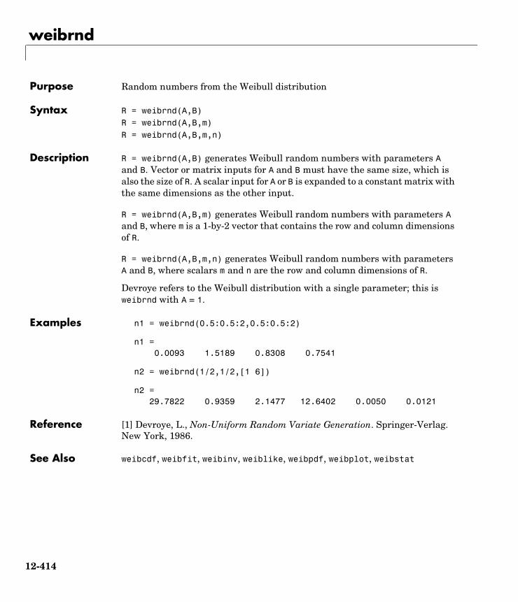
weibrnd
12weibrndPurpose Random numbers from the Weibull distribution
Syntax R = weibrnd(A,B)R = weibrnd(A,B,m)R = weibrnd(A,B,m,n)
Description R = weibrnd(A,B) generates Weibull random numbers with parameters A and B. Vector or matrix inputs for A and B must have the same size, which is also the size of R. A scalar input for A or B is expanded to a constant matrix with the same dimensions as the other input.
R = weibrnd(A,B,m) generates Weibull random numbers with parameters A and B, where m is a 1-by-2 vector that contains the row and column dimensions of R.
R = weibrnd(A,B,m,n) generates Weibull random numbers with parameters A and B, where scalars m and n are the row and column dimensions of R.
Devroye refers to the Weibull distribution with a single parameter; this is weibrnd with A = 1.
Examples n1 = weibrnd(0.5:0.5:2,0.5:0.5:2)
n1 = 0.0093 1.5189 0.8308 0.7541
n2 = weibrnd(1/2,1/2,[1 6])
n2 = 29.7822 0.9359 2.1477 12.6402 0.0050 0.0121
Reference [1] Devroye, L., Non-Uniform Random Variate Generation. Springer-Verlag. New York, 1986.
See Also weibcdf, weibfit, weibinv, weiblike, weibpdf, weibplot, weibstat
12-414

weibstat
12weibstatPurpose Mean and variance for the Weibull distribution
Syntax [M,V] = weibstat(A,B)
Description [M,V] = weibstat(A,B) returns the mean and variance for the Weibull distribution with parameters specified by A and B. Vector or matrix inputs for A and B must have the same size, which is also the size of M and V. A scalar input for A or B is expanded to a constant matrix with the same dimensions as the other input.
The mean of the Weibull distribution with parameters a and b is
and the variance is
Examples [m,v] = weibstat(1:4,1:4)
m = 1.0000 0.6267 0.6192 0.6409
v = 1.0000 0.1073 0.0506 0.0323
weibstat(0.5,0.7)
ans =
3.4073
See Also weibcdf, weibfit, weibinv, weiblike, weibpdf, weibplot, weibrnd
a
1b---–
Γ 1 b 1–+( )
a
2b---–
Γ 1 2b 1–+( ) Γ2 1 b 1–
+( )–
12-415

wishrnd
12wishrndPurpose Generate Wishart random matrix
Syntax W = wishrnd(SIGMA,df)W = wishrnd(SIGMA,df,D)[W,D] = wishrnd(SIGMA,df)
Description W = wishrnd(SIGMA,df) generates a random matrix W having the Wishart distribution with covariance matrix SIGMA and with df degrees of freedom.
W = wishrnd(SIGMA,df,D) expects D to be the Cholesky factor of SIGMA. If you call wishrnd multiple times using the same value of SIGMA, it's more efficient to supply D instead of computing it each time.
[W,D] = wishrnd(SIGMA,df) returns D so you can provide it as input in future calls to wishrnd.
See Also iwishrnd
12-416

x2fx
12x2fxPurpose Transform a factor settings matrix to a design matrix
Syntax D = x2fx(X)D = x2fx(X,'model')
Description D = x2fx(X) transforms a matrix of system inputs, X, to a design matrix for a linear additive model with a constant term.
D = x2fx(X,'model') allows control of the order of the regression model. 'model' can be one of these strings:
Alternatively model can be a matrix of terms. In this case, each row of model represents one term. The value in a column is the exponent to which the same column in X for that term is raised, D(i,j) = prod(x(i,:).^model(j,:)). This allows for models with polynomial terms of arbitrary order.
The order of columns for a quadratic model is:
1 Constant term
2 Linear terms (the input X columns 1,2,...,k)
3 Interaction terms formed by taking pairwise products of X columns (1,2), (1,3), ..., (1,k), (2,3), ..., (k-1,k)
4 Squared terms in the order 1,2,...,k
Other models use a subset of these terms but keep them in this order.
x2fx is a utility function for rstool, regstats, and cordexch.
Examples Example 1.
x = [1 2 3]'; model = [0 1 2]';D = x2fx(x,model)
D =
'interaction' Includes constant, linear, and cross product terms
'quadratic' Includes interactions and squared terms
'purequadratic' Includes constant, linear, and squared terms
12-417

x2fx
1 1 1 1 2 4 1 3 9
The first column is x to the 0th power. The second column is x to the 1st power. And the last column is x squared.
Example 2.
x = [1 2 3;4 5 6]'; model = 'quadratic';D = x2fx(x,model)
D =
1 1 4 4 1 16 1 2 5 10 4 25 1 3 6 18 9 36
Let x1 be the first column of x and x2 be the second. Then the first column of D is the constant term, the second column is x1, the third column is x2, the fourth column is x1x2, the fifth column is x1
2, and the last columns is x22.
See Also rstool, candexch, candgen, cordexch, rowexch, regstats
12-418

xbarplot
12xbarplotPurpose X-bar chart for Statistical Process Control
Syntax xbarplot(DATA)xbarplot(DATA,conf)xbarplot(DATA,conf,specs,'sigmaest')[outlier,h] = xbarplot(...)
Description xbarplot(DATA) displays an x-bar chart of the grouped responses in DATA. The rows of DATA contain replicate observations taken at a given time, and must be in time order. The graph contains the sample mean for each group, a center line at the average value, and upper and lower control limits. The limits are placed at a three-sigma distance on either side of the center line, where sigma is an estimate of the standard deviation of . If the process is in control, fewer than 3 out of 1000 observations would be expected to fall outside the control limits by random chance. So if you observe points outside the limits, you can take this as evidence that the process is not in control.
xbarplot(DATA,conf) allows control of the confidence level of the upper and lower plotted confidence limits. The default conf = 0.9973 produces three-sigma limits.
norminv(1 - (1-.9973)/2)
ans = 3
To get k-sigma limits, use the expression 1-2*(1-normcdf(k)). For example, the correct conf value for 2-sigma limits is 0.9545, as shown below.
k = 2;1-2*(1-normcdf(k))
ans = 0.9545
xbarplot(DATA,conf,specs) plots the specification limits in the two element vector specs.
xbarplot(DATA,conf,specs,'sigmaest') specifies how xbarplot should estimate the standard deviation. Acceptable values are:
xx
x
12-419

xbarplot
• 's' – use the average of the group standard deviations (default)
• 'v' – use the square root of a pooled variance estimate
• 'r' – use the average range with each group; requires 25 or fewer observations per group
[outlier,h] = xbarplot(DATA,conf,specs) returns outlier, a vector of indices to the rows where the mean of DATA is out of control, and h, a vector of handles to the plotted lines.
Example Plot an x-bar chart of measurements on newly machined parts, taken at one hour intervals for 36 hours. Each row of the runout matrix contains the measurements for four parts chosen at random. The values indicate, in thousandths of an inch, the amount the part radius differs from the target radius.
load partsxbarplot(runout,0.999,[-0.5 0.5])
The points in groups 21 and 25 are out of control, so the mean in those groups was higher than would be expected by random chance alone. There is evidence that the process was not in control when those measurements were collected.
See Also capaplot, histfit, ewmaplot, schart
0 5 10 15 20 25 30 35 40−0.5
−0.4
−0.3
−0.2
−0.1
0
0.1
0.2
0.3
0.4
0.5
21 25
UCL
LCL
CL
Xbar ChartUSL
LSL
Samples
Mea
sure
men
ts
12-420

zscore
12zscorePurpose Standardized Z score
Syntax Z = zscore(D)
Description Z = zscore(D) returns the deviation of each column of D from its mean, normalized by its standard deviation. This is known as the Z score of D.
For column vector V, the Z score is Z = (V-mean(V))./std(V).
12-421

ztest
12ztestPurpose Hypothesis testing for the mean of one sample with known variance
Syntax h = ztest(x,m,sigma)h = ztest(x,m,sigma,alpha)[h,sig,ci,zval] = ztest(x,m,sigma,alpha,tail)
Description h = ztest(x,m,sigma) performs a Z test at significance level 0.05 to determine whether a sample x from a normal distribution with standard deviation sigma could have mean m.
h = ztest(x,m,sigma,alpha) gives control of the significance level alpha. For example, if alpha = 0.01 and the result is h = 1, you can reject the null hypothesis at the significance level 0.01. If h = 0, you cannot reject the null hypothesis at the alpha level of significance.
[h,sig,ci] = ztest(x,m,sigma,alpha,tail) allows specification of one- or two-tailed tests, where tail is a flag that specifies one of three alternative hypotheses:
• tail = 0 specifies the alternative (default)
• tail = 1 specifies the alternative
• tail = -1 specifies the alternative
zval is the value of the Z statistic
where is the number of observations in the sample.
sig is the probability that the observed value of Z could be as large or larger by chance under the null hypothesis that the mean of x is equal to m.
ci is a 1-alpha confidence interval for the true mean.
Example This example generates 100 normal random numbers with theoretical mean zero and standard deviation one. The observed mean and standard deviation are different from their theoretical values, of course. We test the hypothesis that there is no true difference.
x = normrnd(0,1,100,1);
x m≠x m>x m<
z x m–
σ n⁄---------------=
n
12-422

ztest
m = mean(x)m = 0.0727
[h,sig,ci] = ztest(x,0,1)
h = 0
sig = 0.4669
ci = -0.1232 0.2687
The result, h = 0, means that we cannot reject the null hypothesis. The significance level is 0.4669, which means that by chance we would have observed values of Z more extreme than the one in this example in 47 of 100 similar experiments. A 95% confidence interval on the mean is [-0.1232 0.2687], which includes the theoretical (and hypothesized) mean of zero.
12-423

ztest
12-424

A
Selected Bibliography

A Selected Bibliography
A-2
[1] Atkinson, A.C., and A.N. Donev, Optimum Experimental Designs, Oxford Science Publications 1992.
[2] Bates, D. and D. Watts. Nonlinear Regression Analysis and Its Applications, John Wiley and Sons. 1988. pp. 271–272.
[3] Bernoulli, J., Ars Conjectandi, Basiliea: Thurnisius [11.19], 1713
[4] Box, G.E.P. and N.R. Draper, Empirical Model-Building and Response Surfaces, Wiley, New York. 1987.
[5] Box, G.E.P., W.G. Hunter, and J.S. Hunter. Statistics for Experimenters. Wiley, New York. 1978.
[6] Chatterjee, S. and A.S. Hadi. Influential Observations, High Leverage Points, and Outliers in Linear Regression. Statistical Science, 1986. pp. 379–416.
[7] Dobson, A. J., An Introduction to Generalized Linear Models, 1990, CRC Press.
[8] Efron, B., and R.J. Tibshirani. An Introduction to the Bootstrap, Chapman and Hall, New York. 1993.
[9] Evans, M., N. Hastings, and B. Peacock. Statistical Distributions, Second Edition. John Wiley and Sons, 1993.
[10] Hald, A., Statistical Theory with Engineering Applications, John Wiley and Sons, 1960. p. 647.
[11] Hogg, R.V., and J. Ledolter. Engineering Statistics. MacMillan Publishing Company, 1987.
[12] Johnson, N., and S. Kotz. Distributions in Statistics: Continuous Univariate Distributions. John Wiley and Sons, 1970.
[13] McCullagh, P., and J. A. Nelder, Generalized Linear Models, 2nd edition, 1990, Chapman and Hall.
[14] Montgomery, D.C., Design and Analysis of Experiments, Wiley, New York. 1984.
[15] Moore, J., Total Biochemical Oxygen Demand of Dairy Manures. Ph.D. thesis. University of Minnesota, Department of Agricultural Engineering, 1975.

[16] Poisson, S.D., Recherches sur la Probabilité des Jugements en Matiere Criminelle et en Metière Civile, Précédées des Regles Générales du Calcul des Probabilitiés. Paris: Bachelier, Imprimeur-Libraire pour les Mathematiques, 1837.
[17] “Student,” On the Probable Error of the Mean. Biometrika, 6:1908. pp. 1-25.
[18] Weibull, W., A Statistical Theory of the Strength of Materials. Ingeniors Vetenskaps Akademiens Handlingar, Royal Swedish Institute for Engineering Research. Stockholm, Sweden, No. 153. 1939.
A-3

A Selected Bibliography
A-4

Index
Aabsolute deviation 3-5additive effects 4-9alternative hypothesis 6-3analysis of variance 2-23
multivariate 7-20N-way 4-12one-way 4-4two-way 4-9
ANOVA 4-2anova1 12-19anova2 12-25anovan 12-29aoctool 12-35aoctool demo 11-10average linkage 12-219
Bbacteria counts 4-4barttest 12-38baseball odds 12-48, 12-50bbdesign 12-39Bera-Jarque. See Jarque-BeraBernoulli random variables 12-52beta distribution 2-11betacdf 12-40betafit 12-41betainv 12-43betalike 12-44betapdf 12-45betarnd 12-46betastat 12-47binocdf 12-48binofit 12-49binoinv 12-50binomial distribution 2-13
negative. See also negative binomial distribuiton
binopdf 12-51binornd 12-52binostat 12-53bootstrap 12-54bootstrap sampling 3-19box plots 8-3Box-Behnken designs 10-9
generating 12-39boxplot 12-56
Ccandexch 12-59candgen 12-61canoncorr 12-62capability studies 9-6capable 12-64capaplot 12-66casenames
reading from file 12-68writing to file 12-69
caseread 12-68casewrite 12-69ccdesign 12-70cdf
definition 2-5cdf 12-72cdfplot 12-73central composite designs 10-8
generating 12-70Central Limit Theorem 2-34centroid linkage 12-219Chatterjee and Hadi example 4-20chi2cdf 12-75
I-1

Index
I-2
chi2inv 12-76chi2pdf 12-77chi2rnd 12-78chi2stat 12-79chi-square distributions 2-16circuit boards 12-51City Block metric
in cluster analysis 12-304classical multidimensional scaling 7-47
cmdscale function 12-86overview 7-47reconstructing a map 7-49simple example 7-48
classification trees 5-8See also decision trees
classify 12-80cluster 12-82cluster analysis 7-26
functions 12-13hierarchical clustering 7-26K-means clustering 7-40
cluster tree creation 12-218from data 12-84from linkage output 12-82
cluster treesinconsistency coefficient 12-188plotting 12-106
clusterdata 12-84cmdscale 12-86coin 12-155combnk 12-88comparisons, multiple 4-6complete linkage 12-219confidence intervals
hypothesis tests 6-3nonlinear regression 5-6
control charts 9-3
EWMA charts 9-5S charts 9-4Xbar charts 9-3
cophenet 12-89cophenetic correlation coefficient 12-89
defined 7-32cordexch 12-91corr 12-93corrcoef 12-95correlation coefficients 12-93, 12-95cov 12-98Cp index 9-6, 12-64Cpk index 9-6, 12-64crosstab 12-99cumulative distribution
functions 12-5cumulative distribution function (cdf) 2-5
empirical 3-16graphing an estimate 8-8
Ddata partitioning
K-means clustering 7-40data sets
statistical examples 12-16daugment 12-101dcovary 12-103decision trees 5-8
computing error rate 12-383computing response values 12-386creating 12-377creating subtrees 12-380displaying 12-375example 5-8fitting 12-377pruning 12-380

Index
demos 11-1, 12-16design of experiments 11-19polynomial curve fitting 11-5probability distributions 11-3random number generation 11-18
dendrogram 12-106, 12-234density estimation
ksdensity function 12-202descriptive statistics 3-1
functions 12-9Design of Experiments
functions 12-13design of experiments 10-1
Box-Behnken designs 10-9central composite designs 10-8D-optimal designs 10-11fractional factorial designs 10-6full factorial designs 10-4response surface designs 10-8
dimension reductioncommon factor analysis 12-122PCA from covariance matrix 12-299PCA from raw data matrix 12-319PCA residuals 12-300
discrete uniform distribution 2-19dissimilarity matrix
creating 7-27distance matrix
creating 7-27distribution testing
functions 12-15distributions 2-1
supported 2-11disttool 12-109disttool demo 11-3DOE. See Design of ExperimentsD-optimal designs 10-11
creating from candidate set 12-59generating candidate set 12-61
dummyvar 12-110
Eecdf 12-111empirical cumulative distribution function 3-16
ecdf function 12-111erf 2-34error function 2-34errorbar 12-113estimate 11-6Euclidean distance
in cluster analysis 12-303EWMA charts 9-5ewmaplot 12-114expcdf 12-116expfit 12-117expinv 12-118exponential distribution 2-20exppdf 12-119exprnd 12-120expstat 12-121extrapolated 12-322
FF distributions 2-22F statistic 4-21factor analysis
maximum likelihood 12-122factoran 12-122factorial designs
fractional 10-6full 10-4generating fractional 12-135
I-3

Index
I-4
factorial designs (continued)generating full 12-147
fcdf 12-131ff2n 12-132file I/O functions 12-16finv 12-133floppy disks 12-182fpdf 12-134fracfact 12-135fractional factorial designs 10-6
generating 12-135friedman 12-139Friedman’s test 4-34frnd 12-143fstat 12-144fsurfht 12-145full factorial designs 10-4
generating 12-147fullfact 12-147furthest neighbor linkage 12-219
Ggamcdf 12-148gamfit 12-149gaminv 12-150gamlike 12-151gamma distribution 2-25gampdf 12-152gamrnd 12-153gamstat 12-154Gaussian 12-179geocdf 12-155geoinv 12-156geomean 12-157geometric distribution 2-27geopdf 12-158
geornd 12-159geostat 12-160gline 12-161glmdemo 12-162glmdemo demo 11-21glmfit 12-163glmval 12-168gname 12-170gplotmatrix 12-172group mean clusters, plot 7-25grouped plot matrix 7-20grpstats 12-175gscatter 12-176Guinness beer 2-39, 12-370
Hharmmean 12-178hat matrix 4-19hierarchical clustering 7-26
basic procedure 7-27computing inconsistency coefficient 12-188creating cluster tree 12-218creating clusters 7-37creating clusters from data 12-84creating clusters from linkage output 12-82depth of comparison 7-33determining proximity 12-302evaluating cluster formation 12-89finding dissimilarities betwen objects 7-33finding similarities beween objects 7-27formatting distance information 12-362grouping objects 7-30inconsistency coefficient 12-188plotting cluster trees 12-106
hierarchiical clusteringcophenetic correlation coefficient 12-89

Index
hist 12-179histfit 12-180histogram 11-18Hotelling’s T squared 7-12hougen 12-181Hougen-Watson model 5-3hygecdf 12-182hygeinv 12-183hygepdf 12-184hygernd 12-185hygestat 12-186hypergeometric distribution 2-28hypotheses 2-23hypothesis tests 6-1
functions 12-15
Iicdf 12-187incomplete beta function 2-11incomplete gamma function 2-25inconsistency coefficient 12-188inconsistent 12-188inspector 12-307interaction 4-9interpolated 12-365interquartile range (iqr) 3-5inverse cdf 2-5inverse cumulative distribution
functions 12-6iqr 12-190iwishrnd 12-191
JJarque-Bera test 12-192jbtest 12-192
KKaplan-Meier cumulative distribution function
12-111kernel bandwidth 3-13kernel smoothing function 3-15K-means clustering 7-40
cluster separation 7-41creating clusters 12-194example 7-41local minima 7-45number of clusters 7-43overview 7-40silhouette plot 12-358
kmeansdata partitioningK-means clustering 12-194
kruskalwallis 12-198Kruskal-Wallis test 4-34ksdensity 12-202kstest 12-204kstest2 12-208kurtosis 12-211
Llatin hypercube sample 12-214
normal distribution 12-215least squares 12-315leverage 12-213lhsdesign 12-214lhsnorm 12-215light bulbs, life of 12-118likelihood function 12-45Lilliefors test 6-5lillietest 12-216linear models 4-1
functions 12-11generalized 4-28
I-5

Index
I-6
linear transformationProcrustes 12-320
linkage 12-218logncdf 12-221logninv 12-222lognormal distribution 2-29lognpdf 12-224lognrnd 12-225lognstat 12-226lottery 12-398lsline 12-227LU factorizations 12-314
Mmad 12-228mahal 12-229Mahalanobis distance 12-229
in cluster analysis 12-303MANOVA 7-20manova1 12-230manovacluster 12-234maximum likelihood
factor analysis 12-122MDS
See also multidimensional scalingmean 2-9
of probability distribution 2-9mean 12-236Mean Squares (MS) 12-19measures of
central tendency 3-3dispersion 3-5
median 12-237metric multidimensional scaling
See also classical multidimensional scalingMinkowski metric
in cluster analysis 12-304mle 12-238models
linear 4-1nonlinear 5-1
moment 12-239moments of distribution
functions 12-8Monte Carlo simulation 12-190multcompare 12-240multidimensional arrays
classical (metric) scaling 12-86multidimensional scaling (MDS)
classical (metric) 7-47multiple linear regression 4-18multivariate analysis of variance 7-20
example 7-20multivariate statistics 7-1
analysis of variance 7-20cluster analysis 7-26functions 12-13hierarchical clustering 7-26K-means clustering 7-40Principal Components Analysis 7-3
mvnpdf 12-247mvnrnd 12-248mvtrnd 12-249
Nnanmax 12-250nanmean 12-251nanmedian 12-252nanmin 12-253NaNs 3-7nanstd 12-254nansum 12-255

Index
nbincdf 12-256nbinfit 12-258nbininv 12-259nbinpdf 12-260nbinrnd 12-262nbinstat 12-263ncfcdf 12-265ncfinv 12-267ncfpdf 12-268ncfrnd 12-269ncfstat 12-270nctcdf 12-271nctinv 12-272nctpdf 12-273nctrnd 12-274nctstat 12-275ncx2cdf 12-276ncx2inv 12-278ncx2pdf 12-279ncx2rnd 12-280ncx2stat 12-281nearest neighbor linkage 12-219negative binomial distribution 2-31
confidence intervals 12-258cumulative distribution function (cdf) 12-256definition 2-31inverse cumulative distribution function (cdf)
12-259mean and variance 12-263modeling number of auto accidents 2-32nbincdf function 12-256nbininv function 12-259nbinpdf function 12-260parameter estimates 12-258probability density function (pdf) 12-260random matrices 12-262
Newton’s method 12-150
nlinfit 12-282nlintool 12-284nlintool demo 5-7nlparci 12-285nlpredci 12-286noncentral F distribution 2-23nonlinear regression
functions 12-12nonlinear regression models 5-1nonparametric testing
functions 12-15normal distribution 2-34normal probability plots 8-2, 8-4normalizing a dataset 7-28
using zscore 12-421normcdf 12-288normdemo 12-296normfit 12-289norminv 12-290normlike 12-291normpdf 12-292normplot 12-293normrnd 12-295normstat 12-297notation, mathematical conventions 1-6notches 12-56null 6-3null hypothesis 6-3
Oone-way analysis of variance (ANOVA) 4-2outliers 3-3
I-7

Index
I-8
Pparameter estimation
functions 12-4pareto 12-298Pascal, Blaise 2-14PCA. See Principal Components Analysispcacov 12-299pcares 12-300pdf
definition 2-4pdf 12-301pdist 12-302percentiles 3-11perms 12-306plots 3-11plotting
statistical functions 12-10poisscdf 12-307poissfit 12-309poissinv 12-310Poisson distribution 2-36poisspdf 12-311poissrnd 12-312poisstat 12-313polyconf 12-314polyfit 12-315polynomial 11-5polytool 12-316polytool demo 11-5polyval 12-317popcorn 12-27, 12-141prctile 12-318Principal Components Analysis (PCA) 7-3
component scores 7-7component variances 7-10Hotelling’s T squared 7-12principal components 7-7
quality of life example 7-4Scree plot 7-11
princomp 12-319probability density
functions 12-5probability density estimation 3-13
comparing estimates 3-16function 12-202kernel bandwidth 3-13kernel smoothing functioon 3-15
probability density function (pdf)definition 2-4
probability distributionmean and variance 2-9
probability distributions 2-1functions 12-4
process controlstatistical 9-1
procrustes 12-320Procrustes Analysis 12-320p-value 4-11, 6-3
Qqqplot 12-322QR decomposition 4-18quality assurance 12-51quantile-quantile plots 8-2, 8-6
Rrandom 12-324random number generation 2-7
direct 2-7functions 12-7inverted 2-7rejection 2-8

Index
random numbers 2-7random samples
inverse Wishart 12-191latin hypercube 12-214latin hypercube with normal distribution
12-215Wishart 12-416
randtool 12-325randtool demo 11-18range 12-326ranksum 12-327raylcdf 12-328raylinv 12-329raylpdf 12-330raylrnd 12-331raylstat 12-332rcoplot 12-333reconstruction
map from inter-city distances 7-49refcurve 12-334reference lines 11-3references A-1refline 12-335regress 12-336regression 2-23
nonlinear 5-1robust 4-32stepwise 4-24
regression trees 5-8See also decision trees
regstats 12-338relative efficiency 12-190residuals 4-21response surface designs 10-8Response Surface Methodology (RSM) 4-22respoonse surface designs
Box-Behnken 10-9
central composite 10-8ridge 12-341robust 3-3robust linear fit 12-322robustdemo 12-343robustdemo demo 11-22robustfit 12-344rowexch 12-348rsmdemo 12-350rsmdemo demo 11-19R-square 4-21rstool 12-351rstool demo 4-22
SS charts 9-4scaling arrays
classical multidimensional 12-86scatter plots 8-10
grouped 7-20schart 12-352Scree plot 7-11segmentation analysis 7-26significance level 6-3signrank 12-354signtest 12-356silhouette 12-358similarity matrix
creating 7-27simulation 12-190single linkage 12-219skewness 8-3skewness 12-360squareform 12-362standard normal 12-292
I-9

Index
I-10
Standardized Euclidean distancein cluster analysis 12-303
statistical plots 8-1Statistical Process Control 9-1
capability studies 9-6control charts 9-3functions 12-11
statistical references A-1statistically significant 12-19, 12-198, 12-230stepwise 4-24, 12-364stepwise regression 4-24Sum of Squares (SS) 12-19surfht 12-365symmetric 12-148
Tt distributions 2-39
noncentral 2-40tab-delimited data
reading from file 12-371tabular data
reading from file 12-367tabulate 12-366taxonomy analysis 7-26tblread 12-367tblwrite 12-369tcdf 12-370tdfread 12-371tinv 12-373tpdf 12-374treefit 12-377treeprune 12-380trees
See also decision treesSee also decision trees
treeshow 12-375
treetest 12-383treeval 12-386trimmean 12-388trnd 12-389tstat 12-390ttest 12-391ttest2 12-393two-way ANOVA 4-9typographical conventions (table) xiv
Uunbiased 12-363, 12-406unidcdf 12-395unidinv 12-396unidpdf 12-397unidrnd 12-398unidstat 12-399unifcdf 12-400unifinv 12-401unifit 12-402uniform distribution 2-42unifpdf 12-403unifrnd 12-404unifstat 12-405
Vvar 12-406variance 2-9
of probability distribution 2-9
Wward linkage 12-220weibcdf 12-408weibfit 12-409

Index
weibinv 12-410weiblike 12-411weibpdf 12-412weibplot 12-413weibrnd 12-414weibstat 12-415Weibull distribution 2-43Weibull probability plots 8-7Weibull, Waloddi 2-43whiskers 8-3, 12-56Wishart random matrix 12-416
inverse 12-191wishrnd 12-416
Xx2fx 12-417Xbar charts 9-3xbarplot 12-419
Zzscore 12-421ztest 12-422
I-11

Index
I-12