unlimited - apps.dtic.mil

UNLIMITED

RSRE

MEMORANDUM No. 4148

ROVAL SIGNALS & RADARESTABLISHMENT

RADIAL BASIS FU NCTIONS, MULTI-VARIABLEFUNCTIONAL INTERPOLATION AND ADAPTIVE NETWORKS

Auithors: D S Broomnhead and D Lowe

.DTICSELECTE

PROCUREMENT EXECUTIVE,

6 MINISTRY OF DEFENCE,7- RAS RE MALVERN,

WORCS.

QDiSTAIBI)TTON STATEMENT AATProved for public, releae

0 Piat *bttioin Uaivmited

UNL-IMITED

Royal Signals and Radar Establishment

Memorandum 4148

Radial Basis Functions,Multi-Variable Functional Interpolation

and

Adaptive Nctworks.

D.S. Broomhead 'Royal Signals and Radar Establishment

St. Andrews Road, Great Malvern, Worcs. WRI4 3PS. United Kingdom

David Lowe b

Speech Research Unit, Royal Signals and Radar Establishment

St. Andrews Road, Great Maivern, Worcs. WR14 3PS. United Kingdom

March 28, 1988

Abstract

The relationship between 'learning' in adaptive layered networks and the fitting ofdata with high dimensional surfaces is discussed. This leads naturally to a pictureof 'generalisation' in terms of interpolation between known data points and suggestsa rational approach to the theory of such networks. A class of adaptive networks isidentified which makes the interpolation scheme explicit. This class has the propertythat learning is equivalent to the solution of a set of linear equations. These networksthus represent nonlinear relationships while having a guaranteed learning rule.

"Electronic Mail address from USA: dob%rare. mod. uklrelay. mod. ukElectronic Mail address from the UK: dsb',rore -mod. uk~uk. ac. ucl. cs.nss

'Electronic Mail address from USA. dl%rsre. mod. uktrelay. mod. ukElectronic Mail address from the UK: d1%rsre .mod.uk~uk. ac .uci. cm .n88

Copyright @ Controller HMSO, London, 1988.

Multi- Variable Functional Interpolation and Adaptive Networks

Contents

1 Introduction 1

2 Multi-variable functional Interpolationusing radial basis functions 2

3 The radial basis function methodviewed as a layered network 5

4 Specific example (i):the exclusive-OR Problem and an exact solution. 8

5 An analytic solution to a non-exact problem:The exclusive-OR problem with two centres. 13

5.1 The approximate exclusive-OR without an output bias ................ 13

5.2 The approximate exclusive-OR including an output bias .............. 16

6 Numerical examples:the prediction of chaotic time series. 19

7 Conclusion 24

A Solving linear inverse problems. 26

B An analytic solution of the exact n-bit parity problem 28

C The quadratic and doubling maps 31

Acceol ror70

NTIS CRA&IDIIC TAB 2l

By

Avealabiity Codie

Avaii I ®D~ist .o :a,-I01710.i

° .. . .. . . ... . [ . .N.. . . . . . .

D.S. Broomhead and David Lowe

List of Figures

1 A schematic diagram of the feed-forward layered network model representedby the radial basis function expansion ..... ...................... 6

2 The exclusive-OR solution (i). Obtained using a Euclidean distance functionand Gaussian radial basis functions centred at the corners of the unit square. 11

3 The exclusive-OR solution (ii). Obtained using a Euclidean distance functionand multiquadric radial basis functions centred at the corners of the unitsquare ........... ....................................... 11

4 Equivalent network for exclusive-OR with A2 set to zero .............. 12

5 Equivalent network for exclusive-OR with A, set to zero .............. 12

6 Contours of the approximate exclusive-OR solution, without an output bias. 14

7 Contours of the approximate exclusive-OR solution, including an outputbias .......... .......................................... 17

8 The Quadratic Map: A figure showing the actual (solid line), and predicted(filled squares) outputs of the network over the interval 10, 1] for one iterate. 20

9 The Doubling Map: A figure showing the actual (solid line), and predicted(filled squares) outputs of the network over the interval 10, 11 for one timestep into the future for the doubling map ...... .................... 21

10 The Quadratic Map: The log normalised error showing the training (solidcircles) and recognition data (open circles) as a function of the number ofradial basis function centres. Euclidean norm and a Gaussian radial basisfunction (0 = exp[-z 2 n2/16j) were used ............................ 22

11 The Doubling Map: The log normalised error showing the training (solidcircles) and recognition data (open circles) as a function of the number ofradial basis function centres. Euclidean norm and a Gaussian radial basisfunction (0 = exp[-z 2n2/16]) were used ............................ 23

12 The hypercube of the 3-bit parity problem ...... .................. 29

List of Tables

1 Symbolic mapping of the exclusive-OR problem .................... 8

2 The character table for C4 . . . . . . . . . . . . . . . . . . . . . . . . . . . .. . . . . 27

3 Symbolic mapping of the n-bit parity problem for the case n = 3 ....... ... 28

-11-

Multi-Variable Functional Interpolation and Adaptive Networks

1 Introduction

The strong resurgence of interest in 'self-learning machines', whose ancestors include theperceptrons of the 1960's, is at least partly driven by the expectation that they will provide anew source of algorithms/architectures for the processing of complex data. This expectationis based on an analogy with connectionist models of animal brains. The brain is able to copewith sophisticated recognition and inductive tasks far beyond the capabilities of systemsbased on present computing logic and architectures.

An example of an everyday task for the human brain which illustrates this point, isthe recognition of humain speech. For automatic speech recognition one wishes to deduceproperties (the implied message) from the statistics of a finite input data set even thoughthe speech will be subject to nonlinear distortions due to noise, sex, age, health and accentof the speaker. This has proved to be notoriously difficult. Over the past decade, oneof the most successful techniques developed for speech recognition has been based aroundHidden Markov Models (see for instance [1,2,3]). In this scheme, speech is modelled as asequence of causal stationary stochastic processes determined by a finite number of allowablestates, state transitions, a matrix of stationary transition probabilities and an initial statedistribution. There is, in addition, a learning algorithm (Baum-Welch iteration) to finetune the parameters of the model which increases the likelihood that each model producesit's associated data. However, one of the problems with this approach involves the a prioriassumptions made regarding the topology of the Hidden Markov model (number of states,allowable transitions etc). As long as the total possible input data is consistent with theassumptions made in the original model, then one can expect a faithful representationof the data. This unfortunately presupposes that we already know how to model speechadequately.

In an attempt to circumvent this problem, self-learning machines have been employed.The virtue of these is that no explicit model of speech is required. For instance, the multi-layer perceptron (which is a layered nonlinear network) embodies a set of nonlinear, 'hidden'units whose task is to encode the higher order constraints of the input data [41. This isachieved by varying weights governing the strengths of connections between the units inorder to minimise the error in relating known input-output pairs (the 'training' set). Thisprocess has become known as "learning". The ability of the network to give subsequentlyreasonable (in some sense) outputs for inputs not contained in the training set is termed"generalisation". In effect a multi-layer perceptron of given geometry with given nonlinearresponses of the units constitutes an M-parameter family of models (where M is the totalnumber of weights which are varied). It is currently an act of faith, based on encouragingpractical results, that such families are broad enough to include models of speech which areadequate for the purposes of classification. This means, however, that the design of a multi-layer perceptron for a specific task remains an empirical art. In particular, how many hiddenunits should be employed and in what configuration, how much training data is needed,and what initial inter-connection strengths ha-, to be as-tigned? Sume experiiientai workhas been performed which addresses these problems (for instance [5,6]) although it is fair tocomment that an understanding of these issues is still lacking. The source of the difficultyis the implicit relationship between these externally controllable factors, and the modelultimately represented by the network.

The present paper investigates the implicit assumptions made when employing a feed-forward layered network model to analyse complex data. The approach will be to view such

-1-


a network as representing a map from an n-dimensional input space to an n'-dimensionaloutput space, say a : R n , Rn'. This map will be thought of as a graph r c Rn x ln' (in thesame way that a : !t -+ IR, where s(z) = x may be thought of as a parabola drawn in IR2).From this point of view, "error free" training data presented to the network in the form ofinput-output pairs represent points on the graph, r and the learning phase of an adaptivenetwork constitutes the optimisation for a fitting procedure for r based on the knowndata points. Generalisatibn is therefore synonymous with interpolation between the datapoints with the interpolation being along the constrained surface generated by the fittingprocedure as the optimum approximation to r. In this picture the implicit assumptionsmade when using a multi-layer perceptron concern the nature of the fitting procedure, andclearly relate directly to the way in which the network generalises. Thus, we are led to thetheory of multi-variable interpolation in high dimensional spaces. In subsequent sections,we shall exploit some of the mathematics of this expanding field of research to develop anew type of layered network model in which the nature of the fitting procedure is explicit.This class of layered network model will be shown to be of considerable interest in itself. Inaddition however, it is hoped that the explicit nature of the fitting procedure will allow usto develop a better understanding of the general properties of layered nonlinear networkswhich perform an equivalent function.

2 Multi-variable functional interpolationusing radial basis functions

This section introduces briefly the method of Radial Basis Functions, a technique for in-terpolating in a high dimensional space which has recently seen important developments.Further details may be obtained from the review article of Powell 17) and the importantcontribution of Micchelli [8].

In the cited references the radial basis function approach is applied to the strict inter-polation problem which may be summarised as follows:-Problem: Given a set of m distinct vectors (data points), {x; i 1,2,..., m} in R" andm real numbers {fi;i = 1,2,. .. ,m}, choose a function s : R - R which satisfies theinterpolation conditions

8(x,-) =-f, ; = 1, 2,. .. , m I

Note that the function, 8, is constrained to go through the known data points.

There are clearly many criteria one could impose which wou!d restrict the possiblefunctional form of s(;:) (see for instance 19]). The Radial Basis Function approach constructsa linear space which depends on the position relative to the known data points accordingto an arbitrary distance measure. Thus, a set of m arbitrary (generally nonlinear) 'basis'functions 0(I1x - 9jI) is introduced, where z E IRn and 11... 11 denotes a norm imposed onR" which is usually taken to be Euclidean. The vectors y, E R ,i = 1,2,...,m are thecentres of the basis functions and taken to be sample data points. In terms of these basisfunctions, we consider interpolating functions of the form:-

inn()= A(1Z -v. ~E H (2)2=I

-2-


Inserting the interpolation conditions, equation (1) into equation (2), gives the followingset of linear equations for the coefficients {Aj),

= i :(3)(fm) = (A, A m) ( A)

whereA,, (Il-.u j) x, -= 1,2,.. .,m (4)

Given the existence of the inverse to matrix A with elements Aj, equation (3) uniquelydefines the coefficients Ai through A = A-'f.

In general, one might expect that for an arbitrary choice of 0 the matrix A could besingular. However, the results of Micchelli prove that for all positive integers m, n and fora large class of functions 0, the matrix A is non-singular if the data points are all distinct .

This discussion readily generalises to maps s : Rn - R n'. In this case the m distinctdata points in R n are associated with rn vectors L E Rn'. The interpolation condition ofequation (1) thus generalises to

Sk()= ,k s =k ,2,..., k= 1,2,...,n' (5)

which leads to interpolating functions of the form

m

si-(Z) ZA kA,(I1x- y x E IR kn (6)

The expansion coefficients Ajk are obtained using the inverse of the same matrix A definedin equation (4).

Once a suitable choice of the function 0 is made, and a convenient distance measure im-posed, the above relations exactly specify the interpolation problem which has a guaranteedsolution.

However, for certain classes of problem, the above analysis may not be a good strategyfor the following reason. A basic consideration when fitting data is the number of degrees offreedom required. That is, the minimum number of basis functions needed to generate anacceptable fit to the data. In the situation where the number of data points far exceeds thenumber of degrees of freedom there will be redundancy since we are constrained to use asmany radial basis functions as data points. In this case the strict interpolation conditionsgenerally result in this redundancy being used to fit misleadir:g variations due to imprecise,or noisy data.

It is possible to avoid this difficulty by weakening the interpolation conditions. Wesuggest the following generalisations to the conventional radial basis function approach.First, it may be necessary to distinguish between the data points, (X, i = 1, 2,..., m) andthe radial basis function centres, (y., j = 1,2,... ,no n0 < m) 1. The problem thusbecomes overspecified, the matrix A is not square, a unique inverse no longer exists, and theprevious exact problem becomes one of linear optimisation. In the following, we shall adopt

'in particular, we do not necessarily require that the radial basis function centres correspond to any of the .data points.

-3-

D.S. Brnomhead and David Lowe

a minimum norm least squares method by introducing the Moore-Penrose pseudo-inverse,A' of matrix A. For the case where rankA = no, this has the property that A+A= Iwhere I denotes the n0 x no identity matrix. The pseudo-inverse provides a unique solutionto the linear least squares problem [10] in the following sense,

Of all the vectors A which minimise the sum of squares IIAA - fl12 , the one which hasthe smallest norm (and hence minimises [JAll2) is given by A = A+L.

For this particular solution set, an expression may be derived for the normalised errorC, specifically,

N 1 lLf - (f)112

(7)

11 rm1= (AA+).,iL, - Li12

- N--S IfL - Q)112

where (f) is the mean value of the response vector over all the training data points. Notethat if the pseudo-inverse equals the exact inverse, then the left and right inverses are thesame and hence the matrix product AA+ is the m-dimensional identity matrix, and thiserror is zero.

An additional modification, which is useful particularly when f_(1) has a large x-independentcomponent, is to incorporate constant offsets {Aok} into the form of the interpolating func-tions

Sk(T) = \0k+ AikO(l[-1- y 11) xE En k = 1,2,...,n' (8)j=1

These coefficients enter the least squares formalism through an additional column in A

Ai 0 = 1 i= 1,2,...,m (9)

In this form, the radial basis function approach to multi-variable functional interpolationhas a close resemblance to adaptive network theory. This will be discussed in the followingsections. An important consequence of this approach which should be emphasised is thatthe determination of the nonlinear map (;) has been reduced to a problem in linear algebra.The coefficients Ajk appear linearly in the functional form of the mapping, therefore theproblem of determining the precise values, even in an overdetermined situation, has beenreduced to one of a linear least squares optimisation which has a 'guaranteed learningalgorithm' through the pseudo-inverse technique 2. Of course, this ,.eduction has assumedsuitable choices for the centres, {VI} and the function 0. It may be argued, therefore, that

the restriction of the optimisation by fixing these quantities is excessive and must limit therange of applicability of the approach. In the case of the strict interpolation this does notseem to be the case, at least as far as the choice of 0 is concerned [15]. There is evidence toshow (17], again for strict interpolation, that the effect of a suboptimal choice of the {Yj}is to reduce the rate of convergence of the expansion given in equation (6). For the leastsquares extensions described here, much less is known.

2AP a technical numerical point, the solution will not generally be obtained from the normal equations

(which may be ill-conditioned), but would be obtained via the efficient procedure of singular valueddecomposition.

-4-


3 The radial basis function methodviewed as a layered network

Much of the power and attraction of current adaptive network models is contained in thenonlinear aspects of the hidden units so that nonlinear input-output relationships may bemodelled. Unfortunately, since the error criterion, or cost function, depends on the responseof the nonlinear elements, the problem of finding a globally optimum solution becomes oneof unconstrained nonlinear least squares minimisation. Such problems can be solved usuallyonly by iterative techniques. For instance, 'error back-propagation' is a first order (onlydepends on the gradient of the function of interest) steepest descent technique which suffersfrom slow convergence properties due to it's tendency to zig-zag about the true direction toa minimum. More sophisticated iterative schemes derived from second order approximationshave been proposed which improve convergence properties (the quasi-Newton, or variablemetric algorithms-see for instance [111, Chapter 15 and [121). Recent works of note whichhave considered more general iterative strategies and found them to be orders of magnitudesuperior to back-propagation when applied to specific layered network problems are those ofLapedes and Farber [131 (conjugate gradients) and Watrous [141 (Davidon-Fletcher-Powelland Broyden-Fletceir-Goldfarb-Shanno). In spite of this effort, the difficulty remains thatthe solution obtained by such methods is not guaranteed to be the global optimum sincelocal minima may be found. There is no reason in the current iterative schemes why aleast squares minimisation solution obtained, will necessarily have the required form. Evenchoosing a good initial starting point for the iteration schemes will not necessarily implythat a good approximation to the global minimum will be obtained. It is important toknow how 'good' a solution is obtained by settling for a local minimum, and under whatconditions the solution at such a minimum has to be deemed unsatisfactory.

In the previous section it was shown that because of the linear dependence on the weightsin the radial basis function expansion, a globally optimum least squares interpolation ofnonlinear maps can be achieved. The relevance of this to layered network models is thatthe mapping produced by the radial basis function expression eqn. (6), has the form of aweighted sum over nonlinear functions. There is thus a natural correspondence with thefollowing general 3-layer network system, in which the layers are fully interconnected withadjacent layers, but there are no interconnections within the layers (see figure 1).

The input layer of this network model is a set of n-nodes waiting to accept the com-ponents of the n-dimensional vector z. These input nodes are directly connected to all ofthe hidden nodes. Associated with each connection is a scalar (yi, for the link betweenthe i-th input node and the j-th hidden node) such that the fan-in to a given node hasthe form of a hypersphere, i.e. in the case of a Euclidean r.orm, the input to the node is#j = Z2=x(z, - y,,) 2 where the zi are components of z. The 'hidden layer' consists of a setof no nodes, one for each radial basis function centre. The output of each of these is a scalar,generally nonlinear function of 6,. The hidden layer is fully connected to an output layercorresponding to the n'-components of the n'-dimensional response vector s(x) of the net-work. The input value received by each output unit is a weighted sum of all the outputs ofthe hidden units, where the strengths of connections from the j-th hidden unit to the k-thoutput unit are denoted by Ail. The response of each output unit is a linear function of itsnet input which may include the bias AOk. A natural extension is to allow for nonlinearity inthe response of the output units. Clearly, if the transfer function of these units is invertible,then it can be accounted for by a suitable modification of the interpolation conditions used

-5-


Input layer Hidden layer Output layer

2 3

Figure 1: A schematic diagram of the feed-forward layered network model represented bythe radial basis function expansion.

-6-


to derive the weights {Ajk}. This specifies, as a layered network model, the radial basisfunction expansion, equation (8), which produces a mapping from an n-dimensional inputspace to an n'-dimensional target space.

This type of network falls within the general class of nonlinear layered feedforwardnetworks. In particular we have specialised the geometry to a single hidden layer and fixedthe fan-in and fan-out to the hidden units as indicated. The choice of hyperspherical fan-in to the hidden units has the effect of sectioning the decision space into hypersphericalregions rather than hyperplanes which result from the more usual choice of a scalar producttype of fan-in. This has the advantage of allowing disjoint regions in the decision space,but which pertain to the same classification, to be satisfactorily resolved by the single'hidden' adaptive layer. Problems without simple connectivity would traditionally requiretwo hidden adaptive layers, as discussed in 1181, whereas the approach described in thispaper can deal with such problf ns by employing a single hidden layer.

In principle, the total set of adjustable parameters include the set of no-radial basisfunction centres, y.. as well as the set of (no + ) .n weights, .However, only the latter

are included in the least squares analysis in this paper in order to preserve the linearity ofthe learning procedure.

The radial basis function strategy may be applied to the general multi-layer perceptronfor which the output units have an invertible nonlinearity. Moreover, when extended toallow for variation in the input-hidden weights, this method provides an interesting pic-ture of learning. In particular, the hidden-output weights may be visualised as evolvingon a different 'time scale' to the input-hidden weights. Thus, as the input-hidden weightsevolve slowly by some nonlinear optimisation strategy, the hidden-output weights adjustthemselves rapidly through linear optimisation so as to always remain in the global mini-mum of an evolving error surface over the hidden-output weights which is parametricallycontrolled by the input-hidden weights.

The rest of this paper is concerned with various simple applications of the radial basisfunction network assuming a fixed set of centres. In the absence of any a priori knowledge,the centres, (y I} are either distributed uniformly within the region of IR' for which thereis data, or they are chosen to be a subset of the training points by analogy with strictinterpolation. We expect that with additional knowledge of the surface to be fitted, thefreedom to position the centres may be used to advantage to improve the convergence ofthe expansion (although not necessarily to improve the 'fit' to the unseen data). Evidencefor this as well as insight into the significance of the centres follows from the work ofPowell 115] who showed that for strict interpolation when n = n' = I and when 0(r) =r2k+I, (k = 0, 1,...), the radial basis function method is equivalent to interpolation withnatural splines. In this case the {y )} are the knots of the spline fit. Naturally, when thestrict interpolation is weakened to give a least squares interpolation, the significance of the'knots' in constraining the surface is also weakened. In what follows, we shall attempt tobe as general as possible in the analytic work by assuming an arbitrary form of 4. Wherenumerical work necessitates a specific choice, we have chosen to employ either a Gaussianform (O(r) _ exp[-r 2J) or a multiquadric (O(r) % v'+r2).

-7-


4 Specific example (i):the exclusive-OR Problem and an exact solution.

Input Number of 'ON' OutputPattern bits in input Pattern

00 -* 0 001 - 1 -. 110 - 1 -. 111 -. 2 0

Table 1: Symbolic mapping of the exclusive-OR problem.

The exclusive-OR problem defined by the symbolic mapping in Table 1 has been consideredinteresting because points which are closest (in terms of the Hamming distance) in the inputspace, map to regions which are maximally apart in the output space. This is a classicexample of a logic function that cannot be represented by a linear perceptron. Clearly, afunction which interpolates between the points given in Table 1 must oscillate, and may behard to represent using a subset of data points unless there is some built in symmetry inthe radial basis functions.

In what follows, we initially take one radial basis function centre determined by eachpiece of input data, so that both y, ,x are selections of the four ordered input patternsof Table 1. We choose to number the four possible input patterns as (0,0) - 1, (0, 1) -.2, (1,1) -- 3, (1,0) - 4 which we visualise to be the cyclically ordered corners of a square.The action of the network may be represented by

4

so that the set {A,) may be found from

4

A E A 00 1(--T - I*7II)j=1

ie.

For the ordering we have chosen, the vector L and the matrix A take the specific forms

(10)

and [ 4o €i 4y €A= 01 0 0 01 0v r21

01 0,/2 0'1 00o

ima, _ m m, mm mm o *i m)J

Multi-Variable Functional Interpolation and Adaptive Netwvnrks

where a labelling notation has been introduced so that 0 denotes the value ofp(II -_;izl),

01 denotes the value O(lx, - z,~,fl) and v/-2 represents O(lIx - -X±211), all counting being

performed cyclically around the square. Note that this is a labelling device and we will

not exploit the properties of any particular distance function at this stage (although the

notation Or, indicates that we have in mind a Euclidean metric as an example).

It will be convenient to construct A-' from the eigenvalue decomposition (see Ap-

pendix A for further details)

A VMVT

Since A is real symmetric, V is an orthogonal matrix with columns composed out of theorthogonal eigenvectors; in this case,

1 1 -1 0 _-VV = 2 1 1 - - (12)

1 -1 0 -=V'2

and p is the real, diagonal matrix

M A 0 0 0

0 PB 0 0

0 0 ME 00 ME

where

IA (Oo + 20, + v)

MB = (Oo - 20 + Ov-) (13)

ME = (0 - OV )

Note that at this stage it is possible to decide how well posed the original problem was,

by seeing under what conditions an inverse matrix A- exists. It is clear from the form of

the derived eigenvalues of the problem, that an inverse exists as long as

4o # O/i (14)

or

are satisfied. Thus fai. the analysis has been carried out for an arbitrary choice of non-

linear radial basis function and metric, therefore the above conditions can be taken to be

restrictions on the various combinations of radial basis function and metric that may be

reasonably employed for this problem. It is interesting to point out two situations where

an inverse does not exist:

* O(z) = mx + c combined with a city-block metric

-9-

D-S. Broomhead and David Lowe

* and O(x) = X2 + c combined with a Euclidean distance function, (11tI = a1)

as may be easily verified by direct substitution into equation (15). These instances corre-spond to the network structure of a linear perceptron and are thus unable to represent theexclusive-OR function.

Given the inverse of A, we may proceed to obtain the 'weights' of the network as

1\ = A-'fSv.- r1 V (16)

Vr - IVT (EA - B)

where we have exploited the fact that the response vector L, eqn. (10), may be decomposedinto the difference of the basis vectors VA and -B derived in the appendix (Appendix A).Performing the above operations (which is simplified since vectors orthogonal to MA, B donot, contribute) gives the final result that

P A I B I A,

1 PAI + JAB A2A:::- - (17)

PA - A2

where, explicitlyA1 =[ ,-

(18)

0 = , + )

[00 + -r~ I

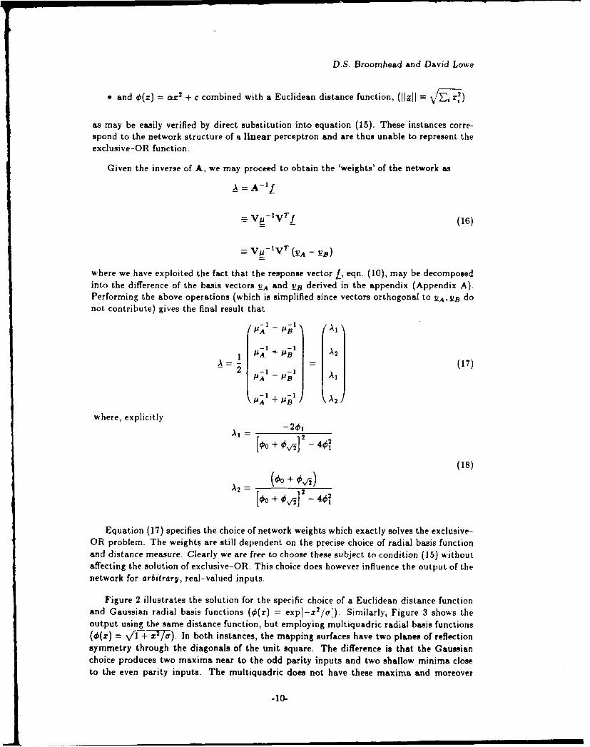
Equation (17) specifies the choice of network weights which exactly solves the exclusive-OR problem. The weights are still dependent on the precise choice of radial basis functionand distance measure. Clearly we are free to choose these subject to condition (15) withoutaffecting the solution of exclusive-OR. This choice does however influence the output of thenetwork for arbitrary, real-valued inputs.

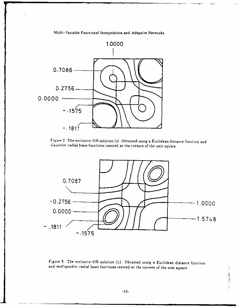
Figure 2 illustrates the solution for the specific choice of a Euclidean distance functionand Gaussian radial basis functions (0(z) = exp[-x 2/aj). Similarly, Figure 3 shows theoutput using the same distance function, but employing multiquadric radial basis functions(0(.T) =v/+-- ). In both instances, the mapping surfaces have two planes of reflectionsymmetry through the diagonals of the unit square. The difference is that the Gaussianchoice produces two maxima near to the odd parity inputs and two shallow minima closeto the even parity inputs. The multiquadric does not have these maxima and moreover

-10-

Multi- Variable Functional In terpolation and Adaptive Networks

1.0 000

0.0000

-. 1811

Figure 2: The exclusive-OR solution (i). Obtained using a Euclidean distance function andGaussian radial basis functions centred at the corners of the unit square.

0.7087

01.0000

1.574B

-. 1575

Figure 3: The exclusive-OR solution (Ii). Obtained using a Euclidean distance functionand niultiquadric radial basis functions centred at the corners of the unit square.


diverges rapidly outside the unit square. This distinction is of no relevance to the exclusive-OR function itself. It would however, be significant were it attempted to give meaningto input and output values other than those represented by zero and unity. Clearly, thedetails of the generalisation would then be dependent on the specific interpolation schemerepresented by the network.

We conclude this section with a discussion on the number of 'hidden units' employedto solve the problem. Note that the problem has been solved exactly; given the weightsas determined by eqn. (18) and a specific choice of a radial basis function, applying any ofthe input pattern pairs will guarantee to get the correct output answer. On preliminaryinspection this may not seem so surprising since each possible input data point was used asa centre for a radial basis function and so a 'dictionary' of possibilities could be encoded.'

One can exploit the symmetry of the solution however, to show how it is still possibleto solve the exclusive-OR problem exactly without explicitly specifying the response ofthe whole set of input states. Specifically, from eqn. (18) and by a judicious or 'fortuitous'choice of nonlinear function 0 (for instance if 01 = 0 or 0 = -OV2-) then two of the fourpossible weights would be zero. This uncouples the corresponding pair of hidden units fromthe system, with the result that the remaining network satisfies the exclusive-OR functionwithout being explicitly 'trained' on the entire possible set of input/output pairs.

1

2

Figure 4: Equivalent network for ex- Figure 5: Equivalent network for ex-clusive-OR with A2 set to zero. clusive-OR with A, set to zero.

For the case that 01 = 0 (Figure 5) the two identical weights connecting the two hiddenunits to the output unit have a value of 1/10 + r, I. In this case, the hidden units centredon the patterns (0, 0), (1, 1) have no connections to the output and hence cannot contribute.Thus, when these patterns are presented to the network, the two units which would reactmost strongly to their presence have been disconnected from the output unit while theremaining two respond with 01 = 0 as expected. Alternatively, if the patterns (0, 1), (1,0)are presented, one hidden unit contributes a value of 4'o and the other a value of 0/2. Sincetheir sum is just I/A 2 the result of the network is to give the answer I as it should. Asimilar argument may be presented for the case when 0 =-- -,2

In either case, the surfaces shown in Figure 2 and Figure 3 are constrained sufficientlyfor the specification of just two points to fix the remaining pair of output values. Here

3 However, note that this scheme has achieved a fit with four adjustable parameters, the weights Ai, whereasthe standard 2-2-1 multi-layer perceptron would employ nine adjustable parameters.

-12-


we have, by a suitable choice of 0, adjusted the form of the fitting algorithm to admit anetwork which 'generalises' the incomplete training data to give the entire exclusive-ORfunction. This sort of procedure can of course be employed by a multi-layer perceptron

However, it should be clear that for a strongly folded surface such as represents theexclusive-OR function (or the more general n-bit parity function shown in Appendix B) thepresence or absence of redundant points which may be omitted from the training set mustdepend sensitively on the implicit fitting procedure employed by the network. Moreover,the question of which points are redundant must also require detailed specific knowledge ofthe network and the relationship it is being used to represent. As a rule, one can expecta network to be capable of 'correctly' generalising, only when there is sufficient trainingdata appropriately distributed to enable an adequate fit to significant turning points of theunderlying graph. Clearly, the more folded this graph is, the more demanding will be therequirment on the data.

5 An analytic solution to a non-exact problem:The exclusive-OR problem with two centres.

The previous section, with its related appendices, dealt with exact solutions to strict inter-polation problems. For strict interpolation the interpolating surface is constrained to passthrough all the training data points. This is achieved by using the formalism described inthe first part of section 2. which requires the use of a radial basis function (or hidden unit)for each distinguishable data pair. It was noted that this rule may be relaxed in specialcircumstances where the symmetry and other details of the problem may be employed.

In this section we shall consider a specific example of the more general approach dis-cussed at the end of section 2 which relaxes the strict interpolation of the data. In addition,recall that in section 2, sufficient scope was allowed in the variant of radial basis functiontechniques to accomodate an approximate interpolating surface whereby this surface isnot directly constrained to go through all (or any) of the training set. This is clearly anadvantageous strategy when the input data is corrupted by external sources and it wouldnot be desirable to try and fit the noise added to the (presumably) structured data. Inaddition, where the true data actually represents a smooth map, it allows the use of farfewer hidden units than data points.

We repeat the analysis of the exclusive-OR problem considered in the previous section,but using just two radial basis function centres. It is clear that there are two distinct choiceshow the two centres may be positioned: either on opposing vertices, or adjacent verticeson the ordered corners of the unit square. We choose the lucations of the centres to be onopposing vertices at (0,0) and (1, 1). This choice allows us to exploit the symmetry of theexclusive-OR function to allow its solution with fewer 'training' points than data points.

The total training data is the mapping depicted in Table 1. The calculations are per-formed using the pseudo-inverse technique with, and without, the use of an adjustable biason the output unit.

5.1 The approximate exclusive--OR without an output bias.

-13-


0.0787

0.00 000.1969

0.03 940. 27 56

0.1181 __ _0.3937

0.1575

0.433 1

0. 472 4

Figure 6: Contours of the approximate exclusive-OR solution, w~ithout an output bias.

-14-


Following section 2, we use the following form of interpolating functions:

SWz = E AMU( z- Yijl) (19)

where _y, - [0, 0]T , Y3 = 1, jT. The set {A,} is given by

.f, = -,(llT - fylil) ; = 1,2,3,4 (20)

so thatA = A~L (21)

where f is the same response vector as in the exact case, eqn. (10), and A+ is the pseudo-inverse of the (non square) transformation matrix

A- I i (22)02 -001 .01

From Appendix A, given the singular value decomposition of A

A = USVT

the pseudo-inverse is obtained as

A + = V(S- 1 )UT

= V(Sl)2vTA (23)

The matrix V is composed of the normalised eigenvectors of the matrix

ATA- (= ab (24)

wherea = 0 + 2,12 + (25)b = + 2 22

and the diagonal matrix (S-1) 2 is made up of the reciprocal of the eigenvalues of thecorresponding eigenvectors.

It is straightforward to verify that

V=2 1 -1)(6

and

( (1/[a+ b - ) (27)

Substituting these matrices into the pseudo-inverse expression, eqn. (23) and then intoeqn. (21) gives,

_ )(28)

-15-


whereAl 201j[a + b]

201_____ (29)4.02 + 1,00 + 0-!

This is the set of weights with minimum norm which minimises the least mean squarederror to all the training data. In fact the error, C, may be evaluated analytically to give

(0o+02) (30)

+ V12 + 0 202/2 (30)

An interesting point about this error, is that it will be zero if the radial basis functionsare chosen to be such that Oc0 = -02. This is precisely the condition mentioned at the endof the previous section in the discussion of how the exact exclusive-OR problem could besolved with only two radial basis function centres. In both instances the error is zero andthe interpolating map manages to perfectly 'learn' the training data. However, for generalchoices of radial basis function the solution as derived, does not reproduce the desired outputof exclusive-OR satisfactorily. For instance, Figure 6 depicts this solution using Gaussianradial basis functions and a Euclidean norm. The figure plots contours of equal 'height'produced at the output of the radial basis function mapping. The vertices of the unitsquare in the figure represent the logical values 00, 01, 11, 10. As seen, although the outputdiscriminates succesfully between even and odd parity inputs, the relative magnitudes havenot been preserved (the output of 00 is greater than the output of 01 for instance). Thissituation is rectified by the inclusion of a 'bias' attached to the output node as is nowdemonstrated.

5.2 The approximate exclusive-OR including an output bias.

Consider the same situation as in the previous subsection, but where now a data independentvariable is allowed, effectively a weighted bias at the output node through a connection toa node which gives a constant unit output. The interpolating function now has the form

S(z) = Ao + E ,0(II - Il) (31),j=1,3

where {A1,3 } are as previously assumed. The problem is to fit three parameters by usingthe same four training points

The matrix of distances is now

A 1.. 0 I 1 01 (32)

1 02 00

1 01 01

Consequently, the singular value decomposition is determined by the eigenvectors andeigenvalues of the matrix

ATA= c a b (33)c b a

-16-


2.4409-

2. 2835 2.2835 /0.7087

1.9685 / 0.0000

1.5748 ,

-. 1811 - .1575

0.2756

Figure 7: Contours of the approximate exclusive-OR solution, including an output bias.

where

a + 2 2 +02

b 202 + 21,012 (34)

c = Oo + 201 + 0'2

Note that c here has the interpretation of being proportional to the mean value of radialbasis functions evaluated at any training point.

Consider the eigenvalue equation

ATA C12 0j2(03 03

From the characteristic equation one finds that the eigenvalue problem factorises, giving

IAO a - b

(a + b + 4) ± v/(a + b - 4)2 + 8c 2 (35)

2

The normalised eigenvector corresponding to p = a - b is then

ao = 1 (36)

.17-


For the case p = p±, we have a2 = a03 , since the resulting eigenvectors are orthogonalto a0 . Setting a 2 I without loss of generality implies that the (unnormalised) componental is

at = 2cP± - 4

Thus the resulting orthonormal matrices V and (S- 1 )2 take the form

/ 0 a+/A+ aj-/A..7- ,F 1// /A+ I/A_ (37)

-I/v V_ I/A+ l/A_

(s- A= 2.+ (38)0 0 A-

where the normalisation factors A± are given explicitly by

(A±) 2 2 + (a,) 2 (39)

Using these matrices to construct the pseudo-inverse of A results finally in the set ofweights,

A: x (40)A 0

where

A0= 204 (a+ + 246) + 2aj (a- + 21)A+A2 .u-A+

(41)kl- 2 2

A, = 2 (a+ + 201) +.--..r2 (a- + 201)P+&2+1A

This result is shown in Figure 7 and may be compared directly with that of the previoussubsection shown in Figure 6. Note that the network now succesfully discriminates statesof opposite parity and moreover returns precisely the correct magnitude for each corner ofthe unit square. However, the symmetry of placing the centres on the diagonal of the unitsquare, means that the solution obtained in this case is exact. There are only three inde-pendent equations we need to solve, and three adjustable parameters at our disposal. If wehad chosen our centres to be adjacent vertices of the unit square, then the symmetry wouldnot have existed to reduce the system of four equations to just three, and the approximateanalysis would not have produced a zero-error mapping.

We choose to interpret the action of the output bias in the following way. The r6le ofthe output bias rests on the fact that the desired output states of the exclusive-OR functionhave non-zero mean. The analysis without the inclusion of bias achieves a minimum errorsolution which matches the output in the mean. However, since positive weights are neededto achieve this, the resulting s(_) naturally has maxima near to the centres (0,0), (0, 1).Therefore, s(z) does not reproduce the required qualitative details of the exclusive-ORfunction. In contrast, the inclusion of the bias allows the whole surface s(;) to be 'floated'

to the correct mean level while the remaining parameters adjust its qualitative form.

-18-


It is interesting to repeat the calculation of section 5.1 using a response vector f(-2, 2, 2 ). This allows one to study an equivalent problem with the mean artificially

removed. This produces, again, two equal weight values (compare with (29))

=82 + 2[Oo + 0212

The resultant fit does not reproduce the training values as well as the three parametermodel given above. It does however have the correct qualitative form. The extra bias

parameter provides a compensation for a global shift which is hard to achieve throughweighting the individual basis functions. The consequences of this observation may also benoted in conventional multi-layer perceptron studies where the performance of the network

is enhanced if the input data is previously scaled to have zero mean.

6 Numerical examples:the prediction of chaotic time series.

Lapedes and Farber [13] have recently used multi-layer perceptrons for the prediction of timeseries data generated by nonlinear dynamical systems. Extensive comparisons with otherprediction techniques showed that multi-layer perceptrons were more accurate than the

classical (linear) methods and were comparable with the locally linear approach of Farmerand Sidorowich [161. In this section, we shall, following Lapedes and Farber, use nonlinear

prediction as a non-trivial example of the application of adaptive networks. We note thatin this application our approach is very close to that of Casdagli [17] who has applied

radial basis functions to the construction of nonlinear maps from time series data. Unlike

Casdagli who used strict interpolation, we shall employ the least squares generalisationgiven in section 2.

Specifically, consider T d, an ordered sequence of iterates of the doubling map:

x,+1 = 2x, (modulo 1) (42)

and T q, a sequence of iterates of the quadratic map

Xn+l = 4zn(1 - Xn) (43)

These maps are known to be chaotic on the interval [0, 11: in both cases the iterates ofgeneric initial conditions are distributed according to continuous invariant measures. For

Td the autocorrelation (xzoz) decays as 2 while for T-, (xOXn) - 60,n where 6,,, is theKroenecker delta. Therefore, given only the data Tq, second order statistics would conveythe impression that the sequence is random broadband noise (see Appendix C for furtherdetails). Naively (and in fact, erroneously) one might expect from this that the predictionof T q is harder than the prediction of Ti.

A radial basis function network for predicting one time step into the future was con-structed as follows. The basis function centres {y,} were chosen to be uniformly spaced

on (0, 1) - the number of centres was an adjustable parameter. A set of input values

{xi E [0, 11 t= 1,2,...,250) was used to calculate the matrix A using equation (4). The

singular value decomposition of A, calculated numerically by a Golub-Reinsch algorithm,

-19-


0

0 1Figure 8: The Quadratic Map: A figure showing the actual (solid line), and predicted (filledsquares) outputs of the network over the interval 10, 1) for one iterate.

was used to form the pseudo inverse A + using equation (46). This was then applied to thevector of outputs:

L (f(x,),.. f(x), f(X2 0))T

(where f(x) is the map given by either equation (42), or equation (43)) to obtain the weights

{ A,) according to A = A+f. The accuracy of this mapping were then analysed for an extra

250 different 'test' points.

Figures 8, and 9 which show the output of the networks as a function of inputs, illustrate

the relationship with curve fitting for these simple one-dimensional problems. It is clear

that the basis of the difference between predicting Td and predicting Tq is that the doubling

map is discontinuous and therefore hard to fit. Multi-layer perceptrons also have difficultywith trying to find an appropriate set of weight values which allows a good fit to Td (in fact

the overwhelming tendency is for the multi-layer perceptron to get stck in an unsuitablelocal minimum, M.D. Bedworth, private communication).

For prediction further into the future, the situation is further exacerbated and rapidlybecomes hard even in the case of Tq. The problem is now one of fitting a graph of then-th order iterate of equation (42) or (43). In either case the graph has 2n1 oscillationsof unit amplitude. In terms of the radial basis function network, this would require at least2n hidden units with centres appropriately positioned. An alternative to this strategy is to

iterate the one-step network. This however, is inaccurate since errors in chaotic systemsgrow exponentially because of the local instability of the evolution.

The accuracy of the network can be quantified by the following index, .:

r (Xzprdided(t) - Xee2 (t)]2) (44)

-20-


0 a

0

Figure 9: The Doubling Map: A figure showing the actual (solid line), and predicted (filledsquares) outputs of the network over the interval 10, 11 for one time step into the future forthe doubling map.

This quantity is a measure of how well the network generalises beyond the trainingdata. The error expression given in section 2 has the same form, but since it is based onthe training data, shows how well the network reproduces the training data. It is of interestto compare the two since the difference quantifies the degredation of the predictive powerof the network when it is required to generalise. The graphs shown in Figures 10 and 11summarise both kinds of error analysis for networks trained on Td, and T.

The most obvious difference between these figures is the scale. It is clear that predictionof Tq, whichever error criterion is used, is much easier than the prediction of Td by severalorders of magnitude. Beyond this, we see in both cases that the training error of section 2 hasthe same basic dependence on the number of hidden units; that is, a fast improvement as noincreases to about 30 followed by a plateau region where the relative improvement is small.As no approaches the number of data points used in the training (250 in this example),the training error again drops rapidly as the problem approaches the strict interpolatonlimit. This drop is not, however, mirrored by a drop in the recognition error. Althoughinitially, the recognition error follows the training error very closely, a saturation plateau isreached and approximately maintained irrespective of hov. many hidden units are employed.This can be understood sijice the capability of the model to generalise, is connected withthe underlying 'smoothness' of the true map and the level of 'smoothness' built into themodel through the choice of metric and radial basis function (and indeed the assumptionthat an arbitrary function may be approximately represented by the radial basis functionexpansion). Therefore one can surmise that in most instances, there will be a limitingaccuracy to which it is possible to model unseen data generated by a mapping. This isnot true for the training points themselves, since it is possible by strict interpolation toproduce a mapping surface which exactly passes through all the points. However, all thatthis accomplishes is a fit to the noise on the training points which may oscillate wildlybetween the constraining 'knots'. It was for this very reason that we introduced the leastsquares solution of the radial basis function construction in section 2.

-21-


Number of Centres

50 100 150 200I 1 I

-5

0 0. 0 0 0 0 0

-10 "

-15

logio(normalised error)

Figure 10: The Quadratic Map: The log normalised error showing the training (solid circles)and recognition data (open circles) as a function of the number of radial basis functioncentres. Euclidean norm and a Gaussian radial basis function (4 = exp[-z 2 no/161) were

used.

-22-


Number of Centres

50 100 150 200I I I I

-0.50 0

080

0 0 0

0 0

* 0

-1.0 * 0 0 0 0 00

0 0

0-.•0

0-1.5.

loglo(normalised error)

Figure 11: The Doubling Map: The log narmalised error showing the training (solid circles)and recognition data (open circles) as a function of the number of radial basis functioncentres. Euclidean norm and a Gaussian radial basis function (€ = exp[-z2ng/161) wereused.

-23-


7 Conclusion

The object of this paper has been to introduce a simple view of network models as devicesfor the interpolation of data in multidimensional spaces. The purpose of this is to allow theapplication of a large body of intuition and knowledge from the theory of fitting and interpo-lation to the understanding of the properties of nonlinear networks. Thus we associate theconcept of generalisation in networks with the simple idea of interpolation (extrapolation)between known data points. The details of the generalisation are then dependent upon theimplicit interpolation scheme employed by a given network. Generalisation is hard wherethe relationship has strong oscillations or discontinuities. This suggests that, particularlyin the case of abstract problems for which the topology of the input and output spaces maynot be clear a priori, it may be advantageous to attempt to code the data so as to producea relationship which is as smooth as possible. Further we expect the training data, wherepossible, would best be distributed to give information about all the turning points of thegraph and need not be tightly clustered where, for example, the relationship is smooth ormonotone.

Motivated by this philosophy, we introduce a network model based on the radial basisfunction approach to curve fitting. This model has two main advantages. First, it isfirmly attached to a well established technique for fitting, but, since it is contained withina general class of nonlinear networks, it may be used as a source of 'existence proofs' forsuch networks. For instance, we know that networks of this form can be used to modelrelationships which lie in the function space spanned by the chosen set of radial basisfunctions. The characterisation of this space and quantification of such things as the rateof convergence of radial basis function expansions is currently receiving much attention andis seen to be of direct relevance to the theory of networks.

The second advantage of this network is in practical application. The basis of its sim-plicity is that it combines a linear dependence on the variable weights with an ability tomodel explicitly nonlinear relationships such as for example, the exclusive-OR function.Thus, in the least squares context, training the network is equivalent to solving a linearmatrix equation. If we specialise to a minimum norm solution, the solution is unique andin this sense the network may be said to have a guaranteed learning algorithm.

This general approach, whereby optimisation is carried out on the subset of the weightsfor which the problem is linear, may be taken with other network models. It would beinteresting to study how much this restricts their generality. Work along these lines iscurrently in progress. In the present case, on the other hand, the inclusion of the basisfunction centres into the optimisation calculation may be carried out using a nonlinearoptimisation technique in conjunction with the hnear analysis described above. By analogywith spline fitting of curves, this may produce some advantage, perhaps in the form ofneeding fewer hidden units, but, it is questionable whether this would compensate for theadded complexity of performing the nonlinear optimisation. We have not approached herethe general question of what form of 4 is best, or where and how many centres should beused in the expansion. Work is currently in progress to assess the sensitivity of convergenceof these factors and the use of the error function given in equation (7) as a cost functionfor nonlinear optimisation using the basis function centres.

-24-


Acknowledgements

We would like to thank Professor M.J.D. Powell at the Department of Applied Mathematicsand Theoretical Physics at Cambridge University for providing the initial stimulus for thiswork. Also, we appreciate the help given to us by Mark Bedworth, John Bridle and AndrewWebb of the Speech Research Unit at RSRE for sharing their insights into the workingsof layered network models in general, and the difficulties associated with the practicalapplication of the logistic, semi-linear multi-layer perceptron in particular.

-25-


A Solving linear inverse problems.

The appendix looks at linear inverse problems as they arise in the radial basis functionapproach to nonlinear networks.

In applying the radial basis function method, we need to invert an m x r (M > n)matrix with elements A,, = 0(lix - V,11). Since A may be rank deficient, it is necessary to

account for the possibility of ill-conditioning. Consider the singular value decomposition ofA

A = USVT (45)

where V is an n x n orthogonal matrix, S is an n x n diagonal matrix of singular valuesand U is an in x n marix with orthonomal columns. The pseudo inverse of A, A4 , maybe constructed as

A- = VS+U r (46)

where S + is obtained from S by reciprocating the non-zero diagonal elements. Clearlyif rankA=- m then A 4 A = 1 where 1 is the m x m unit matrix. On the other hand,AA' = UUT a superposition of projections onto a subspace of F' spanned by the columnsof U. If rankA< m then A'A and AA' give projections onto subspaces of IRm and Rn

respectively.

In the case of the exact exclusive-OR function the question of ill-conditioning doesnot arise. In this case it is convenient to calculate the inverse of A through its eigenvaluedecomposition since the symmetry of the problem may be exploited to obtain the solution.Here

A = VpVT (47)

where, since in this case A is a real symmetric matrix, the matrix of eigenvectors V isorthogonal. It follows that

A - ' = Vu-IVT (48)

assuming that A is full rank. The rest of the appendix deals with the calculation of theeigenvectors and eigenvalues of A using the symmetry of the exclusive-OR function.

Our choice of ordering of the input points in section 4 is somewhat arbitrary. It shouldbe clear that we can perform a sequence of rotations on the original orderings while retainingthe same matrix A. In other words, A is invariant to a certain class of transformations, inparticular, it is invariant to operations in the group C 4 = {E, C4 ,C 2 ,C }, where E is theidentity transformation, C 4 denotes rotations by 7/2, C2 by 7r and C4 rotations by 37r/2.

The character table for the group C4 is shown in Table 2 (for an introduction to the theoryand application of groups see [191).

The character table may be exploited to solve the eigenvalue problem for A by obtaininga symmetry adapted basis. We can see this as follows. The representation of the groupoperations using the standard basis,

-€1 = (I f2= ( -- = ( C4 = (-

-26-


C4 E C4 C2 C4

A 1 1 1 1B 1 -1 I -I

E -

Table 2: The character table for C4

is not irreducible since it's dimension is four and the maximum dimension of an irreduciblerepresentation of C4 is two. In fact this representation of the group has the form r =A + B + E and so the basis has irreducible components A, B, E. From the character table

one can ascertain that the appropriate symmetry adapted basis is just

L-A = vB !!IEE=_ = -

or, by normalising and replacing the degenerate vectors YE and vi by simple linear combi-nations, we arrive at a symmetry adapted set of basis vectors,

1 1 1 1

k-A= 2 LB -r=2 E 2= _0 v/2 E 2 0(49)

It is clear that these basis vectors are orthogonal and they are eigenvectors of the matrixA since, explicitly,

AYVA = (o+20,+ V)VA A o( 0+201+40-)

AYB = (0 - 20, + 0' )-' AB = (0o - 20, + ,.,) (50)A dv = ('00 - 0 ,r)_vl AE = (00 - OV 2)

These basis vectors and eigenvaluee are employed in section 4 to obtain a set of weightsanalytically, which exactly solves the exclusive-OR function.

-27-


B An analytic solution of the exact n-bit parity problem

The n-bit parity problem is a generalisation of the exclusive-OR problem discussed insection 4. It may be defined by the mapping depicted in Table 3, that is, the output isunity if fhe tota! number nf input bits having value one is odd, otherwise the output is zero.Thus changing one bit in the input pattern produces a maximal change in the output.

Input Number of 'ON' OutputPattern bits in input Pattern

000 -, 0 -. 0001 - 1 -, 1010 - 1 1100 -. 1 - 1011 2 -. 0101 - 2 - 0110 -. 2 - 0111 -- 3 - 1

Table 3: Symbolic mapping of the n-bit parity problem for the case n = 3.

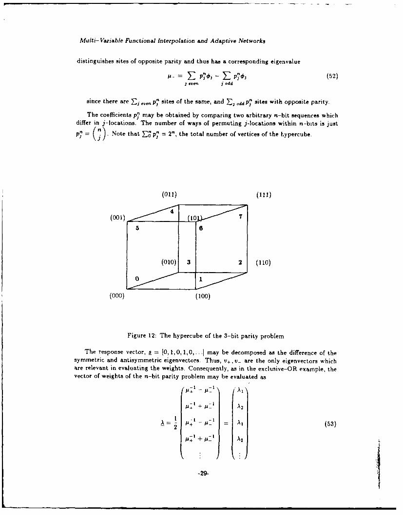
With the benefit of insight deve!oped from the exclusive-OR problem, this section ob-tains an exact representation of the n-bit parity problem as a network based on radialbasis functions. The network will have the general form of n-inputs for an n-bit word,and 2" hidden units all connected to one output. The centres of the 2" hidden units cor-respond to the possible input patterns. Thus, an exact solution may be obtained once the2"-dimensional vector A of weights has been determined. All possible input states may beput in a I : I correspondence with the vertices of a unit n-dimensional hypercube. Thisis conveniently achieved by aligning the hypercube with the Cartesian basis so that onevertex resides at the origin. The Cartesian co-ordinates of each vertex then directly mapsto a unique binary sequence, for instance (0,0,0) - 000, (0, 1,0) - 010, (1, 1,0) - 110,etc. The vertices may be ordered by treating the set of sequences as a cyclic Grey codeof the first 2" integers. Thus all nearest neighbours in this scheme correspond to points ofopposite parity and the use of the cyclic Grey code ensures that entries across the rows ofA represent points of alternating parity.

The rows of A are permutation of each other because of the symmetry of the hypercube.It follows that there is a totally symmetric eigenvector, v+ = 2n/211", 1,. IT for which thecorresponding eigenvalue is the sum of the row elements of A

'1

1=0

where p. is the number of j-th nearest neighbours to an arbitrary vertex.

A second eigenvector may be found using the division of the vertices into two groups,differentiated by their parity. The form of this eigenvector follows from the use of the cyclicGrey code in ordering the vertices: v- = 2-n/2[l, -1, ,...]7. This antisymmetric form

-28-


distinguishes sites of opposite parity and thus has a corresponding eigenvalue

IA-_ ZPno,-ZP7 , (52)2 even j odd

since there are Fj even p,1 sites of the same, and Ej odd P' sites with opposite parity.

The coefficients p7 may be obtained by comparing two arbitrary n-bit sequences whichdiffer in j-locations. The number of ways of permuting j-locations within n-bits is just

()Note that Enp7 = 2 nthe total number of vertices of the hypercube.

(011) (111)

4(001) (107

5 6

(010) 3 2 (110)

(000) (100)

Figure 12: The hypercube of the 3-bit parity problem

The response vector, s = [0, 1,0, 1,0,.. . may be decomposed as the difference of thesymmetric and antisymmetric eigenvectors. Thus, v+, v- are the only eigenvectors whichare relevant in evaluating the weights. Consequently, as in the exclusive-OR example, thevector of weights of the n-bit parity problem may be evaluated as

u. t + )-_'+ Mu- A2

2--- A A1 (53)

P+ + A- 2

-29-

I


where,

= - odd (7) 0j[rjeven ( 0~jJ2. [Fj odd ) 12

(54)

A2 =even

Equation (54) accomplishes what the section set out to obtain: an exact solution to then-bit parity problem in the sense that there is a guaranteed set of values for the weights ofthe matrix which ensures that the result of the network is to reproduce, at least, the valuesexhibited in Table 3. It should be noted that although this task has been achieved witha network involving 2' hidden units, it is still possible to solve the problem exactly withfewer than this number of hidden units. For instance, and by analogy with the exclusive-OR problem, if the radial basis function and metric were chosen in such a way that either

of z3 even (55)

j odd

are satisfied, then an exact solution may be obtained with only 2n - 1 hidden units.

-30-


C The quadratic and doubling maps

This appendix lists a few details relevant to the chaotic maps discussed in section 6 for timeseries prediction. The quadratic map, as discussed, determines the signal at time t + 1 interms of the signal at time t by the explicit iteration scheme

t+, = 4z,(I - x,) (56)

By a simple linear transformation, x - y, this map is transformed into the form

y,-+, 2 - 1 (57)

Since these two mappings are related by a linear transformation (z = 0.5[1 - y]), thebehaviour of equation (57) determines the behaviour of the quadratic map. Equation (57)is interesting because it illustrates that the mapping is explicitly given in terms of Chebyshevpolynomials 1201, specifically

Y.+1 = T 2(!j.) (58)

From this relationship and exploiting the property of Chebyshev polynomials that

2TroT. = T.+,,, + T._,, (59)

or, specifically2T' = T 2, + To (60)

one finds that the n-th iterate, yr, is connected with the starting value yo through the 2"Chebyshev polynomial,

Yn = T2-(Y0 ) (61)

This just makes explicit the fact that the value of the map at any time in the futureis uniquely determined by the starting value. However, the map is known to be ergodic,and thus time averages are equivalent to phase averages. To obtain the phase average, oneneeds the fact that the invariant measure of the map, eqn. (57), is

1m(Y) = (62)7rv, y 2

Therefore, the correlation function (ykYk+,) may be determined by the expectation value

S T2k (Yo)T 2&+, (Yo'= o dyO (63)

However, this is precisely the orthogonality relationship between Chebyshev polynomialsof the first kind, and hence the integral yields a Kroeneker delta,

(9k+, = b6,.O (64)

Consequently, as far as second order statistics are concerned, the time series generatedby the quadratic map totally loses its memory between each time step, and hence would

-31-


appear to be an infinite bandwidth, noise signal (this is of course not the case when higherorder correlations are taken into account).

In the case of the doubling map, the value of the time series at time t + I is determinedby the time series at t via

xt+l = 2zt mod 1 (65)

The correlation function may be expressed as

( xz) = xo12'xol dx

(66)=2'- 1/,+ 1)/2f x[2'x] dx2-1(J+ )/2

j=O f/

where [x] denotes the fractional part of x (note that the invariant measure is uniform inthis case and the map is known to be chaotic so that time averages and ensemble averagesare equivalent). By a change of variables, y = 2'x-j the above integral is readily performedto give:-

(xzoj) 2 2 +~3 2, =0

(67)

4 3

Thus, in contrast to the quadratic map, the correlation function for the doubling mapdecays exponentially in time.

-32-


References

[11 F. Jelinek, R.L. Mercer and L.R. Bahl, "Continuous Speech Recognition: Statistical

Methods", "Handbook of Statistics", 2, edited by P.R. Krishnaiah and L.N. Kanal,

(North-Holland Publishing Company, 1982), 549-573.

[2] S.E. Levinson, L.R. Rabiner and M.M. Sondhi, "An Introduction to the Applicationof the Theory of Probabilistic Functions of a Markov process to Automatic Speech

Recognition", The Bell System Technical Journal, 62(4), (1983), 1036-1073.

[31 L.R. Rabiner, J.G. Wilson and B.H. Juang, "A model-based connected-digit recog-

nition system using either hidden Markov models or templates", Computer Speech &

Language, 1(2), (1986) 167-197.

[4] D.E. Rumelhart, G.E. Hinton and R.J. Williams, "Learning Internal Representations

by Error Propagation", ICS Report 8506, (1985), (Institute for Cognitive Science,

University of California, San Diego).

[5] Mark D. Bedworth and John S. Bridle, "Experiments with the Back-Propagation

Algorithm: A Systematic Look at a Small Problem", RSRE Memorandum 4049,(1987), (available from R.S.R.E., St. Andrews Rd., Great Malvern, Worcs. WR14

3PS, England.)

[6] D.C. Plaut, S.J. Nolan and G.E. Hinton, "Experiments on Learning by Back Propa-

gation", CMU-CS-86-126, (1986), (Carnegie-Mellon University).

[7] M.J.D. Powell, "Radial basis functions for multivariable interpolation: A review",

IMA conference on "Algorithms for the Approximation of Functions and Data",

RMCS Shrivenham, (1985).

[81 Charles A. Micchelli, "Interpolation of Scattered Data: Distance Matrices and Condi-

tionally Positive Definite Functions", Constructive Approximation, 2, (1986), 11-22.

[9] R. Franke, "Scattered Data Interpolation: Tests of some methods", Mathematics and

Computing, 38, (1982), 181-200.

[10] G. Golub and W. Kahan, "Calculating the Singular Values and Pseudo-Inverse of a

Matrix", Journal SIAM Numerical Analysis, Series B, 2(2), (1965), 205-224.

[11] J.C. Nash, "Compact Numerical Methods for Computers: linear algebra and function

minimisation", (Adam-Hilger Ltd, Bristol, 1980)

[121 William H. Press, Brian P. Flannery, Saul A. Teukolsky and William T. Vetterling,"Numerical Recipes: The Art of Scientific Computing", (Cambridge University Press,

1986)

[131 Alan Lapedes and Robert Farber, "Nonlinear Signal Processing using Neural Net-works: Prediction and System Modelling", (submitted to Proceedings of IEEE, July

1987).

[14] Raymond L. Watrous, "Learning Algorithms for Connectionist Networks:AppliedGradient Methods of nonlinear Optimisation", (1987).

-33-


[15] M.J.D. Powell, "Radial basis function approximations to polynomials", DAMPTpreprint 1987 NA/6, (presented at the 1987 Dundee biennial Numerical AnalysisConference).

[16] J. Doyne Farmer and John J. Sidorowich "Predicting Chaotic Time Series", PhysicalReview Letters, 59,(8), (1987), 845-848.

[171 Martin Casdagli, "Nonlinear prediction of chaotic time series", (Submitted to PhysicaD 1988)

[18) ]an D. Longstaff and John F. Cross "A pattern recognition approach to understandingthe multi-layer perceptron", Pattern Recognition Letters,5,(1987), 315-319

[19] L.D. Landau and E.M. Lifshitz, "Quantum Mechanics: Non-Relativistic Theory",(Pergammon Press, 2nd edition 1965, Chapter XII)

[20] Milton Abramowitz and Irene A. Stegun, "Handbook of Mathematical Functions",(Dover Publications, Ninth Edition, 1970)

-34-

Co0py available to DTIC do" DODOCUMENT CONTROL SHEET permit tu'll legible ,elptodcti n

UNCLASSIFIEDOverall security classification of sheet . . . LA.S. . . ..D

(A far as possible this sheet should contain only unclassified information. If it is necessary to ener

classified information, the box concerned must be marked to indicate the classification eg (R) (C) or ( )

1. DRIC Reference (if known) 2. Originator's Reference 3. Agency Reference 4. Report SecurityMEMO 4148 1U/C Clas- I c a -Cn

5. Originator's Code (if 6. Originator (Corporate Author) Name and Location

778400 known) ROYAL SIGNALS & RADAR ESTABLISHMENT, ST ANDRE-v'S RzZGREAT MALVERN, WORCESTERSHIRE WR14 3PS

5a. Sconscring Agency's 6a. Sponsoring Agency (Contract Authority) Name and LocatiorCode (if known)

7. Title RADIAL BASIS FUNCTIONS, MULTI-VARIABLE FUNCTIONAL INTERPOLATI i

AND ADAPTIVE NETWORKS.

7a. Title in Foreign Language (in the case of translations)

7t. Presented at (for con 4erence racers) Title, place and date of conference

8. Author 1 Surname, initials 9(a) Author 2 9(b) Authors 3,4... 10. Date P.-. ref.BROOMHEAD, D.S. LOWE, D. 1988.3 34

11. Contract Number 12. Period 13. Project 14. Other Rsference

15. Distribution statement

UNLIMITED

Descriptors (or keywords)

continue on separate viece of oaver

Abstract The relationship between 'learning' in adaptive layered networks and the

fitting of data with high dimensional surfaces is discussed. This leadsnaturally to a picture of 'generalisation' in terms of interpolation between

known data points and suggests a rational approach to the theory of such networksA class of adaptive networks is identified which makes the interpolation scheme

explicit. This class has the property that learning is equivalent to the solu-tion of a set of Zinear equations. These networks thus represent nonlinear

relationships while having a guaranteed learning rule. 4-- ',

s8;i48. DTIC does not__~ ~ JJ to...' ' =DTI-Cmmmmm m m

unlimited - apps.dtic.mil

Documents