universitÁ degli studi di padoav corso di...

UNIVERSITÁ DEGLI STUDI DI PADOVA

Corso di Laurea Magistrale in

INGEGNERIA DELL'AUTOMAZIONE

Implementation of distributed partitioningalgorithms using mobile wheelphones

Relatore: Prof. Luca Schenato Laureando: Schiesari Pietro

Anno Accademico 2016-2017

Abstract

Multi-robot coverage of an area is a fundamental problem in robotics. This

thesis presents the implementation process of partitioning algorithms from the

theorical ideas to sperimental results. In particular, the algorithms used are

two versions of the classic Lloyd method based on centering and partioning for

the computation of Centroidal Voronoid partitions. The di�erences between

these versions are the communication architectures: client-server and peer-to-

peer. In the �rst architecture the robots are allowed to comunicate with a

central server-base station, whereas in the second one the robots communicate

among neighboring peers. Therefore the tests have been conducted �rst on a

simulated control system designed using the softwares Matlab and Simulink

and then on the control of mobile Wheelphones that are innovative robotic

platforms for smartphones.

1

Contents

1 Introduction 71.1 Motivation . . . . . . . . . . . . . . . . . . . . . . . . . . . . . . . . . 71.2 State-of-the-art . . . . . . . . . . . . . . . . . . . . . . . . . . . . . . 81.3 Original contribution . . . . . . . . . . . . . . . . . . . . . . . . . . . 91.4 Thesis overview . . . . . . . . . . . . . . . . . . . . . . . . . . . . . . 10

2 Experimental Apparatus 112.1 Wheelphone Hardware . . . . . . . . . . . . . . . . . . . . . . . . . . 112.2 Wheelphone Software . . . . . . . . . . . . . . . . . . . . . . . . . . . 122.3 Motion Capture . . . . . . . . . . . . . . . . . . . . . . . . . . . . . . 17

3 The Coverage: Formulation and Algorithms 213.1 Voronoi Partitions, Centroids and Multicenter Function . . . . . . . . 213.2 Problem Formulation and Selected Approachs . . . . . . . . . . . . . 223.3 Server-based Algorithm . . . . . . . . . . . . . . . . . . . . . . . . . . 233.4 Distributed Gossip Algorithm . . . . . . . . . . . . . . . . . . . . . . 26

4 Wheelphone Robot: modeling and control 294.1 Unicycle Model . . . . . . . . . . . . . . . . . . . . . . . . . . . . . . 29

4.1.1 Dynamic Modeling . . . . . . . . . . . . . . . . . . . . . . . . 294.1.2 Kinematic Modeling . . . . . . . . . . . . . . . . . . . . . . . 30

4.2 Motion Control . . . . . . . . . . . . . . . . . . . . . . . . . . . . . . 314.2.1 Inner-Loop . . . . . . . . . . . . . . . . . . . . . . . . . . . . 314.2.2 Outer-Loop . . . . . . . . . . . . . . . . . . . . . . . . . . . . 33

5 Numerical and Experimental Results 375.1 Preliminary Results . . . . . . . . . . . . . . . . . . . . . . . . . . . . 375.2 Pose Reconstruction with 3D Motion Capture System . . . . . . . . . 40

5.2.1 Marker Labelling . . . . . . . . . . . . . . . . . . . . . . . . . 405.2.2 Pose Reconstruction . . . . . . . . . . . . . . . . . . . . . . . 435.2.3 Implementation . . . . . . . . . . . . . . . . . . . . . . . . . . 44

5.3 Coverage Algorithms Simulations . . . . . . . . . . . . . . . . . . . . 465.3.1 Server-Based Algorithm Implementation . . . . . . . . . . . . 475.3.2 Gossip Distributed Algorithm Implementation . . . . . . . . . 48

5.4 Results . . . . . . . . . . . . . . . . . . . . . . . . . . . . . . . . . . . 51

6 Conclusions 59

7 APPENDIX 61

A Wheelphone Drivers 61A.1 sfun_wheelphone.c . . . . . . . . . . . . . . . . . . . . . . . . . . . 61A.2 sfun_wheelphone.tlc . . . . . . . . . . . . . . . . . . . . . . . . . . 66A.3 driver_wheelphone.c . . . . . . . . . . . . . . . . . . . . . . . . . . . 68A.4 wheelphonelib.tlc . . . . . . . . . . . . . . . . . . . . . . . . . . . . . 73

3

List of Figures

1 Wheelphone Robots . . . . . . . . . . . . . . . . . . . . . . . . . . . . 72 Wheelphone Components . . . . . . . . . . . . . . . . . . . . . . . . . 113 Phone-Robot Communication . . . . . . . . . . . . . . . . . . . . . . 124 Simulink Block Process . . . . . . . . . . . . . . . . . . . . . . . . . . 145 sfun_wheelphone . . . . . . . . . . . . . . . . . . . . . . . . . . . . . 156 Android Application's Life Cycle . . . . . . . . . . . . . . . . . . . . 167 Optical Motion Capture System . . . . . . . . . . . . . . . . . . . . . 178 Passive Markers . . . . . . . . . . . . . . . . . . . . . . . . . . . . . . 189 MAGIC Lab Con�guration . . . . . . . . . . . . . . . . . . . . . . . . 1810 Packet Structure . . . . . . . . . . . . . . . . . . . . . . . . . . . . . 1911 Voronoi Partition. . . . . . . . . . . . . . . . . . . . . . . . . . . . . . 2112 Client-Server Communication Architecture. . . . . . . . . . . . . . . . 2313 Peer-to-Peer Comunication. . . . . . . . . . . . . . . . . . . . . . . . 2614 Partitioning Process of GD algorithm . . . . . . . . . . . . . . . . . . 2615 A Gossip Distributed Iteration . . . . . . . . . . . . . . . . . . . . . . 2816 Motion Control. . . . . . . . . . . . . . . . . . . . . . . . . . . . . . . 2917 Odometry. . . . . . . . . . . . . . . . . . . . . . . . . . . . . . . . . . 3118 Tracking. . . . . . . . . . . . . . . . . . . . . . . . . . . . . . . . . . . 3119 Inner-Loop Controller. . . . . . . . . . . . . . . . . . . . . . . . . . . 3220 Linear Velocity Trend . . . . . . . . . . . . . . . . . . . . . . . . . . . 3321 Angular Velocity trend . . . . . . . . . . . . . . . . . . . . . . . . . . 3322 A Vehicle Trajectory . . . . . . . . . . . . . . . . . . . . . . . . . . . 3423 Outer-Loop. . . . . . . . . . . . . . . . . . . . . . . . . . . . . . . . . 3524 Application Simulink Scheme . . . . . . . . . . . . . . . . . . . . . . 3725 Phone-Computer Communication . . . . . . . . . . . . . . . . . . . . 3826 "Sequence of Points" Test1 . . . . . . . . . . . . . . . . . . . . . . . . 3927 Wheelphone Robot with Markers . . . . . . . . . . . . . . . . . . . . 4028 Robots Patterns . . . . . . . . . . . . . . . . . . . . . . . . . . . . . . 4129 Reference Model . . . . . . . . . . . . . . . . . . . . . . . . . . . . . 4230 Simulink Motion Capture Block Scheme . . . . . . . . . . . . . . . . 4431 "Sequence of Points" Test2 . . . . . . . . . . . . . . . . . . . . . . . . 4532 Gaussian Sensory Function . . . . . . . . . . . . . . . . . . . . . . . . 4633 Gaussian Sensory Function . . . . . . . . . . . . . . . . . . . . . . . . 4734 VoronoiBounded Output . . . . . . . . . . . . . . . . . . . . . . . . . 4735 Poly2Centroid Output . . . . . . . . . . . . . . . . . . . . . . . . . . 4836 Evolution of the Partition in GB algorithm . . . . . . . . . . . . . . . 5037 Initial conditions. . . . . . . . . . . . . . . . . . . . . . . . . . . . . . 5138 Evolution of Simulate Server Based Algorithm . . . . . . . . . . . . . 5239 Evolution of Experimental Server Based Algorithm . . . . . . . . . . 5340 Evolution of Simulate Gossip Distributed Algorithm . . . . . . . . . . 5441 Evolution of Experimental Gossip Distributed Algorithm . . . . . . . 5542 Evolution of the cost function H. . . . . . . . . . . . . . . . . . . . . 56

5

1 Introduction

Wheelphone is an innovative mobile platform for smartphones built in 2013 by GC-Tronics company. It allows mobile phones to move in the surrounding area thanks tothe presence of two wheels. Moreover the phone itself is the hardware that generatesthe movement of the platform.In this thesis we want to improve the capabilities of this device implementing on ittwo area partitionig algorithms. Their task is to divide the enviroment in regions inorder to position the robots in the most e�ective way to cover the area.

Figure 1: Wheelphone Robots

1.1 Motivation

Nowdays autonomous robots perform a broad range of tasks. Robotic camera net-works can monitor airports and other public infrastructures. Teams of vehicles canperform surveillance, exploration, search and rescue operations. Groups of robotscan have logistic capacities in the transportation of goods and in the delivery ofservices. There are many reasons for their use:

• Quality: for certain tasks that require high positioning precision and highrepeatability, robots can be better than humans in terms of work quality.

• Costs: the high level of produttivity, from one hand, and the reduction in thenumber of wages, from the other hand, make robot more pro�table.

• Safety: the application of robots is safer in certain situations such as workingwith dangerous materials or in extreme enviroment.

7

• Flexibility: a single robot can be used to perform multiple activities reducingtime and improving quality.

It is interesting to analyze the robot performance in the coverage area applicationbecause of its importantance in everyday life and its di�culty in implementing it.The coverage area topic consists in �nding the optimal robot position in order tooversee a speci�c area. More robots are used, the more di�cult it becomes to getgood results. In fact the choosen zone has to be divided into N partitions eachof which is associated whith a particular robot. Each robot has to monitor onlythe assigned sub-area. Moreover, assuming that the initial partitions and robotsposition into the area are not e�cient, the comunication between the vehicles isneeded. For this reason it is important to take into account the physical limitationsof the robots: the range of communication signal and the computing power.For example, considering a high communication range and a low computing power, itis better to use a server-based communication architecture; otherwise, with invertedvalues, it would be better to use a distributed architecture. In the �rst case therobots interact with an external server that has the task of performing calculationsand redirecting them. In the second one the robots, communicating indipendentlybetween them, decide their best location.Another interesting challenge in analysing this topic is that any single area pointcan not have the same importance. To better explain this concept we consider themonitoring of a forest by a group of robots for detecting possible wild�res. It is easyto see that there is a direct correlation between the level of temperature and thepossibility of �res, so the most important area points are the warmest. Assumingthat, the robots should sorround the areas with the higher level of temperatureleaving uncovered the other zones.All these considerations are on the basis of the development of this thesis whosegoal has been the implementation and the experimental validation of distributedpartitioning algorithms using Wheelphone robots.

1.2 State-of-the-art

The last few years have seen a fast progression in the eld of the robotic control andnew developments continue to expand the literature which presents continuouslynew solutions and approaches along with the arising of always new and harder chal-lenges.In the classical coverage literature, there are many works [1]-[4]-[5]-[6]-[10] thatpresent a gradient descent strategy for a class of functions which encode optimalcoverage policies. The authors exploit the concept of centroidal Voronoi partitionsto optimally divide the monitored area focusing on di�erent aspects. In [1] and [10]they consider a non-convex enviroment with the presence of obstacles whereas in[4]-[5]-[6] the coordination problems for networked robots are presented. In [12] theauthors propose a policy for the optimal coverage of a line with perfectly knownnon-uniform sensory function. In [7] only a limited number of noise-free samples ofthe sensory function are considered. Finally, a distributed solution to the coverageproblem in the presence of known time-varying density functions is presented in [11].Another research direction can be seen in [21]-[23]-[22] considering the sensory func-

8

tion not known by the robots. In these cases each robot independently estimatesthe function of interest based on its own measurements and those gathered by itsneighbors.We have also to consider what tasks Wheelphone robot can alredy perform. Thefollowing list shows the name and the feratures of the main Applications that canbe downloaded from the web.

• Wheelphone : visualize all the sensor information on the phone and imple-ment "move-around-on-table" behavior

• Wheelphone_follow : it allows the robot to follow an object in front of it,using the front facing proximity sensors

• WheelphoneRecorder : record video while moving

• WheelphoneFaceme : face-tracking application. It keeps track of the posi-tion of one face using the front facing camera, then controls the robot to tryto face always the tracked face

• WheelphoneBlobDetection : the Wheelphone robot follows a blob chosenby the user through the interface

• WheelphoneLineFollowing : it allows the robot to follow a black (or white)line on the �oor using the ground sensors.

• WheelphoneNavigator : environment navigation application. It allows therobot to navigate an environment looking for targets while avoiding obstacles.It has two modules to avoid the obstacles: (1) the robot's front proximitysensors and (2) the camera + Optical Flow.

1.3 Original contribution

The goal of this thesis is to describe the implementation process and comparison oftwo partitioning algorithms given Wheelphone robots.The starting point was to analyze the tecnical features of a single Wheelphone robotbecause, as is possible to see in the previous section, was not created for this typeof task. We veri�ed that we had the possibility to access the wheels speed and toset these data as we please. Once we have �nished the analysis, we were able toimplement a motion control algorithm to drive Wheelphone in a speci�c position.These were the basis for the realization of our algorithms.The next step was to select two algorithms with di�erent characteristics : once basedon a synchronous client-server communication architecture and the other based onan asynchronous and pairwise communication.Once chosen them, we identi�ed a cost function, named Multicenter Function, thatgave us the goodness of an algorithm in terms of proximity to the optimal robotsposition.Going more in deep, the real original contribution of this thesis was that all the abovedescription was implemented for a smartphone application. Nowdays everybodyhave smartphones which are an increasingly important part of day-to-day life. Many

9

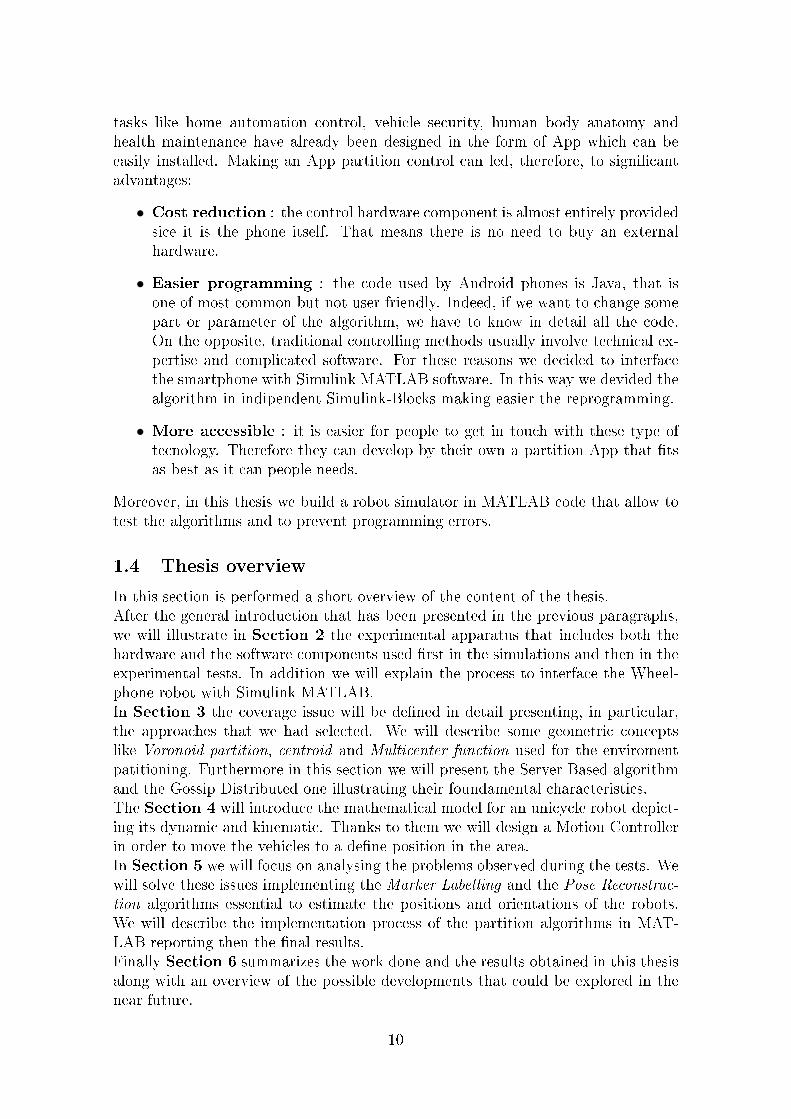
tasks like home automation control, vehicle security, human body anatomy andhealth maintenance have already been designed in the form of App which can beeasily installed. Making an App partition control can led, therefore, to signi�cantadvantages:

• Cost reduction : the control hardware component is almost entirely providedsice it is the phone itself. That means there is no need to buy an externalhardware.

• Easier programming : the code used by Android phones is Java, that isone of most common but not user-friendly. Indeed, if we want to change somepart or parameter of the algorithm, we have to know in detail all the code.On the opposite, traditional controlling methods usually involve technical ex-pertise and complicated software. For these reasons we decided to interfacethe smartphone with Simulink MATLAB software. In this way we devided thealgorithm in indipendent Simulink-Blocks making easier the reprogramming.

• More accessible : it is easier for people to get in touch with these type oftecnology. Therefore they can develop by their own a partition App that �tsas best as it can people needs.

Moreover, in this thesis we build a robot simulator in MATLAB code that allow totest the algorithms and to prevent programming errors.

1.4 Thesis overview

In this section is performed a short overview of the content of the thesis.After the general introduction that has been presented in the previous paragraphs,we will illustrate in Section 2 the experimental apparatus that includes both thehardware and the software components used �rst in the simulations and then in theexperimental tests. In addition we will explain the process to interface the Wheel-phone robot with Simulink MATLAB.In Section 3 the coverage issue will be de�ned in detail presenting, in particular,the approaches that we had selected. We will describe some geometric conceptslike Voronoid partition, centroid and Multicenter function used for the enviromentpatitioning. Furthermore in this section we will present the Server-Based algorithmand the Gossip Distributed one illustrating their foundamental characteristics.The Section 4 will introduce the mathematical model for an unicycle robot depict-ing its dynamic and kinematic. Thanks to them we will design a Motion Controllerin order to move the vehicles to a de�ne position in the area.In Section 5 we will focus on analysing the problems observed during the tests. Wewill solve these issues implementing the Marker Labelling and the Pose Reconstrac-tion algorithms essential to estimate the positions and orientations of the robots.We will describe the implementation process of the partition algorithms in MAT-LAB reporting then the �nal results.Finally Section 6 summarizes the work done and the results obtained in this thesisalong with an overview of the possible developments that could be explored in thenear future.

10

2 Experimental Apparatus

This section presents the experimental apparatus used �rst in the simulations andthen in the experimental tests.All the simulations are run in MATLAB R2015b on a laptop with a processor IntelCore i3 and 4Gb of RAM. The tests, instead, are focus on the control of a roboticplatform for smarphones, Wheelphone, whose hardware and software componentswill be respectively illustrated in Sections 2.1 and 2.2. We instantiated the partition-ing algorithms in the smartphone Samsung GALAXY S3 mini through the MATLABSupport Package for Android Sensors. Finally, to perform a better motion control,we used the Motion Capture System of Padova's Engineering Department whosefeatures will be described in Section 2.3.

2.1 Wheelphone Hardware

Wheelphone is a vehicle with two parallel wheels, each one mounted beside theircenter. It is able to steer thanks to a sliding surface placed on the front side of therobot. The Figure 2 shows the components of a Wheelphone and the Table belowdescribes its features.

Figure 2: Wheelphone Components

Feature Tecnical Information

width 92 mmlength 102 mmheight 66 mmweight 200 gdistance between wheels 92 mmwheel diameter 68 mmbattery LiPo rechargeable battery (1660 mAh, 3.7 V)processor microchip PIC24FJ64GB004; 16 MHzmemory RAM: 8 KB; Flash: 64 KB

ssssss

11

Wheelphone vehicle has two direct current (DC) geared motors, one for wheel, thatcan drive the robot with a maximum speed of 30 cm/s. There are not motor en-coders and then the angular position of the wheels is estimated using the counter-electromotive force. There are also 16 sensors:

• 4 front and 4 ground ambient sensors, that can measure the ambient light,

• 4 front and 4 ground infra-red sensors measuring the proximity of objects upto 6 cm.

Wheelphone has a molded plastic case and an adaptable phone holder.

2.2 Wheelphone Software

GCtronic company provides users with the Wheelphone class, written in Java code,that need to be instantiated in the application in order to communicate with therobot. The robot-phone communication is established through a micro USB cableand the exchange of packets occurs every 50 ms. There are two di�erent types ofpackets: the packet transmited to the vehicle (Sending-Packet) and that one received(Receiving-Packet).

Figure 3: Phone-Robot Communication

The packets length is 63 bytes where only the �rst 4 bytes are used in the Sendind-Packet and only the �rst 23 bytes in the Receiving-Packet:ssss

Byte Sending Packet

1 Update State2 Left Desired Speed3 Right Desired Speed4 FlagPhoneToRobot

12

Byte Receiving Packet

1 Update State2 Prox0 I-R Value3 Prox1 I-R Value4 Prox2 I-R Value5 Prox3 I-R Value6 Prox0 Ambient Value7 Prox1 Ambient Value8 Prox2 Ambient Value9 Prox3 Ambient Value10 Ground0 I-R Value11 Ground1 I-R Value12 Ground2 I-R Value13 Ground3 I-R Value14 Ground0 Ambient Value15 Ground1 Ambient Value16 Ground2 Ambient Value17 Ground3 Ambient Value18 Battery State19 FlagRobotToPhone

20,21 Left Measured Speed22,23 Right Measured Speed

ssThe bits of FlagRobotToPhone and FlagPhoneToRobot are used to comunicate somespeci�c information.ssFlagRobotToPhone:

1 bit : speed control enable/disable

2 bit : soft acceleration enable/disable

3 bit : obstacle avoidance enable/disable

4 bit : cli� avoidance enable/disable

5 bit : calibrate sensors

6 bit : calibrate odometry

7,8 bit : not used

ssFlagPhoneToRobot:

5 bit : robot is charging

6 bit : robot is completely charged

13

other bits : not used

In order to implement the partitioning algorithms, we could either program in Javacode and directly create an application that recalls the Wheelphone class or wecould build the control scheme in MATLAB Simulink importing it in the embeddedsystem through rapid prototyping. We decided to follow the second strategy as itbrings many bene�ts:

• high-level programming and

• a faster addition or change of control components

To do this, the connection between Simulink and the low-level communication, spec-i�ed in Wheelphone.java, has to be established through the use of an S-function.S-functions (system-functions) provide a powerful mechanism for extending the ca-pabilities of Simulink adding your own blocks to Simulink models. S-functions use aspecial calling syntax that enables you to interact with Simulink's equation solvers.This interaction is very similar to the interaction that takes place between the solversand built-in Simulink blocks. The form of an S-function is very general and can ac-commodate continuous, discrete, and hybrid systems.

Figure 4: Simulink Block Process

14

In order to build our S-function, it is necessary understand which steps a Simulinkmodel is ran (Fig. 4). In the �rst phase, initialization, Simulink incorporates libraryblocks into the model, propagates widths, data types, and sample times, evaluatesblock parameters, determines block execution order, and allocates memory. ThenSimulink enters a simulation loop, where each pass through the loop is referredto as a simulation step. During each simulation step, Simulink executes each ofthe model's blocks in the order determined during initialization. For each block,Simulink invokes functions that compute the block's states, derivatives, and out-puts for the current sample time. This continues until the simulation is complete.For our tasks we built an s-function, sfun_wheelphone, written in C code, ini-tializing as input and as output the values shown in Figure 5.

Figure 5: sfun_wheelphone

ssNow we have to istruite the Simulink Coder how generate the code linked to thisblock. We used an integral component of Real-Time Workshop, called Target Lan-guage Compiler (TLC), that transforms an intermediate form of a Simulink blockdiagram into code based on target �le.For this task we created a wrapped inlied S-function, sfun_wheelphone.tlc, and a�le, driver_wheelphone.c . During each simulation step, sfun_wheelphone.tlc istru-ites the Simulink Coder specifying that the otuputs of sfun_wheelphone.c have tobe taken using the methods of the �le driver_wheelphone.c.

15

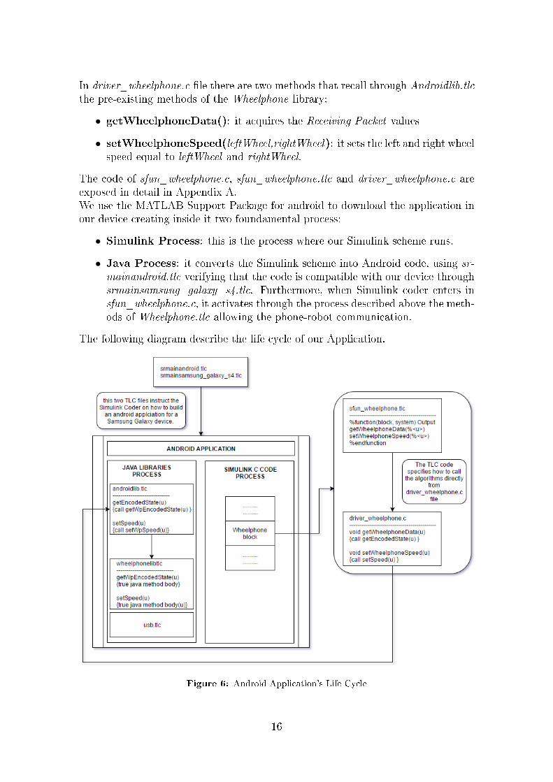
In driver_wheelphone.c �le there are two methods that recall through Androidlib.tlcthe pre-existing methods of the Wheelphone library:

• getWheelphoneData(): it acquires the Receiving Packet values

• setWheelphoneSpeed(leftWheel,rightWheel): it sets the left and right wheelspeed equal to leftWheel and rightWheel.

The code of sfun_wheelphone.c, sfun_wheelphone.tlc and driver_wheelphone.c areexposed in detail in Appendix A.We use the MATLAB Support Package for android to download the application inour device creating inside it two foundamental process:

• Simulink Process: this is the process where our Simulink scheme runs.

• Java Process: it converts the Simulink scheme into Android code, using sr-mainandroid.tlc verifying that the code is compatible with our device throughsrmainsamsung_galaxy_s4.tlc. Furthermore, when Simulink coder enters insfun_wheelphone.c, it activates through the process described above the meth-ods of Wheelphone.tlc allowing the phone-robot communication.

The following diagram describe the life cycle of our Application.

Figure 6: Android Application's Life Cycle

16

2.3 Motion Capture

Motion Capture is the process of recording the movement of objects in the threedimensional space. The interest for this topic spread among various �elds of research,from sport and entertainment, to military applications and robotics. In this Section,we want to analyze a optical Motion Capture System. It utilises data captured from

Figure 7: Optical Motion Capture System

image sensors to triangulate the 3D position and track a point of the subject in thespace between two or more cameras calibrated to provide overlapping projections.The most common approach is still the so called marker-based approach. Specialmarkers that can be easily detected through the image sensor are placed on thesubject and the information about its movements can be retrieved once a properdescription of the constraints that relate a marker to each other is deduced. Themarkers commonly used with these systems can be of two types:

• Active Markers are usually infrared LEDs placed on the subject. Ratherthen re�ecting light back that is generated externally, the markers themselvesare powered to emit their own light. These systems o�er a simpler solutionto the marker labelling problem because they allow to illuminate just onemarker at a time but of course they are more expensive since each marker isan active electronic component. The advances in computational power andthe elaboration of more sophisticated algorithms supported the widespread ofpassive motion capture systems.

• Passive Markers are coated with a retrore�ective material to re�ect theinfrared light which is generated from infrared �ash lights placed near the lensof each image sensor. An IR-pass �lter is placed above each camera so thatonly the bright re�ective markers are captured ignoring the rest of the image

17

and simplifying the marker detection problem. The centroid of the marker isestimated as a position within the two-dimensional image that is captured.

(a) Natural Light (b) Flash Light

Figure 8: Passive Markers

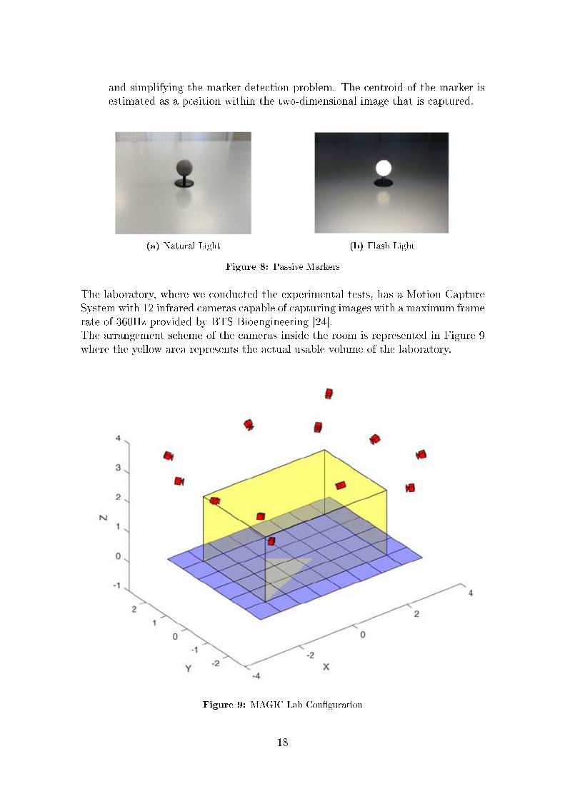
The laboratory, where we conducted the experimental tests, has a Motion CaptureSystem with 12 infrared cameras capable of capturing images with a maximum framerate of 360Hz provided by BTS Bioengineering [24].The arrangement scheme of the cameras inside the room is represented in Figure 9where the yellow area represents the actual usable volume of the laboratory.

Figure 9: MAGIC Lab Con�guration

18

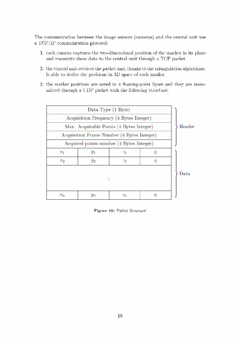
The communication between the image sensors (cameras) and the central unit usea TCP/IP communication protocol:

1. each camera captures the two-dimensional position of the marker in its planeand transmits these data to the central unit through a TCP packet

2. the central unit receives the packet and, thanks to the triangulation algorithms,is able to derive the positions in 3D space of each marker

3. the marker positions are saved in 4 �oating-point bytes and they are trans-mitted through a UDP packet with the following structure:

Figure 10: Packet Structure

19

3 The Coverage: Formulation and Algorithms

This section resumes a variety of known results in geometric optimization and inrobotic coordination. Subsection 3.1 enunciates the notion of partitions and intro-duces the multicenter function as a way to de�ne the optimal robots position in theenvironment. Subsections 3.3 and 3.4 describe two control algorithms for the agentmotion coordination and for the environment partitioning based on the classic Lloydmethod.

3.1 Voronoi Partitions, Centroids and Multicenter Function

Let X be a compact convex subset of R2 with non-empty interior. An N-partitionof X, denoted by v = (vi)

Ni=1, is an ordered collection of N subsets of X with the

following properties:

1.⋃i∈{i,...,N} vi = X;

2. int(vi)⋂int(vj) is empty for all i, j ∈ {i, ..., N} with i 6= j; and

3. each set vi, i ∈ {i, ..., N} is closed and has non-empty interior.

Let x = (x1, ..., xN) ∈ XN denote the position of N agents in the environment X.Given a group of N agents and an N -partition, each agent is one-to-one correspon-dence with a component of the partition.

Figure 11: Voronoi Partition.

The Voronoi partition W (x) of X generated by x is the ordered collection of the

21

Voronoi regions (Wi(x))Ni=1, de�ned by

Wi(x) = {q ∈ X : ‖q − xi‖ ≤ ‖q − xj‖,∀j 6= i} . (3.1)

Now, given two distinct points xi and xj in X, de�ne the (xi;xj)-bisector half-spaceby

Hbisector(xi;xj) = {q ∈ X : ‖q − xi‖ ≤ ‖q − xj‖} . (3.2)

The set Hbisector(xi;xj) is the closed half-space containing xi whose boundary isthe plane bisected by the segment from xi to xj. Note that bisector subspacessatisfy Hbisector(xi;xj) 6= Hbisector(xj;xi) and the Voronoi partition of X satis�esW (x) = X ∩ (∩j 6=iHbisector(xi;xj)).Let µ : X→ R>0 be a distribution sensory function de�ned over X. Given a genericpartition v, for each region vi, i ∈ {vi, ..., vN}, its centroid with respect to µ can beexpress as

Ci(vi) =

(∫vi

µ(q)dq

)−1 ∫vi

qµ(q)dq. (3.3)

A partition v = (v1, ..., vN) is said to be Centroidal Voronoi partition of the pair(X, µ) if

v = W (C(v)), (3.4)

i.e., v coincides with Voronoi partition generated by C(v). At the end, with thesenotations, we want to introduce the Multicer function H(v,x, µ) de�ned as

H(v,x, µ) =N∑i=1

∫vi

‖q − xi‖2µ(q)dq. (3.5)

It can be shown in [5] that, for a �xed sensory function µ, the set of local minimaof H(·,C(·), µ) coincides with the Centroidal Voronoi partitions of the pair (X, µ).

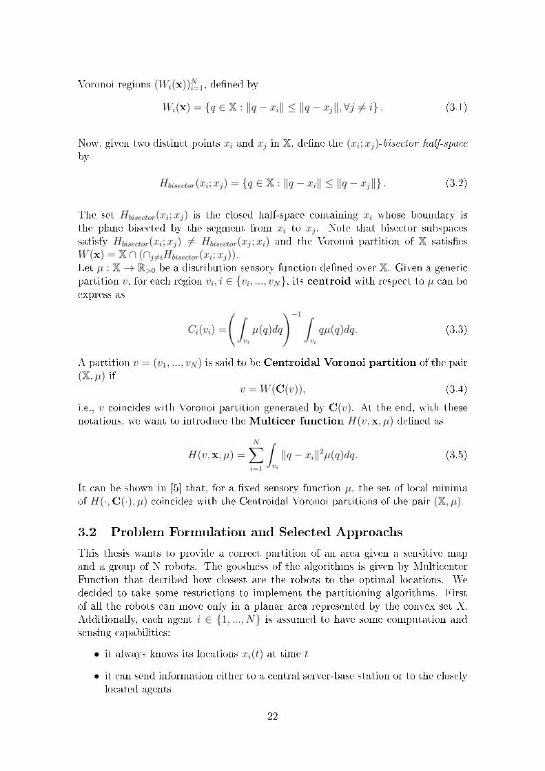
3.2 Problem Formulation and Selected Approachs

This thesis wants to provide a correct partition of an area given a sensitive mapand a group of N robots. The goodness of the algorithms is given by MulticenterFunction that decribed how closest are the robots to the optimal locations. Wedecided to take some restrictions to implement the partitioning algorithms. Firstof all the robots can move only in a planar area represented by the convex set X.Additionally, each agent i ∈ {1, ..., N} is assumed to have some computation andsensing capabilities:

• it always knows its locations xi(t) at time t

• it can send information either to a central server-base station or to the closelylocated agents

22

• it can move from its position xi,k to any desired location xi,k+1 of convex setX

As seen in Section 1.2, there are many type of partitioning methods that have uniquefeatures. In order to analyse which is the best typology for Wheelphone robots,we decided to implement two algorithms that are as di�erent from each other aspossible. The �rst algorithm is based on a synchronous client-server communicationarchitecture, instead the second one is a distribuited gossip algorithm that requiresasynchronous and pairwise communication. The next Sections describes in detailthe features of the implemented methods.

3.3 Server-based Algorithm

The �rst algorithm considered is a version of the classic Lloyd algorithm based oncentering and partitioning for the computation of Centroidal Voronoi partitions.ss

Figure 12: Client-Server Communication Architecture.

Let X ⊂ R2 be a convex and closed polygon and let µ : X→ R be a sensory function.The coverage problem is equal to �nd the partition that minimize the MulticenterFunction:

minv{H(v,C(v), µ)} . (3.6)

The Lloyd's solution for this problem is to use an iterative algorithm that can bedivided in four parts:

23

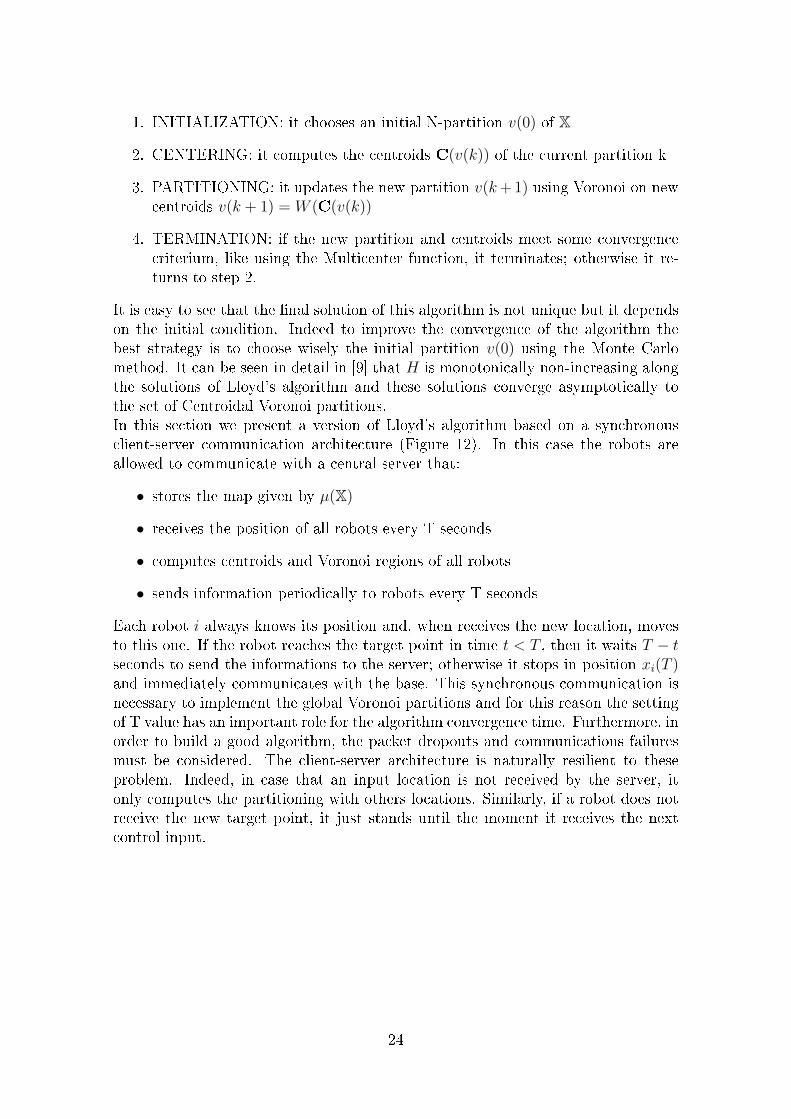
1. INITIALIZATION: it chooses an initial N-partition v(0) of X

2. CENTERING: it computes the centroids C(v(k)) of the current partition k

3. PARTITIONING: it updates the new partition v(k+ 1) using Voronoi on newcentroids v(k + 1) = W (C(v(k))

4. TERMINATION: if the new partition and centroids meet some convergencecriterium, like using the Multicenter function, it terminates; otherwise it re-turns to step 2.

It is easy to see that the �nal solution of this algorithm is not unique but it dependson the initial condition. Indeed to improve the convergence of the algorithm thebest strategy is to choose wisely the initial partition v(0) using the Monte Carlomethod. It can be seen in detail in [9] that H is monotonically non-increasing alongthe solutions of Lloyd's algorithm and these solutions converge asymptotically tothe set of Centroidal Voronoi partitions.In this section we present a version of Lloyd's algorithm based on a synchronousclient-server communication architecture (Figure 12). In this case the robots areallowed to communicate with a central server that:

• stores the map given by µ(X)

• receives the position of all robots every T seconds

• computes centroids and Voronoi regions of all robots

• sends information periodically to robots every T seconds

Each robot i always knows its position and, when receives the new location, movesto this one. If the robot reaches the target point in time t < T , then it waits T − tseconds to send the informations to the server; otherwise it stops in position xi(T )and immediately communicates with the base. This synchronous communication isnecessary to implement the global Voronoi partitions and for this reason the settingof T value has an important role for the algorithm convergence time. Furthermore, inorder to build a good algorithm, the packet dropouts and communications failuresmust be considered. The client-server architecture is naturally resilient to theseproblem. Indeed, in case that an input location is not received by the server, itonly computes the partitioning with others locations. Similarly, if a robot does notreceive the new target point, it just stands until the moment it receives the nextcontrol input.

24

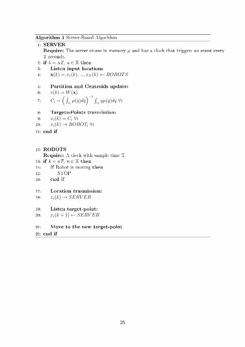
Algorithm 1 Server-Based Algorithm

1: SERVERRequire: The server stores in memory µ and has a clock that triggers an event everyT seconds.

2: if k = nT, n ∈ X then3: Listen input locations4: x(k) = x1(k), ..., xN(k) ← ROBOTS

5: Partition and Centroids update:6: v(k) = W (x)

7: Ci =( ∫

viµ(q)dq

)−1 ∫viqµ(q)dq ∀i

8: Targets-Points trasmission:9: xi(k) = Ci ∀i10: xi(k)→ ROBOTi ∀i11: end if

12: ROBOTSRequire: A clock with sample time T.

13: if k = nT, n ∈ X then14: if Robot is moving then15: STOP16: end if

17: Location trasmission:18: xi(k)→ SERV ER

19: Listen target-point:20: xi(k + 1)← SERV ER

21: Move to the new target-point

22: end if

�f

25

3.4 Distributed Gossip Algorithm

The coverage law, based upon the Lloyd algorithm and described in the previoussection, has some important limitations:

• Synchronized Communication: every T seconds each robot communicatesits position to the base station that calculates the new location,

• Base Station Presence: it must be positioned inside the range of comuni-cation signal of each vehicle. It is easy to assume that this condition can notbe veri�ed in any situation, just think of the partitioning of a very large place.

For these reasons the aim of this chapter is to introduce an distributed coveragealgorithm that reduces the communication requirements in terms of reliability, syn-chronization and topology.

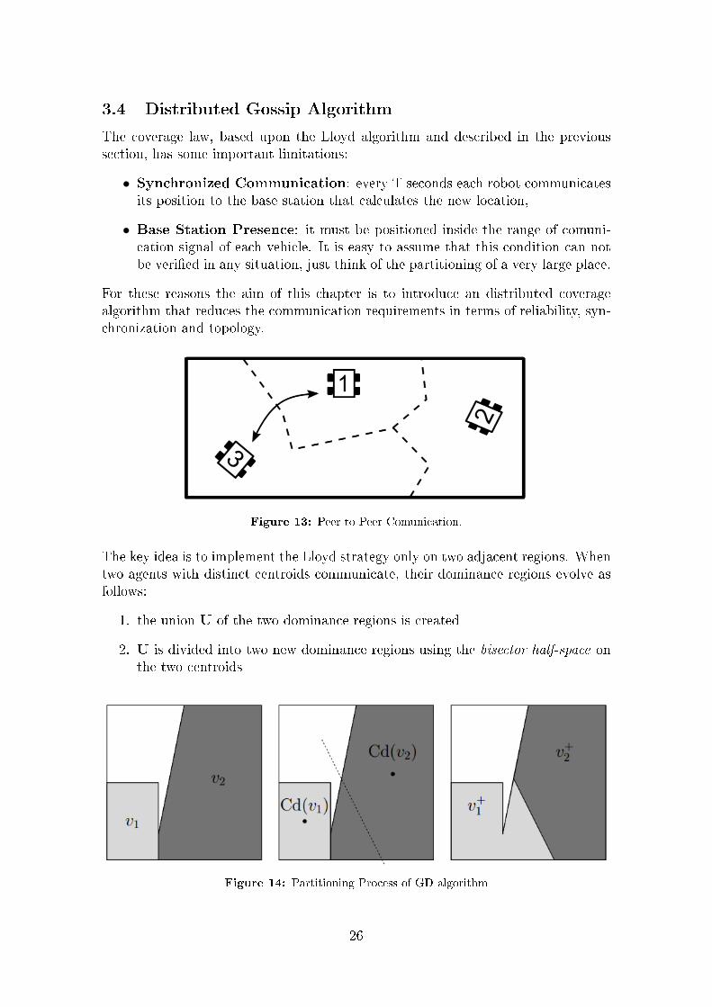
Figure 13: Peer-to-Peer Comunication.

The key idea is to implement the Lloyd strategy only on two adjacent regions. Whentwo agents with distinct centroids communicate, their dominance regions evolve asfollows:

1. the union U of the two dominance regions is created

2. U is divided into two new dominance regions using the bisector half-space onthe two centroids

Figure 14: Partitioning Process of GD algorithm

26

This idea is well-posed in the sense that the sequence of collections v(t)t∈N is anN-partition at all times t. Indeed it is immediate to see that the �rst two properties3.1 are satis�ed at all time if they are satis�ed at initial time. Finally, at all times t,each component of v(t) is closed and has non-empty interior. Indeed it is impossiblethat exist a half-plane containing the interior of a region and not containing thecentroid of the same region.The gossip coverage algorithm takes advantage of what has been said in the followingway. Let the collection (v1(0), ..., vN(0)) be an arbitrary poligonal N-partition of X.For all t ∈ N, each agent i ∈ 1, ..., N mantains in memory the dominance regionvi(t), the sensory function µ and its position xi(t). At each t ∈ N one or more pairsof distinct agents are selected by a random process. We de�ne pseudodist betweentwo closed region, va and vb, with non-empty interior:

pseudodist(va, vb) = inf {|a− b| : (a, b) ∈ int(va)× int(vb)} (3.7)

Consider i and j the two agents of a pair, they perfom the following tasks:

1. agent i transmits to agent j its dominance region vi(t) and its position xi(t)

2. agent j computes the pseudodist(vi, vj)

3. if pseudodist(vi, vj) > 0 thenthe dominance regions are not adjacent; the robots do not change their regionsand positions:

xi,j(t+ 1) = xi,j(t)

vi,j(t+ 1) = vi,j(t)

4. elsethe dominance regions are adjacent; the robots region and position change inthe following way:

vi(t+ 1) = (vi(t)⋃vj(t))

⋂Hbisector(xi(t);xj(t))

vj(t+ 1) = (vi(t)⋃vj(t))

⋂Hbisector(xj(t);xi(t))

xi(t+ 1) = Ci =( ∫

vi(t+1)µ(q)dq

)−1 ∫vi(t+1)

qµ(q)dq

xj(t+ 1) = Cj =( ∫

vj(t+1)µ(q)dq

)−1 ∫vj(t+1)

qµ(q)dq

5. agent j saves {vj(t+ 1), xj(t+ 1)} and transmits {vi(t+ 1), xi(t+ 1)} to agenti

6. agents i and j move to new positions xi(t+ 1), xj(t+ 1)

ssssIn analysing this algorithm, we observed that there is a huge problem: it can gen-erate non-convex partitions. As shown in Figure 14, that described an algorithmiteration, when the bisector half -space cuts the U region it can happen that the

27

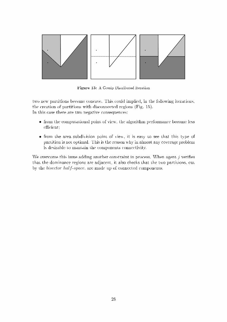
Figure 15: A Gossip Distributed Iteration

two new partitions become concave. This could implied, in the following iterations,the creation of partitions with disconnected regions (Fig. 15).In this case there are two negative consequences:

• from the computational point of view, the algorithm performance become lesse�cient;

• from the area subdivision point of view, it is easy to see that this type ofpartition is not optimal. This is the reason why in almost any coverage problemis desirable to mantain the components connectivity.

We overcome this issue adding another constraint in process. When agent j veri�esthat the dominance regions are adjacent, it also checks that the two partitions, cutby the bisector half -space, are made up of connected components.

28

4 Wheelphone Robot: modeling and control

This section describes the process that must be considered to simulate, with Simulinksoftware, the patitioning algorithms of Chapter 3.First of all, we have to create the Wheelphone object in our simulator. Subsection4.1 enunciates the kinematic and dynamic model of an unicycle robot type (that isthe same type of Wheelphone). The second fase consists in designing the motioncontol (Fig:16) that allows to drive the vehicle from one point to another.

Figure 16: Motion Control.

4.1 Unicycle Model

An unicycle type robot is, in general, a robot moving in a 2D world, having someforward speed but zero instantaneous lateral motion. In other words, it is a non-holonomic system. Despite the unicycle name, it describes vehicles having usuallytwo parallel driven wheels, each one mounted beside their center. The unicycle typerobots modeling comprises their kinematics and dynamics study, as it is usual formost the physical systems.

4.1.1 Dynamic Modeling

The dynamic modeling concerned with the study of forces and torques and theire�ect on motion, de�ning the commanding speeds. The dynamic of the vehicle is{

M dvdt

= −Kvv +Kmeam −Bvv

J dωdt

= −Kωω +Kdead −Bωω(4.1)

where v, ω are the linear and angular velocities of the vehicle, M and J are themass and the inertia of the vehicle, respectively; eam and ead are the average anddi�erential voltages applied to the wheels. Kv, Km, Kω, Kd are constant which mapforces, linear and angular velocities in forces and torques. Finally Bv and Bω arethe translational and rotational friction coe�cients, respectively.

29

The voltages applied to the wheels, VR e VL, are connected to eam e ead through{eam = 1

2(VR + VL)

ead = VR − VL(4.2)

In the end, the relation among the linear velocities of the wheels and the linear andangular velocities of the vehicle is{

vR = v + ωd

vL = v − ωd(4.3)

The dynamic of the robot has been expressed through a state-space representationusing as input the vector [eam ead]

T , as state [v ω] and, as output, the vector ofwheels velocities [vR vL]T {

x = Fx+Gu

y = Hx(4.4)

where

F =

[−Kv+Bv

M0

0 −Kω+BωJ

], G =

[KmM

00 Kd

J

]e H =

[1 d1 −d

]

4.1.2 Kinematic Modeling

Kinematics modeling describes the trajectories that mobile robots follow when theyare subject to commanding speeds. The kinematic of the vehicle is

x = 12(vL + vR) cos(θ)

y = 12(vL + vR) sin(θ)

θ = 12d

(vR − vL)

(4.5)

where x, y, θ is the pose of the vehicle, e.g. position and orientation in the plane,vR and vL are the linear speed provided by the right and left wheel, while d is thelength of the semi-axis of the vehicle.With the previous formula, it has been possible to estimate position changes overtime. The diagram (Fig: 17) shows the odometry where the three integrators areused to convert velocities x, y, θ in the vehicle pose x, y, θ.

30

Figure 17: Odometry.

4.2 Motion Control

This section describes the motion control laws which allows to drive the vehicle fromone point to another.The proposed controller exhibits a inner-outer-loop structure (Fig:16). The inner-loop control law is responsible to compute the adequate electrical signals (voltage)that will tackle the wheels's motors to force the robot to move according to a desiredlinear and angular velocity. These desired velocities are the control signals generatedby the outer-loop controller.

Figure 18: Tracking.

4.2.1 Inner-Loop

In order to drive robot to a desired linear velocity v and angular velocity ω, itis essential compute the error between the true velocities and the desired ones.Therefore, let ev and eω be respectively the linear and angular velocity errors, we

31

initially design a proportional control system{eam = −KP1ev

ead = −KP2eω(4.6)

In this case, if the dynamic of the robot has small static gains, the velocities errorsmay remain signi�cant. Then, adding an integral term, we can enforce the steadystate error convergence to zero.{

eam = −KP1ev −KI1

∫ t0ev(τ)dτ

ead = −KP2eω −KI2

∫ t0eω(τ)dτ

(4.7)

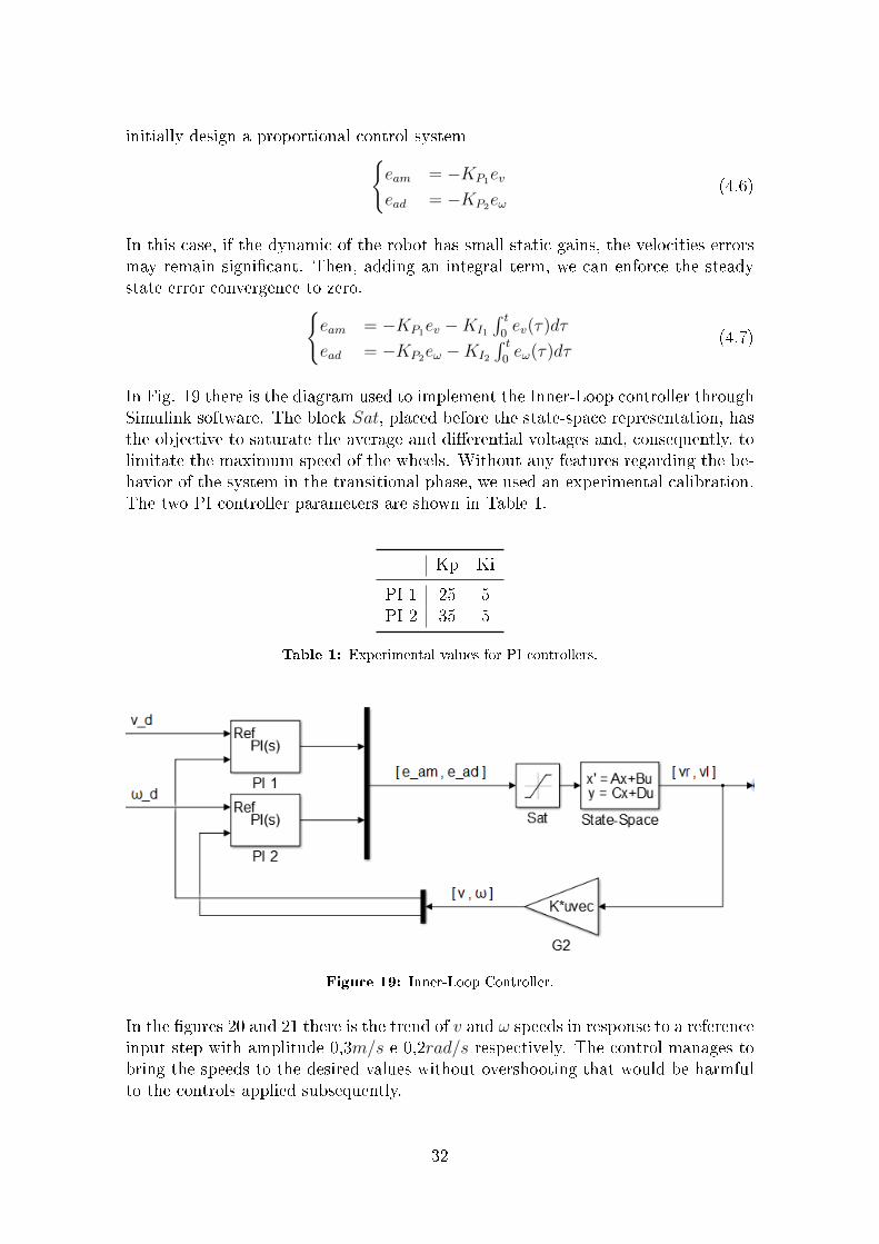
In Fig. 19 there is the diagram used to implement the Inner-Loop controller throughSimulink software. The block Sat, placed before the state-space representation, hasthe objective to saturate the average and di�erential voltages and, consequently, tolimitate the maximum speed of the wheels. Without any features regarding the be-havior of the system in the transitional phase, we used an experimental calibration.The two PI controller parameters are shown in Table 1.

Kp Ki

PI 1 25 5PI 2 35 5

Table 1: Experimental values for PI controllers.

Figure 19: Inner-Loop Controller.

In the �gures 20 and 21 there is the trend of v and ω speeds in response to a referenceinput step with amplitude 0,3m/s e 0,2rad/s respectively. The control manages tobring the speeds to the desired values without overshooting that would be harmfulto the controls applied subsequently.

32

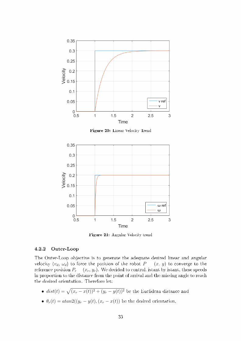
Figure 20: Linear Velocity Trend

Figure 21: Angular Velocity trend

4.2.2 Outer-Loop

The Outer-Loop objective is to generate the adequate desired linear and angularvelocity (vd, ωd) to force the position of the robot P = (x, y) to converge to thereference position Pr = (xr, yr). We decided to control, istant by istant, these speedsin proportion to the distance from the point of arrival and the missing angle to reachthe desired orientation. Therefore let:

• dist(t) =√

(xr − x(t))2 + (yr − y(t))2 be the Euclidean distance and

• θr(t) = atan2((yr − y(t), (xr − x(t)) be the desired orientation,

33

the contro law is

vd = Kvdist(t)

ωd = Kω(θd(t) θ(t))(4.8)

where Kv and Kω are the controller parameters and the operator computes thedi�erence between the angles expressed as a value between −π and π.For the same reason of paragraph 4.2.1, we used an experimental calibration todetermine Kv and Kω that are:

Kv = 4 Kω = 9.

The most important value that we have to de�ne is Kω. Indeed faster the robot�nds the right direction less path it will take. The �gure 22 exhibits the trajectorythat the controller makes the robot do to reach the position (-0.5,0.5). As we cansee, it starts from the origin with an initial orientation equal to the one of the x-axisuntill it gets to the target.

Figure 22: A Vehicle Trajectory

ssThe diagram in Fig. 23 is the Outer-Loop implementation in Simulink softwarewhere the Inner-Loop and Odometry blocks are the same used in Fig. 19 and Fig.17.

34

Figure 23: Outer-Loop.

The hypot and atan2 blocks are provided by Simulink performing the followyngmath operation:

• hypot(x, y) =√x2 + y2

• atan2(x, y) = arctan(xy)

The F1 block, instead, is a function built by us, through MATLAB function block,to perfom the operator. In the next lines it is shown the F1 code

Algorithm 2 F1 function

1: function theta1 = F1(theta)

2: while theta > π do3: theta = theta−2π;

4: end

5: while theta < −π do6: theta = theta+2π;

7: end

8: theta1 = theta;

The process until here described, composed by:

• unicycle dynamic

• unicycle kinematic

• inner-loop controller

• outer-loop controller,

has allowed us to create a robot simulator whereby we tested the partitioning al-gorithms in a simulated environment before implementing them on real devices.These tests have improved the debugging phase of the algorithms letting us be moree�cient in the experimental stage.

35

sss

36

5 Numerical and Experimental Results

This section presents in detail the steps performed in the MagicLab laboratoryof Padova's engineering department to implement the partitioning algorithms onWheelphone devices. It is organized in the following setting:

• we provide the features of the preliminary diagrams used to perform motioncontrol and its results

• we introduce the algorithms created for the reconstruction of the vehicles poseshaving access to the data obtained from the Motion Capture System of Section2.3

• we show how we implemented the Server-Based algorithm and the DistributedGossip algorithm in MATLAB Simulink.

• �nally, we show some real simulations of the two algorithms chosen in Section3.

5.1 Preliminary Results

Before testing the validity of partitioning algorithms, we must make sure that themotion control, designed in a simulated environment, is also robust with real devices.Then we installed in our smartphone an Application that contained the Simulinkdiagram of Figure 24.The ODOMETRY and the MOTION CONTROLLER blocks have the same struc-ture as those presented respectively in sections 4.1.2 and 4.2.2 while we replaced theinner-loop block with sfun_wheelphone as it is no longer necessary to simulate therobot dynamics. Since the S-function inputs, vL and vR, i.e. left and right wheel

Figure 24: Application Simulink Scheme

speeds, are di�erent from the Motion Controller outpus, v and ω, i.e. linear andangular robot speeds, we included in the control chain a matrix gain H to performthe conversion of the values:

H =

[1 1d −d

]37

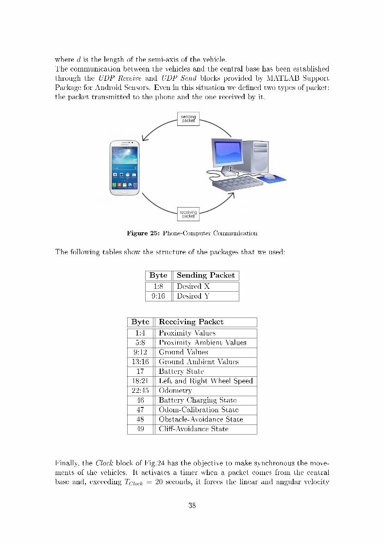
where d is the length of the semi-axis of the vehicle.The communication between the vehicles and the central base has been establishedthrough the UDP Receive and UDP Send blocks provided by MATLAB SupportPackage for Android Sensors. Even in this situation we de�ned two types of packet:the packet transmitted to the phone and the one received by it.

Figure 25: Phone-Computer Communication

The following tables show the structure of the packages that we used:

Byte Sending Packet

1:8 Desired X9:16 Desired Y

��

Byte Receiving Packet

1:4 Proximity Values5:8 Proximity Ambient Values9:12 Ground Values13:16 Ground Ambient Values17 Battery State

18:21 Left and Right Wheel Speed22:45 Odometry46 Battery Charging State47 Odom-Calibration State48 Obstacle-Avoidance State49 Cli�-Avoidance State

�

Finally, the Clock block of Fig.24 has the objective to make synchronous the move-ments of the vehicles. It activates a timer when a packet comes from the centralbase and, exceeding TClock = 20 seconds, it forces the linear and angular velocity

38

equal to zero. We chose to make synchronous the movement of the robots and nottheir communication because creating independent clocks in the vehicles and in thebase station could lead to asynchronous communications implyng control failure.�Applying the above scheme through a huge number of experimental tests, we cali-brated the proportional constants, Kv and Kω, of the motion controller, obtainingthe following values:

Kv = 2 Kω = 5.

Nevertheless we faced that in same cases the vehicle did not reach the desired �nalposition. In fact, placing the robot with a speci�c orientation and choosing as a�nal point a destination distant at least 2 meters and that is exactly in the oppositedirection, the vehicle instead of steering mantains the initial orientation. This iscaused by the presence of internal saturators in the two robot motors that limit themaximum wheels speed. In these situation, being our motion control proportional tothe distance, the velocity of the left and the right wheels would exceed the saturatorsthreshold and, not being possible, they are set equal to the threshold itself. Tosolve this problem, we primarly reduced the Kv value realizing that also the vehicleperformance was lowered in the short-distance trips. For this reason we opted toinsert a saturator in the Motion Controller with the scope to limit the linear velocityto the 80% of the threshold. In this way, even if the robot potentialities are underexploited, the motion control is working equally for all range of distance.

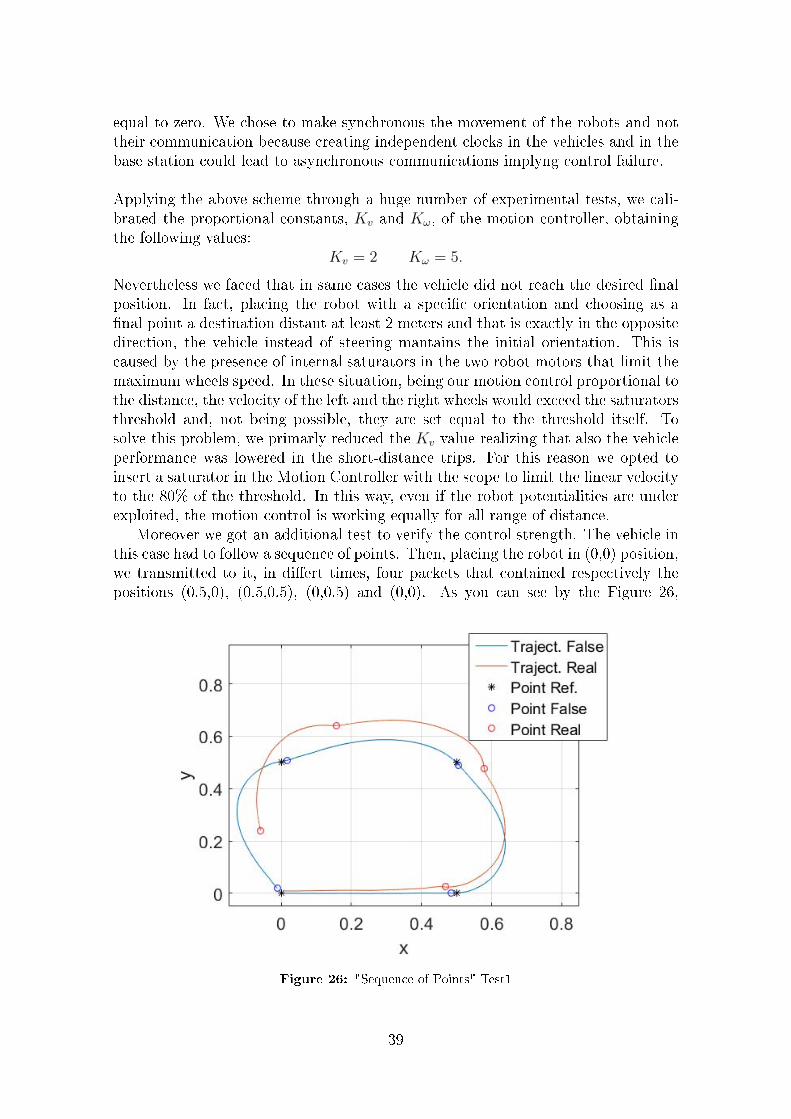
Moreover we got an additional test to verify the control strength. The vehicle inthis case had to follow a sequence of points. Then, placing the robot in (0,0) position,we transmitted to it, in di�ert times, four packets that contained respectively thepositions (0.5,0), (0.5,0.5), (0,0.5) and (0,0). As you can see by the Figure 26,

Figure 26: "Sequence of Points" Test1

39

the trajectory and the places where it stopped are di�erent from those in whichit thought to be. This anomaly could be caused by the lack of the encoders thatmeasure the actual speed of the motors. In fact, using the counter-electromotiveforce, the engine speed in our device is only estimated. Being that an intrinsicproblem, is not possible to solve it through a software reprogramming and for thisreason we chose to adopt the Motion Capture System described in Section 2.3. Inthe following subsection is explain in more detail the use of the Motion CaptureSystem in our application.

5.2 Pose Reconstruction with 3D Motion Capture System

In the section 2.3 we analized the modality which the Motion Capture System ac-quires the markers position. The purpose of this chapter, instead, is to obtain theWheelphones pose, i.e. position and orientation in the three-dimensional space, frommarkers data.We choose to link each robot to a pattern of 4 markers since that one single markergives us only three degrees of freedom which represent its position but no informationabout the orientation of the reference frame attached to it. To do this, we removedthe upper case installing a cardboard with the markers as you can see in Figure 27.Before explaining how the robots pose is rebuilt, it is necessary to understand how

Figure 27: Wheelphone Robot with Markers

we make the markers labelling in order to connect each marker to the right pattern.The following subsection will describe the structure of the used algorithm.ss

5.2.1 Marker Labelling

Multiple markers are non distinguishable from a camera point of view, there areno distinctive parameters intrinsic to the marker such as colour or shape, they alllook as bright elliptic blobs, whose position is later approximated by their centroid.

40

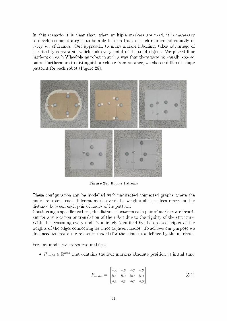
In this scenario it is clear that, when multiple markers are used, it is necessaryto develop some strategies to be able to keep track of each marker individually inevery set of frames. Our approach, to make marker labelling, takes advantage ofthe rigidity constraints which link every point of the solid object. We placed fourmarkers on each Wheelphone robot in such a way that there were no equally spacedpairs. Furthermore to distinguish a vehicle from another, we choose di�erent shapepatterns for each robot (Figure 28).ss

Figure 28: Robots Patterns

These con�guration can be modelled with undirected connected graphs where thenodes represent each di�erent marker and the weights of the edges represent thedistance between each pair of nodes of its pattern.Considering a speci�c pattern, the distances between each pair of markers are invari-ant for any rotation or translation of the robot due to the rigidity of the structure.With this reasoning every node is uniquely identi�ed by the ordered triplet of theweights of the edges connecting its three adjacent nodes. To achieve our purpose we�rst need to create the reference models for the structures de�ned by the markers.

For any model we stores two matrices:

• Pmodel ∈ R3×4 that contains the four markers absolute position at initial timess

Pmodel =

xA xB xC xDyA yB yC yDzA zB zC zD

(5.1)

41

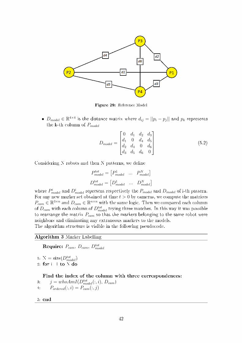
Figure 29: Reference Model

• Dmodel ∈ R4×4 is the distance matrix where dij = ||pi − pj|| and pk representsthe k-th column of Pmodel

Dmodel =

0 d1 d2 d3d1 0 d4 d5d2 d4 0 d6d3 d5 d6 0

(5.2)

Considering N robots and then N patterns, we de�ne

P totmodel =

[P 1model ... PN

model

]Dtotmodel =

[D1model ... DN

model

]where P i

model and Dimodel represent respectively the Pmodel and Dmodel of i-th pattern.

For any new marker set obtained at time t > 0 by cameras, we compute the matricesPcam ∈ R3×n and Dcam ∈ Rn×n with the same logic. Then we compared each columnof Dcam with each column of Dtot

model trying three matches. In this way it was possibleto rearrange the matrix Pcam so that the markers belonging to the same robot wereneighbors and eliminating any extraneous markers to the models.The algorithm structure is visible in the following pseudocode.

Algorithm 3 Marker Labelling

Require: Pcam, Dcam, Dtotmodel

1: N = size(Dtotmodel)

2: for i=1 to N do

Find the index of the column with three correspondences:3: j = whoAmI(Dtot

model(:, i), Dcam)4: Pordered(:, i) = Pcam(:, j)

5: end

42

5.2.2 Pose Reconstruction

Obtained the correspondence between the initial models and each set of points att > 0, we want to implement an algorithm that reconstructs the Wheelphones poses.It is important to underline that, since we need just three points to compute theposition and orientation of one vehicle in 3D space, using more markers improve thealgorithm robustness in case of one or more misdetections.The pose reconstruction of any robot was connected to a least squares problem.Indeed, let P =

[p1 p2 ... pn

]and Q =

[q1 q2 ... qn

]be two di�erent sets of

points, to �nd Wheelphone pose is equal to �nd the matrices R ∈ SO(3), rotationmatrix, and T, translation vector, that solve the following formula:

(R, T ) = arg minR,T

n∑i=1

||(Rpi + T )− qi||2 (5.3)

Following the reasoning described in [25], let R and T be the two solution of (5.3),then Q and Q′ = RQ have the same centroid:

cQ ≡ cQ′

where cQ and cQ′ represent rispectively the controid of Q and Q′.Therefore, it is possible to divide the least squares problem into two equations toderive the matrices R and T :

• R = arg minR Σ2 = arg minR∑n

i=1 ||h′i −Rhi||2

• T = cQ − cP

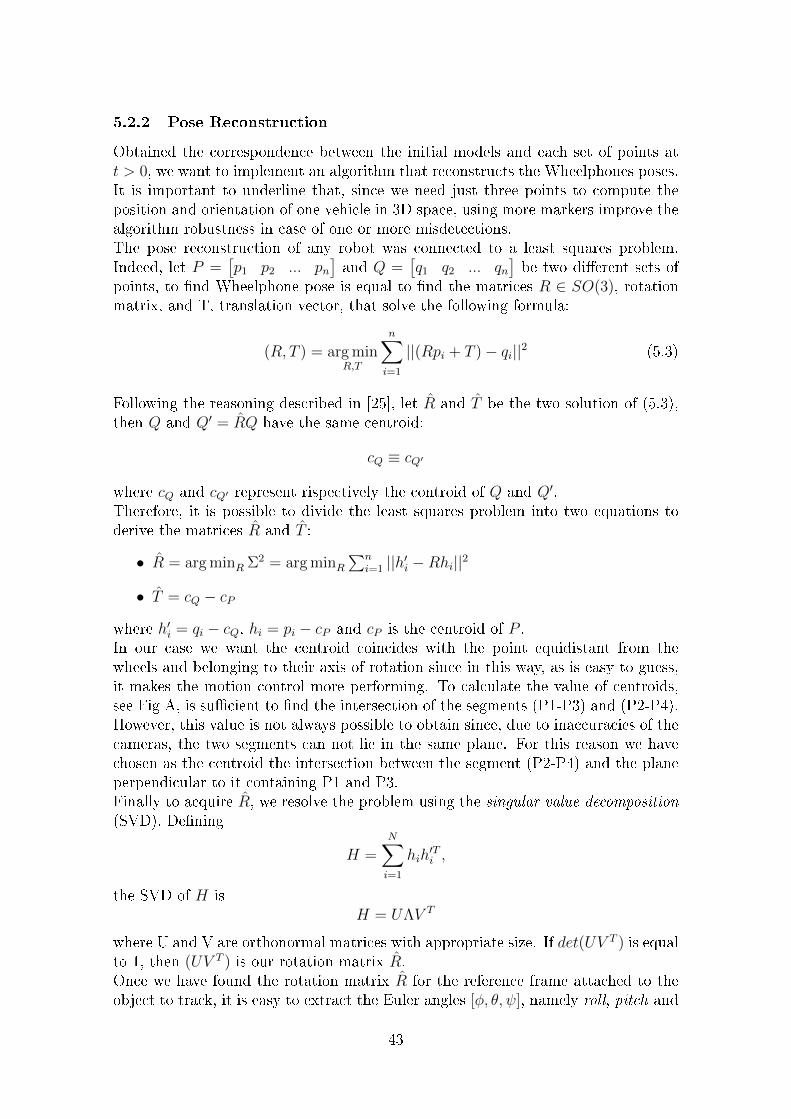
where h′i = qi − cQ, hi = pi − cP and cP is the centroid of P .In our case we want the centroid coincides with the point equidistant from thewheels and belonging to their axis of rotation since in this way, as is easy to guess,it makes the motion control more performing. To calculate the value of centroids,see Fig A, is su�cient to �nd the intersection of the segments (P1-P3) and (P2-P4).However, this value is not always possible to obtain since, due to inaccuracies of thecameras, the two segments can not lie in the same plane. For this reason we havechosen as the centroid the intersection between the segment (P2-P4) and the planeperpendicular to it containing P1 and P3.Finally to acquire R, we resolve the problem using the singular value decomposition(SVD). De�ning

H =N∑i=1

hih′Ti ,

the SVD of H isH = UΛV T

where U and V are orthonormal matrices with appropriate size. If det(UV T ) is equalto 1, then (UV T ) is our rotation matrix R.Once we have found the rotation matrix R for the reference frame attached to theobject to track, it is easy to extract the Euler angles [φ, θ, ψ], namely roll, pitch and

43

yaw, which express the rotation along the x, y and z axis. The rotation matrix canbe rewritten as follows:

R =

cθcψ − sφsψsθ −sψcφ cθsφcψ + cψsθcθsψ + cψsφsθ cψcφ sψsθ − cψsφcθ−cφsθ sφ cθcφ

which leads to the following relations:

ψ = Atan2(−r12, r22)

φ = Atan2(r32,

√r231 + r233

)θ = Atan2(−r31, r33)

where φ belongs to the interval (−π/2, π/2).In our case, φ and ψ are always zero since the only rotation that the robot canperform is around its z axis. Indeed only θ describes the orientation of the vehicleand for this it is the only angle considered for our experiments.

5.2.3 Implementation

We con�gured the motion capture system to work with Simulink using the followingblock scheme:

Figure 30: Simulink Motion Capture Block Scheme

The Packet Input block receives the packets with the structure of Figure 10 and,through Bytes Array to Floats function, derives the spatial coordinates of eachmarker. The blue and green blocks implement sequentially the algorithms of Mark-ers Labelling and Pose Reconstruction described in the previous sections.This scheme is performed by the Central-Base which must, in addition to send thereference positions, transmit the actual locations of vehicles moment for moment.Moreover we repeated the test of Section 6.1 in which the robot tried to follow asequence of points. In Figure 31 we compared the real trajectories and the realplaces where the vehicle stopped using two di�erent motion control:

• Trajectory1 and Point1 are produced by the control utilizing the wheelsodometry,

44

• Trajectory2 andPoint2 refer to the control implemented through the MotionCapture System.

As we can see, the second one is much more accurate detecting a maximum posi-tioning error equal to 2 cm.For this reason, the experimental results which will be shown in section 5.4, areobtained using only the motion control implemented through the Motion CaptureSystem.

Figure 31: "Sequence of Points" Test2

45

5.3 Coverage Algorithms Simulations

In this section we want to exhibit how we implemented the partitioning algorithmsin MATLAB sofware using the previously described motion control.We consider a team of N robots and a squared domain X = [0, 2]×[0, 2]. The sensoryfunction µ(x) is a combination of two bi-dimensional Gaussians:

µ(x) = e−‖x−µ1‖

2

0.0313 + 2e−‖x−µ2‖

2

0.125 (5.4)

where the Gaussian centers are located in position µ1 = [0.675, 0.675] and µ2 =[1.625, 1.425]. This function is shown in Fig. 32 in three-dimensional space.

Figure 32: Gaussian Sensory Function

Successively, to use µ(x) in our algorithms, we represented it as a square matrix Iof size equal to 500×500 where I(i, j) = µ([xj, yi]). We de�ne

ki2m =2 meters

500 index= 0, 004

as the costant that convert the indexs of I in meters{yi = ki2mi

xj = ki2mj(5.5)

The matrix size is an important value that has to be calibrated because a highervalue implies that the Gaussians are more accurately discretized while a lower oneinvolves an improvement of the computation time.The �gure 33 shows the matrix I in a grayscale image where the white color isassociated with higher values of µ while black with the lower ones.This matrix is the map on which we apply the two partitioning algorithms.

46

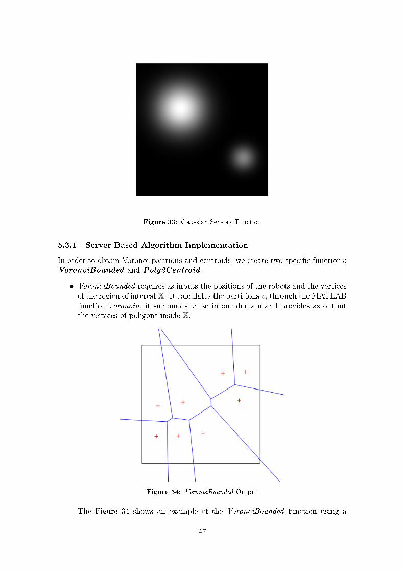
Figure 33: Gaussian Sensory Function

5.3.1 Server-Based Algorithm Implementation

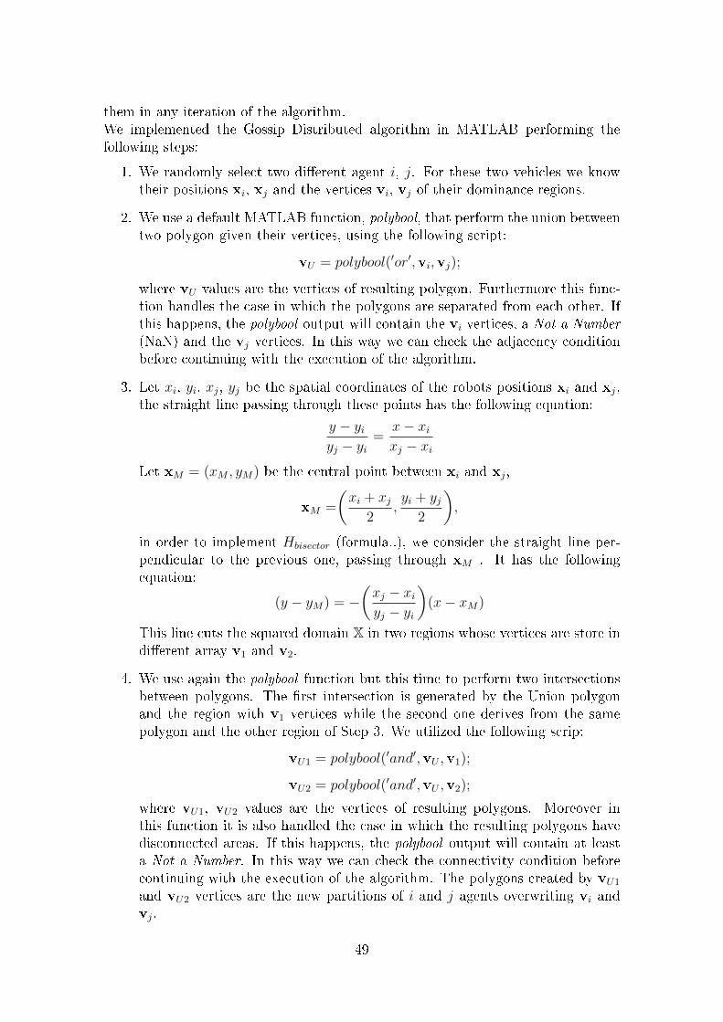
In order to obtain Voronoi paritions and centroids, we create two speci�c functions:VoronoiBounded and Poly2Centroid .

• VoronoiBounded requires as inputs the positions of the robots and the verticesof the region of interest X. It calculates the partitions vi through the MATLABfunction voronoin, it surrounds these in our domain and provides as outputthe vertices of poligons inside X. ss

Figure 34: VoronoiBounded Output

The Figure 34 shows an example of the VoronoiBounded function using a

47

team of 8 robots arranged in a random way. The black and the blue linesrepresent respectively the boundaries of our domain and those of voronoinfunction generated by the robots position (red cross).

• Poly2Centroid requires as inputs the vertices of a polygon and the matrix Ithat described the sensory function µ. It considers only the values of I insidethe polygon, calculates the centroid throgh the formula 3.3 and provides asoutput the coordinates cx and cy of the point. ss

Figure 35: Poly2Centroid Output

The Figure 35 displays an example of Poly2Centroid function. Using thevertices of the upper left partition of Fig.34 it cuts out the sensory functioncomputing its centroid (green circle).

To use both functions in MATLAB, we installed the Mapping Toolbox that providesalgorithms for performing operations on polygons.Setting the values of cx and cy as "Desired X " and "Desired Y ", the server basetrasmits them to phone moving the vehicle to the centroid of its partition. Finallythis process "partitioning, centering and moving" was performed iteratively severaltimes. The Server-Based results are exposed in section 5.4.

5.3.2 Gossip Distributed Algorithm Implementation

The Gossip Distributed algorithm requires that, through a communication network,the robots theirself store and calculate their partition without an external sourcewhich oversees the process. This idea is inconsistent with our situation because isthe central base the one who calculates where the vehicles are located in the plane.Without it the motion control, that is the basis of our partitioning algorithm, wouldbe impossible to implement. Furthermore, if we left to the vehicles deciding whenand to whom to transmit, many communication issues, for example the packetscollision, would be managed.For these reasons we chose to simulate the distributed feature through a centralbase. The central server knows each robots partition but it considers only two of

48

them in any iteration of the algorithm.We implemented the Gossip Distributed algorithm in MATLAB performing thefollowing steps:

1. We randomly select two di�erent agent i, j. For these two vehicles we knowtheir positions xi, xj and the vertices vi, vj of their dominance regions.

2. We use a default MATLAB function, polybool, that perform the union betweentwo polygon given their vertices, using the following script:

vU = polybool(′or′,vi,vj);

where vU values are the vertices of resulting polygon. Furthermore this func-tion handles the case in which the polygons are separated from each other. Ifthis happens, the polybool output will contain the vi vertices, a Not a Number(NaN) and the vj vertices. In this way we can check the adjacency conditionbefore continuing with the execution of the algorithm.

3. Let xi, yi, xj, yj be the spatial coordinates of the robots positions xi and xj,the straight line passing through these points has the following equation:

y − yiyj − yi

=x− xixj − xi

Let xM = (xM , yM) be the central point between xi and xj,

xM =

(xi + xj

2,yi + yj

2

),

in order to implement Hbisector (formula..), we consider the straight line per-pendicular to the previous one, passing through xM . It has the followingequation:

(y − yM) = −(xj − xiyj − yi

)(x− xM)

This line cuts the squared domain X in two regions whose vertices are store indi�erent array v1 and v2.

4. We use again the polybool function but this time to perform two intersectionsbetween polygons. The �rst intersection is generated by the Union polygonand the region with v1 vertices while the second one derives from the samepolygon and the other region of Step 3. We utilized the following scrip:

vU1 = polybool(′and′,vU ,v1);

vU2 = polybool(′and′,vU ,v2);

where vU1, vU2 values are the vertices of resulting polygons. Moreover inthis function it is also handled the case in which the resulting polygons havedisconnected areas. If this happens, the polybool output will contain at leasta Not a Number. In this way we can check the connectivity condition beforecontinuing with the execution of the algorithm. The polygons created by vU1

and vU2 vertices are the new partitions of i and j agents overwriting vi andvj.

49

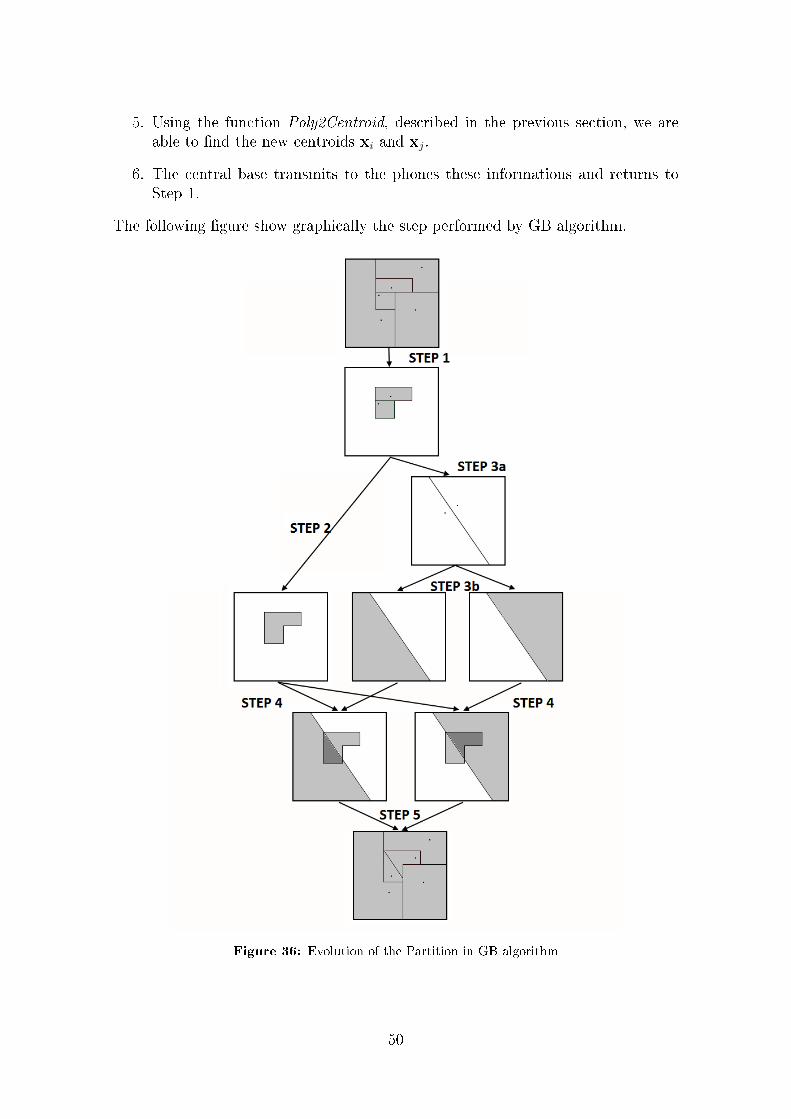
5. Using the function Poly2Centroid, described in the previous section, we areable to �nd the new centroids xi and xj.

6. The central base transmits to the phones these informations and returns toStep 1.

The following �gure show graphically the step performed by GB algorithm.

Figure 36: Evolution of the Partition in GB algorithm

ss

50

5.4 Results

In this section we show the results obtained by the Server Based and Gossip Dis-tributed algorithms. They are implemented both on ideal unicycles vehicles andwheelphones devices. In the �rst case we used the motion control based on theresults given by the wheels odometry. In the other case the motion control designedwas based on the information resulting from the Motion Capture System.To compare the four experiments we decided to use the same initial conditions(Fig.37):

• 5 robots: four vehicles positioned in the corners of the squared domain andone located in the central point

• Partitions: the dominance region of each agent is the Voronoid partitiongiven by the initial positions of the robots

• Map: the sensory function µ described in Section 5.3.

Figure 37: Initial conditions.

Each algorithm was processed 40 times and for each iteration the central serverstored the values of the vehicles position and the boundary of their partitions. Inthe following �gures are shown some of the 40 iterations, speci�cally the numbers 1,5, 20 and 40. Since for each algorithm we made two experiments, the �gures thatwe obtained are four. Figures 38 and 39 refer to the Server Based approach, while�gures 40 and 41 relate to the Gossip Distributed proces.

51

Figure 38: Evolution of Simulate Server Based Algorithm

52

Figure 39: Evolution of Experimental Server Based Algorithm

53

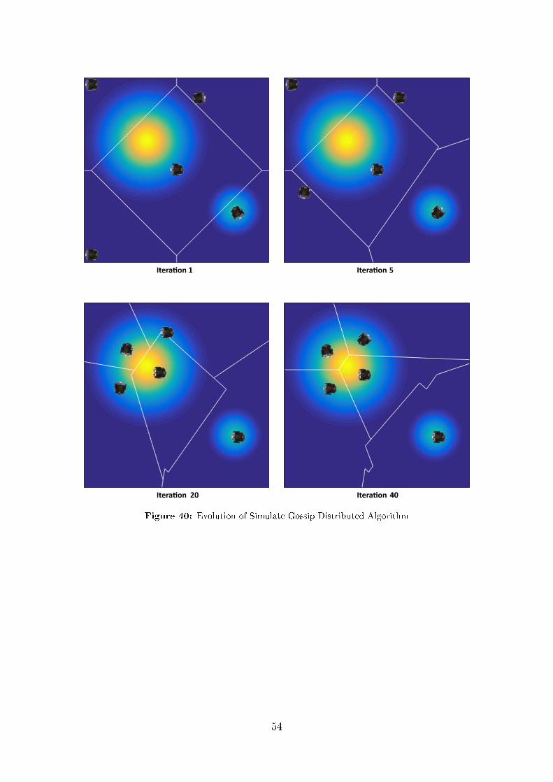
Figure 40: Evolution of Simulate Gossip Distributed Algorithm

54

Figure 41: Evolution of Experimental Gossip Distributed Algorithm

55

As it is possible to see, for all the four experiments the �nal positions are almostthe same: four robots surrond the most critical area (the yellow zone) while theremaining vehicle stand on the less critical one. This result re�ects our expectationssince the sensory function is generated by the union of two Gaussian that have onethe twice amplitude respect to the other. Hence the most important zone have tobe monitored by more robots than the other area. Moreover, considering that eachiteration is depending on the previous one and the initial condition is the same forall the experiments, it was predictable that the �nal positions were similar.Analysing the partitions, we can see that there is a di�erence between the ServerBased approach and the Gossip Distributed one. In the �rst case there are alwaysconvex partitions with a low number of vertices and simply shapes. This is dueto the global characteristic of the algorithm which obtain the dominance regionsstudying all the agents position. In the second case we can �nd concave partitionswith complicated shapes. This is caused by pairwise comunications between agents,in fact if two robots do not interact for many interations, the boundary betweentheir partitions can be a jagged line. In our case, since the number of robots used issmall, this problem have not a�ected the algorithm performances. In situations witha huge number of agents, it is advisable to not choose randomly the two robots thathave to communicate, but to select them following speci�c criteria like, for example,by increasing the communication possibility between vehicles with several verticespartition.

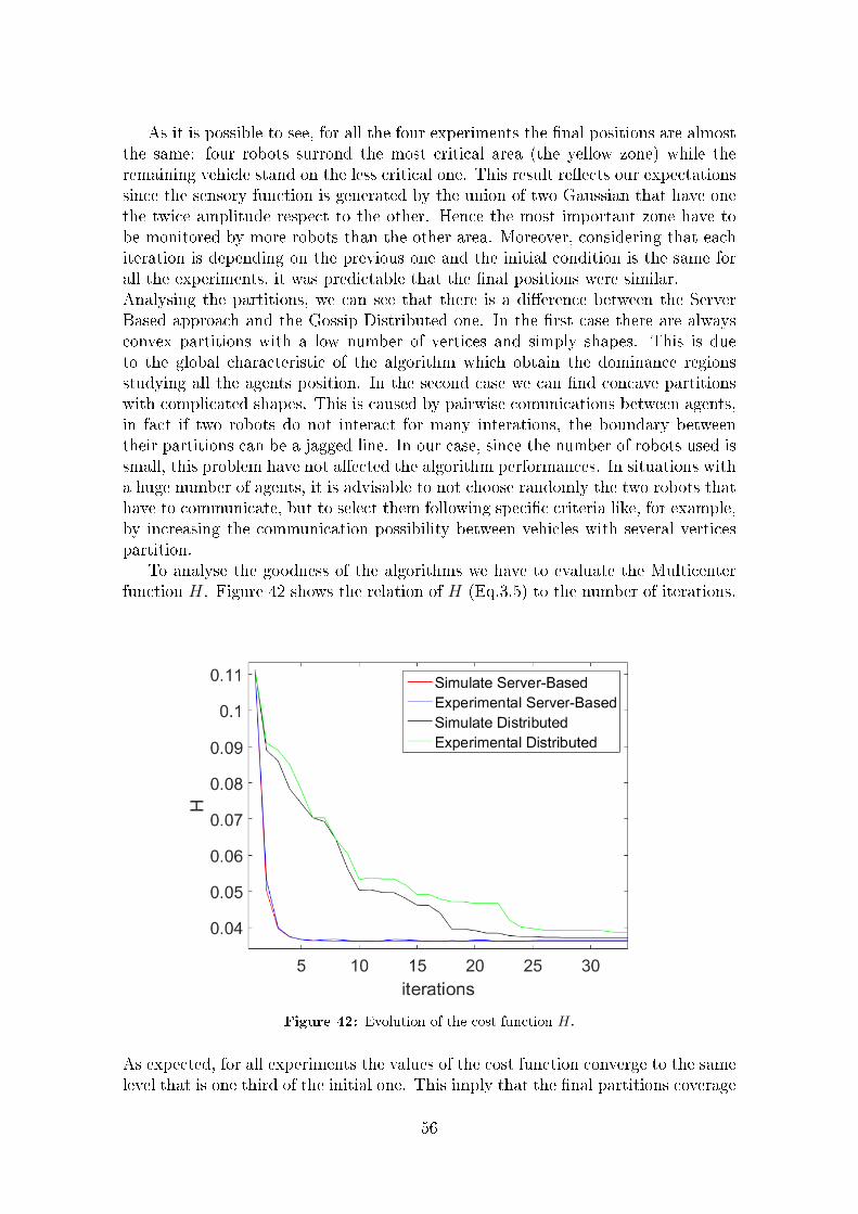
To analyse the goodness of the algorithms we have to evaluate the Multicenterfunction H. Figure 42 shows the relation of H (Eq.3.5) to the number of iterations.ss

Figure 42: Evolution of the cost function H.

As expected, for all experiments the values of the cost function converge to the samelevel that is one third of the initial one. This imply that the �nal partitions coverage

56

the domain more e�ciently than the initial conditions. Furthermore, since the SBand GD algorithms are based on the classical method of Lloyd, H is characterizedby a non-increasing behavior.Evaluating now the convergence rate of the function, we can see how the ServerBased algorithm is faster than the Gossip Distributed one. This di�erence is at-tributed again to the di�erent approach of the algorithms. In the �rst case all thevehicles are always involved in any iteration while in the second one only two ofthem.Finally we can note a worsening performance in the experiments where we usedreal devices respect to ideal ones. This is caused by the di�erent accuracy of themotion control. In the ideal case the robots are in the precise locations where thepartitioning algorithms commanded to stand. Instead, implementing the control onreal devices, although we utilized the Motion Capture System, there were alwayssmall positioning errors.

57

6 Conclusions

In this work two partitioning algorithms were implemented on Wheelphones devicesin order to coverage optimally a speci�c area. We ran this process through an Ap-plication for smartphones enhancing the traditional coverage methods.After a brief introduction on the importance that this technology is assuming in theseyears, we described the pre-existing hardware and software features of a Wheelphonerobot. Thanks to them and the Support Package for Android of MATLAB, we wereable to build a custom S-Function block in Simulink in order to handle the low-levelcommunication between the robot and the smartphone. This step has been crucialfor the success of our implementation as it allowed us to program with a high-levellanguage enabling a faster addition or change of the control components.Successively we exposed the geometric concepts of Voroid partition and centroid usedby classic Lloyd method in order to �nd the optimal area partition. The algorithmsproposed in this thesis were two versions of this method with di�erent communica-tion architecture. The �rst one employed a centralized approach where each agenthave to communicate only its position to a central server in a synchronous manner.Afterwards, this server calculates the new partitions and positions retransmittingthem to the vehicles. The second algorithm followed a distributed method whereonly two agents are involved in any iteration. In this case the vehicles themselveshave to compute the information about their partitions and positions.Later we provided the mathematical model for an unicycle vehicle that is the sametype of Wheelphone robot. Studing its dynamic and kinematic we created a simplemotion control that allowed us to drive the vehicle from one point to another.Finally we showed the work made in laboratory on Wheelphone devices. Beforethat it was necessary to implement the Marker Labelling and Pose Reconstractionalgorithms essential to estimate the positions and orientations of the robots.On the basis of the results obtained, we veri�ed the right functioning of the algo-rithms succeeding in minimizing the Multicenter Function H in 5 and 35 iterationsrespectively for the Server Based algorithm and the Gossip Distributed one.

Many future developments can be led at each level of the proposed work. From atheorical point of view can be tested more complex partitioning algorithms includinga non convex enviroment with obstacles presence and time-varying density functions.Then it is possible to exploit the phone and Wheelphone sensors, like camera, I-Rand ambient sensors. In this way the robots themselves can estimate the map thathas to be covered. In this regard we suggest the implentation of the algorithms of[22] where the map estimation phase and the coverage one are simultaneoisly ran.Furthermore can be designed a more robust and reliable motion control. In additionto moving the robots from one point to another, it has to decide which trajectorythey have to follow. In this way the vehicles can avoid the other agents or obstaclespresent in the area. Finally from the pratical point of view, can be installed onWheelphone two motors encoders in order to know exactly the angular positionsof the wheels. Managing the low-level communication, the Motion Control can beindipendent from the Motion Capture System of the laboratory making robots ableto act in all type of environment.

59

7 APPENDIX

A Wheelphone Drivers

A.1 sfun_wheelphone.c

#define S_FUNCTION_NAME sfun_wheelphone

#define S_FUNCTION_LEVEL 2

#include "simstruc.h"

#define NUM_INPUTS 1

#define NUM_OUTPUTS 11

#define NUM_PARAMS 0

#define NUM_CONT_STATES 0

#define NUM_DISC_STATES 0

#define SAMPLE_TIME_0 INHERITED_SAMPLE_TIME

/* Input Port 0 (Left/right speed ref) */

#define INPUT_0_WIDTH 2

#define INPUT_0_DTYPE SS_INT32

#define INPUT_0_COMPLEX COMPLEX_NO

#define INPUT_0_FEEDTHROUGH 1

/* Output Port 0 (front proximity sensors) */

#define OUTPUT_0_WIDTH 4

#define OUTPUT_0_DTYPE SS_UINT8

#define OUTPUT_0_COMPLEX COMPLEX_NO

/* Output Port 1 (front ambient sensors) */




/* Output Port 2 (ground proximity sensors) */




/* Output Port 3 (ground ambient sensors) */




/* Output Port 4 (battery charge [%]) */




/* Output Port 5 (estimated left/right speed [mm/s]) */


#define OUTPUT_5_DTYPE SS_INT16


61

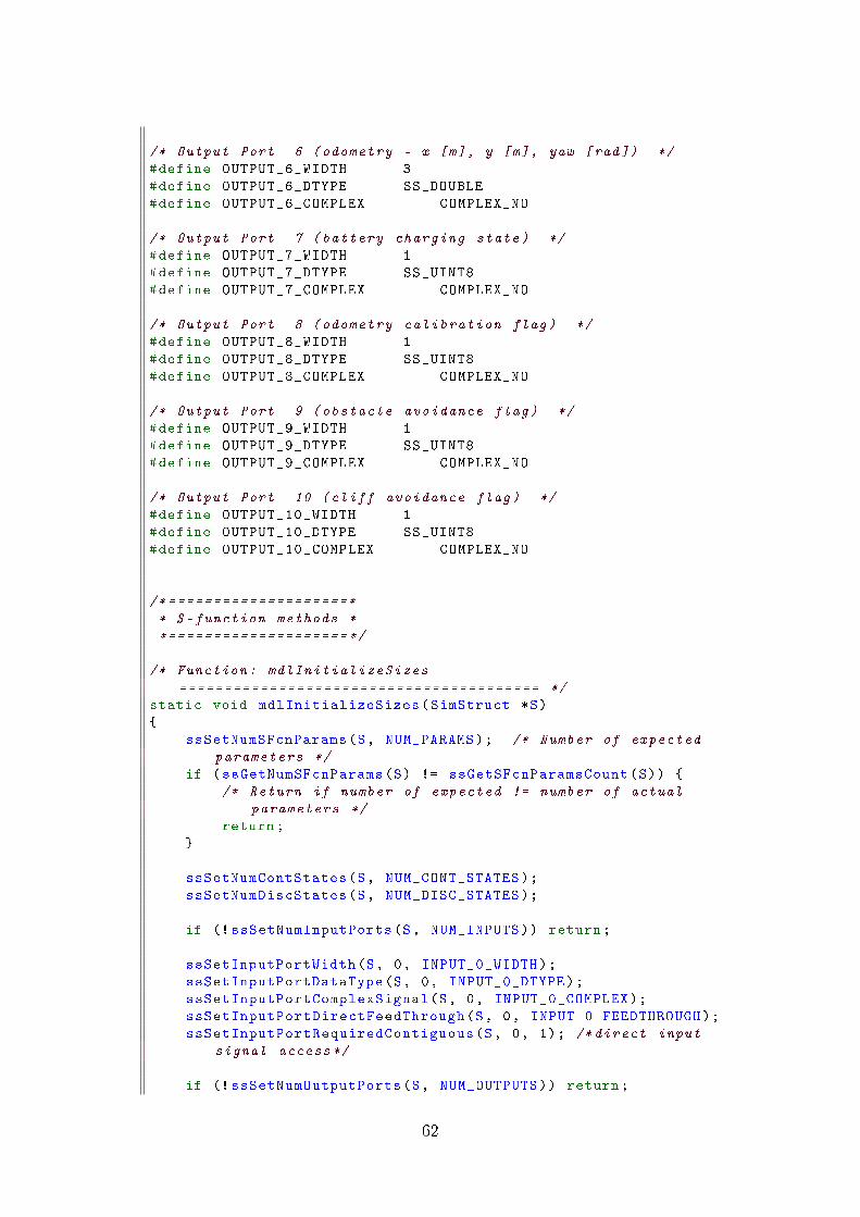
/* Output Port 6 (odometry - x [m], y [m], yaw [rad]) */


#define OUTPUT_6_DTYPE SS_DOUBLE


/* Output Port 7 (battery charging state) */




/* Output Port 8 (odometry calibration flag) */




/* Output Port 9 (obstacle avoidance flag) */




/* Output Port 10 (cliff avoidance flag) */




/* ====================*

* S-function methods *

*==================== */

/* Function: mdlInitializeSizes

======================================== */

static void mdlInitializeSizes(SimStruct *S)

{

ssSetNumSFcnParams(S, NUM_PARAMS); /* Number of expected

parameters */

if (ssGetNumSFcnParams(S) != ssGetSFcnParamsCount(S)) {

/* Return if number of expected != number of actual

parameters */

return;

}

ssSetNumContStates(S, NUM_CONT_STATES);

ssSetNumDiscStates(S, NUM_DISC_STATES);

if (! ssSetNumInputPorts(S, NUM_INPUTS)) return;

ssSetInputPortWidth(S, 0, INPUT_0_WIDTH);

ssSetInputPortDataType(S, 0, INPUT_0_DTYPE);

ssSetInputPortComplexSignal(S, 0, INPUT_0_COMPLEX);

ssSetInputPortDirectFeedThrough(S, 0, INPUT_0_FEEDTHROUGH);

ssSetInputPortRequiredContiguous(S, 0, 1); /* direct input

signal access */

if (! ssSetNumOutputPorts(S, NUM_OUTPUTS)) return;

62

ssSetOutputPortWidth(S, 0, OUTPUT_0_WIDTH);

ssSetOutputPortDataType(S, 0, OUTPUT_0_DTYPE);

ssSetOutputPortComplexSignal(S, 0, OUTPUT_0_COMPLEX);































ssSetNumSampleTimes(S, 1);

ssSetNumRWork(S, 0);

ssSetNumIWork(S, 0);

ssSetNumPWork(S, 0);

ssSetNumModes(S, 0);

ssSetNumNonsampledZCs(S, 0);

/* Specify the sim state compliance to be same as a built -in

block */

ssSetSimStateCompliance(S, USE_DEFAULT_SIM_STATE);

63

ssSetOptions(S, 0);

}

/* Function: mdlInitializeSampleTimes

================================== */

static void mdlInitializeSampleTimes(SimStruct *S)

{

ssSetSampleTime(S, 0, SAMPLE_TIME_0);

ssSetOffsetTime(S, 0, 0.0);

// notify need to access absolute time data

ssSetNeedAbsoluteTime(S, 1);

}

#undef MDL_INITIALIZE_CONDITIONS /* Change to #undef to remove

function */

#if defined(MDL_INITIALIZE_CONDITIONS)

/* Function: mdlInitializeConditions

================================= */

static void mdlInitializeConditions(SimStruct *S)

{

}

#endif /* MDL_INITIALIZE_CONDITIONS */

#define MDL_START /* Change to #undef to remove function */

#if defined(MDL_START)

/* Function: mdlStart

================================================ */

static void mdlStart(SimStruct *S)

{

}

#endif /* MDL_START */

/* Function: mdlOutputs

================================================ */

static void mdlOutputs(SimStruct *S, int_T tid)

{

}

#undef MDL_UPDATE /* Change to #undef to remove function */

#if defined(MDL_UPDATE)

/* Function: mdlUpdate

=============================================== */

static void mdlUpdate(SimStruct *S, int_T tid)

{

}

#endif /* MDL_UPDATE */

64

#undef MDL_DERIVATIVES /* Change to #undef to remove function

*/

#if defined(MDL_DERIVATIVES)

/* Function: mdlDerivatives

========================================== */

static void mdlDerivatives(SimStruct *S)

{

}

#endif /* MDL_DERIVATIVES */

/* Function: mdlTerminate

============================================== */

static void mdlTerminate(SimStruct *S){

}

/* =============================*

* Required S-function trailer *

*============================= */

#ifdef MATLAB_MEX_FILE /* Is this file being compiled as a

MEX -file? */

#include "simulink.c" /* MEX -file interface mechanism */

#else

#include "cg_sfun.h" /* Code generation registration

function */

#endif

65

A.2 sfun_wheelphone.tlc

%implements "sfun_wheelphone" "C"

%include "utillib.tlc"

%assign :: includeWheelphoneSupport = 1

%function BlockTypeSetup(block , system) void

%% %<LibAddToCommonIncludes("driver_wheelphone.h")>

%openfile buffer

extern void initWheelphone(void);

extern void getWheelphoneData(time_t , uint8_t *, uint8_t *,

uint8_t *,

uint8_t *, uint8_t *, int16_t *, double *,

uint8_t *,

uint8_t *, uint8_t *, uint8_t *);

extern void setWheelphoneSpeed(int32_t *, int32_t *);

extern void terminateWheelphone(void);

%closefile buffer

%<LibCacheFunctionPrototype(buffer)>

%<LibAddToModelSources("driver_wheelphone")>

%endfunction %% BlockTypeSetup

%function Start(block , system) Output

initWheelphone ();

%endfunction %% Start

%function Outputs(block , system) Output

/* %<Type > Block: %<Name > */

%assign pu0 = LibBlockInputSignalAddr (0, "", "", 0)

%assign pu1 = LibBlockInputSignalAddr (0, "", "", 1)

%assign py0 = LibBlockOutputSignalAddr (0, "", "", 0)











getWheelphoneData (%< LibGetTaskTimeFromTID(block)>,

%<py0 >, %<py1 >, %<py2 >, %<py3 >,

%<py4 >, %<py5 >, %<py6 >,

%<py7 >, %<py8 >, %<py9 >, %<py10 >);

66

setWheelphoneSpeed (%<pu0 >, %<pu1 >);

%endfunction %% Outputs

%function Terminate(block , system) Output

terminateWheelphone ();

%endfunction %% Terminate

67

A.3 driver_wheelphone.c

#include <jni.h>

#include <stdlib.h>

#include <math.h>

#define ENCODED_STATE_LEN 63

#define MAX_BATTERY_VALUE 152

#define SPEED_THR 3

#define NOT_CHARGING 0

#define CHARGING 1

#define CHARGED 2

#define LEFT_DIAM_COEFF 1.0

#define RIGHT_DIAM_COEFF 1.0

#define WHEEL_BASE 0.087

extern JavaVM *cachedJvm;

extern jobject cachedActivityObj;

extern jclass cachedMainActivityCls;

static jmethodID sgWheelphoneGetEncodedRobotStateID;

static jmethodID sgWheelphoneSetSpeedID;

static jmethodID sgWheelphoneSendCmdID;

static double leftDist = 0.0;

static double rightDist = 0.0;

static double leftDistPrev = 0.0;

static double rightDistPrev = 0.0;

static double timePrev = 0.0;

static double odometryX = 0.0;

static double odometryY = 0.0;

static double odometryTheta = 0.0;

void initWheelphone(void)

{

JNIEnv *pEnv;

(* cachedJvm)->AttachCurrentThread(cachedJvm , &pEnv , NULL);

sgWheelphoneGetEncodedRobotStateID = (*pEnv)->GetMethodID(

pEnv , cachedMainActivityCls ,

"getWheelphoneEncodedState","()[B");

sgWheelphoneSetSpeedID = (*pEnv)->GetMethodID(pEnv ,

cachedMainActivityCls ,

"setWheelphoneSpeed", "(II)V");

sgWheelphoneSendCmdID = (*pEnv)->GetMethodID(pEnv ,

cachedMainActivityCls ,

"sendWheelphoneCommands", "()V");

}

68

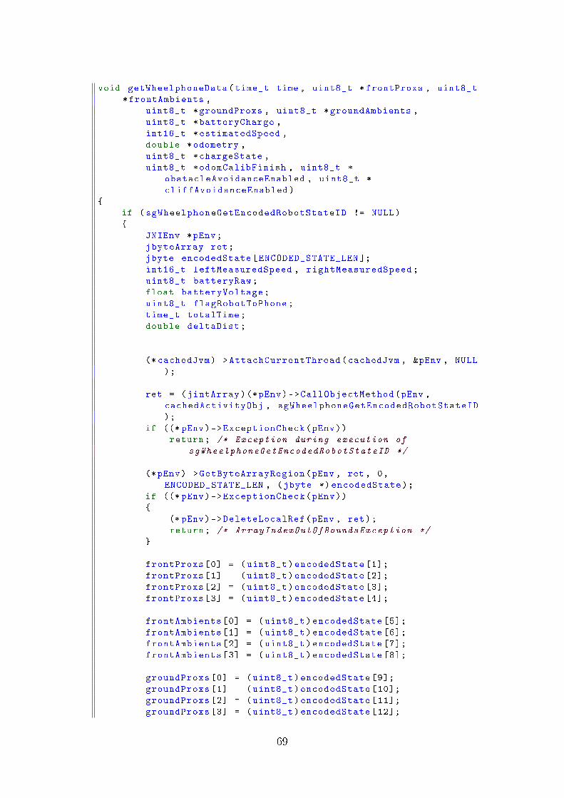
void getWheelphoneData(time_t time , uint8_t *frontProxs , uint8_t

*frontAmbients ,

uint8_t *groundProxs , uint8_t *groundAmbients ,

uint8_t *batteryCharge ,

int16_t *estimatedSpeed ,

double *odometry ,

uint8_t *chargeState ,

uint8_t *odomCalibFinish , uint8_t *

obstacleAvoidanceEnabled , uint8_t *

cliffAvoidanceEnabled)

{

if (sgWheelphoneGetEncodedRobotStateID != NULL)

{

JNIEnv *pEnv;

jbyteArray ret;

jbyte encodedState[ENCODED_STATE_LEN ];

int16_t leftMeasuredSpeed , rightMeasuredSpeed;

uint8_t batteryRaw;

float batteryVoltage;

uint8_t flagRobotToPhone;

time_t totalTime;

double deltaDist;

(* cachedJvm)->AttachCurrentThread(cachedJvm , &pEnv , NULL

);

ret = (jintArray)(*pEnv)->CallObjectMethod(pEnv ,

cachedActivityObj , sgWheelphoneGetEncodedRobotStateID

);

if ((* pEnv)->ExceptionCheck(pEnv))

return; /* Exception during execution of

sgWheelphoneGetEncodedRobotStateID */

(*pEnv)->GetByteArrayRegion(pEnv , ret , 0,

ENCODED_STATE_LEN , (jbyte *) encodedState);


{

(*pEnv)->DeleteLocalRef(pEnv , ret);

return; /* ArrayIndexOutOfBoundsException */

}

frontProxs [0] = (uint8_t)encodedState [1];




frontAmbients [0] = (uint8_t)encodedState [5];




groundProxs [0] = (uint8_t)encodedState [9];




69

groundAmbients [0] = (uint8_t)encodedState [13];




// battery level (from 0 to maxBatteryValue =152)

batteryRaw = (uint8_t)encodedState [17];

// battery voltage (from 3.5 to 4.2 volts)

// 915 is the ADC out at 4.2 volts

// 763 is the ADC out at 3.5 volts

// the "battery" variable actually contains the "

sampled value - 763"

batteryVoltage = 4.2*( float)(( batteryRaw + 763) /915.0);

// remaining battery charge (from 0% to 100%)

*batteryCharge = 100* batteryRaw/MAX_BATTERY_VALUE;

flagRobotToPhone = (uint8_t)encodedState [18];

// estimated speed (from back EMF) in [mm/s]

leftMeasuredSpeed = (uint8_t)encodedState [19] + 256*(

uint8_t)encodedState [20];

rightMeasuredSpeed = (uint8_t)encodedState [21] + 256*(

uint8_t)encodedState [22];

if (abs(leftMeasuredSpeed) < SPEED_THR) {

leftMeasuredSpeed = 0;

}

if (abs(rightMeasuredSpeed) < SPEED_THR) {

rightMeasuredSpeed = 0;

}

estimatedSpeed [0] = leftMeasuredSpeed;

estimatedSpeed [1] = rightMeasuredSpeed;

// estimated travelled distance [m]

leftDistPrev = leftDist;

rightDistPrev = rightDist;

totalTime = time - timePrev;

leftDist += (leftMeasuredSpeed /1000.0 * totalTime) *

LEFT_DIAM_COEFF;

rightDist += (rightMeasuredSpeed /1000.0 * totalTime) *

RIGHT_DIAM_COEFF;

deltaDist = (( rightDist - rightDistPrev) + (leftDist -

leftDistPrev)) / 2.0;

// odometry [m], [rad]

odometryX += cos(odometryTheta) * deltaDist;

odometryY += sin(odometryTheta) * deltaDist;

odometryTheta = (( rightDist - leftDist) / WHEEL_BASE) /

1000.0;

odometry [0] = odometryX;

odometry [1] = odometryY;

70

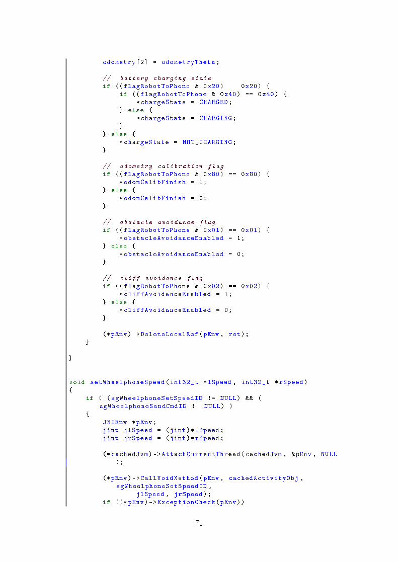
odometry [2] = odometryTheta;

// battery charging state

if (( flagRobotToPhone & 0x20) == 0x20) {


*chargeState = CHARGED;

} else {

*chargeState = CHARGING;

}

} else {

*chargeState = NOT_CHARGING;

}

// odometry calibration flag


*odomCalibFinish = 1;

} else {

*odomCalibFinish = 0;

}

// obstacle avoidance flag


*obstacleAvoidanceEnabled = 1;

} else {

*obstacleAvoidanceEnabled = 0;

}

// cliff avoidance flag


*cliffAvoidanceEnabled = 1;

} else {

*cliffAvoidanceEnabled = 0;

}

(*pEnv)->DeleteLocalRef(pEnv , ret);

}

}

void setWheelphoneSpeed(int32_t *lSpeed , int32_t *rSpeed)

{

if ( (sgWheelphoneSetSpeedID != NULL) && (

sgWheelphoneSendCmdID != NULL) )

{

JNIEnv *pEnv;

jint jlSpeed = (jint)*lSpeed;

jint jrSpeed = (jint)*rSpeed;

(* cachedJvm)->AttachCurrentThread(cachedJvm , &pEnv , NULL

);

(*pEnv)->CallVoidMethod(pEnv , cachedActivityObj ,

sgWheelphoneSetSpeedID ,

jlSpeed , jrSpeed);


71


sgWheelphoneSetSpeedID */

(*pEnv)->CallVoidMethod(pEnv , cachedActivityObj ,

sgWheelphoneSendCmdID);



sgWheelphoneSendCmdID */

}

}

void terminateWheelphone(void){

}

72

A.4 wheelphonelib.tlc

%function FcnGenWheelphoneLib () void

%assign tgtData = FEVAL("get_param", CompiledModel.Name ,

"TargetExtensionData")

%assign packageName = "%<tgtData.packagename >.%<

CompiledModel.Name >"

%openfile wheelphoneLibFile = "WheelphoneRobot.java"

%selectfile wheelphoneLibFile

package %<packageName >;

import android.content.Context;

import android.content.Intent;

import android.os.Handler;

import android.os.Message;

public class WheelphoneRobot {

// USB communication

private final static int packetLengthRecv = 63;

private final static int packetLengthSend = 63;

private final static int USBAccessoryWhat = 0;

private static final int APP_CONNECT = (int) 0xFE;

private static final int APP_DISCONNECT = (int) 0xFF;

private static final int UPDATE_STATE = 4;

private boolean deviceAttached = false;

private boolean isConnected = false;

private int firmwareVersion = 0;

private USBAccessoryManager accessoryManager;

// Packet received from PIC with encoded robot state

private byte[] encodedRobotState = new byte[packetLengthRecv

];

// Robot control (phone => robot)

private int lSpeed = 0, rSpeed = 0;

private static final int MIN_SPEED_RAW = -127;

private static final int MAX_SPEED_RAW = 127;

private static final int MIN_SPEED_REAL = -350;

private static final int MAX_SPEED_REAL = 350;

private static final double MM_S_TO_BYTE = 2.8;

private byte flagPhoneToRobot = 1;

// bit 0 => controller On/Off

// bit 1 => soft acceleration On/Off

// bit 2 => obstacle avoidance On/Off

// bit 3 => cliff avoidance On/Off

// others bits not used

private Context context;

private Intent activityIntent;

73

/*

* Interface that should be implemented by classes that

would like to

* be notified by when the WheelphoneRobot state is updated.

*/

public interface WheelphoneRobotListener {

void onWheelphoneUpdate ();

}

private WheelphoneRobotListener mEventListener;

// Handler for receiving messages from the USB Manager

thread

private Handler handler = new Handler () {

public void handleMessage(Message msg) {

byte[] commandPacket1 = new byte [2];

byte[] commandPacket2 = new byte[packetLengthSend ];

switch (msg.what) {

case USBAccessoryWhat:

switch ((( USBAccessoryManagerMessage) msg.

obj).type) {

case CONNECTED:

break;

case DISCONNECTED:

isConnected = false;

// Notify listener of a disconnection

if(mEventListener !=null) {

mEventListener.

onWheelphoneUpdate ();

}

break;

case READY:

String version = ((

USBAccessoryManagerMessage) msg.

obj).accessory.getVersion ();

firmwareVersion = getFirmwareVersion

(version);

switch (firmwareVersion) {

case 1:

deviceAttached = true;

break;

74

case 3:

// send information PIC

commandPacket1 [0] = (byte)

APP\_CONNECT;

commandPacket1 [1] = 0;

accessoryManager.write(

commandPacket1);

deviceAttached = true;

// Wheelphone state


UPDATE\_STATE;


0;


0;

commandPacket2 [3] =

flagPhoneToRobot;

accessoryManager.write(

commandPacket2);

break;

default:

break;

}

isConnected = true;

break;

case READ:

if (accessoryManager.isConnected ()

== false) {

return;

}

while (true) {

if (accessoryManager.available ()

< packetLengthRecv) {

break;

}

accessoryManager.read(

encodedRobotState);

switch(encodedRobotState [0]) {

case UPDATE\_STATE:

// Notify listener of an

update

if(mEventListener !=null)

{

mEventListener.

onWheelphoneUpdate

();

}

75

break;

}

}

break;

case ERROR:

break;

default:

break;

}

}

}

};

/**

* brief Class constructor

* param a pass the main activity instance (this)

* return WheelphoneRobot instance

*/

public WheelphoneRobot(Context c, Intent i) {

context = c;

activityIntent = i;

mEventListener = null;

}

public void createUSBCommunication () {

accessoryManager = new USBAccessoryManager(handler ,

USBAccessoryWhat);

}

/**

* brief To be inserted into the "onResume" function of the

main activity class.

* return none

*/

public void openUSBCommunication () {

accessoryManager.enable(context , activityIntent);

}

/**

* brief To be inserted into the "onPause" function of the

main activity class.

* return none

*/

public void closeUSBCommunication () {

76

accessoryManager.disable(context);

switch (firmwareVersion) {

case 2:

case 3:

byte[] commandPacket = new byte [2];

commandPacket [0] = (byte) APP\_DISCONNECT;

commandPacket [1] = 0;

accessoryManager.write(commandPacket);

break;

}

try {

while (accessoryManager.isClosed () == false) {

Thread.sleep (2000);

}

} catch (InterruptedException e) {

e.printStackTrace ();

}

isConnected = false;

}

/**

* brief Set listener to be notified by when the

WheelphoneRobot state is updated. .

* return none

*/

public void setWheelphoneRobotListener(

WheelphoneRobotListener eventListener) {

mEventListener = eventListener;

}

/**

* brief Remove listener to be notified by when the

WheelphoneRobot state is updated. .

* return none

*/

public void removeWheelphoneRobotListener () {

mEventListener = null;

}

/**

* brief Send the next packet to the robot containing the

last left and right speeds and flag data.

* Use the speed references set with the setSpeed methods.

* return none

*/

public void sendCommandsToRobot () {

if (accessoryManager.isConnected () == false) {

return;

}

byte[] commandPacket = new byte[packetLengthSend ];

77

commandPacket [0] = (byte) UPDATE\_STATE;

commandPacket [1] = (byte) lSpeed; // left

speed ref

commandPacket [2] = (byte) rSpeed; // right

speed ref

commandPacket [3] = flagPhoneToRobot; // (control

enable)


}

/**

* brief Turn Wheelphone motors off.

* return none

*/

public void turnMotorsOff () {

if (accessoryManager.isConnected () == false) {

return;

}

byte[] commandPacket = new byte[packetLengthSend ];

commandPacket [0] = (byte) UPDATE\_STATE;

commandPacket [1] = 0; // left

speed ref

commandPacket [2] = 0; // right

speed ref

commandPacket [3] = flagPhoneToRobot; // (control

enable)


}

/**

* brief Retrieve firmware version from USB version

* param string with USB version

* return firmware version installed on Wheelphone PIC24F

*/

private int getFirmwareVersion(String version) {

String major = "0";

int positionOfDot;

positionOfDot = version.indexOf('.');

if (positionOfDot != -1) {

major = version.substring (0, positionOfDot);

}

return new Integer(major).intValue ();

}

/**

* brief Return version of the firmware running on the robot

. This is useful to know whether an update is available

or not.

* return firmware version

*/

public int getFirmwareVersion () {

78

return firmwareVersion;

}

/**

* brief Return the encoded robot state (i.e. packet

received from onboard PIC)

* return encoded robot state

*/

public byte[] getEncodedRobotState () {

return encodedRobotState;

}

/**

* brief Indicate whether the robot is connected (and

exchanging packets) with the phone or not.

* return true (if robot connected), false otherwise

*/

public boolean isRobotConnected () {

return isConnected;

}

/**

* brief Set the new left and right speeds for the robot.

The new data

* will be actually sent to the robot when "

sendCommandsToRobot" is

* called the next time within the timer communication task

(50 ms cadence).

* This means that the robot speed will be updated after

* at most 50 ms (if the task isn't delayed by the system).

* param l left speed given in mm/s

* param r right speed given in mm/s

* return none

*/

public void setSpeed(int l, int r) { // speed given

in mm/s

if(l < MIN\_SPEED\_REAL) {

l = MIN\_SPEED\_REAL;

}

if(l > MAX\_SPEED\_REAL) {

l = MAX\_SPEED\_REAL;

}

if(r < MIN\_SPEED\_REAL) {

r = MIN\_SPEED\_REAL;

}

if(r > MAX\_SPEED\_REAL) {

r = MAX\_SPEED\_REAL;

}

lSpeed = (int) (l/MM\_S\_TO\_BYTE);

rSpeed = (int) (r/MM\_S\_TO\_BYTE);

}

79

/**

* brief Set the new left and right speeds for the robot.

For more details refer to "setSpeed ".

* param l left speed (range is from -127 to 127)

* param r right speed (range is from -127 to 127)

* return none

*/

public void setRawSpeed(int l, int r) {

if(l < MIN\_SPEED\_RAW) {

l = MIN\_SPEED\_RAW;

}

if(l > MAX\_SPEED\_RAW) {

l = MAX\_SPEED\_RAW;

}

if(r < MIN\_SPEED\_RAW) {

r = MIN\_SPEED\_RAW;

}

if(r > MAX\_SPEED\_RAW) {

r = MAX\_SPEED\_RAW;

}

lSpeed = l;

rSpeed = r;

}

%closefile wheelphoneLibFile

%endfunction

80

References

[1] S. Bhattacharya, R. Ghrist, and V. Kumar. Multi-robot Coverage and Ex-ploration on Riemannian Manifolds with Boundary. International Journal ofRobotics Research, 33(1):113�137, January 2014.

[2] F. Bullo, R. Carli, and P. Frasca. Gossip Coverage Control for Robotic Net-works: Dynamical Systems on the Space of Partitions. SIAM Journal on Con-trol and Optimization, 50(1):419�447, 2012.

[3] J. Choi, S. Oh, and R. Horowitz. Distributed learning and cooperative controlfor multi-agent systems. Automatica, 45(12):2802�2814, 2009.

[4] J. Cortés and F. Bullo. Coordination and geometric optimization via distributeddynamical systems. SIAM Journal on Control and Optimization, 44(5):1543�1574, 2005.

[5] J.Cortes,S.Martinez,T.Karatas,andF.Bullo. Coverage control for mobile sensingnetworks. Automatica, 20(2):243�255, 2004.

[6] J. Cortes, S. Martinez, T. Karatas, and F. Bullo. Coverage control for mobilesensing networks. Robotics and Automation, IEEE Transactions on, 20(2):243�255, April 2004.

[7] P. Davison, M. Schwemmer, and N.E. Leonard. Distributed nonuniform cover-age with limited scalar measurements. In Communication, Control, and Com-puting (Allerton), 2012 50th Annual Allerton Conference on, pages 1455�1460.IEEE, 2012.

[8] A.A. de Menezes Pereira, H.K. Heidarsson, C. Oberg, D.A. Caron, B.H. Jones,and G.S. Sukhatme. A CommunicationFrameworkforCost-e�ectiveOperationofAUVs in Coastal Regions. In The 7th International Conference on Field andService Robots, Cambridge, Massachusetts, 2009.

[9] Q. Du, V. Faber, and M. Gunzburger. Centroidal Voronoi tessellations: appli-cations and algorithms. SIAM review, 41(4):637�676, 1999.

[10] J. W. Durham, R. Carli, P. Frasca, and F. Bullo. Discrete Partitioning andCoverage Control for Gossiping Robots. Robotics, IEEE Transactions on,28(2):364� 378, 2012.

[11] S.G. Lee, Y. Diaz-Mercado, and M. Egerstedt. Multirobot Control Using Time-Varying Density Functions. Robotics, IEEE Transactions on, 31(2):489�493,April 2015.

[12] N.E. Leonard and A. Olshevsky. Nonuniform coverage control on the line. InDecision and Control and European Control Conference (CDC-ECC), 2011 50thIEEE Conference on, pages 753�758. IEEE, 2011.

81

[13] N.E. Leonard, D.A. Paley, F. Lekien, R. Sepulchre, D.M. Fratantoni, and R.E.Davis. Collective Motion, Sensor Networks, and Ocean Sampling. Proceedingsof the IEEE, 95(1):48�74, Jan 2007.

[14] S. Lloyd. Least squares quantization in PCM. Information Theory, IEEE Trans-actions on, 28(2):129�137, Mar 1982.

[15] K.M. Lynch, I.B. Schwartz, P. Yang, and R.A. Freeman. Decentralized envi-ronmental modeling by mobile sensor networks. Robotics, IEEE Transactionson, 24(3):710�724, 2008.

[16] R. Patel, P. Frasca, J. W. Durham, R. Carli, and F. Bullo. Dy-namic Partitioning and Coverage Control with Asynchronous One-To-Base-StationCommunication. Control of Network Systems, IEEE Transaction on,2015. To appear.

[17] M. Schwager, D. Rus, and J-J. Slotine. Decentralized, adaptive coverage con-trol for networked robots. The International Journal of Robotics Research,28(3):357�375, 2009.

[18] M.Schwager,M.P.Vitus,S.Powers,D.Rus,andC.J. Tomlin. Robust adaptive cov-erage control for robotic sensor networks. IEEE Transactions on Control ofNetwork Systems, 2014.

[19] R.C. Shah, S. Roy, S. Jain, and W. Brunette. Data MULEs: modeling a three-tier architecture for sparse sensornetworks. In Sensor Network Protocols andApplications, 2003. Proceedings of the First IEEE. 2003 IEEE InternationalWorkshop on, pages 30�41, May 2003.

[20] M. Todescato, A. Carron, R. Carli, G. Pillonetto, and L. Schenato. Video ofSB algorithm available athttp://automatica.dei.unipd.it/people/todescato/publications.html.

[21] Y. Xu, J. Choi, S. Dass, and T. Maiti. E�cient Bayesian spatial predictionwith mobile sensor networks using Gaussian Markov random �elds, Automatica,49(12):3520�3530, 2013.

[22] M. Todescato, A. Carron, R. Carli,G. Pillonetto, L. Schenato Multi-RobotsGaussian Estimation and Coverage Control: from Client-Server to Peer-to-PeerArchitectures, Automatica, 2016

[23] Y. Xu, J. Choi, andS. Oh. Mobile sensor network navigation using Gaussian pro-cesses with truncated observations. IEEE Transactions on Robotics, 27(6):1118�1131, 2011.

[24] http://www.btsbioengineering.com/it/

[25] K.S.Arun,T.S.Huang,S.D.Blostein, Least-Square Fitting of two 3D Point Set

82

universitÁ degli studi di padoav corso di...

Documents