universitÀ degli studi di cagliari facoltÀ …€ degli studi di cagliari facoltÀ di ingegneria...
TRANSCRIPT

UNIVERSITÀ DEGLI STUDI DI CAGLIARI
FACOLTÀ DI INGEGNERIA
CORSO DI LAUREA SPECIALISTICA IN INGEGNERIA MECCANICA
ANNO ACCADEMICO 2006-2007
WIND ENERGY RESOURCE EVALUATION IN A SITE OF CENTRAL
ITALY BY CFD SIMULATIONS
Relatore: Tesi di laurea di:
Dott. Ing. Francesco Cambuli Daniele Fallo
Correlatore:
Dott. Ing. Giorgio Crasto
D.I.Me.Ca. Dipartimento di Ingegneria Meccanica – Cagliari

Se un uomo sogna da solo, il sogno rimane solo un sogno,
ma se molti uomini sognano la stessa cosa, il sogno diventa realtà.
Dom Helder Camara (1909-1999)

I
Index Index page I
Acknowledgments VI
Introduction 1
CHAPTER 1. Atmospheric Boundary Layer 4
1.1 The Atmospheric Boundary Layer (ABL) 4
1.2 Description of the ABL 4
1.3 Mathematical formulation of the ABL 5
1.4 Navier-Stokes and RANS equations 6
1.5 The WindSim numerical code 8
1.5.1 Terrain 8
1.5.2 Windfield 9
Boundary conditions 9
Turbulence model 9
Solver 10
1.5.3 Objects 10
Turbines 10
Climatologies 10
Transferred climatologies 10
1.5.4 Results 12
1.5.5 Wind Resources 12
1.5.6 Energy 12
II
1.6 κ−ε turbulence model page 12
CHAPTER 2: Simulations over flat terrains 16
2.1 Introduction 16
2.2 Geometrical model and inlet BC 17
2.3 Vertical discretization sensitivity 18
2.4 Height distribution factor sensitivity 20
2.5 Influence of the top boundary condition 22
2.6 Remarks 25
CHAPTER 3: Simulations over 2D hilly terrains 26
3.1 Introduction 26
3.1.1 Similitude between a 3D “cos2” and “flatted” hill 26
3.2 Speed-up effect 30
3.3 Sensitivity to the first cell height 33
3.4 Sensitivity to the horizontal discretization 35
3.5 Investigation of a flow over a 2D roughly hilly terrain 37
3.5.1 Description of the test case 37
3.5.2 Numerical method 39
3.5.3 Case S3H4 40
3.5.4 Case S5H4 41
3.5.5 Results 43
Case S3H4 43
Case S5H4 45
3.6 Remarks 48
III
CHAPTER 4: Characteristics of the site page 49
4.1 Introduction 49
4.2 Digital terrain model (DTM) 50
4.2.1 Orographic characteristics of the site 50
4.2.2 Roughness characteristics 52
4.3 Wind data 55
4.3.1 Mast 5424-30 m - period April-May 2007 59
4.3.2 Mast 5424-15 m - period April-May 2007 60
4.3.3 Mast 5424-30 m - period November-December 2006 61
4.3.4 Mast 5424-15 m - period November-December 2006 62
4.3.5 Mast 5428-50 m - period April-May 2007 63
4.3.6 Mast 5428-40 m- period April-May 2007 64
4.3.7 Mast 5428-30 m- period April-May 2007 65
4.3.8 Mast 5428-50 m - period November-December 2006 66
4.3.9 Mast 5428-40 m- period November-December 2006 67
4.3.10 Mast 5428-30 m- period November-December 2006 68
4.4 Mean speed per sector tables 69
4.4.1 Mast 5424 69
4.4.2 Mast 5428 70
4.5 Power density per sector tables 71
4.5.1 Mast 5424 71
4.5.2 Mast 5428 72
4.6 Remarks 7

IV
CHAPTER 5: Test of the Free Stream Velocity (FSV) page 74
5.1 Introduction 74
5.2 Mesoscale model 74
Geometrical model 75
Numerical model 75
5.3 Microscale model – evidence of recirculation 77
Geometrical model 78
Numerical model 78
5.4 Microscale model – final speed-up maps 81
Geometrical model 82
Numerical model 83
5.5 Remarks 84
CHAPTER 6: Analysis of the wind field over the site 90
6.1 Introduction 90
6.2 Geometrical model 90
6.3 Numerical model 91
6.4 Simulations 92
6.5 Vertical profiles of velocity 94
Tower 5424 (Cliff) 94
Tower 5428 (Plateau) 97
6.6 Turbulence Intensity vertical profiles 101
Tower 5424 (Cliff) 102
Tower 5428 (Plateau) 105
6.7 Cross-checking of wind data 108
Sector Interpolation 108
V
6.7.1 Mean wind velocity page 109
6.7.2 Speed-up 113
Period April-May 2007 113
Period November-December 2006 115
6.8 Remarks 118
CHAPTER 7: Proposal for a plant layout 119
7.1 Introduction 119
7.2 Dataset April-May 5428-50 m 119
7.3 Wind resources 120
7.4 Annual energy production AEP 122
7.5 Remarks 125
Conclusions 126
Bibliography 128

VI
Acknowledgments La redazione di questa mia tesi di laurea è il risultato di uno stage svolto presso la compagnia WindSim AS di Tonsberg, in Norvegia. A tal proposito devo ringraziare il Dott. Arne Reidar Gravdahl e la Dott.sa Tine Volstad e, con loro, tutto il team WindSim con i quali ho avuto il piacere di collaborare in questi ultimi mesi. Arne e Tine si sono rivelate due persone speciali e hanno fatto si che la mia permanenza in Norvegia fosse confortevole anche al di fuori delle ore lavorative, facendomi assaporare i piaceri della vera tradizione norvegese e trattandomi come una persona di famiglia. Un particolare ringraziamento va al Dott. Francesco Bonomo della sezione dell’ENEL Produzione di Catania, per aver fornito i dati digitali del terreno e i dati anemometrici del sito analizzato, senza i quali tutto questo lavoro non sarebbe mai potuto essere realizzato. Un ringraziamento speciale va inoltre al mio relatore, il gentilissimo e sempre disponibile Dott. Ing. Francesco Cambuli del D.I.Me.Ca., il quale mi ha introdotto alla conoscenza della fluidodinamica numerica e mi ha incoraggiato (ed in qualche modo convinto) ad affrontare questa bellissima esperienza all’estero, fornendomi nonostante la distanza, un validissimo aiuto on-line durante tutti questi mesi. E poi viene lui, il monumentale Dott. Ing. Giorgio Crasto, lo stesso del team WindSim con il quale ho condiviso gli spazi e i gustosi pranzi nel WindSim Office, e lo stesso che mi fece da tutor durante la redazione della tesi di laurea triennale. Lo stesso Giorgio mi ha aiutato ad affrontare gli innumerevoli problemi della fluidodinamica numerica e che ha condiviso con me la maggior parte del nostro tempo libero durante i mesi di permanenza in Norvegia, rivelandosi oltre che un bravo tutor, un gran cuoco ed anche un buon amico. Questi anni trascorsi a Cagliari non sarebbero stati lo stesso se non fosse stato per il supporto dei miei colleghi del corso di Ingegneria Meccanica, ai quali va un mio caloroso ringraziamento per aver condiviso gioie e dolori di un corso di studi bello e faticoso. Infine devo ringraziare la mia famiglia, Angelo, Cecchina ed Irene, che mi sono sempre stati vicini, hanno sempre creduto in me e si sono adoperati per facilitarmi nello studio. L’ultimo ringraziamento ho voluto conservarlo per Silvia, per la “solita” pazienza e comprensione dimostratami (duramente testate già ai tempi della laurea triennale !) e che anche nei momenti di maggior stress ha saputo regalarmi un sorriso.

VII
This thesis is the result of a practice period at the WindSim AS company of Tonsberg, Norway. Regarding that, I have to thank Doc. Arne Reidar Gravdahl and Doct. Tine Volstad and, with them, the whole WindSim Team in which I took part during these last months. Arne & Tine were two persons special and kind toward me, even after work, and they let me to taste the real Norwegian tradition and treated me as a person of their family. A special thank to Doc. Francesco Bonomo of the ENEL Produzione, Section of Catania, Italy for providing digital terrain maps an wind data. A special thank also to my University tutor, Doc. Eng. Francesco Cambuli of the DIMECA of Cagliari, for introducing me to the study of the computational fluid dynamics and for encouraging me to start a new experience abroad. He has been very kind in giving me on-line support during these months spent in Norway. A very special thank to Doc. Eng. Giorgio Crasto, part of the WindSim Team, which has been my colleague at the WindSim main Office and was always kind in helping me to solve the problems of the CFD. Thanks a lot to my University colleagues of the Course in Mechanical Engineering, for their support and team spirit, and to my family, Angelo, Cecchina and Irene, which have been always believing in my potential and facilitated the years spent at the University. The last thank is for Silvia, which has been always patient and comprehensive with me and always able to offer me a smile.

1
Introduction
The present work aims to improve part of the technologies nowadays used in the
production of electrical energy by renewable sources, particularly energy coming
from the wind. This tendency is supported by the deeper aim, especially in the
European Union, to be more and more independent from extra-communitarian
Countries in fossil energy sources import and to be even more awake in protecting
the environment from pollutant.
The actual world situation demonstrates how much, from an economic point of
view, to dispose of primary energy sources is important. In fact, the first
consequence of this subordination condition is the high cost of the energy, which is
going to grow more and more due to the limited fossil energy sources, causing a risk
of degeneration in the war to own the energy resources.
It is evident, nowadays, that a change in the direction of the diversification of the
energy resources is needed, giving importance to the renewable energies.
Wind Energy is an ancient Energy source, used in its first applications already during
Persian Emperor, more than 2000 years ago. Its use has been widely diffused in
various Countries of the world and, in the present days, the wind energy
technologies arrived to a mature level.
The first step in projecting a wind farm is the prediction of the wind resources and,
for this scope, various techniques are used. Linear models, like Was’P (Wind Atlas
Analysis and Application Program), are widely used where the terrain is
characterized by simple orography. Linear models use linear equations to describe
the behavior of the flow over a territory, but can encounter some problems in
evaluating wind characteristics when the region becomes complex, where hills and
steep mountains are present.
In these cases the use of other methods, like Computational Fluid Dynamics (CFD) is
preferred [15]. CFD solves, by using numerical methods, the Reynolds Averaged
Navier-Stokes (RANS) equations to predicts the flow over the site. In this thesis this
calculation is done by the software WindSim.

2
WindSim is a software developed by the company WindSim AS of Tonsberg, Norway,
which bears on the CFD software PHOENICS, to solve the RANS equations using the
finite volume method and has a series of packages allowing wind energy analysis.
The present Master Thesis is the final work of a training period of 6 months spent by
the author at the main office of WindSim company, during the last year of his
studying in Mechanical Engineering.
The work encompasses a starting validation phase of the CFD numerical code,
focused to obtain the correct parameters and boundary condition able to describe
with a fair accuracy the behavior of the Atmospheric Boundary Layer (ABL).
Various problematic about wind farms projects have been afforded. A collaboration
with the company Enel Produzione of Catania, Italy, has been set up and carried on,
in order to perform the study of the wind energy resources in a site of central Italy,
about which the company was interested in. Particularly, two short-period sets of
available experimental wind data have been analysed by a procedure addressed to
validate the CFD calculation over the complex orography of the site. Wind resources
maps of the site were obtained and the project of a wind farm siting was proposed.
This Master Thesis is subdivided in 7 chapters: the first one describes the general
characteristics of the ABL and its mathematical formulation. Moreover, a brief
description of the WindSim numerical code and its graphical interface is presented.
In chapter 2 and 3 the correct boundary conditions, grid and solver settings to be
applied to the model in order to describe the ABL are analyzed, by means of
comparison of the CFD predictions with results found in literature. Next chapter
describes the wind characteristics of a site located in central Italy, together with the
analysis of the experimental wind data available. Particular attention is done in
finding the dominant sectors of the wind rose. Chapters 5 and 6 are related to the
simulation of the flow field over the site. The “nesting technique” have been used in
chapter 5 to determine the free stream velocity boundary conditions needed to
describe the geostrophic wind over the site. Chapter 6 describes the geometrical
and numerical model used to simulate the wind field over the whole site area. The
procedure to match numerical results and of the available experimental data is

3
explained and performed. Finally, chapter 7 presents the wind resources map of the
site and a proposal for a wind farm layout.

4
CHAPTER 1. Atmospheric Boundary Layer.
1.1 The Atmospheric Boundary Layer The Atmospheric Boundary Layer (ABL) is the lowest part of the atmosphere and its
behavior is directly influenced by the interaction with a planetary surface, according
to Stull, R. B. (1988) [12].
It’s known that the ABL responds to surface forcing in a timescale of one hour or
less, while the typical space scale is few kilometers. In this layer physical quantities
such as flow velocity, temperature, moisture, etc. display relatively rapid
fluctuations.
Above the ABL there is the “free atmosphere”, where the wind is considered
geostrophic (parallel to isobars), while inside the ABL the wind is affected by surface
effects and turns across the isobars.
1.2 Description of the ABL The ABL is a part of the troposphere which is the lowest portion of Earth's
atmosphere. It contains approximately 75% of the atmosphere's mass and almost all
of its water vapor and aerosols.
The average depth of the troposphere is about 11 km in the middle latitudes. It is
deeper in the tropical regions (up to 20 km) and shallower near the poles (about 7
km).
As already said, the lowest part of the troposphere is the ABL and this layer is about
2 km deep, depending on the landform and time of day.
In a neutral ABL, where heat transfer is not taken into account, several sub-layers
can be identified.
The canopy layer is the first sub-layer near the terrain, where obstacles are present;
above it, the surface layer can be found, in which Coriolis effects are negligible;
finally there is the so called Ekman layer, where Coriolis effects are dominant.

5
1.3 Mathematical formulation of the ABL The Atmospheric Boundary Layer can be described through very simple
mathematical equations using the so called surface-layer similarity, also known as
Monin-Obukhov similarity.
According to this, the speed vertical profile of the wind can be described as a
function of the height by the logarithmic profile,
1.1) ( ) = ∙
where,
is the friction velocity [m/s]
is the Von Karman constant [ ]
is the roughness height [m]
The friction velocity is calculated by the equation
1.2) =
where,
τ is the shear stress at the wall boundary [N/m2]
is the air density [kg/m3]
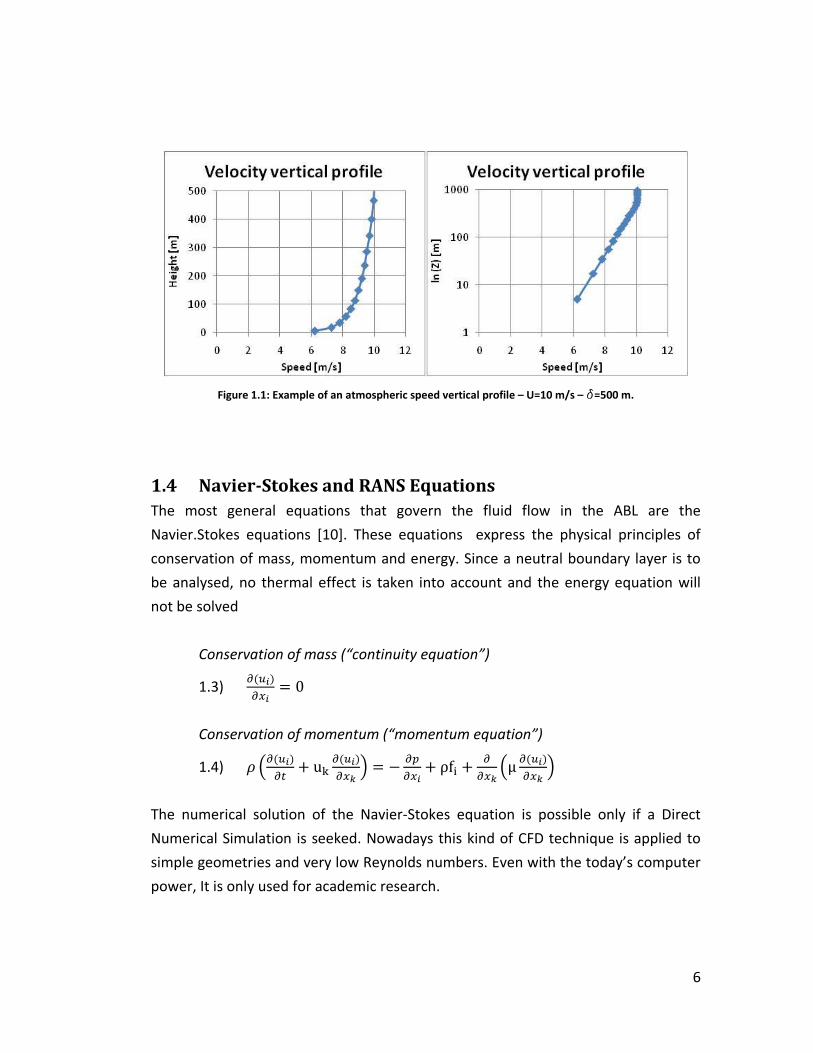
An example of a velocity vertical profile, is shown in figure 1.1
6
Figure 1.1: Example of an atmospheric speed vertical profile – U=10 m/s – d=500 m.
1.4 Navier-Stokes and RANS Equations The most general equations that govern the fluid flow in the ABL are the
Navier.Stokes equations [10]. These equations express the physical principles of
conservation of mass, momentum and energy. Since a neutral boundary layer is to
be analysed, no thermal effect is taken into account and the energy equation will
not be solved
Conservation of mass (“continuity equation”)
1.3) ( ) = 0
Conservation of momentum (“momentum equation”)
1.4) ( ) + u ( ) = − + ρf + μ ( )
The numerical solution of the Navier-Stokes equation is possible only if a Direct
Numerical Simulation is seeked. Nowadays this kind of CFD technique is applied to
simple geometries and very low Reynolds numbers. Even with the today’s computer
power, It is only used for academic research.

7
Turbulence is typical of industrial and atmospheric flows. Two different ways can be
pursued with the goal of solving the turbulence problem for real flows using CFD.
The first method numerically solves the Large Eddy Simulation (LES) equation, while
the second uses the Reynolds Averaged Navier-Stokes equation.
LES equation are deduced from Navier-Stokes Equation with a spatial averaging
process. In this way only the large scale vortices are numerically solved, while the
small scale turbulence Is “modelled”. LES simulation were introduced [7] to solve the
mesoscale atmospheric flow and today are also used for industrial flow, even
though a very high computer power in terms of CPU and RAM is required.
The most used way to solve real flows with a relatively low computer cost is solving
the RANS equations. These equation, displayed in equations 1.5 and 1.6, are again
deduced from the N-S equation, but using a time averaging procedure instead. In
this way all the turbulence is modeled and only the time averaged variables are
found with the simulations.
Continuity equation
1.5) = 0
Momentum equation
1.6) ∙ = ∙ − − ∙ +
In the RANS equations, terms that take account for turbulence appear. A
relationship between these terms and the time averaged variables is needed to
close and solve the system of RANS equations. Different turbulence models are used
to close the system of RANS equations, mainly based on the Boussinesque
hypothesis [6]. An example is shown by equation
1.7) − = ∙ + − + ∙ ∙

8
1.5 The WindSim numerical code WindSim is a CFD code used for evaluate the wind resources in a site by solving the
RANS equations. It is produced by the company WindSim AS, Norway.
WindSim uses a core constituted by the solver Phoenics (developed by Cham, UK),
which solves the RANS equations with the finite volume method [11].
WindSim contains a group of accessory software which help in the solution of
atmospheric flows.
WindSim is constituted by 6 modules, which have to be run in sequence: the user is
not able to run the further module if the previous one hasn’t completed its work.
The modules are listed below.
1 Terrain 2 Windfield 3 Objects 4 Results 5 Wind Resources 6 Energy
A brief description of each module is now reported, in order to analyze the main
input parameters and output results.
1.5.1 TERRAIN In this module all informations regarding orography and roughness of the site of
interest are inserted, through the file ***.gws . The ***.gws file is a characteristic
WindSim format that can be created by the automatic conversion module, also
present in WindSim. In this way, WAsP files and ***.xyz files can be used to set
terrain informations.
The Terrain module also allows the user to define the parameters of the geometrical
model, setting the grid discretization and the number of cells. Moreover, a lot of
other important settings needed for CFD simulations can be defined.

9
1.5.2 WINDFIELD The Windfield module calculate the wind characteristics of the site of interest. To do
this the Reynolds Averaged Navier-Stokes equations are solved, using the finite
volume numerical method with the CFD solver “PHOENICS”
In this module the boundary conditions, the turbulence model and the solver
settings can be defined by the user.
Boundary conditions
The wind velocity vertical profile must be set by defining the height of the ABL, the
free stream velocity of the geostrophic wind and the wind direction. The ABL is
described through the log law (refer to chapter 1), while the wind direction can be
set by subdividing the wind rose in a specific number of sector, usually 12 in order to
obtain a main wind direction every 30 degrees.
In this way, 12 CFD simulations of the flow field are needed, in which the settings for
the ABL are kept constant.
The geometrical model of the flow field can be considered as a rectangular wind
tunnel, with one inlet section and one outlet section. At the ground of the wind
tunnel the informations on the digital terrain map are given (chapter 6.2.1), while at
the top of the model the “wall with no friction” condition is assigned.
Concerning the choice of the wind vertical profile, the value 500 m is given to the
height of the ABL. This value is the most used by scientists according to literature in
order to describe the height of the geostrophic wind; concerning to the choice of the
free stream velocity, the value used in this CFD simulation is the result of the test
reported in the chapter 5, where 20 m/s was the best value to avoid convergence
problem in a such complex site.
Turbulence model
The turbulence model chosen to run the CFD simulation was the default standard
κ−ε model. In WindSim, it is possible to define other turbulence models, like the

10
(κ−ε RNG or the Low Reynolds), by manipulating the Phoenics input file. An accurate
explanation on the use of Phoenics can be found in the specific technical manual [5].
Solver
In WindSim two types of solver are available, the coupled and the segregated ones.
The first is a multigrid solver.
Moreover, the number of iterations can be set and a field variable to monitor the
convergence level can be chosen.
1.5.3 OBJECTS The Objects module allows the user to define all the elements needed to study a
wind farm, like turbines, climatologies and transferred climatologies.
Turbines
With the turbine object the position of the machine and its characteristics (power
curve and thrust curve) can be defined.
In the place of each turbine the velocity vertical profile referred to the CFD results
can be extracted.
Climatologies
Using this object the wind experimental data, velocity and direction, related to an
anemometric station inside the site, can be inserted. Data can be assigned by a
frequency table (***.wws file) or by a time-history (***.tws file).
By inserting one climatology in the project, the CFD results can be weighted with the
experimental data; this procedure allows to forecast the wind characteristics of the
site, through the module Wind Resources which will be described in the further
paragraphs.
Transferred climatologies
The transferred climatology is a virtual climatology calculated from experimental
data available in one climatology already present into the site.
The transfer process is based on frequency tables (***.wws). In other words, if a
climatology is known in the position A, containing velocity and direction of the wind,

11
it is possible to forecast a climatology in a new position B inside the map. It means
that is possible to “transfer” experimental data from the original position (A) to
another one (B).
The procedure that allows to build a “transferred climatology”, making use of the
CFD simulations, is explained in the following lines.
1) CFD simulations are carried out using boundary conditions somehow
different from the actual ones, in order to obtain a better convergence of the
simulations as will be explained in chapter 5.
2) As a result of the CFD calculation the speed-up map is found, in a zone where
the experimental climatology can be placed. The speed-up is defined as the
ratio between the wind velocity in one point of the map and the wind
velocity in a particular reference point.
3) This map can be modified (with a linear scaling operation) in the way to have
the speed-up value equal to 1 in the location where the climatology is
known. A new speed-up map is generated.
4) Finally, the scalar value of the experimental velocity in the climatology
position must be multiplied per every value of the CFD speed-up map, in
order to generate a new velocity map, that simulates the “real” velocity in
the numerical domain.
5) This procedure is repeated for each sector of the wind rose (12 in the specific
case) and for each velocity bin defined in the frequency table of the
climatology.
The use of the “transferred climatologies” is needed when doing a “cross checking”
of experimental data, for example when inside the map more than one climatology
is present. In this way, it is possible to use experimental data of one station and
forecast CFD wind data in an other position. Then, it is possible a comparison
between the data forecasted by simulations and the experimental data, in a second
station.
12
1.5.4 RESULTS The Results module allows the user to extract the informations related to the
thermo-fluid dynamic variables calculated by the Windfield module.
All extracted variables are not weighted with climatology, but refer directly to the
Phoenics database, containing the results of the pure CFD calculation.
1.5.5 WIND RESOURCES Trough this module is possible to calculate the horizontal wind speed maps all over
the site, by weighting the CFD results with the experimental climatology. The
procedure to arrive to the wind resources maps is basically the same of the
transferred climatology calculation.
By this module, the calculation of the wind turbine losses is possible, using 3
different models.
1.5.6 ENERGY This module is the last one and calculates the Annual Energy Production (AEP) of the
windfarm, with the possibility to include the losses calculation.
1.6 κ−ε turbulence model To close the system of equations introduced by the Navier-Stokes equations a
turbulence model is needed. In all the simulations the standard k-e model is used,
which needs two new equations to add to the system of numerical equations and
introduces two new unknown variables. One is the Turbulent Kinetic Energy (TKE),
while the second is the Dissipation Rate (ε).

13
Equation for TKE
1.8) ( ) + ( ) = μ + μ + G − ρε
Equation for ε
1.9) ( ) + ( ) = μ + μ + C ∙ ∙ G − C ∙ ρ ∙
The solution of the numerical system need to start with boundary conditions, both
for k and ε.
Concerning to k, the values at the inlet section of the model can be described as a
vertical profile of TKE, by the equation
1.10) ( ) = ( ) ∙ 1 − ( )
where,
is a constant
is the height of the boundary layer [m]
An example of the shape of a TKE profile connected to the velocity vertical profile
described in figure 1.1 is shown in figure 1.2.

14
Figure 1.2: Example of TKE vertical profile at inlet section.
The boundary condition for ε used in WindSim is described by the equation
1.11) ( ) = ( ) ∙ +
where
is the Obukhov length
A typical shape of the e vertical profile for an ABL is displayed in figure 1.3.
Figure 1.3: Example of ε vertical profile at inlet section

15
Finally, a turbulence intensity vertical profile can be constructed from the TKE
vertical profile
1.12) . . ( ) = ( )√ ∗ 100
The shape of the TI vertical profile for the usual example is reported in the figure 1.4
Figure 1.4: Example of ΤΙ % vertical profile at inlet section.

16
CHAPTER 2. Simulations over flat terrains.
2.1 Introduction
The purpose of this chapter is to analyze the influence of some parameters which
can be set by the user in predicting wind velocity fields, by running the Terrain and
the Windfield modules of WindSim. A series of 2D simulations has been done, by
varying step by step one of the parameters considered, i.e. roughness value of the
terrain, number of cells in vertical direction, height distribution factor and point of
measurement [14]. Moreover, particular attention has been devoted in finding the
correct boundary condition at the top of the model, able to describe the physical
phenomena of the geostrophic wind and neutral ABL.
First of all, it is useful to recall the principle by which an incompressible turbulent
flow develops over a flat plate, under a constant mass flow rate. The reader should
remind the meaning of the figure 2.1 below.
Figure 2.1: Development of the boundary layer thickness of an air flow upon a flat plate. All dimensions in
meters.
Referring to the Atmospheric Boundary Layer (ABL), the situation can be supposed
to be like a flow passing over a rough plate, with a known value of roughness. A
neutral ABL can be considered a s the case of the flow over a flat plate very far from
the beginning of the plate. In this case the upper boundary of the model can be

17
considered as a virtual wall with no friction, describing a wind tunnel containing all
the air flowing away, while the flow reaches the maximum velocity value (free
stream velocity) at the top of the boundary, as shown in the previous figure 2.1.
2.2 Geometrical model and inlet BC The model analyzed forward is a simple flat terrain 6000 meters long and 100
meters large, a height above the terrain set at 800 meters. The height of the ABL
was fixed at 500 m and a geostrophic wind of 10 m/s was set above 500 m up to 800
m.
Different cases of terrain roughness have been studied and for each case the correct
inlet velocity profile was chosen. The model used for the inlet profile was the log
law, explained in chapter 1, while the turbulence profile was set by means of the
particular equations also reported in the introductive chapter.
For the purpose of data reduction the vertical profiles of the wind speed have been
extracted in 4 different stations along the flat terrain, respectively station 1 at the

18
inlet position (0 meters), station 2 at 2000 meters, station 3 at 4000 meters and
station 4 at the outlet position (6000 meters).
2.3 Vertical discretization sensitivity To determine the influence on the results of the vertical discretization a series of
simulations has been run. These simulations have been done keeping constant the
roughness value and varying the vertical number of cells, without any change of the
height distribution factor (HDF). According to this, the first group of simulations have
been done for roughness R=0.01 with 20, 40 and 60 vertical number of cells. The
height distribution factor has been set at the value 0.1. Concerning the second group
of simulations, the roughness value has been set to R=0.6 and the number of vertical
cells was the same of the previous group.
Figure 2.2: Vertical position in different stations for R=0.01 and HDF=0.1.
Figure 2.2 shows the overlapping of the vertical profiles relative to station 1 (inlet of
the geometrical model) and those of station 2. As It can be seen there is no shift
between the three curves and then the simulation with the lowest number of
vertical cells is enough accurate to describe the vertical profile. The same result can
be deduced from the right side of the figure where the wind profiles at the different
stations were plotted in log scale.

19
Figure 2.3: Vertical profiles in different stations for R=0.6 and HDF=0.1.
Figure 2.4: Zoom of the figure 2.3.
Figures 2.3 show the results obtained for a high roughness value (R=0.6). Also for a
such high value of roughness the influence of the vertical number of cell seems to be
not important. Particular attention must be done when analyzing the vertical
profiles in the first 100 meters height, where 40 seems to be a more accurate value
for the number of vertical cells (zoom of figure 2.4 in log scale).
The conclusions valid for low roughness simulations can then be drawn also for a
high value of roughness height, and the minimum number of cells can be still
maintained to run the simulations.

20
2.4 Height distribution factor sensitivity In the following paragraph the sensitivity of the results to the height distribution
factor has been studied for a high roughness value (R=0.6). After having established
the influence of the vertical cell number, the boundary layer thickness discretization
has been left at the default value (20 cells). Then, two series of simulations have
been run: the first one studies the influence of the increase of the height
distribution factor, from the default value to 0.4; the second one studies the
reduction from the default value to 0.01. The vertical profiles have been extracted at
the inlet and at the outlet of the geometrical model and the results are shown in the
figures 2.5 and 2.6.
Figure 2.5: Vertical profiles in stations 1 and 4 for R=0.6 , increasing the height distribution factor.
Figure 2.6: Vertical profiles in stations 1 and 4 for R=0.6 and decreasing the height distribution factor.

21
As it can be seen from figures number 2.5 and 2.6, the increase of the height
distribution factor seems to be not responsible of the variation of the vertical
profiles. Anyhow, a better accuracy of the results is obtained, as a general rule, for
low values of the HDF, which moves the vertical central cell points in a region closer
to the ground, where velocity gradients are higher.
Figure 2.7: Zoom of the figure 2.5.
Figure 2.6 shows that the three curves don’t overlap completely, as it can be seen
also from the zoom in the further figure 2.7.
The phenomenon shown in figure 2.7 is very important, and must be taken into
account when working with wind data measured at low height respect to the ground
level. So it’s reasonable to run simulations with low values of height distribution
factor when a particular precision near the ground level is needed, while in
situations regarding the evaluation of the wind resources at high levels this
phenomenon becomes less marked. The experience shows, moreover, that the
height distribution factor cannot be decreased indefinitely, but its value is strictly
connected to the resolution of the horizontal grid. Then, if it is necessary to have
good precision in such low heights, also the dimension of the horizontal cells must

22
be decreased, to avoid to build thin and long cells near the ground, and also avoid
connected divergence problems of the solver.
Finally, another consideration must be done when varying the vertical discretization
grading: according to Crasto G. [1], the height of the first cell near the ground should
be at least double the height of the roughness height.
2.5 Influence of the top boundary condition To determine the most realistic boundary condition at the top of the domain, able to
describe the atmospheric boundary layer development over a flat terrain, two series
of simulations have been run. In the first series the zero relative pressure was
assigned, while in the second series the wall with no friction condition was assigned.
The zero relative pressure boundary condition is an outflow boundary condition
where the pressure is set to the atmospheric value and the velocity is evaluated
from the internal side of the calculation domain.
The wall with no friction BC fixes a null value for the vertical component of the
velocity while the other velocity component and the pressure are calculated. This BC
behaves like a physical wall where the viscous tangential forces are equal to zero.
Each series of simulations have been run for 3 different roughness values, i.e. R=0.01
(corresponding to a flat area with very short grass), R=0.3 (a countryside with few
trees and farms) and finally R=0.6 (typical value for a forest). For all the simulations
the number of cells in the vertical direction was set to 20.
The following figures show the results of the simulations, particularly the wind
profile of the atmospheric boundary layer.
23
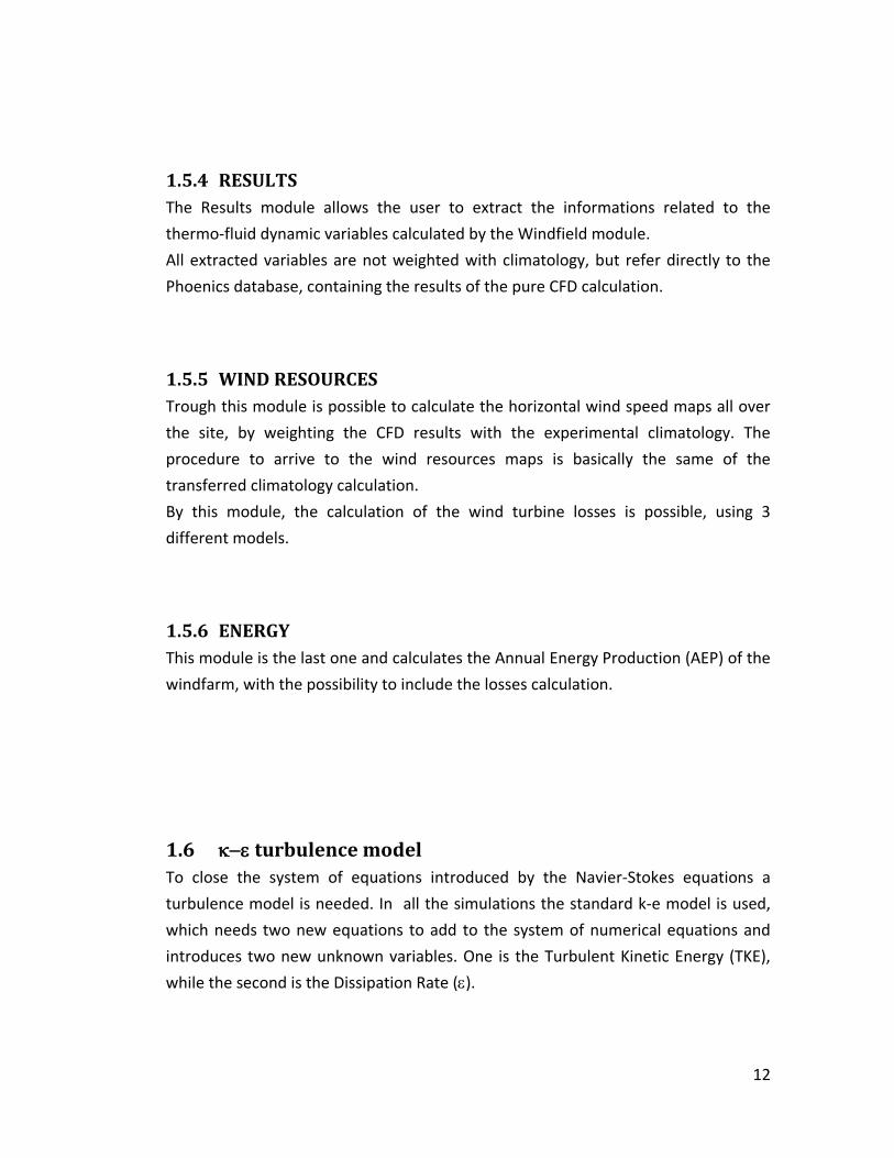
Figure 2.8: Vertical profiles for R=0.01 and 20 vertical cells.
Figure 2.9: Vertical profiles for R=0.3 and 20 vertical cells.

24
Figure 2.10: Vertical profiles for R=0.6 and 20 vertical cells.
As can be easily seen, the two boundary conditions at the top level produce
different results in the shape of the velocity profile. The most important effect is the
velocity variation during the flow development on the domain. According to the
neutral ABL, the velocity profile should not change along the domain, an this is the
case of figure 2.8 where a low value of roughness was imposed. The effect of profile
variation is amplified by the growth of the roughness value. This effect can be due to
numerical models used to close the RANS equation (turbulence model) and to
simulate the terrain roughness. In all the cases showed before, the effect of the
velocity deficit is more evident in simulations with zero pressure condition than in
simulations with the wall with no friction condition.
The second effect is the deformation of the velocity profile near the geostrophic
height. The zero pressure boundary condition produces in the exit station a velocity
profile that shows a maximum velocity similar to that of the inlet station. This fact,
together with the strong decrease of the axial velocity below the geostrophic height
leads to a diminution of the volume flow in the vertical stations along the domain.
As a results, the vertical component of the velocity increases and parte of the
volume flow exits from the top boundary condition, in contrast with the definition of
neutral ABL.

25
A different behavior is obtained when the wall with no friction BC is used. According
to the development of the boundary layer, the effects of the roughness slow down
along the domain and the velocity deficit between two stations decreases when
going toward the end of the flat terrain, confirming the general behavior of a
turbulent neutral ABL. Due to the particular boundary conditions the same volume
flow is maintained for all the vertical stations and the streamlines remain horizontal.
2.6 Remarks Flat terrains, like the model considered in this document, are not sensitive to the
increase of the vertical number of cells and then the default value (20 cells) seems
to be a good compromise between the goodness of the final results and the time
taken to run the simulation. An increase of the vertical cell number could be useful
in terrain with complex features.
The height distribution factor needs to be taken into account when, in region of the
flow attached to the terrain, a good precision is needed, and it should be decreased
slowly together with the increase of the horizontal resolution to avoid divergence
problems. From this analysis a limit value of the Height distribution factor was found
(HDF= 0.01).
The boundary condition to be assigned to the top level of the geometrical model has
been analyzed, showing that mass flow rate can be conserved only assigning the
wall with no friction boundary condition. This BC produces the effect of the shift of
the free stream velocity respect to the value superimposed in the WindSim module,
but the effect of velocity deficit due to the roughness value is strongly reduced,
mostly for high values of the roughness height.
26
CHAPTER 3. Simulations over 2D hilly terrains.
3.1 Introduction The present chapter concerns a series of numerical simulations on the behavior of
an air flow over a single hill, characterized by a roughness value on the ground. All
simulations have been run using a geometrical model in which a 3D “cos2” hill is
built: this fact causes the presence of a finite Y-dimension, generating 3D effects. To
avoid these errors can affect the results, all the simulations have been run
considering a very thin section of the 3D hill domain in Y-direction and the velocity
vertical profiles, needed for further analysis, have been extracted in the central cell
of the y-direction.
The results obtained in this way are totally equivalent to the results that could be
extracted by a “flatted” hill in y-direction, as illustrated in the next paragraph (figure
3.2), and they are not affected by tridimensional flow effects.
The shape of the speed vertical profiles along the hill has been also studied, and the
speed-up effect due to the variation of the terrain’s height has been highlighted.
Moreover, a sensitivity study of the numerical grid for hilly terrain has been carried
out, both for horizontal and vertical discretization.
Finally, a test case concerning the behavior of an air flow over a hilly terrain as been
reproduced: this case was good enough to put in evidence the separation
phenomena of the flow downstream the hill, and set some important parameters of
the WindSim software, to be used in complex terrains.
3.1.1 Similitude between a 3D “cos2” and “flatted” hill The following figure 3.1 shows the shape of the geometrical model in the X-Z plane
used to study the speed-up effect. The measurement stations, where speed vertical
profiles have been extracted, are also visualized.

27
Figure 3.1: Measurement stations of the speed vertical profiles.
The length of the model is 6000 m in X-direction, while the width is 75 m in Y-
direction. The number of cells is 240 X 3, for an equally spaced horizontal
discretization of 25 m. The height of the model is 1000 m and the vertical Z-direction
contains 20 cells; the Height Distribution Factor is 0,1 that means the first cell height
is equal to 9 m.
The hill shape has height H=100 m and half-length L=400 m, while the top is
centered at a distance of 2000 m from inlet section.
Figure 2: Sketch of the numerical domain of the 2D hill.
In the following table 3.1 the coordinates of the measurement points are reported.

28
Table 3.1: Measurement coordinates
Station X [m] Y [m]
0 0 37,5 1 1000 37,5 2 1300 37,5 3 1600 37,5 4 1800 37,5 5 1900 37,5 6 2000 37,5 7 2100 37,5 8 2200 37,5 9 2400 37,5
10 3700 37,5 11 3000 37,5 12 4000 37,5 13 6000 37,5
The height of the model is 1000 m from the ground level and the top surface contain
the wall with no-friction boundary condition, studied in the previous chapter. The
geostrophic wind is standing at 500 m with a free stream velocity equal to 10 m/s.
The description of the model is completed with the following figure 3.2, showing the
difference in the profile of the hill obtained with a section of the Y-Z plane, between
a “cos2” and a “flatted” hill.
Figure 3.2: View of the geometrical models “cos2” and “flatted” hill from the inlet sections.
The “cos2” hill has been built through the automatic procedure of the WindSim
software, which draws the hill shape using the following equation.

3.1.1)
while the flatted one has been created manually by the same 3D equation projected
in the X-Z plane.
The simulations have been run using the standard
coupled solver. The velocity vertical profiles have been calculated in some of the
stations shown in figure 3.1 and the results of the comparison are reported in the
following figures 3.3.
3.1.1)
while the flatted one has been created manually by the same 3D equation projected
Z plane.
The simulations have been run using the standard
coupled solver. The velocity vertical profiles have been calculated in some of the
stations shown in figure 3.1 and the results of the comparison are reported in the
following figures 3.3.
Figure 3.3: Overlay of the vertical profiles in some measurement stations.
,
while the flatted one has been created manually by the same 3D equation projected
The simulations have been run using the standard κ−ε turbulence model and the
coupled solver. The velocity vertical profiles have been calculated in some of the
stations shown in figure 3.1 and the results of the comparison are reported in the
l profiles in some measurement stations.
29
while the flatted one has been created manually by the same 3D equation projected
turbulence model and the
coupled solver. The velocity vertical profiles have been calculated in some of the
stations shown in figure 3.1 and the results of the comparison are reported in the

The results shown above demonstrate that the vertical profiles extracted from the
central cell in the Y
a “flatted” Y
effect on the flow. This is a striking result, and it is useful for further simulations,
because it’s demonstrated that a very thin 3D “cos
procedure of the WindSim software, can b
air flow over a 2D hill.
3.2 SpeedThe speed
value of the roughness height. Particularly, 3 tests have been done, for R=0,01 m ,
R=0,3 m and R=0,6 m.
The following picture shows the development of the speed vertical profiles
measured in the various stations, upstream and downstream the hill top (located in
station number 6).
The results shown above demonstrate that the vertical profiles extracted from the
central cell in the Y-direction of a 3D “cos2
a “flatted” Y-direction hill, which doesn’t
effect on the flow. This is a striking result, and it is useful for further simulations,
because it’s demonstrated that a very thin 3D “cos
procedure of the WindSim software, can b
air flow over a 2D hill.
Speed-up effect The speed-up effect has been studied for the case shown in figure 3.1, varying the
value of the roughness height. Particularly, 3 tests have been done, for R=0,01 m ,
3 m and R=0,6 m.
The following picture shows the development of the speed vertical profiles
measured in the various stations, upstream and downstream the hill top (located in
station number 6).
Figure 3.4: Development of the vertical profiles upstream t
The results shown above demonstrate that the vertical profiles extracted from the 2” hill are the same as those extracted from
direction hill, which doesn’t introduce therefore any tri-dimensional
effect on the flow. This is a striking result, and it is useful for further simulations,
because it’s demonstrated that a very thin 3D “cos2” hill, built up with the automatic
procedure of the WindSim software, can be used to understand the behavior of an
up effect has been studied for the case shown in figure 3.1, varying the
value of the roughness height. Particularly, 3 tests have been done, for R=0,01 m ,
The following picture shows the development of the speed vertical profiles
measured in the various stations, upstream and downstream the hill top (located in
Figure 3.4: Development of the vertical profiles upstream the hill-top.
30
The results shown above demonstrate that the vertical profiles extracted from the
” hill are the same as those extracted from
dimensional
effect on the flow. This is a striking result, and it is useful for further simulations,
” hill, built up with the automatic
e used to understand the behavior of an
up effect has been studied for the case shown in figure 3.1, varying the
value of the roughness height. Particularly, 3 tests have been done, for R=0,01 m ,
The following picture shows the development of the speed vertical profiles
measured in the various stations, upstream and downstream the hill top (located in
Starting from station 0, the flow is slowing down until station 2: this behavior is
caused by the effect of the roughness (as explained in chapter 2). Between station
and station 3 the slowing effect is stronger, due to the presence of the obstacle (the
hill). When the flow passes over station 3, the hill geometry accelerates the flow,
like in a subsonic convergent duct. The speed increase is registered until the top
the hill, where the horizontal speed gets the maximum value.
When the flow passes over station 6 (hill top), it sees a subsonic divergent duct and
the effect of slow down begins and continues until station 9.
tends to increase the
the flow starts to accelerate again, in order to get the initial conditions.
A similar behavior of the flow over a hilly terrain can be found i
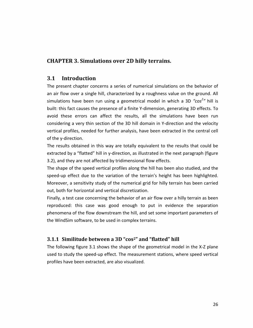
Figure 3.5: Development of the vertical profiles downstream the hill
Starting from station 0, the flow is slowing down until station 2: this behavior is
caused by the effect of the roughness (as explained in chapter 2). Between station
and station 3 the slowing effect is stronger, due to the presence of the obstacle (the
hill). When the flow passes over station 3, the hill geometry accelerates the flow,
like in a subsonic convergent duct. The speed increase is registered until the top
the hill, where the horizontal speed gets the maximum value.
When the flow passes over station 6 (hill top), it sees a subsonic divergent duct and
the effect of slow down begins and continues until station 9.
tends to increase the boundary layer more than the starting value.
the flow starts to accelerate again, in order to get the initial conditions.
A similar behavior of the flow over a hilly terrain can be found i
Figure 3.5: Development of the vertical profiles downstream the hill-top.
Starting from station 0, the flow is slowing down until station 2: this behavior is
caused by the effect of the roughness (as explained in chapter 2). Between station
and station 3 the slowing effect is stronger, due to the presence of the obstacle (the
hill). When the flow passes over station 3, the hill geometry accelerates the flow,
like in a subsonic convergent duct. The speed increase is registered until the top
the hill, where the horizontal speed gets the maximum value.
When the flow passes over station 6 (hill top), it sees a subsonic divergent duct and
the effect of slow down begins and continues until station 9. The divergent channel
boundary layer more than the starting value. Then gradually,
the flow starts to accelerate again, in order to get the initial conditions.
A similar behavior of the flow over a hilly terrain can be found in [2]
31
Starting from station 0, the flow is slowing down until station 2: this behavior is
caused by the effect of the roughness (as explained in chapter 2). Between station 2
and station 3 the slowing effect is stronger, due to the presence of the obstacle (the
hill). When the flow passes over station 3, the hill geometry accelerates the flow,
like in a subsonic convergent duct. The speed increase is registered until the top of
When the flow passes over station 6 (hill top), it sees a subsonic divergent duct and
The divergent channel
Then gradually,

32
Figure 3.6: Sketch of the 15 km long hilly terrain model.
A longer model described in figure 3.6 has been studied to highlight the behavior of
the vertical profiles in the far region downstream the hill top. As it can be seen from
figures 3.7 the vertical profile of the flow seems to be fully developed in station 22,
in a distance 13 km away downstream the hill top.
Figure 3.7: Vertical profiles extracted in the downstream flat area of the model.
The simulations run for R=0,3 m and for R=0,6 m show similar behavior of the speed
up effect. The effect of the roughness height is stronger than that of the first
simulation, and this fact induces a different growth of the boundary layer thickness,
as shown in the figure 3.8.
33
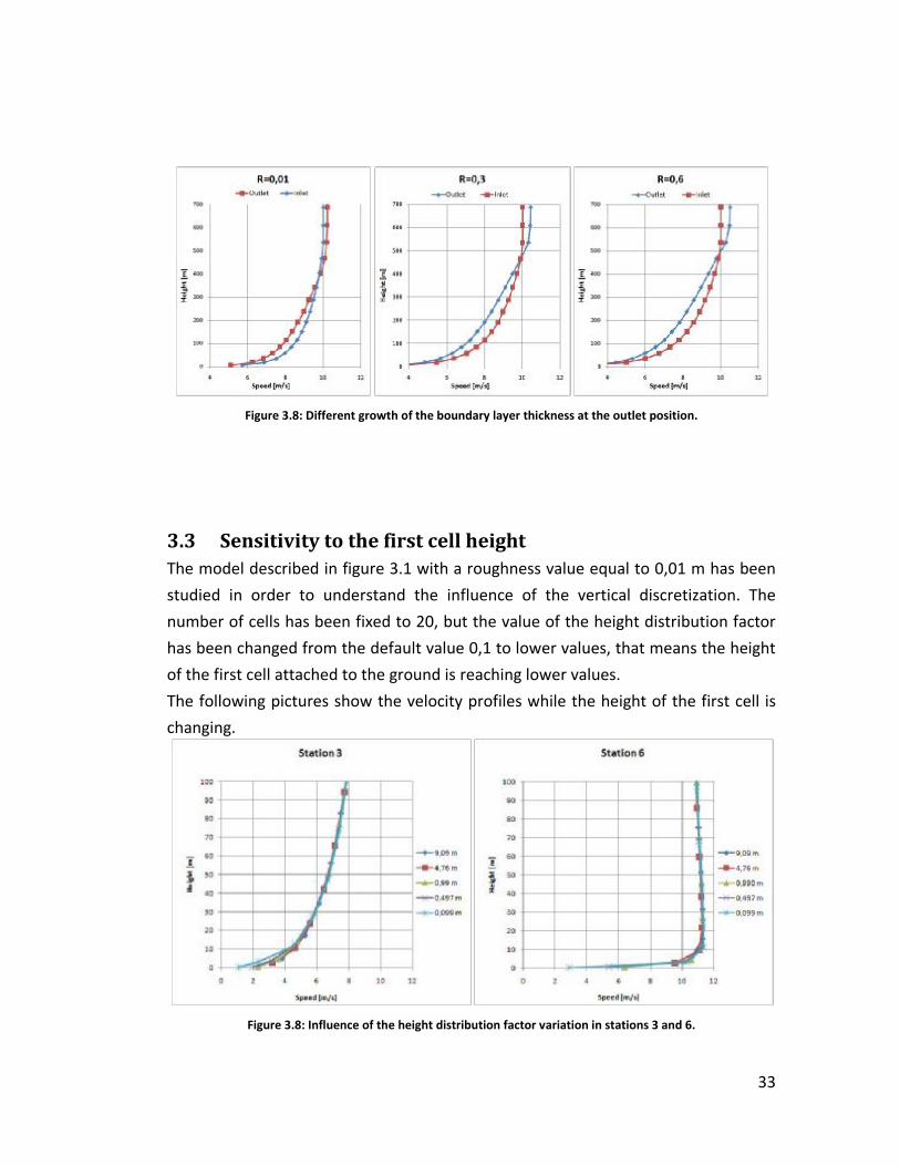
Figure 3.8: Different growth of the boundary layer thickness at the outlet position.
3.3 Sensitivity to the first cell height The model described in figure 3.1 with a roughness value equal to 0,01 m has been
studied in order to understand the influence of the vertical discretization. The
number of cells has been fixed to 20, but the value of the height distribution factor
has been changed from the default value 0,1 to lower values, that means the height
of the first cell attached to the ground is reaching lower values.
The following pictures show the velocity profiles while the height of the first cell is
changing.
Figure 3.8: Influence of the height distribution factor variation in stations 3 and 6.
34
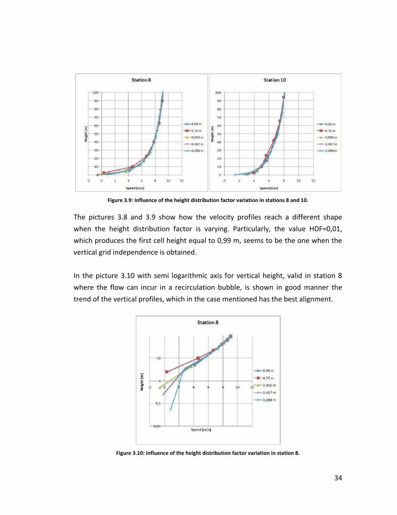
Figure 3.9: Influence of the height distribution factor variation in stations 8 and 10.
The pictures 3.8 and 3.9 show how the velocity profiles reach a different shape
when the height distribution factor is varying. Particularly, the value HDF=0,01,
which produces the first cell height equal to 0,99 m, seems to be the one when the
vertical grid independence is obtained.
In the picture 3.10 with semi logarithmic axis for vertical height, valid in station 8
where the flow can incur in a recirculation bubble, is shown in good manner the
trend of the vertical profiles, which in the case mentioned has the best alignment.
Figure 3.10: Influence of the height distribution factor variation in station 8.
35
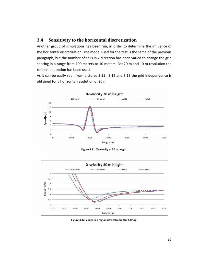
3.4 Sensitivity to the horizontal discretization Another group of simulations has been run, in order to determine the influence of
the horizontal discretization. The model used for the test is the same of the previous
paragraph, but the number of cells in x-direction has been varied to change the grid
spacing in a range from 100 meters to 10 meters. For 20 m and 10 m resolution the
refinement option has been used.
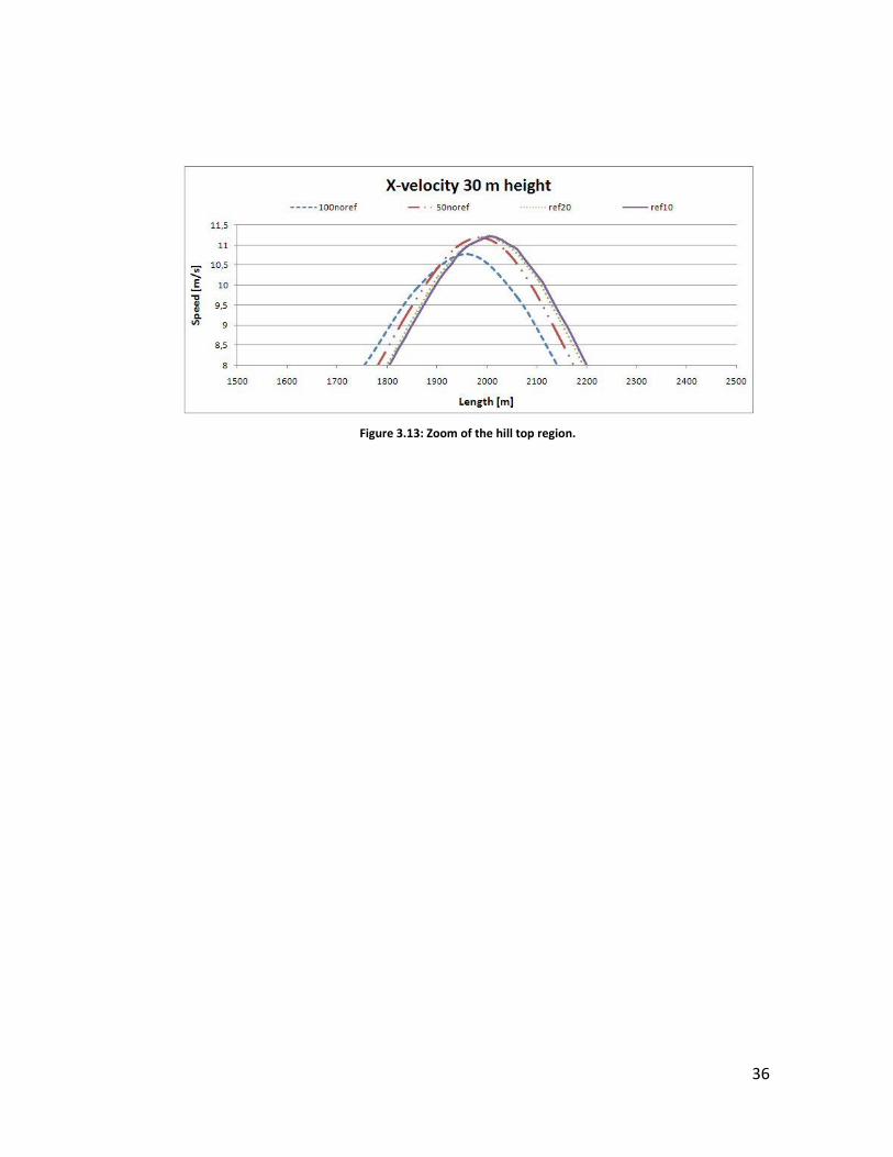
As it can be easily seen from pictures 3.11 , 3.12 and 3.13 the grid independence is
obtained for a horizontal resolution of 20 m
Figure 3.11: X-velocity at 30 m height.
Figure 3.12: Zoom in a region downstream the hill top.
36
Figure 3.13: Zoom of the hill top region.

37
3.5 Investigation of a flow over a 2D roughly hilly terrain This paragraph presents an investigation of a flow over a two–dimensional roughly
hilly terrain. Two cases have been realized, to highlight the behavior of an attached
flow and a separated flow, by varying the slope of the hill. A comparison between
experimental [3] and numerical data has been done, showing good agreement.
The numerical simulations are based on the solution of Reynolds Averaged Navier-
Stokes (RANS) equations, by the software WindSim, with the k-ε turbulence
model. The realized numerical grid is in both cases non orthogonal body fitted type,
while the solver which better produces a good level of convergence in the solution is
the segregated, enriched with the “yap” correction of the k-ε turbulence model.
3.5.1 Description of the test case The experimental data comes from the tests conducted in an open-circuit boundary-
layer wind tunnel, having a test section of width, height and length of 1.2, 1.2 and 6
meters respectively. A neutrally stratified boundary layer is developed using equally
spaced 0.25 m height triangular spire-type vortex generators and artificial grass of 5
mm height. In these experiments, a fully-developed turbulent boundary layer of 0.25
m height is generated, and has a typical wind profile over an open flat area (fitting to
a log-law profile).
The shape of the hill is described by the following equation
3.5.1) = ∙ 1 + ∙ ,
where:
H [m] is the height of the hill
L1 [m] is the half-length of the hill at the upwind mid-height of the
hill
The slope of the hill S is defined as the average slope for the top half of the hill
upstream of the crest, through the equation

38
3.5.2) = ∙ .
The two models for attached and separated flow are identified as S3H4 and S5H4,
where S3 and S5 stand for the hill slope of 0.3 and 0.5 respectively, and H4 stand for
the hill height of 4 centimeters.
A sketch of the studied hill is presented in the following figure 3.5.1
Figure 3.14: Schematic diagram of the wind flow over a hill.
The experimental data, relative to the flow at the inlet of the wind tunnel, have been curve-fitted with the following logarithmic function
3.5.3) ( ) = ∗ ∙
with:
U*=0,33 m/s
Z0=0,05 mm
K=0,41 Von Karman constant
The following figure 3.15 shows the interpolation of the velocity profile.

39
Figure 3.15: Mean velocity profile over the flat floor at inlet position.
3.5.2 Numerical method The WindSim software solves the RANS equations (Reynolds Averaged Navier
Stokes), using the finite volume method through a graphical interface and the CFD
solver Phoenics. The continuity equation and the three momentum equations are
solved, using the standard k-ε turbulence model to introduce the equations
needed to solve the Reynolds stress tensor.
Also the “Yap” correction for k-ε turbulence model is needed to help the
convergence process in the separated flow. In addition to the turbulence model, the
wall function is imposed to the ground.
The fluid blown by the wind tunnel is air, in incompressible flow condition: in this
way, no thermal effects are present. The characteristic of this flow is expressed by
the Reynolds Number, defined as
3.5.4) = ∙ = 1,87 × 10
where:
U∞ [m/s] free stream velocity

40
H [m] hill height ν [m2/s] air cinematic viscosity
The numerical grid is built, in both S3H4 and S5H4 cases, with a non-orthogonal grid
as shown in the further paragraphs.
3.5.3 Case S3H4 The case S3H4 has been studied in a geometrical model extending from streamwise
coordinates -1,5 m to 1,5 m, for a total length of 3 m. The width is 0,1 m while the
total height is 2 m; thus, the blockage factor is 2%.
The grid contains 130 cells in x-directions, 3 cells in y-direction and 60 cells in
vertical direction; the horizontal resolution has been increased in the hill profile, in
order to describe in a sufficient accurate way the behavior of the flow in the critical
zone. The height of the first cell is 2 mm, while the roughness height imposed in the
wall function formula is 0,05 mm. Then, the condition stating that the first cell
height must be at least double of the roughness value is satisfied [1].
The following figure 3.16 shows a particular of the numerical grid.
Figure 1.16: Particular of the non-orthogonal regular grid for case S3H4.
The boundary condition imposed on the top of the model is “wall with no-friction”,
while at the bottom the terrain contains the roughness information all over the
surface.

41
At the inlet, the vertical profile of velocity is imposed, with the log law reaching a
speed of 7 m/s, to keep the same Reynolds Number of the experiments, at 0,28 m
height.
To run the simulation, a segregated solver (SIMPLEST) has been used, with a number
of iterations equal to 1000.
The picture below shows the residual values of the variables solved by WindSim.
Figure 3.17: Residual values for case S3H4.
3.5.4 Case S5H4 The case S5H4 has been created keeping the same original dimensions of the case
S3H4.
Due to the shape of the hill, steeper than case S3H4, the number of horizontal cells
has been grown up to 150, to obtain a total number of cell equal to 2700. The height
of the first cell is still 2 mm, while the roughness value of the terrain is 0,05 mm.
Also in this case, the height of the first cell is higher than the two times the value of
the roughness height. Concerning the boundary conditions, the top of the model is
set as “wall with no-friction”.

42
Figure 3.18: Particular of the numerical grid for case S5H4.
To run the simulation, the segregated solver option has been used, with a number of
iterations equal to 2000. The “Yap” correction [5] for turbulence model has also
been used in this case, to help the convergence process in a flow supposed to be
separated.
Figure 3.19: Residual values for case S5H4.

43
3.5.5 Results
Case S3H4
The following images show the solution of the flow field for the case S3H4. Figure
3.20 show the 2D speed scalar value calculated all over the model, while figure 3.21
shows the vertical velocity component, due to the shape of the terrain.
Figure 3.20: Speed 2D.
Figure 3.21: Z velocity component.

44
Finally, the horizontal x velocity component has been shown in the figure 3.22, in
order to show the region of the model in which the recirculation of the flow can
occur.
Figura 3.22: X velocity component.
The following figure 3.23 shows the comparison between experimental data,
marked with the circle, and the results of the simulation, marked with the solid line.
The solid circles laying on the ground line refer to the measurement points.

45
Figure 3.23: Comparison between experimental and numerical data.
Case S5H4
As well as in the previous case, the pictures below show the 2D speed scalar
distribution, the vertical velocity component and the horizontal x velocity.
Figure 3.24: Speed 2D.

46
Figure 3.25: Z velocity component
Figura3.26: X velocity component.
47
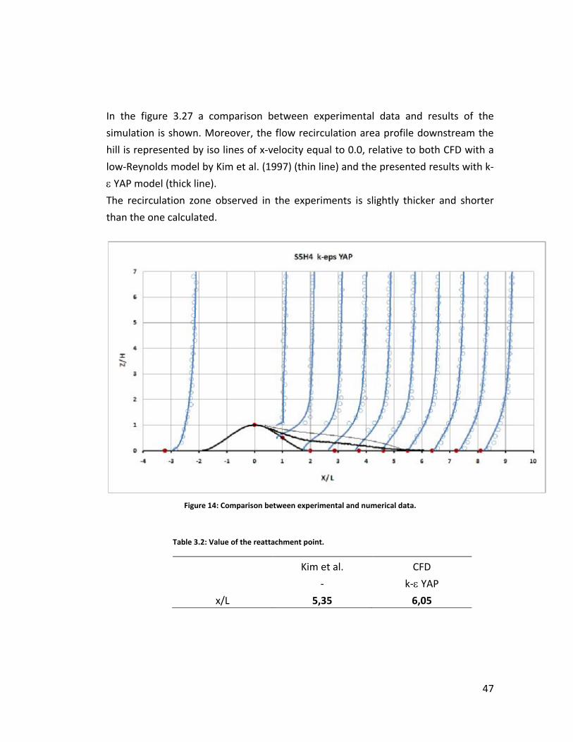
In the figure 3.27 a comparison between experimental data and results of the
simulation is shown. Moreover, the flow recirculation area profile downstream the
hill is represented by iso lines of x-velocity equal to 0.0, relative to both CFD with a
low-Reynolds model by Kim et al. (1997) (thin line) and the presented results with k-
ε YAP model (thick line).
The recirculation zone observed in the experiments is slightly thicker and shorter
than the one calculated.
Figure 14: Comparison between experimental and numerical data.
Table 3.2: Value of the reattachment point.
Kim et al. CFD
- k-ε YAP
x/L 5,35 6,05

48
3.6 Remarks A CFD study of a boundary layer flow over 2D rough hills has been performed. The
aim of the presented simulations was to reproduce the experimental wind tunnel
results by Kim et al. (1997), and set the parameters of WindSim to run in presence of
hilly terrains. Both the experimental and numerical results show the different
behaviors of the flow depending on the shape of the hill. Moreover, both the hills
with slope S 0,3 and S 0,5 cause a separation of the flow, generating a recirculation
area downstream of the hill.
The case S5H4 shows a good agreement between experimental and numerical
results. The performed simulation over predicts the length of the separated area by
13%; the overestimation of the recirculation zone is probably due to the usage of
the YAP correction [5] for the k-ε closure. The k-ε model coupled with the hybrid
discretization scheme on a BFC grid would estimate a recirculation bubble smaller
than the one of the experiments, according to the conclusions by Kim et al. (1997) .
To solve this case, the segregated solver was good enough to reproduce the
behavior of the flow. The turbulence has been modeled with a standard k-ε model
and the “Yap” correction has been used.
Concerning the case S3H4, in which separation has not been observed in the
experiments, a very small recirculation zone appeared in the numerical results, in
the region downstream of the hill.
This fact should be linked to the turbulence level of the flow set at the inlet of the
tunnel: the modification of the turbulence intensity is not allowed in WindSim when
setting the inlet boundary condition; then, it’s possible that in this simulation the
turbulence level wasn’t high enough to maintain the flow attached to the terrain.
Anyway, no specification on the turbulence level was found in the reference [2] for
this very complex case, which has been observed to be at the boundary between the
attached flow and occurrence of separation.
In all cases a segregated solver with the “Yap” correction for k-ε turbulence model
was also needed to produce a good convergence of the field variables.

49
CHAPTER 4. Characteristics of the site.
4.1 Introduction The site studied in this document is located in a region of Central Italy and is visible
in the following satellite image.
Figure 4.1: Aerial picture of the Antrodoco site.
It can be seen that the region is in a mountain area, covered by thick forest for a
wide zone. Rocks and stones are also present with some agricultural plowed areas.
Two roads are signed in the maps, running along the valley colored in yellow.
Moreover, some urban areas are found in the zone, mostly small mountain villages;
one of this is an important town, in proximity of the conjunction of the two roads.
50
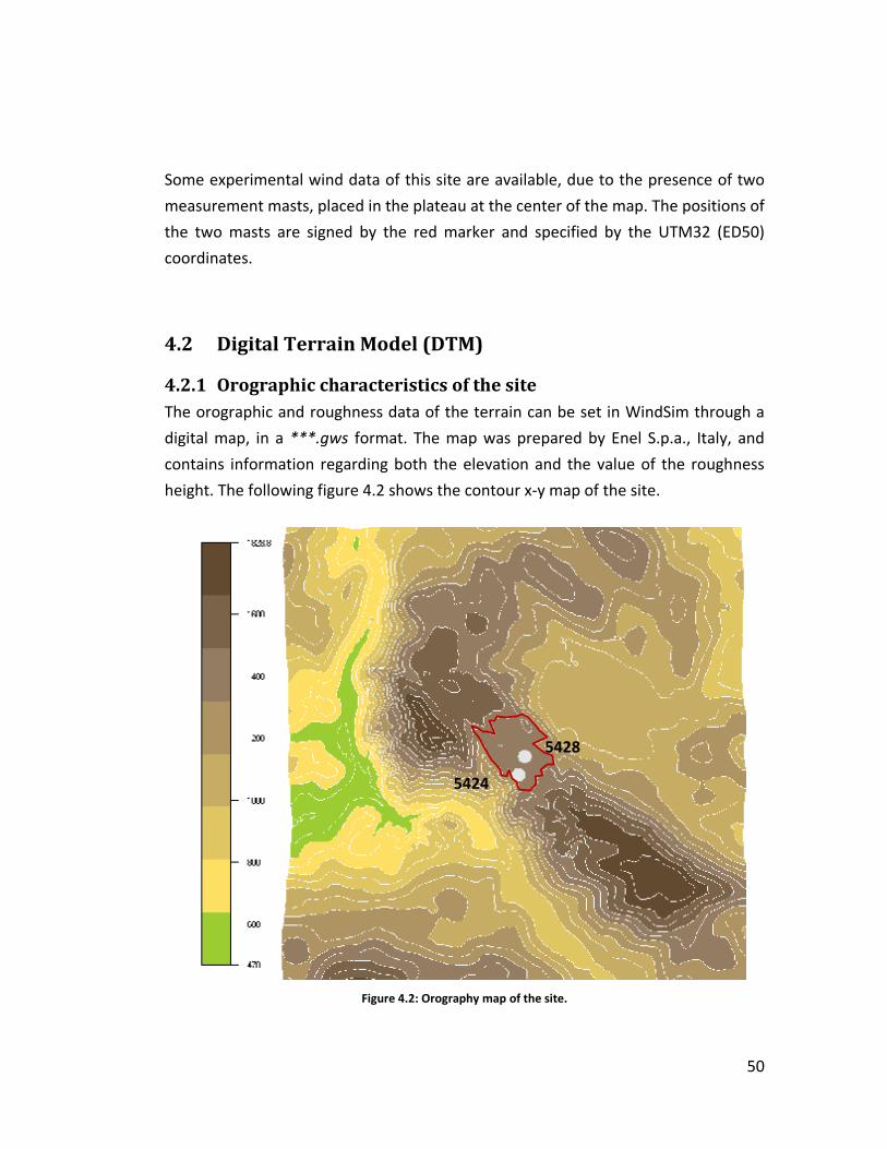
Some experimental wind data of this site are available, due to the presence of two
measurement masts, placed in the plateau at the center of the map. The positions of
the two masts are signed by the red marker and specified by the UTM32 (ED50)
coordinates.
4.2 Digital Terrain Model (DTM)
4.2.1 Orographic characteristics of the site The orographic and roughness data of the terrain can be set in WindSim through a
digital map, in a ***.gws format. The map was prepared by Enel S.p.a., Italy, and
contains information regarding both the elevation and the value of the roughness
height. The following figure 4.2 shows the contour x-y map of the site.
Figure 4.2: Orography map of the site.
5428
5424
51
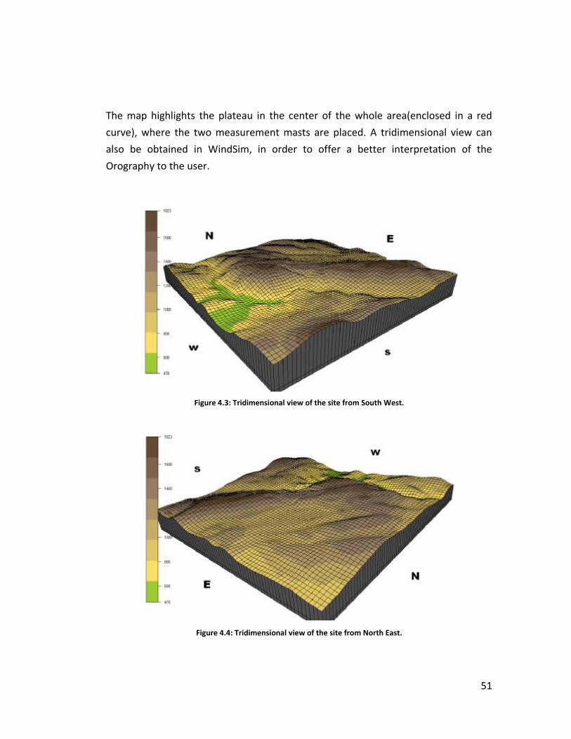
The map highlights the plateau in the center of the whole area(enclosed in a red
curve), where the two measurement masts are placed. A tridimensional view can
also be obtained in WindSim, in order to offer a better interpretation of the
Orography to the user.
Figure 4.3: Tridimensional view of the site from South West.
Figure 4.4: Tridimensional view of the site from North East.

52
Both the pictures 4.3 and 4.4 have been built and colored maintaining the same
height scale which ranges from 470 m to 1823 m.
Notice that in direction NE-SW the quote of the terrain grows very slowly to the top
of the rocky mountain. Over the top, a deep valley is present, where the step
between the maximum and the minimum height is in order of 1400 meters.
4.2.2 Roughness characteristics The whole area has been subdivided into three main roughness regions,
characterized by three different values of roughness heights. The roughness classes
are explained in the table 4.1.
Table 4.1: Roughness values assigned to the site.
DESCRIPTION Z0 [m]
Rocks, stones an plowed terrain 0,03
Forest 0,65
Urban areas 0,80
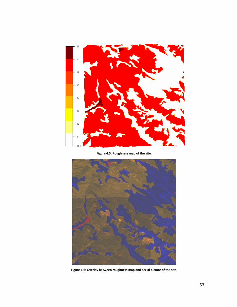
The figure 4.5 represents the roughness contour map of the region.
The plateau is all characterized by a roughness value of Z0 = 0,03 m ; in fact no trees
and other kind of vegetation is present in this region.
The Windsim software allows the comparison of the actual contour map of
roughness with a satellite aerial picture of the site. The result of this procedure is
reported in the further figure 4.6.
To allow the overlay, in the roughness colors with paints that contrast the typical
colors of a satellite picture are used in the figure and listed in table 4.2.
53
Figure 4.5: Roughness map of the site.
Figure 4.6: Overlay between roughness map and aerial picture of the site.

54
Table 4.2: Description of the colors used in the overlaid map.
DESCRIPTION COLOR
Rocks, stones and plowed terrain Blue
Forest Transparent
Urban areas Red
The analysis of the previous picture shows a good agreement between the
roughness map and the satellite picture, demonstrating that the whole area is well
described. Anyhow, there is evidence of some particular zones which are not exactly
described by the contour lines. In fact, the yellow color of the picture (relative to the
satellite image) should be totally covered by the blue color (relative to the
roughness map), equal to Z0 = 0,03 m.
Some disagreement in the zones far from the plateau is not important and errors in
the roughness should not influence in a strong way the final results in the area of
interest. Nevertheless, the better the area very close to the plateau is described the
more precise the result are.
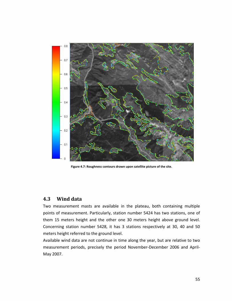
A more detailed comparison between the two maps can be accomplished by the
image 4.7, showing the roughness contours drawn upon the satellite image at the
maximum possible resolution (30 meters).
It is confirmed that some zones are not covered by vegetation as conversely
represented in the roughness map. Despite of this slight disagreement, the
roughness map has not been modified.
Finally, a further consideration should be done: the satellite map, extracted from
Google Earth software, can contain irregularities and be some years old.
55
Figure 4.7: Roughness contours drawn upon satellite picture of the site.
4.3 Wind data Two measurement masts are available in the plateau, both containing multiple
points of measurement. Particularly, station number 5424 has two stations, one of
them 15 meters height and the other one 30 meters height above ground level.
Concerning station number 5428, it has 3 stations respectively at 30, 40 and 50
meters height referred to the ground level.
Available wind data are not continue in time along the year, but are relative to two
measurement periods, precisely the period November-December 2006 and April-
May 2007.

56
In this periods, data are recorded by the anemometer’s data logger, and stored in a
data file like the one shown in table 4.3, where data are averaged in a 10 minutes
period.
The figure 4.8 show the 3 cup NRG #40 anemometer and the NRG #200P wind
direction vane used to measure the wind characteristics. Detailed informations
about their technical specifications can be found in bibliography [8].
Figure 4.8: NRG #40 anemometer and NRG #200P wind direction vane.
Table 4.3: Example of a wind data file.
Day Month Year Hour Minute Mean speed Max speed Standard
deviation
Direction Standard
deviation
- - - [H] [min] [m/s] [m/s] [m/s] [degree] [degree]
1 4 2007 0 30 0,3 2,0 0,5 74 2
1 4 2007 0 40 0,8 1,5 0,5 75 0
1 4 2007 0 50 0,9 1,5 0,3 75 0
1 4 2007 0 60 1,3 2,0 0,2 75 0
1 4 2007 1 10 1,6 2,3 0,3 70 8
1 4 2007 1 20 1,8 2,3 0,3 73 18

57
Figures 4.9 and 4.10 show a 3D representation of the two measurement stations,
the position and display the orography of the terrain close to them.
Figure 4.9: Site position of the mast measurement. View from South-West.
Figure 4.10: Site position of the mast measurement. View from East.
5424
5428
5424
5428

58
In the following pages, a short description of every single data set is presented,
reporting the wind frequency rose and the main results which describe the Weibull
fitting of the recorded data.
All experimental data have been filtered, eliminating the errors recorded by the data
logger during bad working of the anemometer.
Moreover, the dominant sectors have been highlighted in yellow; referring to the
other sectors, the ones which frequency is below 1,5 % have been highlighted in
green, in order to facilitate the understanding of the processed WindSim results,
presented in chapter 6.
In these sectors the calculated statistic parameters are not good enough because
the number of samples used to analyze them is low.

59
4.3.1 Mast 5424-30 m Period April-May 2007
Table 4.4: Weibull (k,A), frequency (-) and average wind speed (m/s) versus sector.
5424-30 April-May
0 30 60 90 120 150 180 210 240 270 300 330
k 2,4 2,42 2,59 1,32 1,08 0,77 0,91 1,4 2,57 0,84 0,64 1,51
A 4,1 5,95 6 2,6 1,31 0,94 1,57 5,46 7,29 1,09 0,57 3
freq 0,034 0,299 0,17 0,011 0,01 0,009 0,026 0,303 0,128 0,006 0,003 0,005
mean 3,39 5,12 5,12 2,33 1,27 1,33 1,73 4,63 5,93 1,34 1,15 2,59
Figure 4.11: Frequency of records and Weibull fitting.
RESULTS
Total records 8614
Average wind speed 4,79 m/s
Shape parameter K 1,84
Scale parameter A 5,77 m/s
Median 4,73 m/s
Mode 3,77 m/s

60
4.3.2 Mast 5424-15 m Period April-May 2007
Table 4.5: Weibull (k,A), frequency (-) and average wind speed (m/s) versus sector.
5424-15 April-May
0 30 60 90 120 150 180 210 240 270 300 330
k 1,95 2,6 2,23 0,85 0,87 0,69 0,72 1,75 2,4 1,26 0,72 1,8
A 3,87 6,15 5,1 1,03 0,77 0,56 0,76 5,82 6,84 1,28 0,77 2,73
freq 0,034 0,354 0,123 0,012 0,01 0,01 0,05 0,328 0,072 0,003 0,003 0,003
mean 3,18 5,23 4,27 1,27 0,92 0,93 1,15 4,86 5,63 1,23 1,2 2,3
Figure 4.12: Frequency of records and Weibull fitting.
RESULTS
Total records 8614
Average wind speed 4,59 m/s
Shape parameter K 1,93
Scale parameter A 5,58 m/s
Median 4,61 m/s
Mode 3,82 m/s

61
4.3.3 Mast 5424-30 m Period November-December 2006
Table 4.6: Weibull (k,A), frequency (-) and average wind speed (m/s) versus sector.
5424-30 November-December
0 30 60 90 120 150 180 210 240 270 300 330
k 2,15 2 1,92 0,75 1,82 1,04 1,1 1,31 1,32 1,13 0,71 0,74
A 4,04 6,32 7,08 0,89 0,71 1,05 2,69 5,11 4,71 0,73 0,63 0,67
freq 0,026 0,17 0,202 0,01 0,01 0,007 0,032 0,436 0,097 0,007 0,004 0,006
mean 3,35 5,47 6,01 1,2 0,63 1,15 2,61 4,59 4,24 0,68 1,05 1,03
Figure 4.13: Frequency of records and Weibull fitting.
RESULTS
Total records 8240
Average wind speed 4,76 m/s
Shape parameter K 1,45
Scale parameter A 5,43 m/s
Median 4,22 m/s
Mode 2,42 m/s
62
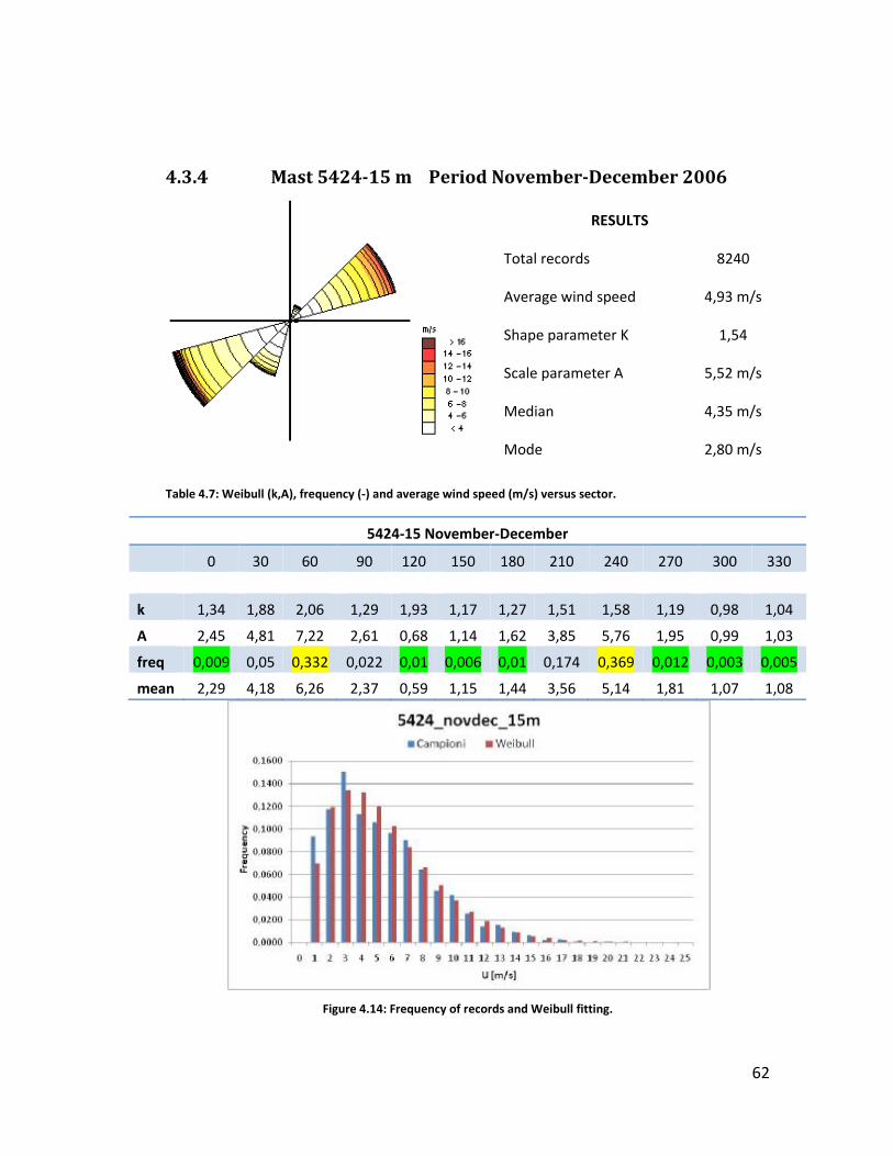
4.3.4 Mast 5424-15 m Period November-December 2006
Table 4.7: Weibull (k,A), frequency (-) and average wind speed (m/s) versus sector.
5424-15 November-December
0 30 60 90 120 150 180 210 240 270 300 330
k 1,34 1,88 2,06 1,29 1,93 1,17 1,27 1,51 1,58 1,19 0,98 1,04
A 2,45 4,81 7,22 2,61 0,68 1,14 1,62 3,85 5,76 1,95 0,99 1,03
freq 0,009 0,05 0,332 0,022 0,01 0,006 0,01 0,174 0,369 0,012 0,003 0,005
mean 2,29 4,18 6,26 2,37 0,59 1,15 1,44 3,56 5,14 1,81 1,07 1,08
Figure 4.14: Frequency of records and Weibull fitting.
RESULTS
Total records 8240
Average wind speed 4,93 m/s
Shape parameter K 1,54
Scale parameter A 5,52 m/s
Median 4,35 m/s
Mode 2,80 m/s
63
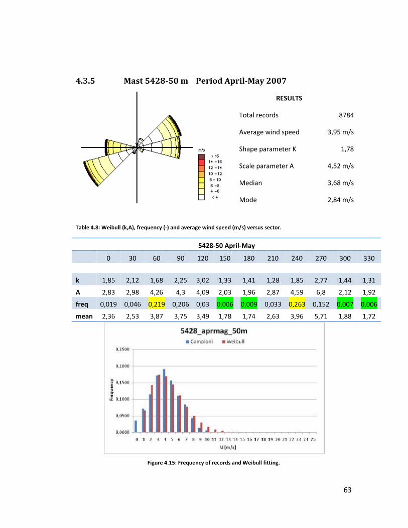
4.3.5 Mast 5428-50 m Period April-May 2007
Table 4.8: Weibull (k,A), frequency (-) and average wind speed (m/s) versus sector.
5428-50 April-May
0 30 60 90 120 150 180 210 240 270 300 330
k 1,85 2,12 1,68 2,25 3,02 1,33 1,41 1,28 1,85 2,77 1,44 1,31
A 2,83 2,98 4,26 4,3 4,09 2,03 1,96 2,87 4,59 6,8 2,12 1,92
freq 0,019 0,046 0,219 0,206 0,03 0,006 0,009 0,033 0,263 0,152 0,007 0,006
mean 2,36 2,53 3,87 3,75 3,49 1,78 1,74 2,63 3,96 5,71 1,88 1,72
Figure 4.15: Frequency of records and Weibull fitting.
RESULTS
Total records 8784
Average wind speed 3,95 m/s
Shape parameter K 1,78
Scale parameter A 4,52 m/s
Median 3,68 m/s
Mode 2,84 m/s

64
4.3.6 Mast 5428-40 m Period April-May 2007
Table 4.9: Weibull (k,A), frequency (-) and average wind speed (m/s) versus sector.
5428-40 April-May
0 30 60 90 120 150 180 210 240 270 300 330
k 2,05 2,27 1,83 2,39 3,22 1,43 1,5 1,29 1,91 2,82 1,51 1,18
A 3,12 3,05 4,04 4,09 3,98 1,92 1,87 2,88 4,6 6,76 2,26 1,66
freq 0,019 0,046 0,219 0,206 0,03 0,006 0,009 0,033 0,263 0,152 0,007 0,006
mean 2,59 2,61 3,64 3,58 3,4 1,7 1,63 2,65 3,96 5,68 1,93 1,59
Figure 4.16: Frequency of records and Weibull fitting.
RESULTS
Total records 8784
Average wind speed 3,86 m/s
Shape parameter K 1,80
Scale parameter A 4,40 m/s
Median 3,59 m/s
Mode 2,80 m/s

65
4.3.7 Mast 5428-30 m Period April-May 2007
Table 4.10: Weibull (k,A), frequency (-) and average wind speed (m/s) versus sector.
5428-30 April-May
0 30 60 90 120 150 180 210 240 270 300 330
k 1,87 2,15 2,03 2,57 3,33 1,3 1,55 1,32 1,92 2,85 1,57 1,19
A 2,66 2,62 3,7 3,82 3,85 1,72 1,82 2,71 4,4 6,56 2,25 1,66
freq 0,019 0,046 0,219 0,206 0,03 0,006 0,009 0,033 0,263 0,152 0,007 0,006
mean 2,24 2,24 3,26 3,33 3,28 1,56 1,6 2,46 3,79 5,52 1,91 1,57
Figure 4.17: Frequency of records and Weibull fitting.
RESULTS
Total records 8784
Average wind speed 3,62 m/s
Shape parameter K 1,78
Scale parameter A 4,13 m/s
Median 3,36 m/s
Mode 2,60 m/s

66
4.3.8 Mast 5428-50 m Period November-December 2006
Table 4.11: Weibull (k,A), frequency (-) and average wind speed (m/s) versus sector.
5428-50 November-December
0 30 60 90 120 150 180 210 240 270 300 330
k 2,37 2,06 1,94 1,73 1,13 1,35 1,15 1,87 1,69 1,72 1,03 1,05
A 2,85 2,87 5,31 4,16 1,72 0,76 1,27 4,46 4,86 5,07 1,54 1,2
freq 0,026 0,035 0,221 0,121 0,01 0,003 0,006 0,083 0,411 0,071 0,005 0,007
mean 2,4 2,39 4,7 3,77 1,69 0,69 1,29 3,92 4,39 4,4 1,53 1,21
Figure 4.18: Frequency of records and Weibull fitting.
RESULTS
Total records 8002
Average wind speed 4,13 m/s
Shape parameter K 1,70
Scale parameter A 4,66 m/s
Median 3,76 m/s
Mode 2,77 m/s
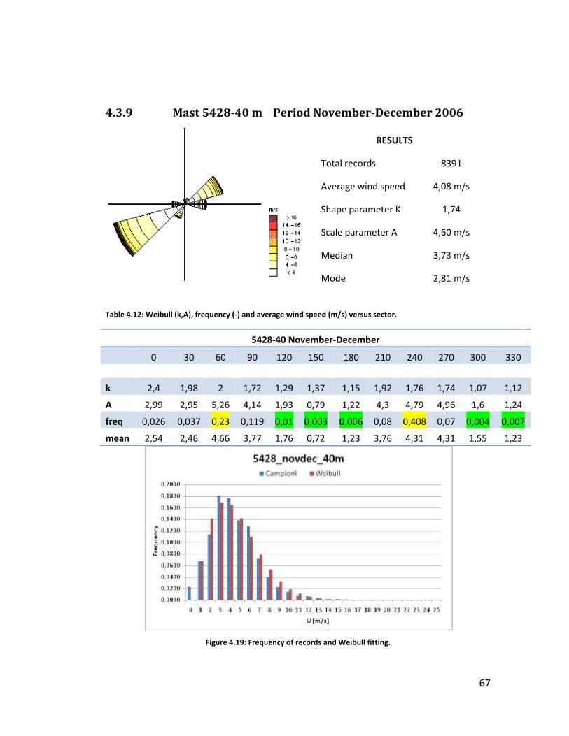
67
4.3.9 Mast 5428-40 m Period November-December 2006
Table 4.12: Weibull (k,A), frequency (-) and average wind speed (m/s) versus sector.
5428-40 November-December
0 30 60 90 120 150 180 210 240 270 300 330
k 2,4 1,98 2 1,72 1,29 1,37 1,15 1,92 1,76 1,74 1,07 1,12
A 2,99 2,95 5,26 4,14 1,93 0,79 1,22 4,3 4,79 4,96 1,6 1,24
freq 0,026 0,037 0,23 0,119 0,01 0,003 0,006 0,08 0,408 0,07 0,004 0,007
mean 2,54 2,46 4,66 3,77 1,76 0,72 1,23 3,76 4,31 4,31 1,55 1,23
Figure 4.19: Frequency of records and Weibull fitting.
RESULTS
Total records 8391
Average wind speed 4,08 m/s
Shape parameter K 1,74
Scale parameter A 4,60 m/s
Median 3,73 m/s
Mode 2,81 m/s

68
4.3.10 Mast 5428-30 m Period November-December 2006
4.13: Weibull (k,A), frequency (-) and average wind speed (m/s) versus sector.
5428-30 November-December
0 30 60 90 120 150 180 210 240 270 300 330
k 2,24 1,98 2,23 1,86 1,23 1,73 1,17 1,94 1,77 1,73 1,17 0,89
A 2,58 2,81 4,69 3,87 1,71 0,77 1,12 4,18 4,67 4,84 1,74 0,91
freq 0,026 0,037 0,23 0,119 0,01 0,003 0,006 0,08 0,408 0,07 0,004 0,007
mean 2,18 2,34 4,13 3,45 1,61 0,69 1,13 3,62 4,2 4,17 1,58 1,11
Figure 4.20: Frequency of records and Weibull fitting.
RESULTS
Total records 8391
Average wind speed 3,84 m/s
Shape parameter K 1,81
Scale parameter A 4,37 m/s
Median 3,57 m/s
Mode 2,80 m/s

69
4.4 Mean Speed per sector tables
4.4.1 Mast 5424
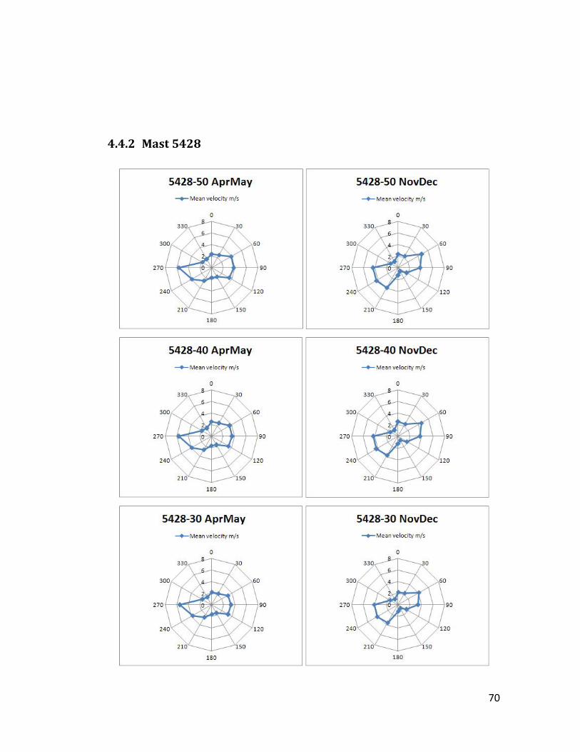
70
4.4.2 Mast 5428
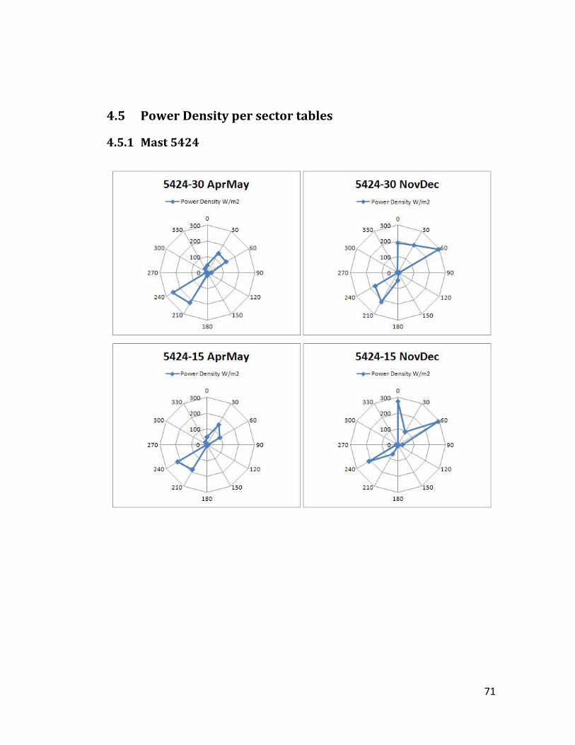
71
4.5 Power Density per sector tables
4.5.1 Mast 5424

72
4.5.2 Mast 5428

73
4.6 Remarks The terrain characteristics of the site and wind experimental data have been
presented.
The performed analysis allowed to highlight the dominant wind direction sectors,
corresponding to 30 and 210 degrees, for the tower 5424, while 60 and 240 degrees,
for the tower 5428.
The tower 5424 has shown a different behavior of the flow between the two
measurement station, respectively 15 and 30 meters, in the period November-
December. This fact can be related to some kind of thermal seasonal effects which
can influence the flow in a region very close to the ground. It must be noticed, in this
case, the position of the tower 5424 in proximity of a cliff, which can induce
orographic effects in the flow.
According to the selected dominant sectors, a preview of the position of the wind
turbines for a plant layout proposal can be done by considering to put them in a
series of rows perpendicular to the main wind directions.
The choice should be confirmed by the results of the simulations which will be carry
out in chapter 5 and 6.
74
CHAPTER 5. Test of the Free Stream Velocity (FSV)
5.1 Introduction The purpose of this chapter is to find the right settings in order to describe the
speed vertical profile of the flow given as a boundary condition. Particularly, the free
stream velocity of the geostrophic wind has been studied. In fact, the scalar value of
the free stream velocity can be set in WindSim by the user in the Windfield module.
The analysis of this input parameter has been done in three steps: first of all a
mesoscale model of the considered site has been created, keeping a coarse grid
resolution; then, as a second step, a smaller microscale model with medium grid
resolution has been studied, in order to put in evidence the recirculation effect of
the flow; finally, another microscale model with fine grid resolution has been built,
finding as a result the optimum value of the free stream velocity to set in WindSim
for further simulations.
The microscale models have been studied using the “nesting technique”: this
procedure consists in running a simulation of the windfield in the mesoscale model
and using this one to extract boundary conditions to be applied to the microscale
models, which have to be created therefore in a zone inside the mesoscale site.
5.2 Mesoscale Model The mesoscale model is presented in this section. The horizontal velocity field has
been calculated; using data of the tower 5428 at 50 meters height to scale the
results, the relative maps obtained with free stream velocities of 10 and 20 m/s are
respectively shown in Figure 5.1 and 5.2.
It must be noticed that in proximity of the tower position the maps show a value
equal to 1, demonstrating that the scale procedure is correct.
The maps have been extracted for 4 wind directions: 0, 90, 180, 270 degrees, at 30
and 50 meters height.
The test of the free stream velocity has been carried out for 4 scalar values: 1, 5, 10
and 20 m/s.

75
The general parameters set for the simulations are displayed in the following tables
5.1 and 5.2.
Geometrical model
Table 5.1: Input parameters of the geometrical model
INPUT PARAMETER VALUE Maximum number of cells 100000 Real number of cells 98532 X-resolution 210 m Y-resolution 210 m Number of cells in X-direction 67 Number of cells in Y-direction 60 Number of cells in Z-direction 20 Height distribution factor 0,1 Height of the model 4938 m First cell minimum height 44,8 m First cell maximum height 57,2 m
Numerical model
Table 5.2: Settings for the numerical model
BOUNDARY CONDITIONS Top wall with no friction Geostrophic height 500 m Free stream wind speed 1-5-10-20 m/s Wind direction 0-90-180-270 degrees Turbulence model standard k−ε
SOLVER SETTINGS Solver Coupled Number of iterations 50
Any important variation has been recognized, mostly in the zone of the plateau
containing the two mast measurements.
Anyhow, it can be seen that there is a directional sector, corresponding to 90
degrees, in which some small variations in the wind field are more evident. In this

76
case the wind is blowing from the east sector, from the plateau perpendicular to the
valley.
Figure 5.1: Speed-2D at 30 m height for sector 90 and velocity 10 m/s.
Figure 5.2: Speed-2D at 30 m height for sector 90 and velocity 20 m/s.
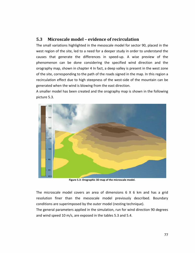
77
5.3 Microscale model – evidence of recirculation The small variations highlighted in the mesoscale model for sector 90, placed in the
west region of the site, led to a need for a deeper study in order to understand the
causes that generate the differences in speed-up. A wise preview of the
phenomenon can be done considering the specified wind direction and the
orography map, shown in chapter 4 In fact, a deep valley is present in the west zone
of the site, corresponding to the path of the roads signed in the map. In this region a
recirculation effect due to high steepness of the west-side of the mountain can be
generated when the wind is blowing from the east direction.
A smaller model has been created and the orography map is shown in the following
picture 5.3.
Figure 5.3: Orographic 3D map of the microscale model.
The microscale model covers an area of dimensions 6 X 6 km and has a grid
resolution finer than the mesoscale model previously described. Boundary
conditions are superimposed by the outer model (nesting technique).
The general parameters applied in the simulation, run for wind direction 90 degrees
and wind speed 10 m/s, are exposed in the tables 5.3 and 5.4.

78
Geometrical model
Table 5.3: Input parameters for geometrical model in the mesoscale model.
INPUT PARAMETER VALUE Maximum number of cells 500000 Real number of cells 499392 X-resolution 26 m Y-resolution 26 m Number of cells in X-direction 135 Number of cells in Y-direction 135 Number of cells in Z-direction 25 Height distribution factor 0,1 Height of the model 5000 m First cell minimum height 17,5 m First cell maximum height 22,2 m
Numerical model
Table 5.4: Settings for the numerical model.
BOUNDARY CONDITIONS Top Wall with no friction Geostrophic height From mesoscale model (500 m) Free stream wind speed From mesoscale model (10 m/s) Wind direction 90 degres (East) Turbulence model Standard k−ε
SOLVER SETTINGS Solver Coupled Number of iterations 500

79
Some vertical profiles have been extracted in the positions described in the picture
5.4 below to understand the behavior of the flow above the microscale refined
model.
Figure 5.4: Site of extraction of vertical profiles.
The analysis of the microscale model has shown the presence of a big recirculation
bubble, downstream of the mountain with wind direction of 90 degrees, extending
for 500 meters above ground level, as shown in pictures 5.5 and 5.6.
Figure 5.5: Vertical profiles in position 6.

The presence of the flow separation region can be connected to the variations in
speed-up maps recognized in the mesoscale model, the separated flow obtained for
the 90 degrees sector run is highlighted by means of streamlines colored by velocity
magnitude reported in the figure 5.7 .A more accurate analysis of the microscale
model has been also done, this will be presented in the next paragraph.
Figure 5.6: Vertical profiles in position
The presence of the flow separation region can be connected to the variations in
up maps recognized in the mesoscale model, the separated flow obtained for
the 90 degrees sector run is highlighted by means of streamlines colored by velocity
itude reported in the figure 5.7 .A more accurate analysis of the microscale
model has been also done, this will be presented in the next paragraph.
Figure 5.7: Particle tracing of the flow over the microscale model.
Figure 5.6: Vertical profiles in position 11.
The presence of the flow separation region can be connected to the variations in
up maps recognized in the mesoscale model, the separated flow obtained for
the 90 degrees sector run is highlighted by means of streamlines colored by velocity
itude reported in the figure 5.7 .A more accurate analysis of the microscale
model has been also done, this will be presented in the next paragraph.
Figure 5.7: Particle tracing of the flow over the microscale model.
10 m/s
80
The presence of the flow separation region can be connected to the variations in
up maps recognized in the mesoscale model, the separated flow obtained for
the 90 degrees sector run is highlighted by means of streamlines colored by velocity
itude reported in the figure 5.7 .A more accurate analysis of the microscale
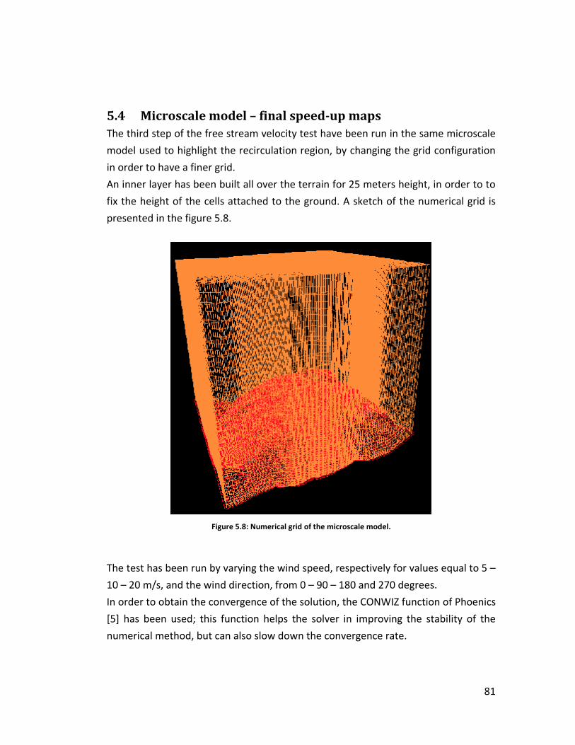
81
5.4 Microscale model – final speed-up maps The third step of the free stream velocity test have been run in the same microscale
model used to highlight the recirculation region, by changing the grid configuration
in order to have a finer grid.
An inner layer has been built all over the terrain for 25 meters height, in order to to
fix the height of the cells attached to the ground. A sketch of the numerical grid is
presented in the figure 5.8.
Figure 5.8: Numerical grid of the microscale model.
The test has been run by varying the wind speed, respectively for values equal to 5 –
10 – 20 m/s, and the wind direction, from 0 – 90 – 180 and 270 degrees.
In order to obtain the convergence of the solution, the CONWIZ function of Phoenics
[5] has been used; this function helps the solver in improving the stability of the
numerical method, but can also slow down the convergence rate.
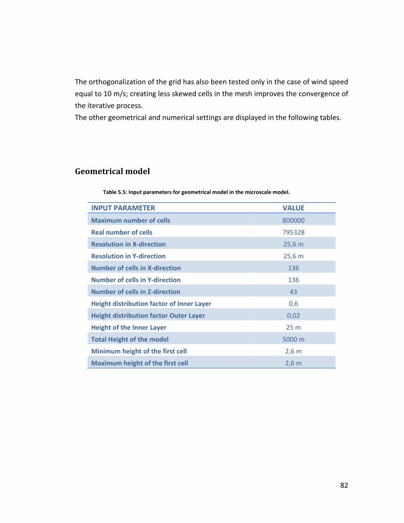
82
The orthogonalization of the grid has also been tested only in the case of wind speed
equal to 10 m/s; creating less skewed cells in the mesh improves the convergence of
the iterative process.
The other geometrical and numerical settings are displayed in the following tables.
Geometrical model
Table 5.5: Input parameters for geometrical model in the microscale model.
INPUT PARAMETER VALUE
Maximum number of cells 800000
Real number of cells 795328
Resolution in X-direction 25,6 m
Resolution in Y-direction 25,6 m
Number of cells in X-direction 136
Number of cells in Y-direction 136
Number of cells in Z-direction 43
Height distribution factor of Inner Layer 0,6
Height distribution factor Outer Layer 0,02
Height of the Inner Layer 25 m
Total Height of the model 5000 m
Minimum height of the first cell 2,6 m
Maximum height of the first cell 2,6 m

83
Numerical model
Tabella 5.6: Settings for the numerical model.
BOUNDARY CONDITIONS Top Wall with no friction Geostrophic height From linked model (500 m) Free stream wind speed From linked model (variable) Wind direction 0 - 90 – 180 – 270 Turbulence model standard k-ε
SOLVER SETTINGS Solver Coupled Number of iterations 500 – 800 – 400
The high number of cells built up in the microscale model required some time to
arrive to a good convergence level, which has been kept constant in all the
simulations. Anyhow, few critical runs have been found, mostly in the simulation for
10 m/s: in the speed-up maps some areas in which divergence is growing up are well
evident; this tendency to diverge has been reduced by increasing the free stream
velocity, therefore the tests with 20 m/s are the ones that showed less problems of
convergence. This fact let to think that in such a complex terrain and in such fine
grid resolution the default value of the free stream velocity is not good enough.
A presentation of this phenomenon can be seen in the figure 5.9, where in the left
zone of the picture is shown a critical area; the problems are mostly relevant when
wind is blowing from East sector, confirming the hypothesis by which the small
variation in speed-up maps can be strictly connected to flow separation effects.
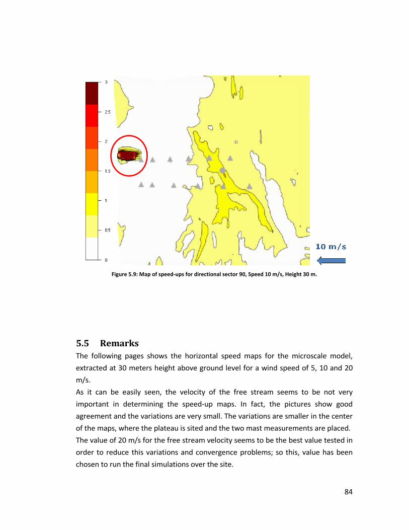
5.5 RemarksThe following pages shows the horizontal speed maps for the microscale model,
extracted at 30 meters height above ground level
m/s.
As it can be easily seen, the velocity of the free stream seems to be not very
important in determining the speed
agreement and the variations are very small. The variations are
of the maps, where the plateau is sited and the two mast measurements are placed.
The value of 20 m/s for the free stream velocity seems to be the best value tested
order to reduce this variations and convergence problems; so this
chosen to run the final simulations over the site.
Figure 5.9: Map of speed-ups for directional sector 90, Speed 10 m/s, Height 30 m.
Remarks The following pages shows the horizontal speed maps for the microscale model,
extracted at 30 meters height above ground level
As it can be easily seen, the velocity of the free stream seems to be not very
important in determining the speed-up maps. In fact, the pictures show good
agreement and the variations are very small. The variations are
of the maps, where the plateau is sited and the two mast measurements are placed.
he value of 20 m/s for the free stream velocity seems to be the best value tested
order to reduce this variations and convergence problems; so this
chosen to run the final simulations over the site.
ups for directional sector 90, Speed 10 m/s, Height 30 m.
The following pages shows the horizontal speed maps for the microscale model,
extracted at 30 meters height above ground level for a wind speed of 5, 10 and 20
As it can be easily seen, the velocity of the free stream seems to be not very
up maps. In fact, the pictures show good
agreement and the variations are very small. The variations are smaller in the center
of the maps, where the plateau is sited and the two mast measurements are placed.
he value of 20 m/s for the free stream velocity seems to be the best value tested
order to reduce this variations and convergence problems; so this, value has been
chosen to run the final simulations over the site.
84
The following pages shows the horizontal speed maps for the microscale model,
for a wind speed of 5, 10 and 20
As it can be easily seen, the velocity of the free stream seems to be not very
up maps. In fact, the pictures show good
smaller in the center
of the maps, where the plateau is sited and the two mast measurements are placed.
he value of 20 m/s for the free stream velocity seems to be the best value tested in
value has been

85
To improve the results of this test, some other studies can be done: first of all a
difference in speed-up value between various maps can be calculated, in order to
have a concrete value to read and understand; then, a further turbulence model like
the k-ε RNG can be tested and a different solver, the segregated solver.
Finally, also the diagonal wind directions should be tested, at least for the dominant
sectors of the experimental data shown in chapter 4.
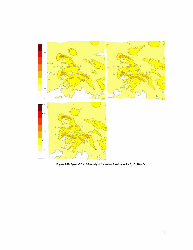
86
Figure 5.30: Speed-2D at 30 m height for sector 0 and velocity 5, 10, 20 m/s.
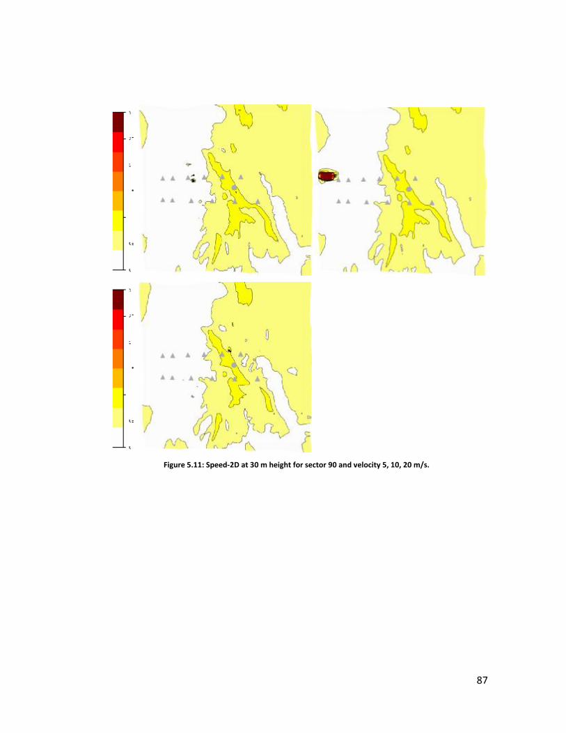
87
Figure 5.11: Speed-2D at 30 m height for sector 90 and velocity 5, 10, 20 m/s.

88
Figure 5.12: Speed-2D at 30 m height for sector 180 and velocity 5, 10, 20 m/s.

89
Figure 5.13: Speed-2D at 30 m height for sector 270 and velocity 5, 10, 20 m/s.
90
CHAPTER 6. Analysis of the wind field over the site.
6.1 Introduction
In this chapter a series of CFD simulations of the wind flow over a complex site in
central Italy has been carried out. Different boundary condition, corresponding to
different direction of the wind rose have been employed. The results of this CFD
analysis are used to perform a cross checking procedure of the experimental wind
data.
The geometrical model used in the simulations encloses the entire site and was
resolved with a grid able to guarantee accurate results, as shown in chapter 5.
The cross checking procedure has been conducted by using the transferred
climatology object, included in the WindSim software. As described in chapter 1,
when multiple measurement masts are available in one site, it is possible to predict
the wind resources in one measurement station using data available in the other
measurement station. The comparison between experimental and CFD data can be
done by producing graphs and calculating RMS errors to evaluate the accuracy of
the results. Velocity vertical profiles and turbulence intensity vertical profiles have
been also calculated and analyzed.
6.2 Geometrical model The geometrical domain is based on a unique model to solve the Wind Field. A
refinement of the major interest zone has been created, containing the plateau
where the two measurement masts are located.
The characteristics of the geometrical model are shown in the table 6.1.
91
Table 6.1: Geometrical model characteristics.
Geometrical model Total number of cells 3136000 Extension Km 14,2 x 14,2 x_resolution min 134 m – max 30 m y_resolution min 134 m – max 30 m Number of cells in x direction 280 Number of cells in y direction 280 Number of cells in z direction 40 Height Distibution Factor 0,01 Height of the model 5000 m Minimum height of the first cell 2,4 m Maximum height of the first cell 3,2 m Number of cells in first 100 m height 6
6.3 Numerical Model The 3D Wind Field of the site has been calculated through the WindSim software.
This program is a powerful tool which solves the Reynolds Averaged Navier Stokes
(RANS) equations for turbulent flows. The numerical model contains the continuity
equation and the three momentum equations. The energy equation has not been
solved since thermal effects have not been considered in the simulations. The
closure problem of turbulent flows has been solved by introducing the standard κ−ε
turbulence model. The boundary conditions and the settings for the solver are listed
in table 6.2

92
Table 6.2: Boundary conditions and solver settings
Boundary conditions Top wall with no friction Geostrophic height 500 m Free stream wind speed 20 m/s Wind directions 12 sectors
Turbulence closure Turbulence model standard k-ε YAP correction enabled
Solver settings Solver type Segregated Number of iteration 600 Convergence Wizard enabled
6.4 Simulations The total time needed to carry out the simulations was about 12 full days, one day
per sector. The computer used for the simulations was a Dell Precision T5400,
equipped by a quad-core CPU Intel Xeon with frequency 2,33 GHz each and 8 GBytes
of RAM.
The residual values showing the obtained convergence level are shown in figure 6.1,
for the simulations corresponding to the different directional sectors. A correct
convergence level has been obtained in each sector.
Figure 6.1 a/b/c: Residual values for sectors 0, 30 and 60 degrees.
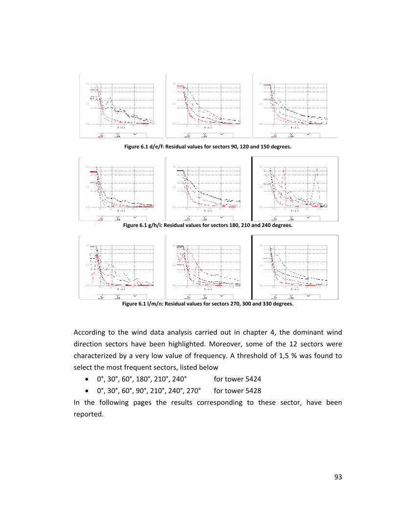
93
Figure 6.1 d/e/f: Residual values for sectors 90, 120 and 150 degrees.
Figure 6.1 g/h/i: Residual values for sectors 180, 210 and 240 degrees.
Figure 6.1 l/m/n: Residual values for sectors 270, 300 and 330 degrees.
According to the wind data analysis carried out in chapter 4, the dominant wind
direction sectors have been highlighted. Moreover, some of the 12 sectors were
characterized by a very low value of frequency. A threshold of 1,5 % was found to
select the most frequent sectors, listed below
• 0°, 30°, 60°, 180°, 210°, 240° for tower 5424
• 0°, 30°, 60°, 90°, 210°, 240°, 270° for tower 5428
In the following pages the results corresponding to these sector, have been
reported.

94
6.5 Vertical profiles of Velocity
Tower 5424 (CLIFF) The sector chosen after analysis by frequency distribution of the tower 5424, placed
near the cliff, are 0°, 30°, 60°, 180°, 210°, 240° and the vertical profiles of mean wind
velocity relative to this sector are reported.
Figure 6.2 a/b/c/d/e/f: Velocity vertical profiles for tower 5424.
The values of the velocity U30 (experimental wind velocity at 30 meters height) have
been used to calculate data in a non dimensional form, in order to make a
comparison with CFD vertical profiles, also scaled with the corresponding velocity
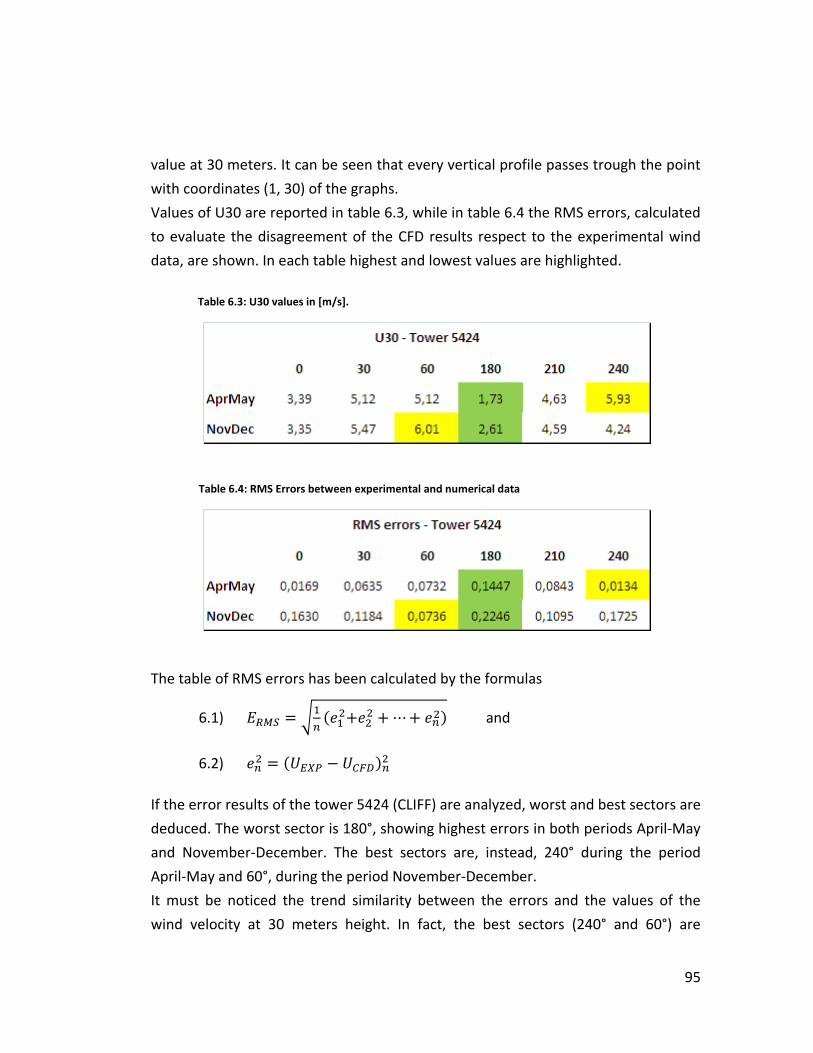
95
value at 30 meters. It can be seen that every vertical profile passes trough the point
with coordinates (1, 30) of the graphs.
Values of U30 are reported in table 6.3, while in table 6.4 the RMS errors, calculated
to evaluate the disagreement of the CFD results respect to the experimental wind
data, are shown. In each table highest and lowest values are highlighted.
Table 6.3: U30 values in [m/s].
Table 6.4: RMS Errors between experimental and numerical data
The table of RMS errors has been calculated by the formulas
6.1) = ( + +⋯+ ) and
6.2) = ( − )
If the error results of the tower 5424 (CLIFF) are analyzed, worst and best sectors are
deduced. The worst sector is 180°, showing highest errors in both periods April-May
and November-December. The best sectors are, instead, 240° during the period
April-May and 60°, during the period November-December.
It must be noticed the trend similarity between the errors and the values of the
wind velocity at 30 meters height. In fact, the best sectors (240° and 60°) are
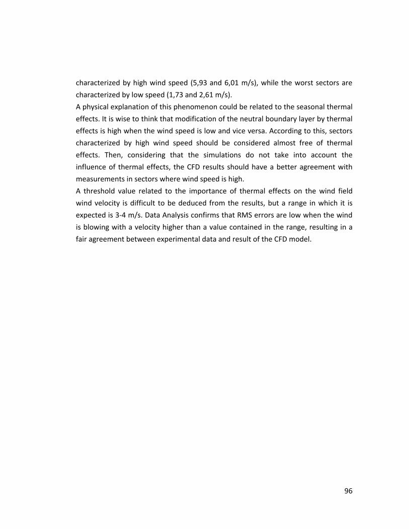
96
characterized by high wind speed (5,93 and 6,01 m/s), while the worst sectors are
characterized by low speed (1,73 and 2,61 m/s).
A physical explanation of this phenomenon could be related to the seasonal thermal
effects. It is wise to think that modification of the neutral boundary layer by thermal
effects is high when the wind speed is low and vice versa. According to this, sectors
characterized by high wind speed should be considered almost free of thermal
effects. Then, considering that the simulations do not take into account the
influence of thermal effects, the CFD results should have a better agreement with
measurements in sectors where wind speed is high.
A threshold value related to the importance of thermal effects on the wind field
wind velocity is difficult to be deduced from the results, but a range in which it is
expected is 3-4 m/s. Data Analysis confirms that RMS errors are low when the wind
is blowing with a velocity higher than a value contained in the range, resulting in a
fair agreement between experimental data and result of the CFD model.
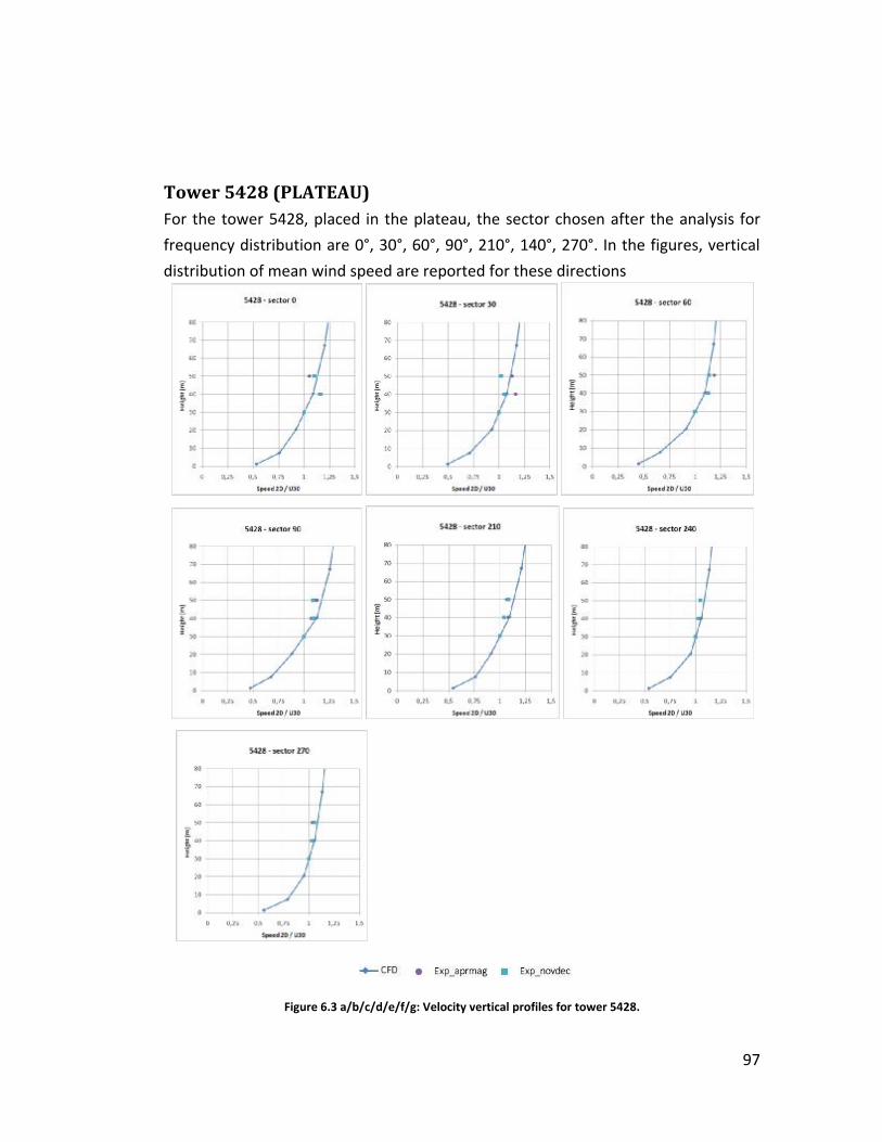
97
Tower 5428 (PLATEAU) For the tower 5428, placed in the plateau, the sector chosen after the analysis for
frequency distribution are 0°, 30°, 60°, 90°, 210°, 140°, 270°. In the figures, vertical
distribution of mean wind speed are reported for these directions
Figure 6.3 a/b/c/d/e/f/g: Velocity vertical profiles for tower 5428.
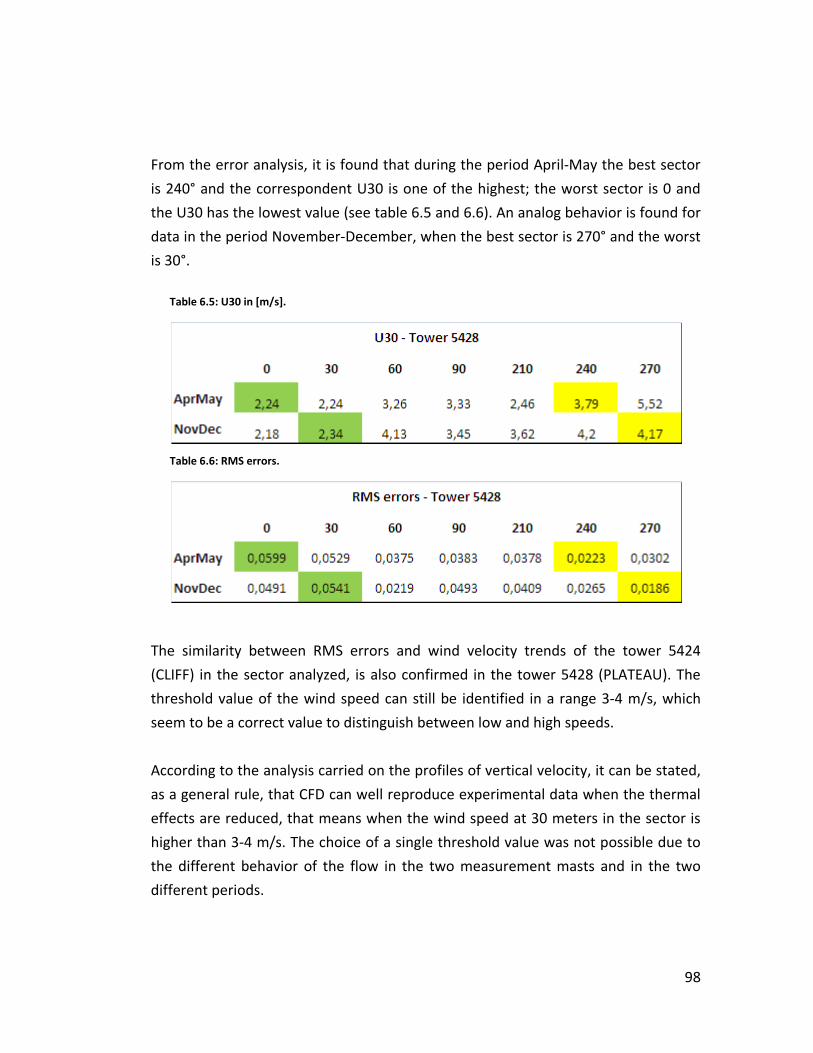
98
From the error analysis, it is found that during the period April-May the best sector
is 240° and the correspondent U30 is one of the highest; the worst sector is 0 and
the U30 has the lowest value (see table 6.5 and 6.6). An analog behavior is found for
data in the period November-December, when the best sector is 270° and the worst
is 30°.
Table 6.5: U30 in [m/s].
Table 6.6: RMS errors.
The similarity between RMS errors and wind velocity trends of the tower 5424
(CLIFF) in the sector analyzed, is also confirmed in the tower 5428 (PLATEAU). The
threshold value of the wind speed can still be identified in a range 3-4 m/s, which
seem to be a correct value to distinguish between low and high speeds.
According to the analysis carried on the profiles of vertical velocity, it can be stated,
as a general rule, that CFD can well reproduce experimental data when the thermal
effects are reduced, that means when the wind speed at 30 meters in the sector is
higher than 3-4 m/s. The choice of a single threshold value was not possible due to
the different behavior of the flow in the two measurement masts and in the two
different periods.

99
The characteristics of the relation between wind speed U30 and RMS errors on
mean wind speed are summarized in figure 6.4. It can be stated that errors
calculated for tower 5428 are lower than those calculated for tower 5424. The fact
could be related to the height of the three measurement stations of the tower 5428
(30-40-50 m) respect to the stations of tower 5424 (15-30m). Measurements close
to the ground are difficult to predict due to the complex orographic effects.
Figure 6.4: Relation between RMS errors and sector wind speed.
Moreover, a general trend for RMS errors can be underlined in the graph, showing
that errors become lower when wind speed U30 is becoming higher. Again, this fact
is related to the importance of thermal effects, that decreases in presence of a high
wind speed.

100
Anyhow, the trend of the linear interpolation is different according to the
measurement period. Thermal effects are different along the year, due to solar
radiation and thermal inertia of the terrain, inducing different wind breezes in the all
area.
Finally, it must be noticed that in the tower 5424 for the period November-
December there is the best alignment of the data, while in the period April-May the
marker circled in black shows a non correct behavior compared with the other data
and should be excluded by the analysis. The point corresponds to sector 0°, which
has a low frequency during the considered measurement period and could be
influenced by errors in the statistic analysis. Concerning the tower 5428, data are
well disposed in a trend in both periods.
101
6.6 Turbulence Intensity Vertical Profiles
In this paragraph vertical profiles of turbulence intensity (T.I.) are reported and
analyzed. The figures 6.5 and 6.6 show the comparison between the measured
turbulence intensity values and the results of CFD simulation.
The experimental T.I. values have been calculated by the time-history of wind data
as a ratio between the standard deviation of wind velocity and the mean wind
velocity evaluated for the instantaneous measurements taken in 10 minutes
6.3.3) . . =
where
σ is the standard deviation of wind velocity [m/s] U is the mean velocity [m/s]
By organizing experimental data for wind direction it is possible to group these
angles in sectors (in the specific case one sector every 30° for a total of 12 sectors)
and to consider the wind velocity and the associated T.I. value. Then, it is possible to
create twelve scatter graph, where T.I. is a function of U. In general, these graphs
show a cloud of points that can be approximate by an hyperbolic function. Data
reaching an infinite value of T.I. for low wind velocity are present while the expected
trend goes toward zero when wind velocity grows. The common practice eliminates
the high values of turbulent intensity associated to low wind speed, that are
probably affected by thermal effects, when an interpolation of the cloud of points is
required. According to this practice rule the TI was evaluated rejecting the values
connected to low mean wind velocity. The threshold value was chosen following the
conclusions of the previous paragraph 6.5, where a threshold range was indicated in
U30 = 3÷4 m/s. In these particular analysis the value of U=4 m/s has been used to
filter experimental data.
The CFD simulations did not take into account thermal effects, thereafter under
estimating the turbulence intensity data. A procedure of rejecting these data is then
needed to reduce the thermal effects in the experimental data used for comparison.
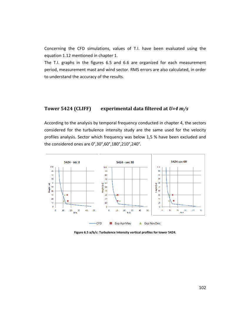
102
Concerning the CFD simulations, values of T.I. have been evaluated using the
equation 1.12 mentioned in chapter 1.
The T.I. graphs in the figures 6.5 and 6.6 are organized for each measurement
period, measurement mast and wind sector. RMS errors are also calculated, in order
to understand the accuracy of the results.
Tower 5424 (CLIFF) experimental data filtered at U=4 m/s
According to the analysis by temporal frequency conducted in chapter 4, the sectors
considered for the turbulence intensity study are the same used for the velocity
profiles analysis. Sector which frequency was below 1,5 % have been excluded and
the considered ones are 0°,30°,60°,180°,210°,240°.
Figure 6.5 a/b/c: Turbulence Intensity vertical profiles for tower 5424.

103
Figure 6.5 d/e/f: Turbulence Intensity vertical profiles for tower 5424.
By general overview of the turbulence intensity vertical profiles it seems that CFD
well approximates the experimental data. In tables 6.7 and 6.8, RMS errors related
to vertical profiles have been calculated and presented together with the U30 wind
velocity.
Table 6.7: RMS errors for tower 5424.
Table 6.8: Values of U30 for tower 5424.

104
Analyzing RMS error table for tower 5424, it is found that the sectors where
turbulence intensity level is higher is 240°, during both periods April-May and
November-December. Sectors where turbulence intensity is lower are sector 180°
and 60°, respectively for periods April-May and November-December. By
considering the RMS table and the U30 table, different behaviors for the two
periods of reference can be found. In fact, during April-May the error seems to
increase with the wind speed, while during November –December the error seems
to decrease when U30 is growing. This behavior is well represented by the trend
lines shown in figure 6.7.
In general, it can be stated that the values of the T.I. seem to be strongly linked to
the seasonal thermal effects. As was already said before, the solar radiation and the
thermal inertia of the terrain can generate different wind breezes in the
measurement periods, also influencing the turbulence level. A stronger influence on
the turbulence intensity level can be due also to the orographic effects. The tower
5424 is placed in a cliff, where vertical component of velocity are present and can be
strongly variable in intensity during the whole year because of the different solar
radiation. Particularly, strong solar radiation near a cliff can generate a intense
vertical wind, where the fluctuations are stronger. This phenomenon could explain
the trend relative to April-May period in figure 6.7, where in general the errors
increase with the U30.
Finally, it must be said that turbulence is a parameter very difficult to measure,
especially in atmospheric flows, and that a only a longer measurement campaign
can guarantee more accurate results. Due to all this consideration, the agreement
between experimental data and CFD results for mast 5424 was fairly good.

105
Tower 5428 (PLATEAU) experimental data filtered at u=4 m/s
Figure 6.6 a/b/c/d/e/f/g: Turbulence Intensity vertical profiles for tower 5428.
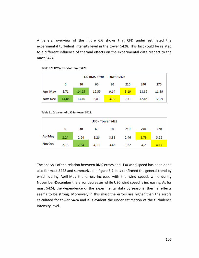
106
A general overview of the figure 6.6 shows that CFD under estimated the
experimental turbulent intensity level in the tower 5428. This fact could be related
to a different influence of thermal effects on the experimental data respect to the
mast 5424.
Table 6.9: RMS errors for tower 5428.
Table 6.10: Values of U30 for tower 5428.
The analysis of the relation between RMS errors and U30 wind speed has been done
also for mast 5428 and summarized in figure 6.7. It is confirmed the general trend by
which during April-May the errors increase with the wind speed, while during
November-December the error decreases while U30 wind speed is increasing. As for
mast 5424, the dependence of the experimental data by seasonal thermal effects
seems to be strong. Moreover, in this mast the errors are higher than the errors
calculated for tower 5424 and it is evident the under estimation of the turbulence
intensity level.
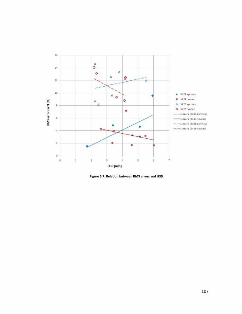
107
Figure 6.7: Relation between RMS errors and U30.

108
6.7 Cross Checking of wind data
In the following paragraphs the cross checking of the experimental data, as
explained in chapter 1, is presented. The WindSim feature, called transferred
climatology object, was used. As previously described when multiple measurement
masts are available in one site, it is possible to predict by CFD calculation the wind
resources in one measurement station using data available in the other
measurement station. In other words, it’s possible to transfer wind data from the
original position to the other taking into account the different orographic and
roughness effects
The cross checking has been studied using two different procedures, using as scaling
variable the mean wind velocity per sector and the speed-up values, respectively.
In the first case the experimental mean velocity values have been extracted by the
time history, while all the CFD values have been calculated using the sector
interpolation function [4] of WindSim.
In the second case, relative to the speed-up calculation, two methods have been
used, one considering the sector interpolation and the other one without this
option. Concerning the experimental speed-up, this value was calculated directly
from experimental dataset, by a ratio between the mean velocity in the reference
mast and the mean velocity in the new position.
Sector interpolation
The sector interpolation function is a correction function of WindSim, needed when
the CFD results must be weighted against one experimental data-set, in order to
determine the horizontal wind speed map.
When the wind direction boundary condition is given, it is applied at the boundaries
of the model, by describing a geostrophic wind. Nevertheless the wind evaluated in
the internal zone can be deviated by orographic effects, especially close to the
ground. For instance, if two simulations are run for sectors 0° and 30° as boundary
conditions, in the center of the domain the wind direction could be, for instance, 2°
and 35° respectively. In this case there will be a mismatch between the directions of

109
the wind rose and the directions of the CFD results. To solve this problems, the
sector interpolation function is helpful, in order to modify the CFD results.
The wind directions found with the CFD must be referred at one direction of the
wind rose and this is done by a linear interpolation procedure. For instance, the
correct CFD velocity for the direction 30° is obtained weighting the two velocities
calculated (2° and 35°) in which the 30° direction is comprised. The weight is
proportional to the distance of the actual CFD velocity from the wind rose direction.
Once this weighted average of sector 0 and 30 is done, the obtained dataset is used
to scale the experimental climatology data for sector 30, allowing the preparation of
the wind resources map. This procedure is repeated for all the directional sectors at
the climatology.
6.7.1 Mean wind velocity The concept of the accuracy of the CFD calculation ha also been applied in the cross
checking procedure, and all the sector with a temporal frequency below 1,5 % have
been excluded. Moreover, the conclusions valid for velocity vertical profiles have
been also applied to the cross checking and the sectors in which the thermal effects
are strongly reduced have been highlighted with a red circle, i.e. the sectors for
which U30 is included in or greater than the range 3 ÷ 4 m/s.
In figures 6.8 the results of the cross-checking procedure by mean wind velocity are
presented. For instance in figure 6.8a, for each direction sector, the velocity on mast
5424 in the period April-May, forecasted by data on mast 5428 at different height,
are reported.

110
Figure 6.8 a/b
Figure 6.8 c/d
Figure 6.8 e/f

111
Figure 6.8 g/h
Figure 6.8 i/l
The graphs show a fair agreement between experiments and CFD in the sector
where seasonal thermal effects are reduced, i.e. in sectors marked with red circles in
the figures 6.8. Some disagreement is found in the period Nov-Dec at 15 m. In the
other sectors the errors generally increase, showing again the influence of the mean
velocity on the errors. The RMS errors, shown in table 6.8, have been calculated
taking into account only the sectors in which the thermal independence is obtained,
in order to establish which set of data can reproduce better the experimental data.
The table should be read in this way: on the left vertical column, the mast and
height for which experimental data are used as reference values in the cross
checking are listed. On the horizontal row, the mast and height were the wind data
are forecasted is arranged. Obviously, from 5428 mast only data on the 5424 mast
can be deduced, and vice versa.

112
Table 6.11: RMS error for cross checking by mean wind velocity.
According to the table 6.11 the best match is found in the period April-May, starting
from data of the station 5424 at 15 meters height and predicting the wind
characteristics in station 5428 at 30 meters height, situation that corresponds to the
graph 6.8 e.
Table 6.11 allows also to understand which dataset is to be used for a prediction of
the wind in the other tower. The best dataset corresponds to station 5424 at 15
meters high, as shown by the total RMS error. Considering that the 5424 tower is
positioned near a cliff this result could seem somehow peculiar. An explanation of
this phenomenon can be related to the fact that is relatively straightforward to
predict the flow at higher quotes and for non complex orography (mast 5428), even
starting from data at low quotes and placed in critical positions as a cliff (tower
5424).
In general, from table 6.11 it can be seen that errors are lower in the period April-
May and this could be explained by assuming that seasonal thermal effects are more
influent when the terrain is cooling (Nov-Dec) instead of warming up (Apr-May).

113
6.7.2 Speed-up In the figures 6.9 and 6.10 the results of the cross-checking by speed-up are
reported; the label “transf clima” refers to the simulation with the sector
interpolation option enabled, while the label “wecs” refers to the case with this
option switched off. The green triangular marker is related to the experimental
speed-up, calculated as the ratio between the two specified measurement stations.
For instance in figure 6.9a, for each direction sector, the velocity on mast 5424 at 15
meters in is forecasted by data on mast 5428 at 30 meters. The CFD calculations
with sector interpolation and without this options are compared with the
experimental speed-up.
The RMS errors are calculated only for sectors where thermal effects are reduced,
marked with the red circles.
Period April-May 2007
Figure 6.9 a/b
Figure 6.9 c/d

114
Figure 6.9 e/f
Figure 6.9 g/h
Figure 6.9 i/l
Figure 6.9 m/n
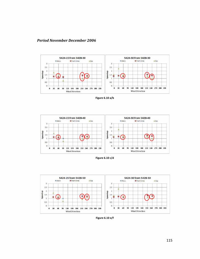
115
Period November December 2006
Figure 6.10 a/b
Figure 6.10 c/d
Figure 6.10 e/f

116
Figure 6.10 g/h
Figure 6.10 i/l
Figure 6.10 m/n

117
Tables 6.12 and 6.13 summarize the calculation of the RMS errors relative to the
cross-checking procedure conducted by speed-up and reported in the figures 6.9
and 6.10.
Table 6.12: RMS errors for period April-May.
Table 6.13: RMS errors for period November-December.
The results of the cross checking by speed-up instead of mean wind velocity
confirmed the results of the previous analysis. The period April-May was still better
reproduced by CFD calculations and the best dataset was the one at station 5424 at
15 meters height. Moreover, the sector interpolation option was found to be helpful

118
to have a better agreement during the period April-May, while in the period
November-December CFD results show worst match against experimental data.
It must be noticed also that the sector interpolation function does not influence in a
strong way the total error (shown in tables 6.12 and 6.13), which keeps the same
order of magnitude both in cases April-May and November-December.
6.8 Remarks
A CFD simulation of the windfield of a site in central Italy was carried out. The
chosen parameters to build the geometrical grid and to set the solver settings were
chosen to reach a sufficient accuracy level without any divergence problem.
The velocity vertical profiles were studied and the agreement between CFD and
experimental data was correct only in the dominant sectors where thermal effects
were reduced.
Turbulence intensity was also studied, showing that the WindSim code
underestimates the experimental data and that turbulence intensity level is strongly
influenced by seasonal thermal effects.
The cross checking of the experimental data collected by the two masts
measurement was finally performed. The best wind dataset in predicting wind
experimental data was found in station 5424 at 15 meters height,
The “sector interpolation” option [4] was tested, demonstrating that it can be
helpful in some case to find a better agreement between experimental and CFD
data.

119
CHAPTER 7. Proposal for a plant layout.
7.1 Introduction In the present chapter a proposal for a wind farm layout has been presented.
To do this, a wind resources map has been calculated by weighting the CFD results
against the chosen experimental climatology, precisely station 5428 at 50 meters
height.
According to literature [9], it is better to measure data at a vertical high distance
from the ground in a zone not influenced by orographic effects. In this case the
chosen station has all the required characteristics.
A wind park with 16 turbines was studied and the Annual Energy Production (AEP)
yield was finally calculated
7.2 Dataset April-May 5428-50 The wind rose of the climatology 5428-50 during the period April-May is reported in
figure 7.1, with the main parameters of the Weibull analysis.
Figure 7.1: Climatology 5428-50 Apr-May
In the graph reported in figure 7.2 the Weibull fitting of the experimental data is
presented, showing good agreement.
RESULTS
Total records 8784
Average wind speed 3,95 m/s
Shape parameter K 1,78
Scale parameter A 4,52 m/s
Median 3,68 m/s
Mode 2,84 m/s
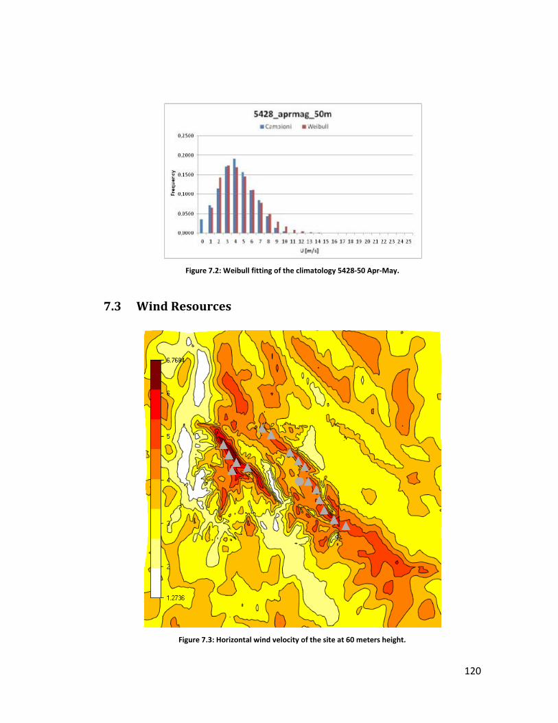
120
Figure 7.2: Weibull fitting of the climatology 5428-50 Apr-May.
7.3 Wind Resources
Figure 7.3: Horizontal wind velocity of the site at 60 meters height.

121
The figure 7.3 shows the horizontal wind velocity extracted in the site at 6 meters
height.
As it can be seen the higher speed values are located in the zone of the mountains,
surrounding the plateau where the stations were placed.
According to this consideration and the conclusions of the chapter 4, finding sectors
60 and 240 as dominant wind directions, 16 turbines have been placed in two rows
perpendicular to the dominant wind directions.
The position of the turbines can be seen by the figure 7.4, while a perspective view
of the wind park has been also presented in the figure 7.5.
Figure 7.4: Orography map with wind turbines position.

122
Figure 7.5: Perspective view of the wind park from West direction.
7.4 Annual Energy Production AEP The turbine chosen to calculate the AEP is the Gamesa G80 with 2000 kW of
nominal power output. Its characteristics are summarized in table 7.1.
Table 7.1: Characteristics of the turbine Gamesa G80
Model G80
Power 2000 kW
Rotor diameter 80 m
Number of blades 3
Lenght of the blades 39 m
Weight of each blade 6500 kg
Material of construction for blades Glass fiber reinforced with epoxy resin
Cut in velocity 4 m/s
Cut off velocity 25 m/s
Hub height 60 m
Control system
The generator is a doubly fed machine (DFM), whose speed and power is controlled through IGBT converters and PWM control

123
A picture of the turbine is presented in figure 7.6.
Figure 7.6: Turbine Gamesa G80 – 2000 kW
Other technical data of the turbine are shown in figure 7.7, reporting the power
curve.
Figure 7.7: Power curve of the turbine Gamesa G80 -2000 kW.
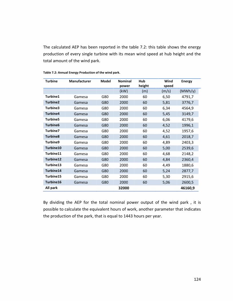
124
The calculated AEP has been reported in the table 7.2: this table shows the energy
production of every single turbine with its mean wind speed at hub height and the
total amount of the wind park.
Table 7.2: Annual Energy Production of the wind park.
Turbine Manufacturer Model Nominal power
Hub height
Wind speed
Energy
(kW) (m) (m/s) (MWh/y) Turbine1 Gamesa G80 2000 60 6,50 4791,7 Turbine2 Gamesa G80 2000 60 5,81 3776,7 Turbine3 Gamesa G80 2000 60 6,34 4564,9 Turbine4 Gamesa G80 2000 60 5,45 3149,7 Turbine5 Gamesa G80 2000 60 6,06 4179,6 Turbine6 Gamesa G80 2000 60 4,52 1996,1 Turbine7 Gamesa G80 2000 60 4,52 1957,6 Turbine8 Gamesa G80 2000 60 4,61 2018,7 Turbine9 Gamesa G80 2000 60 4,89 2403,3 Turbine10 Gamesa G80 2000 60 5,00 2539,6 Turbine11 Gamesa G80 2000 60 4,68 2148,2 Turbine12 Gamesa G80 2000 60 4,84 2360,4 Turbine13 Gamesa G80 2000 60 4,49 1880,6 Turbine14 Gamesa G80 2000 60 5,24 2877,7 Turbine15 Gamesa G80 2000 60 5,30 2915,6 Turbine16 Gamesa G80 2000 60 5,06 2600,5 All park 32000 46160,9
By dividing the AEP for the total nominal power output of the wind park , it is
possible to calculate the equivalent hours of work, another parameter that indicates
the production of the park, that is equal to 1443 hours per year.

125
7.5 Remarks The AEP of a wind farm constituted by 16 turbines has been calculated. The position
of the turbines was chosen considering the main wind direction sectors and the
wind resource map, obtained by weighting the CFD results against the climatology
5428 (plateau) at 50 meters height in the period Apr-May.
The total energy production of the park was 46,2 GWh per year, corresponding to
1443 hours of work at nominal power output.
For further analysis it could be interesting to have a complete one year wind data
set and to have wind data filtered with cases of atmospheric stability, in order to
avoid strong thermal effects which WindSim was not able to reproduce.
126
Conclusions
In this thesis the evaluation of wind energy resources over a site in central Italy was
conducted by means of the CFD code WindSim.
A series of 2D simulations were performed in order to validate the code. The code
validation process brought to find the correct discretization parameter capable to
guarantee grid-independent results. The “wall with no friction” boundary condition,
to be applied at the top of the geometrical model was chosen, in order to describe a
neutral stratified ABL. The comparison of the CFD results with numerical and
experimental results found in literature showed a fair agreement.
The second part of the study concerned the evaluation of the wind resources o a site
in Central Italy. The experimental wind data of two measurement masts (with
multiple measurement stations) were reduced and statistically analyzed.
Taking advantage of the validation phase results, 3D simulations were carried out for
a geometrical model reproducing the complex orography of the site. Firstly, a
correct value of the free stream velocity of the geostrophic wind was found, to avoid
convergence problems. A “nesting technique” in a coarse grid model was used to
reduce the computational resources.
Finally the simulations over a 14x14 km extended model with fine grid resolution
have been performed and the wind field over the whole site was calculated.
The results of the CFD calculations have been processed, in order to establish a
comparison between experimental data and calculated values. The Vertical profiles
of velocity and of turbulence intensity allowed the evaluation of RMS errors against
the experimental data. RMS errors of velocity profiles exhibit a direct relation with
the mean velocity of the directional sector, hereby showing a strong dependence on
thermal effects. Indeed, these effects are not taken into account by the CFD
simulations, whose numerical model is addressed to reproduce a neutral ABL. The
analysis of results on the wind rose sectors allowed to find a range of mean velocity
(3÷4 m/s) that discriminate whether or not data are influenced by thermal effects.
For high mean velocity a fair agreement was evident.

127
A cross-checking procedure of wind data was also performed. Using each mast as a
reference, the best agreement was found again for sectors where mean velocity is
high and thermal effects where negligible. The discrepancy between CFD results and
experimental data is acceptable because accurate ABL measurement are difficult to
obtain. Furthermore, this kind of analysis is normally addressed to evaluate the
correct wind resources distribution, instead of finding the true velocity field over the
site.
For the site under study, a wind resources map at 60 meters height has been
predicted and a proposal for a plant layout has been advanced, taking into account
the dominant direction sectors and the higher horizontal speed areas.
As a conclusion, the methodology presented in this thesis is relatively
straightforward and suitable for wind resources analysis. Nevertheless, the correct
setting of the CFD model and long term wind measurement are needed to
guarantee the correct accuracy. Fairly accurate results with neutral ABL simulations
are obtained only for directional sectors where negligible thermal effects are found.
This work demonstrates that the procedure is suitable for sites with complex
orography, in this showing advantages over linear methods normally for siting
evaluation.
128
Bibliography
[1] CRASTO G. – Numerical simulations of the Atmospheric Boundary Layer – PhD
thesis, Università degli Studi di Cagliari, February 2007
[2] YAMAGUTCHI, ISHIHARA, FUJINO, - Applicability of linear and non linear wind
prediction models to wind flow in complex terrain - Department of Civil Engineering,
University of Tokyo, Japan (2002)
[3] H. G. KIM, C. M. LEE & others – An experimental and numerical study of the
flow over two-dimensional hills – Journal of Wind Engineering and Industrial
Aerodynamics 66 (1997) 17-33
[4] WindSim module description – WindSim version 4.7.0 (2007)
[5] Phoenics online Encyclopedia – www.cham.co.uk (2008)
[6] WHITE, FRANK M. – Fluid mechanics IV edition – Mc Graw Hill International
Editions (1999)
[7] LARS DAVIDSON – An introduction to turbulence models – publication 97/2 –
November 2003 - Chalmers University of Technology, Goteborg, Sweden
[8] Technical specifications for wind measurement instruments -
www.nrgsystems.com/store (2008)
[9] ERICH HAU – Windturbines Fundamentals, Technologies, Application and
Economics –Springer (2000)
129
[10] JOHN F. WENDT – The differential equations of fluid dynamics, a review –
course note 121, September 1986 – Von Karman Institute for fluid dynamics, Rhode
Saint Genese Belgium
[11] G. DEGREZ – Introduction to CFD - course note 153, October 1998 – Von
Karman Institute for fluid dynamics, Rhode Saint Genese Belgium
[12] KAIMAL J.C., FINNIGAN J.J. – Atmospheric boundary layer flows: their structure
and measurement – Oxford University Press, New York, NY
[13] www.cfd-online.com (2008)
[14] GRAVDAHL A.R. - On the Sensitivity of Numerical Wind Field Modeling -
WINDPOWER, Los Angeles (2007)
[15] MORENOP., GRAVDAHL A.R., ROMERO M. - Wind Flow over Complex Terrain:
Application of Linear and CFD Models - European Wind Energy Conference and
Exhibition, Madrid, 2003.