UNIVERSIDAD POLITÉCNICA

DE MADRID

ESCUELA TÉCNICA SUPERIOR DE INGENIEROS

INFORMÁTICOS

EIT DIGITAL MASTER IN DATA SCIENCE

Maggy: Open-Source AsynchronousDistributed Hyperparameter Optimization

Based on Apache Spark

Master Thesis

Moritz Johannes Meister

Madrid, July 2019

This thesis is submitted to the ETSI Informáticos at Universidad Politécnica de Madrid in

partial fulfillment of the requirements for the degree of EIT Digital Master in Data Science.

Master ThesisEIT Digital Master in Data ScienceThesis Title: Maggy: Open-Source Asynchronous Distributed Hyperparameter Optimiza-

tion Based on Apache Spark

July 2019

Author: Moritz Johannes Meister

Bachelor of Science

Maastricht University

Supervisor: Co-supervisor:Alberto Mozo Jim Downling

Professor Associate Professor

SISTEMAS INFORMÁTICOSDivision of Software

and Computer Systems

E.T.S DE ING. DE

SISTEMAS INFORMÁTICOSKTH ICT School

Universidad Politécnica de MadridKTH Royal Institute of Technology

in Stockholm

ETSI Informáticos

Universidad Politécnica de Madrid

Campus de Montegancedo, s/n

28660 Boadilla del Monte (Madrid)

Spain

Abstract

Title of the thesis: Maggy: Open-Source Asynchronous Distributed Hyperparameter Op-

timization Based on Apache Spark

Author: Moritz Johannes Meister

Advisors: Kim Hammar and Robin Andersson

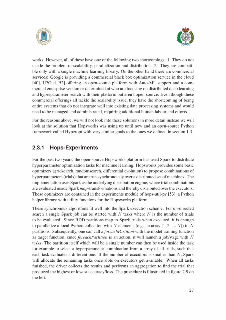
For the past two years, Hopsworks, an open-source machine learning platform, has used

Apache Spark to distribute hyperparameter optimization tasks in machine learning. Hops-

works provides some basic optimizers (grid-search, random-search, differential evolution)

to propose combinations of hyperparameters (trials) that are run synchronously in paral-

lel. However, many such trials perform poorly, and waste a lot of hardware accelerator

cycles on trials that could be stopped early, freeing up resources for other trials. In this

thesis, the work on Maggy is presented, an open-source asynchronous and fault-tolerant

hyperparameter optimization framework built on Spark. Maggy transparently schedules

and manages hyperparameter trials, enabling state-of-the-art asynchronous optimization

algorithms, thereby increasing resource utilization and increasing the number of trials that

can be performed in a given period of time up to 30% on a fixed amount of resources. Early

stopping is found to perform best when the model is sensitive, in terms of generalization

performance, to the hyperparameter configurations.

i

Dedication

This thesis is dedicated to my family: Karin, Kurt, Leonie, Ina, Lotta and Matthias.

ii

Acknowledgements

Firstly, I would like to thank my supervisor Alberto Mozo, Professor at E.T.S de Ing. de

Sistemas Informáticos UPM, for the remote supervision of my thesis.

Secondly, I thank my company supervisor Jim Dowling, Associate Professor at KTH ICT

school and CEO of Logical Clocks AB, for giving me the opportunity to join the team at

the company and for the help throughout the process of writing this thesis. Moreover, I

would like to thank my advisors at the company, Robin Andersson and Kim Hammar, for

constantly challenging my ideas and helping me get familiar with the Hopsworks platform.

Especially, Robin Andersson for his previous work done on the topic and his expertise on

Graphics Processing Units. The entire Logical Clocks team was always helpful and I would

like to thank them for the opportunity to present my work at their meetup in front of a big

audience, as well as for providing the computational resources to conduct the experiments.

Thirdly, I wish to thank my fellow students, colleagues, friends and family supporting me

along this project. Sina Sheikholeslami for the code and thesis reviews, my friends for

proof-reading the thesis and my family for the constant moral support.

Finally, I would like to thank EIT Digital for providing me with the possibility to complete

this study at two different universities, in two different countries, making countless new

friends and valuable experiences. It’s these kind of things that make me believe in the

concept of the European Union.

iii

Contents

1 Introduction 11.1 Hopsworks . . . . . . . . . . . . . . . . . . . . . . . . . . . . . . . . . 2

1.2 Problem Description . . . . . . . . . . . . . . . . . . . . . . . . . . . . 2

1.3 Goals . . . . . . . . . . . . . . . . . . . . . . . . . . . . . . . . . . . . 4

1.4 Purpose . . . . . . . . . . . . . . . . . . . . . . . . . . . . . . . . . . . 4

1.5 Hypothesis . . . . . . . . . . . . . . . . . . . . . . . . . . . . . . . . . 4

1.6 Boundaries . . . . . . . . . . . . . . . . . . . . . . . . . . . . . . . . . 4

1.7 Ethical, social and environmental aspects . . . . . . . . . . . . . . . . . 5

1.8 Structure . . . . . . . . . . . . . . . . . . . . . . . . . . . . . . . . . . . 6

2 Background 72.1 Automated Machine Learning . . . . . . . . . . . . . . . . . . . . . . . 7

2.1.1 Terminology and Definitions . . . . . . . . . . . . . . . . . . . . 8

2.1.2 Problem Setup: What to automate? . . . . . . . . . . . . . . . . 9

2.1.3 Automation techniques: How to automate? . . . . . . . . . . . . 12

2.2 Apache Spark . . . . . . . . . . . . . . . . . . . . . . . . . . . . . . . . 21

2.2.1 Architecture . . . . . . . . . . . . . . . . . . . . . . . . . . . . . 22

2.2.2 Driver - Executor Communication . . . . . . . . . . . . . . . . . 23

2.2.3 Execution scheduling . . . . . . . . . . . . . . . . . . . . . . . . 24

2.2.4 Spark and Distributed Deep Learning . . . . . . . . . . . . . . . 26

2.3 Related Work . . . . . . . . . . . . . . . . . . . . . . . . . . . . . . . . 26

2.3.1 Hops-Experiments . . . . . . . . . . . . . . . . . . . . . . . . . 27

2.3.2 Hyperopt . . . . . . . . . . . . . . . . . . . . . . . . . . . . . . 28

3 Methods 313.1 Research methods . . . . . . . . . . . . . . . . . . . . . . . . . . . . . . 31

3.2 Data Collection and Analysis . . . . . . . . . . . . . . . . . . . . . . . . 32

3.3 Open-Source Best Practices . . . . . . . . . . . . . . . . . . . . . . . . . 32

iv

3.3.1 Semantic versioning . . . . . . . . . . . . . . . . . . . . . . . . 32

3.3.2 License . . . . . . . . . . . . . . . . . . . . . . . . . . . . . . . 33

3.3.3 Documentation . . . . . . . . . . . . . . . . . . . . . . . . . . . 33

4 Design and Implementation 344.1 Motivation and Use Case . . . . . . . . . . . . . . . . . . . . . . . . . . 34

4.1.1 Scenarios . . . . . . . . . . . . . . . . . . . . . . . . . . . . . . 35

4.1.2 Requirements . . . . . . . . . . . . . . . . . . . . . . . . . . . . 36

4.2 Spark integration . . . . . . . . . . . . . . . . . . . . . . . . . . . . . . 36

4.3 Interfaces . . . . . . . . . . . . . . . . . . . . . . . . . . . . . . . . . . 38

4.3.1 User . . . . . . . . . . . . . . . . . . . . . . . . . . . . . . . . . 38

4.3.2 Developer . . . . . . . . . . . . . . . . . . . . . . . . . . . . . . 40

4.4 Architecture . . . . . . . . . . . . . . . . . . . . . . . . . . . . . . . . . 41

4.4.1 High level view . . . . . . . . . . . . . . . . . . . . . . . . . . . 41

4.4.2 Driver-side . . . . . . . . . . . . . . . . . . . . . . . . . . . . . 43

4.4.3 Executor-side . . . . . . . . . . . . . . . . . . . . . . . . . . . . 45

4.4.4 Communication . . . . . . . . . . . . . . . . . . . . . . . . . . . 46

4.4.5 Logging . . . . . . . . . . . . . . . . . . . . . . . . . . . . . . . 48

4.5 Failure assumptions and behaviour . . . . . . . . . . . . . . . . . . . . . 49

4.5.1 Executor failure . . . . . . . . . . . . . . . . . . . . . . . . . . . 49

4.5.2 Driver failure . . . . . . . . . . . . . . . . . . . . . . . . . . . . 51

4.6 Security . . . . . . . . . . . . . . . . . . . . . . . . . . . . . . . . . . . 51

4.7 Testing . . . . . . . . . . . . . . . . . . . . . . . . . . . . . . . . . . . . 52

5 Results and Analysis 535.1 Experiments . . . . . . . . . . . . . . . . . . . . . . . . . . . . . . . . . 53

5.1.1 Experimental Setup . . . . . . . . . . . . . . . . . . . . . . . . . 54

5.1.2 Hyperparameter Optimization Task . . . . . . . . . . . . . . . . 54

5.1.3 Neural Architecture Search Task . . . . . . . . . . . . . . . . . . 59

5.2 Validation and Discussion . . . . . . . . . . . . . . . . . . . . . . . . . 61

6 Conclusion 646.1 Future Work . . . . . . . . . . . . . . . . . . . . . . . . . . . . . . . . . 66

Bibliography 68

A Maggy Implementation Details 73A.1 API Details . . . . . . . . . . . . . . . . . . . . . . . . . . . . . . . . . 73

A.2 Diagrams . . . . . . . . . . . . . . . . . . . . . . . . . . . . . . . . . . 74

v

B Experiment Additions 78B.1 ASHA Experiment . . . . . . . . . . . . . . . . . . . . . . . . . . . . . 78

Glossary 81

Acronyms 83

vi

List of Figures

2.1 A typical machine learning pipeline . . . . . . . . . . . . . . . . . . . . 10

2.2 The subsets of Auto-ML . . . . . . . . . . . . . . . . . . . . . . . . . . 11

2.3 The human iterative optimization approach vs. black-box optimization . . 13

2.4 Greedy iterative approaches to hyperparameter optimization . . . . . . . 14

2.5 Comparison of grid and random-search . . . . . . . . . . . . . . . . . . 15

2.6 Reinforcement learning for Neural Architecture Search . . . . . . . . . . 18

2.7 Architecture of Apache Spark . . . . . . . . . . . . . . . . . . . . . . . . 23

2.8 Spark Tasks - runtime representation of RDD partitions . . . . . . . . . . 25

2.9 Synchronous hyperparameter optimization on Hopsworks with hops-util-py 28

2.10 Architecture of parallel distributed Hyperopt . . . . . . . . . . . . . . . . 29

4.1 Parallelization of black-box optimization . . . . . . . . . . . . . . . . . . 35

4.2 Spark inefficiency with asynchronous workloads . . . . . . . . . . . . . . 36

4.3 Unavailability of dynamic scheduling in Spark . . . . . . . . . . . . . . . 36

4.4 Maggy within Apache Spark . . . . . . . . . . . . . . . . . . . . . . . . 37

4.5 High-level architecture overview of Maggy . . . . . . . . . . . . . . . . 42

4.6 RPC communication within Maggy . . . . . . . . . . . . . . . . . . . . 47

4.7 UX of Maggy experiments in Jupyter . . . . . . . . . . . . . . . . . . . 48

5.1 Hyperparameter optimization results over time on cuda-convnet . . . . . 58

5.2 Neural architecture search results over time on CIFAR-10 . . . . . . . . . 61

A.1 Class diagram driver side of Maggy . . . . . . . . . . . . . . . . . . . . 75

A.2 Class diagram RPC module . . . . . . . . . . . . . . . . . . . . . . . . . 76

A.3 Starting a Maggy experiment at runtime . . . . . . . . . . . . . . . . . . 77

B.1 ASHA Experiment "Small CNN Architecture Tuning Task" . . . . . . . . 79

vii

List of Tables

4.1 The work to be executed by the worker thread depending on messages . . 44

4.2 Client to server communication protocol . . . . . . . . . . . . . . . . . . 47

5.1 Search space for the hyperparameter optimization task. . . . . . . . . . . 55

5.2 Hyperparameter optimisation task: Resource allocation for SHA . . . . . 56

5.3 Hyperparameter optimization task: Average results over three repeated

runs per optimizer with standard deviations in parentheses. . . . . . . . . 58

5.4 Search space for the neural architecture search task. . . . . . . . . . . . . 60

5.5 Neural architecture search task: Average results over three repeated runs

per optimizer with standard deviations in parentheses. . . . . . . . . . . . 61

B.1 Search space for the "small CNN architecture tuning task" of Li et al. [44] 78

B.2 ASHA Experiment "Small CNN Architecture Tuning" task: Average re-

sults over three repeated runs per optimizer. . . . . . . . . . . . . . . . . 79

viii

Chapter 1

Introduction

Unknowingly, machine learning (ML) has become part of our daily life in many ways. Be it

speech assistants, music recommendations or soon to be autonomous cars. We have seen

an explosion of ML research and applications, in specific, deep learning (DL) methods

have led to a drastic increase in performance of the models, e.g. AlphaZero by Google’s

DeepMind can now beat human world champions in the games of chess, shogi (Japanese

chess) and Go - all as a single system [1].

However, even though we often label these successes with the term artificial intelligence

(AI), building such systems requires a team of highly trained and specialized data scien-

tists and domain experts with human intelligence [2]. These teams have to make a plethora

of design decisions, significantly influencing the performance of the machine learning

methods. Particularly in deep learning [3], where model complexity grows quickly for

a learning problem, the experts have to decide on the right neural architectures, training

procedures, data preparation, regularization methods and hyperparameters of all of these

to produce the desired predictive power. Typically, hyperparameters are set statically, and

data scientists often have to perform tens or hundreds of experiments in a trial and er-

ror manner to find good parameters for their machine learning system. This makes the

development of machine learning pipelines an expensive and time consuming process.

Due to the growing amount of data needed to train good deep neural models, as deep

models work best with larger data sets, but also because of the complexity of the mod-

els itself, a lot of research effort was recently put into the development of efficient op-

timization algorithms and systems to distribute computations in a cluster of computers

in a scalable and fault-tolerant manner. As a result, the open-source distributed general-

purpose cluster-computing framework Apache Spark (Spark) [4], originally introduced by

Zaharia et al. [5], gained widespread popularity among data scientists. Spark offers a pro-

1

gramming interface to program entire clusters of computers with implicit data-parallel and

fault-tolerant applications. This is called horizontal scaling and proved to be a success for

data parallel tasks such as data preparation and iterative loops. Another way of scaling

is vertically, by adding more computational power to the same physical machine, which

has given rise to the usage of specialized hardware accelerators such as Graphics Process-

ing Units (GPUs), Tensor Processing Units (TPUs) and Field-Programmable Gate Arrays

(FPGAs). These accelerators are fast at embarrassingly parallel tasks such as matrix mul-

tiplications and therefore very popular and preferred for deep learning tasks. In particular,

GPUs are being adopted due to their good price/performance ratio, compared to the still

very expensive FPGAs. However, clusters of computers and their administration, espe-

cially with specialized hardware accelerators, are expensive and therefore efficient usage

is highly desirable.

This thesis tackles the efficiency of hyperparameter optimization tasks with a transparent

Python framework based on Apache Spark called Maggy.

1.1 Hopsworks

Hopsworks is a full-stack platform for data science built on HopsFS. HopsFS [6] is an

open-source distribution of the Apache Hadoop Distributed File System (HDFS) that keeps

metadata in a NewSQL database instead of in-memory on a single node, thereby mitigating

the main scalability bottleneck in HDFS, achieving a 16x higher throughput and scaling to

larger cluster sizes with significantly lower client latencies. Furthermore, the developers

of HopsFS made efforts to allow YARN to manage GPUs as a resource.

Hopsworks [7] is the front-end for HopsFS. Hopsworks integrates many popular platforms

such as Spark, Flink, Kafka, HDFS, and YARN, therefore making it easy for users to inter-

act with Hadoop. Hopsworks has unique support for project-based multitenancy, scale-out

ML pipelines and managed GPUs-as-a-resource, therefore, hiding the complexity of pro-

viding the scalability to the end-user, usually a data scientist.

1.2 Problem Description

The availability of means to combine horizontal and vertical scalability as described above,

offers the promise of reducing the time required to perform experiments, among others,

to find good hyperparameters or neural architectures, to be proportional to the availability

of hardware accelerators. That is, assuming the availability of tens or hundreds of GPUs,

2

it should be possible to parallelize experiments over all those GPUs using some supplied

search algorithm. Hyperparameter performance space is quite often not differentiable,

so gradient-based searches are typically not feasible. Instead, more robust (but less effi-

cient) methods such as random-walk, and grid-search are used. Other popular methods

are Bayesian Optimization [2] and Hyperband [8].

The search for good parameters resembles a black-box optimization problem with an ex-

pensive function to evaluate, which is the training of the model with a set of parameters or

an architecture [2]. The processes of evaluating the black-box function at different points

of the search space are independent and, therefore, the training of different models can be

scaled horizontally, by having each available machine train a different model, which will

be called a trial. Additionally, these machines can be scaled vertically by using GPUs.

However, many such trials perform poorly, and we waste a lot of CPU and hardware accel-

erator cycles on trials that could be stopped early. By stopping poor trials early, expensive

resources are freed up for other trials to explore the search space, allowing for a more

efficient use of resources.

Hence, the problem can be defined in two dimensions:

1. Algorithmic: A limitation of existing black-box optimization algorithms is that they

are typically stage or generation-based. For example, if genetic algorithms are used

for hyperparameter search, one has to wait for all models to finish in order to gen-

erate a new generation of potential parameters from the best performing individ-

uals. Hence, no new trial can be scheduled on the resource until the entire stage

of the algorithm finished. However, there are algorithms that do not suffer from

this synchronism but can be deployed asynchronously, that is, new hyperparameter

combinations can be produced independent of models currently being trained. The

research question in this dimension can be formulated as: Which algorithms can be

used asynchronously and how do they perform?

2. System: Apache Spark does not support asynchronous task scheduling, and there-

fore asynchronous algorithms and early stopping do not fit into the execution model

of Spark by default. For this side of the problem it is being asked: Can Spark be

leveraged to provide system support for fault-tolerant, asynchronous hyperparame-

ter optimization?

3

1.3 Goals

The main thrust of this project involves building platform and algorithmic support for

asynchronous hyperparameter optimization (HPO) and neural architecture search (NAS)

with Apache Spark, on the Hopsworks platform.

Hence, the project is successful if:

1. We can provide a simple API to end users to conduct HPO experiments.

2. We implement a framework to asynchronously schedule blackbox-optimization prob-

lems on an Apache Spark cluster.

3. We implement algorithms to leverage this system in order to early stop badly per-

forming model training.

1.4 Purpose

The purpose of this work is to evaluate a possible solution to reduce time spent for tuning

hyperparameters of machine learning models.

1.5 Hypothesis

Given a machine learning problem, tenths or hundreds of trials need to be performed

to find hyperparameters such that a machine learning model generalizes well on unseen

data. Many of such trials perform badly already early during training and can therefore be

stopped to save expensive computation time.

1.6 Boundaries

The developed solution will be tightly integrated with the Hopsworks platform and there-

fore will not be usable on any Spark cluster. This allows us to collect important meta data

about experiments, provide fault tolerance and track them during execution with Elastic

Search [9] and TensorBoard [10]. Nevertheless, an early version will be usable on any

4

Spark cluster and can be leveraged as a proof of concept and to create traction for the

project in the open-source community.

There are many asynchronous optimization algorithms which could profit from this frame-

work and could be implemented on top if it, however, research has shown that random

search is hard to beat [11] and since it is asynchronous by nature, this will be used as base-

line and other algorithms will be added as time permits. Since the work is released under

an open source license, the framework will instead provide an extensible and intuitive de-

veloper API, as we specified with goal (1) in section 1.3, to allow developers to implement

their own optimization algorithms.

1.7 Ethical, social and environmental aspects

From an ethical point of view, the use of a framework to speed up hyperparameter opti-

mization for machine learning does not pose any threats itself, but rather the applications

that machine learning is used for can be unethical. As the performance of the models in-

creases in terms of accuracy, so does the area where they can be applied. This includes

ethical use cases creating social value, such as cancer detection, but also ethically ques-

tionable applications, such as increasing marketing effectiveness for online-gambling busi-

nesses. Therefore, practitioners and companies need to make sure they use the technology

in a responsible way.

Another social aspect includes data privacy, which plays a role as soon as data leaves secure

system environments. To conduct this research and build the described system, data needs

to be transferred across a network which might be intersected by adversaries. However,

the content of the data itself is not sensitive with respect to the disclosure of individuals,

hence we are not at risk from that perspective. Nevertheless, measures are taken to make

the system as secure as possible, more about these measures for the security of this work

is described in section 4.6.

Nowadays, a considerable amount of energy is spent on computational power. The recent

past has shown that deep learning accuracy mainly increases with the use of more data,

which on the other hand requires more computational power and hence also more energy.

Therefore, from an environmental perspective it makes sense to invest into research to

make more efficient use of resources.

5

1.8 Structure

Firstly, a background section is following to introduce terminology adopted and needed

throughout the rest of the report. Furthermore, the information needed to comprehend

the thesis is provided as well as an overview of the state-of-the-art in the field. Having

set the scope and background, a chapter on the development and research methods con-

ducted throughout the project is presented. This is followed by a chapter dedicated to the

description of the implementation of this project - a python framework for asynchronous

hyperparameter optimization on Apache Spark. The chapter describes the requirements,

architecture and design of the software system and a justification of the design decisions

made. Subsequently, we present the results of experiments conducted to approve or reject

our research hypothesis. Finally, the thesis is concluded by a chapter to summarize the

results, show future research directions and elaborate on weaknesses and future work to

be done on the framework.

6

Chapter 2

Background

To set the context of this thesis, this chapter will introduce important concepts and a lit-

erature review on the subject matter. Firstly, there is a section defining the more general

concept of automated machine learning (Auto-ML) and some terms and concepts related to

machine learning and hyperparameter optimization (HPO) in order to set common ground.

Possible points for automation in machine learning pipelines are investigated and is fol-

lowed by a introduction of hyperparameter optimization and its current state-of-the-art.

This section will also highlight the importance of hyperparameter optimization and there-

fore further motivate this project. Neural Architecture Search (NAS) will be presented

as a special case of HPO providing more use cases for the output of this project. Sub-

sequently, the architecture of Apache Spark will be presented in detail, since the project

builds on Spark as a back-end. This section will highlight the mismatch between asyn-

chronous scheduling and the nature of Sparks execution schemes. The last section of this

chapter will cover related work to the topic, showing that other parties are working on

similar solutions, but highlighting the differences and uniqueness of this project.

2.1 Automated Machine Learning

Not only do machine learning experts have to make decisions on the algorithms they use

in their machine learning pipelines, but also each of these algorithms comes with a set

of hyperparameters, that have to be tuned to find settings that produce well generalizing

models. The field of automated machine learning or short Auto-ML aims to make these

decisions in an organized and automated fashion, that is, data-driven and based on an ob-

jective metric without human input [2]. Auto-ML promises to provide machine learning to

7

domain experts without deep knowledge of ML itself. Having data at hand, the user simply

feeds it into the Auto-ML system, which in turn will take all decisions for him, returning

the approach best suitable for the specific learning problem. Hutter, Kotthoff, and Van-

schoren [2] show in their book that Auto-ML approaches are very mature and can compete

with, sometimes even outperform, human machine learning experts. Furthermore, recent

methods have shown that resource requirements for Auto-ML applications can be reduced

from several hours to few minutes [2]. When speaking about performance of supervised

machine learning models in this thesis, it is referred to the generalization error, that is the

error made when predicting outcome values for previously unseen data (also known as

out-of-sample error). In line with these developments, Yao et al. [12] define three core

goals of Auto-ML:

1. Good generalization capabilities across various data inputs and learning tasks.

2. No human input requirements, the machine learning tool is configured by the system

itself.

3. The system should be efficient to produce reasonable outputs within a limited bud-

get.

Furthermore, Yao et al. [12] introduce a taxonomy for the classification of Auto-ML prob-

lems in their extensive literature study. They divide the problem into two questions:

1. What to automate? (The problem setup)

2. How to automate? (Techniques applicable)

A literature review is conducted along this taxonomy in the following subsections.

2.1.1 Terminology and Definitions

The research and industrial community has silently agreed and adopted some terminology

and definitions with only slight variations to describe problems and concepts in the field

of Auto-ML. To be on a common page, this section shortly defines this terminology and

how it is being adopted throughout this thesis.

1. Hyperparameter: A hyperparameter in machine learning, is a parameter that needs

to be set manually, usually by an expert, before the learning process begins. This

distinguishes it from other parameters that are to be learned through the model itself.

2. Search Space: A search space is a combination of multiple hyperparameters given

their feasible regions.

8

3. Experiment: Given a search space, objective and a black-box function, usually the

model training procedure, an experiment is the whole process of finding the best

hyperparameter combination in the search space, that is, optimizing the black-box

function with respect to the objective.

4. Suggestion: A suggestion is a hyperparameter combination sampled from the search

space, that should be promising, in terms of performance, and therefore evaluated

next. Suggestions are generally produced by some specified search algorithm, for

example Bayesian optimization or simple random search.

5. Trial: A trial is the process of evaluating the black-box function at a point in the

search space (suggestion/sample). The trial object contains all information related

to the execution and evaluation of a suggestion.

6. Optimizer: The optimizer implements the logic of generating trials/suggestions

from the search space based on past realisations and an optimization model. This

optimizer is not to be confused with the optmization algorithm used to train the

model itself.

2.1.2 Problem Setup: What to automate?

This section looks at question (1) defined in section 2.1 and the following subsections focus

on question (2).

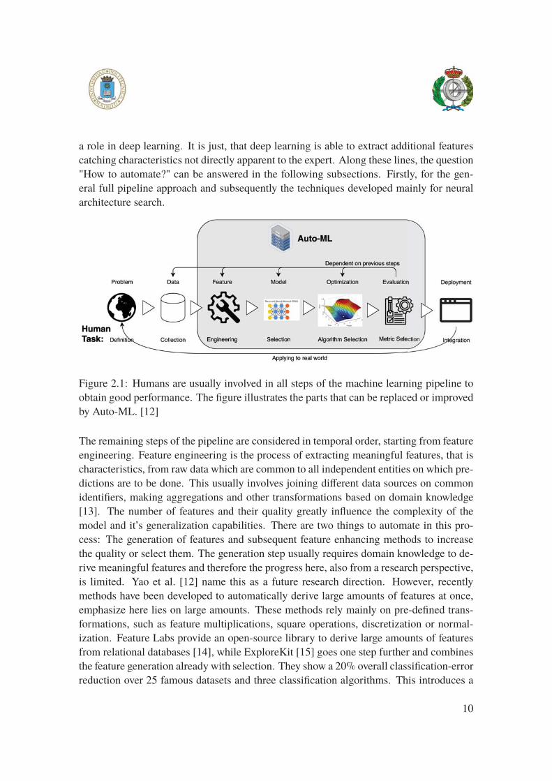
Figure 2.1 illustrates the steps of a typical machine learning pipeline and the decisions

that can potentially be replaced by an Auto-ML system. There are steps that can not be

replaced by an Auto-ML system such as the definition of the problem or the integration

and collection of data sources. This is due to the need of domain knowledge and the

connection to the real world. Furthermore, the deployment of the final model has to be

done by engineers, since existing systems are usually complex and highly use case driven.

However, additional to the selection of the model and the setting of its hyperparameters,

there are other design decisions that influence the final model performance, and research

is proposing methods to automate them. Yao et al. [12] split the problem setup in their

taxonomy into two sub-problems. Firstly, the full scope general ML pipeline consisting

of three parts: feature engineering, model selection and algorithm selection, concerning

mainly traditional machine learning approaches like support vector machines and random

forests. The second sub-problem, which presents itself as a special case of the previous

one is deep learning. In deep learning all these three steps are partly integrated and config-

ured in the neural network architecture itself. Therefore, it becomes a problem of neural

architecture search. Nevertheless, good core features and feature engineering still plays

9

a role in deep learning. It is just, that deep learning is able to extract additional features

catching characteristics not directly apparent to the expert. Along these lines, the question

"How to automate?" can be answered in the following subsections. Firstly, for the gen-

eral full pipeline approach and subsequently the techniques developed mainly for neural

architecture search.

Figure 2.1: Humans are usually involved in all steps of the machine learning pipeline to

obtain good performance. The figure illustrates the parts that can be replaced or improved

by Auto-ML. [12]

The remaining steps of the pipeline are considered in temporal order, starting from feature

engineering. Feature engineering is the process of extracting meaningful features, that is

characteristics, from raw data which are common to all independent entities on which pre-

dictions are to be done. This usually involves joining different data sources on common

identifiers, making aggregations and other transformations based on domain knowledge

[13]. The number of features and their quality greatly influence the complexity of the

model and it’s generalization capabilities. There are two things to automate in this pro-

cess: The generation of features and subsequent feature enhancing methods to increase

the quality or select them. The generation step usually requires domain knowledge to de-

rive meaningful features and therefore the progress here, also from a research perspective,

is limited. Yao et al. [12] name this as a future research direction. However, recently

methods have been developed to automatically derive large amounts of features at once,

emphasize here lies on large amounts. These methods rely mainly on pre-defined trans-

formations, such as feature multiplications, square operations, discretization or normal-

ization. Feature Labs provide an open-source library to derive large amounts of features

from relational databases [14], while ExploreKit [15] goes one step further and combines

the feature generation already with selection. They show a 20% overall classification-error

reduction over 25 famous datasets and three classification algorithms. This introduces a

10

new challenge and the need for feature enhancing methods. As the number of features

grows, so does the complexity of the model and the model therefore tends to over-fit the

training data points, meaning that it predicts the points that it was trained with well but

generalizes poorly on unseen data. Therefore, data scientists spend a great amount of time

subsequently selecting the features producing the lowest generalization error.

The selection of features can be performed in a time consuming trial and error manner or

recent models are able to incorporate that step into the model itself and therefore making

it a hyperparameter tuning problem. One such method is the application of regularization

methods to shrink coefficients of features that don’t add predictive power towards zero,

therefore limiting their influence on predictions, reducing the variance as well as the com-

plexity of the model [16]. These methods then introduce a hyperparameter to control the

regularization strength, which in turn can be tuned. Another approach is feature projection

into lower dimensional spaces such as Principal Component Analysis [13], however, also

here the user needs to decide on the number of components to retain, therefore, introduc-

ing a hyperparameter. This shows that feature engineering can be made a hyperparameter

optimization problem by incorporating the selection into the model. However, even if the

data scientist follows a trial and error approach, the decision of taking a feature into the

model can be encoded in a binary hyperparameter, therefore making it a HPO problem.

Figure 2.2: Hyperparameter optimization and neural architecture search as sub-fields of

Auto-ML.

While, the previous overview holds for classical machine learning approaches, with deep

neural networks, features extraction is usually incorporated into the model itself with au-

toencoders to reduce dimensionality in data, word embeddings for language modelling or

convolutional models for image data [17]. However, designing such architectures for deep

learning is difficult. Among others practitioners have to decide on the number of layers

and neurons, activation functions and dropout rates [18] but these can be modelled as hy-

perparameters too. 2.2 shows the relation of Auto-ML, hyperparameter optimization and

NAS.

11

According to the No Free Lunch Theorems of Wolpert and Macready [19] there is no su-

pervised learning algorithm that is superior on all possible learning tasks in the model

selection step. In practice, finding even an algorithm that performs best on a small set of

tasks is already hard. This means, with every new learning task, a data scientist has to

try different approaches and compare. There are models known to perform well on cer-

tain tasks. Therefore, data scientists usually find suitable models fast, but every model

comes with hyperparameters to be set in order to achieve the best possible generalization

error. Hence, HPO is a crucial step at this point. Another approach, often called ensem-

ble approach, requires to train many different models and subsequent combination of the

predictions, for example in the form of random forests [13].

The last and most time-consuming step of the actual learning process is the training or

optimization of the model on training data. Hence, the selection of the algorithm can in-

fluence the resource demand but it also impacts the performance of the final model [20].

There is usually a trade-off between resource demand and performance involved. For ex-

ample, in Stochastic Gradient Descent [21] single iterations are very cheap but in order

to converge to an optimum, one needs to perform many of them. Hence, it becomes a

question of when to stop. As with model selection, the search space for the optimization

algorithm consists of the decision on the algorithm itself and its parameters.

Finally, the evaluation of the model highly depends on the metric chosen. Often the metric

is also dependent on the problem to be solved and hence this decision can’t be automated

and has to be made by a human. If you want to detect cancer, for example, you want

to avoid false positives under all circumstances, therefore it would be the wrong metric.

However, once the metric is selected it can be used to optimize the rest of the pipeline in

an iterative approach, or with the help of some black-box optimization algorithm or search

algorithm.

2.1.3 Automation techniques: How to automate?

Following the taxonomy of Yao et al. [12], this section firstly considers the "How to au-

tomate?" question for the full pipeline problem, that is traditional models with the steps:

feature engineering, model selection and algorithm selection. Most of these techniques

will be applicable to neural architecture search if architectural design decisions are treated

as hyperparameters. Methods proven to be suitable mainly for deep learning will be dis-

cussed in a separate section. This is in line with a recent survey on Auto-ML by Zöller and

Huber [22]. It was already briefly discussed how feature engineering automation can be

turned into a problem of hyperparameter optimization, hence further details on that step

are not presented, since all following methods will be applicable to this as well.

12

The first step is the design of the ML pipeline. Zöller and Huber [22] find in their survey

that there is a lot of research around the pipeline design problem for neural networks, but

no publications treating the definition of general pipelines with classical models. They

argue that most approaches assume a best practice pipeline as the one outlined in figure

2.1. There were methods proposed based on genetic programming [23] or with the recent

success of reinforcement learning [1] self-play algorithms [24] have gained attention. With

this approach the model plays against itself, taking decisions on whether to extend or shrink

a pipeline. However, both these approaches suffer from expensive optimization, genetic

programming because of the expensive function evaluations [25] and self-play due to its

slow convergence [26]. For these reasons, throughout the rest of this thesis a static machine

learning pipeline as illustrated in figure 2.1 is assumed. Hence, the problem is narrowed

down to HPO.

Hyperparameter Optimization

The concept of HPO is not a new concept and was tackled by research already in the 1990s

as it was discovered that different hyperparameter combinations work best on different

datasets [27]. Also due to the No Free Lunch theorem [19], it is widely accepted that there

is no default hyperparameter set for algorithms that can’t be outperformed with HPO given

a specific learning task [2].

Figure 2.3: The iterative optimization loop, adopted by most practitioners (left) and its

parallels to black-box optimization (right).

Human ML experts tackle HPO in an iterative trial and error approach as shown in the left

of figure 2.3. They decide on a learning algorithm, set the parameters based on their ex-

pertise in order to subsequently train the model. When the training finished they validate

the performance on unseen data to update their belief about the hyperparameters and con-

tinue in this way. Not only is this process slow, because the training of the model is time

consuming, but it also leads to local optima since this approach is greedy. Humans usually

only update one parameter at a time because they believe to have found a good setting for

the others, therefore neglecting the dependence of the parameters. This greediness leads

to local optima as illustrated by figure 2.4.

13

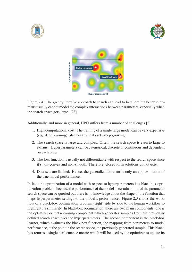
Figure 2.4: The greedy iterative approach to search can lead to local optima because hu-

mans usually cannot model the complex interactions between parameters, especially when

the search space gets large. [28]

Additionally, and more in general, HPO suffers from a number of challenges [2]:

1. High computational cost: The training of a single large model can be very expensive

(e.g. deep learning), also because data sets keep growing.

2. The search space is large and complex. Often, the search space is even to large to

exhaust. Hyperparameters can be categorical, discrete or continuous and dependent

on each other.

3. The loss function is usually not differentiable with respect to the search space since

it’s non-convex and non-smooth. Therefore, closed form solutions do not exist.

4. Data sets are limited. Hence, the generalization error is only an approximation of

the true model performance.

In fact, the optimization of a model with respect to hyperparameters is a black-box opti-

mization problem, because the performance of the model at certain points of the parameter

search space can be queried but there is no knowledge about the shape of the function that

maps hyperparameter settings to the model’s performance. Figure 2.3 shows the work-

flow of a black-box optimization problem (right) side by side to the human workflow to

highlight its similarity. In black-box optimization, there are two main components, one is

the optimizer or meta-learning component which generates samples from the previously

defined search space over the hyperparameters. The second component is the black-box

learner, which evaluates the black-box function, the mapping from parameters to model

performance, at the point in the search space, the previously generated sample. This black-

box returns a single performance metric which will be used by the optimizer to update its

14

knowledge about the search space to subsequently produce a sample that ideally has a

higher expected performance than the previous sample. This process is repeated until a

certain performance is reached or until the algorithm finds an optimum, which can be local

or global.

Black-box optimization tries to solve the challenges above by applying less efficient but

more robust algorithms. Therefore, any black-box optimization algorithm implemented in

the optimizer component, can also be applied to HPO.

Simple un-directed search:

The most straightforward and widely used algorithms for HPO are un-directed search tech-

niques, sometimes also called model free optimization [2]. They are un-directed because

they do not take into account the information gained through evaluating previous hyper-

parameter combinations. These algorithms have in common that they evaluate the black

box function at a certain number of samples from the search space independently, followed

by an aggregation step to find the combination that produces the minimum or maximum

performance. Since the combinations are not related to each other, these trials can be

evaluated in parallel.

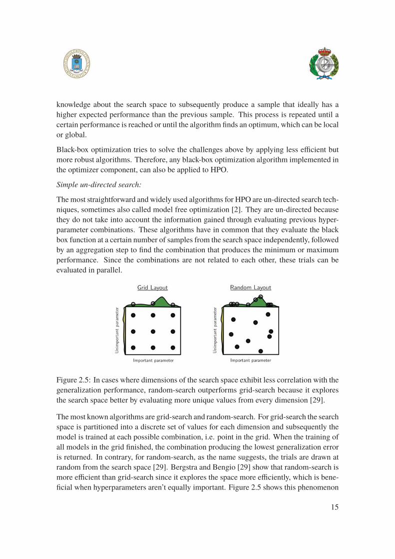
Figure 2.5: In cases where dimensions of the search space exhibit less correlation with the

generalization performance, random-search outperforms grid-search because it explores

the search space better by evaluating more unique values from every dimension [29].

The most known algorithms are grid-search and random-search. For grid-search the search

space is partitioned into a discrete set of values for each dimension and subsequently the

model is trained at each possible combination, i.e. point in the grid. When the training of

all models in the grid finished, the combination producing the lowest generalization error

is returned. In contrary, for random-search, as the name suggests, the trials are drawn at

random from the search space [29]. Bergstra and Bengio [29] show that random-search is

more efficient than grid-search since it explores the space more efficiently, which is bene-

ficial when hyperparameters aren’t equally important. Figure 2.5 shows this phenomenon

15

graphically. Researchers proposed approaches to make grid-search adaptive by creating a

more fine grained grid around well performing combinations [30]. Nevertheless, random-

search has a number of additional advantages: 1. Experiments can be extended by simply

drawing more random samples and evaluating them when more computational power be-

comes available. 2. If trials fail, the experiment results are still valid. The failed trial does

not leave a hole in the grid. 3. The feasible intervals of the hyperparameters in the search

space can be adjusted.

However, with a growing amount of dimensions (hyperparameters) in the search space,

these approaches suffer from the curse of dimensionality and need to evaluate an expo-

nential number of configurations to gain reasonable performance [22].

To conclude, since in both approaches trials are independent of each other, both algorithms

can be deployed asynchronously for the case when trials have different optimization times.

Additionally, random search has the advantage that if some trials finish much faster than

others, simply more samples can be drawn from the search space, therefore allowing to

evaluate more trials.

Directed adaptive search and optimization:

One class of directed search strategies is inspired by biological evolution. So called genetic

algorithms possess wide applicability to black-box optimization problems and fall into the

category of heuristic search [12]. These algorithms maintain a population of N configu-

rations, which are being evaluated and subsequently the best performing ones are selected

for the next generation and are either being combined (cross-over) or locally mutated for

the next iteration. Mutation and cross-over is needed to introduce new configurations,

therefore, creating a trade-off between exploration of new configurations and exploitation

of the good ones. While these methods have been used for feature selection [31] and in

NAS already decades ago [32], for general hyperparameter optimization, to the best of our

knowledge, there are no publications available. These algorithms are easily parallelized

within a generation, that is with a concurrency degree up to N , however, across genera-

tions the algorithm is synchronous and has to wait until a generation finishes to start a new

one and therefore it can’t be deployed asynchronously.

Genetic algorithms are directed but do not take the full feedback into account, an opti-

mization technique that tries to model all information available is Bayesian Optimization.

Bayesian Optimization proved to be the state-of-the-art algorithm for global optimization

in black-box settings [2]. Bayesian Optimization is modelling the mapping of samples of

the search space to their associated realised model performance with probabilities, given

the feedback of the black-box (model training). Gaussian processes [33] or Parzen Tree

Estimators [34] are popular approaches to model these probabilities. Every time an eval-

16

uation finishes, the probability distribution over the search space is being updated, such

that a new sample can be drawn with an acquisition function, for example to maximize ex-

pected improvement. A recent addition to this family of search optimization techniques,

named Fabolas, have shown improve the efficiency drastically [35], outperforming multi-

fidelity such as the Hyperband algorithm [8], which is described in section 2.1.3. Fabolas

extends Bayesian approaches to model loss and training time simultaneously as a func-

tion of the size of the data set. Thereby, it is able to automatically decide on the trade off

between information gain on one hand and computational cost on the other hand. Addi-

tionally, Bayesian Optimization suffers from a cold start problem, that is, in the beginning

of an experiment a few trials have to be generated at random in order to initialize the al-

gorithm. Nevertheless, once it is initialized, this algorithm can be operated completely

asynchronously in parallel because every time a trial finishes, the distribution can be up-

dated to generate a new trial.

Neural Architecture Search

Let us know consider neural architecture search as a special case of hyperparameter opti-

mization. For deep neural networks, which are artificial neural networks with more than

one hidden layer, the candidate architectures can quickly grow exponentially. A network

with 10 layers, can take more than 1010 different shapes.

Using evolutionary algorithms to produce neural architectures dates far back [32], but only

recently with the increase of computational power available, these methods were able to

produce results comparable to architectures designed by humans [36]. Real et al. [36] use

repeated, pair-wise competitions of random individuals instead of a standard generation

based evolution, making it a case of a tournament selection algorithm [37]. This means at

each evolutionary step, two random individuals are selected from a previously initialized

random population. These two individuals are compared and the worse one is immediately

removed from the population. The selected one instead is mutated and will be evaluated

(trained) in order to become a parent in the next iterations. Interestingly, this allows the

algorithm to operate asynchronously, since a worker can pick two individuals at any time

and is not bound to generations. This eliminates the previously mentioned shortcoming of

generation-based algorithms. In the initial population, Real et al. [36] start with simple one

layer networks, in order to analyse if the method is able to come up with good architecture

completely by itself. In their empirical evaluation Real et al. [36] conclude that this method

is able to construct accurate architectures on challenging problems with large search spaces

and from simple one layer networks, given that there are enough computational resources

available. Another advantage of their approach is that the final result will contain the fully

trained model. However, they highlight that future research should focus on making the

17

process more efficient to make it a viable option to replace human experts.

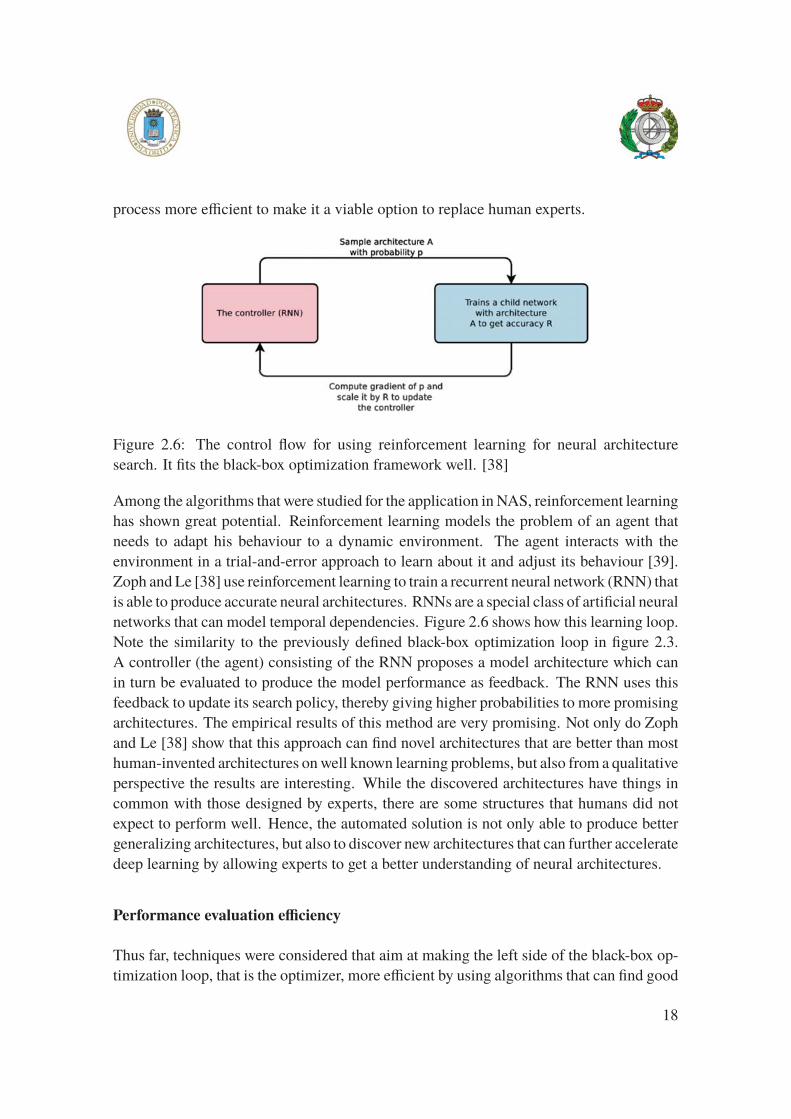
Figure 2.6: The control flow for using reinforcement learning for neural architecture

search. It fits the black-box optimization framework well. [38]

Among the algorithms that were studied for the application in NAS, reinforcement learning

has shown great potential. Reinforcement learning models the problem of an agent that

needs to adapt his behaviour to a dynamic environment. The agent interacts with the

environment in a trial-and-error approach to learn about it and adjust its behaviour [39].

Zoph and Le [38] use reinforcement learning to train a recurrent neural network (RNN) that

is able to produce accurate neural architectures. RNNs are a special class of artificial neural

networks that can model temporal dependencies. Figure 2.6 shows how this learning loop.

Note the similarity to the previously defined black-box optimization loop in figure 2.3.

A controller (the agent) consisting of the RNN proposes a model architecture which can

in turn be evaluated to produce the model performance as feedback. The RNN uses this

feedback to update its search policy, thereby giving higher probabilities to more promising

architectures. The empirical results of this method are very promising. Not only do Zoph

and Le [38] show that this approach can find novel architectures that are better than most

human-invented architectures on well known learning problems, but also from a qualitative

perspective the results are interesting. While the discovered architectures have things in

common with those designed by experts, there are some structures that humans did not

expect to perform well. Hence, the automated solution is not only able to produce better

generalizing architectures, but also to discover new architectures that can further accelerate

deep learning by allowing experts to get a better understanding of neural architectures.

Performance evaluation efficiency

Thus far, techniques were considered that aim at making the left side of the black-box op-

timization loop, that is the optimizer, more efficient by using algorithms that can find good

18

parameters with evaluating less trials. This section is dedicated to techniques for improv-

ing the efficiency of the black-box learner itself. Two possible solutions will be presented:

1. Early stopping of trials. 2. Algorithms that adapt resources of trials according to their

performance, so called multi-fidelity methods. One can think of multi-fidelity methods as

if they have early-stopping integrated by default, sometimes also called principled early

stopping.

By adding any of these two methods to a synchronous algorithm, the need for an asyn-

chronous mechanism for producing new trials arises, else it does not make sense from

an efficiency point of view. Hence, stopping a trial early, the algorithm needs to be able

to produce a new configuration right away without waiting for other trials. As outlined

before, random-search and Bayesian optimization are examples of such algorithms.

Early stopping:

Early stopping methods can be categorized in two classes: 1. Heuristics that take only

information about the trial itself into consideration in deciding whether to stop the trial in

questions and 2. methods taking into account all available information, that is, of trials

currently in the process of being trained and previously finalized trials. When speaking

about information of the performance of trials, it is being referred to the learning curve,

that is the error, loss or accuracy tracked over the time of training.

Let’s consider the first case: It is common practice to early stop model training when

the validation loss does not decrease for a specified number of iterations or even starts to

increase, indicating over-fitting. Furthermore, some hyperparameter settings can make a

model diverge instead of converging during optimization, this case can easily be detected

by only looking at the learning curve of the single trial.

While the first case is mainly used to prevent over-fitting, the second case is more com-

plicated but also more interesting to reduce training time: A heuristic called the Median

Stopping Rule implements the simple strategy of stopping a trial if its current performance

during training falls below the median of other previously finalized trials at similar points

in time of training. This strategy does not depend on a parametric model and therefore

does not introduce more hyperparameters. Golovin et al. [40] use this rule in their Vizier

black-box optimization service at Google and argue that due to its generality it is applicable

to a wide range of learning curves. This rule assumes that information about the learning

curves of all previous trials is available, for which a special mechanism is needed, in order

to centrally manage the execution of trials and collect the information.

An alternative global stopping rule is based on extrapolation of the performance learn-

ing curves of trials in order to make a prediction for the final performance value [41].

Given the set of finalized trials, a regression is performed in order to subsequently make

19

a prediction for the partial curves of trials currently in training. Given the current optimal

value, if the probability of a trial to exceed this optimal value is below a threshold, the trial

should be stopped early. Domhan, Springenberg, and Hutter [41] use Bayesian paramet-

ric regression, while Google Vizier [40] uses a Gaussian process model with a specially

designed kernel to measure similarity between learning curves. Moreover, Google has

found that this approach is applicable to a wider range of learning curves and is more ro-

bust to those other than hyperparameter tuning. They note that it surprisingly also works

well if the performance curve does not measure the same metric as objective value of the

model optimization. More recent approaches [42] use Bayesian neural networks exploit-

ing its flexibility by adding a learning curve layer building on the approach of [41]. This

method outperforms the Bayesian parametric regression [41] for predicting entirely new

curves, but also for extrapolating partial learning curves, especially when the curves have

not started to converge yet.

The disadvantage of learning curve prediction compared to the median stopping rule, is

its relative expensiveness in terms of the computational complexity. A model needs to be

learned and updated for the predictions. This can become a problem when the system is

supposed to be fault-tolerant, as the learning curve model possesses a state. In contrary,

the median rule only does comparisons and median computations and therefore does not

necessarily have to retain a state.

Multi-fidelity methods:

Multi-fidelity approaches try to approximate the performance of a model by only training

it with a constrained resource. The resource can be the amount of data, the number of

training iterations or epochs for neural networks or the number of features. The goal is

to give more resources to hyperparameter combinations that are promising in order to

produce robust results.

Jamieson and Talwalkar [43] propose a method called Successive Halving based on bandit

learning. The algorithm follows simple logic. Initially n random combinations are drawn

from the search space, of which each is trained with a fraction 1/n of the total resources

available. Subsequently, as the name suggests, the best performing half of the trials is

promoted to the next iteration, also called rung, with twice the initial budget allocated.

This procedure is repeated until only one trial remains. The rationale behind this logic

is that good trials receive exponentially more training time than bad ones. Jamieson and

Talwalkar [43] show empirically that this yields generalization errors comparable to base-

line methods but in significantly shorter experiment time. However, one limitation of the

algorithm is that it introduces a new hyperparameter, n, that has to be selected. This poses

a trade-off between exploration and more robust results. Choosing a larger n to start with

covers more areas of the search space, increasing the initial probability of finding a point

20

close to a global optimum, but the approximation with the low resource might change over

the course of the experiment.

Addressing the shortcoming of the previous algorithm, Li et al. [8] propose a modification

to successive halving called Hyperband. They reason that if randomly selected configura-

tions perform similarly well and converge slowly, then you would start the experiment with

a small number n of, while with fast model convergence, you could start a large number

of trials in the first iterations, therefore fully exploiting your budget. Based on this obser-

vation, they propose to loop over multiple different values for n, which they call brackets,

while keeping the budget fixed. Essentially treating n as a new hyperparameter and per-

forming grid-search over feasible values. In their empirical evaluations they find that with

increasing number of dimensions in the search space, the most exploratory brackets (large

n) perform best. Hence, especially for neural architecture search, Successive Halving with

large n is sufficient.

Regarding the parallelization of the previous two approaches, both suffer from a major

problem. Assuming the availability of many workers, each of which can train a single

model at a time, as the number of configurations is halved at every iteration, once the

number of trials in an iteration is below the number of available workers, some resources

will be idle. A recent publication by Li et al. [44] addresses this issue and also the short-

coming of selecting an appropriate n. The Asynchronous Successive Halving Algorithm

(ASHA) [44] changes the Successive Halving algorithm by promoting trials bottom up to

the next rung whenever possible instead of waiting until a wide set of trials finished in

the first iteration. ASHA starts by assigning workers to add configurations to the lowest

rung with the lowest resource. As workers finish and request a new trial, ASHA looks at

the rungs from bottom up to see if there are trials in the top 1/η, where η is the reduction

factor, which does not have to be 2 as in the case of successive halving. If no configuration

can be promoted, the worker will grow the lowest rung so that subsequently more trials

can be promoted. This asynchronism allows near 100% resource utilization, while eval-

uating more trials and therefore exploring the search space more. Li et al. [44] show that

this method scales linearly with the number of workers and therefore is superior to other

state-of-the-art methods especially when many workers are available.

2.2 Apache Spark

"Apache Spark is a unified analytics engine for large-scale data processing." [4]. It is based

on a distributed memory abstraction developed by Zaharia et al. [5] in 2012 and it is called

unified because this abstraction can be used for ETL, batch and stream analytics, machine

21

learning and graph processing. It offers rich high-level application programming inter-

faces (APIs) in various programming languages: Scala, Java, R, SQL and Python, also

called PySpark. One of the main goals of this project was to create a framework that runs

on top of Apache Spark. The reason for that being that Spark became the industry stan-

dard for data intensive computing, got adopted by many corporations and we do not want

to add additional administration overhead for a new system. A data scientist who is com-

fortable working with Python or even PySpark should be able to use the framework with

the lowest possible barrier to get started. Many surveys find Python to be the most popular

programming language among data scientists1, further motivating the use of Python for

the proposed solution.

This section is mainly based on "The Internals of Apache Spark" gitbook by Laskowski

[45]. He provides a detailed description of the low-level internals of the Apache Spark

Core. Furthermore, the official documentation and programming guides of Spark [4]

served as a source for these descriptions.

2.2.1 Architecture

Spark utilizes a master/worker setup. A Spark application runs as an independent set of

Java Virtual Machine (JVM) processes on a cluster of computers, which get coordinated

by the so called SparkContext object in the main program. The main program with the

SparkContext is called the driver and builds the entry point to the programming interfaces

of Spark. The Spark application is alive as long as the SparkContext exists. The driverconnects to a cluster manager, also called master, to request resources, i.e. processes, on

the worker machines. Spark comes with a standalone cluster manager but it also supports

external resource managers. Hopsworks uses a modified version of Hadoop’s Yet Another

Resource Negotiator (YARN) [46] [47] that is able to treat and isolate GPUs as a resource.

YARN is responsible for managing resources of a cluster by allocating them as containers

or processes to applications. Once the driver got allocated the required resources, it can

start executors on the worker nodes. Executors are responsible for doing the computa-

tional work and run in separate JVMs. This means each application has its own executor

processes to isolate them from each other, but it also means that there is no possibility to

share data between Spark applications (instances of SparkContext).

It is possible to run driver and executors all on the same physical machine (horizontal

cluster), on separate machines (vertical cluster) or a mix, meaning one can run multiple

executors on the same physical machine if enough resources are available. Typically, the

1https://www.kdnuggets.com/2017/01/most-popular-language-machine-learning-data-science.html

22

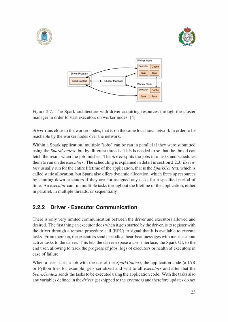
Figure 2.7: The Spark architecture with driver acquiring resources through the cluster

manager in order to start executors on worker nodes. [4]

driver runs close to the worker nodes, that is on the same local area network in order to be

reachable by the worker nodes over the network.

Within a Spark application, multiple "jobs" can be ran in parallel if they were submitted

using the SparkContext, but by different threads. This is needed to so that the thread can

fetch the result when the job finishes. The driver splits the jobs into tasks and schedules

them to run on the executors. The scheduling is explained in detail in section 2.2.3. Execu-tors usually run for the entire lifetime of the application, that is the SparkContext, which is

called static allocation, but Spark also offers dynamic allocation, which frees up resources

by shutting down executors if they are not assigned any tasks for a specified period of

time. An executor can run multiple tasks throughout the lifetime of the application, either

in parallel, in multiple threads, or sequentially.

2.2.2 Driver - Executor Communication

There is only very limited communication between the driver and executors allowed and

desired. The first thing an executor does when it gets started by the driver, is to register with

the driver through a remote procedure call (RPC) to signal that it is available to execute

tasks. From there on, the executors send periodical heartbeat messages with metrics about

active tasks to the driver. This lets the driver expose a user interface, the Spark UI, to the

end user, allowing to track the progress of jobs, logs of executors or health of executors in

case of failure.

When a user starts a job with the use of the SparkContext, the application code (a JAR

or Python files for example) gets serialized and sent to all executors and after that the

SparkContext sends the tasks to be executed using the application code. With the tasks also

any variables defined in the driver get shipped to the executors and therefore updates do not

23

get communicated back to the driver program. If multiple tasks use the same variables,

they get transferred multiple times. It would be inefficient to provide read-write shared

variables across tasks, but Spark provides instead two limited ways of communication

through shared variables:

1. Broadcast variables: A read-only variable that gets cached one time on each ma-

chine instead of sending it with every task.

2. Accumulators: A write-only (for executors) variable that is only modified through

an associative and commutative operation and is read-only for the driver. Accumu-

lators are designed to be used safely and efficiently in parallel and are mainly meant

for counters and accumulators. For example, Spark uses accumulators internally to

track job progress. Custom accumulators are possible but the limitation of associa-

tive and commutative operations still applies.

The broadcast and accumulator variables are the only possibility for a user to transfer

information between the driver and executors using only Spark functionality.

There is a third indirect way (message passing) of communication between the executors

and driver. Spark internally uses so called SparkListeners to manage communication be-

tween the distributed components of the Spark application. SparkListeners get invoked

by certain events of the Spark scheduler and therefore allow to intercept these events and

execute certain actions. Users can implement custom SparkListeners and register them

with the SparkContext, thereby providing the possibility for the user to add callbacks on

certain events. For example, there is an interface onTaskEnd that gets often used to track

custom metrics.

2.2.3 Execution scheduling

Execution scheduling in Spark is based on the abstraction of resilient distributed datasets

(RDDs) which are a read-only, partitioned, in-memory, distribtued collection of records

[5]. RDDs are created through the SparkContext using so called transformations, which

are deterministic operations on data in stable storage or other RDDs. Examples of trans-

formations are the map or filter operations, which are well known from functional pro-

gramming. Transformations are lazy and do not get executed right away but instead Spark

keeps track of the intermediate parent RDDs throughout the transformations, also called

the RDD lineage. This way the RDD has all the information it needs to compute a parti-

tion from stable storage. There is another advantage to that: Some transformations can be

pipelined and therefore Spark can make performance optimization since the entire lineage

is available before any actual computations are done. The partitions of the RDD are dis-

24

tributed among the executors such that each of them can work on a separate partition in

parallel. In case of failure of one of the executors, the lost partitions can be recovered with

the lineage of the RDD. RDDs only get materialized when the user invokes a so called

action, for example a collect (returning the actual data set) or a save (persisting the data

set in stable storage). These actions get submitted to Spark as jobs.

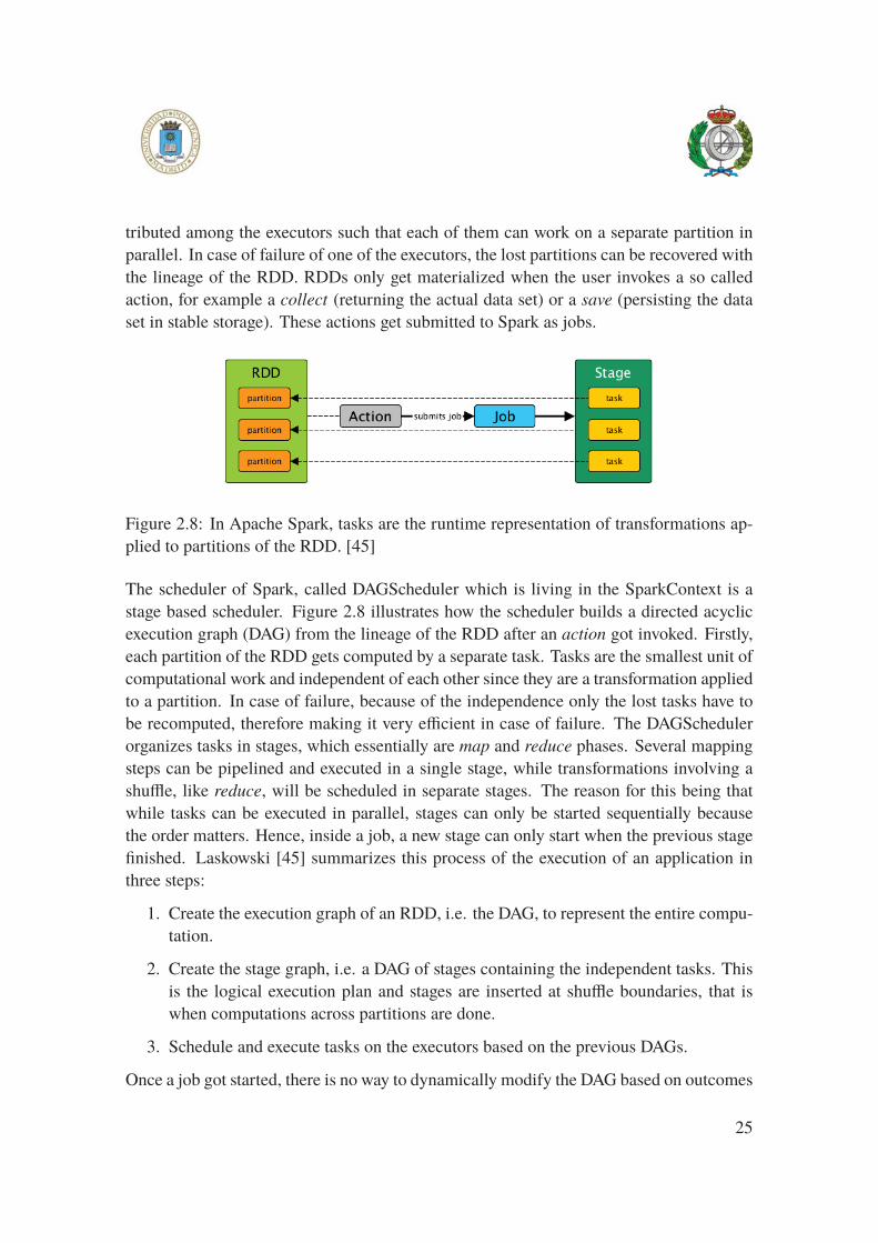
Figure 2.8: In Apache Spark, tasks are the runtime representation of transformations ap-

plied to partitions of the RDD. [45]

The scheduler of Spark, called DAGScheduler which is living in the SparkContext is a

stage based scheduler. Figure 2.8 illustrates how the scheduler builds a directed acyclic

execution graph (DAG) from the lineage of the RDD after an action got invoked. Firstly,

each partition of the RDD gets computed by a separate task. Tasks are the smallest unit of

computational work and independent of each other since they are a transformation applied

to a partition. In case of failure, because of the independence only the lost tasks have to

be recomputed, therefore making it very efficient in case of failure. The DAGScheduler

organizes tasks in stages, which essentially are map and reduce phases. Several mapping

steps can be pipelined and executed in a single stage, while transformations involving a

shuffle, like reduce, will be scheduled in separate stages. The reason for this being that

while tasks can be executed in parallel, stages can only be started sequentially because

the order matters. Hence, inside a job, a new stage can only start when the previous stage

finished. Laskowski [45] summarizes this process of the execution of an application in

three steps:

1. Create the execution graph of an RDD, i.e. the DAG, to represent the entire compu-

tation.

2. Create the stage graph, i.e. a DAG of stages containing the independent tasks. This

is the logical execution plan and stages are inserted at shuffle boundaries, that is

when computations across partitions are done.

3. Schedule and execute tasks on the executors based on the previous DAGs.

Once a job got started, there is no way to dynamically modify the DAG based on outcomes

25

of the tasks. This is an important insight for the solution proposed in this thesis. With the

stages, Spark introduces barriers in the execution of a job and one can not artificially extend

a job with additional tasks, this would need to be done in a separate job.

2.2.4 Spark and Distributed Deep Learning

In order to push the boundaries of deep learning, researchers and deep learning framework

maintainers are working on distribution strategies. These distribution strategies are meant

for training a single deep neural network on multiple machines. Deep learning requires

massive amounts of training data to achieve the best results [48] and often Spark is used to

prepare this data beforehand, therefore, increasingly more Spark users would like to embed

their distributed training in Spark applications. The challenge is, Spark and distributed

deep learning strategies do not match in their execution schemes. As outlined previously,

Spark is based on tasks which can be scheduled in an "embarrassingly parallel" fashion,

but without any communication between them. Distributed deep learning on the other

hand assume complete coordination and communication between the workers. This is

necessary, in order to propagate computed gradients and weights to all machines so that

the model can converge.

Databricks realized this mismatch and started a project called Hydrogen2 to address the

issue in Apache Spark. The first result of this project is a new scheduling mode, so called

"Gang Scheduling". Gang scheduling allows to run tasks in an "all or nothing" way, mean-

ing all tasks are started at once to block the executors, or none of them if not enough execu-

tors are available. If one of the tasks fails, the entire job fails, not making use of Sparks

failure support. The reason for these statically scheduled tasks is that now deep learn-

ing frameworks can set up communication between them in order to perform distributed

training.

2.3 Related Work

There are many frameworks tackling the challenge of hyperparameter optimization and

also Auto-ML. To name a few: On the one hand there are mainly open-source, non-

commercial solutions, of which AutoWeka [49] was the first library to include Auto-ML

techniques, auto-sklearn [50] offers an extension to the popular scikit-learn machine learn-

ing library3 or very recently auto-keras [51] gained popularity for the tuning of neural net-

2https://databricks.com/session/databricks-keynote-23More information at https://scikit-learn.org/

26

works. However, all of these have one of the following two shortcomings: 1. They do not

tackle the problem of scalability, parallelization and distribution. 2. They are compati-

ble only with a single machine learning library. On the other hand there are commercial

services: Google is providing a commercial black box optimization service in the cloud

[40], H2O.ai [52] offering an open-source platform with Auto-ML support and a com-

mercial enterprise version or determined.ai who are focusing on distributed deep learning

and hyperparameter search with their platform but aren’t open-source. Even though these

commercial offerings all tackle the scalability issue, they have the shortcoming of being

entire systems that do not integrate well into existing data processing systems and would

need to be managed and administrated, requiring additional human labour and efforts.

For the reasons above, we will not look into these solutions in more detail instead we will

look at the solution that Hopsworks was using up until now and an open-source Python

framework called Hyperopt with very similar goals to the ones we defined in section 1.3.

2.3.1 Hops-Experiments

For the past two years, the open-source Hopsworks platform has used Spark to distribute

hyperparameter optimization tasks for machine learning. Hopsworks provides some basic

optimizers (gridsearch, randomsearch, differential evolution) to propose combinations of

hyperparameters (trials) that are run synchronously over a distributed set of machines. The

implementation uses Spark as the underlying distribution engine, where trial combinations

are evaluated inside Spark map-transformations and thereby distributed over the executors.

These optimizers are contained in the experiments module of hops-util-py [53], a Python

helper library with utility functions for the Hopsworks platform.

These synchronous algorithms fit well into the Spark execution scheme. For un-directed

search a single Spark job can be started with N tasks where N is the number of trials

to be evaluated. Since RDD partitions map to Spark trials when executed, it is enough

to parallelize a local Python collection with N elements (e.g. an array [1, 2, ..., N ]) to N

partitions. Subsequently, one can call a foreachPartition with the model training function

as target function, since foreachPartition is an action, it will launch a job/stage with N

tasks. The partition itself which will be a single number can then be used inside the task

for example to select a hyperparameter combination from a array of all trials, such that

each task evaluates a different one. If the number of executors is smaller than N , Spark

will allocate the remaining tasks once slots on executors get available. When all tasks

finished, the driver collects the results and performs an aggregation to find the trial that

produced the highest or lowest accuracy/loss. The procedure is illustrated in figure 2.9 on

the left.

27

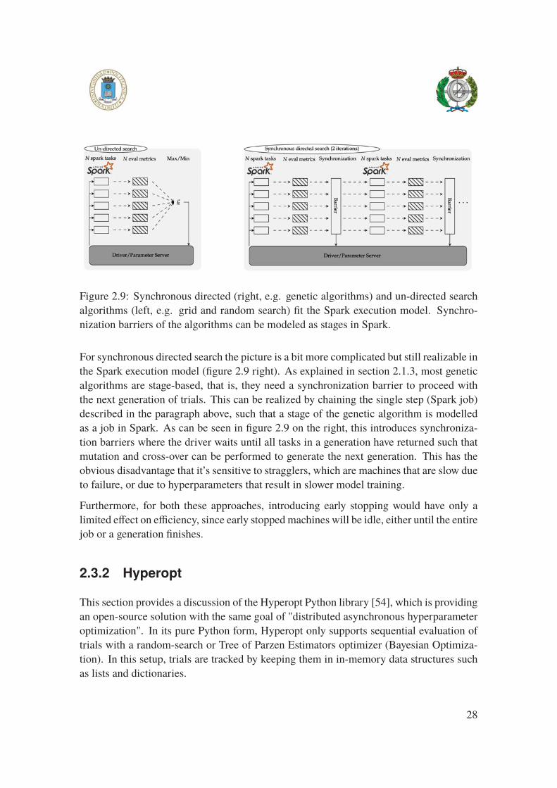
Figure 2.9: Synchronous directed (right, e.g. genetic algorithms) and un-directed search

algorithms (left, e.g. grid and random search) fit the Spark execution model. Synchro-

nization barriers of the algorithms can be modeled as stages in Spark.

For synchronous directed search the picture is a bit more complicated but still realizable in

the Spark execution model (figure 2.9 right). As explained in section 2.1.3, most genetic

algorithms are stage-based, that is, they need a synchronization barrier to proceed with

the next generation of trials. This can be realized by chaining the single step (Spark job)

described in the paragraph above, such that a stage of the genetic algorithm is modelled

as a job in Spark. As can be seen in figure 2.9 on the right, this introduces synchroniza-

tion barriers where the driver waits until all tasks in a generation have returned such that

mutation and cross-over can be performed to generate the next generation. This has the

obvious disadvantage that it’s sensitive to stragglers, which are machines that are slow due

to failure, or due to hyperparameters that result in slower model training.

Furthermore, for both these approaches, introducing early stopping would have only a

limited effect on efficiency, since early stopped machines will be idle, either until the entire

job or a generation finishes.

2.3.2 Hyperopt

This section provides a discussion of the Hyperopt Python library [54], which is providing

an open-source solution with the same goal of "distributed asynchronous hyperparameter

optimization". In its pure Python form, Hyperopt only supports sequential evaluation of

trials with a random-search or Tree of Parzen Estimators optimizer (Bayesian Optimiza-

tion). In this setup, trials are tracked by keeping them in in-memory data structures such

as lists and dictionaries.

28

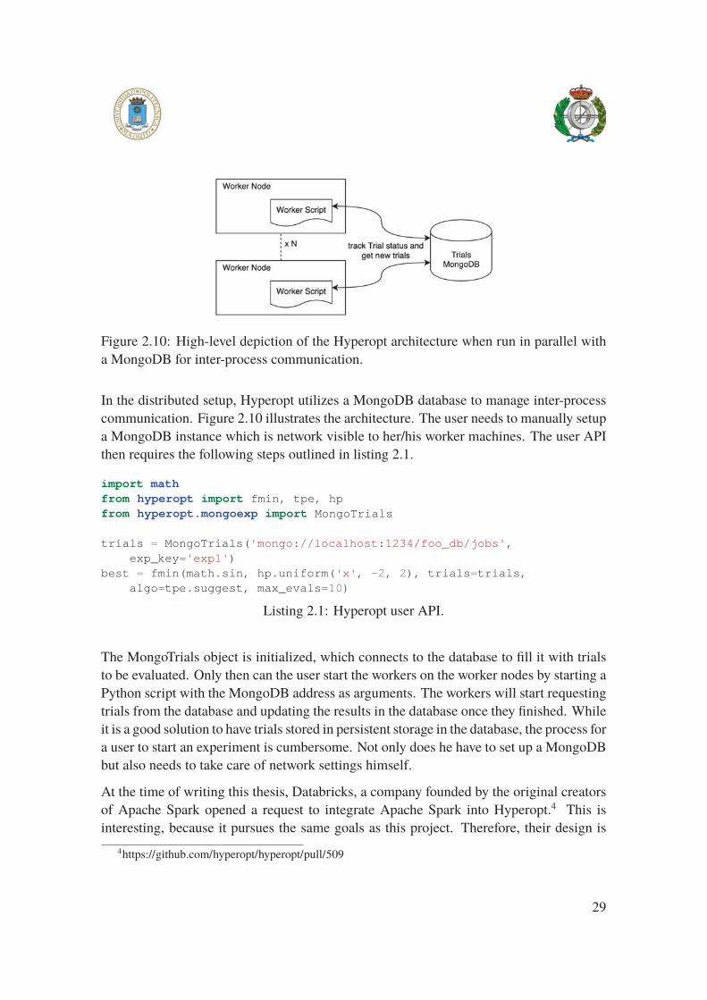
Figure 2.10: High-level depiction of the Hyperopt architecture when run in parallel with

a MongoDB for inter-process communication.

In the distributed setup, Hyperopt utilizes a MongoDB database to manage inter-process

communication. Figure 2.10 illustrates the architecture. The user needs to manually setup

a MongoDB instance which is network visible to her/his worker machines. The user API

then requires the following steps outlined in listing 2.1.

import mathfrom hyperopt import fmin, tpe, hpfrom hyperopt.mongoexp import MongoTrials

trials = MongoTrials('mongo://localhost:1234/foo_db/jobs',exp_key='exp1')

best = fmin(math.sin, hp.uniform('x', -2, 2), trials=trials,algo=tpe.suggest, max_evals=10)

Listing 2.1: Hyperopt user API.

The MongoTrials object is initialized, which connects to the database to fill it with trials

to be evaluated. Only then can the user start the workers on the worker nodes by starting a

Python script with the MongoDB address as arguments. The workers will start requesting

trials from the database and updating the results in the database once they finished. While

it is a good solution to have trials stored in persistent storage in the database, the process for

a user to start an experiment is cumbersome. Not only does he have to set up a MongoDB

but also needs to take care of network settings himself.

At the time of writing this thesis, Databricks, a company founded by the original creators

of Apache Spark opened a request to integrate Apache Spark into Hyperopt.4 This is

interesting, because it pursues the same goals as this project. Therefore, their design is

4https://github.com/hyperopt/hyperopt/pull/509

29

being outlined next with a quick note on why we rejected this design earlier before knowing

their proposal. This will become more clear in the design section later on.

In the Databricks solution, multiple threads are started on the Spark driver. Each of these

threads will submit a single job to the Spark cluster, containing a single task, which will

evaluate a single Hyperopt trial. As described in section 2.2.1, the separate threads are

necessary in order to collect the results when jobs return. These jobs with one task each

will be scheduled on arbitrary executors, similar to the Hopsworks solution in its experi-

ment module (section 2.3.1), relying on the Spark scheduler to distribute the work evenly

across the machines. We rejected this design for two major reasons:

1. Managing the job threads on the driver can become difficult. First of all, the drivers

are usually not equipped with too much computational power, so running many

threads concurrently, the driver can become a bottleneck. Secondly, to shut down

an experiment, one also needs to handle all the threads with the jobs and shut them

down gracefully since otherwise these will keep on running on the Spark cluster.

We assume these are some of the reasons why Databricks limits the number of con-

current jobs to 128.

2. This architecture does not support global early stopping decisions out-of-the-box.

The driver is unaware of the current performance of the trials that are being trained

and therefore it can not make decisions on early stopping taking all information into

account.

30

Chapter 3

Methods

3.1 Research methods

Up to this point the research methodology followed a qualitative approach, assessing pre-

vious and related work, which was needed to come up with a good design for the solution

that will be proposed in the remainder of the thesis. The research methodology in the

remainder of the thesis follows the quantitative research method.

The thesis is divided into three deliverables. The first deliverable consists of producing

a design of how asynchronous hyperparameter optimization may be integrated into the

execution model of Spark, taking into account the goals specified in section 1.3. The

second deliverable is the implementation of the software design. The final deliverable

is to conduct experiments with the produced software in order to validate if the research

hypothesis has to be rejected.

Due to time limitations, the empirical experiments conducted aim mainly at validating

the research hypothesis, that is, to prove the efficiency gains of early stopping, enabled by

the proposed solution. Asynchronous algorithms are only possible with an asynchronous

system, therefore already providing a benefit by itself. Additionally, asynchronous algo-

rithms can benefit from early stopping as an additional benefit. As a proof of concept, one

asynchronous algorithm was implemented, specifically the ASHA algorithm [44].

31

3.2 Data Collection and Analysis

Long running experiments are tracked by writing statistics to HopsFS from the Spark

driver every time a trial finishes training. The statistics include the final performance

metric of the currently best trial, the metric and training time of the recently finished trial,

the number of early stopped and total number of trials, as well as the time since the start

of the experiment. With this information, it is possible to draw conclusions on speedups

and the time it takes for optimizers to find good hyperparameter combinations.

The performance of the proposed solution itself will not be tested and benchmarked on a

lower level for the following reasons:

1. Client-server communication in the solution is not latency critical. The training of

neural networks is a computationally long process and the response times of the

server to requests by the clients are negligible in comparison. For example, if an

epoch takes 30 seconds, the server has 30 seconds to decide if the trial should be

early stopped until it gets an updated performance metric.

2. The proposed solution is highly dependent on other frameworks, and therefore, iso-

lating its performance would be tedious and influenced by the setup of Apache Spark,

for example.

3.3 Open-Source Best Practices

The software is released as open-source with the goal to create a user base that actively

contributes to the further development. To achieve this, a few best practices are adopted.

3.3.1 Semantic versioning

Versioning of the software product follows the semantic versioning1 best practices. The

version number takes the form MAJOR.MINOR.PATCH, where

• MAJOR is incremented with incompatible API changes,

• MINOR is incremented for added functionality with backwards-compatibility,

• PATCH is incremented for bug fixes with backwards-compatible bug fixes.

1Details available on https://semver.org

32

MAJOR version when you make incompatible API changes,

At the moment major version zero (0.y.z) is adopted for the software product. This is

required because anything may change at any time and the public API should not be con-

sidered stable yet by users.

3.3.2 License

The software is released under the GNU Affero General Public License v3.02. This is a

strong copy left license, requiring to disclose complete source code of licensed works and

modifications, also if it is included in larger works under the same license. The copyright

and license notices must be preserved. Contributors provide an express grant of patent

rights. When a modified version is used to provide a service over a network, the complete

source code of the modified version must be made available.

3.3.3 Documentation

Documentation of the APIs is available in a format known by most data scientists under

https://maggy.readthedocs.io/en/latest/.

2Details available on https://choosealicense.com/licenses/agpl-3.0/

33

Chapter 4

Design and Implementation

This chapter introduces the solution developed throughout the project - Maggy:1 An

open-source Python framework for asynchronous, distributed hyperparameter optimiza-

tion based on Apache Spark.23

Building on the background of the previous chapters, the first section will summarize the

motivation for such a Python library with the requirements and scenarios it should cover.

The following section describes and justifies the chosen software architecture.

4.1 Motivation and Use Case

It was shown in the background section that there are algorithms available to fulfil our

goals set in section 1.3 and the literature indicates that computational requirements of

Auto-ML and advanced HPO are a bottleneck and therefore scalability and parallelization

is desirable. So ideally, the back-box optimization loop of figure 2.3 should be adapted

to the parallelized setting illustrated in figure 4.1 to fulfil the second dimension of the

research problem defined in section 1.2. Horizontally scaling the black-box evaluations by

adding workers to evaluate a separate trial each at any time. When a worker finishes he

reports back the optimization metric to produce a new trial, which can either be kept in a

queue or directly forwarded to the idle worker.

However, this raises several challenges:

1Maggy is also a fortune teller in the television show "Game of Thrones".2Available on the Python Package Index (PyPI) and https://github.com/logicalclocks/maggy3Documentation: https://maggy.readthedocs.io/en/latest/

34

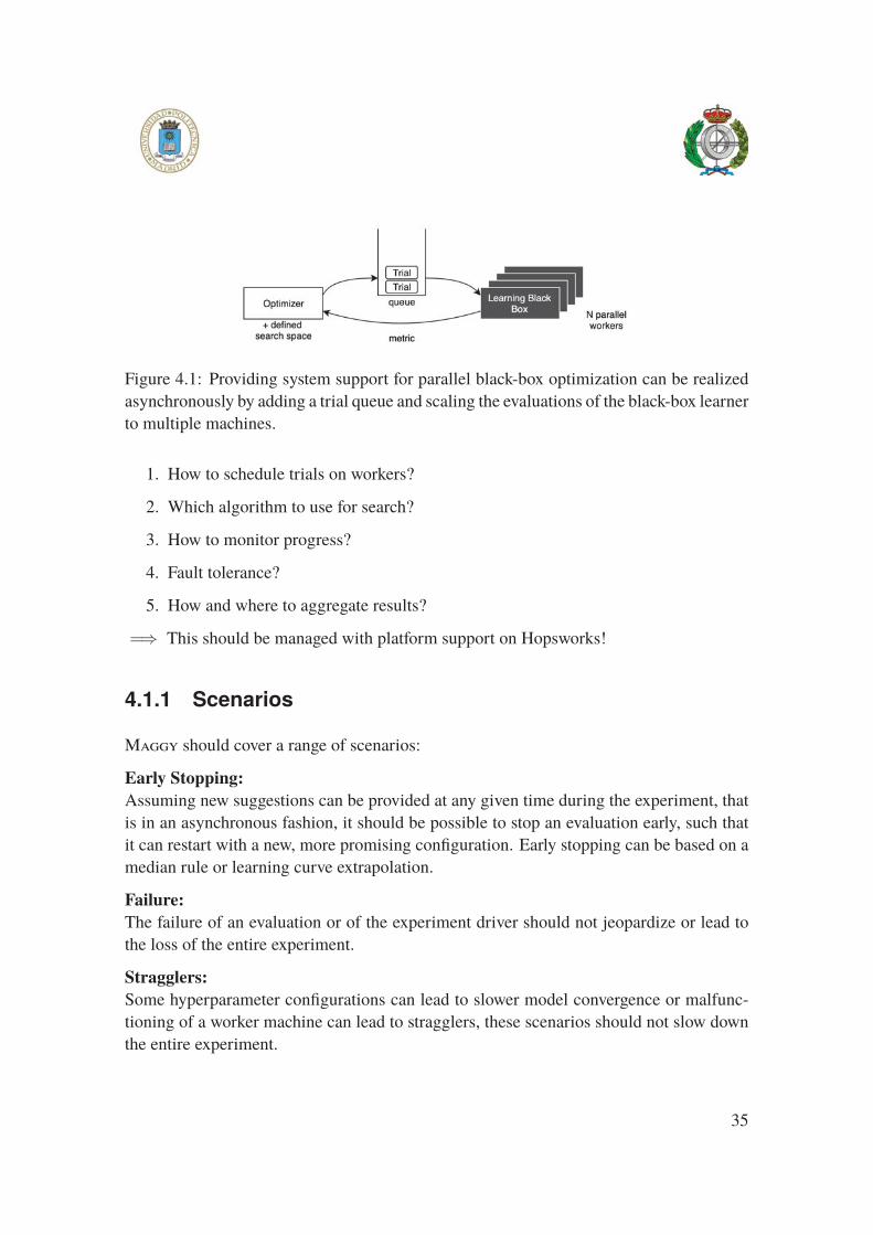
Figure 4.1: Providing system support for parallel black-box optimization can be realized

asynchronously by adding a trial queue and scaling the evaluations of the black-box learner

to multiple machines.

1. How to schedule trials on workers?

2. Which algorithm to use for search?

3. How to monitor progress?

4. Fault tolerance?

5. How and where to aggregate results?

=⇒ This should be managed with platform support on Hopsworks!

4.1.1 Scenarios

Maggy should cover a range of scenarios:

Early Stopping:Assuming new suggestions can be provided at any given time during the experiment, that

is in an asynchronous fashion, it should be possible to stop an evaluation early, such that

it can restart with a new, more promising configuration. Early stopping can be based on a

median rule or learning curve extrapolation.

Failure:The failure of an evaluation or of the experiment driver should not jeopardize or lead to

the loss of the entire experiment.

Stragglers:Some hyperparameter configurations can lead to slower model convergence or malfunc-

tioning of a worker machine can lead to stragglers, these scenarios should not slow down

the entire experiment.

35

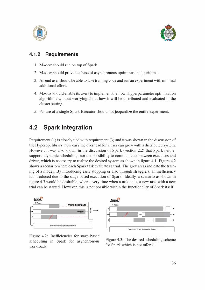
4.1.2 Requirements

1. Maggy should run on top of Spark.

2. Maggy should provide a base of asynchronous optimization algorithms.

3. An end user should be able to take training code and run an experiment with minimal

additional effort.

4. Maggy should enable its users to implement their own hyperparameter optimization

algorithms without worrying about how it will be distributed and evaluated in the

cluster setting.

5. Failure of a single Spark Executor should not jeopardize the entire experiment.

4.2 Spark integration

Requirement (1) is closely tied with requirement (3) and it was shown in the discussion of

the Hyperopt library, how easy the overhead for a user can grow with a distributed system.

However, it was also shown in the discussion of Spark (section 2.2) that Spark neither

supports dynamic scheduling, nor the possibility to communicate between executors and

driver, which is necessary to realize the desired system as shown in figure 4.1. Figure 4.2

shows a scenario where each Spark task evaluates a trial. The grey areas indicate the train-

ing of a model. By introducing early stopping or also through stragglers, an inefficiency

is introduced due to the stage based execution of Spark. Ideally, a scenario as shown in

figure 4.3 would be desirable, where every time when a task ends, a new task with a new

trial can be started. However, this is not possible within the functionality of Spark itself.

Figure 4.2: Inefficiencies for stage based

scheduling in Spark for asynchronous

workloads.

Figure 4.3: The desired scheduling scheme

for Spark which is not offered.

36

There are two possible design solutions to this challenge, the first of which was adopted by

Databricks for Hyperopt (section 2.3.2) with multiple jobs. The main disadvantage of this

design is the management of the many job threads. Instead, the design outlined in figure 4.4

was adopted. Initially, Maggy starts one task on each executor that is available to the Spark

job. These tasks are blocking the executor for the entire runtime of the HPO experiment.

Inside every task a RPC client is started, which communicates with a RPC server on the

driver (grey arrows) to get trials to evaluate and report back metrics during training for early

stopping. Additionally, both, executors and the driver can write to HopsFS (HDFS) at any

time (orange arrows), e.g. for checkpointing to persistent storage. Another advantage of

this design over the Hyperopt design is due to the RPC framework. Having a new job

per trial it would be necessary to initialize the RPC client and open a new connection to

the server every time. Each task can evaluate multiple trials sequentially, of which the

execution is controlled by the RPC client.

Figure 4.4: Maggy blocks all Spark executors with one task each and sets up communi-

cation between the tasks and the driver through an RPC framework. Both, executors and

driver can write to HopsFS (HDFS).

To allow for early stopping, the driver needs to collect current performance metrics from

each trial during training, this is realized by means of a heartbeating mechanism. The RPC

clients send a heartbeat in specified intervals with the current training metric which is to

be optimized. By collecting this information on the driver it is possible to apply globalearly stopping rules as described in section 2.1.3.

37

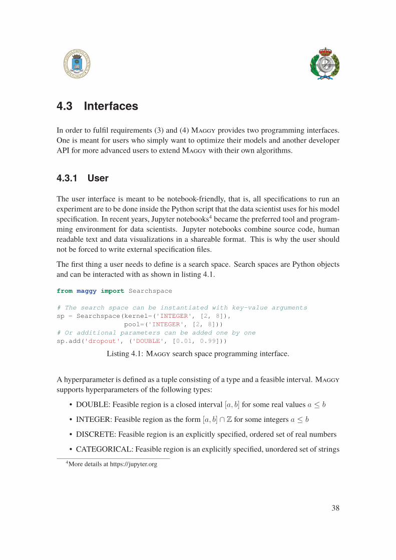
4.3 Interfaces

In order to fulfil requirements (3) and (4) Maggy provides two programming interfaces.

One is meant for users who simply want to optimize their models and another developer

API for more advanced users to extend Maggy with their own algorithms.

4.3.1 User

The user interface is meant to be notebook-friendly, that is, all specifications to run an

experiment are to be done inside the Python script that the data scientist uses for his model

specification. In recent years, Jupyter notebooks4 became the preferred tool and program-

ming environment for data scientists. Jupyter notebooks combine source code, human

readable text and data visualizations in a shareable format. This is why the user should

not be forced to write external specification files.

The first thing a user needs to define is a search space. Search spaces are Python objects

and can be interacted with as shown in listing 4.1.

from maggy import Searchspace

# The search space can be instantiated with key-value argumentssp = Searchspace(kernel=('INTEGER', [2, 8]),

pool=('INTEGER', [2, 8]))# Or additional parameters can be added one by onesp.add('dropout', ('DOUBLE', [0.01, 0.99]))

Listing 4.1: Maggy search space programming interface.

A hyperparameter is defined as a tuple consisting of a type and a feasible interval. Maggy

supports hyperparameters of the following types:

• DOUBLE: Feasible region is a closed interval [a, b] for some real values a ≤ b

• INTEGER: Feasible region as the form [a, b] ∩ Z for some integers a ≤ b

• DISCRETE: Feasible region is an explicitly specified, ordered set of real numbers

• CATEGORICAL: Feasible region is an explicitly specified, unordered set of strings

4More details at https://jupyter.org

38

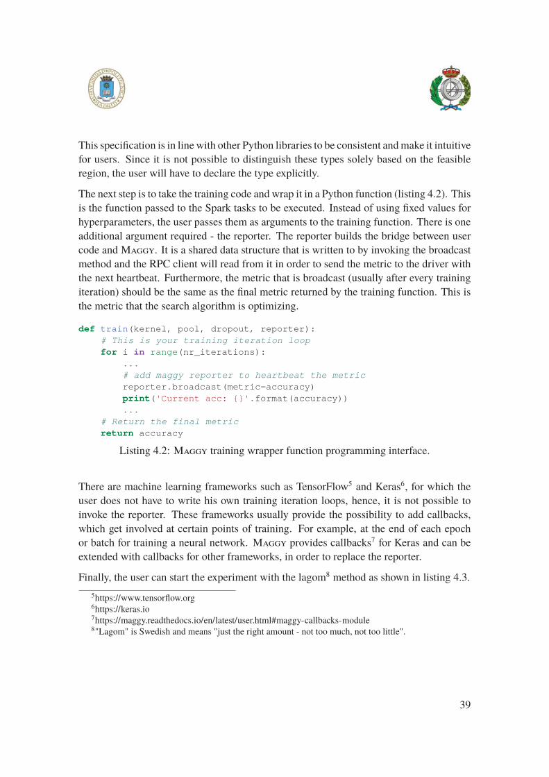
This specification is in line with other Python libraries to be consistent and make it intuitive

for users. Since it is not possible to distinguish these types solely based on the feasible

region, the user will have to declare the type explicitly.

The next step is to take the training code and wrap it in a Python function (listing 4.2). This

is the function passed to the Spark tasks to be executed. Instead of using fixed values for

hyperparameters, the user passes them as arguments to the training function. There is one

additional argument required - the reporter. The reporter builds the bridge between user

code and Maggy. It is a shared data structure that is written to by invoking the broadcast

method and the RPC client will read from it in order to send the metric to the driver with

the next heartbeat. Furthermore, the metric that is broadcast (usually after every training

iteration) should be the same as the final metric returned by the training function. This is

the metric that the search algorithm is optimizing.

def train(kernel, pool, dropout, reporter):# This is your training iteration loopfor i in range(nr_iterations):

...# add maggy reporter to heartbeat the metricreporter.broadcast(metric=accuracy)print('Current acc: {}'.format(accuracy))...

# Return the final metricreturn accuracy

Listing 4.2: Maggy training wrapper function programming interface.

There are machine learning frameworks such as TensorFlow5 and Keras6, for which the

user does not have to write his own training iteration loops, hence, it is not possible to

invoke the reporter. These frameworks usually provide the possibility to add callbacks,

which get involved at certain points of training. For example, at the end of each epoch

or batch for training a neural network. Maggy provides callbacks7 for Keras and can be

extended with callbacks for other frameworks, in order to replace the reporter.

Finally, the user can start the experiment with the lagom8 method as shown in listing 4.3.

5https://www.tensorflow.org6https://keras.io7https://maggy.readthedocs.io/en/latest/user.html#maggy-callbacks-module8"Lagom" is Swedish and means "just the right amount - not too much, not too little".

39

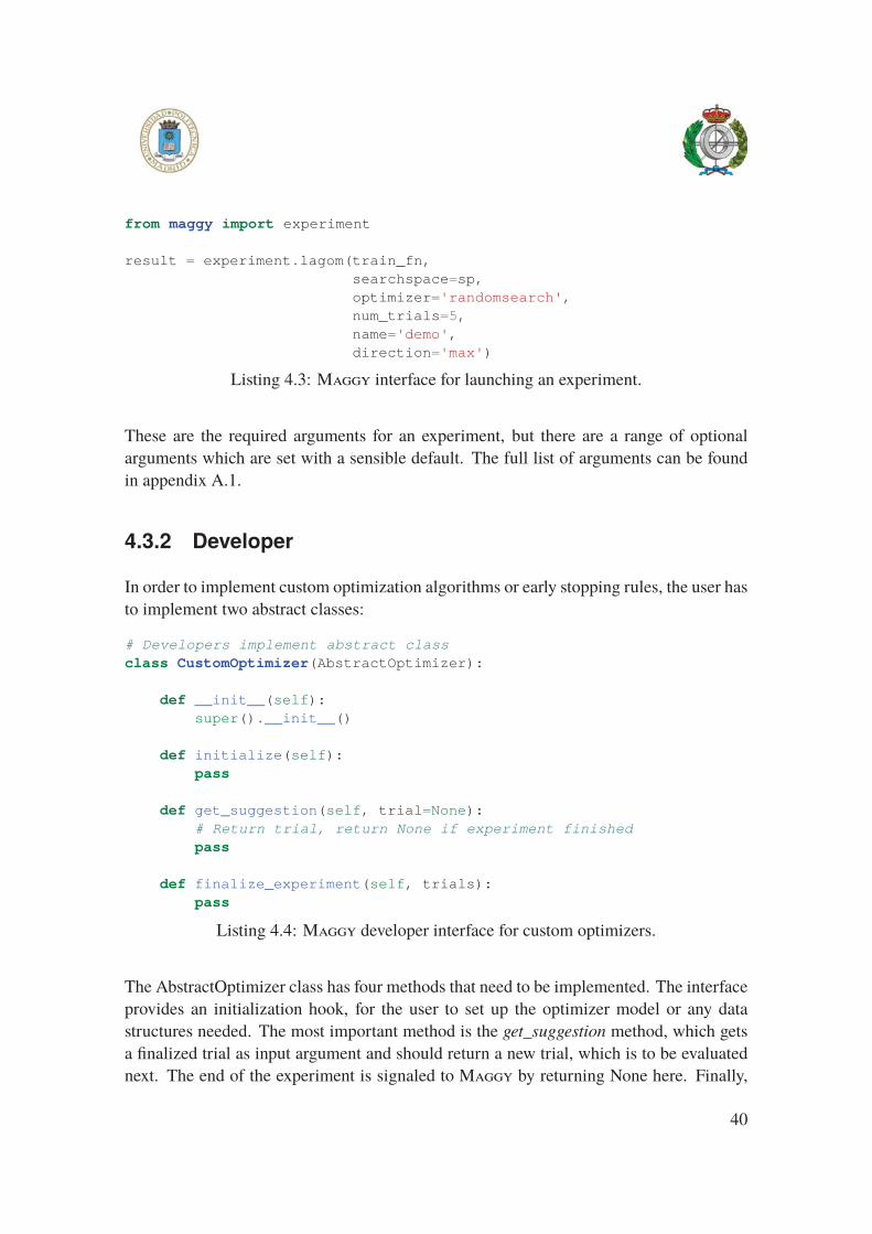
from maggy import experiment

result = experiment.lagom(train_fn,searchspace=sp,optimizer='randomsearch',num_trials=5,name='demo',direction='max')

Listing 4.3: Maggy interface for launching an experiment.

These are the required arguments for an experiment, but there are a range of optional

arguments which are set with a sensible default. The full list of arguments can be found

in appendix A.1.

4.3.2 Developer

In order to implement custom optimization algorithms or early stopping rules, the user has

to implement two abstract classes:

# Developers implement abstract classclass CustomOptimizer(AbstractOptimizer):

def __init__(self):super().__init__()

def initialize(self):pass

def get_suggestion(self, trial=None):# Return trial, return None if experiment finishedpass

def finalize_experiment(self, trials):pass

Listing 4.4: Maggy developer interface for custom optimizers.

The AbstractOptimizer class has four methods that need to be implemented. The interface

provides an initialization hook, for the user to set up the optimizer model or any data

structures needed. The most important method is the get_suggestion method, which gets

a finalized trial as input argument and should return a new trial, which is to be evaluated

next. The end of the experiment is signaled to Maggy by returning None here. Finally,

40

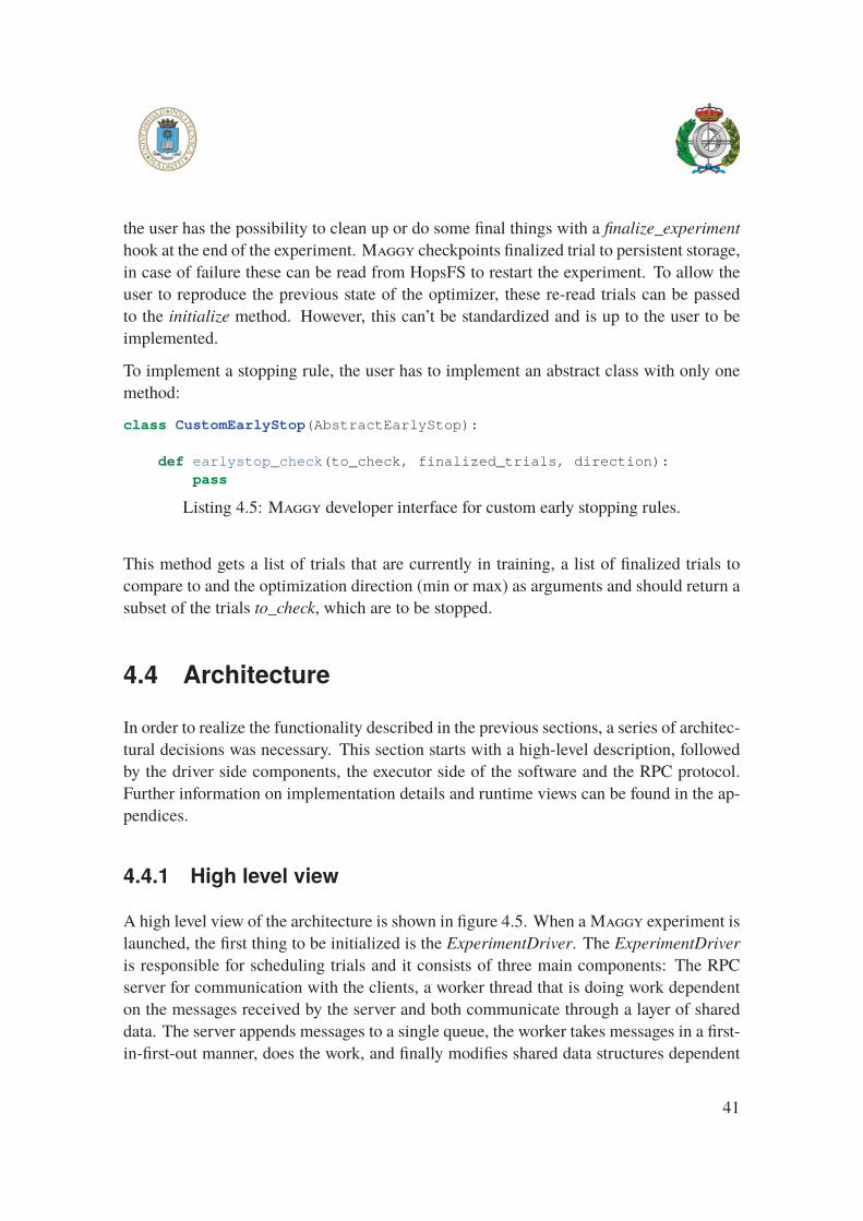
the user has the possibility to clean up or do some final things with a finalize_experimenthook at the end of the experiment. Maggy checkpoints finalized trial to persistent storage,

in case of failure these can be read from HopsFS to restart the experiment. To allow the

user to reproduce the previous state of the optimizer, these re-read trials can be passed

to the initialize method. However, this can’t be standardized and is up to the user to be

implemented.

To implement a stopping rule, the user has to implement an abstract class with only one

method:

class CustomEarlyStop(AbstractEarlyStop):

def earlystop_check(to_check, finalized_trials, direction):pass

Listing 4.5: Maggy developer interface for custom early stopping rules.

This method gets a list of trials that are currently in training, a list of finalized trials to

compare to and the optimization direction (min or max) as arguments and should return a

subset of the trials to_check, which are to be stopped.

4.4 Architecture

In order to realize the functionality described in the previous sections, a series of architec-

tural decisions was necessary. This section starts with a high-level description, followed

by the driver side components, the executor side of the software and the RPC protocol.

Further information on implementation details and runtime views can be found in the ap-

pendices.

4.4.1 High level view

A high level view of the architecture is shown in figure 4.5. When a Maggy experiment is

launched, the first thing to be initialized is the ExperimentDriver. The ExperimentDriveris responsible for scheduling trials and it consists of three main components: The RPC

server for communication with the clients, a worker thread that is doing work dependent

on the messages received by the server and both communicate through a layer of shared

data. The server appends messages to a single queue, the worker takes messages in a first-

in-first-out manner, does the work, and finally modifies shared data structures dependent

41

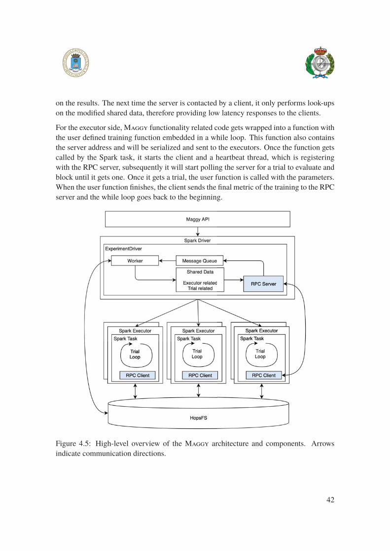
on the results. The next time the server is contacted by a client, it only performs look-ups

on the modified shared data, therefore providing low latency responses to the clients.

For the executor side, Maggy functionality related code gets wrapped into a function with

the user defined training function embedded in a while loop. This function also contains

the server address and will be serialized and sent to the executors. Once the function gets

called by the Spark task, it starts the client and a heartbeat thread, which is registering

with the RPC server, subsequently it will start polling the server for a trial to evaluate and

block until it gets one. Once it gets a trial, the user function is called with the parameters.

When the user function finishes, the client sends the final metric of the training to the RPC

server and the while loop goes back to the beginning.

Figure 4.5: High-level overview of the Maggy architecture and components. Arrows

indicate communication directions.

42

4.4.2 Driver-side

Since the Spark job blocks the main thread until it returns, the ExperimentDriver starts two

actors, the worker thread and the server listener thread. Runtime diagram A.3 in appendix

A.2 shows the main steps executed on the driver side when an experiment is set up until

the communication protocol starts.

Data structures

There are three important in-memory data structures, that the driver side actors mainly

operate on:

Reservations:The server keeps a thread safe Reservations object that is shared with the worker thread to

map Spark executors (partitions to be specific) to trial identifiers. When an executor task

registers with the server, the server creates a so called reservation for the executor which

contains information about the respective client’s host and port, partition id and trial id of

the currently scheduled trial on this executor.

Trial store:The trial store is a Python dictionary that maps trial ids to Trial objects. A Trial is a thread-

safe object to keep all information related to one trial, such as the id, the hyperparameter

configuration, status, if the trial should be stopped early, the history of the learning curve,

the final optimization metric and the start and end time of evaluation.

Final store:The final store is a simple Python list with all trials that were finalized. They are separated

from the running trials, because they need to be passed separately to certain functions,

e.g. early stopping and separating them each time would be inefficient. At the time they

are moved from the trial store to the final store, trials are also serialized and written to

HopsFS.

RPC Server

The RPC server extends a message socket class with receive and send method (appendix

figure A.2). It is implemented as a simple TCP/IP web socket server with length prefixed

pickle messages. The messages are standard Python dictionaries. The server is multi-

plexing to manage multiple client connections with a single listener thread. The server is

43

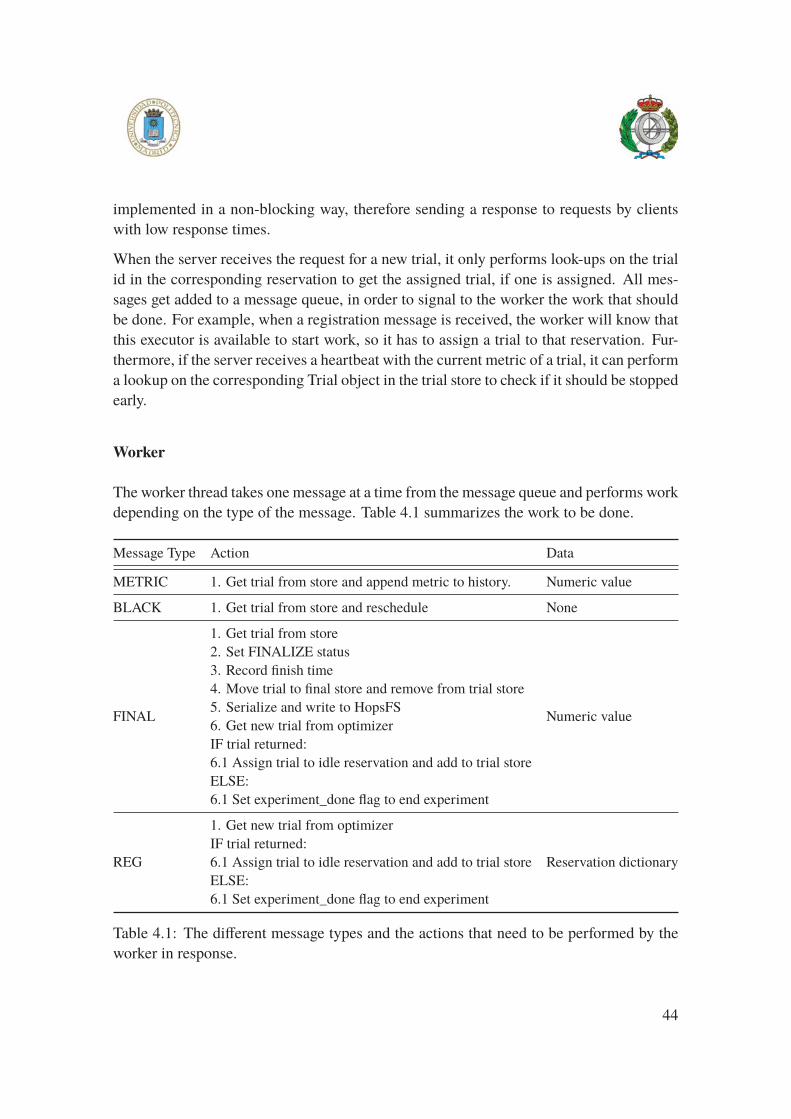
implemented in a non-blocking way, therefore sending a response to requests by clients

with low response times.

When the server receives the request for a new trial, it only performs look-ups on the trial

id in the corresponding reservation to get the assigned trial, if one is assigned. All mes-

sages get added to a message queue, in order to signal to the worker the work that should

be done. For example, when a registration message is received, the worker will know that

this executor is available to start work, so it has to assign a trial to that reservation. Fur-

thermore, if the server receives a heartbeat with the current metric of a trial, it can perform

a lookup on the corresponding Trial object in the trial store to check if it should be stopped

early.

Worker

The worker thread takes one message at a time from the message queue and performs work

depending on the type of the message. Table 4.1 summarizes the work to be done.

Message Type Action Data

METRIC 1. Get trial from store and append metric to history. Numeric value

BLACK 1. Get trial from store and reschedule None

FINAL

1. Get trial from store

2. Set FINALIZE status

3. Record finish time

4. Move trial to final store and remove from trial store

5. Serialize and write to HopsFS

6. Get new trial from optimizer

IF trial returned:

6.1 Assign trial to idle reservation and add to trial store

ELSE:

6.1 Set experiment_done flag to end experiment

Numeric value

REG

1. Get new trial from optimizer

IF trial returned:

6.1 Assign trial to idle reservation and add to trial store

ELSE:

6.1 Set experiment_done flag to end experiment

Reservation dictionary

Table 4.1: The different message types and the actions that need to be performed by the

worker in response.

44

Additionally, the worker keeps track of the time passed and checks for early stopping in

the specified early stopping interval, that is specified when launching the experiment. It

does so by calling the static method earlystop_check of the early stopping rule used in the

experiment. If the method returns trials to be stopped, the worker sets a stopping flag in the

Trial object, which will be read by the server, the next time it receives a heartbeat related

to that trial.

4.4.3 Executor-side

For the executor-side everything has to be wrapped into a function to be executed as map

function on the executors for each partition. A partition, as we mentioned earlier, is a sim-

ple integer from 0, 1, ..., N where N is the number of executors. The trialexecutor module

of Maggy contains a _prepare_func method, a higher order function, which returns the

function that is to be passed to the executors. The code snippet below shows the arguments

needed to set up the Maggy functionality inside the Spark tasks:

nodeRDD = sc.parallelize(range(num_executors), num_executors)...nodeRDD.foreachPartition(trialexecutor._prepare_func(app_id,

run_id, map_fun, server_addr, hb_interval,exp_driver._secret, app_dir))

Listing 4.6: Starting a Spark task with Maggy.

The ids are necessary in order to find the logging directories in HopsFS, map_fun is the

training function defined by the user, exp_driver._secret is a secret token to verify mes-

sages, server_addr is the host and port of the server, hb_interval is the specified interval

for the heartbeat messages and app_dir is the root directory of the application in HopsFS.

RPC Client

The RPC client implements the same message socket as the RPC server (appendix figure

A.2 for a class diagram). When the wrapper function gets called by the Spark task, the first

thing that is set up is the client. It sends a registration request with its reservation to the

server and if it was successful, the heartbeat thread is started. Subsequently, the wrapper

function enters a while loop, at the beginning of which the client starts to poll the server

for trials, either it receives a trial or it continues polling until it receives a message to end

the experiment and exit the loop.

45

Reporter

In order to send heartbeats with the current training metric to the server, the client needs

to be able to access the metric. However, the user function only returns the metric at

the very end, therefore, the reporter abstraction was introduced. The user is forced to

include the reporter in the training function signature and call reporter.broadcast(metric)in his training loop to use early stopping. The reporter is a thread-safe object, that is

written to by the user function by calling its broadcast method and the heartbeat thread

subsequently reads from it. The reporter is also responsible for early stopping the training.

When broadcast is called, it checks for a stopping flag in the reporter, if the flag is true,

the function throws a custom EarlyStopException, therefore killing the function training.

The exception is caught and the client sends the last metric to the server, notifying it that

this trial has terminated.

4.4.4 Communication

The RPC component is responsible for communication between the experiment driver

and the trial executors. A custom web socket server and client was implemented due to

the flexibility to extend the protocol. An alternative could have been the gRPC framework9, however, at the beginning the protocol was still changing frequently and gRPC requires

to generate code everytime a change is made, and hence would have been impractical for

development. Furthermore, gRPC uses Protocol Buffers10 to serialize data, which need to

be defined separately, using simple Python dictionaries was the more practical approach.

However, the replacement with the gRPC is on the future work list, because it will allow

to integrate Maggy easily with existing Hopsworks security mechanisms.

Figure 4.6 shows the communication within the system. This section focuses on the two

components on the right. When the Maggy server starts, the ExperimentDriver registers

the server address (host and port) as well as the secret token through the Hopsworks REST

API with Hopsworks. This is done, to make Maggy discoverable by other services, as

will be discussed in section 4.4.5. As mentioned before, the messages are length-prefixed

pickled dictionaries of the format shown in listing 4.7.

9https://grpc.io10https://developers.google.com/protocol-buffers/

46

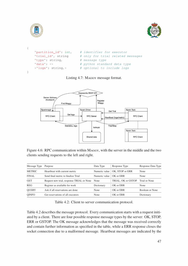
{"partition_id": int, # identifier for executor"trial_id", string # only for trial related messages"type": string, # message type"data": <> # python standard data type<"logs": string,> # optional to include logs

}

Listing 4.7: Maggy message format.

Figure 4.6: RPC communication within Maggy, with the server in the middle and the two

clients sending requests to the left and right.

Message Type Purpose Data Type Response Type Response Data Type

METRIC Heartbeat with current metric Numeric value OK, STOP or ERR None

FINAL Send final metric to finalize Trial Numeric value OK or ERR None

GET Request new trial, response TRIAL or None None TRIAL, OK or GSTOP Trial or None

REG Register as available for work Dictionary OK or ERR None

QUERY Ask if all reservations are done None OK or ERR Boolean or None

QINFO Get reservations of all executors None OK or ERR Dictionary

Table 4.2: Client to server communication protocol.

Table 4.2 describes the message protocol. Every communication starts with a request initi-

ated by a client. There are four possible response message types by the server: OK, STOP,

ERR or GSTOP. The OK message acknowledges that the message was received correctly

and contain further information as specified in the table, while a ERR response closes the

socket connection due to a malformed message. Heartbeat messages are indicated by the

47

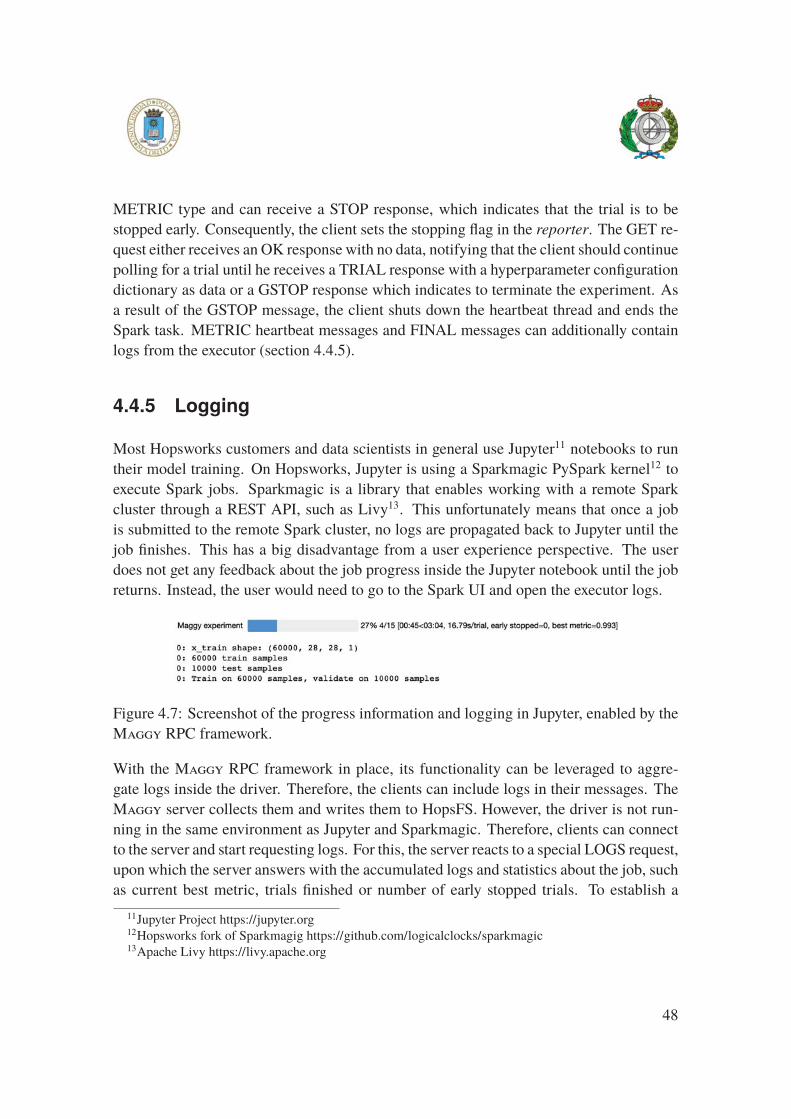
METRIC type and can receive a STOP response, which indicates that the trial is to be

stopped early. Consequently, the client sets the stopping flag in the reporter. The GET re-

quest either receives an OK response with no data, notifying that the client should continue

polling for a trial until he receives a TRIAL response with a hyperparameter configuration

dictionary as data or a GSTOP response which indicates to terminate the experiment. As

a result of the GSTOP message, the client shuts down the heartbeat thread and ends the

Spark task. METRIC heartbeat messages and FINAL messages can additionally contain

logs from the executor (section 4.4.5).

4.4.5 Logging

Most Hopsworks customers and data scientists in general use Jupyter11 notebooks to run

their model training. On Hopsworks, Jupyter is using a Sparkmagic PySpark kernel12 to

execute Spark jobs. Sparkmagic is a library that enables working with a remote Spark

cluster through a REST API, such as Livy13. This unfortunately means that once a job

is submitted to the remote Spark cluster, no logs are propagated back to Jupyter until the

job finishes. This has a big disadvantage from a user experience perspective. The user

does not get any feedback about the job progress inside the Jupyter notebook until the job

returns. Instead, the user would need to go to the Spark UI and open the executor logs.

Figure 4.7: Screenshot of the progress information and logging in Jupyter, enabled by the

Maggy RPC framework.

With the Maggy RPC framework in place, its functionality can be leveraged to aggre-

gate logs inside the driver. Therefore, the clients can include logs in their messages. The

Maggy server collects them and writes them to HopsFS. However, the driver is not run-

ning in the same environment as Jupyter and Sparkmagic. Therefore, clients can connect

to the server and start requesting logs. For this, the server reacts to a special LOGS request,

upon which the server answers with the accumulated logs and statistics about the job, such

as current best metric, trials finished or number of early stopped trials. To establish a

11Jupyter Project https://jupyter.org12Hopsworks fork of Sparkmagig https://github.com/logicalclocks/sparkmagic13Apache Livy https://livy.apache.org

48

connection to the server, the host and port are necessary. This is why the Maggy Exper-imentDriver registers the server address and the secret token with Hopsworks. A client

can then be set up within Jupyter to query logs and print them underneath the Jupyter cell.

To establish the connection, the client first requests the Maggy server information from

Hopsworks.

In order to make logging seem as pythonic as possible for the user, the Spark executors use

a special print function, that does not only print to the executor’s stderr but also tells the

client to send the content of the print to the Maggy server. In Jupyter the logs are printed

with a prefix to indicate from which executor the prints are coming. See figure 4.7 for an

example of the user experience when a Maggy experiment is run.

4.5 Failure assumptions and behaviour

4.5.1 Executor failure

In case of executor failure there are two possible scenarios:

1. Assuming that there are many executors training models simultaneously, one would

not want to stop the entire experiment and restart from a checkpoint, but rather only

restart the corrupted executor and providing it with a new suggestion as soon as it

re-registers with the experiment driver.

2. From version 2.4 Spark introduced the so called Barrier Execution Mode which is a

new scheduling strategy allowing for better failure support for distributed computa-

tions. Barrier Execution works like gang scheduling. All tasks in a barrier stage are

started at the same time. Furthermore, in this mode if one executor fails, all tasks in

the barrier stage are restarted. With this mode one would need to restore the current

state of the experiment from a checkpoint and then restart all executors.

Option number one is the more efficient option in this case and also reduces complexity,

since it is not needed to restore the entire experiment from a checkpoint. Instead, Spark

is going to restart the single task, which will register with the experiment driver again,

getting new work.

In order to guarantee this beheviour, the following Spark properties14 have to be set ac-

cordingly:

14https://spark.apache.org/docs/latest/configuration.html

49

spark.blacklist.enabled=trueBlacklisting of executors must be enabled. That means after too many task failures on an

executor, no new trials are scheduled by Spark on that executor anymore. The conditions

for blacklisting get defined with the following settings.

spark.blacklist.application.maxFailedExecutorsPerNode=2The entire node gets blacklisted for an application after two different executors got black-

listed. Since dynamic allocation is used for Maggy applications, the executors on the node

may get marked as idle and be claimed back by the cluster manager. Therefore, allowing

the application to restart new executors on the previously blacklisted node.

spark.blacklist.application.maxFailedTasksPerExecutor=1It is enough for one task to fail on an executor, for the executor to be blacklisted for the

entire application. However, the task is being attempted multiple times, as specified below.

As with blacklisted nodes, the blacklisted executor can get marked as idle and be claimed

back by the cluster manager.

spark.blacklist.stage.maxFailedExecutorsPerNode=2spark.blacklist.stage.maxFailedTasksPerExecutor=1These should be the same as the settings above on application level, since all Maggy jobs

contain only a single stage.

spark.blacklist.task.maxTaskAttemptsPerExecutor=2A specific task is being retried two times on the same executor, before the executor is black-

listed for that specific task. Because of the settings above, this also leads to a blacklisting

of the executor for the entire application.

spark.blacklist.task.maxTaskAttemptsPerNode=3A task can be retried three times on the entire node, therefore once it failed twice on one

executor, it is attempted on additional time on a different executor.

spark.blacklist.killBlacklistedExecutors=trueBlacklisted executors are being killed and reclaimed by the resource manager, such that

completely new executors can be started for the application.

spark.task.maxFailures=4Total number of failures of a particular task that are tolerated before suspending the entire

job. The total number of failures spread across different tasks will not lead to job failure.

This needs to be larger than spark.blacklist.task.maxTaskAttemptsPerNode for spark to be

robust against one unhealthy node.

spark.blacklist.timeout=60minA node or executor is unconditionally removed from the blacklist of the application after

50

one hour in order to attempt running new tasks. However, with dynamic allocation, the

executors are killed and reclaimed by the resource manager before.

With these settings, three possible reasons for failure can handled correctly:

1. Error in user code. This will lead all tasks to fail all attempts and therefore correctly

stopping the job due to the maxFailure setting.

2. Failure of executor, due to an hardware or software error outside of Maggy. The

executor will be restarted (if possible) by the Spark failure mechanisms, and subse-

quently re-registers with Maggy to get a new trial. If a trial was running at time of

failure, progress is lost, but it will be retried by Maggy either on the same executor

or a different one.

3. Failure of a trial due to a malformed hyperparameter combination. It can happen

that certain hyperparameters lead to errors because, for example, the model is to big

and the executor runs out of memory. Since trials are independent of Spark tasks,

these trials lead to the failure of the task first and hence the task restarts to get a

new trial. The trial in question will be retried either on the same or on a different

executor, however, if it fails too often, it gets discarded by Maggy itself.

4.5.2 Driver failure

Handling driver failure is not yet supported by Maggy because it always requires the user

to restart the experiment in the Jupyter notebook manually. However, the scenario was

taken into account for the design of Maggy so that the foundation is available. All finalized

trials get serialized and written to persistent storage (HopsFS) and can therefore be read

at the start of an experiment to reproduce the previous state. The finalized trials should

contain all information needed to reproduce the state of the optimizer. Alternatively the

state of the optimizer can be written to HopsFS, too, the initialize hook of the optimizer can

then be used to read the state and re-initialize. The early stopping component is stateless,

meaning it is always passed the full state of the experiment (the running and finalized

trials) to it when being called.

4.6 Security

One assumption for the security of the system is made:

51

Assumption: The user of Maggy uses Spark with encryption mode enabled, such that

tasks and jobs submitted to the executors are transferred with encryption.

The Maggy experiment driver then submits a one time secret token with the training func-

tion to the Spark executors. Due to our assumption, this token will be transferred securely.

The token will be used by the RPC clients to authenticate themselves to the Maggy exper-

iment driver. This level of security ensures that no counter party can attack the Maggy

driver with DDoS attacks, where a malicious user tries to overload a server with a large

amount of messages. The messages themselves do not contain sensitive content and are

therefore not endangering data privacy.

4.7 Testing

The testing of the system has to be split in two parts:

1. Unit tests can be performed for classes which are independent of Spark and Hops-

works, which are the Searchspace, Trial, Reporter, Optimizer and EarlyStopping-

Classes.

2. System and integration testing could be performed up to a certain point during devel-

opment, when Maggy was usable on any Spark cluster, without Hopsworks. This

was used to test the main components of the RPC framework on a Spark cluster

ran locally in standalone mode, that is, without YARN but using the internal Spark

resource manager. The test cases for this are Maggy jobs that implement certain

characteristics. Usually those are simple for loops instead of expensive model train-

ing that mimic for example certain early stopping characteristics, according to the

scenarios defined in 4.1.1. However, once Maggy was integrated with Hopsworks it

is difficult to run automated tests, because a lot of steps of running a Maggy require

interaction through the user interface and mocking all Hopsworks or Spark related

functionality would be tedious. This is a point on the future work list.

52

Chapter 5

Results and Analysis

This chapter is concerned with the third deliverable defined in section 3.1. The evaluation

of the research hypothesis. To answer this, empirical experiments were conducted. Addi-

tionally, observations about the behaviour of the system during the experiments are made,

in order to validate its functionality.

5.1 Experiments

At the time of writing, Maggy supports two optimizers, a simple random-search approach

[29] and the adaptive configuration selection algorithm ASHA [44]. Additionally, the me-

dian stopping rule was implemented for early stopping. Random-search is used in con-

junction with the median stopping rule to validate the research hypothesis on two tasks:

1. Hyperparameter optimization of a convolutional neural network (CNN) for image clas-

sification. 2. A small CNN architecture search task. Additionally, ASHA is compared to

random-search with early stopping on these two tasks, in order to investigate if the directed

nature of ASHA yields benefits over the un-directed random-search, but with additional

early stopping.

53

5.1.1 Experimental Setup

Data

The CIFAR-10 dataset [55] was used throughout all experiments. The dataset consists of

60,000 32x32 colour images with 10 classes, with 6,000 images per class. And it is split

into 50,000 training images and 10,000 validation images. This is a common dataset and

is widely used in research and in most Auto-ML related articles that were presented in the

background section, e.g. [8] [33] [44] [43]. A test set for the final evaluation of the model

is not used since a test set should never be used for hyperparameter tuning. This dataset

poses a high enough computational challenge because it requires deep neural networks to

achieve good accuracies.

Environment

The experiments are run on a single node Google Cloud instance with 68GB memory, 22

vCores and 4 NVIDIA Tesla P100 GPUs with 16GB memory each. The node is running

Hopsworks 0.10.0 with Apache Spark 2.4.0.1 and Maggy 0.2.2. Therefore, experiments

can be run with four concurrent workers/executors with one vCore and with one GPU each.

Each executor and also the driver gets allocated 8GB of memory. The neural networks are

implemented with the Keras API of TensorFlow version 1.11.01.

To make results comparable, for each of the following three experiments, a maximum

compute time on the four executors was set as a resource. That means, per experiment

each searcher was run for a limited time. The time was determined by running first the

ASHA optimizer and subsequently running random-search with and without early stop-

ping for the same amount of time. Since the optimizers are based on randomness, each

of the experiments is rerun three times and the averages are reported. Due to the high

computational cost of these experiments, especially the GPUs, more repititions were not

possible. However, this shows once again how important efficient optimization techniques

are.

5.1.2 Hyperparameter Optimization Task

The first experiment conducted is a hyperparameter tuning task. The experimental design

of Li et al. [8] for CIFAR-10 was used, which they adopted from Snoek, Larochelle, and

1https://www.tensorflow.org/versions/r1.11/api_docs/python/tf/keras

54

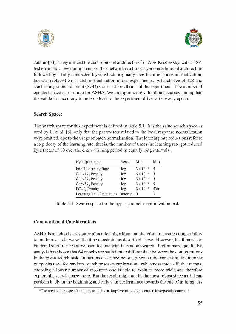
Adams [33]. They utilized the cuda-convnet architecture 2 of Alex Krizhevsky, with a 18%

test error and a few minor changes. The network is a three-layer convolutional architecture

followed by a fully connected layer, which originally uses local response normalization,

but was replaced with batch normalization in our experiments. A batch size of 128 and

stochastic gradient descent (SGD) was used for all runs of the experiment. The number of

epochs is used as resource for ASHA. We are optimizing validation accuracy and update

the validation accuracy to be broadcast to the experiment driver after every epoch.

Search Space:

The search space for this experiment is defined in table 5.1. It is the same search space as

used by Li et al. [8], only that the parameters related to the local response normalization

were omitted, due to the usage of batch normalization. The learning rate reductions refer to

a step decay of the learning rate, that is, the number of times the learning rate got reduced

by a factor of 10 over the entire training period in equally long intervals.

Hyperparameter Scale Min Max

Initial Learning Rate log 5 ∗ 10−5 5

Conv1 l2 Penalty log 5 ∗ 10−5 5

Conv2 l2 Penalty log 5 ∗ 10−5 5

Conv3 l2 Penalty log 5 ∗ 10−5 5

FC4 l2 Penalty log 5 ∗ 10−3 500

Learning Rate Reductions integer 0 3

Table 5.1: Search space for the hyperparameter optimization task.

Computational Considerations

ASHA is an adaptive resource allocation algorithm and therefore to ensure comparability

to random-search, we set the time constraint as described above. However, it still needs to

be decided on the resource used for one trial in random-search. Preliminary, qualitative

analysis has shown that 64 epochs are sufficient to differentiate between the configurations

in the given search task. In fact, as described before, given a time constraint, the number

of epochs used for random-search poses an exploration - robustness trade-off, that means,

choosing a lower number of resources one is able to evaluate more trials and therefore

explore the search space more. But the result might not be the most robust since a trial can

perform badly in the beginning and only gain performance towards the end of training. As

2The architecture specification is available at https://code.google.com/archive/p/cuda-convnet/

55

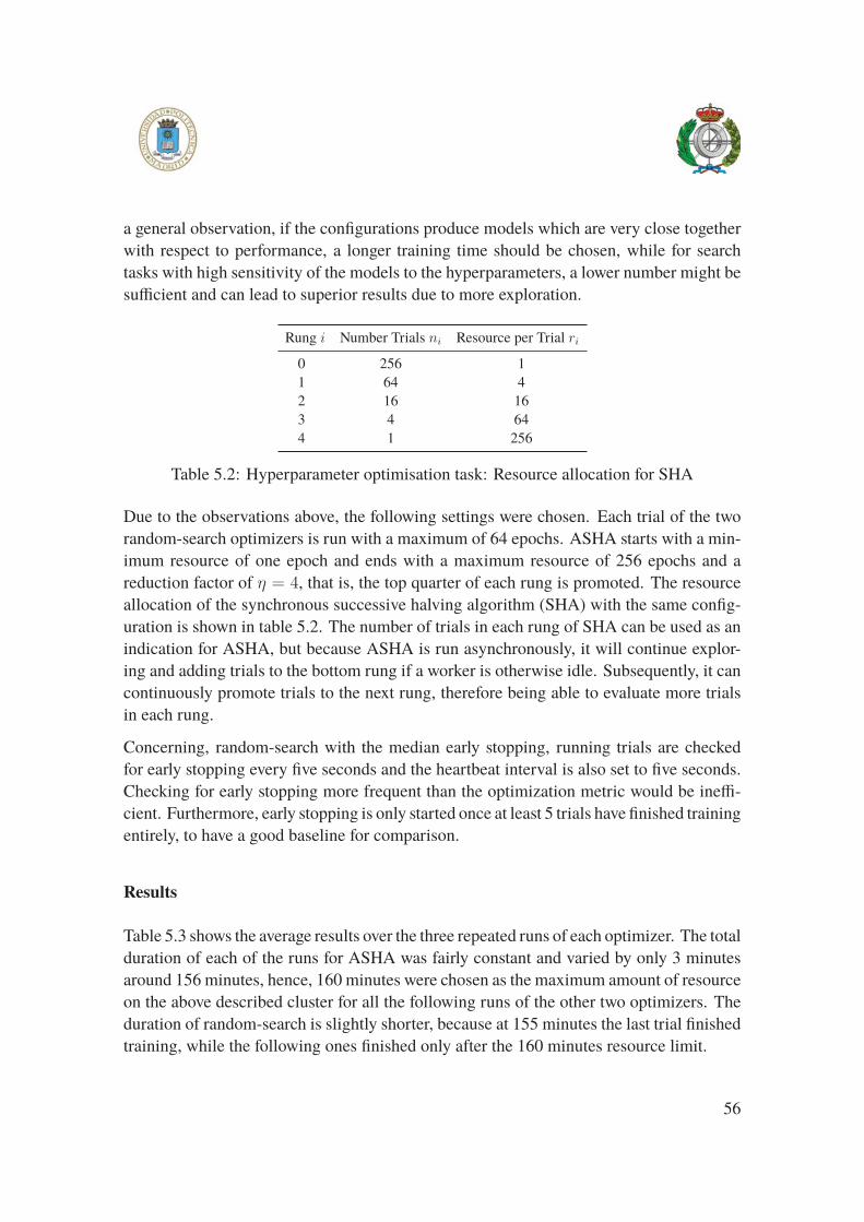
a general observation, if the configurations produce models which are very close together

with respect to performance, a longer training time should be chosen, while for search

tasks with high sensitivity of the models to the hyperparameters, a lower number might be

sufficient and can lead to superior results due to more exploration.

Rung i Number Trials ni Resource per Trial ri

0 256 1

1 64 4

2 16 16

3 4 64

4 1 256

Table 5.2: Hyperparameter optimisation task: Resource allocation for SHA

Due to the observations above, the following settings were chosen. Each trial of the two

random-search optimizers is run with a maximum of 64 epochs. ASHA starts with a min-

imum resource of one epoch and ends with a maximum resource of 256 epochs and a

reduction factor of η = 4, that is, the top quarter of each rung is promoted. The resource

allocation of the synchronous successive halving algorithm (SHA) with the same config-

uration is shown in table 5.2. The number of trials in each rung of SHA can be used as an

indication for ASHA, but because ASHA is run asynchronously, it will continue explor-

ing and adding trials to the bottom rung if a worker is otherwise idle. Subsequently, it can

continuously promote trials to the next rung, therefore being able to evaluate more trials

in each rung.

Concerning, random-search with the median early stopping, running trials are checked

for early stopping every five seconds and the heartbeat interval is also set to five seconds.

Checking for early stopping more frequent than the optimization metric would be ineffi-

cient. Furthermore, early stopping is only started once at least 5 trials have finished training

entirely, to have a good baseline for comparison.

Results

Table 5.3 shows the average results over the three repeated runs of each optimizer. The total

duration of each of the runs for ASHA was fairly constant and varied by only 3 minutes

around 156 minutes, hence, 160 minutes were chosen as the maximum amount of resource

on the above described cluster for all the following runs of the other two optimizers. The

duration of random-search is slightly shorter, because at 155 minutes the last trial finished

training, while the following ones finished only after the 160 minutes resource limit.

56

At the end of the entire runtime of the experiment, ASHA returned best performing hy-

perparameter configurations with an average accuracy of 81.36%. Which is comparable

to the model found by the Hyperband method of Li et al. [8], who report an approximate

accuracy of 21%. However, they only report the results in relation to epochs trained and

not in relation to time, which can vary depending on the infrastructure used. Nevertheless,

it can be seen that both asynchronous methods, ASHA and random-search with the me-

dian stopping rule (RS-ES) find competitive configurations. Only random-search without

early stopping (RS-NS) cannot find a competitive configuration with an average accuracy

of 77.5%.

The previous observation is not surprising, looking at the number of trials that were con-

sidered by each of the methods, RS-NS trained only 36 models, however, each of them

for 64 epochs. On the other hand, ASHA considered 442 trials with an average duration

of only about one minute. It should be noted that ASHA did not early stop trials, but

instead has the adaptive resource allocation. Surprisingly, all three runs of ASHA evalu-

ated exactly the same number of trials and took about the same time. The same holds for

RS-NS, which was able to evaluate 36 trials in all three runs. One would have expected

that different hyperparameter configurations lead to varying training speeds. However, it

could be seen that due to the simplicity and small size of the neural network in compari-

son to the high computational power of the GPUs, every epoch took about the same time.

That means, training time was independent of the configuration and only dependent on

the amount of data, which was the same in all three runs. Monitoring the GPU utilization

during the experiments substantiated this observation, as the GPUs barely got over 30%

utilization.

Table 5.2 shows that synchronous successive halving would have considered only 346

trials, ASHA improved over that with 442, that is an increase of about 27% even with

only four workers - an effect that will be amplified with more workers. RS-ES considered

on average 120 trials, of which on average 90 were stopped early, with large standard

deviations across the three runs. This poses a considerable speedup with respect to the

amount of trials considered, that is the exploration of the search space. It can be seen from

the large standard deviation of the duration of the trials in RS-ES that most trials were

stopped very early in the training process, thus, being in line with our hypothesis. Overall,

the large variance in the duration of trials in the asynchronous algorithms together with

the superior performance justifies the need for platform support of asynchronous HPO

algorithms.

Figure 5.1 shows the average accuracies tracked over the runtime of the experiment. It

can be seen that ASHA finds good configurations already early during the experiment,

showing its superiority and the importance of exploration of the search space. The vertical

57

Optimizer Runs Total Duration Best Accuracy (Std) Trials (Std) Trials Stopped (Std) Trial Duration (Std)

ASHA 3 156 0.8136 (0.02) 442 (0.0) 0 (0.0) 0.98 (3.53)

Random-search with

Median Stopping (RS-ES)3 160 0.7958 (0.01) 120 (60.7) 90 (65.3) 5.18 (7.28)

Random-search with

No Stopping (RS-NS)3 155 0.7747 (0.04) 36 (0.0) 0 (0.0) 17.22 (0.04)

Table 5.3: Hyperparameter optimization task: Average results over three repeated runs per

optimizer with standard deviations in parentheses.

line indicates the point when ASHA decided on it’s final configuration. The larger gaps

in accuracy at this point between the methods make its superiority more clear. From that

point on it only trains the single last model with 256 epochs. So actually, it finds the best

configuration already after 76 minutes and therefore achieves a 2x speedup to the other

two methods. In fact, ASHA finds the best configuration and returns a fully trained (256

epochs) model, while the other two return only models trained for 64 epochs and would

need another 256 epochs to train the full best model.

Figure 5.1: Hyperparameter optimization task: Average best accuracy over three repeated

runs per optimizer tracked over the runtime of the experiment with the cuda-convnet ar-

chitecture.

Comparing RS-ES and RS-NS it should be noted, that RS-NS finds better configurations

early in the experiment. This could be an indicator, that the early stopping method actually

stops some configurations which might have improved their accuracy rather late during

the training process. However, as noted before, RS-NS fails to find a overall competitive

configuration. We extended the duration of RS-NS and found that it finds competitive

configurations only after around twice the amount of time, so more than five hours.

58

5.1.3 Neural Architecture Search Task

To pose a computationally more challenging task, the second experiment conducted was

a neural architecture search task. We are tuning the architecture of a small convolutional

neural network. For that an approach is adopted, that is also adopted for state-of-the-art

NAS: Data scientists define a micro architecture of so called "cells" and subsequently the

architecture is tuned by finding the number of cells in sequence and tuning the hyper-

parameters of the cell. The search space is defined in detail below. As in the previous

experiment, a batch size of 128 and SGD was used for all runs and the number of epochs

is used as resource for ASHA. The validation accuracy is updated and broadcast to the

experiment driver after every epoch for early stopping and optimization.

Search Space

The network consists of at least one and maximum three sequential convolutional cells,

followed by one last fully connected layer and dropout before the soft-max output layer.

Except for the output and the pooling layers, all layers use a rectified linear unit (ReLU) as

activation function. The number of neurons in the fully connected layer is made a hyper-

parameter as well as the dropout rate applied to it. The convolutional cells are structured

beginning with one to three sequential convolutional layers, followed by either a maximum

or average pooling layer. The number of filters in the convolutional layers is a hyperpa-

rameter, and if there is more than one cell, the last cell will have double the amount of

filters. Finally, to each cell dropout is applied. There are two more overall hyperparame-

ters, that are the initial learning rate and a constant decay factor. This experiment design

was in part adapted from the "small CNN architecture tuning task" of Li et al. [44], how-

ever, there specification is not complete. A discussion of the original ASHA experiment

can be found in the appendix. The feasible intervals and values for the hyperparameters

are shown in table 5.4.

Computational Considerations

The same resource allocation per trial as in the previous experiment is used for all opti-

mizers. Furthermore, also the settings for early stopping are the same.

59

Hyperparameter Scale Min Max

Initial Learning Rate log 10−5 1

Learning Rate Decay log 10−7 10−3

Number Conv. Cells integer 1 3

Number Conv. Layers/Cell integer 1 3

Number of Filters discrete {16, 32, 48, 64}Pooling categorical {avg,max}Cell Dropout Rate real 10−3 0.9

Neurons Fully Connected discrete {64, 128, 256, 512, 1024}Dropout Rate Fully Connected real 10−3 0.9

Table 5.4: Search space for the neural architecture search task.

Results

The overall results for the neural architecture search task are summarized in table 5.5.

The first observation that can be made, are the overall high accuracies above 80% for all

three optimizer. This indicates that all the models perform well and are not as sensitive to

the hyperparameter configurations, as the cuda-convnet model in the previous experiment.

Convolutional neural networks with pooling layers and dropout are known to perform well

on image recognition tasks and CIFAR-10 is not the most complex learning task. More-

over, the structure of the previously defined architecture cells are a common approach and

therefore the good performance is not surprising. However, this makes the task about find-

ing small deviations in architecture that are hard to be discovered by humans. The good

quality of the models gets apparent, too, when we look at the standard deviation of the

amount of early stopped trials. The standard deviation is here only 13.86 compared to

65.3 in the previous task. Hence, the median rule is consistently stopping between 70%

and 90% trials, indicating more stable model performances. Because of the fewer stopped

trials, RS-ES can evaluate only 107 trials. Interestingly, ASHA is still able to evaluate

441 trials, only one less than before, indicating that even though the NAS models’ archi-

tectures are larger in terms of parameters to be learned, the computational complexity of

the training is still not having an impact on the training time per trial. The GPUs are fast

enough to cover the variances in architecture size.

Figure 5.2 plot the average accuracies of the best performing configurations over time.

The four workers in the two random-search approaches each finalize the first set of trials

after 17 minutes, and the four models already have an average performance of 74% for

both approaches, this confirms again that model accuracy is overall high on the given task.

Again the grey vertical line indicates the point until ASHA trained no model with more

than 64 epochs. The training of the final model of ASHA with 256 epochs took about 70

60

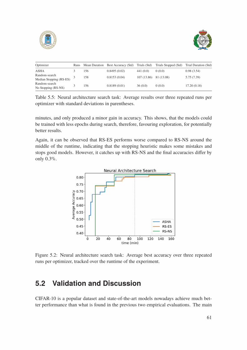
Optimizer Runs Mean Duration Best Accuracy (Std) Trials (Std) Trials Stopped (Std) Trial Duration (Std)

ASHA 3 156 0.8495 (0.02) 441 (0.0) 0 (0.0) 0.98 (3.54)

Random-search

Median Stopping (RS-ES)3 158 0.8153 (0.04) 107 (13.86) 81 (13.08) 5.75 (7.39)

Random-search

No Stopping (RS-NS)3 156 0.8189 (0.01) 36 (0.0) 0 (0.0) 17.20 (0.18)

Table 5.5: Neural architecture search task: Average results over three repeated runs per

optimizer with standard deviations in parentheses.

minutes, and only produced a minor gain in accuracy. This shows, that the models could

be trained with less epochs during search, therefore, favouring exploration, for potentially

better results.

Again, it can be observed that RS-ES performs worse compared to RS-NS around the

middle of the runtime, indicating that the stopping heuristic makes some mistakes and

stops good models. However, it catches up with RS-NS and the final accuracies differ by

only 0.3%.

Figure 5.2: Neural architecture search task: Average best accuracy over three repeated

runs per optimizer, tracked over the runtime of the experiment.

5.2 Validation and Discussion

CIFAR-10 is a popular dataset and state-of-the-art models nowadays achieve much bet-

ter performance than what is found in the previous two empirical evaluations. The main

61

difference in performance attributable to more complex models with deeper architectures

and data manipulation to artificially increase the size of the dataset. Li et al. [8] argue,

that if you limit the comparison to the best human expert result and the same architecture

(cuda-convnet), the best test error is 18% and optimized 15% [33]. Considering, that we

used a slightly altered search space and architecture with batch normalization, the results

are reasonable. One has to note, too, that the experiments were also conducted with less

resources. Li et al. [8] train their models for 75 epochs.

It was observed multiple times in the results above, that the duration of trials seems to

be deterministic because ASHA and random-search without early stopping consistently

evaluated the same amount of trials across the three repetitions of the search. We gave

a possible explanation for this phenomenon, that due to the computational power of the

GPUs, the training time is independent of the hyperparameter configuration or architec-

ture. A first suspicion was, that the process might not be truly random, but sanity checks

were conducted to ensure that configurations are sampled randomly from the search space.

At no point were random seeds being set during the experiments. For an example, where

the hyperparamter configurations influence training time, the reader is being refered to the

additional experiment in appendix B.1.

System Design

The constant run times, mentioned in the paragraph, above approve the design of the

Maggy architecture. The Maggy server can easily handle heartbeats with one second

intervals from multiple workers and does not slow down the trials due to the non blocking

communication protocol.

During the execution of very long experiments, an issue with the GPUs occurred. The

GPUs were causing out-of-memory exceptions in an undeterministic manner. The prob-

lem was in the memory allocation on the GPU by TensorFlow. By default, TensorFlow

claims almost all memory on GPUs, in order to reduce issues with memory fragmen-

tation3. The memory allocation only gets released when the host Python process, that

started the TensorFlow backend, gets stopped. Since we are training models in serial from

the same Python process, TensorFlow was accumulating garbage on the GPUs’ memory,

eventually causing the out-of-memory errors. This happened despite the small size of the

models. There were two remedies to this issue. The first would be a hard reset of the

GPUs’ memory by a subprocess through the NVIDIA System Management Interface4,

3More details at https://www.tensorflow.org/guide/using_gpu#allowing_gpu_memory_growth4More details at https://developer.nvidia.com/nvidia-system-management-interface

62

which provides a command line interface to the management of NVIDIA GPUs. The sec-

ond possibility was to close the TensorFlow session and to reset the TensorFlow default

graph subsequently. The second option allows to finally perform garbage collection. Since

Hopsworks provides support for AMD GPUs, the first option was not universal, because it

is specific to NVIDIA. Hence, the second option was chosen. The process of doing these

operations can be hidden from the user by placing them in the RPC client of Maggy,

calling them before every new trial.

It was described in section 4.4, that Maggy keeps the state of all trials in memory through-

out the runtime of an experiment even though it writes them to HopsFS. This could become

a problem memory bottleneck on the Spark driver for long experiments with many trials.

For that reason, it was tried to estimate the size of the state of a trial. It is known, that

it is not straight forward to determine the in-memory size of a custom Python object5.

One of the reasons for that being that Python works with references to other objects inside

Python standard objects like lists or dictionaries. Furthermore, lists for example always

reserve more space in memory than necessary. As a quick estimate, an approach was cho-

sen that gets often proposed for Python. For that the object simply gets pickled, that is,

serialized and subsequently the length of pickle object is measured. It was found that for

the experiments conducted, the trials varied from a size of 0.3KB to 0.6KB, depending on

the length of the history for the learning curve. This shows that the trial size should not

become an issue, which could also be seen when the memory consumption on the driver

was monitored during experiments.

5For more details:

https://stackoverflow.com/questions/33978/find-out-how-much-memory-is-being-used-by-an-object-in-python

63

Chapter 6

Conclusion

Coming back to the problem description introduced in section 1.2, the first identified

problem was the algorithmic side of hyperparameter optimization. The literature review

showed, that asynchronous algorithms exist, for example Bayesian Optimization, ASHA

or Hyperband. Furthermore, methods to increase performance evaluation efficiency such

as early stopping can additionally be used to create additional asynchronism, measured in

the variance in trial duration. The literature suggests that directed algorithms outperform

un-directed approaches such as random and grid-search on most learning tasks. Moreover,

state-of-the-art algorithms such as ASHA can often be operated asynchronously, therefore,

substantiating our claim that there is a need for system support of asynchronous optimiza-

tion methods.

This brings us to the second dimension of the problem. Apache Spark is widely adopted

and to avoid additional administration overhead for a new system, we wanted to be able to

leverage the scheduling and fault-tolerance capabilities of Spark. However, Spark’s execu-

tion model is inherently synchronous and constrained by limited possibilities for commu-

nication between worker nodes. Especially for distributed deep learning, this poses a mis-

match, because complete coordination and communication between executors is needed.

We circumvented this shortcoming with a light-weight RPC framework and we have shown

that it is possible to implement a scalable, asynchronous, distributed system for hyperpa-

rameter optimization in this way, based on Apache Spark. We decided to release this

project as open-source, in order to allow users to implement their own algorithms and

hopefully become active contributors to the project. There are many open-source solu-

tions that try to solve the same or similar problems, however, fail to fulfil at least one of

the goals defined in section 1.3. We have shown this on the example of Hyperopt, which

has the same goal as Maggy, but fails to provide a user friendly API for distributed exper-

64

iments. It will be interesting to see, how the Hyperopt Spark integration will be adopted

by the community and if Maggy can compete with it.

To summarize the benefits of Maggy, we can conclude that Maggy not only fulfils the

defined goals, but provides:

• Support for asynchronous optimization algorithms (random-search, ASHA)

• Support for early stopping

• Robustness against stragglers

• Simple, notebook friendly and extendable API

Additionally, if Maggy is run on Hopsworks with underlying HopsFS as persistent storage,

Maggy provides:

• Fault tolerance with checkpointing of experiment state

• Log aggregation and realtime prints in Jupyter

• Monitoring with TensorBoard (HParams plugin, introduction with TensorFlow ver-

sion 2.0)

Finally, we can accept the research hypotheses. ASHA, as a state-of-the-art asynchronous

algorithm with its builtin principled early stopping capabilities, consistently outperforms

un-directed approaches without early stopping, that is random-search. A lot of research ar-

gues that on most learning tasks random-search is a baseline that is hard to beat [11] and in-

deed it is. Adding an early stopping rule such as the median stopping rule to random-search

only increases the efficiency on specific learning tasks. Those tasks are the ones where the

models are sensitive to hyperparameter combinations. For models which perform gener-

ally well, as we have shown in the NAS task, early stopping brings only limited benefits.

However, it should be noted that the performance of these methods is greatly influenced

by the resource allocated to the training of each model. By setting this resource, the expert

can trade-off between exploration and the robustness of results. Generally, this depends

on the resources required for the trials to sufficiently differentiate themselves in terms of

generalization error. That is, if randomly selected hyperparameter combinations possess

similar performance or when models converge slowly then one should work with larger per

trial resources. On the other hand, if the generalization capability is revealed early during

training, minimal resources per trial make sense in order to favour exploration. This obser-

vation is in accordance with the findings of Li et al. [8] for their Hyperband method, who

conclude that the most explorative bracket of Hyperband is preferable in high-dimensional

spaces and fast converging training procedures. Principled early stopping techniques such

as ASHA avoid this "new" hyperparameter, therefore, giving it another advantage.

65

6.1 Future Work

Maggy is an open-source project and we will continue on extending and improving it.

The future work to be done on Maggy should include:

1. Implementation of more optimizers and stopping rules such as Bayesian Optimiza-

tion and learning curve prediction. In order to be competitive and generate a larger

user base, more algorithms will be implemented for Maggy.

2. Fault-tolerance and warm starting of experiments. The state of the experiment is

being checkpointed to persistent storage, however, since restarting an experiment is

dependent on the initialization of the optimizer, there is still work to be done.

3. In principle Maggy can be used with any machine learning library. However, there

might occur unforeseen issues, such as the TensorFlow GPU problem described ear-

lier. It is planned to add tested support for PyTorch1 to Maggy.

4. Implement a standardized way of testing for Maggy. Due to its integration in exist-

ing systems, testing of Maggy is challenging and except for unit tests relies on test

experiments at the moment. There should be a way to test Maggy in a simpler more

standardized way. One way could be the setup of a test environment with Docker

containers 2.

On the algorithmic side of the problem, there are several approaches that should be evalu-

ated. To the best of our knowledge, there are currently no experimental results about how

ASHA performs when it is being combined with more directed sampling methods. ASHA

as is, is still based on random sampling from the search space. Future work should explore

this possibility. Moreover, the observation was made, that population based approaches

can be run asynchronously if candidates are drawn from a population as needed instead

of organizing the algorithm in generations. This algorithm showed good performance in

a synchronous setting, so it is a good candidate for implementation on Maggy. Regard-

ing early stopping methods, it should further be validated with more rules, for example

the learning curve prediction, in order to see if it performs better on learning tasks where

models are generally performing very similarly.

During the literature review and when we defined the experiments, it came to our attention

that there is a lack of possibility to reproduce HPO and NAS experiments in a consistent

manner. Many authors do not publish the code to their models and omit important details

in the description of their approaches. For example, the inventors of ASHA do not fully

1PyTorch Deep Learning Platform https://pytorch.org2Small execution environments: https://www.docker.com

66

specify their neural architecture and omit the resource allocation to methods other than

their ASHA method. Efforts are needed here to make benchmarks reproducible, so that

methods can reliably be compared. Maybe Maggy can be leveraged for this purpose in

the future.

67

Bibliography

[1] David Silver et al. “A general reinforcement learning algorithm that masters chess,

shogi, and Go through self-play”. In: Science 362.6419 (2018), pp. 1140–1144.

https://science.sciencemag.org/content/362/6419/1140.

[2] Frank Hutter, Lars Kotthoff, and Joaquin Vanschoren, eds. Automated MachineLearning: Methods, Systems, Challenges. In press, available at http://automl.org/book.

Springer, 2018.

[3] Yann LeCun, Y Bengio, and Geoffrey Hinton. “Deep Learning”. In: Nature 521

(May 2015), pp. 436–44.

[4] Apache Software Foundation. Apache Spark™ - Unified Analytics Engine for BigData. June 2019. https://spark.apache.org/. Accessed June 11, 2019.

[5] Matei Zaharia et al. “Resilient Distributed Datasets: A Fault-tolerant Abstraction for

In-memory Cluster Computing”. In: Proceedings of the 9th USENIX Conference onNetworked Systems Design and Implementation. NSDI’12. San Jose, CA: USENIX

Association, 2012. http://dl.acm.org/citation.cfm?id=2228298.2228301.

[6] Mahmoud Ismail et al. “Scaling HDFS to More Than 1 Million Operations Per

Second with HopsFS”. In: Proceedings of the 17th IEEE/ACM International Sym-posium on Cluster, Cloud and Grid Computing. CCGrid ’17. Madrid, Spain: IEEE

Press, 2017, pp. 683–688. https://doi.org/10.1109/CCGRID.2017.117.

[7] Logical Clocks AB. Github - hopshadoop/hopsworks. Apr. 2019. https: / / github.

com/logicalclocks/hopsworks. Accessed May 26, 2019.

[8] Lisha Li et al. “Efficient Hyperparameter Optimization and Infinitely Many Armed

Bandits”. In: CoRR abs/1603.06560 (2016). http://arxiv.org/abs/1603.06560.

[9] Elasticsearch B.V. Elasticsearch: RESTful, Distributed Search & Analytics. June

2019. https://www.elastic.co. Accessed June 11, 2019.

[10] Maintained by Google. TensorBoard: TensorFlow’s visualization toolkit. June 2019.

https://www.tensorflow.org/tensorboard. Accessed June 11, 2019.

68

[11] Liam Li and Ameet Talwalkar. “Random Search and Reproducibility for Neural

Architecture Search”. In: CoRR abs/1902.07638 (2019). http://arxiv.org/abs/1902.

07638.

[12] Quanming Yao et al. “Taking Human out of Learning Applications: A Survey on

Automated Machine Learning”. In: CoRR abs/1810.13306 (2018). http://arxiv.org/

abs/1810.13306.

[13] Trevor Hastie, Robert Tibshirani, and Jerome Friedman. The Elements of StatisticalLearning. Springer Series in Statistics. New York, NY, USA: Springer New York

Inc., 2001.

[14] J. M. Kanter and K. Veeramachaneni. “Deep feature synthesis: Towards automating

data science endeavors”. In: 2015 IEEE International Conference on Data Scienceand Advanced Analytics (DSAA). Oct. 2015, pp. 1–10.

[15] G. Katz, E. C. R. Shin, and D. Song. “ExploreKit: Automatic Feature Genera-

tion and Selection”. In: 2016 IEEE 16th International Conference on Data Mining(ICDM). Dec. 2016, pp. 979–984.

[16] Robert Tibshirani. “Regression Shrinkage and Selection Via the Lasso”. In: Journalof the Royal Statistical Society: Series B (Methodological) 58 (Jan. 1996), pp. 267–

288.

[17] Yoshua Bengio. “Learning Deep Architectures for AI”. In: Found. Trends Mach.Learn. 2.1 (Jan. 2009), pp. 1–127. http://dx.doi.org/10.1561/2200000006.

[18] Nitish Srivastava et al. “Dropout: A Simple Way to Prevent Neural Networks from

Overfitting”. In: J. Mach. Learn. Res. 15.1 (Jan. 2014), pp. 1929–1958. http://dl.

acm.org/citation.cfm?id=2627435.2670313.

[19] D. H. Wolpert and W. G. Macready. “No Free Lunch Theorems for Optimization”.

In: Trans. Evol. Comp 1.1 (Apr. 1997), pp. 67–82. https://doi.org/10.1109/4235.

585893.

[20] Quoc V. Le et al. “On Optimization Methods for Deep Learning”. In: Proceed-ings of the 28th International Conference on International Conference on MachineLearning. ICML’11. Bellevue, Washington, USA: Omnipress, 2011, pp. 265–272.

http://dl.acm.org/citation.cfm?id=3104482.3104516.

[21] Leon Bottou and Olivier Bousquet. “The Tradeoffs of Large Scale Learning”. In:

Proceedings of the 20th International Conference on Neural Information Process-ing Systems. NIPS’07. Vancouver, British Columbia, Canada: Curran Associates

Inc., 2007, pp. 161–168. http://dl.acm.org/citation.cfm?id=2981562.2981583.

[22] Marc-André Zöller and Marco F. Huber. “Survey on Automated Machine Learn-

ing”. In: CoRR abs/1904.12054 (2019). http://arxiv.org/abs/1904.12054.

69

[23] Randal S. Olson and Jason H. Moore. “TPOT: A Tree-Based Pipeline Optimiza-

tion Tool for Automating Machine Learning”. In: Automated Machine Learning:Methods, Systems, Challenges. Ed. by Frank Hutter, Lars Kotthoff, and Joaquin

Vanschoren. Cham: Springer International Publishing, 2019, pp. 151–160. https :

//doi.org/10.1007/978-3-030-05318-5_8.

[24] Brenden M. Lake et al. “Building Machines That Learn and Think Like People”.

In: CoRR abs/1604.00289 (2016). http://arxiv.org/abs/1604.00289.

[25] Jason Cooper and Chris Hinde. “Improving Genetic Algorithms’ Efficiency Us-

ing Intelligent Fitness Functions”. In: Developments in Applied Artificial Intelli-gence. Ed. by Paul W. H. Chung, Chris Hinde, and Moonis Ali. Berlin, Heidelberg:

Springer Berlin Heidelberg, 2003, pp. 636–643.

[26] Felix Brandt, Felix Fischer, and Paul Harrenstein. “On the Rate of Convergence of

Fictitious Play”. In: Algorithmic Game Theory. Ed. by Spyros Kontogiannis, Elias

Koutsoupias, and Paul G. Spirakis. Berlin, Heidelberg: Springer Berlin Heidelberg,

2010, pp. 102–113.

[27] Ron Kohavi and George H. John. “Automatic Parameter Selection by Minimizing

Estimated Error”. In: In Proceedings of the Twelfth International Conference onMachine Learning. Morgan Kaufmann, 1995, pp. 304–312.

[28] Yoav Zimmerman. Stop doing iterative model development. May 2019. https : / /

determined.ai/blog/stop-doing-iterative-model-development/.

[29] James Bergstra and Yoshua Bengio. “Random Search for Hyper-parameter Opti-

mization”. In: J. Mach. Learn. Res. 13.1 (Feb. 2012), pp. 281–305. http://dl.acm.

org/citation.cfm?id=2503308.2188395.

[30] J. Y. Hesterman et al. “Maximum-Likelihood Estimation With a Contracting-Grid

Search Algorithm”. In: IEEE Transactions on Nuclear Science 57.3 (June 2010),

pp. 1077–1084.

[31] Binh Tran, Bing Xue, and Mengjie Zhang. “Genetic programming for feature con-

struction and selection in classification on high-dimensional data”. In: MemeticComputing 8.1 (Mar. 2016), pp. 3–15. https://doi.org/10.1007/s12293-015-0173-y.

[32] Xin Yao. “Evolving artificial neural networks”. In: Proceedings of the IEEE 87.9

(Sept. 1999), pp. 1423–1447.

[33] Jasper Snoek, Hugo Larochelle, and Ryan P. Adams. “Practical Bayesian Optimiza-

tion of Machine Learning Algorithms”. In: Proceedings of the 25th InternationalConference on Neural Information Processing Systems - Volume 2. NIPS’12. Lake

Tahoe, Nevada: Curran Associates Inc., 2012, pp. 2951–2959. http://dl.acm.org/

citation.cfm?id=2999325.2999464.

70

[34] James Bergstra et al. “Algorithms for Hyper-parameter Optimization”. In: Proceed-ings of the 24th International Conference on Neural Information Processing Sys-tems. NIPS’11. Granada, Spain: Curran Associates Inc., 2011, pp. 2546–2554. http:

//dl.acm.org/citation.cfm?id=2986459.2986743.

[35] Aaron Klein et al. “Fast Bayesian Optimization of Machine Learning Hyperparam-

eters on Large Datasets”. In: CoRR abs/1605.07079 (2016). http://arxiv.org/abs/

1605.07079.

[36] Esteban Real et al. “Large-Scale Evolution of Image Classifiers”. In: CoRR abs/1703.01041

(2017). http://arxiv.org/abs/1703.01041.

[37] David E. Goldberg and Kalyanmoy Deb. “A Comparative Analysis of Selection

Schemes Used in Genetic Algorithms”. In: vol. 51. Dec. 1991.

[38] Barret Zoph and Quoc V. Le. “Neural Architecture Search with Reinforcement

Learning”. In: CoRR abs/1611.01578 (2016). http://arxiv.org/abs/1611.01578.

[39] Leslie Pack Kaelbling, Michael L. Littman, and Andrew W. Moore. “Reinforcement

Learning: A Survey”. In: CoRR cs.AI/9605103 (1996). http://arxiv.org/abs/cs.AI/

9605103.

[40] Daniel Golovin et al., eds. Google Vizier: A Service for Black-Box Optimization.

2017. http://www.kdd.org/kdd2017/papers/view/google-vizier- a- service- for-

black-box-optimization.

[41] Tobias Domhan, Jost Tobias Springenberg, and Frank Hutter. “Speeding Up Auto-

matic Hyperparameter Optimization of Deep Neural Networks by Extrapolation of

Learning Curves”. In: Proceedings of the 24th International Conference on Artifi-cial Intelligence. IJCAI’15. Buenos Aires, Argentina: AAAI Press, 2015, pp. 3460–

3468. http://dl.acm.org/citation.cfm?id=2832581.2832731.

[42] A. Klein et al. “Learning Curve Prediction with Bayesian Neural Networks”. In:

International Conference on Learning Representations (ICLR) 2017 ConferenceTrack. Apr. 2017.

[43] Kevin G. Jamieson and Ameet Talwalkar. “Non-stochastic Best Arm Identification

and Hyperparameter Optimization”. In: CoRR abs/1502.07943 (2015). http://arxiv.

org/abs/1502.07943.

[44] Liam Li et al. “Massively Parallel Hyperparameter Tuning”. In: CoRR abs/1810.05934

(2018). http://arxiv.org/abs/1810.05934.

[45] Jacek Laskowski. The Internals of Apache Spark. June 2019. https://jaceklaskowski.

gitbooks.io/mastering-apache-spark/. Accessed June 11, 2019.

71

[46] Logical Clocks AB. Hops Hadoop Distribution. June 2019. https: / / github.com/

hopshadoop/hops. Accessed June 11, 2019.

[47] Apache Software Foundation. Apache Hadoop YARN. June 2019. https://hadoop.

apache.org/docs/ r3.2.0/hadoop-yarn/hadoop-yarn-site/YARN.html. Accessed

June 11, 2019.

[48] Chen Sun et al. “Revisiting Unreasonable Effectiveness of Data in Deep Learning

Era”. In: CoRR abs/1707.02968 (2017). http://arxiv.org/abs/1707.02968.

[49] C. Thornton et al. “Auto-WEKA: Combined Selection and Hyperparameter Opti-

mization of Classification Algorithms”. In: Proc. of KDD-2013. 2013, pp. 847–855.

http://www.cs.ubc.ca/labs/beta/Projects/autoweka/.

[50] Matthias Feurer et al. “Efficient and Robust Automated Machine Learning”. In:

Advances in Neural Information Processing Systems 28. Ed. by C. Cortes et al.

Curran Associates, Inc., 2015, pp. 2962–2970. http://papers.nips.cc/paper/5872-

efficient-and-robust-automated-machine-learning.pdf.

[51] Haifeng Jin, Qingquan Song, and Xia Hu. Auto-Keras: Efficient Neural ArchitectureSearch with Network Morphism. June 27, 2018.

[52] h2o.ai. AutoML: Automatic Machine Learning. June 2019. http://docs.h2o.ai/h2o/

latest-stable/h2o-docs/automl.html#.

[53] Logical Clocks AB. hops-util-py. June 2019. https : / / github .com/ logicalclocks /

hops-util-py. Accessed June 13, 2019.

[54] J.S. Bergstra, D Yamins, and D.D. Cox. “Hyperopt: A Python library for optimiz-

ing the hyperparameters of machine learning algorithms”. In: Python for ScientificComputing Conference (Jan. 2013), pp. 1–7. https://github.com/hyperopt/hyperopt.

[55] Alex Krizhevsky. “Learning Multiple Layers of Features from Tiny Images”. In:

University of Toronto (May 2012).

[56] Thomas M. Mitchell. Machine Learning. 1st ed. New York, NY, USA: McGraw-

Hill, Inc., 1997.

72

Appendix A

Maggy Implementation Details

A.1 API Details

The goal of the experiment API for the user was to give the user the possibility to set all

possible characteristics of the system, but at the same time to provide sensible defaults, so

it can be used with minimal user input if desired. The experiment interface provides the

following settings:

• map_fun (function) – User defined experiment containing the model training.

• searchspace (Searchspace) – A maggy Searchspace object from which samples are

drawn.

• optimizer (str, AbstractOptimizer) – The optimizer is the part generating new trials.

• direction (str) – If set to ‘max’ the highest value returned will correspond to the

best solution, if set to ‘min’ the opposite is true.

• num_trials (int) – the number of trials to evaluate given the search space, each

containing a different hyperparameter combination

• name (str) – A user defined experiment identifier.

• hb_interval (int, optional) – The heartbeat interval in secondss from trial executor

to experiment driver, defaults to 1

• es_policy (str, optional) – The earlystopping policy, defaults to ‘median’

73

• es_interval (int, optional) – Frequency interval in seconds to check currently run-

ning trials for early stopping, defaults to 300

• es_min (int, optional) – Minimum number of trials finalized before checking for

early stopping, defaults to 10

• description (str, optional) – A longer description of the experiment.

A.2 Diagrams

74

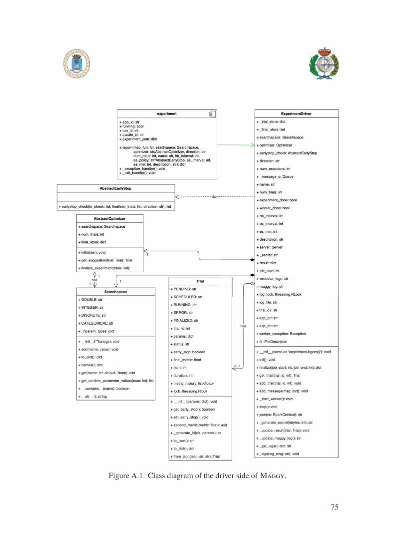
Figure A.1: Class diagram of the driver side of Maggy.

75

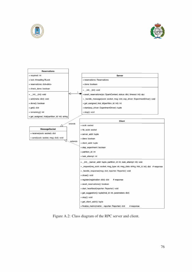
Figure A.2: Class diagram of the RPC server and client.

76

Figure A.3: Runtime of starting a Maggy experiment, showing how the different actors

get set up and interact before the actual communication protocol begins.

77

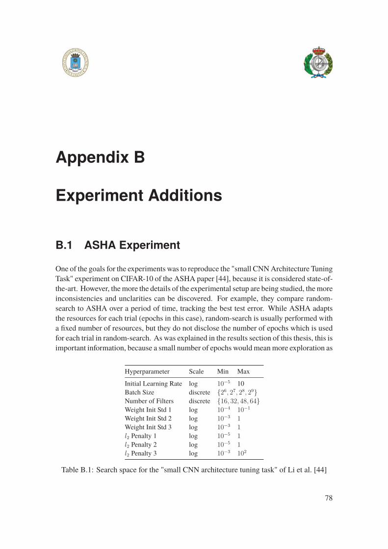
Appendix B

Experiment Additions

B.1 ASHA Experiment

One of the goals for the experiments was to reproduce the "small CNN Architecture Tuning

Task" experiment on CIFAR-10 of the ASHA paper [44], because it is considered state-of-

the-art. However, the more the details of the experimental setup are being studied, the more

inconsistencies and unclarities can be discovered. For example, they compare random-

search to ASHA over a period of time, tracking the best test error. While ASHA adapts

the resources for each trial (epochs in this case), random-search is usually performed with

a fixed number of resources, but they do not disclose the number of epochs which is used

for each trial in random-search. As was explained in the results section of this thesis, this is

important information, because a small number of epochs would mean more exploration as

Hyperparameter Scale Min Max

Initial Learning Rate log 10−5 10

Batch Size discrete {26, 27, 28, 29}Number of Filters discrete {16, 32, 48, 64}Weight Init Std 1 log 10−4 10−1

Weight Init Std 2 log 10−3 1

Weight Init Std 3 log 10−3 1

l2 Penalty 1 log 10−5 1

l2 Penalty 2 log 10−5 1

l2 Penalty 3 log 10−3 102

Table B.1: Search space for the "small CNN architecture tuning task" of Li et al. [44]

78

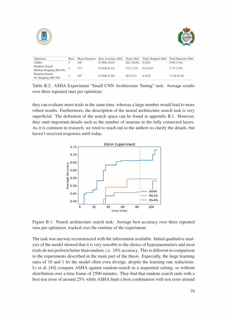
Optimizer Runs Mean Duration Best Accuracy (Std) Trials (Std) Trials Stopped (Std) Trial Duration (Std)

ASHA 3 105 0.7004 (0.03) 422 (38.69) 0 (0.0) 0.98 (3.54)

Random Search

Median Stopping (RS-ES)3 115 0.5438 (0.12) 112 (7.53) 63 (6.43) 5.75 (7.39)

Random Search

No Stopping (RS-NS)3 107 0.5306 (0.28) 40 (4.51) 0 (0.0) 17.20 (0.18)

Table B.2: ASHA Experiment "Small CNN Architecture Tuning" task: Average results

over three repeated runs per optimizer.

they can evaluate more trials in the same time, whereas a large number would lead to more

robust results. Furthermore, the description of the neural architecture search task is very

superficial. The definition of the search space can be found in appendix B.1. However,

they omit important details such as the number of neurons in the fully connected layers.

As it is common in research, we tried to reach out to the authors to clarify the details, but

haven’t received responses until today.

Figure B.1: Neural architecture search task: Average best accuracy over three repeated

runs per optimizer, tracked over the runtime of the experiment.

The task was anyway reconstructed with the information available. Initial qualitative anal-

ysis of the model showed that it is very sensible to the choice of hyperparameters and most

trials do not perform better than random, i.e. 10% accuracy. This is different in comparison

to the experiments described in the main part of the thesis. Especially, the large learning

rates of 10 and 1 let the model often even diverge, despite the learning rate reductions.

Li et al. [44] compare ASHA against random-search in a sequential setting, so without

distribution over a time frame of 2500 minutes. They find that random search ends with a

best test error of around 25% while ASHA finds a best combination with test error around

79

20% and overall being twice as fast in finding a combination with 25% test error. How-

ever, without knowing the number of epochs used for random-search this result is not very

strong. Since the models are so sensitive, a very low resource for random-search could

have led to similar results, because it can be that ASHA just evaluated many more tri-

als in the beginning. Therefore, we compared ASHA with distribution to random-search

with early stopping, to investigate if early stopping can eliminate the speedup of ASHA

compared to random search.

It can be observed, that in contrast to the previous experiments, for this search task, the

model complexity influenced the time needed for one epoch. Hence, each run of ASHA

manages to evaluate a different amount of trials, verifying the randomness of the approach.

ASHA is also able to evaluate a magnitude of trials more than synchronous SHA, as we

observed before. While ASHA reached the 75% accuracy in one run, on average the three

runs only return a 70% best accuracy, which gets close to the 25% test error reported by

Li et al. [44]. RS-ES can not compete on this example and returns only an 54% average

accuracy after the runtime of the experiment. However, again looking at the point up to

which the maximum resource used per trial is 64 epochs, ASHA also achieved only about

65% accuracy, still outperforming the other two optimizers. Since the model is sensitive

to the hyperparameter configuration, RS-ES is able to outperform random-search without

early stopping. This substantiates our observation, that early stopping is mainly beneficial

in this case.

To summarize, we could not reproduce the results of the paper with the information given.

In general, this example was added to show that instable models can lead to differing train-

ing times for the models, in contrast to the observations made in the small scale examples

of section 5.1. An additional reason to add this discussion, was to show that reproducabil-

ity for Auto-ML experiments is a great issue and should be tackled with future work.

80

Glossary

Auto-ML Auto-ML attempts to construct machine learning programs (specified by E , T

and P in the definition of machine learning), without human assistance and within

limited computational budgets [12]. 7, 8

convolutional neural network Inspired by the human visual system’s structure, convo-

lutional neural networks are a class of deep neural networks, mainly applied to com-

puter vision tasks [17]. 53

deep learning Deep Learning is a field of machine learning using artificial neural net-

works. Deep learning usually refers to the application of neural networks with many

hidden layers [3]. 1

hyperparameter In machine learning, a hyperparameter is a parameter whose value has

to be set statically and can’t be learned by the training process. 1

machine learning A computer program is said to learn from experienceE with respect to

some classes of task T and performance measure P if its performance can improve

with E on T measured by P [56]. 1

reinforcement learning Reinforcement learning models the problem of an agent that

needs to adapt its behaviour to a dynamic environment. The agent learns behav-

ior through trial-and-error interactions with the environment, getting a feedback at

each iteration to update its strategy [39]. 18

remote procedure call Remote procedure call is a protocol that allows a program to ex-

ecute a service of a program located on a computer in another address space over a

network without having to implement network communication details. 23

81

supervised machine learning Learns an unknown function from known input-output pairs

that maps inputs to outputs. 8

82

Acronyms

AI artificial intelligence. 1

API application programming interface. 4, 5, 22, 29, 32, 33, 38, 46, 48, 54, 64, 65, 73

ASHA Asynchronous Successive Halving Algorithm. 21, 31, 53–62, 64–67

CNN convolutional neural network. vii, viii, 53, 59, 78

DL deep learning. 1

FPGA Field-Programmable Gate Array. 2

GPU Graphics Processing Unit. 2, 3

HDFS Hadoop Distributed File System. 2

HPO hyperparameter optimization. 4, 7, 11–15, 34, 37, 57, 66

JVM Java Virtual Machine. 22

ML machine learning. 1, 8, 9, 13

NAS neural architecture search. 4, 7, 11, 16, 18, 59, 60, 65, 66

RPC remote procedure call. vii, 23, 37, 39, 41–43, 45–48, 52, 63, 64, 76

SGD Stochastic Gradient Descent. 55, 59

SHA Successive Halving Algorithm. viii, 56

83

TPU Tensor Processing Unit. 2

YARN Yet Another Resource Negotiator. 22

84