universidad politÉcnica de madridoa.upm.es/14785/1/lin_wang.pdf · energy flow contained in a...
TRANSCRIPT

UNIVERSIDAD POLITÉCNICA DE MADRID
ESCUELA TÉCNICA SUPERIOR DE INGENIEROS DE TELECOMUNICACIÓN
TESIS DOCTORAL
Advances in the Simultaneous Multiple Surface optical design method for imaging and non-imaging applications
Lin Wang Ingeniero en Electrónica
2012

UNIVERSIDAD POLITÉCNICA DE MADRID
Instituto de Energía Solar
Departamento de Electrónica Física
Escuela Técnica Superior de Ingenieros de Telecomunicación
TESIS DOCTORAL
Avances en método de diseño de Superficies Múltiples Simultáneas para aplicaciones en formación de imagen
y aplicaciones anidólicas
Advances in the Simultaneous Multiple Surface optical design method for imaging and non-imaging applications
AUTOR: D. Lin Wang Ingeniero en Electrónica
DIRECTOR: D. Pablo Benítez Giménez Doctor en Ingeniería de Telecomunicación
2012


Tribunal nombrado por el Magfco. Y Excmo. Sr. Rector de la Universidad Politécnica de Madrid. PRESIDENTE: VOCALES: SECRETARIO: SUPLENTES:
Realizado el acto de defensa y lectura de la Tesis en Madrid, el día ___ de _____ de 2012.
Calificación: EL PRESIDENTE LOS VOCALES EL SECRETARIO

Agradecimiento
Esta tesis empezó en octubre de 2007, después de que Pablo Benítez y Juan Carlos
Miñano me ofrecieran la posibilidad a hacer mi doctorado en Madrid. Jamás pensé
que un día llegara a ser capaz de hablar español, así como tampoco podía llegar a
imaginar la gran formación y enseñanzas que iba a recibir en este maravilloso grupo.
Durante esta tesis me han brindado numerosos consejos y guías vitales para mi
investigación, que me han servido para afrontar con éxito los constantes retos que me
han ido apareciendo, algo que solamente ha sido posible con la constante ayuda que
he recibido por parte de mis profesores y compañeros.
Por supuesto, mi primer agradecimiento va dirigido a Pablo Benítez y Juan Carlos
Miñano por esta preciosa oportunidad y su enorme apoyo en todo momento.
Quería agradecer a José Infante por compartir conmigo conocimientos de óptica, así
como el lugar de trabajo. Asimismo, quiero hacer llegar un agradecimiento al resto
del grupo de óptica: Dejan Grabovičkić, Pablo Zamora, Marina Buljan, Jiayao Liu,
Guillermo Biot, Jesús López y Hammed Ahmadpanahi y a todo el personal del Cedint
por hacer el ambiente de trabajo muy agradable. Quería agradecer a Julio Chaves el
enseñarme el uso de Mathematica con gran paciencia, a José Blen Flores por darme la
primera clase en C++, y también a otros investigadores de LPI con los que he
trabajado directamente en el desarrollo de la tesis, especialmente Fernando Muñoz,
Maikel Hernández, Rubén Mohedano, Aleksandra Cvetković y Juan Vilaplana.
Finalmente, a mi mujer Jing Cheng por acompañarme todos los días durante mi
estudio, al pequeño XiXi por darnos tantas alegrías, y también al resto de mi familia.
Tengo que agradecéroslo con todo mi amor.


Abstract
Classical imaging optics has been developed over centuries in many areas, such as its
paraxial imaging theory and practical design methods like multi-parametric
optimization techniques. Although these imaging optical design methods can provide
elegant solutions to many traditional optical problems, there are more and more
new design problems, like solar concentrator, illumination system, ultra-compact
camera, etc., that require maximum energy transfer efficiency, or ultra-compact
optical structure. These problems do not have simple solutions from classical
imaging design methods, because not only paraxial rays, but also non-paraxial rays
should be well considered in the design process.
Non-imaging optics is a newly developed optical discipline, which does not aim to
form images, but to maximize energy transfer efficiency. One important concept
developed from non-imaging optics is the “edge-ray principle”, which states that the
energy flow contained in a bundle of rays will be transferred to the target, if all its
edge rays are transferred to the target. Based on that concept, many CPC solar
concentrators have been developed with efficiency close to the thermodynamic limit.
When more than one bundle of edge-rays needs to be considered in the design, one
way to obtain solutions is to use SMS method. SMS stands for Simultaneous Multiple
Surface, which means several optical surfaces are constructed simultaneously.
The SMS method was developed as a design method in Non-imaging optics during
the 90s. The method can be considered as an extension to the Cartesian Oval
calculation. In the traditional Cartesian Oval calculation, one optical surface is built

to transform an input wave-front to an out-put wave-front. The SMS method
however, is dedicated to solve more than 1 wave-fronts transformation problem. In
the beginning, only 2 input wave-fronts and 2 output wave-fronts transformation
problem was considered in the SMS design process for rotational optical systems or
free-form optical systems. Usually “SMS 2D” method stands for the SMS procedure
developed for rotational optical system, and “SMS 3D” method for the procedure for
free-form optical system. Although the SMS method was originally employed in non-
imaging optical system designs, it has been found during this thesis that with the
improved capability to design more surfaces and control more input and output
wave-fronts, the SMS method can also be applied to imaging system designs and
possesses great advantage over traditional design methods.
In this thesis, one of the main goals to achieve is to further develop the existing SMS-
2D method to design with more surfaces and improve the stability of the SMS-2D
and SMS-3D algorithms, so that further optimization process can be combined with
SMS algorithms. The benefits of SMS plus optimization strategy over traditional
optimization strategy will be explained in details for both rotational and free-form
imaging optical system designs. Another main goal is to develop novel design
concepts and methods suitable for challenging non-imaging applications, e.g. solar
concentrator and solar tracker.
This thesis comprises 9 chapters and can be grouped into two parts: the first part
(chapter 2-5) contains research works in the imaging field, and the second part
(chapter 6-8) contains works in the non-imaging field. In the first chapter, an
introduction to basic imaging and non-imaging design concepts and theories is given.
Chapter 2 presents a basic SMS-2D imaging design procedure using meridian rays. In
this chapter, we will set the imaging design problem from the SMS point of view, and
try to solve the problem numerically. The stability of this SMS-2D design procedure
will also be discussed. The design concepts and procedures developed in this chapter
lay the path for further improvement.

Chapter 3 presents two improved SMS 3 surfaces’ design procedures using meridian
rays (SMS-3M) and skew rays (SMS-1M2S) respectively. The major improvement has
been made to the central segments selections, so that the whole SMS procedures
become more stable compared to procedures described in Chapter 2. Since these
two algorithms represent two types of phase space sampling, their image forming
capabilities are compared in a simple objective design.
Chapter 4 deals with an ultra-compact SWIR camera design with the SMS-3M
method. The difficulties in this wide band camera design is how to maintain high
image quality meanwhile reduce the overall system length. This interesting camera
design provides a playground for the classical design method and SMS design
methods. We will show designs and optical performance from both classical design
method and the SMS design method. Tolerance study is also given as the end of the
chapter.
Chapter 5 develops a two-stage SMS-3D based optimization strategy for a 2 freeform
mirrors imaging system. In the first optimization phase, the SMS-3D method is
integrated into the optimization process to construct the two mirrors in an accurate
way, drastically reducing the unknown parameters to only few system configuration
parameters. In the second optimization phase, previous optimized mirrors are
parameterized into Qbfs type polynomials and set up in code V. Code V optimization
results demonstrates the effectiveness of this design strategy in this 2-mirror system
design.
Chapter 6 shows an etendue-squeezing condenser optics, which were prepared for
the 2010 IODC illumination contest. This interesting design employs many non-
imaging techniques such as the SMS method, etendue-squeezing tessellation, and
groove surface design. This device has theoretical efficiency limit as high as 91.9%.
Chapter 7 presents a freeform mirror-type solar concentrator with uniform
irradiance on the solar cell. Traditional parabolic mirror concentrator has many
drawbacks like hot-pot irradiance on the center of the cell, insufficient use of active
cell area due to its rotational irradiance pattern and small acceptance angle. In order

to conquer these limitations, a novel irradiance homogenization concept is
developed, which lead to a free-form mirror design. Simulation results show that the
free-form mirror reflector has rectangular irradiance pattern, uniform irradiance
distribution and large acceptance angle, which confirm the viability of the design
concept.
Chapter 8 presents a novel beam-steering array optics design strategy. The goal of
the design is to track large angle parallel rays by only moving optical arrays laterally,
and convert it to small angle parallel output rays. The design concept is developed as
an extended SMS method. Potential applications of this beam-steering device are:
skylights to provide steerable natural illumination, building integrated CPV systems,
and steerable LED illumination. Conclusion and future lines of work are given in
Chapter 9.

Resumen
La óptica de formación de imagen clásica se ha ido desarrollando durante siglos,
dando lugar tanto a la teoría de óptica paraxial y los métodos de diseño prácticos
como a técnicas de optimización multiparamétricas. Aunque estos métodos de
diseño óptico para formación de imagen puede aportar soluciones elegantes a
muchos problemas convencionales, siguen apareciendo nuevos problemas de diseño
óptico, concentradores solares, sistemas de iluminación, cámaras ultracompactas,
etc. que requieren máxima transferencia de energía o dimensiones ultracompactas.
Este tipo de problemas no se pueden resolver fácilmente con métodos clásicos de
diseño porque durante el proceso de diseño no solamente se deben considerar los
rayos paraxiales sino también los rayos no paraxiales.
La óptica anidólica o no formadora de imagen es una disciplina que ha evolucionado
en gran medida recientemente. Su objetivo no es formar imagen, es maximazar la
eficiencia de transferencia de energía. Un concepto importante de la óptica anidólica
son los “rayos marginales”, que se pueden utilizar para el diseño de sistemas ya que
si todos los rayos marginales llegan a nuestra área del receptor, todos los rayos
interiores también llegarán al receptor. Haciendo uso de este principio, se han
diseñado muchos concentradores solares que funcionan cerca del límite teórico que
marca la termodinámica. Cuando consideramos más de un haz de rayos marginales
en nuestro diseño, una posible solución es usar el método SMS (Simultaneous
Multiple Surface), el cuál diseña simultáneamente varias superficies ópticas.

El SMS nació como un método de diseño para óptica anidólica durante los años 90.
El método puede ser considerado como una extensión del cálculo del óvalo
cartesiano. En el método del óvalo cartesiano convencional, se calcula una superficie
para transformar un frente de onda entrante a otro frente de onda saliente. El
método SMS permite transformar varios frentes de onda de entrada en frentes de
onda de salida. Inicialmente, sólo era posible transformar dos frentes de onda con
dos superficies con simetría de rotación y sin simetría de rotación, pero esta
limitación ha sido superada recientemente. Nos referimos a “SMS 2D” como el
método orientado a construir superficies con simetría de rotación y llamamos “SMS
3D” al método para construir superficies sin simetría de rotación o free-form.
Aunque el método originalmente fue aplicado en el diseño de sistemas anidólicos, se
ha observado que gracias a su capacidad para diseñar más superficies y controlar
más frentes de onda de entrada y de salida, el SMS también es posible aplicarlo a
sistemas de formación de imagen proporcionando una gran ventaja sobre los
métodos de diseño tradicionales.
Uno de los principales objetivos de la presente tesis es extender el método SMS-2D
para permitir el diseño de sistemas con mayor número de superficies y mejorar la
estabilidad de los algoritmos del SMS-2D y SMS-3D, haciendo posible combinar la
optimización con los algoritmos. Los beneficios de combinar SMS y optimización
comparado con el proceso de optimización tradicional se explican en detalle para
sistemas con simetría de rotación y sin simetría de rotación. Otro objetivo
importante de la tesis es el desarrollo de nuevos conceptos de diseño y nuevos
métodos en el área de la concentración solar fotovoltaica.
La tesis está estructurada en 9 capítulos que están agrupados en dos partes: la
primera de ellas (capítulos 2-5) se centra en la óptica formadora de imagen mientras
que en la segunda parte (capítulos 6-8) se presenta el trabajo del área de la óptica
anidólica. El primer capítulo consta de una breve introducción de los conceptos
básicos de la óptica anidólica y la óptica en formación de imagen.
El capítulo 2 describe un proceso de diseño SMS-2D sencillo basado en los rayos
meridianos. En este capítulo se presenta el problema de diseñar un sistema

formador de imagen desde el punto de vista del SMS y se intenta obtener una
solución de manera numérica. La estabilidad de este proceso se analiza con detalle.
Los conceptos de diseño y los algoritmos desarrollados en este capítulo sientan la
base sobre la cual se realizarán mejoras.
El capítulo 3 presenta dos procedimientos para el diseño de un sistema con 3
superficies SMS, el primero basado en rayos meridianos (SMS-3M) y el segundo
basado en rayos oblicuos (SMS-1M2S). La mejora más destacable recae en la
selección de los segmentos centrales, que hacen más estable todo el proceso de
diseño comparado con el presentado en el capítulo 2. Estos dos algoritmos
representan dos tipos de muestreo del espacio de fases, su capacidad para formar
imagen se compara diseñando un objetivo simple con cada uno de ellos.
En el capítulo 4 se presenta un diseño ultra-compacto de una cámara SWIR diseñada
usando el método SMS-3M. La dificultad del diseño de esta cámara de espectro
ancho radica en mantener una alta calidad de imagen y al mismo tiempo reducir
drásticamente sus dimensiones. Esta cámara es muy interesante para comparar el
método de diseño clásico y el método de SMS. En este capítulo se presentan ambos
diseños y se analizan sus características ópticas.
En el capítulo 5 se describe la estrategia de optimización basada en el método SMS-
3D. El método SMS-3D calcula las superficies ópticas de manera precisa, dejando
sólo unos pocos parámetros libres para decidir la configuración del sistema.
Modificando el valor de estos parámetros se genera cada vez mediante SMS-3D un
sistema completo diferente. La optimización se lleva a cabo variando los
mencionados parámetros y analizando el sistema generado. Los resultados muestran
que esta estrategia de diseño es muy eficaz y eficiente para un sistema formado por
dos espejos.
En el capítulo 6 se describe un sistema de compresión de la Etendue, que fue
presentado en el concurso de iluminación del IODC en 2010. Este interesante diseño
hace uso de técnicas propias de la óptica anidólica, como el método SMS, el teselado
de las lentes y el diseño mediante grooves. Este dispositivo tiene un límite teórica en
la eficiencia del 91.9%.

El capítulo 7 presenta un concentrador solar basado en un espejo free-form con
irradiancia uniforme sobre la célula. Los concentradores parabólicos tienen
numerosas desventajas como los puntos calientes en la zona central de la célula, uso
no eficiente del área de la célula al ser ésta cuadrada y además tienen ángulos de
aceptancia de reducido. Para poder superar estas limitaciones se propone un
novedoso concepto de homogeneización de la irrandancia que se materializa en un
diseño con espejo free-form. El análisis mediante simulación demuestra que la
irradiancia es homogénea en una región rectangular y con mayor ángulo de
aceptancia, lo que confirma la viabilidad del concepto de diseño.
En el capítulo 8 se presenta un novedoso concepto para el diseño de sistemas
afocales dinámicos. El objetivo del diseño es realizar un sistema cuyo haz de rayos de
entrada pueda llegar con ángulos entre ±45º mientras que el haz de rayos a la salida
sea siempre perpendicular al sistema, variando únicamente la posición de los
elementos ópticos lateralmente. Las aplicaciones potenciales de este dispositivo son
varias: tragaluces que proporcionan iluminación natural, sistemas de concentración
fotovoltaica integrados en los edificios o iluminación direccionable con LEDs.
Finalmente, el último capítulo contiene las conclusiones y las líneas de investigación
futura.

Contents
1
Contents
Chapter 1. Introduction ............................................................................................................................. 3
1.1. Basic concepts in Geometric Optics ........................................................................................... 3 1.1.1. Hamiltonian system .......................................................................................................... 3 1.1.2. Phase space ........................................................................................................................ 4 1.1.3. Étendue .............................................................................................................................. 5 1.1.4. Eikonal function ................................................................................................................ 6 1.2. Generalized Cartesian Oval and the SMS method ..................................................................... 6 1.2.1. The SMS chain .................................................................................................................. 8 1.2.2. Integrability condition ....................................................................................................... 8 1.3. Design problems of imaging and non-imaging optics ................................................................ 9 1.3.1. Aberration theory of imaging optics ................................................................................ 10 1.3.2. The modulation transfer function MTF ........................................................................... 12 1.3.3. Edge ray principle of non-imaging optics ........................................................................ 12
Chapter 2. SMS imaging design of rotational optics using meridian rays .............................................. 15 2.1. Introduction ......................................................................................................................... 15
2.1.1. Aplanatic imaging design problem ................................................................................. 16 2.1.2. SMS imaging design problem ........................................................................................ 18
2.2. SMS Design procedures ...................................................................................................... 20 2.2.1. Central conditions for SMS 3 and 4 surfaces .................................................................. 21 2.2.2. Recursive SMS construction ........................................................................................... 24
2.3. Results and Analysis ........................................................................................................... 28 2.3.1. Instability analysis of SMS 3-surface designs ................................................................ 28 2.3.2. SMS designs vs. Aplanatic designs ................................................................................ 32
2.4. Conclusions ......................................................................................................................... 35
Chapter 3. Improved SMS algorithms and parametric optimization ...................................................... 37 3.1. Introduction ......................................................................................................................... 37 3.2. Phase space sampling .......................................................................................................... 38 3.3. Improved SMS algorithms .................................................................................................. 41 3.3.1. Wave-front propagation ................................................................................................... 42 3.3.2. Improved SMS-3M algorithms ........................................................................................ 44 3.3.3. SMS-1M2S algorithm ..................................................................................................... 46 3.4. A simple objective design example ..................................................................................... 48 3.5. Conclusion ........................................................................................................................... 52
Chapter 4. Ultra-compact SWIR telephoto camera design ..................................................................... 54 4.1. Design background .............................................................................................................. 54 4.2. Specifications of the telephoto camera ................................................................................ 56 4.3. Two candidate optical structures ......................................................................................... 57 4.3.1. RXXR type optical structures .......................................................................................... 58 4.3.2. XRXR type optical structures .......................................................................................... 65 4.4. Conclusion ........................................................................................................................... 67
Chapter 5. SMS imaging design in three dimensions ............................................................................. 70 5.1. Introduction ......................................................................................................................... 70 5.2. Problem description ............................................................................................................. 71 5.3. SMS3D design procedures .................................................................................................. 75

Lin Wang
2
5.4. Phase I: Free parameters optimization ................................................................................. 77 5.4.1. “4” type configurations ................................................................................................... 77 5.4.2. “N” type configurations .................................................................................................. 80 5.5. Phase II: Free form surfaces optimization ........................................................................... 83 5.6. Conclusion and future work ................................................................................................ 85
Chapter 6. Étendue-squeezing condenser optics..................................................................................... 87 6.1. Statement of the problem..................................................................................................... 87 6.2. Collimator design with grooved mirrors ............................................................................ 88 6.2.1. Collimator design with SMS-2D method ....................................................................... 90 6.2.2. Grooved lens.................................................................................................................... 92 6.3. Étendue-squeezing lens array .............................................................................................. 95 6.3.1. Étendue squeezer design .................................................................................................. 96 6.3.2. Étendue-squeezer tessellation .......................................................................................... 97 6.4. Complete system analysis.................................................................................................. 100 6.5. Conclusion ......................................................................................................................... 103
Chapter 7. Single Free-Form reflector design for concentration photovoltaic ..................................... 104 7.1. Introduction ....................................................................................................................... 104 7.2. Analytical model for parabolic concentrator ..................................................................... 106 7.2.1. Calculations with small solar cell approximation .......................................................... 106 7.2.2. Formation of hot spot .................................................................................................... 109 7.3. Min-max variation problem for uniform irradiance on solar cell ...................................... 110 7.3.1. Close fit parabolic mirror approximation ...................................................................... 110 7.3.2. Formulation of min-max variational problem ............................................................... 111 7.3.3. Integrability condition for displacement function ......................................................... 113 7.3.4. Tangential condition ...................................................................................................... 114 7.3.5. Numerical solution ........................................................................................................ 115 7.4. Design Examples ............................................................................................................... 119 7.5. Conclusion ......................................................................................................................... 122
Chapter 8 . Time-varying SMS optics ................................................................................................. 124 8.1. Introduction ....................................................................................................................... 124 8.2. Straight-path moving optics in two dimensions ................................................................ 126 8.2.1. Design principles ........................................................................................................... 126 8.2.2. Design example ............................................................................................................. 129 8.3. Curve-path moving optics in two dimensions ................................................................... 130 8.3.1. Calculation of the trajectory .......................................................................................... 130 8.3.2. SMS construction of lens profiles ................................................................................. 133 8.3.3. 2D design example ........................................................................................................ 134 8.3.4. 3Dotational design example .......................................................................................... 136 8.4. Conclusions ....................................................................................................................... 139
Conclusions and future lines of investigations ..................................................................................... 141 Appendix A. Surface construction using Cubic Local Patches (CLP) ................................................. 145 Appendix B. SMS3D skinning with scaled initial patch ...................................................................... 150 Publications .......................................................................................................................................... 154

Chapter 1 Introduction
3
Chapter 1. Introduction
1.1. Basic concepts in Geometric Optics
Geometric optics is an approximation to wave optics, when the light’s
wavelength is considered as infinitesimal small. That condition is usually satisfied in
the scale of most real-life applications, where size of optical systems is much bigger
than the light’s wavelength. Due to this fact, in a traditional optical system design like
a digital camera, the effect of lights’ diffraction is usually studied after geometric
design procedures. However, realizing that nowadays optical systems are becoming
smaller and requiring higher quality, the analysis of diffraction effects will play a
more important role.
1.1.1. Hamiltonian system [1,2]
A comprehensive model developed in geometric optics is the Hamiltonian system,
from where came many fundamental concepts. It's very common to deduce the
Hamiltonian system from Fermat’s principle of stationary optical path as a solution to
a variation problem expressed in Cartesian coordinates:
1
0
2 20 ( , , ) 1z
c c zL L n x y z x y dzδ = = + +∫ (1.1)
Where Lc is the optical path length of the light ray that passes through a space with
material index distribution n(x,y,z). In this variation problem, the unknowns are the
light trajectory that can give minimum optical path length, or functions x(z) and y(z).
With this choice of parameters, the Euler’s equations of light path are expressed as:

Lin Wang
4
2 2
2 2
2 2
2 2
[ ] 1 01
[ ] 1 01
x
y
d nx n x ydz x yd ny n x ydz x y
− + + = + + − + + = + +
(1.2)
Which is a second order differential equation system. If we define the following
quantities (p, q, r) as optical direction cosines:
2 2
2 2
2 2
1
1
1
nxpx ynyqx ynrx y
=
+ + =
+ + = + +
(1.3)
With condition that 2 2 2 2p q r n+ + = , we can transform the above second differential
equation system into a system a first order differential equation system, which is a
special form of Hamilton system:
2 2 2
,
,p x
q y
x H p Hy H q H
H n p q
= = − = = −
= − −
(1.4)
Similar deduction can be applied if the independent variable is not the z coordinate
but the time t, and Hamiltonian system obtains its highly symmetrical form as:
2 2 2 2
,
,
,
0
p x
q y
q y
x H p Hy H q Hz H r H
H n p q r
= = − = = − = = − = − − − ≡
(1.5)
In this last representation, optical direction cosines (p, q, r) are as equal important as
position variables (x, y, z), which leads to the effort to discuss solutions in a more
comprehensive space, the phase space.
1.1.2. Phase space[3,4]
In phase space, each point depicts both the position of a light ray and its
propagation direction at that point; ray-bundles are then represented as a volume of
positions. Ray propagation in three dimension (x,y,z) with material index distribution
n(x,y,z) defines a trajectory in the phase space; propagation of one initial ray-bundle
Chapter 1 Introduction
5
through a certain material is similarly defined as the transformation from one volume
of initial positions into another volume of final positions as a function of time. For
example, If all rays intersect a given surface at z=f(x,y), these rays together can be
fully described as a 4-dimentional bundle M4D(x,y,p,q) with the condition that
2 2 2r n p q= − − .
One special case often occurs in optical design when p and q are functions of x
and y, or p(x,y) and q(x,y). Then this bundle M4D(x,y,p(x,y),q(x,y)) of considered ray-
bundle degenerates to a two dimensional bundle M2D(x,y), which states that at each
intersection point (x,y) passes only one ray with a given direction.
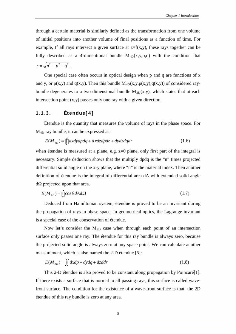
1.1.3. Étendue[4]
Étendue is the quantity that measures the volume of rays in the phase space. For
M4D ray bundle, it can be expressed as:
4( )DE M dxdydpdq dxdzdpdr dydzdqdr= + +∫ (1.6)
when étendue is measured at a plane, e.g. z=0 plane, only first part of the integral is
necessary. Simple deduction shows that the multiply dpdq is the “n” times projected
differential solid angle on the x-y plane, where “n” is the material index. Then another
definition of étendue is the integral of differential area dA with extended solid angle
dΩ projected upon that area.
4( ) cosDE M dAdθ= Ω∫ (1.7)
Deduced from Hamiltonian system, étendue is proved to be an invariant during
the propagation of rays in phase space. In geometrical optics, the Lagrange invariant
is a special case of the conservation of étendue.
Now let’s consider the M2D case when through each point of an intersection
surface only passes one ray. The étendue for this ray bundle is always zero, because
the projected solid angle is always zero at any space point. We can calculate another
measurement, which is also named the 2-D étendue [5]:
2( )DE M dxdp dydq dzddr= + +∫∫ (1.8)
This 2-D étendue is also proved to be constant along propagation by Poincaré[1].
If there exists a surface that is normal to all passing rays, this surface is called wave-
front surface. The condition for the existence of a wave-front surface is that: the 2D
étendue of this ray bundle is zero at any area.

Lin Wang
6
0dxdp dydq dzddr+ + = (1.9)
1.1.4. Eikonal function
In the presence of wave-front through a given 2D bundle of rays, we can define a
eikonal function “S” which satisfies the eikonal equation[4]: 2 2 2
2( ) ( , , )S S S n x y zx y z
∂ ∂ ∂+ + =
∂ ∂ ∂ (1.10)
and optical direction cosines are related to the eikonal function by:
, ,S S Sp q rx y z
∂ ∂ ∂= = =
∂ ∂ ∂ (1.11)
Or by a total differential:
dS pdx qdy rdz= + + (1.12)
Then it’s easy to calculate the eikonal function of 2D bundle of rays by integration of
Equation (1.12):
B
AS pdx qdy rdz= + +∫
(1.13)
Which is carried out along an ray path between point A
and B
. As has been seen in
Section 1.1.3 that the 2-D étendue for this type of 2D ray-bundle is preserved to be
zero along propagation, the eikonal function can then be acquired by integration along
an arbitrary path that connects point A
and B
.
1.2. Generalized Cartesian Oval and the SMS method
Generalized Cartesian Ovals are reflective or refractive surfaces that couple the
rays of one given input wave-front B1 onto another output wave-front B2, as shown in
Fig 1.1.
Fig 1.1 Generalized Cartesian Oval coupling one pair of wave-fronts

Chapter 1 Introduction
7
Suppose eikonal functions of wave-front B1 and Wave-front B2 are S1(x,y,z) and
S2(x,y,z) respectively, then the mirror surface should fulfill the condition that the two
eikonal functions are continuous on that mirror surface, which is a generalized
Cartesian oval:
1 2( , , ) ( , , )L x y z L x y z= (1.14)
This condition is also equivalent to the constant optical path length between input
and ouput wave-fronts through reflection or refracction. The generalized Cartesian
Oval has been applied already in imaging optics to construct an aspherical surface for
correction of axial spherical aberrations. Also in non-imaging optics, it’s the basis for
the “string method” from which many high efficiency CPC concentrators have been
developed [3,4].
There has aroused another question: since one surface can be constructed to
couple one pair of input and output wave-fronts, how about two pairs or even more
pairs of wave-fronts? The SMS method has been specifically developed to answer that
question by Miñano and Benitez and co-workers ever since the late 90s [6-9]. The
SMS theory states that one free-form surface is capable to couple one pair of wave-
fronts, while two free-form surfaces are capable to couple two pairs of wave-fronts, as
shown in Fig 1.2. In Blen’s thesis [9], SMS design procedures had been developed for
two free-form surfaces, which include three steps:
(1) The construction of seed rib;
(2) The construction of spine curves;
(3) The skinning through spine curve.
Fig 1.2 The SMS method coupling two pairs of wave-fronts.

Lin Wang
8
1.2.1. The SMS chain
Fig 1.3 explains how a SMS chain is obtained to couple two pair of wave-fronts:
(1) P0 is a predetermined point with its normal vector N0;
(2) Ray 1 comes from wave-front Wi2 and will be deflected after point P0 and P1
to Ray 2 of wave-front Wo2; P1 and its normal vector N1 are then calculated
by constant optical path length L2 between Wi2 and Wo2;
(3) Point P2 and its normal vector N2 are calculated to transmit Ray 3 from wave-
front Wo1 to wave-front Wi1 with constant optical path length condition L2;
(4) Repeat the above process to obtain the SMS chain.
The optical path lengths between two pairs of wave-fronts should be carefully
selected to make the chain integrable. Otherwise, interpolated curves through
calculated chain will not possess required normal vectors. Later, the SMS surfaces are
constructed through series of SMS chains.
Fig 1.3 SMS chain calculation
1.2.2. Integrability condition
When a point cloud with given normal vectors has to be interpolated by a smooth
surface, it has to fulfill the integrability condition to guarantee the existence of such a
surface:
( ) 0N N∇× = (1.14)
Ray 1
Ray 2
Ray 3
Ray 4

Chapter 1 Introduction
9
There exists a similarity between the existence of wave-front through a 2D ray-
bundle and the existence of interpolation surface through a point cloud. In the latter
case, normal vector N
can be considered as ray optical direction cosines (p, q, r) at
each location.
( , , )
( , , )
N p q r
r x y z
=
=
(1.15)
Therefore, the 2D étendue defined in previous section has also to be zero at the
interpolation surface S(u,v), where u and v are surface’s parameters. From Equations
(1.9) and (1.15), another equivalent condition is obtained:
. . 0u v v uN r N r− =
(1.16)
It’s often convenient in numerical calculation to expand condition (1.14) or (1.16)
into their difference equations under certain precision.
In the case of the Generalized Cartesian oval or SMS methods, the surface
integrability is ensured by design, but other design methods need to impose it
specifically.
1.3. Design problems of imaging and non-imaging optics
Classical geometrical optics has been developed over centuries from paraxial
optics to high order aberration theory, and most recently multiple-parametric
optimization with aid of high speed computer; however, non-imaging optics was only
founded in 1960s for solar concentrators. Their difference can be well illustrated in
Fig 1.4: for a imaging system, its primary goal is to establish a given mapping
between the object and image space; while for a non-imaging optics, the main
objective is to achieve as high as possible transmission efficiency light rays from a
light source to a certain receiver.
Lin Wang
10
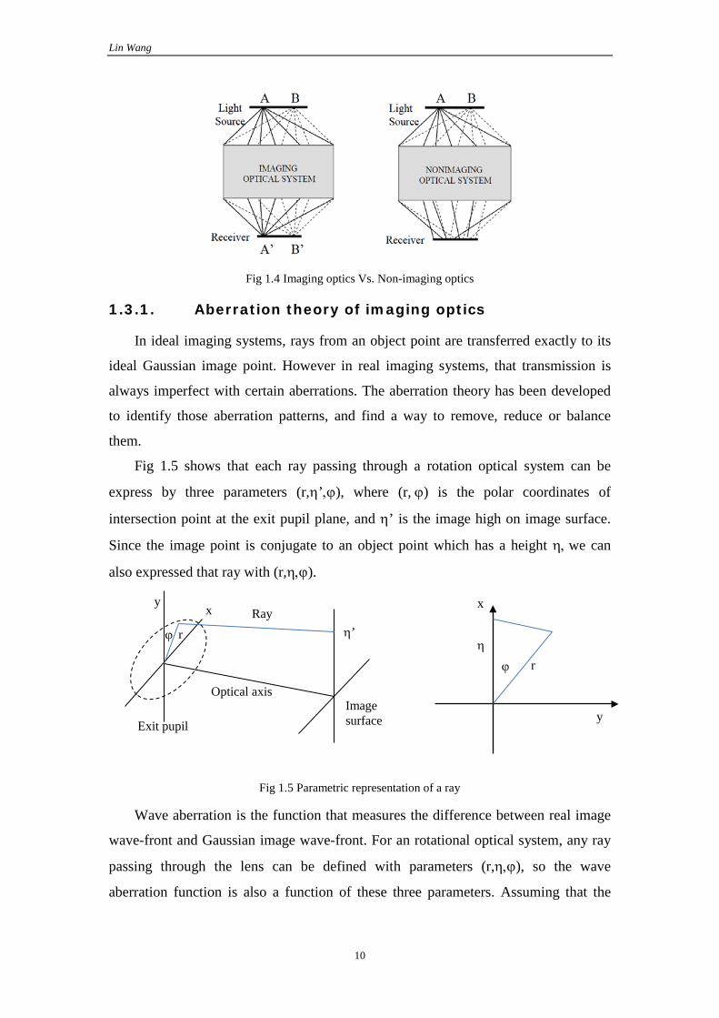
Fig 1.4 Imaging optics Vs. Non-imaging optics
1.3.1. Aberration theory of imaging optics
In ideal imaging systems, rays from an object point are transferred exactly to its
ideal Gaussian image point. However in real imaging systems, that transmission is
always imperfect with certain aberrations. The aberration theory has been developed
to identify those aberration patterns, and find a way to remove, reduce or balance
them.
Fig 1.5 shows that each ray passing through a rotation optical system can be
express by three parameters (r,η’,ϕ), where (r, ϕ) is the polar coordinates of
intersection point at the exit pupil plane, and η’ is the image high on image surface.
Since the image point is conjugate to an object point which has a height η, we can
also expressed that ray with (r,η,ϕ).
Fig 1.5 Parametric representation of a ray
Wave aberration is the function that measures the difference between real image
wave-front and Gaussian image wave-front. For an rotational optical system, any ray
passing through the lens can be defined with parameters (r,η,ϕ), so the wave
aberration function is also a function of these three parameters. Assuming that the
x
y Exit pupil
Optical axis
Ray r ϕ η’
Image surface
x y
r η
ϕ

Chapter 1 Introduction
11
wave aberration can be expressed as a power series into parameters (r, η, ϕ), we can
deduce [10]: 2
0 20
1 112
2 00
40 40
31 31
2 2 22 22
2 22 20
33 11
44 00
0
cos
cos
cos
cos
W W r DefocusW r Lateral image shiftW
W r Spherical aberrationW r ComaW r Astigmatism Third order aberrationW r Field curvatureW r Distortion
W
η φ
η
η φ
η φ
η
η φ
η
=+
+
+
+ + + +
+
+ 660
.W r Spherical aberration
Higher order aberrationetc
+
(1.17)
The existence of wave aberration leads to deviations between real rays’
intersection points at image plane and ideal image position, which is also called
transverse aberration as shown in Fig 1.6. The relationship between wave aberrations
and transverse aberrations has been established analytically in Ref [1].
Fig 1.6. Wave aberration and transverse ray aberrations
In Equation (1.17), the x-component and y-component of transverse ray
aberration are proportional to the partial derivatives of wave aberration and the radius
of reference sphere Rrs.

Lin Wang
12
''
''
rs
rs
R Wdn yR Wdn x
η
ζ
∂ = − ∂
∂ = − ∂
(1.17)
Although reference sphere can be placed at arbitrary position, it’s convenient to
do the calculation at the exit pupil position with relative pupil coordinates [1].
1.3.2. The modulation transfer function MTF
The optical transfer function (OTF) of an imaging system measures the optical
resolution (image sharpness) that the system is capable of without considering the
sensor’s resolution. The optical transfer function is defined in Equ. (1.18):
Im age ContrastOTFObject Contrast
= (1.18)
Where contrast is calculated from maximum and minimum object and image
intensities as:
max min
max min
I IContrastI I
−=
+ (1.19)
Under Fourier transformation, the OTF is represented as a vector quantity that
takes into account amplitude and phase variations, as shown in Equ. (1.20):
( )( ) ( ) iPTFOTF MTF e ωω ω= (1.20)
In practice, MTF which is the amplitude part of OTF function is what lens
designers are most concerned about, although the phase transfer function (PTF) can
have a secondary effect. If the PTF exceeds 180 degrees, which usually happens at
high special frequency, then it’s possible for MTF to become effectively negative,
which means a reverse of image contrast.
1.3.3. Edge ray principle of non-imaging optics
Since for a non-imaging system, its main objective is not imaging but to achieve
high transmission efficiency, this relaxation of imaging restrictions leads to a
fundamental design principle: the edge-ray principle. If we view the in the phase
space, rays from the light source form an input ray-bundle Mi and rays to the receiver
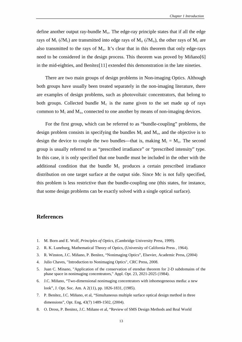
Chapter 1 Introduction
13
define another output ray-bundle Mo. The edge-ray principle states that if all the edge
rays of Mi (∂Mi) are transmitted into edge rays of Mo (∂Mo), the other rays of Mi are
also transmitted to the rays of Mo. It’s clear that in this theorem that only edge-rays
need to be considered in the design process. This theorem was proved by Miñano[6]
in the mid-eighties, and Benítez[11] extended this demonstration in the late nineties.
There are two main groups of design problems in Non-imaging Optics. Although
both groups have usually been treated separately in the non-imaging literature, there
are examples of design problems, such as photovoltaic concentrators, that belong to
both groups. Collected bundle Mc is the name given to the set made up of rays
common to Mi and Mo, connected to one another by means of non-imaging devices.
For the first group, which can be referred to as “bundle-coupling” problems, the
design problem consists in specifying the bundles Mi and Mo, and the objective is to
design the device to couple the two bundles—that is, making Mi = Mo. The second
group is usually referred to as “prescribed irradiance” or “prescribed intensity” type.
In this case, it is only specified that one bundle must be included in the other with the
additional condition that the bundle Mc produces a certain prescribed irradiance
distribution on one target surface at the output side. Since Mc is not fully specified,
this problem is less restrictive than the bundle-coupling one (this states, for instance,
that some design problems can be exactly solved with a single optical surface).
References 1. M. Born and E. Wolf, Principles of Optics, (Cambridge University Press, 1999).
2. R. K. Luneburg, Mathematical Theory of Optics, (University of California Press , 1964).
3. R. Winston, J.C. Miñano, P. Benítez, “Nonimaging Optics”, Elsevier, Academic Press, (2004)
4. Julio Chaves, "Introduction to Nonimaging Optics", CRC Press, 2008.
5. Juan C. Minano, "Application of the conservation of etendue theorem for 2-D subdomains of the phase space in nonimaging concentrators," Appl. Opt. 23, 2021-2025 (1984).
6. J.C. Miñano, “Two-dimensional nonimaging concentrators with inhomogeneous media: a new
look”, J. Opt. Soc. Am. A 2(11), pp. 1826-1831, (1985).
7. P. Benítez, J.C. Miñano, et al, “Simultaneous multiple surface optical design method in three
dimensions”, Opt. Eng, 43(7) 1489-1502, (2004).
8. O. Dross, P. Benitez, J.C. Miñano et al, “Review of SMS Design Methods and Real World

Lin Wang
14
Applications”, SPIE, San Diego (2004).
9. José Blen Flores, Doctoral Thesis “Design of multiple free-form optical surfaces in 3D” E.T.S.I.Telecomunicación, (2007).
10. Michael J. Kidger, Fundamental optical design, (SPIE Press, 2001).
11. P. Benitez, “Conceptos avanzados de óptica anidólica: diseño y fabricación”, Thesis Doctoral,
E.T.S.I.Telecomunicación, Madrid (1998).
Chapter 2 SMS imaging design of rotational optics using meridian rays
15
Chapter 2. SMS imaging design of rotational optics using meridian rays
2.1. Introduction
A typical imaging design problem is to find an optical system with several
spherical or aspherical surfaces, through which rays propagate from object space to
image space and form images. An ideal imaging system can produce stigmatic images
for all object points. Planar mirror is the only known device that is capable of perfect
imaging with unit magnification. Another theoretical model is Maxwell’s fish eye,
which uses a gradient index material [1]. However, perfect imaging between object
space and image space is usually not required, because a perfect imaging instrument
has been proven to be a trivial case in the optical design. The magnification of a
perfect instrument is determined only by the refractive indices of object space and
image space [1]. Therefore, the common task of most optical designs is not to find a
perfect imaging system, but to find a balance between performance and
manufacturability.
Classical Imaging design [2, 3, 4] is based on maximizing a merit function that
measures image quality over a prescribed field of view. This maximization is obtained
by parametrically varying the optical surfaces. When spherical sections were the only
surface shape used, the merit function was based on analytical aberration calculations
[5]. Later on, multi-parametric optimization techniques were used to maximize much
more complex merit functions [6]. Today, multi-parametric optimization is a common
tool of any optical design software. The algorithms progress from an initial guess to

Lin Wang
16
the final solution. Since the search is local there is no guarantee that the algorithm will
find the absolute maximum.
The use of aspheric surfaces has not changed the basic optimization methodology.
An aspheric surface is conventionally described by the following function [3]:
2
4 6 84 6 82 21 1 (1 )
cz a a a
c k
ρρ ρ ρ
ρ= + + + +
+ − + (2.1)
where ρ is the distance from a point to the optical axis (z axis), c is the vertex radius
of curvature. The remaining parameters (k, a4, a6, …) describe the “asphericity” of
the surface. More effective ways to describe aspheric surfaces are based on
orthogonal polynomials as Zernike’s and recently proposed by Forbes [7].
The optimization strategy with aspherics usually starts with a spherical design. The
final aspheric surface is not “far” from this initial spherical design, mainly because
there are many local maxima where the optimization process finds a solution.
Sometime the optimization process adds new parameters to optimize as the process
progresses: first starting with k (with the initial value k=0 for the spherical surface)
until a local maximum is found and then following with a4, etc. In practice, the
performance of the design does not improve when the number of optimizing
parameters is big (>10) because the asphericity of one surface is just cancelling the
asphericity of another [4].
2.1.1. Aplanatic imaging design problem
Aplanatic two-surface designs are long known through the work of Schwarzschild
[9], Wassermann and Wolf [10], Welford [11], Mertz [12, 13] and others. Recently
Lynden-Bell and Willstrop derived an analytic expression of general two-mirror
aplanats, [14, 15].
Aplanatic systems are axisymmetric optical designs free from spherical aberration
and linear coma at the axial direction of all orders. These two conditions entail these
other two design conditions: (1) stigmatic image of the axial direction (note that all
the rays involved in this condition are exclusively tangential) and (2) the Abbe sine
condition. The contrary statement is also true: a design forming stigmatic on-axis
image and fulfilling the Abbe sine condition is aplanatic. Abbe sine condition can be
derived from the condition of zero linear coma, but this is only one point of view. For

Chapter 2 SMS imaging design of rotational optics using meridian rays
17
instance, Clausius, who derived the Abbe condition in 1864, did it from
thermodynamic arguments [11] (we can also say that he used the conservation of
etendue theorem [16]). In 1884, Hockin gave a proof using path differences along
tangential rays (without considering sagittal rays) [11]. Because the Abbe sine
condition can be derived by imposing the zero coma condition only on tangential rays,
we can say that the aplanatic are a set of 2D design conditions since they can be
imposed and checked using only tangential rays. Additionally, aplanatic systems
result to be free of linear coma also for the sagittal rays near the axis, but this fact
does not need to be used in the design procedure, it is just a fortunate consequence of
the symmetry regardless that the design procedure is purely 2D (surprisingly a
requirement imposed solely on cones of light corresponding to the on-axis points
affects the quality of imaging nearby off-axis points [17]).
Fig 2.1. Numerical aplanatic design algorithm: a thick lens design
Two aplanatic conditions enable us to calculate two optical surfaces

Lin Wang
18
simultaneously. An aplanatic design can be realized by numerical approximation
algorithm. Fig 2.1 shows a recursive algorithm with tangential approximation applied
to a simple aplanatic lens design:
a) To start the process, an object point A, two vertices of the lens (B,C) and an image
point D are selected along the optical axis; Optical path length “L” between point
A and D is defined by: L Constant = d10 + nd20 + d30
b) Any pair of lens’ points along a ray should define a ray-path with constant optical
path length: d1 + nd2 + d3 = L Constant; Also, abbe sine condition require that object
angle q1 and image angle q2 should satisfy: sin(θ1) = M sin(θ2), where M is a
constant angular magnification.
c) Starting from center, we select one ray from object point A with small angle θ11 in
the object space and another ray from point D with small angle θ21. Abbe sine
condition is fulfilled between these two selected angles. To calculate the next pair
of lens’ point, we can simply intersect these two rays with tangent plane of two
central vertices B and C. Although the ray path defined by two intersection points
doesn’t exactly have constant optical path length, this’s still valid as a first order
approximation. Then, we can calculate two new normal vectors on this pair of
intersection points.
d) The next pair of surface points is calculated on the tangent plane of latest
calculated pair of points. This process is repeated until a specified numerical
aperture has been achieved.
e) Two aspheric curves described by equation (2.1) are then interpolated to
calculated points on lens’ two surfaces.
In the above procedure, constant optical path length is not exactly satisfied,
therefore we have only obtained an approximated solution. However, if we decrease
the angular step between two rays to a certain extent, the approximated solution will
eventually converge to the true aplanatic solution. When object point and/or image
point are placed at infinity, different abbe sine conditions should be applied in each
design.
2.1.2. SMS imaging design problem
The Simultaneous Multiple Surfaces (SMS) method sets up the design problem in
a different way. Here only 2D designs are covered, the generation of which only uses

Chapter 2 SMS imaging design of rotational optics using meridian rays
19
rays in the meridian plane, hence the name SMS-2D. The ray tracing analysis is done
with rotational symmetric systems obtained by rotation of these curved profiles. The
SMS method involves the simultaneous calculation of N optical surfaces (refractive or
reflective) using N one-parameter bundles of rays for which specific conditions are
imposed. When designing an imaging optical system, these conditions comprise the
perfect imaging of every one of these N bundles. For example, the N bundles can be
rays issuing from N points of the object. The N conditions are that these bundles are
perfectly focused at the corresponding N image points. The generative power of the
SMS method is in the flexibility of selecting the N points of perfect imaging. We can
assess how good is the image formation of each point P by means of the RMS blur
radius RMS(P) [4] of the spot image of each ray bundle. We will use two different
versions of the blur radius: RMS2D(P), for which only meridian rays are considered,
and RMS3D(P), which considers skew rays as well. The function of RMS2D(P) is used
to check the attainment of the design conditions (RMS2D must be zero for the N
selected points).
Assume that N=2, (two surfaces to be designed and two meridian ray bundles that
must be perfectly imaged by them) and that these bundles are formed by rays issuing
from two symmetric points of the object. Ref [8] shows that a two-surface rotationally
symmetric SMS design (i.e., obtained by rotating a SMS 2D design) is equivalent to
an aplanatic design when the two off-axis design bundles of the SMS design converge
to on-axis one.
When the two points of the object selected for a two-surface SMS design are not
infinitesimally separated on the object, then the images of these two off-axis points
are no longer stigmatic (they are only stigmatic for the design tangential rays) and
they are no longer free of linear coma. Thus the SMS design is no longer aplanatic.
Nevertheless, when the whole field is considered there is always a two-surface SMS
design whose image quality is better than that of an aplanatic system, as it was first
proved in Ref [8]. This does not mean that the image quality is better for all the points
of the field, but that once we fix a minimum imaging quality for the points of the field,
the SMS design provides wider fields than the aplanatic solution.
In Section 2.2, we are going to present the SMS design procedures and
considerations for central segment selection; In Section 2.3, the stability of SMS
procedure will be discussed ; Several SMS designs with two, three and four refractive
Lin Wang
20
surfaces, are design for perfect tangential ray image formation at two, three and four
points respectively, which will be compared with first- and second-order aplanatic
designs (following Schulz’s definition of aplanatic order [16, 19]) with the same focal
length, f-number, and thickness. The merit function for comparison is the field-of
view diameter for a given maximum spot radius RMS2D. Because our goal is to
compare two design strategies (general SMS vs. aplanatic) that are only based on
Geometrical Optics, then no wavelength-dependent effect will be considered.
The same concepts presented herein can be applied to reflective surfaces as well as
to combinations of reflective and refractive surfaces.
2.2. SMS Design procedures
The design procedure for a two-surface SMS design is given in Ref. [8]. More
information on the SMS method in 2D is found in [16, 20-22], and in [23, 24] for the
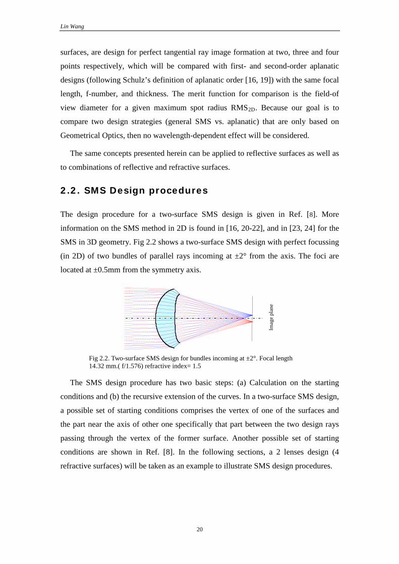
SMS in 3D geometry. Fig 2.2 shows a two-surface SMS design with perfect focussing
(in 2D) of two bundles of parallel rays incoming at ±2° from the axis. The foci are
located at ±0.5mm from the symmetry axis.
Fig 2.2. Two-surface SMS design for bundles incoming at ±2°. Focal length 14.32 mm.( f/1.576) refractive index= 1.5
The SMS design procedure has two basic steps: (a) Calculation on the starting
conditions and (b) the recursive extension of the curves. In a two-surface SMS design,
a possible set of starting conditions comprises the vertex of one of the surfaces and
the part near the axis of other one specifically that part between the two design rays
passing through the vertex of the former surface. Another possible set of starting
conditions are shown in Ref. [8]. In the following sections, a 2 lenses design (4
refractive surfaces) will be taken as an example to illustrate SMS design procedures.
Imag
e pl
ane

Chapter 2 SMS imaging design of rotational optics using meridian rays
21
2.2.1. Central conditions for SMS 3 and 4 surfaces
The SMS design procedure for more than 2 surfaces differs from the two-surface
one at the first step. In the four-surface case, the starting conditions include the parts
of the surfaces near the axis, which are calculated with Gaussian optics, but with the
additional condition that there are three or four rays connecting each of the design
points on the object with its corresponding image point (see Fig 2.3 and Fig 2.4). The
minimum initial part fulfilling this condition is selected. The remaining parts of the
curves are deleted.
Fig 2.3 Initial calculations for the three-surface SMS design.
In Fig 2.3 , 3 object points and 3 corresponding image points are selected to be
symmetrical to the central axis. The frontal surface of the first lens is given as a plane.
If we apply the central conditions given in Section 2.2.1, we can find that there is a
fast construction way to get central segments. If the connecting ray between object
point 1 and image point 1’ passes through the vertex of curve 3, we can construct
central segments in the following way:
(1) P1 can be selected freely on the frontal planar curve C1.
(2) Ray from object point 1 passes through P1, and be refracted. P2 is the then
selected along the refracted ray. The distance between P1 and P2 can be
determined based on the first lens’ thickness specification.
(3) Since the ray that passes through P2 should be refracted to P3, which is the vertex
of curve C2, we can then calculate normal vector on P2.
(4) Since P3 lies on the optical axis, its normal vector also follows the direction of
optical axis. The connecting ray coming from point P2 is then refracted at P3. P4

Lin Wang
22
can be selected along the refracted ray. The distance between P3 and P4 can also
be determined from the second lens’ thickness specification.
(5) Normal vector on P4 is calculated similarly as P2.
The above procedures can also be applied when object plane is at infinity.
Different selection of P1 gives different central segments, which are all solutions to
the central conditions.
If the frontal surface also needs to be designed, 4 connecting rays have to be
selected between 4 object points and their corresponding image points, as shown in
Fig 2.4. Then there is no fast construction way to get central segments. In this
situation, each one of the four rays (or their symmetric counterparts) crosses 2 of the 8
edges of the 4 curves A, B, C and D. Rays 1-1’ and 4-4’ are symmetric. The four
colored dots at the bottom edges of the curves indicate which design rays are passing
through them. There is at least one ray (the blue ray in the case of Fig 2.4) with a
single bottom edge point. If this is not so, then another four rays can be selected that
give smaller initial portions of curves A, B, C and D.
Fig 2.4. Initial calculations for the four-surface SMS design.
In order to express the above starting conditions in mathematics equations, we can
suppose that the central vertices are pre-fixed and central segments are represented by
spheres, whose radius curvatures are unknowns. From mathematical point of view, the
condition of 4 connecting rays between selected objects and images establishes 4
equations to 4 unknown central curvatures of spheres, as shown in equation system
(2.2). x1, x2, x3, x4 are positions of selected objects, which can be considered as
constant. x1*’, x2*’, x3*’, x4*’ are desired image points after ray-tracing through the
four optical surfaces.
1
Obj
ect p
lane
2
3
4
4’
3’
2’
1’
Imag
e pl
ane
A B C D
x x' α
β = −α

Chapter 2 SMS imaging design of rotational optics using meridian rays
23
1 1 2 3 4 1*
2 1 2 3 4 2*
3 1 2 3 4 3*
4 1 2 3 4 4*
'( , , , , ) ''( , , , , ) ''( , , , , ) ''( , , , , ) '
X x R R R R xX x R R R R xX x R R R R xX x R R R R x
====
(2.2)
However, Eq. (2.2) doesn’t describe sufficiently these connecting rays, because
these connecting rays have to follow a certain intersection conditions on optical
surfaces. We can suppose that the first connecting ray starts from point x1 and tilts an
angle α with respect to the optical axis, as shown in Fig 2.4. When central radii R1,
R2, R3, R4 are given, other 3 connecting rays can be determined based on the above
connecting conditions. Therefore, a more adequate description is given in equation
system (2.3).
1 1 2 3 4 1*
1 2 1 2 3 4 2*
1 2 3 1 2 3 4 3*
1 2 3 4 1 2 3 4 4*
'( , , , , , ) ''( , , , , , , ) ''( , , , , , , , ) ''( , , , , , , , , ) '
X x R R R R xX x x R R R R xX x x x R R R R xX x x x x R R R R x
αααα
==
==
(2.3)
Angle α gives another unknown, which has to fulfil the minimum initial part
condition. The minimum initial part condition can also be interpreted as the
symmetrical condition between the connecting ray 1and connecting rays 4, as shown
in Fig 2.4. However, even to the simplest case where all refractive surfaces are
spheres, analytical solutions to these 4 equations haven’t been found yet, due to the
nonlinearity of refraction laws introduced by each refractive surface during ray
tracing and the connection conditions between rays. We can use numerical
optimization method to solve equation system (3). The merit function for this example
is a combination of weighted functions, shown in equation (4). Table 2.1 gives an
example of how to solve equation system (3) with optimization method. The
maximum length column corresponds to the maximum size of four central segments.
In this example, it is reasonable to choose angle α as 6 degrees.
4
2 21 2 3 4 0 *
1
1( , , , , ) ( ) ( ' ')4central conditoins i i i
if R R R R w w x xα β α
=
= + + −∑ (2.4)

Lin Wang
24
Table 2.1. Optimization of angle α:
α (degree) Merit function Maximum length(mm) 0 0.00153189 0.679938 1 0.0021083 0.649351 2 0.00214073 0.618522 3 9.46362e-05 0.62093 4 4.32213e-06 0.569131 5 1.57261e-06 0.519057 6 1.56798e-06 0.473449 7 2.58076e-05 0.446901 8 0.00121638 0.397326 9 0.00240287 0.314328
2.2.2. Recursive SMS construction
Fig 2.5. SMS chain concept and SMS segment concept
Previous SMS 2D algorithms [16, 9] use "SMS chain” to construct curve’s profile.
The SMS chain concept is valid for 2 surfaces’ algorithm, because only previous
chain point is necessary for the new point calculation. When dealing with more than 2
surfaces, this concept becomes inapplicable because there is no clear SMS chain
appeared during the design process, as shown in Fig 2.5. To calculate a new curve
point with constant optical path length condition, a ray should be traced firstly
through the existing part of lens. Therefore, in each cycle, not only separate points,
but also the curve segment needs to be calculated out, so that new cycles can make
use of that calculated curve segment.
Then the generalized Cartesian Oval calculation requires to calculated several
points, through which a curve can be interpolated. When curve segment is small
enough, parabolic segment with few parameters is a good second order approximation
to the original segment. A parabolic segment can have several equivalent
representations, such as x polynomial representation and Bezier representation [28],
(a) SMS chain (b) SMS segment

Chapter 2 SMS imaging design of rotational optics using meridian rays
25
shown in Fig 2.6. C1 continuity between segments should be guaranteed on the
connection point to make whole curve smooth. Fig 2.6(a) shows that new segment is
represented by x polynomial with “α” as free parameter. The y axis of new parabolic
segment coincides with normal vector of previous end normal vector. Only a small
portion of parabola with size ∆S is taken as the new segment. In Fig 2.6(b), the
parabolic segment is represented by Bezier polynomial. Different from x polynomial
shown in Fig 2.6(a) where only central portion is utilized, Bezier polynomial can
represent any portion of parabola in a simple form. There are two degrees of freedom
in a Bezier polynomial representation, because control point P1 should lay on the
tangent plane of point P0, and point P2 should be selected to maintain a given size of
parabola.
Fig 2.6. Different representations of parabola
Because the x polynomial is not straightforward in representing a segment, it’s
convenient to change x polynomial to its equivalent Bezier Polynomial, as shown in
Fig 2.7. The parabolic segment is placed in the coordinate system, extended by the
normal vector and tangent vector of the end point of previous segment. Actually, x
polynomial representation can be treated as a special case of Bezier polynomial,
where x1 = ∆s/2 [36].
Fig 2.7. Bezier representation with 2 degrees of freedom
(a) x Polynomial (b) Bezier Polynomial

Lin Wang
26
With the small segment assumption, generalized Cartesian Oval calculation is
equivalent to the best fit problem of parabolic segment, so that constant optical path
length condition can be satisfied to the maximum extend. Considering that there are
only one or two parameters, we can trace a bundle of rays through the new parabolic
segment to the image plane. The free parameters of that parabolic segment are then
optimized, so that the merit function (RMS spot diameter) is minimized for the traced
meridian ray fan. Fig 2.8 shows a typical parametric distribution of RMS merit
function with respect to free parameters around the optimum position. The merit
function is more sensitive to the displacement of the control point P2, than to the
displacement of control point P1. Therefore, x polynomial at some circumstance can
provide fairly good approximation to the solution. However, in order to get the
closeness of approximation as high as possible in the SMS algorithms, we will always
use parabolic segment with 2 degrees of freedom.
Fig 2.8. landscape of merit function for one parabolic segment
Let’s go back to the 4 lens surface design example. The rest of the lens is
calculated in step (b) (SMS extension of the curves). As with any other SMS
extension, this step is characterized by a sequence of generalized Cartesian ovals
being calculated. In each of these generalized Cartesian oval calculations, the
trajectories of a small fan of rays are known when crossing all but one of the curves
(A, B, C, D). The portion of this last curve that is crossed by the fan can be calculated
by equating the optical path lengths. For instance, the rays reaching point 4’, below
the blue-colored ray of Fig 2.4, can be traced back through the surfaces B, C and D, as
shown in Fig 2.9(a). These rays should come from point 4. Consequently we can
calculate the red portion of curve A, as shown in Fig 2.9(a).

Chapter 2 SMS imaging design of rotational optics using meridian rays
27
Fig 2.9. SMS calculation of the remaining parts of the surfaces A, B, C and D.
Once this new portion has been calculated, at least one new fan of design rays is in
the same situation as before. In this case, this fan links points 3 and 3’ (see Fig 2.9b).
The rays issuing from 3 can be traced through the portion of curve A just calculated.
The rays of 3’ can be traced back through the curves C and D. Now we can calculate a
new portion of surface B as a generalized Cartesian oval. This procedure can be
repeated to calculate more portions of the curves (see Fig 2.9c). The order at which
each curve progresses is not necessarily the same during the iteration. Note that since
this case is symmetric, every time we calculate a new portion of a lens, its symmetric
counterpart is also calculated. As in any refractive Cartesian oval calculation, the
SMS extension procedure may give curves that do not represent physically possible
optical systems, although they fulfil the equality of optical path lengths between
corresponding points. In these cases, different sets of initial conditions must be
explored to find a feasible solution.
1
2
3
4
Obj
ect p
lane
Imag
e pl
ane
4’
3’
2’
1’
A B C D
4’
3’
2’
1’
A B C D
1
2
3
4
Obj
ect p
lane
Imag
e pl
ane
(a)
(b)
4’
3’
2’
1’
A B C D
1
3
4
Obj
ect p
lane
Imag
e pl
ane
(c)
2

Lin Wang
28
Fig 2.10 shows a four-surface SMS design formed by two lenses with initial
conditions of identity of the lens thicknesses and of both with the air space between
them. This design sharply focuses the bundle of incoming parallel rays with directions
±2° and ±6°, respectively at points ±0.3mm and ±0.9 mm off axis.
Fig 2.10. Four-surface SMS design for bundles at both ±2° and ±6°. Focal length 8.59 mm. (f/1.496). refractive index = 1.5.
2.3. Results and Analysis
Although SMS method provides an innovative constructive way to the original optical
design problem, the presented algorithm still subjects to instability problem. The
instability problem involves the range of parameters within which the SMS algorithm
can work properly, and the quality of constructed curves. The instability of SMS
algorithm can seriously affect the total design time and makes itself not suitable to be
embedded in an optimization process. We will examine this instability problem in
Section 2.3.1, and then analyse those stable designs in Section 2.3.2.
2.3.1. Instability analysis of SMS 3-surface designs
The instability problem occurs in both 3 surfaces and 4 surfaces SMS algorithms.
The most headache moment of developing an algorithm is not how to figure out the
problem when it doesn’t work at all, but when it works sometimes and doesn’t work
other times. The instability problem of current SMS algorithm results in bad RMS
performance and low quality of constructed curves.
Fig 2.11 is a SMS 3-surface design example with one planar frontal surface.
Object plane is placed at infinity. The central segments are obtained constructively as
described in Section 2.2.1. “x” coordinate of point P1 can be chosen freely on the
plane surface. Different “x” value corresponds to a different solution of the central
segments, as shown in Fig 2.12. And these central segments will lead to different
bending of lens after SMS construction, as shown in Fig 2.13.
Imag
e pl
ane

Chapter 2 SMS imaging design of rotational optics using meridian rays
29
Fig 2.11. Sketch of SMS 3-surface design. Designed object angles (00, ±90), focal length 9mm, vertices position from image plane (42,37,25,20)mm measured from the image plane.
Fig 2.12. Different central segments depending on the initial value of “x”: the central bending of the second lens is gradually changing with “x” value

Lin Wang
30
Fig 2.13. SMS construction from central segments with different initial “x” values
At the moment, there are no clear criteria to determine which “x” value gives
better optical performance than others before all the surfaces are constructed and ray-
traced. In this sense, although the SMS method presented above can generate easily
high order aspheres, the quality of generated curves has not been guaranteed, which
will lead to a tedious “try and error” process. An intuitive inspection of the curvature
distribution of curve segments also indicates that not all “x” value will result in
similar quality curves, as shown in Fig 2.14, where curves are represented in bright
colors and curvature are represented in gray color. High curvature value corresponds
to more bending, and vice versus. It can be seen in Fig 2.14 that the central big
segment is connected with small segments calculated in SMS construction process.
The connection however is smoother when “x” value is equal to 0.25mm. In the other
cases, there exist small or big “steps” at that connection point. If these curves are
going to be expanded in polynomial series, which is a standard form in imaging
analysis, it is obvious that discontinuity on the curvature distribution will cause severe
deviation in the following best fit process with polynomials.

Chapter 2 SMS imaging design of rotational optics using meridian rays
31
Fig 2.14. Comparison of curvature distributions on the second curve: at 0.25mm, the curvature distribution is much smoother than other “x” values. The shape increase of curvature at the edge corresponds to the caustics of rays happening at the edge of that segment.
Fig 2.15 gives the ray-tracing results of each solution. In this analysis, only
meridian rays from various incident angles are traced though each solution to compute
the blur spots radius on the image plane, which we call “RMS2D”. At 9 degrees, all
RMS2D distributions appear a local minimum, because the incoming rays have been
designed with the SMS process.
Fig 2.15. RMS2D distribution of different solutions. When “x” = 0.25mm, the RMS2D values are much lower compared with other solutions.
Results and inspections in Fig 2.14 and Fig 2.15 not only explain the “instability”
problem of the current SMS algorithm, but also indicate that there exists an optimum
solution within all possible solutions. It will be explained in the next chapter why
0.3mm 0.25mm 0.2mm 0.1mm
Connection point

Lin Wang
32
solution with “x” value equates 0.25mm can give much better results than other
solution.
2.3.2. SMS designs vs. Aplanatic designs
Let θ be a ray’s off-axis angle. We are going to compare several aplanatic designs
with equivalent SMS designs. In both cases we assume the object points to be at
infinity (i.e., parallel rays). To evaluate the imaging quality of a design we will use
the RMS spot radius functions RMS(θ)=RMS(P) and RMS2D(θ)=RMS2D(P), where P
is the image point of the bundle of parallel rays incoming at the direction angle θ.
Because all design rays are in the meridian plane, an SMS design of N surfaces will
have RMS2D(θi)=0 for N design directions θi, (assuming that a negligible
contribution of the initial parts of the four-surface SMS design, which is not
theoretically perfect). Then,
( )2D1
( ) ( )N
ii
RMS Aθ θ θ θ=
= −∏ (2.5)
As shown in ref [25], A(θ) is an arbitrary analytic function of θ which, in a first
approximation can be considered a constant function of θ (although the value of this
constant varies with different designs), i.e., RMS2D(θ) is approximated by the
absolute value of an N-degree polynomial. The ray tracing results of Fig 2.16 show
that this approximation is good in this case, and that the spot radius RMS2D(θ) is the
absolute value of a parabolic function of θ for small θ. Fig 2.16 left plots RMS(θ)
(dotted lines) and RMS2D(θ) (continuous) of three lenses with the same on-axis
thickness, the same focal length f=14.31mm, and the same f-number f/1.576. The
leftmost surface acts as stop surface. One of the lenses is designed for θi=±2º and
another for θi=±1º, while the last one is the aplanatic case, which can be seen as an
SMS case with its two off-axis directions become on-axis (θi→0°). The value of the
constant A turns out to be quite similar in all three cases. The lens profiles of the three
lenses considered in Fig 2.16 are very similar to the one shown in Fig 2.4(the
maximum deviation between curve profiles is less than 13 microns). These results are
similar to those shown in [8] and in [26].
The merit function for comparing these results is the field of view (FOV) diameter
for a given maximum RMS spot radius RMSM, i.e., the problem is to maximize the
FOV when the maximum allowable spot size in the FOV is limited to a given value

Chapter 2 SMS imaging design of rotational optics using meridian rays
33
(for instance, this RMSM can be the pixel radius of a detector to be placed at the focal
plane). Fig 2.16-left shows that no matter the value of RMSM, there is always an SMS
design with a wider range of incidence angles (i.e., a wider FOV) than the aplanatic
design of equal focal length and f-number. This best SMS design is the one having the
maximum allowable spot size at both normal incidence and the edge of the field. For
example, when the maximum RMS spot radius is RMSM≈11.1 µm, the SMS design
having the widest FOV diameter (which is ≈5.9º) is the one designed for incidence
angles θi=±2º. Included in this comparison is the SMS ±0º design, which is simply the
aplanatic design. Fig 2.16-right, shows the maximum RMS spot radius RMSM vs.
FOV diameter for the aplanatic case and for these SMS designs. This result does not,
however, prove that the present SMS designs reach the absolute maximum value of
that merit function.
Fig 2.16 also shows that RMS(θ) and RMS2D(θ) of these two-surface SMS designs
are quite similar, which means that the selection of the meridian ray bundles as design
rays gives good control of the function RMS(θ), i.e., of the RMS spot radius for all
the rays.
Fig 2.16. Continuous lines are for meridian rays, while dotted lines are for all rays. All the lenses have focal length 14.32mm and f/1.576. Left: RMS spot radius in microns. Two of the lenses are two-surface SMS designs for perfect meridian-ray imaging of rays incoming at ±1° and ±2° respectively. The third lens is an aplanatic design. Right: Maximum spot radius vs. the FOV diameter for aplanatic and SMS lenses of different design directions θ i.

Lin Wang
34
Fig 2.17. RMS spot radius in microns of a 3-surfaces SMS design for perfect imaging of incoming rays in directions ±3º and 0º. Refractive index at the image side is 1.5. The red dashed curve is the absolute value of the polynomial approximating the RMS spot radius (RMS2D(θ))
Fig 2.18. RMS spot radius of two designs with focal length 8.59 mm and f/1.496. Each design contains two lenses. One of the designs, that of Fig 2.10, is a four-surface SMS for perfect imaging of incoming rays in directions ±2° and ±6° respectively. The other design is second order aplanatic. Continuous lines consider only meridian rays, dotted lines considers all the rays.
Fig 2.18 shows the RMS spot radius RMS2D(θ) calculated by ray tracing of the
four-surface SMS design of Fig 2.10, as compared with a second order aplanatic
design with the same number of surfaces same thicknesses, and same f/1.496 and
focal length of 8.59 mm. Again, the second order aplanatic design can be viewed as
an SMS design at the limit of the four design directions becoming on-axis (θi→0°).
Although the design of Fig 2.10 shows equally spaced incoming directions
(θi= ±2º, ±4º), this is not necessary in an SMS design. Equally spacing θi gives
approximately a constant ripple of RMS2D(θ), as Fig 2.18 shows. When a maximum
spot radius ΡΜΣM is fixed, the constant ripple, constrained to RMS2D(θ) ≤ RMSM,
maximizes the angular field of view for the function RMS2D(θ). Fig 2.18 clearly
shows that the FOV corresponding to the function RMS2D(θ) of the SMS design is
wider than the FOV of the aplanatic case. Nevertheless, the function RMS(θ) (dotted
0
5
10
15
-10 -8 -6 -4 -2 0 2 4 6 8 10 Incidence angle (deg)
RMS
spot
radi
us (µ
m)
SMS ±2 and ±6 deg
2nd order aplanatic f# =1.496, focal length = 8.59 mm

Chapter 2 SMS imaging design of rotational optics using meridian rays
35
line in Fig 2.18) is not close to RMS2D(θ) in this four-surface designs, showing that
the selected design ray bundles give good control of the function RMS2D(θ) but not
good enough for the RMS spot radius of all the rays (RMS(θ)). The selection of the
design ray bundles for an optimum control of RMS(θ) is a subject of our present
research.
2.4. Conclusions
We have shown a new design strategy for imaging applications of the SMS method,
in which we choose as many couples of input and output meridian-ray bundles as
there are surfaces of the optical system to be designed. The SMS method ensures that
the input and output meridian-ray bundles become fully coupled by the optical system.
In the particular examples shown the input bundles are sets of parallel rays with
directions θi and the output bundles are their focal points. There exist “instability”
problem in the presented SMS algorithm. Curvature inspection and RMS2D
distribution analysis indicates that the curvature distribution is linked to the RMS2D
performance and there exist an optimum set of central curve segments.
In comparison with the aplanatic designs, once a maximum spot radius in the field
is fixed, the SMS design has a wider FOV (the FOV diameter of the SMS design is
1.42 times that of the equivalent aplanatic designs for the two-surface design). We
have also seen that aplanatic designs can be viewed as particular cases of SMS
designs when the design directions θi coincide with the optical axis. In the four-
surface SMS design case, we have shown that the selection of design rays among the
meridian rays of the FOV give good control of the image formation quality only for
meridian rays but not good enough to control of the remaining rays.
References
1. M. Born and E. Wolf, Principles of Optics, (Cambridge University Press, 1999).
2. R. Kingslake, Lens Design Fundamentals (Academic, New York, 1978).
3. W. J. Smith, Modern Optical Engineering, 3rd ed. (McGraw-Hill, 2000).
4. R. E. Fisher and B. Tadic-Galeb, Optical System Design (McGraw-Hill, 2000).
5. A. E. Conrady, Applied Optics and Optical Design, Part 1, New edition 1992 (Oxford University Press and Dover Publications, 1929).

Lin Wang
36
6. G. G. Slyusarev, in Aberration and Optical Design Theory, pp. 499–502, Adam Hilger, Techno House, Bristol (1984).
7. G. W. Forbes, "Shape specification for axially symmetric optical surfaces," Opt. Express 15, 5218-5226 (2007) http://www.opticsinfobase.org/abstract.cfm?URI=oe-15-8-5218
8. P. Benítez and J. C. Miñano, "Ultra high-numerical-aperture imaging concentrator," J. Opt. Soc. Am. A 14, 1988-1997 (1997) http://www.opticsinfobase.org/abstract.cfm?URI=josaa-14-8-1988
9. K. Schwarzschild, Astronomische Mitteilungen der Königlichen Sternwarte zu Göttingen 10, 3 (1905), Reprinted: Selected Papers on Astronomical Optics, SPIE Milestone Ser. 73, 3 (1993).
10. G.D. Wassermann and E. Wolf, “On the Theory of Aplanatic Aspheric Systems,” Proc. Phys. Soc. B 62, 2-8 (1949)
11. W.T. Welford, “Aplanatism and Isoplanatism,” Progress in Optics XIII, 267-293, (1976)
12. L. Mertz, “Geometrical design for aspheric reflecting surfaces,” Appl. Opt. 18, 4182-4186 (1979).
13. L. Mertz, “Aspheric potpourri,” Appl. Opt. 20, 1127-1131 (1981).
14. D. Lynden-Bell, “Exact Optics: A Unification of Optical Telescope Design,” MNRAS 334, 787-796 (2002).
15. R.V. Willstrop, D. Lynden-Bell, “Exact Optics — II. Exploration of Designs On- and Off-Axis,” MNRAS 342, 33-49 (2003).
16. R. Winston, J.C. Miñano, P. Benítez, Nonimaging Optics, (Academic Press, New York, 2005)
17. M. Mansuripur, Classical Optics and its Applications (Cambridge University Press, Cambridge, 2002) p. 16
18. G. Schulz, Higher order aplanatism, Opt. Commun. 41, pp. 315–319 (1982).
19. G. Schulz, Aspheric surfaces, In: E. Wolf, (Ed.), Progress in Optics, 25, 1988, pp. 349–415
20. J. C. Miñano and J. C. González, "New method of design of nonimaging concentrators," Appl. Opt. 31, 3051-3060 (1992) http://www.opticsinfobase.org/abstract.cfm?URI=ao-31-16-3051
21. J. C. Miñano, P. Benítez, and J. C. González, "RX: a nonimaging concentrator," Appl. Opt. 34, 2226-2235 (1995) http://www.opticsinfobase.org/abstract.cfm?URI=ao-34-13-2226
22. J. C. Miñano, J. C. González, and P. Benítez, "A high-gain, compact, nonimaging concentrator: RXI," Appl. Opt. 34, 7850-7856 (1995). http://www.opticsinfobase.org/abstract.cfm?URI=ao-34-34-7850
23. P. Benítez, J.C. Miñano, J. Blen, R. Mohedano, J. Chaves, O. Dross, M. Hernández, J. Alvarez, W. Falicoff. “SMS Design Method in 3D Geometry: Examples and Applications,” Proc. SPIE 5185, 18-29 (2003).
24. J. Chaves, Introduction to Nonimaging Optics, (CRC Press, Boca Ratón, 2008).
25. F. Muñoz. Doctoral Thesis “Sistemas ópticos avanzados de gran compactibilidad con aplicaciones en formación de imagen y en iluminación” (2004).
26. N. Shatz and J. Bortz, “Optimized image-forming cemented-doublet concentrator,” Proc. SPIE, 5942, 59420G (2005).
27. José Blen Flores, Doctoral Thesis “Design of multiple free-form optical surfaces in 3D” 2007.
28. Les Piegl, Wayne Tiller, the Nurbs Book, (Springer 2nd edition 1997).

Lin Wang
37
Chapter 3. Improved SMS algorithms and parametric optimization
3.1. Introduction
Classic optical design methods are developed mainly from paraxial optics [1, 2].
Starting from a paraxial initial guess, multi-parametric optimization techniques are
then used to maximize the image quality for all fields of view. This classical design
strategy is very simple, but depends heavily on multi-parametric optimization
techniques and the closeness of initial guess to the optimum solution. If the initial
design is far from the optimum point, it is most likely that either optimizer would fail
to find useful solutions, or designers need to spend long hours to improve their initial
guesses. In order to obtain good image quality over all fields of view, the
Simultaneous Multiple Surfaces (SMS) method sets up the problem in a different way:
by perfectly controlling selected ray-bundles, a partial control over all the rays in the
phase space can be obtained. In a rotational symmetric system, SMS design procedure
involves simultaneous calculation of N rotational surfaces for given N uni-parametric
ray-bundles.
The Simultaneous Multiple Surfaces (SMS) method is a direct construction
method for selected ray-bundles, meridian or skew ray-bundles. The SMS method
was developed as a design method in Non-imaging Optics during the 90s [3-6], where
the imaging formation is not required. A famous theorem in Non-imaging optics is the
edge-ray theorem, which states that all rays will be transferred to the target, if the
edge-rays in phase space are coupled to the edge rays of the target. Therefore, SMS
method in the beginning only used edge-rays from light sources like the Sun or LEDs.

Chapter 3 Improved SMS algorithms and parametric optimization
38
With the development of SMS methods from 2 surfaces to 4 surfaces, it has been
found that by selecting more ray-bundles (N>2) from the phase space and designing
with SMS method, image quality is greatly improved. Research results shown in
Chapter 2 demonstrate that SMS method is superior to aplanatic design method in
controlling non-paraxial rays [6,7].
Selection of ray-bundles, meridian or skew ray-bundles, should vary from one
design to another, according to the size and shape of interested fields of view. There
have already been several applications of SMS methods to imaging optics [6-11]. In
ref [6], 2 meridian ray-bundles (2M) were designed to achieve high numerical
aperture and in ref [9], 3 meridian ray-bundles (3M) SMS design helped to achieve a
wide field of view. In Ref [10], 2 rotational mirrors were designed with 2 symmetric
skew ray-bundles (2S). Distortion added by these 2 mirrors was below 1%. Good
selections of ray-bundles in above cases have proven to be effective in the search for
good performance initial designs. Currently, for 3 surfaces SMS design, only meridian
ray-bundles can be selected in the phase space. This can limit the search space for
good initial designs, because our final goal is to acquire a good control over both
meridian rays and skew rays.
3.2. Phase space sampling
When considering all the rays in the phase space, perfect imaging of all object
points is not possible, because it’s limited by design freedoms. The idea of SMS
method is to make use of design freedoms to perfectly control a selection or a
sampling of ray-bundles, e.g. those rays that emanate from several selected object
points. Other non-selected rays can be considered in the phase space to have a certain
deviation distance from those selected rays. As an example, a Cartesian Oval is
calculated to transform a parallel wave-front into a spherical wave-front, as shown in
Fig 3.1. For 00 object angle, aberrations of all types have been corrected. For off-axis
object angles, it is typical to obtain the function of the RMS deviation of the impact of
the rays is a monotonic function as the one shown in Fig 3.1(b).

Lin Wang
39
Fig 3.1. The sketch of (a) a Cartesian Oval with (b) its RMS distribution for object angle θ
Fig 3.2 shows 2 types of ray-bundles selections suitable for simultaneous 3
surfaces calculation. In Fig 1a, y-z plane is considered as meridian plane. An object is
seen from a pin hole which locates at the y’ axis of the entrance pupil plane. The pin-
hole can move freely along that y’ axis. In Fig 3.2(a), 3 object points M1, M2 and M3
are placed equal-spaced along the y axis. Therefore, rays coming from those 3 object
points to the pin hole are all meridian rays. By moving the position of the pin hole
along the y’ axis, 3 meridian ray-bundles (3M) from the 3 meridian object points can
be defined. In Fig 3.2(b), object point M1 is placed on y-axis, and another 2 object
points S2 and S3 are placed symmetrically about y axis. Ray from M1 to pin hole is a
meridian ray and rays from object points S2 and S3 are skew rays. Moving pin-hole
position will therefore define 1 meridian ray-bundle and 2 symmetric skew ray-
bundles (1M-2S).
(a) (b)
Fig 3.2. Samplings in phase space for a rectangular object. (a) 3 meridian ray-bundles sampling; (b) 1 meridian 2 skew ray-bundles sampling.
The selection of meridian rays is straightforward, since these rays should be
contained in the meridian plane. The selection of skew rays is more complicate,
because any ray not in the meridian plane is a skew ray. The skew rays selection for
Image plane
θ = 00
(a)
RMS
θ (b)

Chapter 3 Improved SMS algorithms and parametric optimization
40
object point S2 shown in Fig 3.2(b) is a simplified case when these skew rays lie in a
skew plane. In order to have a clear view of ray selection, it’s convenient to plot these
selected ray-bundles in the top view, as shown in Fig 3.3. Point “P” on the entrance
pupil moves from center to the positive side of axis Y’, defining a set of meridian rays
shown in Fig 3.3(a) and Fig 3.3(b). Taking into account the rotational symmetry of
the optical system, the other unselected meridian rays shown in Fig 3.3(c) will also be
designed.
Fig 3.3. Perspective and top view of object plane for 3M sampling
Fig 3.4(a) gives the top view of a 1M-2S sampling. Selected skew rays from
object point S2 and S3 lie in a skew plane with angle ±α0 respecting the meridian
plane. When 3 object points M1, S2, S3 have the same distance to the object center, as
shown in Fig 3.4(b), these 3 object points are then identical due to the rotational
symmetry of system, and we can plot all selected rays for each object point.
(a) Perspective view
M2
Ray-cone defined by entrance pupil
Object plane
Chief ray
(b) Top view
Y
X
M3
M1
M2
Object plane
X
Y
(c) Top view
Y
X
M3
M1
M2
Object plane
Selected rays
Selected
Meridian
rays
Un-selected meridian rays

Lin Wang
41
Fig 3.4. 1M-2S sampling. (a) Selected ray-bundles (b) When 3 object points have the same distance to the object center.
When angle α0 is close to 0 degree, 1M-2S type sampling converges to 2M type
sampling. A direct guess indicates that the optimum value of angle α should be
around 600, so that selected rays can distribute uniformly in the object space.
From the pin-hole point of view, all the rays from object points to this pin-hole
form a rectangular or circular cone, depending on the shape of the object. A better
sampling of this cone of rays should be represented by rays distributed more
uniformly in this cone. In this sense, 1M-2S ray-bundles seem to provide a better
sampling of all rays than 3M ray-bundles.
In this work, SMS method is further extended by designing 3 rotational surfaces
with 1 meridian ray-bundle and 2 symmetric skew ray-bundles (SMS 1M-2S). As a
comparison of image forming ability, another design is realized with 3 meridian ray-
bundles (SMS 3M).
3.3. Improved SMS algorithms
In Chapter 2, we have set up an equation system to determine the shape of the
central segments, as shown in Eq. (3.1). This equation system formulates the
condition that all cutting rays from their object points should arrive to their
corresponding image points. However, solution to this equation system depends
heavily on the initial value, as shown in Fig 3.5. A bad choice of the initial value will
lead to instability or “bad quality” of constructed curves with the SMS construction.
Because real ray-trace, not paraxial ray-trace, is required to be performed through
(a) Top view
Y
X
S3
M1
S2 Object plane
Selected
Meridian
rays
Selected Skew rays
(b) Top view
Y
X
S3
M1
S2 Object plane
α0
−α0
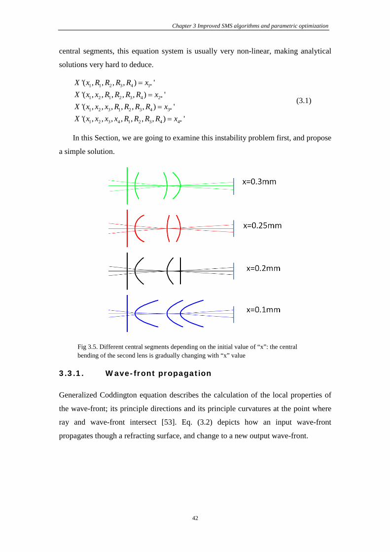
Chapter 3 Improved SMS algorithms and parametric optimization
42
central segments, this equation system is usually very non-linear, making analytical
solutions very hard to deduce.
1 1 2 3 4 1*
1 2 1 2 3 4 2*
1 2 3 1 2 3 4 3*
1 2 3 4 1 2 3 4 4*
'( , , , , ) ''( , , , , , ) ''( , , , , , , ) ''( , , , , , , , ) '
X x R R R R xX x x R R R R xX x x x R R R R xX x x x x R R R R x
==
==
(3.1)
In this Section, we are going to examine this instability problem first, and propose
a simple solution.
Fig 3.5. Different central segments depending on the initial value of “x”: the central bending of the second lens is gradually changing with “x” value
3.3.1. Wave-front propagation
Generalized Coddington equation describes the calculation of the local properties of
the wave-front; its principle directions and its principle curvatures at the point where
ray and wave-front intersect [53]. Eq. (3.2) depicts how an input wave-front
propagates though a refracting surface, and change to a new output wave-front.

Lin Wang
43
2212
12
2212
2 1
coscos'
coscos'
coscos'
cos cos
ir
q q sq
ir
s
ir
p p sp
r i
nn
nn
nn
n n
θθ γρ ρ ρ
θθ γσ σ σ
θθ γρ ρ ρ
γ θ θ
= +
= + = +
= −
(3.2)
Where n1 and n2 are refractive indices before and after refraction; θi and θr are the
incident angle and exit angle between the ray and the normal vector of the refracting
surface at the intersection point; p and q are two perpendicular directions on the
tangent plane of the intersection point. That’s to say, when dealing with input and
output wave-front, the tangent plane is on the wave-front; while for the refracting
surface, a subscript “s” is used, which indicates that the tangent plane is on that
refracting surface. Direction p also lies in the plane determined by the surface normal
and incident ray.
With the help of these notations, ρ'p and ρ'q give the curvature radius of output
wave-front in the p and q direction. When these two perpendicular directions are not
the principle directions, one can also obtain a “torsion” σ corresponding to these two
perpendicular directions.
Now we are going to analyze the meridian wave-front propagation for those
central segments in Fig 3.5. The object wave-fronts are three parallel planes,
corresponding to objects located at infinitive. After propagation through the central
segments, the output wave-fronts are displayed in Fig 3.6. As it can be seen, the off-
axis image point is changing with the initial value “x” from positions before image
plane to positions after the image plane. When “x” equates 0.25mm, the off-axis
image point coincides with the desired image plane. That explains the appearance of
C2 discontinuities (curvature discontinuities) at the joint positions between the central
segments and the segments calculated with SMS method (or SMS segments), when x
is not equal to 0.25mm. Because each SMS segment is designed to have the image
wave-front centered at its corresponding image point, but central segments in many
cases don’t fulfill that condition, causing this C2 discontinuity problem. This analysis
also provides an efficient way to eliminate these discontinuities that we are going to
present in the following sections.
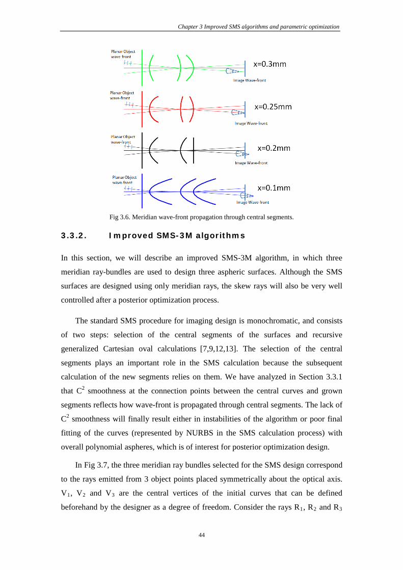
Chapter 3 Improved SMS algorithms and parametric optimization
44
Fig 3.6. Meridian wave-front propagation through central segments.
3.3.2. Improved SMS-3M algorithms
In this section, we will describe an improved SMS-3M algorithm, in which three
meridian ray-bundles are used to design three aspheric surfaces. Although the SMS
surfaces are designed using only meridian rays, the skew rays will also be very well
controlled after a posterior optimization process.
The standard SMS procedure for imaging design is monochromatic, and consists
of two steps: selection of the central segments of the surfaces and recursive
generalized Cartesian oval calculations [7,9,12,13]. The selection of the central
segments plays an important role in the SMS calculation because the subsequent
calculation of the new segments relies on them. We have analyzed in Section 3.3.1
that C2 smoothness at the connection points between the central curves and grown
segments reflects how wave-front is propagated through central segments. The lack of
C2 smoothness will finally result either in instabilities of the algorithm or poor final
fitting of the curves (represented by NURBS in the SMS calculation process) with
overall polynomial aspheres, which is of interest for posterior optimization design.
In Fig 3.7, the three meridian ray bundles selected for the SMS design correspond
to the rays emitted from 3 object points placed symmetrically about the optical axis.
V1, V2 and V3 are the central vertices of the initial curves that can be defined
beforehand by the designer as a degree of freedom. Consider the rays R1, R2 and R3

Lin Wang
45
shown in Fig 3.7, which all pass through the vertex of Curve 2: V2. R2 is the on-axis
ray emitted from the on-axis point Obj2 to reach its on-axis image point Img2. R1 is
emitted from an off-axis point Obj1 to reach its prescribed off-axis image point Img1
and R3 is its symmetrical counterpart.
Fig 3.7. Ray trajectories from the design object points to their corresponding image points used to design the central segments.
The trajectory of R2 from Obj2 to Img2 is guaranteed by normal incidence on all
surfaces. The condition that R1 emitted from Obj1 reaches Img1 sets up a relationship
between the slopes of Curve 1 and Curve 2 on their rims. Furthermore, the conditions
of C2 smoothness at these edge points set up a second constraint on the curvatures of
Curve 1 and Curve 2 on their rims. This second constraint is obtained by computing
the propagation using a generalized ray-tracing [14] of the meridian curvature of the
wave-fronts around R1 and forcing the center of curvature of that wave-front to
coincide with Img1. Eq. (3.3) is exactly the first equation of Eq. (3.2), which
establishes the relationship between the radius curvature of the incoming wave-front
ρi along a meridian ray, the radius curvature of the outgoing wave-front ρr and the
curvature of the intersected curve ρc. Angles αi and αr are incident and refracted
angles with respect to the normal. A similar law for reflective surface can be obtained
by changing nr to −ni in Eq. (3.3). Since there are two conditions to be fulfilled, two
degrees of freedom are needed, which means that Curves 1 and 3 can be represented,
for instance, as spheres, the two radii being calculated with these conditions. The
solution is in general not unique. Different solutions usually represent initial curves
with concave or convex shapes, which lead to different families of optical designs.
2 2cos ( cos cos )cosi i i i r rr r
i r c
n n nnα α ααρ ρ ρ
−− = (3.3)

Chapter 3 Improved SMS algorithms and parametric optimization
46
Once these central segments are selected, the following steps for progressing them
from center to the rim of the full aperture lenses are the SMS construction [10], as
explicated in Fig 3.8:
Fig 3.8. Steps of SMS construction
(a) Segment 1 of Curve 2 is calculated as a generalized Cartesian Oval to transform spherical wave-front from Object 2 to spherical wave-front of Image 2;
(b) Segment 2 of Curve 1 is constructed through calculated Segment 1, and transform spherical wave-front from Object 3 to spherical wave-front of Image 3;
(c) Segment 3 of Curve 3 is calculated through calculated Segment 1 and Segment 2;
(d) Repeat the above process.
The above processes can be also applied to transformation of wave-fronts in a general form.
3.3.3. Improved SMS-1M2S algorithm
SMS-1M2S algorithm is an extension to previous SMS 2S algorithm. Detailed SMS
2S algorithm can be found in ref [10]. Different from SMS 2S algorithm where
central curves were not necessary in the design, SMS 1M-2S algorithm needs central
curves for further SMS construction. Similar to SMS 3M algorithm where a 2D wave-
front criteria for meridian ray-bundles is proposed, a wave-front criteria is presented
here for 1 meridian and 2 skew ray-bundles.
In Fig 3.9(a), 3 object points M, S1, S2 are selected in the object plane. The YZ
plane is defined as the meridian plane. M is selected on the Y axis, and S1 and S2 are
symmetrical to the meridian plane. V1, V2, V3 are 3 central vertexes of initial surfaces,
which can be defined loosely from mechanical or optical requirements. 3 chief rays

Lin Wang
47
from 3 object points all pass through point V2, center of Surface 2, making
themselves meridian rays. Skew ray-bundle emanated from skew object points S1
situates in a skew plane which contains the chief ray, but has an angle α from the
meridian plane (α≠0); skew ray-bundle around chief ray of S2 in another skew plane
with -α angle to the meridian plane. In this way, selected ray-bundles for point S1 and
S2 are all skew rays except the first ray.
Fig 3.9. C2 continuous condition for 1M-2S central curves. (a) 3 chief rays pass through vertex V2 of S2; (b) meridian wave-front transformation; (c) 2 skew wave-fronts transformation; (d) (special case) transformation of a spherical object wave-front to a spherical image wave-front.
The C2 continuous condition requires that wave-fronts formed by selected
meridian and skew ray-bundles, close to chief rays in object space, should be
(a)
(b)
(c)
(d)

Chapter 3 Improved SMS algorithms and parametric optimization
48
transformed into its corresponding spherical image wave-fronts through this rotational
optical system, as shown in Fig 3.9(b) and Fig 3.9(c). The propagation of wave-fronts
through optical surfaces can be calculated analytically with generalized Coddington
equations (3.2).
In the following, we are going to consider the case when selected object points S1,
S2, and M have the same distance to the central axis, or 3 chief rays are identical. The
propagation of wave-front is illustrated in Fig 3.9(d). The exit image wave-front has
one meridian curvature km and one skew curvature ks, corresponding to selected
meridian and skew ray-bundles. In a rotational optical system, km is always one
principle curvature, and we suppose kq to be another principle curvature. From
Euler’s theorem, their relations are given in Eq. (3.4), where θ is the angle between
the skew plane containing the output skew ray-bundle and the meridian plane.
2 2cos sins m pk k kθ θ= + (3.4)
In order to achieve perfect imaging, the exit image wave-front should be spherical
centered at the desired image point S1’, S2’ and M’. Therefore, kp should be equal to
km in equation (3.4), and we can deduce that ks is always equal to km independent of
the angle α. Starting from initial surfaces that give spherical image wave-front, skew
ray-bundles can be selected in any direction, without violating the C2 continuous
condition at the connecting point. Once initial curves are obtained, SMS construction
can be started in the following order:
1. Skew ray-bundles are used to construct Surface 1 and Surface 2 at the same time,
which constant optical path length and conservation of skewness condition [10];
2. Meridian ray-bundle is used to construct Surface 3 with constant optical path
length condition;
3. Repeat the above process until aperture requirements are fulfilled.
3.4. A simple objective design example
Table 3.1. Optical parameters Focal Length F# Field of view Refractive index Lens’ surfaces
9mm 2 ±150 1.5 1 Frontal planar surface 3 aspherical surfaces
Parameters of objective lens are listed in table 3.1. Because our goal is to compare
two design strategies (SMS 1M-2S vs. SMS 3M) that are only based on Geometrical
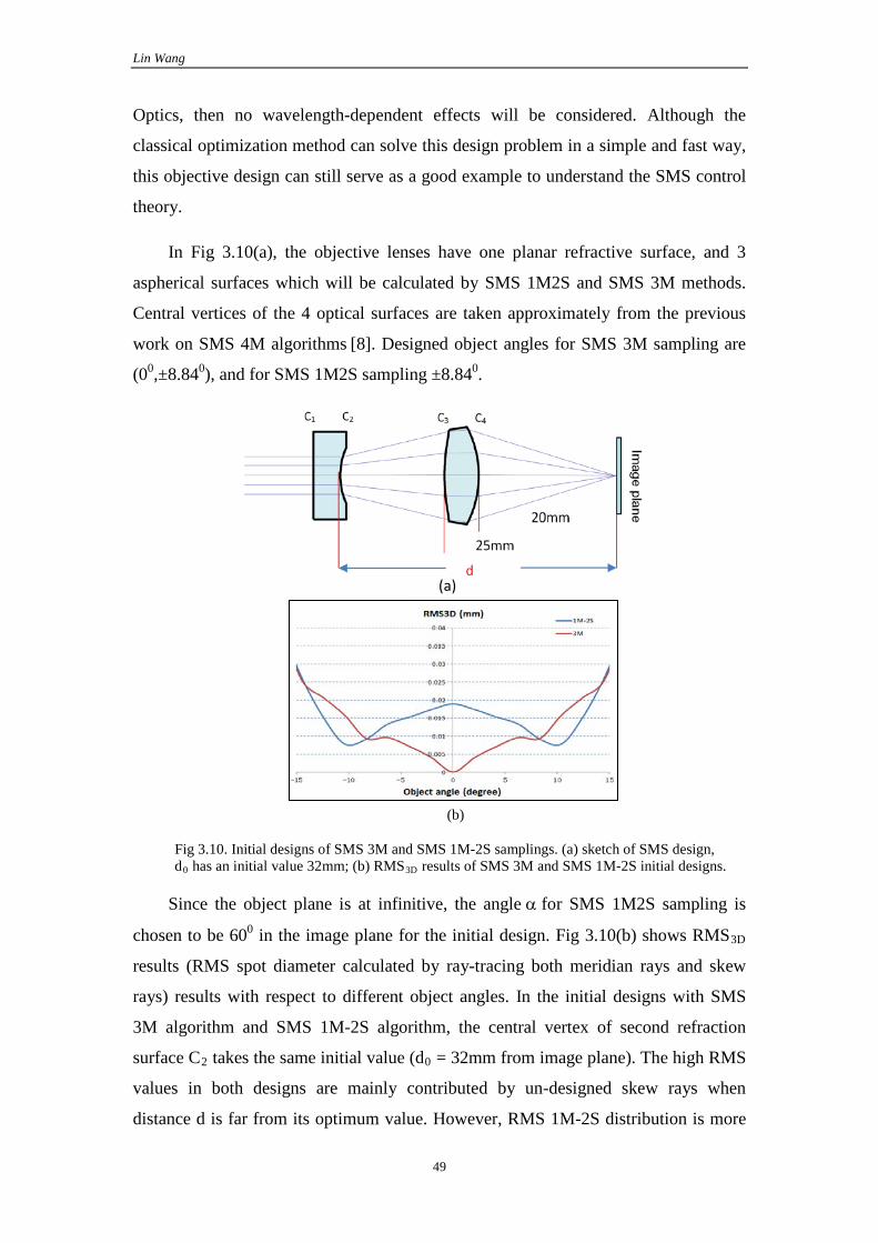
Lin Wang
49
Optics, then no wavelength-dependent effects will be considered. Although the
classical optimization method can solve this design problem in a simple and fast way,
this objective design can still serve as a good example to understand the SMS control
theory.
In Fig 3.10(a), the objective lenses have one planar refractive surface, and 3
aspherical surfaces which will be calculated by SMS 1M2S and SMS 3M methods.
Central vertices of the 4 optical surfaces are taken approximately from the previous
work on SMS 4M algorithms [8]. Designed object angles for SMS 3M sampling are
(00,±8.840), and for SMS 1M2S sampling ±8.840.
Fig 3.10. Initial designs of SMS 3M and SMS 1M-2S samplings. (a) sketch of SMS design, d0 has an initial value 32mm; (b) RMS3D results of SMS 3M and SMS 1M-2S initial designs.
Since the object plane is at infinitive, the angle α for SMS 1M2S sampling is
chosen to be 600 in the image plane for the initial design. Fig 3.10(b) shows RMS3D
results (RMS spot diameter calculated by ray-tracing both meridian rays and skew
rays) results with respect to different object angles. In the initial designs with SMS
3M algorithm and SMS 1M-2S algorithm, the central vertex of second refraction
surface C2 takes the same initial value (d0 = 32mm from image plane). The high RMS
values in both designs are mainly contributed by un-designed skew rays when
distance d is far from its optimum value. However, RMS 1M-2S distribution is more
(a)
(b)

Chapter 3 Improved SMS algorithms and parametric optimization
50
uniform than RMS 3M distribution over all fields of view.
Then, the vertex position of the second refractive surface C2 is optimized to
minimize largest RMS spot diameter (RMS3D) over all fields of view. During this one
parameter optimization, SMS 1M-2S and SMS 3M algorithms are repeated
respectively for each vertex position of C2. Fig 3.11 gives how the merit function
varies with respect to different value of d0.
Fig 3.11. C2 Vertex position optimization and comparison of RMS3D results. (a)RMS3D merit function with respect to C2 vertex position; (b) RMS3D distribution over all fields of view at each optimum vertex position.
Fig 3.11(a) shows that although the initial design is relatively far from the
optimum position, each merit function has only one minimum position which can be
easily found by any optimizer. Comparing RMS3D results in Fig 3.11(b), it can be
seen that the optimum SMS 1M-2S design has a more uniform RMS3D distribution
than SMS 3M design. This is due to the fact that three ray-bundles selected by SMS
1M-2S algorithm are distributed more uniformly in the phase space, therefore enable
a balanced control over all the other rays. The power of control over large fields of
views (>10 degree) is very similar for both optimum designs. However, due to lack of
(a)
(b)

Lin Wang
51
control over on-axis rays, SMS 1M-2S algorithm is less effective in minimization of
RMS spot size for the central field of view.
In the previous optimization process, angle α for SMS 1M-2S design is set to be
600, and an optimum position d = 37mm has been found as shown in Fig 3.11(a). Fig
3.12 shows RMS3D results of designs with different angle α (300, 450, 600, 700 and
800) at the optimum C2 vertex position (d = 37mm). In general, their RMS3D
distributions are very similar to each other in both trend and magnitude; however,
α equaling to 600 gives a bit better result than other angles.
Fig 3.12. Comparison of RMS3D distributions for different angle α.
To further understand the power of control over skew rays in both designs,
distribution of RMS spot diameters over different skew ray-bundles (RMS (γ,β)) are
calculated, as shown in Fig 3.13(a). “r” represents the radial position of an object
point in the object plane; when object plane is placed at infinity, object position “r”
becomes to be object angle “γ”. “β” represents the radial angle about axis Y in the
entrance pupil. γ and β together define a bundle of rays to be ray-traced to the image
plane. In Fig 3.13(b), Fig 3.13(c) and Fig 3.13(d), we can find 3 lowest RMS diameter
spot (< 0.2µm) in each RMS(γ, β) distribution. These lowest spots correspond to the
selected ray-bundles for SMS construction. Therefore both algorithms (SMS 3M and
SMS 1M-2S) have successfully control the designed ray-bundles. Also, central RMS
distribution of the SMS 3M design has smaller values than those of SMS 1M-2S
designs. Integration of RMS (γ,β) over radial angle β will lead to results shown in Fig
3.12.

Chapter 3 Improved SMS algorithms and parametric optimization
52
Fig 3.13. RMS(γ, β) distribution: RMS spot diameter calculated by tracing rays defined by parameters γ and β.
3.5. Conclusion
In this work, we have improved the SMS-3M algorithm and SMS 1M-2S algorithm
for selected ray-bundles. To provide a better selection of central curves for further
SMS construction, the central segments have to fulfill C2 continuous condition at the
connection points with the later SMS constructed segments. This addition condition
removes many unstable solutions mentioned in Chapter 2.
The SMS 1M-2S and SMS 3M algorithms are then applied to a monochromatic
objective design to compare their control capability over all the rays in the phase
space, or their imaging ability. By the vertex optimization of the second refractive
surface, which is a one parameter optimization, largest RMS3D in all fields of view
has dropped below 4µm, and RMS spot diameters for selected ray-bundles are well
d) SMS 1M-2S, α = 600
b) SMS 3M a) RMS(γ, β) ray-tracing
c) SMS 1M-2S, α = 300

Lin Wang
53
controlled below 0.2µm. Results have shown that by selecting ray-bundles which
spread uniformly in phase space, SMS 1M-2S design has a more uniform RMS3D
distribution before and after vertex optimization. However compared to SMS 3M
design, it still has less control of RMS spot size over all fields of view, especially the
center field of view. Also, different selection of angle α in the SMS 1M-2S algorithm
does not change significantly the RMS3D distribution; α = 600 gives a bit better choice
than other angles.
References
1. M. Born and E. Wolf, Principles of Optics, (Cambridge University Press, 1999).
2. R. K. Luneburg, Mathematical Theory of Optics, (University of California Press , 1964).
3. R.Winston, J.C. Miñano, P. P. Benítez, with contributions of N. Shatz, J. Bortz, Nonimaging Optics, (Academic Press Elsevier, 2004), Chap. 8.
4. Chaves, J., Introduction to Nonimaging Optics, (CRC Press, 2008).
5. Pablo Benítez, Juan C. Miñano, José Blen, Rubén Mohedano, Júlio Chaves, Oliver Dross, Maikel Hernández, and Waqidi Falicoff, “Simultaneous multiple surface optical design method in three dimensions,” Opt. Eng. 43, 1489 (2004).
6. P. Benítez and J. C. Miñano, "Ultra high-numerical-aperture imaging concentrator," J. Opt. Soc. Am. A , Vol 14 (1997).
7. J. C. Miñano, P. Benítez, W. Lin, J. Infante, F. Muñoz, and A. Santamaría, “An application of the SMS method for imaging designs,” Opt. Express 17(26), 24036–24044 (2009).
8. Miñano, J.C., Benítez, P., Wang Lin,, Muñoz, F., Infante, J., Santamaría, A., “Overview of the SMS design method applied to imaging optics”, Proc. SPIE 7429, 74290C (2009).
9. Jose M. Infante Herrero, Fernando Muñoz, Pablo Benitez, Juan Carlos Miñano, Wang Lin, Juan Vilaplana, Guillermo Biot, Marta de la Fuente “Novel fast catadioptric objective with wide field of view”, Proc. SPIE 7787, 778704 (2010).
10. F. Muñoz, P. Benítez, and J. C. Miñano “High-order aspherics: the SMS nonimaging design method applied to imaging optics”, Proc. SPIE 7061, 70610G (2008).
11. Fernando Muñoz Doctoral Disertation “Sistemas ópticos avanzados de gran compactibiliad con aplicaciones en formación de imagen y en iluminación” UPM, Madrid (2004)
12. Wang Lin, Pablo Benitez, Juan Carlos Miñano,Jose M. Infante Herrero, Guillermo Biot, “Progress in the SMS design method for imaging optics,” Proc. SPIE 8129, 8128-14 (2011).
13. Wang Lin, Pablo Benitez, Juan Carlos Miñano,Jose M. Infante Herrero, Marta de la Fuente, Guillermo Biot, “Ultra-compact SWIR telephoto lens design with SMS method,” Proc. SPIE 8129, 8129-16 (2011).
14. Orestes N. Stavroudis, The mathematics of geometrical and physical optics, (Wiley-VCH, 2006).

Chapter 4 Ultra-Compact SWIR telephoto camera design
54
Chapter 4. Ultra-compact SWIR telephoto camera design
4.1. Design background
The SWIR stands for Short Wave length Infrared, which ranges between 0.9µm
and 1.7µm. Although light in the shortwave infrared region is not visible to the eye,
this light interacts with objects in a similar manner as visible wavelengths. That is,
SWIR light is reflective light; it bounces off of objects much like visible light. As a
result of its reflective nature, SWIR light has shadows and contrast in its imagery [1].
Moreover, SWIR band has many amazing properties which visible band doesn’t
possess. Firstly, SWIR band light can penetrate through visible obstacles like haze,
fog, silicon glass and plastics. Secondly, an atmospheric phenomenon called night sky
radiance emits five to seven times more illumination than starlight, nearly all of it in
the SWIR wavelengths. A night vision device that uses the SWIR band light can have
clearer images even in a starless night, as shown in Fig 4.1 [1].

Lin Wang
55
Fig 4.1. Images taken by visible band camera and SWIR band camera. (a) Visible camera can barely see a hotel in a foggy day by; (b) SWIR camera can clearly see the hotel in the same day (c) Visible camera can hardly see the road condition in the night; (d) SWIR camera can see clearly the road condition.
Although these remarkable properties of the SWIR band had already been noticed,
widely utilization of SWIR band was not possible due to the lack of proper sensor that
can operate under room temperature without cooling system. Recently developed
InGaAs sensor finally overcomes this practical limitation [1-4]. Fig 4.2 shows two
series of InGaAs SWIR camera, which have high resolution and compact module.
Working temperature of these cameras normally ranges from -250 to 450. Some
cameras can even operate between -400 and 700 [1].
Fig 4.2. Compact and high resolution SWIR cameras.
(a) 640×512 pixel format (b) 1280×1024 pixel format
(a) Visible (b) SWIR
(c) Visible (d) SWIR

Chapter 4 Ultra-Compact SWIR telephoto camera design
56
Coming together with the rapid development of InGaAs sensors is the demand for
optical systems in military, machine vision and other applications. A particular
example of application is a telephoto camera to be mounted on a gimbal in UAV
surveillance system. The difficulty in this design is maintaining a high performance
with small overall system length, which is very important in such a space-limited
application. Because this telephoto lens requires highly non-paraxial architectures,
which is an unconventional problem, we do not know a similar design to start with,
and thus the SMS is adequate to be applied. Different from traditional optical design
methods based on multi-parametric optimization techniques, the SMS method is a
direct construction method for selected ray-bundles, meridian or skewed ray-bundles.
This gives the SMS method an additional interest since it can be used for exploring
solutions far from the paraxial approximation where the multi-parametric techniques
can get lost because of the multiple local minima.
4.2. Specifications of the telephoto camera
The first step of this telephoto camera design is to establish the requirements [7]. In
this design, we are going to use a SWIR detector with 640×512 pixel format and 20
microns pitch size. The field of view shall be 0.92º × 0.73º. Taking into account the
detector size and field of view, the effective focal length shall be 800 mm. The choice
of f/# is important, because it affects EPD size and the diameter of the airy disk. Their
relations are given in Eq. (4.1) and Eq. (4.2). Low f/# can increase the EPD size and
decrease the diameter of airy disk. A tradeoff should be made between the system size
and the diameter of airy disk.
/ #( )
focal lengthfclear aperture diameter EPD
= (4.1)
2.44 / #airyD fλ= × × (4.2)
In this design, we apply the Q-factor criteria proposed in Ref [5] and Ref [6]. The
definition of the Q-factor is given by:
/ # 22.44
airy N
co
D ffQp p f
λ= = = (4.3)
Where λ is the wavelength, p is the detector pitch, fN is the Nyquist frequency and fco
is the optical cut-off spatial frequency. Q factor can be interpreted in many different
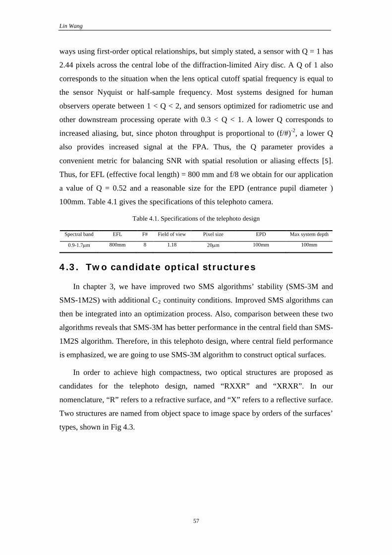
Lin Wang
57
ways using first-order optical relationships, but simply stated, a sensor with Q = 1 has
2.44 pixels across the central lobe of the diffraction-limited Airy disc. A Q of 1 also
corresponds to the situation when the lens optical cutoff spatial frequency is equal to
the sensor Nyquist or half-sample frequency. Most systems designed for human
observers operate between 1 < Q < 2, and sensors optimized for radiometric use and
other downstream processing operate with 0.3 < Q < 1. A lower Q corresponds to
increased aliasing, but, since photon throughput is proportional to (f/#)-2, a lower Q
also provides increased signal at the FPA. Thus, the Q parameter provides a
convenient metric for balancing SNR with spatial resolution or aliasing effects [5].
Thus, for EFL (effective focal length) = 800 mm and f/8 we obtain for our application
a value of Q = 0.52 and a reasonable size for the EPD (entrance pupil diameter )
100mm. Table 4.1 gives the specifications of this telephoto camera.
Table 4.1. Specifications of the telephoto design
Spectral band EFL F# Field of view Pixel size EPD Max system depth
0.9-1.7µm 800mm 8 1.18 20µm 100mm 100mm
4.3. Two candidate optical structures
In chapter 3, we have improved two SMS algorithms’ stability (SMS-3M and
SMS-1M2S) with additional C2 continuity conditions. Improved SMS algorithms can
then be integrated into an optimization process. Also, comparison between these two
algorithms reveals that SMS-3M has better performance in the central field than SMS-
1M2S algorithm. Therefore, in this telephoto design, where central field performance
is emphasized, we are going to use SMS-3M algorithm to construct optical surfaces.
In order to achieve high compactness, two optical structures are proposed as
candidates for the telephoto design, named “RXXR” and “XRXR”. In our
nomenclature, “R” refers to a refractive surface, and “X” refers to a reflective surface.
Two structures are named from object space to image space by orders of the surfaces’
types, shown in Fig 4.3.

Chapter 4 Ultra-Compact SWIR telephoto camera design
58
Fig 4.3. Sketches of 2 candidate structures.
Comparing these two structures, it can be seen that:
a. Type RXXR can be made in one solid lens with two metalized surfaces, and type
XRXR can be made in two pieces (one mirror and one lens). Therefore, type
RXXR is simpler to align than type XRXR.
b. Considering the weight of the whole system, type RXXR uses more volume of
material than type XRXR. Therefore, type RXXR seems to weight more than type
XRXR.
In both structures, there are 4 surfaces to be designed. We can prescribe the frontal
surface of two structures to be a parabola, and construct the other 3 surfaces with
improved SMS-3M algorithm. The free parameter of prescribed parabola is its central
curvature, which will also be optimized. Since the design procedures for structure
RXXR and XRXR is very similar, we are going to present in detail the RXXR design
and give only results of XRXR design.
4.3.1. RXXR type optical structures
Once the central vertices positions are fixed, central segments have to be
calculated with C2 continuity condition, described in Chapter 3. Two different unique
solutions exists (shown in Fig 4.4), which have different center curvatures. The exit
refractive surface in the Fig 4.4(a) has a concave form, while in Fig 4.4(b) has a
convex form. If the sign of the focal length is reversed, two other families (not shown
in Fig 4.4) exist in which the small mirror is concave instead of convex.
(a) Type 1: RXXR (b) Type 2: XRXR
Image plane
Rpre
R X
X
Image plane
Xpre
R
X R

Lin Wang
59
(a) (b)
Fig 4.4. RXXR designs with the same vertices positions (50, 20, 49, 43 mm from sensor plane) and identical front surface with (a) concave exit refractive surface; (b) with convex exit refractive surface
The designed object angles have been selected so that their RMS2D distribution
curves (defined as the RMS spot diameter calculated with only meridian rays within
the field) present a constant ripple over the field of view. Since the SMS method
guarantees that the RMS2D is null at the design object angles, the general form of the
function RMS2D(θ) is [13,14]:
( )2 21RMS2D( ) ( )Aθ θ θ θ θ= − (4.4)
Where θ 1 is designed off-axis object angle and A(θ ) is an arbitrary even function.
Best performing SMS designs usually have A(θ) ≈ constant [13], for which Eq. (4.4)
is just the absolute value of a and 3rd order polynomial. This is the case of the concave
exit surface design on Fig 4.4(a), whose RMS2D function is plotted on Fig 4.5(a). A
3rd order polynomial has been fitted (with A=0.208 mm/deg). However, the convex
exit surface design on Fig 4.4(b) a constant A(θ) does not fit well, but a sixth-order
approximation is needed (A(θ)=1.78156−10.5θ 2+34.5628θ 4−36.4749θ 6, θ in degrees,
A in mm), as shown on Fig 4.5(b). Comparing the maximum RMS2D values for both
graphs, the concave exit surface design has much lower value than the convex one.
Therefore the concave exit surface design has a better control over all meridian rays,
and thus in the following sections, only the concave exit surface type will be
considered.

Chapter 4 Ultra-Compact SWIR telephoto camera design
60
Fig 4.5. RMS diameter of the spot produced by only meridian rays, labeled as RMS2D, for the two designs in Fig 4.4: (a) concave exit refractive surface; (b) convex exit refractive surface. The absolute value of the 3rd order best fit polynomial sharing the zeros is also shown.
1) Phase I optimization
Each of the two RXXR solutions in Fig 4.4 has 5 free parameters: the position of the 4
vertices on the optical axis which are defined as distance from the image plane, and
the on-axis curvature of the parabola. Those parameters can therefore be optimized to
minimize a certain merit function, or alternatively some of them can be fixed to
guarantee certain geometrical constraints (edge thickness, percentage of obscuration,
center thickness, manufacturability, etc). In this optimization, vertices 1, 2, and 3 are
limited within a relative small parametric range to keep the lens compact, while vertex
4 can vary in a bigger range.
Since the design is monochromatic, we have used an artificial material with a
refractive index of 1.5. Then we optimized those 5 free parameters to find a local
minimum. The initial curvature of parabola is set to 0 (as a straight line). During each
cycle, the other 3 aspheres are calculated using the SMS-3M algorithm. The merit
function for this optimization is to minimize the largest RMS3D spot size within the
field (calculated by 3D ray-tracing over the whole pupil). We have found that for a
fixed set of vertices positions, varying central curvature of frontal parabola can
always give a strong reduction to the merit function.
As a first exercise, we fix the vertices positions at the local minimum, and
optimize only the central curvature of parabola. For the design on Fig 4.4(a), the
results of the optimization of the central curvature of the front surface are shown in
Fig 4.6. It can be seen that varying the central curvature of the first surface does not
significantly change the RMS spot size for meridian rays only (i.e. the RMS2D curves
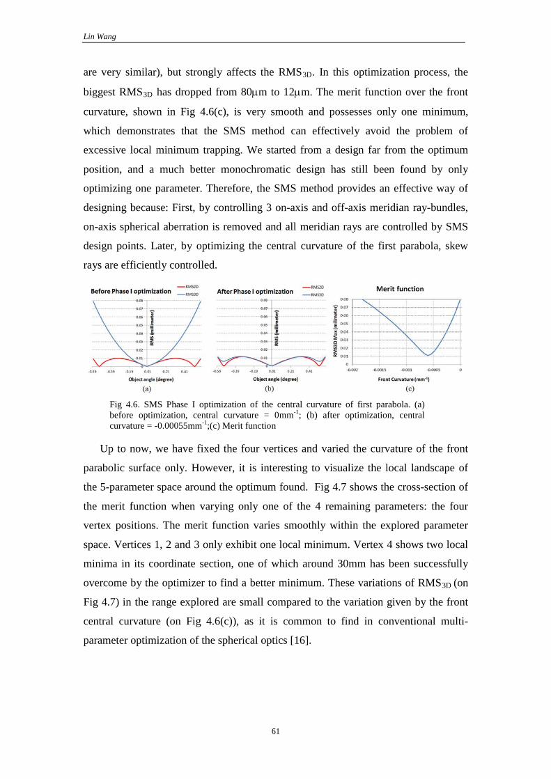
Lin Wang
61
are very similar), but strongly affects the RMS3D. In this optimization process, the
biggest RMS3D has dropped from 80µm to 12µm. The merit function over the front
curvature, shown in Fig 4.6(c), is very smooth and possesses only one minimum,
which demonstrates that the SMS method can effectively avoid the problem of
excessive local minimum trapping. We started from a design far from the optimum
position, and a much better monochromatic design has still been found by only
optimizing one parameter. Therefore, the SMS method provides an effective way of
designing because: First, by controlling 3 on-axis and off-axis meridian ray-bundles,
on-axis spherical aberration is removed and all meridian rays are controlled by SMS
design points. Later, by optimizing the central curvature of the first parabola, skew
rays are efficiently controlled.
Fig 4.6. SMS Phase I optimization of the central curvature of first parabola. (a) before optimization, central curvature = 0mm-1; (b) after optimization, central curvature = -0.00055mm-1;(c) Merit function
Up to now, we have fixed the four vertices and varied the curvature of the front
parabolic surface only. However, it is interesting to visualize the local landscape of
the 5-parameter space around the optimum found. Fig 4.7 shows the cross-section of
the merit function when varying only one of the 4 remaining parameters: the four
vertex positions. The merit function varies smoothly within the explored parameter
space. Vertices 1, 2 and 3 only exhibit one local minimum. Vertex 4 shows two local
minima in its coordinate section, one of which around 30mm has been successfully
overcome by the optimizer to find a better minimum. These variations of RMS3D (on
Fig 4.7) in the range explored are small compared to the variation given by the front
central curvature (on Fig 4.6(c)), as it is common to find in conventional multi-
parameter optimization of the spherical optics [16].

Chapter 4 Ultra-Compact SWIR telephoto camera design
62
Fig 4.7. Merit functions of vertices position optimization.
2) Phase II optimization
In Phase I the SMS surfaces are represented as NURBS splines in a C++ code. Next,
we will expand them into polynomial series and export coefficients into Code V,
where a second optimization process (Phase II) will be carried out with these
polynomials as a starting point. In this expansion, Q-con type polynomials will be
used [17], although better optimization results have been recently reported with Q-bfs
polynomials [18].
(a) Further optimization of the monochromatic design In order to verify that the Q-con polynomial representation in Code V is a good
approximation of the surfaces that we calculated with the SMS method, we compare
their RMS3D distributions, as shown in Fig 4.8(a). The two RMS3D curves are very
well matched. Three designed object angles can be seen to correspond to 3 local
minimum RMS3D values. In Fig 4.8(b), the MTF performance for all fields of view is
very close to the diffraction limit at 1,300 nm. However, further improvement for this
monochromatic design is still possible, because the RMS3D distribution curve is not
well balanced between the central field and the edge field.
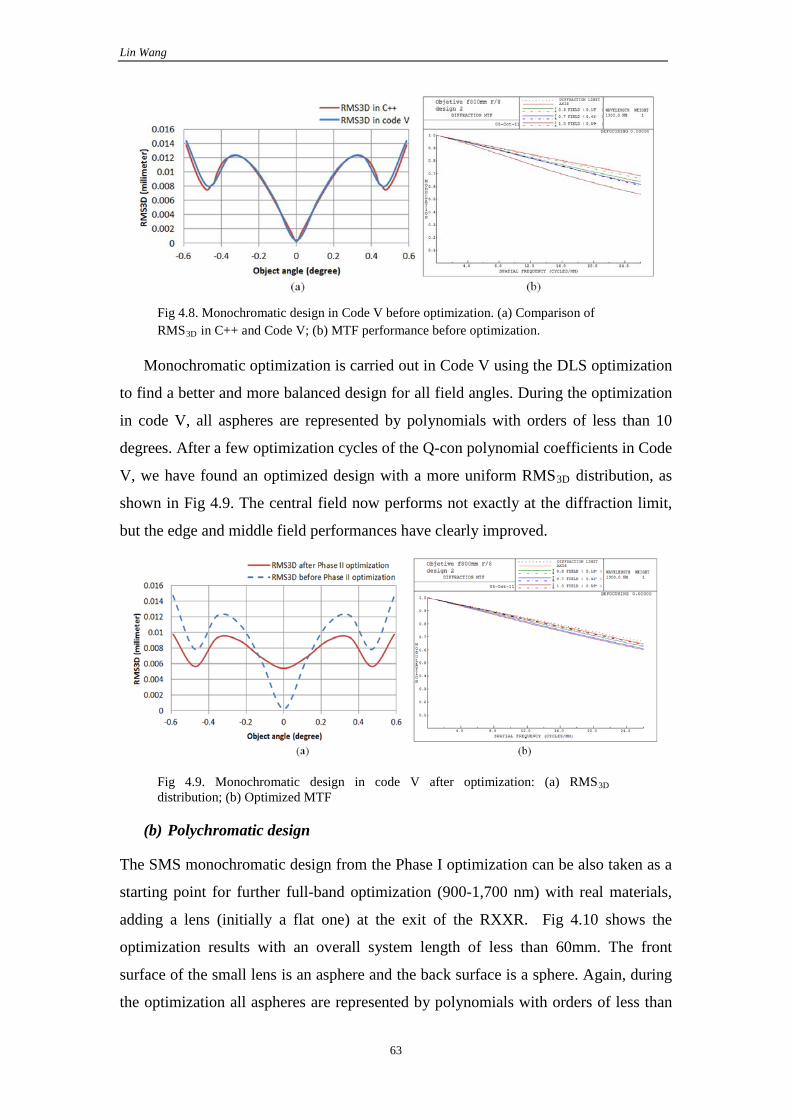
Lin Wang
63
Fig 4.8. Monochromatic design in Code V before optimization. (a) Comparison of RMS3D in C++ and Code V; (b) MTF performance before optimization.
Monochromatic optimization is carried out in Code V using the DLS optimization
to find a better and more balanced design for all field angles. During the optimization
in code V, all aspheres are represented by polynomials with orders of less than 10
degrees. After a few optimization cycles of the Q-con polynomial coefficients in Code
V, we have found an optimized design with a more uniform RMS3D distribution, as
shown in Fig 4.9. The central field now performs not exactly at the diffraction limit,
but the edge and middle field performances have clearly improved.
Fig 4.9. Monochromatic design in code V after optimization: (a) RMS3D distribution; (b) Optimized MTF
(b) Polychromatic design
The SMS monochromatic design from the Phase I optimization can be also taken as a
starting point for further full-band optimization (900-1,700 nm) with real materials,
adding a lens (initially a flat one) at the exit of the RXXR. Fig 4.10 shows the
optimization results with an overall system length of less than 60mm. The front
surface of the small lens is an asphere and the back surface is a sphere. Again, during
the optimization all aspheres are represented by polynomials with orders of less than

Chapter 4 Ultra-Compact SWIR telephoto camera design
64
10 degrees. Further reduction to the number of the aspheres’ coefficients is still
possible. The final system distortion is less than 1% and obscuration caused by central
small mirror surface is less than 5%. This simple final configuration demonstrates that
a good starting point cannot only make the design process more efficient, but also
reduces the complexity of optical systems.
Fig 4.10. RXXR achromatic design in Code V: (a) BK7 (flint) and k7 (crown) combination is used to correct chromatic aberrations; (b) MTF value is very close to the diffraction limit; (c) Ray aberrations remain small for all field angles.
Tolerance study of this RXXR design has shown that: Tolerances for tilt and
translational movement of two mirror surfaces are very tight, ±5 microns for
translational movement and 0.0050 for tilt displacements. In general, these tight
tolerances can make assembly of an optical system very impractical. However, the
RXXR type system has fewer assembly problems because two mirrors surfaces are
integrated into one solid lens. Tight tolerances can probably be dealt with during the
fabrication process. This tolerance can be relaxed reducing the system compactness.
Another design with system depth 75mm is worked out in this direction to have larger
tolerances, as shown in Fig 4.12.

Lin Wang
65
Fig 4.11. 75mm RXXR achromatic design in Code V: (a) BK7 (flint) and k7 (crown) combination is used to correct chromatic aberrations; (b) MTF value is very close to the diffraction limit; (c) Ray aberrations maintain small for all field angles.
The manufacture of a first prototype with ±10 microns with a 75 mm system
depth is now in progress. The cumulative probability prediction in Fig 4.12 indicates a
90% possibility to fabricate the prototype with MTF above 0.2.
Fig 4.12. MTF tolerance analysis in Code V of 75mm RXXR design, (F1 F2 F3 F4) in the figures corresponding to object angles (00, 0.170, 0.40, 0.580).
4.3.2. XRXR type optical structures
The procedures of XRXR type configuration is very similar to the RXXR design, here
we only present monochromatic results and polychromatic results. Fig 4.13 shows
75mm
K7
BK7
(a)
(b) (c)
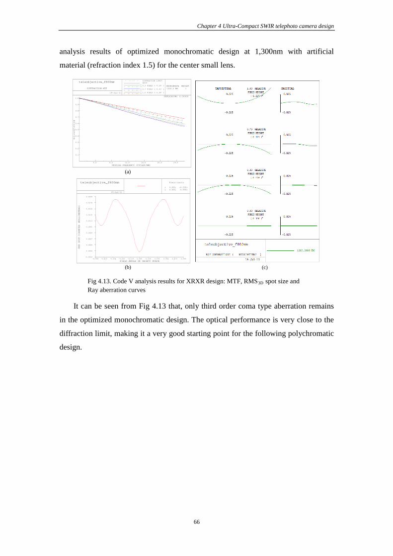
Chapter 4 Ultra-Compact SWIR telephoto camera design
66
analysis results of optimized monochromatic design at 1,300nm with artificial
material (refraction index 1.5) for the center small lens.
Fig 4.13. Code V analysis results for XRXR design: MTF, RMS3D spot size and Ray aberration curves
It can be seen from Fig 4.13 that, only third order coma type aberration remains
in the optimized monochromatic design. The optical performance is very close to the
diffraction limit, making it a very good starting point for the following polychromatic
design.
1.0
0.9
0.8
0.7
0.6
0.5
0.4
0.3
0.2
0.1
MODULATION
4.0 8.0 12.0 16.0 20.0 24.0
SPATIAL FREQUENCY (CYCLES/MM)
teleobjective_f800mm
DIFFRACTION MTF
19-Jul-11
DIFFRACTION LIMIT AXIS
T R 0.3 FIELD ( )0.18O
T R 0.7 FIELD ( )0.41O
T R 1.0 FIELD ( )0.59O
WAVELENGTH WEIGHT1300.0 NM 1
DEFOCUSING 0.00000
19-Jul-11
teleobjective_f800mm
FIELD ANGLE IN OBJECT SPACE
RMS SPOT DIAMETER (MILLIMETERS)
-0.590 -0.472 -0.354 -0.236 -0.118 0.000 0.118 0.236 0.354 0.472 0.590 -0.0018
0.0004
0.0026
0.0047
0.0069
0.0091
0.0113
0.0135
0.0156
0.0178
0.0200
Field Limits ( 0.000, -0.590) ( 0.000, 0.590)
(a)
(b) (c)

Lin Wang
67
Fig 4.14. XRXR achromatic design in Code V:MTF and Ray aberration curves, distortion< 2.5%.
In the polychromatic design, shown in Fig 4.14, an additional small lens is added
after the central small lens. The aberration curves in Fig 4.14(c) show that for all
wavelengths and field angles, chromatic aberrations have been well corrected; the
ripple shape aberration curves represent high order aberration introduced during the
optimization process, because we have employed high order (up to 20 degrees) Q-con
polynomials in the optimization. Similar to the RXXR design, alignment tolerance
(±5 microns) of the first mirror is very restricting, making the assembling of this
system almost impossible at the moment. The above XRXR type configuration
designs demonstrate once again the power of our design strategy (SMS + optimization)
in searching of good initial designs.
4.4. Conclusion
In this work, we have presented an SMS based optimization strategy, which
consists of two design phases. In the first phase, the optical system is considered as
monochromatic. The SMS method, which does not restrict the surface asphericty or
system paraxiality, is embedded in an optimization process of the free parameters
1.0
0.9
0.8
0.7
0.6
0.5
0.4
0.3
0.2
0.1
MODULATION
2.0 4.0 6.0 8.0 10.0 12.0 14.0 16.0 18.0 20.0 22.0 24.0
SPATIAL FREQUENCY (CYCLES/MM)
XRXR tele-objective f800mm
DIFFRACTION MTF
20-Jul-11
DIFFRACTION LIMIT AXIS
T R 0.3 FIELD ( )0.20O
T R 0.7 FIELD ( )0.40O
T R 1.0 FIELD ( )0.59O
WAVELENGTH WEIGHT1650.0 NM 11600.0 NM 11500.0 NM 11400.0 NM 11300.0 NM 11200.0 NM 11100.0 NM 11000.0 NM 1 900.0 NM 1
DEFOCUSING 0.00000
K7 NKF9
(a)
(b) (c)
Chapter 4 Ultra-Compact SWIR telephoto camera design
68
(vertex positions, etc), so the SMS procedure repeated in every iteration. In the second
phase, the SMS monochromatic design is used as a starting point for further
monochromatic or polychromatic optimization in Code V.
We have applied this design strategy to an ultra-compact SWIR camera design. In
order to achieve ultra-compactness, two optical architectures RXXR and XRXR are
proposed, which can fold the light in small overall system length. In the
monochromatic design, the SMS construction method is implemented with a
prescribed parabolic front surface. Two sets of central curvatures (concave type and
convex type) are then found as solutions to the C2 smoothness condition. Comparison
between these two types of solutions reveals that the concave type structure has a
better performance than the convex type.
The central curvature of the prescribed parabolic front surface is then optimized
to control skew rays. In the RXXR type configuration, by only optimizing this central
curvature, the maximum RMS spot diameter is reduced from 80µm to 12µm for the
concave type design. The landscape plot of merit function versus central vertices
demonstrates that the merit function is less sensitive to vertex positions than the
central curvature of front surface. Finally, starting from the concave type
monochromatic design, an ultra-compact well-corrected achromatic design with one
added small lens at the exit is found. Similar results have also been obtained in the
XRXR type configuration. Although from practical point of view, RXXR type design
has a better chance to be fabricated out in the near future.
References
1. GoodRich websit: http://www.sensorsinc.com/whyswir.html.
2. D. Action, et. al., “Large Format Short Wave Infrared (SWIR) Focal Plane Array (FPA) With Extremely Low Noise and High Dynamic Range,” Proc. SPIE 7298, pp. 7298-1 – 13 (2009).
3. M. MacDougal, et. al., “Low Dark Current Detector Arrays for Night Vision and Astronomy,” Proc. SPIE 7298, pp. 79823F-1 – 10 (2009).
4. J. Battaglia, et. al., “An uncooled 1280 x 1024 InGaAs focal plane array for small platform, shortwave infrared imaging,” Proc. SPIE 7298, pp. 72983C-1 – 8 (2009).
5. Terrence S. Lomheim and E.D. Hernandez-Baquero, “Translation of spectral radiance levels, band choices, and signal-to-noise requirements to focal plane specifications and design constraints,” Proc. SPIE 4486, pp. 263 (2002).
6. Craig Olson, Tim Goodman, Chris Addiego, and Steve Mifsud, “Design and construction of a short-wave infrared 3.3X continuous zoom lens” Proc. SPIE 7652, 76522A (2010).

Lin Wang
69
7. Jose M. Infante Herrero, Marta C. de la Fuente, Wang Lin, Juan Carlos Miñano Dominguez, Pablo Benítez, Guillermo Biot, Hammed Ahmadpanahi and Andres F. Cifuentes, "Design of a compact objective for SWIR applications", Proc. SPIE 8167, 81670K (2011).
8. R. Hamilton Shepard III and Scott Sparold, “Material Selection for Color Correction in the Short-wave Infrared,” Proc. SPIE 7060, pp. 70600E-1 – 10 (2008).
9. Chapter 8 in R.Winston, J.C. Miñano, P. P. Benítez, with contributions of N. Shatz, J. Bortz, "Nonimaging Optics", Academic Press Elsevier (2004).
10. Chaves, J., [Introduction to Nonimaging Optics], CRC Press, (2008).
11. Pablo Benítez, Juan C. Miñano, José Blen, Rubén Mohedano, Júlio Chaves, Oliver Dross, Maikel Hernández, and Waqidi Falicoff, “Simultaneous multiple surface optical design method in three dimensions,” Opt. Eng. 43, 1489 (2004).
12. P. Benítez and J. C. Miñano, "Ultra high-numerical-aperture imaging concentrator," J. Opt. Soc. Am. A , Vol 14 (1997).
13. J. C. Miñano, P. Benítez, Wang Lin, José Infante, Fernando Muñoz, Asunción Santamaría "An application of the SMS method for imaging designs," Optical Express, Vol 17, No. 26, p. 24036 (2009).
14. Miñano, J.C., Benítez, P., Wang Lin,, Muñoz, F., Infante, J., Santamaría, A., “Overview of the SMS design method applied to imaging optics”, Proc. SPIE 7429, 74290C (2009).
15. Jose M. Infante Herrero, Fernando Muñoz, Pablo Benitez, Juan Carlos Miñano, Wang Lin, Juan Vilaplana, Guillermo Biot, Marta de la Fuente “Novel fast catadioptric objective with wide field of view”, Proc. SPIE 7787, 778704 (2010).
16. Florian Bociort and Maarten van Turnhout, "Finding new local minima in lens design landscapes by constructing saddle points", Opt. Eng. 48, 063001 (2009).
17. G. W. Forbes, "Shape specification for axially symmetric optical surfaces," Opt. Express 15, 5218-5226 (2007).
18. G. W. Forbes, “Robust, efficient computational methods for axially symmetric optical aspheres,” Opt. Express 18(19), 19700–19712 (2010).
19. F. Muñoz, P. Benítez, and J. C. Miñano “High-order aspherics: the SMS nonimaging design method applied to imaging optics”, Proc. SPIE 7061, 70610G (2008).
20. Fernando Muñoz Doctoral Disertation “Sistemas ópticos avanzados de gran compactibiliad con aplicaciones en formación de imagen y en iluminación” UPM, Madrid (2004).
21. Orestes N. Stavroudis, “The mathematics of geometrical and physical optics”, Wiley-VCH (2006).

Chapter 5 SMS imaging design in three dimensions
70
Chapter 5. SMS imaging design in three dimensions
5.1. Introduction
Traditionally, optical designers tried to avoid the use of freeform surfaces in their
systems unless rotational optical surfaces were found incapable of achieving the
desired performance. The reasons were high fabrication cost and testing for free-form
surfaces, and the lack of efficient design tools for such surfaces. With the recent
development of diamond turned fabrication technology, optical quality mirrors
defined as a conic plus lower order terms of freeform Zernike polynomials can now
be fabricated at a more competitive cost. By breaking the symmetry that those
rotational surfaces had, free-form optical surfaces offer much more design freedoms
to optical designers, which are especially important in off-axis un-obscured mirror
systems, like long wave infrared (LWIR) reflective imagers [1] and head-mounted
displays [2]. In these off-axis systems, significant astigmatic aberrations can easily be
introduced to oblique incident rays, because mirror surfaces tend to have different
power on two principle directions if there principle curvatures are the same. These
astigmatic aberrations can be best compensated when local principle curvatures have
different values, which results in a free-from surface.
Comparing with rotational imaging optics, theories and design methods with
freeform optics have not been fully developed. Up to now, design techniques have

Lin Wang
71
emerged mainly from imaging and non-imaging fields [1-6]. Fuerschbach and
coworkers implemented a ψ−type of radial polynomials to represent and optimize
freeform surface [1]. Forbes has developed a different set of orthogonal polynomials
in the surface gradient within a given circular boundary [3]. Hick et al. employed two
freeform mirror surfaces to achieve a distortion free design [4]. Bruneton and
coworkers developed a design algorithm for a nonimaging lens with two freeform
surfaces [5]. In this work, we are going to focus on another design technique, the
SMS3D method, proposed by Benitez and Miñano [6].
The SMS method in three dimensions (SMS3D) has already been widely used in
the non-imaging optical designs to achieve maximum transfer efficiency [6-9],
particularly in chapter 6 of this thesis. The SMS3D method provides a constructive
algorithm to design two free-form optical surfaces with full control of two couples of
wave-fronts and partial control of a third couple. These properties make SMS3D
method of great interest in the free-form imaging design. One major obstacle in the
free-form imaging design is the total amount of variables used to represent free-form
surfaces. Without directly construction method, designer has to put all surfaces’
parameters into an optimizer to find local minimum. However, current optimizers
have difficulties to optimize efficiently when total amount is big. With the SMS3D
method, designer only needs to choose a convenient surface representation to the
calculated free-form surfaces and focus on other free parameters. Amount of unknown
variables are greatly reduced. Also, from imaging point of view, these two free-form
surfaces produce zero aberration for the selected object points, and low aberrations for
the around object points. By carefully placing these two nodal points within all fields,
it’s possible to reduce the average aberrations dramatically. In this chapter, we are
going to explore the imaging ability of SMS3D method with a selected example
composed of two un-obscured mirrors.
5.2. Problem description
Table 5.1. Design parameters
Object(16:9) Image(16:9) F# Magnification
13.3 X 7.5mm 6.65 X 3.725mm 2.5 0.5
In this off-axis design, two free-form mirrors will image an object plane into the
image plane. Design parameters are listed in Table 5.1. The object plane can tilt an

Chapter 5 SMS imaging design in three dimensions
72
arbitrary angle with respect to the image plane, but its normal vectors will be forced to
be contained in the x-z plane. Two free-form mirrors should not obstruct the ray paths,
as shown in Fig 5.1, and will be restricted to be also symmetric with respect to the x-z
plane with its normal vectors in that plane contained in it.
Fig 5.1. Sketch of the off-axis two-mirror design.
In order to parameterize this mirror system, we place two separate polar
systems in the object space and the image space. The image plane is fixed
horizontally with its center coincide with original point 0 of the image space
coordinate system. An original point 0’ is chosen arbitrarily in the object space. The
object plane can be moved freely in the object space; therefore 3 parameters (R0, θ0,
θn) are necessary to describe its movement, where (R0, θ0) are polar coordinates of the
center of the object plane, and θn describe the angular orientation of the object plane.
From object center to image center, we can define a chief ray, which pass intersect
Mirror 1 and Mirror 2 at point P1 (R1, θ1) and P2 (R2, θ2) respectively. The
intersection point P1 and P2 and their normal vectors acts as basal points for position
and orientation of Mirror 1 and Mirror 2. The amount of variables needed to represent
a surface can vary from 10 to 100 or even more. Let us suppose that a moderate
amount of 40 variables is necessary for each mirror. Finally, we have a total amount
of 87 unknown variables in the configuration space. Without a constructive method to
determine the initial mirrors’ shape, an optimizer probably has to start from a paraxial
D
z
x
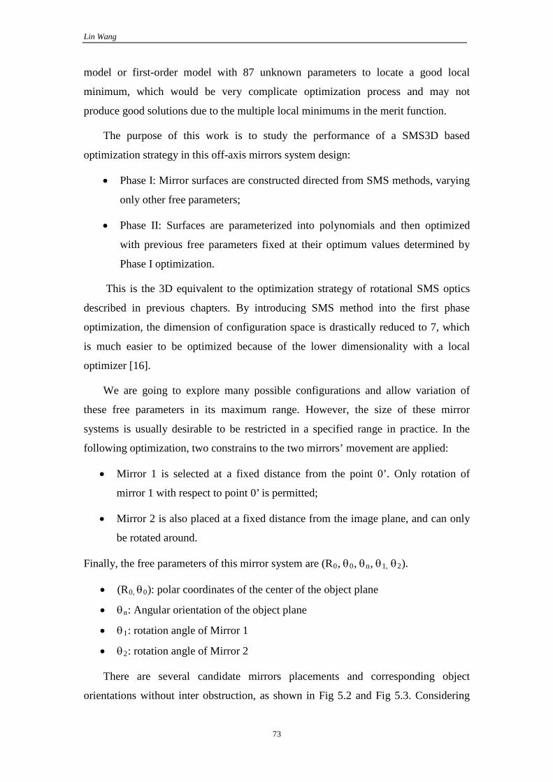
Lin Wang
73
model or first-order model with 87 unknown parameters to locate a good local
minimum, which would be very complicate optimization process and may not
produce good solutions due to the multiple local minimums in the merit function.
The purpose of this work is to study the performance of a SMS3D based
optimization strategy in this off-axis mirrors system design:
• Phase I: Mirror surfaces are constructed directed from SMS methods, varying
only other free parameters;
• Phase II: Surfaces are parameterized into polynomials and then optimized
with previous free parameters fixed at their optimum values determined by
Phase I optimization.
This is the 3D equivalent to the optimization strategy of rotational SMS optics
described in previous chapters. By introducing SMS method into the first phase
optimization, the dimension of configuration space is drastically reduced to 7, which
is much easier to be optimized because of the lower dimensionality with a local
optimizer [16].
We are going to explore many possible configurations and allow variation of
these free parameters in its maximum range. However, the size of these mirror
systems is usually desirable to be restricted in a specified range in practice. In the
following optimization, two constrains to the two mirrors’ movement are applied:
• Mirror 1 is selected at a fixed distance from the point 0’. Only rotation of
mirror 1 with respect to point 0’ is permitted;
• Mirror 2 is also placed at a fixed distance from the image plane, and can only
be rotated around.
Finally, the free parameters of this mirror system are (R0, θ0, θn, θ1, θ2).
• (R0, θ0): polar coordinates of the center of the object plane
• θn: Angular orientation of the object plane
• θ1: rotation angle of Mirror 1
• θ2: rotation angle of Mirror 2
There are several candidate mirrors placements and corresponding object
orientations without inter obstruction, as shown in Fig 5.2 and Fig 5.3. Considering

Chapter 5 SMS imaging design in three dimensions
74
that the ray path shown in Fig 5.2 is similar to number “4”, we are going to call this
type of configuration: “4” type configuration; Similarly, the configuration shown in
Fig 5.3 is called: “N” type configuration.
Fig 5.2. “4” type configuration: Object plane is relatively vertical to image plane. (a) Mirror 1 is placed above the image plane; (b) mirror 1 is placed below the image plane.
Fig 5.3. “N” type configuration: Object plane is relatively vertical to image plane. (a) Mirror 1 is placed above the image plane; (b) mirror 1 is placed below the image plane.
Since the two positions of Mirror 1 gives relatively similar information for
imaging ability of SMS3D method, we are going to discuss two orientations with
mirror 1 placed all above the image plane.
The sign of magnification between the image plane and object plane along the x
and y axis also gives 4 types of solutions, as shown in Fig 5.4. We are going to
explore optical surfaces with these four combinations.
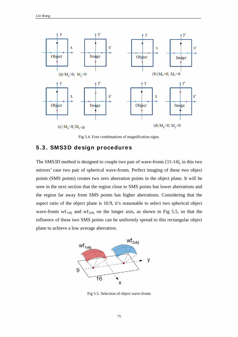
Lin Wang
75
Fig 5.4. Four combinations of magnification signs.
5.3. SMS3D design procedures
The SMS3D method is designed to couple two pair of wave-fronts [11-14], in this two
mirrors’ case two pair of spherical wave-fronts. Perfect imaging of these two object
points (SMS points) creates two zero aberration points in the object plane. It will be
seen in the next section that the region close to SMS points has lower aberrations and
the region far away from SMS points has higher aberrations. Considering that the
aspect ratio of the object plane is 16:9, it’s reasonable to select two spherical object
wave-fronts wf1obj and wf2obj on the longer axis, as shown in Fig 5.5, so that the
influence of these two SMS points can be uniformly spread to this rectangular object
plane to achieve a low average aberration.
Fig 5.5. Selection of object wave-fronts
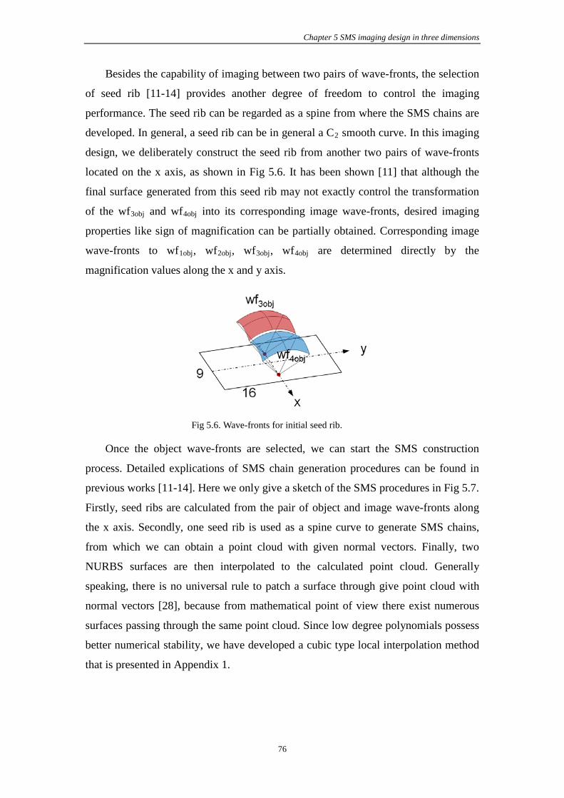
Chapter 5 SMS imaging design in three dimensions
76
Besides the capability of imaging between two pairs of wave-fronts, the selection
of seed rib [11-14] provides another degree of freedom to control the imaging
performance. The seed rib can be regarded as a spine from where the SMS chains are
developed. In general, a seed rib can be in general a C2 smooth curve. In this imaging
design, we deliberately construct the seed rib from another two pairs of wave-fronts
located on the x axis, as shown in Fig 5.6. It has been shown [11] that although the
final surface generated from this seed rib may not exactly control the transformation
of the wf3obj and wf4obj into its corresponding image wave-fronts, desired imaging
properties like sign of magnification can be partially obtained. Corresponding image
wave-fronts to wf1obj, wf2obj, wf3obj, wf4obj are determined directly by the
magnification values along the x and y axis.
Fig 5.6. Wave-fronts for initial seed rib.
Once the object wave-fronts are selected, we can start the SMS construction
process. Detailed explications of SMS chain generation procedures can be found in
previous works [11-14]. Here we only give a sketch of the SMS procedures in Fig 5.7.
Firstly, seed ribs are calculated from the pair of object and image wave-fronts along
the x axis. Secondly, one seed rib is used as a spine curve to generate SMS chains,
from which we can obtain a point cloud with given normal vectors. Finally, two
NURBS surfaces are then interpolated to the calculated point cloud. Generally
speaking, there is no universal rule to patch a surface through give point cloud with
normal vectors [28], because from mathematical point of view there exist numerous
surfaces passing through the same point cloud. Since low degree polynomials possess
better numerical stability, we have developed a cubic type local interpolation method
that is presented in Appendix 1.

Lin Wang
77
Fig 5.7. SMS design procedures. (a) selection of two pairs of wave-fronts on x axis; (b) construction of seed rib from x axis wave-fronts; (c) selection of two pairs of wave-fronts on y axis; (d) SMS chains from seed rib with y axis wave-fronts.
5.4. Phase I: Free parameters optimization
In this sections, optical configurations shown in Fig 5.2(a) and Fig 5.3(a) are going to
be explored, each of which are designed with 4 types of magnification combinations
explained in Fig 5.4. The merit function for evaluation is given as:
2 21 2
1( )
Fields
i i i ii
Merit Function W Rms W Distortion=
= +∑ (5.1)
where W1i and W2i are arbitrarily selected weights in order to balance the RMS and
distortion performance.
5.4.1. “4” type configurations
Two freeform mirrors are generated constantly with SMS3D method in each
optimization cycle with different free-parameters. For the SMS design, we have
selected the image wave-fronts centered at (±2mm, 0). The object wave-fronts are
decided by the magnification values.
Fig 5.8 shows an optimized design with magnification 0.5 and type “Mx+My+”.
From Fig 5.8(a) and Fig 5.8(b), it can be seen that there is no internal caustics
between two freeform mirrors due to the selection of signs of magnification. There are
(a)
(b)
(c)
(d)
Seed rib SMS chains
x
y z

Chapter 5 SMS imaging design in three dimensions
78
two lowest RMS value appeared in Fig 5.8(c), which correspond to the design image
points. Region close to the two design image points has lower RMS values, and
region far away has higher RMS values. Average RMS value on the image plane is
6µm, and the maximum distortion in Fig 5.8(d) is less than 0.3%.
Fig 5.8. Optimized design of magnification type “Mx+ My+”. (a) Front view (b) Perspective view (c) RMS max = 15µm, RMS min = 1µm, RMS average = 6µm (d) Distortion < 0.3%.
Fig 5.9 shows an optimized design with magnification 0.5 and type “Mx+My-”.
From Fig 5.9(a), it can be seen that there is no internal caustics in the “XZ” plane,
while caustics appears in the “Y” direction due to the negative sign of “My”
magnification. Average RMS value on the image plane is 29.1µm, and the maximum
distortion is less than 1.2%.

Lin Wang
79
Fig 5.9. Optimized design of magnification type “Mx+ My-”. (a) Front view (b) Perspective view (c) RMS max = 57µm, RMS min = 5.7µm, RMS average = 29.1µm (d) Distortion < 1.2%.
Fig 5.10 shows an optimized design with magnification 0.5 and type “Mx-My+”.
From Fig 5.10(a), it can be seen that caustics is in the “XZ” plane due to the negative
sign of “Mx”, while no caustics appears in the “Y” direction. Average RMS value on
the image plane is 27.4µm, and the maximum distortion is less than 0.3%.
Fig 5.10. Optimized design of magnification type “Mx- My+”. (a) Front view (b) Perspective view (c) RMS max = 52µm, RMS min = 4µm, RMS average = 27.4µm (d) Distortion < 0.3%

Chapter 5 SMS imaging design in three dimensions
80
Fig 5.11 shows an optimized design with magnification 0.5 and type “Mx-My-”.
From Fig 5.11
(a), it can be seen that caustics occurs in both the “XZ” plane and in the “Y”
direction. In this “--” type configuration, an optimum design is hard to find, because
when parameters are changed, the caustics moves quickly to one of these two mirrors,
making it unstable for the surface construction. Here we only present an initial design
at a non-optimum position in the parametric space.
Fig 5.11. Optimized design of magnification type “Mx- My-” (a) Front view (b) Perspective view.
5.4.2. “N” type configurations
The procedures to explore “N” type configurations is similar to the “4” type
configurations. In “N” type cases, the object plane is placed relatively horizontal. Fig
5.12 shows an optimized design with magnification 0.5 and type “Mx+My+”. From
Fig 5.12(a) and Fig 5.12(b), it can be seen that there is no internal caustics between
two mirrors. Average RMS value on the image plane is 5µm, and the maximum
distortion is less than 0.6%.

Lin Wang
81
Fig 5.12. Optimized design of magnification type “Mx+ My+”. (a) Front view (b) Perspective view (c) RMS max = 12µm, RMS min = 0.78µm, RMS average = 5µm (d) Distortion < 0.6%.
Fig 5.13 shows an optimized design with magnification 0.5 and type “Mx+My-”.
From Fig 5.13(a) and Fig 5.13(b), it can be seen that there is no internal caustics in the
“XZ” plane, while caustics appears in the “Y” direction due to the negative sign of
“My” magnification. Average RMS value on the image plane is 30µm, and the
maximum distortion is less than 0.5%.
Fig 5.13. Optimized design of magnification type “Mx+ My-”. (a) Front view (b) Perspective view (c) RMS max = 62µm, RMS min = 5.9µm, RMS average = 30µm (d) Distortion < 0.5%.
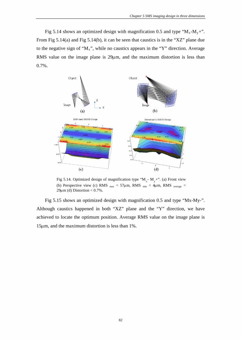
Chapter 5 SMS imaging design in three dimensions
82
Fig 5.14 shows an optimized design with magnification 0.5 and type “Mx-My+”.
From Fig 5.14(a) and Fig 5.14(b), it can be seen that caustics is in the “XZ” plane due
to the negative sign of “Mx”, while no caustics appears in the “Y” direction. Average
RMS value on the image plane is 29µm, and the maximum distortion is less than
0.7%.
Fig 5.14. Optimized design of magnification type “Mx- My+”. (a) Front view (b) Perspective view (c) RMS max = 57µm, RMS min = 4µm, RMS average = 29µm (d) Distortion < 0.7%.
Fig 5.15 shows an optimized design with magnification 0.5 and type “Mx-My-”.
Although caustics happened in both “XZ” plane and the “Y” direction, we have
achieved to locate the optimum position. Average RMS value on the image plane is
15µm, and the maximum distortion is less than 1%.

Lin Wang
83
Fig 5.15. Optimized design of magnification type “Mx- My-”. (a) Front view (b) Perspective view (c) RMS max = 36µm, RMS min = 2.6µm, RMS average = 15.6µm (d) Distortion < 0.7%.
In summary, the analysis results of the explored configurations are listed in Table
5.2. The best results are given by the “Mx+My+” type magnification in both types of
configurations. Comparing the shape of this “Mx+My+” type with other types, the
“Mx+My+” type results in a smoother and more planar shape than other types. The
“Mx-My+” and “Mx+My-” type designs have similar performance respecting the
RMSavg value.
Table 5.2. Summary of optimization results
Mx+ My+ Mx+ My- Mx- My+ Mx- My-
“4” type Configuration RMSAvg = 6µm Distortion < 0.2%
RMS Avg = 29.1 µm Distortion < 1.2%
RMSAvg = 27.4 µm Distortion < 0.3% Failed
“N” type Configuration RMSAvg = 5 µm Distortion < 0.6%
RMSAvg = 30 µm Distortion < 0.5%
RMSAvg = 30 µm Distortion < 0.7%
RMSAvg = 15 µm Distortion < 1%
5.5. Phase II: Free form surfaces optimization
In this section, we are going to optimize the design shown in Fig 5.9 using design
freedoms of two mirrors. Previous free parameters will be now fixed at their
optimized positions of phase I optimization. Since our surfaces are represented by

Chapter 5 SMS imaging design in three dimensions
84
Nurbs in our C++ program, it’s necessary to approximate these two mirrors with other
polynomials, like Forbes polynomials from freeform surface [3]. Fig 5.16 and Fig
5.17 show the surface approximation with Forbes Qbfs type polynomials and system
set up in Code V. The approximation error is estimated as the average deviation
between surface point cloud and approximated surface.
Fig 5.16. Forbes polynomials approximation with redial orders 5 and azimuthal orders 4. (a) Mirror 1 approximation error 0.1µm (b) Mirror 2 approximation error 0.05µm.
Fig 5.17. “4” type and “Mx+ My-” magnification configuration set up in Code V.
The merit function for optimization has the same format as described in Eq.
(5.1). Fig 5.18(a) gives the RMS spot diameter distribution after 10 cycles of
optimization in Code V. Comparing to the starting design that has 29.1µm average
RMS value, this optimized design has reduced the RMS average value to 15µm. The
MTF performance shown in Fig 5.18(b) is close to diffraction limit, and distortion
grid in Fig 5.18(c) also demonstrates little distortion.
(a) Mirror 1 (b) Mirror 2
Object
Image
Mirror 2
Mirror 1

Lin Wang
85
Fig 5.18. Analysis results after Code V optimization.
Therefore, after 10 cycles of optimization within Code V, a much better design
is successfully found starting from the initial design provided by phase I optimization,
which demonstrates partially the efficiency of our proposed optimization strategy. In
the future research work, more realistic models will be tested with our optimization
strategies.
5.6. Conclusion and future work
In this work, we have explored eight types’ designs of two configurations. The
SMS3D design method combined with optimization process demonstrates to be an
effective and fast way in finding local optimum with reduced amount of parameters.
Unlike the rotational symmetrical systems, where aberration theory has been well
developed and understood, utilization of freeform surfaces in non-symmetrical
systems introduce new design freedoms, meanwhile also introduce new types of
aberrations. The next step will be the quantitative analysis for different types of
aberration in these freeform designs. The potential insight from these quantitative
analyses will help designer to understand even deeper the aberration theory in the
Two mirror imaging system
27-Sep-12
RMS SPOT DIAMETERvs
OBJECT HEIGHT
Minimum = 0.0087026Maximum = 0.025146Average = 0.015023Std Dev = 0.0041358
0.26mm
-10 -5 0 5 10
X Object Height - mm
-10
-5
0
5
10Y Object Height - mm
Two mirror imaging system 27-Sep-2012
Parax FOV
Actual FOV
HORIZONTAL FOV
VERTICAL FOV
Anamorphic Ratio (Y/X) = -0.97894
(a) RMS spot diameter
(b) MTF performance
(c) Distortion grid
1.0
0.9
0.8
0.7
0.6
0.5
0.4
0.3
0.2
0.1
MODULATION
60 120 180 240 300 360 420 480 540 600
SPATIAL FREQUENCY (CYCLES/MM)
X
Y
two mirror imaging system
DIFFRACTION MTF
27-Sep-12
DIFFRACTION LIMIT Y X (-0.89,0.000) DEG Y X (0.885,0.000) DEG Y X (0.000,-0.51) DEG Y X (0.000,0.510) DEG
WAVELENGTH WEIGHT 587.6 NM 1
DEFOCUSING 0.00000

Chapter 5 SMS imaging design in three dimensions
86
freeform design, and how to make use of the design freedoms provided by freeform
surfaces.
References
1. Kyle Fuerschbach, Jannick P. Rolland, and Kevin P. Thompson, "A new family of optical systems employing φ-polynomial surfaces," Opt. Express 19, 21919-21928 (2011)
2. D. Cheng, Y. Wang, H. Hua, and M. M. Talha, “Design of an optical see-through head-mounted display with a low f-number and large field of view using a freeform prism,” Appl. Opt. 48, 2655-2668 (2009)
3. G. W. Forbes, "Characterizing the shape of freeform optics," Opt. Express 20, 2483-2499 (2012)
4. R. Andrew Hicks and Christopher Croke, "Designing coupled free-form surfaces," J. Opt. Soc. Am. A 27, 2132-2137 (2010)
5. Adrien Bruneton, Axel Bäuerle, Peter Loosen and Rolf Wester, "Freeform lens for an efficient wall washer", Proc. SPIE 8167, 816707 (2011)
6. Juan C. Miñano, Pablo Benítez, José Blen, and Asunción Santamaría, "High-efficiency free-form condenser overcoming rotational symmetry limitations," Opt. Express 16, 20193-20205 (2008)
7. Aleksandra Cvetkovic, Oliver Dross, Julio Chaves, Pablo Benitez, Juan C. Miñano, and Rubén Mohedano, "Etendue-preserving mixing and projection optics for high-luminance LEDs, applied to automotive headlamps," Opt. Express 14, 13014-13020 (2006)
8. P. Benítez, J. C. Miñano, J. Blen, R. Mohedano, J. Chaves, O. Dross, M. Hernández, J. Alvarez, W. Falicoff. “SMS Design Method in 3D Geometry: Examples and Applications,” Proc. SPIE 5185, 18-29 (2003)
9. R. Winston, J. C. Miñano, and P. Benítez, Nonimaging Optics, (Academic Press, New York, 2005)
10. Florian Bociort and Maarten van Turnhout, "Finding new local minima in lens design landscapes by constructing saddle points", Opt. Eng. 48, 063001 (2009)
11. Pablo Benítez, Juan C. Miñano, José Blen, Rubén Mohedano, Júlio Chaves, Oliver Dross, Maikel Hernández and Waqidi Falicoff, "Simultaneous multiple surface optical design method in three dimensions", Opt. Eng. 43, 1489 (2004)
12. José Blen Flores, Doctoral Thesis “Design of multiple free-form optical surfaces in 3D” E.T.S.I.Telecomunicación, (2007)
13. A. Cvetković, Doctoral Thesis “Free-form optical systems for non-imaging applications”, E.T.S.I.Telecomunicación, (2009)
14. Oliver Dross, Ruben Mohedano, Pablo Benitez, Juan Carlos Minano, Julio Chaves, Jose Blen, Maikel Hernandez and Fernando Munoz, "Review of SMS design methods and real-world applications", Proc. SPIE 5529, 35 (2004)
15. Les Piegl, Wayne Tiller, the Nurbs Book, (Springer 2nd edition 1997)
16. Michael J.Kidger, Fundamental Optical Design, (SPIE Press Monograph Vol. PM92, 2001)

Chapter 6 Étendue-squeezing condenser optics
87
Chapter 6. Étendue-squeezing condenser optics
6.1. Statement of the problem
The organizing committee of the International Optical Design Conference 2010
proposed one illumination design problem. It consisted in transferring maximum
monochromatic flux from a 1-mm-square Lambertian source in air to an equal-
étendue non-immersed target. The target surface was rectangular with 16:9 aspect
ratios. The surface area of the target must be at least 4 mm². The target was defined
such that only rays incident on the target surface at angles of θmax or less, relative to
the surface normal, are considered to be within the phase space of the target, where
the value of θmax is determined by the equal-étendue requirement. There are also some
assumptions and constrains for this design problem:
• Mirror reflectivity = 95% at all angles.
• TIR reflectivity = 100% at all angles.
• Bulk absorption loss for all dielectric materials = 0.5% per cm.
• Fresnel losses at air-dielectric interfaces = 2% at all angles.
• Fresnel losses between two different dielectric interfaces = 0.2% at all angles.
• No Fresnel losses within a gradient index material.
• Minimum size of a component and edge thickness = 0.1 mm.
• Minimum air space between components (including source) = 0.1 mm
• No volume or surface scattering.
• Light that finds its way back into the source is fully absorbed.

Lin Wang
88
The objective of this illumination design was to achieve energy transmission
efficiency as high as possible under these given assumptions and constrains.
In this chapter, I am going to present the design that I submitted with the
contribution of my PhD advisor. Our design, shown in Fig 6.1, contains two parts: a
collimator with two grooved-mirrors, and a freeform étendue-squeezer lens array to
achieve the desired aspect ratio. In Section 6.2, design principles for collimator are
illustrated. Section 6.3 describes the design principles for free-form lens array and
Section 6.4 gives the simulation results for our final design.
Fig 6.1. Sketch of proposed design for IODC 2010 illumination problem.
6.2. Collimator design with grooved mirrors
The collimator was first designed using two mirror surfaces by the SMS method
[1,2,3] to collimate the light from light source into far field. However, as illustrated in
the previous section, each mirror surface has only 95% reflectivity, with 5% energy
loss. If the collimator is made up of two planar mirror surfaces, approximately 10%
losses will be expected, lowering significantly the total energy transmission efficiency.
It is then necessary to replace these mirror surfaces with other more energy efficient
optical surfaces, and we selected. V-grooved type surfaces [4,5]. In ref [4], an
analytical method has been developed to design free-form grooved surfaces. In ref [5],
it has been observed that when the size of grooved surface is small, the cross-section
of each groove is merely a 900 corner. In this design, we are going to consider only
small grooved surfaces, as shown in Fig 6.1.
Collimator with grooved mirror surfaces
Freeform lens array
Light source z
x
y

Chapter 6 Étendue-squeezing condenser optics
89
Since there is no restriction on the design parameters, we then selected the design
parameters for our convenience which is listed in Table 6.1. The optical axis is
assigned as “y” axis and points are expressed as (x,y,z) coordinates in millimeter.
Table 6.1. Design parameters for collimator
Size of square light source 1×1mm2
Diameter of output aperture 400mm
Central position of light source (0,0,0)mm
Central position of top mirror (0,0,20)mm
Central position of bottom mirror (0,0,-100)mm
Focal length 200mm
Fig 6.2. Étendue at input and exit aperture.
Considering the hemispherical emission from each point on the rectangular light
source, shown in Fig 6.2-Left, the input étendue of the light source can be calculated
in spherical coordinates as:
02 90
2
0 0
sin cos ( )input sourceEtendue A d d mmπ
θ θ θ ψ π= =∫ ∫ (6.1)
Where θ is the altitude angle with respect to z axis and ψ is the azimuth angle.
Since this collimator is designed to have a focal length 200mm, far field image
shown in Fig 6.2-right can be estimated as a square of 0.28640×0.28640. Then étendue
at the exit aperture is:
22 0
20.2864in cos ( )4 180input exit
Square
DEtendue A s d d mmπ πθ θ θ ψ
= =
∫∫ (6.2)
Where D is the diameter of exit aperture to be determined.

Lin Wang
90
The conservation of étendue at the input and exit aperture will give the diameter
of the exit aperture “D” to be 400mm.
6.2.1. Collimator design with SMS-2D method
Jeffery has already developed for solar concentration an analytical technique to
find aplanatic optics [6]. However, since the SMS-2D method has been proved to be
an extension to classical which is more suitable to deal with extended light source [7],
therefore in this work, we will employ the SMS method in our collimator design.
Mirrors’ profile is going to be calculated in the meridian plane as curves and then
rotated around the optical axis (“y” axis) to obtain surfaces. The first step is wave-
front selections: two source wave-fronts and two far field exit wave-front. In Fig 6.3,
two spherical wave-fronts Wf1 and Wf2 are selected at the edge of light source
(±0.5mm, 0), and after transmission through will be transformed into two planar
wave-fronts Wf1’ and Wf2’ respectively.
Fig 6.3. Selection of Wave-fronts on the source and at the exit.
The exit angle of wave-front Wf1’ and Wf2’ can be calculated using focal length
given in Table 6.1, which are ±0.14320. Then the SMS chains [3,2] are built
sequentially with optical path lengths between corresponding source and exit wave-
fronts. Fig 6.4 plots the mirrors’ 2D cross-section and 3D rotational model.

Chapter 6 Étendue-squeezing condenser optics
91
Fig 6.4. 2D model and 3D model of SMS mirror design
In order to count in the obscuration of the source inside this collimator system,
the surfaces of light source are set to be absorptive; while mirror surfaces are have
only 95% reflectivity. Fig 6.5 gives the far field intensity distribution with 89.321% of
power transmission efficiency. Types of losses include:
• First obscuration of light source to the first mirror;
• Second obscuration of first mirror to the second mirror;
• Absorption on two mirrors.
However, the first obscuration is also contained in the second obscuration, due to
the big size of the first mirror, so in the following analysis, only second obscuration
and absorption will be considered. Theoretical estimation of different loss
contributions are listed in Table 6.2 and Table 6.3. In these two tables, it’s obviously
that the mirrors’ absorption counts for the major losses. This well proportionated
square far field intensity pattern shown in Fig 6.5 also indicates that the collimator is a
good imaging device under this constant focal length.
Caustics
Light source
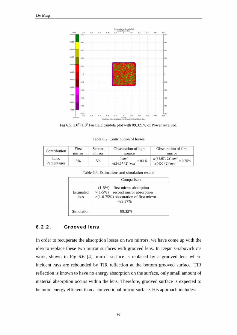
Lin Wang
92
Fig 6.5. 1.00×1.00 Far field candela plot with 89.321% of Power received.
Table 6.2. Contribution of losses
Contribution First mirror
Second mirror
Obscuration of light source
Obscuration of first mirror
Loss Percentages 5% 5%
2
2 2
1 0.1%(34.67 / 2)
mmmmπ
= 2 2
2 2
(34.67 / 2) 0.75%(400 / 2)
mmmm
ππ
=
Table 6.3. Estimations and simulation results
Comparison
Estimated loss
(1-5%) first mirror absorption ×(1-5%) second mirror absorption ×(1-0.75%) obscuration of first mirror =89.57%
Simulation 89.32%
6.2.2. Grooved lens
In order to recuperate the absorption losses on two mirrors, we have come up with the
idea to replace these two mirror surfaces with grooved lens. In Dejan Grabovickic’s
work, shown in Fig 6.6 [4], mirror surface is replaced by a grooved lens where
incident rays are rebounded by TIR reflection at the bottom grooved surface. TIR
reflection is known to have no energy absorption on the surface, only small amount of
material absorption occurs within the lens. Therefore, grooved surface is expected to
be more energy efficient than a conventional mirror surface. His approach includes:

Chapter 6 Étendue-squeezing condenser optics
93
Fig 6.6. Design principles of grooved mirror surface [4]
1. Calculate guiding lines of grooved surfaces.
2. Solve differential equations to obtain border portion of two free-form wall
surfaces.
3. Construct each groove with the SMS method to coupe WFA into WFB, which
are input and out wave-fronts.
There is one useful conclusion from his work that two freeform walls forming
each groove should intersect each other at right angle. When small grooves are
considered, linear cross-section is a good approximation to these two free-form walls
like a retro-reflector. Although the reflection can be realized by double TIR reflection
on retro-reflector, there is a still difference between conventional mirror and a retro-
reflector. Fig 6.7 shows a comparison between a planar mirror and one groove: If a
ray with cosine direction (p, q, r), impinge on a conventional mirror whose normal
vector is the Z axis, the cosine direction of reflected ray should be (p, q, -r). However,
a retro-reflector not only reverses the r component but also q component, so that the
reflected ray from a retro-reflector has a cosine direction (p, -q, -r).
Fig 6.7. Ray reflection on a retro-reflector
y
x z

Lin Wang
94
To replace a rotational mirror, the guide lines are contained in axial planes, and each
small groove extends at right angle from the guide line [5]. The skewness of a
rotational system in a meridian plane (X-Z) is calculated as:
ˆ( ,0,0) ( , ,0) ( )S x p q xq z= × =
(6.3)
The skewness of a rotational system with mirror surfaces is conserved; while for a
grooved surface, which is not rotational, the skewness is reversed due to the double
TIR reflection at two side walls of a groove. Ref [5] uses this property to mix multi-
color LEDs. Fig 6.8 is one model with two mirror surfaces replaced by two grooved
lens. The number of grooves on each grooved lens can be selected freely. The larger
number, the smaller each groove.
Fig 6.8. Collimator with two grooved lenses
In order to make clear the effects of skewness reversion, we have simulated
several models with and without grooved surfaces for the limit case of an infinite
number of infinitesimal grooves, as shown in Fig 6.9. Two conventional mirrors in
Fig 6.9(a) produces a good far filed image as expected; when one conventional mirror
is replaced by a groove lens in Fig 6.9(b), the skewness reversion causes far field to
be rotational, losing the imaging properties; when both mirrors are replaced by
grooved lens in Fig 6.9(c), the two skewness reversions after two grooved lens finally
cancel the reversion effect, so that far field rectangular image is restored. This device
is, as far as we know, the first imaging device with grooved reflectors.

Chapter 6 Étendue-squeezing condenser optics
95
Fig 6.9. Comparison of far field intensity distribution with and without grooved surfaces
Then, we have simulated a more realistic model with 9000 grooves on each
grooved lens. In the 0.80×0.80 observing window, a 98.9% collecting efficiency is
achieved, with only small material absorption and small amount of stray rays. The
intensity distribution is shown in Fig 6.10. It’s clear that using grooved lens can
significantly restore the lost by two mirrors’ absorption.
Fig 6.10. Far field intensity distribution for two 9000-grooves lenses
6.3. Étendue-squeezing lens array
An étendue-squeezer can be considered as an afocal imaging device, but with
different angular magnification value along horizontal and vertical. In ref [8], Blen
has developed design techniques necessary for an étendue-squeezer. An étendue-
squeezer can efficiently modify the shape of an output beam, and may have
applications in automotive lighting and video projectors. Because the illumination
(a) Two metalized mirrors (b) One metalized mirror and one grooved surface
(c) Two grooved lenses
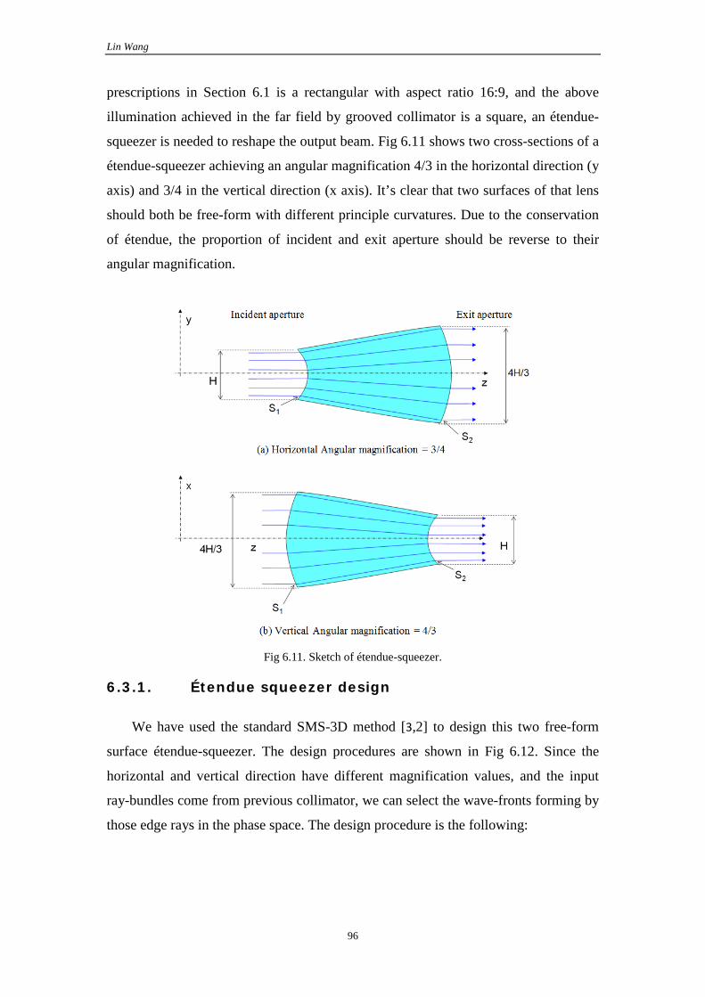
Lin Wang
96
prescriptions in Section 6.1 is a rectangular with aspect ratio 16:9, and the above
illumination achieved in the far field by grooved collimator is a square, an étendue-
squeezer is needed to reshape the output beam. Fig 6.11 shows two cross-sections of a
étendue-squeezer achieving an angular magnification 4/3 in the horizontal direction (y
axis) and 3/4 in the vertical direction (x axis). It’s clear that two surfaces of that lens
should both be free-form with different principle curvatures. Due to the conservation
of étendue, the proportion of incident and exit aperture should be reverse to their
angular magnification.
Fig 6.11. Sketch of étendue-squeezer.
6.3.1. Étendue squeezer design
We have used the standard SMS-3D method [3,2] to design this two free-form
surface étendue-squeezer. The design procedures are shown in Fig 6.12. Since the
horizontal and vertical direction have different magnification values, and the input
ray-bundles come from previous collimator, we can select the wave-fronts forming by
those edge rays in the phase space. The design procedure is the following:
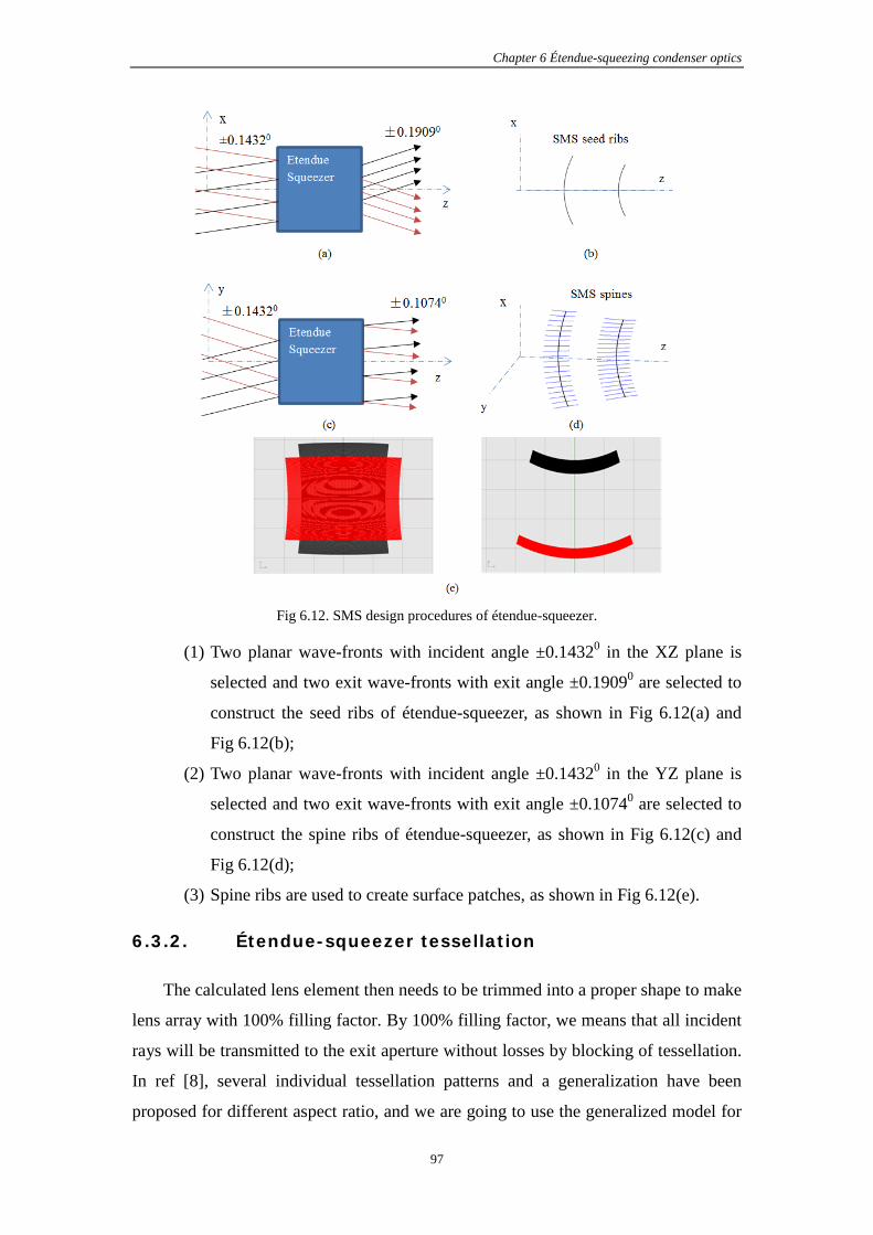
Chapter 6 Étendue-squeezing condenser optics
97
Fig 6.12. SMS design procedures of étendue-squeezer.
(1) Two planar wave-fronts with incident angle ±0.14320 in the XZ plane is
selected and two exit wave-fronts with exit angle ±0.19090 are selected to
construct the seed ribs of étendue-squeezer, as shown in Fig 6.12(a) and
Fig 6.12(b);
(2) Two planar wave-fronts with incident angle ±0.14320 in the YZ plane is
selected and two exit wave-fronts with exit angle ±0.10740 are selected to
construct the spine ribs of étendue-squeezer, as shown in Fig 6.12(c) and
Fig 6.12(d);
(3) Spine ribs are used to create surface patches, as shown in Fig 6.12(e).
6.3.2. Étendue-squeezer tessellation
The calculated lens element then needs to be trimmed into a proper shape to make
lens array with 100% filling factor. By 100% filling factor, we means that all incident
rays will be transmitted to the exit aperture without losses by blocking of tessellation.
In ref [8], several individual tessellation patterns and a generalization have been
proposed for different aspect ratio, and we are going to use the generalized model for

Lin Wang
98
our squeeze-factor 4:3, as shown in Fig 6.13. Si1 is an input surface of a lenslet and
So1 is its corresponding exit surface, whose boundaries are trimmed proportionally.
Fig 6.13. Tessellation of lens element
It’s clearer in Fig 6.14 how lenslets are placed into an array. Input and exit
surfaces’ pair is assigned the same color. The shape of each freeform surface is
“saddle-like”, because for each lenslet it’s angular diverging in one direction while
converging in the other direction.
Fig 6.14. Sketch of lenslet arrays: (a) input surface array (b) output surface array (c) Freeform “saddle” like surface.
4 3
4 3
(a) (b)
(c)
2.4cm

Chapter 6 Étendue-squeezing condenser optics
99
Since etendue squeezer should not change the size of exit aperture based on the
conservation of etendue, we need to restrict emitting area of étendue-squeeze to be
circular by putting a planar absorber at the exit with a central 200mm radial hole, as
shown in Fig 6.15. It’s interesting to observe saw-teeth near field irradiance pattern
on a dummy plane very close to the exit surface of etendue-squeezer, when the
incoming ray-bundles are circular from previous collimator. The appearance of this
saw-teeth contour is due to the limited number of array units inside the circular exit
aperture. This mismatch between exit circular aperture and saw-teeth near field
irradiance pattern will also contribute to a certain efficiency loss, which we call it
“saw-teeth loss”. Increasing the number of lenslet units can reduce the size of saw-
teeth. It can also be observed a central black area which corresponds to the blocking
by the first grooved lens of collimator. In the following analysis, 1324 units of lenslet
are placed within the exit aperture, reducing the “saw-teeth” loss to approximately
1%. Each lenslet has a 2.4 centimeters central thickness.
Fig 6.15. Circular output aperture and near field irradiance pattern.
Table 6.4 gives estimated losses that contributed by etendue-squeezer.
Table 6.4. Estimations of losses
Comparison
1324 units within exit
aperture and 2.4cm material
thickness
(1-0.5%)^2.4 material absorption ×(1-2%) Fresnel loss at first air-material interface ×(1-2%) Fresnel loss at second air-material interface ×(1-1%) Saw-teeth loss = 93.94%
400mm

Lin Wang
100
6.4. Complete system analysis
In this section, complete system analysis is conducted using both mirror
collimator and grooved lenses with free-form étendue-squeezer lenslet array to
compare their transmission efficiency. In order to reduce the size of saw-teeth, and
increase the transmission efficiency, 1342 lenslet within 400mm diameter exit
aperture have been employed. Each lenslet has a 2.4 centimeters central thickness
which will contribute to material absorption. The objective is to measure the
collection efficiency within a far field collection window within an equal-étendue
window 0.38180×0.21480.
• Metalized mirrors and étendue-squeezer
In Fig 6.16, simulation results are obtained using 100,000 rays and in total
100,000W emitting from the light source. The losses include mirrors’ absorption,
material absorption and stray ray loss. Fresnel loss however is not included but will be
counted afterwards. In the far field window 1.00×1.00 as shown in Fig 6.16(a), a good
proportionate rectangular with aspect ratio 16:9 has been observed, which
demonstrates that designed etendue-squeezer has worked properly to realize different
magnification values. The collection efficiency is 87.426%. If we further restrict the
observation within the equal etendue window 0.38180×0.21480, the collection
efficiency drops to 84.48% due to the blurred boundary, or the delusion of image
which usually happens to an extended light source. The delusion factor is then
calculated as: 84.48% 96.63%87.426%
= . Counting the Fresnel loss at two air-material
interfaces will give final transmission efficiency as 80.48%. Table 6.5 gives the
estimated transmission efficiency and simulation results. The 0.7% discrepancy is
properly due to number of rays traced and some unexpected stray rays inside the
model.

Chapter 6 Étendue-squeezing condenser optics
101
Fig 6.16. Far field collection with metalized mirrors and free-form lenslet array.
Table 6.5. Comparison of estimation and simulation results
SMS-2D XX Collimator
SMS-3D Etendue squeezing microlens array
Estimated efficiency Simulation
Diameter 400 mm metallic surfaces
1342 unit, 2.4cm thick
89.48% Collimator efficiency × 93.94% etendue-squeezer efficiency × 96.63 dilution factor = 81.2%
80.48%
16
9
(a) 10×10 far field observation window
(b) 0.38180×0.2150 far field observation window

Lin Wang
102
• Grooved lenses and étendue-squeezer
Fig 6.17 shows simulation results within 1.00×1.00 and 0.38180×0.21480
observation windows, where 200,000 rays have been traced with 200,000W power.
We can calculate from simulation results that collection efficiency is 96.15% and
90.75% respectively, which corresponds to a dilution factor: 90.75% 94.38%96.15%
= .
Discounting the two Fresnel losses results in a final transmission efficiency as
90.75%-4% = 86.75%
Fig 6.17. Simulation results with grooved collimator and free-form lenslet array.
Table 6.6 compares the estimation with simulation results for this grooved lenses
collimator and free-form lenslet array model, which has a 1.3% discrepancy. The high
16
9
(a) 10×10 far field observation window
(b) 0.38180×0.215
0 far field observation window

Chapter 6 Étendue-squeezing condenser optics
103
complexity of this model requires more rays to be traced to improve data precision.
However we didn't proceed to trace more rays because of this small discrepancy and
time-consuming ray-tracing process (almost 1 week already for these 200,000 rays).
Table 6.6. Comparison of estimation and simulation results
Grooved Collimator
SMS-3D Etendue squeezing microlens
array
Estimated efficiency Simulation
Diameter 400 mm, 9000 grooves each lens
1342 unit, 2.4cm thick
98.9% Collimator efficiency × 93.94% etendue-squeezer efficiency × 94.83 dilution factor = 88.1%
86.75%
6.5. Conclusion
This chapter has been devoted to the proposed illumination problem at 2010
IODC conference. We have come up with a novel collimator plus etendue-squeezer
optical structure to achieve high transmission efficiency. Original collimator with two
mirrors is designed by SMS-2D method and etendue-squeezer by SMS-3D method.
Since metalized mirror surfaces have almost 10% absorption loss, we have decided to
replace mirror surfaces with grooved lenses. Complete system simulation results
coincide well with estimation with only small discrepancy. We have reached
transmission efficiency as high as 86.75%.
Reference
1. R.Winston, J.C. Miñano, P. P. Benítez, with contributions of N. Shatz, J. Bortz, Nonimaging Optics, (Academic Press Elsevier, 2004), Chap. 8.
2. Chaves, J., Introduction to Nonimaging Optics, (CRC Press, 2008).
3. Pablo Benítez, Juan C. Miñano, José Blen, Rubén Mohedano, Júlio Chaves, Oliver Dross, Maikel Hernández, and Waqidi Falicoff, “Simultaneous multiple surface optical design method in three dimensions,” Opt. Eng. 43, 1489 (2004).
4. Dejan Grabovičkić, Pablo Benítez, and Juan C. Miñano, "Free-form V-groove reflector design with the SMS method in three dimensions," Opt. Express 19, A747-A756 (2011).
5. Dejan Grabovičkić, Pablo Benítez, and Juan C. Miñano, "TIR RXI collimator," Opt. Express 20, A51-A61 (2012).
6. Jeffrey M. Gordon, "Aplanatic optics for solar concentration," Opt. Express 18, A41-A52 (2010).
7. Juan C. Miñano, Pablo Benítez, Wang Lin, José Infante, Fernando Muñoz, and Asunción Santamaría, "An application of the SMS method for imaging designs," Opt. Express 17, 24036-24044 (2009).
8. José Blen Flores, Doctoral Thesis “Design of multiple free-form optical surfaces in 3D” 2007.

Chapter 7 Single freeform reflector design for concentration photovoltaic
104
Chapter 7. Single Free-Form reflector design for concentration photovoltaic
7.1. Introduction
Parabolic type mirrors have long been used as solar concentrators for high
concentration. This type of parabolic mirror designs produce a highly non-uniform
illumination, as it is known, non-uniform irradiance on the solar cell drops the
efficiency and reliability of solar cell significantly. The objective of this research is to
achieve uniform irradiance with average value around 1,500 suns at 650X
concentration ratio.
One important optical concept in solar concentrator is the acceptance angle [1-6],
which defines the angular range of incident rays that can reach the solar cell. In real
measurement, the acceptance angle is taken when the transmission efficiency has
dropped to 90%, as shown in Fig 7.1[3]. That’s to say, the minimum acceptance angle
of a solar concentrator should be greater than 0.2650 in order to collect all the sunlight
at normal incidence position. Acceptance angle of a solar concentrator is an
important factor to indicate system’s feasibility, considering those imperfections of
tracking system: tracking inaccuracy, imperfectly assembled components, imperfectly
manufactured optics, movement of system due to wind, etc. In this sense, a tracking
system with an acceptance angle 0.2650 is impractical, because it requires all system
components to operate at perfect condition. Usually, a bigger acceptance angle of the
solar concentrator can effectively relax the tolerance requirements for other system
components.

Lin Wang
105
Fig 7.1. Definition of acceptance angle.
Another useful merit function for CPV optics is the concentration-acceptance
product [4,6], which is defined as:
singCAP C α= (7.1)
Where Cg is the geometric concentration, defined as the ratio of concentrator area to
solar cell area, α is the acceptance angle. It is remarkable that for a given concentrator
architecture, the CAP is rather constant with Cg. This means that if we know the
acceptance angle at a given concentration, Eq. (7.1) can be used to estimate the
acceptance angle that we would obtain if we designed that concentrator architecture
for a different concentration.
Fig 7.2 shows the reflection of sunlight from a parabolic mirror. At every point
on the parabolic mirror, the reflected sunlight also forms a small cone with the same
angle towards the solar cell. The solar concentrator has to follow the sun movement
during day by mounting on a solar tracker, and the whole system cost depends heavily
on the tolerances allowed by the acceptance angle of the optics.

Chapter 7 Single freeform reflector design for concentration photovoltaic
106
Fig 7.2. Sketch of parabolic mirror reflects rays from sun to solar cell
In this chapter, we will deal with the interesting problem of designing a quasi-
parabolic freeform reflector achieving high concentration, sufficient acceptance angle
and producing relative low peak irradiance on the solar cell. We will first introduce an
analytical model to the irradiance distribution of parabolic-type mirror concentrator,
and visualize in that model the reason why parabolic mirror gives a bad irradiance
distribution (hot spots in the center of the solar cell). Then starting from this analytical
model, we are going to define a min-max variation problem with several conditions,
whose optimum corresponds to a uniform irradiance distribution on solar cell. At the
end, several free-form reflectors are presented with significant improved irradiance
distribution.
7.2. Analytical model for parabolic concentrator
7.2.1. Calculations with small solar cell approximation
The size of a parabolic-type concentrator can be determined immediately, given the
size of solar cell “L” and desired acceptance angle “α”. We are going to define first
an acceptance angle circle, whose diameter “D” is given as:
2LDα
= (7.2)
Solar cell
Parabolic reflector
f
ρ
0.2650

Lin Wang
107
In Fig 7.3, any point of an acceptance angle circle substends the same acceptance
angle (±α) to an on-axis solar cell. Supposing that all possible parabolic mirrors have
the focus at the center of solar cell, it is a necessary condition that the parabolic
mirrors lay inside the acceptance angle circle, in order to guarantee 100%
transmission efficiency. At each point of the reflector, we can visualize the “pin-hole
images” images of sun and incident acceptance angle cone on the solar cell surface as
those projected through an imaginary pin-hole aperture stop located at that point. This
pin-hole image is modelled in Fig 7.3 and Fig 7.4. Since the solar cell plane intersects
the reflected cones obliquely, their images on solar cell are elliptical, and their centers
coincide with the center of solar cell. The major and minor semi-axes, “a” and “b”, of
elliptical images can be easily calculated with small solar cell assumption. As is
already known that a parabolic mirror can transform an planar wave-front to a
spherical wave-front, whose center coincide with the center of solar cell, the location
of each small sun image is determined by the central ray that in this parabolic mirror
case goes to the center of solar cell.
Fig 7.3. Parabolic mirror design with a given acceptance angle.
If the focal length of a parabolic mirror “f” is already known, point on this
parabolic mirror can be expressed with the aid of distance from point to the center of
solar cell “d” and angle “β”, whose relationship is:
21 cos
fdβ
=+
(7.3)

Chapter 7 Single freeform reflector design for concentration photovoltaic
108
Fig 7.4. calculation of “a” and “b” parameters of elliptical image.
“a” and “b” are then expressed as:
tan 2 tancos (1 cos )cos
2 tantan1 cos
sin 2 tan2
d fa
fb d
d f
α αβ β β
ααββρ β
= = + = = +
= =
(7.4)
Replacing α by αsun in Eq. (7.4), can lead to minor and mayor semi-axes of sun image,
“asun” and “bsun”. “a” and “b” can be also be expressed as a function of ρ. Just
extracting β from the third equation in Eq. (7.4) Since the size of parabolic mirror is
limited by an acceptance angle circle, given the focal length, the maximum “β” or
βmax can be deduced as:
maxmax
2cos(1 cos )
d fD D
ββ
= =+
(7.5)
Where D is the diameter of acceptance angle circle. Solving Eq. (7.5):
max
81 1cos
2
fDβ
− + += (7.6)
As an example, “a” and “b” values of elliptical images on a 1×1mm2 solar cell
formed by a 650X parabolic-type mirror, and acceptance angle 10 is given in Fig 7.5.
The parabolic mirror in this example has a circular aperture. Then diameter of
acceptance angle circle is 28.65mm, focal length of the parabolic reflector is
14.334mm, and βmax is 51.860.

Lin Wang
109
Fig 7.5. “a” and “b” parameters of elliptical images on solar cell formed by a parabolic concentrator with Cg 650X, solar cell 1×1mm2 and acceptance angle 10.
However, comparing to a circular aperture parabolic concentrator, a square
aperture is more suitable for making array concentrators, as the one shown in Fig 7.6-
Left.
Fig 7.6. Square aperture parabolic concentrator with Cg 650X, solar cell 1×1mm and acceptance angle 10.
In the square aperture case, the size of parabolic mirror is 25.5×25.5mm2 and its
diameter is 36mm. The focal length corresponding to the diagonal direction should
make sure that diagonal image on solar cell is tangent to cell’s boundary, as shown in
Fig 7.6-Right. Simple calculations with Eq. (7.4) demonstrate that when diagonal
image reaches its maximum size, the horizontal image is still within the solar cell.
Therefore, the focal length for square aperture reflector is limited by its diagonal
direction.
7.2.2. Formation of hot spot
Considering the rotational symmetry of a parabolic mirror, images of sun and cone of
acceptance angle reflected from every point of parabolic mirror are mixed rotationally
f = 14.334mm
ρmax = 14.384mm
βmax = 51.860
ρ (mm) 0 2 4 6 8 10 12 14
0
0.1
0.2
0.3
0.4
0.5
a
b

Chapter 7 Single freeform reflector design for concentration photovoltaic
110
at the center of cell, as shown in Fig 7.7, which explain the reason why there is a hot
spot on the center. For a typical parabolic design with geometric concentration high as
650, the peak irradiance can exceed 104 kW/m2, which is much bigger than the
maximum irradiance requirement of a standard solar cell. This value is lowered in
practice due to manufacturing errors in the mirror and light scatterin on the surface,
but it is useful for reference as the design value.
Fig 7.7. Superposition of sun image on the solar cell.
In order to uniform the irradiance distribution of parabolic mirror, a better control
over the superposition of those images should be achieved by breaking the rational
symmetry. As we have seen before, the placement of a sun image is determined by its
central ray. By controlling these central rays to intersect not all at the center, but at
different place of solar cell, a more uniform irradiance distribution can be achieved. In
this sense, the design of a more uniform irradiance is similar to a two-dimensional
“painting” problem. By two-dimensional we mean that sun images can be moved
freely in the cell plane. The paint brush’s shape is the elliptical sun image, and the
placement of this sun image is determined by the shape of free-form mirror.
7.3. Min-max variation problem for uniform
irradiance on solar cell
7.3.1. Close fit parabolic mirror approximation
Before giving a formulation of this problem, an approximation about the shape of a
freeform mirror and its sun images can greatly simplify this “painting” problem.
Considering the high concentration to be achieved (e.g. 650X), the cell is very small,
comparing to the free-form mirror. Therefore, the shape of mirror should be very
close to a close fit parabola, which implies that the size and orientation of the sun
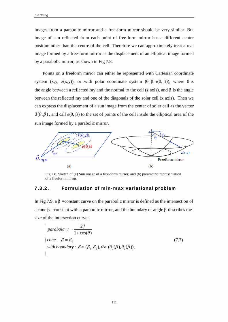
Lin Wang
111
images from a parabolic mirror and a free-form mirror should be very similar. But
image of sun reflected from each point of free-form mirror has a different centre
position other than the centre of the cell. Therefore we can approximately treat a real
image formed by a free-form mirror as the displacement of an elliptical image formed
by a parabolic mirror, as shown in Fig 7.8.
Points on a freeform mirror can either be represented with Cartesian coordinate
system (x,y, z(x,y)), or with polar coordinate system (θ, β, r(θ, β)), where θ is
the angle between a reflected ray and the normal to the cell (z axis), and β is the angle
between the reflected ray and one of the diagonals of the solar cell (x axis). Then we
can express the displacement of a sun image from the center of solar cell as the vector
( , )s θ β, and call e(θ, β) to the set of points of the cell inside the elliptical area of the
sun image formed by a parabolic mirror.
Fig 7.8. Sketch of (a) Sun image of a free-form mirror, and (b) parametric representation of a freeform mirror.
7.3.2. Formulation of min-max variational problem
In Fig 7.9, a β =constant curve on the parabolic mirror is defined as the intersection of
a cone β =constant with a parabolic mirror, and the boundary of angle β describes the
size of the intersection curve:
1
0
1 2 2
2:1 cos( )
:: ( , ), ( ( ), ( )),
fparabola r
conewith boundary
θβ β
β β β θ θ β θ β
= + = ∈ ∈
(7.7)

Chapter 7 Single freeform reflector design for concentration photovoltaic
112
Fig 7.9. r(θ,β0) defines an intersection curve between mirror and a cone with half angle β0.
From energy conservation Eq. (7.8), the irradiance of a single elliptical sun image on
solar cell can be deduced as:
| ( , ) | cos ( , ) ( , ) ( , ) ( , )| ( , ) | cos ( , )( , )
( , ) ( , )
sun cell
suncell
E J d d E a bE J d dE
a b
θ β φ θ β θ β θ β π θ β θ βθ β φ θ β θ βθ βπ θ β θ β
=
⇒ = (7.8)
Where Esun is a constant 900w/m2, or is also defined as 1 sun, | ( , ) |J d dθ β θ β is the differential area on a mirror,
( , )φ θ β is the angle between incident ray and normal vector of reflector, a(θ,β), and b(θ,β) are mayor and minor semi-axes of an elliptical image.
Under close fit parabola approximation, these quantities can all be calculated
from a parabolic mirror, and the irradiance of an elliptical sun image is finally
deduced. To take into account the displacement induced by a freeform mirror, here we
define the stepped function K,
1 ( , )( , , )
0 ( , )cell
cellcell
r eK r
r eθ β
θ βθ β
∈= ∉
(7.9)
where e(θ,β) is the elliptical region that would be illuminated by the parabolic mirror defined before, shown in Fig 7.8(a), and cellr gives the displacement vector of the ellipse on solar cell. With the aid of previous defined quantities, irradiance distribution on solar cell can be deduced by integrating all these elliptical images:
| | cos( ) ( ( , ), , ) suncell cell
E JE r K r s d dab
φθ β θ β θ βπ
= −∫ ∫
(7.10)
In Eq. (7.10), the only unknown is the displacement function ( , )s θ β. In order to
achieve a uniform irradiance distribution on solar cell, we can summarize it as a min-
max variational problem [8] where the maximum irradiance on solar cell should reach
a minimum by varying unknown function ( , )s θ β.

Lin Wang
113
7.3.3. Integrability condition for displacement function
As we have seen in section 7.2.1 and section 7.2.2 that the placement of each elliptical
image is determined by its central ray. All central rays together form a planar incident
wave-front. If the reflected wave-front is spherical, then the mirror acquires a
parabolic shape. In this sense, displacement function ( , )s θ βactually defines a
different reflected ray-bundle. In order to guarantee that this reflected ray-bundle
defined by displacement function ( , )s θ β also forms a wave-front, or in other words,
to guarantee the C1 smoothness of freeform mirror, the displacement function ( , )s θ β
should fulfill the integrability condition. There are several equivalent formulations for
the integrability condition [9, 10]. Supposing that N
defines a vector field in R3 space,
the integrability condition states that:
0N N∇× = (7.11)
Since the function ( , )s θ βis defined on the plane of solar cell, it’s more convenient to
use the equivalent formulation based on the 2D etendue conservation condition:
2 0DEtendue dxdp dydq dzdr= + + = (7.12)
where (x,y,z) is the starting position of a ray and (p,q,r) are its direction cosines.
Since ( , )s θ β is defined at a plane with z = constant, then dz = 0, and we have:
2 0DEtendue dxdp dydq= + = (7.13)
Then this min-max variational problem can now be restated as a wave-front design
problem to achieve uniform irradiance distribution. As in ref [11], a simple wave-
front can be constructed by taking the rays passing through the x-axis, for which dy=0
and thus the integrability condition is just dxdp=0. This means that in this case,
direction cosine p=cos β is only a function of x coordinate (so the bundle in the x-p
plane has no area), and each fan of rays at a point x forms a cone shape whose axis is
the x-axis. As an example, Fig 7.10 shows an example of such a wave-front
construction on solar cell. Function ( , )s θ β in this example is reduced to ( )s β
which
can also be deduced easily from a given function r(β).

Chapter 7 Single freeform reflector design for concentration photovoltaic
114
Fig 7.10. Sketch of (a) Rotational wave-front around one given axis on solar cell and (b) its r(β) function.
7.3.4. Tangential condition
The tangent condition states that the image of acceptance angle cone should be inside
the cell, at most tangent to the boundary of the solar cell, as shown in Fig 7.11. If we
represent the reflector with function z(x,y), its normal vector at point (x,y,z) is then
given by ( , , 1)z zx y
∂ ∂−
∂ ∂. The variation of this normal vector is restricted by boundaries of
solar cell. Function ( , , , , ) 0z zF x y zx y
∂ ∂=
∂ ∂ defines the boundary of allowable normal
vector. This condition restricts the movement of the image of sun, making the
aforementioned min-max variational problem a constrained problem. From close fit
parabola approximation, the restriction on normal vector variation is equivalent to the
restriction on the displacement function ( , )s θ β.
Fig 7.11. Tangent condition: the movement of acceptance cone angle
should be inside the solar cell.
r(β)
cell
, , , , 0z zF x y zx y
∂ ∂= ∂ ∂
, , 1z zx y
∂ ∂= − ∂ ∂
N
( ), , ( , )P x y z x y=
a b a

Lin Wang
115
7.3.5. Numerical solution
As we have seen above that this min-max variationalal problem is subject to two
conditions: integrability and tangential condition, analytical solutions to this
variational problem has not been acquired yet. In this section, we are going to present
a numerical method based on design of incident and reflected wave-front. Basic
design steps are:
1. Selection of one input wave-front;
2. Design of one output wave-front;
3. Reflector construction from input and output wave-front.
The shape of mirror is calculated as a generalized Cartesian Oval calculation [10],
once incident and reflected wave-front are designed. Although in previous discussion
the selected ray-bundle contains all central rays, through which a planar wave-front
can be built, other selections are also possible. Fig 7.12 shows three types of selection.
Ray A and C reside at the edge of input ray-bundle, and are reflected to the edge point
A’ and C’ on the elliptical image. Ray B is the central ray as mentioned before. Fig
7.13 shows wave-fronts constructed from different types of selection. Planar wave-
front corresponds to the selection of central rays B, and Cone-type wave-fronts
correspond to the selection of rays A and C. Although these three selections are
equivalent to each other, the selection of A and C ray-bundle will provide certain
convenience to the second step of design of the output wave-front.
Fig 7.12. Selection of input ray-bundle

Chapter 7 Single freeform reflector design for concentration photovoltaic
116
Fig 7.13. Input Wave-front for selected ray-bundle.
As an example, a freeform mirror is calculated as a generalized Cartesian Oval to
transform wave-front C into a spherical wave-front, as shown in Fig 7.14.
Fig 7.14. Transformation from Wave-front C into a spherical wave-front
All elliptical images of acceptance angle cone have a common base point, which
is the center of reflected spherical wave-front. Within each big image of acceptance
cone is a sun image. All these sun images together contribute to the irradiance
distribution on solar cell. Fig 7.14 and Fig 7.15 show how an iso-β strip
(representation as r(θ,β0)) part of reflector contribute to the irradiance distribution on
solar cell. When β is close to its maximum value βmax, as shown in Fig 7.15(b), the
displacement is very limited in order to fulfill the tangent condition; however, when β
is smaller and smaller, the space for displacement becomes bigger, because the size of
image of acceptance angle cone is also smaller.

Lin Wang
117
Fig 7.15. Irradiance contribution from iso-β strips:
(a) β = 450 (b) β = 800 (c) β = 100
Based on designs shown in Fig 7.14 and Fig 7.15, we are going to present an
algorithm to deal with a degraded variational problem, where the displacement
function ( , )s θ β reduces to ( )s β
and the reference axis for angle β is the diagonal
direction. That means displacement for irradiance from an iso-β strip is the same
along the diagonal direction. As we have seen in Section 7.3.3, this type of
displacement function fulfills automatically the integration condition. The flow chart
of proposed algorithm is the following:

Chapter 7 Single freeform reflector design for concentration photovoltaic
118
Fig 7.16. Flow chart of numerical algorithm.
In Fig 7.16, the value of S(β i) is obtained by linear search. A maximum
irradiance value Emax is given first, and then S(β i) has to fulfill the condition that the
addition of displaced irradiance distribution with previous irradiance distribution:
max0
max( ( ( ), ))i
i ik
E r S Eβ β=
− <∑ (7.14)
In this way, the final irradiance distribution is designed to be smaller than Emax.
We can also reduce the target value of Emax step by step in order to approach to the
real solution to this Min-Max variational problem.
Design 1: A mirror is calculated by transforming wave-front C’ into a spherical
wave-front Wf1 with its center on the diagonal of solar cell.
Retrieve iso-β irradiance distribution with aid of design 1: E(β0), E(β1),… Ε(βn) (β0> βn).
Given Emax, S(β0)=0
Numerical Search of S(βi).
Construct a reflected wave-front Wf2 from displacement function S(β).
Next β
Design 2: A mirror is calculated by transforming wave-front C’ into a rotational
wave-front Wf2.

Lin Wang
119
7.4. Design Examples
In this section, two concentrators with acceptance angle ±0.90 and ±1.00 are designed.
In order to make design compact, each concentrator is designed as a solid lens with
bottom surface metalized, as shown in Fig 7.17. Due to material’s refractive index,
e.g.1.5, the acceptance angle is reduced inside the material to α/1.5.
Fig 7.17. Solid concentrator with a metalized bottom surface and square aperture.
Design parameters are listed in Table 7.1. Since the geometric concentration is
650X, in the most uniform case, average irradiance E1 on solar cell is 650 suns, or
0.65Mw/m2. However, taking into account the acceptance angle, average irradiance
on solar cell should always be higher than 0.65Mw/m2. As we will see in these two
design examples, bigger acceptance angle corresponds to high average irradiance.
Therefore, embedding the mirror surface into a solid module can effectively reduce
the acceptance angle to α/1.52, and reduce the average irradiance distribution on solar
cell. Table 7. 1 design parameters
Geometric Concentration Cg Solar cell Material index
650X 1×1mm2 1.52
Fig 7.18 and Fig 7.19 show simulation results of solid concentrators with
acceptance ±0.90 and ±1.00 respectively.

Chapter 7 Single freeform reflector design for concentration photovoltaic
120
Fig 7.18. Simulation result when sun is centred. (a) Peak irradiance is 1.41Mw/ m2 at 00 incidence (b) Peak irradiance 1.9Mw/m2 at 0.90 incidence (c) Transmission curve.
(a) 00 incidence
(b) 0.90 incidence
(c)
Sharp decrease
Slow decrease

Lin Wang
121
Fig 7.19. Simulation result when sun is centred. (a) Peak irradiance is 1.528Mw/ m2 at 00 incidence (b) Peak irradiance 3.59Mw/m2 at 0.90 incidence (c) Transmission curve.
For a typical parabolic reflector design, a sharp decrease of the transmission
curve beyond the acceptance angle can often be noticed, because the central hot spot
(a) 00 incidence
(b) 10 incidence
(c)
Sharp decrease
Slow decrease

Chapter 7 Single freeform reflector design for concentration photovoltaic
122
fade out from solar cell quickly. In Fig 7.18 and Fig 7.19, at normal incidence 00,
peak irradiances on solar cell are 1.41Mw/m2 and 1.528Mw/m2; at declined incident
angle, the peak irradiances have increased to 1.9Mw/m2 and 3.59Mw/m2, and two hot
spots can be observed at the boarder of solar cell. Increasing the incident angle can
finally “push” these hot spots outside the solar cell, causing a sharp decrease in the
transmission curve. Further increasing the incident angle only causes a slow decrease
in the transmission curve, due to the gradual fading out of irradiance distribution on
solar cell. These two transmission curve also demonstrate the successfulness of these
two designs in achieving uniform irradiance distribution on solar cell.
7.5. Conclusion
In this chapter, we have developed a new design concept to solve the uniformity
irradiance problem on solar cell. By making parabolic approximation of the design
problem, we have formulated this uniformity problem into a 2D min-max variational
problem. This variational problem is subject to two conditions: integrability and
tangential conditions. Then, we have developed a numerical algorithm to solve a
degraded 1D min-max variational problem. At the end, two solved examples with
650X concentration and ±0.90 and ±10 acceptance angle using numerical optimization
methods have been presented. The two transmission curves also reveal the effect of
uniform irradiance on solar cell.
References 1. Chaves, J., Introduction to Nonimaging Optics (CRC Press, 2008).
2. R. Winston, J.C. Miñano, P. Benítez, “Nonimaging Optics”, (Elsevier-Academic Press, New York, 2005)
3. http://en.wikipedia.org/wiki/Acceptance_angle_%28solar_concentrator%29
4. David G. Jenkins, "High-uniformity solar concentrators for photovoltaic systems", Proc. SPIE 4446, 52 (2001).
5. P. Benitez, and J. C. Miñano, “Concentrator Optics for the next generation photovoltaics”. Chap. 13 of A. Marti & A. Luque. Next Generation Photovoltaics: High Efficiency through Full Spectrum Utilization, (Taylor & Francis, CRC Press, London, 2004).
6. P. Benítez, J. C. Miñano, P. Zamora, R. Mohedano, A. Cvetkovic, M. Buljan, J. Chaves, and M. Hernández, “High performance Fresnel-based photovoltaic concentrator,” Opt. Express 18(S1), A25–A40 (2010).
7. M. Born, E. Wolf, “Principles of Optics”, (Pergamon, Oxford, 1975).

Lin Wang
123
8. L. Elsgoltz, “ecuaciones diferenciales y cálculo variacional” tercera edición, 1977.
9. Juan. C. Miñano, “Application of the conservation of etendue theorem for 2D subdomains of the phase space in nonimaging concentrators”, Applied Optics, Vol 23, No 12,1983.
10. R. K. Luneburg Berkeley, “Mathematical Theory of Optics”, CA: University of California Press, 1964.
11. Pablo Benitez, Ruben Mohedano Arroyo and Juan C. Minano, "Design in 3D geometry with the simultaneous multiple surface design method of nonimaging optics", Proc. SPIE 3781, 12 (1999).
12. Jorge Nocedal, Stephen J. Wright, “Numerical Optimization”-second edition, Springer, 2006

Chapter 8 Time-varying SMS optics
124
Chapter 8. Time-varying SMS optics
8.1. Introduction
Time-varying optics is used in multiple fields: adaptive optics for astronomy,
Advanced Front lighting Systems (AFS) in automotive, laser scanning displays, etc.
Recently, it has gain attention in solar applications, particularly in CPV [1-4]. In ref
[1], a lateral translating waveguide with micro structures is designed to track the sun
movement and transmit the sun energy to edge mounted solar cells. In Ref [2] and [3],
two lateral moving lens arrays concentrate sun energy to solar cells while tracking the
sun movement. In Ref [4], solar cell array follows a non-linear trajectory relative to
stationary lens array.
In this work, a new design concept of beam steering device capable of tracking
wide angular range is presented. We will focus on an afocal beam steering system,
which means that it converts an parallel input rays coming within the design angular
range into parallel output rays always in the same direction.
There are two types of designs depending if the source is to be tracked (Type I),
or the target (Type II). The first case, shown in Fig 8.1, can be applied, for instance, to
track the sun to make a natural lighting luminare and will be studied in this research.

Lin Wang
125
(a) (b)
Fig 8.1. Beam steering device with two lens arraysto track the source: (a) Normal incidence (b) Off-axis incidence
In Fig 8.1, each of lens arrays has one planar surface which effectively avoids the
appearance of “spurious” light mentioned in Ref [5]. The bottom lens array always
remains stationary, while the top lens array can be translated in both horizontal and
vertical direction during tracking. This configuration shown in Fig 8.1(b) is the
Galilean-type, because the bottom lens is placed before the focal point of the first lens;
while for the Keplerian-type, the bottom lens should be placed after the focal point.
For the same focal length of the first lens, the Galilean-type configuration is more
compact than the Keplerian-type configuration; therefore only Galilean-type
configuration will be investigated in this work. The advantage of this configuration
over other lateral moving optics [1-4] is that the 2 lens arrays can be designed and
mounted as an independent tracking module. Rear CPV or diffuser modules only need
to match the output specifications from previous tracking module. Systematic division
into different functional modules could potentially reduce the overall cost and
improve the system stability.
The main objective of this chapter is to develop an extended SMS method [7, 8]
capable to realize the described beam steering concept for a wide angular range, more
than 400 degrees. The design procedure will be applied to Type I systems (in which
the source is tracked), but can be easily extended to Type II ones. The performance of
a beam steering devices will be measured by its tracking angular range and
divergence of output rays. In laser applications [5, 6], the divergence of output rays is
required to be close to the diffraction limit. That requirement can be greatly relaxed
in solid state lighting and solar applications.
In Section 8.2, a straight-path moving optics will be presented to analyze its
tracking capability. In Section 8.3, a curve-path moving optics designed by the
extended SMS design procedures are described for wider angular range. Section 8.3.3

Chapter 8 Time-varying SMS optics
126
gives the results of 2D translational design, and Section 8.3.4 gives the 3D rotational
design results.
8.2. Straight-path moving optics in two dimensions
8.2.1. Design principles
Conventional way to design a beam-steering device is to use Keplerian or
Galilean telescope structures, comprising two lens elements, as shown in Fig 8.2.
Keplerian structure is made up of two converging lens sharing a common focal point
and Galilean structure has one top converging lens and one bottom diverging lens.
Supposing that the focal lengths of top and bottom lens are f1 and f2 respectively,
angular magnification “m” of a Keplerian structure is then defined as f1/f2. Another
magnification “M” is related with the width of input and output parallel rays, which is
reverse to the angular magnification.
At 00 incident angles, two lenses have a common optical axis to produce 00
output angle parallel rays; When incident angle increase to θ degrees, the bottom lens
remain fixed, while the top lens has to move horizontally a distance ∆x, making the
output angle unchanged, as shown in Fig 8.2(b) and Fig 8.2(d). Movement ∆x can be
calculated as the image height on the focal plane of the top lens: 1x f tgθ∆ = .

Lin Wang
127
Fig 8.2. Sketch of Kepleiran and Galilean type beam steering devices.
It’s clear that for the same angular magnification value, Galilean type structure is
more compact than Keplerian structure. In the following discussion, we are going to
concentrate on the Galilean type beam steering devices. As shown in Fig 8.1, in order
to increase the transmission efficiency of array optics, stray rays or spurious rays
should be avoided by using two planar surfaces on each lens array.
The size of top lens and bottom lens should be equal to make lens arrays. Now
we are going to calculate the maximum incident angle θmax to guarantee 100%
transmission efficiency. The bottom lens is always fixed and the top lens moves
horizontally according to the incident angle. The size of top and bottom lens is the
same represented as dtop. The width of output parallel ray-bundle is:
2
1bottom top top
fd d M df
= = (8.1)
At maximum incident angle θmax, the output rays touch the boarder of the bottom
lens, as shown in Fig 8.3. This condition can be expressed as:
2
12 2topbottom dd fx
f+ ∆ ⋅ = (8.2)

Chapter 8 Time-varying SMS optics
128
Where 1 maxx f tgθ∆ = . Simplifying this equation gives the θmax as:
1 1max
2 1
(1 )[ (1 )] [ ]2 2
top topd d Mtg M tgf f M
θ − − −= − == (8.3)
Fig 8.3. Calculation of maximum incident angle θmax.
In equation (8.3), the width magnification M should be always smaller than “1”
in order to fulfill the lossless requirement. Fig 8.4 shows design parameters of top
and bottom thin lenses, whose radii are R1 and R2 respectively. The thickness of each
lens, t1 and t2, are selected much smaller than the distance between two lenses, so that
their focal lengths can be calculated by lens-maker’s equation [1]: 1
1topRf
n=
− and
2
1bottomRf
n= −
−.
Fig 8.4. Thin lenses Galilean structure design.
R1 R2
(a) Top lens (b) Bottom lens
t2 t1

Lin Wang
129
8.2.2. Design example
Table 8.1 gives specifications of a design with angular magnification 5 or width
magnification 0.2. Artificial material with refractive index 1.5 is used for the top and
bottom lenses.
Table 8.1. Specifications
Top Lens’ central thickness
Bottom lens’ central thickness R1 M
Size of lens element θmax
2mm 2mm 10mm 0.2 6mm ±450
The radius for top lens R1 is given as 10mm. From section 8.2.1, we can
determine that the radius of bottom lens R2 should be 2mm in order to achieve the
given angular magnification. The distance between two lenses is approximately
13.3mm to make them telescopic. The bottom lens’ profile is set as a parabola in
order to extend to full size 6mm. We can calculate that the maximum incident angle
θmax should be 310 degrees, based on Eq. (8.3).
Fig 8.5. Simulation results of straight-path moving optics.
The straight-path moving optics fails to track incident rays at a large incident
angle, due to undesired caustics between 2 lenses, as shown in Fig 8.5. When incident
angle is greater than 100, the field curvature of the first lens makes it impossible to
place the top lens properly by only horizontal movement. The calculation in Section
8.2.1 only considers the first order property of the system, without taking into account
(a) (b) (c) (d)
θ= 00 θ =100 θ =200 θ =300

Chapter 8 Time-varying SMS optics
130
high order aberrations of the top lens. These uncontrolled effects results in lower
transmission efficiency and many stray rays inside the beam steering device.
8.3. Curve-path moving optics in two dimensions
In order to remove undesired effects happened in straight-path design and further
extend the tracking angle range to more than 400 degrees, curve-path tracking
trajectory has to be permitted. Let’s consider that the bottom lens is fixed and the top
lens can move freely. Curve-path means the top lens can move in both horizontal
direction and vertical direction. As shown in Fig 8.1, the aperture stop of each array
element is placed at the front surface of the top lens in order to collect all incident
rays. At small incident angle, the field curvature produced by the top lens is relative
small, requiring only horizontal movement of the top lens; while at large incident
angle, from Seidel aberration theory, the field curvature increases in second order
respecting to the incident angle, which makes the pure lateral movement insufficient.
Also, it can be observed that during the movement of the first lens, the active part of
the bottom lens is moving from center to boarder. Considering the wide angular range
(more than ±400) within which two lens’ profiles have to work, this design problem is
an optimization problem of how to find optimum lens profiles that can have good and
balanced performance along the tracking trajectory. A good starting point is always
beneficial to locate a good local minimum. Based on these considerations, our design
procedure comprises 3 phases: calculation of the trajectory of the first lens and the
central profile of the bottom lens, the SMS construction of the top and bottom curves,
and further optimization with obtained lens profiles as a starting point. The first two
steps serve to provide a good initial design, which will be optimized in the third step.
8.3.1. Calculation of the trajectory
Since two planar surfaces of two lens arrays shown in Fig 8.1 is trivial to the
nature of this optical problem, but will complicate the explication of the design
principles, in the following discussion, we are going to neglect these two planar
surfaces, and suppose that the space between top and bottom curves is filled with a
fluid-like material to permit the movement of upper lens’ surface. At the final design
stage, two plane surfaces will be added. Also the Fresnel loss and material absorption
will not be considered.

Lin Wang
131
Here we propose two conditions for all the rays that pass through the center of the
aperture stop (which are also called “chief rays” in imaging systems) along the
tracking trajectory, as shown in Fig 8.6: the planar wave-front propagation and the
constant magnification around the chief ray. Since these two conditions usually
represent an afocal system, therefore we call these two conditions “central afocal
conditions”.
Fig 8.6. Central afocal conditions. (a) Sketch of the central part’s movement. (b) Definition of parameters (c) Planar wave-front propagation (d) Magnification definition.
In Fig 8.6(b), P1 is the center point of the top curve, which moves along the
tracking trajectory, and P2 is a point on the bottom curve. θ1 and θ2 are incident and
exit angles with respect to the normal vector at P1; θ3 and θ4 are incident and exit
angles with respect to the normal vector at P2. d is the distance between P1 and P2. R1
and R2 are curvature radii of the top and bottom curves. Because only the central part
of the top curve is considered, R1 remains constant along the tracking trajectory. The
wave-front propagation shown in Fig 8.6(b) can be formulated by generalized
Coddington equations for meridian wave-front [10]. In paraxial optics, the
magnification of an optical system is defined as a function of R1, d and R2 with the
small incident angle assumption; however in our case where the incident angle can be
far from the range of paraxial optics and the optical system is decentered, we have to
extend the magnification definition with incident and exit angles [11, 12]. With these
parameters, we can formulate the “central afocal conditions” into the following two
equations:
1 1 2 3 4 2,( 0, , , , , ; , ) 0out in n R d Rκ κ θ θ θ θ= = (8.4)
(b) (c) (d) (a)

Chapter 8 Time-varying SMS optics
132
1 1 2 3 4 2 0,( , , , , ; , ) out
in
xM n R d R Mx
θ θ θ θ = =
(8.5)
Where “n” is the material index between two curves. In these two equations, n, θ1, R1
and M0 are the input data. θ2, θ3 and θ4 can be determined easily from the ray path
shown in Fig 8.6(a). The two unknowns are “d” and “R2”, which can be solved
analytically from Eqs. (8.4) and (8.5):
0 1 3 42
2 1
(sec sec )sec sec
M R nRn
θ θθ θ
−=
− (8.6)
1 2 1 0 3 4
1 2
(cos sec cos sec )sec sec
nR Mdn
θ θ θ θθ θ
−=
− (8.7)
When θ1 is equal to 00 corresponding to the non-decentered position, θ2, θ3 and
θ4 are all equal to zero, and these two solutions are reduced into the paraxial solutions,
from which we can deduce analytically the central value of d and R2 at 00 incident
angle. The solution of “R2” in Eq. (8.6) gives the curvature distribution of the bottom
curve, which is an ordinary second order differential equation. Integration of this
differential equation gives the shape of the bottom curve. The solution of “d” in Eq.
(8.7) is then used to obtain the tracking trajectory of the top curve.
Although we have used constant magnification condition in the above deduction,
sometimes a varying magnification M (θ1) is more desirable. For example, if the
output bundle width is required to be constant at different incident angle, the
magnification function is:
01
1
( )cosMM θ
θ=
(8.8)
Where M0 is the magnification value at 00 incident angle. Solutions of “d” and “R2”
can be obtained by simply replacing M0 with M (θ1) in equations (8.6) and (8.7).
When two planar surfaces are added into this optical system, distance “d” in Fig
8.6(b) is further divided into 3 segments: the segment between two lenses and two
segments within each lens. In this case, analytical solution is hard to derive, but we
can solve these two central afocal conditions numerically.

Lin Wang
133
8.3.2. SMS construction of lens profiles
From the above procedure, the tracking trajectory and the central profile of the bottom
curve are calculated. Now, we are going to determine the shape of the top curve and
the boarder part of the bottom curve with the SMS method. The idea is to guarantee
100% collection efficiency and perfect control of rays at max incident angle θmax. The
SMS design procedures are illustrated in Fig 8.7:
(a) Parallel rays in the vertical direction are traced through central part of the
bottom curve to calculate the left part of the top curve. Since the outgoing rays
are parallel with angle θmax, the optical path length between the input wave-
front and the output wave-front should be constant, which enables us to
determine the shape of the top curve as a generalized Cartesian oval
calculation.
(b) The right part of the top curve is simply symmetrical to the left part.
(c) Parallel rays are traced through the right part of the top curve, and points on
the edge part of curve 2 are calculated also with constant optical path length
condition.
Fig 8.7. SMS design procedures.
Considering the symmetry of the optical system, the incident rays with –θmax
angle are also perfectly controlled by the SMS method. The size of the top curve
should be greater than the bottom curve in order to make an array. The primary
concern to determine this size is to guarantee 100% transmission at the maximum
incident angle. Of course, in practice small obscuration at the maximum incident
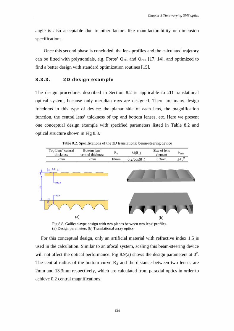
Chapter 8 Time-varying SMS optics
134
angle is also acceptable due to other factors like manufacturability or dimension
specifications.
Once this second phase is concluded, the lens profiles and the calculated trajetory
can be fitted with polynomials, e.g. Forbs’ Qbfs and Qcon [17, 14], and optimized to
find a better design with standard optimization routines [15].
8.3.3. 2D design example
The design procedures described in Section 8.2 is applicable to 2D translational
optical system, because only meridian rays are designed. There are many design
freedoms in this type of device: the planar side of each lens, the magnification
function, the central lens’ thickness of top and bottom lenses, etc. Here we present
one conceptual design example with specified parameters listed in Table 8.2 and
optical structure shown in Fig 8.8.
Table 8.2. Specifications of the 2D translational beam-steering device
Top Lens’ central thickness
Bottom lens’ central thickness R1 M(θ1) Size of lens
element θmax
2mm 2mm 10mm 0.2/cos(θ1) 6.3mm ±450
Fig 8.8. Galilean-type design with two planes between two lens’ profiles. (a) Design parameters (b) Translational array optics.
For this conceptual design, only an artificial material with refractive index 1.5 is
used in the calculation. Similar to an afocal system, scaling this beam-steering device
will not affect the optical performance. Fig 8.9(a) shows the design parameters at 00.
The central radius of the bottom curve R2 and the distance between two lenses are
2mm and 13.3mm respectively, which are calculated from paraxial optics in order to
achieve 0.2 central magnifications.
(a) (b)

Lin Wang
135
Fig 8.9. Performance analysis along the tracking trajectory with meridian rays.
To evaluate the optical performance, we measure the angular divergence [5, 6]
from the average ray direction of the output rays, and the deviation between the
average output direction and the vertical direction, as shown in Fig 8.10.
Fig 8.10. Definitions of divergence and deviation.
The SMS construction is carried out at 450 incident angle. In the design procedures
described in Section 8.2, central chief rays have been designed to have 00 exit angle
about the vertical direction; however, in an optimum case, the chief rays could have a
small deviation from 00 in order to make the average angular deviation as small as
possible. In Fig 8.11(a), the direct design by the SMS construction gives small angular
divergence and deviation values (all below 0.50). Then, two lens’ profiles and tracking
trajectory can be parameterized [17, 14] and optimized to correct the angular
deviation. Fig 8.11(b) gives the results of a design with optimized trajectory for which
there is a slightly higher angular divergence, but close to 00 angular deviations. Fig
8.11(c) compares the optimized trajectory (in red) with the direct calculation one (in
black). The similarity of these two trajectories before and after optimization implies
that the initial SMS design has provided a good starting point.
(a) (b) (c) (d)
θ1 = 00 θ1 = 150 θ1 = 300
θ1 = 450
Tracking trajectory

Chapter 8 Time-varying SMS optics
136
Fig 8.11. Angular divergence and deviation. (a) SMS construction without optimization (b)After optimization (c) Optimized tracking trajectory.
8.3.4. 3Dotational design example
In this section, optical performance of rotational lenslets generated directly from the
above optimized lens profiles is analyzed with meridian and skew rays, as shown in
Fig 8.12.
(a) (b)
(c)
Before optimization
After optimization

Lin Wang
137
Fig 8.12. Performance analysis of rotational lenslet with meridian and skew rays. (a) On-axis position (b) 200 position (c) 450 position with TIR reflection for boarder skew rays (d) Angular divergence and deviation.
At on-axis position in Fig 8.12(a), similar angular divergence as 2D design is
obtained, because only meridian rays contribute to the calculation. At off-axis
positions like Fig 8.12(b) and Fig 8.12(c), the astigmatic aberration caused by the top
lens increases rapidly with the incident angle, making it difficult for the rotational
bottom lens to redirect incoming rays into parallel exit rays. Some skew rays suffer
TIR reflection at the exit surface of the bottom lens, as shown in Fig 8.12(c), causing
undesired stray rays and reducing the transmission efficiency.
In order to reduce the angular divergence caused by the top lens’ astigmatic
aberration, one possibility keeping the rotational symmetry would be to re-design the
trajectory considering not only the tangential curvatures but the sagittal ones, and
minimizing the Gaussian curvature of the output wave-front. Another option consists
in re-designing the bottom lens as freeform. Free-form surface in general provides
more design freedoms, but complicates the surface’s design and fabrication. In this
case, the top lens is the same rotational symmetric lens, through which all the rays are
converged to a relative small area of the bottom lens, as shown in Fig 8.12. Therefore,
(a) (b)
(c) (d)
00
Front
Side
Front
Side
450
200
TIR

Chapter 8 Time-varying SMS optics
138
we propose another afocal condition for sagittal rays close to the central chief ray to
determine this freeform surface, with the assumption that sagittal rays only impinge
on the part of bottom surface close to the meridian plane. Since the distance between
two lenses has been determined in the 2D calculation, the only unknown is the sagittal
curvature of this freeform surface, as shown in Fig 8.13. This additional afocal
condition guarantees that sagittal rays close to the chief ray are redirect into parallel
exit rays in the vertical direction, which can be formulated similarly as Eq. (8.4) by
the generalized Coddington equations for sagittal wave-front [10]. In Fig 8.13(b),
along the meridian profile of the bottom curve, sagittal curves with calculated central
sagittal curvature are generated with the additional afocal condition. Then a freeform
surface is patched from these sagittal curves.
Fig 8.13. Freeform surface design condition.
Fig 8.14 shows the analysis results for freeform bottom surface. Comparing with
the rotational design in Fig 8.12, the freeform bottom surface significantly reduces the
angular divergence and increases the transmission efficiency at large incident angles.
However, there are still some skew rays that impinge on the border of the freeform
surface and suffer TIR reflection, because the “close to meridian plane” assumption is
not valid for these skew rays. In our future work, this freeform surface can be used as
a starting point for further optimization.
Sagittal rib curves
(a) (b)

Lin Wang
139
Fig 8.14. Performance analysis of lenslet with freeform bottom surface (a) On-axis position (b) 400 position without TIR reflection (c) 450 position with TIR reflection for boarder skew rays (d) Angular divergence and deviation.
8.4. Conclusions
In this work, we have firstly introduced straight-path moving optics and its limitations,
and then presented a new beam-steering design concept with potential applications for
sun tracking. The central part and tracking trajectory of this compact Galilean-type
array optics is determined by two central afocal conditions, and the boarder parts are
constructed by an extended SMS algorithm. Then the initial design is optimized with
standard optimization routines to find a better local minimum. Simulation results of
the 2D translational design demonstrate that meridian rays are well-controlled with
output angular divergence less than 0.50. In 3D analysis, rotational bottom surface is
proved to be not sufficient in controlling the skew rays, and freeform bottom surface
has to be implemented. We have introduced an additional afocal condition to
determine this freeform surface. The simulation results show that freeform surface has
(a) (b)
(c) (d)
400
00
450
Front view
Front view
Front view Side view Side view
Side view

Chapter 8 Time-varying SMS optics
140
significantly reduced the angular divergence from to around 10. In our future work,
optimization starting from designed freeform surface will be studied.
Reference
1. J. Hallas, J. Karp, E. Tremblay, and J. Ford, “Lateral translation micro-tracking of planar micro-optic solar concentrator,” Proc. SPIE 7769, 776904 (2010).
2. W. Sweatt, B. H. Jared, G. N. Nielson, M. Okandan, A. Filatov, M. B. Sinclair, J. L. Cruz-Campa, and A. L. Lentine, “Micro-Optics for High-Efficiency Optical Performance and Simplified Tracking for Concentrated Photovoltaics (CPV),” in International Optical Design Conference, OSA Technical Digest (CD) (Optical Society of America, 2010), paper ITuC4.
3. Fabian Duerr, Youri Meuret, and Hugo Thienpont, “Tracking integration in concentrating photovoltaic using laterally moving optics,” Opt. Express 19, A207-A218 (2011).
4. P. Kotsidas, E. Chatzi, and V. Modi, “Stationary nonimaging lenses for solar concentration,” Appl. Opt. 49, 5183–5191 (2010), http://www.opticsinfobase.org/abstract.cfm?URI=ao-49-27-5183.
5. E. Watson, “Analysis of beam steering with decentered micro-lens arrays,” Opt. Eng. 32, 2665–2670 (1993).
6. J. Gibson, B. Duncan, E. Watson, and J. Loomis, “Wide-angle decentered lens beam steering for infrared countermeasures applications,” Opt. Eng. 43, 2312 (2004).
7. R. Winston, J.C. Miñano, and P. Benítez, with contributions of N. Shatz, J. Bortz, Nonimaging Optics, (Academic Press Elsevier, 2004), Chap. 8.
8. Chaves, J., Introduction to Nonimaging Optics (CRC Press, 2008).
9. M. Born and E. Wolf, Principles of Optics, (Cambridge University Press, 1999).
10. Orestes N. Stavroudis, The mathematics of geometrical and physical optics, (Wiley-VCH, 2006).
11. Bryan D. Stone and G. W. Forbes, “Characterization of first-order optical properties for asymmetric systems,” J. Opt. Soc. Am. A 9, 478-489 (1992).
12. R. K. Luneburg, Mathematical Theory of Optics, (University of California Press, 1964).
13. G. W. Forbes, “Shape specification for axially symmetric optical surfaces,” Opt. Express 15, 5218-5226 (2007).
14. G. W. Forbes, "Robust, efficient computational methods for axially symmetric optical aspheres," Opt. Express 18, 19700-19712 (2010).
15. W. H. Press, S. A. Teukolski, W. T. Vetterling, and B. P. Flannery, Numerical Recipes in C++: The Art of Scientific Computing, Second Edition (Cambridge University Press, 2002).
Conclusions and future lines
141
Conclusions and future lines of investigations
1. Conclusions
The first part of this thesis (Chapters 2 to 5) is dedicated to the research and
development of SMS method in two dimensions and in three dimensions with
application to imaging optics.
In Chapter 2 we have advanced the state of the art SMS rotational spherical designs
for imaging applications, in which we choose up to four couples of input and output
meridian-ray bundles (called SMS-4M algorithm) as there are surfaces of the optical
system to be designed. A novel SMS construction procedure has been developed
based on optimizing parabola sections as the SMS incremental segments instead of
performing the standard SMS generalized Cartesian oval calculation. This approach
has itself improve the stability of the profile construction, but it has been found that
the C2 continuity of the profiles (which is not required in the SMS method) is even
more crucial. In comparison with the aplanatic designs, once a maximum spot radius
in the field is fixed, the SMS design has a wider FOV (the FOV diameter of the SMS
design is 1.42 times that of the equivalent aplanatic designs for the two-surface
design). In the four-surface SMS design case, we have shown that the selection of
design rays among the meridian rays of the FOV give good control of the image
formation quality only for meridian rays but not good enough to control of the
remaining rays.
Chapter 3 has been devoted to the comparison of the SMS-3M algorithm and SMS
1M-2S algorithm for three rotational aspheres. The SMS 1M-2S and SMS 3M
algorithms are then applied to a monochromatic objective design to compare their
control capability over all the rays in the phase space, or their imaging ability. Results
have shown that by selecting ray-bundles which spread uniformly in phase space,
SMS 1M-2S design has a more uniform RMS3D distribution. However compared to
SMS 3M design, it still has less control of RMS spot size over all fields of view,
especially the center field of view.
In Chapter 4 we have presented an SMS based optimization strategy for rotational
optics, which consists of two design phases. In the first phase, the optical system is
considered as monochromatic. The SMS method, which does not restrict the surface

Lin Wang
142
asphericity or system paraxiality, is embedded in an optimization process of the free
parameters (vertex positions, etc), so the SMS procedure repeated in every iteration,
being the SMS a very efficient way to represent complex aspherics. In the second
phase, the SMS monochromatic design is used as a starting point (after a fitting to
Forbs’ radial polynomials) for further monochromatic or polychromatic optimization
in commercial optical software. We have applied this design strategy to two
monochromatic ultra-compact SWIR camera designs, called RXXR and XRXR. The
landscape plot of merit function versus central vertices demonstrates that the merit
function is less sensitive to vertex positions than the central curvature of front surface.
Finally, starting from the concave type monochromatic design, an ultra-compact well-
corrected achromatic RXXR and XRXR designs with one added small lens at the exit
is found.
At the end of this section, in Chapter 5, we have introduced the application of SMS
3D to design of free-forms for imaging. We have explored eight types of two mirror
configuration, combining a first phase optimization of several parameters as in
Chapter 4 for the rotational case, and the second phase of further optimization, using
the free-form Forbs polynomials. Like in the rotation case, the SMS3D design method
combined with optimization process demonstrates to be an effective and fast way in
finding local optimum with reduced amount of parameters.
Summarizing, as demonstrated in chapters 2 to 5, the advantages of SMS method over
other optical design methods include:
• Designs with wide fields of view when SMS points are well selected;
• Flexible ray-bundles selection: meridian rays and skew rays;
• Drastic reduction of variables in the first stage optimization, where only free parameters is considered;
• Great potential to provide initial designs for rotational and freeform systems close to a good local minimum.
The second part of the thesis has been devoted to non-imaging applications. Chapter 6
has shown a metal-less plastic device which comprises of a collimation optics and
freeform micro lens array, capable of highly efficiently provide an excellent solution
to a complex design problem. In the collimation part, although the first grooved
mirror reversed the skewness of impact rays, the second grooved mirror was found to
have cancelled that reversal and formed a good far field image of the light source. The

Conclusions and future lines
143
microlens array was responsible of changing the angular aspect ratio of the beam
crossing it from 1:1 to 16:9 without changing its spatial distribution. This is easily
achieved by applying an etendue squeezing technique and each micro lens has two
SMS3D freeform surfaces designed for different horizontal and vertical magnification.
The final simulated transmission efficiency from light source to target area can reach
up to 86.75%.
Chapter 7 explained a single freeform mirror design capable of producing uniform
irradiance on solar cell. The design problem has been formulated as a min-max two
dimensional variation problem. Based on the geometric insight of this illumination
design, we have simplified the 2-D variation problem to a 1-D variation problem and
found its numerical solution with optimization method, leading to a novel freeform
solution. Selected examples demonstrated peak irradiances below 1,500 suns uniform
irradiance had been achieved for a compact 650X concentrator with ±10 degree
acceptance angle, which imply great improvements over the equivalent parabolic
concentrator.
Finally, in Chapter 8, a novel design concept of moving array optics has been
presented. We have developed an analytical method to determine an initial tracking
trajectory and extended the top and bottom lens’ surfaces with the SMS method.
Analysis results of a cylindrical model showed excellent performance (in terms of
diverge and deviation within ±450 angular range) which could be even further
improved by using parametric optimization of the curved tracking trajectory., a
Further research on a rotational model has shown that skew rays can be better
controlled by introducing a freeform surface on the secondary.

Lin Wang
144
2. Future lines of research
The future lines of work are summarized in the following table:
Rotational optics Freeform optics
Imaging • Development of SMS 4S algorithm • Extend SMS algorithm to more than 4 surfaces • Include zoom designs and wavelength
considerations
• Development of SMS design method with pupil discretization
• Investigate more freeform aberration theories, find new applications and study its manufacturability
Non-imaging
• Study the manufacturability of grooved freeform surface
• Research of AFS (advanced front lighting system) with time-varying SMS optics

Appendix A
145
Appendix A. Surface construction using Cubic Local Patches (CLP)
A.1 Statement of the problem
To design a freeform optical system, usually points and normal vectors on the optical
surfaces are firstly calculated based on design principles, and then polynomial
functions could be fitted to this given point cloud. But traditional fitting or
approximation methods becomes less effective in 3D design. In this report, a local
cubic patch (CLP) method is developed on this purpose. This method can fit a local
cubic patch at each n×m array of data, (n,m ≥4 ). The whole surface is made up of
local patches array. The advantage of this method is that it employs polynomials of
only degree 3, and makes use of both fitting and approximation in local patch
calculation. Thus the method has good properties like simple, fast, stable and accurate
to our needs.
A.2 CLP algorithm
Let’s consider first a simple patch with 4×4 poins, each of which has a pre-determined
normal vector, as shown in Fig A.1. As a local construction method, the CLP method
only makes use of the local points-array to calculate one patch. Each local cubic patch
has 16 (4×4) control points. Of course, it is desirable to be able to find a surface that
pass through all points position meanwhile has the given normal vectors, but in
practice the design freedoms which are those control points restrict the number of
conditions to be imposed. In this CLP algorithm, a compromise has been made

Lin Wang
146
between the interpolation of point positions and the fulfillment of normal vectors, so
that the constructed local patch should fulfill:
Fig A.1. Sketch of a local point array.
a. Having given positions and normal vectors on four corner points Q00, Q03, Q30,
Q33, and N00, N03, N30, N33
b. Approximating the position of other inner points to determine the inner control
points.
Given normal vectors on four corners, it’s convenient to select for each corner
point two perpendicular tangent vectors T and B to define a tangent plane, as shown
in Fig A.1. Based on the representation of NURBS [9], the calculation of a local patch
can be simplified to firstly calculate the control points on 4 boundary curves, and then
calculate the inner control points of the patch.
(1) Boundary curve
For example, one boundary curve with given data, Q00, N00, Q01, Q02, Q03, N03, in
Fig 1 ; The control points to be calculated are P00, P01, P02 , P03. To guarantee the first
requirement, Q0 and Q3 should be the end control points of the curve, and P01, P02
should on the tangent direction from P00 and P03. Then we can write:
00 00
03 03
01 00 0 00 0 00 00 00 00 00 00 00
02 03 1 03 1 03 03 03 03 03 03 03
, ,
, ,
P Q
P Q
P P T B T N B N T B
P P T B T N B N T B
α β
α β
=
=
= + + ⊥ ⊥ ⊥ = + + ⊥ ⊥ ⊥
(A.1)
Where Ti and Bi are unit tangent directions and αi and β i are the length along tangent
directions. Written in this format, there are 4 unknowns: α0, β0 and α1, β1. To best

Appendix A
147
approximate points Q01 and Q02 and using the NURBS curve representation, the
equations are following:
0,3 1 00 1,3 1 01 2,3 1 02 3,3 1 03 01
0,3 2 00 1,3 2 01 2,3 2 02 3,3 2 03 02
( ) ( ) ( ) ( )
( ) ( ) ( ) ( )
N u P N u P N u P N u P Q
N u P N u P N u P N u P Q
+ + + →
+ + + →
(A.2)
Where u1 and u2 are parameters that corresponds to point Q01and Q02 with arc length
parameterization [9]. Equation system (A.2) contains 6 linear equations with 4
unknowns, which is a typical least square approximation problem [9]:
6 4 4 1 6 1
0 0 1 1
min || ||
, , , x
t
N x q
x α β α β
× × ×−
= (A.3)
Simply transformation of Eq. (A.3) can lead to a matrix form with solution:
1( )
T T
T T
N Nx N qx N N N q−
=
⇒ = (A.4)
(2) Inner control points
With method in section A.1, we have calculated 12 boundary control points. What
remain to be calculated are 4 inner control points (P11, P12, P21, P22), with
requirements to best approximate 4 inner points and satisfy the boundary continuity
conditions. To this end, we can put these inner control points on the tangent plane of
adjacent corner points, as shown in Fig A.2:
P11 on the tangent plane of Q00;
P12 on the tangent plane of Q03;
P21 on the tangent plane of Q30;
P22 on the tangent plane of Q33;

Lin Wang
148
Fig A.2. Calculation of inner control points. Therefore we can write these inner control points in the following form with 8
unknowns:
11 00 0 00 0 00
12 03 1 03 1 03
21 30 2 30 2 30
22 33 3 33 3 33
0 0 1 1 2 2 3 3 , , , , , , , t
P P T B
P P T B
P P T B
P P T B
x
α β
α β
α β
α β
α β α β α β α β
= + +
= + +
= + + = + +
=
(A.5)
With these representations, this patch surface’s NURBS representation is given as
( , , )S x u v . Similar to the calculation of boundary curve, we can find a solution x
to
best approximate the inner point positions (Q11, Q12, Q21, Q22), which is another least
square approximation problem with simple solution:
11 11 11
12 12 12
21 21 21
22 22 22
( , , )
( , , )
( , , )
( , , )
S x u v Q
S x u v Q
S x u v Q
S x u v Q
→
→
→ →
(A.6)
Since only positions of four corner points are exactly interpolated, and other inner
points are only approximated, this cubic patch algorithm can also be extended to
include more inner points, or n×m point array (n>4, and m>4). The only change in the
above algorithm is to include more linear equations for fixed number of unknowns,
which can be solved use the least square approximation method. With this algorithm,

Appendix A
149
the normal directions on 4 given corners are preserved; the distance between given
points and surface are optimized; adjacent patches are jointed with good continuity.
Reference
9. L. Piegl, W. Tiller. The NURBS Book ,Springer-Verlag, Berlin, 2nd Ed, 1997.

Appendix B
150
Appendix B. SMS3D skinning with scaled initial patch
B.1 Statement of the problem
In SMS3D design procedures, skinning is the last process to construct from calculated
point cloud a suitable surface [9]. As described in the introduction Section 1.2, point
cloud for each freeform surface is obtained from several SMS chains with given
normal vectors. From mathematical point of view, there exist many interpolation
surfaces through given point cloud [11]. Generally speaking, a dense point cloud can
provide more surface information and specify the interpolation surface better than
sparse point cloud. In thesis of Blen [9], a skinning algorithm has already been studied,
as shown in Fig B.1, which comprises:
Fig B.1. SMS skinning algorithm.
a) A simple “lofted” patch ∑1 with order 3 is constructed between two adjacent
SMS chain curves R0 and R2;

Appendix A
151
b) Other ∑ i surfaces (i≠1) are calculated iteratively as generalized Cartesian
Ovals.
However, later study has found that simple “lofted” patch in this skinning
algorithm doesn’t works well for complex surface shape, e.g. saddle surface. In this
appendix, a new initial patch calculated from scaled SMS chains is going to be
presented.
B.2 Design parameters of two freeform mirrors
Fig B.2 illustrates design parameters of two free-form mirrors, which make up an
imaging system. The selection of these parameters is quite arbitrary without loss of
generality. The object plane is a square of 6×6mm2 on the X-Z plane with its center
located at (0,0,0), and the image plane is 18×18mm2 on the X-Y plane with its center
placed at (0,40,60). Therefore the magnification of this imaging system is 3.
Obscuration between two mirrors is also avoided. Poe and Soe are two initial points
on these two mirrors in order to determine their relative positions.
Fig B.2. Sketch of design parameters.
In this imaging system, the corresponding mapping between object plane and
image plane is shown in Fig B.3. The SMS construction routine is to use two pairs of
image and object wave-fronts, in this case (Obj1 ↔Img1) and (Obj2 ↔Img2), to
design initial curves, and another two pairs (Obj3 ↔Img3) and (Obj4 ↔Img4) to
obtain SMS ribs.

Appendix B
152
Fig B.3. Mapping between object plane and image plane.
However, this direct construction provides only a sparse point cloud with less
surface information, we are going to generate more points by SMS skinning.
B.3 Skinning procedures
Instead of using those 4 pairs of edge object and image points, we can also use
other inner points. We have found that when object points are closer to each other,
generated point clouds for two mirrors’ surface are also denser. These inner pairs of
object and image points can be easily obtained by scaling from those edge points
respecting to their center. Fig B.4(a) shows 4 scaled object points with scale factor 20.
Corresponding image points will be also scaled to have the same system
magnification. In Fig B.4(b), black points are points on mirror 1 generated with
scaled object and image points, and red points are generated by un-scaled object and
image points.
Fig B.4. Surface construction with scaled pairs of object and image points.
x
z
Obj_scale1
Obj_scale2
Obj_scale3 Obj_scale
4
0.3mm
Mirror 1
(a) Scaled object points (b) Point cloud on Mirror 1

Appendix A
153
It can be seen that these two point clouds coincide very well to each other, which
implies that for a good imaging system, mirror’s shape doesn’t change much with
different pairs of object and image points. Therefore, we can use this black point
cloud to fill in the space between two red boundary curves, as show in Fig B.5. The
calculation of initial patch through given point cloud follows the NURBS surface
interpolation routine [11].
Fig B.5. Initial patch on mirror 1 through black point cloud.
Once initial patch is obtained, other patches are then calculated with un-scaled
object and image points, as shown in Fig B.6. In order to check the surface quality, we
traced rays from designed object points, and then calculated the RMS spot diameter
on the image plane. In this example, 0.2um spot diameter has been achieved which
demonstrates the viability of presented skinning method.
Fig B.6. Skinned mirror surfaces and its simulation result.
Although this skinning method is capable to achieve very small RMS spot size
with many patches, the continuity between patches is not guaranteed in the design
Patch ∑1
Patch ∑1
Image plane
Object plane
(a) Patch surfaces (b) Simulation

Appendix B
154
procedures. That’s to say if we interpolate one single surface to each mirror, the
quality of interpolated surface can be worse than original patches due to the continuity
problem. Further improvement to the calculation of initial patch is still necessary with
additional smoothness constrain.
Reference
10. José Blen Flores, Doctoral Thesis “Design of multiple free-form optical surfaces in 3D” E.T.S.I.Telecomunicación, (2007).
11. L. Piegl, W. Tiller. The NURBS Book ,Springer-Verlag, Berlin, 2nd Ed, 1997.

Appendix A
155
Publications
Journal Papers
1. J.C. Miñano, Pablo Benitez, Lin Wang. An application of the SMS method for imaging designs. Optics Express, Vol. 17, Issue 26, pp. 24036-24044 (2009)
2. Lin Wang, Pablo Benítez, Juan C. Miñano, José M. Infante, Guillermo Biot, and Marta de la Fuente, "SMS-based optimization strategy for ultra-compact SWIR telephoto lens design," Opt. Express 20, 9726-9735 (2012)
Conference Proceedings
1. J.C. Miñano, Pablo Benitez, and Lin Wang, “Overview of the SMS design method applied to imaging optics”, Proc. SPIE 7429, 74290C (2009)
2. Jose M. Infante Herrero, Fernando Muñoz, Pablo Benitez, Juan Carlos Miñano, Lin Wang, Juan Vilaplana, Guillermo Biot and Marta de la Fuente, "Novel fast catadioptric objective with wide field of view", Proc. SPIE 7652, 765223 (2010)
3. Lin Wang, Pablo Benítez, J. C. Miñano, José Infante and Guillermo Biot, "Progress in the SMS design method for imaging optics", Proc. SPIE 8128, 81280F (2011)
4. Lin Wang, Pablo Benítez, J. C. Miñano, Jose Infante, Marta de la Fuente and Guillermo Biot, "Solid Catadioptric telephoto lens design with SMS method", Proc. SPIE 8167, 81670O (2011)
5. Jose M. Infante Herrero, Marta C. de la Fuente, Lin Wang, Juan Carlos Miñano Dominguez, Pablo Benítez, Guillermo Biot, Hammed Ahmadpanahi and Andres F. Cifuentes, "Design of a compact objective for SWIR applications", Proc. SPIE 8167, 81670K (2011)
6. Jose M. Infante Herrero, Juan Carlos Miñano Dominguez, Pablo Benítez, Guillermo Biot, Hammed Ahmadpanahi, Lin Wang, JiaYao Liu, Julio C. Chaves and Marta C. de la Fuente, "Imaging system applications of multichannel configuration", Proc. SPIE 8167, 81670L (2011)
7. Lin Wang, Pablo Benítez, J. C. Miñano, “Two freeform mirror designs with SMS3D”, freeform optics incubator meeting, Washington (2011)
8. Lin Wang, Pablo Benítez, J. C. Miñano, José Infante and Guillermo Biot, "Advances in the SMS design method for imaging optics", Proc. SPIE 8167, 81670M (2011)
9. Lin Wang, Pablo Benítez, J. C. Miñano, Jose Infante, Marta de la Fuente and Guillermo Biot, "Ultracompact SWIR telephoto lens design with SMS method", Proc. SPIE 8129, 81290I (2011)
10. Lin Wang, Pablo Benitez, and J. C. Miñano, “Beam-steering array optics designs with the SMS method”, Proc. SPIE 8485-04 (2012)

Publications
156