towards large-scale simulations of moving boundary ... · towards large-scale simulations of moving...
TRANSCRIPT
Towards Large-scale Simulations of MovingBoundary Problems in Compressible Flows using
OpenFOAM®:Challenges and Opportunities
A. Montorfano 1 F. Piscaglia 1 A. Onorati 1 S. M. Aithal 2
1Dipartimento di Energia, POLITECNICO DI MILANO
2Argonne National Laboratory, Lemont, IL 60439, United States
March 26, 2015
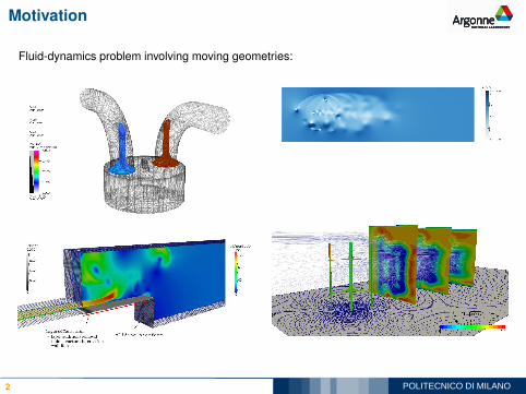
Motivation
Fluid-dynamics problem involving moving geometries:
2
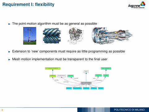
Requirement I: flexibility
◮ The point motion algorithm must be as general as possible
◮ Extension to ’new’ components must require as little programming as possible
◮ Mesh motion implementation must be transparent to the final user
Foam::engineTopoMesh
fvMesh
polyTopoChanger engineTimevalveBank
engineValves_
PtrList< engineValve >
engineDB_
topoChanger_
enginePiston
piston_
topoManager
topoMgr_
List< polyMeshModifierDefinition * >
fourStroke layeredTopoEngine simplePiston simpleValve twoStroke
3
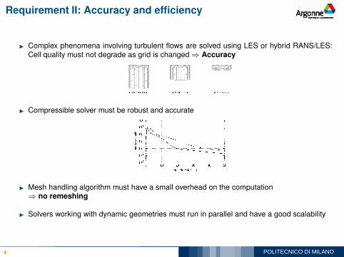
Requirement II: Accuracy and efficiency
◮ Complex phenomena involving turbulent flows are solved using LES or hybrid RANS/LES:Cell quality must not degrade as grid is changed ⇒ Accuracy
◮ Compressible solver must be robust and accurate
◮ Mesh handling algorithm must have a small overhead on the computation⇒ no remeshing
◮ Solvers working with dynamic geometries must run in parallel and have a good scalability
4
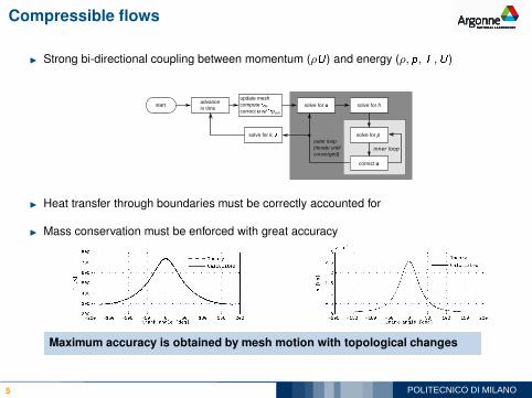
Compressible flows
◮ Strong bi-directional coupling between momentum (ρU) and energy (ρ, p,T ,U)
startadvance
in timesolve for u solve for h
solve for p solve for k, �
outer loop
(iterate until
converged)inner loop
correct u
update mesh
compute ✁M
correct u w/ ✂pcorr
◮ Heat transfer through boundaries must be correctly accounted for
◮ Mass conservation must be enforced with great accuracy
Maximum accuracy is obtained by mesh motion with topological changes
5
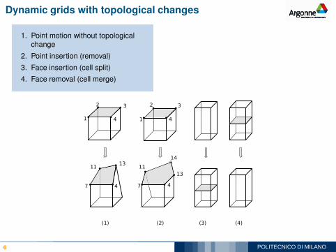
Dynamic grids with topological changes
1. Point motion without topologicalchange
2. Point insertion (removal)
3. Face insertion (cell split)
4. Face removal (cell merge)
(3) (4)
7
1113
4
1
2 3
4
(1)
1
2 3
4
7
11
14
13
4
(2)
6
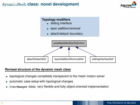
dynami Mesh class: novel development
Topology modifiers◮ sliding interface
◮ layer addition/removal
◮ attach/detach boundary
polyMeshModifierDefinition
attachDetachDef layerAdditionRemovalDef slidingInterfaceDef
Revised structure of the dynamic mesh class
◮ topological changes completely transparent to the mesh motion solver
◮ automatic case setup with topological changes
◮ topoManager class: very flexible and fully object-oriented implementation
7
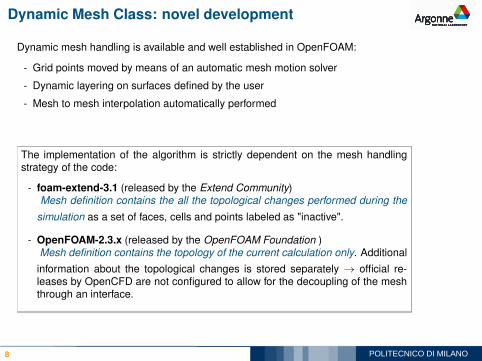
Dynamic Mesh Class: novel development
Dynamic mesh handling is available and well established in OpenFOAM:
- Grid points moved by means of an automatic mesh motion solver
- Dynamic layering on surfaces defined by the user
- Mesh to mesh interpolation automatically performed
The implementation of the algorithm is strictly dependent on the mesh handlingstrategy of the code:
- foam-extend-3.1 (released by the Extend Community)Mesh definition contains the all the topological changes performed during the
simulation as a set of faces, cells and points labeled as "inactive".
- OpenFOAM-2.3.x (released by the OpenFOAM Foundation )Mesh definition contains the topology of the current calculation only. Additional
information about the topological changes is stored separately → official re-leases by OpenCFD are not configured to allow for the decoupling of the meshthrough an interface.
8
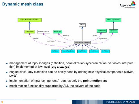
Dynamic mesh class
Foam::engineTopoMesh
fvMesh
polyTopoChanger engineTimevalveBank
engineValves_
PtrList< engineValve >
engineDB_
topoChanger_
enginePiston
piston_
topoManager
topoMgr_
List< polyMeshModifierDefinition * >
fourStroke layeredTopoEngine simplePiston simpleValve twoStroke
◮ management of topoChanges (definition, parallelization/synchronization, variables interpola-tion) implemented at low-level (topoManager)
◮ engine class: any extension can be easily done by adding new physical components (valves,ports)
◮ implementation of new ‘components’ requires only the point motion law
◮ mesh motion functionality supported by ALL the solvers of the code
9
slidingInterfa e
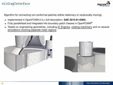
Algorithm for connecting non-conformal patches (either stationary or reciprocally moving).
◮ Implemented in OpenFOAM-2.3.x (full description: SAE 2015-01-0384).
◮ Fully parallelised and integrated into boundary patch classes in OpenFOAM®
◮ Tested on engineering geometries, including IC Engines, rotating machinery and on severalsimulations involving separate mesh regions.
10
slidingInterfa e
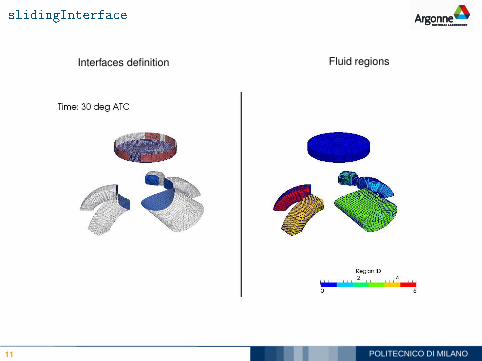
Interfaces definition Fluid regions
11
slidingInterfa e
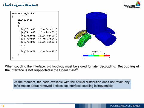
s avengingPorts
{
interfa es
XX
(
( ylPort01 inletPort01 )
( ylPort02 inletPort02 )
( ylPort03 inletPort03 )
( ylPort04 inletPort04 )
( ylPort05 inletPort05 )
...
...
( ylPortXX inletPortXX )
)
}
When coupling the interface, old topology must be stored for later decoupling. Decoupling ofthe interface is not supported in the OpenFOAM®.
At the moment, the code available with the official distribution does not retain anyinformation about removed entities, so interface coupling is irreversible.
12
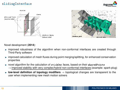
slidingInterfa e
Novel development (2014):
◮ improved robustness of the algorithm when non-conformal interfaces are created throughThird-Party software
◮ improved calculation of mesh fluxes during point merging/splitting, for enhanced conservationproperties
◮ novel algorithm for the calculation of sti kOut faces, based on their sharedPoints→ improved stability with very complex/hybrid non-conformal interfaces (example: spark-plug)
◮ low-level definition of topology modifiers → topological changes are transparent to theuser when implementing new mesh motion solvers
13
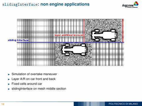
slidingInterfa e: non engine applications
◮ Simulation of overtake maneuver
◮ Layer A/R on car front and back
◮ Fixed cells around car
◮ slidingInterface on mesh middle section
14
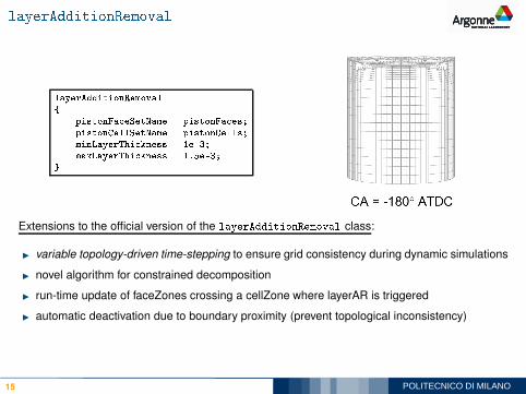
layerAdditionRemoval
layerAdditionRemoval
{
pistonFa eSetName pistonFa es;
pistonCellSetName pistonCells;
minLayerThi kness 1e-3;
maxLayerThi kness 1.5e-3;
}
Extensions to the official version of the layerAdditionRemoval class:
◮ variable topology-driven time-stepping to ensure grid consistency during dynamic simulations
◮ novel algorithm for constrained decomposition
◮ run-time update of faceZones crossing a cellZone where layerAR is triggered
◮ automatic deactivation due to boundary proximity (prevent topological inconsistency)
15
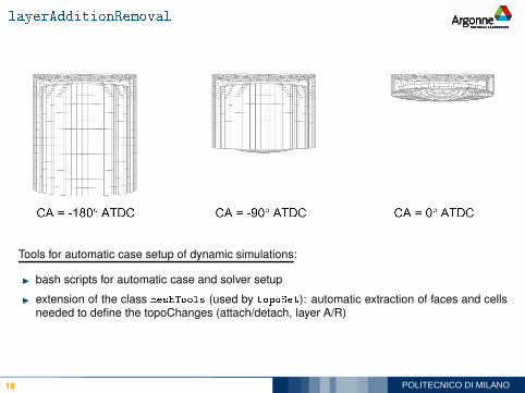
layerAdditionRemoval
Tools for automatic case setup of dynamic simulations:
◮ bash scripts for automatic case and solver setup
◮ extension of the class meshTools (used by topoSet): automatic extraction of faces and cellsneeded to define the topoChanges (attach/detach, layer A/R)
16
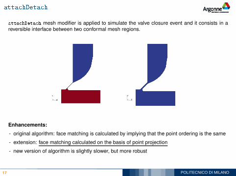
atta hDeta h
atta hDeta h mesh modifier is applied to simulate the valve closure event and it consists in areversible interface between two conformal mesh regions.
Enhancements:
- original algorithm: face matching is calculated by implying that the point ordering is the same
- extension: face matching calculated on the basis of point projection
- new version of algorithm is slightly slower, but more robust
17
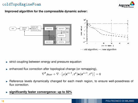
oldTopoEngineFoam
Improved algorithm for the compressible dynamic solver:
startadvance
in time
update mesh
compute �M
correct u w/ ✁pcorr
solve for u solve for h
solve for p
solve for k, ✂
outer loop
(iterate until
converged)
correct u
inner loop
- -: old algorithm; —: new algorithm
◮ strict coupling between energy and pressure equation
◮ enhanced flux correction after topological change (or remapping),
∇2
pcorr +∇ ·[
ρ(
x
n+1, tn)
u
(
x
n+1, tn)]
= 0
◮ Reference levels dynamically changed for each mesh region, to ensure well-posedness offlux correction.
◮ significantly faster convergence: up to 50%
18
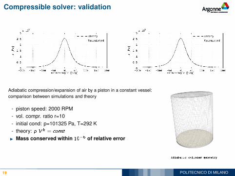
Compressible solver: validation
Adiabatic compression/expansion of air by a piston in a constant vessel:
comparison between simulations and theory
- piston speed: 2000 RPM
- vol. compr. ratio r=10
- initial cond: p=101325 Pa, T=292 K
- theory: p V
k = onst
◮ Mass conserved within 10
−5 of relative error
19
Adiabati ylinder geometry
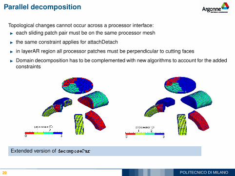
Parallel decomposition
Topological changes cannot occur across a processor interface:
◮ each sliding patch pair must be on the same processor mesh
◮ the same constraint applies for attachDetach
◮ in layerAR region all processor patches must be perpendicular to cutting faces
◮ Domain decomposition has to be complemented with new algorithms to account for the addedconstraints
Extended version of de omposePar
20
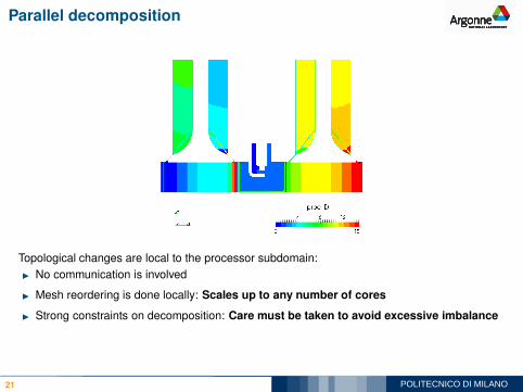
Parallel decomposition
Topological changes are local to the processor subdomain:
◮ No communication is involved
◮ Mesh reordering is done locally: Scales up to any number of cores
◮ Strong constraints on decomposition: Care must be taken to avoid excessive imbalance
21
Parallel decomposition
singlePro essorFa eSets
(
(sliding-exhValveA 1)
(sliding-exhValveB 1)
(sliding-inValveA 2)
(sliding-inValveB 2)
(exhValve-deta hFa es -1)
(inValve-deta hFa es -1)
);
layerARde omp
{
ylinderCells
{
fa eSet pistonFa es;
}
}
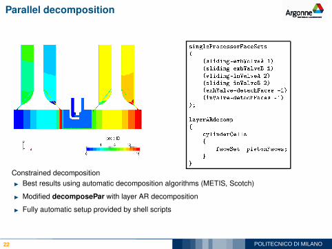
Constrained decomposition
◮ Best results using automatic decomposition algorithms (METIS, Scotch)
◮ Modified decomposePar with layer AR decomposition
◮ Fully automatic setup provided by shell scripts
22
Reconstruction for Topological Changes
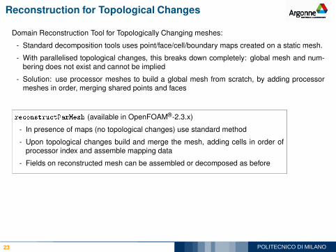
Domain Reconstruction Tool for Topologically Changing meshes:
- Standard decomposition tools uses point/face/cell/boundary maps created on a static mesh.
- With parallelised topological changes, this breaks down completely: global mesh and num-bering does not exist and cannot be implied
- Solution: use processor meshes to build a global mesh from scratch, by adding processormeshes in order, merging shared points and faces
re onstru tParMesh (available in OpenFOAM®-2.3.x)
- In presence of maps (no topological changes) use standard method
- Upon topological changes build and merge the mesh, adding cells in order ofprocessor index and assemble mapping data
- Fields on reconstructed mesh can be assembled or decomposed as before
23
Turbulence modeling: DLRM
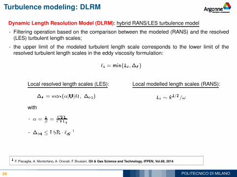
Dynamic Length Resolution Model (DLRM): hybrid RANS/LES turbulence model
- Filtering operation based on the comparison between the modeled (RANS) and the resolved(LES) turbulent length scales;
- the upper limit of the modeled turbulent length scale corresponds to the lower limit of theresolved turbulent length scales in the eddy viscosity formulation:
ℓt
= min{Lt
,∆f
}
Local resolved length scales (LES):
∆f
= max(α|U|δt, ∆eq
)
with
- α = 1
β= CFL
CFL
i
- ∆eq
≤ LSR · ℓdi
1
Local modelled length scales (RANS):
L
t
∼ k
1/2/ω
24
1
F. Piscaglia, A. Montorfano, A. Onorati, F. Brusiani. Oil & Gas Science and Technology, IFPEN, Vol.69, 2014
Turbulence modeling: DLRM
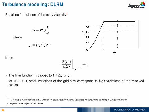
Resulting formulation of the eddy viscosity1
µt
= g
2 ρk
ω
where
g ≡ (ℓt
/Lt
)2/3
Note:∂(
g
2
)
∂∆f
∣
∣
∣
∣
∣
∆f
→0
→ 0
- The filter function is clipped to 1 if ∆f
> L
t
.
- for ∆f
→ 0, small variations of the grid size correspond to high variations of the resolvedscales
25
1
F. Piscaglia, A. Montorfano and A. Onorati. “A Scale Adaptive Filtering Technique for Turbulence Modeling of Unsteady Flows in
IC Engines”. SAE paper 2015-01-0395
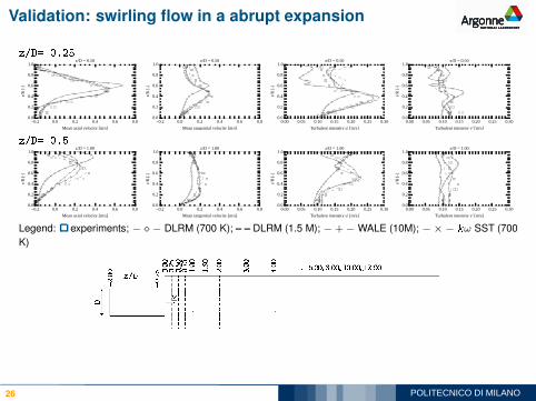
Validation: swirling flow in a abrupt expansion
z/D= 0.25
−0.2 0.0 0.2 0.4 0.6 0.8Mean axial velocity [m/s]
0.0
0.2
0.4
0.6
0.8
1.0
r/R []
z/D = 0.50
−0.2 0.0 0.2 0.4 0.6 0.8Mean tangential velocity [m/s]
0.0
0.2
0.4
0.6
0.8
1.0
r/R []
z/D = 0.50
0.00 0.05 0.10 0.15 0.20 0.25 0.30Turbulent intensity u' [m/s]
0.0
0.2
0.4
0.6
0.8
1.0
r/R [
]
z/D = 0.50
0.00 0.05 0.10 0.15 0.20 0.25 0.30Turbulent intensity v' [m/s]
0.0
0.2
0.4
0.6
0.8
1.0
r/R [
]
z/D = 0.50
z/D= 0.5
−0.2 0.0 0.2 0.4 0.6 0.8Mean axial velocity [m/s]
0.0
0.2
0.4
0.6
0.8
1.0
r/R []
z/D = 1.00
−0.2 0.0 0.2 0.4 0.6 0.8Mean tangential velocity [m/s]
0.0
0.2
0.4
0.6
0.8
1.0r/R
[]
z/D = 1.00
0.00 0.05 0.10 0.15 0.20 0.25 0.30Turbulent intensity u' [m/s]
0.0
0.2
0.4
0.6
0.8
1.0
r/R [
]
z/D = 1.00
0.00 0.05 0.10 0.15 0.20 0.25 0.30Turbulent intensity v' [m/s]
0.0
0.2
0.4
0.6
0.8
1.0
r/R [
]
z/D = 1.00
Legend: experiments; − ⋄− DLRM (700 K); – – DLRM (1.5 M); −+− WALE (10M); −×− kω SST (700
K)
26
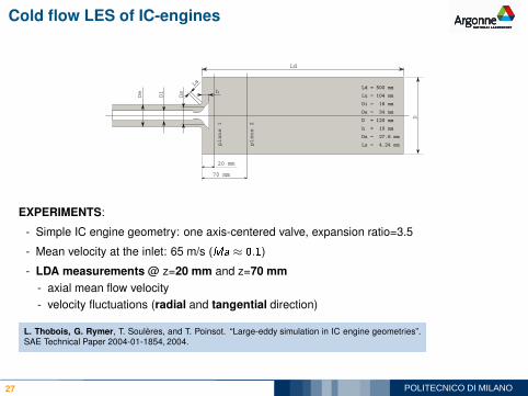
Cold flow LES of IC-engines
20 mm
70 mm
plane 1
plane 2
Ld = 500 mm
Lu = 104 mm
Di = 16 mm
De = 34 mm
D = 120 mm
h = 10 mm
Ds = 27.6 mm
Ls = 4.24 mm
Ld
D
De
Di
Ds
Ls
h
EXPERIMENTS:
- Simple IC engine geometry: one axis-centered valve, expansion ratio=3.5
- Mean velocity at the inlet: 65 m/s (Ma ≈ 0.1)
- LDA measurements @ z=20 mm and z=70 mm
- axial mean flow velocity
- velocity fluctuations (radial and tangential direction)
L. Thobois, G. Rymer, T. Soulères, and T. Poinsot. “Large-eddy simulation in IC engine geometries”.SAE Technical Paper 2004-01-1854, 2004.
27
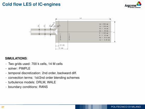
Cold flow LES of IC-engines
20 mm
70 mm
plane 1
plane 2
Ld = 500 mm
Lu = 104 mm
Di = 16 mm
De = 34 mm
D = 120 mm
h = 10 mm
Ds = 27.6 mm
Ls = 4.24 mm
Ld
D
De
Di
Ds
Ls
h
SIMULATIONS:
- Two grids used: 700 k cells, 14 M cells
- solver: PIMPLE
- temporal discretization: 2nd order, backward diff.
- convection terms: 1st/2nd order blending schemes
- turbulence models: DRLM, WALE
- boundary conditions: RANS
27
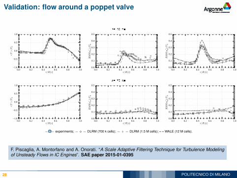
Validation: flow around a poppet valve
z= 20 mm
0.0 0.2 0.4 0.6 0.8 1.0r/R []
−1.0
−0.5
0.0
0.5
1.0
<U>/U
0
0.0 0.2 0.4 0.6 0.8 1.0r/R []
0.0
0.1
0.2
0.3
0.4
0.5
RMS(u
′ ax)/U
0
0.0 0.2 0.4 0.6 0.8 1.0r/R []
0.0
0.1
0.2
0.3
0.4
0.5
RMS(u
′ tg)/U
0
z= 70 mm
0.0 0.2 0.4 0.6 0.8 1.0r/R []
−1.0
−0.5
0.0
0.5
1.0
<U>/U
0
0.0 0.2 0.4 0.6 0.8 1.0r/R []
0.0
0.1
0.2
0.3
0.4
0.5
RMS(u
′ ax)/U
0
0.0 0.2 0.4 0.6 0.8 1.0r/R []
0.0
0.1
0.2
0.3
0.4
0.5
RMS(u
′ tg)/U
0
− − experiments; − ⋄ − DLRM (700 k cells); − + − DLRM (1.5 M cells); – – WALE (12 M cells).
F. Piscaglia, A. Montorfano and A. Onorati. “A Scale Adaptive Filtering Technique for Turbulence Modelingof Unsteady Flows in IC Engines”. SAE paper 2015-01-0395
28
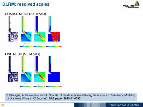
DLRM: resolved scales
COARSE MESH (700 k cells)
FINE MESH (5.3 M cells)
F. Piscaglia, A. Montorfano and A. Onorati. “A Scale Adaptive Filtering Technique for Turbulence Modelingof Unsteady Flows in IC Engines”. SAE paper 2015-01-0395
29
DLRM: features
ADVANTAGES
- General formulation of the filtering operation: filtering can be applied to any turbulence model(k-ω-SST is used in the examples)
- Grid size is the control parameter to automatically switch from RANS to LES;
- Smooth transition from RANS to LES thanks to the filter function g
2;
- Easy set-up: “RANS-type” boundary conditions
- Time resolved turbulence model
DRAWBACKS
- LES post-processing (averaging..)
F. Piscaglia, A. Montorfano and A. Onorati. “A Scale Adaptive Filtering Technique for Turbulence Modelingof Unsteady Flows in IC Engines”. SAE paper 2015-01-0395
30
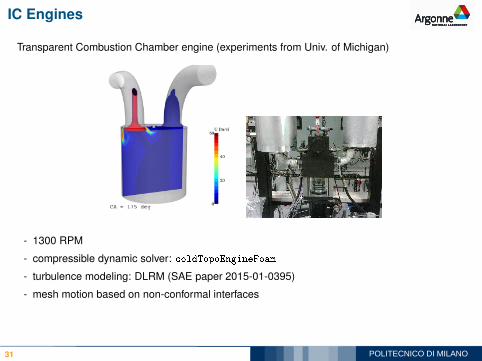
IC Engines
Transparent Combustion Chamber engine (experiments from Univ. of Michigan)
- 1300 RPM
- compressible dynamic solver: oldTopoEngineFoam
- turbulence modeling: DLRM (SAE paper 2015-01-0395)
- mesh motion based on non-conformal interfaces
31
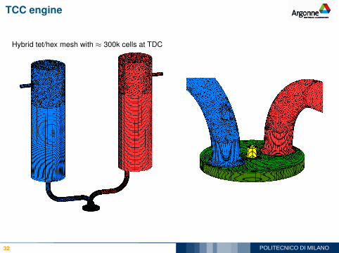
TCC engine
Hybrid tet/hex mesh with ≈ 300k cells at TDC
32
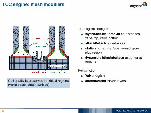
TCC engine: mesh modifiers
Cell quality is preserved in critical regions(valve seats, piston surface)
Topological changes
◮ layerAdditionRemoval on piston top,valve top, valve bottom
◮ attachDetach on valve seat
◮ static slidingInterface around sparkplug region
◮ dynamic slidingInterface under valveregions
Point motion
◮ Valve region
◮ attachDetach Piston layers
33
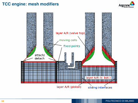
TCC engine: mesh modifiers
34
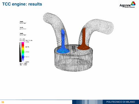
TCC engine: results
35
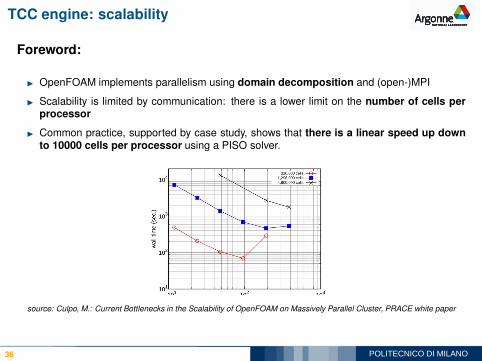
TCC engine: scalability
Foreword:
◮ OpenFOAM implements parallelism using domain decomposition and (open-)MPI
◮ Scalability is limited by communication: there is a lower limit on the number of cells perprocessor
◮ Common practice, supported by case study, shows that there is a linear speed up downto 10000 cells per processor using a PISO solver.
source: Culpo, M.: Current Bottlenecks in the Scalability of OpenFOAM on Massively Parallel Cluster, PRACE white paper
36
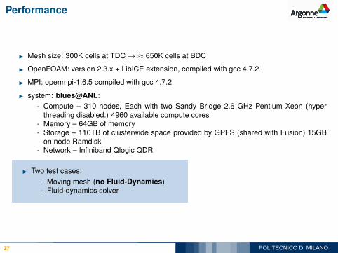
Performance
◮ Mesh size: 300K cells at TDC → ≈ 650K cells at BDC
◮ OpenFOAM: version 2.3.x + LibICE extension, compiled with gcc 4.7.2
◮ MPI: openmpi-1.6.5 compiled with gcc 4.7.2
◮ system: blues@ANL:
- Compute – 310 nodes, Each with two Sandy Bridge 2.6 GHz Pentium Xeon (hyperthreading disabled.) 4960 available compute cores
- Memory – 64GB of memory- Storage – 110TB of clusterwide space provided by GPFS (shared with Fusion) 15GB
on node Ramdisk- Network – Infiniband Qlogic QDR
◮ Two test cases:
- Moving mesh (no Fluid-Dynamics)- Fluid-dynamics solver
37
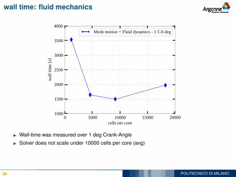
wall time: fluid mechanics
0 5000 10000 15000 20000cells per core
1000
1500
2000
2500
3000
3500
4000
wall tim
e [s]
Mesh motion + Fluid dynamics 1 CA deg
◮ Wall-time was measured over 1 deg Crank-Angle
◮ Solver does not scale under 10000 cells per core (avg)
38
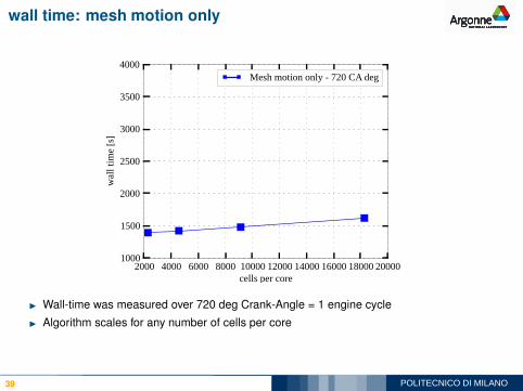
wall time: mesh motion only
2000 4000 6000 8000 10000 12000 14000 16000 18000 20000cells per core
1000
1500
2000
2500
3000
3500
4000
wall tim
e [s]
Mesh motion only 720 CA deg
◮ Wall-time was measured over 720 deg Crank-Angle = 1 engine cycle
◮ Algorithm scales for any number of cells per core
39
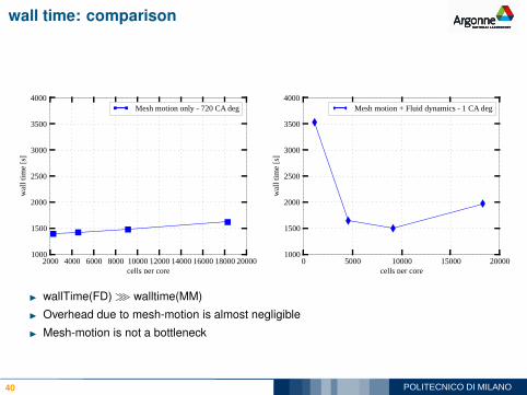
wall time: comparison
2000 4000 6000 8000 10000 12000 14000 16000 18000 20000cells per core
1000
1500
2000
2500
3000
3500
4000
wall tim
e [s]
Mesh motion only 720 CA deg
0 5000 10000 15000 20000cells per core
1000
1500
2000
2500
3000
3500
4000
wall tim
e [s]
Mesh motion + Fluid dynamics 1 CA deg
◮ wallTime(FD) ≫ walltime(MM)
◮ Overhead due to mesh-motion is almost negligible
◮ Mesh-motion is not a bottleneck
40
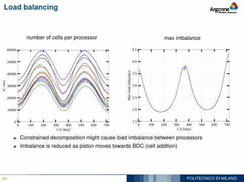
Load balancing
number of cells per processor
0 100 200 300 400 500 600 700CA [deg]
0
10000
20000
30000
40000
50000
60000
N. c
ells
max imbalance
0 100 200 300 400 500 600 700CA [deg]
1.5
2.0
2.5
3.0
3.5
4.0
4.5
Max lo
ad im
balance
◮ Constrained decomposition might cause load imbalance between processors
◮ Imbalance is reduced as piston moves towards BDC (cell addition)
41
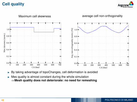
Cell quality
Maximum cell skewness
0 100 200 300 400 500 600 700CA [deg]
0.0
0.2
0.4
0.6
0.8
1.0
Max sk
ewness (n
orm.)
average cell non-orthogonality
0 100 200 300 400 500 600 700CA [deg]
0.0
0.2
0.4
0.6
0.8
1.0
Avg. nonorth
ogonality
(norm.) [%
]◮ By taking advantage of topoChanges, cell deformation is avoided
◮ Mes quality is almost constant during the whole simulation⇒Mesh quality does not deteriorate: no need for remeshing
42
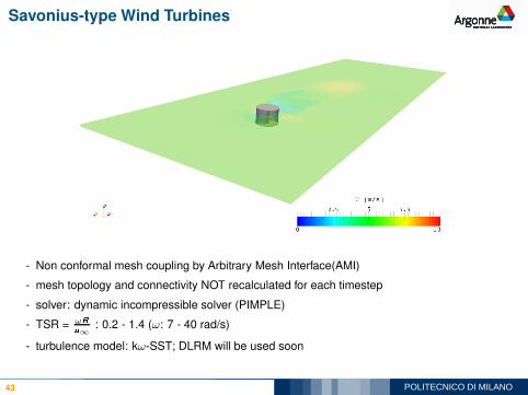
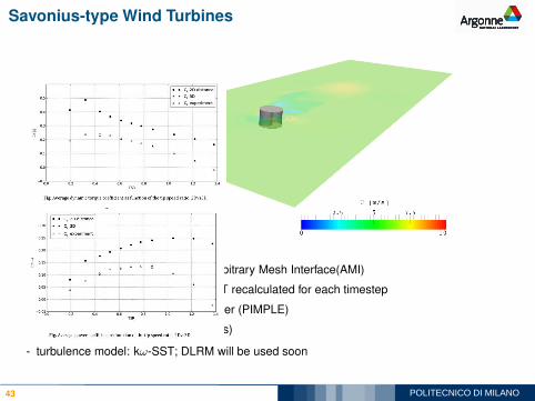
Savonius-type Wind Turbines
- Non conformal mesh coupling by Arbitrary Mesh Interface(AMI)
- mesh topology and connectivity NOT recalculated for each timestep
- solver: dynamic incompressible solver (PIMPLE)
- TSR = ωR
u∞
: 0.2 - 1.4 (ω: 7 - 40 rad/s)
- turbulence model: kω-SST; DLRM will be used soon
43
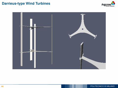
Darrieus-type Wind Turbines
44
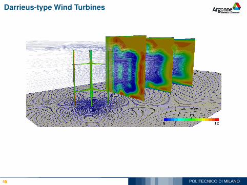
Darrieus-type Wind Turbines
45
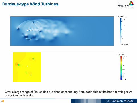
Darrieus-type Wind Turbines
Over a large range of Re, eddies are shed continuously from each side of the body, forming rowsof vortices in its wake.
46
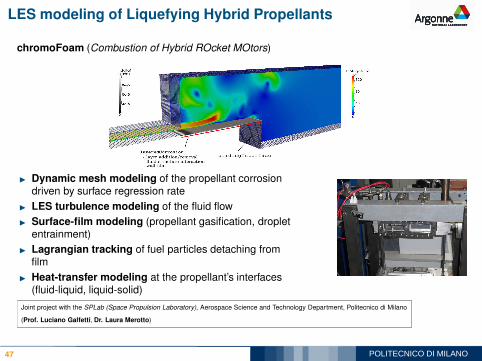
LES modeling of Liquefying Hybrid Propellants
chromoFoam (Combustion of Hybrid ROcket MOtors)
◮ Dynamic mesh modeling of the propellant corrosiondriven by surface regression rate
◮ LES turbulence modeling of the fluid flow
◮ Surface-film modeling (propellant gasification, dropletentrainment)
◮ Lagrangian tracking of fuel particles detaching fromfilm
◮ Heat-transfer modeling at the propellant’s interfaces(fluid-liquid, liquid-solid)
Joint project with the SPLab (Space Propulsion Laboratory), Aerospace Science and Technology Department, Politecnico di Milano
(Prof. Luciano Galfetti, Dr. Laura Merotto)
47
Conclusions
Extension of mesh motion features for ICE in OpenFOAM-2.3.x:
- automatic motion solver for IC engines
- layer addition/removal
- algorithm to couple/decouple of non-conformal mesh regions
- improved compressible solver
- decomposition algorithms
Example of application: TCC engine
- Simulation of a whole engine cycle with a single mesh
- Cell quality preserved during the entire simulation
Numerical performance
- Scalable mesh motion algorithm
- Mesh motion overhead negligible w.r.t fluid-dynamics solver
- To improve: constrained decomposition can lead to unbalanced domains
48
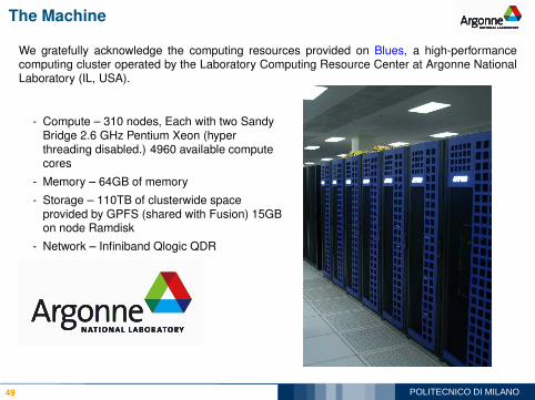
The Machine
We gratefully acknowledge the computing resources provided on Blues, a high-performancecomputing cluster operated by the Laboratory Computing Resource Center at Argonne NationalLaboratory (IL, USA).
- Compute – 310 nodes, Each with two SandyBridge 2.6 GHz Pentium Xeon (hyperthreading disabled.) 4960 available computecores
- Memory – 64GB of memory
- Storage – 110TB of clusterwide spaceprovided by GPFS (shared with Fusion) 15GBon node Ramdisk
- Network – Infiniband Qlogic QDR
49
Thank you for your attention!
50
Andrea Montorfano, Ph.D.Post-doc Researcher
CONTACT INFORMATION
Address Dipartimento di Energia, Politecnico di Milano
via Lambruschini 4, 20156 Milano (ITALY)
E-Mail: [email protected]
Phone: (+39) 02 2399 3804
Web page: http://www.engines.polimi.it/
51
References I
1. A. Montorfano, F. Piscaglia, and A Onorati. An Extension of the Dynamic Mesh Handling with Topological Changes for LES of ICE in OpenFOAM.
SAE paper 2015-01-0384, 2015. SAE World Congress & Exhibition, Detroit, Michigan (USA).
2. F. Piscaglia, A. Montorfano, and A. Onorati. A Scale Adaptive Filtering Technique for Turbulence Modeling of Unsteady Flows in IC Engines. SAE Int.
J. Engines, Paper n. 2015-01-0395, 2015.
3. F. Piscaglia, A. Montorfano, and A. Onorati. Adaptive LES of dynamically changing geometries in OpenFOAM®: an application to the TCC test case.
In LES4ICE - LES for Internal Combustion Engine Flows@IFPEN, Rueil-Malmaison, 4-5 December, 2014.
4. F. Piscaglia, A. Montorfano, and A. Onorati. Towards the les simulation of ic engines with parallel topologically changing meshes. SAE TechnicalPaper 2013-01-1096, 2013.
5. A. Montorfano, F. Piscaglia, and A. Onorati. Wall-adapting subgrid-scale models to apply to large eddy simulation of internal combustion engines.
International Journal of Computer Mathematics, in Press, 2013.
6. F. Piscaglia, A. Montorfano, A. Onorati, and F. Brusiani. Boundary conditions and subgrid scale models for les simulation of ic engines. in
proceedings of “Oil & Gas Science and Technology”, 2013.
7. F. Piscaglia, A. Montorfano, A. Onorati, and J. P. Keskinen. Boundary conditions and subgrid scale models for les simulation of internal combustion
engines. In International Multidimensional Engine Modeling User’s Group Meeting 2012, Detroit, 2012.
8. F. Piscaglia, A. Montorfano, and A. Onorati. Development of a non-reflecting boundary condition for multidimensional nonlinear duct acoustic
computation. Journal of Sound and Vibration, 332(4):922 – 935, 2013.
9. A. Montorfano, F. Piscaglia, and G. Ferrari. Inlet boundary conditions for incompressible les: A comparative study. Mathematical and Computer
Modelling, 2011.
10. F. Piscaglia, A. Montorfano, G. Ferrari, and G. Montenegro. High resolution central schemes for multi-dimensional non-linear acoustic simulation of
silencers in internal combustion engines. Mathematical and Computer Modelling, 54(7-8):1720–1724, 2011.
11. A. Onorati, G. D’Errico, T. Lucchini, G. Montenegro, and F. Piscaglia. Development of a multi-dimensional tool for the simulation of the combustion
and in-cylinder flows using the openfoam technology. In 11th Stuttgart International Symposium on Automotive and Engine Technology, Stuttgart,
2011.
12. F. Piscaglia, A. Montorfano, and A. Onorati. Development of nscbc for compressible navier-stokes equations in openfoam. In Sixth OpenFOAM
Workshop, Penn State, June 12th-16th, 2011.
13. F. Piscaglia, A. Montorfano, and A. Onorati. Multi-dimensional computation of compressible reacting flows through porous media to apply to internalcombustion engine simulation. Mathematical and Computer Modelling, 52(7-8):1133 – 1142, 2010.
52
References II
14. F. Piscaglia, A. Montorfano, A. Onorati, and G. Ferrari. Modeling of pressure wave reflection from open-ends in i.c.e. duct systems. SAE Technical
Paper 2010-01-1051, 2010.
15. G. Montenegro, F. Piscaglia, A. Montorfano, and A. Onorati. Multi-dimensional parallel simulation of diesel exhaust after-treatment systems. In
International Multidimensional Engine Modeling User’s Group Meeting 2010, Detroit, 2010.
16. F. Piscaglia, A. Montorfano, G. Montenegro, A. Onorati, H. Jasak, and H. Rusche. Lib-ice: a c++ object oriented library for ice simulation - acoustics
and aftertreatment. In Fifth OpenFOAM Workshop, Goteborg, June 21-24, 2010., 2011.
17. F. Piscaglia and G. Ferrari. A novel 1d approach for the simulation of unsteady reacting flows in diesel exhaust after-treatment systems. Energy,34(12):2051–2062, 2009.
18. F. Piscaglia and G. Ferrari. “Development of an offline simulation tool to test the on-board diagnostic software for diesel after-treatment systems”.SAE paper n. 2007-01-0133, 2007.
19. F. Piscaglia Montenegro G, A. Onorati. Impact of ultra low thermal inertia manifolds on emission performance. Atti del 62°Congresso Nazionale ATI,
Salerno, 2007.
20. G. Montenegro, F. Piscaglia, A. Onorati, G. Catalano, and P. Cioffi. A 1-d unsteady thermo-fluid dynamic approach for the simulation of the
hydrodynamics of diesel particulate filters. In SAE Int. Journal Of Fuels & Lubricants. SAE Technical Paper 2006-01-0262, V115-4(1), 2007.
21. F. Piscaglia and G. Ferrari. Modeling of the unsteady reacting flows in the diesel exhaust aftertreatment systems. In: ECOS 2007 Conference:
Efficiency, Cost, Optimization, Simulation and Environmental Impact of Energy . Padova, Italy, 2007.
22. G. Montenegro, G. D’Errico, A. Onorati, and F. Piscaglia. Integrated 1d-multid fluid dynamic models for the simulation of i.c.e. intake and exhaust
systems. SAE paper n. 2007-01-0495, 2007.
23. G. Montenegro, A. Onorati, and F. Piscaglia. A 1d unsteady thermo-fluid dynamic approach for the simulation of diesel particulate filters. THIESEL
2006 Int. Conference. Valencia (Spain), p. 139-162, 2006. ISBN: 84-9705-982-4.
24. F. Piscaglia, C. J. Rutland, and D. E. Foster. Development of a CFD model to study the hydrodynamic characteristics and the soot deposition
mechanism on the porous wall of a diesel particulate filter. SAE paper n. 2005-01-0963, SAE 2005 Int. Congress & Exp. (Detroit, Michigan), April
11-14, 2005.
25. F Piscaglia and A. Onorati. A computational investigation of the hydrodynamics and the soot deposition mechanism on the channel walls of a dieselparticulate filter. 60°Congresso Nazionale ATI. Roma, Italy., 2005.
26. G. Montenegro, A. Onorati, and F. Piscaglia. Integrated 1d-multid fluid dynamic models for the simulation of internal combustion engines. HTCES
2006, 12°Convegno Internazionale “Automobili e motori Hi-Tech”, Modena, 2006.
53
References III
27. D. Cacciatore, M. Ceccarani, Onorati A., and F. Piscaglia. 1d fluid dynamic modeling of multi-pipe junctions in the exhaust system of a v12
lamborghini s.i. engine. In In: HTCES 2004 - 10°Convegno Int. “Automobili e Motori Hi-Tech”, Modena, 2004.
28. G. Ferrari, A. Onorati, F. Piscaglia, and L. Spaggiari. 1d fluid dynamic modeling of secondary air injection in the exhaust aftertreatment system of s.i.
engines. In In: HTCES 2003 - 9°Convegno Internazionale “Automobili e Motori Hi-Tech”. Modena, 29-30 maggio, 2003.
29. G. Ferrari, A. Onorati, and F. Piscaglia. Fluid dynamic simulation of a six-cylinder s.i. engine with secondary air injection in the exhaust
after-treatment system. ICE 2003- SAE International Conference on Internal Combustion Engines. Capri, Italy, 2003.
54