Regional Model Simulations of Marine Boundary Layer Clouds over the

Southeast Pacific off South America. Part I: Control Experiment

Yuqing Wang∗, Shang-Ping Xie+, Haiming Xu, and Bin Wang+

International Pacific Research Center, School of Ocean and Earth Science and Technology,

University of Hawaii at Manoa, Honolulu, HI 96822

July 21, 2003

Dateline

Accepted by Monthly Weather Review

∗ Corresponding author address: Dr. Yuqing Wang, IPRC/SOEST, University of Hawaii at Manoa, 2525 Correa Road, Honolulu, HI 96822. Email: yqwang@soest.hawaii.edu + Also at Department of Meteorology, University of Hawaii, Honolulu, Hawaii.

ABSTRACT

A regional climate model is used to simulate boundary-layer stratocumulus (Sc) clouds

over the Southeast Pacific off South America during August-October 1999 and to study their

dynamical, radiative, and microphysical properties and their interaction with large-scale

dynamic fields. Part I evaluates the model performance against satellite observations and

examine physical processes important for maintaining the temperature inversion and Sc clouds

in the simulation.

The model captures major features of the marine boundary layer in the region, including

a well-mixed marine boundary layer, a capping temperature inversion, Sc clouds, and the

diurnal cycle. Sc clouds develop in the lower half of and below the temperature inversion layer

that increases its height westward off the Pacific coast of South America. The strength of the

capping inversion is determined not only by large-scale subsidence and local sea surface

temperature (SST), but also by cloud-radiation feedback. A heat budget analysis indicates that

upward longwave radiation cools strongly the upper part of the cloud layer and strengthens the

temperature inversion. This cloud-top cooling further induces a local enhancement of

subsidence in and below the inversion layer, resulting a dynamical warming that strengthens

the temperature stratification above the clouds.

While of secondary importance on the mean, solar radiation drives a pronounced

diurnal cycle in the model boundary layer. Consistent with observations, boundary-layer clouds

thicken after the sunset and cloud liquid water content reaches a maximum at 6 am of local

time just before the sunrise.

1. Introduction

Clouds reflect solar radiation, absorb (emit) longwave radiation from the earth surface

(at the cloud top) and thus play an important role in climate over a wide range of space and

time scales. Globally, cloud reflectivity increases the earth’s albedo with a net effect to cool

the earth climate system (Hartmann et al. 1992). A main contribution to the cloud albedo effect

comes from marine boundary layer clouds, which cover on average 34% of the ocean surface

(Klein and Hartmann 1993, Norris 1998). The high albedo (30-40%) of the marine boundary

layer (MBL) stratocumulus/stratus clouds compared to the ocean background (~ 8%) gives rise

to large deficits in the absorbed solar radiative fluxes both at the top of the atmosphere and at

the ocean surface, while their low altitudes prevent significant compensation by thermal

emission (Randall et al. 1984). Thus, boundary layer clouds cool both the atmosphere and the

ocean below in general. They are also important for the thermal and moisture structures of the

MBL and the fluxes both at the sea surface and across the temperature inversion, through

condensation and precipitation, turbulence generation, and radiative transfer (Yuter et al. 2000;

Garreaud et al. 2001; McCaa and Bretherton 2003). In addition to these local effects, the cloud-

top longwave radiation cools the MBL, leading to a large-scale adjustment in dynamical fields

(Nigam 1997; Bergman and Hendon 2000).

There exists an extensive stratocumulus (Sc) cloud deck over the Southeast Pacific off

South America due to mainly the large-scale subsidence in the subtropical ocean and the

coastal upwelling-induced cold sea surface temperature (SST), both favoring the formation of a

low-level temperature inversion and boundary layer clouds. The cloud deck shields incoming

solar radiation and cools the ocean, while the sea surface cooling in turn helps maintain the Sc

clouds. This positive feedback and its effect on the meridional configuration of the intertropical

convergence zone (ITCZ) over the eastern Pacific have been demonstrated by Ma et al. (1996)

1

and Philander et al. (1996) with coupled general circulation model (GCM) experiments. In their

experiments, the radiative cooling due to the prescribed/parameterized boundary layer clouds in

the southeastern equatorial Pacific cools the local SST and increases SST gradients in both the

meridional and zonal directions, strengthening the southeasterly trade winds and leading to

basin-wide adjustments in the ocean and atmosphere (Yu and Mechoso 1999; Gordon et al.

2000), through their mutual interaction (Xie et al. 1996).

Despite their climatic importance, MBL Sc clouds are poorly represented in most of the

global atmospheric GCMs (Delecluse et al. 1998) because of insufficient model resolution

and/or inadequate physical parameterizations. This deficiency in simulating boundary layer

clouds appears to be responsible for the failure of many coupled GCMs to keep the ITCZ north

of the equator and maintain an equatorial cold tongue of adequate strength over the eastern

Pacific (Mechoso et al. 1995; Frey et al. 1997; Delecluse et al. 1998). Recently several groups

have reported improved simulation of Sc clouds in GCMs. Bachiochi and Krishnamurti (2000)

develop an empirical boundary-layer cloud parameterization scheme based on the boundary

layer height, ground wetness, and the relative humidity. Teixeira and Hogan (2002) develop a

new parameterization scheme for subtropical boundary layer clouds partially based on large

eddy simulation (LES) results. These new schemes remain to be tested in other GCMs for their

robustness. This latter parameterization scheme, however, has been recently shown by

Siebesma et al. (2003) that it might overestimate the boundary layer cloud cover significantly.

The extreme opposite to global GCMs is large-eddy simulations (LESs), which have

long been used to study Sc clouds and their interaction with radiation but with crude cloud

microphysics (e.g., Deardorff 1980; Kogan et al. 1995; Krueger et al. 1995; Wyant et al. 1997;

Moeng 2000; and among others). While affording high resolution, LES models usually cover a

small area (much less than the size of a grid box of current GCMs). In these models the large-

2

scale flow fields including vertical motion must be prescribed. In reality, the interaction of Sc

clouds with large-scale fields is generally important in determining the MBL structure, as will

be shown in this study.

Regional atmospheric models are a useful bridge between global GCMs on one hand

and LES models on the other. With a limited domain, regional models can afford higher

resolution than global GCMs while still allowing interaction of MBL physics with large-scale

fields resolved. With such a regional model, McCaa and Bretherton (2003) simulate the Sc

cloud decks in the Northeast and Southeast Pacific domains separately and find that the

simulations are sensitive to the treatment of shallow cumulus convection. Since the scale for

physical-dynamical interaction is limited by the model domain size, it is generally important to

configure the domain large enough to include interactive phenomena of interest.

The present study uses a newly developed regional climate model to simulate eastern

Pacific climate in general and cloud-topped MBL in particular. Its objectives are twofold: to

demonstrate the capability of the model in simulating the Sc clouds over the Southeast Pacific

off South America; and to investigate the physical processes that maintain the temperature

inversion and clouds. We use a much larger model domain than that in McCaa and Bretherton

(2003) to cover not only the Southeast but also the Northeast Pacific Oceans so that interaction

between the northward-displaced ITCZ and Sc cloud deck can be studied. Part II of this series

will report on sensitivity experiments that explore this interaction.

Recent satellite microwave observations offer a view of the ocean and overlying

atmosphere at unprecedented resolution and coverage (Wentz et al. 2000; Xie et al. 2001). For

model validation, we take advantage of these new measurements, specifically those of column

cloud liquid water and precipitation by the Tropical Rain Measuring Mission (TRMM) satellite

(Wentz et al. 2000), and those of surface wind velocity by the QuikSCAT satellite (Liu et al.

3

2000; Chelton et al. 2001). The TRMM and QuikSCAT datasets are both available at 0.25o H

0.25o and daily resolution. In particular, column cloud liquid water represents a test of models

more stringent than traditional cloud fraction observed by visible and infrared sensors.

The rest of the paper is organized as follows. Section 2 briefly describes the regional

climate model used. Section 3 presents the simulation results, including the large-scale

circulation, boundary layer structure, clouds, and the cloud radiative forcing. Section 4

examines the mechanisms for maintaining the temperature inversion and cloud layers through a

heat budget analysis. Section 5 presents an analysis of diurnal cycle of the cloud-capped MBL

in the model. Section 6 gives main conclusions and discusses the major deficiencies in the

current simulation.

2. Model description and experimental design

a. IPRC–RegCM model

The numerical model used in this study is the regional climate model recently

developed at the International Pacific Research Center (hereafter IPRC–RegCM). A detailed

description of the IPRC–RegCM and its performance in simulating regional climate over East

Asia can be found in Wang et al. (2003). This model was developed based on a high-resolution

tropical cyclone model previously developed by Wang (2001, 2002). Some key features of the

model critical to the simulation in this study are highlighted here.

The model uses hydrostatic primitive equations in spherical coordinates in the

horizontal and in F (pressure normalized by surface pressure) coordinate in the vertical. It is

solved numerically with a fourth-order conservative finite-difference scheme on an unstaggered

longitude/latitude grid system and a second-order leapfrog scheme with intermittent use of

Euler backward scheme for time integration. The model has 28 vertical levels with substantial

4

concentration of resolution within the planetary boundary layer (10 levels below 800 hPa). The

model physics are carefully chosen based on the up-to-date developments.

The cloud microphysics scheme developed by Wang (2001) is used to represent the grid

resolved moist processes. Prognostic variables are mixing ratios of water vapor, cloud water,

rainwater, cloud ice, snow, and graupel. Subgrid shallow convection, midlevel convection, and

penetrative deep convection are parameterized based on the mass flux scheme originally

developed by Tiedtke (1989), and later modified by Gregory et al. (2000). This modified

version uses a CAPE (convective available potential energy) closure instead of the previous

moisture convergence closure and considers the organized entrainment and detrainment based

on a simple cloud plume model. The detrained cloud water/ice at the top of cumulus towers are

added to the grid-scale values (Wang et al. 2003) but modified to be dependent on the

environmental relative humidity so that immediate evaporation of detrained clouds is allowed

for dry conditions. For realistic simulation of the boundary layer clouds, we have adjusted the

fraction of the cloud ensemble that penetrates into the inversion layer and detrains there into the

environment from default value 0.33 to 0.23 for shallow convection. As indicated by Tiedtke

(1989), the original value was determined based on some sensitivity experiments using a single

column model. Our sensitivity experiments showed that the large value may produce much less

boundary layer clouds due to the fact that too much cloud water would be detrained across the

inversion and evaporates there, in agreement with the results of Tiedtke (1989).

The subgrid scale vertical mixing is accomplished by the so-called E-, turbulence

closure scheme in which both turbulent kinetic energy and its dissipation rate are prognostic

variables (Detering and Etling 1985). In our application, we include both advection and the

effect of moist-adiabatic processes in cloudy air on the buoyancy production of turbulence

(Durran and Klemp 1982). Turbulent fluxes at the ocean surface are calculated using the

5

modified Monin-Obukhov scheme (Wang 2002). Turbulent fluxes over the land surface are

calculated based on the bulk aerodynamic method used in the land surface module, which uses

the Biosphere-Atmosphere Transfer Scheme (BATS) developed by Dickinson et al. (1993).

BATS incorporates one canopy and three soil layers, and it requires land cover/vegetation (18

types), soil texture (12 types) and soil color (8 types) maps for spatial applications. These are

obtained from the U.S. Geological Survey 1-km resolution land cover classification dataset and

the U.S. Department of Agriculture global 10-km soil data.

The radiation package originally developed by Edwards and Slingo (1996) and further

improved later by Sun and Rikus (1999) is used in the model. This radiation scheme includes

seven/four bands for longwave/shortwave radiation calculations. Surface albedos of diffuse and

direct radiations calculated in the land surface model are directly used in determining the

shortwave radiation budget. The cloud optical properties are calculated based on Sun and Shine

(1994) for longwave radiation, while based on Slingo and Schrecker (1982) and Chou et al.

(1998) for shortwave radiation. A recent study by Sun and Pethick (2002) indicates that the

above combination of parameterizations is suitable for MBL Sc clouds. Cloud amount is

diagnosed using the semi-empirical cloudiness parameterization scheme developed by Xu and

Randall (1996) based on the results from cloud resolving model simulations. By this scheme,

cloud amount is determined by both relative humidity and liquid/ice water content. Recently,

Siebesma et al. (2003) show that Xu and Randall’s scheme can produce quite realistic

cloudiness estimate of boundary layer clouds.

The regional atmospheric model is run with both initial and lateral boundary conditions

from either reanalysis dataset or from output from a global atmospheric model. A one-way

nesting is used to update the model time integration in a buffer zone near the lateral boundaries

within which the model prognostic variables are nudged to the reanalysis data or the global

6

model results. An inflow-outflow boundary condition is used for water vapor with a very weak

nudging in the buffer zone to prevent the moisture field from drifting away from the driving

fields. Since there are no hydrometeor fields provided by the driving fields, we simply ignored

the horizontal advection of mixing ratios of cloud water, rainwater, cloud ice, snow and graupel

at inflow boundaries, while they are advected outward at the outflow boundaries. This

inflow/outflow boundary condition is also used for both turbulent kinetic energy and its

dissipation rate.

b. Experimental design

The regional climate model described above is used to simulate the extensive Sc clouds

over the Southeast Pacific off South America in boreal fall (August–October, hereafter ASO).

In this study, the case in 1999 is chosen because it was a moderate La Nino year and because of

the availability of TRMM and QuikSCAT data for model verification. The model domain was

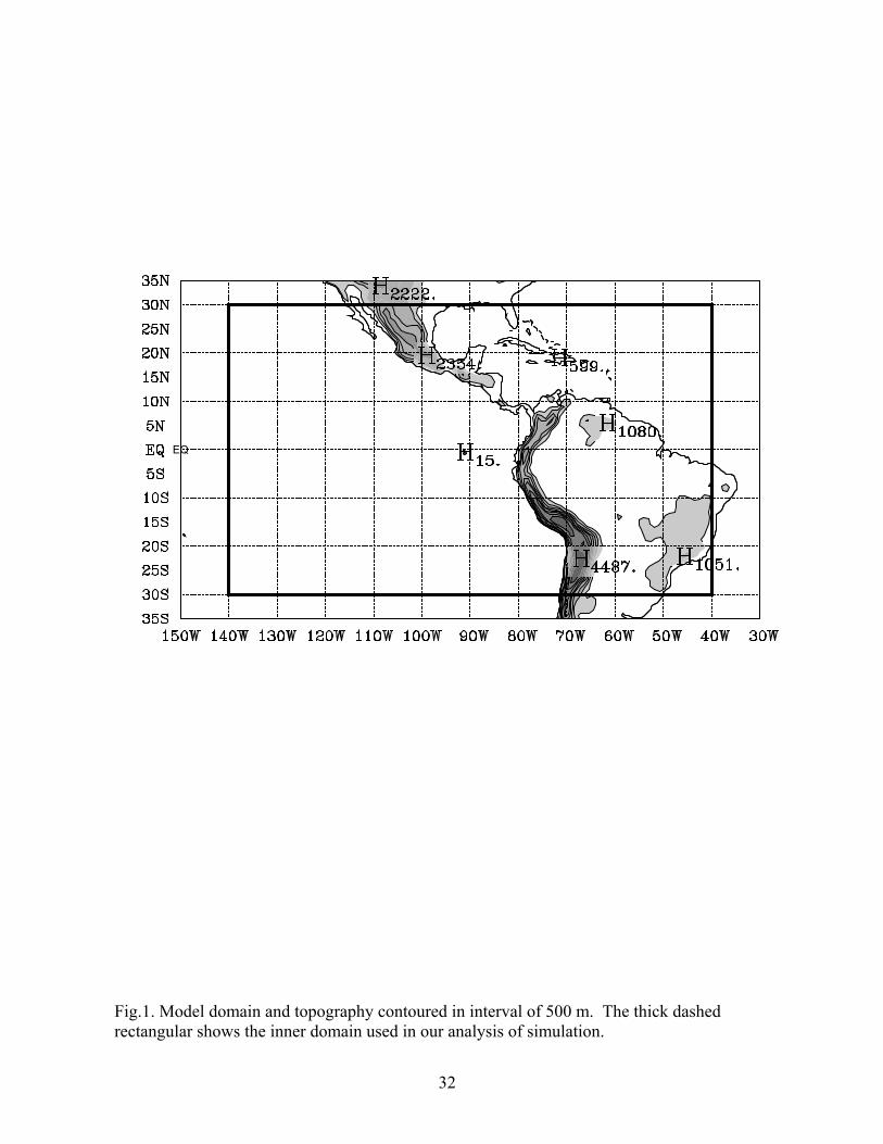
defined in the area of 35oS–35oN, 150oW–30oW with horizontal grid spacing of 0.5o (Fig. 1).

This domain includes a large portion of the eastern Pacific and the South American continent

and covers the areas of persistent marine Sc clouds off the west coast of South America and the

trade cumuli to the west (Klein and Hartmann 1993). The Northeast Pacific is included in the

computational domain in order to simulate the convective precipitation in the ITCZ north of the

equator, which may have a large-scale control on the Southeast Pacific Sc clouds through the

dynamically driven meridional Hadley circulation. To minimize the edge effects from the

lateral boundaries, verification is performed on an area of 30oS-30oN, 140oW-40oW (within the

dashed lined box in Fig. 1).

The National Center for Environmental Prediction–National Center for Atmospheric

Research (NCEP–NCAR) reanalysis data at every 6 h intervals with a resolution of 2.5o H 2.5o

7

in the horizontal and 17 pressure levels up to 10 hPa (Kalnay et al. 1996) are used to define the

driving fields, which provide both initial and lateral boundary conditions to the regional climate

model. Sea surface temperatures over the ocean are obtained from the Reynolds weekly SST

data with horizontal resolution of 1o H 1o (Reynolds and Smith 1994), which are interpolated

into the model grids by cubic spline interpolation in space and linearly interpolated in time.

Over the land, the initial surface soil and canopy temperatures are obtained from the lowest

model level with a standard lapse rate of 6.5oC/km. Initial snow depths are set to zero, while the

soil moisture fields are initialized such that the initial soil moisture depends on the vegetation

and soil types defined for each grid cell (Giorgi and Bates 1989)

The USGS high-resolution topographic dataset (0.0833o H 0.0833o) is used to obtain the

model topography. We first calculate the averaged topographic height within the model grid

box (0.5o by 0.5o) using the USGS data and then added the standard deviation to the averaged

value to get the envelope topography for this grid box (contours in Fig. 1). The high-resolution

vegetation type data from U.S. Geophysical Survey is reanalyzed for the model based on

dominant vegetation type in each grid box.

The model is initialized at 00Z on July 29 and integrated continuously through October

31, 1999. This experiment serves as our control simulation. Note that the initial three-day

integration in July is used to spin up the model physics, such as the planetary boundary layer

and cloud processes, and thus is excluded from our analysis below.

3. Simulation results

a. Large-scale circulation and precipitation

Mean conditions of the eastern Pacific climate are well simulated by the regional

climate model for ASO in 1999. In the upper troposphere (Fig. 2a), the subtropical ridge is

8

centered at about 10oS with the subtropical westerly jet located to the south and equatorial

easterlies to the north. In the lower troposphere (Fig. 2b), the subtropical anticyclone occupies

the Southeast Pacific with its center located at about 110oW, 25oS, driving large-scale

southeasterly winds over most of the Southeast Pacific. The southeasterlies accelerate on their

way toward the equator, giving rise to large-scale divergence and subsidence over the

southeastern Pacific, especially off the west coast of South America. This large-scale

circulation favors the formation of both the temperature inversion and Sc clouds there

(Garreaud et al. 2001). To the north of the equator near the west coast of Mexico (Fig. 2b) is an

east-west elongated cyclonic shear zone, where the mean ITCZ is located during the boreal fall.

Compared to TRMM observations (Fig. 3a), overall, the model simulates the seasonal

mean precipitation quite well over the Pacific and Atlantic (Fig. 3c), both in spatial distribution

and magnitude. Note that the TRMM data have a higher spatial resolution (0.25o by 0.25o) than

the model and thus give much more detailed structure of precipitation. We notice that satellite

rain measurements are still subject to quantitative uncertainties. During the same time period,

CPC Merged Analysis of Precipitation (CMAP; Xie and Arkin 1996) gives much small rain

rates than TRMM but shows a quite similar spatial pattern (Fig. 3b).

The model also simulates the light precipitation (less than 1 mm d-1), usually named

drizzle, under the SC cloud deck over the southeast Pacific (Fig. 3d). Drizzle and column cloud

liquid water (Fig. 5b) show similar patterns in the simulation. Such drizzle under boundary

layer clouds has been reported in several observational (Miller and Albrecht 1995; Garreaud et

al. 2001) and LES (e.g., Wyant et al. 1997) studies. Drizzle is an important feature of Sc

clouds, modifying the temperature and moisture structure of the MBL as they precipitate

through the unsaturated subcloud layer and undergo evaporation (see section 4).

9

The overall spatial pattern of the simulated surface winds (Fig. 4a) resembles the

QuikSCAT observations (Fig. 4b) except for slightly higher wind speeds (about 1 m s-1 higher),

especially in the equatorial cold–tongue region where the minimum SST occurs (Chelton et al.

2001). This overestimation of surface wind speed in the equatorial region may result partly

from the use of a coarse-resolution (1o x 1o) SST product with weaker gradients used in the

model (shaded colors in Fig. 3c) than the real SST. In addition, the QuikSCAT does not really

measure surface wind but the stress at the interface of moving air and water. As noticed by

Kelly et al. (2001), the deceleration of QuikSCAT winds over the equatorial Pacific might be

partly due to the effect of the westward South Equatorial Current and the eastward North

Equatorial Countercurrent.

b. Boundary layer structure and clouds

Figure 5 compares the ASO mean column cloud liquid water content between the

TRMM data (a) and the model simulation (b). The model reproduces the high cloud liquid

water content in the east-west oriented ITCZ between 5oN-15oN, except for an underestimation

off the Pacific coast north of the equator and over the Atlantic and Caribbean Sea and an

overestimation over the Pacific offshore. Over regions with little precipitation south of the

equator, the cloud water simulation compares reasonably well with TRMM observations both

in spatial distribution and magnitude except for a westward shift of the cloud deck south of the

equator. Such an unrealistic shift also appeared in McCaa and Bretherton (2003, see their Fig.

12) and might be due to the coarse model resolution that could not resolve the high steep

Andean mountain and the land-sea contrast well. The model also overestimates the cloud liquid

water content near the equatorial region west of 90oW and underestimates it in the proxy of the

10

west coast off South America. Despite these discrepancies, the model simulation of the cloud

distribution is reasonably well, unlike most current GCMs.

The model simulates very rich structures in the planetary boundary layer (PBL). Figure

6a shows a zonal-vertical cross-section along 10oS of cloud liquid water mixing ratio (shaded),

temperature (solid contours) and virtual potential temperature (thin dashed contours), together

with the d2v/dp = 8 K/100hPa (thick dashed curves) that is taken as a weak criterion for

temperature inversion layer. The PBL is very shallow with a strong temperature inversion off

the west coast of South America, consistent with Paluch et al.’s (1999) dropsonde observations.

The rapid rise of the PBL toward the west as SST increases (Fig. 6a) is well simulated. There

seem different regimes of the PBL structure and boundary layer clouds east and west of 100oW.

To the east, the well-mixed marine PBL (vertically near constant 2v) is capped by a strong

temperature inversion layer and thick clouds sit right on the top of the well-mixed surface layer

and capped by a strong temperature inversion. This is typical of marine subtropical Sc clouds

already studied extensively previously off the west coasts of major continents in other ocean

basins, such as the northeast Pacific and North Atlantic where major field campaigns have been

conducted (see Albrecht et al. 1995 for a review).

West of 100oW, there is a stable layer between the mixed layer and a weak inversion

layer above, indicative of a change in PBL structure and thus a transition of the cloud types

around 100oW. To the east, the Sc is dominant, consistent with the underlying cold SST, while

to the west with the warmer SST, mixed Sc and trade cumulus clouds occur, with cumulus

penetrating through the intermediate stable layer and spreading water vapor and cloud water in

the lower part of the inversion layer. Further to the west (west of 125oW), two layers of clouds

are simulated with the upper one sitting right under the inversion layer and the lower one just

above the top of the mixed marine PBL, indicative of a decoupled marine boundary layer

11

structure. Such a transition from Sc to trade cumulus and the decoupling of the boundary layer

in the subtropical North Pacific and North Atlantic are well-known features (e.g., Krueger et al.

1995; Miller and Albrecht 1995; Wang and Lenschow 1995; Tjernstr`n and Rogers 1997) and

are studied with LES by Wyant et al. (1997), Bretherton and Wyant (1997). Our model results

show the possible similar features over the Southeast Pacific.

In the meridional direction (Fig. 6b), the temperature inversion height shows a general

northward decreasing trend from 20oS to the equator. The local SST maximum around 8-10oS

(see Fig. 3c) seems to correspond to a local maximum in cloud water mixing ratio (Fig. 6b).

The equator appears as a local minimum in cloud water content, consistent with observations

(Paluch et al. 1999). North of the equator where the strong equatorial SST front exists, clouds

rise rapidly as air moves northward toward the warm SST. This northward rise of cloud base

and top is particularly pronounced between 85oW and 110oW, where the SST front is very

strong (Fig. 3c). Those cross-frontal clouds are not accompanied by significant precipitation

(the main ITCZ precipitation is to the north of 5oN, Fig. 3c). This is consistent with the TRMM

observations (Fig. 5a), which also shows high cloud liquid water content across the SST front

between the equator and 5oN but with little precipitation (Fig. 3a).

Note that south of about 20oS, although the inversion layer rises southward, the cloud

base and top appear to change little but with significant decrease in cloud water content (Fig.

6b). This low-level cloud layer appears to correspond to the low lifting condensational level

associated with the cold SST over the far southern oceans (Fig. 3c) and the stable stratification

above the mixed boundary layer (Fig. 6b), consistent with the observations by Garreaud et al.

(2001).

c. Cloud radiative forcing

12

To examine the radiative effect of clouds, we calculated the cloud radiative forcing

(CRF) at both the top of the atmosphere (TOA) and at the earth’s surface from the model

simulation. The CRFs due to longwave (CRFLW) and shortwave (CRFSW) radiations are defined

as

.

;TOA

clearTOA

totalTOA

SW

cleartotalTOA

LW

SWSWCRF

OLROLRCRF

−=

−= (1)

at the TOA, and

(2) .

;SFC

clearSFC

totalSFC

LW

SFCclear

SFCtotal

SFCSW

DLWDLWCRF

SWSWCRF

−=

−=

at the earth’s surface, respectively. Here OLR is the outgoing longwave radiation at the TOA;

SWTOA, LWTOA are the net shortwave and longwave radiative fluxes at the TOA, respectively;

SWSFC and DLWSFC are the net shortwave and the net downward longwave radiative fluxes at

the earth surface, respectively. The subscript “total” means the total including the effect of

clouds, while the subscript “clear” the portion associated with the clear sky. In addition, the

planetary albedo ("), clear sky albedo ("clear) and the cloud albedo ("cloud) are defined as

.;; clearcloudtotal

TOAdown

clearTOA

upclear

totalTOA

down

totalTOA

up

SWSW

SWSW

ααααα −=== (3)

where is the total upward shortwave radiative flux at the TOA; the total

downward shortwave radiative flux at the TOA; and the clear sky upward shortwave

radiative flux at the TOA.

totalTOA

upSW totalTOA

downSW

clearTOA

upSW

Figure 7 gives cloud radiative forcing associated with both the longwave and shortwave

radiations at both the TOA and the surface. The low level Sc clouds have little effect on the

outgoing longwave radiation (OLR) at the TOA (Fig. 7a) because temperatures at the top of

these clouds are close to the underlying SST. The OLR, however, is substantially reduced in the

13

ITCZ region due to the low cloud top temperature associated with deep convection there. In

contrast, the low-level Sc clouds significantly reduce the net downward shortwave radiation

flux at the TOA (Fig. 7b) because low-level clouds have a large albedo relative to the

background ocean and thus reflect the solar radiation back to space. As a result of the reflection

of solar radiation by low-level clouds, the net shortwave radiation flux at the ocean surface is

substantially reduced in the Sc cloud region over the Southeast Pacific (Fig. 7c). Boundary

layer clouds induce a downward longwave radiation flux at the ocean surface (Fig. 7d), which

partially offsets the cloud-induced cooling effect (Fig. 7c). In addition, we note that the

shortwave cloud radiative forcing at the TOA and the surface seems too strong between 5oN

and 10oN over the eastern Pacific in the simulation compared to the climatology from ERBE

(Barkstrom 1984) dataset (not shown). This deficiency seems to be related to precipitation

parameterization and needs to be improved in our future work.

Figure 8 gives the net (longwave plus shortwave) CRFs at both the TOA (a) and the

surface (b), together with the total planetary albedo (c), and the cloud albedo (d) which is

defined as the subtraction of the clear-sky albedo from the total planetary albedo. The clouds

reduce the net radiation fluxes at both the TOA and the ocean surface, and thus acting as a net

cooling effect on the earth system and on the ocean. Cloud albedo can be as large as 30% to

40% in both the Sc cloud region and in the ITCZ even for the seasonal mean (Fig. 8d).

Therefore, the boundary layer clouds are an effective reflector of solar radiation and cool the

ocean below. This reduction of net downward shortwave radiation flux plus large evaporation

implied by strong surface winds help maintain the cold SSTs over the southeastern Pacific.

4. Maintenance of temperature inversion

The temperature inversion is critical to the formation and maintenance of boundary

layer Sc clouds in the subtropical eastern oceans. Previous studies have demonstrated the

14

importance of both large-scale subsidence and cloud top longwave radiation and evaporative

cooling in maintaining the temperature inversion (Chen and Cotton 1987; Kogan et al. 1995;

Krueger et al. 1995; Wyant et al. 1997; Garreaud et al. 2001). A heat budget is made to

examine the contributions by different physical processes to the maintenance of temperature

inversion in our model simulation.

The budget discussed here is a residual-free budget since each term in the

thermodynamic equation is directly obtained from the model output. The thermodynamic

equation in the model can be written as

)4(;. TTconvcondLWSWpm

DFQQQQpCRTTTV

tT

+++++++∂∂

−∇−=∂∂ • ω

σσ

v

where T is the temperature, V the horizontal wind, the vertical F velocity, T the vertical p-

velocity, R the gas constant for dry air, p the pressure, C

r •

σ

pm the specific heat at constant pressure

for moist air; QSW, QLW, Qcond, Qconv, and FT are heating rate induced by shortwave radiation,

longwave radiation, grid-scale condensation, subgrid scale convection and vertical mixing. The

last term DT is the horizontal diffusion of temperature, which is small compared to other terms.

In order to facilitate our discussion below, we group the first three and the last terms into one as

the dynamical warming (DW), which accounts for the sum of the horizontal and vertical

temperature advection, adiabatic warming and the horizontal diffusion.

Figure 9 shows a zonal cross-section of the ASO averaged heating rates due to the six

different processes described above along 10oS. The shortwave radiation produces a net

warming in the clouds with a maximum heating rate of about 2.5oC d-1 (Fig. 9a), while the

longwave radiation produces a much larger cooling with a maximum cooling rate of more than

8oC d-1 near the inversion base within the cloud layer (Fig. 9b). Offset only partially by the

shortwave warming, the longwave cooling is the major mechanism that keeps the MBL cool

and maintains the temperature inversion.

15

Grid scale condensational heating (Fig. 9c) is positive in the cloud layer close to the

west coast (east of 95oW-100oW), indicating the stratiform nature of the Sc clouds. However,

offshore to the west, the negative values indicate cooling due to evaporation of clouds.

Evaporative cooling occurs in the subcloud cloud layer to the east of 105oW and extends to the

surface, indicating evaporation of precipitating drizzle as shown in Fig. 3d. The evaporation of

clouds in the cloud layer west of 100oW indicates a cloud production other than the grid scale

condensation of water vapor.

It is the subgrid scale shallow convection, which is parameterized in the model with the

massflux scheme proposed by Tiedtke (1989), that acts as a major source of cloud production,

especially to the west of 100oW (Fig. 9d). The shallow convection produces net heating both in

the subcloud layer and in the cloud layer under the inversion cap, with maximum heating in the

lower part of the cloud layer just below the base of temperature inversion layer (Fig. 9d). The

vertical distribution of heating in both the subcloud layer and in the clouds and cooling above

the cloud layer due to shallow convection given in Fig. 9d is consistent with the result of

Tiedtke’s (1989). Since shallow convection warms the lower part of the inversion layer and

cools the upper part (Fig. 9d), it thus acts to weaken the temperature inversion. Shallow

convection is getting more active toward the west offshore (Fig. 9d) as the SST increases (Fig.

3c), indicating a cloud regime transition from Sc near the coast to trade cumulus clouds

offshore to the west.

Vertical turbulent mixing (Fig. 9e) produces a warming within the mixed layer and a

weak cooling layer at above. Compared with convective mixing due to shallow convection that

acts to weaken the inversion layer (Fig. 9d), this term is secondary in the cloud layer but

important for destabilizing the mixed boundary layer.

16

The dynamical warming due to adiabatic processes warms the air in both the inversion

and the cloud layers but cools the subcloud layer (Fig. 9f). The dynamic cooling in the

subcloud layer is mostly due to the cold horizontal temperature advection (not shown) while the

warming in and above the cloud layer is associated with the descending motion. In addition to

the background subsidence of 3H10-2 Pa s-1, longwave radiative cooling induces shallow

downward motion that peaks in the cloud layer throughout the zonal section in Fig. 10a. While

the longwave cooling peaks at the base of the inversion layer, the adiabatic warming due to the

radiative cooling-induced downdraft peaks slightly above in the mid-inversion because of the

strong temperature stratification (see also Fig. 12). This difference in vertical structure between

longwave cooling and dynamic warming implies a positive feedback that helps maintain the

inversion. Clouds radiatively cool the MBL while inducing adiabatic warming that strengthens

the temperature stratification in the inversion above the clouds. By design, this radiative-

induced shallow vertical motion is not present in one-dimensional mixed layer models or in

LES models where the vertical motion is externally specified. Without this dynamic warming

effect, the heat balance in those models is likely to be distorted.

In the meridional direction along 90oW (Figs. 11, 10b), the thermodynamic balance is

quite similar. Large longwave radiative cooling (Fig. 11b) is largely balanced by shortwave

radiative heating (Fig. 11a), condensational heating (Fig. 11c), convective heating (Fig. 11d),

the dynamical warming (Fig. 11f) in the cloud layer, while the evaporative cooling (Fig. 11c)

and cold temperature advection (Fig. 11f) in the subcloud layer are balanced by the sensible

heat from the ocean (Fig. 11e) in the boundary layer.

To better illustrate the vertical structure, area averages in the core region of the Sc cloud

deck (15oS-10oS, 95oW-90oW) are shown in Fig. 12. A cloud layer (Fig. 12b) is capped by a

temperature inversion layer (Fig. 12a). Relative humidity (Fig. 12c) is high (above 90%) in the

17

cloud layer but relatively low (between 75%-85%) in the subcloud layer, and decreases rapidly

with height above the cloud layer, consistent with available observations (Albrecht et al. 1995;

Garreaud et al. 2001). Shortwave radiative heating is relatively small but nearly doubled in the

cloud layer (Fig. 12d), while longwave radiative cooling is large and has a maximum just above

the maximum in cloud water content (Fig. 12d). This large longwave radiative cooling cools

the base of the inversion layer and thus acts to enhance the temperature inversion. Both

condensational and convective heating rates (Figs. 12e,f) are large in the cloud layer.

Evaporative cooling occurs just above the cloud top and in the subcloud layer (Fig. 12e).

Vertical velocity (Fig. 12i) peaks in the lower inversion layer and the associated dynamic

warming (Fig. 12h) reaches a maximum in the mid inversion layer above the peak of cloud

radiative cooling. In the upper inversion layer, dynamical warming nearly balances the

combined cooling effect of longwave radiation and cloud top evaporation.

The above budget analyses indicate that the temperature inversion is maintained

primarily by the following processes. The inversion base is maintained by longwave radiation

cooling, which is largely balanced by warming due to both condensation and shallow

convection, which warms the cloud layer and provides the moisture to the clouds. The

inversion top is largely maintained by the dynamical warming associated with descending

motion, which is locally enhanced by cooling due to both longwave radiation and evaporation

of clouds at the cloud top. The vertical turbulent mixing including the surface sensible heat flux

destabilizes the boundary layer and contributes positively to maintenance of inversion layer

(Fig. 12 g), while the warming due to vertical mixing in the boundary layer is balanced by

cooling due to both evaporation of drizzle and the cold temperature advection. The shortwave

radiative warming slightly reduces the strength of temperature inversion, but it is responsible

for the diurnal cycle of the boundary layer (see next section).

18

5. Diurnal cycle

Sc cloud-topped MBL experiences pronounced diurnal cycle. In general, cloud fraction,

cloud-top height, cloud liquid water content all peak in the early morning and reach a minimum

by mid-afternoon (Turton and Nicholls 1987; Rozendaal et al., 1995; Bergman and Salby 1997;

Garreaud et al. 2001). This section examines the model diurnal cycle as a further test of the

model performance. Figure 13 shows the diurnal cycle of the vertically integrated cloud liquid

water, sensible and latent heat fluxes, and the surface wind stress, averaged for the ASO season

and in the box defined in the above thermodynamic budget analysis. Consistent with

observations (e.g., Wood et al. 2002), the cloud liquid water content reaches a maximum at

about 6 am of local time in the morning and a minimum at around 13 pm in the afternoon (Fig.

13a). The maximum in surface sensible heat flux is about in phase with the cloud variation

(Fig. 13b) while the maximum in both surface latent heat flux (Fig. 13c) and surface wind

stress (Fig. 13d) is about one hour delayed compared to that in cloud water content. The

minima in surface stress and sensible and latent heat fluxes lag by about 3 hours behind the

minimum in cloud liquid water content.

Figure 14 shows the time-vertical sections of cloud water content (a), net radiative

heating rate (b), convective heating rate (c), condensational heating rate (d), the dynamically

induced warming (e), and temperature (f). All these quantities display a clear diurnal cycle.

Both the cloud layer depth and cloud liquid water content (Fig. 14a) increase after sunset and

reach their maxima in the morning at around 6 am of local time, consistent with observations of

Gareaud et al. (2001). This change in clouds mainly results from the diurnal cycle of solar

radiation that vanishes during the night but reaches a maximum by noontime (Fig. 14b). During

the nighttime, strong longwave radiation cools the cloud layer. With the help of increased latent

heat flux from the ocean surface, this causes an increase in vapor condensation (Fig. 14d) and

19

cloud water content. During the daytime, solar radiation warms the cloud layer, causing cloud

water to evaporate (Fig. 14d) and cloud water content to decrease.

The parameterized shallow convection is active after the sunrise and reaches a

maximum warming effect in the cloud layer at around 10 am (Fig 14c), slightly ahead of the

minimum in cloud water content (Fig. 14a). The cloud top detrainment by shallow convection

obviously increases the evaporation of cloud water during the daytime (Fig. 14d). The diurnal

cycle in subgrid vertical mixing is much smaller than shallow convection (not shown).

Dynamical warming (Fig. 14e) increases after sunrise and reaches maximum at around 18 pm

in and above the cloud layer. It is responsible for an increase in cloud top temperature (Fig.

14f), which peaks about 3 hours after the maximum in dynamical warming.

While the net radiative cooling remains large during the nighttime, dynamical warming

weakens rapidly after a peak at 18 pm and has a deeper vertical structure (Fig. 14e). This

implies that the diurnal cycle may not be a one-dimensional phenomenon alone but modulated

by remote forcing. One possibility is the deep convection over South America to the east.

Active in the afternoon, land convection could produce a delayed effect on the marine

boundary layer by exciting gravity waves. This non-local effect needs further investigation.

6. Conclusions and Discussion

Boundary layer Sc clouds are important modulators of the earth’s climate, but their

realistic simulation remains a challenge for most regional and global models. In this study, a

regional climate model (IPRC–RegCM) has been used to simulate the Sc clouds over the

Southeast Pacific in August-October 1999 and to study their dynamical, radiative and

microphysical properties. A summary of main results follows.

20

C The IPRC–RegCM is capable of simulating major features of eastern Pacific climate

in boreal fall, including the large-scale atmospheric circulation, precipitation, and Sc cloud-

topped MBL south of the equator.

C Sc clouds form over the Southeast Pacific off South America and are trapped beneath

a temperature inversion layer whose height increases toward the west from the west coast off

South America as the underlying SST increases. Drizzle is identified over the subtropical

Southeast Pacific under the boundary layer clouds.

C Boundary layer clouds reduce the net radiation flux at both the top of the atmosphere

and the ocean surface, with a net cooling effect on the earth climate system. These clouds have

an albedo as large as 30% and are an effective reflector of solar radiation, consistent with

previous findings (Randall et al. 1984; Klein and Hartmann 1993; Norris 1998).

C As SST increases toward the west, a cloud-regime transition occurs around 95-100oW

in the model, from Sc clouds in the east to shallow trade cumuli in the west. The trade cumuli

penetrate into and are topped by an Sc-cloud layer that is capped by a weak temperature

inversion.

C The inversion capping and boundary-layer clouds are not only determined by large-

scale subsidence and local SST, but also by a positive cloud-radiation feedback. Upward

longwave radiation causes a strong cooling in the upper part of the boundary layer clouds,

inducing enhanced subsidence in the whole MBL in and below the inversion layer. The

associated adiabatic warming acts to strength the temperature inversion above the clouds. This

cloud-radiative feedback appears crucial for maintaining both the inversion and cloud layers.

We note that this cloud-induced enhancement of subsidence and adiabatic warming is absent in

one-dimensional mixed layer models or LESs.

21

C A heat budget reveals that longwave radiative cooling is largely balanced by warming

due to both in-cloud condensation and shallow convection in the clouds while by dynamical

warming associated with large-scale subsidence above the clouds. The vertical turbulent mixing

including the surface sensible heat flux destabilizes the boundary layer, while its warming in

the subcloud layer is balanced by cooling due to both the evaporation of drizzle and the cold

temperature advection.

C While of secondary importance on the mean, shortwave radiation drives a pronounced

diurnal cycle in the model MBL. Consistent with observations (e.g., Wood et al. 2003),

boundary-layer clouds thicken after the sunset and cloud liquid water reaches a maximum at 6

am of local time just before the sunrise.

While the model simulates the large-scale structures of temperature, clouds and

circulation reasonably well, detailed structures in turbulence generation and cloud top

entrainment are not necessarily comparable with the LESs, which include elaborate physics and

explicitly simulate the turbulence but exclude their interaction with large-scale fields.

Nevertheless, the model boundary layer clouds simulated in the model share many features that

were reported in previous observations in the region (e.g., Yuter et al. 2000; Garreaud et al.

2001) and that reported in previous LES experiments of boundary layer clouds in other ocean

basins (e.g., Koga et al. 1995; Krueger et al. 1995; Wyant et al. 1997; Moeng 2000). Consistent

with findings of McCaa and Bretherton (2003, see their Fig. 3), we also found the importance

of shallow convection in realistic simulation of Sc clouds in a mesoscale atmospheric model, in

particular in the region where a transition occurs from Sc to trade cumulus clouds.

However, two major deficiencies in our simulation are found: (1) the simulated Sc

clouds over the southeastern Pacific are too far from the coast, resulting in an underestimation

of Sc clouds in the coastal region; and (2) the model shortwave cloud radiative forcing is too

22

strong in the ITCZ region north of the equator. The former might be due to the coarse model

resolution that could not resolve the high steep Andean mountain and the land-sea contrast

well, while the latter might be related to the precipitation parameterization in the model. We

note that it will be helpful to compare the model CRF with satellite radiative budgets. However,

unfortunately, there have been no such analyzed data available for our simulation period by the

time we finish our current work. We thus plan to improve the model deficiencies in our future

work with the help from analyzed radiative budget from new satellite observations.

Despite the deficiencies discussed above, the large model domain is a strength of this

study, which allows for explicitly interaction between large-scale circulation and boundary

layer physics. In particular, there may be a positive feedback between the ITCZ convection

north of the equator and the Sc clouds in the southeastern Pacific. The radiative cooling at the

top of Sc clouds can enhance the descending branch of the Hadley circulation, thereby

strengthening convection in the northern ITCZ. Results from sensitivity experiments designed

to investigate such interaction with large-scale flow fields and to examine the physical

parameterizations that are crucial to realistic simulation of boundary layer clouds will be

reported in Part II.

Acknowledgments: We thank J. Hafner for archiving TRMM and QuikSCAT data obtained

from the website of Remote Sensing Systems. We are also grateful to two anonymous

reviewers for their comments, which helped improve the manuscript. This study is supported

by NOAA/PACS Program (NA17RJ230), NASA (NAG5-10045 and JPL Contract 1216010),

and the Frontier Research System for Global Change. This is IPRC contribution #xxx and

SOEST contribution #yyyy.

23

REFERENCES Albrecht, B.A., M.P. Jensen, and W.J. Syrett, 1995: Marine boundary layer structure and

fractional cloudiness. J. Geophys. Res., 100, 14209-14222.

Bachiochi, D.R., and T.N. Krishnamurti, 2000: Enhanced low-level stratus in the FSU coupled

ocean–atmosphere model. Mon. Wea. Rev., 128, 3083-3103.

Barkstrom, B.R., 1984: The earth radiation budget experiments (ERBE). Bull. Amer. Meteor.

Soc., 67, 1170-1185.

Bergman, J.W., and M.L. Salby, 1997: The role of cloud diurnal variations in the time-mean

energy budget. J. Climate, 10, 1114-1124.

Bergman, J.W., and H.H. Hendon, 2000: Cloud radiative forcing of the low-latitude

tropospheric circulation: Linear calculations. J. Atmos. Sci., 57, 2225-2245.

Bretherton, C.S., and M.C. Wyant, 1997: Moisture transport, lower tropospheric stability, and

decoupling of cloud-topped boundary layers. J. Atmos. Sci., 54, 148-167.

Chen, C., and W.R. Cotton, 1987: The physics of the marine stratocumulus-capped mixed

layer. J. Atmos. Sci., 44, 2951-2977.

Chelton, D. B., S. K. Esbensen, M. G. Schlax, N. Thum, M. H. Freilich, F. J. Wentz, C. L.

Gentemann, M. J. McPhaden, and P. S. Schopf, 2001: Observations of coupling

between surface wind stress and sea surface temperature in the eastern tropical Pacific.

J. Climate, 14, 1479-1498.

Chou, M., M.J. Suarez, C.-H. Ho, M.M.-H. Yan, and K.-T. Lee, 1998: Parameterizations for

cloud overlapping and shortwave single-scattering properties for use in general

circulation and cloud ensemble models. J. Climate, 11, 202-214.

Deardorff, J.W., 1980: Stratocumulus-capped mixed layers derived from a three-dimensional

model. Bound.-Layer Meteor., 18, 495-527.

24

Delecluse, P., M.K. Davey, Y. Kitamura, S.G.H. Philander, M. Auarez, and L. Bengtsson,

1998: Coupled general circulation modeling of the tropical Pacific. J. Geophys. Res.,

103, 14 357-14 373.

Detering, H.W., and D. Etling, 1985: Application of the E-, turbulence model to the

atmospheric boundary layer. Bound.-Layer Meteor., 33, 113-133.

Dickinson, R.E., A. Henderson-Sellers, and P.J. Kennedy, 1993: Biosphere-atmosphere transfer

scheme (BATS) version 1e as coupled to the NCAR Community Climate Model,

NCAR Tech. Note, NCAR/TN-387+STR, National Center for Atmospheric Research,

Boulder, CO., 72pp.

Durran, D.R., and J.B. Klemp, 1982: On the effects of moisture on the Brunt-Vais@l@

frequency. J. Atmos. Sci., 39, 2152-2158.

Edwards, J.M., and A. Slingo, 1996: Studies with a flexible new radiation code. I: Choosing a

configuration for a large-scale model. Q. J. R. Meteor. Soc., 122, 689-719.

Frey, H., M. Latif, and T. Stockdale, 1997: The coupled GCM ECHO-2. Part I: The tropical

Pacific. Mon. Wea. Rev., 125, 703-720.

Garreaud, R.D., J. Rutllant, J. Quintana, J. Carrasco, and P. Minnis, 2001: CIMAR-5: A

snapshot of the lower troposphere over the subtropical Southeast Pacific. Bull. Amer.

Meteor. Soc., 82, 21932207.

Giorgi, F., and G.T. Bates, 1989: The climatological skill of a regional model over complex

terrain. Mon. Wea. Rev., 117, 2325-2347.

Gordon, C.T., A. Rosati, and R. Gudgel, 2000: Tropical sensitivity of a coupled model to

specified ISCCP low clouds. J. Climate, 13, 2239-2260.

Gregory, D., J.-J. Moncrette, C. Jacob, A.C,M. Beljaars, and T. Stockdale, 2000: Revision of

the convection, radiation and cloud schemes in the ECMWF model. Quart. J. Roy.

Metoeor. Soc., 126, 2685-1710.

25

Hartmann, D.L., M.E. Ockert-Bell, and M.L. Michelsen, 1992: The effect of cloud types on

earth’s energy balance: Global analysis. J. Climate, 5, 1281-1304.

Kalnay, E., and Coauthors, 1996: The NCEP/NCAR 40-Year Reanalysis Project. Bull. Amer.

Meteor. Soc., 77, 437-471.

Kelly, K.A., S. Dickenson, M.J. McPhaden, and G.C. Johnson, 2001: Ocean currents evident in

satellite wind data. Geophy. Res. Lett., 28, 2469-2472.

Klein, S.A., and D.L. Hartmann, 1993: The seasonal cycle of low stratiform clouds. J. Climate,

6, 1587-1606.

Kogan, Y.L., M.P. Khairoutdinov, D.K. Lilly, Z.N. Kogan, and Q. Liu, 1995: Modeling of

stratocumulus cloud layers in a large eddy simulation model with explicit microphysics.

J. Atmos. Sci., 52, 2923-2940.

Krueger, S.K., G.T. McLean, and Q. Fu, 1995: Numerical simulation of the stratus-to-cumulus

transition in the subtropical marine boundary layer. Part I: Boundary-layer structure. J.

Atmos. Sci., 52, 2839-2850.

Liu, W.T., X. Xie, P.S. Polito, S.-P. Xie and H. Hashizume, 2000: Atmospheric manifestation

of tropical instability waves observed by QuikSCAT and Tropical Rain Measuring

Mission. Geophys. Res. Lett., 27, 2545-2548.

Ma, C.-C., C.R. Mechoso, A.W. Roberton, and A. Arakawa, 1996: Peruvian stratus clouds and

the tropical Pacific circulation—a coupled ocean-atmosphere GCM study. J. Climate,

9, 1635-1645.

McCaa, J.R., and C.S. Bretherton, 2002: A new parameterization for shallow cumulus

convection and its application to marine subtropical cloud-topped boundary layers. Part

II: Regional simulation of marine boundary layer clouds. Mon. Wea. Rev., (submitted).

Mechoso, C.R., and Coauthors, 1995: The seasonal cycle over the tropical Pacific in general

circulation models. Mon. Wea. Rev., 123, 2825-2838.

26

Miller, M.A., and B.A. Albrecht, 1995: Surface-based observations of mesoscale cumulus-

stratocumulus interaction during ASTEX. J. Atmos. Sci., 52, 2809-2826.

Moeng, C.-H., 2000: Entrainment rate, cloud fraction, and liquid water path of PBL

stratocumulus clouds. J. Atmos. Sci., 57, 3627-3643.

Nigam, S., 1997: The annual warm to cold phase transition in the eastern equatorial Pacific:

Diagnosis of the role of stratus cloud-top cooling, J. Climate, 10, 2447-2467.

Norris, J.R., 1998: Low cloud structure over the ocean from surface observations. Part II:

Geographical and seasonal variations, J. Climate, 11, 383-403.

Paluch, L.R., G. McFarquhar, and D.H. Lenschow, 1999: Marine boundary layers associated

with ocean upwelling over the eastern equatorial Pacific Ocean. J. Geophys. Res.,

104(D24), 30913-30936.

Philander, S.C.H., D. Gu, D. Halpern, G. Lambert, N.-C. Lau, T. Li, and R.C. Pacanowski,

1996: The role of low-level stratus clouds in keeping the ITCZ mostly north of the

equator. J. Climate, 9, 2958-2972.

Randall, D. A., J.A. Coakley Jr., C.W. Fairall, R.A. Kropfli, and D.H. Lenschow, 1984:

Outlook for research on subtropical marine stratiform clouds. Bull. Amer. Meteor. Soc.,

65, 1290-1301.

Reynolds, R.W., and T.M. Smith, 1994: Improved global sea surface temperature analyses

using optimum interpolation. J. Climate, 7, 929-948.

Rozendaal, M.A., C.B. Leovy, S.A. Klein, 1995: An observational study of the diurnal cycle of

marine stratiform clouds. J. Climate, 8, 1795-1995.

Siebesma, A.P., and co-authors, 2003: A large eddy simulation intercomparison study of

shallow cumulus convection. J. Atmos. Sci., 60, 1201-1219.

Slingo, A., and H.M. Schrecker, 1982: On the shortwave radiative properties of water clouds.

Quart. J. Roy. Meteor. Soc., 108, 407-426.

27

Sun, Z., and K. Shine, 1994: Studies of the radiative properties of ice and mixed phase clouds.

Quart. J. Roy. Meteor. Soc., 120, 111-137.

Sun, Z., and L. Rikus, 1999: Improved application of exponential sum fitting transmissions to

inhomogeneous atmosphere. J. Geophys. Res., 104, D6, 6291-6303.

Sun, Z., and D. Pethick, 2002: Comparison between observed and modeled radiative properties

of stratocumulus clouds. Quart. J. Roy. Meteor. Soc., 128, 2691-2712.

Tiedtke, M., 1989: A comprehensive mass flux scheme for cumulus parameterization in large-

scale models. Mon. Wea. Rev., 117, 1779-1800.

Tjernstr`n, M., and D.P. Rogers, 1997: Turbulence structure in decoupled marine

stratocumulus: A case study from the ASTEX field experiment. J. Atmos. Sci., 53, 598-

619.

Turton, J.D., and S. Nicholls, 1987: A study of the diurnal variation of stratocumulus using a

multiple mixed layer model. Quart. J. Roy. Meteor. Soc., 113, 969-1009.

Wang, Q., and D.H. Lenschow, 1995: An observational study of the role of penetrating

cumulus in a marine stratocumulus-topped boundary layer. J. Atmos. Sci., 52, 2778-

3057.

Wang, Y., 2001: An explicit simulation of tropical cyclones with a triply nested movable mesh

primitive equation model-TCM3 Part I: Model description and control experiment.

Mon. Wea. Rev., 129, 1370-1394.

Wang, Y., 2002: An explicit simulation of tropical cyclones with a triply nested movable mesh

primitive equation model-TCM3 Part II: Model refinements and sensitivity to cloud

microphysics parameterization. Mon. Wea. Rev., 130, 3022-3036.

Wang, Y., O.L. Sen, and B. Wang, 2003: A highly resolved regional climate model (IPRC–

RegCM) and its simulation of the 1998 severe precipitation events over China. Part I:

Model description and verification of simulation. J. Climate, 16, 1721-1738.

28

Wentz, F. J., C. Gentemann, D. Smith, and D. Chelton, 2000: Satellite measurements of sea

surface temperature through clouds. Science, 288, 847-850.

Wood, R., C.S. Bretherton, and D.C. Hartmann, 2002: Diurnal cycle of liquid water path over

the subtropical and tropical oceans. Geophys. Res. Lett., 29, doi:10.1029/2002GL015371.

Wyant, M.C., C.S. Bretherton, H.A. Rand, and D.E. Stevens, 1997: Numerical simulations and

a conceptual model of the subtropical marine stratocumulus to trade cumulus transition.

J. Atmos. Sci., 54, 168-192.

Xie, P., and P.A. Arkin, 1996: Global Precipitation: A 17-year monthly analysis based on

gauge observations, satellite estimates, and numerical model outputs. Bull. Amer.

Meteor. Soc., 78, 2539-2558.

Xie, S.-P., 1996: Westward propagation of latitudinal asymmetry in a coupled ocean-

atmosphere model. J. Atmos. Sci., 53, 3236-3250.

___, W.T. Liu, Q. Liu and M. Nonaka, 2001: Far-reaching Effects of the Hawaiian Islands on

the Pacific Ocean-atmosphere system. Science, 292, 2057-2060.

Xu, K.-M., and D.A. Randall, 1996: A semiempirical cloudiness parameterization for use in

climate models. J. Atmos. Sci., 53, 3084-3102.

Yu, J.-Y., and C.R. Mechoso, 1999: Links between annual variations of Peruvian stratocumulus

clouds and of SST in the eastern equatorial Pacific. J. Climate, 12, 3305-3318.

Yuter, S.E., Y. Serra, and R.A. Houze Jr., 2000: The 1997 Pan American Climate Studies

Tropical Eastern Pacific Process Study. Part II: Stratocumulus region. Bull. Amer.

Meteor. Soc., 81, 483-490.

29

Figure Caption

Fig.1. Model domain and topography contoured with interval of 500m. The thick dashed

rectangular shows the inner domain used in our analysis of simulation.

Fig. 2. Model simulated three-monthly (August-September-October, 1999) mean geopotential

height (contours in meters) and wind vectors (in m s-1) at 250 hPa (a) and sea level

pressure and 10-m height winds (b).

Fig. 3. Three-monthly (ASO) mean daily rainfall (mm d-1) from (a) TMI observations; (b)

CMAP data; (c) model simulation (contours) with colored background showing seasonal

mean SST; (d) model drizzle (mm d-1) under Sc clouds over the Southeast Pacific.

Fig. 4. 10-meter height wind speed (contours in m s-1) and wind vectors averaged in ASO, 1999

from (a) model simulation and (b) QuikSCAT satellite measurements.

Fig. 5. Vertically integrated cloud liquid water content (10-2 mm) averaged in ASO, 1999 from

(a) TMI observations and (b) model simulation.

Fig. 6. Cross-sections of ASO averaged cloud water content (shaded in 10-2 g kg-1), temperature

(solid contours in K), virtual potential temperature (thin dashed contours in K), and the

d2v /dp=8 K/100 hPa (thick dashed contours) that is a weaker criterion for the boundaries

of a temperature inversion layer. (a) Zonal cross-section along 10oS and (b) meridional

cross-section along 90oW.

Fig. 7. Cloud radiative forcing (CRF in W m-2) averaged in ASO. (a) Longwave CRF at the

TOA, (b) shortwave CRF at the TOA, (c) shortwave CRF at the ocean surface, (d)

longwave CRF at the ocean surface. Contour intervals are 20 W m-2 in (a) and (d) and 40

W m-2 in (b) and (c).

Fig. 8. The net cloud radiative forcing (in W m-2) at the TOA (a) and at the ocean surface (b),

and the planetary albedo (in percentage) (c) and its component due to clouds (d) averaged

in ASO. Contour intervals are 40 W m-2 in (a) and (b) and 10% in (c) and (d).

30

Fig. 9. Zonal cross-section along 10oS, showing the six terms in (4) contributing to the

thermodynamics budget (unit: K d-1). (a) Longwave radiation; (b) shortwave radiation; (c)

condensation/evaporation; (d) shallow convection; (e) vertical turbulent mixing; and (f)

dynamical warming. Cloud areas are shaded and contour interval is 1 K d-1 with negative

values dashed.

Fig. 10. Vertical p-velocity (T in 10-2 Pa s-1) cross-sections along 10oS (a) and along 90oW (b).

Cloud areas are shaded and contour interval is 1 with negative values dashed.

Fig. 11. As in Fig. 9 but for meridional cross-section along 90oW.

Fig. 12. The ASO mean boundary layer structure and the thermodynamic budget terms (K d-1)

in (4) averaged in a small box outlined by 90o-95oW and 10o-15oS. (a) Temperature (K);

(b) cloud liquid water mixing ratio (10-2g kg-1); (c) Relative humidity, (d) shortwave

(solid) and longwave (dashed) radiative heating rates; (e) condensational heating; (f)

shallow convective heating; (g) vertical mixing; (h) dynamical warming (DW); and (i)

vertical p-velocity (10-2 Pa s-1).

Fig. 13. Composite diurnal cycles of (a) the vertically integrated cloud water content (10-2 mm),

(b) and (c) latent and sensible heat fluxes at the sea surface (W m-2), and (d) surface wind

stress (kg m-2 s-1) averaged in the same box as defined in Fig. 12.

Fig. 14. Vertical structure of the composite diurnal cycle, showing (a) cloud water mixing ratio

(10-2g kg-1), (b) net radiative heating rate (K d-1), (c) convective heating rate (K d-1), (d)

condensational/evaporative heating/cooling rate (K d-1), (e) dynamical warming (K d-1),

and (f) temperature (K) averaged in the same box as defined in Fig. 12. Contour interval

is 2 in all panels with negative values dashed.

31

EQ

Fig.1. Model domain and topography contoured in interval of 500 m. The thick dashed rectangular shows the inner domain used in our analysis of simulation.

32

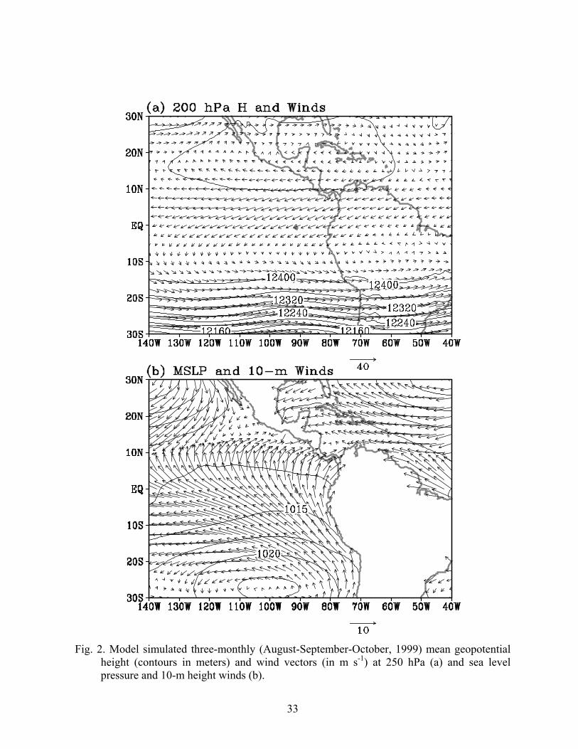
Fig. 2. Model simulated three-monthly (August-September-October, 1999) mean geopotential

height (contours in meters) and wind vectors (in m s-1) at 250 hPa (a) and sea level pressure and 10-m height winds (b).

33

Fig. 3. Three-monthly (ASO) mean daily rainfall (mm d-1) from (a) TMI observations; (b)

CMAP data; (c) model simulation (contours) with colored background showing seasonal mean SST; (d) model drizzle (mm d-1) under Sc clouds over the Southeast Pacific.

34

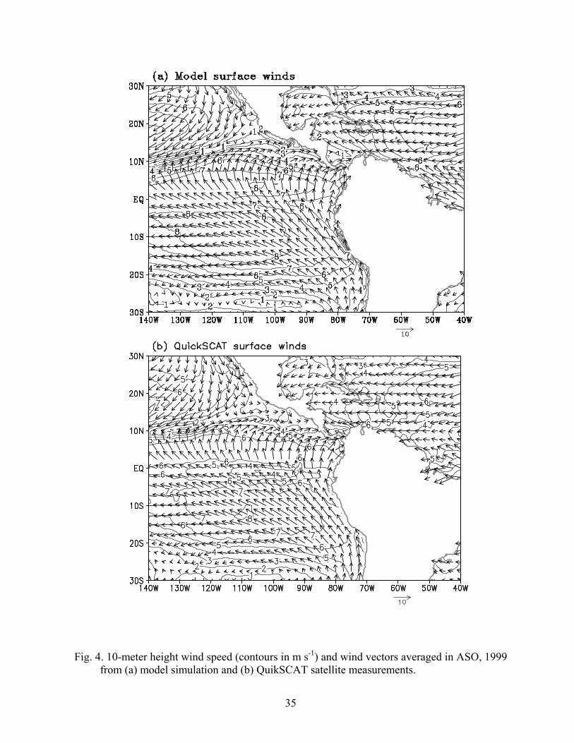
Fig. 4. 10-meter height wind speed (contours in m s-1) and wind vectors averaged in ASO, 1999

from (a) model simulation and (b) QuikSCAT satellite measurements.

35

Fig. 5. Vertically integrated cloud liquid water content (10-2 mm) averaged in ASO, 1999 from

(a) TMI observations and (b) model simulation.

36

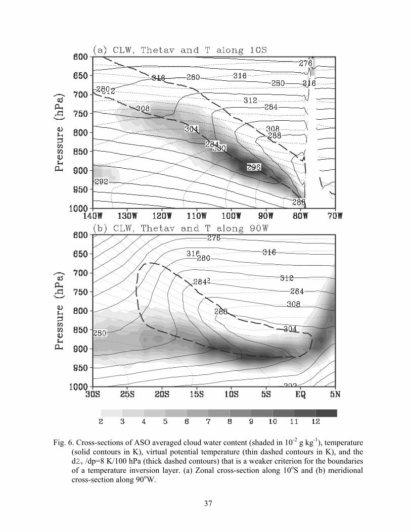
Fig. 6. Cross-sections of ASO averaged cloud water content (shaded in 10-2 g kg-1), temperature

(solid contours in K), virtual potential temperature (thin dashed contours in K), and the d2v /dp=8 K/100 hPa (thick dashed contours) that is a weaker criterion for the boundaries of a temperature inversion layer. (a) Zonal cross-section along 10oS and (b) meridional cross-section along 90oW.

37

Fig. 7. Cloud radiative forcing (CRF in W m-2) averaged in ASO. (a) Longwave CRF at the

TOA, (b) shortwave CRF at the TOA, (c) shortwave CRF at the ocean surface, (d) longwave CRF at the ocean surface. Contour intervals are 20 W m-2 in (a) and (d) and 40 W m-2 in (b) and (c).

38

Fig. 8. The net cloud radiative forcing (in W m-2) at the TOA (a) and at the ocean surface (b),

and the planetary albedo (in percentage) (c) and its component due to clouds (d) averaged in ASO. Contour intervals are 40 W m-2 in (a) and (b) and 10% in (c) and (d).

39

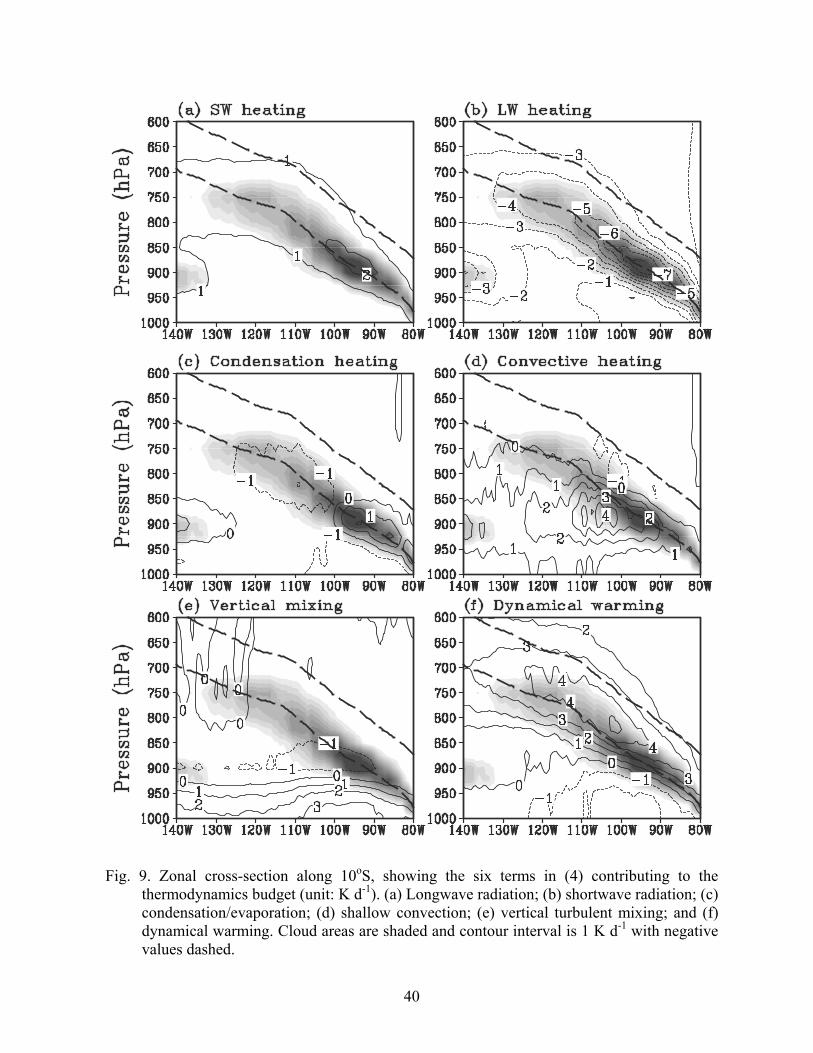
Fig. 9. Zonal cross-section along 10oS, showing the six terms in (4) contributing to the

thermodynamics budget (unit: K d-1). (a) Longwave radiation; (b) shortwave radiation; (c) condensation/evaporation; (d) shallow convection; (e) vertical turbulent mixing; and (f) dynamical warming. Cloud areas are shaded and contour interval is 1 K d-1 with negative values dashed.

40

Fig. 10. Vertical p-velocity (T in 10-2 Pa s-1) cross-sections along 10oS (a) and along 90oW (b).

Cloud areas are shaded and contour interval is 1 with negative values dashed.

41

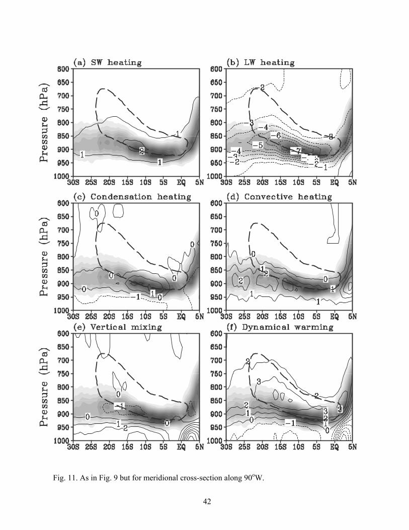
Fig. 11. As in Fig. 9 but for meridional cross-section along 90oW.

42

Fig. 12. The ASO mean boundary layer structure and the thermodynamic budget terms (K d-1)

in (4) averaged in a small box outlined by 90o-95oW and 10o-15oS. (a) Temperature (K); (b) cloud liquid water mixing ratio (10-2g kg-1); (c) Relative humidity, (d) shortwave (solid) and longwave (dashed) radiative heating rates; (e) condensational heating; (f) shallow convective heating; (g) vertical mixing; (h) dynamical warming (DW); and (i) vertical p-velocity (10-2 Pa s-1).

43

Fig. 13. Composite diurnal cycles of (a) the vertically integrated cloud water content (10-2 mm),

(b) and (c) latent and sensible heat fluxes at the sea surface (W m-2), and (d) surface wind stress (kg m-2 s-1) averaged in the same box as defined in Fig. 12.

44

12

12

12 14

Fig. 14. Vertical structure of the composite diurnal cycle, showing (a) cloud water mixing ratio (10-2g kg-1), (b) net radiative heating rate (K d-1), (c) convective heating rate (K d-1), (d) condensational/evaporative heating/cooling rate (K d-1), (e) dynamical warming (K d-1), and (f) temperature (K) averaged in the same box as defined in Fig. 12. Contour interval is 2 in all panels with negative values dashed.

45