a coupled level set–boundary integral method for …sethian/2006/papers/sethian.breaking...a...
TRANSCRIPT
Interfaces and Free Boundaries7 (2005), 1–26
A coupled level set–boundary integral method formoving boundary simulations
M. GARZON†
Department of Applied Mathematics, University of Oviedo, Oviedo, Spain
D. ADALSTEINSSON‡
Department of Mathematics, University of North Carolina, Chapel Hill, NC, USA
L. GRAY§
Computer Science and Mathematics Division, Oak Ridge National Laboratory
AND
J. A. SETHIAN¶
Department of Mathematics, University of California, Berkeley, andMathematics Department, Lawrence Berkeley National Laboratory, Berkeley, CA, USA
[Received 27 September 2004 and in revised form 12 February 2005]
A numerical method for moving boundary problems based upon level set and boundary integralformulations is presented. The interface velocity is obtained from the boundary integral solutionusing a Galerkin technique for post-processing function gradients on the interface. We introduce anew level set technique for propagating free boundary values in time, and couple this to a narrow bandlevel set method. Together, they allow us to both update the function values and the location of theinterface. The methods are discussed in the context of the well-studied two-dimensional nonlinearpotential flow model of breaking waves over a sloping beach. The numerical results show wavebreaking and rollup, and the algorithm is verified by means of convergence studies and comparisonswith previous techniques.
1. Introduction and overview
In this paper, we develop an algorithm for solving moving boundary problems. Our approachis based on a combined level set method and boundary integral method, allowing us tohandle topological changes while maintaining the highly accurate aspects of boundary integralformulations. There are many scientific and engineering areas where this capability is expectedto be important, such as free surface flows [12] and electrostatically driven flows [24, 36].
For purposes of discussion, we present the techniques in the context of wave breaking over asloping beach. This topic has been investigated extensively, both experimentally and numerically,
This work was partially supported by U.S. Department of Energy, Applied Mathematical Sciences, and the Division ofMathematical Sciences, National Science Foundation.
†E-mail:
‡E-mail:
§E-mail:
¶E-mail: [email protected]
c© European Mathematical Society 2005
2 M . GARZON ET AL.
due to the interest in surf-zone dynamics, sediment transport problems, and impact forces on off-shore and near-shore structures. The most commonly used mathematical models, based on variousassumptions, are the nonlinear shallow water equations, the nonlinear Boussinesq models and thenonlinear fully potential models (see for example [4], [15], [17], [26], [38]). More recent modelsaccount for turbulent dissipation forces generated when the wave jet overturns. These are basedon the Reynolds average Navier–Stokes equation for the mean flow and several k-ε models for theturbulent field ([19]). Slightly different approaches which also include turbulent effects can be foundin [11]. The physical validity of these various models to accurately predict wave breaking is difficultto assess, since physical experiments (Lasser doppler velocities, particle image velocity) fail to givereproducible velocity data in the roller region of the breaking wave.
Under the assumptions that water is an incompressible, inviscid fluid, the motion is irrotational,and imposing appropriate boundary conditions on the free surface, the governing equations for thewater wave motion are referred to as ‘fully nonlinear potential model’ (FNPM) and are able tomodel strongly nonlinear waves. This model has been extensively used by, for example, Grilli et al.([15], [16], [18]) to predict solitary wave shoaling and wave overturning until the jet of the waveimpinges against the flat water surface. They use a Lagrangian-Eulerian formulation of the modelequations and a high order boundary element method (BEM) to approximate the boundary integralequation for the computations of free surface velocity.
Such an approach can provide accurate solutions to wave breakage, however the numericalissues associated with regridding to maintain accuracy, topological change, complexities in threedimensions, etc., are challenging. If one considers the more general problem of two-phase flow,in which fluids (in this case, water and air) form part of the computational domain, fully Euleriantechniques for tracking the moving interface which avoid these regridding and topological issues,are available, such as level set methods, introduced by Osher and Sethian [25]. A large collection ofsimulations have been performed coupling level set methods to Chorin’s projection method ([10]) tocompute the solution of incompressible, viscous and inviscid two-phase flow, often in the presenceof interface surface tension and considerable density variation between the two fluids (see [8, 34,37, 32, 39]). In this approach, boundary conditions are required for both fluids. However, it can bedifficult to specify appropriate numerical boundary conditions for the air region in open domainsthat do not adversely affect the calculation.
2. General approach
We are interested here in problems in which a moving interface interacts with an associated partialdifferential equation describing associated physics which both transports, and is influenced by,the position of the interface. Natural candidates for this sort of motion include Hele–Shaw cells,the evolution of air bubbles in water, and electrosprays. We are interested in problems in whichtopological reconnection is possible, in which geometric terms on the interface may play importantroles, and in which issues of stability and regularization are important.
The approach taken in this paper is designed to take advantage of the well-studied robustnessand topological properties of level set methods for tracking moving interfaces, while maintainingthe accuracy, sharpness, and desirable single-fluid approach that can be obtained from a boundaryintegral formulation.
The central ideas are as follows. The interface is represented by the zero level set of an embeddedlevel set function, defined throughout a narrow band about the interface in question (see [1]).Similarly, an artificial velocity potential is defined in this region, equaling the correct velocity

MOVING BOUNDARY SIMULATIONS 3
potential along the interface. To advance the position of the interface, first a nodal representation isextracted from the level set function, as well as the velocity potential at these nodes. Then a boundaryintegral method is used to compute the velocity at each of these nodes, and this velocity is thenextended throughout the narrow band. The level set function and the velocity potential are updatedby advancing initial value Eulerian partial differential equations for both the level set function andthe velocity potential. The updating of the velocity potential is carried out using a method similar tothat in [3]. This entire process is then repeated.
The principal new features incorporated in the algorithm are (a) a fast Galerkin method forcomputing the surface gradient of the velocity potential [14]; and (b) a new level set method fortransport and diffusion of material quantities on propagating interfaces [3]. To test the algorithm, itis applied to the numerical solution of the FNPM for two-dimensional waves shoaling over flat andsloping bottoms. This approach provides a simple and direct way to solve the model equationsby reformulating the problem in a complete Eulerian framework, and straightforward upwindnumerical schemes give sufficiently accurate wave profiles while shoaling and breaking. Moreover,the algorithm is successful despite using simpler, lower order, approximations than those employedin previous work. The formulation is unchanged in three dimensions, offering the possibility ofcomputing complex breaking wave motions. We note that an early reference coupling level setmethods to boundary integral methods is [33].
Several comments are in order. To begin, although we extract the interface in order to providenodes for the boundary integral formulation, our approach should not be thought of as resting ona parametrized representation, since this discrete parametrization is used only to obtain physicalquantities which are then returned to the underlying Eulerian mesh; the discrete parametrization isthen discarded, rather than time-advanced, as is typical in Lagrangian techniques.
Second, in the example of breaking waves considered below, the formulation of the extensionpotential follows a form which we believe is a prototype for many such problems.
Third, the problem we consider in fact does not contain topological change: rather than bea limitation of the algorithm, this is a limit on the validity of the model. The model equationsfor breaking surface waves are only valid until the plunging waves impact the surface. Once thishappens, an accurate and viable model requires attention to the trapped air as well as the energydissipation that occurs due to the impact. We are currently trying to formulate a good model whichincludes these effects. We are also currently at work applying these techniques to an axisymmetricproblem in electrosprays.
3. The governing equations
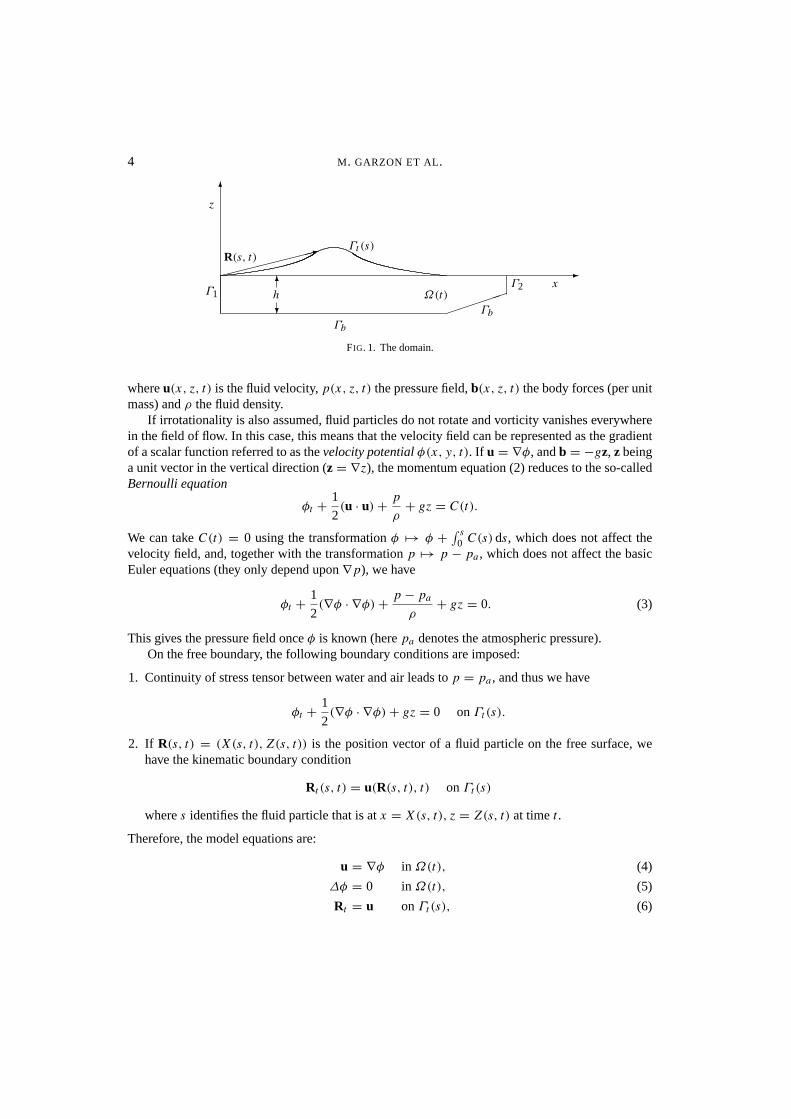
We now derive our coupled level set/extension potential equations for breaking waves. LetΩ(t) bethe 2D fluid domain in the vertical plane(x, z) at timet , with z the vertical upward direction (andz = 0 at the undisturbed free surface), andΓt (s) = (x(s, t), z(s, t)) a parametrization of the freeboundary at timet . Here,Ω(t) is the region bounded by the air/fluid interface on top, the left wall,and the sloping floor (see Figure 1).
Under the above mentioned assumptions, the mass and momentum conservation equations aregiven by
∇u = 0 inΩ(t), (1)
ut + u · ∇u =−∇p
ρ+ b in Ω(t), (2)
4 M . GARZON ET AL.
-
6
6
?hΓ1
Γb
Γb
Γ2
Γt (s)R(s, t)
Ω(t)
:
x
z
FIG. 1. The domain.
whereu(x, z, t) is the fluid velocity,p(x, z, t) the pressure field,b(x, z, t) the body forces (per unitmass) andρ the fluid density.
If irrotationality is also assumed, fluid particles do not rotate and vorticity vanishes everywherein the field of flow. In this case, this means that the velocity field can be represented as the gradientof a scalar function referred to as thevelocity potentialφ(x, y, t). If u = ∇φ, andb = −gz, z beinga unit vector in the vertical direction (z = ∇z), the momentum equation (2) reduces to the so-calledBernoulli equation
φt +1
2(u · u)+
p
ρ+ gz = C(t).
We can takeC(t) = 0 using the transformationφ 7→ φ +∫ s
0 C(s)ds, which does not affect thevelocity field, and, together with the transformationp 7→ p − pa , which does not affect the basicEuler equations (they only depend upon∇p), we have
φt +1
2(∇φ · ∇φ)+
p − pa
ρ+ gz = 0. (3)
This gives the pressure field onceφ is known (herepa denotes the atmospheric pressure).On the free boundary, the following boundary conditions are imposed:
1. Continuity of stress tensor between water and air leads top = pa , and thus we have
φt +1
2(∇φ · ∇φ)+ gz = 0 onΓt (s).
2. If R(s, t) = (X(s, t), Z(s, t)) is the position vector of a fluid particle on the free surface, wehave the kinematic boundary condition
Rt (s, t) = u(R(s, t), t) onΓt (s)
wheres identifies the fluid particle that is atx = X(s, t), z = Z(s, t) at timet .
Therefore, the model equations are:
u = ∇φ in Ω(t), (4)
∆φ = 0 inΩ(t), (5)
Rt = u onΓt (s), (6)
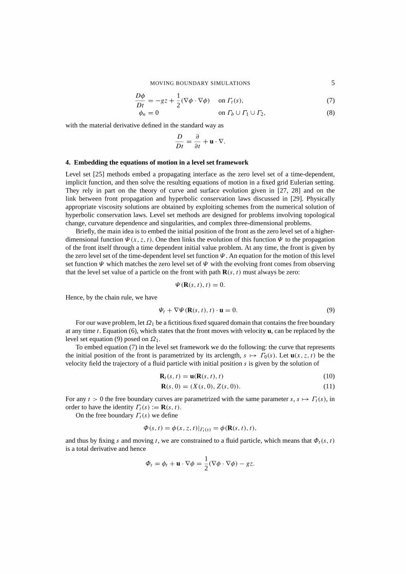
MOVING BOUNDARY SIMULATIONS 5
Dφ
Dt= −gz+
1
2(∇φ · ∇φ) onΓt (s), (7)
φn = 0 onΓb ∪ Γ1 ∪ Γ2, (8)
with the material derivative defined in the standard way as
D
Dt=∂
∂t+ u · ∇.
4. Embedding the equations of motion in a level set framework
Level set [25] methods embed a propagating interface as the zero level set of a time-dependent,implicit function, and then solve the resulting equations of motion in a fixed grid Eulerian setting.They rely in part on the theory of curve and surface evolution given in [27, 28] and on thelink between front propagation and hyperbolic conservation laws discussed in [29]. Physicallyappropriate viscosity solutions are obtained by exploiting schemes from the numerical solution ofhyperbolic conservation laws. Level set methods are designed for problems involving topologicalchange, curvature dependence and singularities, and complex three-dimensional problems.
Briefly, the main idea is to embed the initial position of the front as the zero level set of a higher-dimensional functionΨ (x, z, t). One then links the evolution of this functionΨ to the propagationof the front itself through a time dependent initial value problem. At any time, the front is given bythe zero level set of the time-dependent level set functionΨ . An equation for the motion of this levelset functionΨ which matches the zero level set ofΨ with the evolving front comes from observingthat the level set value of a particle on the front with pathR(s, t) must always be zero:
Ψ (R(s, t), t) = 0.
Hence, by the chain rule, we have
Ψt + ∇Ψ (R(s, t), t) · u = 0. (9)
For our wave problem, letΩ1 be a fictitious fixed squared domain that contains the free boundaryat any timet . Equation (6), which states that the front moves with velocityu, can be replaced by thelevel set equation (9) posed onΩ1.
To embed equation (7) in the level set framework we do the following: the curve that representsthe initial position of the front is parametrized by its arclength,s 7→ Γ0(s). Let u(x, z, t) be thevelocity field the trajectory of a fluid particle with initial positions is given by the solution of
Rt (s, t) = u(R(s, t), t) (10)
R(s,0) = (X(s,0), Z(s,0)). (11)
For anyt > 0 the free boundary curves are parametrized with the same parameters, s 7→ Γt (s), inorder to have the identityΓt (s) := R(s, t).
On the free boundaryΓt (s) we define
Φ(s, t) = φ(x, z, t)|Γt (s) = φ(R(s, t), t),
and thus by fixings and movingt , we are constrained to a fluid particle, which means thatΦt (s, t)
is a total derivative and hence
Φt = φt + u · ∇φ =1
2(∇φ · ∇φ)− gz.
6 M . GARZON ET AL.
Next, letG(x, z, t) be a function defined onΩ1 with the following property:
G(X(s, t), Z(s, t), t) = Φ(s, t) onΓt (s). (12)
It is important to remark here thatG(x, z, t) is an auxiliary function which can be chosen arbitrarily,with the only restriction to be equal toφ(x, z, t) on Γt (s). Applying the chain rule in the identity(12) we obtain
Gt + u · ∇G =1
2(∇φ · ∇φ)− gz, (13)
which holds onΓt (s). Note thatu and the right hand side of (13) are only defined onΓt (s). In orderto be able to solve (13) over the whole domainΩ1, we need to extend these variables off the front;this strategy is discussed below.
The model equations, written in a complete Eulerian framework, are
u = ∇φ in Ω(t), (14)
∆φ = 0 inΩ(t), (15)
Ψt + uext · ∇Ψ = 0 inΩ1, (16)
Gt + uext · ∇G = fext in Ω1, (17)
φn = 0 onΓb ∪ Γ1 ∪ Γ2, (18)
wheref =12(∇φ · ∇φ)− gz andfext anduext are the extensions off andu ontoΩ1.
5. Numerical approximations and algorithms
In this section, we provide overviews of the various components. More detailed discussions of levelset methods, boundary element methods, fast extension velocities, potential initializations, may befound in the cited references.
5.1 Initialization
The initial front positionΓ0(s) = (x(s,0), z(s,0)) and initial velocity potentialφ(x, z,0)|Γ0(s)
are needed to solve equations (16) and (17) respectively. Given an initial solitary wave amplitude(H0) and the physical length of the domain (L), Tanaka’s method gives a way of calculating thesequantities (for this aim we have used the Fortran code kindly provided by S. T. Grilli). Here, webriefly discuss the theoretical basis of this method.
Assuming constant depth, the flow field can be reduced to steady state by using a coordinatesystem that moves horizontally with speed equal to the wave celerityc. The stream functionψ(x, z)is also harmonic and takes constant values at the bottom and at the free surface of the domain. Fromthe definition of stream function and velocity potential we have
φx = ψy, φy = −ψx .
Under sensible assumptions about the smoothness ofφ andψ , these are just the Cauchy–Riemannequations which are satisfied by the real and imaginary parts of the functionW = φ+ iψ , called thecomplex potential, which is an analytic function of the complex variableZ = x + iz in the domain
MOVING BOUNDARY SIMULATIONS 7
occupied by the fluid. By interchanging the roles of the variablesZ andW , we can takeφ andψas independent variables, sinceW = φ + iψ provides a one-to-one correspondence between thephysical and complex potential planes. With this transformation, the fluid region is mapped into thestrip 0< ψ < 1, −∞ < φ < ∞ in theW plane withψ = 1 on the free surface,ψ = 0 on thebottom andφ = 0 at the wave crest. Denote byu, v the horizontal and vertical components of thevelocity u, q = |u| andθ the angle between the velocity and thex-axis. The complex velocity isdefined by
dW
dZ= φx + iφy = u− iv = qeiθ
and it is also analytic in the flow domain. Therefore, the quantity
ω = ln
(dW
dZ
)= ln q − iθ
is an analytic function ofW , soτ = ln q must be harmonic in the strip 0< ψ < 1, −∞ < φ < ∞.The Bernoulli condition at the free surface and the bottom condition can be expressed in terms ofq
andθ as
dq3
dφ= −
3
F 2sinθ onψ = 1, (19)
θ = 0 onψ = 0, (20)
whereF is the Froude number defined byF = c/√gh.
The problem of finding a solitary wave solution can thus be transformed into the problem offinding a complex functionω that is analytic with respect toW within the unit strip 0< ψ < 1,decays at infinity, and satisfies the boundary conditions (19) and (20). Tanaka’s method providesa way to solve the previously outlined equations in terms of the new variablesτ , θ , and a fulldescription of the algorithm can be found in [35].
5.2 Level set methods
We use the standard narrow band level method, introduced by Adalsteinsson and Sethian [2], whichlimits computation to a thin band around the front of interest. Following the algorithm discussedin [25], we use second order in space upwind differences to approximate the gradient in the levelset equation, and a first order in time scheme to update the solution. For boundary conditions,homogeneous flux boundary conditions are usually chosen, which are implemented by creatingan extra layer of ghost cells around the domain whose values are simply direct copies of theΨ
values along the actual boundary. The level set function is built from the initial position of the frontby computing the signed distance function. This is done by using the fast marching method [30],which is a Dijkstra-like finite difference method for computing the solution to the eikonal equationin O(N logN), whereN is the total number of points in the computational domain.
The velocity and the velocity potential are both initially defined only on the interface. In orderto create values throughout the narrow band, which are required to update the fixed grid Eulerianpartial differential equations, we use the extension methodology developed by Adalsteinsson andSethian in [2] to construct appropriate extensions. The idea of building extension velocities was firstintroduced in [20]; in that approach, the extension velocity at any grid point in the domain was taken

8 M . GARZON ET AL.
as equal to the velocity at the closest point on the front itself. As shown in [7], this is equivalent tosolving the equation∇Vi · ∇Ψ = 0 (i = 1,2) for the velocity components, and in that paper, theequation was solved using a finite difference iteration. In [2], Adalsteinsson and Sethian present atechnique for computing this extension velocity using the very efficient fast marching methodology.Finally, in [3], this approach was developed to build extension values for arbitrary material quantitieswhose evolution affects the underlying interface dynamics.
5.3 The boundary integral equation and the BEM approximation
A first order boundary element method is used to approximate equation (15). Boundary integralequations are well suited to moving boundary problems for two principal reasons. First, determiningthe surface velocity generally requires computing function derivatives on this boundary, which areaccurately evaluated within this formulation. Second, remeshing the moving boundary is clearlysimpler than remeshing the entire domain.
The Laplace equation for the velocity potential (15) is solved by approximating thecorresponding boundary integral equation. Boundary conditions are given by (18) and, on the freeboundary, at each time step, by the updated potential velocity given by equation (17). Again, on thefree surface,φ is known (or more accurately, is computed by the level set method), and the boundaryelement method is used to compute∂φ/∂n. However, we do not need the potential on the side wallsin order to advance the wave, and thus this part of the solution is ignored. The approximation of theintegral equation is done by the BEM, which calculates the potential and the potential gradient onthe free surface, that is, its velocityu.
The boundary integral equation for the potentialφ(P ), in a domainΩ(t) having boundaryΣ =
∂Ω(t), can be written as
P(P ) = φ(P )+ limPI→P
∫Σ
[φ(Q)
∂G∂n(PI ,Q)− G(PI ,Q)
∂φ
∂n(Q)
]dQ = 0, (21)
wheren = n(Q) denotes the unit outward normal on the boundary surface andPI are interiorpoints converging to the boundary pointP . The Green’s function or fundamental solution (in twodimensions) is
G(P,Q) = −1
4πlog(r). (22)
The integral equation is usually written with the∂G/∂n singular integral evaluated as a Cauchyprincipal value (CPV), resulting in an ‘interior angle’ coefficientc(P )multiplying the leadingφ(P )term [5, 6]. The reason for employing the seemingly more complicated limit process will becomeclear in the discussion of gradient evaluation. The exterior limit equation
limPE→P
∫Σ
[φ(Q)
∂G∂n(PE,Q)− G(PE,Q)
∂φ
∂n(Q)
]dQ = 0 (23)
yields precisely the same equation: the jump in the CPV integral as one crosses the boundaryaccounts for the ‘free term’ difference.
In this work, a Galerkin (weak form) approximation of (21) has been employed, and theboundary and boundary functions are interpolated using the simplest approximation, linear shapefunctions. Thus, the equations that are solved are of the form∫
Σ
ψk(P )P(P )dP = 0, (24)
MOVING BOUNDARY SIMULATIONS 9
where the weight functionsψk(P ) are comprised of all shape functions which are nonzero at aparticular nodePk (cf. [5]). The calculations reported herein employed the simplest approximation,linear shape functions. These approximations reduce the integral equation to a finite system oflinear equations, and invoking the boundary conditions allows the solution of the unknown values ofpotential and flux on the boundary. Details concerning the limit evaluation of the singular integralscan be found in [13].
As noted above, for the wave problem, and moving boundary problems in general, knowledgeof the normal flux is not sufficient: we may need both velocity components with respect to theCartesian coordinates. Note that in (16) the separate Cartesian components of the velocity are whatappears, not the flux. What we are required to do is to compute a post-boundary-element solve inorder to find these individual components.
The remainder of this section will present the algorithm for computing this gradient.From (21) a gradient component can be expressed as
∂φ(P )
∂Ek= limPI→P
∫Σ
[∂G∂Ek
(PI ,Q)∂φ
∂n(Q)− φ(Q)
∂2G∂Ek∂n
(PI ,Q)
]dQ. (25)
Once the boundary value problem has been solved, all quantities on the right hand side are known: adirect evaluation of nodal derivatives would therefore be easy were it not for well known difficultieswith the hypersingular (two derivatives of the Green’s function) integral [22, 23, 21]. As describedin [14], a Galerkin approximation of this equation,∫
Σ
ψk(P )∂φ(P )
∂EkdP
= limPI→P
∫Σ
ψk(P )
∫Σ
[∂G∂Ek
(PI ,Q)∂φ
∂n(Q)− φ(Q)
∂2G∂Ek∂n
(PI ,Q)
]dQdP, (26)
allows a treatment of the hypersingular integral using standard continuous elements.Interpolating∂φ(P )/∂Ek as a linear combination of the shape functions results in a simple
system of linear equations for nodal values of the derivative everywhere onΣ ; the coefficient matrixis obtained by simply integrating products of two shape functions. However, the complete boundaryintegrations required to compute the right hand side are quite expensive.
The computational cost of this procedure can be significantly reduced by exploiting the exteriorlimit equation, (23). It appears to be useless for computing tangential derivatives for, lacking thefree term, the corresponding derivative equation takes the form
0 = limPE→P
∫Σ
[∂G∂Ek
(PE,Q)∂φ
∂n(Q)− φ(Q)
∂2G∂Ek∂n
(PE,Q)
]dQ, (27)
and the derivatives obviously do not appear. However, subtracting this equation from (25) yields(with shorthand notation)
∂φ(P )
∂Ek= lim
PI→P− limPE→P
∫Σ
[∂G∂Ek
∂φ
∂n(Q)− φ(Q)
∂2G∂Ek∂n
]dQ. (28)
The advantage of this formulation is that nowonly the terms that are discontinuous crossingboundarycontribute to the integral. In particular, all nonsingular integrations, by far the most time
10 M . GARZON ET AL.
consuming, drop out. The calculation of the right hand side in (28) reduces to a few ‘local’ singularintegrations, and as these integrations are carried out partially analytically, this produces an accuratealgorithm. Further details about the evaluation of (28) can be found in [14].
5.4 The velocity potential updating
The potential equation (17) is a convection equation with a strong nonlinear source term, andhomogeneous Neumann boundary conditions are imposed on the boundary ofΩ1. To update intime this equation, note that it is similar to (16) except that it has a nonlinear source term, andtherefore we use similar schemes. For example a straightforward first order scheme is
Gn+1i,j = Gni,j −∆t(max(uni,j ,0)D
−xi,j + min(uni,j ,0)D
+xi,j
+ max(vni,j ,0)D−zi,j + min(vni,j ,0)D
+zi,j )+∆tf ni,j
where
D−xi,j = D−x
i,j Gni,j =
Gni,j −Gni−1,j
∆x, D+x
i,j = D+xi,j G
ni,j =
Gni+1,j −Gni,j
∆x
are the backward and forward finite approximations for the derivative in thex direction (we havethe same expressions forD−z
i,j andD+zi,j ). Note that for simplicity we have writtenu, v, f instead
of uext, vext, fext, and we describe a first order explicit scheme with a centered source term. Initialvalues ofG0
i,j are obtained by extendingφ(x, z,0)|Γ0(s) as previously discussed. However, at anytime stepn it is always possible to perform a new extension ofΦn(s, n∆t) to obtain a better valueof Gni,j .
A key issue is how one obtainsfext at the grid points ofΩ1. There are several ways of doing so.Here we calculatef =
12(∇φ ·∇φ)−gz on free surface nodes, and use these values together with the
condition∇f · ∇Ψ = 0 to obtainfext. This algorithm for extending off the front quantities definedon the front works very well for the velocity field in the case of equation (16), as it maintains thesigned distance function for the level sets ofΨ . However, regarding equation (17) for this particularwave problem, the previous method creates strongG andf gradients inΩ1. This is due to the highvariations off along the front together with its topological structure when overturning. This factlimits the grid spacing inΩ1 and the time step needed to maintain accuracy (see the section onnumerical experiments).
5.5 Regridding of the free surface
In a level set formulation the position of the front is only known implicitly through the node values ofthe level set functionΨ . In order to extract the front, it is possible to construct first order and secondorder approximations of the interface using local data ofΨ on the mesh (see [9] for example). Herewe use a first order linear approximation of the free surface, which yields a polygonal interfaceformed by unevenly distributed nodes, which we call LS nodes. As a result of this extractiontechnique, we can sometimes get front nodes which are very close together, and this can causedifficulties and instabilities for boundary element calculations. To overcome this problem, and alsoto achieve more front resolution when needed, we employed a front node regridding technique. Aninitialization point on the front is selected according to a particular criterion, such as maximumvalue of height, velocity modulus, or front curvature. This point divides the front into two halves
MOVING BOUNDARY SIMULATIONS 11
and new nodes are chosen so that, lying in the same polygon, they are redistributed by arclengthaccording to the formula
si+1 − si = d0(1 + si(f0 − 1))
wheresi denotes the arclength distance from nodei to the initialization point (i = 0), andd0, f0 areuser selected parameters. These regridded nodes on the front are used to create the input file for theBEM calculations and are denoted by BEM nodes.
5.6 The algorithm
To initialize the position of the front and the velocity potential on the front, we use Tanaka’s methodfor computing numerical exact solitary waves.
The basic algorithm can be summarized as follows:
1. Compute the initial front position and velocity potentialΦ(s,0) onΓ0(s).
2. ExtendΦ(s,0) onto the grid points ofΩ1 to initializeG.3. GenerateΩ(t) and solve (15), using the boundary element method. This yields the velocityu
and source termf at the front nodes.4. Extendu andf off the front ontoΩ1.5. UpdateG using (17) inΩ1.6. Move the front with velocityu using (16) inΩ1.7. Interpolate (bicubic interpolation)G from grid points ofΩ1 to the front nodes to obtain new
boundary conditions for(15). Go back to step 3 and repeat forward in time.
A more detailed algorithm including regridding is:
Initialization: GivenΓ 0= Γ0(s),Φ
0= Φ(s,0)
1. CalculateΨ 0 and LS nodes.2. ExtendΦ0 to obtainG0.3. Redistribute LS nodes to obtain BEM nodes.4. Calculateu0 at BEM nodes.5. Findu0 andf 0 at LS nodes and extend ontoΩ1.
Steps: GivenΨ n, Φn,un
1. CalculateΨ n+1 and LS nodes.2. CalculateGn+1 atΩ1 grid points.3. Redistribute LS nodes to obtain BEM nodes.4. InterpolateG on BEM nodes to findΦn+1.5. Calculateun+1 at BEM nodes.6. Findun+1 andf n+1 at LS nodes and extend ontoΩ1. Go to step 1 and repeat.7. If reinitialization
(a) Take LS nodes and reinitializeΨ n+1.(b) Take BEM nodes and extendΦn+1.
5.7 Numerical accuracy
The model equations imply that the wave mass and its total energy should be conserved as the waveevolves in time. One way to check the numerical accuracy of the discretized equations is to compute
12 M . GARZON ET AL.
these quantities at each time step (here, we are checking the conservation of energy to see how itdepends on grid resolution). The wave mass abovez = 0 is given by
m(t) =
∫Ω(t)
dΩ =
∫∂Ω(t)
znz ds =
∫Γt (s)
znz ds
and the total energy isE(t) = Ep(t) + Ek(t), whereEp(t), Ek(t) denote the potential and kineticwave energy respectively. They can be calculated using the expressions
Ep(t) =1
2ρg
∫Ω(t)
z dΩ =1
2ρg
∫Γt (s)
z2nz ds,
which is the potential energy with respect toz = 0, and
Ek(t) =1
2ρ
∫Ω(t)
∇φ · ∇φ dΩ =1
2ρ
∫∂Ω(t)
φ∂φ
∂nds =
1
2ρ
∫Γt (s)
φ∂φ
∂nds,
where the divergence theorem has been applied to the three formulas and we have used the factthat∂φ/∂n = 0 onΓb, Γ1, Γ2 for the kinetic energy formula. These integrals are approximated bya composite trapezoidal rule, using the values of the quantities at the free boundary BEM nodes.Note that LS nodes could have been used form(t) andEp(t) approximations but we also used BEMnodes for simplicity. The components of the normal vector to the free surface are computed usingthe level set embedding function to obtain surface geometrical variables.
A common procedure to study the accuracy and convergence properties of the discretizedequations with respect to the mesh sizes and the time step is by means of an analytical solution.A solitary wave propagating over a constant depth is a traveling wave that moves in thex directionwith speed equal to the celerity of the wave (c). The velocity potential and the velocity on the frontas functions ofx are also translated with the same speedc. Therefore, in this case, by calculatinginitial wave data with Tanaka’s method and translating it, we are able to compute theL2 norms of theerrors for the various magnitudes. For the case of a solitary wave shoaling over a sloping bottom, theaccuracy can only be checked looking at the mass and energy conservation properties and comparingbreaking wave characteristics obtained here with those reported elsewhere, for example in [16].
6. Numerical results
The system of equations to be discretized is a nonlinear system of strongly coupled partialdifferential equations. First order in time and second order in space schemes are used for equation(16); first order in time and in space schemes are used for equation (17); and a first order BEMsolver is used for the velocity updating.
To study the convergence properties of this method and its capability to predict wave breakingcharacteristics, the numerical results corresponding to the following physical settings are presented:A solitary wave propagating over a constant depth and the shoaling and breaking of a solitary wavepropagating over various sloping bottoms.
6.1 Constant depth test
In order to tune the discretization parameters and see how they affect numerical accuracy weperformed a series of numerical tests with a solitary wave ofH0 = 0.5 m (wave height at the
MOVING BOUNDARY SIMULATIONS 13
crest) propagating over a constant depth of 1 m. The wave crest is initially located atx = 6.5 m andthe domain hasL = 15 m of length. In what follows, the units are taken as meters and seconds forlength and time, respectively.
Let Ω1 = [0,15] × [−0.3,1] be the fictitious domain that contains the free boundary for allt ∈ [0,0.5],∆x = ∆z the grid size and∆t the time step. To discretize∂Ω(t), in order to generatethe input BEM file, a variable mesh size is used:∆l = 0.1 for Γ1 andΓ2,∆l = 0.2 for Γb, and theregridding parameters forΓs(t) are chosen to bed0 = 0.005,f0 = 10. This gives 193 BEM nodeson the moving front and 98 nodes on the fixed boundaries.
The mesh size∆x = ∆z for Ω1 should be chosen in order to achieve accurate interpolatedvalues of front position and potential on the front. For the time step selection, a first limitation is theCFL condition. While this condition is enough for the stability of the numerical approximation ofequations (16) and (17), the accuracy in the numerical solution of equation (17) requires a smallertime step. This is due to the fact thatG and the source termf , for this particular wave problem,develop high gradients inΩ1. Therefore we present the results for the following test cases:
(a) ∆x = 0.1,∆t = 0.01.(b) ∆x = 0.1,∆t = 0.001.(c) ∆x = 0.01,∆t = 0.001.(d) ∆x = 0.01,∆t = 0.0001.
For given solitary wave parameters (H0 and lengthL in thex direction) Tanaka’s method givesus the initial wave magnitudes, front location, velocity potential, velocity components at front pointsand wave celerityc. At any time t , let (xex, zex), φex , uex , vex be the values of these variablesobtained by translating initial values a distancect along thex direction and spline interpolatingat LS nodes. Denote by(xc, zc), φc, uc, vc the computed values at LS nodes, and byL2(z)
= ‖zc − zex‖L2(Γs (t)), L2(φ) = ‖φc − φex‖L2(Γs (t)), L2(u) = ‖uc − uex‖L2(Γs (t)) andL2(v) =
‖vc − vex‖L2(Γs (t)) theL2 norms of the errors. Table 1 shows these errors at the final timet = 0.5for the various test cases.
TABLE 1Values of theL2 error norms att = 0.5
Test L2(z) L2(φ) L2(u) L2(v)
(a) 0.007239 0.095254 0.025147 0.025856(b) 0.009762 0.021451 0.039635 0.035685(c) 0.001476 0.011363 0.0099744 0.009356(d) 0.001699 0.00424601 0.0106674 0.010188
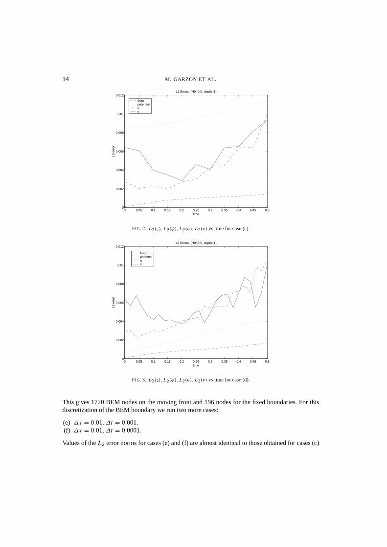
Figures 2 and 3 showL2(z), L2(φ), L2(u), L2(v) versus time for cases (c) and (d) respectively.As observed from these results, theL2 error norm in front location and velocity componentsdecreases with mesh size (∆x) but not with the time step. Only the velocity potential gains accuracywhen∆t is reduced according to the above mentioned facts.
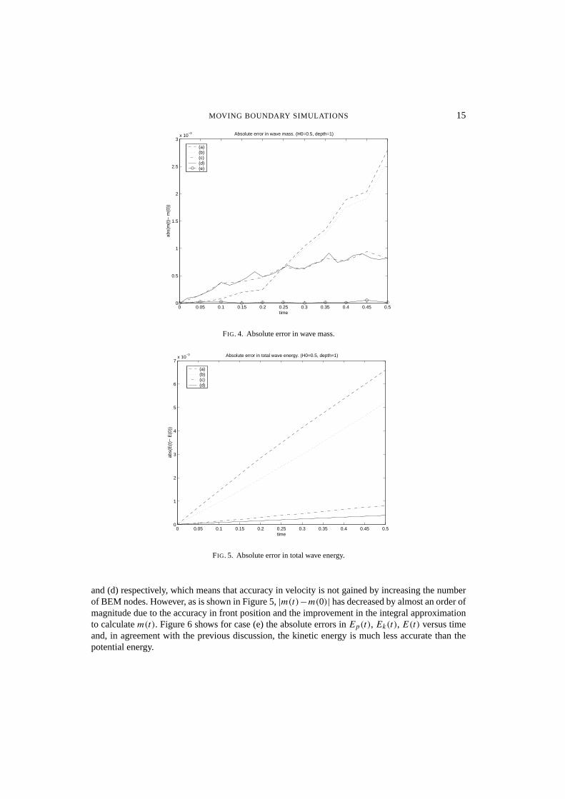
Regarding wave mass and energy conservation, at each time step we calculatem(t) andE(t) asexplained in 4.7. Figures 4 and 5 show the values of|m(t) − m(0)| and|E(t) − E(0)| versus timeand the same behavior of these quantities with respect discretization parameters is observed.
Next, to see if we gain accuracy in the velocity calculations by increasing the number of BEMnodes, we take∆l = 0.05 onΓ1 andΓ2, ∆l = 0.1 onΓb, andd0 = 0.001,f0 = 5 onΓs(t).
14 M . GARZON ET AL.
0 0.05 0.1 0.15 0.2 0.25 0.3 0.35 0.4 0.45 0.50
0.002
0.004
0.006
0.008
0.01
0.012L2 Errors. (H0=0.5, depth=1)
time
L2 e
rror
frontpotentialuv
FIG. 2. L2(z), L2(φ), L2(u), L2(v) vs time for case (c).
0 0.05 0.1 0.15 0.2 0.25 0.3 0.35 0.4 0.45 0.50
0.002
0.004
0.006
0.008
0.01
0.012L2 Errors. (H0=0.5, depth=1)
time
L2 e
rror
frontpotentialuv
FIG. 3. L2(z), L2(φ), L2(u), L2(v) vs time for case (d).
This gives 1720 BEM nodes on the moving front and 196 nodes for the fixed boundaries. For thisdiscretization of the BEM boundary we run two more cases:
(e) ∆x = 0.01,∆t = 0.001.(f) ∆x = 0.01,∆t = 0.0001.
Values of theL2 error norms for cases (e) and (f) are almost identical to those obtained for cases (c)
MOVING BOUNDARY SIMULATIONS 15
0 0.05 0.1 0.15 0.2 0.25 0.3 0.35 0.4 0.45 0.50
0.5
1
1.5
2
2.5
3x 10
−3 Absolute error in wave mass. (H0=0.5, depth=1)
time
abs(
m(t
)− m
(0))
(a)(b)(c)(d)(e)
FIG. 4. Absolute error in wave mass.
0 0.05 0.1 0.15 0.2 0.25 0.3 0.35 0.4 0.45 0.50
1
2
3
4
5
6
7x 10
−3 Absolute error in total wave energy. (H0=0.5, depth=1)
time
abs(
E(t
)− E
(0))
(a)(b)(c)(d)
FIG. 5. Absolute error in total wave energy.
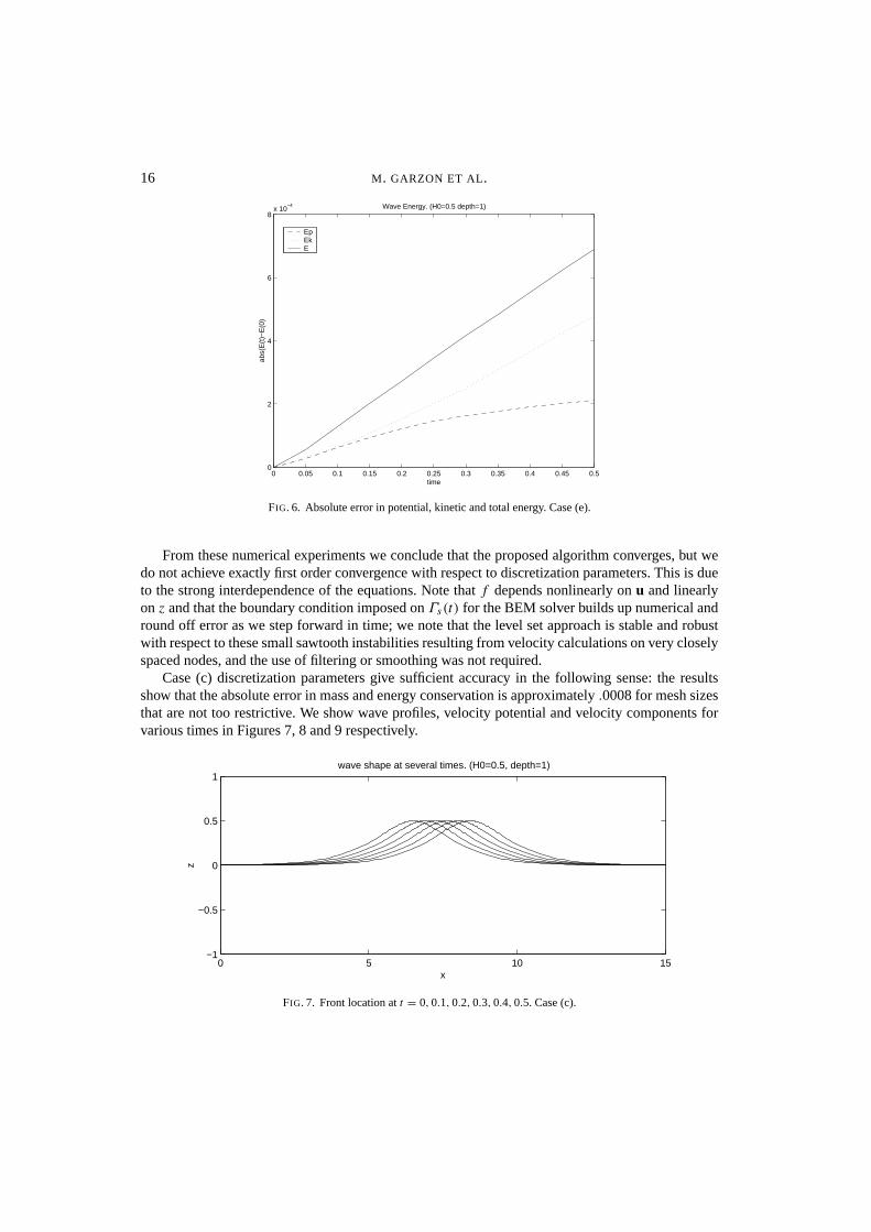
and (d) respectively, which means that accuracy in velocity is not gained by increasing the numberof BEM nodes. However, as is shown in Figure 5,|m(t)−m(0)| has decreased by almost an order ofmagnitude due to the accuracy in front position and the improvement in the integral approximationto calculatem(t). Figure 6 shows for case (e) the absolute errors inEp(t), Ek(t), E(t) versus timeand, in agreement with the previous discussion, the kinetic energy is much less accurate than thepotential energy.
16 M . GARZON ET AL.
0 0.05 0.1 0.15 0.2 0.25 0.3 0.35 0.4 0.45 0.50
2
4
6
8x 10
−4 Wave Energy. (H0=0.5 depth=1)
time
abs(
E(t
)−E
(0)
EpEkE
FIG. 6. Absolute error in potential, kinetic and total energy. Case (e).
From these numerical experiments we conclude that the proposed algorithm converges, but wedo not achieve exactly first order convergence with respect to discretization parameters. This is dueto the strong interdependence of the equations. Note thatf depends nonlinearly onu and linearlyonz and that the boundary condition imposed onΓs(t) for the BEM solver builds up numerical andround off error as we step forward in time; we note that the level set approach is stable and robustwith respect to these small sawtooth instabilities resulting from velocity calculations on very closelyspaced nodes, and the use of filtering or smoothing was not required.
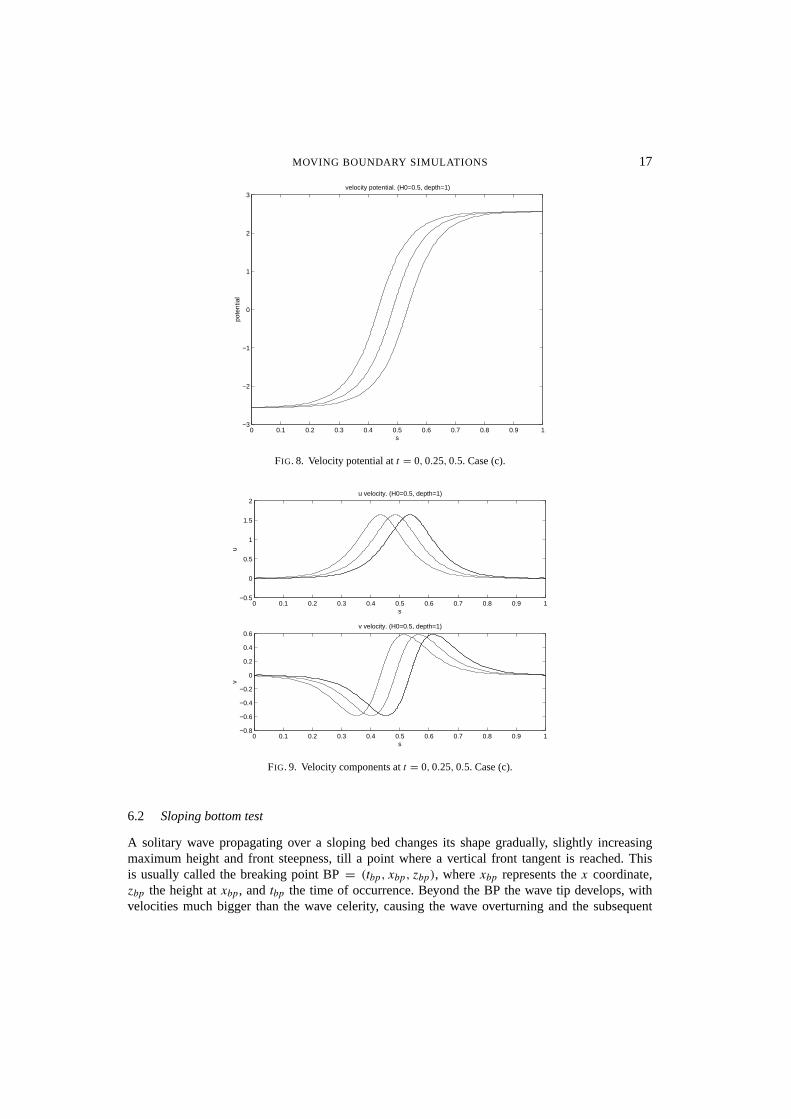
Case (c) discretization parameters give sufficient accuracy in the following sense: the resultsshow that the absolute error in mass and energy conservation is approximately.0008 for mesh sizesthat are not too restrictive. We show wave profiles, velocity potential and velocity components forvarious times in Figures 7, 8 and 9 respectively.
0 5 10 15−1
−0.5
0
0.5
1wave shape at several times. (H0=0.5, depth=1)
x
z
FIG. 7. Front location att = 0,0.1,0.2,0.3,0.4,0.5. Case (c).
MOVING BOUNDARY SIMULATIONS 17
0 0.1 0.2 0.3 0.4 0.5 0.6 0.7 0.8 0.9 1−3
−2
−1
0
1
2
3velocity potential. (H0=0.5, depth=1)
s
pote
ntia
l
FIG. 8. Velocity potential att = 0,0.25,0.5. Case (c).
0 0.1 0.2 0.3 0.4 0.5 0.6 0.7 0.8 0.9 1−0.5
0
0.5
1
1.5
2u velocity. (H0=0.5, depth=1)
s
u
0 0.1 0.2 0.3 0.4 0.5 0.6 0.7 0.8 0.9 1−0.8
−0.6
−0.4
−0.2
0
0.2
0.4
0.6v velocity. (H0=0.5, depth=1)
s
v
FIG. 9. Velocity components att = 0,0.25,0.5. Case (c).
6.2 Sloping bottom test
A solitary wave propagating over a sloping bed changes its shape gradually, slightly increasingmaximum height and front steepness, till a point where a vertical front tangent is reached. Thisis usually called the breaking point BP= (tbp, xbp, zbp), wherexbp represents thex coordinate,zbp the height atxbp, andtbp the time of occurrence. Beyond the BP the wave tip develops, withvelocities much bigger than the wave celerity, causing the wave overturning and the subsequent
18 M . GARZON ET AL.
TABLE 2Breaking characteristics
Test tbp xbp zbp tep xep
(a) 2.76 17.39 0.674 3.36 20.2(b) 2.34 15.20 0.662 2.90 17.8
falling of the jet toward the flat water surface. Denote this endpoint as EP= (tep, xep, zep). Totalwave mass and total energy should be theoretically conserved until EP. However beyond the BP, aloss in potential energy and the corresponding gain in kinetic energy is expected, due to the largevelocities on the wave jet.
Wave breaking characteristics change, mainly according to initial wave amplitude(H0) andbottom topography. To study how our numerical method predicts wave breaking we run thefollowing test cases:
(a) H0 = 0.6,L = 25, slope= 1 : 22,xc = 6.05,xs = 6,(b) H0 = 0.6,L = 18, slope= 1 : 15,xc = 5.55,xs = 5.4,
and compare the results obtained here for case (b) with those reported in [15]. Herexc denotes thex coordinate at the crest for the initial wave, andxs thex coordinate where the bottom slope starts.
A series of numerical experiments have been made, and optimal discretization parameters foundare:∆x = 0.01,∆t = 0.0001 andd0 = 0.005,f0 = 10 (approximately 193 BEM nodes) for allcases. Front regridding has been made according to maximum height before the BP and accordingto maximum velocity modulus beyond BP. Beyond the BP, and due to the complex topography ofthe wave front, reinitialization ofΨ and newΦ(s, t) extension has been performed every 1000 timesteps.
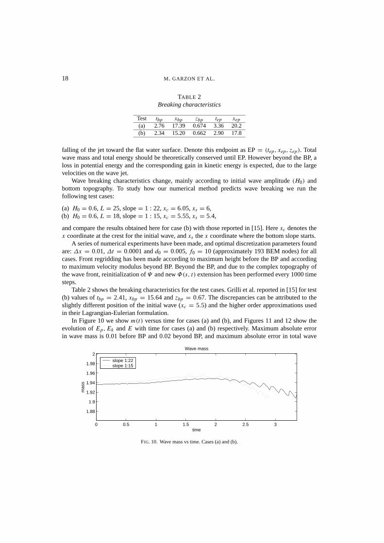
Table 2 shows the breaking characteristics for the test cases. Grilli et al. reported in [15] for test(b) values oftbp = 2.41, xbp = 15.64 andzbp = 0.67. The discrepancies can be attributed to theslightly different position of the initial wave (xc = 5.5) and the higher order approximations usedin their Lagrangian-Eulerian formulation.
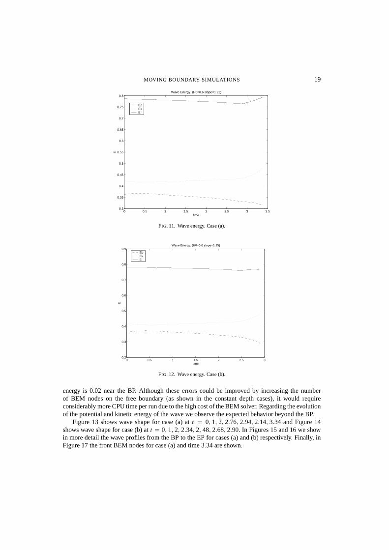
In Figure 10 we showm(t) versus time for cases (a) and (b), and Figures 11 and 12 show theevolution ofEp, Ek andE with time for cases (a) and (b) respectively. Maximum absolute errorin wave mass is 0.01 before BP and 0.02 beyond BP, and maximum absolute error in total wave
0 0.5 1 1.5 2 2.5 3
1.88
1.9
1.92
1.94
1.96
1.98
2Wave mass
time
mas
s
slope 1:22slope 1:15
FIG. 10. Wave mass vs time. Cases (a) and (b).
MOVING BOUNDARY SIMULATIONS 19
0 0.5 1 1.5 2 2.5 3 3.50.3
0.35
0.4
0.45
0.5
0.55
0.6
0.65
0.7
0.75
0.8Wave Energy. (H0=0.6 slope=1:22)
time
E
EpEkE
FIG. 11. Wave energy. Case (a).
0 0.5 1 1.5 2 2.5 30.2
0.3
0.4
0.5
0.6
0.7
0.8
0.9Wave Energy. (H0=0.6 slope=1:15)
time
E
EpEkE
FIG. 12. Wave energy. Case (b).
energy is 0.02 near the BP. Although these errors could be improved by increasing the numberof BEM nodes on the free boundary (as shown in the constant depth cases), it would requireconsiderably more CPU time per run due to the high cost of the BEM solver. Regarding the evolutionof the potential and kinetic energy of the wave we observe the expected behavior beyond the BP.
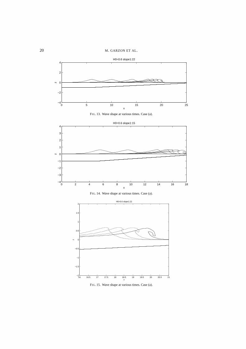
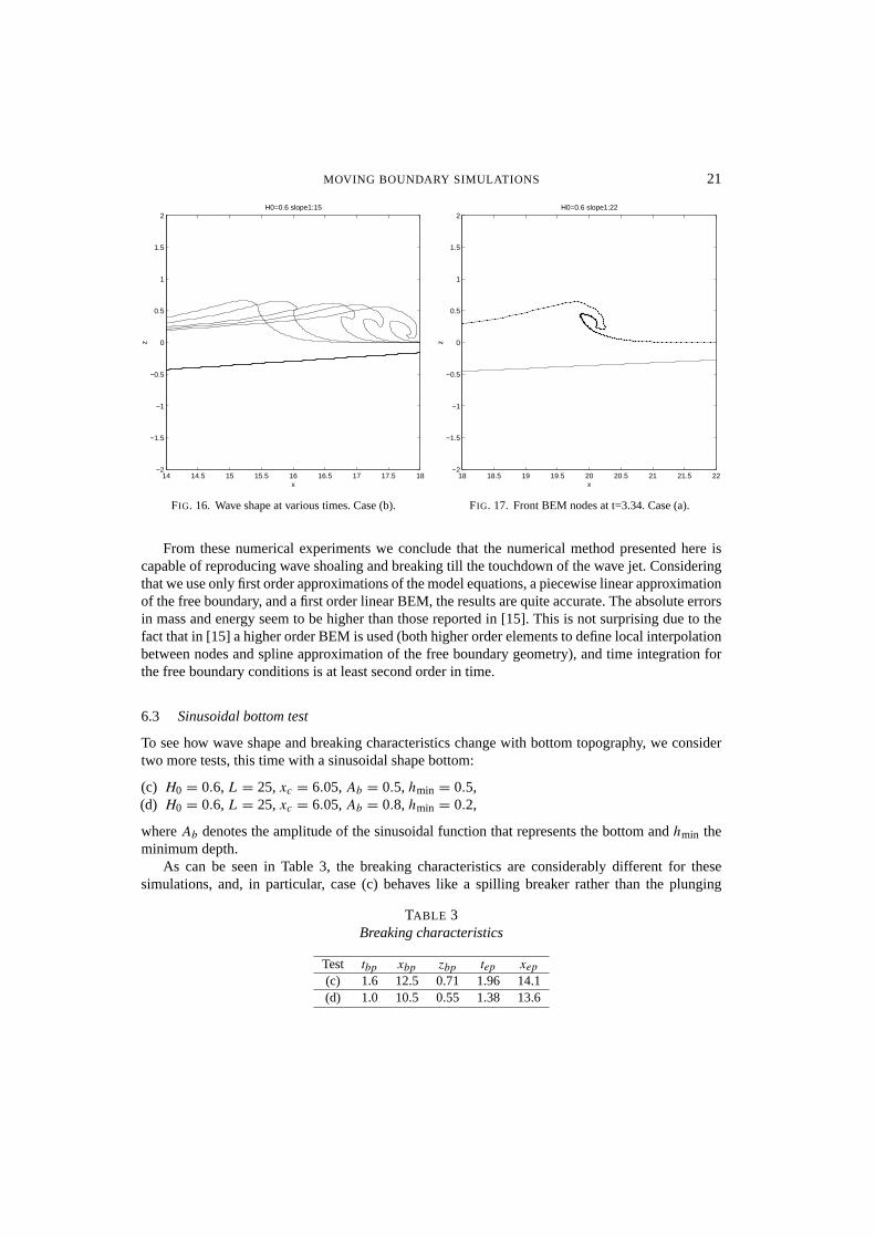
Figure 13 shows wave shape for case (a) att = 0,1,2,2.76,2.94,2.14,3.34 and Figure 14shows wave shape for case (b) att = 0,1,2,2.34,2,48,2.68,2.90. In Figures 15 and 16 we showin more detail the wave profiles from the BP to the EP for cases (a) and (b) respectively. Finally, inFigure 17 the front BEM nodes for case (a) and time 3.34 are shown.
20 M . GARZON ET AL.
0 5 10 15 20 25−4
−2
0
2
4H0=0.6 slope1:22
x
z
FIG. 13. Wave shape at various times. Case (a).
0 2 4 6 8 10 12 14 16 18−4
−3
−2
−1
0
1
2
3
4H0=0.6 slope1:15
x
z
FIG. 14. Wave shape at various times. Case (a).
16 16.5 17 17.5 18 18.5 19 19.5 20 20.5 21−2
−1.5
−1
−0.5
0
0.5
1
1.5
2H0=0.6 slope1:22
x
z
FIG. 15. Wave shape at various times. Case (a).
MOVING BOUNDARY SIMULATIONS 21
14 14.5 15 15.5 16 16.5 17 17.5 18−2
−1.5
−1
−0.5
0
0.5
1
1.5
2H0=0.6 slope1:15
x
z
FIG. 16. Wave shape at various times. Case (b).
18 18.5 19 19.5 20 20.5 21 21.5 22−2
−1.5
−1
−0.5
0
0.5
1
1.5
2H0=0.6 slope1:22
x
z
FIG. 17. Front BEM nodes at t=3.34. Case (a).
From these numerical experiments we conclude that the numerical method presented here iscapable of reproducing wave shoaling and breaking till the touchdown of the wave jet. Consideringthat we use only first order approximations of the model equations, a piecewise linear approximationof the free boundary, and a first order linear BEM, the results are quite accurate. The absolute errorsin mass and energy seem to be higher than those reported in [15]. This is not surprising due to thefact that in [15] a higher order BEM is used (both higher order elements to define local interpolationbetween nodes and spline approximation of the free boundary geometry), and time integration forthe free boundary conditions is at least second order in time.
6.3 Sinusoidal bottom test
To see how wave shape and breaking characteristics change with bottom topography, we considertwo more tests, this time with a sinusoidal shape bottom:
(c) H0 = 0.6,L = 25,xc = 6.05,Ab = 0.5,hmin = 0.5,(d) H0 = 0.6,L = 25,xc = 6.05,Ab = 0.8,hmin = 0.2,
whereAb denotes the amplitude of the sinusoidal function that represents the bottom andhmin theminimum depth.
As can be seen in Table 3, the breaking characteristics are considerably different for thesesimulations, and, in particular, case (c) behaves like a spilling breaker rather than the plunging
TABLE 3Breaking characteristics
Test tbp xbp zbp tep xep
(c) 1.6 12.5 0.71 1.96 14.1(d) 1.0 10.5 0.55 1.38 13.6

22 M . GARZON ET AL.
2 4 6 8 10 12 14 16 18 20−4
−3
−2
−1
0
1
2
3
4H0=0.6 , sinusoidal bottom
x
z
FIG. 18. Wave shape at various times. Case (c).
2 4 6 8 10 12 14 16 18 20−4
−3
−2
−1
0
1
2
3
4H0=0.6 , sinusoidal bottom
x
z
FIG. 19. Wave shape at various times. Case (d).
0 0.2 0.4 0.6 0.8 1 1.2 1.4 1.6 1.8 2
1.88
1.9
1.92
1.94
1.96
1.98
2Wave mass
time
mas
s
(c)(d)
FIG. 20. Wave mass vs time. Case (c) and (d).
MOVING BOUNDARY SIMULATIONS 23
0 0.2 0.4 0.6 0.8 1 1.2 1.4 1.6 1.8 20.2
0.3
0.4
0.5
0.6
0.7
0.8
0.9Wave Energy
time
E
EpEkE
FIG. 21. Wave energy. Case (c).
0 0.2 0.4 0.6 0.8 1 1.2 1.40.25
0.3
0.35
0.4
0.45
0.5
0.55
0.6
0.65
0.7
0.75Wave Energy
time
E
EpEkE
FIG. 22. Wave energy. Case (d).
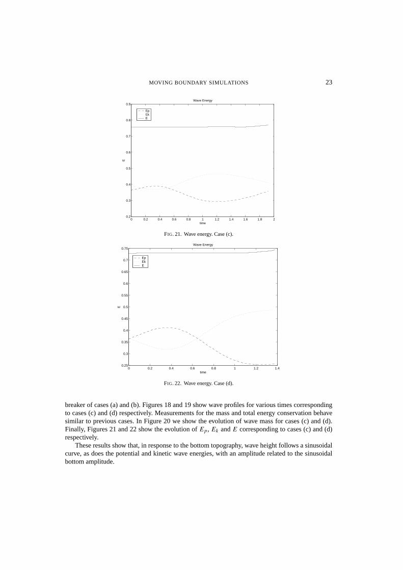
breaker of cases (a) and (b). Figures 18 and 19 show wave profiles for various times correspondingto cases (c) and (d) respectively. Measurements for the mass and total energy conservation behavesimilar to previous cases. In Figure 20 we show the evolution of wave mass for cases (c) and (d).Finally, Figures 21 and 22 show the evolution ofEp, Ek andE corresponding to cases (c) and (d)respectively.
These results show that, in response to the bottom topography, wave height follows a sinusoidalcurve, as does the potential and kinetic wave energies, with an amplitude related to the sinusoidalbottom amplitude.
24 M . GARZON ET AL.
6.4 Accuracy comments
The accuracy in our calculations is essentially first order. To recall our procedure, we first obtainthe level set nodes in the front, and we then find the zero level set using linear interpolation frommesh values. The velocity potential is bicubically interpolated from the mesh onto BEM nodes, andthen the velocity components at level set nodes are obtained by linear interpolation from velocitiescomputed on BEM nodes. We note that we do not see a decrease in error with decreasing time step,most probably because interpolation errors play a dominant role. Only the velocity potential errordecreases with decreasing time step, and this is probably due to the bicubic interpolation of thisvariable.
Additionally, we have used a first order boundary element method in these simulations. Indeed,we later implemented a second order version in both space and time for the level set update and forthe update of the potentialG equation. However, our results show that this additional accuracy wasovershadowed by the error in the boundary element solver. We have recently built a cubic Hermitesecond order method, which is now being incorporated into our electrospray simulations, and wewill report on this work elsewhere.
To summarize, we have built a coupled level set–boundary element algorithm for modelinga class of free boundary problems, in particular, two-dimensional breaking waves over slopingbeaches. The algorithm rests on a fully nonlinear potential model for a single fluid with appropriateboundary conditions, with both the interface location and the velocity potential recast as anembedded function throughout the domain. The use of a boundary integral method avoids far-fieldboundary conditions for the air, and the use of a level set method avoids complex gridding. Theformulation is unchanged in three dimensions; we shall report elsewhere on the extension of thisapproach to three-dimensional flow, as well as introduce a new model for what happens when thebreaking wave reconnects with the surface.
Acknowledgments
All work was performed at the Lawrence Berkeley National Laboratory, and the MathematicsDepartment of the University of California at Berkeley. The authors would like to thank S. T.Grilli for the use of an initialization computer code of Tanaka’s method, and for helpful comments.The first author was partially supported by the Spanish DGI Project BFM 00-1324 and would liketo thank Nilo Bobillo and Omar Menendez for their valuable collaboration. The third author wassupported by the Applied Mathematical Sciences Research Program of the Office of Mathematical,Information, and Computational Sciences, U.S. Department of Energy, under contract DE-AC05-00OR22725 with UT-Battelle, LLC.
REFERENCES
1. ADALSTEINSSON, D. & SETHIAN , J. A. A fast level set method for propagating interfaces.J. Comput.Phys.118(1995), 269–277. Zbl 0823.65137 MR 1329634
2. ADALSTEINSSON, D. & SETHIAN , J. A. The fast construction of extension velocities in level setmethods.J. Comput. Phys.148(1999), 2–22. Zbl 0919.65074 MR 1665209
3. ADALSTEINSSON, D. & SETHIAN , J. A. Transport and diffusion of material quantities on propagatinginterfaces via level set methods.J. Comput. Phys.185(2002), 271–288. Zbl 1047.76093 MR 2010161
MOVING BOUNDARY SIMULATIONS 25
4. BEALE, J. T., HOU, T. Y., & L OWENGRUB, J. Convergence of a boundary integral method for waterwaves.SIAM J. Numer. Anal.33 (1996), 1797–1843. Zbl 0858.76046 MR 1411850
5. BONNET, M. Boundary Integral Equation Methods for Solids and Fluids. Wiley (1995). Zbl 0920.730016. BREBBIA, C. A., TELLES, J. C. F., & WROBEL, L. C. Boundary Element Techniques. Springer (1984).
Zbl 0556.73086 MR 09349227. CHEN, S., MERRIMAN, B., OSHER, S., & SMEREKA, P. A simple level set method for solving Stefan
problems.J. Comput. Phys.135(1997), 8–29. Zbl 0889.65133 MR 14617058. CHANG, Y. C., HOU, T. Y., MERRIMAN, B., & OSHER, S. J. A level set formulation of Eulerian
interface capturing methods for incompressible fluid flows.J. Comput. Phys.124 (1996), 449–64.Zbl 0847.76048 MR 1383769
9. CHOPP, D. L. Some improvements of the fast marching method.SIAM J. Sci. Comput.23 (2001), 230–244. Zbl 0991.65105 MR 1860913
10. CHORIN, A. J. Numerical solution of the Navier–Stokes equations.Math. Comp.22 (1968), 745–762.Zbl 0198.50103 MR 0242392
11. CHRISTENSEN, E. D. & DEIGAARD, R. Large eddy simulation of breaking waves.Coastal Engrg.42(2001). 53–86.
12. EGGERS, J. Nonlinear dynamics and breakup of free-surface flows.Rev. Mod. Phys.69 (1997), 865–929.13. GRAY, L. J. Evaluation of singular and hypersingular Galerkin boundary integrals: direct limits and
symbolic computation.Singular Integrals in the Boundary Element Method, V. Sladek and J. Sladek (eds.),Computational Mechanics Publ. (1998), Chapter 2, 33–84.
14. GRAY, L. J., PHAN , A. -V. & K APLAN , T. Boundary integral evaluation of surface derivatives.SIAM J.Sci. Comput.26 (2004), 294–312. Zbl pre02138744 MR 2114345
15. GRILLI , S. T., GUYENNE, P., & DIAS, F. A fully non-linear model for three dimensional overturningwaves over an arbitrary bottom.Internat. J. Numer. Methods Fluids35 (2001), 829–867. Zbl 1039.76043
16. GRILLI , S. T., SVENDSEN, I. A., & SUBRAMANYA , R. Breaking criterion and characteristics forsolitary waves on slopes.J. Waterway, Port, Coastal, and Ocean Engrg.(June 1997).
17. GRILLI , S. T. Modeling of non-linear wave motion in shallow water.Computational Methods for Freeand Moving Boundary Problems in Heat and Fluid Flow, L. C. Wrobel and C. A. Brebbia (eds.),Computational Mechanics Publ., Southampton (1995), 91–122.
18. GRILLI , S. T. & SUBRAMANYA , R. Numerical modeling of wave breaking induced by fixed or movingboundaries.Comput. Mech.17 (1996), 374–391. Zbl 0851.76043 MR 1395439
19. LIN , P., CHANG, K., & L IU , P. L. Runup and rundown of solitary waves on sloping beaches.J. Waterway, Port, Coastal, and Ocean Engrg.(Sep/Oct 1999).
20. MALLADI , R., SETHIAN , J. A., & VEMURI, B. C. Shape modeling with front propagation: a level setapproach.IEEE Trans. Pattern Anal. Machine Intelligence17 (1995), 158–175.
21. MARTIN , P. A., RIZZO, F. J., & CRUSE, T. A. Smoothness-relaxation strategies for singular andhypersingular integral equations.Internat. J. Numer. Meth. Engrg.42 (1998), 885–906. Zbl 0913.65105MR 1630300
22. MARTIN , P. A. & RIZZO, F. J. On boundary integral equations for crack problems.Proc. Roy. Soc.LondonA421 (1989), 341–355. Zbl 0674.73071 MR 0985268
23. MARTIN , P. A. & RIZZO, F. J. Hypersingular integrals: how smooth must the density be?Internat.J. Numer. Meth. Engrg.39 (1996), 687–704. Zbl 0846.65070 MR 1377122
24. NOTZ, P. K. & BASARAN, O. A. Dynamics of drop formation in an electric field.J. Colloid InterfaceSci.213(1999), 218–237.
25. OSHER, S. & SETHIAN , J. A. Fronts propagating with curvature-dependent speed: algorithms based onHamilton–Jacobi formulations.J. Comput. Phys.79 (1988), 12–49. Zbl 0659.65132 MR 0965860
26. PEREGRINE, D. H. Breaking waves on beaches.Ann. Rev. Fluid Mech.15 (1983), 149–178.
26 M . GARZON ET AL.
27. SETHIAN , J. A. An analysis of flame propagation. Ph.D. Dissertation, Dept. of Mathematics, Univ. ofCalifornia, Berkeley, CA (1982).
28. SETHIAN , J. A. Curvature and the evolution of fronts.Comm. Math. Phys.101 (1985), 487–499.Zbl 0619.76087 MR 0815197
29. SETHIAN , J. A. Numerical methods for propagating fronts.Variational Methods for Free SurfaceInterfaces, P. Concus and R. Finn (eds.), Springer (1987), 155–164. Zbl 0618.65128 MR 0872900
30. SETHIAN , J. A. A fast marching level set method for monotonically advancing fronts.Proc. Nat. Acad.Sci. U.S.A.93 (1996), 1591–1595. Zbl 0852.65055 MR 1374010
31. SETHIAN , J. A. Level Set Methods and Fast Marching Methods.Cambridge Monogr. Appl. Comput.Math., Cambridge Univ. Press (1999). Zbl 0973.76003 MR 1700751
32. SETHIAN , J. A. & SMEREKA, P. Level set methods for fluid interfaces.Ann. Rev. Fluid Mech.35 (2003),341–372. Zbl 1041.76057 MR 1967017
33. SETHIAN , J. A. & STRAIN , J. D. Crystal growth and dendritic solidification.J. Comput. Phys.98(1992),231–253. Zbl 0752.65088 MR 1150905
34. SUSSMAN, M., SMEREKA, P., & OSHER, S. J. A level set approach to computing solutions toincompressible two-phase flow.J. Comput. Phys.114(1994), 146–159. Zbl 0808.76077
35. TANAKA , M. The stability of solitary waves.Phys. Fluids29 (1986), 650–655. Zbl 0605.76025MR 0828181
36. YAN , F., FAROUK, B., & KO, F. Numerical modeling of an electrostatically driven liquid meniscus inthe cone-jet mode.Aerosol Sci.34 (2003), 99–116.
37. YU, J.-D., SAKAI , S., & SETHIAN , J. A. A coupled level set projection method applied to ink jetsimulation.Interfaces Free Bound.5 (2003), 459–482. Zbl 1042.35059 MR 2031466
38. ZELT, J. A. The run-up of non-breaking and breaking solitary waves.Coastal Engrg.15(1991), 205–246.39. ZHU, J. & SETHIAN , J. A. Projection methods coupled to level set interface techniques.J. Comput. Phys.
102(1992), 128–138. Zbl 0751.76050