theoretical and experimental investigation of a ... · the commercial software trnsys and the solar...

SIMULATIONS OF A LARGE SCALE SOLAR THERMAL POWER PLANT

IN TURKEY

USING CONCENTRATING PARABOLIC TROUGH COLLECTORS

A THESIS SUBMITTED TO

THE GRADUATE SCHOOL OF NATURAL AND APPLIED SCIENCES

OF

MIDDLE EAST TECHNICAL UNIVERSITY

BY

YASEMİN USTA

IN PARTIAL FULFILLMENT OF THE REQUIREMENTS

FOR

THE DEGREE OF MASTER OF SCIENCE

IN

MECHANICAL ENGINEERING

DECEMBER 2010

Approval of the thesis:


IN TURKEY USING CONCENTRATING PARABOLIC TROUGH

COLLECTORS

submitted by YASEMİN USTA in partial fulfillment of the requirements for the

degree of Master of Science in Mechanical Engineering Department, Middle

East Technical University by,

Prof. Dr. Canan Özgen

Dean, Graduate School of Natural and Applied Sciences

Prof.Dr. Suha Oral

Head of Department, Mechanical Engineering

Associate Prof. Dr. Derek K. Baker

Supervisor,Mechanical Engineering Dept., METU

Prof. Dr. Bilgin Kaftanoğlu

Co-sup., Manufacturing Eng., Dept., Atılım Uni.

Examining Committee Members:

Associate Prof. Dr. Derek K. Baker

Mechanical Engineering Dept., METU

Prof. Dr. Bilgin Kaftanoğlu

Manufacturing Engineering Dept., Atılım University

Assoc. Prof. Dr.Cemil Yamalı


Assistant Prof. Dr. Tuba Okutucu Özyurt


Assoc. Prof. Dr. Nilay Sezer Uzol

Mechanical Engineering Dept.,

TOBB University of Economics and Technology

Date:

iii

I hereby declare that all information in this document has been obtained and

presented in accordance with academic rules and ethical conduct. I also declare

that, as required by these rules and conduct, I have fully cited and referenced

all material and results that are not original to this work.

Name, Last name: Yasemin Usta

Signature :

iv

ABSTRACT


IN TURKEY

USING CONCENTRATING PARABOLIC TROUGH COLLECTORS

Usta,Yasemin

M.Sc., Department of Mechanical Engineering

Supervisor: Assoc. Prof. Dr. Derek K. Baker

Co-Supervisor: Prof. Dr. Bilgin Kaftanoğlu

December 2010, 130 Pages

In this study, the theoretical performance of a concentrating solar thermal electric

system (CSTES) using a field of parabolic trough collectors (PTC) is investigated.

The commercial software TRNSYS and the Solar Thermal Electric Components

(STEC) library are used to model the overall system design and for simulations. The

model was constructed using data from the literature for an existing 30-MW solar

electric generating system (SEGS VI) using PTC’s in Kramer Junction, California.

The CSTES consists of a PTC loop that drives a Rankine cycle with superheat and

reheat, 2-stage high and 5-stage low pressure turbines, 5-feedwater heaters and a

dearator. As a first approximation, the model did not include significant storage or

back-up heating. The model’s predictions were benchmarked against published data

for the system in California for a summer day. Good agreement between the model’s

predictions and published data were found, with errors usually less than 10%. Annual

simulations were run using weather data for both California and Antalya, Turkey.

The monthly outputs for the system in California and Antalya are compared both in

terms of absolute monthly outputs and in terms of ratios of minimum to maximum

monthly outputs. The system in Antalya is found to produce30 % less energy

v

annually than the system in California. The ratio of the minimum (December) to

maximum (July) monthly energy produced in Antalya is 0.04.

Keywords: Concentrating solar, thermal power, parabolic trough collector,

simulation.

vi

ÖZ

TÜRKİYE’DE BÜYÜK ÖLÇEKLİ GÜNEŞ ENERJİSİ SİSTEMLERİNİN

PARABOLİK OLUKLU KOLLEKTÖRLER KULLANILARAK SİMÜLASYONU

Usta,Yasemin

Yüksek Lisans, Makina Mühendisliği Bölümü

Tez Yöneticisi : Doç. Dr. Derek K. Baker

Ortak Tez Yöneticisi: Prof. Dr. Bilgin Kaftanoğlu

Aralık 2010, 130 Sayfa

Bu çalışmada parabolik oluklu kolektörler kullanılarak yoğunlaştırılmış güneş

enerjisi sistemlerinin teorik performansı incelenmiştir. Sistemin tümünün tasarımında

ve simülasyonunda TRNSYS yazılımı ve ona bağlı STEC kütüphanesi kullanılmıştır.

Kaliforniya Kramer Junction’da güneş enerjisi ile 30 MW değerinde elektrik üretimi

yapan sistem örnek alınmıştır. Sistem parabolik oluklu kollektörler ve buna bağlı

ısıtıcı ve ön ısıtıcı, beş adet besleme suyu ısıtıcısı yüksek basınç ve alçak basınç

türbinlerini ve bir adet açık çevrim ısıtıcısı ile Rankine çevrimini oluşturmaktadır.

Ilk olarak sistemde bir depolama yada ek ısıtma sistemi kullanılmamıştır.Sistemin

yaz ayları için elde edilmiş sonuçları Kaliforniya’daki sistem sonuçları ile

karşılaştırılmıştır. Sonuçlar karşılaştırıldığında %10 dan daha az hata görülmüştür.

Kaliforniya ve Antalya’nın koşulları uygulanarak sistem bir yıl için simüle edildi.

Kaliforniya ve Antalya’nın aylık verileri minimum ve maksimum oranları

karşılaştırıldı. Antalya’da kurulan sistemin yıllık toplamda %30 daha az enerji

ürettiği belirlenmiştir. Antalya’nın aralık ayındaki minimum enerjisinin maksimum

enerjisine oranı 0.04 olarak bulunmuştur.

vii

Anahtar Kelimeler: Yoğunlaştırılmış güneş enerjisi, parabolic oluklu kolektörler, ve

simulasyonu.

viii

To my husband and my family

ix

ACKNOWLEDGEMENTS

I am deeply grateful to my supervisor, Assoc. Prof. Derek K. Baker, for his

perceptive supervision, everlasting support and encouragement.

I also would like to thank my co-supervisor Prof. Dr. Bilgin Kaftanoğlu.

I appreciate his guidance, leadership and advices.

I would also thank to jury members for their comments.

Finally, I would like to express my deepest feelings to my husband and parents for

their continuous encouragement, understanding, and support.

x

TABLE OF CONTENTS

ABSTRACT……………...…………...……………………………………………..... iv

ÖZ……………………………………….…….………………………………………..vi

ACKNOWLEDMENTS……………………..…………………….…………………...ix

TABLE OF CONTENTS ................................................................................................. x

LIST OF TABLES ........................................................................................................ xii

LIST OF FIGURES ....................................................................................................... xv

LIST OF SYMBOLS ................................................................................................. xviii

CHAPTERS ..................................................................................................................... 1

1.INTRODUCTION ........................................................................................................ 1

1.1. Background Information ......................................................................................... 1

1.2. Current Solar-Thermal Power Situation.................................................................. 3

2. SURVEY OF LITERATURE AND OBJECTIVES .................................................... 8

2.1 Overview of Solar Thermal Energy Generating Systems ........................................ 8

2.2 Sun-Earth Geometric Relations ............................................................................... 9

2.3 Solar Radiation ....................................................................................................... 13

2.4. Previous Modeling and Simulation Studies .......................................................... 15

2.5. Objectives of Current Work .................................................................................. 17

3. MODELS ................................................................................................................... 18

3.1. The Plant Model .................................................................................................... 18

3.2. Power Cycle Model ............................................................................................... 24

3.3. Flow and Temperature – Entropy Diagrams ......................................................... 25

3.4. TRNSYS and STEC Library ................................................................................. 27

3.5. Superheater ............................................................................................................ 31

3.6. Boiler (Steam Generator) ...................................................................................... 34

3.7. Preheater ................................................................................................................ 36

xi

3.8. High Pressure and Low Pressure Turbine ............................................................. 38

3.9. Reheater................................................................................................................. 43

3.10. Low Pressure (LP) Turbine ................................................................................. 45

3.11. Condenser ............................................................................................................ 49

3.12. Pump .................................................................................................................. 52

3.13. Deaerator ............................................................................................................. 55

3.14. Feedwater heaters ............................................................................................... 57

3.15. Weather data........................................................................................................ 63

3.16. Expansion vessel ................................................................................................ 64

3.17. Parabolic Trough Field ....................................................................................... 66

3.18. Model Capabilities and Limitations .................................................................... 69

4. RESULTS .................................................................................................................. 71

4.1 Model Validation ................................................................................................... 71

4.2 Antalya’s Results ................................................................................................... 75

5. SUMMARY AND CONCLUSIONS ........................................................................ 83

6. SUGGESTIONS FOR FUTURE INVESTIGATIONS ............................................. 85

REFERENCES ............................................................................................................... 87

APPENDICES ............................................................................................................... 92

A.PARABOLIC TROUGH COLLECTOR DESIGN TOOL USING VISUAL

BASIC………………………………………………………………………………..92

B. TMY2 DATA AND FORMAT ............................................................................... 99

C. SAMPLE TRNSYS INPUT (DECK) FILE…………..………………………….103

xii

LIST OF TABLES

TABLES

Table 2.1 Characteristics of SEGS plants at Kramer Junction .......................................... 8

Table 3.1 Description of Connections…………………………………………………..31

Table 3.2 Constant Parameters and Initial Conditions for Superheater ........................... 32

Table 3.3 Input Links for the Superheater ....................................................................... 33

Table 3.4 Output Links for the Superheater ..................................................................... 33

Table 3.5 Constant Parameters and Initial Conditions for Boiler .................................... 35

Table 3.6 Input Links for the Boiler................................................................................. 35

Table 3.7 Output Links for the Boiler .............................................................................. 36

Table 3.8 Constant Parameters and Initial Conditions for Preheater ............................... 37

Table 3.9 Input Links for the Preheater ........................................................................... 38

Table 3.10 Output Links for the Preheater ....................................................................... 38

Table 3.11 Constant Parameters and Initial Conditions for HP turbine 1st stage ............ 41

Table 3.12 Initial Parameters for the HP Turbine 1st stage splitter ................................. 41

Table 3.13 Constant Parameters and Initial Conditions for HP Turbine 2nd Stage ........ 42

Table 3.14 Input and Output Links for the Turbine Stage ............................................... 43

Table 3.15 Initial Parameters for the HP Turbine 2nd Stage Splitter .............................. 43

Table 3.16 Constant Parameters and Initial Conditions for the Reheater ........................ 44

Table 3.17 Input Links for the Reheater .......................................................................... 44

Table 3.18 Output Links for the Reheater ........................................................................ 45

Table 3.19 Initial Conditions and Constants for LP turbine 1st stage ............................. 46

Table 3.20 Initial parameters for LP turbine 1st stage splitter ......................................... 46

Table 3.21 Initial Conditions and Constants for LP turbine 2st stage ............................. 46

Table 3.22 Initial Parameters for LP Turbine 2nd Stage Splitter ..................................... 47

Table 3.23 Initial Conditions and Constants for LP Turbine 3rd Stage ........................... 47

xiii

Table 3.24 Initial Parameters for LP Turbine 3rd Stage Splitter ..................................... 47

Table 3.25 Initial Conditions and Constants for LP Turbine 4rd Stage ........................... 48

Table 3.26 Initial Parameters for LP Turbine 4rd Stage Splitter ..................................... 48

Table 3.27 Initial Conditions and Constants for LP turbine 5th stage ............................. 49

Table 3.28 Initial Conditions and Constants for the Condenser ...................................... 51

Table 3.29 Input Links for the Condenser ....................................................................... 51

Table 3.30 Output Links for the Condenser ..................................................................... 52

Table 3.31 Initial Conditions and Constants for the Condensate Pump .......................... 53

Table 3.32 Input and Output Links for the Condensate Pump ......................................... 53

Table 3.33 Initial Conditions and Constants for the Feed Pump ..................................... 54

Table 3.34 Output and Input Links for Feedwater Pump................................................. 54

Table 3.35 Initial Conditions and Constants for the HTF Pump ..................................... 55

Table 3.36 Output and Input Links for HTF Pump .......................................................... 55

Table 3.37 Initial Conditions and Constants for the Dearator ......................................... 56

Table 3.38 Input Links for Dearator ................................................................................ 57

Table 3.39 Output Links for the Dearator ........................................................................ 57

Table 3.40 Initial Conditions and Constants for the 1st Feedwater Heater (FWH1) ....... 59

Table 3.41 Input Links for Feedwater Heater1 ................................................................ 60

Table 3.42 Output Links for Feedwater Heater1 ............................................................. 60

Table 3.43 Initial Conditions and Constants for the 2nd Feedwater Heater (FWH2) ..... 61

Table 3.44 Initial Conditions and Constants for 3rd Feedwater Heater (FWH3) ............ 62

Table 3.45 Initial Conditions and Constants for 5th Feedwater Heater (FWH5) ............ 62

Table 3.46 Initial Conditions and Constants for the 6th Feedwater Heater (FWH6) ...... 63

Table 3.47 Initial Parameters for weather data file .......................................................... 64

Table 3.48 Input Links for Weather Data File ................................................................. 64

Table 3.49 Initial Parameters for expansion vessel .......................................................... 65

Table 3.50 Input Links for the Expansion Vessel ............................................................ 66

Table 3.51 Output Links for the Expansion Vessel ......................................................... 66

Table 3.52 Thermal Performance coefficients ................................................................ 67

xiv

Table 3.53 Initial Conditions and Constants for the Parabolic Trough Collector ............ 68

Table 3.54 Input Links for the Trough ............................................................................. 69

Table 3.55 Output Links for the Trough .......................................................................... 69

Table B. 1 Header Elements in the TMY2 Format…………………………………....101

Table B. 2 Data Elements in the TMY2 Format ............................................................ 101

xv

LIST OF FIGURES

FIGURES

Figure 1.1 Diagram of Basic Solar Energy Conversion Systems ..................................... 2

Figure 1.2 Areas of the World with High Insolation ........................................................ 3

Figure 1.3 Power Tower System ....................................................................................... 4

Figure 1.4 Parabolic Dish Collector .................................................................................. 5

Figure 1.5 Parabolic Trough Collector Field .................................................................... 6

Figure 2.1 Solar Collector Assembly…………………………………………………...9

Figure 2.2 Angle of Incidence on a Parabolic Trough Collector .................................... 10

Figure 2.3 Declination Angle due to the Earth ............................................................... 10

Figure 2.4 Solar Declination vs. day of year ................................................................... 11

Figure 2.5 Equation of time versus month of the year .................................................... 12

Figure 2.6 Collector tracking through morning, showing digression .............................. 15

Figure 3.1 Layout of the SEGS VI Solar trough Field KJC Operating Company… …..18

Figure 3.2 Part of the Parabolic Trough Collector ........................................................... 19

Figure 3.3 Schematic of a Solar Collector Assembly ...................................................... 20

Figure 3.4 LS-3 space frame, EuroTrough torque-box, and Duke Solar Space Frame

concentrator designs ........................................................................................................ 21

Figure 3.5 Vacuum Tube ................................................................................................. 22

Figure 3.6 A photo of Vacuum Tube Connection ............................................................ 23

Figure 3.7 Flow Diagram of the SEGSVI Plant .............................................................. 24

Figure 3.8 Flow Diagram for Power Cycle -state points labelled .................................... 26

Figure 3.9 Temperature- Entropy Diagram of Power Cycle at Reference State ............. 27

Figure 3.10 The SEGS VI TRNSYS Model .................................................................... 28

Figure 3.11 Parameters Window ...................................................................................... 29

Figure 3.12 Sample Connection Window Showing Connection Between Weather Data30

xvi

Figure 3.13 Flow diagram of superheater ........................................................................ 32

Figure 3.14 Flow diagram of boiler (steam generator) .................................................... 34

Figure 3.15 Flow Diagram of Preheater ........................................................................... 37

Figure 3.16 Flow Diagram of Turbine Stage Consisting of a Turbine and a Splitter. ..... 39

Figure 3.17 STEC Components Turbine and Splitters .................................................... 40

Figure 3.18 STEC Components Turbine and Splitter ...................................................... 45

Figure 3.19 Flow Diagram of Condenser ......................................................................... 50

Figure 3.20 Flow Diagram of a Pump .............................................................................. 53

Figure 3.21 Flow Diagram of a Dearator ......................................................................... 56

Figure 3.22 Flow Diagram of a Feedwater Heater ........................................................... 58

Figure 3.23 Stec Component Feedwater Heater .............................................................. 59

Figure 3.24 Flow diagram of expansion vessel ................................................................ 65

Figure 4.1 Weather Conditions July 18, 1991…...……………………………………...71

Figure 4.2 Weather Conditions July 18, 1991 TRNSYS results ...................................... 72

Figure 4.3 Comparison of TRNSYS Results and Real data plant DNI July 18, 1991 ..... 73

Figure 4.4 Measured and Predicted Gross Power Output on July 18,1991 ..................... 74

Figure 4.5 Gross Power Output TRNSYS Result July 18, 1991 ..................................... 74

Figure 4.6 Comparision of Power Results on 18/07/1991 ............................................... 75

Figure 4.7 Weather Condition of Antalya on August 3, 2005 ......................................... 76

Figure 4.8 Predicted Gross Power Output for Antalya for August 3, 2005. .................... 77

Figure 4.9 Clear Summer Week Power Results(July, 4-10 2005) ................................... 78

Figure 4.10 Cloudy Week Power Output Results(October,18-24 2005) ......................... 78

Figure 4.11 Winter Week Power Output Result(January,21-28 2005) ............................ 79

Figure 4.12 Clear Summer Week Power Output and DNI (July, 4-10 2005) .................. 79

Figure 4.13 Winter Week Power Output and DNI (January,21-28 2005)………………77

Figure 4.14 System, Cycle, Collector Efficiency versus Time Antalya for August 3,

2005……………………………………………………………………………………..81

Figure 4.15 System, Cycle, Collector Efficiency versus Time Antalya for January 21,

2005……………………………………………………………………………………..81

xvii

Figure 4.16 Comparison of Monthly Performance of CSP System in Antalya, Turkey,

and Kramer Junction, California: Average Daily Power Output, Ratio of Average Daily

to to Maximum Average Daily Output, and Ratio of Output in Antalya to Kramer

Junction (KJ). ................................................................................................................... 82

Figure A.1 Designing Parameters of Parabolic Trough Collector Field………………..93

Figure A.2 Selection of City, Months and Coating of the Collector ............................... 94

Figure A.3 Result Window .............................................................................................. 95

Figure A.4 Error Message ................................................................................................ 96

Figure A.5 Vacuum Tube Datas....................................................................................... 97

Figure B. 1 Sample file header and data in the TMY2 format for January 1…………100

xviii

LIST OF SYMBOLS

C capacitance

E the equation of time [min]

h specific enthalpy(kJ kg-1

)

H enthalpy(kJ)

K incidence Angle Modifier

Lst standard meridian for the local time zone(deg)

Lloc the longtitude of the location (deg)

m mass (kg)

mass flowrate(kg h-1

)

n day number of the year

P pressure(bar)

Q heat transfer (kJ)

θz zenith angle (deg)

ω hour angle (deg)

T temperature(oC)

UA overall heat transfer factor(kJ h-1

K-1

)

mechanical power (MW)

ΔT temperature difference (K)

Greek Symbols

ϕ latitude

δ declination angle(deg)

ɛ effectiveness

isentropic efficiency

xix

Subscripts

htf heat transfer fluid

in inlet

max maximum

min minimum

REF reference

out outlet

Abbreviations

CSP concentrating solar power

DNI direct normal irradiance

FWH feedwater heater

HCE heat transfer element

HTF heat transfer fluid

HP high pressure

LP low pressure

NTU number of transfer units

PTC parabolic trough collector

SEGS solar energy generating systems

STEC solar thermal electric component

TMY typical meteorogical year

SCA solar collector area

1

CHAPTER I

INTRODUCTION

1.1. Background Information

Serious environmental problems and finite fossil resources result in the need for new

sustainable electricity generation options, which take advantage of renewable energies

and are economical. Solar energy has many benefits including environmental protection,

economic growth, job creation, and diversity of fuel supply. Solar energy technologies

can be deployed rapidly, and have the potential for global technology transfer and

innovation. The total (annual) solar energy striking the earth’s surface is 10,000 times

annual global energy consumption [1,2].

Solar energy has been used since B.C. for heating and mechanical applications. More

than two thousand years ago, in 212 B.C., Archimedes concentrated the sun’s rays using

mirrors. In 1615, a”solar powered motor” was invented by Salomon De Caux and was

the first recorded mechanical application of the Sun’s energy. Public institutions and

initiatives continue facilitate the development of solar conversion technologies and yield

an alternative to traditional energy sources, such as coal and oil [3].

Turkey is a developing country with an increasing energy demand. Solar resources and

large areas are widely available in the western and southeastern parts of Turkey. Solar

energy research in Turkey began in the 1960s as an alternative energy [4,5]. Water

heating has been used in Turkey since 1975 [6]. The Turkish government supports the

development of this technology strongly.

2

Solar resources can be converting into a useful form of energy by different types of solar

energy systems. Three of the most basic system types are shown as a block diagram in

Figure 1.1.

Figure 1.1 Diagram of basic solar energy conversion systems [7]

Heat for industrial process, water heating and house heating requires a thermal energy

source. Solar energy is used as a source to supply a thermal load. There are two

methods which are used to change solar energy into electricity. The first method is that

solar energy is collected as heat then changed into electricity using a traditional power

plant or heat engine. The second method is that solar energy is collected and converted

directly into electricity using photovoltaic cells [5,7].

As a result, solar energy is used for both industrial and residential purposes both

nationwide and worldwide. There is a strong need for advanced solar energy systems

3

that are environmental benign and more efficient so that solar energy systems can be

more competitive with traditional energy systems.

1.2. Current Solar-Thermal Power Situation

Solar energy is available over the entire globe. Some regions intercept more solar energy

than other regions because of the relative motion of the sun with respect to the earth and

variations in cloud cover. Solar energy conversion systems which are constructed in high

insolation areas are more efficient. Figure 1.2 shows high insolation areas and these

areas cover mainly desert zones and include many developing countries. The same

amount of heat or electricity can be obtained anywhere on the globe but in areas with

low insolation the size of the collectors needs to be increased. The amount, quality, and

timing of solar energy are the most important factors for solar energy system design [7].

Figure 1.2 Areas of the World with High Insolation [7]

Global solar irradiance is the total amount of solar radiation and includes both direct and

diffuse radiation. While non-concentrating solar energy conversion technologies can use

both direct and indirect radiation, concentrating solar energy conversion technologies

can only use direct irradiance.

http://www.3tier.com/en/support/glossary/#ghi

4

Concentrating solar power (CSP) herein refers specifically to solar thermal technologies

that obtain high temperature heat by concentrating solar energy. The sun’s energy is

converted to electric power using various concentrating mirror configurations. The

plants consist of two parts, one which are the collectors that concentrate sunlight to heat

a heat transfer fluid to a high temperature and the other which converts the thermal

energy in the hot heat transfer fluid to electricity.

Producing electricity from solar thermal technologies requires four main elements: 1)

concentrator; 2) receiver, 3) heat transfer fluid; and 4) power conversion system. The

three most common collector types for CSP are power towers, dish, and parabolic trough

collectors (PTC).

Solar power towers consist of “heliostat” mirrors that generate electric power from

sunlight by focusing concentrated solar radiation on a tower-mounted heat exchanger

(receiver). These plants have a 30 to 400 MW capacity for utility-scale applications

[1,3,7,8].Figure 1.3 shows a photo of a power tower system.

Figure 1.3 Power Tower System [9]

5

Parabolic Dish Collectors (or dish engine systems) consist of “dish parabolic-shaped”

mirrors used as a reflector. These mirrors concentrate and focus the sun’s rays onto a

receiver which is mounted at the focal point. These systems firstly convert the thermal

energy to mechanical energy then to electrical energy. Dish/engine systems are different

from other conventional solar thermal energy technologies as they do not use a heat

transfer fluid loop to connect the collector to the heat engine. Their concentrators are

mounted on a structure with a two-axis tracking system to follow the sun. The collected

heat is typically utilized directly by a heat engine mounted on the receiver moving with

the dish structure. 25 kW of electricity can be generated from each individual system.

The capacity can easily be increased by connecting dishes together [1,3,7,9,10]. Figure

1.4 shows a photo of parabolic dish collector.

Figure 1.4 Parabolic Dish Collector [9]

Parabolic Trough Collectors (PTC) consists of rows of trough-shaped mirrors which

concentrate solar insolation to a receiver tube placed along the focal axis of each trough.

The solar field is composed of many troughs which are placed in parallel rows. The

6

troughs are aligned along a north-south axis and track the sun from east to west during

the day. The focused radiation raises the temperature of the heat-transfer fluid, which is

used to generate steam.

The steam is then used to power a turbine-generator to produce electricity [1,3,5,7,11].

Figure 1.5 shows a photo of parabolic trough collector field.

Figure 1.5 Parabolic Trough Collector Field [9]

Concentrating solar thermal systems can be used for a wide range of different

applications including electricity production and heating. Different systems can produce

different temperatures. The maximum temperature scales with the system’s

concentration factor (C), defined as the ratio of the aperture area to the absorber area.

Parabolic trough, parabolic dish and power tower technologies can reach maximum

7

temperatures of 400 0C, 750

0C, and 1000

0C respectively. Additionally, PTC’s are also

appropriate for delivering process heat and driving thermally powered cooling cycles.

Both the dish and tower systems use 2-axis tracking while the PTC uses single axis

tracking. Of the three, only PTC’s have been commercialized with an installed capacity

of 354 MW, which are the LUZ plants built from 1984 to 1991 in California. Solar

towers and dish engines have been tested in a series of demonstration projects. For all

three types hybrid operation where a fossil fuel is used as a secondary energy source is

possible [1].

These technologies need further research to overcome non-technical and technical

barriers. The main non-technical barriers are financial or legal and include grid access,

financing, obtaining permits to build and operate, approval of environmental impact

assessments, and power purchase agreements.

Concentrating solar power technologies are more appropriate for plant sizes of 10 MW

electric or larger. These technologies offer the lowest –cost solar electricity. Recent

technologies cost $3 per watt and 12¢ per kilowatt-hour (kWh) of solar power. Hybrid

systems, which are a combination of concentrating solar power plants with coal plants or

natural gas combined cycles, can reduce costs to $1.5 per watt [12].

Turkey is a developing country with an increasing energy demand. Over the period of

1975-2008 the average electricity demand increased annually by 8.3% [13]. About 81%

of the electricity demand of Turkey in 2007 was met by coal, lignite, fuel oil, or LPG.

Natural gas, which is imported from neighboring countries, is about 61.2% [14]. About

19% of the electricity is supplied from wind and geothermal, etc. In 2016-2017

electricity demand in Turkey is predicted to exceed the supply [15].

8

CHAPTER 2

SURVEY OF LITERATURE AND OBJECTIVES

2.1 Overview of Solar Thermal Energy Generating Systems

Solar Energy Generating Systems (SEGS) I through IX parabolic trough plants were

built in the Mojave Desert in southern California between 1985 and 1991. The systems

have a total capacity of 354 MW. The first two systems are rated at 14MW and 30MW,

Systems III through VII are rated at 30MW each, and the final two SEGS plants are

rated at 80MW each. Luz International Company designed, built, and sold the nine

SEGS plants and as of 2006 these plants have performed well over their first 20 to 25

years of operation. Other parabolic trough collector projects are also planned and some

of them are active, including a 64 MW plant in Nevada and 50 MW plants in Spain [16].

Basic characteristics of the SEGS (III,IV,V,VI,VII) plants at the Kramer Junction site

are listed in Table 2.1.

Table 2.1 Characteristics of SEGS plants at Kramer Junction [16]

9

Figure 2.1 Solar Collector Assembly

Several long parallel rows of collectors comprise a solar field assembly ( (Figure 2.1).

The trough parts of the collectors are curved glass mirrors that focus direct radiation

from the sun onto a heat collection element. These collectors track the sun by rotating

around a north-south axis. The troughs concentration ratio is 71:1 for LS-2 and 80:1 for

LS-3 [11].

2.2 Sun-Earth Geometric Relations

The angles between the sun and a horizontal plane relative to the earth describe

important solar geometric relationships [17]. The angle of incidence (θ) in Figure 2.2

shows the angle between beam (also called direct) radiation and the normal to that

surface. The angle of incidence describes the position of the sun in the sky relative to a

10

surface. Throughout the day and year the angle of incidence will vary and the

performance of the collectors will be affected.

Figure 2.2 Angle of Incidence on a Parabolic Trough Collector [16]

The declination angle (δ), shown in Figure 2.3, shows the angular position of the sun at

solar noon with respect to the plane of the equator. The declination angle will change

throughout the year over a range of -23.45° ≤ δ ≤ 23.45°.

Figure 2.3 Declination Angle due to the Earth [16]

11

The following expression for declination angle was developed by P.I. Cooper in 1969

[17]

(2.1)

Here n is the day number of the year and varies from 1 (corresponding to January 1) to

365 (corresponding to December 31). Figure 2.4 shows the variation of the declination

angle throughout the year.

Figure 2.4 Solar Declination vs. day of year from Equation 2.1

Two types of times are used in solar engineering: solar time and standard time. Solar

time is measured with respect to the sun’s position. When the center of the sun is on an

observer's meridian (at its highest point during the day), the observer's local solar time is

zero and it is solar noon. However, standard time is based on a standard meridian for a

time zone that may lie to the east or west of the local meridian. Standard time is also

called “clock time” as it is the time shown on a common clock [17,18]. The difference in

minutes between solar time and standard time is

12

Solar time- Standart time= 4 (Lst-Lloc) + E (2.2)

where;

Lst = Standard meridian for the local time zone[deg]

Lloc = The longtitude of the location [deg]

E = The equation of time [min]

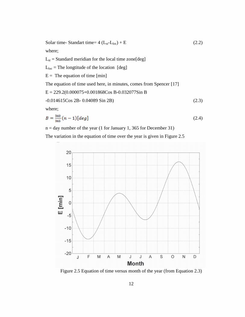
The equation of time used here, in minutes, comes from Spencer [17]

E = 229.2(0.000075+0.001868Cos B-0.032077Sin B

-0.014615Cos 2B- 0.04089 Sin 2B) (2.3)

where;

(2.4)

n = day number of the year (1 for January 1, 365 for December 31)

The variation in the equation of time over the year is given in Figure 2.5

Figure 2.5 Equation of time versus month of the year (from Equation 2.3)

13

The zenith angle (θz) is the angle between the vertical and the line to the sun. The zenith

angle is related to both the declination angle and the hour angle by the following

relationship [17].

Cos θz = Cos (δ) Cos (ϕ) Cos (ω) + Sin (δ) Sin (ϕ) (2.5)

δ = declination angle (see Equation 2.1)

ω = hour angle (see Equation 2.6)

ϕ = latitude

The hour angle is the angular displacement of the sun east or west from the local

meridian at noon local time. This angle is related to the earth’s rate of rotation on its axis

of 15° per hour. At solar noon, the hour angle is zero and the sun is in line with the local

meridian on earth. The hour angle is negative before solar noon when the sun is east of

the local meridian and positive after solar noon when the sun is west of the local

meridian [17,18].

(2.6)

where ω is the hour angle [deg] and SolarTime is the solar time [hr].

2.3 Solar Radiation

The radiation reaching the earth's surface can be represented in a number of different

ways. Global Horizontal Irradiance is the total amount of shortwave radiation which

includes both Direct Normal Irradiance (DNI, also called beam normal) and Diffuse

Horizontal Irradiance Global Horizontal Irradiance is the radiation received by a surface

horizontal to the ground.

Direct Normal Irradiance is the amount of solar radiation that has not been scattered or

absorbed by the atmosphere received per unit area by a surface normal to the sun-earth

line.

http://www.3tier.com/en/support/glossary/#ghi

14

Diffuse Horizontal Irradiance is the amount of radiation received per unit area by the

earth that does not arrive in a direct path from the sun, but has been scattered by

molecules and particles in the atmosphere and as a first approximation comes equally

from all directions.

The incidence angle modifier models the losses that increase with increasing incidence

angles. These; losses will occur for many reasons which can include additional reflection

and absorption by the glass enclosing the receiver element. The incidence angle modifier

corrects for these losses using a mathematical model of the collector. The incidence

angle modifier is given as an empirical fit to experimental data for a given collector

type. Based on performance tests conducted at Sandia National Laboratories on an LS-2

Collector [19], the incidence angle modifier for the SEGS collector is [17].

K= Cos(θ) +0.000884(θ) – 0.00005369(θ)2 (2.8)

where θ, the incidence angle, is provided in degrees.

Row Shadowing and End Losses; the positions and geometries of the collector troughs

and heat collection element (HCE) are important. Relationships between the field and

collector parameters and solar radiation data determine the design of the solar collectors.

Shading losses occur when one collector shades another [20]. In the early morning, all of

the collectors face due east and the first row of collectors receives full sun. While the

first row of collectors will receive full sun, this row will shade all subsequent rows to the

west, which is termed reciprocative row shading. Shading continues until the sun

reaches its critical zenith angle, at which point all rows of collectors receive full sun.

Throughout the middle of the day, all collector rows remain unshaded. Reciprocative

row shading then re-appears in the late afternoon and continues through the evening.

From early to mid-morning Figure 2.6 represents the tracking of solar collectors and the

consequent row shading that occurs over this period [21,22].

15

Figure 2. 6 Collector tracking through morning, showing digression of collector shading

as the day progresses. The center figure represents the Critical Zenith Angle for the sun

[21,22].

2.4. Previous Modeling and Simulation Studies

Lippke [23] developed a detailed thermodynamic model to study the part-load behavior

of a typical 30 MW SEGS plant using EASY simulation software. As part of this

analysis, Lippke compared various conditions of receiver tubes, fraction of mirrors lost

due to breakage and measured reflectivity based on measurement results of an LS-2

Collector. The objective of this study was to model system behavior during part-load

conditions. In this model, real plant conditions for a clear summer day and cloudy winter

days were compared [23].

Researchers from The University of Wisconsin, Sandia National Laboratories,

Deutsches Zentrum für Luft- und Raumfahrt e.V. modeled the detailed performance of

the 30 MW SEGS VI parabolic trough plant using TRNSYS simulation environment.

The power cycle and solar parts were modeled and good agreement between the model’s

predictions and measured plant performance were obtained [16].

Stuetzle developed a thermodynamic solar trough model to develop a control of the HTF

mass flow rate. The aim of this study was to develop a linearized control of the HTF

mass flow rate through the solar field [22].

Patnode developed a thermodynamic solar trough model using TRNSYS for the solar

part of the system and EES for the power cycle part. SEGS VI plant’s data were used for

16

modeling. Effects of solar field collector degradation, HTF flow rate control strategies

and alternative condenser design’s performance are evaluated [16].

Manzolini, Bellarmino, Macchi, and Silva analyze the heat transfer fluid. Synthetic oil

and molten salts are used as a heat transfer fluid in solar power plants. Synthetic oil is

the most common working fluid but has a temperature limitation of 400 oC [27]. Molten

salts as a HTF has several advantages including it is possible to increase the solar field

maximum temperature so the Rankine cycle efficiency increases. The net conversion

efficiency of solar energy to electricity is about 10% for conventional synthetic oil

plants, but can be 13% for innovative molten salts and direct steam generation [24].

Molim, Fraidenraich, and Tiba developed an analytic model for a solar thermal electric

generating systems with parabolic trough collectors. They studied the energy

conversion of solar radiataion into thermal power along the absorber tube of the

parabolic collector [25].

Jones et al. developed a detailed performance model of the 30 MWe SEGS VI parabolic

trough plant which was created in the TRNSYS simulation environment using the Solar

Thermal Electric Component (STEC) model library. The power cycle and solar collector

performance were modeled but unlike the actual system natural gas- fired hybrid

operation was not modeled. Good agreement is obtained when comparing the results of

this model with plant measurements. Errors are usually less than 10% [26].

Rivera and Cruz developed a Simulink model for the performance evaluation and

simulation of Solar Power Generating or Solar Thermal Power Plants in Puerto Rico

with a Compound Parabolic Concentrator. Collector data and other parameters can be set

by the user [27].

As part of Middle East Technical University’s Fall 2008 graduate Mechanical

Engineering class ME 533, the present author worked as part of a group to develop a

17

parabolic trough collector design tool using Visual Basic. A summary of this project is

presented in Appendix A.

2.5. Objectives of Current Work

The objectives of the current work are to build on these aforementioned existing works

as follows:

Construct a solar thermal system model of SEGS VI at Kramer Junction,

California, within TRNSYS that can be used for seasonal transient simulations.

Use the common heat transfer fluid Therminol VP-1 in the collector loop.

Benchmark the model against published performance data for a clear summer

day.

Link the parabolic trough models with a weather data file and perform

simulations for Kramer Junction, California, and Antalya, Turkey.

Perform simulations ranging from multi-day to annual.

Compare the performance of Antalya and Kramer Junction CSP systems.

18

CHAPTER 3

MODELS

3.1. The Plant Model

The schematic flow diagram of the parabolic trough collector field is shown Figure 3.1.

Figure 3.1 Layout of the SEGS VI Solar trough Field KJC Operating Company [16]

19

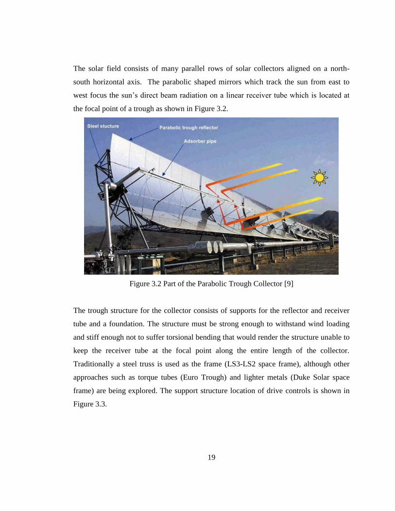
The solar field consists of many parallel rows of solar collectors aligned on a north-

south horizontal axis. The parabolic shaped mirrors which track the sun from east to

west focus the sun’s direct beam radiation on a linear receiver tube which is located at

the focal point of a trough as shown in Figure 3.2.

Figure 3.2 Part of the Parabolic Trough Collector [9]

The trough structure for the collector consists of supports for the reflector and receiver

tube and a foundation. The structure must be strong enough to withstand wind loading

and stiff enough not to suffer torsional bending that would render the structure unable to

keep the receiver tube at the focal point along the entire length of the collector.

Traditionally a steel truss is used as the frame (LS3-LS2 space frame), although other

approaches such as torque tubes (Euro Trough) and lighter metals (Duke Solar space

frame) are being explored. The support structure location of drive controls is shown in

Figure 3.3.

20

Figure 3.3 Schematic of a Solar Collector Assembly [22]

Luz is the company which constructed the SEGS plant in California and developed a

new trough structure design. LS-1 trough structure design is used in SEGS I-II and LS-3

is used in SEGS II-VII. The final through structure design is the Luz LS-3 and is used in

the newest SEGS plants [28].

A consortium of European companies and research laboratories known as EuroTrough

have developed next-generation trough concentrator. Based on these studies a torque

box concentrator concept has been selected. It eliminates many of the problems

associated with the LS-2 and LS-3 collectors. EuroTrough has weighs less and suffers

less deformations of the collector structure due to dead weight and wind loading than the

reference designs [28,29].

Duke Solar, North Carolina, developed an aluminium space frame that resulted in an

advanced-generation trough concentrator design. Weight, manufacturing simplicity,

21

corrosion resistance, manufactured cost, and installation ease are unique features of this

design [28]. All three models are shown in Figure 3.4.

Figure 3.4 LS-3 space frame, EuroTrough torque-box, and Duke Solar Space Frame

concentrator designs [28]

A heat transfer fluid (HTF) is circulated through the collector field during the day. It is

heated as it circulates through the receiver tubes and returns to heat exchangers in the

power block. In the power block the hot HTF is used to generate superheated steam. The

superheated steam is then forwarded to steam turbines that drive electricity generators

[11].

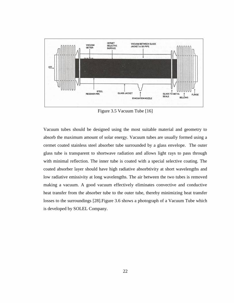
The HTF circulates in a receiver tube and absorbs concentrated solar radiation. This

receiver tube is a vacuum tube designed specifically to maximize the amount of thermal

energy adsorbed based on cost constraints. Figure 3.5 shows a diagram of a typical

vacuum tube.

22

Figure 3.5 Vacuum Tube [16]

Vacuum tubes should be designed using the most suitable material and geometry to

absorb the maximum amount of solar energy. Vacuum tubes are usually formed using a

cermet coated stainless steel absorber tube surrounded by a glass envelope. The outer

glass tube is transparent to shortwave radiation and allows light rays to pass through

with minimal reflection. The inner tube is coated with a special selective coating. The

coated absorber layer should have high radiative absorbtivity at short wavelengths and

low radiative emissivity at long wavelengths. The air between the two tubes is removed

making a vacuum. A good vacuum effectively eliminates convective and conductive

heat transfer from the absorber tube to the outer tube, thereby minimizing heat transfer

losses to the surroundings [28].Figure 3.6 shows a photograph of a Vacuum Tube which

is developed by SOLEL Company.

23

Figure 3.6 A photo of Vacuum Tube Connection [30]

The selection of the type of HTF is also important. Biphenyl-diphenyl-oxide, known by

the trade name TherminolVP-1, is used in the latest SEGS plants. It has excellent

stability, safety and environmental protection. TherminolVP-1 also has some limitations

which are the temperature range, cost, the need for heat exchange equipment to transfer

thermal energy to the power cycle and the oil has a high vapour pressure, so it is difficult

to store thermal energy [28,31].

Thermal losses, tracking precision, surface properties cleanliness of reflectors, incident

solar radiation, HTF flow rate and solar field inlet temperature affect the solar field

outlet temperature.

24

3.2. Power Cycle Model

The objective of the parabolic trough plant is to generate electricity. The larger system

consists of a solar collector field linked to a Rankine cycle via a series of heat

exchangers. Figure 3.7 shows the flow diagram of the SEGS VI plant. A traditional

Rankine cycle is used as the power cycle in these solar electric generating systems. The

power cycle is driven by heat transfer from the heat transfer fluid (HTF). The HTF is

heated as it circulates through the receiver and returns to the power cycle by an

expansion vessel. The average temperature and the total volume of the HTF change

significantly throughout the day. The expansion vessel accommodates these effects. The

HTF is pumped from the expansion vessel and delivered to two heat exchanger systems.

One of the heat exchanger systems consists of a superheater, steam generator and

preheater and the other heat exchanger system is the reheater.

Figure 3.7 Flow Diagram of the SEGSVI Plant [21]

25

These heat exchanger systems are counterflow with the HTF and water in the Rankine

cycle flowing in opposite directions. The HTF enters the superheater at a high

temperature before passing to the boiler in which the water in the Rankine cycle changes

phases from liquid to steam. The last step for the HTF is to pass through the preheater

where it heats the liquid water (termed feedwater) entering the heat exchanger system.

The cooled HTF that leaves this heat exchanger system is then recirculated through the

solar field. The superheated steam leaving this heat exchanger system is then fed to the

high pressure turbine to produce electricity. Both high and low pressure turbines are

used with reheat occurring between these turbines stages. The high pressure turbine has

two and the low pressure turbine has five steam extractions that flow to the feedwater

heaters. This extracted steam is used to heat the feedwater before it enters the pre-heater

described above to increase the efficiency of the Rankine cycle. The remaining steam

leaving the low pressure turbine is condensed in a standard condenser. Before returning

to the preheater to complete the cycle, the liquid feedwater leaving the condenser passes

through three low pressure feedwater heaters, a deaerator and two high pressure

feedwater heaters.

3.3. Flow and Temperature – Entropy Diagrams

Kearney analyzed a plant with 35 MW gross power and 100% solar operation [16].

Figure 3.8 shows the flow diagram of the power-cycle. A temperature-entropy diagram

of the cycle with all corresponding intermediate state points is shown in Figure 3.9.

26

Figure 3.8 Flow Diagram for Power Cycle -state points labeled.

27

Figure 3.9 Temperature- Entropy Diagram of Power Cycle at Reference State (35

MW,100% solar )[16]

State (9) must be incorrect, as moving from state (8) to state (9) through expansion in a

an adiabatic turbine would violate the second law. An isentropic efficiency is assumed

0.88 in the turbine section from (8) – (9). In the present work at state (9) the entropy and

enthalpy are recalculated, assuming the pressures provided are correct [16].

3.4. TRNSYS and STEC Library

TRNSYS is software which is developed primarily at The University of Wisconsin and

is a complete and extensible simulation environment for the transient simulation of

systems. Models of individual components can be created and these individual models

are called Types. These models of individual components are then connected within

TRNSYS and simulations for the larger system run. Each Type of component is

described by a mathematical model in the TRNSYS simulation engine [32].

28

STEC (Solar Thermal Electric Components) is a TRNSYS library. It is developed by

DLR (German Aerospace Centre) and Sandia National Laboratory and consists of

models suitable for Rankine and Brayton cycles, concentrating solar thermal systems

(central receiver, heliostat field, and parabolic trough models), and storage [33].The

software and documentation for TRNSYS [32] and STEC [33] contain numerous

examples and tutorials for how to develop energy models of simple energy systems, and

interested readers are referred to these software and documentation for introductory

information on how to use TRNSYS and STEC.

In this work a model of a solar thermal electric generating system using parabolic trough

collector was created using components from the STEC library. Detailed information

about these components is given below. A schematic of the model as shown in the

TRNSYS simulation studio is shown in Figure 3.10. Both the high pressure (HP) and

low pressure (LP) turbines are modeled using several components which are grouped

into a single turbine macro. In Figure 3.10, the HP and LP turbine macros are shown as a

single icon to aid in understanding the larger system. In Figure 3.10, material and

information flows are indicated by connections between two components.

Figure 3.10 The SEGS VI TRNSYS Model

29

It is important to properly specify the required variables for each component while

creating a simulation studio. The user right clicks on the component icon to change the

parameters, inputs, derivatives and view the outputs. The parameters, inputs, outputs,

and derivatives are all available in separate windows, with the output window being just

for informational purposes. A screen shot of the parameter window with tabs for the

Input, Output, and Derivative windows is shown in Figure 3.11.

.

Figure 3.11 Parameters Window

An important step in simulating the operation of a component is specifying the values of

transient variables through a link to another component. A link is used between two

components so that information flow can occur. To specify the details of the link

between two components, the user should use the graphical user interface (GUI) opened

by double-clicking on the link. To specify the connection between two components, the

user connects the outputs of the first component (left-side) to the required inputs of the

second component (right-side). Additionally, users can only connect variables of the

30

same dimension, i.e. 'heat' to 'heat' [32]. Any input that is left unconnected is assumed to

be constant at its initial value for all time [32]. Figure 3.12 shows how a sample

connection is created.

Figure 3.12 Sample Connection Window Showing Connection Between Weather Data

(outputs, left column) and Parabolic Trough Collector (inputs, right column)

31

The same connection information in Figure 3.12 is also presented in Table 3.1.

According to table and figure, one can easily see that all connected variables have the

same dimension. For conciseness and clarity, all other connections in this TRNSYS

model will be communicated through tables such as Table 3.1.

Table 3.1 Description of Connections

Type 109-TMY 2 Trough

Solar azimuth angle Sun azimuth

Solar zenith angle Sun zenith

Beam radiation on tilted surface DNI –Direct Normal Irradiance

Wind velocity Wind speed

Ambient temperature Ambient temperature

3.5. Superheater

The superheater used in this system is a tube and shell heat exchanger. The effectiveness

of the superheater is related to its thermal performance. The heat exchanger

effectiveness () is defined as the actual heat transfer realized between streams ( ) over

the maximum heat transfer possible for the given streams ( max) [16]. Figure 3.11

shows the flow diagram for the superheater.

(3.1)

32

Figure 3.13 Flow diagram of superheater

STEC built-in component Type 315 is used to model the superheater. Values for

constant parameters and initial conditions used are given in Table 3.2. For this study the

necessary properties are taken from a technical description [23].

Table 3.2 Constant Parameters and Initial Conditions for Superheater

Parameter Input Unit

Overall heat transfer coefficient 1015.97 kJ/hr.K

Hot side inlet temperature 390.56 °C

Hot side flow rate 396.4 kg/s

Cold side inlet temperature 313.89 °C

Cold side flow rate 38.969 kg/s

Cold side quality 1 -

Cold side outlet pressure 100 bar

Hot side specific heat 2.59 kJ/kg.K

For all heat exchangers the hot side is the HTF flowing from the collector while the cold

side is the water in the Rankine cycle. The transient values for inputs for the superheater

33

are defined by the input connections given in Table 3.3, while the outputs that define

transient inputs for other components are given in Table 3.4.

Table 3.3 Input Links for the Superheater

Input Output

Superheater Splitter

Hot side flow rate Outlet flow rate2

Superheater Boiler

Cold side inlet temperature Cold side outlet temperature

Cold side flowrate Cold side outlet flowrate

Cold side quality Cold side quality

Superheater X2H

Cold side outlet pressure Steam pressure

Table 3.4 Output Links for the Superheater

Input Output

Boiler Superheater

Hot side inlet temperature Hot side outlet temperature

Hot side flowrate Hot side flowrate

Cold side outlet pressure Cold side inlet pressure

X2H Superheater

Steam temperature Cold side outlet temperature

Steam quality Cold side outlet quality

Steam flow rate Cold side flow rate

34

3.6. Boiler (Steam Generator)

The feedwater enters the shell side of the boiler and exits as a saturated vapor. The boiler

effectiveness is related to the number of transfer units (NTU). Figure 3.14 shows the

flow diagram for the boiler. When the saturated liquid changes phase from saturated

liquid feedwater to steam its capacitance infinite [16,34]. The minimum capacitance of

the fluid is

(3.2)

Figure 3.14 Flow diagram of boiler (steam generator)

STEC built-in component Type 316 is used to model a boiler. The parameters that are

used to model the boiler STEC Type316 are given in Table 3.5.

35

Table 3.5 Constant Parameters and Initial Conditions for Boiler



Hot side inlet temperature 377.22 °C


Cold side inlet temperature 313.89 °C


Cold side inlet quality 0 -

Cold side outlet pressure 103.42 bar


The transient values for inputs for the boiler are defined by the input connections given

in Table 3.6, while the outputs that define transient inputs for other components are

given in Table 3.7.

Table3. 6 Input Links for the Boiler

Input Output

Boiler Preheater


Cold side inlet quality Cold side outlet quality

Boiler Superheater




36

Table 3.7 Output Links for the Boiler

Input Output

Preheater Boiler




Superheater Boiler


Cold side flowrate Cold side outlet flowrate

Cold side quality Cold side outlet quality

Feedwater pump Boiler

Desired mass flow rate Cold side flow rate demand

3.7.Preheater

The preheater is also a type of heat exchanger and is used to raise the temperature of the

feed water leaving the system of feed water heaters. While modeling the preheater, it is

assumed that the feedwater outlet state will be a saturated liquid at the outlet pressure of

the preheater [16]. The heat transfer to the feedwater is calculated as

) (3.3)

Figure 3.15 shows the flow diagram for the preheater.

37

Figure 3.15 Flow diagram of Preheater

STEC built-in component Type 315 is used to model a preheater. The parameters that

are used to model the preheater STEC Type315 are given in Table 3.8

Table 3.8 Constant Parameters and Initial Conditions for Preheater

The transient values for inputs for the preheater are defined by the input connections

given in Table 3.9. while The outputs that define transient inputs for other components

are given in Table 3.10.


Overall heat transfer coefficient

175710.2297 kJ/hr.K

Hot side inlet temperature 317.78 ˚C


Cold side inlet temperature 234.83 ˚C





38

Table 3.9 Input Links for the Preheater

Input Output

Preheater Boiler


Hot side flowrate Hot side outlet flowrate


Preheater Feedwaterheater


Cold side inlet flowrate Cold side outlet flowrate

Table 3.10 Output Links for the Preheater

Input Output

Boiler Preheater


Cold side inlet quality Cold side outlet quality

Mixer Prehater

Inlet flowrate 2 Hot side flowrate

3.8. High Pressure and Low Pressure Turbine

Both high and low pressure turbines are used. Superheated steam leaving the superheater

at a high temperature and high pressure enters the high pressure turbine. The expansion

of the steam as it moves from a high pressure to a lower pressure converts the steam’s

enthalpy to shaft work. The shaft work created by the rotating shaft is converted to

electrical energy through a generator. Steam is extracted at intermediate points during

the expansion process and fed to the feed water heaters. The turbines are modeled as a

series of turbine stages connected in series. Each stage consists of a turbine and a

splitter. One outlet of the splitter is connected to the next turbine stage (or is the outlet of

the larger turbine if the last turbine stage) while the splitter’s other outlet is connected to

a feedwater heater. Figure 3.16 shows a flow diagram for a turbine stage.

39

Figure 3.16 Flow diagram of Turbine Stage Consisting of a Turbine and a Splitter.

The high pressure (HP) turbine consists of two stages and the low pressure (LP) turbine

consists of five stages. Between the HP and LP turbines steam passes through the

reheater to increase the cycle efficiency. The thermodynamic performance of each

turbine stage is described by its isentropic efficiency [16,22,34]. The isentropic

efficiency of a turbine stage is equal to the change in enthalpy of the fluid to the change

in enthalpy of an isentropic (adiabatic and reversible) turbine:

(3.4)

where hsteam,out,S is the enthalpy that would have occurred at the outlet of the isentropic

turbine. The total power of the turbine is equal to the mass flow rate through each

turbine stage multiplied by the mass specific work of that stage. The steam mass flow

rate through each stage is equal to turbine inlet mass flow rate minus the total mass flow

rates of the steam extracted to flow to the feedwater heaters in the previous stages. The

power for each turbine stage is as follows:

40

(3.5)

(3.6)

(3.7)

(3.8)

(3.9)

(3.10)

(3.11)

The total output equals the sum of the output from each turbine section.

(3.12)

For the HP and LP turbines, STEC components Type 318 (turbine) and Type 389

(splitter) are used to model a single turbine stage. The TRNSYS model of the high

pressure turbine with two extracts is shown in Figure 3.17

Figure 3.17 STEC Components Turbine and Splitters

41

The parameters that are used to model the HP turbine’s 1st stage are given in Table 3.11

and Table 3.12.

Table 3.11 Constant Parameters and Initial Conditions for HP turbine 1st stage


Design inlet pressure 100 bar

Design outlet pressure 33.61 bar

Design flow rate 38.6415 kg/s

Design inner efficiency 0.8376 -

Turbine outlet pressure 33.61 bar

Turbine inlet flowrate 38.6415 kg/s

Turbine inlet enthalpy 3005 kJ/kg

The controlled splitter has one inlet and two outlets. The mass flow rate for outlet one

goes to a feedwater heater, and the remaining flow leaves from outlet two and goes to

the next turbine stage. The enthalpies for the splitter’s outlets one and two are equal to

its inlet enthalpy. In this model the pressure information is transported in a direction

opposite to the mass flow, such that the turbine stage’s inlet pressure is fixed by the

turbine stage’s outlet pressure, and the turbine stage’s outlet pressure is fixed by the inlet

pressure of the next turbine stage.

42

Table 3.12 Initial Parameters for the HP Turbine 1st stage splitter


Demanded flow out 1 2.9311 kg/s

Inlet flow rate 38.6414 kg/s

Outlet pressure 2 33.61 bar

Inlet enthalpy 3005 kJ/kg

The parameters that are used to model the HP turbine 2nd stage are given in Table 3.13

Table 3.13 Constant Parameters and Initial Conditions for HP Turbine 2nd Stage


Design inlet pressure 33.61 bar







The link between the HP turbine stage 1 and splitter is shown Table 3.14. A parallel set

of links are used for the HP turbine’s second stage and all LP turbine stages.

43

Table 3. 14 Input and Output Links for the Turbine Stage

Input Output

HP Turbine Stage 1 Splitter

Turbine outlet flowrate Inlet flowrate

Turbine outlet enthalpy Inlet enthalpy

Splitter HP Turbine Stage 1

Inlet Pressure Turbine outlet pressure

The parameters that are used to model the HP turbine 2nd stage are given in Table 3.15

Table 3.15 Initial Parameters for the HP Turbine 2nd Stage Splitter

Demanded flow out 2.8009 kg/s

inlet flowrate 35.7326 kg/s

Outlet pressure2 18.58 bar


3.9. Reheater

The reheater is also a shell and tube heat exchanger. In this cycle after leaving the HP

turbine the steam goes to the reheater and the temperature increases so that the system

efficiency increases. The reheater model is the same as the superheater model and same

equations are used. STEC built-in component Type 315 is used to model the reheater.

Values for constant parameters and initial conditions used are given in Table 3.16.

44

Table 3.16 Constant Parameters and Initial Conditions for the Reheater



Hot side inlet temperature 390.56 ˚C







The transient values for inputs for the reheater are defined by the input connections

given in Table 3.17 while the outputs that define transient inputs for other components


Table 3.17 Input Links for the Reheater

Input Output

Reheater HP Turbine

Cold side flowrate Splitter2 outlet flowrate

Reheater HTF Splitter

Hot side flowrate Outler flowrate1

Reheater X2H2

Cold side outlet Pressure Steam pressure

45

Table 3.18 Output Links for the Reheater

Input Output

HP Turbine Reheater

Splitter outlet pressure 2 Cold side inlet pressure

Mixer Reheater

Inlet flowrate 1 Hot side flowrate

X2H2 Reheater

Steam temperature Cold side outlet temperature

Steam quality Cold side outlet quality

Steam flowrate Cold side flowrate

X2H2 is a STEC component which converts steam properties given by T, p, and x used

in the superheater and reheater components to h and p used in the turbine stage

components [33].

3.10. Low Pressure (LP) Turbine

The LP turbine stages are modeled in a manner parallel to the HP turbine stages. The

details on the input and output links and the initial conditions and constants are given in

Tables 3.19-3.27 for each LP turbine stage.

For each LP turbine stage, STEC components Type 318 (turbine) and Type 389 (splitter)

are used as shown in Figure 3.18.

Figure 3.18 STEC Components Turbine and Splitter

46

Table 3.19 Initial Conditions and Constants for LP turbine 1st stage









By pass indicator 1 -

Table 3.20 Initial parameters for LP turbine 1st stage splitter





Table 3.21 Initial Conditions and Constants for LP turbine 2nd stage










47

Table 3.22 Initial Parameters for LP Turbine 2nd Stage Splitter





Table 3.23 Initial Conditions and Constants for LP Turbine 3rd Stage










Table 3.24 Initial Parameters for LP Turbine 3rd Stage Splitter





48

Table 3.25 Initial Conditions and Constants for LP Turbine 4th Stage










Table 3.26 Initial Parameters for LP Turbine 4th Stage Splitter


Inlet flowrate 27.4158 kg/s



49

Table 3.27 Initial Conditions and Constants for LP Turbine 5th Stage










3.11. Condenser

The condenser is a shell and tube heat exchanger. On the tube side cooling water is

flowing and on the shell side the steam from the LP turbine is condensing. The

condenser condenses the steam from the LP turbine (steam inlet) to a liquid so that the

fluid can be easily pumped back to the boiler (condensed feed water, outlet). Figure 3.19

shows the flow diagram for the condenser.

50

Figure 3. 19 Flow Diagram of Condenser

(3.13)

The condenser effectiveness is the ratio of the heat transfer between cooling water and

condensing steam to the maximum heat transfer between these streams [16].

(3.14)

(3.15)

The condenser is modeled using STEC component Type 383. The parameters that are

used to model the condenser STEC Type383 are given in Table 3.28

51

Table 3.28 Initial Conditions and Constants for the Condenser


Cooling water inlet temperature 25.5 ˚C

Steam enthalpy inlet 2348.1 kJ/kg

Steam mass flow rate 26.4820 kg/s

Condensate inlet flow rate 4.4871 kg/s

Condensate inlet temperature 52.889 ˚C

Condensate inlet Quality 0 -

The transient values for inputs for the condenser are defined by the input connections



Table 3.29 Input Links for the Condenser

Input Output

Condenser LP Turbine

Steam enthalpy inlet Stage 5 Turbine outlet enthalpy

Steam mass flowrate Stage 5 Turbine outlet flowrate

Condenser Feed water heater

Condensate inlet flowrate Hot side outlet flowrate

Condensate inlet quality Hot side outlet quality

52

Table 3.30 Output Links for the Condenser

Input Output

Condensate pump Condenser

Inlet fluid temperature Condensing temperature

Inlet mass flowrate Condensate flowrate

LP Turbine Condenser

Turbine outlet pressure Condensing pressure

3.12. Pump

In this solar electric generating system there are three pumping processes. The pumps

increase the pressure of the feed water and heat transfer fluid. One pump is a condensate

pump and is located at the condenser outlet. The second is a feed pump and is located at

the deaerator outlet. The last one is a heat transfer fluid pump and is located before the

collector field. Figure 3.20 shows the flow diagram for the pump. The STEC component

Type 300 is used to model a pump. Pump performance is characterized by its isentropic

efficiency [16,34].The isentropic efficiency of the pump is:

(3.16)

where hfeedwater,out,S is the enthalpy that would have occurred were the pumping process

isentropic. The work performed by the pump per unit mass is the change

(3.17)

The parameters that are used to model the condensate pump, feed water pump, and heat

transfer fluid pump are given in Table 3.31-Table 3.36.

53

Figure 3.20 Flow Diagram of a Pump

Table 3.31 Initial Conditions and Constants for the Condensate Pump


Inlet fluid temperature 41.439 ˚C

Inlet mass flow rate 30.969 kg/s

Desired mass flow rate 30.969 kg/s

Maximum flow rate 30.969 kg/s

Fluid specific heat 4.19 kJ/kg.K

Maximum power 190000 W

Table 3.32 Input and Output Links for the Condensate Pump

Input Output

Pump Condenser

Inlet fluid temperature Condensing temperature

Inlet mass flowrate Condensate flowrate

Feed water heater1 Pump

Cold side fluid temperature Outlet fluid temperature

Condensate inlet flowrate Outlet flowrate

54

Table 3.33 Initial Conditions and Constants for the Feed Pump







Maximum power 8.8 x 105

W

Table 3.34 Output and Input Links for Feedwater Pump

Input Output

Pump Condenser

Inlet fluid temperature Feed water outlet temperature

Inlet mass flow rate Feed water outlet flow rate

Pump Boiler

Desired mass flow rate demand Cold side flow rate demand

Feed water heater1 Pump

Cold side fluid temperature Outlet fluid temperature

Condensate inlet flow rate Outlet flow rate

55

Table 3.35 Initial Conditions and Constants for the HTF Pump







Maximum power 1.6 x 107

W

Table 3.36 Output and Input Links for HTF Pump

Input Output

Pump Mixer

Inlet mass flow rate Outlet flowrate 1

Trough Pump

Inlet temperature solar field Outlet fluid temperature

3.13.Deaerator

The deaerator preheats the feed water for the steam generator. Steam extracted from the

1st stage of the LP turbine is directly mixed with feed water. At the outlet of the

deaerator there is a feed pump which increases the fluid pressure to boiling pressure. The

deaerator is a mixing device with three inlets and single outlet stream [16]. Figure 3.21

shows the flow diagram for the deaerator. The three inlets are the drain water from the

high pressure feedwater heaters, the extracted steam from the first stage of the low

pressure turbine, and the feedwater from the low pressure feed water heaters. The total

mass flow rate is the sum of the three inlet.

(3.18)

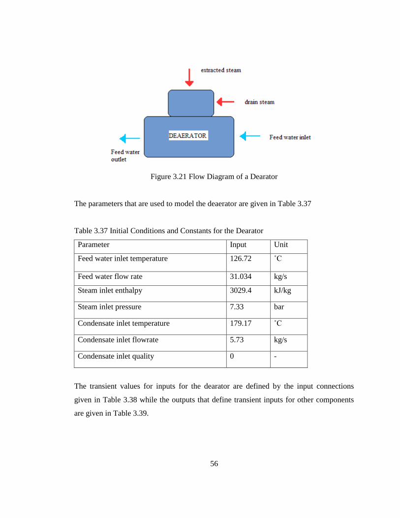
56

Figure 3.21 Flow Diagram of a Dearator

The parameters that are used to model the deaerator are given in Table 3.37

Table 3.37 Initial Conditions and Constants for the Dearator


Feed water inlet temperature 126.72 ˚C

Feed water flow rate 31.034 kg/s

Steam inlet enthalpy 3029.4 kJ/kg

Steam inlet pressure 7.33 bar


Condensate inlet flowrate 5.73 kg/s

Condensate inlet quality 0 -

The transient values for inputs for the dearator are defined by the input connections



57

Table 3. 38 Input Links for Dearator

Input Output

Dearator Feed water heater 3

Feedwater inlet temperature Cold side outlet temperature

Feed water flowrate Cold side outlet flowrate

Dearotor LP Turbine Splitter1

Steam inlet enthalpy Outlet enthalpy

Steam inlet pressure Outlet pressure

Table 3. 39 Output links for the Dearator

Input Output

Feed water pump Dearator

Inlet fluid temperature Feed water outlet temperature

Inlet mass flowrate Feed water outlet flowrate

LP Turbine Splitter1 Dearator

Demanded Flow out 1 Required steam flowrate

3.14. Feedwater heaters

A feedwater heater increases the steam temperature and thereby reduces the heat

addition from the collector loop and increases the system efficiency.

There are three zones in which the heat transfer occurs in a closed feedwater heater.

These zones are the desuperheating zone, condensing zone, subcooling zone. The steam

is reduced to a saturated vapor in the desuperheating zone and in the condensing zone

steam condenses from a saturated vapor to a saturated liquid. In the subcooling or drain

cooling zone the condensed steam is cooled to a temperature below its saturation

temperature. The size and conductance determine the feedwater heater’s overall heat

transfer factor (UA). It is assumed here that the condensing zone of each feedwater

58

heater is sufficiently large in comparison to the desuperheating and subcooling zones

that the desuperheating and subcooling zones can be neglected in the model. An overall

UA for each feedwater heater is defined assuming steam is condensing throughout the

length of the feedwater heater [16].

The preheater model calculates the required steam mass flowrate that keep the water

level in this heat exchanger constant. Effective heat transfer factor is described the heat

transfer characteristic [29].UA is evaluated as a function of the cold side flow rate by

(3.19)

Figure 3.22 and Figure 3.23 shows the flow diagram for the feed water heater. For feed

water heater STEC component Type 317 is used to model a feed water heater. The

parameters that are used to model the feed water heater STEC Type317 are given in

Table 3.40.

Figure 3.22 Flow Diagram of a Feedwater Heater

59

Figure 3.23 STEC Component Feedwater Heater

Table 3.40 Initial Conditions and Constants for the 1st Feedwater Heater (FWH1)


Cold fluid specific heat capacity 4.18 kJ/kg.K

Overall heat transfer factor 456.79 kW/K

Cold side ref flow rate 31.03 kg/s

Power law exp 0.8 -

Hot side inlet enthalpy 2528.1 kJ/kg

Hot side inlet pressure 0.2797 bar


Cold side inlet flowrate 31.03 kg/s




The transient values for inputs for the FWH1 are defined by the input connections given

in Table 3.41 while the outputs that define transient inputs for other components are

given in Table 3.42

60

Table 3.41Input Links for Feedwater Heater1

Input Output

Feed water heater1 Condensate pump

Cold side inlet temperature Outlet fluid temperature

Cold side inlet flowrate Outlet flowrate

Feed water heater 1 LP Turbine splitter4

Hot side inlet enthalpy Outlet enthalpy 1

Hot side inlet pressure Outlet pressure 1

Feed water heater 1 Feed water heater 2



Table 3. 42 Output Links for Feedwater Heater1

Input Output

Condenser Feed water heater 1



LP Turbine splitter4 Feed water heater 1

Demanded flow out 1 Demanded hot inlet flowrate

Hot side inlet pressure Outlet pressure 1

Feed water heater 2 Feed water heater 1


Cold side inlet flowrate Cold side outlet flowrate

A parallel system of connections exists for all other closed feed water heater. Details of

these links are not presented herein for brevity.

61

Table 3.43 Initial Conditions and Constants for the 2nd Feedwater Heater (FWH2)





Power law exp 0.8 -








62

Table 3.44 Initial Conditions and Constants for 3rd Feedwater Heater (FWH3)





Power law exp 0.8 -





Condensate inlet temperature - ˚C

Condensate inlet flowrate - kg/s


Table 3.45 Initial Conditions and Constants for 5th Feedwater Heater (FWH5)





Power law exp 0.8 -








63

Table 3. 46 Initial Conditions and Constants for the 6th Feedwater Heater (FWH6)





Power law exp 0.8 -

Hot side inlet enthalpy 2807 kJ/kg




Condensate inlet temperature - ˚C

Condensate inlet flowrate - kg/s


3.15. Weather data

This component reads weather data at regular time intervals from a data file. It can

easily convert the data to the desired units and make it available to other TRNSYS

components. Type 109-TMY2 reads a weather data file in the standard Typical

Meteorological Year (TMY2) format. The TMY2 format is used by the National Solar

Radiation Data Base (USA) [35].

A TMY is a data file which provides a standard for hourly values of solar radiation and

meteorological elements for a 1 year period. The TMY data set is constructed by

analyzing a multi-year set of data using statistical methods, and then for each month the

year with the “most typical” weather data is selected. Thus a TMY data set may use data

from 1982 for January, 1995 for February, 1991 for March, etc. By using actual rather

than average weather data for each month, fluctuations between cloudy and sunny days

is captured better and these data sets are preferred for simulating the performance of

64

solar energy conversion systems [36]. The initial parameters that are used to model the

weather data file Type 109 are given in Table 3.47.

Table 3.47 Initial parameters for weather data file


Ground reflectance 0.2 -

Slope of surface 0 degrees

Azimuth of surface 0 degrees

The transient values for inputs for the weather data are defined by the input connections

given in Table 3.48

Table 3.48Input Links for Weather Data File

Input Output

Weather data Trough-2

Solar azimuth angle Sun Azimuth

Solar zenith angle Sun Zenith

Beam radiation on tilted surfaces DNI-Direct Normal Irradiance

Wind Velocity Wind Speed


In Appendix B detailed information on the TMY2 data and format is presented.

3.16. Expansion vessel

The average temperature of the HTF changes during the day which causes the HTF to

undergo significant changes in volume. The expansion vessel accommodates the

expansion and contraction of the HTF. The expansion vessel is taken from the TRNSYS

library. Figure 3.24 shows the flow diagram for the expansion vessel. The parameters

that are used to model the expansion vessel Type 4-a are given in Table 3.49

65

Figure 3.24 Flow diagram of expansion vessel

Table 3.49 Initial parameters for expansion vessel


Tank volume 287 m3


Fluid density 704 kg/m3

Tank loss coefficient 0 kJ/hr.m2.K

Boiling point 257 ˚C

Hot side temperature 390.56 ˚C

Hot side flowrate 396.4 kg/s

Cold side temperature 297 ˚C

Cold side flowrate 0 kg/s

Environment temperature 30 ˚C

The transient values for inputs for the expansion vessel are defined by the input

connections given in Table 3.50 while the outputs that define transient inputs for other

components are given in Table 3.51

66

Table 3.50 Input Links for the Expansion Vessel

Input Output

Expansion vessel Trough-2

Hot side Temperature Outlet Temperature Solar Field

Hot side Flowrate Flow rate Solar Field

Table 3. 51 Output Links for the Expansion Vessel

Input Output

Splitter Expansion Vessel

Inlet Flowrate Flow rate to heat source

3.17. Parabolic Trough Field

The parabolic trough collector component is developed using Lippke’s model [23].

To account for changing fluid temperature, an integrated efficiency equation is used

which calculates the demanded mass flow rate of the heat transfer fluid to achieve a

user-defined outlet temperature Tout [26].

Using

Qnet = Qabs – Qpipe

Qnet : net power

Qabs : ratio of absorbed power (%) (3.20)

Qpipe : accounts for losses in the piping.

The thermal efficiency is

= +D (3.21)

In this equation,

A : optical efficiency of the trough and the absorptivity of the selective coating without

considering the losses at the end of a collector row.

67

B, C and D : Describe the heat losses of the heat collecting element (HCE) as a function

of operating conditions.

ΔT : Temperature difference between the HTF and the ambient (K).

K:incident angle modifier

I: Direct Normal Insolation (W/m2)

Qabs : ratio of absorbed power (%)

The model considers electrical parasitic losses during startup, shutdown, pumping and

tracking. At high wind speeds the system automatically shutdown [33].

Table 3.52 shows the thermal performance coefficient. Parabolic trough collector model

use the third line data which is black chrome and vacuum.

Table 3.52 Thermal performance coefficients [23].

vwind : Wind velocity

STEC component Type 396 is used to model parabolic trough collector model. The

parameters that are used to model the parabolic trough collector STEC Type 396 are

given in Table 3.53

A B C D

Cermet, vacuum 73.3 -0.007276 -0.496 -0.0691

Cermet, air 73.4 -0.004683 -14.40 -0.0637

Cermet, bare 74.7 -0.042-0.00927 x vwind/K 0.00 -0.000731xI

Black

Chrome,vacuum

73.6 -0.004206 7.44 -0.0958

Black Chrome, air 73.8 -0.006460 -12.16 -0.0641

68

Table3.53 Initial Conditions and Constants for the Parabolic Trough Collector


A loss coeff. 73.6 -

B loss coeff. -0.0042 -

C loss coeff. 7.40 -

Cw loss coeff. 0 -

D loss coeff. -0.096 -

Clean reflectivity 0.94 -

Length of SCA(Solar Collector Area) 47 m

Aperture With of SCA(Solar Collector Area) 5 m

Focal length of SCA(Solar Collector Area) 5 m

Row Spacing 15 m

Total field Area 182000 m2

Pump Max. Power 1600 kW

Pump Max Flowrate 396.4 kg/s

Demanded Outlet Temperature 390.56 ˚C

Inlet Temperature Solar Field 297.78 ˚C

Cleanliness Solar Field 0.95 -

Specific Heat HTF 2.59 kJ/kg.K

Ambient temperature 30 ˚C

Wind speed Limit for tracking 5 m/s

The transient values for inputs for the Trough are defined by the input connections given

in Table 3.54 while the outputs that define transient inputs for other components are

given in Table 3.55.

69

Table 3. 54 Input Links for the Trough

Input Output

Trough-2 Weather data

Sun Azimuth Solar azimuth angle

Sun Zenith Solar zenith angle

DNI-Direct Normal radiation Beam radiation on tilted surfaces

Wind Speed Wind Velocity


Trough-2 HTF Pump

Inlet Temperature Solar Field Outlet Fluid Temperature

Table 3.55 Output Links for the Trough

Input Output

Expansion vessel Trough-2

Hot side Temperature Outlet Temperature Solar Field

Hot side Flowrate Flow rate Solar Field

3.18. Model Capabilities and Limitations

The solar field model is computationally efficient. More complex and transient

thermodynamics models can be implemented. The solar thermal power community

prefers this software because of the availability of the TRNSYS source code [32].

Users easily choose a time period and analyze one or more locations performance and

get a Microsoft Excel output. Using the software’s online plotter the results can be

drawn. The model of the system consists of 34 components and requires a fairly large

amount of data. Each component’s data may have to be changed if the system is

70

redesigned. In this work the approximate time to run one annual simulation takes 4-5

seconds.

Before running a simulation, TRNSYS converts the model of the energy system

developed using the graphical user interface into called a “Deck” file. The Deck file for

the present system is presented in Appendix C. This Deck file contains a complete

description of the system modeled in TRNSYS.

71

CHAPTER 4

RESULTS

4.1 Model Validation

The aim of this study is to create a model that correctly predicts SEGS VI plant behavior

and apply the same model to Turkey. In order to validate the model its results are

compared with measured plant data which is taken from the Kearney et al. technical

description and the TRNSYS model predictions [23]. The study by Kearney et al. shows

how their model’s predictions compare to real operating data for a sunny summer and a

cloudy winter day. Figure 4.1 shows the insolation, temperature and wind speed

measured during a clear sunny day on July 18, 1991 in California, Daggett.

Figure 4.1 Weather Conditions July 18, 1991[26]

72

Figure 4.2 Weather Conditions July 18, 1991 TRNSYS results

Figure 4.2 shows results from the TRNSYS modeled developed herein for the same

location and data. Comparison of TRNSYS results with predictions reported in the

literature shows that the DNI, wind and ambient temperature results are generally close

to each other. Atmospheric conditions and large air mass changes throughout the day

affect the collector location, orientation and tracking capability. The insolation results

from Figures 4.1 and 4.2 are presented in Figure 4.3 and it is easily seen that the DNI

results predicted by the current model and that reported in the literature are close to each

other.

73

Figure 4.3 Comparison of TRNSYS Results and Real data plant DNI July 18, 1991

Figure 4.4 shows measured and predicted gross power output results on July 18,1991 as

reported in [26] and in Figure 4.5 the predictions from the current model are presented.

As seen in Figure 4.6 in which the present TRNSYS simulation results are compared to

that presented in the literature, the sunny day power predictions match well in the

morning, but have error in the afternoon when the ambient temperature is higher.

However, within the context of the present study these errors are considered to be

acceptable.

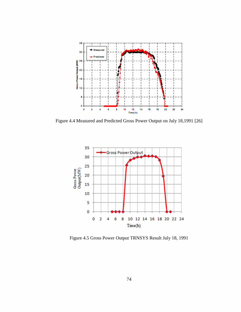
74

Figure 4.4 Measured and Predicted Gross Power Output on July 18,1991 [26]

Figure 4.5 Gross Power Output TRNSYS Result July 18, 1991

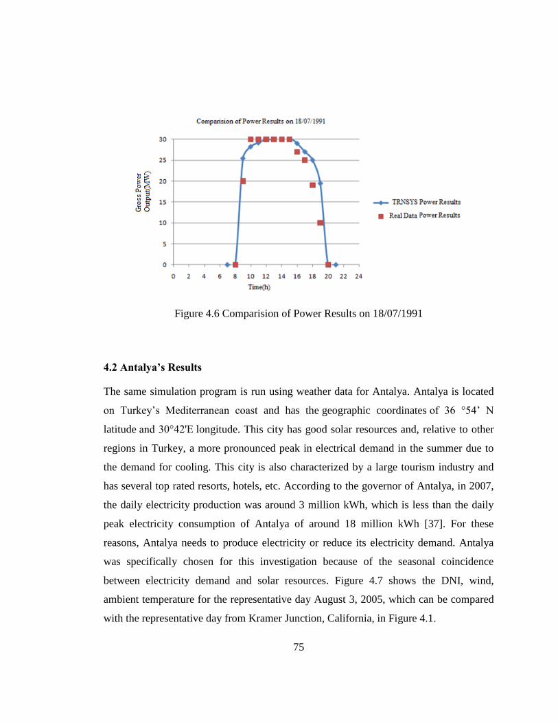
75

Figure 4.6 Comparision of Power Results on 18/07/1991

4.2 Antalya’s Results

The same simulation program is run using weather data for Antalya. Antalya is located

on Turkey’s Mediterranean coast and has the geographic coordinates of 36 °54’ N

latitude and 30°42'E longitude. This city has good solar resources and, relative to other

regions in Turkey, a more pronounced peak in electrical demand in the summer due to

the demand for cooling. This city is also characterized by a large tourism industry and

has several top rated resorts, hotels, etc. According to the governor of Antalya, in 2007,

the daily electricity production was around 3 million kWh, which is less than the daily

peak electricity consumption of Antalya of around 18 million kWh [37]. For these

reasons, Antalya needs to produce electricity or reduce its electricity demand. Antalya

was specifically chosen for this investigation because of the seasonal coincidence

between electricity demand and solar resources. Figure 4.7 shows the DNI, wind,

ambient temperature for the representative day August 3, 2005, which can be compared

with the representative day from Kramer Junction, California, in Figure 4.1.

76

Figure 4.7 Weather Condition of Antalya on August 3, 2005

Figure 4.8 shows the predicted gross power output on August 3, 2005 in Antalya. The

results which are conducted on clear summer day reach nearly 30 MW.

77

Figure 4.8 Predicted Gross Power Output for Antalya for August 3, 2005.

In this study predictions for three different solar conditions are presented for Antalya.

Figure 4.9 shows the typical clear summer week power results. From these predictions it

can be seen that the peak daily power which is generated all week nearly reaches 30

MW. But some variation between days does exist due to differences in cloud cover and

therefore insolation.

78

Figure 4.9 Clear Summer Week Power Results(July, 4-10 2005)

Figure 4.10 shows a typical partly cloudy week power output results for the fall. In

comparing these predictions to those for the clear summer week in Figure 4.9, one can

see significantly larger fluctuations.

Figure 4.10 Cloudy Week Power Output Results(October,18-24 2005)

79

Figure 4.11 shows a typical winter week power output results. The insolation is very low

and the system’s maximum power output is only 15 MW.

Figure 4.11 Winter Week Power Output Result (January,21-28 2005)

Figure 4.12 Clear Summer Week Power Output and DNI (July, 4-10 2005)

80

Figure 4.13 Winter Week Power Output and DNI (January,21-28 2005)

In Figures 4.12 and 4.13 the power output and DNI versus time for a summer and winter

week are presented. These figures are consistent with the trends for DNI and direct

irradiance (DNI x cos(ɸ)) presented in Patnode [16], where the system power output

presented in the present work is substituted for the direct irradiance presented by

Patnode.

Figure 4.14 shows efficiency over a summer day and the system efficiency is nearly

15%, the collector efficiency is approximately 52 %, and cycle efficiency is

approximately 35 %. For winter days efficiency is shown in Figure 4.15. System and

cycle efficiencies decrease and system efficiency is approximately 0.5 %, collector

efficiency is approximately 52 % and cycle efficiency is approximately 0.8 %.

81

Figure 4.14 System, Cycle and Collector Efficiency versus Time Antalya for

August 3, 2005.

Figure 4.15 System, Cycle, Collector Efficiency versus Time Antalya for

January 21, 2005

82

Figure 4.16 is the last graph and it is a summary of the entire study. Average daily power

output of Antalya and Kramer Junction are compared for each month of the year. For

Kramer Junction the maximum daily electricity generated is nearly 290 MWh/day and

these results are obtained in June. For Antalya the maximum daily electricity generated

is 260 MWh/day and these results are obtained in July. According to these results,

Antalya is very suitable place to a construct parabolic trough field.

Figure 4.16 Comparison of Monthly Performance of CSP System in Antalya, Turkey,

and Kramer Junction, California: Average Daily Output, Ratio of Average Daily to

Maximum Average Daily Output, and Ratio of Output in Antalya to Kramer Junction

(KJ).

83

CHAPTER 5

SUMMARY AND CONCLUSIONS

In this study, a model for the solar field and power cycle was created in the TRNSYS

simulation environment using the Solar Thermal Electric Component (STEC) model

library. A model for a 30 MW CSP system was developed based on published data for

an actual system in Kramer Junction, California. The system consists of a collector loop

connected to a power block by a series of heat exchangers. The collector loop consists of

a field of parabolic trough collectors, expansion vessel, pump and heat exchangers to

drive the power block and uses a heat transfer fluid. The series of heat exchangers

connecting the collector loop to the power block are a preheater, steam generator,

superheater, and reheater. In addition to these heat exchangers, the power block consists

of a 2-stage high pressure turbine, 5-stage low pressure turbine, condenser, 5-feed water

heaters, 1-dearator, and 2-pumps. The model’s predictions were benchmarked against

published data for the system in Kramer Junction, California, for a summer day. Good

agreement between the model’s predictions and published data were found, with errors

usually less than 10%. Transient effects such as startup, shutdown, and cloud response

were adequately modeled. Previous work in this area focused on modeling the

performance of the system for a single day operating at Kramer Junction, California. The

present work extends this previous work by presenting and comparing results for annual

simulations for both Kramer Junction and for Antalya, Turkey. Results from

representative summer, fall and winter weeks for Antalya are presented. Major results

are as follows:

For all months of the year, the system in Antalya produces 10% to 50% less

energy than the system in Kramer Junction.

On an annual basis, the system in Antalya produces 30 % less energy than the

system in Kramer Junction.

84

In Antalya the system average daily output is maximum in July and minimum in

December. The ratio of energy produced in December to July is 0.04.

In December the system produces less energy because of high angle of incidence

angle, small projected area, short days and high air mass.

Therefore, while Antalya is known as having good solar resources for Turkey, the

resources are not as good as those in Kramer Junction. Additionally, based on these

results much of the capacity of the 30 MW is not used throughout the year if the system

only relies on solar power without back-up.

85

CHAPTER 6

SUGGESTIONS FOR FUTURE INVESTIGATIONS

This presented study forms a foundation and should be considered as a starting point for

further studies. It is a basic development for a very promising technology which is the

parabolic trough collector system. In the future with required developments and

research, these systems can be more commercially viable. Suggestions to improve on

this present modeling and simulation work are as follows:

The current model does not include storage. Storage can be implemented to

improve the availability of this system and shift electricity production closer to

peak electricity demand.

The current model only includes Therminol VP-1 as a heat transfer fluid. These

models can be improved by implementing water instead of Therminol VP-1 to

model a direct steam generation (DSG) system. As a result, some new important

aspects, such as collector efficiency can be introduced.

The model can be extended to model a parabolic trough plant integrated with a

gas turbine combined-cycle plant, which is a relatively new and promising

concept. This new technology is called an Integrated Solar Combined Cycle

System (ISCCS).

A power tower system can be modeled and its performance compared to that for

a parabolic trough system.

86

The cooling towers for parabolic trough systems typically consume large

quantities of water. The magnitude of this water consumption can be investigated

and compared to local water resources. The impact of using alternate cooling

technologies such as dry cooling towers, which have higher parasitic energy

loses, can be quantified.

Parabolic trough plants are capital-intensive projects and cost reduction should

be investigated and improved.

87

REFERENCES

[1] Aringhoff, R., Brakmann, G., Geyer, M., Teske, S., " Concentrated Solar Thermal

Power-Now" Greenpeace International, ESTIA, IEA SolarPACES Implementing

Agreement, September 2005.

[2] Leitner, A.,"Fuel From the Sky:Solar Power’s Potential for Western Energy Supply",

NREL/SR-550-32160, July 2002.

[3] EC – European Commission" European Research on Concentrated Solar Thermal

Energy, Report EU-20898, 2004.

[4] Hepbaşlı A., Ulgen K., Eke R.,"Solar Energy Application in Turkey.Energy Source,

Part A Utilization and Environmental Effects",DOI:10.1080/00908310490438579

Turkey, 2004.

[5] Kaygusuz, K.,"Prospect of Concentrating Solar Power In Turkey: The Sustainable

Future" Renewable and Sustainable Energy Reviews RSER-1130, Turkey, 2010.

[6] Bilgili, M. E., Yaldiz, O., and Ertekin, C. "A study on the estimation of thermal

efficiency in air heated solar collectors "(in Turkish), Proceedings of Sun Day

Symposium. 25–27 June, Kayseri, Turkey,1999 pp. 275–282.

[7] Stine, W.,B., Geyer, M., "Solar Energy System Design", Last accessed August 13,

2010, http://www.powerfromthesun.net/chapter1/Chapter1.htm.

http://www.powerfromthesun.net/chapter1/Chapter1.htm

88

[8]"Solar Power Towers", Last accessed October 10, 2010,

http://www.solarpaces.org/CSP_Technology/ csp_technology.htm.

[9] " Ptc Technology Assessment Appendix A",NREL CA Solar Benefits, April 21,

2006.

[10]"Solar Dish Systems" Last accessed October 10, 2010


[11]"Solar Parabolic Trough",Last accessed October 10, 2010


[12] Price H, D., Kearney, "Parabolic-Trough Technology Roadmap: A Pathway for

Sustained Commercial Development and Deployment of Parabolic Trough

Technology ", US DOE Report NREL/TE-550-24748, 1999.

[13]"Annual Development of Turkey’s Gross Electricity Generation-Imports-Exports

and Demand (1975-2008),"Turkish Electricity Transmission Co. (TEİAŞ), Ankara,

2008.

[14] "The Distribution of Gross Electricity Generation by Primary Energy Resources

and the Electric Utilities in Turkey," Turkish Electricity Transmission Co. (TEİAŞ),

Ankara, 2007.

[15] "Turkish Electrical Energy 10-Year Generation Capacity Projection," Turkish

Electricity Transmission Co. (TEİAŞ), Ankara, 2009.

[16] Patnode M. A., "Simulation and Performance Evaluation of Parabolic Trough Solar

Power Plants", M.S. Thesis ,University of Wisconsin, Madison,2006.

http://www.solarpaces.org/CSP_Technology/%20csp_technology.htm

http://www.solarpaces.org/CSP_Technology/%20csp_technology.htm

89

[17] Duffie, John A., and Beckman, William A.,"Solar Engineering of Thermal

Processes " 3rd

edition, New York: John Wiley and Sons, Inc., 2006.

[18] Kreider, J.,F, "Solar Energy Applications", Chapter 20, University of Colorado

Boulder, Colorado, 2006..

[19] Dudley, V., Kolb, G.J., Mahoney, A.R., Mancini, T.R., Matthews, C.W., Sloan, M.,

and Kearney, D. Test Results: "SEGS LS-2 Solar Collector", Sandia National

Laboratories, SAND94-1884. December 1994.

[20] Weinstock D., Appelbaum,J., "Optimal Solar Field Design of Stationary

Collectors", DOI:10.1115/1.1756137, ASME, 2004.

[21] Stuetzle, T., Blair, N., Mitchell,J.,W., Beckman, W., "Automatic Control of a 30

MWe SEGS VI Parabolic Trough Plant" Solar Energy Laboratory University of

Wisconsin-Madison.

[22] Stuetzle, T., Blair, "Automatic Control of a 30 MWe SEGS VI Parabolic Trough

Plant", M.S. Thesis, Solar Energy Laboratory University of Wisconsin-Madison,

2002.

[23] Lippke, F., "Simulation of the Part Load Behavior of a 30MWe SEGS Plant",

Prepared for Sandia National Laboratories, Albuquerque, NM, SAND95-1293. June

1995.

90

[24] Manzolini, G., Bellarmino M., Macchi,E.,Silva P., "Solar thermodynamic plants

for cogenerative industrial applications in southern Europe", Renewable Energy 36

(2011),,Elsevier,2010.

[25] Rolim,M. M.,Fraidenraich N.,Tiba C., "Analytic modeling of a solar power plant

with parabolic linear collectors",Solar Energy 83 (2009) 126–133,Elsevier,2008.

[26] Jones, Scott A., Pitz-Paal, R., Schwarzboezl, P., Blair, N., and Cable, R. "TRNSYS

Modeling of the SEGS VI Parabolic Trough Solar Electric Generating System ",

Proceedings of Solar Forum 2001, Washington, D.C. April 2001.

[27] Eduardo I.Ortiz-Rivera, Luisa I. Feliciano-Cruz "Performance Evaluation and

Simulation of a Solar Thermal Power Plant", University of Puerto Rico ,978-1-4244-

2893-9/09, IEEE, 2009.

[28] Price, H., Lüpfert, E., Kearney, D., Zarza, E., Cohen, G., Gee, R., Mahoney, R.,

"Advances in Parabolic Trough Solar Power Technology",DOI: 10.1115/1.1467922,

ASME, 2002.

[29] Geyer, M., Lüpfert,E., Osuna, R., Esteban,A., Schiel, W., Schweitzer,A., Zarza,E.,

Nava,P., Langenkamp,J., Mandelberg,E., "EUROTROUGH - Parabolic Trough

Collector Developed for Cost Efficient Solar Power Generation", Zurich,

Switzerland, September 4-6, 2002.

[30]Parabolic Trough Workshop, "Parabolic Trough Receiver Thermal

Performance",Colorado, March 9, 2007.

[31] Therminol VP1 Vapour Phase Liquid Phase Heat Transfer Fluid,Solutia 1999.

91

[32] "TRNSYS," The University of Wisconsin-Madison Solar Energy Lab, Volume 2,

Madison, 2007.

[33] Schwarzbözl, P.,"A TRNSYS Model Library for Solar Thermal Electric

Components (STEC) ", Reference Manual Release 3.0 Köln, Germany, November

2006.

[34] Incropera, Frank P.,and DeWitt, David P. "Fundamentals of Heat and Mass

Transfer ", 5th edition, New York: John Wiley and Sons, Inc., 2002.

[35] "TRNSYS," The University of Wisconsin-Madison Solar Energy Lab, , Volume 3

Component Library , Madison,2007.

[36] Marion, W.,Urban, K., "Users Manual for TMY2s Typical Meteorogical Years",

NREL, June, 1995.

[37] Baş, K., Antalya'da Yeni Enerji Yatırımlarına Ihtiyaç Duyuluyor, Last accessed

May 25, 2010, http://www.zaman.com.tr/haber.do?haberno=573763 (in

Turkish).

[38] Usta, Y.,Çağlar A.,Akkuş,K.,Yılmaz Y.,Taştepe E.,Yüksel, Y.,Öztürk, İ.,Design of

Parabolic Collector and Vacuum Tube, METU Ankara, January 2008.

92

APPENDIX A

PARABOLIC TROUGH COLLECTOR DESIGN TOOL USING VISUAL BASIC

A design program was developed by several students from Middle East Technical

University [38]. The program is designed to calculate of the amount of heat transmitted

from the collector and the transferred heat to the heat transfer fluid. According to the

detailed design methodology explained in the Theory section below, an algorithm has

been formed.

The program consists of two parts. The first part calculates the energy from the collector

field and the second part uses this energy and calculates the efficiency of the vacuum

tube, energy loss, and outlet temperature of fluid.

The program consists of a user friendly interface. After starting the program, a menu

comes to the screen. In this screen, there are 3 parts: collector geometry, reflective

coating of the collector, city and calculation period. In the first part, the important

variables that are to be determined by the user are listed as shown in Figures A.1-A3

Some of these are given as a list among which the variable is selected but the others are

not.

93

Figure A.1 Design Parameters of Parabolic Trough Collector Field

Rim angle and a

& f values

should be in

accaptable range

94

Figure A.2 Selection of City, Months and Coating of the Collector

95

Figure A.3 Result Window

The second part of the program design calculates efficiency, outlet temperature of the

fluid, and heat losses of the vacuum tube. The user can change the values assigned in

these boxes. In the output section of the program, energy obtained from the tube, energy

loss, outlet temperature of the fluid and efficiency of the tube are given.

In addition to all explained features of the program above, there are some safety

margins. These margins enable the user to use the program within some definite and

reasonable limits. Also possible errors due to unrealistic inputs are avoided. Moreover

with the help of the warnings in the program, it is much easier to utilize the program.

Firstly, if the users attempts to execute the program without entering one of the

96

parameters in the inputs section, the program warns the user by providing the error

message below shown in Figure A.4 (the message changes according to the parameter

that is not defined).

Figure A. 4 Error Message

Secondly, the program is designed to serve a list of fluids. The fluids are assumed to

operate in the liquid form. Thus the phase changes and the heat transfer in two phases

are excluded. With this respect, if the energy of the system is high enough to change the

phase of the given fluid, the program warns the user and asks him for defining new

parameters. The error message related to this option is given below in Figure A.5:

97

Figure A. 5 Vacuum Tube Datas

Another important limit check is about the diameter of the tube and the absorber

diameter. Since it is not geometrically possible that the absorber diameter is greater than

the tube diameter, when the user defines wrong values in these boxes, the program

warns the user with the following error message shown in Figure A.6:

98

The last limit check is about the efficiency of the program. In some circumstances of

low energy input, the energy output may be very small. Because of the assumptions used

in the calculations, the calculated efficiency may be very small. In these types of

circumstances, the program warns the user and prompts him to enter more reasonable

values.

Figure A.6 Chosing Absorber Diameter

99

APPENDIX B

TMY2 DATA AND FORMAT

For each location, a TMY2 file contains values for one year of hourly solar radiation,

illuminance, and meteorological data. The file header contains the, city, state, time zone,

latitude, longitude, and elevation. The location and description of these header elements

are given in Table 3-1. Each hourly record begins with the year from which the typical

month was chosen, followed by the month, day, and hour information in field positions

[36].

Fig

ure

B.

1 S

ample

fil

e h

eader

and d

ata

in t

he

TM

Y2 f

orm

at f

or

Januar

y 1

[36]

100

101

Table B. 1 Header Elements in the TMY2 Format[36]

Table B. 2 Data Elements in the TMY2 Format[36]

102

Table B. 3 Data Elements in the TMY2 Format (Continued)

103

APPENDIX C

SAMPLE TRNSYS INPUT (DECK) FILE

VERSION 16.1

***************************************************************************

****

*** TRNSYS input file (deck) generated by TrnsysStudio

***

*** If you edit this file, use the File/Import TRNSYS Input File function in

*** TrnsysStudio to update the project.

***

*** If you have problems, questions or suggestions please contact your local

*** TRNSYS distributor or mailto:[email protected]

***

***************************************************************************

****

***************************************************************************

****

*** Units

***************************************************************************

****

***************************************************************************

****

104

*** Control cards

***************************************************************************

****

* START, STOP and STEP

CONSTANTS 3

START=4751

STOP=4774

STEP=1

* User defined CONSTANTS

SIMULATION START STOP STEP ! Start time End time Time step

TOLERANCES 0.001 0.001 ! Integration Convergence

LIMITS 30 30 30 ! Max iterations Max warnings Trace limit

DFQ 1 ! TRNSYS numerical integration solver method

WIDTH 80 ! TRNSYS output file width, number of characters

LIST ! NOLIST statement

! MAP statement

SOLVER 0 1 1 ! Solver statement Minimum relaxation factor

Maximum relaxation factor

NAN_CHECK 0 ! Nan DEBUG statement

OVERWRITE_CHECK 0 ! Overwrite DEBUG statement

TIME_REPORT 0 ! disable time report

EQSOLVER 0 ! EQUATION SOLVER statement

* Model "Superheater" (Type 315)

*

UNIT 2 TYPE 315 Superheater

*$UNIT_NAME Superheater

*$MODEL .\STEC Library\Rankine\Steamgen\Eco_sh.tmf

*$POSITION 115 247

105

*$LAYER Main #

PARAMETERS 6

2 ! 1 Counter flow mode

1051199.972153 ! 2 Overall heat transfer coefficient of exchanger

0 ! 3 Reference press loss cold side

139836.593628 ! 4 Reference cold side flow

0 ! 5 power law exp for UA

0 ! 6 power law exp for DP

INPUTS 7

0,0 ! [unconnected] Hot side inlet temperature

34,3 ! Splitter:outlet flow rate 2 ->Hot side flow rate

3,3 ! Evaporator(steam generator):Cold side outlet temperature ->Cold side inlet

temperature

3,7 ! Evaporator(steam generator):Cold side outlet flow rate ->Cold side flow rate

3,5 ! Evaporator(steam generator):Cold side outlet quality ->Cold side quality

33,2 ! X2H2:steam pressure ->cold side outlet pressure

0,0 ! [unconnected] hot side spedific heat

*** INITIAL INPUT VALUES

390.56 1427039.978027 313.89 140288.406372 1 100 2.59

*------------------------------------------------------------------------------

* Model "Evaporator(steam generator)" (Type 316)

*

UNIT 3 TYPE 316 Evaporator(steam generator)

*$UNIT_NAME Evaporator(steam generator)

*$MODEL .\STEC Library\Rankine\Steamgen\Evaporator.tmf

*$POSITION 116 345

*$LAYER Main #

PARAMETERS 6

7383599.804401 ! 1 overall heat transfer factor

0.0 ! 2 blowdown fraction

106

0 ! 3 reference pressure loss

139836.593628 ! 4 reference flow rate

0 ! 5 power lax exp for UA

0 ! 6 power law exp for dp

INPUTS 6

2,1 ! Superheater:Hot-side outlet temperature ->Hot side inlet temperature

2,2 ! Superheater:Hot-side flow rate ->Hot side flow rate

4,3 ! Economizer(preheater):Cold-side outlet temperature ->Cold side inlet

temperature

2,8 ! Superheater:Cold Side Inlet pressure ->Cold side outlet pressure

4,7 ! Economizer(preheater):Cold side Outlet quality ->Cold side inlet quality

0,0 ! [unconnected] Hot side specific heat capacity


377.22 1243763.964844 313.89 103.42 0.0 2.54

*------------------------------------------------------------------------------

* Model "Economizer(preheater)" (Type 315)

*

UNIT 4 TYPE 315 Economizer(preheater)

*$UNIT_NAME Economizer(preheater)


*$POSITION 110 449

*$LAYER Main #

PARAMETERS 6







INPUTS 7

107

3,1 ! Evaporator(steam generator):Hot side outlet temperture ->Hot side inlet

temperature

3,2 ! Evaporator(steam generator):Hot side outlet flow rate ->Hot side flow rate

28,2 ! FWH 5:Cold side outlet temperture ->Cold side inlet temperature

28,3 ! FWH 5:Cold side outlet flow rate ->Cold side flow rate

0,0 ! [unconnected] Cold side quality

3,4 ! Evaporator(steam generator):Cold side inlet pressure ->cold side outlet

pressure



317.78 1243763.964844 234.83 140288.406372 0.0 103.42 2.36

*------------------------------------------------------------------------------

* Model "hp stage 1" (Type 318)

*

UNIT 5 TYPE 318 hp stage 1

*$UNIT_NAME hp stage 1

*$MODEL .\STEC Library\Rankine\Turbine\Stage.tmf

*$POSITION 174 368

*$LAYER Main #

PARAMETERS 8

100 ! 1 design inlet pressure

33.61 ! 2 design outlet pressure

139109.394836 ! 3 design flow rate

0.8376 ! 4 design inner efficiency

0.95 ! 5 generator efficiency

0.0 ! 6 coef. for inner eff eq

0.0 ! 7 b coeff for inner eff

0.0 ! 8 c coeff for inner eff

INPUTS 4

8,4 ! S-split-1:inlet pressure ->Turbine outlet pressure

108

33,3 ! X2H2:steam flow rate ->Turbine inlet flow rate

33,1 ! X2H2:steam enthalpy ->Turbine inlet enthalpy

0,0 ! [unconnected] Bypass indicator


33.61 139109.394836 3005 1

*------------------------------------------------------------------------------

* Model "hp stage 2" (Type 318)

*

UNIT 6 TYPE 318 hp stage 2

*$UNIT_NAME hp stage 2


*$POSITION 420 368

*$LAYER Main #

PARAMETERS 8

33.61 ! 1 design inlet pressure








INPUTS 4

7,4 ! S-split-2:inlet pressure ->Turbine outlet pressure

8,3 ! S-split-1:outlet flow rate 2 ->Turbine inlet flow rate

8,6 ! S-split-1:outlet enthalpy 2 ->Turbine inlet enthalpy



18.58 128637.364197 2807 1

*------------------------------------------------------------------------------

109

* Model "S-split-2" (Type 389)

*

UNIT 7 TYPE 389 S-split-2

*$UNIT_NAME S-split-2

*$MODEL .\STEC Library\Rankine\Turbine\S-split.tmf

*$POSITION 544 368

*$LAYER Main #

INPUTS 4

27,1 ! FWH4:Demanded hot inlet flow rate ->Demanded Flow Out 1

6,2 ! hp stage 2:turbine outlet flowrate ->inlet flow rate

9,8 ! Reheater:Cold Side Inlet pressure ->outlet pressure 2

6,3 ! hp stage 2:turbine outlet enthalpy ->inlet enthalpy


10083.239937 128637.364197 18.58 2807

*------------------------------------------------------------------------------

* Model "S-split-1" (Type 389)

*

UNIT 8 TYPE 389 S-split-1

*$UNIT_NAME S-split-1


*$POSITION 304 368

*$LAYER Main #

INPUTS 4

28,1 ! FWH 5:Demanded hot inlet flow rate ->Demanded Flow Out 1

5,2 ! hp stage 1:turbine outlet flowrate ->inlet flow rate

6,1 ! hp stage 2:turbine inlet pressure ->outlet pressure 2

5,3 ! hp stage 1:turbine outlet enthalpy ->inlet enthalpy


110

10551.95961 139109.394836 33.61 3005

*------------------------------------------------------------------------------

* Model "Reheater" (Type 315)

*

UNIT 9 TYPE 315 Reheater

*$UNIT_NAME Reheater


*$POSITION 619 249

*$LAYER Main #

PARAMETERS 6







INPUTS 7

0,0 ! [unconnected] Hot side inlet temperature

34,1 ! Splitter:outlet flow rate 1 ->Hot side flow rate

0,0 ! [unconnected] Cold side inlet temperature

7,3 ! S-split-2:outlet flow rate 2 ->Cold side flow rate

0,0 ! [unconnected] Cold side quality

37,2 ! X2H2-2:steam pressure ->cold side outlet pressure



390.56 183254.38385 208.67 118929.597473 1 17.10 2.59

*------------------------------------------------------------------------------

* Model "lp stage 1" (Type 318)

*

111

UNIT 10 TYPE 318 lp stage 1

*$UNIT_NAME lp stage 1


*$POSITION 36 294

*$LAYER Main #

PARAMETERS 8









INPUTS 4

15,4 ! lp split 1:inlet pressure ->Turbine outlet pressure

37,3 ! X2H2-2:steam flow rate ->Turbine inlet flow rate

37,1 ! X2H2-2:steam enthalpy ->Turbine inlet enthalpy



7.98 118104.483032 3190 1

*------------------------------------------------------------------------------


*




*$POSITION 249 294

*$LAYER Main #

112

PARAMETERS 8









INPUTS 4


15,3 ! lp split 1:outlet flow rate 2 ->Turbine inlet flow rate

15,6 ! lp split 1:outlet enthalpy 2 ->Turbine inlet enthalpy



2.73 110856.960297 3016 1

*------------------------------------------------------------------------------


*




*$POSITION 452 294

*$LAYER Main #

PARAMETERS 8






113




INPUTS 4






0.96 104516.640472 2798 1

*------------------------------------------------------------------------------

* Model "lp stage 4." (Type 318)

*

UNIT 13 TYPE 318 lp stage 4.

*$UNIT_NAME lp stage 4.


*$POSITION 677 294

*$LAYER Main #

PARAMETERS 8









INPUTS 4



114




0.29 98696.880341 2624 1

*------------------------------------------------------------------------------


*




*$POSITION 879 294

*$LAYER Main #

PARAMETERS 8









INPUTS 4

19,2 ! Condenser:Condensing pressure ->Turbine outlet pressure





0.08 95802.113342 2325 1

*------------------------------------------------------------------------------

115

* Model "lp split 1" (Type 389)

*

UNIT 15 TYPE 389 lp split 1

*$UNIT_NAME lp split 1


*$POSITION 150 294

*$LAYER Main #

INPUTS 4

22,2 ! Deaerator:required steam flow rate ->Demanded Flow Out 1

10,2 ! lp stage 1:turbine outlet flowrate ->inlet flow rate

11,1 ! lp stage 2:turbine inlet pressure ->outlet pressure 2

10,3 ! lp stage 1:turbine outlet enthalpy ->inlet enthalpy


7307.999897 118104.483032 7.97 3190

*------------------------------------------------------------------------------


*




*$POSITION 342 294

*$LAYER Main #

INPUTS 4






6335.999966 110856.960297 2.72 3016

116

*------------------------------------------------------------------------------


*




*$POSITION 566 294

*$LAYER Main #

INPUTS 4



13,1 ! lp stage 4.:turbine inlet pressure ->outlet pressure 2



5832.000017 104516.640472 0.96 2798

*------------------------------------------------------------------------------


*




*$POSITION 780 294

*$LAYER Main #

INPUTS 4


13,2 ! lp stage 4.:turbine outlet flowrate ->inlet flow rate


13,3 ! lp stage 4.:turbine outlet enthalpy ->inlet enthalpy

117


2844.000077 98696.880341 0.28 2624

*------------------------------------------------------------------------------

* Model "Condenser" (Type 383)

*

UNIT 19 TYPE 383 Condenser

*$UNIT_NAME Condenser

*$MODEL .\STEC Library\Rankine\Condenser\Condens.tmf

*$POSITION 930 249

*$LAYER Main #

PARAMETERS 2

5.0 ! 1 dT Cool water out+condensing temp

5.0 ! 2 temp increase in cool. water

INPUTS 6

0,0 ! [unconnected] Cooling water inlet temp

14,3 ! lp stage 5:turbine outlet enthalpy ->steam enthalpy inlet

14,2 ! lp stage 5:turbine outlet flowrate ->steam mass flow rate

24,5 ! FWH1:Hot side outlet flow rate ->Condensate inlet flow rate

0,0 ! [unconnected] Condensate inlet temperture

24,6 ! FWH1:Hot side outlet quality ->Condensate inlet quality


25.5 2348.1 26.482001 16153.560448 52.889 0

*------------------------------------------------------------------------------

* Model "Condensate Pump" (Type 300)

*

UNIT 20 TYPE 300 Condensate Pump

*$UNIT_NAME Condensate Pump

*$MODEL .\STEC Library\Ste\Utility\Saltpu_1.tmf

118

*$POSITION 940 378

*$LAYER Main #

PARAMETERS 5

111488.399506 ! 1 Maximum flow rate

4.19 ! 2 Fluid specific heat

683999.98188 ! 3 Maximum power

0.0 ! 4 Conversion coefficient

0.5 ! 5 Power coefficient

INPUTS 3

19,1 ! Condenser:Condesing Temperature ->Inlet fluid temperature

19,6 ! Condenser:Condesate flow rate ->Inlet mass flow rate

0,0 ! [unconnected] desired mass flow rate


41.439 111488.399506 111488.399506

*------------------------------------------------------------------------------

* Model "FW pump" (Type 300)

*

UNIT 21 TYPE 300 FW pump

*$UNIT_NAME FW pump


*$POSITION 519 474

*$LAYER Main #

PARAMETERS 5



3167999.916077 ! 3 Maximum power



INPUTS 3

22,1 ! Deaerator:Feed water out temp ->Inlet fluid temperature

119

22,3 ! Deaerator:Feed Water out flow rate ->Inlet mass flow rate

3,6 ! Evaporator(steam generator):Cold side flow rate demand ->desired mass flow

rate


166.89 140288.406372 140288.406372

*------------------------------------------------------------------------------

* Model "Deaerator" (Type 384)

*

UNIT 22 TYPE 384 Deaerator

*$UNIT_NAME Deaerator

*$MODEL .\STEC Library\Rankine\preheating\Deaerator.tmf

*$POSITION 623 473

*$LAYER Main #

INPUTS 8

26,2 ! FWH3:Cold side outlet temperture ->Feed Water in tmp

26,3 ! FWH3:Cold side outlet flow rate ->Feed Water flow rate

15,5 ! lp split 1:outlet enthalpy 1 ->steam inlet enthalpy

15,2 ! lp split 1: outlet pressure 1 ->steam inlet pressure

0,0 ! [unconnected] condesate inlet temperture

27,5 ! FWH4:Hot side outlet flow rate ->Condesate inlet flow rate


0,0 ! [unconnected] Dearator on/off


126.72 111722.401428 3029.4 7.33 179.17 20628.000069 0.0 1.0

*------------------------------------------------------------------------------

* Model "FWH1" (Type 317)

*

UNIT 24 TYPE 317 FWH1

120

*$UNIT_NAME FWH1

*$MODEL .\STEC Library\Rankine\preheating\Preheater.tmf

*$POSITION 939 473

*$LAYER Main #

PARAMETERS 4

4.18 ! 1 cold fluid spef. heat capacity


111708.002472 ! 3 cold sid ref flow rate


INPUTS 8

18,5 ! lp split 4:outlet enthalpy 1 ->Hot side inlet enthalpy

18,2 ! lp split 4: outlet pressure 1 ->Hot side inlet pressure

20,1 ! Condensate Pump:Outlet fluid temperature ->Cold side inlet temperature

20,2 ! Condensate Pump:Outlet flow rate ->Cold side inlet flow rate

0,0 ! [unconnected] Condensate inlet temperature



0,0 ! [unconnected] on/off


2528.1 0.2797 41.61 111708.002472 74.722 12200.760269 0 1

*------------------------------------------------------------------------------


*


*$UNIT_NAME FWH2


*$POSITION 814 473

*$LAYER Main #

PARAMETERS 4


121




INPUTS 8



24,2 ! FWH1:Cold side outlet temperture ->Cold side inlet temperature

24,3 ! FWH1:Cold side outlet flow rate ->Cold side inlet flow rate






2624.4 0.9625 64.722 111708.002472 105.06 6367.320013 0 1

*------------------------------------------------------------------------------


*


*$UNIT_NAME FWH3


*$POSITION 712 475

*$LAYER Main #

PARAMETERS 4





INPUTS 8



122




0,0 ! [unconnected] Condensate inlet flow rate

0,0 ! [unconnected] Condensate inlet quality



2798.2 2.7276 95.111 111708.002472 105.06 0 0 1

*------------------------------------------------------------------------------


*


*$UNIT_NAME FWH4


*$POSITION 392 473

*$LAYER Main #

PARAMETERS 4





INPUTS 8

7,5 ! S-split-2:outlet enthalpy 1 ->Hot side inlet enthalpy

7,4 ! S-split-2:inlet pressure ->Hot side inlet pressure

21,1 ! FW pump:Outlet fluid temperature ->Cold side inlet temperature

21,2 ! FW pump:Outlet flow rate ->Cold side inlet flow rate


28,5 ! FWH 5:Hot side outlet flow rate ->Condensate inlet flow rate

28,6 ! FWH 5:Hot side outlet quality ->Condensate inlet quality


123


2709.6 18.581 169.22 140288.406372 213.67 10551.95961 0 1

*------------------------------------------------------------------------------

* Model "FWH 5" (Type 317)

*

UNIT 28 TYPE 317 FWH 5

*$UNIT_NAME FWH 5


*$POSITION 296 473

*$LAYER Main #

PARAMETERS 4





INPUTS 8

8,5 ! S-split-1:outlet enthalpy 1 ->Hot side inlet enthalpy

8,2 ! S-split-1: outlet pressure 1 ->Hot side inlet pressure




0,0 ! [unconnected] Condensate inlet flow rate

0,0 ! [unconnected] Condensate inlet quality



2807 33.612 203.61 140288.406372 213.67 0 0 1

*------------------------------------------------------------------------------

* Model "Trough-2" (Type 396)

*

124

UNIT 29 TYPE 396 Trough-2

*$UNIT_NAME Trough-2

*$MODEL .\STEC Library\STE\Trough\Trough.tmf

*$POSITION 462 59

*$LAYER Main #

PARAMETERS 22

73.6 ! 1 A - Loss coef.

-0.0042 ! 2 B - Loss coef.

7.40 ! 3 C - Loss coef.

0 ! 4 Cw- Loss coef.

-0.096 ! 5 D - Loss coef.

0.94 ! 6 Clean Reflectivity

0.0 ! 7 Broken Mirror Fraction

47 ! 8 Length of SCA

5 ! 9 Aperature Width of SCA

5 ! 10 Focal Length of SCA

15 ! 11 Rowspacing

182000 ! 12 Total Field Area

5759999.847412 ! 13 Pump Max Power

1427039.978027 ! 14 Pump Max Flow Rate

1.308 ! 15 Pump Power Coeff. 1

4.28E-3 ! 16 Pump Power Coeff. 2

1.99E-5 ! 17 Pump Power Coeff. 3

0 ! 18 Tank Heat Loss Rate at 275 C

20 ! 19 Piping Heat Loss/Area at 343C

0.86 ! 20 Field Tracking Parasitics/Area

11250 ! 21 Stow Energy for Each m2 Field Area

5 ! 22 Wind Speed Limit for Tracking

INPUTS 14

0,0 ! [unconnected] Demanded Outlet Temperature

36,1 ! HTF Pump:Outlet fluid temperature ->Inlet Temperature Solar Field

125

0,0 ! [unconnected] Cleanliness Solar Field

0,0 ! [unconnected] Specific Heat HTF

32,11 ! Weather Data:solar azimuth angle ->Sun Azimuth

32,10 ! Weather Data:solar zenith angle ->Sun Zenith

32,19 ! Weather Data:beam radiation on tilted surface ->DNI- Direct Normal

Radiation

32,3 ! Weather Data:wind velocity ->Wind Speed

32,1 ! Weather Data:Ambient temperature ->Ambient Temperature

0,0 ! [unconnected] Tracking Fraction of Field

0,0 ! [unconnected] Available Fraction of Field

0,0 ! [unconnected] Night Flow Ratio (min Flow)

0,0 ! [unconnected] Rampdown Time

0,0 ! [unconnected] Rampdown Ratio


390.56 297.78 0.95 2.59 0 0 900 0 30 1.0 1.0 0.1 1 1

*------------------------------------------------------------------------------

* Model "Expansion Vessel" (Type 4)

*

UNIT 30 TYPE 4 Expansion Vessel

*$UNIT_NAME Expansion Vessel

*$MODEL .\Thermal Storage\Stratified Storage Tank\Fixed Inlets\Uniform

Losses\Type4a.tmf

*$POSITION 632 61

*$LAYER Main #

PARAMETERS 20

1 ! 1 Fixed inlet positions

287 ! 2 Tank volume


704 ! 4 Fluid density

0 ! 5 Tank loss coefficient

126

0.05 ! 6 Height of node

1 ! 7 Auxiliary heater mode

1 ! 8 Node containing heating element 1

1 ! 9 Node containing thermostat 1

0 ! 10 Set point temperature for element 1

5.0 ! 11 Deadband for heating element 1

16200.0 ! 12 Maximum heating rate of element 1

1 ! 13 Node containing heating element 2

1 ! 14 Node containing thermostat 2

0 ! 15 Set point temperature for element 2

5.0 ! 16 Deadband for heating element 2

16200 ! 17 Maximum heating rate of element 2

0.0 ! 18 Not used (Flue UA)

20.0 ! 19 Not used (Tflue)

257 ! 20 Boiling point

INPUTS 7

29,2 ! Trough-2:Outlet Temperature Solar Field ->Hot-side temperature

29,1 ! Trough-2:Flow Rate Solar Field ->Hot-side flowrate

0,0 ! [unconnected] Cold-side temperature

0,0 ! [unconnected] Cold-side flowrate

0,0 ! [unconnected] Environment temperature

0,0 ! [unconnected] Control signal for element-1

0,0 ! [unconnected] Control signal for element-2


390.56 1427039.978027 297 0 30 0.0 0.0

DERIVATIVES 1

0 ! 1 Initial temperature of node

*------------------------------------------------------------------------------

* Model "Weather Data" (Type 109)

*

127

UNIT 32 TYPE 109 Weather Data

*$UNIT_NAME Weather Data

*$MODEL .\Weather Data Reading and Processing\Standard Format\TMY2\Type109-

TMY2.tmf

*$POSITION 329 40

*$LAYER Main #

PARAMETERS 4

2 ! 1 Data Reader Mode

32 ! 2 Logical unit

4 ! 3 Sky model for diffuse radiation

4 ! 4 Tracking mode

INPUTS 3

0,0 ! [unconnected] Ground reflectance

0,0 ! [unconnected] Slope of surface

0,0 ! [unconnected] Azimuth of surface


0.2 0.0 0.0

*** External files

ASSIGN "C:\Users\acer\Desktop\3 değişken+hava.txt" 32

*|? Weather data file |1000

*------------------------------------------------------------------------------

* Model "X2H2" (Type 391)

*

UNIT 33 TYPE 391 X2H2

*$UNIT_NAME X2H2

*$MODEL .\STEC Library\Rankine\Utility\X2H.TMF

*$POSITION 333 249

*$LAYER Main #

INPUTS 4

2,3 ! Superheater:Cold-side outlet temperature ->Steam temperture

128

5,1 ! hp stage 1:turbine inlet pressure ->Steam pressure

2,7 ! Superheater:Cold side Outlet quality ->Steam quality

2,4 ! Superheater:Cold-side flow rate ->Steam flow rate


371 100 1 140288.406372

*------------------------------------------------------------------------------

* Model "Splitter" (Type 389)

*

UNIT 34 TYPE 389 Splitter

*$UNIT_NAME Splitter


*$POSITION 573 155

*$LAYER Main #

INPUTS 4

0,0 ! [unconnected] Demanded Flow Out 1

30,2 ! Expansion Vessel:Flowrate to heat source ->inlet flow rate

0,0 ! [unconnected] outlet pressure 2

0,0 ! [unconnected] inlet enthalpy


183254.38385 1427039.978027 23.167 0

*------------------------------------------------------------------------------

* Model "Mixer" (Type 330)

*

UNIT 35 TYPE 330 Mixer

*$UNIT_NAME Mixer

*$MODEL .\STEC Library\Rankine\Turbine\S-MIX.tmf

*$POSITION 251 155

*$LAYER Main #

129

INPUTS 5

9,2 ! Reheater:Hot-side flow rate ->Inlet Flowrate 1

0,0 ! [unconnected] Inlet Enthalpy 1

4,2 ! Economizer(preheater):Hot-side flow rate ->Inlet Flowrate 2

0,0 ! [unconnected] Inlet Enthalpy 2

0,0 ! [unconnected] Outlet Pressure


183254.38385 0 1243763.964844 0 21

*------------------------------------------------------------------------------

* Model "HTF Pump" (Type 300)

*

UNIT 36 TYPE 300 HTF Pump

*$UNIT_NAME HTF Pump


*$POSITION 362 154

*$LAYER Main #

PARAMETERS 5



5759999.847412 ! 3 Maximum power



INPUTS 3

0,0 ! [unconnected] Inlet fluid temperature

35,1 ! Mixer:Outlet Flowrate 1 ->Inlet mass flow rate

0,0 ! [unconnected] desired mass flow rate


297.78 1427039.978027 1427039.978027

*------------------------------------------------------------------------------

130

* Model "X2H2-2" (Type 391)

*

UNIT 37 TYPE 391 X2H2-2

*$UNIT_NAME X2H2-2

*$MODEL .\STEC Library\Rankine\Utility\X2H.TMF

*$POSITION 694 251

*$LAYER Main #

INPUTS 4

9,3 ! Reheater:Cold-side outlet temperature ->Steam temperture

10,1 ! lp stage 1:turbine inlet pressure ->Steam pressure

9,7 ! Reheater:Cold side Outlet quality ->Steam quality

9,4 ! Reheater:Cold-side flow rate ->Steam flow rate


371 17.099 1 118929.597473

*------------------------------------------------------------------------------

END

theoretical and experimental investigation of a ... · the commercial software trnsys and the solar...

Documents