1

A TRNSYS Model Libraryfor Solar Thermal Electric Components

(STEC)

A Reference ManualRelease 2.2

September 2002

Peter SchwarzbözlUlrich Eiden

Robert Pitz-PaalDeutsches Zentrum

für Luft und Raumfahrt e.V. (DLR)D-51170 Köln, Germany

Scott JonesSandia National Laboratories

Albuquerque, NM, USA

2

3

Preface

Release 1.0

This is the first version of the Reference Manual of the TRNSYS Model Library of Solar Thermal

Electric Components (STEC). This document gives an overview on the intention of this library, its

theoretical background, and on the structure of the library. It also presents some sample applications

to demonstrate how the components can be set-up in an assembly. The appendix gives technical

information on the hardware and software system requirements, how to install the library, as well as a

complete documentation on all models distributed with the STEC library. This document does not

intend to replace the software description of TRNSYS and its user interface IISibat. Applicants of the

STEC library should have a basic understanding of TRNSYS and on the IISibat Interface.

TRNSYS and the STEC Library are tools which help technical experts to analyse the performance of

a solar thermal power system in detail. On the basis of models which are set-up by these expert users,

the TRNSYS tool TRNSED can be used to convert this model into a black box software program, that

is easy to operate by non-technical experts for performing parameter variations, system studies, or

comparisons with actual plant output. No software or license need to be purchased to use a TRNSED

model. However, in order to develop or operate models in TRNSYS using the STEC model library,

the user must have a valid software license of the TRNSYS code and the IISibat user interface. The

STEC library itself is distributed for free and without any warranty Please ask for a copy (Robert.Pitz-

Paal@dlr.de), which will be send to you by email. Comments and bug reports are highly appreciated.

Also modifications of the code and the development of the new STEC models (e.g. Dish concentrator,

receiver, Stirling engine, improved central receiver models...) are of high interest and a copy of the

code (send by email) would be highly appreciated and will be considered to be included into the next

STEC release.

October 1998 Robert Pitz-Paal

Scott Jones

4

5

Release 2.0

The models of the STEC library are permanently used and improved since the first release in 1998.

The STEC library was upgraded for compatibility with the new TRNSYS 15 and Iisibat3 by former

TRNSYS engineer Nathan Blair from University of Wisconsin in summer 2000. Few changes have

been made to the steam generation models of the Rankine sublibrary. In the STE sublibrary a new

trough model was added with improved modelling of startup and shutdown of parabolic trough fields

(Type196). The former Type96 is now called ‘oldtrough’ and has the new type number 197. Some

other new models were added, mostly for improved modelling of solar cycles. The model library for

gas turbine cycles, created by colleagues from the IVTAN institute in Moscow (Russia), was adapted

to the standard TRNSYS modelling approach and now belongs to the STEC library as the Brayton

sublibrary.

To ensure STEC library users are committed to contribute their new developments to the library in

exchange for using it for free, a formal SolarPACES agreement has been created (see next page). It

has to be signed before receiving the new release 2.0 .

This document is an update of the SolarPACES Technical Report No.III – 4/98 (Reference Manual

for the STEC library release 1.0 from October 1998). It was revised and adapted according to the new

TRNSYS 15/ Iisibat3 features. The explanation of a new example project was added (see Example 3

in Chapter 5). The former Appendix A3 containing the model headers as documentation is no longer

maintained and therefore not included in this document. Users are advised to refer to the Iisibat

proforma for model documentation.

March 2001 Robert Pitz-Paal

Peter Schwarzbözl

6

Release 2.2

One year and a half have past since the last release of the TRNSYS STEC model library and quite a

lot of new developments have been made since then. Therefore, this new release contains more than

20 new types and a couple of new property routines.

The Rankine sublibrary has been restructured and now contains only one – the latest – version for

each component. Two new types have been added by our US-colleagues for improved turbine control

in start-up and shut-down procedures. The biggest improvements have been made to the Brayton

sublibrary, which has now two new sections – ‘CIEMAT’ and ‘DLR’ – containing each a complete

set of gas turbine cycle components. They have different advantages and disadvantages and users

should decide themselves which modelling approach suits best for their purposes. The Solar Thermal

sublibrary has a new trough subsection called ‘CIEMAT’, containing a couple of new types with a

more sophisticated modelling approach for parabolic trough collectors. Further on, two new tower

receiver models have been added to this sublibrary. All the other models have been revised and

several bugs could be fixed. Model documentation was revised as well and is maintained on two

levels: Basic descriptions of each type can be found in the corresponding Iisibat proforma.

Additionally, if available, more detailed documentation about important components or complicated

models was added to this Reference Guide. For further questions the user should try to contact the

author / editor of the type directly.

The DLR, as the official ‘keeper’ of the STEC model library, is collecting new developments from the

users, adding documentation and example projects and putting together new releases every one or two

years to distribute for free among registered SolarPACES members. Therefore, the DLR and the other

authors of the STEC models can not be made responsible for the functionality of this software and the

results obtained while using it. Furthermore, as the DLR has no extra budget for the STEC activity,

the support of users has to be limited to a small level.

Last but not least the authors wish to express their gratefulness to the users, who contributed own

models to the library or gave important remarks to improve the existing ones, and appeal to the others

to share their developments with all the colleagues of this user group.

September 2002 Peter Schwarzbözl

Ulrich Eiden

German Aerospace Center (DLR)

7

TRNSYS STEC User Agreement for SolarPACES Members

The model library of solar thermal electric components (STEC) for the simulation environmentTRNSYS is under development by SolarPACES members in projects with substantial public financialsupport and shall therefore be distributed for free.This open status shall be maintained. However, to ensure STEC library users are committed tocontribute their new developments to the library in exchange for use of the library, this formalagreement has been created. According to the discussions at the SolarPACES Workshop meeting inSeptember 2000, the following rules are laid down:

1. The STEC library shall be distributed solely by one responsible entity (currently: DLRCologne). Distribution by users to a third party is not allowed.

2. Component models are distributed only within the SolarPACES community, includingsource code, Iisibat proforma, and comprehensive documentation.

3. The sharing of system models (multiple components connected together) is encouraged, butnot required.

4. In publications where STEC models or results of STEC simulations are used the library hasto be referenced.

5. Users commit themselves to provide their new, documented component models to the STECLibrary within eight weeks of the public presentation of results obtained with their modelsin combination with the STEC Library. Exceptions are granted with prior approval fordevelopments that are part of contracted confidential work completed with partially privatefunding.

As legal representative of our organisation I confirm our commitment to use this library only incompliance with the rules stated above.

Signature: ..................................................................... Date: .........................

Name: ................................................................................................................

Organisation: ...................................................................................................

Address: ...........................................................................................................

Phone/Fax/E-mail: ...........................................................................................

In order to receive the new library release (adapted to TRNSYS 15) please let this form be signed byyour legal representative and fax to:

Deutsches Zentrum für Luft- und Raumfahrt e.V.Institut für Technische Thermodynamik

SolarforschungPeter Schwarzbözl

51147 KölnGermany

Fax Nr.: (++49) 2203 66900

8

9

TABLE OF CONTENTS

1 INTRODUCTION___________________________________________________________ 11

2 THE TRNSYS COMPUTER CODE AND THE IISIBAT USER INTERFACE ________ 12

3 THE STEC MODEL LIBRARY THEORETICAL BACKGROUND ________________ 13

4 STRUCTURE OF THE LIBRARY ____________________________________________ 14

4.1 Thermodynamic property routines of the STEC library _________________________ 15

4.2 Models of the Brayton sublibrary____________________________________________ 174.2.1 CIEMAT models _____________________________________________________________ 17

4.2.2 DLR models_________________________________________________________________ 21

4.3 Models of the Rankine sublibrary ___________________________________________ 25

4.4 Models of the Solar Thermal Electric sublibrary _______________________________ 31

4.5 Models of the Storage sublibrary ____________________________________________ 37

5 EXAMPLE APPLICATIONS _________________________________________________ 39

5.1 Central Receiver System ___________________________________________________ 40

5.2 Parabolic Trough System with Steam Generator _______________________________ 42

5.3 Trough and Storage Combination ___________________________________________ 44

5.4 Simple Rankine Cycle _____________________________________________________ 46

5.5 Solar-fossil hybrid Brayton Cycle____________________________________________ 48

6 REFERENCES _____________________________________________________________ 50

A1. SYSTEM REQUIREMENTS TO USE TRNSYS AND THE STEC LIBRARY ______ 51

A2. INSTALLATION OF THE STEC LIBRARY__________________________________ 52

10

11

1 INTRODUCTION

Performance calculations are necessary

to assess the feasibility of proposed

solar thermal power plants and to

monitor their performance once

operational. The SOLERGY code [1],

created by Sandia National Labs in the mid-eighties, had become a quasi-standard for estimating the

annual performance of solar thermal plants. However, the capabilities and the ease of use of

SOLERGY are not up to date with today’s standards of computing power and user-friendliness.

SOLERGY is limited to energy flow calculations for a hard-wired plant configuration. This has

required changes to the FORTRAN source code to adapt to different plant configurations- for

instance, LUZERGY was created to handle plants without storage. This complication is now

especially restrictive because of the many hybrid cycle concepts combining solar radiation and fossil

heat input that have been recently proposed to facilitate the market penetration of solar thermal power

plants.

The objective of this paper is to present a more modern and flexible approach using the first version

of a solar thermal electric component (STEC) model library for the computer code TRNSYS [2]. This

library has been created in joint effort by DLR, IVTAN and Sandia and is now available to all

SolarPACES members.

TRNSYS and its user interface IISibat were selected for this objective because they permit the user to

use predefined components or create their own FORTRAN component models with defined input and

output interfaces that can be easily connected to create arbitrary systems. Models of varying

complexity such as simple energy balance models (like SOLERGY), more complex steady-state

thermodynamic models, or even simple transient thermodynamic models can be implemented.

Moreover, the availability of TRNSYS source code and its reasonable price may increase the

acceptance of this software in the solar thermal power community and may help to increase the

library’s use by others.

Type1

out1=f1(t,in1,in2..)

out2=f2(t,in1,in2..)

d(out3)/dt=f3(t,in1,in2...)

.....

in1in2in3

out1out2

d(out3)/dt

Figure 1: Principle of a TRNSYS component subroutine

12

2 THE TRNSYS COMPUTER CODE AND THE IISIBAT USERINTERFACE

TRNSYS has been under development at the University of Madison, WI, for more than 20 years. Its

major field of application is the evaluation of solar systems for heating and cooling purposes and

domestic hot water applications. However, the flexibility of the code results in the fact that a world-

wide user group has created component models in many other application fields. The version 14.2 of

TRNSYS with the IISiBat 2 (graphical) interface was used for the first release of the STEC library. It

was upgraded for TRNSYS version 15 and Iisibat 3 and will no longer be maintained for version 14.2

.

The principle philosophy behind TRNSYS is the implementation of algebraic, and first-order ordinary

differential equations describing physical components into software subroutines (called types) with a

standardised interface. This interface consists of so called "input" and "output" quantities. Outputs

can be either physical quantities or first order derivatives (with time) of physical quantities. The

functional relations between inputs and outputs are defined in each subroutine (see Figure 1). To

create a system model, the user simply connects the outputs of components with the inputs of other

components. The user does not have to worry about how to solve the complex set of equations

resulting from the system layout because the TRNSYS kernel performs this function by successive

substitution or Powel’s Method.

A variety of utility components help to handle input from data files, generate forcing functions, print,

plot, integrate or interpolate data.

These utilities are linked to the

physical components in exactly the

same way as described above.

The user interface named IISibat has

significantly improved the capabilities

of TRNSYS. Its major features are

displayed in Figure 2 and summarised

here:

• A graphical user interface using an

assembly window in which the

components are represented by

icons and the connections among

them are represented by lines.

• The creation of macro components.

Complex systems usually consist

Figure 2 : IISibat User Interface supports graphical

connections, set-up of initial values and creation of

macros

13

of a huge number of components and links, resulting in a confusing graphical representation. To

avoid this, there is the option to combine a group of components and their links in a macro, which

is displayed as a single icon thereafter. The user can „zoom“ in to or out of a macro to display the

desired level of detail.

• Assistance with unit conversion and automatic checking that input values are within bounds.

• Advanced administration of users, projects, and components to allow multi-user development in

parallel

• Easy integration of new component models, supported by an icons generator, input masks

generator and FORTRAN software templates, as well as documentation support

• Support for parametric studies with automated batch processing

These major features of the IISibat graphical interface to TRNSYS help to set-up problems efficiently

and with a low probability of making errors.

3 THE STEC MODEL LIBRARY THEORETICAL BACKGROUND

The STEC library is based on steady-state energy conservation (1st and 2nd laws) formulated in

thermodynamic quantities (temperature, pressure, enthalpy). It consists of models suitable for Rankine

cycles and solar systems (central receiver, heliostat field, and parabolic trough models). The models

for a Brayton cycle which have been developed by the Russian colleagues from IVTAN are described

in detail in [5,6]. TRNSYS standard components also include models for a storage tank and a rockbed

storage. In order to consider transient effects like start-up, an 'capacity' model has been developed that

can be linked to each of the previously mentioned components and easily tuned to match empirical

data. This permits thermal capacity to be considered only in those components where it has a big

impact, and avoids the huge gain in computational complexity of a full transient model. The quasi-

steady-state formulation of most component models also simplifies their validation through

comparison to steady state results from commercial power cycle codes.

The most challenging task for the development of new library component models is the definition of

the input and output quantities because this has a major impact on flexibility, number of control

components required, and computational complexity. Therefore, it is not always the best choice to use

physical inlet conditions of a component as TRNSYS inputs and physical outlet conditions as

TRNSYS outputs. If we consider, for example, the inlet and outlet quantities for a water-steam kettle

evaporator that is heated by a single phase fluid (like flue gas). The choice of water and flue gas inlet

temperatures, pressures, and mass flows as inputs and the respective outlet quantities as outputs

would result in the problem that both mass flow rates are not independent of each other since the

14

outlet steam is limited to saturated conditions. One would need an additional, external controller that

would set a pump speed to meet the outlet conditions. A simpler approach is to define the water flow

rate as an output quantity, calling it 'demanded water flow'. This could be connected directly to a

pump component, so that the flow rate through all other components connected in series with the

evaporator is fixed by this set-up and no further controller is needed. This idea of a 'flow demand' as

an output is used in several components. A preheater for example demands for a steam flow to the

extraction of a turbine, or an attemporator demands for a feed water flow rate.

4 STRUCTURE OF THE LIBRARY

The new Iisibat 3 is fully compatible with the Windows� environment. Component models are

represented by so called ‘proforma’ files with the file extension *.tmf . Project files (assemblies of

linked models to simulate a technical system) have the file extension *.tpf . Both are stored in the

normal Windows� file structure and can be accessed and manipulated through the Iisibat 3 program.

The STEC Lib consists of four component libraries named 'Rankine' for the Rankine cycle

components, 'STE' for solar thermal components, ‘Brayton’ for the gas turbine cycle components and

‘Storage’ for the components which describe high temperature thermal storage systems. Some

example projects can be found in the folder ‘STEC_examples’.

The structure of the component libraries is shown in figure 3a, b and c. The Brayton library is divided

into Ciemat, Ivtan and DLR, representing gas turbine component models that were developed by these

institutes respectively. The Rankine components are further categorised as components for the steam

turbine, steam generator, condenser, preheater or as utility components.

15

Figure 3a: Structure of the

Brayton Library Figure 3b: Structure of the

Rankine Library

The STE-Library distinguishes between CRS, Trough, Dish,

HTF and Utility components.

Further on, thermodynamic property routines exist, that are

called by various component models.

4.1 THERMODYNAMIC PROPERTY ROUTINES OF THE STECLIBRARY

Boil

OBJECTIVE: For given pressure p in bar the routine returns saturation condition ts[°C] hs,r[kj/kg]. It

uses real function lin4 for linear interpolation of data.

Matrix data from VDI Waermeatlas, VDI Duesseldorf 84

For given temperature T in °C the routine returns saturation condition ps[bar] hs,r[kj/kg]. It uses real

function lin4 for linear interpolation of data

Matrix data from VDI Waermeatlas, VDI Duesseldorf 84

Figure 3c: Structure of the STE-and

the Storage- Library

16

Steam 3

OBJECTIVE: Given any two steam properties, this routine evaluates the remaining

properties associated with the state.

NOTICE: The range of validity for this model does not include the supercooled liquid range.

A call to this routine has

the following form:

CALL STEAM(UNITS,T,P,H,S,Q,V,U,ITYPE)

where UNITS is a character variable (declared as CHARACTER*2) and/or set

equal to “SI” or "EN". T, P, H, S, Q, V, and U are the steam temperature

(deg. C, deg. F), pressure (MPa, psia), enthalpy (kJ/kg, Btu/lbm),

entropy (kJ/kg-deg.C, Btu/lbm-deg.F), quality, specific volume

(m**3/kg, ft**3/lbm), and internal energy (kJ/kg, Btu/lbm), and ITYPE

refers to which of the 7 arguments are specified as known properties. For example, in the following

call to STEAM, properties for steam

would be evaluated at a temperature of 1000 degrees Fahrenheit and pressure

of 900 psi absolute.

CALL STEAM('EN',1000.,900.,H,S,Q,V,U,12)

A quality larger than 1 is a flag that the steam is a superheated

vapour. In order to specify a saturated vapour or liquid condition, use

a quality of 1. or 0. along with any additional property.

Gas

OBJECTIVE: This routine evaluates the properties of gas mixtures which consist of the components :

Ar, Ne, N2, O2, CO, CO2, H2O, SO2, air and airnitrogen. The calculation is based on equations, which

determine the gas properties exactly in the temperature range of 200 K – 1800 K.

For input the routine requires:

- combinations (prop 1- 4) of temperature (°C), pressure (bar), enthalpy (kJ/kg) and entropy

(kJ/kgK)

- the mixture of the gas as mass ratio of the components (mix 1- 10)

- the calculation mode (itype 1, 2, 3 or 4)

17

A call to this routine has the following form:

CALL Gas(prop, mix, itype, ierr)

here itype = 1 means given temperature and pressure � evaluate enthalpy and entropyitype = 2 means given pressure and entropy � evaluate temperature and enthalpyitype = 3 means given pressure and enthalpy � evaluate temperature and entropyitype = 4 means given temperature and entropy � evaluate pressure and enthalpy

For example, a call to Gas with

prop 1 = 1600prop 2 = 12mix 1-8 = 0mix 9 = 1mix 10 = 0itype = 1

would supply the enthalpy and the entropy for air at the temperature of 1600 °C and pressure of 12

bar absolute.

4.2 MODELS OF THE BRAYTON SUBLIBRARY

4.2.1 CIEMAT models

Air properties (Type 201)

OBJECTIVE: This type has as output the thermodynamic properties of air, it uses a polynomial fit of

the variable-temperature data and a correction with the pressure in density, entropy and enthalpic

exergy

TRNSYS COMPONENT CONFIGURATION:

PARAMETERS: None

INPUTS:Temperature (C)Pressure (bar)

OUTPUTSDensity Kg/m3

Specific Heat kJ/kgKViscosity PoisesThermal conductivity W/mKGamma (Cp/Cv) sans dimensionsEnthalpy kJ/kg

18

Entropy kJ/kgKInternal Energy kJ/kgEnthalpic exergy kJ/kg

Compressor (Type 203)

OBJECTIVE: This type is an adiabatic compression of air and determines the compression work and

the outlet temperature. As a characteristic parameters of each compressor, the type use two

parameters: the adiabatic and mechanical efficiencies.

TRNSYS COMPONENT CONFIGURATION:

PARAMETERS:Mode (operation mode,

MODE=1, compression rate as a inputMODE=2 compression work as a input

R_adiabatic Adiabatic efficiencyR_mechanical Mechanical efficiency

INPUTS:Inlet_pressure (bar)Inlet temperature (C)Compression rate (P_outlet/P_inlet)Flow_rate (kg/h)Compressor work (kJ/h) (mode=2)

OUTPUTSSpecific _work (kJ/kg)Compression_power (kW)Compression_work (kJ/h)Outlet temperature (C)Outlet_pressure (bar)

( ) mcac

in

outain

x

PPVP

Wηηγ

γγ

γ

1

1

1

−

��

�

�

��

�

�−��

�

�

�

=

−

������

�

�

������

�

�

+−��

�

�

�

=

−

11

1

dc

in

out

inout

PP

TTη

γγ

W = A b so rb ed P o w erP in= In le t P ressu reP out= O u tle t P ressu reT in= In le t T em p eratu reT out= O u te t T em p eratu reV a= F lo w ra te (a t in le t co n d itio n )γ= C p/C v

η ac= A d iab a tic e ffic ien cyη m c= m ech an ical e ffic ien cy

19

Outlet_flow_rate (kg/h)Gamma

Combustion Chamber (Type 204)

OBJECTIVE: This type is a combustion chamber of different fuels (identified by the Lower Heat

value and the carbon and hydrogen atom number in the fuel chemical formula, as an example methane

is 1 carbon and 4 hydrogen atoms).

Combustion reaction:

The model uses as input the air mass flow rate and the outlet set point temperature and determines the

fuel use and the excess air in the combustion reaction in order to reach the outlet temperature.

TRNSYS COMPONENT CONFIGURATION:

PARAMETERS:MODE (combustion mode)MODE=1, temperature set point, air mass flow as inputMODE=2, air and fuel mass flow rate as inputLHV Fuel Lower Heat value (kJ/kg)n= Carbon number in the chemical formulam=Hydrogen number in the chemical formulaEff Combustion efficiencyMax_fuel: Maximum fuel mass flow rate of the combustion chamber kg/h

INPUTS:Inlet_temperature (C)Inlet_pressure(bar)Mass_flow: Air mass flow rate (kg/h)Fuel_mass flow (MODE=2)(kg/h)Compressor_specific work (kJ/kg) (stage_number=1)

OUTPUTSOutlet temperature (C)Fuel:use (kg/h)Exhaust gases mass flow rate(kg/h)Exhaust gases volumetric flow rate (m3/h)Energy use (kJ/h)Excess air (%)Exhaust mass flow rate of C02, H20, N2, 02)%Water in the exhaust gases

22222222 ))2

(765.379.0(21.0(2

)79.021.0()765.3)(2

( NmnEEOOHmnCONOENOmnHC mn +++++→+++++

inlet

gasesexhaust

outlet TcpQ

LHVT +=*

20

Turbine (Type 205)

OBJECTIVE: This type is an adiabatic expansion of air and determines the generated work and the

outlet temperature. As characteristic parameters of each stage, the type use two parameters: the

adiabatic and mechanical efficiencies.

TRNSYS COMPONENT CONFIGURATION:

PARAMETERS:Stage number: Expansion stage numberR_adiabatic Adiabatic efficiencyR_mechanical Mechanical efficiency

INPUTS:Inlet_pressure (bar)Inlet temperature (C)Pressure ratio (P_inlet/P_outlet) (stage number>1)Flow_rate (kg/h)Compressor_specific work (kJ/kg) (stage_number=1)

OUTPUTSSpecific _work (kJ/kg)Expansion_power (kW)Expansion_work (kJ/h)Outlet temperature (C)Outlet_pressure (bar)Outlet_flow_rate (kg/h)Pressure ratio

���

�

�

���

�

�

���

�

�−

−=

−γ

γ

γγηη

1

11 in

outccatmt P

PVPW inin

outinatout T

PP

TT +���

�

�

���

�

�

−���

�

�=

−

1

1γ

γ

η

W = G en era ted P o w erP in= In le t P ressu reP out= O u tle t P ressu reT in= In le t T em p eratu reT out= O u te t T em p eratu reV a= F lo w ra te (a t in le t co n d itio n )γ= C p/C v

η a t= A d iab a tic effic ien cyη m t= m ech an ica l e ffic ien cy

21

Partial load performance (Type 202)

OBJECTIVE: This subroutine determines the energy generated ( like turbine) or absorbed (like

compressor) as a function of the part load rate with two efficiency data (at maximun and intermediate

load rate)

TRNSYS COMPONENT CONFIGURATION:

PARAMETERS:Mode lineal/hyperbolic

Mode=1 lineal fitMode=2 hyperbolic fit

Mode energy generator/absorber

INPUTS:Input load : Load to determine the efficiencymax_load: maximum load of the systemMax_eff: Efficiency at maximun loadPartial_load 2: Second Load rate (second data)eff_2: Efficiency at the partial_load 2 (second data)

OUTPUTS:%load: Load rate at the input loadEff_to_max: Effectivity respect to the maximum efficiencySystem_eff. System efficiencyInput_load: ideal loadOutput_load: Real load in function of the system efficiency

4.2.2 DLR models

Compressor (Type 224)

OBJECTIVE: This compressor model calculates the outlet conditions from the inlet state by using an

isentropic efficiency which can be specified by the user as a function of the flow rate. In this way, the

model calculates for a given compressor ratio the outlet- temperature tout, is and -enthalpy hout, is for an

isentropic compression by calling the Gas routine (call Gas with the inputs pout and sout, is = sin). The

real outlet conditions are then calculated by using the isentropic efficiency and a new call of the Gas

routine (call Gas with the inputs p2 and h2).

isentropic

inisoutcompressor

hhh

η−

=∆ ,

compressorinout hhh ∆+=

22

.mech

compressoroutcompressor

hmP

η∆⋅

=�

TRNSYS COMPONENT CONFIGURATION:

PARAMETERS:compression ratiomechanical efficiencyISO inlet mass flow_design kg/hrpartial load by mass flow reduction if mode 2

� limited the mass flow when it is an inputoperating mode

� mode = 1 : inlet mass flow as a function of the inlet conditions� mode = 2 : inlet mass flow as an input

INPUTS:inlet air temperature Cinlet pressure BARinlet mass flow if mode 2 kg/hrisentropic efficiency_design

� to be specified by the usercooling air mass ratio

� evaluated by the turbine model (to cool the blades)

OUTPUTS:outlet temperature Coutlet pressure BARoutlet mass flow working air kg/hroutlet mass flow cooling air kg/hractual compressor power kJ/hrrelative compressor power (Pve/mse) kJ/kgoutlet enthalpy kJ/kgtotal outlet mass flow kg/hr

Combustion Chamber (Type 226)

OBJECTIVE: This model describes an adiabatic combustion chamber for different liquid or gaseous

fuels. The user has to define the fuel by the lower heating value and the mass ratio of the fuel

elements : C, H2, S, O2, N2, H2O, ash and airnitrogen given in the organic analysis. The model allows

two different operating modes- in the first case for a given outlet temperature the required fuel mass

flow is calculated, in the other way the reached temperature results from the fuel flow used. Beside

that a pressure loss is evaluated, based on a user specified reference value as a function of inlet

conditions.

TRNSYS COMPONENT CONFIGURATION:

PARAMETERS:

23

operating mode� mode = 1 : outlet temperature as a result of given fuel flow rate� mode = 2 : fuel flow rate as a result of given outlet temperature

lower calorific value kJ/kgC mass ratioH2 mass ratioS mass ratioN2 mass ratioO2 mass ratioH2O mass ratioashes mass ratiorelative pressure drop_designdesign or off-design (mode 3 or 4)

� pressure loss independent/dependent from the inlet conditionsinlet temperature_design if mode 4 Cinlet pressure_design if mode 4 BARinlet mass flow_design if mode 4 kg/hr

INPUTS:inlet air temperature Cinlet air flow rate kg/hrfuel flow rate if mode 1 kg/hroutlet temperature if mode 2 Cinlet pressure BARinlet enthalpy kJ/kg

OUTPUTS:outlet temperature Cfuel mass flow kg/hroutlet mass flow combustion air kg/hroutlet pressure BARair ratioCO2 mass ratioH2O mass ratioSO2 mass ratioairnitrogen mass ratioair mass ratiooutlet mass flow CO2 kg/hrfuel heat flow kJ/hrspecific minimum air quantityoutlet enthalpy kJ/kg

Turbine (Type 227)

OBJECTIVE: This gas turbine model calculates the outlet conditions from the inlet state by using an

isentropic efficiency which can be specified by the user. In this way, the model calculates for a given

ambient pressure and therefore known turbine outlet pressure first the outlet- temperature tout, is and -

enthalpy hout, is for an isentropic expansion by calling the Gas routine (call Gas with the mixture of the

combustion air and the inputs pout and sout, is = sin). The real outlet conditions are then calculated by

using the isentropic efficiency and a new call of the Gas routine (call Gas with the mixture of the

combustion air and the inputs p2 and h2). For the inlet state the model considers the merge of the

combustion- and cooling- air by computation new inlet conditions for the mixture.

24

isentropic

isoutinturbine

hhh

η,−

=∆

turbineinout hhh ∆−=

.mechturbineinturbine hmP η⋅∆⋅= �

TRNSYS COMPONENT CONFIGURATION:

PARAMETERS:mechanical efficiencymaximum inlet temperature without cooling Cambient pressure BARmaximum inlet temperature with cooling C

INPUTS:temperature combustion air Ctemperature cooling air Cinlet pressure BARmass flow combustion air kg/hrmass flow cooling air kg/hrisentropic efficiencyCO2 mass ratioH2O mass ratioSO2 mass ratioair mass ratioairnitrogen mass ratiorelative pressure drop_exhaust silencerrelative pressure drop_heat exchanger_hot side

� optional for a recuperative cycleinlet enthalpy working air kJ/kginlet enthalpy cooling air kJ/kg

OUTPUTS:outlet temperature Coutlet mass flow kg/hractual turbine power kJ/hrrelative turbine power (Pte/ma) kJ/kgcooling air mass ratiooutlet enthalpy kJ/kgoutlet pressure BAR

25

4.3 MODELS OF THE RANKINE SUBLIBRARY

Eco_SH (Type 115)

OBJECTIVE: A zero capacitance sensible heat exchanger is modelled in counter flow mode. The

cold side input is assumed to be water/steam depending on the xci quality. The respective cpc specific

heat of the cold side fluid is calculated from water/steam property data. The effectiveness ECOη

���

����

�−⋅−

���

����

�−⋅−

⋅−

−=max

min

min

max

min

min

1

max

min

1

1

1

CC

CUA

CC

CUA

ECO

eCC

e

�

�

�

�

�

�

�

�

η

is calculated by using the overall heat transfer coefficient UA. UA is evaluated

from the power law

exp_

,

UA

refcold

coldref m

mUAUA��

�

�

��

�

�⋅=

�

�

Where UA is limited between 0.1 *UAref and 2*Uaref. UAref, refcoldm ,� and UA_exp can be specified

by the user. Additionally a pressure loss is scaled in the same way:

exp_

,

p

refcold

coldref m

mpp∆

��

�

�

��

�

�⋅∆=∆

�

�

Where p∆ is limited to 2* refp∆ . refp∆ , refcoldm ,� and exp_p∆ can also be specified by the user

TRNSYS COMPONENT CONFIGURATION:

PARAMETERS:MODE only mode 2 for counter flow is availableUAREF reference overall heat transfer coefficientDPREFreference pressure lossFLWCREF reference mass flow cold sideEXP_UA power law exponentEXP_DP power law exponent

INPUTS:THI inlet temperature hot side

26

FLWH mass flow hot sideTCI inlet temperature cold sideFLWC mass flow cold sideXCI cold side qualityPCO cold side outlet pressureCPH hot side specific heat

OUTPUTS:THO outlet temperature hot sideFLWH mass flow hot sideTCO outlet temperature cold sideFLWC mass flow cold sideQT heat transfer rateEFF effectivenessXCO cold side outlet qualityPCI cold side inlet pressure

Evaporator (Type 116)

OBJECTIVE: This model simulates a water evaporator, giving outlet temperatures and flow rates of

hot and cold streams as well as demanding for a certain water inlet flow rate to obtain total

evaporation. The cold side is assumed to be water/steam depending on the xci quality. Water/Steam

conditions are given by temperature, pressure and quality. The effectiveness method is used to

describe the heat transfer using an overall heat transfer factor UA. UA and the pressure loss is

evaluated like the Eco_SH model.

���

����

�

⋅−−=

hothotEvaporator cpm

UA�

exp1η

( )saturatedinhothothotEvaporatortrans TTmcpQ −⋅⋅⋅= ,�η

TRNSYS COMPONENT CONFIGURATION:

PARAMETERS:

UAREF reference overall heat transfer coefficientBD blow down fractionDPREFreference pressure lossFLWCREF reference mass flow cold sideEXP_UA power law exponentEXP_DP power law exponent

INPUTS:THI inlet temperature hot sideFLHI mass flow hot side

27

TCI inlet temperature cold sidePCO cold side outlet pressureXCI cold side qualityCPH hot side specific heat

OUTPUTS:THO outlet temperature hot sideFLHO mass flow hot sideTCO outlet temperature cold sidePCI cold side inlet pressureXCO cold side outlet qualityFLCDM cold side flow rate demandFLCO mass flow cold sideQdot transferred powerEFF effectiveness

Turbine stage (Type 118)

OBJECTIVE: This turbine stage model calculates the inlet pressure of the turbine stage from the

outlet pressure, the steam mass flow rate and reference values of inlet and outlet pressure and mass

flow rate using Stodolas law of the ellipse. It evaluates the outlet enthalpy from the inlet enthalpy and

inlet and outlet pressure using an isentropic efficiency. This is calculated from a reference value by

( )32, 1 fcfbfarefisis ⋅+⋅+⋅+⋅=ηη limited between 0.2 and 1

withref

ref

mmm

f�

�� −= limited between + - 0.7

A bypass indicator output is set to 1 if either the input bypass indictor is equal to one or if the flow

rate is below a reference fraction given in the parameters. If the bypass flag is set, the steam passes

the turbine without doing any work remaining in the same condition. The pressure is assumed to be

the same as under minimal flow conditions when the bypass is turned off.

The turbine stage can be combined with a controlled splitter (type189) in order to assemble an

extraction turbine.

TRNSYS COMPONENT CONFIGURATION:

PARAMETERS:PIREF reference inlet pressurePOREFreference outlet pressureFLREF reference flow rateETAIREF reference efficiencyETAG generator efficiency

28

alpha coefficientbeta coefficientgamma coefficient

INPUTS:PO outlet pressureFLI inlet flow rateHI inlet enthalpyBYEI inlet bypass indicator

OUTPUTS:PI inlet pressureFLO outlet flow rateHO outlet enthalpyPOW turbine powerBYEO outlet bypass indicatorETAI isentropic efficiency

Pressure throttle (Type 119)

OBJECTIVE: This component is simply the pressure loss calculation from the turbine stage

component separated out. In this way, the pressure loss that should be seen by the throttling valve can

be seen in the bypass side during start-up and shutdown. The system can then be properly controlled

by the normal operation

( ) 22,

2,

2

,outdesignoutdesignin

designin

inin ppp

mmp +−⋅

��

�

�

��

�

�=

�

�

TRNSYS COMPONENT CONFIGURATION:

PARAMETERS:PIREF reference inlet pressurePOREFreference outlet pressureFLREF reference flow rate

INPUTS:PO outlet pressureFLI flow rateHI inlet enthalpy

OUTPUTS:PI inlet pressureFLO flow rateHO outlet enthalpy

29

Water/Steam attemporator (Type 104)

OBJECTIVE: This model describes the mixing of a steam- and a feedwater-flow. For given

temperature T1 and T2, flow 1m� and 2m� and steam quality the outlet temperature Tmix is calculated.

For given setpoint temperature Tmix the demanded feedwater flow 2m� to achieve Tmix can be

calculated by

( )( )22

1112 TTcp

TTcpmm

mix

mix

−⋅−⋅

⋅= ��

TRNSYS COMPONENT CONFIGURATION:

PARAMETERS: none

INPUTS:steam flow rate kg/hrsteam inlet temperature Csteam quality -feedwater inlet flow rate kg/hrfeedwater inlet temperature Cattemp outlet pressure BARsetpoint temperature C

OUTPUTS:demanded feedwater flow rate kg/hrdemanded Steam flow rate kg/houtlet flow rate kg/hroutlet temperature Coutlet quality -inlet steam pressure BAR

Thermal capacity (Type 106)

OBJECTIVE: Thermal capacity is modelled with a lumped capacity model using an energy balance

for a mass with capacity C and initial temperature T0, that is heated by a capacity flow rate �C , with

inlet temperature Tin and overall heat transfer coefficient UAi. Convective energy losses of this

lumped mass to the ambient with temperature Ta are considered by the overall loss coefficient UAa.

The flow outlet temperature Tout and lumped capacity steady state temperature Tss are calculated.

Energy gains (if any) are considered by the heat rate Q. The energy balance can be solved analytically

for the capacity temperature, yielding:

30

τt

SSCSSC eTTTtT −⋅−=− ))0(())((

with

( )τ =

++ +C UA C

UA C UA UA UA Ci

i i a a

�

� �and

( ) ( ) ( )T

C UA Q UA UA UA C T UA C TUA C UA UA UA Css

i a i a a i in

i i a a=

+ + + ++ +

� � �

� �

This results in a fluid outlet temperature:

CUATCtTUA

Ti

influidCioutfluid �

�

+⋅+⋅

= ,,

)(

The coefficients used in this model can be either estimated from the component model for which they

are used, or if transient measurement data are available, the parameters can be adjusted to meet the

time constant τ.

For heat exchanger models, the capacity is linked upstream on the hot side, so that the hot side inlet

temperature of the heat exchanger is reduced during start-up and less energy is transferred. An

evaporator, for instance, will not demand for a feed water flow as long as the hot side temperature is

below the boiling temperature of the water.

TRNSYS COMPONENT CONFIGURATION:

PARAMETERS:M massCP specific heat capacityT temperatureKA overall heat transfer coefficientkA_A overall loss coefficient

INPUTS:FL_I inlet mass flow rateTF_I inlet temperatureCP_F specific heat capacityT_amb ambient temperature

31

Q_dot power gain

OUTPUTS:TF_O fluid outlet temperatureFL_O fluid outlet flow rateTbar thermal mass temperature

4.4 MODELS OF THE SOLAR THERMAL ELECTRIC SUBLIBRARY

Parabolic trough (Type 196)

OBJECTIVE: The parabolic trough collector based on the model of Lippke[3], uses an integrated

efficiency equation to account for the different fluid temperature at the field inlet and outlet of the

collector field. It calculates the demanded mass flow rate of the heat transfer fluid to achieve a user-

defined outlet temperature Tout by

( )�

�

MQ

c T Tnet

p out in

=−

using

� � �Q Q Qnet abs pipe= −

and

η⋅⋅= DNIAQ effabs�

DNI

TTTTD

DNITTWSCwCTTBAShMK

inoutinoutinoutinout

2)(31

2)(

2

∆−∆+∆⋅∆⋅+

⋅∆+∆⋅⋅++��

���

� ∆+∆⋅+⋅⋅⋅=�η

This is the absorber efficiency model as presented in [3].The coefficients A, B, C, Cw and D are

empirical factors describing the performance of the collector. They can be found for the SEGS LS-2

collector e.g. in [8]. The factor K is the incident angle modifier, M considers end losses and Sh

considers shading of parallel rows. Evaluation of these parameters is described in [3]. ∆Tin,out is the

difference between collector inlet or outlet temperature and ambient temperature and DNI is the direct

normal irradiation. �Qpipe accounts for losses in the piping and expansion vessel using empirical

coefficients.

The model considers also electrical parasitics for tracking, start-up and shutdown as well as for

pumping. Shutdown is performed automatically at high wind speeds. A flow rate rampdown period is

now included so that the flow rate at the end of the day is linearly decreased to a level (RDRatio)

normally higher than the turn-down ratio (TDR) over a specified time period (RDTime). The fraction

of field in track can be specified by the user as a control input.

32

TRNSYS COMPONENT CONFIGURATION:

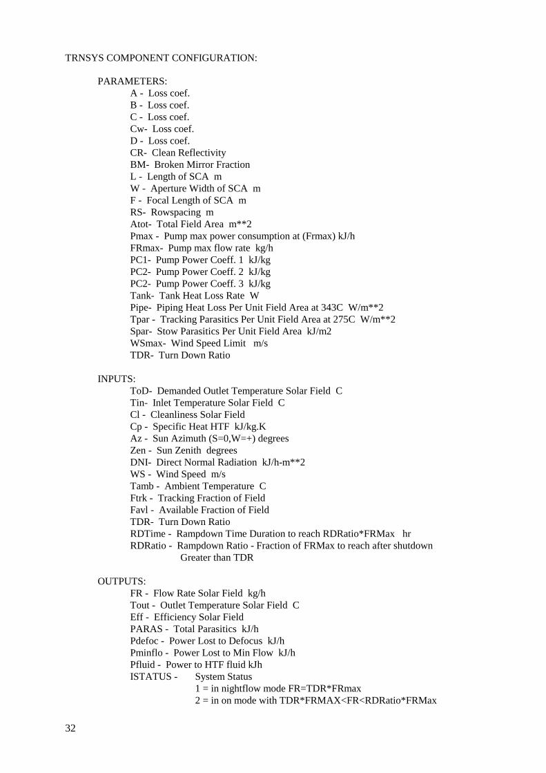
PARAMETERS:A - Loss coef.B - Loss coef.C - Loss coef.Cw- Loss coef.D - Loss coef.CR- Clean ReflectivityBM- Broken Mirror FractionL - Length of SCA mW - Aperture Width of SCA mF - Focal Length of SCA mRS- Rowspacing mAtot- Total Field Area m**2Pmax - Pump max power consumption at (Frmax) kJ/hFRmax- Pump max flow rate kg/hPC1- Pump Power Coeff. 1 kJ/kgPC2- Pump Power Coeff. 2 kJ/kgPC2- Pump Power Coeff. 3 kJ/kgTank- Tank Heat Loss Rate WPipe- Piping Heat Loss Per Unit Field Area at 343C W/m**2Tpar - Tracking Parasitics Per Unit Field Area at 275C W/m**2Spar- Stow Parasitics Per Unit Field Area kJ/m2WSmax- Wind Speed Limit m/sTDR- Turn Down Ratio

INPUTS:ToD- Demanded Outlet Temperature Solar Field CTin- Inlet Temperature Solar Field CCl - Cleanliness Solar FieldCp - Specific Heat HTF kJ/kg.KAz - Sun Azimuth (S=0,W=+) degreesZen - Sun Zenith degreesDNI- Direct Normal Radiation kJ/h-m**2WS - Wind Speed m/sTamb - Ambient Temperature CFtrk - Tracking Fraction of FieldFavl - Available Fraction of FieldTDR- Turn Down RatioRDTime - Rampdown Time Duration to reach RDRatio*FRMax hrRDRatio - Rampdown Ratio - Fraction of FRMax to reach after shutdown

Greater than TDR

OUTPUTS:FR - Flow Rate Solar Field kg/hTout - Outlet Temperature Solar Field CEff - Efficiency Solar FieldPARAS - Total Parasitics kJ/hPdefoc - Power Lost to Defocus kJ/hPminflo - Power Lost to Min Flow kJ/hPfluid - Power to HTF fluid kJhISTATUS - System Status

1 = in nightflow mode FR=TDR*FRmax2 = in on mode with TDR*FRMAX<FR<RDRatio*FRMax

33

3 = in on mode with RDRatio*FRMax<FR<FRMax4 = in shutdown (RDTime and RDRatio applicable)

Old trough (Type 197)

This model is the former parabolic trough type 96 from release 1.0. The difference to type 196 is an

alternative formulation of the absorber efficiency model. Therefore the empirical coefficients A, B, C,

CW, D have different number values.

Parabolic trough (Type 296)

OBJECTIVE: This model is based on the parabolic trough type 197 (old trough). The main advantage

of this model is that for any orientation of the collector the incident angle IA can be calculated.

( )( )( )2180cos1)cos()cos()cos(1)cos( OrAzElTiltTiltElIA −+−⋅⋅−−+−=

The collector shading Sh for the defined orientation is calculated by using the tracking angle phi

( ) ( ) ( )( ) ( ) ( ) ( )( )OrAzcocElTiltTiltEl

OrAzElphi−−−⋅⋅+−

−−⋅=1801cossinsin

180sincostan

( )RS

phiRSWn

n

row

rowSh

cos11 ⋅−⋅

−−=η

TRNSYS COMPONENT CONFIGURATION: (additional parameters with respect to

type 196)

PARAMETERS:

Tilt – tilt of axis (0° = horizontal)OR – orientation in N-S direction (Süd=0, W=+)phimin - min tracking anglephimax - max tracking angleTyp

1 : LS 3 with IAM from SANDIA2 : IST with IAM from SANDIA3 : IST with IAM from DLR

Tower receiver (Type 195)

OBJECTIVE: The receiver model is like the trough model in that it provides as output the flow rate

required to achieve the outlet temperature set point.

34

Since our initial heliostat field model, like SOLERGY, is based upon a simple field efficiency table

interpolation, only the total power to the receiver is calculated. To find the detailed flux distribution

on the receiver, a complex numerical convolution, or ray-trace optical model, must be used. Without

detailed flux information, an empirical receiver heat loss model is more appropriate than one based on

heat transfer relations at the receiver’s surface. In this model, the conductive losses are neglected in

the calculation of the net absorbed power,

radconvincnet QQQQ ���� −−= α

where the subscripts inc, conv, and rad stand for the incident power, the power losses to convection, and

the power losses to radiation. The losses are described by third order polynomials with user-supplied

coefficients:

33

2210 VCVCVCCQconv +++=�

33

2210 incincincrad QRQRQRRQ ���� +++=

where V is the wind velocity. The user can also specify the turn down ratio- below which the power is

discarded. The receiver efficiency,η = QQ

net

inc is also provided as an output.

TRNSYS COMPONENT CONFIGURATION:

PARAMETERS:Efficiency

INPUTS:IP = Incident Power kJ/hrTCI = Fluid inlet temperature CFLCI= Fluid inlet flow rate kg/hrPCO = Fluid outlet pressure BARTS = Temperature set point CCP = Fluid Specific Heat kJ/kg.K

OUTPUTS:FLD = Flow rate demand kg/hrFLCO= Fluid outlet flow rate kg/hrTCO = Fluid outlet temperature CPCI = Fluid inlet pressure BAR

35

Pressurized air receiver (Type 222)

OBJECTIVE: This type can be used for steady state simulation of a pressurised air receiver. The

receiver outlet temperature, pressure and enthalpy are calculated depending on inlet conditions of the

air flow and the radiation input. A simple black body radiation model is included to calculate the

receiver efficiency.

( ) .15.2735.0

,

,,

4

++⋅=

⋅⋅⋅−=

outairinairabs

absrad

absoptrec

tt

PA

T

Tσεηη

Other model equations can be included easily. Receiver body and piping heat losses as well as

receiver cooling losses can be calculated. The pressure loss depending on temperature, pressure and

mass flow can be calculated. Type 222 checks for lower and upper radiation flux limits and has 6

different operation modes when the flux limits are violated:

11 12 13 - low flux: warning only

21 22 23 - low flux: bypass

high flux: warning only bypass stop

TRNSYS COMPONENT CONFIGURATION:

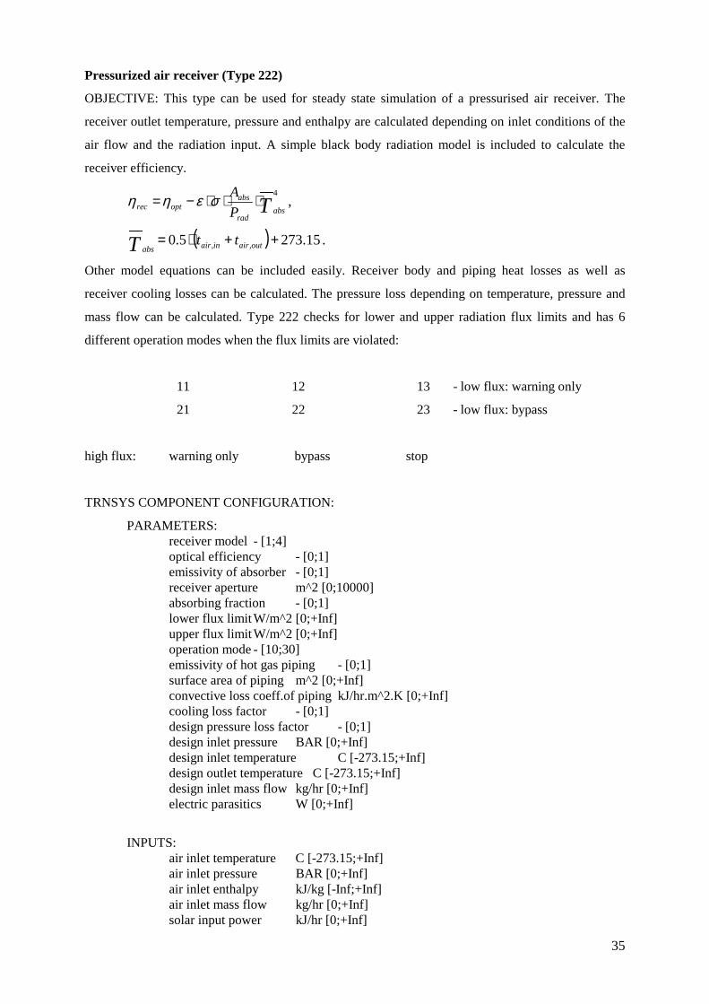
PARAMETERS:receiver model - [1;4]optical efficiency - [0;1]emissivity of absorber - [0;1]receiver aperture m^2 [0;10000]absorbing fraction - [0;1]lower flux limitW/m^2 [0;+Inf]upper flux limitW/m^2 [0;+Inf]operation mode - [10;30]emissivity of hot gas piping - [0;1]surface area of piping m^2 [0;+Inf]convective loss coeff.of piping kJ/hr.m^2.K [0;+Inf]cooling loss factor - [0;1]design pressure loss factor - [0;1]design inlet pressure BAR [0;+Inf]design inlet temperature C [-273.15;+Inf]design outlet temperature C [-273.15;+Inf]design inlet mass flow kg/hr [0;+Inf]electric parasitics W [0;+Inf]

INPUTS:air inlet temperature C [-273.15;+Inf]air inlet pressure BAR [0;+Inf]air inlet enthalpy kJ/kg [-Inf;+Inf]air inlet mass flow kg/hr [0;+Inf]solar input power kJ/hr [0;+Inf]

36

control signal - [0;1]ambient temperature C [-273.15;+Inf]

OUTPUTS:air outlet temperature C [-273.15;+Inf]air outlet pressure BAR [0;+Inf]air outlet enthalpy kJ/kg [-Inf;+Inf]air outlet mass flow kg/hr [0;+Inf]net thermal power kJ/hr [-Inf;+Inf]thermal efficiency - [0;1]pressure loss factor1 - [0;1]parasitic power kJ/hr [0;+Inf]operation status- [0;1]flux overload - [0;+Inf]optimum gas mass flow to reach

design output temperature m_opt kg/hr [-inf;inf]

Heliostat field (Type 194)

OBJECTIVE: The heliostat field model requires a user-supplied field efficiency matrix to evaluate

the field efficiency, ηfield , as a function of the date and time. The power to the receiver is evaluated

by:

�Q A Irec fleld field field= ⋅ ⋅ ⋅ ⋅ρ η Γ

using total mirror surface Afield, reflectivity ρfield, direct normal radiation I and a control parameter Γdescribing the fraction of the field in track. The model also considers electrical parasitics for tracking,

start-up, and shutdown. Shutdown is performed automatically at high wind speeds.

The efficiency matrix gives the heliostat field efficiency for a number of pairs of solar azimuth and

zenith angle. This file is read in and interpolated by the TRNSYS routine data (see manual). The

number of solar elevation and azimuth data points must be specified in the parameters of this type.

The file has the following format

1. line : list of all solar azimuth data points (e.g. for 3 points -120 0 120) (rising order)

2. line : list of all solar zenith angles (eg. for 3 points 0 45 90) (rising order)

following lines with efficiency data for the solar angle data pairs

(-120,0);(-120,45);...;(120,90) with a maximum of 80 characters per line and minimum of one data

point per line. A test printout of the matrix can be found in the list file, when Trnsys is run, which

should be checked. Since the original Trnsys data routine is limited to 5 values for the azimuth angles,

the file data3.for should be linked to the Trnsys code, which uses increased limits (30). The matrix is

linear interpolated using the inputs of the actual solar azimuth and elevation angle.

37

TRNSYS COMPONENT CONFIGURATION:

PARAMETERS:Iufeld = Logical Unit No of Field efficiency input data (File)nel = Number of zenith angle data points in field efficiency filenaz = Number of azimuth angle data points in field efficiency filenhel = Number of Heliostatsfmirror = Mirror Surface per heliostat (m2)rhohel = Reflectivity of heliostatqstart = Elektric work for Startup of one heliostat (KJ)prun = Electric power for tracking one heliostat (kJ/h)vmax = Maximum tolerable wind speed (m/h)

INPUTS:DNI = Direct Norml Insulation (kJ/hm2)vwind = Wind Speed (m/h )gamma = Control Parameter ( 0= Field off, 0.5 = 50% of Field focussing, 1.0 Total field working)theta = Solar zenith angle (is delivered by Standard trnsys type 16 'Solar

radiation Processor')phi = Solar azimuth (is delivered by Standard trnsys type 16 'Solar Radiation

Processor')

OUTPUTS:PTR = Power to receiver (kJ/h)PDEFOC = Power which was defocussed due to control constraints or wind speed (Gamma<1) (kJ/h)PPARASi = Parasitic power for tracking (kJ/h)etafeld = field efficiency

4.5 MODELS OF THE STORAGE SUBLIBRARY

Concrete/Oil thermal storage (Type 230)

OBJECTIVE: This model describes a concrete thermal storage for single phase fluid (HTF oil,

water). It consists of parallel equally spaced tubes in concrete with HTF flowing through in two

possible directions :

flow down (normally charge flow entering hot)

flow up (normally discharge flow entering cold).

The main difference to Standard TRNSYS Type10 Rockbed is the three node temperature model:

fluid temperature - concrete temperature - ambient temperature.

The model includes thermal capacity of concrete mass, thermal capacity of HTF and thermal loss of

concrete to environment. It does not include thermal capacity of (steel) pipe in concrete. Convective

and conductive heat transfer perpendicular to flow direction are considered. Axial conduction are not

included.

The number of nodes in flow direction can be chosen deliberately (10 nodes are normally sufficient).

38

TRNSYS COMPONENT CONFIGURATION:

PARAMETERS:HTF specific heatHFT densitytotal cross sec. area of pipeslength of storageconcrete specific heatconcrete total massreference overall heat transfer coefficientoverall loss coefficientnumber of nodesreference flow rateak0 – ak5 -5 Parameters for scaling of heat transfer coefficient as:

5

5

4

4

3

3

2

210 ��

�

�

��

�

�⋅+

��

�

�

��

�

�⋅+

��

�

�

��

�

�⋅+

��

�

�

��

�

�⋅+⋅+=

refrefrefrefrefref mmak

mmak

mmak

mmak

mmakak

UAUA

�

�

�

�

�

�

�

�

�

�

INPUTS:HTF temperature entering on topHTF flow rate entering on topHTF temperature entering at bottomHTF flow rate entering at bottomambient temperature

OUTPUTS:HTF temperature at bottomHTF flow downHTF temperature on topHTF flow upconcrete mean temperaturetotal energy stored since simulation startconcrete temperature on topconcrete temperature in middle nodeconcrete temperature on bottomheat power to storageheat power to fluidheat storedheat loss

Rockbed thermal storage

(this is standard TRNSYS type 10; please refer to the TRNSYS manual for details)

Variable volume tank

(this is standard TRNSYS type 39; please refer to the TRNSYS manual for details)

39

5 EXAMPLE APPLICATIONS

Some example applications are provided within the example project folder1:

1. A central receiver system (without power cycle) called ‘stec_crs_akt.tpf’

2. A parabolic trough system with steam generator called ‘stec_dcs_akt.tpf’

3. A parabolic trough plus concrete thermal storage system called ‘stec_storage_akt.tpf’

4. A steady state Rankine cycle called ‘stec_cyc_akt.tpf

5. A solar-fossil hybrid Brayton cycle called stec_solargt_akt.tpf

There are no limitations regarding the combination of the solar system with the Rankine cycle or

thermal energy storage components. However, these simple examples have been selected, because

they demonstrate the application of the developed components without being too complex.

1 Example 1, 2 and 4 are from the previous release 1.0 of the STEC distribution and were adapted to TRNSYS 15. Example 3 is from the last release, Example 5 is new with

this release. The following illustrations still feature the pictures from the older Iisibat 2, so some icons will be different in the actual distributed version.

40

5.1 CENTRAL RECEIVER SYSTEM

Figure 4 : Set- up of central receiver system in the IISibat environment

In this example, the IISIbat macro feature is widely used. The first window (figure 4,left side) show

the central receiver set-up as a macro icon ('towerdel') that is linked to two output components: type

25-1 is a standard TRNSYS printer routine that prints the connected information to a data file and

Type65-1 is the standard TRNSYS component which plots the connected quantities online (during the

simulation runs) to the screen (see figure 5).

The 'towerdel'-macro (top-right) consists of another macro module named 'CRS-1' and the STEC

model for the thermal capacity. As explained in section 3.8, the thermal capacity model can be linked

to each component to consider capacity effects. In this case the receiver outlet flow and outlet

temperature is linked to the inlet flow and temperature of the capacity model.

The 'CRS-1' macros itself consists of 4 basic components: the TRNSYS standard data file reader

'Barst9-1', the standard TRNSYS radiation processor 'type16-1', the field efficiency model 'FEffMa-1'

and the Central Receiver model 'CenRec-1'. The links between these components are the direct normal

radiation and wind speed from the data reader to the field efficiency model, the solar zenith and

azimuth angle from the radiation processor to the field efficiency model and the power from the field

efficiency model to the central receiver. The radiation processor additionally requires radiation data to

evaluate azimuth and elevation angle. This processor is also able to calculate Direct Normal

Insolation data from global and diffuse radiation data .

Part of the output of the calculation for one day is presented in figure 5. It shows the field efficiency,

the direct normal insolation (in kJ/m²h), the receiver flow rate to meet the setpoint temperature and

the outlet temperature of the thermal capacity model, which is used in this case to describe the start-

up and shutdown characteristic of the receiver.

41

Figure 5: Output of the Online Plot component Type 65 during a 1 day simulation of the central receiver

system

The outlet temperature of the receiver is still high when the DNI dropped to zero, because the flow

rate is zero, so that the temperature reflects the thermal capacity of the receiver mass.

DNI

Eta_field

Flow rate

Outlet temp.

42

5.2 PARABOLIC TROUGH SYSTEM WITH STEAM GENERATOR

The assembly of the parabolic trough project is shown in figure 6. It consists three icons (figure 6 top)

representing the macro model for the parabolic trough field (DCS-1), the thermal capacity model and

the macro icon of the steam generator (dynsteam-1).

Figure 6 : Set-up of the trough system with steam generator in the IISibat environment

The DCS-1 macro is similar to the CRS-1 macro in the example discussed above. It consists of the

standard TRNSYS data reader component (Barst9-1), the standard TRNSYS radiation processor and

the STEC Parabolic trough model. The steam generator macro consists of the STEC model of the

economiser heat exchanger (ECO-SH-1) , evaporator heat exchanger (Evapor-1), the superheater heat

exchanger (ECO-SH-2) and a thermal capacity model (inerti-1).

The links between the components consider two fluid circuits: The heat transfer fluid (HTF) , which

is circulated through the trough and the steam generator, and the water steam circuit which has an

open end at the feed water of the economiser inlet and an open end at the steam conversion utility

function output in this example. The quantities which need to be linked depend on the circuit in the

system. In the HTF fluid circuit, temperature and mass flow rate are connected from the output of the

component (in flow direction) to the input of the next component. The pressure is not considered as

information here. In the water/steam circuit, additionally the quality and pressure are used. In the

turbine models, enthalpy is used instead of temperature and quality. These quantities are also

connected in the flow direction. In contrast to that, the pressure information is connected opposite the

flow direction: i.e. the pressure information travels from the flow inlet side of one component to the

flow outlet side of its upstream component. This approach significantly improves the numerical

convergence of the model.

The HTF mass flow rate is determined in this example by the parabolic trough model, in order to meet

the temperature set-point condition. The steam flow rate results from the HTF flow rate, HTF outlet

43

temperature and the heat exchanger characteristics. The evaporator model demands for a the

according feed water flow rate. This demand signal is linked directly to the economiser inlet flow

input in this example. It could also be linked to a pump model which would have the additional

impact that the power consumption for the pump and the limitation to a maximum flow rate would be

considered also.

The influence of the thermal capacity models of the solar field and of the steam generator can be seen

from the calculations results for a clear day operation as presented in figure 7. The HTF temperature

is rising later than the direct normal insolation (DNI) due to the capacity of the capacity components.

The evaporator model starts to demand for steam flow after the HTF has reached the boiling

temperature of the water at the respective system pressure. Therefore, a time delay for the collector

outlet temperature relative to the solar insolation as well as a delay of the steam production relative to

the collector operation can be simulated achieved by the models.

6 7 8 9 10 11 12 13 14 15 16 17 18

0

200

400

600

800

1000 D N I

DN

I [W

/m²]

T im e o f D a y [h ]

050

100150200250300350

S ta rt B o ilin g

T H T F

T stea mTem

pera

ture

[°C

]

01 0 02 0 03 0 04 0 05 0 06 0 0

Flow

Rat

e [t

/h]

H T F -F lo w S te am F lo w

Figure 7: Results from a 1 day calculation of the trough system with steam generator

44

5.3 TROUGH AND STORAGE COMBINATION

Figure 8: Setup of trough/storage combination

Key components of this example are the well known trough model (former type 96, now type 197)

and the new model for concrete thermal storage (type 230). A simple charge/discharge controller

(type 231) is added, which decides if the demand can be met directly solar or by the storage. Concrete

thermal storages exhibit a characteristic temperature profile. They are charged by a hot fluid (here:

hot oil from solar field) flowing through parallel pipes in a certain flow direction, heating the

surrounding concrete material. While charging, the hot temperature front moves slowly with the flow

direction along the storage. When the fluid leaving the storage exceeds a certain temperature limit

(here: 320°C) the storage is said to be full and the charging process is stopped. Otherwise the thermal

losses in the solar field would rise extremely. Accordingly, the storage is discharged by a cold fluid

flowing in the opposite direction and cooling the concrete. When the cold temperature front reaches

the end and the hot fluid falls short of a certain lower temperature limit the storage is said to be empty

and the discharging process is stopped. Otherwise the efficiency of the demanding unit (e.g. steam

cycle) would drop significantly.

45

270

300

330

360

390

144 146 148 150 152 154 156 158 160 162 164 166 168Time [hr]

Tem

per

atu

re [

°C]

T_solar [øC]

T_HTF_top [øC]

T_HTF_bott [øC]

T_c_top [øC]

T_c_bottom [øC]

T_use [øC]

0.00E+00

2.00E+05

4.00E+05

6.00E+05

8.00E+05

1.00E+06

144 146 148 150 152 154 156 158 160 162 164 166 168

Time [hr]

Flo

w R

ate

[kg

/hr]

M_solar [kg/hr]

M_charge [kg/hr]

M_discharge [kg/hr]

M_demand [kg/hr]

M_use [kg/hr]

Figure 9: Results from a 1 day simulation of the trough/storage combined system

Figure 9 shows the simulation results from day 6 of the included example. There is a time shift

between the solar field operation (from about 8:00 to 17:00) and the heat demand (from 12:00 to

22:00). Hence the storage is charged in the morning hours (charge flow: pink line) by the hot HTF

from the solar field (390°C dark blue line). The oil and concrete temperatures in the storage increase.

The charge flow decreases as the demand rises and stops at 12:00. When the solar flow exceeds the

demand (14:00-16:00), the storage cannot be charged as the oil exit temperature has reached the limit

of 320°C. When the direct solar heat supply ends (16:30) the storage is discharged (discharge flow:

yellow line) until the oil temperature falls below 360°C (at about 21:00). The demand until 22:00

cannot be met in this case.

46

5.4 SIMPLE RANKINE CYCLE

The set-up of the Rankine cycle is shown in Figure 10 and Figure 11. It consists of a boiler section

which is similar to the example given above. Down stream of the boiler a steam turbine with two

extraction lines is presented by three turbine stage modules (nstage-1, nstage-2, nstage-3) and two

extraction splitters (ex1, ex2). A standard TRNSYS calculator utility component (Totpower) is used

to add up the mechanical power production of all three stages. The final turbine stage is connected to

the condenser module (Conden-1). The two extraction splitters are linked to the deaerator module

(deart-1) and the feedwater heater macro (feedwt-2). This macro consist (as shown in figure 8 lower

left side) of a condensing preheater (preheat-1) and a subcooler module (subcool-1). Additionally a

condenser pump (CondPu) and a feedwater pump (FWPu) are part of the system.

Figure 10 : Set-up of the Rankine cycle in the IISibat environment

The relevant links are discussed in the following:

47

The evaporator demand flow signal is linked to the control input of the feedwater pump which sets the

flow rate of the whole system. The condenser pump model uses the input flow rate as flow demand

signal.

Flow rate and enthalpy are connected from turbine stage outlet to splitter and further from the splitter

outlet to the turbine stage inlet. The pressure is connected in the opposite direction from condenser to

turbine stage outlet to splitter inlet and so on. Pressure and enthalpy are connected from the second

splitter outlet to the preheater/dearator inlet is whereas the steam flow rate (demand) is connected in

the opposite direction.

The feedwater flow rate and temperature from the condenser outlet is linked first to the pump, then to

the deaerator, then to the feedwater pump, then to the preheater and then to the economiser inlet.

The temperature, quality and flow rate of the condensed extraction steam in the condensing preheater

is linked to the inlet of the subcooler and further to the condensate inlet of the dearator.

It is obvious from this example that the set-up of such as system may become rather complex.

Therefore it is recommendable to generate macro model for all kinds of subsystems which may be

used again later. Thereby, the configuration and all the relevant links of the subsystem is saved and

the set-up of new systems can be performed with less effort and a lower probability of making errors.

Inexperienced users should develop a new system model in small steps combining components in to

subsystems that can be stored as macros. These macros should be individually tested by linking

standard TRNSYS input functions (type14) to vary the essential input quantities. The essential output

can be connected to the online plotter. After each subsystem macro is checked, the whole system can

be set-up by connecting them together.

In order to verify the steady state performance of the components for the Rankine cycle, the

commercial Computer Code KPRO [7] was used to evaluate the thermodynamic design performance

data of a fictive Rankine cycle as presented in. The results of the TRNSYS code and its deviation

from KPRO are presented for temperature, pressure, and mass flow rate at all relevant locations of the

plant. The calculation was based on equal overall heat transfer factors for all heat exchanger units,

equal reference pressure losses, and the same inner turbine efficiencies, turbine reference mass flow

rates and reference pressures. shows that the conformity of both codes is excellent. For the electrical

power output, there was a 0.6 % difference between the values computed by each code. Slight

differences may result from different formulations of the property functions. The function used in

defined TRNSYS is less precise but much faster than the one used in KPRO. An annual performance

calculation ran in less than 5 minutes on a fast PC (0.03 sec/time step) whereas it took more than 10

48

sec on KPRO for a single run. KPRO itself is neither able to perform calculations over time (e.g.

annual runs), nor consider capacity effects and can not be expanded by user components.

Cooling Tower

Evaporator

Economizer

Superheater

Condenser

CondensatePumpSubcooler

Deaerator

FeedwaterPump

Turbine Generator

Steam Condenser

T=573.8M=36

T=491.6 + 0

T=316.7 +0

T=251.4 -0.5

T=499.9 +0.1P=100.1 -0.1

H=3019+0P=20.02-0.02M=0.5 +0

T=311.7 +0.0P=101.1 -0.1

T=306.6 +0.1P=102.1 -0.1

T=207.8 -0.4P=103.1 -0.1M=5.0 +0.

T=212.4 +0 T=157.4 +1.7

T=151.8 +0

T=212.4 +0

H=2781 +1P=5.0 +0M=0.84 -0.01

T=35.0 +0M=3.66 +0.01

H=2249 +1P=0.56 +0M=3.66 +0

T=20M=184 +0

T=30

Pel=4761-30

Results of KPRO and TRNSYS Calculations

T in °CP in barM in kg/sH in kJ/kgPel in kW

Figure 11: Results from TRNSYS for a fictive Rankine cycle. The sum of both values are KPRO results

(italic data are inputs).

5.5 SOLAR-FOSSIL HYBRID BRAYTON CYCLE

This example is new with release 2.2 of the STEC library and shows the use of the DLR models from

the Brayton sublibrary together with the CRS models. It uses the new pressurised air receiver model

(type 222). Figure 12 shows the Iisibat set-up of this project. It models a simple Brayton-cycle with a

tower receiver acting as a of the pressurised air before it enters the combustion chamber, where the air

is heated further to reach the desired turbine inlet temperature . Figure 13 shows an example plot of

the system simulation. One can see the receiver heating the air from around 400°C up to almost 800°C

depending on the solar input, while the turbine inlet temperature remains constant at 1100°C. Hence,

the maximum solar contribution in this fuel saver concept is limited to about 60%. Clearly can be seen

the reduced electric output when the solar input in increased. This is due to less total mass flow in the

turbine because of the reduced fuel input.

49

Figure 12: Screenshot of Iisibat model-setup for solar hybrid gas turbine (Brayton) cycle.

Figure 13: Screenshot example plot for solar hybrid gas turbine (Brayton) cycle.

DNI

turbine inlet temp.

receiver outlet temp.

power to receiver

electric output power

50

6 REFERENCES

[1] Stoddard, M.C., Faas, S.E., Chiang, C. J. and Dirks, A.J., SOLERGY - A Computer Code for Calculating the

Annual Energy from Central Receiver Power Plants, SAND86-8060 Sandia National Laboratories, Livermore,

CA, 1987.

[2] TRNSYS, A Transient Simulation Program, Vers. 14.2, Solar Energy Laboratory, University of Wisconsin,

Madison, 1995.

[3] Lippke, F, Simulation of the Part-Load Behavior of a 30 MWe SEGS Plant, SAND95-1293, Sandia National

Laboratories, Albuquerque, NM, 1995.

[4] Kays, W. M. and London, A.L. , Compact Heat Exchangers, McGraw-Hill, 1958.

[5] Popel, O.S., Fried, S.E. and Sphilrain, E.E., Solar Thermal Power Plants Simulation Using TRNSYS Software,

9th International Symposium Solar Thermal Concentrating Technologies, June, 22-26, 1998, Odeillo, France.

[6] Shpilrain, E.E., Popel, O. S., Frid, S. E., Advanced Solarized Cycles, SolarPACES Technical Report, No III 3-

98, 1998.

[7] KPRO, Programm zur Berechnung von Kreisprozessen (Simulation Code for the Evaluation of Power Cycles),

Vers. 4.1. Fichtner, Stuttgart, 1997.

[8] Dudley V.E. et al.: SEGS LS-2 Solar Collector. Test Results. Sandia National Laboratories 1994. SAND94-1884

51

Appendix

A1. System Requirements to use TRNSYS and the STEC Library

The new release 2.2 of the STEC library was designed for the latest updates of TRNSYS 15 and the

user Interface IISibat Version 3 (September 2002: TRNSYS version 15.2.07, IIsibat version 3.0.021).

Ask your TRNSYS provider for the appropriate version. The TRNSYS code itself, which is the

computational kernel, is written in Fortran. In principle, it can be compiled on any computer system

with an ANSI Fortran compiler. However, the online plotter is only supported in Windows95 and

Windows NT. Without this feature, only ASCII output files can be generated by TRNSYS.

The graphical user interface IISIbat runs on Windows95 / Windows NT (preferred) and requires a fast

Pentium processor and at least 32Mbyte of Ram to allow an acceptable editing performance. The

IIsibat user interface generates an ASCII input file on the basis of the user configuration and can start

the TRNSYS calculation process automatically.

The performance of a fast Pentium computer is sufficient in most cases to run annual calculation in a

few minutes time.

In order to set-up new models or modify the source code of existing models, a 32 bit Fortran compiler

is required which has to rebuild the source code as a 32 bit Windows dynamic link library (dll). The

trnlib.dll distributed with this Stec release was built with the Compaq Visual Fortran Version 6.1.0

Compiler. A lot more information about this topic can be found on the TRNSYS web page

(http://sel.me.wisc.edu/TRNSYS/ � Fortran Information...)

52

A2. Installation of the STEC Library

To install the library follow the instructions in the README file that is included in the stec_2.2.zip

file:

******************************************************************************** R E A D M E notes for S T E C R E L E A S E 2.2 ** ** Date: 20.09.2002 ** Last modification: 20.09.2002 ** Author: P. Schwarzboezl, DLR ** ********************************************************************************

*** Information ***

> The STEC_2.2.zip archive contains all relevant files to run theTRNSYS STEC library and associated example projects.

> TRNSYS version 15.2.07 and the GUI Iisibat version 3.0.0.21 were usedto create the model files and example projects.

> Compaq Visual Fortran Professional Edition 6.1.0 was used to createthe STEC_2.2_trnlib.dll.

> WINZP 7.0 was used to create the zip-archive.

*** Installation Notice for STEC Release 2.2 ***

====> Extract the content of the archive to the location of yourTRNSYS15 programme (e.g. 'c:\trnsys15\'). The subfolders andfiles are extracted to the corresponding folders.

> The components' proforma files (*.tmf, *.bmp) are extracted to'c:\trnsys15\IIsibat3\Data\STEC Library Release\..'

> The source code files (xxx.for) are extracted to'c:\trnsys15\Types\stectypes\..'

> The stec example projects (*.tpf) are extracted to'c:\trnsys15\IIsibat3\Data\Samples\STEC_release_examples\..'

> Weather and other data files are extracted to'c:\trnsys15\Weather\..'

> The trnlib.dll is extracted as 'stec2.2_trnlib.dll' to'c:\trnsys15\DLLs\..' to avoid overwriting of the existing dll!It has to be renamed before use and copied to 'c:\trnsys15\..' !

NOTICE:If you prefer to move the stec related files into your trnsysfolder-structure by hand, simply let the archive be extracted to atemporary folder (e.g. 'c:\Temp\..') and copy the files afterwardsto the right destiny.

>>>>>> If you have problems or suggestions you can contact me at:

peter.schwarzboezl@dlr.de

********************************************************************************

53

That's it! Now you can start the examples from the 'stec_Examples' folder and try to run them or

create new projects using the models form the STE, Rankine and Brayton sublibs. To create your

own dll to use the STEC types you have to include the files of the stectypes-folder into your compiler

project.

Please note that with signing the user agreement and receiving the STEC library models you

committed yourself to provide the source code and sufficient documentation of own developments to

the other users. Therefore, please send your own model developments, example projects and

documentation to peter.schwarzboezl@dlr.de to have them included into the next STEC library

release.