THE VOLATILITY OF LIQUIDITY AND EXPECTED STOCK

RETURNS

A Dissertation

by

FERHAT AKBAS

Submitted to the Office of Graduate Studies of

Texas A&M University

in partial fulfillment of the requirements for the degree of

DOCTOR OF PHILOSOPHY

August 2011

Major Subject: Finance

The Volatility of Liquidity and Expected Stock Returns

Copyright 2011 Ferhat Akbas

THE VOLATILITY OF LIQUIDITY AND EXPECTED STOCK

RETURNS

A Dissertation

by

FERHAT AKBAS

Submitted to the Office of Graduate Studies of

Texas A&M University

in partial fulfillment of the requirements for the degree of

DOCTOR OF PHILOSOPHY

Approved by:

Co-Chairs of Committee, Sorin M. Sorescu

Ekkehart Boehmer

Committee Members, Michael F. Gallmeyer

Asqhar Zardkoohi

Head of Department, Sorin M. Sorescu

August 2011

Major Subject: Finance

iii

ABSTRACT

The Volatility of Liquidity and Expected Stock Returns. (August 2011)

Ferhat Akbas, B.S., Bilkent University;

M.S., Texas A&M University

Co-Chairs of Advisory Committee: Dr. Sorin M. Sorescu

Dr. Ekkehart Boehmer

The pricing of total liquidity risk is studied in the cross-section of stock returns.

This study suggests that there is a positive relation between total volatility of liquidity

and expected returns. Our measure of liquidity is Amihud measure and its volatility is

measured using daily data. Furthermore, we document that total volatility of liquidity is

priced in the presence of systematic liquidity risk: the covariance of stock returns with

aggregate liquidity, the covariance of stock liquidity with aggregate liquidity, and the

covariance of stock liquidity with the market return. The separate pricing of total

volatility of liquidity indicates that idiosyncratic liquidity risk is important in the cross

section of returns.

This result is puzzling in light of Acharya and Pedersen (2005) who developed a

model in which only systematic liquidity risk affects returns. The positive correlation

between the volatility of liquidity and expected returns suggests that risk averse

investors require a risk premium for holding stocks that have high variation in liquidity.

Higher variation in liquidity implies that a stock may become illiquid with higher

iv

probability at a time when it is traded. This is important for investors who face an

immediate liquidity need and are not able to wait for periods of high liquidity to sell.

v

ACKNOWLEDGEMENTS

I would like to thank my advisors, Dr. Sorin Sorescu, Dr Ekkehart Boehmer, and

Dr. Michael Gallmeyer, for their support and guidance throughout the course of this

research. I also want to thank my colleagues, Dr. Ralitsa Petkova and William J.

Armstrong, for their endless patience and continuous support during frustrating times of

job searching and frustrating moments of writing my dissertation. As a funny

coincidence of life, missing a plane in Atlanta helped me to write my dissertation.

Special thanks go to my colleagues, Egemen Genc, who caused me to miss the plane and

who supported me, even over the phone, numerous times during research and to Emre

Kocatulum, who convinced me to change my research area to Finance. Also I would like

to thank my friends, Tayfun Tuysuzoglu, Bekir Engin Eser, Ahmet Caliskan, Bilal

Erturk, Osman Ozbulut, Sami Keskek, Renat Shaykhutdinov, Selcuk Celil, Fatih

Ayyildiz, Ibrahim Ergen, and Selahattin Aydin.

I received many useful comments from workshop participants in the Texas

A&M University Department of Finance. I also wish to extend my gratitude to the Mays

Business School for generous financial support and the Texas A&M University

Department of Economics.

Finally, special thanks to my mother, Esvet Akbas, my father, Mehmet Akbas,

and, my brother, Murat Akbas, for their love, patience, prayers, and support. During the

last year of graduate studies, my fiancée was my source of energy and courage in writing

this dissertation.

vi

TABLE OF CONTENTS

Page

ABSTRACT .............................................................................................................. iii

ACKNOWLEDGEMENTS ...................................................................................... v

TABLE OF CONTENTS .......................................................................................... vi

LIST OF TABLES .................................................................................................... viii

1. INTRODUCTION ............................................................................................... 1

2. EMPIRICAL METHODS ................................................................................... 8

2.1 The Main Measure of Liquidity ........................................................... 8

2.2 Constructing the Volatility of Liquidity ............................................... 9

2.3 Data and Descriptive Statistics ............................................................. 10

3. EMPIRICAL RESULTS ..................................................................................... 15

3.1 Portfolio Approach ............................................................................... 15

3.2 Regression Approach ........................................................................... 18

3.3 Regressions Approach within Size and Illiquidity Groups .................. 22

4. ROBUSTNESS ................................................................................................... 25

4.1 Risk-Adjusted Returns ......................................................................... 25

4.2 Sub-Sample Analysis ........................................................................... 29

4.3 Comparing Daily and Monthly Measures of the Volatility of

Liquidity, Based on Amihud, Turnover, and Dollar Volume………... 32

4.4 Alternative Measurement Periods for the Volatility of Liquidity ........ 39

4.5 Expected Volatility of Liquidity .......................................................... 41

4.6 Additional Robustness Checks ............................................................. 43

5. THE IDIOSYNCRATIC COMPONENT OF VOLATILITY OF LIQUIDITY 45

6. CONCLUSION ................................................................................................... 49

REFERENCES .......................................................................................................... 50

vii

Page

VITA ......................................................................................................................... 55

viii

LIST OF TABLES

TABLE Page

1 Summary Statistics ..................................................................................... 13

2 Average Portfolio Returns .......................................................................... 17

3 Fama-MacBeth Regression Estimates Using Individual Security Data ..... 20

4 Fama-MacBeth Regression Estimates by Size and Illiquidity Groups ...... 23

5 Fama-MacBeth Regression Estimates: Using Risk-Adjusted Returns as

the Dependent Variables ............................................................................ 27

6 Fama-MacBeth Regression Estimates: Sub-Period Analysis ..................... 30

7 Fama-MacBeth Regression Estimates: Comparing Daily and Monthly

Measures of the Volatility of Liquidity Based on Amihud, Turnover,

and Dollar Volume ..................................................................................... 35

8 Fama-MacBeth Regression Estimates: The Role of Short Sale

Restrictions ................................................................................................. 38

9 Fama-MacBeth Regression Estimates: Using Different Measurement

Periods for the Volatility of Liquidity ........................................................ 40

10 Fama-MacBeth Regression Estimates: Using the Predicted Value of the

Volatility of Liquidity ................................................................................ 42

11 Fama-MacBeth Regression Estimates: Using Idiosyncratic Volatility of

Liquidity ..................................................................................................... 47

1

1

1. INTRODUCTION

In this dissertation we document a positive and significant relation between a

stock’s expected return and its volatility of liquidity. The volatility of liquidity is a stock-

specific characteristic that measures the uncertainty associated with the level of liquidity

of the stock at the time of trade. The positive correlation between the volatility of

liquidity and expected returns suggests that risk averse investors require a risk premium

for holding stocks with high variation in liquidity.

Numerous studies have shown that the mean level of liquidity is positively priced

in the cross-section of expected returns.1 The motivation behind examining the second

moment of liquidity is that investors who need to trade at random points in time might

care about not only the mean but also the volatility of the liquidity distribution. This is

the case since liquidity varies over time and higher variation in liquidity implies that a

stock may be very illiquid at a time when it is traded. If a stock’s liquidity fluctuates

within a wider range around its mean compared to otherwise similar stocks, an investor

holding the stock may be exposed to a relatively higher probability of low liquidity at the

time he needs to sell the stock. The volatility of liquidity captures this risk. Therefore,

all else equal, a risk-averse investor may be willing to pay a higher price for a stock that

has a lower risk of becoming less liquid at the time of trading, i.e., a stock whose

This dissertation follows the style of Journal of Finance.

1 See, among others, Amihud and Mendelson (1986, 1989), Brennan and Subrahmanyam (1996),

Eleswarapu (1997), Brennan, Chordia and Subrahmanyam (1998), Chalmers and Kadlec (1998), Chordia,

Roll and Subrahmanyam (2001), Amihud (2002), Hasbrouck (2009), Chordia, Huh, and Subrahmanyam

(2009).

2

2

liquidity is less volatile.2

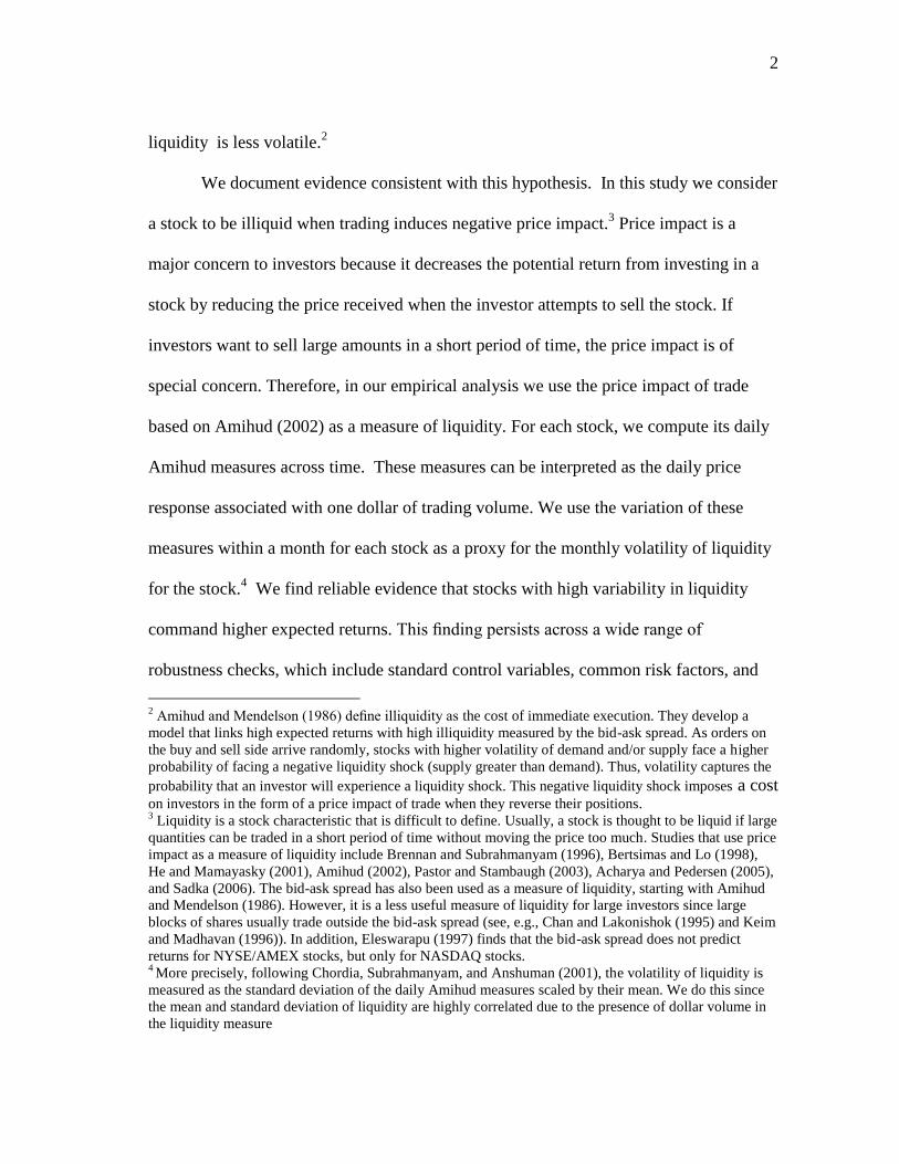
We document evidence consistent with this hypothesis. In this study we consider

a stock to be illiquid when trading induces negative price impact.3 Price impact is a

major concern to investors because it decreases the potential return from investing in a

stock by reducing the price received when the investor attempts to sell the stock. If

investors want to sell large amounts in a short period of time, the price impact is of

special concern. Therefore, in our empirical analysis we use the price impact of trade

based on Amihud (2002) as a measure of liquidity. For each stock, we compute its daily

Amihud measures across time. These measures can be interpreted as the daily price

response associated with one dollar of trading volume. We use the variation of these

measures within a month for each stock as a proxy for the monthly volatility of liquidity

for the stock.4 We find reliable evidence that stocks with high variability in liquidity

command higher expected returns. This finding persists across a wide range of

robustness checks, which include standard control variables, common risk factors, and

2 Amihud and Mendelson (1986) define illiquidity as the cost of immediate execution. They develop a

model that links high expected returns with high illiquidity measured by the bid-ask spread. As orders on

the buy and sell side arrive randomly, stocks with higher volatility of demand and/or supply face a higher

probability of facing a negative liquidity shock (supply greater than demand). Thus, volatility captures the

probability that an investor will experience a liquidity shock. This negative liquidity shock imposes a cost on investors in the form of a price impact of trade when they reverse their positions. 3 Liquidity is a stock characteristic that is difficult to define. Usually, a stock is thought to be liquid if large

quantities can be traded in a short period of time without moving the price too much. Studies that use price

impact as a measure of liquidity include Brennan and Subrahmanyam (1996), Bertsimas and Lo (1998),

He and Mamayasky (2001), Amihud (2002), Pastor and Stambaugh (2003), Acharya and Pedersen (2005),

and Sadka (2006). The bid-ask spread has also been used as a measure of liquidity, starting with Amihud

and Mendelson (1986). However, it is a less useful measure of liquidity for large investors since large

blocks of shares usually trade outside the bid-ask spread (see, e.g., Chan and Lakonishok (1995) and Keim

and Madhavan (1996)). In addition, Eleswarapu (1997) finds that the bid-ask spread does not predict

returns for NYSE/AMEX stocks, but only for NASDAQ stocks. 4 More precisely, following Chordia, Subrahmanyam, and Anshuman (2001), the volatility of liquidity is

measured as the standard deviation of the daily Amihud measures scaled by their mean. We do this since

the mean and standard deviation of liquidity are highly correlated due to the presence of dollar volume in

the liquidity measure

3

3

different sub-periods. Our estimate of the volatility of liquidity is not sensitive to the

measurement horizon and is significant for measurement windows of up to 12 months.

Furthermore, we show that total volatility of liquidity is priced in the presence of

systematic liquidity risk: the covariance of stock returns with aggregate liquidity, the

covariance of stock liquidity with aggregate liquidity, and the covariance of stock

liquidity with the market return. Since total liquidity volatility comes from systematic

and idiosyncratic sources, the pricing of total volatility of liquidity in the presence of

systematic liquidity betas indicates that idiosyncratic liquidity risk is important in the

cross-section of returns. This result has not been shown before. The pricing of

idiosyncratic liquidity risk that we document creates a puzzle in light of Acharya and

Pedersen (2005) who develop a model in which only systematic liquidity risk affects

returns. In particular, total volatility of liquidity affects returns over and above the

three liquidity risk effects documented in Acharya and Pedersen (2005): the

covariance of stock returns with aggregate liquidity, the covariance of stock liquidity

with aggregate liquidity, and the covariance of stock liquidity with the market return.5

Using daily data is key to capturing the dimension of liquidity related to short-

term variability in trading costs. If an investor faces an immediate liquidity need due to

exogenous cash needs, margin calls, dealer inventory rebalancing, forced liquidations,

or standard portfolio rebalancing, he needs to unwind his positions in a short period of

time. In case of such a liquidity need the investor may not be able to wait for periods of

high liquidity to sell the stock, and thus the level of liquidity on the day the investor

closes his position is important. This effect will be reinforced if investors are subject to

5 Other papers that explicitly study the pricing of systematic liquidity risk include Pastor and Stambaugh

(2003) and Sadka (2006), among others

4

4

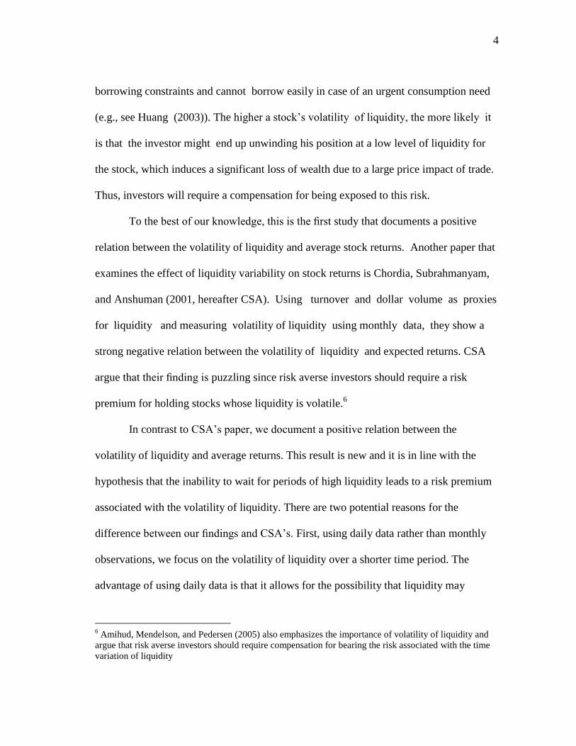
borrowing constraints and cannot borrow easily in case of an urgent consumption need

(e.g., see Huang (2003)). The higher a stock’s volatility of liquidity, the more likely it

is that the investor might end up unwinding his position at a low level of liquidity for

the stock, which induces a significant loss of wealth due to a large price impact of trade.

Thus, investors will require a compensation for being exposed to this risk.

To the best of our knowledge, this is the first study that documents a positive

relation between the volatility of liquidity and average stock returns. Another paper that

examines the effect of liquidity variability on stock returns is Chordia, Subrahmanyam,

and Anshuman (2001, hereafter CSA). Using turnover and dollar volume as proxies

for liquidity and measuring volatility of liquidity using monthly data, they show a

strong negative relation between the volatility of liquidity and expected returns. CSA

argue that their finding is puzzling since risk averse investors should require a risk

premium for holding stocks whose liquidity is volatile.6

In contrast to CSA’s paper, we document a positive relation between the

volatility of liquidity and average returns. This result is new and it is in line with the

hypothesis that the inability to wait for periods of high liquidity leads to a risk premium

associated with the volatility of liquidity. There are two potential reasons for the

difference between our findings and CSA’s. First, using daily data rather than monthly

observations, we focus on the volatility of liquidity over a shorter time period. The

advantage of using daily data is that it allows for the possibility that liquidity may

6 Amihud, Mendelson, and Pedersen (2005) also emphasizes the importance of volatility of liquidity and

argue that risk averse investors should require compensation for bearing the risk associated with the time

variation of liquidity

5

5

change within a month. In contrast, calculating volatility using monthly measures of

liquidity, as CSA do, implicitly assumes that liquidity is constant within a month.

Therefore, daily data enables us to capture the possibility that a negative liquidity shock

and an immediate liquidity need could occur simultaneously over a few days.7

Second, our measure of liquidity differs from the one used by CSA. We use the

price impact of trade based on Amihud (2002), while CSA use trading volume.

Avramov, Chordia, and Goyal (2006) note that trading volume and Amihud’s measure

of liquidity are only moderately correlated and may capture different aspects of

liquidity. While liquidity has many dimensions, we seek to measure the price impact of

trade since it is most relevant for our study. If investors seek to uncover their positions in

a stock in a short time, we need a measure of liquidity which can capture the possibility

of the price moving significantly in the direction of trade. Therefore, we use the price

impact of trade as our primary liquidity measure. A key benefit of the Amihud (2002)

measure is that it can be estimated over a long sample period with a high frequency. In

addition, it gives us the opportunity to measure the volatility of liquidity over a month or

a quarter using daily data.

In a robustness analysis we use both our measure of volatility of liquidity and

the one proposed by CSA. Namely, the volatility of daily Amihud ratios and the

volatility of trading activity over the last 36 months are used in the same regression.

Both measures remain significant with a positive sign and a negative sign, respectively.

7 We assume that impatient investors take liquidity as given at the time they face a liquidity need. That is,

they are unable to wait for periods of high liquidity to reverse their trading positions. If liquidity providers

are able to time their trades to align with periods of high liquidity, competition would eliminate their

ability to earn a risk premium.

6

6

Therefore, our finding that the volatility of liquidity is positively related to returns

should be viewed as complementary rather than contradictory to the results documented

by CSA. CSA offer a possible interpretation of their results using the investor

recognition hypothesis of Merton (1987). Namely, the volatility of trading activity for a

certain stock might proxy for the heterogeneity of the clientele holding the stock. High

volatility could indicate a shift towards a more heterogeneous group of people who want

to hold the stock, therefore lowering the required expected return.8

Pereira and Zhang (2011) develop a rational model that generates results

consistent with CSA’s surprising finding. In their model, investors with certain

investment horizons time the market by waiting for periods of high liquidity to sell their

stocks. The higher a stock’s volatility of liquidity, the more likely it is that there will

be a point at which liquidity is significantly higher resulting in lower costs of

illiquidity for a patient investor. Therefore, Pereira and Zhang (2011) emphasize

investors’ preference for volatility of liquidity due to upside movements in liquidity. In

contrast to Pereira and Zhang (2011), we argue that investors dislike the volatility of

liquidity due to the potential of large downside movements in liquidity. Consistent with

this hypothesis, we also find that the volatility of liquidity effect on expected returns is

stronger in bad economic times when downside movements in liquidity are more likely

and borrowing constraints are higher.

In summary, this dissertation contributes to the literature by documenting that

the positive effect on returns of the volatility of liquidity is different from previously

8 Barinov (2010) argues that controlling for exposure to aggregate market variance explains CSA’s results

7

7

documented effects such as the mean level of liquidity and systematic liquidity risk.

We conjecture that the volatility of liquidity matters most for investors who may face an

immediate liquidity need over a relatively short horizon and are unable to adapt their

trading to the state of liquidity of their stocks.9

For example, in August of 1998 Long

Term Capital Management had to unwind their positions under highly adverse

conditions. A large part of their losses was due to the price impact of trade.10

Volatility

of liquidity is also important for investors that might not be professional traders. For

example, a household may have to liquidate its illiquid assets due to consumptions

needs. Similarly, a firm may have to liquidate certain assets to undertake a surprise

investment opportunity.

The rest of the dissertation is organized as follows. In Section 2 we discuss the

construction of our liquidity measure and the data sample. Section 3 documents the

main results. Robustness tests are presented in Section 4. Section 5 examines the

idiosyncratic component of the volatility of liquidity, and Section 6 concludes.

9 Pereira and Zhang (2010) argue that the possibility of an emergency liquidation of a stock with volatile

liquidity, combined with an uncertain investment horizon, will command an extra liquidity premium due

to the high price impact of trade. This is also in line with the theoretical arguments of Koren and Szeidl

(2002) and Huang (2003) 10

See Lowenstein (2000) for a more detailed story

8

8

2. EMPIRICAL METHODS

2.1 The Main Measure of Liquidity

If an investor faces an immediate need to sell a stock, he may not be able to adapt

his trading to the liquidity state of the stock. Therefore, if he needs to unwind his

position in the stock in a short time he might sell at a very unfavorable price due to the

high price impact of trade. The price impact of trade is the liquidity measure that we are

interested in. The higher the volatility of the price impact, the more the investor should

be compensated for holding the stock.

We follow Amihud (2002) and use a measure of liquidity which captures the

relation between price impact and order flow. A key benefit of using Amihud’s (2002)

measure is that it can be estimated over a long sample period at relatively high

frequencies. Measures of price impact that use intraday data also provide high frequency

observations of liquidity. These measures have high precision, but are not available prior

to 1988. Since we require a long sample period for our asset-pricing tests, we use

Amihud’s measure which is available for a longer time period. Hasbrouck (2009)

compares price impact measures estimated from daily data and intraday data, and

finds that the Amihud (2002) measure is most highly correlated with trade-based

measures. For example, he finds that the correlation between Kyle’s lambda and

Amihud’s measure is 0.82.11

Similarly, comparing various measures of liquidity,

11

Kyle’s (1985) lambda is first estimated by Brennan and Subrahmanyam (1996) using intraday trade and

quote data. Brennan and Subrahmanyam (1996) estimate lambda by regressing trade-by-trade price change

9

9

Goyenko, Holden, and Trzcinka (2009) conclude that Amihud’s measure yields

significant results in capturing the price impact of trade. They find that it is

comparable to intraday estimates of price impact such us Kyle’s lambda.12

Therefore, we

use Amihud’s ratio as the main liquidity proxy in our study.

2.2 Constructing the Volatility of Liquidity

We calculate the daily price impact of order flow as in Amihud (2002):

DFIOFi,d = |rid| / dvoli,d (1)

where ri,d is the return of stock i on day d and dvoli,d is the dollar trading volume for

stock i on day d.13

The higher the daily price impact of order flow is, the less liquid the

stock is on that day. Therefore, Amihud’s ratio measures illiquidity.

The mean level of illiquidity for month t is calculated as follows:

ILLIQi,t = {1/Di,t}*Σ DFIOFi,d (2)

where Di,t is the number of trading days in month t.

We use the coefficient of variation as our measure of the volatility of liquidity.14

The coefficient of variation is calculated as the standard deviation of the daily price

impact of order flow normalized by the mean level of illiquidity:

CVILLIQi,t = SD(DFIOF i,d)t / ILLIQi,t (3)

The reason for using the coefficient of variation is that the mean and the standard

on signed transaction size. Lambda measures the price impact of a unit of trade size and, therefore, it is

larger for less liquid stocks. Hasbrouck (2009) uses a similar method to estimate Kyle’s lambda 12

They also compare Pastor and Stambaugh’s (2003) gamma and the Amivest liquidity ratio, and

conclude that these measures are ineffective in capturing price impact. 13

We have also tried adjusting DPIOF for inflation as DPIOFi;d = jri;dj /dvoli*dinfdt , where infdt is an

inflation-adjustment factor. We obtain similar results. 14

Even though we refer to it as volatility of liquidity, it is actually the volatility of illiquidity since

Amihud’s ratio measures illiquidity. The higher the volatility of the Amihud ratio within a month, the

riskier the stock will be.

10

10

deviation of illiquidity are highly correlated. In our empirical analysis we control for the

mean level of liquidity and therefore, it is important to have a measure of volatility

which is not highly correlated with the mean. The measure derived in equation (3) is our

main variable of interest.15

We examine the relation between this variable and average

stocks return and show that they are significantly correlated.

2.3 Data and Descriptive Statistics

Our main data sample consists of NYSE-AMEX common stocks for the period

from January 1964 to December 2009.16

Following Avramov, Chordia and Goyal

(2006), we exclude stocks with a month end price of less than one dollar to ensure that

our results are not driven by extremely illiquid stocks. We also require that each stock

has at least 10 days with trades each month in order to calculate its volatility of

liquidity.17

Stocks with prices higher than one thousand dollars are excluded. Stocks that

are included have at least 12 months of past return data from CRSP and sufficient data

from COMPUSTAT to compute accounting ratios as of December of the previous year.

We compute several other stock characteristics in addition to liquidity and the

volatility of liquidity. SIZE is the market value of equity calculated as the number of

shares outstanding times the month-end share price. BM is the ratio of book value to

market value of equity. Book value is calculated as in Fama and French (2002) and

measured at the most recent fiscal year-end that precedes the calculation date of market

15

Acharya and Pederson (2005) also use daily Amihud measures to construct volatility of liquidity. They

use the volatility of liquidity as a sorting variable for portfolios. They do not examine its pricing in the

cross-section of stock return 16

We exclude NASDAQ stocks from the analysis for two reasons. First, Atkins and Dyl (1997) argue

that the volume of NASDAQ stocks is inflated as a result of inter-dealer activities. Second, volume data on

NASDAQ stocks is not available prior to November 1982. 17

The results are robust to using at least 15 days with trades.

11

11

value by at least three months.18

We exclude firms with negative book values. DY is the dividend yield measured

by the sum of all dividends over the previous 12 months, divided by the month-end share

price. PRC is the month-end share price. In order to control for the momentum effect of

Jegadeesh and Titman (1993), we use two different sets of variables. First, following

CSA, we include three measures of lagged returns as proxies for momentum. RET 23 is

the cumulative return from month t-2 to month t-1, RET46 is the cumulative return from

month t-5 to month t-3, and RET712 is the cumulative return from month t-12 to month

t-6. The second set of momentum variables includes RET12M, which is the cumulative

return from month t-13 to t-2, and RET1M which is the return in the previous month.

RET1M controls for monthly return reversal documented by Jegadeesh (1990). IVOL is

idiosyncratic volatility calculated as the standard deviation of the residuals from the

Fama-French (1993) model, following Ang, Hodrick, Xing, and Zhang (2006). We

require at least 10 days of return data to calculate this measure. Spiegel and Wang

(2005) argue that liquidity and idiosyncratic volatility are highly correlated and

therefore, we check the robustness of our results to the presence of idiosyncratic

volatility. Finally, TURN is the turnover ratio measured as the number of shares traded

divided by the number of shares outstanding in a given month. We use TURN to ensure

that our results are not driven by the volume component of the liquidity measure.19

18

Book value is defined as total assets minus total liabilities plus balance sheet deferred taxes and

investment tax credit minus the book value of preferred stock. Depending on data availability, the book

valueof preferred stock is based on liquidating value, redemption value, or carrying value, in order of

preferences 19

Our results are robust to including dollar volume among the set of control variables. However, we

exclude dollar volume from the reported results since it is highly correlated with both ILLIQ and SIZE.

12

12

We match stock returns in month t to the volatility of liquidity and other stock

characteristics in month t − 1. However, in order to avoid potential microstructure biases

and account for return autocorrelations, we measure stock returns as the cumulative

return over a 22-day trading period that begins a week after the various stock

characteristics are measured. Skipping a week between measuring stock characteristics

and future returns also allows us to use the most recent information about the stocks.

This is important since we want to capture the dimension of liquidity related to short-

term variability in trading costs. In addition, skipping a week assures that there is no

overlap between the returns used as dependent variables and the returns used to derive

our liquidity measures. Since liquidity varies over time, skipping a longer time interval

might result in loss of information relevant for future returns. However, our results are

robust to skipping a month and matching stock returns in month t to stock characteristics

in month t − 2.

Panel A of Table 1 presents time-series averages of monthly cross-sectional

statistics for all stocks. There are on average 1,635 firms each month and the total

number of observations is 902,308. Our sample of firms exhibits significant variation in

market capitalization. The mean firm size is $2.14 billion, while the largest firm has a

market capitalization of $144.4 billion. Several of the variables exhibit considerable

skewness. Therefore, in the empirical analysis from this point on we apply

logarithmic transformations to all variables except the ones which may be zero such

as the momentum variables, idiosyncratic volatility, and dividend yield.20

Therefore,

20

We have also tried using the original values of CVILLIQ and obtain similar results.

13

13

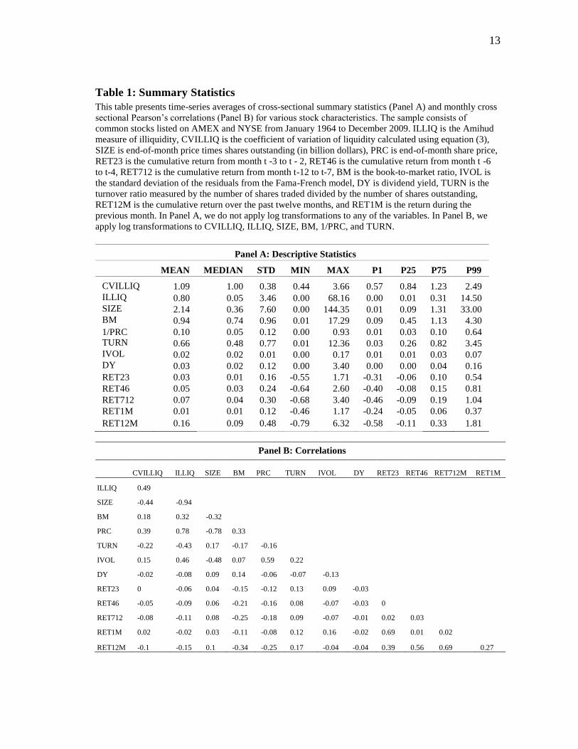
Table 1: Summary Statistics

This table presents time-series averages of cross-sectional summary statistics (Panel A) and monthly cross

sectional Pearson’s correlations (Panel B) for various stock characteristics. The sample consists of

common stocks listed on AMEX and NYSE from January 1964 to December 2009. ILLIQ is the Amihud

measure of illiquidity, CVILLIQ is the coefficient of variation of liquidity calculated using equation (3),

SIZE is end-of-month price times shares outstanding (in billion dollars), PRC is end-of-month share price,

RET23 is the cumulative return from month t -3 to t - 2, RET46 is the cumulative return from month t -6

to t-4, RET712 is the cumulative return from month t-12 to t-7, BM is the book-to-market ratio, IVOL is

the standard deviation of the residuals from the Fama-French model, DY is dividend yield, TURN is the

turnover ratio measured by the number of shares traded divided by the number of shares outstanding,

RET12M is the cumulative return over the past twelve months, and RET1M is the return during the

previous month. In Panel A, we do not apply log transformations to any of the variables. In Panel B, we

apply log transformations to CVILLIQ, ILLIQ, SIZE, BM, 1/PRC, and TURN.

Panel A: Descriptive Statistics

MEAN MEDIAN STD MIN MAX P1 P25 P75 P99

CVILLIQ 1.09 1.00 0.38 0.44 3.66 0.57 0.84 1.23 2.49

ILLIQ 0.80 0.05 3.46 0.00 68.16 0.00 0.01 0.31 14.50 SIZE 2.14 0.36 7.60 0.00 144.35 0.01 0.09 1.31 33.00 BM 0.94 0.74 0.96 0.01 17.29 0.09 0.45 1.13 4.30

1/PRC 0.10 0.05 0.12 0.00 0.93 0.01 0.03 0.10 0.64 TURN 0.66 0.48 0.77 0.01 12.36 0.03 0.26 0.82 3.45 IVOL 0.02 0.02 0.01 0.00 0.17 0.01 0.01 0.03 0.07 DY 0.03 0.02 0.12 0.00 3.40 0.00 0.00 0.04 0.16

RET23 0.03 0.01 0.16 -0.55 1.71 -0.31 -0.06 0.10 0.54

RET46 0.05 0.03 0.24 -0.64 2.60 -0.40 -0.08 0.15 0.81

RET712 0.07 0.04 0.30 -0.68 3.40 -0.46 -0.09 0.19 1.04

RET1M 0.01 0.01 0.12 -0.46 1.17 -0.24 -0.05 0.06 0.37

RET12M 0.16 0.09 0.48 -0.79 6.32 -0.58 -0.11 0.33 1.81

Panel B: Correlations

CVILLIQ ILLIQ SIZE BM PRC TURN IVOL DY RET23 RET46 RET712M RET1M

ILLIQ 0.49

SIZE -0.44 -0.94

BM 0.18 0.32 -0.32

PRC 0.39 0.78 -0.78 0.33

TURN -0.22 -0.43 0.17 -0.17 -0.16

IVOL 0.15 0.46 -0.48 0.07 0.59 0.22

DY -0.02 -0.08 0.09 0.14 -0.06 -0.07 -0.13

RET23 0 -0.06 0.04 -0.15 -0.12 0.13 0.09 -0.03

RET46 -0.05 -0.09 0.06 -0.21 -0.16 0.08 -0.07 -0.03 0

RET712 -0.08 -0.11 0.08 -0.25 -0.18 0.09 -0.07 -0.01 0.02 0.03

RET1M 0.02 -0.02 0.03 -0.11 -0.08 0.12 0.16 -0.02 0.69 0.01 0.02

RET12M -0.1 -0.15 0.1 -0.34 -0.25 0.17 -0.04 -0.04 0.39 0.56 0.69 0.27

14

14

when we write CVILLIQ from now on we are referring to the natural logarithm of the

variable. The same applies for all other variables except IVOL, DY, and return-related

variables.

Panel B of Table 1, we present time-series averages of monthly cross-sectional

Pearson’s correlations. The correlation between SIZE and ILLIQ is -0.94 which is in

line with the evidence that smaller firms are less liquid. We utilize multiple regression

specifications in our empirical analysis to ensure that the results are not contaminated by

this high correlation. The correlation between CVILLIQ and ILLIQ is positive (0.49)

and at a moderate level compared to the correlation (0.93) between SD (DPIOFi,j )t and

ILLIQ. The correlation between the level and volatility of liquidity is similar to the one

reported in CSA when they use the coefficient of variation of dollar volume and turnover

over the past 36 months. In addition, since we use both ILLIQ and CVILLIQ in our

multivariate regressions, the concern that part of the effect of CVILLIQ on future returns

might be due to the correlation of ILLIQ with other variables should be alleviated.

Finally, the correlation between IVOL and CVILLIQ is 0.15, indicating that

these two variables do not capture the same effect even though they both include the

stock return.

15

15

3. EMPIRICAL RESULTS

3.1 Portfolio Approach

We begin the analysis using a portfolio approach where we assign stocks to

portfolios based on the variation of liquidity, CVILLIQ, and other firm characteristics

such as size, illiquidity, momentum, and book-to-market. This is a standard approach,

pioneered by Jegadeesh and Titman (1993), which reduces the variability in returns.

Each month, we assign stocks into 3 categories based on various firm characteristics.

Then we further sort stocks into quintiles based on CVILLIQ. All stocks are held for a

month after skipping a week after portfolio formation. Monthly portfolio returns are

calculated as equally-weighted or value-weighted averages of the returns of all stocks in

the portfolio.

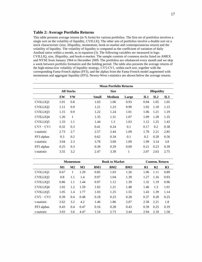
Table 2 present the average returns of portfolios sorted by CVILLIQ alone and

by characteristics and CVILLIQ. The first panel contains the results for the univariate

sort on CVILLIQ using both equal- and value-weighted returns. According to the results,

as CVILLIQ increases the average returns also increase which is in line with the

prediction that stocks with higher volatility of liquidity have higher average returns. The

difference between the highest and lowest CVILLIQ quintiles (CV5-CV1) is 32 basis

points per month for equally-weighted returns. The difference is significant with a t-

statistic of 2.73.

We also calculate the abnormal returns of the high-minus-low volatility of

liquidity strategy (CV5- CV1) using the Fama-French (1993) model. The alpha is 30

16

16

basis points and significant at the 1% level. Similar results hold for value-weighted

returns. When we use the Fama-French model augmented with momentum and

aggregate liquidity, the results are qualitatively identical. In that model, the alpha is

25 basis points and significant at the 1% level.21

In the second panel of Table 2, we first sort stocks into three groups, S1, S2, and

S3 based on SIZE, where S1 represents small stocks and S3 represents large stocks. We

then independently sort stocks into quintiles based on CVILLIQ. The intersection of the

two sorts creates 15 portfolios which are held for a month after skipping a week after

portfolio formation. The results show that the difference between the extreme CVILLIQ

quintiles, CV5 and CV1, decreases as firm size increases. While the difference between

CV5 and CV1 for small stocks is 41 basis points per month and significant, it decreases

to an insignificant 10 basis points per month for large stocks. However, the positive

relation between the volatility of liquidity and returns is not confined to the smallest size

group; it is also present among medium cap stocks.

The Fama-French alpha of the CV5-CV1 strategy is 62 basis points per month

for small stocks. The Fama-French model augmented with momentum and liquidity

yields an alpha of 39 basis points. Overall, the results suggest that the volatility of

liquidity effect is strongest among small stocks.

21

The aggregate liquidity factor is constructed using 9 equally-weighted portfolios sorted on size and

illiquidity. Every month, we sort stocks into 3 groups (Small, Medium, and Big) according to their end of-

previous-month market capitalization. Then we further sort stocks into three groups (High, Medium, and

Low) according to their average monthly Amihud illiquidity. Each portfolio is rebalanced monthly. The

liquidity factor is the average return on three high illiquidity portfolios minus the average return on three

low illiquidity portfolios: ILL =1/3( HighSmall + HighMedium + HighBig )- 1/3 ( LowSmall +

LowMedium + LowBig).

17

17

Table 2: Average Portfolio Returns

This table presents average returns (in % form) for various portfolios. The first set of portfolios involves a

single sort on the volatility of liquidity, CVILLIQ. The other sets of portfolios involve a double sort on a

stock characteristic (size, illiquidity, momentum, book-to-market and contemporaneous return) and the

volatility of liquidity. The volatility of liquidity is computed as the coefficient of variation of daily

Amihud ratios within a month, as in equation (3). The following variables are measured in logs:

CVILLIQ, size, illiquidity, and book-o-market. The sample consists of common stocks listed on AMEX

and NYSE from January 1964 to December 2009. The portfolios are rebalanced every month and we skip

a week between portfolio formation and the holding period. The table also presents the average returns of

the high-minus-low volatility of liquidity strategy, CV5-CV1, within each sort, together with the

corresponding Fama-French alphas (FF3), and the alphas from the Fama-French model augmented with

momentum and aggregate liquidity (FF5). Newey-West t-statistics are shown below the average returns. .

Mean Portfolio Returns

All Stocks

Size

Illiquidity

EW VW

Small Medium Large

IL1 IL2 IL3

CVILLIQ1 1.01 0.8

1.03 1.06 0.93

0.94 1.05 1.05

CVILLIQ2 1.11 0.9

1.21 1.23 0.99

1.02 1.18 1.15

CVILLIQ3 1.15 0.9

1.22 1.24 1.01

1.06 1.21 1.19

CVILLIQ4 1.26 1

1.35 1.31 1.07

1.09 1.28 1.35

CVILLIQ5 1.33 1.1

1.44 1.3 1.03

1.12 1.25 1.43

CV5 − CV1 0.32 0.3

0.41 0.24 0.1

0.17 0.2 0.38

t-statistic 2.73 2.7

2.57 2.44 1.09

1.78 2.21 2.85

FF3 alphas 0.3 0.2

0.62 0.34 0.1

0.2 0.28 0.56

t-statistic 3.04 2.3

3.78 3.69 1.09

1.99 3.14 3.8

FF5 alphas 0.25 0.3

0.39 0.29 0.09

0.21 0.23 0.39

t-statistic 3.55 3.2

2.47 3.39 1

2.07 2.63 2.75

Momentum

Book to Market

Contem. Return

M1 M2 M3

BM1 BM2 BM3

R1 R2 R3

CVILLIQ1 0.67 1 1.29

0.85 1.03 1.26

1.06 1.11 0.89

CVILLIQ2 0.8 1.1 1.4

0.97 1.04 1.39

1.27 1.16 0.93

CVILLIQ3 0.86 1.1 1.44

0.97 1.12 1.39

1.32 1.19 0.96

CVILLIQ4 1.02 1.2 1.59

1.02 1.21 1.48

1.46 1.3 1.01

CVILLIQ5 1.05 1.4 1.77

1.03 1.25 1.55

1.43 1.39 1.14

CV5 − CV1 0.39 0.4 0.48

0.18 0.23 0.28

0.37 0.28 0.25

t-statistic 2.62 3.2 4.2

1.46 1.86 2.07

2.58 2.21 1.8

FF3 alphas 0.43 0.4 0.47

0.16 0.28 0.43

0.39 0.25 0.19

t-statistic 3.03 3.6 4.47

1.54 2.73 3.44

2.94 2.18 1.58

18

18

In the remainder of Table 2, we perform additional double-sorts using control

variables that have been shown to affect returns: illiquidity (ILLIQ), momentum

(RET12M), book- to-market (BM), and contemporaneous return (RET1M). The result

suggest that the average return of the high-minus-low volatility of liquidity strategy

(CV5-CV1) is higher for less liquid stocks (ILL3), value stocks (BM3), and

contemporaneous losers (R1). While past performance over the previous 12 months does

not seem to be related to the volatility of liquidity when we use raw returns or the Fama-

French model, the effect appears to be more pronounced among winners when we use

the Fama-French model augmented with momentum and liquidity.

Overall, the portfolio approach suggests that the positive relation between the

volatility of liquidity and average returns is a separate effect which is different than the

well documented size, momentum and book-to-market effects. In addition, the volatility

of liquidity effect does not seem to be concentrated only among a small portion of the

sample of stocks.

3.2 Regression Approach

In this section we extend the portfolio analysis from before by performing cross-

sectional regressions. These regressions allow us to control for various other stock

characteristics that may potentially affect the relation between the volatility of

liquidity and returns. More precisely, we use Fama-MacBeth (1973) regressions in

which the dependent variables are excess returns. The main independent variable is the

coefficient of variation of illiquidity, CVILLIQ. We adjust the Fama-MacBeth t-

statistics for heteroskedasticity and autocorrelation of up to 8 lags.

19

19

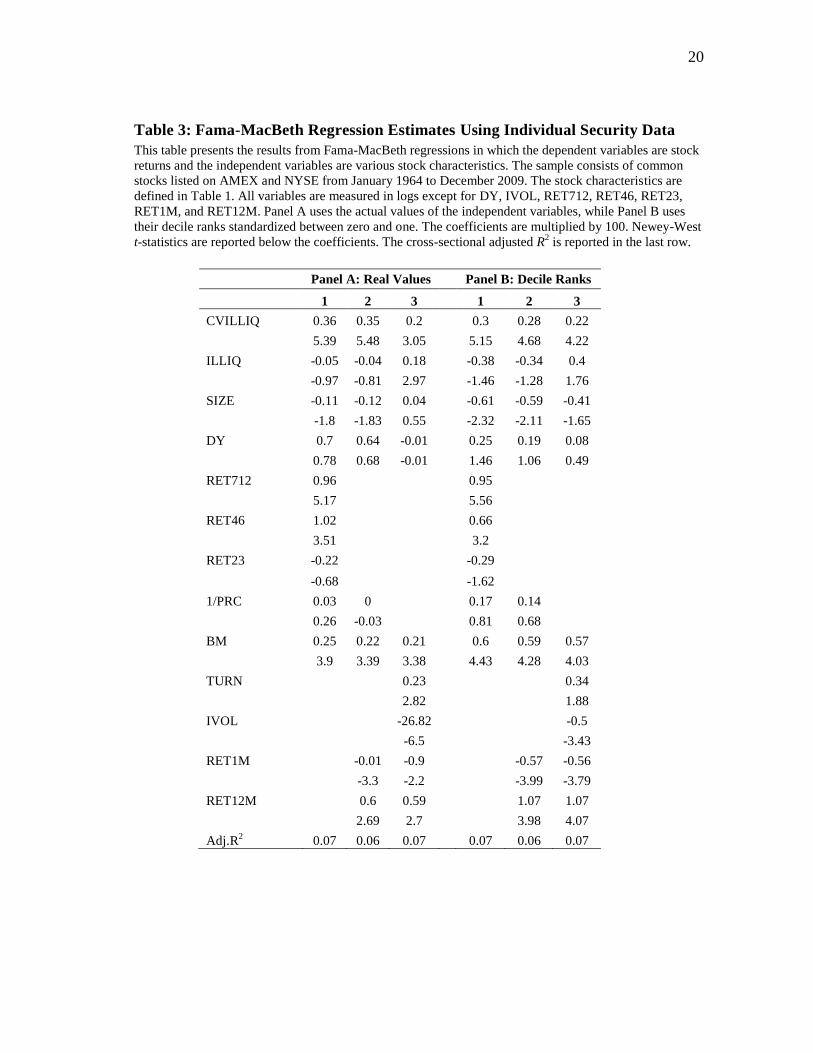
The results are presented in Table 3. Panel A presents results using the real

values of the independent variables. There are three columns in Panel A, each one

corresponding to a different regression specification. In column 1, we use ILLIQ,

SIZE, BM, DY, 1/PRC, RET23, RET46, and RET712. These are the same control

variables as the ones used in CSA. In column 2, we use an alternative set of return

variables, RET12M and RET1M, to control for both past returns and returns

contemporaneous to CVILLIQ. The variable RET1M is included to take into account the

monthly reversal effect documented by Jegadeesh (1990). Since the calculation of

CVILLIQ involves return and volume data, in column 3 of Table 3 we include

idiosyncratic return volatility, IVOL, and turnover, TURN, to the set of control

variables. Price is excluded from the analysis in column 3 since it is highly correlated

with market size, illiquidity, and idiosyncratic volatility. However, the results are not

affected if price is included in the regression.

The results show that CVILLIQ is positively and significantly related to expected

returns in all specifications. The illiquidity level, ILLIQ, is not significant in columns 1

and 2, which may be a result of the presence of both price and size in the same

regression. However, the level of illiquidity is significantly positive in column 3, which

is in line with Amihud and Mendelson (1986) and Amihud (2002). Since ILLIQ and

SIZE are strongly correlated, there might be a potential multicollinearity problem in a

regression that includes both of these variables. In untabulated results, we exclude SIZE

from the model and the coefficient on ILLIQ becomes significantly positive in all

specifications. When we exclude ILLIQ instead, the coefficient on SIZE is significantly

20

20

Table 3: Fama-MacBeth Regression Estimates Using Individual Security Data

This table presents the results from Fama-MacBeth regressions in which the dependent variables are stock

returns and the independent variables are various stock characteristics. The sample consists of common

stocks listed on AMEX and NYSE from January 1964 to December 2009. The stock characteristics are

defined in Table 1. All variables are measured in logs except for DY, IVOL, RET712, RET46, RET23,

RET1M, and RET12M. Panel A uses the actual values of the independent variables, while Panel B uses

their decile ranks standardized between zero and one. The coefficients are multiplied by 100. Newey-West

t-statistics are reported below the coefficients. The cross-sectional adjusted R2 is reported in the last row.

Panel A: Real Values

Panel B: Decile Ranks

1 2 3

1 2 3

CVILLIQ 0.36 0.35 0.2

0.3 0.28 0.22

5.39 5.48 3.05

5.15 4.68 4.22

ILLIQ -0.05 -0.04 0.18

-0.38 -0.34 0.4

-0.97 -0.81 2.97

-1.46 -1.28 1.76

SIZE -0.11 -0.12 0.04

-0.61 -0.59 -0.41

-1.8 -1.83 0.55

-2.32 -2.11 -1.65

DY 0.7 0.64 -0.01

0.25 0.19 0.08

0.78 0.68 -0.01

1.46 1.06 0.49

RET712 0.96

0.95

5.17

5.56

RET46 1.02

0.66

3.51

3.2

RET23 -0.22

-0.29

-0.68

-1.62

1/PRC 0.03 0

0.17 0.14

0.26 -0.03

0.81 0.68

BM 0.25 0.22 0.21

0.6 0.59 0.57

3.9 3.39 3.38

4.43 4.28 4.03

TURN

0.23

0.34

2.82

1.88

IVOL

-26.82

-0.5

-6.5

-3.43

RET1M

-0.01 -0.9

-0.57 -0.56

-3.3 -2.2

-3.99 -3.79

RET12M

0.6 0.59

1.07 1.07

2.69 2.7

3.98 4.07

Adj.R2 0.07 0.06 0.07

0.07 0.06 0.07

21

21

negative in all specifications. The relation between return and the volatility of liquidity is

not affected by these modifications.

Note that the coefficient on turnover has a positive sign in the third specification.

This result differs from the findings of CSA who show that TURN has a negative effect

on expected returns. In untabulated tests we find that the coefficient on TURN becomes

negative once CVILLIQ, ILLIQ, and IVOL are excluded from the regression. Turnover

is used in the literature as a proxy for liquidity or divergence of opinion among

investors. Since ILLIQ and IVOL are such proxies as well, it is possible that the positive

coefficient on TURN in model 3 is a result of the interaction between all these variables.

To ensure that our results are not driven by this interaction, we repeat the analysis within

different turnover groups and find similar results.

Instead of using the real values of the independent variables, in Panel B of Table

3 we first transform the independent variables into decile ranks and then standardize the

ranks with values between zero and one. This rank transformation has two advantages:

it makes the coefficient interpretation more intuitive and comparable across variables,

and it minimizes the effect of outlier observations. Panel B shows that the results are

similar and somewhat stronger compared to the results in Panel A. The results in column

3 suggest that, after controlling for various firm characteristics, stocks in the highest

CVILLIQ decile earn on average 22 basis points per month more than stocks in the

lowest CVILLIQ decile.

Overall, the results in Table 3 suggest that the volatility of liquidity is

significantly positively related to average returns. This relation persists over and above

22

22

the positive correlation between the level of illiquidity and returns. This is in line with

the hypothesis that investors want to be compensated for holding stocks whose liquidity

is more volatile.

3.3 Regression Approach within Size and Illiquidity Groups

As mentioned earlier, the high correlation between size and illiquidity may cause

potential multicollinearity problems and bias our results. In this section we perform

additional tests to ensure that the main results are not driven by this correlation. Every

month we sort stocks based on size or illiquidity and run Fama-MacBeth regression

within each size or illiquidity group. This way we control for one of the correlated

variables and allow the other one to vary within each group. For the sake of brevity we

repot the results using the 3rd model from our previous analysis, but the results are

similar for models 1 and 2.

In Panel A of Table 4, we report Fama-MacBeth regressions within each size

category. The results suggest that the positive relation between CVILLIQ and returns is

stronger among smaller stocks. Furthermore, the level of illiquidity is significant and

positive in all size groups. When we move from larger to smaller stocks, the volatility of

liquidity and the illiquidity effects get stronger. Overall, the results suggest that, after

controlling for the size effect, both the mean and the second moment of illiquidity are

positively related to expect stock returns.

23

Table 4: Fama-MacBeth Regression Estimates by Size and Illiquidity Groups This table presents the results from Fama-MacBeth regressions in which the dependent variables are stock returns and the independent variables are

various stock characteristics. The sample consists of common stocks listed on AMEX and NYSE from January 1964 to December 2009. The stock

characteristics are defined in Table 1. All variables are measured in logs except for DY, IVOL, RET1M, and RET12M. Panel A shows results within

three separate size groups, while Panel B displays results within three separate illiquidity groups. In both panels the actual values or the decile ranks of

the independent variables are used. The coefficients are multiplied by 100. Newey-West t-statistics are reported below the coefficients. The cross-

sectional adjusted R2 is reported in the last row

Panel A: Regressions by Size Group

Panel B: Regressions by Illiquidity Group

Real Values

Decile Ranks

Real Values

Decile Ranks

Small Med. Large

Small Med. Large

ILLIQ1 ILLIQ2 ILLIQ3

ILLIQ1 ILLIQ2 ILLIQ3

CVILLIQ 0.34 0.15 0.08

0.55 0.11 0.06

0.13 0.13 0.52

0.1 0.11 0.65

3.06 1.76 0.98

4.79 1.59 0.95

1.39 1.66 5.15

1.32 1.69 5.92

ILLIQ 0.33 0.14 0.08

1.52 0.67 0.67

5.95 2.81 2.39

2.86 2.53 2.49

SIZE

-0.07 -0.09 -0.3

-0.57 -0.42 -1.02

-1.65 -1.77 -5.05

-1.61 -1.82 -2.98

DY -1.88 -0.22 2.02

-0.05 0.06 0.36

1.3 -0.08 -1.55

0.32 0.07 0.04

-1.2 -0.17 1.42

-0.27 0.33 1.83

0.96 -0.08 -0.83

1.66 0.4 0.21

BM 0.3 0.18 0.06

0.9 0.42 0.22

0.05 0.17 0.31

0.19 0.43 0.87

3.78 2.55 0.84

4.61 2.7 1.4

0.62 2.3 4.12

1.13 2.66 4.77

TURN 0.35 0.2 0.15

0.56 0.5 0.47

0.04 0.12 0.09

0.25 0.28 0.34

4.36 2.65 2.27

1.71 2.77 2.72

0.55 2.01 1.32

1.51 1.96 1.09

IVOL -32.98 -29.67 -20.8

-0.89 -0.5 -0.3

-21.49 -29.03 -22.93

-0.31 -0.49 -0.63

-7.75 -5.87 -3.17

-4.52 -3.49 -1.79

-3.31 -5.93 -5.17

-1.9 -3.08 -3.08

RET1M -1.02 -0.42 -1.44

-0.61 -0.43 -0.62

-0.72 0.11 -1.53

-0.43 -0.4 -0.72

-2.06 -0.88 -2.69

-3.14 -2.78 -4.16

-1.22 0.24 -3.07

-2.72 -2.54 -3.73

RET12M 0.81 0.49 0.6

1.54 0.94 0.73

0.49 0.44 0.94

0.79 0.93 1.49

3.99 1.97 2.36

5.42 3.41 2.7

1.94 1.68 4.61

2.86 3.3 5.41

Adj.R2 0.04 0.06 0.1

0.04 0.06 0.1

0.11 0.07 0.04

0.11 0.06 0.04

24

24

In Panel B of Table 4, the Fama-MacBeth regressions are performed within

each illiquidity category. The coefficient on CVILLIQ is positive and significant among

the less liquid stocks. The significance level of the CVILLIQ coefficient decreases as

liquidity increases, but it still remains positive among the most liquid stocks. A

similar pattern is observed for the SIZE coefficient as the sign is negative for all

illiquidity groups but significant only among the least liquid stocks (ILLIQ3). Once

again the results are similar if the independent variables are measured in decile ranks.

One notable observation is that CVILLIQ is more significant among small and

illiquid stocks. A possible explanation might be that illiquid stocks have low average

levels of liquidity and therefore, a high volatility of the liquidity distribution implies that

investors in illiquid stocks may face even lower levels of liquidity at a point when they

need to trade. Liquid stocks, on the other hand, may expose investors to this risk to a

lower extent since their liquidity distributions have higher means.

Overall, the results in Table 4 suggest that our previous findings are not driven

by multicollinearity biases due to the high correlation between size and illiquidity.

Controlling for this correlation, the coefficient on CVILLIQ is still positive and

significant.

25

25

4. ROBUSTNESS

4.1 Risk Adjusted Returns

The Fama-MacBeth regressions that we run previously use non-risk-adjusted

excess returns as the dependent variables and relate them to the volatility of liquidity and

other firm characteristics. Since we do not control for systematic risk, it might be

possible that our previous results are driven by exposure to some well-known risk

factors. In order to control for this possibility, we follow Brennan, Chordia, and

Subrahmanyam (1998) and examine the relation between risk-adjusted returns and the

volatility of liquidity. The risk-adjustment is done relative to the Fama-French model

augmented with momentum and aggregate liquidity. It is important to control for

exposure to aggregate liquidity since previous studies have shown that return sensitivity

to market liquidity is priced (e.g., Pastor and Stambaugh (2003)). Factor loadings are

estimated using a 60-month rolling window and the Dimson (1979) procedure with one

lag is used to adjust the estimated factor loadings for possible thin trading.22

In addition, previous studies have shown that asset liquidity changes over time

and this time variation is governed by a significant common component in the liquidity

across assets (see, e.g., Chordia, Roll, and Subrahmanyam (2000), Hasbrouck and

Seppi (2001), Amihud (2002), and Korajczyk and Sadka (2008)). Therefore, the

volatility of liquidity for a given stock might be driven by exposure to aggregate market

liquidity or the aggregate market return. Therefore, it is possible that our measure of the

22

The results are not sensitive to using the Dimson (1979) adjustment. We also use the Fama-French

three-factor model to adjust for risk and obtain similar results.

26

26

volatility of liquidity captures the risk associated with the covariance of a stock’s

liquidity with aggregate market liquidity or the market return (see Acharya and Pederson

(2005)). If a stock becomes illiquid when the market as a whole is illiquid, investors

would like to be compensated for holding this security. Furthermore, if a stock becomes

illiquid if the market overall is doing badly, then this security will require a higher

expected return as well. To address these two covariance effects, we include two

additional variables in our regressions. These variables are a stock’s illiquidity

sensitivity to aggregate market illiquidity, βL,L, and its sensitivity to the market return,

βL,M. The betas for each stock are derived from a regression of the stocks illiquidity on

the market illiquidity and the market return using daily data within a month.23

Aggregate market illiquidity is calculated as the equally-weighted average of stocks’

daily illiquidity measures. If our volatility of liquidity measure, CVILLIQ, captures the

covariance between the assets’s illiquidity and aggregate market illiquidity, or the asset’s

illiquidity and the market return, then the coefficient on CVILLIQ should be

insignificant in the presence of βL,L and βLM.

Table 5 presents the results from risk-adjusted Fama-MacBeth regressions.

Panel A contains the coefficients from standard Fama-MacBeth regressions with real

values of the independent variables, Panel B shows the coefficients from standard

Fama-MacBeth regressions with decile ranks of the independent variables, and Panel

C presents purged estimators.

23

We obtain similar results if the sensitivities are derived from univariate regressions.

27

27

Table 5: Fama-MacBeth Regression Estimates: Using Risk-Adjusted Returns as

the Dependent Variables

This table presents the results from Fama-MacBeth regressions in which the dependent variables are risk-

adjusted returns and the independent variables are various stock characteristics. The risk-adjustment is

based on the Fama-French model augmented with momentum and aggregate liquidity and the Dimson

procedure with one lag. βL,L and βL,M are the respective coefficient estimates from monthly multivariate

regressions of daily firm-level Amihud measures on daily aggregate Amihud measures and daily market

returns within each month. The label ”Raw” in Panel A refers to the standard Fama-MacBeth coefficients,

the label ”Decile” in Panel B refers to the decile ranks of the Fama-MacBeth coefficients, while the label

”Purged” in Panel C refers to the intercept terms from time-series regressions of the Fama-MacBeth

coefficients on the factors. The sample consists of common stocks listed on AMEX and NYSE from

January 1964 to December 2009. The stock characteristics are defined in Table 1. All variables are

measured in logs except for DY, IVOL, RET1M, RET12M, βL,L and βL,M . The coefficients are multiplied

by 100. Newey-West t-statistics are reported below the coefficients. The cross-sectional adjusted R2 is

reported in the last row.

Panel A: Raw

Panel B: Decile

Panel C: Purged

1 2

1 2

1 2

CVILLIQ 0.21 0.19

0.24 0.24

0.19 0.18

2.99 2.65

3.81 3.88

2.28 2.1

βL,L

0

0.07

0

-0.27

1.3

-0.18

βL,M

-275.21

-0.17

-302.16

-0.77

-2.72

-0.79

ILLIQ 0.2 0.19

0.22 0.17

0.19 0.18

3.49 3.21

0.97 0.76

2.61 2.32

SIZE 0.09 0.08

-0.34 -0.36

0.07 0.06

1.42 1.21

-1.5 -1.58

0.92 0.74

DY 0.16 0.18

0.13 0.13

0.29 0.29

0.28 0.3

1.17 1.21

0.42 0.43

BM 0.12 0.12

0.34 0.33

0.03 0.03

2.87 2.92

3.28 3.22

0.76 0.8

TURN 0.21 0.2

0.16 0.15

0.22 0.22

2.69 2.6

1.02 0.97

2.31 2.18

IVOL -26.54 -27.53

-0.48 -0.48

-28.51 -29.21

-6.49 -6.8

-3.98 -4.01

-6.77 -6.99

RET1M -2.37 -2.38

-1.05 -1.03

-3.19 -3.2

-4.42 -4.44

-4.74 -4.71

-5.26 -5.26

RET12M 0.37 0.37

0.61 0.61

0.24 0.24

2.15 2.14

2.33 2.33

1.27 1.26

Adj.R2 0.03 0.04

0.03 0.03

28

28

The purged estimators are computed as the constant terms from OLS regressions

of monthly Fama-MacBeth coefficient estimates on factor returns. Each Panel uses two

specifications: the third model from Table 3 and the same model augmented with βL,L

and βL,M.24

According to the results, the coefficient on CVILLIQ remains positive and

significant in all panels of Table 5.

Acharya and Pederson (2005) find that the covariance between an asset’s

illiquidity and the market return is significantly negatively related to stock returns. This

is the case since investors are willing to accept a lower expected return on a security that

is less illiquid in a down market. The results in Table 5 on βL,M are consistent with

Acharya and Pederson (2005). However, βL,M is significant only when the decile ranks

of the independent variables are used. A possible explanation behind the insignificant

coefficient on βL,M in Panels A and C could be the presence of considerable skewness in

the cross-sectional distribution of βL,M.

Overall, the results in table 5 suggest that the volatility of liquidity does not

simply capture the covariance between individual stock liquidity and aggregate market

liquidity or return. To the extent that βL,L and βL,M measure systematic liquidity risk, the

separate pricing of CVILLIQ indicates that idiosyncratic volatility risk is important in

the cross- section of returns. The coefficient on CVILLIQ remains significantly positive

under various risk adjustments and control variables, indicating that it captures an effect

different from a stock’s return (or liquidity) exposure to aggregate liquidity or other

standard return factors.

24

The results are similar for other sets of control variables.

29

29

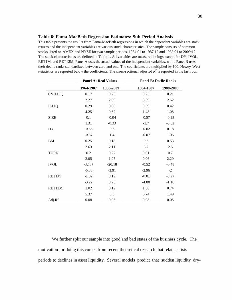
4.2 Sub-Sample Analysis

In this section we examine whether the results are robust across different sample

periods. We divide the sample in two periods, before and after 1987. The motivation for

choosing 1987 comes from Amihud, Mendelson and Wood (1990) who argue that

investors’ perception of illiquidity have changed drastically after the crash of October

1987 and investors have realized that markets are not as liquid as before the crash.

Panel A of Table 6 presents results using the real values of the independent variables,

while Panel B presents results using decile ranks. The two sample periods are from

1964:01 to 1987:12 and from 1988:01 to 2009:12. Panel A, shows that the coefficient on

CVILLIQ is significant and positive in both sub-periods when using the real values of

the independent variables. Panel B shows that the same result holds when we use decile

ranks for the variables.

An interesting observation from Panel A of Table 6 is that illiquidity is positively

related to returns in both sample periods, but it is significant only during the 1964:01 to

1987:12 period. When we exclude size from our analysis to control for

multicollinearity, illiquidity becomes significant in the later period but the effect is

relatively weaker compared to the earlier period. 25

Overall, the results suggest that the

volatility of liquidity is significantly related to average returns in both time periods that

we examine.

25

Ben-Raphael, Kadan, and Wohl (2009) show that both the sensitivity of stock returns to illiquidity and

the illiquidity premia have declined over the past four decades. They claim that the proliferation of index

funds and exchange-traded funds, and enhancements in markets that facilitate arbitrage activity might

explain their results.

30

30

Table 6: Fama-MacBeth Regression Estimates: Sub-Period Analysis This table presents the results from Fama-MacBeth regressions in which the dependent variables are stock

returns and the independent variables are various stock characteristics. The sample consists of common

stocks listed on AMEX and NYSE for two sample periods, 1964:01 to 1987:12 and 1988:01 to 2009:12.

The stock characteristics are defined in Table 1. All variables are measured in logs except for DY, IVOL,

RET1M, and RET12M. Panel A uses the actual values of the independent variables, while Panel B uses

their decile ranks standardized between zero and one. The coefficients are multiplied by 100. Newey-West

t-statistics are reported below the coefficients. The cross-sectional adjusted R2 is reported in the last row.

Panel A: Real Values

Panel B: Decile Ranks

1964-1987 1988-2009 1964-1987 1988-2009

CVILLIQ 0.17 0.23

0.23 0.21

2.27 2.09

3.39 2.62

ILLIQ 0.29 0.06

0.39 0.42

4.25 0.62

1.48 1.08

SIZE 0.1 -0.04

-0.57 -0.23

1.31 -0.33

-1.7 -0.62

DY -0.55 0.6

-0.02 0.18

-0.37 1.4

-0.07 1.06

BM 0.25 0.18

0.6 0.53

2.63 2.11

3.2 2.5

TURN 0.2 0.27

0.01 0.7

2.05 1.97

0.06 2.29

IVOL -32.87 -20.18

-0.52 -0.48

-5.33 -3.91

-2.96 -2

RET1M -1.82 0.12

-0.81 -0.27

-3.22 0.23

-4.88 -1.16

RET12M 1.02 0.12

1.36 0.74

5.37 0.3

6.74 1.49

Adj.R2 0.08 0.05

0.08 0.05

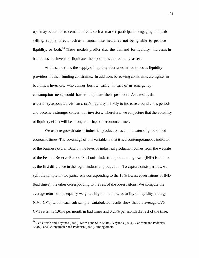
We further split our sample into good and bad states of the business cycle. The

motivation for doing this comes from recent theoretical research that relates crisis

periods to declines in asset liquidity. Several models predict that sudden liquidity dry-

31

31

ups may occur due to demand effects such as market participants engaging in panic

selling, supply effects such as financial intermediaries not being able to provide

liquidity, or both.26

These models predict that the demand for liquidity increases in

bad times as investors liquidate their positions across many assets.

At the same time, the supply of liquidity decreases in bad times as liquidity

providers hit their funding constraints. In addition, borrowing constraints are tighter in

bad times. Investors, who cannot borrow easily in case of an emergency

consumption need, would have to liquidate their positions. As a result, the

uncertainty associated with an asset’s liquidity is likely to increase around crisis periods

and become a stronger concern for investors. Therefore, we conjecture that the volatility

of liquidity effect will be stronger during bad economic times.

We use the growth rate of industrial production as an indicator of good or bad

economic times. The advantage of this variable is that it is a contemporaneous indicator

of the business cycle. Data on the level of industrial production comes from the website

of the Federal Reserve Bank of St. Louis. Industrial production growth (IND) is defined

as the first difference in the log of industrial production. To capture crisis periods, we

split the sample in two parts: one corresponding to the 10% lowest observations of IND

(bad times), the other corresponding to the rest of the observations. We compute the

average return of the equally-weighted high-minus-low volatility of liquidity strategy

(CV5-CV1) within each sub-sample. Untabulated results show that the average CV5-

CV1 return is 1.01% per month in bad times and 0.23% per month the rest of the time.

26

See Gromb and Vayanos (2002), Morris and Shin (2004), Vayanos (2004), Garleanu and Pedersen

(2007), and Brunnermeier and Pedersen (2009), among others.

32

32

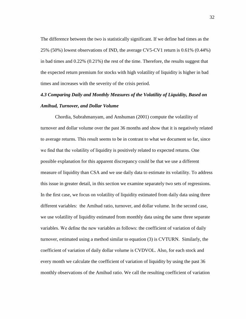
The difference between the two is statistically significant. If we define bad times as the

25% (50%) lowest observations of IND, the average CV5-CV1 return is 0.61% (0.44%)

in bad times and 0.22% (0.21%) the rest of the time. Therefore, the results suggest that

the expected return premium for stocks with high volatility of liquidity is higher in bad

times and increases with the severity of the crisis period.

4.3 Comparing Daily and Monthly Measures of the Volatility of Liquidity, Based on

Amihud, Turnover, and Dollar Volume

Chordia, Subrahmanyam, and Anshuman (2001) compute the volatility of

turnover and dollar volume over the past 36 months and show that it is negatively related

to average returns. This result seems to be in contrast to what we document so far, since

we find that the volatility of liquidity is positively related to expected returns. One

possible explanation for this apparent discrepancy could be that we use a different

measure of liquidity than CSA and we use daily data to estimate its volatility. To address

this issue in greater detail, in this section we examine separately two sets of regressions.

In the first case, we focus on volatility of liquidity estimated from daily data using three

different variables: the Amihud ratio, turnover, and dollar volume. In the second case,

we use volatility of liquidity estimated from monthly data using the same three separate

variables. We define the new variables as follows: the coefficient of variation of daily

turnover, estimated using a method similar to equation (3) is CVTURN. Similarly, the

coefficient of variation of daily dollar volume is CVDVOL. Also, for each stock and

every month we calculate the coefficient of variation of liquidity by using the past 36

monthly observations of the Amihud ratio. We call the resulting coefficient of variation

33

33

CVILLIQ36 to distinguish it from our previous measure CVILLIQ which is computed

using daily data within a month. The coefficient of variation of monthly turnover over

the last 36 months is CVTURN36, and the coefficient of variation of monthly dollar

volume over the last 36 months is CVDVOL36. The last two variables are the ones used

by CSA to document a negative relation between the volatility of liquidity and average

returns.

The results are presented in Table 7. As before, we apply log transformations to

the newly defined variables since they exhibit skewness. We use the same control

variables as before. In Panel A the volatility of liquidity is estimated with daily data, in

Panel B it is estimated with monthly data, while in Panel C it is estimated with both

daily and monthly data. For the sake of brevity, we use only one specification in terms of

control variables; however, the results are similar under different specifications.

According to the results in Panel A, the coefficient on CVILLIQ is positive and

significant in the presence of CVTURN or CVDVOL. The coefficient of variation of

daily turnover and dollar volume are negatively related to average returns, but the effect

is not significant in the presence of CVILLIQ.

The results in Panel A suggest that investors fear volatility in the daily price

impact of trade. Therefore, the difference between CSA’s and our results could stem

from using the price impact as a measure of liquidity and also estimating the volatility

of liquidity using daily data within a month. The volatility of the daily price impact is

associated with a positive return premium. We conjecture that the reason for this is that

traders who have immediate liquidity needs cannot time their trades so that they occur

34

34

only during periods of low price impact. The more volatile the price impact of trade, the

higher is the probability that an immediate liquidity need might be executed at low levels

of liquidity.

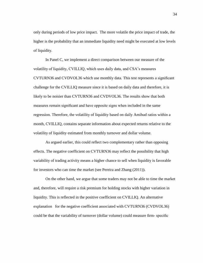
In Panel C, we implement a direct comparison between our measure of the

volatility of liquidity, CVILLIQ, which uses daily data, and CSA’s measures

CVTURN36 and CVDVOL36 which use monthly data. This test represents a significant

challenge for the CVILLIQ measure since it is based on daily data and therefore, it is

likely to be noisier than CVTURN36 and CVDVOL36. The results show that both

measures remain significant and have opposite signs when included in the same

regression. Therefore, the volatility of liquidity based on daily Amihud ratios within a

month, CVILLIQ, contains separate information about expected returns relative to the

volatility of liquidity estimated from monthly turnover and dollar volume.

As argued earlier, this could reflect two complementary rather than opposing

effects. The negative coefficient on CVTURN36 may reflect the possibility that high

variability of trading activity means a higher chance to sell when liquidity is favorable

for investors who can time the market (see Pereira and Zhang (2011)).

On the other hand, we argue that some traders may not be able to time the market

and, therefore, will require a risk premium for holding stocks with higher variation in

liquidity. This is reflected in the positive coefficient on CVILLIQ. An alternative

explanation for the negative coefficient associated with CVTURN36 (CVDVOL36)

could be that the variability of turnover (dollar volume) could measure firm- specific

35

35

Table 7: Fama-MacBeth Regression Estimates: Comparing Daily and Monthly

Measures of the Volatility of Liquidity Based on Amihud, Turnover, and Dollar

Volume This table presents the results from Fama-MacBeth regressions in which the dependent variables are stock

returns and the independent variables are various stock characteristics. The sample consists of common

stocks listed on NYSE and AMEX for the period from January 1964 to December 2009. The stock

characteristics are defined in Table 1. The volatility of liquidity is measured in six separate ways: the

coefficient of variation of daily Amihud ratios within a month (CVILLIQ), the coefficient of variation of

daily turnover within a month (CVTURN), the coefficient of variation of daily dollar volume within a

month (CVDVOL), the coefficient of variation of monthly Amihud ratios over the last 36 months

(CVILLIQ36), the coefficient of variation of monthly turnover over the last 36 months (CVTURN36), and

the coefficient of variation of monthly dollar volume over the last 36 months (CVDVOL36). Panel A

contains only daily measures of the volatility of liquidity, while Panel B contains only monthly measures

of the volatility of liquidity. Panel C contains both. All variables are measured in logs except for DY,

IVOL, RET1M, and RET12M. The coefficients are multiplied by 100. Newey-West t-statistics are

reported below the coefficients. The cross-sectional adjusted R2 is reported in the last row.

Panel A: Daily Panel B: Monthly Panel C: Daily and Monthly

1 2

1 2

1 2

CVILLIQ 0.17 0.18 CVILLIQ36 0.04 0.04 CVILLIQ 0.17 0.17

2.85 2.98

0.37 0.36

2.86 2.84

CVTURN -0.08

CVTURN 36 -0.26

CVTURN 36 -0.27

-1.08

-4.15

-4.4

CVDVOL

-0.13 CVDVOL36

-0.15 CVDVOL36

-0.15

-1.72

-2.06

-1.96

ILLIQ 0.22 0.24 ILLIQ 0.21 0.21 ILLIQ 0.2 0.2

2.94 3.13

3.56 3.52

3.1 3.09

SIZE 0.08 0.08 SIZE 0.03 0.04 SIZE 0.03 0.04

1.04 1.16

0.43 0.57

0.39 0.5

DY 0.1 0.1 DY -0.05 -0.06 DY 0.1 0.09

0.13 0.14

-0.06 -0.08

0.14 0.13

BM 0.19 0.19 BM 0.18 0.18 BM 0.19 0.19

3.13 3.13

3.08 3.09

3.09 3.11

TURN 0.26 0.27 TURN 0.25 0.25 TURN 0.25 0.25

2.65 2.77

3.35 3.39

2.86 2.9

IVOL -25.4 -25.5 IVOL -25.2 -25.21 IVOL -24.4 -24.37

-6.12 -6.11

-5.88 -5.93

-5.56 -5.63

RET1M -0.88 -0.86 RET1M -0.9 -0.9 RET1M -0.87 -0.88

-2.09 -2.07

-2.18 -2.18

-2.08 -2.09

RET12M 0.58 0.58 RET12M 0.61 0.61 RET12M 0.6 0.59

2.7 2.7

3.1 3.06

2.71 2.66

Adj.R2 0.07 0.07 Adj.R

2 0.07 0.07 Adj.R

2 0.07 0.07

36

36

negative relation between the variability of trading activity and returns. He shows that at

the firm level, high variability of turnover implies high uncertainty and low aggregate

volatility risk. Therefore, firms with high variability of turnover beat the CAPM in

periods of increasing market variance and this explains their low expected returns.

Other studies that use turnover as a proxy for firm-specific uncertainty or investor

disagreement include Harris and Raviv (1993) and Blume, Easley, and O’Hara (1994),

among others. Turnover is found to be high if prices fluctuate a lot, if traders disagree

about firm value, or if they receive a lot of information about the firm (e.g., Karpoff

(1987)). On the other hand, the effect of volume on returns is ambiguous. While CSA

find a negative relations, Gervais, Kaniel and Milgelgrin (2001) documents that unusual

volume is positively related to future returns.

Alternatively, CSA’s findings might be related to short sale restrictions. We

explain this potential relation below. High volatility of trading activity might be related

to an increase in investor disagreement. On the other hand, high volatility of trading

activity might be due to high volume shocks which attract investors’ attention. If a

certain stock experiences an increase in investor disagreement or if it attracts the

attention of investors, under short sale restrictions the price of the stock will reflect the

views of optimistic investors and this will lead to overvaluation as argued by Miller

(1977). Since the overvaluation would be temporary, the price will converge to its

fundamental value as the uncertainty about the stock is resolved. Therefore, the

documented negative relation between the volatility of trading and returns might be a

result of overvaluation. In that case, we would expect that the result documented by CSA

37

37

would be stronger among stocks with high short sale restrictions. We test this

hypothesis below.

We measure short sale restrictions using residual institutional ownership

(RESIO), following Nagel (2005). Data on institutional ownership are obtained from 13-

F filings, available from Thomson Financial for the period 1980-2009. We define

Institutional Ownership (IO), as the sum of the holdings of all institutions for each stock

in each quarter, divided by the number of shares outstanding obtained from CRSP.

Stocks that have available return data but no reported institutional holdings are assumed

to have zero institutional ownership. IO values below 0.0001 and above 0.9999 are

replaced with 0.0001 and 0.9999, respectively. Following Nagel (2005), every quarter

we regress the logit transformation of institutional ownership of each stock on log

(SIZE) and log (SIZE)2. Next we average the slope coefficients of the independent

variables over time. The residuals of the regressions stand for Residual Institutional

Ownership (RESIO). We average the residual IO for each stock over the course of the

past ten quarters to obtain average residual IO. Following Nagel (2005), RESIO is

lagged two quarters so that the results are not driven by the short- term outperformance

of institutional investors’ trades (see Chen, Jegadeesh, and Wermers (2000) and Yan and

Zhang (2009)). We divide stocks in two groups according to high and low RESIO, and

we run Fama-McBeth regressions within each group. Our measure of the volatility of

liquidity, CVILLIQ, and CSA’s measure are both included in each regression. The

results are presented in table 8.

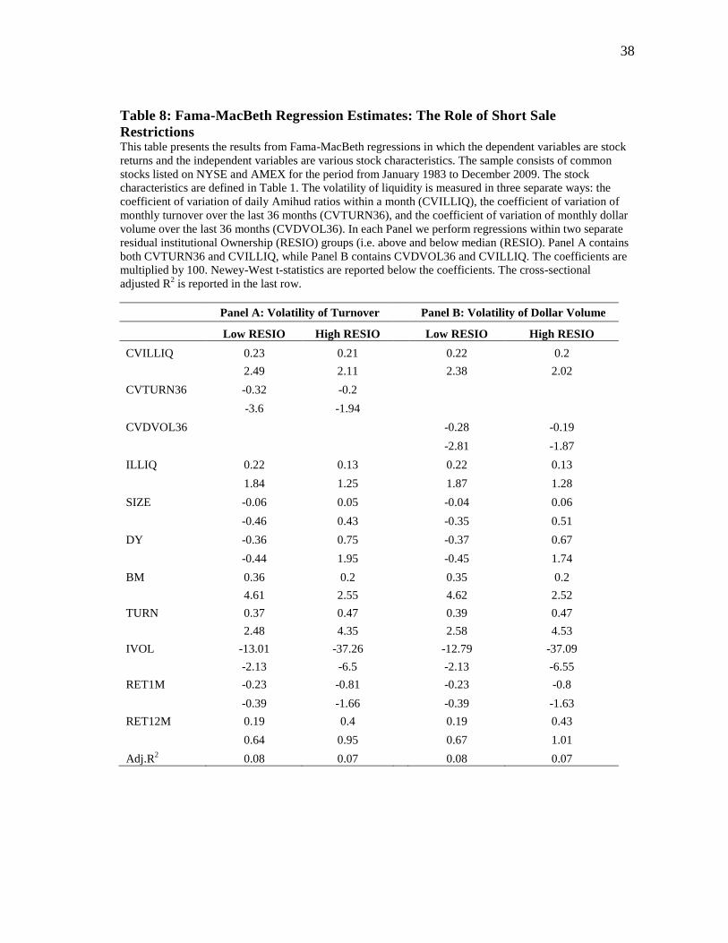
38

38

Table 8: Fama-MacBeth Regression Estimates: The Role of Short Sale

Restrictions This table presents the results from Fama-MacBeth regressions in which the dependent variables are stock

returns and the independent variables are various stock characteristics. The sample consists of common

stocks listed on NYSE and AMEX for the period from January 1983 to December 2009. The stock

characteristics are defined in Table 1. The volatility of liquidity is measured in three separate ways: the

coefficient of variation of daily Amihud ratios within a month (CVILLIQ), the coefficient of variation of

monthly turnover over the last 36 months (CVTURN36), and the coefficient of variation of monthly dollar

volume over the last 36 months (CVDVOL36). In each Panel we perform regressions within two separate

residual institutional Ownership (RESIO) groups (i.e. above and below median (RESIO). Panel A contains

both CVTURN36 and CVILLIQ, while Panel B contains CVDVOL36 and CVILLIQ. The coefficients are

multiplied by 100. Newey-West t-statistics are reported below the coefficients. The cross-sectional

adjusted R2 is reported in the last row.

Panel A: Volatility of Turnover

Panel B: Volatility of Dollar Volume

Low RESIO High RESIO

Low RESIO High RESIO

CVILLIQ 0.23 0.21

0.22 0.2

2.49 2.11

2.38 2.02

CVTURN36 -0.32 -0.2

-3.6 -1.94

CVDVOL36

-0.28 -0.19

-2.81 -1.87

ILLIQ 0.22 0.13

0.22 0.13

1.84 1.25

1.87 1.28

SIZE -0.06 0.05

-0.04 0.06

-0.46 0.43

-0.35 0.51

DY -0.36 0.75

-0.37 0.67

-0.44 1.95

-0.45 1.74

BM 0.36 0.2

0.35 0.2

4.61 2.55

4.62 2.52

TURN 0.37 0.47

0.39 0.47

2.48 4.35

2.58 4.53

IVOL -13.01 -37.26

-12.79 -37.09

-2.13 -6.5

-2.13 -6.55

RET1M -0.23 -0.81

-0.23 -0.8

-0.39 -1.66

-0.39 -1.63

RET12M 0.19 0.4

0.19 0.43

0.64 0.95

0.67 1.01

Adj.R2 0.08 0.07

0.08 0.07

39

39

Table 8 shows that the negative relationship between the volatility of trading

activity over the past 36 months and returns is more pronounced among stocks with high

short sale restrictions. While the coefficient on CVTURN36 is -0.32 in the low RESIO

group and it increases to -0.20 in the high RESIO group. The difference between the two

coefficients is significant at the 1% level. On the other hand, the coefficient on CVILLIQ

is significant in both groups and similar in magnitude across groups. Similar results hold

when the volatility of trading activity is measured by CVDOL36. Overall these results

suggest that CSA’s findings might be related to overvaluation under short sale

restrictions. This is consistent with the argument proposed by Miller (1977).

4.4 Alternative Measurement Periods for the Volatility of Liquidity

So far our results are based on the volatility of liquidity measured from daily data

within a month. However, since the Amihud ratio includes returns, it might be the case

that our measure is capturing some short-term return autocorrelations that cannot be

adjusted for with our control variables. In addition, it might be possible to get more

precise estimates of the volatility of liquidity by using a larger sample of daily Amihud

ratios. Therefore, in this section we investigate whether our results are robust to

alternative measurement periods for our key variable, CVILLIQ.

We use 3, 6, 9, and 12 months of daily Amihud ratios to compute four alternative

measures of the volatility of liquidity. We stop at 12 months since we want a balance

between a more precise measure of CVILLIQ and more recent information about the

liquidity of the stock. Since liquidity varies over time, going beyond 12 months to

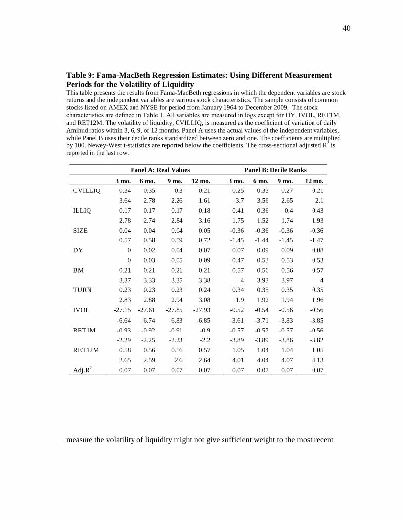
40

40

Table 9: Fama-MacBeth Regression Estimates: Using Different Measurement

Periods for the Volatility of Liquidity This table presents the results from Fama-MacBeth regressions in which the dependent variables are stock

returns and the independent variables are various stock characteristics. The sample consists of common

stocks listed on AMEX and NYSE for period from January 1964 to December 2009. The stock

characteristics are defined in Table 1. All variables are measured in logs except for DY, IVOL, RET1M,

and RET12M. The volatility of liquidity, CVILLIQ, is measured as the coefficient of variation of daily

Amihud ratios within 3, 6, 9, or 12 months. Panel A uses the actual values of the independent variables,

while Panel B uses their decile ranks standardized between zero and one. The coefficients are multiplied

by 100. Newey-West t-statistics are reported below the coefficients. The cross-sectional adjusted R2 is

reported in the last row.

Panel A: Real Values

Panel B: Decile Ranks

3 mo. 6 mo. 9 mo. 12 mo.

3 mo. 6 mo. 9 mo. 12 mo.

CVILLIQ 0.34 0.35 0.3 0.21

0.25 0.33 0.27 0.21

3.64 2.78 2.26 1.61

3.7 3.56 2.65 2.1

ILLIQ 0.17 0.17 0.17 0.18

0.41 0.36 0.4 0.43

2.78 2.74 2.84 3.16

1.75 1.52 1.74 1.93

SIZE 0.04 0.04 0.04 0.05

-0.36 -0.36 -0.36 -0.36

0.57 0.58 0.59 0.72

-1.45 -1.44 -1.45 -1.47

DY 0 0.02 0.04 0.07

0.07 0.09 0.09 0.08

0 0.03 0.05 0.09

0.47 0.53 0.53 0.53

BM 0.21 0.21 0.21 0.21

0.57 0.56 0.56 0.57

3.37 3.33 3.35 3.38

4 3.93 3.97 4

TURN 0.23 0.23 0.23 0.24

0.34 0.35 0.35 0.35

2.83 2.88 2.94 3.08

1.9 1.92 1.94 1.96

IVOL -27.15 -27.61 -27.85 -27.93

-0.52 -0.54 -0.56 -0.56

-6.64 -6.74 -6.83 -6.85

-3.61 -3.71 -3.83 -3.85

RET1M -0.93 -0.92 -0.91 -0.9

-0.57 -0.57 -0.57 -0.56

-2.29 -2.25 -2.23 -2.2

-3.89 -3.89 -3.86 -3.82

RET12M 0.58 0.56 0.56 0.57

1.05 1.04 1.04 1.05

2.65 2.59 2.6 2.64

4.01 4.04 4.07 4.13

Adj.R2 0.07 0.07 0.07 0.07

0.07 0.07 0.07 0.07

measure the volatility of liquidity might not give sufficient weight to the most recent

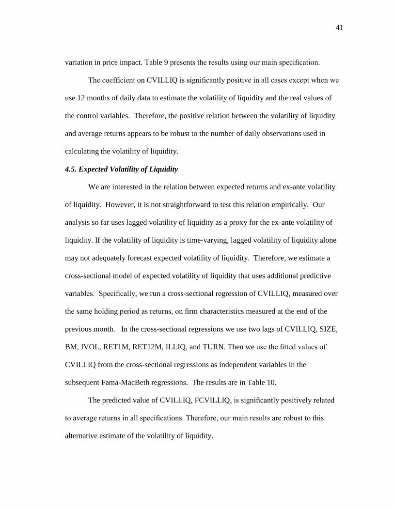
41

41

variation in price impact. Table 9 presents the results using our main specification.

The coefficient on CVILLIQ is significantly positive in all cases except when we

use 12 months of daily data to estimate the volatility of liquidity and the real values of

the control variables. Therefore, the positive relation between the volatility of liquidity

and average returns appears to be robust to the number of daily observations used in

calculating the volatility of liquidity.

4.5. Expected Volatility of Liquidity

We are interested in the relation between expected returns and ex-ante volatility

of liquidity. However, it is not straightforward to test this relation empirically. Our

analysis so far uses lagged volatility of liquidity as a proxy for the ex-ante volatility of

liquidity. If the volatility of liquidity is time-varying, lagged volatility of liquidity alone

may not adequately forecast expected volatility of liquidity. Therefore, we estimate a

cross-sectional model of expected volatility of liquidity that uses additional predictive

variables. Specifically, we run a cross-sectional regression of CVILLIQ, measured over

the same holding period as returns, on firm characteristics measured at the end of the

previous month. In the cross-sectional regressions we use two lags of CVILLIQ, SIZE,

BM, IVOL, RET1M, RET12M, ILLIQ, and TURN. Then we use the fitted values of

CVILLIQ from the cross-sectional regressions as independent variables in the

subsequent Fama-MacBeth regressions. The results are in Table 10.

The predicted value of CVILLIQ, FCVILLIQ, is significantly positively related

to average returns in all specifications. Therefore, our main results are robust to this

alternative estimate of the volatility of liquidity.

42

42

Table 10: Fama-MacBeth Regression Estimates: Using the Predicted Value of the

Volatility of Liquidity This table presents the results from Fama-MacBeth regressions in which the dependent variables are stock returns and the independent variables are various stock characteristics. The sample consists of common stocks listed on AMEX and NYSE for period from January 1964 to December 2009. The stock characteristics are defined in Table 1. The volatility of liquidity is estimated from a cross-sectional model. Specifically, we run a cross-sectional regression of CVILLIQ, measured over the same holding period as returns, on firm characteristics measured at the end of the previous month. In the cross-sectional regressions we use two lags of CVILLIQ, SIZE, BM, IVOL, RET1M, RET12M, ILLIQ, and TURN. Then we use the fitted values of CVILLIQ from the cross-sectional regressions as independent variables in the subsequent Fama-MacBeth regressions. The fitted value is denoted by FCVILLIQ. Panel A uses the actual values of the independent variables, while Panel B uses their decile ranks standardized between zero and one. The coefficients are multiplied by 100. Newey-West t-statistics are reported below the coefficients. The cross-sectional adjusted R

2 is reported in the last row.

Panel A: Real Values

Panel B: Decile Ranks

1 2 3

1 2 3

FCVILLIQ 1.49 1.31 0.89

0.48 0.37 0.33

4.25 3.69 2.67

2.5 1.81 2.19

ILLIQ -0.1 -0.1 0.13

-0.66 -0.5 0.1

-2.5 -1.97 1.86

-2.92 -2.18 0.41

SIZE -0.1 -0.13 0.01

-0.68 -0.62 -0.52

-2.2 -2.1 0.17

-2.68 -2.35 -2.13

DY 0.73 0.67 0

0.24 0.18 0.06

0.83 0.71 0

1.4 1.03 0.4

RET712 0.97

0.96

5.22

5.82

RET46 1.04

0.68

3.58

3.36

RET23 -0.1

-0.24

-0.4

-1.37

1/PRC 0.03 0

0.14

0.28 -0.03

0.68

BM 0.23 0.21 0.2

0.58 0.56

3.59 3.14 3.15

4.12 3.92

TURN

0.22

0.28

2.66

1.66

IVOL

-26.69

-0.49

-6.13

-3.42

RET1M

-1.2 -0.84

0.16 -0.54 -0.53

-3.21 -2.07

0.8 -3.9 -3.68

RET12M

0.62 0.59

0.58 1.11 1.07

2.85 2.71

4.21 4.26 4.15

Adj.R2 0.07 0.06 0.07

0.07 0.06 0.07

43

43

4.6. Additional Robustness Checks

In this section we address some remaining concerns about the main results. We

report our findings which are not tabulated in the dissertation but are available upon

request. First, since our findings are stronger among small stocks, it might be the case

that the findings are driven by the January effect documented by Keim (1983) (see also

Tinic and West (1986), Eleswarapu and Reinganum (1993), and Amihud (2002)). In

separate regressions and sorting analysis we control for the January effect and find

similar results.

Second, the volatility of liquidity measure CVILLIQ might capture an interaction

effect between past returns and trading volume. For example, Cooper (1999) and Lee

and Swaminathan (2001) document that return continuations accentuate with volume,

while Avramov et al. (2006) show that the short term return reversals accentuate with

volume. Accordingly, we include an interaction term between trading volume and past

returns and trading volume and contemporaneous returns in the Fama-MacBeth

regressions. We find that the coefficient on CVILLIQ remains positive and significant.

Third, Acharya and Pederson (2005) argue that a 30% cap should be imposed on

the Amihud ratio measure since anything greater than that due to low volume days might

be unreasonable. We show that our results are not affected by imposing a 30% cap on

the daily components of the liquidity measure.

In addition, Asparouhova et al. (2010) show that microstructure-induced noise in

prices can lead to biases in empirical asset pricing tests. We employ the correction for

this bias suggested by Asparouhova et al. (2010) and we find that the results remain

44

44

robust. Therefore, it is unlikely that our main results are driven by microstructure-

induced noise.

Finally, to ensure that our results are not driven by a non-linear relation between

illiquidity and future returns, we include ILLIQ-squared in the regressions and find

similar results. In additional, return skewness does not seem to influence our main

findings.

45

45

5. THE IDIOSYNCRATIC COMPONENT OF VOLATILITY OF

LIQUIDITY

Our results so far indicate that total volatility of liquidity is positively related to

expected returns. In this section we present a formal approach of extracting the

idiosyncratic component of liquidity risk. Our goal is to examine whether this is the

component that drives the cross-sectional pricing abilities of total volatility of liquidity.

We extract the idiosyncratic volatility of liquidity for each stock i in every month

t using daily data within the month. In particular, we regress daily firm-level illiquidity

on daily excess market returns and daily changes in market illiquidity:

DPIOF= αit +βR

illiq,i,t*ExcessMKTRETd,t + βIilliq,i,t*∆MKTILLIQd,t + ei,d,t (4)

and the measure of idiosyncratic liquidity volatility is:

CVILLIQidios

= SD(ei,d,t)t/ILLIQi,t (5)

The coefficient βR

illiq measures the covariance of stock illiquidity while the

coefficient βIilliq measures the covariance of stock illiquidity with aggregate market

illiquidity. Both of these reflect systematic variations in firm-level illiquidity.

We further estimate systematic variation in stock returns by regressing daily

firm-level excess returns on daily excess market returns and daily changes in market

illiquidity:

Ri,d,t = αit +βR

r,i,t*ExcessMKTRETd,t + βIr,i,t*∆MKTILLIQd,t + ui,d,t (6)

where βR

r,i,t is market betas and βIr,i,t is the covariance of stock return and aggregate

market liquidity.

46

46

The four beta coefficients from equations (4) and (6) are very similar to the

systematic liquidity and return risks examined by Acharya and Pedersen (2005). Our

objective is to test whether idiosyncratic liquidity risk measured by CVILLIQidios

is

priced in the presence of these four betas. Motivated by Acharya and Pedersen (2005),

we additionally control for the covariance between daily stock returns and daily stock

illiquidity over month t, COV(r, illiq). We also control for the skewness of daily returns,

SKEW.

The results are presented in Table 11. The results show that idiosyncratic

liquidity risk CVLLIQidios

is positively and significantly related to expected returns in all

specifications. After controlling for various firm characteristics and risk exposures,

stocks in the highest CVILLIQidios

percentile earn on average 27 basis points per

month more than stocks in the lowest CVILLIQidios

percentile when we use excess

returns as dependent variable. The magnitude is similar when we use risk-adjusted

returns.

Acharya and Pederson (2005) find that the covariance between an asset’s

illiquidity and the market return is significantly negatively related to stock returns. This

is the case since investors are willing to accept a lower expected return for a security that

is less illiquid in a down market. The results in Table 11 are consistent with Acharya and

Pederson (2005). However βR

illiq is significant only when the decile ranks of the

independent variables are used.

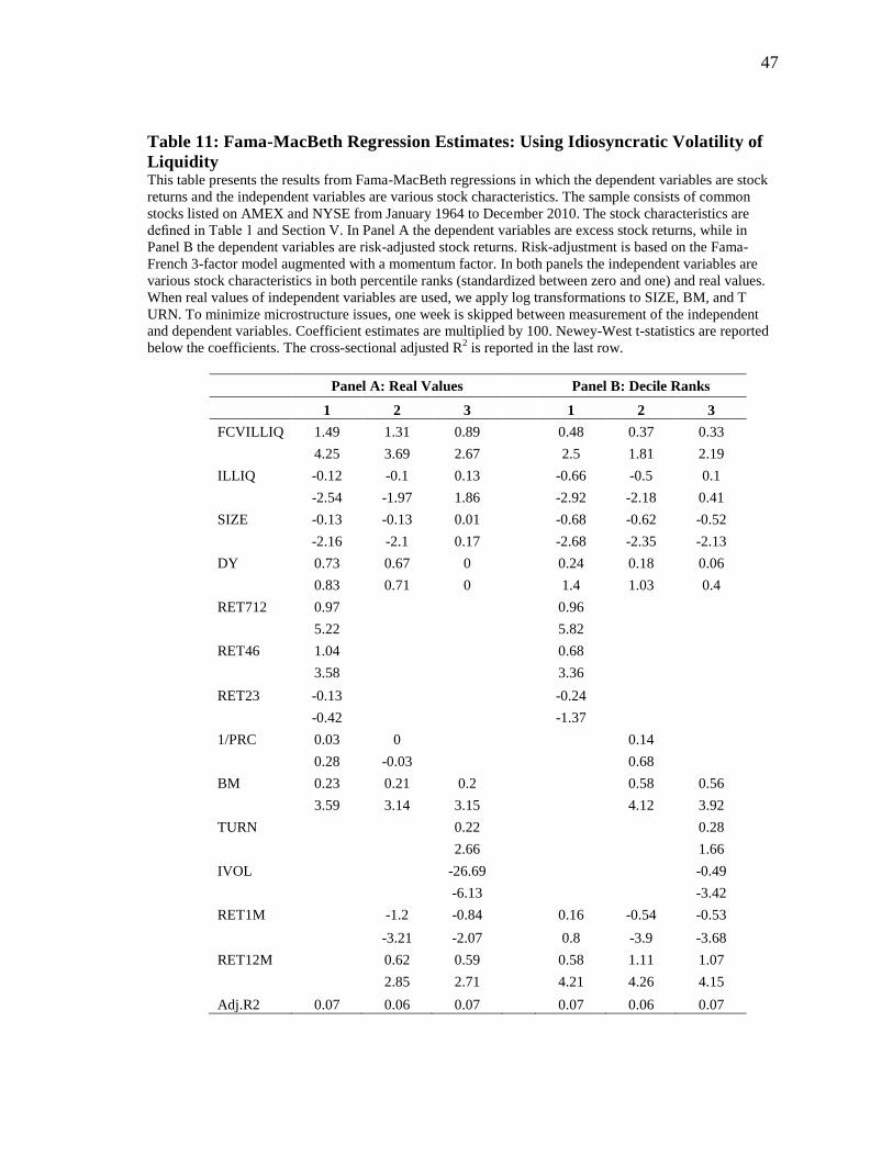
47

47

Table 11: Fama-MacBeth Regression Estimates: Using Idiosyncratic Volatility of

Liquidity This table presents the results from Fama-MacBeth regressions in which the dependent variables are stock

returns and the independent variables are various stock characteristics. The sample consists of common

stocks listed on AMEX and NYSE from January 1964 to December 2010. The stock characteristics are

defined in Table 1 and Section V. In Panel A the dependent variables are excess stock returns, while in

Panel B the dependent variables are risk-adjusted stock returns. Risk-adjustment is based on the Fama-

French 3-factor model augmented with a momentum factor. In both panels the independent variables are

various stock characteristics in both percentile ranks (standardized between zero and one) and real values.

When real values of independent variables are used, we apply log transformations to SIZE, BM, and T

URN. To minimize microstructure issues, one week is skipped between measurement of the independent

and dependent variables. Coefficient estimates are multiplied by 100. Newey-West t-statistics are reported

below the coefficients. The cross-sectional adjusted R2 is reported in the last row.

Panel A: Real Values

Panel B: Decile Ranks

1 2 3

1 2 3

FCVILLIQ 1.49 1.31 0.89

0.48 0.37 0.33

4.25 3.69 2.67

2.5 1.81 2.19

ILLIQ -0.12 -0.1 0.13

-0.66 -0.5 0.1

-2.54 -1.97 1.86

-2.92 -2.18 0.41

SIZE -0.13 -0.13 0.01

-0.68 -0.62 -0.52

-2.16 -2.1 0.17

-2.68 -2.35 -2.13

DY 0.73 0.67 0

0.24 0.18 0.06

0.83 0.71 0

1.4 1.03 0.4

RET712 0.97

0.96

5.22

5.82

RET46 1.04

0.68

3.58

3.36

RET23 -0.13

-0.24

-0.42

-1.37

1/PRC 0.03 0

0.14

0.28 -0.03

0.68

BM 0.23 0.21 0.2

0.58 0.56

3.59 3.14 3.15

4.12 3.92

TURN

0.22

0.28

2.66

1.66

IVOL

-26.69

-0.49

-6.13

-3.42

RET1M

-1.2 -0.84

0.16 -0.54 -0.53

-3.21 -2.07

0.8 -3.9 -3.68

RET12M

0.62 0.59

0.58 1.11 1.07

2.85 2.71

4.21 4.26 4.15

Adj.R2 0.07 0.06 0.07

0.07 0.06 0.07

48

48

A possible explanation behind the insignificant coefficient on βR

illiq when we

use real values of the independent variables could be the presence of considerable

skewness in the cross sectional distribution of βR

illiq. The covariance between an

asset’s return and the market illiquidity, βR

illiq, has a positive and significant

coefficient. The significance fades away when we use real values of the independent

variables which again could be due to extreme outliers. Finally the covariance

between stock illiquidity and market illiquidity is insignificant in any specification.

Overall, the results in Table 11 suggest that idiosyncratic volatility of

liquidity is significantly positively related to average returns. This relation persists

over and above the correlation between systematic liquidity risk and returns.

Therefore, the previously documented relation between total volatility of liquidity

and expected returns is driven by the idiosyncratic component of liquidity volatility.

This result is puzzling in light of Acharya and Pedersen (2005) who document the

pricing of systematic liquidity betas only.

49

49

6. CONCLUSION

In this study we find that the volatility of liquidity is positively related to future

returns. The positive correlation between the volatility of liquidity and expected returns

suggests that risk averse investors require a risk premium for holding stocks that have

high variation in liquidity. Our results are robust to various control variables, systematic

risk factors, and different sub-periods. Higher variation in liquidity implies that a stock

may become illiquid with higher probability at a time when it is traded. This is

important for investors who may face an immediate liquidity need due to exogenous

cash needs, margin calls, dealer inventory rebalancing, or forced liquidations. In case of

such liquidations, the investor may not be able to time the market by waiting for periods

of high liquidity and thus, the level of liquidity on the day of the liquidity need is

important. Overall all our results suggest that besides the mean level of liquidity, the

second moment of liquidity also matters and is significantly related to future returns.

50

50

REFERENCES

Acharya, Viral V., and Lasse Heje Pedersen, 2005, Asset pricing with liquidity risk,

Journal of Financial Economics 77, 375-410.

Amihud, Yakov, 2002, Illiquidity and stock returns: Cross-section and time-series

effects, Journal of Financial Markets 5, 31-56.

Amihud, Yakov, and Haim Mendelson, 1986, Asset pricing and the bid-ask spread,

Journal of Financial Economics 17, 223-249.

Amihud, Yakov, and Haim Mendelson, 1989, The effects of beta, bid-ask spread,

residual risk and size on stock returns, Journal of Finance 44, 479486.

Amihud, Yakov, Haim Mendelson, and Robert A. Wood, 1990, Liquidity and the 1987

stock market crash, Journal of Portfolio Management 16, 65-69.

Ang, Andrew, Robert J. Hodrick, Yuhang Xing, and Xiaoyan Zhang, 2006, The cross-

section of volatility and expected returns, Journal of Finance 61, 259-299.

Atkins, Allen B., and Edward A. Dyl, 1997, Market structure and reported trading

volume: NASDAQ versus the NYSE, Journal of Financial Research 20, 291-304.

Avramov, Doron, Tarun Chordia, and Amit Goyal, 2006, Liquidity and autocorrelations

in individual stock returns, Journal of Finance 61, 2365-2394.

Barinov, Alexander, 2010, Turnover: Liquidity or uncertainty? Working paper,

University of Georgia.

Ben-Raphael, Azi, Ohad Kadan, and Avi Wohl, 2009, The diminishing liquidity

premium, Working paper, Tel Aviv University.

Bertsimas, Dimitris and Andrew W. Lo, 1998, Optimal control of execution costs,

Journal of Financial Markets 1, 1-50.

Blume, Lawrence, David Easley, and Maureen O’Hara, 1994. Market statistics and

technical analysis: The role of volume, Journal of Finance 49, 153-181.

Brennan, Michael J., Tarun Chordia and Avanidhar Subrahmanyam, 1998, Alternative

factor specifications, security characteristics, and the cross-section of expected stock

returns, Journal of Financial Economics 49, 345-373.

51

51

Brennan, Michael J., and Avanidhar Subrahmanyam, 1996, Market microstructure and

asset pricing: On the compensation for illiquidity in stock returns, Journal of

Financial Economics 41, 441-464.

Brunnermeier, Markus, and Lasse Pedersen, 2009, Market liquidity and funding

liquidity, Review of Financial Studies 22, 22012238.

Chalmers, John R., and Gregor Kadlec, (1998), An empirical examination of the

amortized spread, Journal of Financial Economics 48, 159-188.

Chan, Louis K., and John Lakonishok, 1995, The behavior of stock prices around

institutional trades, Journal of Finance 50, 1147-1174.

Chen, Hsiu-Lang, Narasimhan Jegadeesh, and Russ Wermers, 2000, The value of active

mutual fund management: An examination of the stock holdings and trades of fund

managers, Journal of Financial and Quantitative Analysis 35, 343-368.

Chordia, Tarun, Richard Roll, and Avanidhar Subrahmanyam, 2001, Market liquidity

and trading activity, Journal of Finance 56, 501-530.

Chordia, Tarun, Huh Sahn-Wook, and Avanidhar Subrahmanyam, 2009, Theory-Based

illiquidity and asset pricing, Review of Financial Studies 22, 3629-3668.

Chordia, Tarun, Avanidhar Subrahmanyam, and V. Ravi Anshuman, 2001, Trading

activity and expected stock returns, Journal of Financial Economics 59, 3-32.

Cooper, Michael, 1999, Filter rules based on price and volume in individual security

overreaction, Review of Financial Studies 12, 901-935.

Dimson, Elroy, 1979, Risk measurement when shares are subject to infrequent trading,

Journal of Financial Economics 7, 197-226.

Eleswarapu, Venkat R., 1997, Cost of transacting and expected returns in the NASDAQ

Market, Journal of Finance 52, 2113-2127.

Eleswarapu, Venkat, and M. Reinganum, 1993, The seasonal behavior of liquidity

premium in asset pricing, Journal of Financial Economics 34, 373-386.

Fama, Eugene F., and Kenneth R. French, 1993, Common risk factors in the returns on

stocks and bonds, Journal of Financial Economics 33, 3-56.

Fama, Eugene F., and Kenneth R. French, 2002, Testing trade-off and pecking order

predictions about dividends and debt, Review of Financial Studies 15, 1-33.

Fama, Eugene F. and James D. MacBeth, 1973, Risk, return, and equilibrium: Empirical

tests, Journal of Political Economy 81, 607-636.

52

52

Garleanu, Nicolae, and Lasse Heje Pedersen, 2007, Liquidity and risk management,

American Economic Review 97, 193197.

Gervais, Simon, Ron Kaniel, and Daniel Mingelgrin, 2001, The high-volume return

premium, Journal of Finance 56, 877-919.

Goyenko, RuslanY., Craig W. Holden, and Charles A. Trzcinka, 2009, Do liquidity

measures measure liquidity? Journal of Financial Economics 92, 153-181.

Gromb, Denis, and Dimitri Vayanos, 2002, Equilibrium and welfare in markets with

financially constrained arbitrageurs, Journal of Financial Economics 66, 361407.

Harris, Milton, and Artur Raviv, 1993, Differences of opinion make a horse race, Review

of Financial Studies 6, 473-506.

Hasbrouck, Joel, 2009, Trading costs and returns for U.S. equities: Estimating effective

costs from daily data, Journal of Finance 64, 1445-1477.

Hasbrouck, Joel, and Duane J. Seppi, 2001, Common factors in prices, order flows, and

liquidity, Journal of Financial Economics 59, 383411.

He, Hua., and Harry Mamayasky, 2005, Dynamic trading policies with price impact,

Journal of Economic Dynamics and Control 29, 891-930.

Huang, Ming, 2003, Liquidity shocks and equilibrium liquidity premia, Journal of

Economic Theory 109, 104-129.

Jegadeesh, Narasimhan, 1990, Evidence of predictable behavior of security returns,

Journal of Finance 45, 881-898.

Jegadeesh, Narasimhan, and Sheridan Titman, 1993, Returns to buying winners and

selling losers: Implications for stock market efficiency, Journal of Finance 48, 65-

91.

Karpoff, Jonathan M., 1986, A theory of trading volume, Journal of Finance 41, 1069-

1087.

Keim, Donald B., 1983, Size-related anomalies and stock return seasonality, Journal of

Financial Economics 12, 13-32.

Keim, Donald B., and Ananth Madhavan, 1996, The upstairs market for large-block

transactions: Analysis and measurement of price effects, Review of Financial

Studies 9, 1-36.

53

53

Korajczyk, Robert A., and Ronnie Sadka, 2008, Pricing the commonality across

alternative measures of liquidity, Journal of Financial Economics 87, 45-72.

Koren, Miklos, and Adam Szeidl, 2002, Portfolio choice with illiquid assets, Working

paper, Harvard University.

Kyle, Albert S., 1985, Continuous auctions and insider trading, Econometrica 53, 1315-

1335.

Lee, Charles M. C., and Bhaskaran Swaminathan, 2000, Price momentum and trading

volume, Journal of Finance 55, 2017-2069.

Lowenstein, Roger, 2000, When genius failed: The rise and fall of Long-Term Capital

Management (Random House, New York).

Merton, Robert C., 1987, A simple model of capital market equilibrium with incomplete

information, Journal of Finance 42, 483-510.

Miller, Edward M., 1977, Risk, uncertainty, and divergence of opinion, Journal of

Finance 32, 1151-1168.

Morris, Stephen, and Hyun Song Shin, 2004, Liquidity black holes, Review of Finance 8,

118.

Nagel, Stefan, 2005, Short sales, institutional investors and the cross-section of stock

returns, Journal of Financial Economics 78, 277-309.

Pastor, Lubos, and Robert F. Stambaugh, 2003, Liquidity risk and expected stock returns,

Journal of Political Economy 111, 642-685.

Pereira, Joo P., and Harold H. Zhang, 2011, Stock returns and the volatility of liquidity,

Journal of Financial and Quantitative Analysis, Forthcoming.

Roll, Richard, and Avanidhar Subrahmanyam, 2009, Liquidity skewness, Working

paper, University of California, Los Angeles.

Sadka, Ronnie, 2006, Momentum and post-earnings announcement drift anomalies: The

role of liquidity risk, Journal of Financial Economics 80, 309-349.

Spiegel, Matthew I., and Xiaotong Wang, 2005, Cross-sectional variation in stock

returns: Liquidity and idiosyncratic risk, Working Paper, Yale University.

Tinic, Seha M., and Richard R. West, 1986, Risk, return and equilibrium: A revisit,

Journal of Political Economy 94, 126-147.

54

54

Vayanos, Dimitri, 2004, Flight to quality, flight to liquidity and the pricing of risk,

National Bureau of Economic Research working paper.

Yan, X. and Zhang, Z, 2009, Institutional investors and equity returns: Are short term

institutions better informed? Review of Financial Studies 22, 893-924.

55

55

VITA

Name: Ferhat Akbas

Address: Department of Finance

Mays Business School

Texas A&M University

4353 TAMU

College Station, TX 77843-4353

Email Address: ferhat_akbas@hotmail.com

Education: B.S., Industrial Engineering, Bilkent University, 2003

M.S., Economics, Texas A&M University, 2007

Ph.D., Finance, Texas A&M University, 2011

Awards: Texas A&M University, Graduate Studies Scholarship, 2004 – 2011

Mays Business School Fellowship, 2007-2011