liquidity risk and expected stock...
TRANSCRIPT
642
[Journal of Political Economy, 2003, vol. 111, no. 3]� 2003 by The University of Chicago. All rights reserved. 0022-3808/2003/11103-0006$10.00
Liquidity Risk and Expected Stock Returns
Lubos PastorUniversity of Chicago, National Bureau of Economic Research, and Centre for Economic PolicyResearch
Robert F. StambaughUniversity of Pennsylvania and National Bureau of Economic Research
This study investigates whether marketwide liquidity is a state variableimportant for asset pricing. We find that expected stock returns arerelated cross-sectionally to the sensitivities of returns to fluctuationsin aggregate liquidity. Our monthly liquidity measure, an average ofindividual-stock measures estimated with daily data, relies on the prin-ciple that order flow induces greater return reversals when liquidityis lower. From 1966 through 1999, the average return on stocks withhigh sensitivities to liquidity exceeds that for stocks with low sensitiv-ities by 7.5 percent annually, adjusted for exposures to the marketreturn as well as size, value, and momentum factors. Furthermore, aliquidity risk factor accounts for half of the profits to a momentumstrategy over the same 34-year period.
Research support from the Center for Research in Security Prices and the James S.Kemper Faculty Research Fund at the Graduate School of Business, University of Chicago,is gratefully acknowledged (Pastor). We are grateful for comments from Nick Barberis,John Campbell, Tarun Chordia, John Cochrane (the editor), George Constantinides, DougDiamond, Andrea Eisfeldt, Gene Fama, Simon Gervais, David Goldreich, Gur Huberman,Michael Johannes, Owen Lamont, Andrew Metrick, Mark Ready, Hans Stoll, Dick Thaler,Rob Vishny, Tuomo Vuolteenaho, Jiang Wang, and two anonymous referees, as well asworkshop participants at Columbia University, Harvard University, New York University,Stanford University, University of Arizona, University of California at Berkeley, Universityof Chicago, University of Florida, University of Pennsylvania, Washington University, theReview of Financial Studies Conference on Investments in Imperfect Capital Markets atNorthwestern University, the Fall 2001 NBER Asset Pricing meeting, and the 2002 WesternFinance Association meetings.
liquidity risk 643
I. Introduction
In standard asset pricing theory, expected stock returns are related cross-sectionally to returns’ sensitivities to state variables with pervasive effectson investors’ overall welfare. A security whose lowest returns tend toaccompany unfavorable shifts in that welfare must offer additional com-pensation to investors for holding the security. Liquidity appears to bea good candidate for a priced state variable. It is often viewed as animportant feature of the investment environment and macroeconomy,and recent studies find that fluctuations in various measures of liquidityare correlated across assets.1 This empirical study investigates whethermarketwide liquidity is indeed priced. That is, we ask whether cross-sectional differences in expected stock returns are related to the sen-sitivities of returns to fluctuations in aggregate liquidity.
It seems reasonable that many investors might require higher ex-pected returns on assets whose returns have higher sensitivities to ag-gregate liquidity. Consider, for example, any investor who employs someform of leverage and faces a margin or solvency constraint, in that ifhis overall wealth drops sufficiently, he must liquidate some assets toraise cash. If he holds assets with higher sensitivities to liquidity, thensuch liquidations are more likely to occur when liquidity is low, sincedrops in his overall wealth are then more likely to accompany drops inliquidity. Liquidation is costlier when liquidity is lower, and those greatercosts are especially unwelcome to an investor whose wealth has alreadydropped and who thus has higher marginal utility of wealth. Unless theinvestor expects higher returns from holding these assets, he wouldprefer assets less likely to require liquidation when liquidity is low, evenif these assets are just as likely to require liquidation on average.2
The well-known 1998 episode involving Long-Term Capital Manage-ment (LTCM) seems an acute example of the liquidation scenario above.
1 Chordia, Roll, and Subrahmanyam (2000), Lo and Wang (2000), Hasbrouck and Seppi(2001), and Huberman and Halka (2002) empirically analyze the systematic nature ofstock market liquidity. Chordia, Sarkar, and Subrahmanyam (2002) find that improvementsin stock market liquidity are associated with monetary expansions and that fluctuationsin liquidity are correlated across stocks and bond markets. Eisfeldt (2002) develops amodel in which endogenous fluctuations in liquidity are correlated with real fundamentalssuch as productivity and investment.
2 This economic story has yet to be formally modeled, but recent literature presentsrelated models that lead to the same basic result. Lustig (2001) develops a model in whichsolvency constraints give rise to a liquidity risk factor, in addition to aggregate consumptionrisk, and equity’s sensitivity to the liquidity factor raises its equilibrium expected return.Holmstrom and Tirole (2001) also develop a model in which a security’s expected returnis related to its covariance with aggregate liquidity. Unlike more standard models, theirmodel assumes risk-neutral consumers and is driven by liquidity demands at the corporatelevel. Acharya and Pedersen (2002) develop a model in which each asset’s return is netof a stochastic liquidity cost, and expected returns are related to return covariances withthe aggregate liquidity cost (as well as to three other covariances).
644 journal of political economy
The hedge fund was highly levered and by design had positive sensitivityto marketwide liquidity, in that many of the fund’s spread positions,established across a variety of countries and markets, went long lessliquid instruments and short more liquid instruments. When the Russiandebt crisis precipitated a widespread deterioration in liquidity, LTCM’sliquidity-sensitive portfolio dropped sharply in value, triggering a needto liquidate in order to meet margin calls. The anticipation of costlyliquidation in a low-liquidity environment then further eroded LTCM’sposition. (The liquidation was eventually overseen by a consortium of14 institutions organized by the New York Federal Reserve.) Even thoughexposure to liquidity risk ultimately spelled LTCM’s doom, the fundperformed quite well in the previous four years, and presumably itsmanagers perceived high expected returns on its liquidity-sensitivepositions.3
Liquidity is a broad and elusive concept that generally denotes theability to trade large quantities quickly, at low cost, and without movingthe price. We focus on an aspect of liquidity associated with temporaryprice fluctuations induced by order flow. Our monthly aggregate li-quidity measure is a cross-sectional average of individual-stock liquiditymeasures. Each stock’s liquidity in a given month, estimated using thatstock’s within-month daily returns and volume, represents the averageeffect that a given volume on day d has on the return for day d � 1,when the volume is given the same sign as the return on day d. Thebasic idea is that, if signed volume is viewed roughly as “order flow,”then lower liquidity is reflected in a greater tendency for order flow ina given direction on day d to be followed by a price change in theopposite direction on day Essentially, lower liquidity correspondsd � 1.to stronger volume-related return reversals, and in this respect our li-quidity measure follows the same line of reasoning as the model andempirical evidence presented by Campbell, Grossman, and Wang(1993). They find that returns accompanied by high volume tend to bereversed more strongly, and they explain how this result is consistentwith a model in which some investors are compensated for accommo-dating the liquidity demands of others.
We find that stocks’ “liquidity betas,” their sensitivities to innovationsin aggregate liquidity, play a significant role in asset pricing. Stocks withhigher liquidity betas exhibit higher expected returns. In particular,between January 1966 and December 1999, a spread between the topand bottom deciles of predicted liquidity betas produces an abnormalreturn (“alpha”) of 7.5 percent per year with respect to a model thataccounts for sensitivities to four other factors: the market, size, and valuefactors of Fama and French (1993) and a momentum factor. The alpha
3 See, e.g., Jorion (2000) and Lowenstein (2000) for accounts of the LTCM experience.

liquidity risk 645
with respect to just the three Fama-French factors is over 9 percent peryear. The results are both statistically and economically significant, andsimilar results occur in both halves of the overall 34-year period.
This study investigates whether expected returns are related to sys-tematic liquidity risk in returns, as opposed to the level of liquidity perse. The latter’s relation to expected stock returns has been investigatedby numerous empirical studies, including Amihud and Mendelson(1986), Brennan and Subrahmanyam (1996), Brennan, Chordia, andSubrahmanyam (1998), Datar, Naik, and Radcliffe (1998), and Fiori(2000).4 Using a variety of liquidity measures, these studies generallyfind that less liquid stocks have higher average returns. Amihud (2002)and Jones (2002) document the presence of a time-series relation be-tween their measures of market liquidity and expected market returns.Instead of investigating the level of liquidity as a characteristic that isrelevant for pricing, this study entertains marketwide liquidity as a statevariable that affects expected stock returns because its innovations haveeffects that are pervasive across common stocks. The potential usefulnessof such a perspective is recognized by Chordia, Roll, and Subrahmanyam(2000, 2001).
Chordia, Subrahmanyam, and Anshuman (2001) find a significantcross-sectional relation between stock returns and the variability of li-quidity, where liquidity is proxied by measures of trading activity suchas volume and turnover. The authors report that stocks with more vol-atile liquidity have lower expected returns, an unexpected result. Li-quidity risk in that study is measured as firm-specific variability in li-quidity. Our paper focuses on systematic liquidity risk in returns andfinds that stocks whose returns are more exposed to marketwide liquidityfluctuations command higher expected returns.
Section II explains the construction of the liquidity measure andbriefly describes some of its empirical features. The sharpest troughs inmarketwide liquidity occur in months easily identified with significantfinancial and economic events, such as the 1987 crash, the beginningof the 1973 oil embargo, the 1997 Asian financial crisis, and the 1998collapse of LTCM. Moreover, in months of large liquidity drops, stockreturns are negatively correlated with fixed-income returns, in contrastto other months. This observation seems consistent with “flight-to-quality” effects. We also find significant commonality across stocks inour monthly liquidity measure. That result, in accord with the high-frequency evidence of previous studies, enhances the prospect that mar-ketwide liquidity could be a priced state variable.
4 Theoretical studies that investigate the relation between liquidity and asset prices in-clude Amihud and Mendelson (1986), Constantinides (1986), Heaton and Lucas (1996),Vayanos (1998), Lo, Mamaysky, and Wang (2001), and Huang (in press), among others.
646 journal of political economy
Section III presents the asset pricing investigation. We find that stocks’liquidity betas can be predicted not only by their simple historical es-timates but by other variables as well. Each year, we sort stocks by theirpredicted liquidity betas and form 10 portfolios. This procedure yieldsa substantial spread in the estimated postformation liquidity betas aswell as the large spread in abnormal returns reported above. Sortingstocks on their historical liquidity betas alone produces results that areslightly less strong but still significant. A sort on firm size reveals thatstocks of the smallest firms tend to have high liquidity betas as well assignificantly positive alphas with respect to the four-factor model.
Section IV provides an investment perspective on liquidity risk byexamining the degree to which spreads between stocks with high andlow liquidity risk expand the mean-variance opportunity set. In an in-vestment universe that also includes the market portfolio and spreadsbased on size, value, and momentum, we find that liquidity risk spreadsreceive substantial weight in the portfolio with the highest ex postSharpe ratio. The importance of the momentum spread in that portfoliois especially reduced as compared to a universe without a liquidity riskspread. Moreover, an equally weighted liquidity risk spread reduces mo-mentum’s alpha by half in the overall 34-year period and eliminates itcompletely (driving it to a small negative value) in the more recent 17-year subperiod 1983–99. Section V briefly reviews our conclusions andsuggests directions for future research.
II. Marketwide Liquidity
A. Constructing a Measure
Liquidity has many dimensions. This study focuses on a dimension as-sociated with temporary price changes accompanying order flow. Weconstruct a measure of market liquidity in a given month as the equallyweighted average of the liquidity measures of individual stocks on theNew York Stock Exchange (NYSE) and American Stock Exchange(AMEX), using daily data within the month.5 Specifically, the liquidity
5 All the individual-stock return and volume data used in the study are obtained fromthe Center for Research in Security Prices (CRSP) at the University of Chicago. Dailyreturns and volume are taken from the CRSP daily stock file; all month-end (or year-end)codes and values are taken from the CRSP monthly stock file. We exclude NASDAQ inconstructing the aggregate liquidity measure because NASDAQ returns and volume dataare available from CRSP for only part of this period (beginning in 1982). Also, reportedvolumes on NASDAQ include interdealer trades, unlike the volumes reported on theNYSE and the AMEX. To exclude NASDAQ, we omit stocks with exchange codes of 3 or33 as of the end of the previous year. We use only stocks classified as ordinary commonshares (CRSP share codes 10 and 11), excluding American depository receipts, shares ofbeneficial interest, certificates, units, real estate investment trusts, closed-end funds, com-panies incorporated outside the United States, and Americus trust components.
liquidity risk 647
measure for stock i in month t is the ordinary least squares estimate ofin the regressiongi,t
e er p v � f r � g sign(r ) 7 v � e , d p 1, … , D, (1)i,d�1,t i,t i,t i,d,t i,t i,d,t i,d,t i,d�1,t
where quantities are defined as follows: is the return on stock i onri,d,t
day d in month t; where is the return on the CRSPer p r � r , ri,d,t i,d,t m,d,t m,d,t
value-weighted market return on day d in month t; and is the dollarvi,d,t
volume for stock i on day d in month t. A stock’s liquidity is computedin a given month only if there are more than 15 observations with whichto estimate the regression (1) ( ), and we exclude a stock for theD 1 15first and last partial month that it appears on the CRSP tape. The dailyobservations are not required to be consecutive (except that each ob-servation requires data for two successive days). Stocks with share pricesless than $5 and greater than $1,000 at the end of the previous monthare excluded, and volume is measured in millions of dollars.
The basic idea is that “order flow,” constructed here simply as volumesigned by the contemporaneous return on the stock in excess of themarket, should be accompanied by a return that one expects to bepartially reversed in the future if the stock is not perfectly liquid. Weassume that the greater the expected reversal for a given dollar volume,the lower the stock’s liquidity. That is, one would expect to be negativegi,t
in general and larger in absolute magnitude when liquidity is lower.6
Viewing volume-related return reversals as arising from liquidity effectsis motivated by Campbell et al. (1993). Those authors present a modelin which risk-averse “market makers,” defined in the general sense ofGrossman and Miller (1988), accommodate order flow from liquidity-motivated traders and are compensated with a higher expected return(by buying at a low price or selling at a high one). The greater theorder flow, the greater the compensation, so this liquidity-induced effecton expected future return is larger when current volume is high. Camp-bell et al. present empirical evidence consistent with this argument.
As illustrated below, the estimates of the liquidity measure aregi,t
typically negative, although there are months in which the average es-timate is positive. The preponderance of negative values is consistentwith the basic intuition underlying our liquidity measure, but it mustbe recognized that the measure abstracts from other potential roles thatvolume can play in the relation between current and lagged return. Forexample, Llorente et al. (2001) explain that asymmetric information(not considered by Campbell et al. [1993]) can weaken the volume-
6 An alternative class of liquidity measures is based on a positive contemporaneous relationbetween returns and order flow. Typically, these measures are estimated with intradaytransactions data, and the volume for a transaction is signed by comparing the transactionprice to the bid-ask midpoint (see, e.g., Hasbrouck 1991; Foster and Viswanathan 1993;Brennan and Subrahmanyam 1996).
648 journal of political economy
related reversal effect and even produce volume-related continuationsin returns on stocks for which information-motivated trading is suffi-ciently important. Using daily data, the authors report empirical evi-dence consistent with that prediction. Other related evidence is reportedby Lee and Swaminathan (2000), who conclude that momentum effectsin monthly returns are stronger for stocks with high recent volume.
The specification of the regression in (1) is somewhat arbitrary, as isany liquidity measure. We use the return in excess of the market,er ,i,d,t
as the dependent variable as well as to sign volume, in order to removemarketwide shocks and better isolate the individual-stock effect of vol-ume-related return reversals. Moreover, daily returns of zero are notuncommon with lower-priced stocks for which a one-tick move repre-sents a greater relative price change. Signing volume on the basis oftotal return is problematic in those zero-return cases, whereas returnsin excess of the market are unlikely to be zero. On a day in which astock’s price does not change but the market goes up, it seems reason-able to identify the stock’s order flow on that day as more likely initiatedby sellers than by buyers. We also include the lagged stock return as asecond independent variable with the intention of capturing lagged-return effects that are not volume-related, such as reversals due to aminimum tick size. Since we use to sign volume, we use the totaleri,d,t
return as this second variable to have it be less correlated with theri,d,t
variable whose coefficient we take as the liquidity measure. (A highercorrelation between the independent variables generally reduces theprecision with which one can measure the individual slope on eitherone.) The precise specification of the variables in (1), as compared toseemingly close alternative specifications, is addressed below in subsec-tion C.
In order to investigate the ability of the regression slope in (1) togi,t
capture a liquidity effect, we examine a simple model in which the returnon a given day has an order flow component that is partially reversedon the subsequent day. Specifically, the return on stock i on day d isgiven by
r p f � u � f(q � q ) � h � h . (2)i,d d i,d i i,d�1 i,d i,d i,d�1
The first two terms on the right-hand side represent permanent changesin the price, where is a marketwide factor and is a stock-specificf ud i,d
effect. The term is intended to capture the liquidity-relatedf(q � q )i i,d�1 i,d
effect arising from order flow in the sense that both current andq ,i,d
lagged order flow enter the return, but in the opposite directions. Thecoefficient fi is negative and represents the stock’s liquidity. We assumethat where is independent across stocks and qd is a∗ ∗q p q � q , qi,d i,d d i,d
marketwide component whose standard deviation is one-third as largeas that of so the marketwide component then explains 10 percent∗q ,i,d
liquidity risk 649
of the total variance of order flow. (Hasbrouck and Seppi [2001] reportthat the first principal component explains 7.8 percent of total orderflow variance.)
We use (2) to simulate returns on 10,000 stocks. The quantities fd,and qd are all mean zero draws from normal distributions. The∗u , q ,i,d i,d
values of fd are drawn independently across d with standard deviation; and are drawn independently across d and i with∗j p 0.20/250 u qi,d i,d
standard deviations equal to j; and qd is drawn independently across dwith standard deviation equal to The liquidity coefficient fi is drawn1
j.3independently across i from a uniform [�1, 0] distribution. The term
represents an additional reversal effect that is independenth � hi,d i,d�1
of the order flow effect, and this component of the return is best viewedas bid-ask bounce or a tick size effect. On a given day, takes the valuehi,d
�si, zero, or si with probabilities one-fourth, one-half, and one-fourth,and the realizations are independent across days and stocks. The valueof si for a given stock is drawn as where is a uniform0.01(U � f), U[0,1] i [0,1]
[0, 1] variate, so the mean value of si across stocks is 0.01, and there issome association between the typical magnitude of and the stock’shi,d
liquidity (less liquid stocks tend to have larger si’s). In this simulationsetting, the average standard deviation of a daily stock return is 0.023,the average standard deviation of each of the first three right-hand-sideterms in (2) is 0.013, and the average standard deviation of h �i,d
is 0.010. The regression in (1) requires returns in excess of thehi,d�1
market, so we also construct a market return as
n1r p r ,�m,d i,dn ip1
for (The average in a regression of on is .33.) We2n p 10,000. R r ri,d m,d
also specify a stock’s “volume” on day d as 7 For each stock,v p Fq F.i,d i,d
we then compute the population value of the coefficient in (1) bygi
estimating that regression across 50,000 simulated daily values. We findthat the cross-sectional correlation between fi and is .98, which sug-gi
gests that the regression in (1) is a reasonable specification for esti-mating the hypothesized liquidity effect.
The use of signed volume as a predictor of future return can also bemotivated using the equilibrium model of Campbell et al. (1993). Intheir model, the stock’s excess return and order flow Dt are jointlyQ t
normal, along with and the regression relating expected futureQ ,t�1
7 Because of the common factor in order flow, the market return is correlated withlagged order flow. Moreover, if we compute a lagged aggregate “volume” measure as
then the correlation between and is �.03. This feature of ourV p � Fq F, r r Vd i,d m,d m,d�1 di
simulation is consistent with the negative relation between the market return and thelagged product of return and volume reported by Campbell et al. (1993).
650 journal of political economy
return to current return and volume Vt ( ) is given by a relationp FDFtof the form
E(Q FQ , V) p f Q � f tanh (f VQ )V, (3)t�1 t t 1 t 2 3 t t t
where and As the correlation between and Dt increases,f ! 0 f ! 0. Q2 3 t
(3) becomes well approximated by
E(Q FQ , V) p f Q � f sign(Q )V, (4)t�1 t t 1 t 2 t t
which is roughly analogous to (1).8 To the extent that order flow playsan important role in determining high-frequency return variation, aconjecture that seems plausible, we see that the model of Campbell etal. gives some justification for the use of signed volume. Of course, theirmodel of a single-stock economy with continuous price variables (nominimum tick) is only suggestive when applied to our empirical setting,but the intuition underlying their model corresponds to our interpre-tation of as a liquidity measure.gi,t
Although the ordinary least squares slope coefficient is an impre-gi,t
cise estimate of a given stock’s the marketwide average liquidity ing ,i,t
month t is estimated more precisely. The disturbances in (1) are lessthan perfectly correlated across stocks (recall that the dependent var-iable is the return in excess of the market). Thus, as the number ofstocks, N, grows large, the true unobserved average N
g p (1/N )� gt i,tip1
becomes more precisely estimated byN1
ˆ ˆg p g . (5)�t i,tN ip1
We construct the marketwide measure above for each month from Au-gust 1962 through December 1999. The number of stocks in the index(N) ranges from 951 to 2,188.
Given the regression specification in (1), the value of can be viewedgi,t
as the liquidity “cost,” in terms of return reversal, of “trading” $1 millionof stock i, so the average in (5) can be viewed as the cost of a $1 milliontrade distributed equally across stocks. Obviously, a dollar trade size of
8 Equation (3) relies on a result given in Wang (1994). It is straightforward to show thatWang’s eq. B.6 allows (3) to be restated as
r Q Vt tE(Q FQ , V ) p f Q � f tanh V ,t�1 t t 1 t 2 t( ) ( ) ( )2[ ]1 � r j jQ D
where r is the correlation between and Dt, and and are the standard deviationsQ j jt Q D
of those variables. Note that as r r 1,
r Q Vt ttanh ( ) ( ) ( )2[ ]1 � r j jQ D
converges in distribution to since and (�1) as (��).sign(Q ) V ≥ 0 tanh (x) r 1 x r �t t
liquidity risk 651
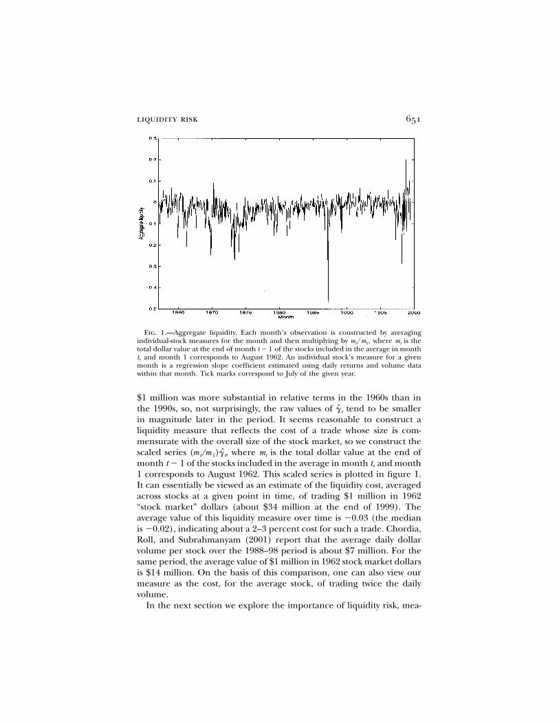
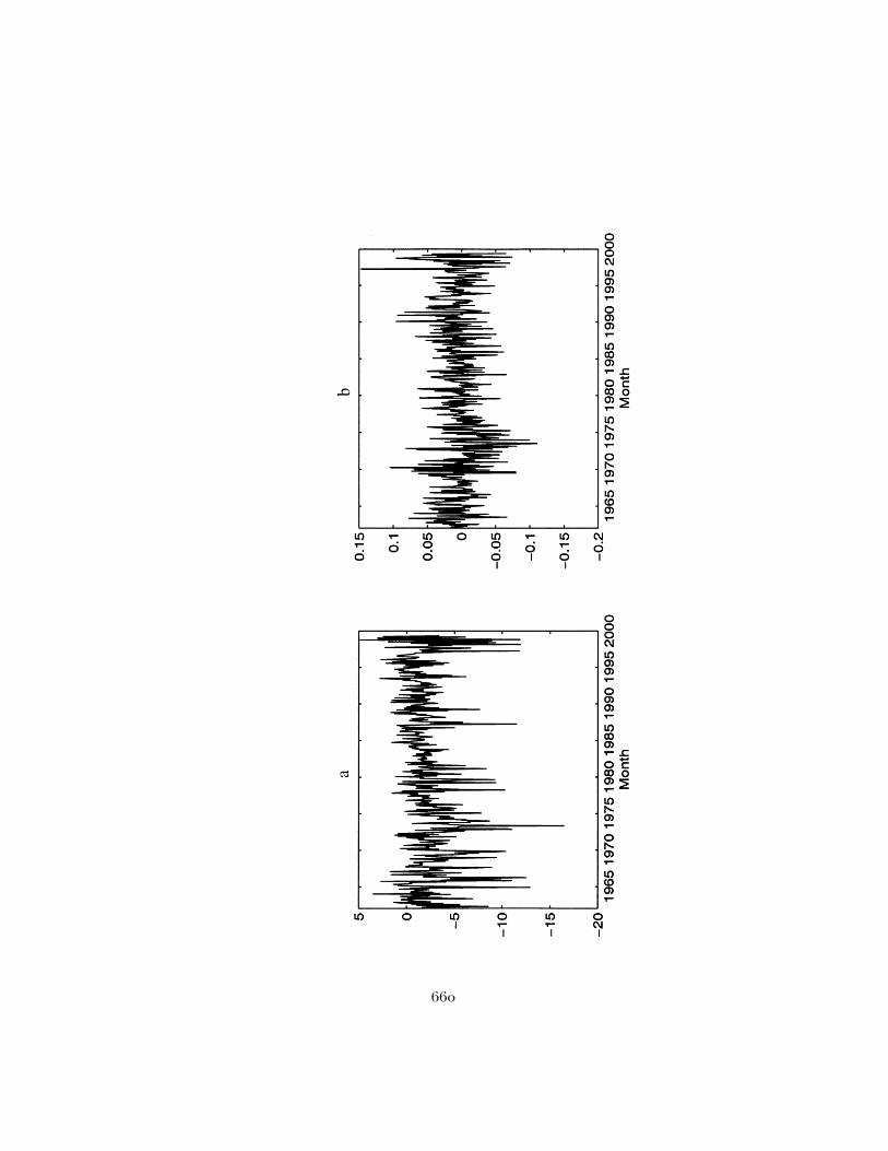
Fig. 1.—Aggregate liquidity. Each month’s observation is constructed by averagingindividual-stock measures for the month and then multiplying by where mt is them /m ,t 1
total dollar value at the end of month of the stocks included in the average in montht � 1t, and month 1 corresponds to August 1962. An individual stock’s measure for a givenmonth is a regression slope coefficient estimated using daily returns and volume datawithin that month. Tick marks correspond to July of the given year.
$1 million was more substantial in relative terms in the 1960s than inthe 1990s, so, not surprisingly, the raw values of tend to be smallergt
in magnitude later in the period. It seems reasonable to construct aliquidity measure that reflects the cost of a trade whose size is com-mensurate with the overall size of the stock market, so we construct thescaled series where mt is the total dollar value at the end ofˆ(m /m )g ,t 1 t
month of the stocks included in the average in month t, and montht � 11 corresponds to August 1962. This scaled series is plotted in figure 1.It can essentially be viewed as an estimate of the liquidity cost, averagedacross stocks at a given point in time, of trading $1 million in 1962“stock market” dollars (about $34 million at the end of 1999). Theaverage value of this liquidity measure over time is �0.03 (the medianis �0.02), indicating about a 2–3 percent cost for such a trade. Chordia,Roll, and Subrahmanyam (2001) report that the average daily dollarvolume per stock over the 1988–98 period is about $7 million. For thesame period, the average value of $1 million in 1962 stock market dollarsis $14 million. On the basis of this comparison, one can also view ourmeasure as the cost, for the average stock, of trading twice the dailyvolume.
In the next section we explore the importance of liquidity risk, mea-
652 journal of political economy
sured as comovement between returns and unanticipated innovationsin liquidity. The liquidity series plotted in figure 1 has a first-order serialcorrelation of .22. In constructing innovations, we do not work directlywith that series, since to do so could introduce a return componentthrough fluctuations in the scaling factor Although any such(m /m ).t 1
return effects would be lagged, since mt uses values at the end of monthwe nevertheless wish to minimize the possibility that any estimatedt � 1,
relation between returns and liquidity innovations could arise in thatfashion. At the same time, the innovation series should also appropri-ately reflect the growth in size of the stock market. Therefore, ratherthan difference the scaled series, we first difference and then scale.Specifically, to construct innovations in liquidity, we first scale themonthly difference in liquidity measures, averaged across the Nt stockswith available data in both the current and previous month,
Ntm 1tˆ ˆ ˆDg p (g � g ). (6)�t i,t i,t�1( )m N ip11 t
We then regress on its lag as well as the lagged value of the scaledˆDgt
level series:
mt�1ˆ ˆ ˆDg p a � bDg � c g � u . (7)t t�1 t�1 t( )m 1
This regression allows the predicted change to depend on the mostrecent change as well as on the deviation of the most recent level fromits long-run mean (impounded in a). Aside from the scaling issues, theregression is analogous to a second-order autoregression in the levelseries, and it produces residuals that appear serially uncorrelated.9 Theinnovation in liquidity, is taken as the fitted residual divided by 100:L ,t
1ˆL p u . (8)t t100
The arbitrary scaling by 100 simply produces more convenient magni-tudes of the liquidity betas reported in the next section. If expectedchanges in liquidity are correlated with time variation in expected stockreturns, then failure to use liquidity innovations can contaminate riskmeasures. We find that expected liquidity changes can indeed predict
9 Note that the equation
y � y p a � b(y � y ) � cy � ut t�1 t�1 t�2 t�1 t
is equivalent to′ ′y p a � b y � c y � u ,t t�1 t�2 t
with and′ ′b p 1 � b � c c p �b.
liquidity risk 653
future stock returns one month ahead, thereby confirming the desira-bility of forming innovations.10
B. Empirical Features of the Liquidity Measure
Perhaps the most salient features of the liquidity series plotted in figure1 are its occasional downward spikes, indicating months with especiallylow estimated liquidity. Many of these spikes occur during market down-turns, consistent with the evidence in the studies by Chordia, Roll, andSubrahmanyam (2001) and Jones (2002), who use different liquiditymeasures. Chordia, Roll, and Subrahmanyam observe that their liquiditymeasures plummet in down markets, and Jones finds that his averagespread measure exhibits frequent sharp spikes that often coincide withmarket downturns.
The largest downward spike in our measure of aggregate liquidityoccurs in October 1987, the month of the stock market crash. Grossmanand Miller (1988) argue that both spot and futures stock markets were“highly illiquid” on October 19, the day of the crash, and Amihud,Mendelson, and Wood (1990) contend that the crash occurred in partbecause of a rise in market illiquidity during and before October 19.The second largest spike is in November 1973, the first full month ofthe Mideast oil embargo. Estimated liquidity is generally low in the early1970s, again consistent with the evidence in Jones (2002). The thirdlargest negative value is in September 1998, when liquidity is widelyperceived to have dried up because of the LTCM collapse and the recentRussian debt crisis.11 The next largest spike occurs in May 1970, a monthof significant domestic political unrest.12 The third biggest spike in thesecond half of the sample is observed in October 1997 at the height ofthe Asian financial crisis. There is obviously a risk in pushing suchanecdotal analysis very far, but a drop in stock market liquidity duringthese months seems at least plausible.
10 Regressions of the value-weighted and equally weighted liquidity risk spreads LIQ V
and LIQ E (defined in Sec. III) on the lagged fitted values in (7) produce t-statistics of�3.33 and �2.30. The correlation between the innovations and the level series in fig. 1is .88. We repeated the historical beta analysis reported in table 8 below using the levelseries in place of the innovations and obtained weaker results that go in the same directionas those reported.
11 According to the Economist (“When the Sea Dries Up,” 1999), “In August 1998, afterthe Russian government had defaulted on its debts, liquidity suddenly evaporated frommany financial markets, causing asset prices to plunge” (p. 93). The article also assertsthat “the possibility that liquidity might disappear from a market … is a big source of riskto an investor.”
12 On April 30, President Richard Nixon announced the invasion of Cambodia and theneed to draft 150,000 more soldiers. The Kent State and Jackson State shootings occurredon May 4 and May 14, and nearly 500 colleges and universities closed that month becauseof antiwar protests.
654 journal of political economy
The monthly innovation in liquidity, has a correlation of .36 withL ,tthe returns on both the value-weighted and equally weighted NYSE-AMEX indexes, constructed by CRSP. This result goes in the same di-rection as that reported by Chordia, Roll, and Subrahmanyam (2001),who find a positive association at a daily frequency between stock returnsand changes in other marketwide liquidity measures. As mentionedearlier, the downward spikes in our liquidity series often coincide withmarket downturns, and this observation is confirmed by comparing cor-relations between and the value-weighted market return for monthsLt
in which that return is negative versus positive. The correlation is .52in negative-return months but only .03 in positive-return months, andthe difference between the liquidity-return relation in these two sub-samples is statistically significant.13 The simple correlation between Lt
and stock market returns is larger than those between and otherLt
factors typically included in empirical asset pricing studies. In particular,’s correlations with SMB and HML, the size and value factors con-Lt
structed by Fama and French (1993), are .23 and �.12.14 Recall thatSMB is the difference in returns between small and large firms, whereasHML is the return difference between stocks with high and low book-to-market ratios (i.e., value minus growth). The correlation between
and a momentum factor is only .01. The inclusion of momentum asLt
an asset pricing factor, here and in other studies, is motivated by theevidence in Jegadeesh and Titman (1993) that ranking stocks by per-formance over the past year produces abnormal returns.15
Our measure of aggregate liquidity also tends to be low when marketvolatility is high. Specifically, the within-month daily standard deviationof the value-weighted market return has a correlation of �.57 with theliquidity series in figure 1. This association between volatility and ourliquidity measure seems reasonable, in that the compensation requiredby providers of liquidity for a given level of order flow could well begreater when volatility is higher.
To describe further the nature of months with exceptionally low li-quidity, we note that a kind of “flight-to-quality” effect appears in such
13 We run the regression
L p a � bR � cD R � e ,t S,t t S,t t
where is the market return, and if and zero otherwise. The estimate ofR D p 1 R 1 0S,t t S,t
b is 1.01 with a t-statistic of 9.7, and the estimate of c is �0.99 with a t-statistic of �6.2.14 We are grateful to Ken French for supplying the Fama-French factors.15 To construct the momentum factor in month t, which we denote as MOM, all stocks
in the CRSP file with return histories back to at least month are ranked at the endt � 12of month by their cumulative returns over months through and MOMt � 1 t � 12 t � 2,is the payoff on a spread consisting of a $1 long position in an equally weighted portfolioof the top decile of the stocks in that ranking and a corresponding $1 short position inthe bottom decile. This particular specification is the same as the “12–2” portfolio in Famaand French (1996).
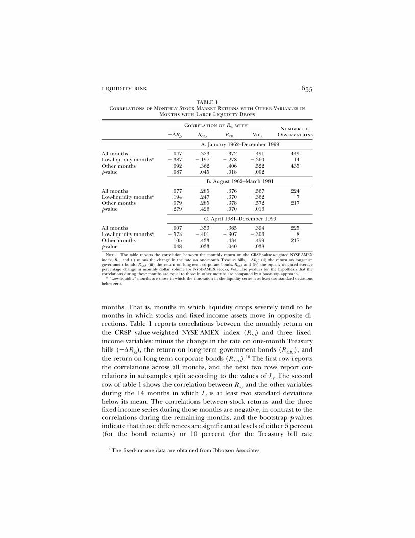
liquidity risk 655
TABLE 1Correlations of Monthly Stock Market Returns with Other Variables in
Months with Large Liquidity Drops
Correlation of withRS,t Number ofObservations�DRf,t RGB,t RCB,t Volt
A. January 1962–December 1999
All months .047 .323 .372 .491 449Low-liquidity months* �.387 �.197 �.278 �.360 14Other months .092 .362 .406 .522 435p-value .087 .045 .018 .002
B. August 1962–March 1981
All months .077 .285 .376 .567 224Low-liquidity months* �.194 .247 �.370 �.362 7Other months .079 .285 .378 .572 217p-value .279 .426 .070 .016
C. April 1981–December 1999
All months .007 .353 .365 .394 225Low-liquidity months* �.573 �.401 �.307 �.306 8Other months .105 .433 .434 .459 217p-value .048 .033 .040 .038
Note.—The table reports the correlation between the monthly return on the CRSP value-weighted NYSE-AMEXindex, and (i) minus the change in the rate on one-month Treasury bills, ; (ii) the return on long-termR , �DRS,t f,t
government bonds, ; (iii) the return on long-term corporate bonds, ; and (iv) the equally weighted averageR RGB,t CB,t
percentage change in monthly dollar volume for NYSE-AMEX stocks, Volt. The p-values for the hypothesis that thecorrelations during these months are equal to those in other months are computed by a bootstrap approach.
* “Low-liquidity” months are those in which the innovation in the liquidity series is at least two standard deviationsbelow zero.
months. That is, months in which liquidity drops severely tend to bemonths in which stocks and fixed-income assets move in opposite di-rections. Table 1 reports correlations between the monthly return onthe CRSP value-weighted NYSE-AMEX index ( ) and three fixed-RS,t
income variables: minus the change in the rate on one-month Treasurybills ( ), the return on long-term government bonds ( ), and�DR Rf,t GB,t
the return on long-term corporate bonds ( ).16 The first row reportsR CB,t
the correlations across all months, and the next two rows report cor-relations in subsamples split according to the values of The secondL .trow of table 1 shows the correlation between and the other variablesRS,t
during the 14 months in which is at least two standard deviationsLt
below its mean. The correlations between stock returns and the threefixed-income series during those months are negative, in contrast to thecorrelations during the remaining months, and the bootstrap p-valuesindicate that those differences are significant at levels of either 5 percent(for the bond returns) or 10 percent (for the Treasury bill rate
16 The fixed-income data are obtained from Ibbotson Associates.
656 journal of political economy
change).17 The results across both subperiods generally support theinference drawn for the overall period, in that five of the six correlationsbetween and the fixed-income series are negative in the months ofRS,t
large liquidity drops.Also shown in table 1 is the correlation between the stock return
and the change in volume, Volt, defined as the equally weightedRS,t
average percentage change in monthly dollar volume for NYSE-AMEXstocks. Stock returns are positively correlated with volume changes inall months, but the correlation is negative in months with large liquiditydrops, and the bootstrap p-value for the overall period is .002. Thesubperiod results again support the inference that the correlation islower in the months of severe liquidity drops. There is no obvious storyhere, other than perhaps that, in such months, higher volume accom-panying a larger liquidity drop is another manifestation of a flight toquality. We also find that, in low-liquidity months, the correlation be-tween volume changes and is equal to �.27, whereas it equals .18 inLt
other months (and in all months). But, again, we do not wish to pushthe descriptive analysis of the marketwide liquidity series too far. Theprimary goal of the paper is to investigate whether liquidity is a sourceof priced systematic risk in stock returns, and we use the series con-structed here for that purpose.
An important motive for entertaining a marketwide liquidity measureas a priced state variable is evidence that fluctuations in liquidity exhibitcommonality across stocks. Chordia, Roll, and Subrahmanyam (2000)and Huberman and Halka (2001) find significant commonality in var-ious liquidity measures at a daily frequency, whereas Hasbrouck andSeppi (2001) find only weak commonality in intraday (15-minute) fluc-tuations in liquidity. Our stock-by-stock measure affords an additionalgit
perspective on commonality, since it measures liquidity differently, it isconstructed at a monthly frequency, and our sample period is substan-tially longer. We conduct a simple exploration of commonality in git
across stocks by first sorting all stocks at the end of each year by marketvalue and then assigning them to decile portfolios on the basis of NYSEbreak points (i.e., each decile has an equal number of NYSE stocks).Each decile portfolio’s change in liquidity for a given month is thencomputed as the cross-sectional average change in the individual-stockmeasures, and this procedure yields a 1963–99 monthly series of liquiditychanges for each decile. The sample correlation of these series betweenany two deciles is positive. If the decile series are averaged separatelyacross the odd-numbered and even-numbered deciles, the sample cor-relation between the two resulting series is .56, and the t-statistic for a
17 The p-values are computed by resampling the original series and then randomlyassigning observations to subsamples of the same size as in the reported results.
liquidity risk 657
test of zero correlation is 14.20. This commonality in our liquidity mea-sure across stocks enhances the prospect that marketwide liquidity rep-resents a priced source of risk.
C. Specification Issues
Our liquidity measure relies on a large cross section of stocks and yieldsa monthly series spanning more than 37 years. As such, the series seemswell suited for this study’s focus on liquidity risk and asset pricing.Aggregate stock market liquidity is measured in a variety of alternativeways by recent studies that explore other interesting issues. Those studiesinclude Chordia, Roll, and Subrahmanyam (2000, 2001, 2002), Lo andWang (2000), Amihud (2002), and Jones (2002). Chordia, Roll, andSubrahmanyam form daily time series of various measures of liquidity(such as depth and bid-ask spread) and trading activity (such as dollarvolume), averaged across NYSE stocks over the period 1988–98. Lo andWang form a weekly series of average turnover across NYSE and AMEXstocks from July 1962 to December 1996. Amihud constructs an annualaggregate liquidity series for the period 1963–97 by averaging acrossNYSE stocks the ratios of average absolute price change to trading vol-ume. Jones collects an annual time series of average quoted bid-askspreads on the stocks in the Dow Jones index, covering the period1898–1998.
While measures of trading activity such as volume and turnover seemuseful in explaining cross-sectional differences in liquidity, they do notappear to capture time variation in liquidity. Although liquid marketsare typically associated with high levels of trading activity, it is often thecase that volume is high when liquidity is low. One example is October19, 1987, when the market was highly illiquid in many respects buttrading volume on the NYSE set its historical record. More generally,the previous subsection shows that the positive time-series correlationbetween our liquidity measure and dollar volume turns negative whencalculated only across low-liquidity months. For this reason, we do notproxy for time variation in liquidity using measures of trading activity.Bid-ask spreads and depth are not used either because suitable data arenot available for a long enough sample period. The data of Chordia,Roll, and Subrahmanyam span 11 years, which is too short for an assetpricing study. Notably, their liquidity measures (quoted share and dollardepth, quoted absolute and proportional spreads, and effective absoluteand proportional spreads) covary with ours in the expected direction(depth positively and spreads negatively). These measures are also jointlysignificant in explaining the time variation in our measure, as one might
658 journal of political economy
expect from measures that capture different dimensions of marketliquidity.18
As explained earlier, our liquidity measure reflects reversals in returnsin excess of the market. Another potential source of negative serialcorrelation in excess returns is nonsynchronous trading. (When returnsare measured with reported closing prices, an infrequently traded se-curity is more likely to outperform the market on a day following oneon which it underperforms.) With nonsynchronous trading, however, areversal on day is more likely when volume on day d is low, asd � 1opposed to high as under the liquidity interpretation of in (1). More-gi,t
over, nonsynchronous trading is likely to be more important when trad-ing activity is low, but we find that average turnover is in fact slightlyhigher in the months identified as having the lowest liquidity by ourmeasure. Nevertheless, it remains possible that nonsynchronous tradingmakes some contribution to a negative value of If the negative serialg .i,t
correlation in excess returns, arising from either liquidity-related re-versals or nonsynchronous trading, is relatively more stable through timethan volatility, then fluctuations in volatility are likely to be reflected inthe value of Recall from the earlier discussion that our aggregateg .i,t
liquidity series exhibits a negative association with market volatility.The liquidity measure used in this paper has substantial ex ante appeal
and a number of empirical liquidity-like features, as argued earlier. Oneclass of alternative measures involves merely changing the precise spec-ification of regression (1). In fact, one can consider 24 different spec-ifications (including ours). The variable on the left-hand side of (1) canbe either the excess or total stock return. On the right-hand side, thefirst regressor can be either total return or excess return, or it can beabsent. Next, one can use not only excess return but also total returnto sign volume for the purpose of obtaining a proxy for order flow.Finally, the return sign can be replaced by the return itself, for bothexcess and total return, motivated by the empirical implementation ofCampbell et al. (1993).
The various specifications described above produce aggregate seriesthat are all substantially different from ours. The correlations betweenthe innovations in the aggregate series produced by our specificationand those for the remaining 23 choices are low, ranging from �.47 to.80 and averaging .21. The highest correlation is achieved by the spec-ification that differs from ours only in replacing by itself.e esign(r ) ri,d,t i,d,t
The plot of the resulting series, shown in figure 2a, departs noticeably
18 Changes in our measure are regressed on changes in theirs in the overlapping periodof January 1988 through December 1998, excluding the change between June and July1997, when the quoted depth dropped sharply because of a reduction in the tick size onthe NYSE. The regression is .115, and the F-test rejects the hypothesis that all slopes2Rare jointly equal to zero with a p-value of .03.

liquidity risk 659
from the plot of our series in figure 1. For example, the well-knownlow-liquidity episodes of October 1987 and September 1998 are muchless prominent, and there are a number of downward spikes (e.g., inthe late 1990s) in months that are not commonly identified with low-liquidity events. Moreover, this alternative series does not exhibit theflight-to-quality effects documented for our measure in table 1: the stock-bond correlations in low-liquidity months are actually positive. Our li-quidity measure therefore seems more appealing than its most highlycorrelated alternative.
Figure 2 also plots the aggregate series for two other specificationsof regression (1) obtained by making only one change to ours. In figure2b, the lagged total return is replaced by its excess counterpartri,d,t
In figure 2c, the excess return is replaced by total return throughout,er .i,d,t
on the left-hand side as well as within the sign operator on the right-hand side. Both alternative series have a correlation of only .41 withours, and the flight-to-quality effects are again absent from both mea-sures. In addition, both series exhibit a negative correlation with themarket in negative-return months, in contrast to the significantly positivecorrelation obtained for our measure (.52) as well as for liquidity mea-sures such as bid-ask spreads and depth considered in other studies.Finally, the first series does not pick up the best-known low-liquidityperiods at all, and its time-series average is in fact positive, not negative.All these facts make the alternative specifications less appealing thanours.
Another test of the usefulness of the various alternative specificationsof (1) is to what extent they capture the liquidity effect modeled in thesimulation exercise described in Section IIA. To explore this issue, werepeated the simulation described there for each of the other 23 spec-ifications. The version with the same independent variables as ours buttotal returns on the left achieves the same correlation (.98) with thetrue liquidity value fi as our measure does. This is not surprising sincethe additional noise in the dependent variable under this alternativematters little in the population (large-sample) value for the slope. Moreinteresting is that all 22 remaining specifications produce smaller cor-relations with true liquidity, which lends additional support to our mea-sure as being a sensible specification relative to seemingly closealternatives.
Figure 2d plots the aggregate series obtained by value-weighting ourindividual stock measures across stocks. This series differs substantiallyfrom our equal-weighted measure, since the correlation between theinnovations in the two series is only .77. One less attractive feature ofthe value-weighted series is that certain months in which liquidity wasnotoriously low are relatively unimportant, largely because of the highvolatility of the series in the first half of the sample. When all months
660
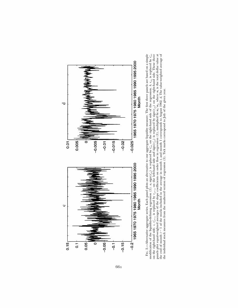
661
Fig
.2.—
Alt
ern
ativ
eag
greg
ate
seri
es.E
ach
pan
elpl
ots
anal
tern
ativ
eto
our
aggr
egat
eliq
uidi
tym
easu
re.T
he
firs
tth
ree
pan
els
are
base
don
asi
mpl
em
odifi
cati
onof
the
liqui
dity
-defi
nin
gre
gres
sion
(1).
a,is
repl
aced
byon
the
righ
t-han
dsi
deof
the
regr
essi
on.
b,is
repl
aced
bye
ee
sign
(r)
rr
ri,d
,ti,d
,ti,d
,ti,d
,t
onth
eri
ght-h
and
side
.c,
isre
plac
edby
onth
ele
ft-h
and
side
and
isre
plac
edby
onth
eri
ght-h
and
side
.T
hes
eth
ree
ee
rr
sign
(r)
sign
(r)
i,d�
1,t
i,d�
1,t
i,d,t
i,d,t
pan
els
plot
equa
l-wei
ghte
dav
erag
esof
the
slop
eco
effi
cien
tson
orde
rfl
owin
regr
essi
on(1
),m
ulti
plie
dby
wh
ere
isth
eto
tal
dolla
rva
lue
atm
/m,
mt
1t
the
end
ofm
onth
ofth
est
ocks
incl
uded
inth
eav
erag
ein
mon
tht,
and
mon
th1
corr
espo
nds
toA
ugus
t19
62.d
,T
he
valu
e-w
eigh
ted
aver
age
oft�
1th
ein
divi
dual
stoc
km
easu
res
from
the
unal
tere
dve
rsio
nof
regr
essi
on(1
).T
ick
mar
ksco
rres
pon
dto
July
ofth
egi
ven
year
.
662 journal of political economy
are sorted by their value-weighted liquidity measures, the October 1987liquidity crunch appears sixth and September 1998 appears only twenty-fifth in the order of importance. Moreover, the value-weighted seriesfails to exhibit any flight-to-quality effects: the correlations betweenstocks and bonds in low-liquidity months are in fact positive. Theseunappealing features of the value-weighted measure are likely due toits domination by large-cap stocks, whose liquidity often remains higheven when smaller-cap stocks experience a liquidity crunch. Our interestcenters on a broad liquidity measure, as opposed to a large-stock li-quidity measure, so we attempt to measure changes in aggregate liquidityusing an equally weighted average of the liquidity measures for individ-ual stocks.19
One might prefer to replace dollar volume on the right-hand side ofregression (1) by turnover, defined as dollar volume divided by marketcapitalization. Note that, with such a change, the resulting gamma co-efficients are very close to our coefficients multiplied by the stock’smarket cap at the beginning of the month, since the effects on theindependent variable of within-month variation in market cap are likelyto be small. Equal-weighting such modified gamma coefficients acrossstocks hence produces the same series as value-weighting our originalcoefficients and scaling them by the average market cap of all stocksused to compute the average. The resulting series therefore looks verysimilar to the series discussed in the previous paragraph, and it inheritsall the unappealing features of that series.
In summary, the various series produced by alternative specificationsand weightings of our regression-based liquidity measure are signifi-cantly different from our measure and exhibit various features thatrender them less appealing as measures of aggregate liquidity.
III. Is Liquidity Risk Priced?
This section investigates whether a stock’s expected return is related tothe sensitivity of its return to the innovation in aggregate liquidity, L .tThat sensitivity, denoted for stock i by its liquidity beta is the slopeLb ,i
coefficient on in a multiple regression in which the other independentLt
variables are additional factors considered important for asset pricing.To investigate whether the stock’s expected return is related to weLb ,i
follow a straightforward portfolio-based approach to create a universeof assets whose liquidity betas are sufficiently disperse. At the end ofeach year, starting with 1965, we sort stocks on the basis of their pre-dicted values of and form 10 portfolios. The postformation returnsLbi
19 We did repeat the historical beta analysis reported in table 8 below using the value-weighted series; the results are weaker but go in the same direction as those reported.
liquidity risk 663
on these portfolios during the next 12 months are linked across yearsto form a single return series for each decile portfolio. The excessreturns on those portfolios are then regressed on return-based factorsthat are commonly used in empirical asset pricing studies. To the extentthat the regression intercepts, or alphas, differ from zero, explainsLbi
a component of expected returns not captured by exposures to theother factors.
For the purpose of portfolio formation, we define as the coefficientLbi
on in a regression that also includes the three factors of Fama andLt
French (1993):
0 L M S Hr p b � b L � b MKT � b SMB � b HML � e , (9)i,t i i t i t i t i t i,t
where denotes asset i’s excess return, MKT denotes the excess returnri,t
on a broad market index, and the other two factors, SMB and HML,are payoffs on long-short spreads constructed by sorting stocks accordingto market capitalization and book-to-market ratio. This definition of
captures the asset’s comovement with aggregate liquidity that is dis-Lbi
tinct from its comovement with other commonly used factors. We allowfor any given stock to vary through time, and the predicted valuesLbi
of used to sort stocks are obtained using two methods. The first allowsLbi
the predicted to depend on the stock’s historical least-squares esti-Lbi
mate as well as a number of additional stock characteristics observableat the time of the sort. The results using that method, reported insubsection A, reveal large differences in expected returns on -sortedLbi
portfolios that are unexplained by the other factors. The second methoduses only historical betas and is presented to confirm that the first setof results is not driven solely by sorting stocks on the other characteristicsthat help predict liquidity betas. The results from that method, reportedin subsection B, also reveal large and significant differences in alphason the -sorted portfolios. Subsection C reports results obtained forLbi
portfolios formed by sorting stocks on market capitalization.Our analysis covers all stocks traded on the NYSE, AMEX, and
NASDAQ that are ordinary common shares (CRSP share codes 10 and11). Stocks with prices below $5 or above $1,000 are also excluded fromthe portfolio sorts. The portfolio formation procedure uses data avail-able only as of the formation date, and this requirement applies to theliquidity series as well. Thus the formation procedure each year beginswith a reestimation of (7) using only the raw liquidity series ( ) availablegt
up to that point in time. The historical values of used in that formationLt
year are then recomputed using (8), where is the fitted residual fromut
that reestimated regression.
664 journal of political economy
TABLE 2Determinants of Predicted Liquidity Betas
August 1962 through
December 1998 December 1983 December 1968
Intercept �1.79(�6.75)
�4.39(�12.94)
�2.75(�2.95)
Historical beta 2.30(9.97)
3.75(10.87)
9.18(9.99)
Average liquidity �.87(�4.12)
�.02(�.08)
�.48(�.61)
Average volume 1.54(3.29)
�3.37(�5.03)
.07(.05)
Cumulative return �.04(�.14)
1.00(2.86)
.93(.86)
Return volatility �.24(�1.60)
�1.13(�3.39)
�2.61(�2.25)
Price .59(1.85)
7.51(15.00)
4.32(3.38)
Shares outstanding �1.43(�3.37)
.67(1.26)
�.69(�.54)
Note.—Each column reports the results of estimating a linear relation between a stock’s liquidity beta and the sevencharacteristics listed (in addition to the intercept, shown first). At each year end shown, the estimation uses all stocksdefined as ordinary common shares traded on the NYSE, AMEX, or NASDAQ with at least three years of monthlyreturns continuing through the given year end. The estimation uses a two-stage pooled time-series and cross-sectionalapproach. Each value reported is equal to the coefficient estimate multiplied by the time-series average of the annualcross-sectional standard deviations of the characteristic. The t-statistics are in parentheses.
A. Sorting by Predicted Liquidity Betas
1. Predicting Liquidity Betas
We model each stock’s liquidity beta as a linear function of observablevariables
L ′b p w � w Z . (10)i,t�1 1,i 2,i i,t�1
The vector contains seven characteristics: (i) the historical liquidityZ i,t�1
beta estimated using all data available from months throught � 60(if at least 36 months are available), (ii) the average value of ˆt � 1 gi,t
from months through (iii) the natural log of the stock’st � 6 t � 1,average dollar volume from months through (iv) the cu-t � 6 t � 1,mulative return on the stock from months through (v) thet � 6 t � 1,standard deviation of the stock’s monthly return from months t � 6through (vi) the natural log of the price per share from montht � 1,
and (vii) the natural log of the number of shares outstandingt � 1,from month (These seven characteristics are listed in table 2.)t � 1.The list of characteristics is necessarily arbitrary, although they do pos-sess some appeal ex ante. Historical liquidity beta should be useful ifthe true beta is fairly stable over time. The average of the stock’s gi,t
and volume can matter if liquidity risk is related to liquidity per se.Stocks with different market capitalization could have different liquidity
liquidity risk 665
betas, so we include shares outstanding and stock price, whose productis equal to the stock’s market capitalization. The level and variability ofrecent returns simply allow some role for short-run return dynamics.Each characteristic is “demeaned” by subtracting the time-series average(through month ) of the characteristic’s cross-sectional average int � 1each previous month.
Substituting the right-hand side of (10) for in (9), we obtainLbi
0 M S Hr p b � b MKT � b SMB � b HMLi,t i i t i t i t
′� (w � w Z )L � e . (11)1,i 2,i i,t�1 t i,t
This regression for stock i contains 11 independent variables, seven ofwhich are cross products of the elements of with (This approachZ L .i,t�1 t
to incorporating time variation in betas follows Shanken [1990].) Toincrease precision in the face of the substantial variance in individual-stock returns, we restrict the coefficients and in equation (10)w w1,i 2,i
to be the same across all stocks and estimate them using the whole panelof stock returns. Specifically, at the end of each year between 1965 and1998, we first construct for each stock the historical series of
M S Hˆ ˆ ˆe p r � b MKT � b SMB � b HML , (12)i,t i,t i t i t i t
where the ’s are estimated from the regression of the stock’s excessb
returns on the Fama-French factors and using all data available upL ,tto the current year end. Then we run a pooled time-series, cross-sectionalregression of on the characteristics,ei,t
′e p w � w L � w Z L � n , (13)i,t 0 1 t 2 i,t�1 t i,t
again using all data available up to the current year end. The first yearend considered here is that of 1965, since the data on begin in AugustLt
1962, and it seems reasonable to use at least three years of data toconduct the estimation. A stock is excluded for any month in which ithas any missing characteristics.
Table 2 reports the estimated coefficients and from the pooledˆ ˆw w1 2
regression, together with their t-statistics.20 Results are reported for sev-eral periods, each beginning in August 1962 but ending in Decemberof a different year; the estimated coefficients are those used in theranking at that year end. Each coefficient is multiplied by the time-seriesaverage of the cross-sectional standard deviation of the correspondingdemeaned characteristic. This scaling helps clarify the relative contri-butions of the individual characteristics to the predicted betas. Historical
20 The t-statistics are computed assuming independence of the regression residuals,which are purged of common variation in returns attributable to the three Fama-Frenchfactors together with L .t
666 journal of political economy
liquidity beta is the most important determinant of the predicted betain the longest sample period, used for the most recent ranking in De-cember 1998. The coefficient of 2.30 ( ) indicates that if a stock’st p 9.97historical liquidity beta is one cross-sectional standard deviation abovethe cross-sectional mean of the historical betas, then the stock’s pre-dicted liquidity beta is higher by 2.30, when we hold the other char-acteristics constant and average the effect over time. Historical beta isalso the most robust determinant of the predicted beta across the dif-ferent periods. The coefficient on stock price is significantly positiveearly in the sample, but its effect weakens in the longer period. Volatilityenters negatively, again more strongly in the earlier periods. The co-efficients on the stock’s past return, shares outstanding, and averagevolume are less stable over time.21 The coefficient on the stock’s recentaverage is significantly negative in the longest period (and insignif-git
icantly negative in the subperiods), suggesting that stocks with lowerliquidity (as measured by ) tend to be more exposed to aggregategit
liquidity fluctuations.
2. Postranking Portfolio Betas
At the end of each year, stocks are sorted by their predicted liquiditybetas and assigned to 10 portfolios. The predicted beta for each stockis calculated from equation (10), using the year-end values of the stock’scharacteristics along with the values of and estimated using dataˆ ˆw w1 2
through the current year end. Portfolio returns are computed over thefollowing 12 months, after which the estimation/formation procedureis repeated. The postranking returns are linked across years, generatinga single return series for each decile covering the period from January1966 through December 1999. On average, there are 187 stocks in eachportfolio, and no portfolio ever contains fewer than 103 stocks.
Panel A of table 3 reports the postranking liquidity betas of the decileportfolios when the stocks within each portfolio are value-weighted.(The results for equally weighted portfolios, not shown, are nearly iden-tical.) The liquidity betas are estimated by running the regression in
21 As mentioned earlier, the trading volume of the NASDAQ stocks is overstated relativeto the NYSE/AMEX volume. When the NASDAQ stocks are excluded from the pooledregression, the coefficient on volume remains negative in the first two subperiods andturns insignificantly negative in the overall period. In addition, the results presented inthis section lead to similar conclusions about the relation between liquidity risk and ex-pected stock returns. We retain the NASDAQ stocks in the analysis because their inclusionincreases the dispersion of the postranking liquidity betas of the portfolios sorted onpredicted betas, in line with the purpose of the sorting procedure. Stocks with pricesoutside the $5–$1,000 range are also included in the pooled regression for the samereason: their inclusion increases the spread in the postranking betas, even if these stocksare subsequently excluded from the portfolio sorts.
TA
BL
E3
Pro
pert
ies
of
Port
foli
os
Sort
edo
nPr
edic
ted
Liq
uid
ity
Bet
as
Dec
ile
Port
foli
o
12
34
56
78
910
10–1
A.
Post
ran
kin
gL
iqui
dity
Bet
as
Jan
.19
66–D
ec.
1999
�5.
75(�
2.22
)�
6.54
(�2.
98)
�4.
66(�
2.59
)�
3.16
(�2.
18)
.90
(.69
)�
.63
(�.5
4)�
.86
(�.6
8).6
8(.
52)
2.44
(1.7
7)2.
48(1
.35)
8.23
(2.3
7)Ja
n.
1966
–Dec
.19
82�
7.28
(�1.
84)
�8.
29(�
2.54
)�
3.47
(�1.
19)
�3.
15(�
1.36
)2.
58(1
.23)
�.3
4(�
.17)
�.4
7(�
.22)
.73
(.33
)�
2.51
(�1.
10)
4.19
(1.3
8)11
.47
(2.0
6)Ja
n.
1983
–Dec
.19
99�
3.00
(�.8
5)�
4.27
(�1.
37)
�5.
09(�
2.12
)�
2.36
(�1.
22)
�1.
10(�
.63)
�.8
4(�
.57)
�1.
60(�
1.06
)1.
94(1
.22)
5.67
(3.2
3).8
5(.
36)
3.85
(.84
)
B.
Add
itio
nal
Prop
erti
es,J
anua
ry19
66–D
ecem
ber
1999
Mar
ket
cap
2.83
5.90
8.30
7.65
10.6
716
.61
15.9
916
.02
16.0
514
.28
Liq
uidi
ty�
.46
�.1
6�
.10
�.1
5�
.08
�.0
7�
.03
�.0
3�
.04
�.1
0M
KT
beta
1.24
(37.
70)
1.21
(44.
61)
1.09
(48.
31)
1.05
(56.
83)
1.04
(62.
83)
1.03
(68.
89)
1.00
(62.
56)
1.01
(60.
75)
.98
(55.
76)
.94
(40.
75)
�.3
0(�
6.85
)SM
Bbe
ta.7
0(1
4.47
).3
1(7
.64)
.05
(1.6
1).0
1(.
26)
�.0
9(�
3.51
)�
.12
(�5.
63)
�.1
2(�
5.04
)�
.09
(�3.
82)
�.1
2(�
4.76
).0
5(1
.36)
�.6
5(�
10.1
4)H
ML
beta
.07
(1.3
1).1
9(4
.36)
.23
(6.4
5).2
0(6
.69)
.11
(4.0
2).1
4(5
.68)
.08
(3.0
7)�
.00
(�.0
6)�
.01
(�.3
7)�
.34
(�9.
04)
�.4
0(�
5.74
)M
OM
beta
�.0
6(�
2.43
)�
.10
(�5.
35)
�.0
7(�
4.29
)�
.03
(�2.
19)
�.0
3(�
2.51
)�
.01
(�.7
2).0
1(.
53)
�.0
1(�
.72)
.03
(2.7
2).0
5(3
.02)
.11
(3.4
1)
No
te.—
At
each
year
end
betw
een
1965
and
1998
,el
igib
lest
ocks
are
sort
edin
to10
port
folio
sac
cord
ing
topr
edic
ted
liqui
dity
beta
s.T
he
beta
sar
eco
nst
ruct
edas
linea
rfu
nct
ion
sof
seve
nst
ock
char
acte
rist
ics
atth
ecu
rren
tye
aren
d,us
ing
coef
fici
ents
esti
mat
edfr
oma
pool
edti
me-
seri
es,c
ross
-sec
tion
alre
gres
sion
appr
oach
.Th
ees
tim
atio
nan
dso
rtin
gpr
oced
ure
atea
chye
aren
dus
eson
lyda
taav
aila
ble
atth
atti
me.
Elig
ible
stoc
ksar
ede
fin
edas
ordi
nar
yco
mm
onsh
ares
trad
edon
the
NYS
E,A
ME
X,o
rN
ASD
AQ
wit
hat
leas
tth
ree
year
sof
mon
thly
retu
rns
con
tin
uin
gth
roug
hth
ecu
rren
tye
aren
dan
dw
ith
stoc
kpr
ices
betw
een
$5an
d$1
,000
.T
he
port
folio
retu
rns
for
the
12po
stra
nki
ng
mon
ths
are
linke
dac
ross
year
sto
form
one
seri
esof
post
ran
kin
gre
turn
sfo
rea
chde
cile
.Pa
nel
Are
port
sth
ede
cile
port
folio
s’po
stra
nki
ng
liqui
dity
beta
s,es
tim
ated
byre
gres
sin
gth
eva
lue-
wei
ghte
dpo
rtfo
lioex
cess
retu
rns
onth
eag
greg
ate
liqui
dity
inn
ovat
ion
and
the
Fam
a-Fr
ench
fact
ors.
Pan
elB
repo
rtst
he
tim
e-se
ries
aver
ages
ofth
ede
cile
port
folio
s’m
arke
tca
pita
lizat
ion
and
liqui
dity
,obt
ain
edas
valu
e-w
eigh
ted
aver
ages
ofth
eco
rres
pon
din
gm
easu
res
acro
ssth
est
ocks
wit
hin
each
deci
le.M
arke
tca
pita
lizat
ion
isre
port
edin
billi
ons
ofdo
llars
.Ast
ock’
sliq
uidi
tyin
any
give
nm
onth
isth
esl
ope
coef
fici
ent
from
eq.(
1),m
ulti
plie
dby
100.
Als
ore
port
edar
epo
stra
nki
ng
gi,t
beta
sw
ith
resp
ect
toth
eth
ree
Fam
a-Fr
ench
fact
ors
and
am
omen
tum
fact
or,
esti
mat
edby
regr
essi
ng
valu
e-w
eigh
ted
port
folio
exce
ssre
turn
son
the
four
fact
ors.
Th
et-
stat
isti
csar
ein
pare
nth
eses
.
668 journal of political economy
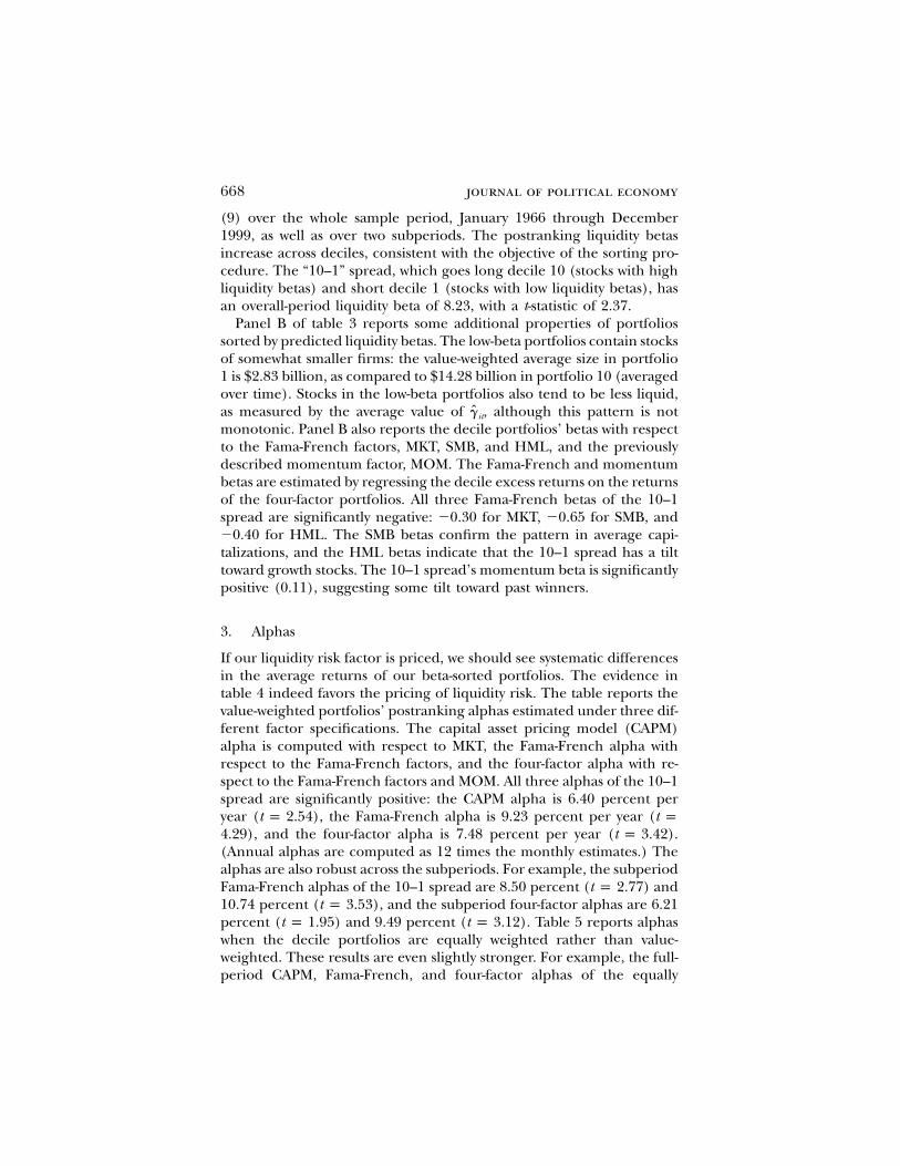
(9) over the whole sample period, January 1966 through December1999, as well as over two subperiods. The postranking liquidity betasincrease across deciles, consistent with the objective of the sorting pro-cedure. The “10–1” spread, which goes long decile 10 (stocks with highliquidity betas) and short decile 1 (stocks with low liquidity betas), hasan overall-period liquidity beta of 8.23, with a t-statistic of 2.37.
Panel B of table 3 reports some additional properties of portfoliossorted by predicted liquidity betas. The low-beta portfolios contain stocksof somewhat smaller firms: the value-weighted average size in portfolio1 is $2.83 billion, as compared to $14.28 billion in portfolio 10 (averagedover time). Stocks in the low-beta portfolios also tend to be less liquid,as measured by the average value of although this pattern is notg ,it
monotonic. Panel B also reports the decile portfolios’ betas with respectto the Fama-French factors, MKT, SMB, and HML, and the previouslydescribed momentum factor, MOM. The Fama-French and momentumbetas are estimated by regressing the decile excess returns on the returnsof the four-factor portfolios. All three Fama-French betas of the 10–1spread are significantly negative: �0.30 for MKT, �0.65 for SMB, and�0.40 for HML. The SMB betas confirm the pattern in average capi-talizations, and the HML betas indicate that the 10–1 spread has a tilttoward growth stocks. The 10–1 spread’s momentum beta is significantlypositive (0.11), suggesting some tilt toward past winners.
3. Alphas
If our liquidity risk factor is priced, we should see systematic differencesin the average returns of our beta-sorted portfolios. The evidence intable 4 indeed favors the pricing of liquidity risk. The table reports thevalue-weighted portfolios’ postranking alphas estimated under three dif-ferent factor specifications. The capital asset pricing model (CAPM)alpha is computed with respect to MKT, the Fama-French alpha withrespect to the Fama-French factors, and the four-factor alpha with re-spect to the Fama-French factors and MOM. All three alphas of the 10–1spread are significantly positive: the CAPM alpha is 6.40 percent peryear ( ), the Fama-French alpha is 9.23 percent per year (t p 2.54 t p
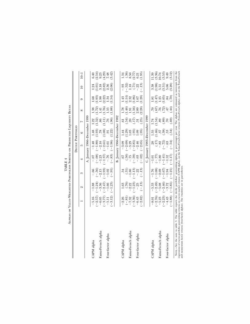
), and the four-factor alpha is 7.48 percent per year ( ).4.29 t p 3.42(Annual alphas are computed as 12 times the monthly estimates.) Thealphas are also robust across the subperiods. For example, the subperiodFama-French alphas of the 10–1 spread are 8.50 percent ( ) andt p 2.7710.74 percent ( ), and the subperiod four-factor alphas are 6.21t p 3.53percent ( ) and 9.49 percent ( ). Table 5 reports alphast p 1.95 t p 3.12when the decile portfolios are equally weighted rather than value-weighted. These results are even slightly stronger. For example, the full-period CAPM, Fama-French, and four-factor alphas of the equally
TA
BL
E4
Alp
has
of
Valu
e-W
eig
hte
dPo
rtfo
lio
sSo
rted
on
Pred
icte
dL
iqu
idit
yB
etas
Dec
ile
Port
foli
o
12
34
56
78
910
10–1
A.
Jan
uary
1966
–Dec
embe
r19
99
CA
PMal
pha
�5.
16(�
2.57
)�
1.88
(�1.
24)
�.6
6(�
.56)
�.0
7(�
.08)
�1.
48(�
1.80
)1.
48(1
.93)
1.22
(1.5
2)1.
38(1
.72)
1.68
(1.9
3)1.
24(1
.01)
6.40
(2.5
4)Fa
ma-
Fren
chal
pha
�6.
05(�
3.77
)�
3.36
(�2.
47)
�2.
15(�
1.93
)�
1.23
(�1.
37)
�2.
10(�
2.61
).7
8(1
.08)
.86
(1.1
1)1.
41(1
.76)
1.90
(2.2
2)3.
18(2
.82)
9.23
(4.2
9)Fo
ur-fa
ctor
alph
a�
5.11
(�3.
12)
�1.
66(�
1.23
)�
1.02
(�.9
1)�
.76
(�.8
3)�
1.61
(�1.
96)
.91
(1.2
2).7
6(.
96)
1.55
(1.8
8)1.
34(1
.54)
2.36
(2.0
6)7.
48(3
.42)
B.
Jan
uary
1966
–Dec
embe
r19
82
CA
PMal
pha
�2.
26(�
.81)
1.63
(.76
).5
4(.
31)
.67
(.50
)�
3.09
(�2.
69)
1.44
(1.2
9).6
1(.
54)
1.78
(1.4
6)1.
43(1
.14)
�.9
3(�
.52)
1.34
(.36
)Fa
ma-
Fren
chal
pha
�7.
32(�
3.36
)�
2.22
(�1.
23)
�1.
80(�
1.13
)�
.75
(�.5
9)�
3.29
(�2.
85)
1.03
(.95
).2
0(.
17)
1.91
(1.5
6)2.
32(1
.86)
1.18
(.71
)8.
50(2
.77)
Four
-fact
oral
pha
�6.
43(�
2.82
)�
.25
(�.1
3)�
.22
(�.1
3)�
.03
(�.0
2)�
2.46
(�2.
05)
1.09
(.95
).3
1(.
25)
2.89
(2.2
8)1.
67(1
.28)
�.2
2(�
.13)
6.21
(1.9
5)
C.
Jan
uary
1983
–Dec
embe
r19
99
CA
PMal
pha
�8.
01(�
2.76
)�
5.33
(�2.
49)
�1.
76(�
1.08
)�
1.01
(�.7
7).2
0(.
17)
1.55
(1.4
6)1.
74(1
.54)
.70
(.67
)1.
81(1
.47)
3.38
(1.9
8)11
.39
(3.3
6)Fa
ma-
Fren
chal
pha
�5.
23(�
2.23
)�
5.08
(�2.
46)
�2.
69(�
1.67
)�
1.80
(�1.
41)
�.8
2(�
.72)
.37
(.38
).8
9(.
89)
.76
(.72
)1.
25(1
.05)
5.51
(3.5
1)10
.74
(3.5
3)Fo
ur-fa
ctor
alph
a�
4.43
(�1.
88)
�3.
72(�
1.85
)�
1.94
(�1.
21)
�1.
52(�
1.17
)�
.63
(�.5
4).5
3(.
54)
.70
(.69
).4
7(.
44)
.84
(.70
)5.
06(3
.20)
9.49
(3.1
2)
No
te.—
See
the
not
eto
tabl
e3.
Th
eta
ble
repo
rts
the
deci
lepo
rtfo
lios’
post
ran
kin
gal
phas
,in
perc
enta
ges
per
year
.T
he
alph
asar
ees
tim
ated
asin
terc
epts
from
the
regr
essi
ons
ofex
cess
port
folio
post
ran
kin
gre
turn
son
exce
ssm
arke
tre
turn
s(C
APM
alph
a),o
nth
eFa
ma-
Fren
chfa
ctor
retu
rns
(Fam
a-Fr
ench
alph
a),a
nd
onth
eFa
ma-
Fren
chan
dm
omen
tum
fact
orre
turn
s(f
our-
fact
oral
phas
).T
he
t-sta
tist
ics
are
inpa
ren
thes
es.
TA
BL
E5
Alp
has
of
Eq
ual
lyW
eig
hte
dPo
rtfo
lio
sSo
rted
on
Pred
icte
dL
iqu
idit
yB
etas
Dec
ile
Port
foli
o
12
34
56
78
910
10–1
A.
Jan
uary
1966
–Dec
embe
r19
99
CA
PMal
pha
�5.
46(�
2.27
)�
1.47
(�.7
5)�
.73
(�.4
6).3
4(.
24)
.02
(.02
).9
4(.
84)
1.97
(1.9
1)2.
78(2
.71)
2.43
(2.3
7)2.
77(2
.06)
8.23
(4.1
2)Fa
ma-
Fren
chal
pha
�7.
53(�
6.35
)�
3.47
(�3.
39)
�3.
04(�
3.63
)�
1.58
(�2.
13)
�1.
67(�
2.47
)�
.76
(�1.
21)
.46
(.78
)1.
49(2
.50)
1.46
(2.1
8)2.
96(3
.14)
10.4
9(6
.50)
Four
-fact
oral
pha
�5.
80(�
4.98
)�
1.64
(�1.
68)
�1.
68(�
2.07
)�
.68
(�.9
2)�
1.02
(�1.
50)
�.1
7(�
.26)
.16
(.26
)1.
32(2
.16)
.95
(1.4
0)1.
86(1
.98)
7.66
(4.9
5)
B.
Jan
uary
1966
–Dec
embe
r19
82
CA
PMal
pha
1.74
(.49
)5.
52(1
.90)
5.22
(2.2
2)4.
49(2
.25)
2.99
(1.7
0)4.
15(2
.49)
4.76
(3.1
5)6.
00(4
.10)
4.11
(2.7
7)4.
68(2
.54)
2.95
(.98
)Fa
ma-
Fren
chal
pha
�6.
50(�
4.02
)�
1.12
(�.7
6)�
.80
(�.6
9)�
.51
(�.5
2)�
1.21
(�1.
25)
.02
(.02
)1.
12(1
.32)
2.70
(3.1
7)1.
23(1
.22)
2.76
(1.9
5)9.
25(4
.19)
Four
-fact
oral
pha
�5.
32(�
3.16
)1.
00(.
67)
1.28
(1.1
4).8
0(.
81)
.20
(.20
).9
3(1
.00)
.85
(.96
)2.
79(3
.12)
.84
(.79
)1.
18(.
81)
6.49
(2.9
1)
C.
Jan
uary
1983
–Dec
embe
r19
99
CA
PMal
pha
�11
.47
(�3.
70)
�7.
36(�
2.94
)�
6.09
(�2.
92)
�3.
06(�
1.63
)�
2.21
(�1.
41)
�1.
58(�
1.10
).0
6(.
04)
.29
(.21
)1.
77(1
.34)
1.78
(.92
)13
.25
(5.1
3)Fa
ma-
Fren
chal
pha
�8.
90(�
5.02
)�
5.83
(�4.
07)
�5.
58(�
4.62
)�
2.58
(�2.
26)
�2.
08(�
2.16
)�
1.56
(�1.
70)
.13
(.15
).5
4(.
64)
2.37
(2.7
2)4.
12(3
.33)
13.0
2(5
.50)
Four
-fact
oral
pha
�7.
10(�
4.40
)�
4.34
(�3.
35)
�4.
73(�
4.05
)�
2.00
(�1.
77)
�1.
92(�
1.97
)�
1.19
(�1.
30)
�.1
3(�
.15)
.29
(.34
)1.
87(2
.18)
3.42
(2.8
0)10
.51
(4.9
4)
No
te.—
See
the
not
eto
tabl
e3.
Th
eta
ble
repo
rts
the
deci
lepo
rtfo
lios’
post
ran
kin
gal
phas
,in
perc
enta
ges
per
year
.Th
eal
phas
are
esti
mat
edas
inte
rcep
tsfr
omth
ere
gres
sion
sof
exce
sspo
rtfo
liopo
stra
nki
ng
retu
rns
onex
cess
mar
ketr
etur
ns
(CA
PMal
pha)
,on
the
Fam
a-Fr
ench
fact
orre
turn
s(F
ama-
Fren
chal
pha)
,an
don
the
Fam
a-Fr
ench
and
mom
entu
mfa
ctor
retu
rns
(fou
r-fa
ctor
alph
as).
Th
et-s
tati
stic
sar
ein
pare
nth
eses
.
liquidity risk 671
weighted 10–1 spread are 8.23 percent, 10.49 percent, and 7.66 percent,respectively. The subperiod results are comparably strong, too.
We also test the hypothesis that all 10 alphas are jointly equal to zero,using the test of Gibbons, Ross, and Shanken (1989). For both equallyweighted and value-weighted portfolios and for all three models, thehypothesis is rejected at a 1 percent significance level in the overallperiod. The hypothesis is also rejected at the 5 percent level in bothsubperiods, for both equally weighted and value-weighted portfolios andfor all three models. The only exception occurs with the four-factoralphas for the value-weighted portfolios in the second subperiod, inwhich case the hypothesis is rejected at the 10 percent level.
Overall, the evidence strongly supports the hypothesis that our li-quidity risk factor is priced. The premium for this risk is positive, inthat stocks with higher sensitivity to aggregate liquidity shocks offerhigher expected returns. The latter result is consistent with the notionthat a pervasive drop in liquidity is seen as undesirable by the repre-sentative investor, so that the investor requires compensation for holdingstocks with greater exposure to this risk.
4. Estimating the Premium Using All 10 Portfolios
The discussion above relies on the 10–1 spread to infer that theexpected-return premium associated with liquidity risk is positive. Wealso estimate the liquidity risk premium using all 10 decile portfolios.Define the multivariate regression
Lr p b � BF � b L � e , (14)t 0 t t t
where rt is a vector containing the excess returns on the decile10 # 1portfolios; Ft is a vector containing the realizations of the “traded”4 # 1factors MKT, SMB, HML, and MOM; B is a matrix; and b0 and10 # 4
are vectors. We also consider a specification with only threeLb 10 # 1traded factors, excluding MOM. Assume that the decile portfolios arepriced by the returns’ sensitivities to the traded factors and the non-traded liquidity factor:
LE(r ) p Bl � b l , (15)t F L
where denotes the unconditional expectation. Taking expectationsE(7)of both sides of equation (14) and substituting from equation (15) gives
Lb p b [l � E(L )], (16)0 L t
since the vector of premia on the traded factors, is equal tol , E(F).F t
The liquidity factor is not the payoff on a traded position, so in generalLt
the liquidity risk premium is not equal to We estimate usingl E(L ). lL t L
the generalized method of moments (GMM) of Hansen (1982). Let v
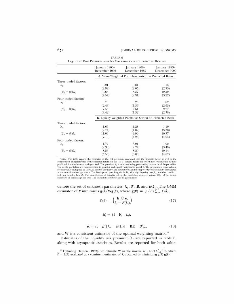
672 journal of political economy
TABLE 6Liquidity Risk Premium and Its Contribution to Expected Return
January 1966–December 1999
January 1966–December 1982
January 1983–December 1999
A. Value-Weighted Portfolios Sorted on Predicted Betas
Three traded factors:lL .91
(2.92).81
(2.05)1.13
(2.73)L L(b � b )l10 1 L 9.63
(4.57)8.37
(2.91)10.59(3.22)
Four traded factors:lL .78
(2.43).23
(1.36).82
(2.93)L L(b � b )l10 1 L 7.56
(3.42)2.61
(1.32)9.27
(2.78)
B. Equally Weighted Portfolios Sorted on Predicted Betas
Three traded factors:lL 1.65
(2.74)1.28
(1.82)1.10
(3.38)L L(b � b )l10 1 L 11.06
(7.19)9.90
(4.26)10.77(4.05)
Four traded factors:lL 1.72
(2.33)3.01(.74)
1.02(3.49)
L L(b � b )l10 1 L 8.56(5.53)
8.20(3.03)
10.14(4.07)
Note.—The table reports the estimates of the risk premium associated with the liquidity factor, as well as thecontribution of liquidity risk to the expected return on the “10–1” spread. Stocks are sorted into 10 portfolios by theirpredicted liquidity betas at each year end. The premium is estimated using postranking returns on all 10 portfolios.lL
The decile portfolios are value-weighted in panel A and equally weighted in panel B. The premium is reported as amonthly value multiplied by 1,200, so that the product of the liquidity beta and the reported premium can be interpretedas the annual percentage return. The 10–1 spread goes long decile 10, with high liquidity beta and short decile 1,Lb ,10
with low liquidity beta The contribution of liquidity risk to the portfolio’s expected return, is alsoL L Lb . (b � b )l ,1 10 1 L
expressed in percentage per year. The asymptotic t-statistics are in parentheses.
denote the set of unknown parameters: B, and The GMMLl , b , E(L ).L t
estimator of v minimizes where T′g(v) Wg(v), g(v) p (1/T)� f(v),ttp1
h � et tf(v) p , (17)t ( )L � E(L )t t
′ ′h p (1 F L ),t t t
L Le p r � b [l � E(L )] � BF � b L , (18)t t L t t t
and W is a consistent estimator of the optimal weighting matrix.22
Estimates of the liquidity risk premium are reported in table 6,lL
along with asymptotic t-statistics. Results are reported for both value-
22 Following Hansen (1982), we estimate W as the inverse of whereT ′ˆ ˆ(1/T)� f f ,t ttp1
evaluated at a consistent estimator of v, obtained by minimizing ′f p f (v) g(v) g(v).t t
liquidity risk 673
weighted and equally weighted portfolios. The full-period estimate ofis significantly positive for both sets of portfolios under both speci-lL
fications (three traded factors or four). The subperiod estimates are allpositive, and the majority are statistically significant. Overall, estimatingthe liquidity risk premium using all 10 portfolios confirms the previousinferences based on the extreme deciles.23 Again, liquidity risk appearsto be an economically important determinant of expected stock returns.
The magnitude of the liquidity risk premium depends on the ar-lL
bitrary scaling of described earlier, but that scaling does not affectLt
the t-statistic or the product the contribution of liquidity risk toLb l ,i L
asset i’s expected return. Table 6 also reports the GMM estimates ofthe difference between expected returns on the extremeL L(b � b )l ,10 1 L
decile portfolios implied by their liquidity betas. In the overall period,the annualized estimate of is 9.63 percent with three tradedL L(b � b )l10 1 L
factors and 7.56 percent with four (the corresponding values for equallyweighted portfolios are 11.06 percent and 8.56 percent). These valuesare close to the 10–1 spread alphas in table 4 of 9.23 percent and 7.48percent (the corresponding values in table 5 for equally weighted port-folios are 10.49 percent and 7.66 percent). Thus, even when the liquiditypremium is estimated using all 10 portfolios, the contribution of liquidityrisk to the 10–1 expected-return difference remains virtually unchanged.The contributions of the traded factors to the expected return of the10–1 spread are much smaller, all below 2 percent per year in absolutevalue for the overall period.
B. Sorting by Historical Liquidity Betas
As discussed earlier, a stock’s historical liquidity beta is the most im-portant predictor of its future liquidity beta (table 2). If liquidity betasare sufficiently stable over time, sorting on the historical liquidity betasalone could produce dispersion in the postranking betas. This subsec-tion shows that this is indeed the case, although the dispersion in thebetas is not as large as when liquidity betas are predicted using additionalvariables. Although our study focuses primarily on the results producedby sorts on betas predicted with the larger set of variables, we presenthere some results based on historical beta sorts in order to show thatthe results do not hinge on the inclusion of the additional variables.
At the end of each year between 1967 and 1998, we identify stockswith at least five years of monthly returns continuing through the currentyear end. For each stock, we estimate its historical liquidity beta byrunning the regression in (9) using the most recent five years of monthly
23 In no case does the asymptotic test reject the restriction in (15) at standard sig-2x
nificance levels.
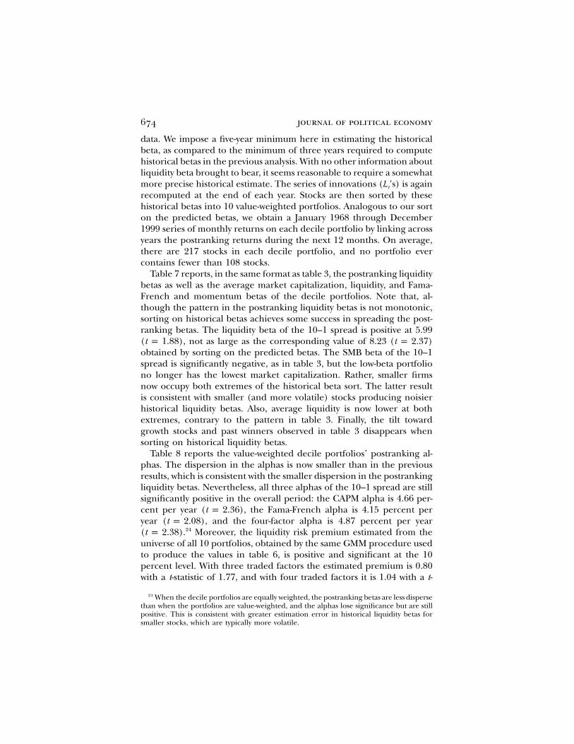
674 journal of political economy
data. We impose a five-year minimum here in estimating the historicalbeta, as compared to the minimum of three years required to computehistorical betas in the previous analysis. With no other information aboutliquidity beta brought to bear, it seems reasonable to require a somewhatmore precise historical estimate. The series of innovations ( ’s) is againLt
recomputed at the end of each year. Stocks are then sorted by thesehistorical betas into 10 value-weighted portfolios. Analogous to our sorton the predicted betas, we obtain a January 1968 through December1999 series of monthly returns on each decile portfolio by linking acrossyears the postranking returns during the next 12 months. On average,there are 217 stocks in each decile portfolio, and no portfolio evercontains fewer than 108 stocks.
Table 7 reports, in the same format as table 3, the postranking liquiditybetas as well as the average market capitalization, liquidity, and Fama-French and momentum betas of the decile portfolios. Note that, al-though the pattern in the postranking liquidity betas is not monotonic,sorting on historical betas achieves some success in spreading the post-ranking betas. The liquidity beta of the 10–1 spread is positive at 5.99( ), not as large as the corresponding value of 8.23 ( )t p 1.88 t p 2.37obtained by sorting on the predicted betas. The SMB beta of the 10–1spread is significantly negative, as in table 3, but the low-beta portfoliono longer has the lowest market capitalization. Rather, smaller firmsnow occupy both extremes of the historical beta sort. The latter resultis consistent with smaller (and more volatile) stocks producing noisierhistorical liquidity betas. Also, average liquidity is now lower at bothextremes, contrary to the pattern in table 3. Finally, the tilt towardgrowth stocks and past winners observed in table 3 disappears whensorting on historical liquidity betas.
Table 8 reports the value-weighted decile portfolios’ postranking al-phas. The dispersion in the alphas is now smaller than in the previousresults, which is consistent with the smaller dispersion in the postrankingliquidity betas. Nevertheless, all three alphas of the 10–1 spread are stillsignificantly positive in the overall period: the CAPM alpha is 4.66 per-cent per year ( ), the Fama-French alpha is 4.15 percent pert p 2.36year ( ), and the four-factor alpha is 4.87 percent per yeart p 2.08( ).24 Moreover, the liquidity risk premium estimated from thet p 2.38universe of all 10 portfolios, obtained by the same GMM procedure usedto produce the values in table 6, is positive and significant at the 10percent level. With three traded factors the estimated premium is 0.80with a t-statistic of 1.77, and with four traded factors it is 1.04 with a t-
24 When the decile portfolios are equally weighted, the postranking betas are less dispersethan when the portfolios are value-weighted, and the alphas lose significance but are stillpositive. This is consistent with greater estimation error in historical liquidity betas forsmaller stocks, which are typically more volatile.
TA
BL
E7
Pro
pert
ies
of
Port
foli
os
Sort
edo
nH
isto
rica
lL
iqu
idit
yB
etas
Dec
ile
Port
foli
o
12
34
56
78
910
10–1
A.
Liq
uidi
tyB
etas
Jan
.19
68–D
ec.
1999
�6.
02(�
2.57
)�
.65
(�.3
7)�
.62
(�.4
8)�
.54
(�.4
1)1.
12(.
96)
�1.
58(�
1.24
)1.
37(1
.00)
2.00
(1.4
9)3.
04(1
.99)
�.0
4(�
.02)
5.99
(1.8
8)Ja
n.
1968
–Dec
.19
83�
7.59
(�1.
84)
�1.
17(�
.44)
3.87
(1.8
6)�
1.54
(�.6
8)�
.48
(�.2
5)1.
65(.
71)
�1.
18(�
.55)
.02
(.01
)1.
26(.
54)
.41
(.14
)7.
99(1
.60)
Jan
.19
84–D
ec.
1999
�4.
17(�
1.52
)�
1.49
(�.6
3)�
4.10
(�2.
46)
�.3
0(�
.18)
2.55
(1.7
2)�
2.75
(�2.
00)
2.80
(1.5
6)3.
79(2
.08)
4.38
(2.0
7)1.
18(.
39)
5.35
(1.2
6)
B.
Add
itio
nal
Prop
erti
es,J
anua
ry19
68–D
ecem
ber
1999
Mar
ket
cap
7.11
7.69
10.4
417
.65
16.7
622
.18
16.2
611
.64
9.89
6.97
Liq
uidi
ty�
.52
�.1
9�
.06
�.0
4�
.02
�.0
5�
.05
�.0
5�
.05
�.1
2M
KT
beta
1.12
(37.
25)
1.09
(48.
37)
1.02
(61.
23)
.96
(56.
63)
.98
(65.
92)
.99
(59.
99)
1.02
(58.
01)
1.01
(58.
52)
1.02
(51.
53)
1.09
(40.
84)
�.0
3(�
.74)
SMB
beta
.37
(8.0
2)�
.00
(�.0
2)�
.13
(�5.
11)
�.1
6(�
6.03
)�
.09
(�4.
21)
�.1
5(�
6.10
)�
.11
(�4.
19)
�.0
0(�
.02)
.04
(1.2
0).1
6(4
.06)
�.2
0(�
3.25
)H
ML
beta
�.2
0(�
4.04
)�
.05
(�1.
31)
.02
(.87
)�
.02
(�.8
0).1
0(4
.22)
.12
(4.4
0).0
7(2
.60)
.09
(3.2
7)�
.01
(�.3
8)�
.15
(�3.
39)
.05
(.76
)M
OM
beta
.04
(1.6
4)�
.00
(�.1
8).0
2(1
.25)
.01
(1.1
3)�
.02
(�1.
91)
�.0
0(�
.17)
�.0
1(�
.76)
.01
(.65
)�
.02
(�1.
11)
�.0
1(�
.46)
�.0
5(�
1.51
)
No
te.—
At
each
year
end
betw
een
1967
and
1998
,el
igib
lest
ocks
are
sort
edin
to10
port
folio
sac
cord
ing
toh
isto
rica
lliq
uidi
tybe
tas.
Th
ebe
tas
are
esti
mat
edas
the
slop
eco
effi
cien
tson
the
aggr
egat
eliq
uidi
tyin
nov
atio
nin
regr
essi
ons
ofex
cess
stoc
kre
turn
son
that
inn
ovat
ion
and
the
thre
eFa
ma-
Fren
chfa
ctor
s.T
he
regr
essi
ons
are
esti
mat
edus
ing
the
mos
tre
cen
tfi
veye
ars
ofda
ta,
and
elig
ible
stoc
ksar
ede
fin
edas
ordi
nar
yco
mm
onsh
ares
trad
edon
the
NYS
E,
AM
EX
,or
NA
SDA
Qw
ith
five
year
sof
mon
thly
retu
rns
con
tin
uin
gth
roug
hth
ecu
rren
tye
aren
dan
dw
ith
stoc
kpr
ices
betw
een
$5an
d$1
,000
.T
he
port
folio
retu
rns
for
the
12po
stra
nki
ng
mon
ths
are
linke
dac
ross
year
sto
form
one
seri
esof
post
ran
kin
gre
turn
sfo
rea
chde
cile
.Pa
nel
Are
port
sth
ede
cile
port
folio
s’po
stra
nki
ng
liqui
dity
beta
s,es
tim
ated
byre
gres
sin
gva
lue-
wei
ghte
dpo
rtfo
lioex
cess
retu
rnso
nth
eliq
uidi
tyin
nov
atio
nan
dth
eFa
ma-
Fren
chfa
ctor
s.Pa
nel
Bre
port
sth
eti
me-
seri
esav
erag
esof
each
deci
le’s
mar
ketc
apit
aliz
atio
nan
dliq
uidi
ty,
obta
ined
asva
lue-
wei
ghte
dav
erag
esof
the
corr
espo
ndi
ng
mea
sure
sac
ross
the
stoc
ksw
ith
inea
chde
cile
.M
arke
tca
pita
lizat
ion
isre
port
edin
billi
ons
ofdo
llars
.A
stoc
k’s
liqui
dity
inan
ygi
ven
mon
this
the
slop
eco
effi
cien
tfr
omeq
.(1
),m
ulti
plie
dby
100.
Als
ore
port
edar
epo
stra
nki
ng
beta
sw
ith
resp
ect
toth
eFa
ma-
gi,t
Fren
chan
dm
omen
tum
fact
ors,
esti
mat
edby
regr
essi
ng
valu
e-w
eigh
ted
port
folio
exce
ssre
turn
son
the
four
fact
ors.
Th
et-s
tati
stic
sar
ein
pare
nth
eses
.
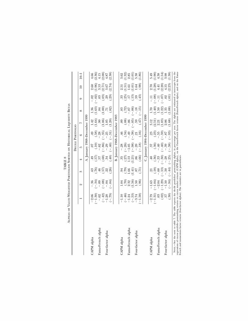
TA
BL
E8
Alp
has
of
Valu
e-W
eig
hte
dPo
rtfo
lio
sSo
rted
on
His
tori
cal
Liq
uid
ity
Bet
as
Dec
ile
Port
foli
o
12
34
56
78
910
10–1
A.
Jan
uary
1968
–Dec
embe
r19
99
CA
PMal
pha
�2.
06(�
1.30
)�
.36
(�.3
4).6
3(.
76)
.49
(.57
).0
7(.
10)
.49
(.58
)1.
42(1
.64)
1.36
(1.6
3)�
.02
(�.0
2)2.
60(1
.96)
4.66
(2.3
6)Fa
ma-
Fren
chal
pha
�.6
2(�
.42)
�.0
9(�
.08)
.46
(.57
).5
7(.
68)
�.6
2(�
.86)
�.2
8(�
.35)
.90
(1.0
6).8
4(1
.00)
.03
(.03
)3.
53(2
.71)
4.15
(2.0
8)Fo
ur-fa
ctor
alph
a�
1.20
(�.7
9)�
.04
(�.0
4).2
2(.
26)
.34
(.40
)�
.29
(�.4
0)�
.25
(�.3
1)1.
05(1
.20)
.71
(.82
).2
9(.
29)
3.67
(2.7
4)4.
87(2
.38)
B.
Jan
uary
1968
–Dec
embe
r19
83
CA
PMal
pha
�1.
10(�
.46)
1.04
(.70
).9
4(.
79)
.35
(.27
)�
.28
(�.2
6).4
6(.
34)
.09
(.08
).8
3(.
72)
.33
(.25
)2.
51(1
.51)
3.62
(1.3
2)Fa
ma-
Fren
chal
pha
�1.
24(�
.53)
2.32
(1.5
6)1.
66(1
.41)
1.53
(1.2
1)�
1.05
(�.9
8)�
.49
(�.3
8)�
.06
(�.0
5)�
.07
(�.0
6).1
7(.
13)
1.61
(1.0
1)2.
85(1
.01)
Four
-fact
oral
pha
�3.
74(�
1.58
)1.
50(.
96)
.87
(.71
).8
6(.
66)
�.2
0(�
.18)
.21
(.16
).5
9(.
47)
�.1
8(�
.15)
.59
(.43
)1.
64(.
98)
5.38
(1.8
6)
C.
Jan
uary
1984
–Dec
embe
r19
99
CA
PMal
pha
�2.
79(�
1.31
)�
1.63
(�1.
04)
.21
(.18
).4
0(.
36)
.37
(.36
).2
3(.
23)
3.12
(2.5
1)1.
70(1
.40)
�.1
1(�
.08)
2.70
(1.2
8)5.
49(1
.90)
Fam
a-Fr
ench
alph
a.0
3(.
02)
�2.
04(�
1.29
)�
.60
(�.5
3)�
.33
(�.3
0)�
.40
(�.4
0)�
.55
(�.5
9)2.
21(1
.83)
1.50
(1.2
2)�
.11
(�.0
7)4.
41(2
.20)
4.38
(1.5
4)Fo
ur-fa
ctor
alph
a.5
7(.
30)
�1.
50(�
.94)
�.5
0(�
.44)
�.2
8(�
.25)
�.3
9(�
.38)
�.8
7(�
.93)
2.06
(1.6
8)1.
35(1
.08)
.02
(.01
)4.
55(2
.23)
3.98
(1.3
8)
No
te.—
See
the
not
eto
tabl
e7.
Th
eta
ble
repo
rts
the
deci
lepo
rtfo
lios’
post
ran
kin
gal
phas
,in
perc
enta
gepe
rye
ar.
Th
eal
phas
are
esti
mat
edas
inte
rcep
tsfr
omth
ere
gres
sion
sof
exce
sspo
rtfo
liopo
stra
nki
ng
retu
rns
onex
cess
mar
ket
retu
rns
(CA
PMal
pha)
,on
the
Fam
a-Fr
ench
fact
orre
turn
s(F
ama-
Fren
chal
pha)
,an
don
the
Fam
a-Fr
ench
and
mom
entu
mfa
ctor
retu
rns
(fou
r-fa
ctor
alph
as).
Th
et-s
tati
stic
sar
ein
pare
nth
eses
.
liquidity risk 677
statistic of 1.76. Note that the magnitude of the premium in either caseis fairly close to its counterpart in table 6. In summary, the analysis basedsolely on historical betas supports the conclusion that stocks with greatersensitivity to innovations in aggregate liquidity offer higher expectedreturns.
C. Sorting by Size
Total market capitalization, or “size,” is a common criterion for sortingstocks in empirical investment studies, and size sorts often producedispersion in a number of other characteristics. Table 9 reports variousproperties of decile portfolios formed by sorting on size at the end ofeach year, where the break points are based on all eligible NYSE, AMEX,and NASDAQ stocks. Not surprisingly, smaller stocks are less liquid, inthat the average value of increases nearly monotonically acrossgit
deciles. The liquidity betas of the two or three portfolios containing thesmallest stocks are large and significantly positive, whereas the betas forthe other deciles exhibit no discernible pattern and are not significantlydifferent from zero. When the size sort is instead based on break pointsfor NYSE stocks only, so that each decile contains the same number ofNYSE stocks but more AMEX and NASDAQ stocks are assigned to thelower deciles, then the pattern in liquidity betas is fairly flat across all10 deciles, except for the large liquidity beta for the first decile. In otherwords, in a sort on size, the very smallest firms tend to be those withhigh liquidity betas.
It seems plausible that small and illiquid stocks might be those whosevalues are most affected by drops in marketwide liquidity, particularlyif those drops prompt some investors concerned with the overall li-quidity of their portfolios to “flee” such stocks and move to assets withgreater liquidity. At the same time, though, size and liquidity are notthe sole determinants of liquidity betas. Recall from table 3 that, whenwe sort by predicted liquidity betas, the high-beta portfolios actuallyhave somewhat higher liquidity and average market capitalizations thanthe low-beta portfolios. It is easy to see why stocks with high liquiditybetas need not be illiquid. When market liquidity declines, many in-vestors sell stocks and buy bonds (see table 1 for indirect evidence),and those investors might prefer to sell liquid stocks in order to saveon transaction costs. As a result, the price reaction to aggregate liquiditychanges could actually be stronger for stocks that are more liquid. Also,prices of liquid stocks could have greater sensitivity to aggregate liquidityshocks if such stocks are held in larger proportion by the more liquidity-conscious investors. In general, liquidity betas need not bear a simplerelation to size and liquidity.
Table 9 also reports the size-sorted portfolios’ alphas computed with
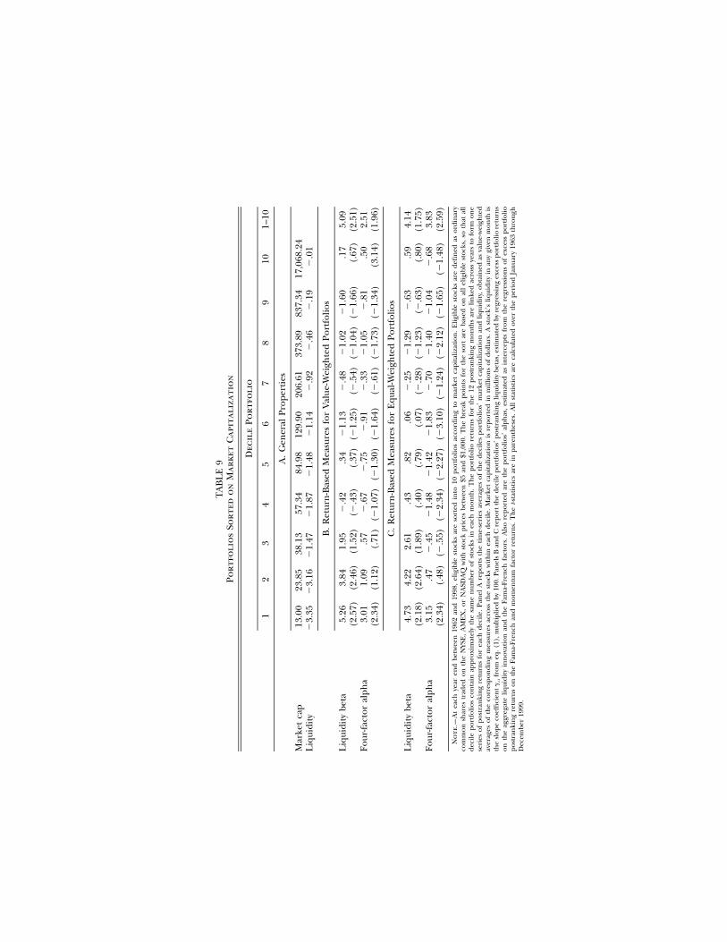
TA
BL
E9
Port
foli
os
Sort
edo
nM
arke
tC
apit
aliz
atio
n
Dec
ile
Port
foli
o
12
34
56
78
910
1–10
A.
Gen
eral
Prop
erti
es
Mar
ket
cap
13.0
023
.85
38.1
357
.34
84.9
812
9.90
206.
6137
3.89
837.
3417
,068
.24
Liq
uidi
ty�
3.35
�3.
16�
1.47
�1.
87�
1.48
�1.
14�
.92
�.4
6�
.19
�.0
1
B.
Ret
urn
-Bas
edM
easu
res
for
Val
ue-W
eigh
ted
Port
folio
s
Liq
uidi
tybe
ta5.
26(2
.57)
3.84
(2.4
6)1.
95(1
.52)
�.4
2(�
.43)
.34
(.37
)�
1.13
(�1.
25)
�.4
8(�
.54)
�1.
02(�
1.04
)�
1.60
(�1.
66)
.17
(.67
)5.
09(2
.51)
Four
-fact
oral
pha
3.01
(2.3
4)1.
09(1
.12)
.57
(.71
)�
.67
(�1.
07)
�.7
5(�
1.30
)�
.91
(�1.
64)
�.3
3(�
.61)
�1.
05(�
1.73
)�
.81
(�1.
34)
.50
(3.1
4)2.
51(1
.96)
C.
Ret
urn
-Bas
edM
easu
res
for
Equ
al-W
eigh
ted
Port
folio
s
Liq
uidi
tybe
ta4.
73(2
.18)
4.22
(2.6
4)2.
61(1
.89)
.43
(.40
).8
2(.
79)
.06
(.07
)�
.25
(�.2
8)�
1.29
(�1.
23)
�.6
3(�
.63)
.59
(.80
)4.
14(1
.75)
Four
-fact
oral
pha
3.15
(2.3
4).4
7(.
48)
�.4
5(�
.55)
�1.
48(�
2.34
)�
1.42
(�2.
27)
�1.
83(�
3.10
)�
.70
(�1.
24)
�1.
40(�
2.12
)�
1.04
(�1.
65)
�.6
8(�
1.48
)3.
83(2
.59)
No
te.—
At
each
year
end
betw
een
1962
and
1998
,el
igib
lest
ocks
are
sort
edin
to10
port
folio
sac
cord
ing
tom
arke
tca
pita
lizat
ion
.E
ligib
lest
ocks
are
defi
ned
asor
din
ary
com
mon
shar
estr
aded
onth
eN
YSE
,A
ME
X,
orN
ASD
AQ
wit
hst
ock
pric
esbe
twee
n$5
and
$1,0
00.
Th
ebr
eak
poin
tsfo
rth
eso
rtar
eba
sed
onal
lel
igib
lest
ocks
,so
that
all
deci
lepo
rtfo
lios
con
tain
appr
oxim
atel
yth
esa
me
num
ber
ofst
ocks
inea
chm
onth
.T
he
port
folio
retu
rns
for
the
12po
stra
nki
ng
mon
ths
are
linke
dac
ross
year
sto
form
one
seri
esof
post
ran
kin
gre
turn
sfo
rea
chde
cile
.Pa
nel
Are
port
sth
eti
me-
seri
esav
erag
esof
the
deci
les
port
folio
s’m
arke
tca
pita
lizat
ion
and
liqui
dity
,obt
ain
edas
valu
e-w
eigh
ted
aver
ages
ofth
eco
rres
pon
din
gm
easu
res
acro
ssth
est
ocks
wit
hin
each
deci
le.
Mar
ket
capi
taliz
atio
nis
repo
rted
inm
illio
ns
ofdo
llars
.Ast
ock’
sliq
uidi
tyin
any
give
nm
onth
isth
esl
ope
coef
fici
ent
from
eq.(
1),m
ulti
plie
dby
100.
Pan
els
Ban
dC
repo
rtth
ede
cile
port
folio
s’po
stra
nki
ng
liqui
dity
beta
s,es
tim
ated
byre
gres
sin
gex
cess
port
folio
retu
rns
gi,t
onth
eag
greg
ate
liqui
dity
inn
ovat
ion
and
the
Fam
a-Fr
ench
fact
ors.
Als
ore
port
edar
eth
epo
rtfo
lios’
alph
as,
esti
mat
edas
inte
rcep
tsfr
omth
ere
gres
sion
sof
exce
sspo
rtfo
liopo
stra
nki
ng
retu
rns
onth
eFa
ma-
Fren
chan
dm
omen
tum
fact
orre
turn
s.T
he
t-sta
tist
ics
are
inpa
ren
thes
es.
All
stat
isti
csar
eca
lcul
ated
over
the
peri
odJa
nua
ry19
63th
roug
hD
ecem
ber
1999
.
liquidity risk 679
respect to the four factors used previously (the excess market returnand size, value, and momentum spreads). Note that, for both the value-and equal-weighted portfolios, the estimated alpha for the decile ofsmallest firms is over 3 percent annually, with a t-statistic of 2.3. This 3percent positive abnormal return can be compared to the portion ofexpected return attributable to liquidity risk, computed as the productof the portfolio’s liquidity beta and the estimate of the liquidity riskpremium reported earlier. If we take the premium estimated usinglL
the value-weighted beta-sorted portfolios, reported in panel A in table6 (and the lower of the overall-period estimates), that product is 3.7percent ( ) for the equally weighted lowest-size decile andp 4.73 # 0.784.1 percent ( ) for the value-weighted version. In otherp 5.26 # 0.78words, the liquidity risk of the small-firm portfolio appears to be morethan sufficient to explain its abnormal return with respect to the otherfour factors.
D. Individual Stock Liquidity
This paper investigates whether the cross section of returns is relatedto stocks’ liquidity betas. A natural separate question is whether stockswhose liquidity is high according to our measure earn high averagereturns, in the spirit of Amihud and Mendelson (1986). This questioncannot be conclusively answered here. While our estimated liquiditymeasure seems appealing at the aggregate level, it is too noisy to beuseful at the individual stock level. In particular, when stocks are sortedinto 10 portfolios on the basis of their coefficients averaged over thegit
past one or three years, the pattern in the postranking portfolio ’s isg
rather flat across the deciles. The sorting procedure fails because of thelarge sampling error in the individual stock ’s. For this reason, we dogit
not work with individual stock liquidity. It seems that our most successfulsort on liquidity is the simple size sort described in the previoussubsection.
Our result that stocks with high liquidity betas tend to have highaverage returns does not appear to be explained by liquidity effects ala Amihud and Mendelson. Although the least liquid stocks in table 9tend to have the highest liquidity betas, recall that when stocks are sortedon their predicted liquidity betas, as in table 3, stocks with the highestliquidity betas actually have somewhat higher average postranking li-quidity measures than stocks with the smallest betas. The pricing resultsin tables 4 and 5 therefore seem distinct from any pure liquidity effects.
Given the mounting evidence on commonality in liquidity, it seemsnatural to ask whether the sensitivity of stock liquidity to market liquidityis related to the cross section of returns. This question is different fromthe one addressed in this paper, since stocks whose liquidities are the
680 journal of political economy
most sensitive to market liquidity are not necessarily those whose pricesare the most sensitive to market liquidity; the issue is of independentinterest nonetheless. One might conjecture, for example, that stockswhose liquidity dries up the most during marketwide liquidity crisesneed to compensate investors by higher average returns (e.g., Acharyaand Pedersen 2002). Our lack of reliable time series of liquidity forindividual stocks prevents us from investigating this hypothesis, sincesorts on betas (or correlations) of individual liquidity with respect toaggregate liquidity are unable to achieve any significant postrankingspread in those quantities. This intriguing topic presents an obviousdirection for future research.
IV. An Investment Perspective
The evidence presented in the previous section reveals that liquidityrisk is related to expected-return differences that are not explained bystocks’ sensitivities to MKT, SMB, HML, and MOM. An equivalent char-acterization of this evidence is that no combination of these four factors(and riskless cash) is mean-variance efficient with respect to the universeof common stocks.25 In particular, the large and significant alphas forthe 10–1 spreads reported in tables 4 and 5 imply that adding suchpositions to an opportunity set consisting of the other four factors in-creases the maximum Sharpe ratio.
In a linear pricing model in which expected returns are explainedby betas with respect to nontraded factors, expected returns are alsoexplained by betas with respect to portfolios whose returns are maxi-mally correlated with those factors.26 Constructing a maximum corre-lation portfolio for from the universe of common stocks is a chal-Lt
lenging problem that lies beyond the scope of this study. It is the casethat, if the ex post maximum correlation portfolio is constructed fromthe six-asset universe consisting of the first and last decile portfolios ofthe liquidity beta sort as well as the four factors MKT, SMB, HML, andMOM, then the weight on the high–liquidity beta portfolio is positiveand the weight on the low–liquidity beta portfolio is negative (for boththe value-weighted and equally weighted versions of those portfolios).In this sense, adding the 10–1 spread to an investment universe con-
25 The equivalence between multibeta asset pricing and mean-variance efficiency of somecombination of benchmark portfolios is well known. For an early recognition of this point,see Merton (1973); for later discussions, see Jobson and Korkie (1982, 1985), Grinblattand Titman (1987), and Huberman, Kandel, and Stambaugh (1987).
26 Huberman et al. (1987) characterize the “mimicking” portfolios that can be used inplace of nontraded factors when betas with respect to these factors explain expectedreturns.
liquidity risk 681
TABLE 10Liquidity Risk Spreads and Investment Opportunities: Weights in the Ex Post
Tangency Portfolio, January 1966–December 1999
MKT SMB HML MOM LIQV LIQE Sharpe Ratio
100.00 … … … … … .1235.08 5.83 59.10 … … … .2220.05 16.07 43.03 20.85 … … .3322.34 18.77 36.41 … 22.49 … .3117.32 22.33 29.10 … … 31.25 .4017.70 20.62 34.23 11.86 15.59 … .3715.88 22.51 29.56 6.47 … 25.58 .42
Note.—Each row reports the ex post tangency portfolio weights (percent) as well as the ex post monthly Sharperatio of the tangency portfolio in the given asset universe. The assets available for investment are various subsets of sixtraded factors. This set comprises the Fama-French factors MKT, SMB, and HML; a momentum factor MOM; and twoliquidity risk spreads, both of which go long decile 10, containing the stocks with the highest predicted liquidity betas,and short decile 1, containing the stocks with the lowest betas. Each leg of the spread is value-weighted in LIQV andequally weighted in LIQE.
sisting of the original four factors is motivated by a model in whichexpected returns are related to liquidity risk.
Let LIQV denote the payoff on the 10–1 spread constructed usingvalue-weighted decile portfolios sorted on predicted liquidity betas, andlet LIQE denote the payoff on the equally weighted version. To providean additional perspective on the importance of liquidity risk, we examinehere the degree to which the mean-variance opportunity set is enhancedby adding LIQV or LIQE to MKT, SMB, HML, and MOM. Of course, amean-variance-efficient portfolio is not necessarily the optimal choiceof an investor in a world that gives rise to multibeta pricing, but webelieve that a mean-variance setting is of interest to many investorsnevertheless. Table 10 reports, for the overall 1966–99 period, the max-imum ex post Sharpe ratio and the weights in the corresponding tan-gency portfolio for various subsets of the six factors. For ease of dis-cussion, let denote the maximum Sharpe ratio for a given set of∗Sassets. The original four factors have an of 0.33 (on a monthly basis).∗SWhen LIQV is added, increases to 0.37, and LIQV receives a greater∗Sweight in the ex post tangency portfolio than MOM (15.6 percent vs.11.9 percent). When LIQE is added to the original four, increases to∗S0.42, and the weight in MOM drops by more than two-thirds, from 20.9percent to 6.5 percent. In contrast, the weight on LIQE in that case is25.6 percent, which is higher than the weights on all but HML (29.6percent). Moreover, we see that when we add a fourth factor to thethree Fama-French factors, which by themselves have an of 0.22, LIQE∗Sis more valuable than MOM by the mean-variance comparison: LIQE
raises to 0.40 whereas MOM raises it to 0.33.∗SSince LIQV and LIQE figure prominently in the ex post tangency
portfolio, at the expense of MOM especially, we are led to investigatea bit further the extent to which the momentum factor’s importance is
682 journal of political economy
TABLE 11Liquidity Risk Spreads and Investment Opportunities: Alphas from the
Regression of Momentum on Portfolios Listed
January 1966–December 1999
January 1966–December 1982
January 1983–December 1999
MKT, SMB, HML 16.30(4.85)
21.65(4.53)
11.10(2.29)
MKT, SMB, HML, LIQV 13.89(4.09)
19.46(4.04)
8.03(1.63)
MKT, SMB, HML, LIQE 8.41(2.55)
16.11(3.35)
�1.29(�.28)
Note.—The table reports the alphas (percent per year) of the momentum portfolio MOM with respect to the factorslisted in each row. These factors include the Fama-French factors MKT, SMB, and HML and two liquidity risk spreads,both of which go long decile 10, containing the stocks with the highest predicted liquidity betas, and short decile 1,containing the stocks with the lowest betas. Each leg of the spread is value-weighted in LIQV and equally weighted inLIQE. The t-statistics are in parentheses.
reduced by our liquidity-risk spreads. Table 11 reports the alpha forMOM when regressed on the three Fama-French factors plus either LIQV
or LIQE. In the overall period, momentum’s annualized alpha with re-spect to just the three Fama-French factors is 16.3 percent with a t-statistic of 4.85, confirming a well-known result. Adding LIQV reducesMOM’s alpha somewhat, to 13.9 percent with a t-statistic of 4.09. Themomentum factor MOM is a spread between equally weighted portfo-lios, and perhaps for that reason the effect on its alpha of adding LIQE
to the Fama-French factors is more dramatic. That equally weightedliquidity risk spread cuts momentum’s full-period alpha nearly in half,to 8.4 percent with a t-statistic of 2.55. In the more recent 17-year sub-period from 1983 through 1999, MOM’s estimated alpha in the presenceof LIQE is actually negative, at �1.29.
Although such evidence is tantalizing, it is difficult to conclude thatliquidity risk provides a partial explanation for momentum. On onehand, MOM’s alpha is substantially reduced by the addition of liquidityrisk spreads, and MOM’s loadings on those spreads are highly significantin the overall period as well as in both subperiods (in the full period,MOM’s beta on LIQV is 0.26 with and MOM’s beta on LIQEt p 3.41,is 0.75 with in a multiple regression that includes the threet p 7.77,Fama-French factors). On the other hand, the liquidity beta of MOM,estimated as the multiple-regression coefficient on the nontraded factor
is positive but not statistically significant at conventional levels in theL ,toverall period (6.9 with a t-statistic of 1.3). Moreover, in the later sub-period, when LIQE eliminates MOM’s alpha, the estimated liquidity betaof MOM is negative (�1.65 with a t-statistic of �0.23). At the same time,though, we must remember that is at best an imperfect proxy forLt
whatever correct measure of liquidity could be relevant for asset pricing.It remains possible that the 10–1 spread constructed by ranking on betaswith respect to comes closer to the correct mimicking portfolio thanLt
liquidity risk 683
does to the correct liquidity measure. At this point, however, we canLt
simply observe that momentum’s importance in an investment contextis affected significantly by the addition of spreads based on liquidityrisk.
V. Conclusions
Marketwide liquidity appears to be a state variable that is important forpricing common stocks. We find that expected stock returns are relatedcross-sectionally to the sensitivities of stock returns to innovations inaggregate liquidity. Stocks that are more sensitive to aggregate liquidityhave substantially higher expected returns, even after we account forexposures to the market return as well as size, value, and momentumfactors.
Our liquidity measure captures a dimension of liquidity associatedwith the strength of volume-related return reversals. Over the last fourdecades, this measure of marketwide liquidity exhibits a number of sharpdeclines, many of which coincide with market downturns and apparentflights to quality. Our liquidity measure is also characterized by signif-icant commonality across stocks, supporting the notion of aggregateliquidity as a priced state variable. Smaller stocks are less liquid, ac-cording to our measure, and the smallest stocks have high sensitivitiesto aggregate liquidity.
One direction for future research is to explore whether liquidity riskplays a role in various pricing anomalies in financial markets. This studytakes a step on this path by showing that the momentum strategy ofbuying recent winning stocks and selling recent losing stocks becomesless attractive from an investment perspective when portfolio spreadsbased on liquidity risk are also available for investment. Future researchcould investigate whether expected returns are related to stocks’ sen-sitivities to fluctuations in other aspects of aggregate liquidity. It wouldalso be useful to explore whether some form of systematic liquidity riskis priced in other financial markets, such as fixed income markets orinternational equity markets.
References
Acharya, Viral V., and Pedersen, Lasse Heje. “Asset Pricing with Liquidity Risk.”Working paper. London: London Bus. School, 2002.
Amihud, Yakov. “Illiquidity and Stock Returns: Cross-Section and Time-SeriesEffects.” J. Financial Markets 5 (January 2002): 31–56.
Amihud, Yakov, and Mendelson, Haim. “Asset Pricing and the Bid-Ask Spread.”J. Financial Econ. 17 (December 1986): 223–49.
Amihud, Yakov; Mendelson, Haim; and Wood, Robert A. “Liquidity and the 1987Stock Market Crash.” J. Portfolio Management 16 (Spring 1990): 65–69.

684 journal of political economy
Brennan, Michael J.; Chordia, Tarun; and Subrahmanyam, Avanidhar. “Alter-native Factor Specifications, Security Characteristics, and the Cross-Section ofExpected Stock Returns.” J. Financial Econ. 49 (September 1998): 345–73.
Brennan, Michael J., and Subrahmanyam, Avanidhar. “Market Microstructureand Asset Pricing: On the Compensation for Illiquidity in Stock Returns.” J.Financial Econ. 41 (July 1996): 441–64.
Campbell, John Y.; Grossman, Sanford J.; and Wang, Jiang. “Trading Volumeand Serial Correlation in Stock Returns.” Q.J.E. 108 (November 1993): 905–39.
Chordia, Tarun; Roll, Richard; and Subrahmanyam, Avanidhar. “Commonalityin Liquidity.” J. Financial Econ. 56 (April 2000): 3–28.
———. “Market Liquidity and Trading Activity.” J. Finance 56 (April 2001):501–30.
———. “Order Imbalance, Liquidity, and Market Returns.” J. Financial Econ. 65(July 2002): 111–30.
Chordia, Tarun; Sarkar, Asani; and Subrahmanyam, Avanidhar. “An EmpiricalAnalysis of Stock and Bond Market Liquidity.” Working paper. Atlanta: EmoryUniv., 2002.
Chordia, Tarun; Subrahmanyam, Avanidhar; and Anshuman, V. Ravi. “TradingActivity and Expected Stock Returns.” J. Financial Econ. 59 (January 2001):3–32.
Constantinides, George M. “Capital Market Equilibrium with Transaction Costs.”J.P.E. 94 (August 1986): 842–62.
Datar, Vinay T.; Naik, Narayan Y.; and Radcliffe, Robert. “Liquidity and StockReturns: An Alternative Test.” J. Financial Markets 1 (August 1998): 203–19.
Eisfeldt, Andrea L. “Endogenous Liquidity in Asset Markets.” Working paper.Evanston, Ill.: Northwestern Univ., 2002.
Fama, Eugene F., and French, Kenneth R. “Common Risk Factors in the Returnson Stocks and Bonds.” J. Financial Econ. 33 (February 1993): 3–56.
———. “Multifactor Explanations of Asset Pricing Anomalies.” J. Finance 51(March 1996): 55–84.
Fiori, Filippo. “Liquidity Premia in the Equity Markets: An Investigation intothe Characteristics of Liquidity and Trading Activity.” Working paper. Chicago:Univ. Chicago, 2000.
Foster, F. Douglas, and Viswanathan, S. “Variations in Trading Volume, ReturnVolatility, and Trading Costs: Evidence on Recent Price Formation Models.”J. Finance 48 (March 1993): 187–211.
Gibbons, Michael R.; Ross, Stephen A.; and Shanken, Jay. “A Test of the Efficiencyof a Given Portfolio.” Econometrica 57 (September 1989): 1121–52.
Grinblatt, Mark, and Titman, Sheridan. “The Relation between Mean-VarianceEfficiency and Arbitrage Pricing.” J. Bus. 60 (January 1987): 97–112.
Grossman, Sanford J., and Miller, Merton H. “Liquidity and Market Structure.”J. Finance 43 (July 1988): 617–37.
Hansen, Lars Peter. “Large Sample Properties of Generalized Method of Mo-ments Estimators.” Econometrica 50 (July 1982): 1029–54.
Hasbrouck, Joel. “Measuring the Information Content of Stock Trades.” J. Finance46 (March 1991): 179–207.
Hasbrouck, Joel, and Seppi, Duane J. “Common Factors in Prices, Order Flows,and Liquidity.” J. Financial Econ. 59 (March 2001): 383–411.
Heaton, John, and Lucas, Deborah J. “Evaluating the Effects of IncompleteMarkets on Risk Sharing and Asset Pricing.” J.P.E. 104 (June 1996): 443–87.
Holmstrom, Bengt, and Tirole, Jean. “LAPM: A Liquidity-Based Asset PricingModel.” J. Finance 56 (October 2001): 1837–67.

liquidity risk 685
Huang, Ming. “Liquidity Shocks and Equilibrium Liquidity Premia.” J. Econ.Theory (in press).
Huberman, Gur, and Halka, Dominika. “Systematic Liquidity.” J. Financial Res.24 (Summer 2001): 161–78.
Huberman, Gur; Kandel, Shmuel; and Stambaugh, Robert F. “Mimicking Port-folios and Exact Arbitrage Pricing.” J. Finance 42 (March 1987): 1–9.
Jegadeesh, Narasimhan, and Titman, Sheridan. “Returns to Buying Winners andSelling Losers: Implications for Stock Market Efficiency.” J. Finance 48 (March1993): 65–91.
Jobson, John D., and Korkie, Bob. “Potential Performance and Tests of PortfolioEfficiency.” J. Financial Econ. 10 (December 1982): 433–66.
———. “Some Tests of Linear Asset Pricing with Multivariate Normality.” Ca-nadian J. Administrative Sci. 2, no. 1 (1985): 114–38.
Jones, Charles M. “A Century of Stock Market Liquidity and Trading Costs.”Working paper. New York: Columbia Univ., 2002.
Jorion, Philippe. “Risk Management Lessons from Long-Term Capital Manage-ment.” European Financial Management 6 (September 2000): 277–300.
Lee, Charles M. C., and Swaminathan, Bhaskaran. “Price Momentum and Trad-ing Volume.” J. Finance 55 (October 2000): 2017–69.
Llorente, Guillermo; Michaely, Roni; Saar, Gideon; and Wang, Jiang. “DynamicVolume-Return Relation of Individual Stocks.” Rev. Financial Studies 15 (Fall2002): 1005–47.
Lo, Andrew W.; Mamaysky, Harry; and Wang, Jiang. “Asset Prices and TradingVolume under Fixed Transaction Costs.” Working paper. Cambridge: Massa-chusetts Inst. Tech., 2001.
Lo, Andrew W., and Wang, Jiang. “Trading Volume: Definitions, Data Analysis,and Implications of Portfolio Theory.” Rev. Financial Studies 13 (Summer 2000):257–300.
Lowenstein, Roger. When Genius Failed: The Rise and Fall of Long-Term CapitalManagement. New York: Random House, 2000.
Lustig, Hanno. “The Market Price of Aggregate Risk and the Wealth Distribu-tion.” Working paper. Stanford, Calif.: Stanford Univ., 2001.
Merton, Robert C. “An Intertemporal Capital Asset Pricing Model.” Econometrica41 (September 1973): 867–87.
Shanken, Jay. “Intertemporal Asset Pricing: An Empirical Investigation.” J. Econ-ometrics 45 (July–August 1990): 99–120.
Vayanos, Dimitri. “Transaction Costs and Asset Prices: A Dynamic EquilibriumModel.” Rev. Financial Studies 11 (Spring 1998): 1–58.
Wang, Jiang. “A Model of Competitive Stock Trading Volume.” J.P.E. 102 (Feb-ruary 1994): 127–68.
“When the Sea Dries Up.” Economist 352 (September 25, 1999): 93.