the impact of day-trading on volatility and liquidity* - apjfs.org
TRANSCRIPT

Asia-Pacific Journal of Financial Studies (2009) v38 n2 pp237-275
237
The Impact of Day-Trading on Volatility and Liquidity*
Jay M. Chung University of Seoul, Seoul, Korea
Hyuk Choe
Seoul National University, Seoul, Korea
Bong-Chan Kho∗∗ Seoul National University, Seoul, Korea
Received 19 June 2007; Accepted 26 August 2008
Abstract
We examine day-trading activities for 540 stocks traded on the Korea Stock Exchange using transactions data for the period from 1999 to 2000. Our cross-sectional analysis reveals that day-traders prefer lower-priced, more liquid, and more volatile stocks. By estimating various bivariate VAR models using minute-by-minute data, we find that greater day-trading activity leads to greater return volatility and that the impact of a day-trading shock dissipates gradually within an hour. Past return volatility also positively affects future day-trading activity. We also find that past day-trading activity negatively affects bid-ask spreads, and past bid-ask spreads negatively affect future day-trading activity. Finally, we find that day-traders use short-term contrarian strategies and their order im-balance affects future returns positively. This result is consistent with a cyclical behavior of day-traders who concentrate their buy or sell trades at the bottom or peak of the short-term price cycles, respectively.
Keywords: Day-trading; Volatility; Liquidity; Contrarian; Momentum
* We are grateful for comments from seminar participants at the Ohio State University, the
Bowling Green State University, the Korea University, the Korea Securities Research In-stitute, and the Korea Finance Association meetings in 2003, as well as from Sung Bae, Jonathan Batten, Karl Diether, Kewei Hou, Andrew Karolyi, Kyoo Kim, Dong Wook Lee, Anil Makhija, Rodolfo Martell, René Stulz and two anonymous referees. Both the Institute of Management Research at Seoul National University (Choe and Kho) and the Research Fund #200704271032 at University of Seoul (Chung) provided financial support. Kho is also grateful for the Dice Center for Financial Economics at the Ohio State University, where part of this research was conducted. This paper is a part of a joint research project with the Korea Stock Exchange. However, it does not represent the view of the Korea Stock Ex-change, and the authors assume sole responsibilities for any error.
** Corresponding Author. Address: Seoul National University, College of Business Administra-tion, Kwanak-Gu, Sinlim-Dong, Seoul, Korea, 151-916; E-mail: [email protected]; Tel: +82-2-880-8798; Fax: +82-2-876-8411.
The Impact of Day-Trading on Volatility and Liquidity
238
1. Introduction
Since the late 1990s, the rise of the Internet has spurred a wave of online trading throughout the world and has led many ordinary individuals to engage in day-trading practices at a lower cost, which were once considered a domain solely for professional traders. Day-trading refers to an extremely active trading strategy in which traders move quickly in and out of stock positions to capture small profits on each trade. Typi-cal day-traders close out positions by the end of each trading day to avoid the risk associated with overnight price changes.
This paper examines the intraday impact of day-trading on return volatility and li-quidity. This topic is directly related to the current policy debate on whether day-trading exerts negative influences on the stock market. Although regulators in the U.S. are mostly concerned with securities law violations and business practices of day-trading firms, regulators in other countries are concerned more with the possibil-ity that day-trading may disrupt the market by increasing the volatility. To our knowledge, this topic has not been subject to thorough academic scrutiny, except for a few studies on day-traders’ profitability and Nasdaq’s Small Order Execution System (SOES),1) primarily due to the lack of data.
If day-trading trades occur randomly in a manner similar to that of other trades, there is little reason to believe that day-trading activity affects return volatility be-yond the normal impact of trading volume. However, if day-traders employ more or less similar strategies and respond to a common signal, they are likely to bunch up in certain periods, which may increase intraday return volatility. For example, suppose that most day-traders use momentum strategies as is widely believed.2) Since mo-mentum day-traders buy in upward moving markets and sell in downward moving markets, day-trading could magnify stock price fluctuations.
The impact of day-trading on liquidity depends on day-traders’ order submission strategies. While day-traders submitting limit orders provide liquidity, day-traders submitting market orders should be considered as consuming liquidity at the same
1) Some recent studies have looked at the profitability of day traders in countries where data is available;
Barber, Lee, Liu, and Odean (2004) for Taiwan, Linnainmaa (2005) for Finland, and Lee, Park, and Jang (2007) for Korea. They all show that day-traders tend to be reluctant to realize losses and perform not bet-ter than control groups on average. Due to such a disposition effect (Odean, 1999), the profitability of day-trading could be naturally biased upward, and we do not attempt to measure the profitability in this paper. SOES is designed originally for automatic routing and execution of small traders’ orders on Nasdaq.
2) For example, see Malkiel (August 3, 1999, The Wall Street Journal), ‘Day trading, and its dangers.’
Asia-Pacific Journal of Financial Studies (2009) v38 n2
239
time. In addition, the interactions between day-traders and other traders are also important. For example, if day-trading gets extremely prevalent, it may scare long-term investors away from the market, which may reduce liquidity. On the other hand, if day-traders act as merely uninformed traders chasing unwarranted price trends, they may entice savvy investors into trading to take advantage of those uninformed traders. Obviously, all of these issues are empirical questions as Barber and Odean (2001) summarize:
“Little is known about their [day traders’] trading strategies, because firms that cater to day traders have been generally reluctant to provide access to the trading records of their clients. Some day traders may add to market depth by providing instant liquidity, while those who try to profit from short-term momen-tum cycles probably increase market volatility. Which effect dominates remains an unresolved empirical question” (pp. 51-52).
Traders called ‘SOES bandits’ are generally also involved in day-trading because they seldom hold a position overnight.3) However, the day-trading we examine here is a recent and more general phenomenon. In essence, SOES bandits are artifacts of regulation unique to Nasdaq. The U.S. Securities and Exchange Commission (SEC) requires that broker-dealers on Nasdaq must honor at least five trades on SOES at a minimum size per trade at their current quote, which opens up the opportunity for SOES bandits to make profits. SOES bandits, who watch changes in different dealers’ quotes, identify short-term price trends and exploit dealers who are slow to adjust their quotes. On the other hand, day-trading in the Internet age has little to do with dealers and is a widespread phenomenon across many stock exchanges lacking either dealers or special regulations. In addition, while the SEC regulation limits the size of a SOES trade, there is no restriction on the size of day-trading trades. Nevertheless, we compare our results with the existing studies on active SOES trades because some of these studies share a common objective with our work. Using transactions data for a two-month period in 1995, Battalio, Hatch, and Jennings (1997) analyze the im-pacts of SOES trades on market volatility and find no evidence that SOES trades in-crease volatility beyond a one-minute interval. Harris and Schultz (1997) examine data for 20 large Nasdaq stocks for the period from November 1993 to March 1994
3) See Harris and Schultz (1998) for this issue.

The Impact of Day-Trading on Volatility and Liquidity
240
and find that SOES trades are more likely to be motivated by information. We use comprehensive transactions data for a two-year period from January 1999
to December 2000, obtained from the Korea Stock Exchange (KSE). The database is unique because it contains not only the complete history of orders and trades for all stocks traded on the KSE but also the account identification number for every order and trade, which is crucial for identification of day-trading trades. The KSE data are particularly suitable for our analyses because many investors are involved in short-term active trading during the sample period. The average turnover ratio on the KSE is ranked first in 1999 and third in 2000 among all stock exchanges in the world.4)
Here, we define day-trading in two ways. If an account buys and sells an equal number of shares for a stock on the same day, we call these trades ‘strict’ day-trading. If an account both buys and sells any numbers of shares for a stock on the same day, we call them ‘lenient’ day-trading. The second definition does not require the equality in the numbers of shares bought and sold and includes the first definition as a special case. Using these definitions, we find that day-trading is indeed popular in Korea during the sample period. For example, trades identified as strict day-trading ac-count for 11.0% of the total trading value in January 1999, and this proportion in-creases steadily to 20.8% in December 2000. Lenient day-trading trades account for 15.7% and 30.3% in January 1999 and December 2000, respectively.5)
Using a cross-sectional regression analysis, we find that day-traders prefer low price, liquid, and volatile stocks. First, day-traders prefer low price stocks mainly be-cause most of them are individuals armed with small amount of investment capital. The tax advantage of trading low price stocks in Korea may be another reason.6) Sec-ond, day-traders prefer liquid stocks (i.e., high volume stocks) probably because with liquid stocks they can exit from the market more easily. Day traders are less likely to
4) The ranks are obtained from the web site of the World Federation of Exchanges (http://www.world-
exchanges.org/). 5) These proportions are calculated in the same manner as done by the KSE. The KSE takes the smaller value
between the numbers of shares purchased and sold when calculating daily summary statistics of day-trading volume. Using this daily data from August 2000 to August 2001, Song (2003) estimates a daily bivariate VAR model and finds that past daily volatility strongly increases future day-trading volume whereas past day-trading only weakly affects future daily volatility. This weak impact of day-trading on volatility could be due to the fact that the impact is less likely to persist beyond one day because most day-traders seldom hold positions overnight. In this sense, it is necessary to focus on intra-day impacts of day-trading on volatility as in this paper.
6) Trading of stocks with a par value less than 5,000 won (roughly 5 U.S. dollars at an exchange rate of 1,000 won/U$) was exempted from the security transaction tax during the sample period. This tax exemption was abolished on June 28, 2001.
Asia-Pacific Journal of Financial Studies (2009) v38 n2
241
suffer from information asymmetry if they trade liquid stocks. Also, day-traders pre-fer volatile stocks through which they may have greater profit-making opportunities. Interestingly, day-traders do not seem to care much about systematic risks.
In order to analyze relations between day-trading activity and return volatility, we estimate a bivariate VAR model for each stock using minute-by-minute data. The VAR model includes many variables to control potential factors for day-trading and return volatility. We find that greater day-trading activity leads to greater return volatility, which is consistent with the conjecture made by Malkiel (1999) and Barber and Odean (2001). The impact of a day-trading shock dissipates gradually and be-comes statistically insignificant after an hour. This pattern is different from the re-sult in Battalio, Hatch, and Jennings (1997) in the U.S., who find no evidence that SOES trades increase volatility beyond a one-minute interval in a pooled regression model, and clearly demonstrates that the behavior of modern day-traders is different from that of SOES bandits. We also find that past return volatility also positively af-fects future day-trading activities, which is consistent with the evidence from the cross-sectional analysis.
We examine the relations between day-trading activity and liquidity by using a similar minute-by-minute VAR model and find that greater day-trading activity leads to lower bid-ask spreads, consistent with the argument that day-trading enhances market liquidity. We also find that day-trading activity becomes greater after the pe-riod of lower bid-ask spreads, which is consistent with the evidence from the cross-sec-tional regression analysis.
To understand the nature of day-trading behavior further, we estimate another bivariate VAR model. This model includes day-trading order imbalance and stock re-turns as dependent variables, both of which are signed variables. We find that day-traders use short-term contrarian strategies rather than momentum strategies and that past day-trading order imbalance appears to affect future returns positively for 15 minutes. This result is consistent with a cyclical behavior of day-traders who con-centrate their buy or sell trades at the bottom or peak of the short-term price cycles, respectively.
This paper proceeds as follows. Section 2 provides a brief description of the KSE as well as the data we use. Section 3 attempts to characterize the day-trading activities on the KSE. Section 4 presents the results from bivariate VAR models, which exam-ine the interactions between day-trading activities and volatility and those between day-trading activities and liquidity. Section 5 presents the results on the interactions

The Impact of Day-Trading on Volatility and Liquidity
242
between day-trading order imbalance and stock returns. This section also provides some evidence on whether day-trading activity destabilizes stock prices. Section 6 concludes this paper.
2. Data and day-trading variables
This section begins with a brief description of the KSE and proceeds to describe the data, the sample construction procedure, and the day-trading variables we use.
2.1 The Korea Stock Exchange (KSE)
The KSE is one of the most active stock markets in the world. Many investors in Korea are engaged in short-term trading strategies such as day-trading and have a relatively short investment horizon compared to investors in other countries. There are at least two reasons why short-term trading is popular in Korea. First, the use of online trading has been growing rapidly since 1999. As of December 2000, online trading accounts for 61.5% of the total stock trading value. The proportion of online trading was merely 1.3% in January 1998 and 4.7% in January 1999.7) Second, the popularity of short-term trading has been also spurred partly by low transaction costs of online trading in Korea. During the sample period, typical brokerage firms charge from 0.1% to 0.15% commissions for online trading while they charge 0.5% commis-sions for offline trading. Although traders must pay 0.3% of the proceeds from the sale of stocks as security transaction tax, trading stocks with prices less than the par value (typically 5,000 Korean won) are exempted from security transaction tax. Fur-ther, there are no capital gain taxes for trading exchange-listed stocks.
The KSE is a purely electronic limit-order market without designated market mak-ers. Investors can place either a limit or a market order, and all orders are directed to a centralized computer system, which matches orders according to the price and time priority rule. Since all limit orders are day orders, any unfilled outstanding limit or-der is cancelled automatically after the daily market closes. The KSE used batch auc-tions three times a day to determine the opening prices of the morning and afternoon sessions and the daily closing prices prior to May 22, 2000 on which daily lunch break 7) These numbers are from Chun (2001) published in Securities, a quarterly magazine published by the Korea
Securities Dealers’ Association. Barber and Odean (2002) also report nearly 19% of total retail investment assets of the U.S. households managed online.

Asia-Pacific Journal of Financial Studies (2009) v38 n2
243
(12:00-1:00 P.M.) was abolished. Since then, batch auctions have been used twice a day for the daily opening and closing prices. During the sample period, the KSE opens at 9:00 A.M. and closes at 3:00 P.M. In addition, the KSE adopts a 15% daily price limit system. In this system, stock prices on a day cannot rise above the 115% or fall below the 85% level of the previous closing price. If there is an event altering the number of outstanding shares such as stock dividends, splits, right offerings, etc., the exchange adjusts the previous closing price accordingly to determine the upper and lower bounds.
The KSE is a fairly transparent market. The KSE disseminated in real time the price and order quantities for the best bid and offer prior to April 1, 1997. On this day, the Exchange expanded the range of order disclosure to the best three bids and offers, and on March 27, 2000, it further expanded the range of order disclosure to the best five bids and offers.8) Since the majority of the stock investors on the KSE use online trading through a high-speed Internet, most investors can observe any change in or-ders within the range of order disclosure almost instantaneously. Furthermore, unlike many other limit-order markets in the world, the KSE does not allow ‘hidden orders.’ This should leave no room for uncertainty about disclosed order quantities.
2.2 Sample selection
The KSE data we use contain the complete history of orders and trades for all stocks traded on the KSE during the period from January 1999 to December 2000 (485 trading days). For each submitted order, detailed information is available in-cluding the order time in milliseconds, sequential order number, buy/sell indicator, order price and volume, market/limit order indicator, investor type, etc. For each trade, the data contain information on the trade time in milliseconds, sequential or-der number for each side of the trade, trade price and volume, etc. In addition, the data contain an account identification number for each order, which is the most unique feature of this data set enabling us to identify day-trading.9)
8) On January 2, 2002, the KSE started to disseminate the prices and order quantities for the best ten bids and
offers, but this event happened after the end of our sample period. 9) Because the Korean law prohibits the KSE from disseminating the information revealing the identity of an
account holder, each account identification number has been reassigned to a random number. However, the fake identification number is unique and consistent throughout the entire data. Thus, it is sufficient enough to distinguish an investor from another although we are unable to identify the demographic charac-teristics of the accounts.

The Impact of Day-Trading on Volatility and Liquidity
244
The data set is massive. It covers 745 common stocks, and the total number of ac-counts involved in at least one transaction during the sample period is 6,479,914.10) The total numbers of order records and trade records are 299,630,832 and 534, 761,255, respectively. Since we are conducting an intraday level analysis, we exclude inactive stocks from the sample. If the number of trading days with at least 10 trans-actions is less than 460 among the 485 trading days in the sample period, the stock gets also eliminated. As a result, the sample is reduced to 540 common stocks.
2.3 Defining day-trading
We use two definitions of day-trading: ‘strict’ and ‘lenient.’ Strict day-trading re-quires that the number of shares purchased must be the same as the number of shares sold for a stock on the same day. Thus, in this definition, day-traders are those who attempt to avoid the risk arising from the inability to trade overnight because they would not have any remaining positions by the end of the day. Formally, we de-fine strict day-trading as:
Definition I (Strict day-trading): If an account buys and sells an equal number of shares for a stock on the same day, these trades are all counted as strict day-trading trades.
The above definition is in line with the principle that most day-traders attempt to
follow. However, it may cause bias in our sample toward successful day-trading al-though it is unclear how the bias may affect the results of our analyses. Odean (1999), Barber and Odean (2000), and Choi, Laibson, and Metrick (2002) report that inves-tors tend to hold losing investments too long and sell winning investments too soon. If these results apply to day-traders, some day-traders may close out their positions by the end of the day when it turns out to be profitable, whereas they may leave the po-sition open for following days when deemed unprofitable. NASAA (1999) analyzes the transaction record from a day-trading firm and finds that most accounts are involved
10) This number is not the actual number of accounts. During the sample period, some member firms of the
Korea Stock Exchange have altered the account identification system. Thus, many accounts are counted twice.
Asia-Pacific Journal of Financial Studies (2009) v38 n2
245
in short-term trading but not in strict day-trading. Thus, we need to adopt an alter-native definition, namely ‘lenient day-trading’:
Definition II (Lenient day-trading): If an account both buys and sells any num-bers of shares of a stock on the same day, these trades are all counted as lenient day-trading trades.
The KSE adopts this definition when it publishes daily summary statistics on day-
trading since lenient day-trading includes strict day-trading as a special case. This definition also has a drawback, especially for an intraday analysis of profits. For in-stance, if an investor bought 1,000 shares at different prices on a day and sold 100 shares on the same day, it would be unclear which of the 1,000 shares were sold. Since both definitions have pros and cons, we take the view that they complement each other in our analysis.
In reality, however, investors may buy and sell shares on the same day without the intention of practicing day-trading. For example, an investor who bought 1,000 shares of a stock found another attractive stock later on the same day hence sold 100 shares of the 1,000 in order to have enough cash to buy the other stock. Such a case evi-dently challenges both definitions. However, there is no way of taking into account the intention of traders due to the intrinsic limitation of the data.
2.4 Measuring day-trading volume
This paper focuses on intraday analyses as the day-trading is essentially an intra-day phenomenon. Similar to Battalio, Hatch, and Jennings (1997), we look at the im-pact of day-trading volume on volatility (and liquidity) over one-minute intervals in a day. Once we identify day-trading accounts based on each of the two definitions ex-plained above, we measure their day-trading volume in each one-minute interval as follows.
Day-trading volume: In order to measure the intensity of day-trading volume relative to daily total trading volume for each stock, we calculate the following two measures over one-minute interval, both of which ignore the direction of trades:

The Impact of Day-Trading on Volatility and Liquidity
246
100%2
DTbuyfrq DTselfrqDTfrq
Frq+
= ××
(1)
100%2
DTbuyvol DTselvolDTvol
Vol+
= ××
, (2)
where DTbuyfrq and DTselfrq are buy and sell frequencies of day-trading during each one-minute interval for a stock, respectively, and Frq is the total frequency of trades for the stock on that day. Similarly, DTbuyvol and DTselvol are the buy and sell share volume of day-trading during each one-minute interval for a stock, respectively, and Vol is the total share volume traded for the stock on that day.
The day-trading volume measure (1) uses trading frequency similar to Battalio, Hatch, and Jennings (1997). In calculating trading frequency, we do not aggregate split trades originated from a market buy (sell) order that is greater than the depth of the best ask (bid). For example, if one large market order hits two limit orders sub-mitted by two day-traders, it is proper to count them as two day-trades for our pur-pose. Further, if one large market order submitted by a day-trader hits two existing limit orders, counting the trades as two day-trades is more appropriate because it better reflects the size of day-trading. Both measures (1) and (2) use the total volume of trades occurring on the same day as the denominator to normalize one-minute day-trading volume. Note here that we do not use the total volume of trades during the one-minute interval as the denominator since both measures would not behave prop-erly with a small trading volume during the interval.
Measuring lenient day-trading volume requires a special treatment because the numbers of shares bought and sold by an account do not need to be equal. For exam-ple, suppose that an investor sold 100 shares of a stock at 2:00 p.m., and the investor bought 100 shares of the stock at 10:00 a.m. and another 100 shares at 11:00 a.m. Since the investor bought and sold shares of the same stock in a day, he is classified as a day-trader. For the purpose of calculating daily summary statistics of day-trading volume, the smaller value between the numbers of shares bought and sold on the day, i.e., 100 shares in this case, should be counted toward the daily day-trading volume. This is the method used by the KSE, and we call it the KSE method. How-ever, for our intraday analysis over one-minute intervals, the 100 shares sold are counted toward DTselvol at 2:00 p.m., and each of the two 100 shares bought are counted toward DTbuyvol at 10:00 a.m. and 11:00 a.m., respectively. Note, however, that we cannot know whether the 100 shares sold were those purchased at 10:00 a.m.

Asia-Pacific Journal of Financial Studies (2009) v38 n2
247
or at 11:00 a.m.
Day-trading imbalance: To take into account the direction of day-trades, we es-timate day-trading imbalance over one-minute interval for each stock as follows:
100%DTbuyfrq DTselfrq
IDTfrqFrq−
= × (3)
100%,DTbuyvol DTselvol
IDTvolVol−
= × (4)
where the definitions of the symbols are exactly the same as before. These variables measure net purchases in terms of trading frequency and share volume, respectively.
3. The characteristics of day-trading
Literature on day-trading has been scarce due to the lack of comprehensive day-trading data. Even the most basic statistics are not available yet; thus, in this section, we briefly characterize day-trading activities on the KSE.
3.1 Patterns of day-trading activities
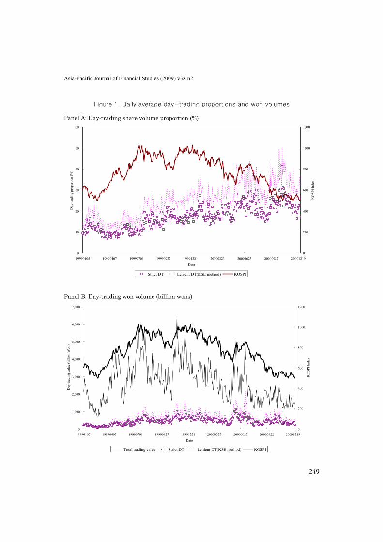
Table 1 presents descriptive statistics of day-trading activities in the sample. For each variable, we first calculate the mean over all trading days for each stock, and then aggregate cross-sectionally by averaging time-series means across the 540 sam-ple stocks. The results in Table 1 show that day-trading is very popular on the KSE. The strict day-trading in won volume, on average, amounts to 15.2% of the total trad-ing value. Lenient day-trading trades account for about 22.6% of the total trading value when day-trading value is measured by the KSE method. These numbers are invariant to the choice of the trading volume measures (won volume, trading frequency, or share volume). Figure 1 further shows that day-trading proportions based on share volume steadily increase during the sample period. Trades identified as strict day-trading ac-count for 11.0% of the total trading value in January 1999, and this proportion in-creases steadily to 20.8% in December 2000. Lenient day-trading trades account for 15.7% and 30.3% in January 1999 and December 2000, respectively.

The Impact of Day-Trading on Volatility and Liquidity
between day-trading order imbalance and stock returns. This section also provides some evidence on whether day-trading activity destabilizes stock prices. Section 6 concludes this paper.
2. Data and day-trading variables
This section begins with a brief description of the KSE and proceeds to describe the data, the sample construction procedure, and the day-trading variables we use.
The KSE is one of the most active stock markets in the world. Many investors in Korea are engaged in short-term trading strategies such as day-trading and have a relatively short investment horizon compared to investors in other countries. There are at least two reasons why short-term trading is popular in Korea. First, the use of online trading has been growing rapidly since 1999. As of December 2000, online trading accounts for 61.5% of the total stock trading value. The proportion of online trading was merely 1.3% in January 1998 and 4.7% in January 1999.7) Second, the popularity of short-term trading has been also spurred partly by low transaction costs of online trading in Korea. During the sample period, typical brokerage firms charge from 0.1% to 0.15% commissions for online trading while they charge 0.5% commis-sions for offline trading. Although traders must pay 0.3% of the proceeds from the sale of stocks as security transaction tax, trading stocks with prices less than the par value (typically 5,000 Korean won) are exempted from security transaction tax. Fur-ther, there are no capital gain taxes for trading exchange-listed stocks.
The KSE is a purely electronic limit-order market without designated market mak-ers. Investors can place either a limit or a market order, and all orders are directed to a centralized computer system, which matches orders according to the price and time priority rule. Since all limit orders are day orders, any unfilled outstanding limit or-der is cancelled automatically after the daily market closes. The KSE used batch auc-tions three times a day to determine the opening prices of the morning and afternoon sessions and the daily closing prices prior to May 22, 2000 on which daily lunch break
7) These numbers are from Chun (2001) published in Securities, a quarterly magazine published by the Korea Securities Dealers’ Association. Barber and Odean (2002) also report nearly 19% of total retail investment assets of the U.S. households managed online. Tw
o al
tern
ativ
e de
finiti
ons
of d
ay-t
radi
ng a
re u
sed
for
the
sum
mar
y st
atis
tics
belo
w. I
f an
acco
unt b
uys
and
sells
an
equa
l num
ber
of
shar
es fo
r a
stoc
k on
the
sam
e da
y, a
ll of
the
buy
and
sell
trad
es a
re c
lass
ified
as
stri
ct d
ay-tr
adin
g. If
an
acco
unt b
oth
buys
and
sel
ls
any
num
bers
of s
hare
s fo
r a
stoc
k on
the
sam
e da
y (b
uy a
nd s
ell v
olum
es n
eed
not b
e eq
ual),
all
of th
e bu
y an
d se
ll tr
ades
are
cla
ssi-
fied
as le
nien
t day
-tra
ding
. For
eac
h va
riab
le b
elow
, we
first
cal
cula
te d
aily
mea
ns o
ver
485
trad
ing
days
for
a st
ock,
and
then
, ave
r-ag
e th
em a
cros
s 54
0 sa
mpl
e st
ocks
. Rep
orte
d be
low
are
the
cro
ss-s
ectio
nal m
eans
and
sta
ndar
d de
viat
ions
(in
pare
nthe
ses)
. Mar
ket
orde
rs b
elow
inc
lude
mar
ket
orde
rs a
s w
ell
as l
imit
orde
rs t
hat
are
exec
utab
le i
mm
edia
tely
. The
KSE
met
hod
iden
tifie
s th
e da
y-tr
adin
g ac
coun
ts s
imila
r to
our
leni
ent d
ay-tr
adin
g, b
ut it
cal
cula
tes
daily
day
-trad
ing
volu
me
for
a st
ock
by ta
king
the
smal
ler
valu
e be
twee
n th
e bu
y an
d se
ll vo
lum
es o
rigi
nate
d fr
om e
ach
acco
unt.
St
rict
day
-tra
ding
Le
nien
t day
-tra
ding
Pu
rcha
ses
Sale
s Pu
rcha
ses
Sale
s K
SE m
etho
d
A: D
ay-t
radi
ng a
ctiv
ities
: Cro
ss-s
ectio
nal m
eans
(std
. dev
.)
Day
-tra
ding
freq
uenc
y 18
3.83
(3
57.7
2)18
3.37
(3
58.4
0)31
5.11
(6
03.8
9)30
3.62
(5
88.6
5)26
2.71
(5
15.4
8)
Prop
ortio
n re
lativ
e to
dai
ly to
tal (
%)
15.9
6 (4
.59)
15.9
2 (4
.72)
28.8
3 (7
.53)
27.9
1 (7
.64)
23.7
0
(6.5
8)
Day
-tra
ding
sha
re v
olum
e (1
,000
sha
res)
103.
16
(360
.19)
103.
16
(360
.19)
168.
90
(554
.39)
164.
39
(544
.23)
147.
32
(501
.22)
Prop
ortio
n re
lativ
e to
dai
ly to
tal (
%)
16.4
3 (5
.95)
16.4
3 (5
.95)
29.0
7 (9
.28)
28.0
8 (9
.20)
24.3
3
(8.3
8)
Day
-tra
ding
won
vol
ume
(mill
ion
won
s)83
6.76
(2
457.
88)
836.
76
(245
7.88
)14
30.0
9 (4
357.
64)
1385
.23
(423
2.10
)12
24.0
5 (
3724
.32)
Prop
ortio
n re
lativ
e to
dai
ly to
tal (
%)
15.1
8 (5
.57)
15.1
8 (5
.57)
27.0
0 (8
.99)
26.0
1 (8
.89)
22.5
7
(8.0
2)
B: P
ropo
rtio
n of
day
-tra
ding
freq
uenc
y by
ord
er ty
pes
(%):
Cro
ss-s
ectio
nal m
eans
(std
. dev
.)
Con
tinuo
us a
uctio
ns:
Mar
ket o
rder
trad
es
50.7
3 (2
.76)
52.6
9 (2
.54)
47.3
8 (2
.42)
50.9
3 (2
.21)
Non
-mar
keta
ble
limit
orde
r tr
ades
43
.27
(2.3
7)40
.75
(1.8
1)45
.86
(2.0
0)41
.59
(1.6
0)
Bat
ch a
uctio
n tr
ades
6.
01
(1.6
8)6.
56
(2.0
9)6.
76
(1.6
5)7.
48
(2.0
6)
Asia-Pacific Journal of Financial Studies (2009) v38 n2
249
Figure 1. Daily average day-trading proportions and won volumes
Panel A: Day-trading share volume proportion (%)
0
10
20
30
40
50
60
19990105 19990407 19990701 19990927 19991221 20000323 20000623 20000922 20001219
Date
Day
-trad
ing
prop
ortio
n (%
)
0
200
400
600
800
1000
1200
KO
SPI I
ndex
Strict DT Lenient DT(KSE method) KOSPI
Panel B: Day-trading won volume (billion wons)
0
1,000
2,000
3,000
4,000
5,000
6,000
7,000
19990105 19990407 19990701 19990927 19991221 20000323 20000623 20000922 20001219
Date
Day
-trad
ing
valu
e (b
illio
n W
on)
0
200
400
600
800
1000
1200K
OSP
I Ind
ex
Total trading value Strict DT Lenient DT(KSE method) KOSPI

The Impact of Day-Trading on Volatility and Liquidity
250
Although not reported in the table, the number of accounts with more than one strict day-trading in January 1999 turns out to be 107,329, which increases to 254,367 by December 1999, and then slightly falls back in December 2000 in response to the market decline. These figures are close to the estimate of 230,000 in the U.S. (ETA, 1999). The number of day-trading accounts with more than 100 days of strict day-trading in the year 1999 is 1,279, and it increases to 3,577 in the year 2000, indicat-ing that the number of ‘professional’ day-traders on the KSE is sizeable and compa-rable to the estimate of 5,000-7,000 in the U.S. as reported in ETA (1999) and the SEC (2000). We find these figures surprising because Korea is much smaller than the U.S. in terms of both size of the economy and population.
Also, we examine if day-trading activities are concentrated on only a few stocks. To do this, we draw the cross-sectional distribution of our 540 stocks’ daily average day-trading volume proportions relative to total trading values. Figure 2 shows the histo-gram, confirming that day-trading activities are a general phenomenon across sample stocks. For example, the median and the 25 percentile in the histogram of day-trading proportions are 14.3% (21.3%) and 11.4% (17.1%), respectively, when the definition of strict (lenient) day-trading is employed. The lowest strict (lenient) day-trading proportion is 3.6% (5.8%), and none of these sample stocks experience zero day-trading proportion.
In Figure 3, we plot average day-trading buy and sell volume proportions in each five-minute interval. To facilitate comparisons across time intervals, we divide each day-trading share volume by the total trading share volume on the day for the stock. For each five-minute interval, we calculate the daily average of day-trading volume proportions for each stock and then compute its average across our 540 sample stocks. We divide the sample period into two sub-periods; the first sub-period covers trading days prior to May 22, 2000, on which the KSE abolished the one-hour lunch break, and the second sub-period covers the subsequent period. Figure 3 reveals a striking asymmetry between buys and sells. Day-trading buy volume is the greatest in the opening batch auction period and decreases gradually. On the other hand, day-tra-ding sell volume increases gradually and is the greatest around the closing time. This intraday pattern is not surprising because day-traders attempt to trade out of their positions by the end of each trading day. However, we would like to note that this pattern is very different from the intraday pattern of the SOES trading volume,

Asia-Pacific Journal of Financial Studies (2009) v38 n2
251
Figure 2. Histogram of average day-trading volume proportions (in terms of shares)
Panel A: Strict day-trading
0
1
2
3
4
5
6
7
8
9
10
0 5 10 15 20 25 30 35 40
Day-trading proportions based on share volume (%)
Rel
ativ
e fr
eque
ncy
(%)
Panel B: Lenient day-trading (KSE method)
0
1
2
3
4
5
6
7
8
9
10
0 5 10 15 20 25 30 35 40 45 50
Day-trading proportions based on share volume (%)
Rel
ativ
e fre
quen
cy (%
)

The Impact of Day-Trading on Volatility and Liquidity
252
Figure 3. Intraday patterns of day-trading volume proportions
These figures present the average day-trading (strict day-trading) volume proportions in each five-minute interval for two sub-periods, where day-trading volume is measured in shares. In each five-minute interval, we first calculate the time-series averages of day-trading volume proportions, and then aggregate them by averaging across the sample stocks. For each stock, total number of shares traded on the day is used as the denominator in a day-trading volume proportion measure. Panel A: For the period with a lunch break of an hour (1999. 1. 4-2000. 5. 19: 341 days)
0
0.1
0.2
0.3
0.4
0.5
0.6
0.7
900 1000 1100 1150 1300 1400 1500
Time
Prop
ortio
n to
dai
ly to
tal v
olum
e (%
)
Buy Sell
Panel B: For the period with no lunch break (2000. 5. 22-2000. 12. 16: 149 days)
0
0.1
0.2
0.3
0.4
0.5
0.6
0.7
0.8
0.9
900 1000 1100 1200 1300 1400 1500
Time
Prop
ortio
n to
dai
ly to
tal v
olum
e (%
)
Buy Sell

Asia-Pacific Journal of Financial Studies (2009) v38 n2
253
which signifies the difference in trading strategies between SOES traders and gen-eral day-traders. Harris and Schultz (1998) report that SOES traders hold positions for very brief periods (5 minutes and 26 seconds, on average), and do not exhibit such an asymmetry between buys and sells.
3.2 Cross-sectional analysis of day-trading activities
In this subsection, we investigate whether day-trading activities vary across stocks with different stock characteristics. This analysis will provide us with a clue to the question of what kinds of stocks day-traders prefer. To measure day-trading activities, we apply the KSE method to day-trading trades identified as lenient day-trading. That is, for each stock, we calculate the time-series mean of daily day-trading share volume proportions in each calendar year. The time-series means calculated in this manner constitute the dependent variable in cross-sectional regressions. The explana-tory variables are as follows:
YR2000 : A year dummy variable; 0 for year 1999 and 1 for year 2000 Log PRC: The price level measured at the end of the previous year in KRW: log-
transformed FACE: A dummy variable representing the price level relative to the face value,
which takes 1 if more than 90% of the trading days in the year have clos-ing price less than the face value and 0 otherwise
Log SIZE: Total market value measured at the end of the previous year in million KRW: the number of outstanding shares times the price (log-transformed)
Log BM: The book-to-market ratio: previous year-end book value of common equity divided by SIZE (log-transformed)
BETA: The Dimson beta estimated in the previous year (weekly return data) Log VAL: Total trading volume in million KRW during the previous year (log-trans-
formed) VOLA: Time-series mean of daily high minus low volatility (%) in the previous
year To control for contemporaneous interactions between firm characteristic variables
and day-trading activities, we measure all the above variables, except for the year

The Impact of Day-Trading on Volatility and Liquidity
254
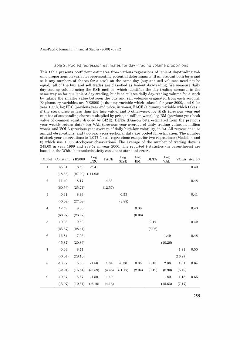
dummy variable, using the data from the previous year. All regressions use annual observations, and two-year cross-sectional data are pooled. The reported t-statistics are based on White heteroskedasticity consistent standard errors. Table 2 presents the results from nine cross-sectional regressions. The first seven models include only two explanatory variables one of which is the year dummy variable. The eighth model includes all explanatory variables, and the last model includes significant explana-tory variables only. Since changes in t-statistics for the coefficients of some variables show obvious interactions among explanatory variables, our discussion focuses on the last two regressions.
The adjusted R-squares in the last two regressions are 64% and 65%, respectively, indicating that these models perform quite well. The coefficient estimates show that the variables representing systematic risk, such as beta, firm size and book-to-mar-ket ratio. They may appear to be unimportant in determining day-trading activities, but the year dummy, price level, price level relative to the face value, trading volume, and volatility are main determinants of day-trading activities.11) This result suggests that day-traders are concerned more with firm-specific characteristics rather than systematic risks.
The significantly positive coefficient of the year dummy variable is consistent with the pattern observed in Figure 1. The price level variable has a significantly negative coefficient, which is not surprising because most of the day-traders are individual investors with relatively small amount of money. The significantly positive coefficient of a 0/1 dummy variable, FACE, shows that day-traders prefer stocks with a price less than the par value to take advantage of the exemption of security transaction taxes. The significantly positive coefficient of the trading volume variable indicates that day-traders prefer more liquid stocks. This is because day-traders can easily trade out of positions with liquid stocks, and because more liquid stocks are less likely to suffer from the problem of informational asymmetry among investors. The coefficient of the volatility variable is also significantly positive, indicating that vola-tile stocks are more likely to provide day-traders with profit-making opportunities. This is consistent with the notion that day-traders attempt to exploit short-term fluc-tuations in stock prices.
11) While we do not report in a table, we also ran daily cross-sectional regressions and obtained time-series
averages of the regression coefficients. The results were stronger, and the average R-squares increased up to the 68-70% range.
Asia-Pacific Journal of Financial Studies (2009) v38 n2
255
Table 2. Pooled regression estimates for day-trading volume proportions
This table presents coefficient estimates from various regressions of lenient day-trading vol-ume proportions on variables representing potential determinants. If an account both buys and sells any numbers of shares for a stock on the same day (buy and sell volumes need not be equal), all of the buy and sell trades are classified as lenient day-trading. We measure daily day-trading volume using the KSE method, which identifies the day-trading accounts in the same way as for our lenient day-trading, but it calculates daily day-trading volume for a stock by taking the smaller value between the buy and sell volumes originated from each account. Explanatory variables are YR2000 (a dummy variable which takes 1 for year 2000, and 0 for year 1999), log PRC (previous year end price, in wons), FACE (a dummy variable which takes 1 if the stock price is less than the face value, and 0 otherwise), log SIZE (previous year end number of outstanding shares multiplied by price, in million wons), log BM (previous year book value of common equity divided by SIZE), BETA (Dimson beta estimated from the previous year weekly return data), log VAL (previous year average of daily trading value, in million wons), and VOLA (previous year average of daily high-low volatility, in %). All regressions use annual observations, and two-year cross-sectional data are pooled for estimation. The number of stock-year observations is 1,077 for all regressions except for two regressions (Models 4 and 8) which use 1,036 stock-year observations. The average of the number of trading days is 245.09 in year 1999 and 238.52 in year 2000. The reported t-statistics (in parentheses) are based on the White heteroskedasticity consistent standard errors.
Model Constant YR2000 Log PRC FACE Log
SIZE Log BM BETA Log
VAL VOLA Adj. R2
1 35.04 8.59 -2.41 0.49
(18.56) (27.02) (-11.93)
2 11.49 8.17 4.35 0.48
(60.56) (25.71) (12.57)
3 -0.31 8.93 0.53 0.41
(-0.09) (27.08) (3.88)
4 12.59 9.00 0.08 0.40
(63.97) (26.07) (0.36)
5 10.36 9.53 2.17 0.42
(25.37) (28.41) (6.06)
6 -16.84 7.06 1.49 0.48
(-5.87) (20.86) (10.26)
7 -0.03 8.71 1.81 0.50
(-0.04) (28.10) (16.27)
8 -13.97 5.60 -1.56 1.64 -0.30 0.35 0.13 2.06 1.01 0.64
(-2.94) (15.54) (-5.59) (4.45) (-1.17) (2.04) (0.42) (8.93) (5.42)
9 -19.37 5.67 -1.50 1.49 1.89 1.15 0.65
(-5.07) (19.51) (-6.10) (4.13) (15.63) (7.17)
The Impact of Day-Trading on Volatility and Liquidity
256
4. The impact of day-trading on volatility and liquidity
In order to test whether day-trading activity affects return volatility or liquidity, we employ minute-by-minute bivariate VAR models. The VAR models enable us to test the Granger causality between day-trading activity and volatility and that be-tween day-trading activity and liquidity. Since investors do not know whether they are trading with day-traders or not, one may think there is little reason to believe that day-trading activity affects volatility and liquidity beyond the ‘normal’ impact of the increased trading volume. However, day-trading activity may affect volatility and liquidity, if day-traders herd as a group by using similar trading strategies. In fact, we have already caught a glimpse of day-traders’ systematic behavior in Figure 3. Day-trading buys are more likely to occur earlier and day-trading sells are more likely to occur later during a trading day.
4.1 Measuring volatility and liquidity
Similar to Battalio, Hatch, and Jennings (1997), we measure volatility as the log of the ratio of the highest bid-ask midpoint (Hi) to the lowest bid-ask midpoint (Lo) dur-ing each one-minute interval:
log( / ) 100%.= ×Volat Hi Lo (5)
We use bid-ask midpoints instead of transaction prices to avoid the influence of the bid-ask bounce on the volatility measure. We use bid-ask spreads as a proxy for li-quidity as follows:
100%,( ) / 2
−= ×
+
Ask BidSpread
Ask Bid (6)
where Ask and Bid are the prices of the best offer and bid, respectively.
4.2 The VAR framework
We set up bivariate VAR models to estimate the relationship between each pair of day-trading volume, volatility, and liquidity variables observed in one-minute inter-

Asia-Pacific Journal of Financial Studies (2009) v38 n2
257
vals. Specifically, when we analyze the relationship between day-trading volume and volatility, we use one of the two day-trading volume variables (DTfrq or DTvol) and the volatility variable (Volat) as dependent variables. For the relationship between day-trading volume and liquidity, we use Spread instead of Volat as a dependent variable. Each bivariate VAR model is set up for each stock in the sample and in-cludes 15 lags of the two dependent variables as explanatory variables and a number of control variables to control for the effects of other variables on day-trading volume, volatility, and liquidity. For example, the following is a representation of a bivariate system between day-trading volume and volatility:
15 15 5
, , , , , ,1 1 0
( )i t i i i t k i i t k i i t k i t i tk k k
x a b v c x d s f z ε− − −= = =
= + + + + +∑ ∑ ∑ (7)
15 15 5
, , , , , ,1 1 0
( ) ,i t i i i t k i i t k i i t k i t i tk k k
v v x s f zα β γ δ η− − −= = =
= + + + + +∑ ∑ ∑ (8)
where ,i tx denotes the day-trading volume variable (DTfrq or DTvol), ,i tv the volatility
variable (Volat), ,i ts the liquidity variable (Spread), and ,( )i tf z other control variables.12)
We use the following control variables: (1) Spread: This variable is used in the bivariate VAR system of day-trading volume
and volatility, to control for any remaining effect of bid-ask bounce on day-trading volume and return volatility. Both contemporaneous and 5 lagged variables are included.
(2) Volat: This variable is used in the bivariate VAR system of day-trading volume and liquidity, to control for the impact of return volatility on day-trading volume and liquidity. Both contemporaneous and 5 lagged variables are included.
12) This type of VAR model with control (or exogenous) variables is used in the literature, e.g., Pesaran and
Shin (1998), and Statman, Thorley, and Vorkink (2006). Especially, the latter sets up the VAR model for monthly data with the same lag length 10 for dependent variables and 2 for control variables across all sample stocks to facilitate the cross-sectional comparison of the coefficient estimates. Our lag selection is also made in the same spirit and uses the same but sufficiently long lags for all stocks since the use of lags sufficiently longer than optimal would not cause much problem associated with inconsistency, non-normality, or inefficiency given the large number of observations, 138,528 on average for each stock. [Lutkepohl (1999, Ch.4)] For 20 stocks randomly selected from each of trading volume decile and day-trading proportion decile, we perform the optimal lag search based on the Swartz Information Criterion (SIC) among various lag combinations from 1 through 30 for both dependent and control variables, and confirm that the optimal lag combinations for these variables are well within or equal to our choice of lags 15 and 5, respectively.

The Impact of Day-Trading on Volatility and Liquidity
258
(3) Trdfrq or Trdvol: These variables correspond to the use of DTfrq or Dtvol in the bivariate VAR system. Trdfrq is defined as the number of trades during each one-minute interval divided by the number of trades occurring during the day. Trdvol is defined as the share volume during each one-minute interval divided by the number of shares traded on the day. Both contemporaneous and 5 lagged vari-ables are included. They control for the normal effect of trading volume on volatil-ity and liquidity.
(4) Absmkt: This variable is a proxy for market volatility, defined as the absolute value of the one-minute log return on the nearest-term KOSPI 200 index futures. We use futures returns rather than the KOSPI returns because the latter may not reflect market movements instantaneously due to nonsynchronous trading of component stocks. Both contemporaneous and 5 lagged variables are included.
(5) DH1, …, DH6: These variables are time-of-day dummies representing each hour on a trading day, which are used to control for the well-known time-of-day pattern of volatility and liquidity. There are 5 hour-dummies (excluding DH4) for the pe-riod with a lunch break prior to May 22, 2000, and 6 hour-dummies for the subse-quent period with no lunch break.13) However, we do not include a dummy for the first hour (DH1) to avoid the linear dependence problem. No lagged dummy is in-cluded.
(6) Absdist: This variable is the absolute value of the log return calculated from the closing price on the previous day to the trading price observed at the end of the previous one-minute interval. Essentially, it measures the distance from the pre-vious closing price so that it can control for possible delay in the impact of trading on volatility in case the 15% price limit hits. No lag is included.
Table 3 presents summary statistics for the variables used in the bivariate VAR
models. It is easily noticeable that there are observations with exceptionally high values for most of the variables. For example, the maximum value is much higher than the 99.9 percentile value for most of the variables. In order to alleviate the im-pacts of these extreme values on the VAR model estimation, we set values greater than the 99.9 percentile to the value of the 99.9 percentile for each variable. We also check with the stationarity condition for all variables used in the VAR system based
13) Exclusion of these hour-dummies in the VAR estimation does not alter the main results.

Asia-Pacific Journal of Financial Studies (2009) v38 n2
259
on the Augmented Dickey-Fuller (ADF) and Phillips-Perron (PP) tests, and confirm that all variables satisfy the stationarity condition for each stock at the 1%, or at most, 10% significance level (not reported, but available upon request).
Table 3. Summary statistics of the variables used in VAR models of day-trading
activity and volatility (or liquidity)
If an account buys and sells an equal number of shares for a stock on the same day, all of the buy and sell trades are classified as strict day-trading. If an account both buys and sells any numbers of shares for a stock on the same day (buy and sell volumes need not be equal), all of the buy and sell trades are classified as lenient day-trading. We use one-minute interval to measure all variables used in the VAR models. For each variable reported below, we calculate the mean, standard deviations, and various percentile statistics across all one-minute intervals for each stock, and report cross-sectional averages of these statistics except for the maximum and minimum statistics, which are the maximum and minimum values across stocks. For each one-minute interval, DTfrq (%) is the average of the buy and sell frequencies divided by the number of trades occurring during the day, and DTvol (%) is the average of the buy and sell share volumes divided by the number of shares traded on the day. Volat (%) is the log of the ratio of the highest bid-ask midpoint to the lowest bid-ask midpoint during each one-minute interval. Spread (%) is the absolute bid-ask spread divided by the bid-ask midpoint. Trdfrq (%) is the number of trades during each one-minute interval divided by the number of trades oc-curring during the day, and Trdvol (%) is the share volume during each one-minute interval divided by the number of shares traded on the day. Absmkt (%) is the absolute value of the one-minute log return on the nearest-term KOSPI 200 futures contract. Absdist (%) is the ab-solute value of the log return calculated from the closing price on the previous day to the trad-ing price at the end of the previous one-minute interval.
Strict day-trading Lenient day-trading
DTfrq DTvol DTfrq DTvol Volat Spread Trdfrq Trdvol Absmkt Absdist
Mean 0.036 0.034 0.067 0.064 0.102 1.156 0.152 0.151 0.088 2.918
Std.dev. 0.144 0.195 0.229 0.316 0.275 0.934 0.392 0.532 0.089 2.795
Max 100.000 100.000 100.000 100.000 29.920 29.987 100.000 100.000 6.744 16.252
99.9% 1.677 2.090 2.561 3.438 2.697 7.406 4.171 6.237 0.679 15.057
75% 0.015 0.010 0.039 0.026 0.078 1.492 0.126 0.090 0.126 3.977
50% 0.002 0.001 0.006 0.003 0.009 0.904 0.028 0.017 0.071 2.127
25% 0.000 0.000 0.001 0.000 0.000 0.527 0.006 0.003 0.041 0.943
Min 0.000 0.000 0.000 0.000 0.000 0.000 0.000 0.000 0.000 0.000
We estimate the bivariate VAR models separately for each of 540 stocks.14) For a
variable with lags, we report the sum of coefficient estimates of all lagged variables 14) To avoid crossing day boundaries, we stack one-minute interval observations daily from the first 16th to
the last so that the first 15 observations in a day are used only as lags for the day. The number of observa-tions constructed in this way averages 138,528 across 540 sample stocks.

The Impact of Day-Trading on Volatility and Liquidity
260
and calculate the F-statistic to test the hypothesis that the sum of coefficients is zero. For variables without lags, we use standard t-tests to evaluate the significances of the coefficient estimates. We also conduct Granger-causality tests (F-statistic) to evaluate whether a block of lags of a dependent variable is a jointly significant pre-dictor of the other dependent variable. To analyze the VAR system’s reaction to a one standard deviation shock, we estimate impulse responses obtained from the system’s moving average representation. The statistical significances of the impulse responses are judged based on Monte Carlo simulation. More specifically, the standard errors are obtained from 10,000 random draws from the asymptotic distributions of the pa-rameters.15) We also measure the average ‘time to die-out’ in minutes based on these standard errors, where the ‘time to die-out’ refers to the time to the first insignificant impulse response at the 1% level. For each dependent variable, we also calculate the fraction of the N-minute ahead forecast error variance (N = 10 and 30) explained by past volatility (or liquidity) variables and day-trading volume variables.
In all tables for the VAR regression results, we report the cross-sectional averages, minimum and maximum estimates as well as the numbers of stocks with positively and negatively significant estimates at the 1% significance level. Since there is little difference in the results between strict day-trading and lenient day-trading, our dis-cussion focuses on strict day-trading only. In addition, the VAR models using DTfrq and those using DTvol as proxies for day-trading activity produce similar results. Thus, our discussion is based on the regression results for the VAR models using DTfrq.
4.3 VAR regression results
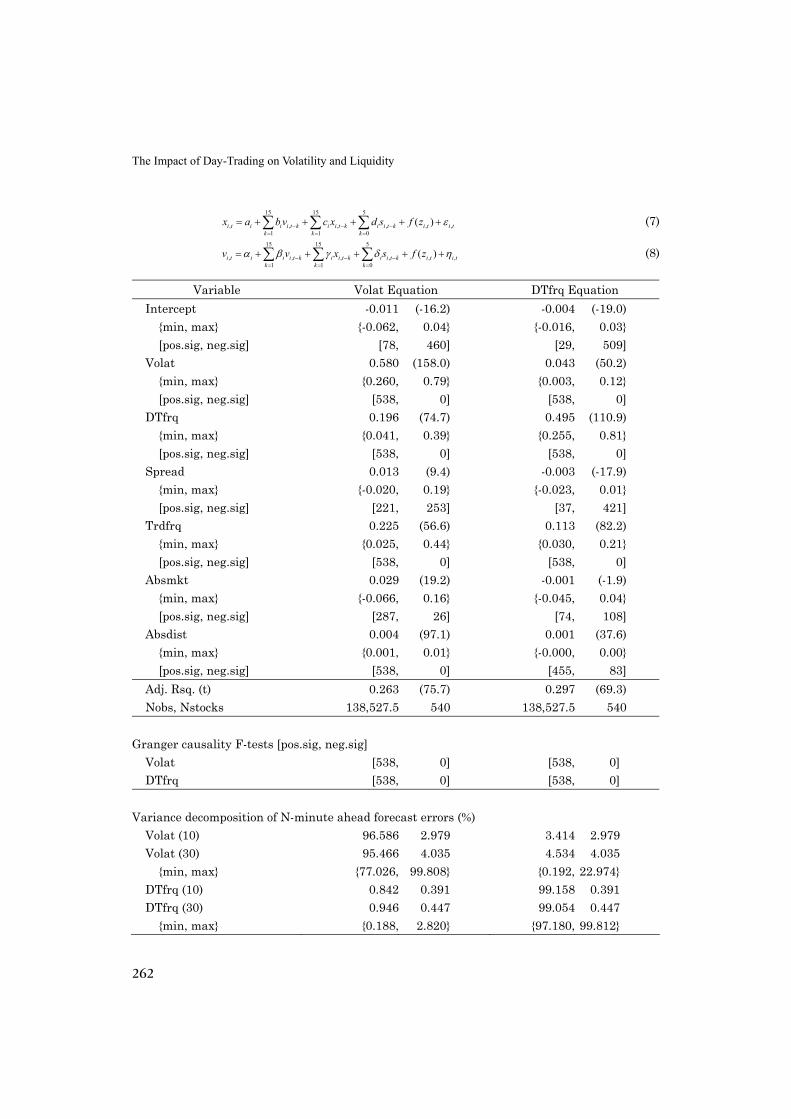
Table 4 presents the regression results for the VAR model of day-trading activity and volatility. The estimation results show that both day-trading activity and volatil-ity variables tend to strongly persist for all stocks in the sample. For example, the sum of the coefficients of the lagged DTfrq in the DTfrq equation is 0.495, and that of the lagged Volat in the Volat equation is 0.580, both of which are positively signifi-
15) We follow the VAR estimation procedures described in Hamilton (1994, Ch. 11). For the asymptotic
distributions of the parameters, see Proposition 11.2 in Hamilton (1994).

Asia-Pacific Journal of Financial Studies (2009) v38 n2
261
cant for 538 stocks out of 540.16) The forecasting error variance decomposition also shows that each of DTfrq and Volat variables explains about 95%-99% of its own fore-cast errors over 30-minute-ahead intervals. The impulse response analysis in Figure 4 suggests that the impact of a one standard deviation shock of DTfrq on future DTfrq lasts about 54.5 minutes, and that of a one standard deviation shock of Volat on future Volat lasts about 82.5 minutes, where these minutes are the time to the first insignificant impulse response at the 1% level. The persistence of return volatil-ity is consistent with the well-known fact that return volatility is positively autocor-related. The persisting pattern in day-trading activity also suggests that day-traders may use similar trading strategies.
It is evident that there are feedback effects between return volatility and day-trading activity. Past return volatility affects future day-trading activity positively for 538 stocks. Figure 4 shows that the impact of a one standard deviation shock of Volat on future DTfrq is high for the first three minutes but decreases gradually until it becomes statistically insignificant after 61.5 minutes. However, Volat explains only
Table 4. Bivariate VARs of day-trading activity and volatility
We estimate the following bivariate VAR system for each of 540 stocks to examine intraday relations between day-trading activities (DTfrq) and volatility (Volat), and report the means of the estimated coefficients (or the sum of the estimates when lag variables are used) across stocks, their t-statistics in parentheses, minimum/maximum values in braces, and the num-bers of stocks with positively or negatively significant coefficient estimates at the 1% level in square brackets. Nobs is the average number of one-minute observations across stocks, and Nstocks is the number of stocks. Also reported is the number of stocks with positively or nega-tively significant F-statistics from the Granger causality test for the null hypothesis that a block of lags of a dependent variable are jointly zeros. For the forecasting error variance de-composition, we assume that the volatility variable is exogenous and report the mean and standard deviation of the variation explained by each of the equations. Control variables as well as main variables are explained in Table 3. The explanatory variables of VAR system in-clude 15 lags for dependent variables, and contemporaneous and 5 lags for control variables except for hour-dummies and Absdist. The estimates for hour-dummies (DH2-DH6) are not reported. If the value of any continuous variable is greater than the 99.9 percentile, it is set to the value of the 99.9 percentile. In the following equations, ,i tx denotes the day-trading variable (DTfrq), ,i tv the volatility variable (Volat), ,i ts the liquidity variable (Spread), and ,( )i tf z other control variables.
16) We also estimate the pooled regression model as in Battalio, Hatch, and Jennings (1997), and find that the
results are qualitatively the same in terms of the magnitude and sign of the estimated coefficients, except for the significance of the t-statistics or F-statistics which becomes far stronger due to the large increase in the number of observations by about 540 times. This additional estimation result further supports the ro-bustness of our results with the bivariate VAR models.
The Impact of Day-Trading on Volatility and Liquidity
262
15 15 5
, , , , , ,1 1 0
( )i t i i i t k i i t k i i t k i t i tk k k
x a b v c x d s f z ε− − −= = =
= + + + + +∑ ∑ ∑ (7) 15 15 5
, , , , , ,1 1 0
( )i t i i i t k i i t k i i t k i t i tk k k
v v x s f zα β γ δ η− − −= = =
= + + + + +∑ ∑ ∑ (8)
Variable Volat Equation DTfrq Equation Intercept -0.011 (-16.2) -0.004 (-19.0)
{min, max} {-0.062, 0.04} {-0.016, 0.03} [pos.sig, neg.sig] [78, 460] [29, 509]
Volat 0.580 (158.0) 0.043 (50.2) {min, max} {0.260, 0.79} {0.003, 0.12} [pos.sig, neg.sig] [538, 0] [538, 0]
DTfrq 0.196 (74.7) 0.495 (110.9) {min, max} {0.041, 0.39} {0.255, 0.81} [pos.sig, neg.sig] [538, 0] [538, 0]
Spread 0.013 (9.4) -0.003 (-17.9) {min, max} {-0.020, 0.19} {-0.023, 0.01} [pos.sig, neg.sig] [221, 253] [37, 421]
Trdfrq 0.225 (56.6) 0.113 (82.2) {min, max} {0.025, 0.44} {0.030, 0.21} [pos.sig, neg.sig] [538, 0] [538, 0]
Absmkt 0.029 (19.2) -0.001 (-1.9) {min, max} {-0.066, 0.16} {-0.045, 0.04} [pos.sig, neg.sig] [287, 26] [74, 108]
Absdist 0.004 (97.1) 0.001 (37.6) {min, max} {0.001, 0.01} {-0.000, 0.00} [pos.sig, neg.sig] [538, 0] [455, 83]
Adj. Rsq. (t) 0.263 (75.7) 0.297 (69.3) Nobs, Nstocks 138,527.5 540 138,527.5 540
Granger causality F-tests [pos.sig, neg.sig]
Volat [538, 0] [538, 0] DTfrq [538, 0] [538, 0]
Variance decomposition of N-minute ahead forecast errors (%)
Volat (10) 96.586 2.979 3.414 2.979 Volat (30) 95.466 4.035 4.534 4.035
{min, max} {77.026, 99.808} {0.192, 22.974} DTfrq (10) 0.842 0.391 99.158 0.391 DTfrq (30) 0.946 0.447 99.054 0.447
{min, max} {0.188, 2.820} {97.180, 99.812}
Asia-Pacific Journal of Financial Studies (2009) v38 n2
263
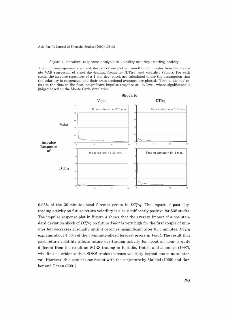
Figure 4. Impulse-response analysis of volatility and day-trading activity
The impulse-responses of a 1 std. dev. shock are plotted from 0 to 30 minutes from the bivari-ate VAR regression of strict day-trading frequency (DTfrq) and volatility (Volat). For each stock, the impulse-responses of a 1 std. dev. shock are calculated under the assumption that the volatility is exogenous, and their cross-sectional averages are plotted. ‘Time to die-out’ re-fers to the time to the first insignificant impulse-response at 1% level, where significance is judged based on the Monte Carlo simulation.
Shock to Volat DTfrq
Volat
0.0
0.2
0.4
0.6
0.8
1.0
0 10 20 30
Time to die-out = 82.5 min.
0.0
0.2
0.4
0.6
0.8
1.0
0 10 20 30
Time to die-out = 61.5 min.
Impulse
Response of
DTfrq
0.0
0.2
0.4
0.6
0.8
1.0
0 10 20 30
Time to die-out = 61.5 min.
0.0
0.2
0.4
0.6
0.8
1.0
0 10 20 30
Time to die-out = 54.5 min.
0.95% of the 30-minute-ahead forecast errors in DTfrq. The impact of past day-trading activity on future return volatility is also significantly positive for 538 stocks. The impulse response plot in Figure 4 shows that the average impact of a one stan-dard deviation shock of DTfrq on future Volat is very high for the first couple of min-utes but decreases gradually until it becomes insignificant after 61.5 minutes. DTfrq explains about 4.53% of the 30-minute-ahead forecast errors in Volat. The result that past return volatility affects future day-trading activity for about an hour is quite different from the result on SOES trading in Battalio, Hatch, and Jennings (1997), who find no evidence that SOES trades increase volatility beyond one-minute inter-val. However, this result is consistent with the conjecture by Malkiel (1999) and Bar-ber and Odean (2001).

The Impact of Day-Trading on Volatility and Liquidity
264
There is little surprise in the coefficient estimates of the control variables. Trading activity (Trdfrq), both contemporaneous and five lagged, has positive impacts on both return volatility and day-trading activity. KOSPI return volatility, both contempora-neous and five lagged, tends to increase return volatility. However, its impact on day-trading activity is unclear, indicating that day-traders are little concerned about the general market movement. Regarding the coefficient estimates of the hour dummy variables (not reported in a table), return volatility shows a familiar J-shape intraday pattern as documented in numerous studies, and day-trading activity shows an in-verted U-shape.
We also examine interactions between day-trading activity and liquidity in a simi-lar VAR framework. Table 5 shows that past day-trading activity reduces future bid-ask spreads for many stocks. The sum of the coefficient estimates of lagged DTfrq variables in the Spread equation is -0.116 on average, and is significantly negative for 436 stocks among 540 sample stocks. The impulse response analysis depicted in Figure 5 shows that the impact of a one standard deviation day-trading shock on bid-ask spreads last for a long time (about 163.8 minutes). In addition, the forecasting error variance decomposition shows that DTfrq explains about 11% of the 30-minute-ahead forecast errors in Spread. The evidence that day-trading activity enhances li-quidity is consistent with Barber and Odean’s (2001) argument that day-trading ac-tivity provides the market with instant liquidity.
Table 5. Bivariate VARs of day-trading activity and liquidity
We estimate the following bivariate VAR system for each of 540 stocks to examine intraday relations between day-trading activities (DTfrq) and liquidity (Spread), and report the means of the estimated coefficients (or the sum of the estimates when lag variables are used) across stocks, their t-statistics in parentheses, minimum/maximum values in braces, and the num-bers of stocks with positively or negatively significant coefficient estimates at the 1% level in square brackets. Nobs is the average number of one-minute observations across stocks, and Nstocks is the number of stocks. Also reported is the number of stocks with positively or nega-tively significant F-statistics from the Granger causality test for the null hypothesis that a block of lags of a dependent variable are jointly zeros. For the forecasting error variance de-composition, we assume that the liquidity variable is exogenous and report the mean and standard deviation of the variation explained by each of the equations. Control variables as well as main variables are explained in Table 3. The explanatory variables of VAR system in-clude 15 lags for dependent variables, and contemporaneous and 5 lags for control variables except for hour-dummies and Absdist. The estimates for hour-dummies (DH2-DH6) are not reported. If the value of any continuous variable is greater than the 99.9 percentile, it is set to the value of the 99.9 percentile. In the following equations, ,i tx denotes the day-trading variable (DTfrq), ,i ts the liquidity variable (Spread), ,i tv the volatility variable (Volat), and ,( )i tf z other con-trol variables.

Asia-Pacific Journal of Financial Studies (2009) v38 n2
265
15 15 5
, , , , , ,1 1 0
( )i t i i i t k i i t k i i t k i t i tk k k
x a b s c x d v f z ε− − −= = =
= + + + + +∑ ∑ ∑ (7)’
15 15 5
, , , , , ,1 1 0
( )i t i i i t k i i t k i i t k i t i tk k k
s s x v f zα β γ δ η− − −= = =
= + + + + +∑ ∑ ∑ (8)’
Variables Spread Equation DTfrq Equation Intercept 0.022 (31.2) -0.004 (-20.9) {min, max} {-0.026, 0.09} {-0.018, 0.02} [pos.sig, neg.sig] [429, 109] [21, 517]
Spread 0.920 (388.5) -0.004 (-16.0) {min, max} {0.694, 1.00} {-0.035, 0.01} [pos.sig, neg.sig] [538, 0] [40, 410]
DTfrq -0.116 (-32.6) 0.483 (112.7) {min, max} {-0.347, 0.11} {0.254, 0.79} [pos.sig, neg.sig] [11, 436] [538, 0]
Volat 0.029 (17.8) 0.066 (62.9) {min, max} {-0.057, 0.14} {0.015, 0.18} [pos.sig, neg.sig] [315, 54] [538, 0]
Trdfrq 0.209 (71.6) 0.105 (79.7) {min, max} {0.036, 0.39} {0.028, 0.20} [pos.sig, neg.sig] [538, 0] [538, 0]
Absmkt 0.007 (5.2) -0.003 (-5.5) {min, max} {-0.088, 0.10} {-0.046, 0.04} [pos.sig, neg.sig] [123, 48] [66, 131]
Absdist 0.000 (10.7) 0.000 (25.6) {min, max} {-0.002, 0.00} {-0.001, 0.00} [pos.sig, neg.sig] [118, 420] [354, 184]
Adj. Rsq. (t) 0.752 (113.2) 0.305 (72.1) Nobs, Nstocks 138,527.5 540 138,527.5 540
Granger causality F-tests [pos.sig, neg.sig]
Spread [538, 0] [72, 461] DTfrq [8, 339] [538, 0]
Variance decomposition of N-minute ahead forecast errors (%)
Spread (10) 93.062 2.636 6.938 2.636 Spread (30) 89.037 4.350 10.963 4.350 {min, max} {67.791, 98.329} {1.671,32.209}
DTfrq (10) 0.065 0.081 99.935 0.081 DTfrq (30) 0.186 0.203 99.814 0.203 {min, max} {0.003, 1.287} {98.713,99.997}
The Impact of Day-Trading on Volatility and Liquidity
266
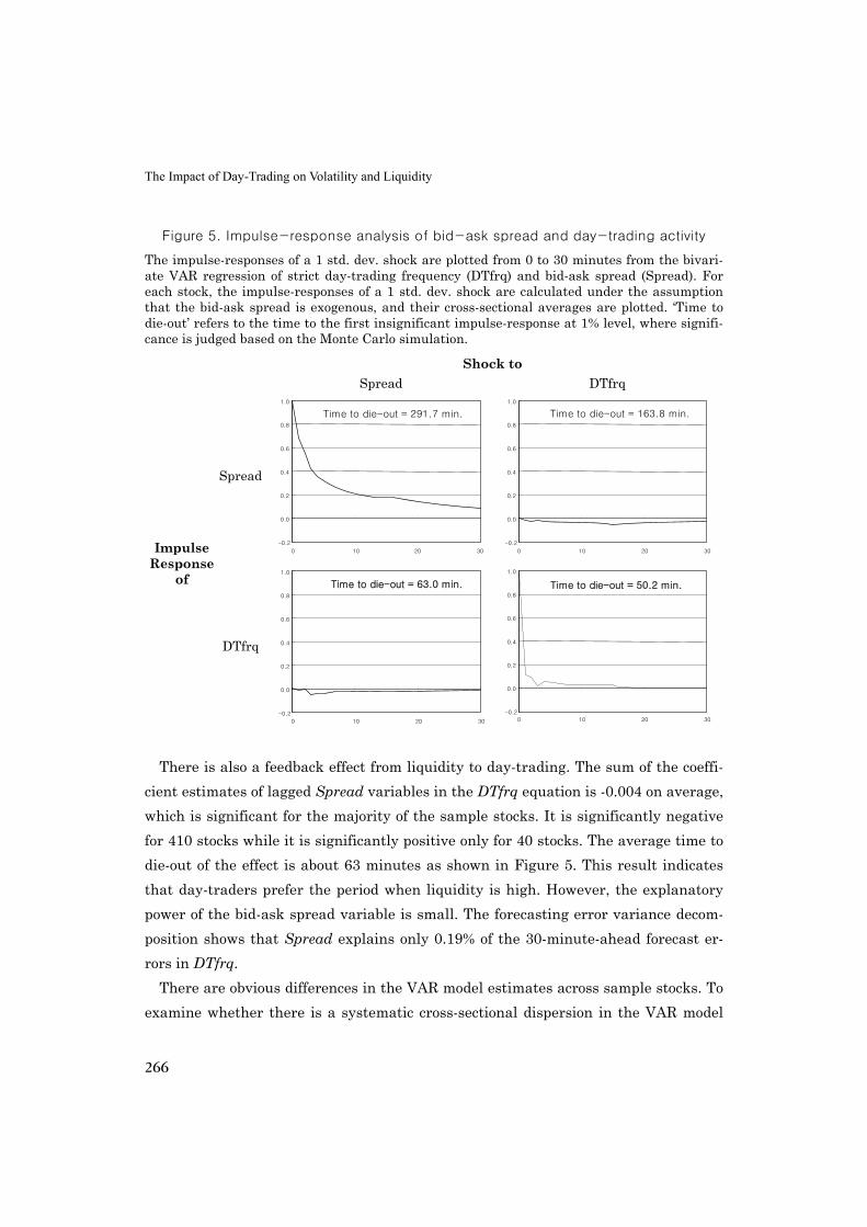
Figure 5. Impulse-response analysis of bid-ask spread and day-trading activity
The impulse-responses of a 1 std. dev. shock are plotted from 0 to 30 minutes from the bivari-ate VAR regression of strict day-trading frequency (DTfrq) and bid-ask spread (Spread). For each stock, the impulse-responses of a 1 std. dev. shock are calculated under the assumption that the bid-ask spread is exogenous, and their cross-sectional averages are plotted. ‘Time to die-out’ refers to the time to the first insignificant impulse-response at 1% level, where signifi-cance is judged based on the Monte Carlo simulation.
Shock to Spread DTfrq
Spread
-0.2
0.0
0.2
0.4
0.6
0.8
1.0
0 10 20 30
Time to die-out = 291.7 min.
-0.2
0.0
0.2
0.4
0.6
0.8
1.0
0 10 20 30
Time to die-out = 163.8 min.
Impulse Response
of
DTfrq
-0.2
0.0
0.2
0.4
0.6
0.8
1.0
0 10 20 30
Time to die-out = 63.0 min.
-0.2
0.0
0.2
0.4
0.6
0.8
1.0
0 10 20 30
Time to die-out = 50.2 min.
There is also a feedback effect from liquidity to day-trading. The sum of the coeffi-
cient estimates of lagged Spread variables in the DTfrq equation is -0.004 on average, which is significant for the majority of the sample stocks. It is significantly negative for 410 stocks while it is significantly positive only for 40 stocks. The average time to die-out of the effect is about 63 minutes as shown in Figure 5. This result indicates that day-traders prefer the period when liquidity is high. However, the explanatory power of the bid-ask spread variable is small. The forecasting error variance decom-position shows that Spread explains only 0.19% of the 30-minute-ahead forecast er-rors in DTfrq.
There are obvious differences in the VAR model estimates across sample stocks. To examine whether there is a systematic cross-sectional dispersion in the VAR model
Asia-Pacific Journal of Financial Studies (2009) v38 n2
267
estimates, we divide the entire sample into various deciles based on day-trading fre-quency, price level, trading value, and volatility. However, we find little cross-sec-tional variation in the VAR model estimates across deciles for each partitioning vari-able. Thus, we do not report the results in a separate table.
5. The impact of day-trading imbalance on intraday returns
In the previous section, we have seen that day-trading activity raises intraday re-turn volatility for about an hour. However, this result does not necessarily imply that day-trading activity destabilizes stock prices. We examine this question further in this section with day-trading variables that take into account net-buy or net-sell di-rection of trades (i.e., day-trading order imbalance, as defined previously) in a bivari-ate VAR system.17) Therefore, the VAR system here differs from those of the previous section in that we now use ‘signed’ variables for both dependent variables and that we examine the direction of stock price movements before and after day-trading ac-tivity. This analysis also provides us with deeper understanding of the nature of day-traders’ trading strategies. That is, it enables us to test whether day-traders follow momentum or contrarian strategies by allowing us to observe minute-by-minute re-turns behavior before and after day-trading activity.
5.1 The VAR framework
Our bivariate VAR system has a day-trading order imbalance measure (IDTfrq or IDTvol) and log-return as the dependent variables. The log-returns are based on bid-ask midpoints observed at the end of two adjacent intervals to minimize the impact of bid-ask bounce. The explanatory variables include 15 lags of the two dependent vari-ables as before and the following control variables. (1) Imbfrq and Imbvol: These variables are price-setting order imbalances in each
one-minute interval normalized by either the total frequency of trades on the day (for Imbfrq) or the total share volume traded on the day (for Imbvol). The price-setting order imbalance in a one-minute interval is the difference between the
17) We have also examined this question in an event study framework with large day-trading order imbal-
ances similar to Choe, Kho, and Stulz (1999), and obtained the same results as in the VAR framework.
The Impact of Day-Trading on Volatility and Liquidity
268
price-setting buy and sell volume, where the price-setting buy volume refers to ei-ther the number of buyer-initiated transactions (for Imbfrq) or the share volume initiated by buyers (for Imbvol), and the price-setting sell volume is similarly de-fined. Since our data contain the order sequence number for each side of a trade, we are able to classify each trade as being a buyer- or seller-initiated trade with-out relying on a special algorithm proposed by Lee and Ready (1991). That is, if the buyer (seller) of a trade placed his order later than the seller (buyer), the trade is classified as buyer-initiated (seller-initiated). The two variables control for the normal impact of price-setting order imbalance on stock returns and day-trading imbalance. Both contemporaneous and 5 lagged variables are included.
(2) Mkt: This is the one-minute log-return on the nearest-term KOSPI 200 index fu-tures. It controls for the influence of the market-wide factor on stock returns and day-trading imbalance. Both contemporaneous and 5 lagged variables are included.
(3) DH1, …, DH6: These hour dummies are used to control for the well-known time-
of-day effect in returns and the intraday pattern of day-trading imbalance. As ex-plained before, we do not include the dummy for the first hour (DH1) to avoid the linear dependence problem.
(4) Dist: This variable is the log-return calculated from the closing price on the previ-ous day to the trading price at the end of the previous one-minute interval. Thus, it is essentially a signed distance measure that controls for the impact of the price limit hit on stock returns and day-trading imbalance.
Table 6 presents summary statistics of the variables used in the VAR models.
Clearly, there are some observations with exceptionally high or low values for most of the variables. To avoid the impact of those outliers on the VAR estimation results, we set values of any continuous variable greater than the 99.95 percentile to the value of the 99.95 percentile and set those smaller than 0.05 percentile to the value of the 0.05 percentile.
As before, we estimate the bivariate VAR models for each stock using the variables measured in one-minute intervals. For the Granger causality tests, impulse response analyses, and N-minute ahead forecasting error decomposition, we use the techniques identical to those used in Tables 4 and 5.

Asia-Pacific Journal of Financial Studies (2009) v38 n2
269
Table 6. Summary statistics of the variables used in VAR models of day-trading order
imbalance and returns
If an account buys and sells an equal number of shares for a stock on the same day, all of the buy and sell trades are classified as strict day-trading. If an account both buys and sells any numbers of shares for a stock on the same day (buy and sell volumes need not be equal), all of the buy and sell trades are classified as lenient day-trading. We use one-minute interval to measure all variables used in the VAR models. For each variable reported below, we calculate the mean, standard deviations, and various percentile statistics across all one-minute intervals for each stock, and report cross-sectional averages of these statistics except for the maximum and minimum statistics, which are the maximum and minimum values across stocks. For each one-minute interval, IDTfrq (%) is the difference between the buy and sell frequencies divided by the number of trades occurring during the day, and IDTvol (%) is the difference between the buy and sell share volume divided by the number of shares traded on the day. Ret (%) is the one-minute log return based on bid-ask middle points. Imbfrq (%) is the price-setting order imbalance normalized by the number of total trades on the day, and Imbvol (%) is the price-setting order imbalance normalized by the number of shares traded on the day. Mkt (%) is the one-minute log return on the nearest-term KOSPI 200 futures contract. Dist (%) is the log re-turn calculated from the closing price on the previous day to the trading price at the end of the previous one-minute interval.
Strict day-trading Lenient day-trading
IDTfrq IDTvol IDTfrq IDTvol Ret Imbfrq Imbvol Mkt Dist
Mean 0.001 0.002 0.006 0.005 0.000 -0.033 -0.044 0.000 0.195 Std.dev. 0.241 0.284 0.335 0.432 0.344 0.730 1.020 0.125 4.029 Max 100.000 100.000 100.000 100.000 24.147 100.000 100.000 1.439 13.976 99.95% 2.994 3.689 3.958 5.289 3.019 7.189 10.574 0.668 13.943 75% 0.002 0.001 0.006 0.003 0.007 0.017 0.012 0.072 2.148 50% 0.000 0.000 0.000 0.000 0.000 0.000 0.000 0.000 0.033 25% -0.002 -0.001 -0.004 -0.002 -0.008 -0.042 -0.029 -0.070 -2.097 0.05% -2.573 -3.193 -3.399 -4.765 -2.888 -7.781 -12.815 -0.701 -15.052 Min -100.000 -100.000 -100.000 -100.000 -22.156 -100.000 -100.000 -6.744 -16.252
5.2 VAR regression results
Table 7 presents the regression results for the VAR model of day-trading order im-balance and stock return. The return equation reveals a strong short-term mean re-verting behavior of minute-by-minute returns. The sum of the estimated coefficients of past returns is -0.436 on average, which is significant for all sample stocks. Consis-tent with negative autocorrelations in minute-by-minute returns, Figure 6 shows that the impulse response to a one standard deviation shock of Ret is oscillating for the first few minutes. Unlike stock returns, day-trading order imbalance is strongly
The Impact of Day-Trading on Volatility and Liquidity
270
persistent. In the day-trading order imbalance equation, the sum of the estimated coefficients of past IDTfrq variables is 0.312 on average, which is significant for all stocks. The persistence in IDTfrq suggests that day-traders may act similarly upon the common signal.
Interestingly, it appears that day-traders seem to use very short-term contrarian strategies rather than momentum strategies. The sum of the estimated coefficients of past returns in the day-trading order imbalance equation is -0.047 on average. This sum is significant for 470 stocks among 540 sample stocks, while being significantly positive only for 3 stocks. However, the magnitude of the impulse response of a one standard deviation return shock to the day-trading order imbalance shown in Figure 6 is quite small, and the time to die-out of the impulse response is short in about 17 minutes. Further, the forecasting error variance decomposition shows that stock re-turns explain only 0.19% of the 30-minute-ahead forecast errors in IDTfrq.
It appears that past day-trading order imbalance affects future returns positively. The sum of the coefficient estimates is significantly positive (0.139, on average) for 537 stocks. This result, together with the contrarian strategy explained above, is con-sistent with a cyclical behavior of day-traders who look for short-term price cycles and concentrate their buy or sell trades at the bottom or peak of the price cycles, re-spectively. However, the impulse responses drawn in Figure 6 are very small in gen-eral and become negligible in magnitude in about 2 minutes, although they remain statistically significant for about 15 minutes.
Table 7. Bivariate VARs of day-trading order imbalance and stock return
We estimate the following bivariate VAR system for each of 540 stocks to examine intraday relations between day-trading order imbalance (IDTfrq) and stock returns (Ret), and report the means of the estimated coefficients (or the sum of the estimates when lag variables are used) across stocks, their t-statistics in parentheses, minimum/maximum values in braces, and the numbers of stocks with positively or negatively significant coefficient estimates at the 1% level in square brackets. Nobs is the average number of one-minute observations across stocks, and Nstocks is the number of stocks. Also reported is the number of stocks with positively or nega-tively significant F-statistics from the Granger causality test for the null hypothesis that a block of lags of a dependent variable are jointly zeros. For the forecasting error variance de-composition, we assume that the return variable is exogenous and report the mean and stan-dard deviation of the variation explained by each of the equations. Control variables as well as main variables are explained in Table 6. The explanatory variables of VAR system include 15 lags for dependent variables, and contemporaneous and 5 lags for control variables except for hour-dummies and Dist. The estimates for hour-dummies (DH2-DH6) are not reported. If the value of any continuous variable is greater than the 99.9 percentile, it is set to the value of the 99.9 percentile. In the following equations, ,i tx denotes the day-trading variable (IDTfrq), ,i tr the return (Ret), and ,( )i tf z other control variables.

Asia-Pacific Journal of Financial Studies (2009) v38 n2
271
15 15
, , , , ,1 1
( )i t i i i t k i i t k i t i tk k
x a b r c x f z ε− −= =
= + + + +∑ ∑ (7)’ 15 15
, , , , ,1 1
( )i t i i i t k i i t k i t i tk k
r r x f zα β γ η− −= =
= + + + +∑ ∑ (8)’
Ret Equation IDTfrq Equation Intercept 0.000 (2.5) 0.018 (75.4)
{min, max} {-0.011, 0.01} {0.003, 0.03} [pos.sig, neg.sig] [44, 496] [540, 0]
Ret -0.436 (-132.5) -0.047 (-37.5) {min, max} {-0.697, -0.17} {-0.138, 0.04} [pos.sig, neg.sig] [0, 540] [3, 470]
IDTfrq 0.139 (57.5) 0.312 (116.0) {min, max} {-0.006, 0.36} {0.153, 0.53} [pos.sig, neg.sig] [537, 0] [540, 0]
Imbfrq 0.270 (88.7) 0.020 (18.0) {min, max} {0.066, 0.50} {-0.037, 0.11} [pos.sig, neg.sig] [540, 0] [373, 110]
Mkt 0.209 (29.6) 0.039 (34.2) {min, max} {-0.013, 0.86} {-0.035, 0.15} [pos.sig, neg.sig] [520, 0] [438, 3]
Dist -0.002 (-75.1) -0.001 (-38.7) {min, max} {-0.003, -0.00} {-0.002, 0.00} [pos.sig, neg.sig] [0, 540] [9, 531]
Adj Rsq (t) 0.207 (275.7) 0.053 (25.4) Nobs, Nstocks 138,534.6 540 138,534.6 540
Granger causality F-tests [pos.sig, neg.sig]
Ret [0, 540] [3, 378] IDTfrq [526, 0] [540, 0]
Variance decomposition of N-minute ahead forecast errors (%)
Ret (10) 99.652 0.217 0.348 0.217 Ret (30) 99.622 0.246 0.378 0.246
{min, max} {98.668, 99.950} {0.050, 1.332} IDTfrq (10) 0.181 0.166 99.819 0.166 IDTfrq (30) 0.191 0.167 99.809 0.167
{min, max} {0.006, 1.408} {98.592,99.994}
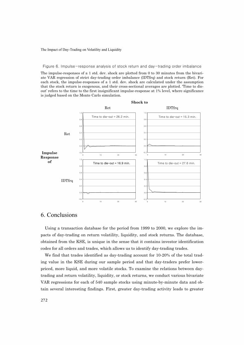
The Impact of Day-Trading on Volatility and Liquidity
272
Figure 6. Impulse-response analysis of stock return and day-trading order imbalance
The impulse-responses of a 1 std. dev. shock are plotted from 0 to 30 minutes from the bivari-ate VAR regression of strict day-trading order imbalance (IDTfrq) and stock return (Ret). For each stock, the impulse-responses of a 1 std. dev. shock are calculated under the assumption that the stock return is exogenous, and their cross-sectional averages are plotted. ‘Time to die-out’ refers to the time to the first insignificant impulse-response at 1% level, where significance is judged based on the Monte Carlo simulation.
Shock to Ret IDTfrq
Ret
-0.2
0.0
0.2
0.4
0.6
0.8
1.0
0 10 20 30
Time to die-out = 26.2 min.
-0.2
0.0
0.2
0.4
0.6
0.8
1.0
0 10 20 30
Time to die-out = 15.3 min.
Impulse
Response of
IDTfrq
-0.2
0.0
0.2
0.4
0.6
0.8
1.0
0 10 20 30
Time to die-out = 16.9 min.
-0.2
0.0
0.2
0.4
0.6
0.8
1.0
0 10 20 30
Time to die-out = 27.6 min.
6. Conclusions
Using a transaction database for the period from 1999 to 2000, we explore the im-pacts of day-trading on return volatility, liquidity, and stock returns. The database, obtained from the KSE, is unique in the sense that it contains investor identification codes for all orders and trades, which allows us to identify day-trading trades.
We find that trades identified as day-trading account for 10-20% of the total trad-ing value in the KSE during our sample period and that day-traders prefer lower-priced, more liquid, and more volatile stocks. To examine the relations between day-trading and return volatility, liquidity, or stock returns, we conduct various bivariate VAR regressions for each of 540 sample stocks using minute-by-minute data and ob-tain several interesting findings. First, greater day-trading activity leads to greater

Asia-Pacific Journal of Financial Studies (2009) v38 n2
273
return volatility at the intraday level. The impulse responses of return volatility to a day-trading shock dissipate gradually for about an hour. There is also a positive feedback effect from return volatility to day-trading activity. Second, greater day-trading activity leads to a lower bid-ask spread, suggesting that day-trading plays a role in enhancing market liquidity. There is also a negative feedback effect from bid-ask spreads to day-trading activity, supporting the evidence of day-traders’ prefer-ence for liquid stocks. Finally, we find strong evidence that day-traders use short-term contrarian strategies rather than momentum strategies, and that past day-trading order imbalance positively affects future stock returns. This result is consis-tent with a cyclical behavior of day-traders who concentrate their buy or sell trades at the bottom or peak of the short-term price cycles, respectively. However, the impulse response analysis as well as the forecasting error variance decomposition analysis suggests that the results are rather weak.

The Impact of Day-Trading on Volatility and Liquidity
274
References
Barber, Brad M. and Terrance Odean, 2000, Trading is Hazardous to Your Wealth: The Common Stock Investment Performance of Individual Investors, Journal of Finance 55 (2), pp. 773-806.
Barber, Brad M. and Terrance Odean, 2001, The Internet and the Investor, Journal of Economic Perspectives 15 (1), pp. 41-54.
Barber, Brad M. and Terrance Odean, 2002, Online Investors: Do the Slow Die First?, Review of Financial Studies 15 (2), pp. 455-487.
Barber, Brad M., Y.-T. Lee, Y.-J. Liu, and Terrance Odean, 2004, Do Individual Day Traders Make Money? Evidence from Taiwan, Working Paper, University of Cali-fornia, Berkeley.
Battalio, Robert H., Brian Hatch, and Robert Jennings, 1997, SOES Trading and Market Volatility, Journal of Financial and Quantitative Analysis 32 (2), pp. 225-238.
Choe, Hyuk, Bong-Chan Kho, and René M. Stulz, 1999, Do Foreign Investors Desta-bilize Stock Markets? The Korean Experience in 1997, Journal of Financial Eco-nomics 54 (2), pp. 227-264.
Choi, James J., David Laibson, and Andrew Metrick, 2002, How Does the Internet Affect Trading? Evidence from Investor Behavior in 401(k) Plans, Journal of Fi-nancial Economics 64 (3), pp. 397-421.
Chun, Chun-Ok, 2001, The Impact of Day-Trading and Online Trading, Securities, Korea Securities Dealers’ Association, 107, pp. 50-72.
ETA, 1999, Statement of Electronic Traders Association for Hearing before the Per-manent Subcommittee on Investigations Committee on Governmental Affairs, Uni-ted States Senate, Electronic Traders Association.
Hamilton, 1994, Time Series Analysis, Princeton University Press. Harris, Jeffrey H. and Paul H. Schultz, 1997, The Importance of Firm Quotes and
Rapid Executions: Evidence from the January 1994 SOES Rules Change, Journal of Financial Economics 45 (1), pp. 135-166.
Harris, Jeffrey H. and Paul H. Schultz, 1998, The Trading Profits of SOES Bandits, Journal of Financial Economics 50 (1), pp. 39-62.
Lee, Charles M. C. and Mark J. Ready, 1991, Inferring Trade Direction from Intraday Data, Journal of Finance 46 (2), pp. 733-746.

Asia-Pacific Journal of Financial Studies (2009) v38 n2
275
Lee, Eunjung, Kyung-Suh Park, and Hasung Jang, How Profitable is Day Trading? A Study on Day-Trading in Korean Stock Market, Asia-Pacific Journal of Financial Studies 36 (3), pp. 351-385.
Linnainmaa, Juhani, 2005, The Individual Day Trader, Working Paper, The Ander-son School at UCLA.
Lutkepohl, H., 1991, Introduction to Multiple Time Series Analysis, Springer-Verlag, Berlin.
Malkiel, 1999, Day Trading and Its Dangers, The Wall Street Journal. NASAA, 1999, Report of the Day Trading Project Group, North American Securities
Administrators Association. Odean, Terrance, 1999, Do Investors Trade Too Much?, American Economic Review
89 (5), pp. 1279-1298. Pesaran, H. Hashem and Yongcheol Shin, 1998, Generalized impulse response analy-
sis in linear multivariate models, Economics Letters 58, pp. 17-29. SEC, 2000, Special Study: Report of Examinations of Day-Trading Broker-Dealers,
US Securities and Exchange Commission. Song, Chi-Seung, 2003, Day Trading and Price Volatility: Observation of the Korea
Stock Exchange, Asia-Pacific Journal of Financial Studies 32 (3), pp. 45-84. Statman, Meir, Steven Thorley, and Keith Vorkink, 2006, Investor Overconfidence
and Trading Volume, Review of Financial Studies 19 (4), pp. 1531-1565. World Federation of Exchanges, 1999, Annual Statistics, International Federation of
Stock Exchange, http://www.world-exchanges.org/.
