idiosyncratic volatility and the cross section of expected...
TRANSCRIPT

JOURNAL OF FINANCIAL AND QUANTITATIVE ANALYSIS Vol. 43, No. 1, March 2008, pp. 29-58COPYRIGHT 2008. MICHAEL G. FOSTER SCHOOL OF BUSINESS. UNIVERSITY OF WASHINGTON. SEATTLE. WA 98195
Idiosyncratic Volatility and the Cross Section ofExpected Returns
Turan G. Bali and Nusret Cakici*
Abstract
This paper examines the cross-sectional relation between idiosyncratic volatility and ex-pected stock returns. The results indicate that i) the data frequency used to estimate id-iosyncratic volatility, ii) the weighting scheme used to compute average portfolio returns,iii) the breakpoints utilized to sort stocks into quintile portfolios, and iv) using a screen forsize, price, and liquidity play critical roles in determining the existence and significance ofa relation between idiosyncratic risk and the cross section of expected returns. Portfolio-level analyses based on two different measures of idiosyncratic volatility (estimated usingdaily and monthly data), three weighting schemes (value-weighted, equal-weighted, in-verse volatility-weighted), three breakpoints (CRSP, NYSE, equal market share), and twodifferent samples (NYSE/AMEX/NASDAQ and NYSE) indicate that no robustly signifi-cant relation exists between idiosyncratic volatility and expected returns.
I. Introduction
The capital asset pricing model (CAPM) of Sharpe (1964), Lintner (1965a),and Black (1972) implies the mean-variance efficiency of the market portfolio inthe sense of Markowitz (1959). The primary implication of the Sharpe-Lintner-Black (SLB) model is that there exists a positive linear relation between expectedreturns on securities and their market betas, and variables other than beta shouldnot capture the cross-sectional variation in expected returns. However, there issome theoretical evidence that idiosyncratic volatility is positively related to the
*Bali, [email protected]. Department of Economics and Finance, Baruch College, Zick-lin School of Business, City University of New York, One Bernard Baruch Way, Box 10-225, NewYork, NY 10010 and College of Administrative Sciences and Economics, Koc LIniversity, RumeliFeneri Yolu, Istanbul, Turkey 34450; Cakici, [email protected]. Department of Economics and Fi-nance, School of Global Management, Arizona State University, PO Box 37100, Phoenix, AZ 85069.We thank Stephen Brown (the editor) and Xiaotong (Vivian) Wang (the referee) for their extremelyhelpful comments and suggestions. We also thank Andrew Ang, Wayne Ferson, Robert Hodrick,Haim Levy, Sheridan Titman, Robert Whitelaw, Yuhang Xing, and Xiaoyan Zhang for their usefulcomments on earlier versions of this paper. We also benefited from discussions with Linda Allen, SrisChatterjee, Ozgur Demirtas, Armen Hovakimian, John Merrick, Lin Peng, Robert Schwartz, DavidWeinbaum, and Liuren Wu on certain theoretical and empirical points. An earlier version of this pa-per was presented at Baruch College, City College, and the Graduate School and University Center ofCily University of New York. Bali gratefully acknowledges the financial support from the PSC-CUNYResearch Foundation of City tJniversity of New York. All errors remain our responsibility.
29
30 Journal of Financial and Quantitative Analysis
cross section of expected returns if investors demand compensation for not be-ing able to diversify firm-specific variance. Levy (1978) theoretically shows thatidiosyncratic risk affects equilibrium asset prices if investors do not hold manyassets in their portfolios. Merton (1987) indicates that if investors cannot hold themarket portfolio they will care about total risk, not simply market risk. There-fore, firms with larger total (or idiosyncratic) variance require higher returns tocompensate for imperfect diversification.'
Supporting the theoretical models, Tinic and West (1986) and Malkiel andXu (1997) provide empirical evidence that portfolios with higher idiosyncraticvolatility have higher average returns. However, they do not present any signifi-cance levels for their idiosyncratic volatility premiums. Lehmann (1990) consid-ers residual variance in the cross-sectional firm-level regressions and also finds astatistically significant, positive coefficient on idiosyncratic volatility over his fullsample period, but he shows that the coefficient on idiosyncratic risk changes signin different econometric specifications.^
More recently, Malkiel and Xu (2002) find a significantly positive relationbetween idiosyncratic risk and the cross section of expected returns at the firmlevel. However, their main findings are not based on a measure of an individualstock's idiosyncratic volatility. Instead, they assign a stock's residual standarddeviation to be the idiosyncratic risk of one of the 200 beta/size portfolios towhich that stock belongs each month. Ang, Hodrick, Xing, and Zhang (2006)(AHXZ hereafter) measure idiosyncratic volatility of individual stocks based onthe three-factor Fama-French (1993) model and then generate portfolios of stockssorted by the individual stocks' idiosyncratic volatility. In contrast to Malkiel andXu (2002), AHXZ (2006) show that stocks with low idiosyncratic risk earn highaverage returns, and the average return differential between quintile portfolios ofthe lowest and highest idiosyncratic risk is about — 1.06% per month. Contrary tothe existing literature, AHXZ (2006) indicate a strong negative relation betweenidiosyncratic volatility and expected stock returns.
Fu (2005) shows that idiosyncratic risk varies substantially over time and in-dicates that the existing literature cannot identify a positive relation because theconditional idiosyncratic volatility in earlier studies does not capture the time-varying property. Using monthly data, Fu provides in-sample estimates of theconditional idiosyncratic variance of stock returns based on the EGARCH modelof Nelson (1991) and finds a significantly positive relation. Also using monthly
'in very early work, Douglas (1969) and Lintner (t965b) find that average stock returns are sig-nificantly related to the estimates of betas and total (or idiosyncratic) variances. However, Mitler andScholes (1972) indicate important statistical problems with these results and suggest that considerablecaution should be exercised when using total or residual risk as an explanatory variable, Fama andMacBeth (1973) introduce a more powerful cross-sectional test and find no idiosyncratic risk effectwhen residual variances and betas are estimated in an earlier period to mitigate the Miller-Scholesproblem,
^Some indirect evidence regarding the role of idiosyncratic risk has been provided in recent years,Bessembinder (1992) finds support for the cross-sectional pricing of idiosyncratic risk in futures mar-kets. King, Sentana, and Wadhwani (1994) provide evidence that idiosyncratic risk is priced and theprice of risk associated with the relevant factors is not the same across countries, Falkenstein (1996)indicates that the equity holdings of mutual fund managers are related to the idiosyncratic volatility ofindividual stocks. Green and Rydqvist (1997) show that Swedish lottery bonds command a premiumfor a risk that is idiosyncratic by construction, Jones and Rhodes-Kropf (2003) find that idiosyncraticrisk is priced in the private equity and venture capital markets even if investors can fully diversify.
Bali and Cakici 31
data, Spiegel and Wang (2005) focus on the out-of-sample predictive power ofidiosyncratic volatility and liquidity, and find that expected stock returns are in-creasing with the level of idiosyncratic risk and decreasing in a stock's liquidity.Their major finding is that while both liquidity and idiosyncratic risk play a majorrole in determining stock returns, the impact of conditional idiosyncratic risk ismuch stronger.
As discussed above, there has been a lively debate on the existence and di-rection of a trade-off between idiosyncratic risk and the cross section of expectedstock returns. Although some studies find a positive relation between idiosyn-cratic volatility and expected returns at the firm or portfolio level, often the cross-sectional relation has been found insignificant, and sometimes even negative.
The purpose of this paper is to clarify the existence and significance of arelation between idiosyncratic risk and expected returns. The paper also shedslight on the methodological differences in previous studies that mainly led theexisting literature to present confiicting evidence. We find strong evidence thati) the data frequency used to calculate idiosyncratic risk, ii) the weighting schemeadopted for generating average portfolio returns, iii) the breakpoints utilized tosort stocks into quintile (or decile) portfolios, and iv) using a screen for size, price,and liquidity play critical roles in determining the presence and significance of across-sectional relation between idiosyncratic risk and expected returns.^
Following AHXZ (2006), we use within-month daily data to calculate id-iosyncratic volatility based on the three-factor Fama-French (1993) model (FF-3)and then generate portfolios of stocks sorted by the estimated idiosyncratic volatil-ity. When we use all NYSE/AMEX/NASDAQ stocks (CRSP breakpoints) to sortthem into quintile portfolios, the value-weighted average return differential be-tween the lowest and highest idiosyncratic volatility portfolios is about -0.93%per month and highly significant for the extended sample period from July 1963-December 2004. This result is similar to the finding of AHXZ (2006): -1.06%per month for the period from July 1963-December 2000.
Instead of comparing the value-weighted returns on quintile portfolios whenwe form the equal-weighted portfolios, we find no evidence of a significantly neg-ative relation between idiosyncratic risk and the cross section of expected returns.More specifically, the equal-weighted average return differential between the low-est and highest idiosyncratic risk portfolios obtained from the same CRSP break-points is a small positive number, 0.02% per month, and statistically insignifi-cant. As an additional modification to the AHXZ (2006) methodology, we weightstocks in quintile portfolios by the inverse of their idiosyncratic volatility ratherthan by their capitalization. This method gives lower weight to those stocks withhigher idiosyncratic risk.'' Similar to our findings from equal-weighted portfolios,the inverse volatility-weighted average return differential between the lowest andhighest idiosyncratic risk portfolios obtained from the same CRSP breakpoints
• In this paper, we do not investigate ttie cross-sectional relation between expected stock returnsand expected idiosyncratic volatilities conditioned on past information or firm-specific variables.Therefore, our results are not comparable to Fu (2005) and Spiegel and Wang (2005) who use aconditional time-varying measure of idiosyncratic volatility.
''As will be discussed later, stocks with high idiosyncratic risk are generally small, illiquid, andlow priced. Hence, the objective of using inverse volatility-weighted portfolios is to give lower weightto the smallest, least liquid, and lowest priced stocks.
32 Journal of Financial and Quantitative Analysis
is a small positive number, 0.08% per month, and statistically insignificant. Theresults indicate that the weighting scheme used to compute average portfolio re-turns affects the cross-sectional relation between idiosyncratic risk and expectedreturns.
The findings from the value-weighted average returns on quintile portfoliosformed based on the CRSP breakpoints are very strong. Therefore, it is importantto emphasize the standard pattern observed in these quintile portfolios: averagereturns increase from quintile 1 (low idiosyncratic risk quinfile) to quinfile 3 andthen average returns decline. Quintile 5, which consists of stocks with the high-est idiosyncratic volatility, experiences a substantial decrease in average returns.Since many people would have serious concerns about the considerably low re-turns of quintile 5 (0.03% per month), especially compared to the very high re-turns of quintile 1 (0.96% per month), we investigate the effects of using differentbreakpoints on the returns of quintile portfolios.
First, we find that although quintile 5 obtained from the CRSP breakpointscontains 20% of the stocks sorted by idiosyncratic volatility, quintile 5 is only asmall proportion of the market (less than 2% on average). Similar to quintile 5,quintile 1 obtained from the CRSP breakpoints also contains 20% of the stockssorted by idiosyncratic volatility. However, in contrast to quintile 5, quintile 1contains a huge proportion of the market (54% on average). These results indi-cate a strong negative correlation between firms' market capitalization (size) andidiosyncratic volatility, i.e., when portfolios are formed based on the CRSP break-points, quintile 1 (low idiosyncrafic risk) contains large stocks whereas quintile 5(high idiosyncratic risk) contains much smaller stocks.
Second, we use the NYSE breakpoints following Fama and French (1992)to generate quintile portfolios with a relatively more balanced average marketshare.^ With the NYSE breakpoints, the value-weighted, equal-weighted, andinverse volatility-weighted average return differentials between the lowest andhighest idiosyncratic volatility portfolios are found to be very low and statisti-cally insignificant. The results from the NYSE and CRSP breakpoints turn outto be much different from each other. The portfolios formed based on the NYSEbreakpoints provide no evidence for a significantly positive or negative relationbetween idiosyncratic risk and expected stock returns.
Finally, as an alternative to the CRSP and NYSE breakpoints, we generatequintile portfolios with an "equal" market share. With this portfolio formation,quintiies do not contain 20% of the stocks sorted by idiosyncratic volatility, butthey have an equal proportion of the market (i.e., 20%). We think that the strongcorrelation between idiosyncratic volatility and size as well as the correlation be-tween size and expected returns disguise the actual relation between idiosyncraticrisk and expected returns. Hence, we use the breakpoint of 20% market shareto remove (or at least diminish) the effect of firm size on the relation betweenidiosyncratic risk and expected returns. With the breakpoints based on the 20%market share, we find the value-weighted, equal-weighted, and inverse volatility-
^Since there are so many small NASDAQ stocks in terms of market capitalization, portfolio break-downs are determined using only NYSE stocks to avoid the high idiosyncratic risk portfolios (whichcontain small stocks) from being too small in terms of average market share.

Bali and Cakici 33
weighted average return differentials between the lowest and highest idiosyncraticvolatility portfolios to be very low and statistically insignificant.
The aforementioned results are obtained for portfolios of all stocks tradedon the NYSE, AMEX, and NASDAQ. To check whether the findings are sensi-tive to firm size or exchange-specific characteristics, we construct similar quintileportfolios for the NYSE stocks separately. When the value-weighted and equal-weighted portfolios are formed by sorting the NYSE stocks based on idiosyncraticvolatility, we find no evidence of a significantly positive or negative relation be-tween idiosyncratic risk and expected returns. This result is robust to the choiceof breakpoint (NYSE breakpoint and 20% market share) and weighting scheme(value-weighted, equal-weighted, and inverse volatility-weighted).
In addition to using the within-month daily data for calculating idiosyncraticvolatility measures, we utilize monthly data to compute idiosyncratic risk of in-dividual stocks with the FF-3. The value-weighted and equal-weighted portfo-lios are formed every month from July 1963 to December 2004 by sorting theNYSE, AMEX, and NASDAQ stocks based on idiosyncratic volatility. To checkthe sensitivity of our results to alternative breakpoints, portfolio breakdowns aredetermined using all stocks (CRSP breakpoint), using only NYSE stocks (NYSEbreakpoint), and using the equal market share (20% market share). For all break-points and for all weighting schemes, we find no evidence for a significantlypositive or negative average return differential for the NYSE/AMEX/NASDAQstocks. Similar results are obtained for the NYSE stocks when we generate thevalue-weighted, equal-weighted, and inverse volatility-weighted quintile portfo-lios for both the NYSE breakpoint and the 20% market share.
To check the robustness of the findings of AHXZ (2006), we use a sampleof NYSE, AMEX, and NASDAQ stocks that involves a screen for size, price, andliquidity. After excluding the smallest, least liquid, and lowest priced stocks,we find no evidence for a significant link between idiosyncratic risk and thecross section of expected returns. Alternatively, we generate three subsamples fori) large/liquid, ii) large/high priced, and iii) liquid/high priced stocks. After elim-inating the smallest and least liquid, the smallest and lowest priced, and the leastliquid and lowest priced stocks in the NYSE/AMEX/NASDAQ sample, there isno significant relation between idiosyncratic volatility and expected returns. Thisresult holds for both the value-weighted and equal-weighted portfolios. The id-iosyncratic volatility effect reported by AHXZ (2006) disappears after a screenfor size, price, and liquidity, implying that it is small and illiquid stocks that aredriving their results.
Our cross-sectional tests use two different measures of monthly idiosyncraticvolatility. One measure {lVOU''"'^) is estimated with daily returns over the previ-ous month and the other measure (IVOL""""'''^) is computed based on the previous24 to 60 monthly returns (as available). The major difference between these twoidiosyncratic volatility measures is that for the value-weighted portfolios there isa negative and significant relation between lVOL'''"'y and the cross section of ex-pected returns, whereas the cross-sectional relation between IVOL'""'"'''^ and ex-pected stock returns is flat (or sometimes positive but insignificant). To be able todecide whether there is a negative or weak positive relation between idiosyncraticrisk and expected stock returns, we compare the relative accuracy of ''
34 Journal of Financial and Quantitative Analysis
and IVOL"'°"''''y. A wide variety of statistical tests provide strong evidence thatlyQjmonthiy j ^ ^ ^^^^ accurate proxy for expected future volatility than IVOL''"''\which leads us to safely conclude that idiosyncratic risk is not negatively relatedwith expected future returns.
The paper is organized as follows. Section II contains the data and variabledefinitions. Section III discusses the average returns on the value-weighted andequal-weighted portfolios. Section IV examines the average returns on volatilityportfolios after a screen for size, price, and liquidity. Section V provides resultsfor the inverse volatility-weighted portfolios. Section VI compares the relativeaccuracy of the monthly idiosyncratic volatility measures. Section VII concludesthe paper.
II. Data and Variable Definitions
The data include all NYSE, AMEX, and NASDAQ financial and nonfinan-cial firms from the CRSP for the period from July 1958 through December 2004.We use both daily and monthly stock returns to generate the idiosyncratic volatil-ity measures.
To estimate idiosyncratic volatility for an individual stock, we assume thatthe return of each stock; is driven by a common factor and firm-specific shock e,.To be concrete, we assume a single factor return generating process and measurethe firm-level idiosyncratic volatility relative to the traditional CAPM:
(1) ^i,t-''f,t = Pi,t{f^m,t-rf,,)+ei^t,
where /?,,, is the return on stock i, /?„, is the market return, r/_, is the risk-free rate,and £,;, is the idiosyncratic return. Following the earlier literature, we estimate themarket model:^
(2) Ri,t = ai^, + l3i^,R^^, + ei,,,
and measure the idiosyncratic volatility of stock i with the standard deviation ofthe residuals, i.e., IVOU^, = y^var(£,- ,).
Given the failure of the CAPM to explain the cross-sectional variation instock returns and the widespread use of FF-3 in the empirical asset pricing litera-ture, we also run the three-factor Fama-French (1993) regression for each stock i:
(3) Ri,t-rf,, = ai^, + (ii^,{Rn,^,-rf^,)+Si^,SMB, + hi^,HML,+Ei^,,
and measure the idiosyncratic volatility with the residual standard deviation.Following Campbell, Lettau, Malkiel, and Xu (2001), Xu and Malkiel (2003),
and AHXZ (2006), we use the within-month daily return data in equations (2)and (3) to estimate the monthly idiosyncratic volatility for each stock. FollowingFama and MacBeth (1973), Tinic and West (1986), Lehmann (1990), and Malkieland Xu (2002), we also use the previous 24 to 60 months of sample returns tocompute the standard deviation of residuals in regression equations (2) and (3).^
*See, e.g.. Fama and MacBeth (1973). Tinic and West (1986). Lehmann (1990), Malkiel and Xu(2002), and AHXZ (2006).
'Similar to the findings of AHXZ (2006), our results from different specifications of idiosyncraticvolatility are found to be almost the same. To save space, we only report results from IVOL estimatedwith equation (3).
Bali an(d Cakici 35
III. Average Returns and FF-3 Alphas on IdiosyncraticVolatility Portfolios
A. Idiosyncratic Volatility Estimated with Daily Returns on theNYSE/AMEX/NASDAQ Stocks
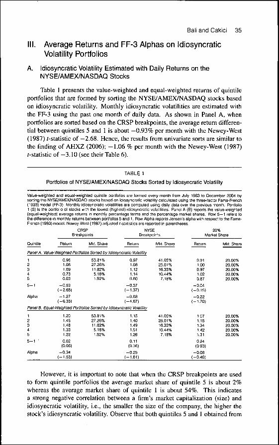
Table 1 presents the value-weighted and equal-weighted returns of quintileportfolios that are formed by sorting the NYSE/AMEX/NASDAQ stocks basedon idiosyncratic volatility. Monthly idiosyncratic volatilities are estimated withthe FF-3 using the past one month of daily data. As shown in Panel A, whenportfolios are sorted based on the CRSP breakpoints, the average return differen-tial between quintiles 5 and 1 is about —0.93% per month with the Newey-West(1987) ^-statistic of —2.68. Hence, the results from univariate sorts are similar tothe finding of AHXZ (2006); -1.06 % per month with the Newey-West (1987)f-statistic of -3.10 (see their Table 6).
TABLE 1
Portfolios of NYSE/AMEX/NASDAQ Stocks Sorted by Idiosyncratic Volatility
Value-weighted and equal-weighted quintile portfolios are formed every month from July 1963 to Deoember 2004 bysorting the NYSE/AMEX/NASDAQ stocks based on idiosyncratic volatility calculated using the three-factor Fama-French(1993) model (FF-3). fvlonthly idiosyncratic vclatiiities are computed using daiiy data over the previous month. Portfolio1 (5) is the portfoiio of stoci<s with the lowest (highest) idiosyncratic voiatilities. Panel A (B) reports the vaiue-weighted(equal-weighted) average returns in monthly percentage terms and the percentage market shares. Row 5 - 1 refers tothe difference in monthly returns between portfolios 5 and 1. Row Aipha reports Jensen's alpha with respect to the Fama-French (1993) model. Newey-West (1987) adjusted /-statistics are reported in parentheses.
Ouintile Return
CRSPBreakpoints
fvikt. Share
Br(
Return
NYSE3akpoints
Mkt. Share
Panel A. Value-Weighted Portfolios Sorted by Idiosyncratic Volatility
12345
5 - 1
Alpha
0.961.061.090.730.03
-0.93(-2.68)
-1.27(-6.33)
53.81%27.26%11.82%5.18%1.92%
0.971.081.121.140.60
-0.37(-1.37)
-0.68(-4.67)
41.05%25.01%16.33%10.44%7.18%
Panel B. Equal-Weighted Portfolios Sorted by Idiosyncratic Volatility
12345
5 - 1 •
Alpha
1.201.451.481.331.22
0.02(0.06)
-0.34(-1.53)
53.81%27.26%11.82%5.18%1.92%
1.151.401.491.511.26
0.11(0.36)
-0.25(-1.61)
41.05%25.01%16.33%10.44%7.18%
20%Market Share
Return
0.911.000.971.020.87
-0.04(-0.15)
-0 .22(-1.70)
1.071.151.341.421.31
0.24(0.93)
-0.06(-0.46)
Mkt. Share
20.00%20.00%20.00%20.00%20.00%
20.00%20.00%20.00%20.00%20.00%
However, it is important to note that when the CRSP breakpoints are usedto form quintile portfolios the average market share of quintile 5 is about 2%whereas the average market share of quintile 1 is about 54%. This indicatesa strong negative correlation between a firm's market capitalization (size) andidiosyncratic volatility, i.e., the smaller the size of the company, the higher thestock's idiosyncratic volatility. Observe that both quintiles 5 and 1 obtained from
36 Journal of Financial and Quantitative Analysis
the CRSP breakpoints contain 20% of the stocks sorted by idiosyncratic volatil-ity, but quintile 5 contains extremely small stocks generating substantially lowreturns (0.03% per month) as compared to quintile 1 that comprises large stocksproducing much higher returns (0.96% per month).
To generate quintile portfolios with a relatively more balanced average mar-ket share, we use the NYSE breakpoints, which is a more commonly used port-folio breakdown starting with Fama and French (1992). As shown in Panel A ofTable 1, the value-weighted average return difference between quintiies 5 and 1 isabout —0.37% with a f-statistic of — 1.37, indicating that the average return differ-ential is not statistically significant. That is, idiosyncratic risk cannot generate aneconomically or statistically significant average return difference when the NYSEbreakpoints are used to sort stocks into quintile portfolios.
Panel A of Table 1 shows that using the NYSE breakpoints does not entirelydiminish the extreme size differential of quintile portfolios because the NYSEsample also contains small stocks. In Panel A, the average market share of quin-tile 5 is about 7.2% whereas the average market share of quintile 1 is about 41%.To remove the concern about size differentials of quintile portfolios and to testwhether the idiosyncratic volatility effect is concentrated among small stocks,we generate quintile portfolios with an "equal" market share. With this portfo-lio formation, quintiies do not contain 20% of the stocks sorted by idiosyncraticvolatility, but they have an equal proportion of the market (i.e., 20%). Using thebreakpoint of "20% market share" diminishes the effect of firm size on the rela-tion between idiosyncratic risk and the cross section of expected returns. Panel Ashows that with the breakpoint of 20% market share, the value-weighted averagereturn differential between quintiies 5 and 1 is about —0.04% with a /-statistic of-0.15.
Panel B of Table 1 presents the equal-weighted average returns of quintileportfolios formed based on three different breakpoints (CRSP, NYSE, and 20%market share). The results provide no evidence for an economically or statisticallysignificant relation between idiosyncratic risk and the cross section of expectedreturns. When portfolios are sorted based on the CRSP breakpoints, the equal-weighted average return differential between quintiies 5 and 1 is about 0.02% permonth with a /-statistic of 0.06. The average return differentials obtained fromthe NYSE breakpoint and the equal market share of 20% are almost zero andstatistically insignificant.
In addition to the average raw returns, following AHXZ (2006), Table 1 alsopresents the magnitude and statistical significance ofthe intercepts (FF-3 alphas)from the regression of the value-weighted (or equal-weighted) portfolio returnson a constant, excess market return, SMB, and HML factors. As shown in PanelA of Table 1, the 5-1 differences in the FF-3 alphas for the CRSP and NYSEbreakpoints are negative and highly significant for the value-weighted portfolios.However, for the 20% market share, the 5—1 difference in FF-3 alphas is a smallnegative number with a /-statistic of — 1.70.
Panel B of Table 1 shows that for the equal-weighted portfolios the 5 -1 dif-ferences in the FF-3 alphas are small and statistically insignificant for all break-points considered in the paper (CRSP, NYSE, and 20% market share). Hence, the
Bali and Cakici 37
average raw returns and FF-3 alphas presented in Table 1 provide similar evidencefor the NYSE/AMEX/NASDAQ sample.
B. Idiosyncratic Volatility Estimated with Daily Returns on the NYSEStocks
The aforementioned results obtained for portfolios of stocks traded on theNYSE, AMEX, and NASDAQ indicate that there is no robustly significant re-lation between idiosyncratic volatility and the cross section of expected returns.There is a negative and significant relation between idiosyncratic risk and ex-pected returns only when the value-weighted portfolios are constructed based onCRSP breakpoints. This finding, which is also the main finding of AHXZ (2006),disappears when the equal-weighted average return differentials are comparedand/or when the portfolios are formed based on the NYSE breakpoint or the 20%market share.
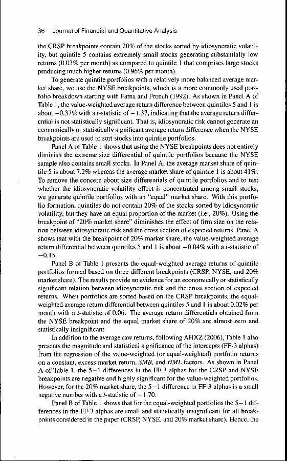
These results suggest that if there is a negative relation between idiosyncraticrisk and expected returns, it is just because of small stocks and the strong nega-tive relation between firms' market capitalization and idiosyncratic volatility. Toactually test this hypothesis, we consider relatively large stocks by excluding theNASDAQ and AMEX sample. We form quintile portfolios for the NYSE stocksusing the NYSE breakpoints. As presented in Table 2, both the value-weightedand equal-weighted average return differences between quintiles 5 and 1 are eco-nomically and statistically insignificant. A striking feature of Table 2 is that thevalue-weighted average return differential reduces from —0.93% to —0.23% permonth when portfolios are formed using the NYSE stocks with the NYSE break-points instead of using the NYSE/AMEX/NASDAQ stocks with the CRSP break-points.
Table 2 shows that even with the NYSE stocks there is a substantial differ-ence in the average market share of quintile portfolios. For example, the averagemarket share of quintile 5 is about 4% whereas the average market share of quin-tile 1 is about 44%. To remove the concern about size differentials of quintileportfolios, we generate quintile portfolios with an equal market share. As shownin Panel A of Table 2, the value-weighted average return difference between quin-tiles 5 and 1 (with 20% market share) is a small positive number, 0.09% permonth, and insignificant. Panel B of Table 2 indicates that with the 20% marketshare the equal-weighted average return differential between quintiles 5 and 1 ispositive, 0.41% per month, and statistically significant.
AHXZ (2006) are also concerned about the interaction of the idiosyncraticvolatility effect with firm size. To check the robustness of their findings, they,rank stocks based on idiosyncratic volatility using only NYSE stocks, and gen-erate quintile portfolios based on the NYSE stocks and the NYSE breakpoints.However, they do not report the average raw returns on idiosyncratic volatilityportfolios or the average return differential between quintiles 5 and 1. Instead,they present the magnitude and statistical significance of the intercepts (FF-3 al-phas) from the regression of the value-weighted portfolio returns on a constant,excess market return, SMB, and HML factors. As shown in AHXZ's Table 7, theintercepts (or the FF-3 alphas) are small and statistically insignificant for quin-
38 Journal of Financial and Quantitative Analysis
TABLE 2
Portfolios of NYSE Stocks Sorted by Idiosyncratic Volatility
Value-weighted and equal-weighted quintiie portfolios are formed every month from July 1963 to December 2004 bysorting the NYSE stocl<s based on idiosyncratic voiatility caicuiated using the three-factor Fama-French (1993) model (FF-3). Monthiy idiosyncratic voiatilities are computed using daiiy data over the previous month. Portfolio 1 (5) is the portfoiio ofstoci(s with the lowest (highest) idiosyncratic voiatilities. Panei A (B) reports the value-weighted (equai-weighted) averagereturns in monthiy percentage terms and the percentage market shares. Row 5—1 refers to the difference in monthlyreturns between portfolios 5 and 1. Row Aipha reports Jensen's alpha with respect to the Fama-French (1993) modei.Newey-West (1987) adjusted /-statistics are reported In parentheses.
NYSE Breakpoints 20% Market Share
Quintiie Return Mkt. Share Return
Panel A. Value-Weighted Portfolios of NYSE Stocks Sorted by idiosyncratic Voiatiiity
12345
5 - 1
Aipha
0.961.041.111.110.73
-0.23(-1.02)
-0.64(-4.40)
43.81%26.43%16.26%9.16%4.35%
0.910.990.980.991.00
0.09(0.49)
-0.18(-1.38)
Panei B. Equai-Weighted Portfoiios of NYSE Stoci<s Sorted by idiosyncratic Voiatiiity
12345
5 - 1
Alpha
1.161.401.541.611.40
0.24(1.03)
-0.31(-2.56)
43.81%26.43%16.26%9.16%4.35%
.08
.13
.33
.41
.49
0.41(2.16)
-0.01(-0.07)
fvikt. Share
20.00%20.00%20.00%20.00%20.00%
20.00%20.00%20.00%20.00%20.00%
tile portfolios 1, 2, 3, and 4. The FF-3 alpha is large and statistically significantonly for the highest idiosyncratic volatility portfolio. The highest quintile of id-iosyncratic volatility has an FF-3 alpha of —0.60% per month with a r-statistic of—5.14. Therefore, the 5—1 difference in FF-3 alphas is very large in magnitudeand statistically significant at —0.66% per month with a r-statistic of —4.85.
As indicated by AHXZ (2006), although restricting the whole universe ofstocks to NYSE diminishes the concern that the idiosyncratic volatility effect isconcentrated among small stocks, it does not completely remove this concern be-cause the NYSE sample still contains small stocks. Moreover, as discussed above,the economic and statistical significance of the 5 — 1 difference in FF-3 alphas isjust because of the highest idiosyncratic volatility portfolio, which contains verysmall stocks.
We also estimate the FF-3 alphas for the extended sample of July 1963-December 2004, and find similar results. While the FF-3 alphas are small andstatistically insignificant for quintile portfolios 1,2, 3, and 4, they are large andstatistically significant for the highest idiosyncratic volatility portfolio. Specifi-cally, as shown in Panel A of Table 2, the 5-1 difference in FF-3 alphas for thevalue-weighted portfolios is about —0.64% per month with a f-statistic of —4.40.
These results indicate that the difference in average raw returns betweenquintiles 5 and 1 is not similar to the 5—1 difference in FF-3 alphas. In fact, wedraw totally different conclusions from average raw returns and the FF-3 alphas.
Bali and Cakici 39
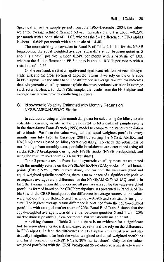
Specifically, for the sample period from July 1963-December 2004, the value-weighted average return difference hetween quintiies 5 and 1 is about -0.23%per month with a r-statistic of — 1.02, whereas the 5—1 difference in FF-3 alphasis about -0.64% per month with a ;-statistic of —4.40.
The more striking observation in Panel B of Table 2 is that for the NYSEbreakpoints, the equal-weighted average return differential between quintiies 5and 1 is a small positive number, 0.24% per month with a /-statistic of 1.03,whereas the 5 -1 difference in FF-3 alphas is about —0.31% per month with ar-statistic of -2.56.
On the one hand, we find a negative and significant relation between idiosyn-cratic risk and the cross section of expected returns if we rely on the differencein FF-3 alphas. On the other hand, the difference in average raw returns indicatesthat idiosyncratic volatility cannot explain the cross-sectional variation in averagestock returns. Hence, for the NYSE sample, the results from the FF-3 alphas andaverage raw returns provide conflicting evidence.
C. Idiosyncratic Volatility Estimated with Monthly Returns onNYSE/AMEX/NASDAQ Stocks
In addition to using within-month daily data for calculating the idiosyncraticvolatility measures, we utilize the previous 24 to 60 months of sample returnsin the three-factor Fama-French (1993) model to compute the standard deviationof residuals. We form the value-weighted and equal-weighted portfolios everymonth from July 1963 to December 2004 by sorting the NYSE, AMEX, andNASDAQ stocks based on idiosyncratic volatility. To check the robustness ofour findings from monthly data, portfolio breakdowns are determined using allstocks (CRSP breakpoints), using only NYSE stocks (NYSE breakpoints), andusing the equal market share (20% market share).
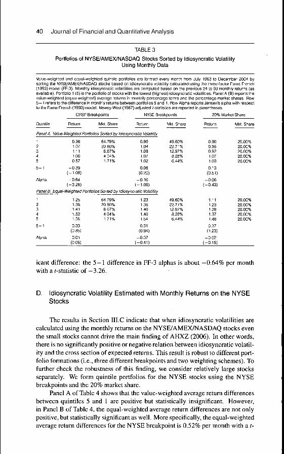
Table 3 presents results from the idiosyncratic volatility measures estimatedwith the monthly returns on the NYSE/AMEX/NASDAQ stocks. For all break-points (CRSP, NYSE, 20% market share) and for both the value-weighted andequal-weighted quintile portfolios, there is no evidence of a significantly positiveor negative average return difference for the NYSE/AMEX/NASDAQ stocks. Infact, the average return differences are all positive except for the value-weightedportfolios formed based on the CRSP breakpoints. As presented in Panel A of Ta-ble 3, with the CRSP breakpoints, the difference in average returns on the value-weighted quintile portfolios 5 and 1 is about —0.39% and statistically insignifi-cant. The highest average return difference is obtained from the equal-weightedportfolios with an equal market share of 20%. Panel B of Table 3 shows that theequal-weighted average return differential between quintiies 5 and 1 with 20%market share is positive, 0.37% per month, but statistically insignificant.
A striking feature of Table 3 is that there is no evidence for a significantlink between idiosyncratic risk and expected returns if we rely on the differencesin FF-3 alphas. In fact, the differences in FF-3 alphas are almost zero and sta-tistically insignificant for both the value-weighted and equal-weighted portfoliosand for all breakpoints (CRSP, NYSE, 20% market share). Only for the value-weighted portfolios with the CRSP breakpoint do we observe a negatively signif-
40 Journal of Financial and Quantitative Analysis
TABLE 3
Portfolios of NYSE/AMEX/NASDAQ Stocks Sorted by Idiosyncratic VolatilityUsing Monthly Data
Value.weighted and equal.weighted quintile portfolios are formed every month from July 1963 to December 2004 bysorting the NYSE/AMEX/NASDAO stocks based en idiosyncratic voiatiiity caicuiated using the three-faotor Fama-French(1993) modei (FF-3). Monthly idiosyncratic volatiiities are computed based on the previous 24 to 60 mcnthiy returns (asavaiiabie). Portfoiio 1 (5) is the portfolio of stocks with the iowest (highest) idiosynoratio volatilities. Panei A (B) reports thevalue-weighted (equal-weighted) average returns in monthiy percentage terms and the percentage market shares. Row5— 1 refers to the difference in monthly returns between portfolios 5 and 1. Row Aipha reports Jensen's aipha with respectto the Fama-French (1993) model. Newey-West (1987) adjusted (-statistics are reported in parentheses.
Quintiie
Panel A.
12345
5 - 1
Alpha
Panel B.
12345
5 - 1
Alpha
CRSP Breakpoints
Return filkt. Share
NYSE Breakpoints
Return
Value-Weighted Portfolios Sorted by Idiosyncratic Volatility
0.961.071.111.060.57
-0.39(-1.08)
-0.64(-3.26)
64.79%20.80%
8.67%4.04%1.71%
0.961.041.081.071.02
0.06(0.20)
-0 .16(-1.06)
Equal-Weighted Portfolios Sorted by Idiosyncratic Volatility
.25
.38
.41
.52
.58
0.33(0.85)
0.01(0.06)
64.79%20.80%8.67%4.04%1.71%
1.231.361.401.401.54
0.31(0.94)
-0.07(-0.41)
fvlkt. Share
49.60%22.71%12.97%8.28%6.44%
49.60%22.71%12.97%8.28%6.44%
20% Market Share
Return
0.900.950.921.071.03
0.13(0.51)
-0 .06(-0.43)
1.111.231.261.371.48
0.37(1.23)
-0.02(-0.15)
fvikt. Share
20.00%20.00%20.00%20.00%20.00%
20.00%20.00%20.00%20.00%20.00%
icant difference: the 5—1 difference in FF-3 alphas is about —0,64% per monthwith a/-statistic of—3,26,
D, Idiosyncratic Volatility Estimated with Monthly Returns on the NYSEStocks
The results in Section IILC indicate that when idiosyncratic volatilities arecalculated using the monthly returns on the NYSE/AMEX/NASDAQ stocks eventhe small stocks cannot drive the main finding of AHXZ (2006), In other words,there is no significantly positive or negative relation between idiosyncratic volatil-ity and the cross section of expected returns. This result is robust to different port-folio formations (i.e,, three different breakpoints and two weighting schemes). Tofurther check the robustness of this finding, we consider relatively large stocksseparately. We form quintile portfolios for the NYSE stocks using the NYSEbreakpoints and the 20% market share.
Panel A of Table 4 shows that the value-weighted average return differencesbetween quintiles 5 and 1 are positive but statistically insignificant. However,in Panel B of Table 4, the equal-weighted average return differences are not onlypositive, but statistically significant as well. More specifically, the equal-weightedaverage return differences for the NYSE breakpoint is 0,52% per month with a t-

Bali and Cakici 41
statistic of 1.94, and for the 20% market share it is about 0.48% per month with ar-statistic of 2.0.
TABLE 4
Portfolios of NYSE Stocks Sorted by Idiosyncratio Volatility Using Monthly Data
Value-weighted and equal-weighted quintile portfolios are formed every month from July 1963 to December 2004 bysorting the NYSE stocks based on idiosyncratic volatility calculated using the three-factor Fama-French (1993) model(FF-3). Monthly idiosyncratic volatilities are computed based on the previous 24 to 60 monthly returns (as available).Portfolio 1 (5) is tfie portfolio of stocks with the lowest (highest) idiosyncratic volatilities. Panel A (B) reports the value-weighted (equal-weighted) average returns in monthly percentage terms and the percentage market shares. Row 5 - 1refers to the difference in monthly returns between portfolios 5 and 1. Row Alpha reports Jensen's alpha with respect tothe Fama-French (1993) model. Newey-West (1987) adjusted (-statistics are reported in parentheses.
Quintile
Panel A.
12345
5 - 1
Alpha
Panel B.
12345
5 - 1
Alpha
NYSE Breakpoints
Return MM. Share Return
Value-Weighted Portfolios of NYSE Stocks Sorted by Idiosyncratic Volatility
0.951.031.051.041.15
0.20(0.79)
-0.11(-0.72)
53.67%23.82%11.98%6.94%3.59%
0.891.000.921.021.06
0.17(0.88)
-0.11(-0.87)
Equal-Weighted Portfolios of NYSE Stocks Sorted by Idiosyncratic Voiatility
1.161.321.431.441.68
0.52(1.94)
0.01(0.10)
53.67%23.82%11.98%6.94%3.59%
1.041.151.211.321.52
0.48(2.00)
0.04(0.26)
20% Market Share
Mkt. Share
20.00%20.00%20.00%20.00%20.00%
20.00%20.00%20.00%20.00%20.00%
For the equal-weighted portfolios, although we find a positive and significantlink between idiosyncratic risk and expected returns, there is no such evidence ifwe rely on the differences in FF-3 alphas, which are very small and statistically in-significant. Hence, for the equal-weighted portfolios of NYSE stocks, the resultsfrom FF-3 alphas and average raw returns provide confiicting evidence.
IV. Idiosyncratic Volatility Portfolios after a Screen for Size,Price, and Liquidity
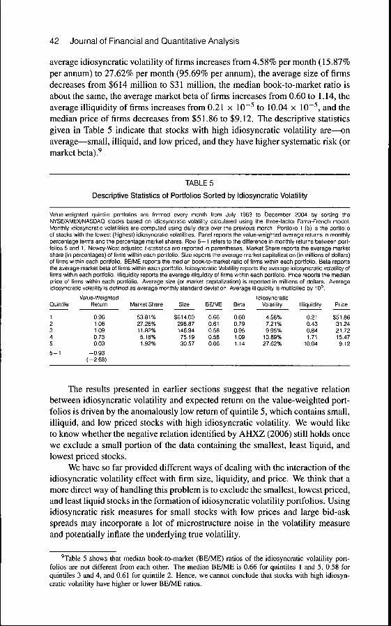
This section aims to clarify the source of a negative relation between id-iosyncratic volatility and expected returns on the value-weighted portfolios withCRSP breakpoints. Table 5 provides statistics for the value-weighted returns onthe quintile portfolios of NYSE/AMEX/NASDAQ stocks, average market share,average size, median book-to-market ratio, average market beta, average idiosyn-cratic volatility, average illiquidity, and median price of firms within each portfo-lio.^ When we move from a low volatility quintile to a high volatility quintile, the
"AS will be discussed below, stock illiquidity is measured by the ratio of absolute stock return toits dollar volume following Amihud (2002).
42 Journal of Financial and Quantitative Analysis
average idiosyncratic volatility of firms increases from 4.58% per month (15.87%per annum) to 21.62% per month (95.69% per annum), the average size of firmsdecreases from $614 million to $31 million, the median book-to-market ratio isabout the same, the average market beta of firms increases from 0.60 to 1.14, theaverage illiquidity of firms increases from 0.21 x 10~^ to 10.04 x 10^^, and themedian price of firms decreases from $51.86 to $9.12. The descriptive statisticsgiven in Table 5 indicate that stocks with high idiosyncratic volatility are—onaverage—small, illiquid, and low priced, and they have higher systematic risk (ormarket beta).^
TABLE 5
Descriptive Statistics of Portfolios Sorted by Idiosyncratic Volatility
Value-weighted quintile portfolios are formed every month from July 1963 to December 2004 by sorting theNYSE/AMEX/NASDAQ stooks based on idiosyncratic volatility calculated using the three-factor Fama-French model.Monthiy idiosyncratic volatilities are computed using daily data over the previous month. Portfoiio 1 (5) is the portfolioof stocks with the lowest (highest) idiosyncratic volatiiities. Panel reports the value-weighted average returns in monthiypercentage terms and the percentage market shares. Row 5—1 refers to the difference in monthly returns between port-folios 5 and 1. Newey-West adjusted (-statistics are reported in parentheses. Market Share reports the average marketshare (in percentages) of firms within each portfoiio. Size reports the average market capitalization (in miilions of dollars)of firms within each portfolio. BE/ME reports the median book-to-market ratio of firms within each portfolio. Beta reportsthe average market beta of firms within each portfolio. Idiosyncratic Volatility reports the average idiosyncratic volatility offirms within each portfolio. Illiquidity reports the average illiquidity of firms within each portfolio. Price reports the medianprice of firms within each portfolio. Average size (or market capitalization) is reported in miilions of dollars. Averageidiosyncratic volatility is defined as average monthly standard deviation. Average illiquidity is multiplied by 10^.
Quintile
123455 - 1
Value-WeightedReturn
0.961.061.090.730.03
-0.93(-2.68)
Market Share
53.81%27.26%11.82%5.18%1.92%
Size
$614.00298.87146.9475.1930.57
BE/ME
0.660.610.580.580.66
Beta
0.600.790.951.091.14
IdiosyncraticVolatiiity
4.58%7.21%9.95%
13.89%27.62%
Illiquidity
0.210.430.841.71
10.04
Price
$51.8631.2421.7215.479.12
The results presented in earlier sections suggest that the negative relationbetween idiosyncratic volatility and expected return on the value-weighted port-folios is driven by the anomalously low return of quintile 5, which contains small,illiquid, and low priced stocks with high idiosyncratic volatility. We would liketo know whether the negative relation identified by AHXZ (2006) still holds oncewe exclude a small portion of the data containing the smallest, least liquid, andlowest priced stocks.
We have so far provided different ways of dealing with the interaction of theidiosyncratic volatility effect with firm size, liquidity, and price. We think that amore direct way of handling this problem is to exclude the smallest, lowest priced,and least liquid stocks in the formation of idiosyncratic volatility portfolios. Usingidiosyncratic risk measures for small stocks with low prices and large bid-askspreads may incorporate a lot of microstructure noise in the volatility measureand potentially infiate the underlying true volatility.
'Table 5 shows that median book-to-market (BE/ME) ratios of the idiosyncratic volatility port-folios are not different from each other. The median BE/ME is 0.66 for quintiles 1 and 5, 0.58 forquintiles 3 and 4, and 0.61 for quintile 2. Hence, we cannot conclude that stocks with high idiosyn-cratic volatility have higher or lower BE/ME ratios.
Bali and Cakici 43
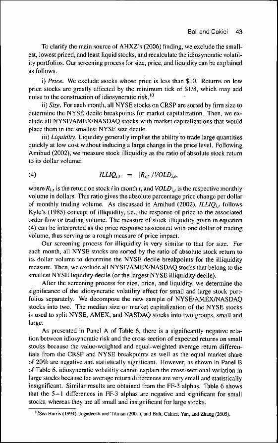
To clarify the main source of AHXZ's (2006) finding, we exclude the small-est, lowest priced, and least liquid stocks, and recalculate the idiosyncratic volatil-ity portfolios. Our screening process for size, price, and liquidity can be explainedas follows.
i) Price. We exclude stocks whose price is less than $10. Returns on lowprice stocks are greatly affected by the minimum tick of $1/8, which may addnoise to the construction of idiosyncratic risk.'°
ii) Size. For each month, all NYSE stocks on CRSP are sorted by firm size todetermine the NYSE decile breakpoints for market capitalization. Then, we ex-clude all NYSE/AMEX/NASDAQ stocks with market capitalizations that wouldplace them in the smallest NYSE size decile.
iii) Liquidity. Liquidity generally implies the ability to trade large quantitiesquickly at low cost without inducing a large change in the price level. FollowingAmihud (2002), we measure stock illiquidity as the ratio of absolute stock returnto its dollar volume:
(4) ILLlQi,, = \Ri^,\/VOLDi,,,
where /?,-,, is the return on stock i in month t, and VOLD,,, is the respective monthlyvolume in dollars. This ratio gives the absolute percentage price change per dollarof monthly trading volume. As discussed in Amihud (2002), ILLlQi, followsKyle's (1985) concept of illiquidity, i.e., the response of price to the associatedorder fiow or trading volume. The measure of stock illiquidity given in equation(4) can be interpreted as the price response associated with one dollar of tradingvolume, thus serving as a rough measure of price impact.
Our screening process for illiquidity is very similar to that for size. Foreach month, all NYSE stocks are sorted by the ratio of absolute stock return toits dollar volume to determine the NYSE decile breakpoints for the illiquiditymeasure. Then, we exclude all NYSE/AMEX/NASDAQ stocks that belong to thesmallest NYSE liquidity decile (or the largest NYSE illiquidity decile).
After the screening process for size, price, and liquidity, we determine thesignificance of the idiosyncratic volatility effect for small and large stock port-folios separately. We decompose the new sample of NYSE/AMEX/NASDAQstocks into two. The median size or market capitalization of the NYSE stocksis used to split NYSE, AMEX, and NASDAQ stocks into two groups, small andlarge.
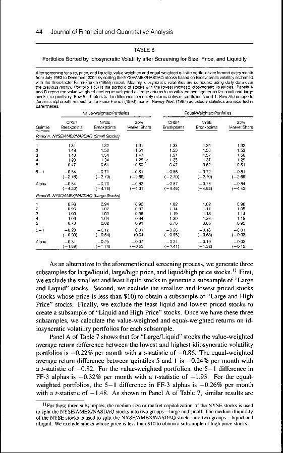
As presented in Panel A of Table 6, there is a significantly negative rela-tion between idiosyncratic risk and the cross section of expected returns on smallstocks because the value-weighted and equal-weighted average return differen-tials from the CRSP and NYSE breakpoints as well as the equal market shareof 20% are negative and statistically significant. However, as shown in Panel Bof Table 6, idiosyncratic volatility cannot explain the cross-sectional variation inlarge stocks because the average return differences are very small and statisticallyinsignificant. Similar results are obtained from the FF-3 alphas. Table 6 showsthat the 5—1 differences in FF-3 alphas are negative and significant for smallstocks, whereas they are all small and insignificant for large stocks.
'"See Harris (1994), Jegadeesh and Titman (2001), and Bali, Cakici, Yan, and Zhang (2005).
44 Journal of Financial and Quantitative Analysis
TABLE 6
Portfolios Sorted by Idiosyncratic Volatility after Screening for Size, Price, and Liquidity
After screening for size, price, and liquidity, value-weighted and equai-weighted quintile portfolios are formed every montfifrom July 1963 to December 2004 by sorting the NYSE/AMEX/NASDAQ stocks based on idiosyncratic volatility estimatedwith the three-factor Fama-French (1993) modei. Monthiy idiosyncratic vclatiiities are computed using daily data overthe previous month. Portfolio 1 (5) is the portfolio of stocks with the lowest (highest) idiosyncratic volatilities. Panels Aand B report the value-weighted and equal-weighted average returns in monthly percentage terms for small and largestocks, respectively. Row 5—1 refers to the difference in monthly returns between portfolios 5 and 1. Row Alpha reportsJensen's alpha with respect to the Fama-French (1993) model. Newey-West (1987) adjusted (-statistics are reported inparentheses.
Value-Weighted Portfolios Equal-Weighted Portfolios
Quintiie
Panel A.
12345
5 - 1
Alpha
Panel B.
12345
5 - 1
Alpha
CRSPBreakpoints
NYSEBreakpoints
NYSE/AMEX/NASDAQ (Small Stocks)
1,311.481.481.200.47
-0.84(-2.76)
-0.84(-4.30)
1.321.521.541.340.61
-0.71(-2.70)
-0.76(-4.78)
NYSE/AMEX/NASDAQ (Large Stocks)
0.960.961.001.060.73
-0.23(-0.93)
-0.31(-1.89)
0.941.021.031.040.82
-0.12(-0.54)
-0,25(-1,74)
20%Market Share
1.311.511.471.25 /0.50
-0.81(-2,69)
-0.82(-4,31)
0.900.970.960,940,91
0,01(0,04)
-0,07(-0,53)
CRSPBreakpoints
1.331.501.511.250.47
-0.86(-2,79)
-0,87(-4.46)
1,021,141,191,200,76
-0,26(-0,95)
-0,24(-1.41)
NYSEBreakpoints
1.341.531.571.370.62
-0,72(-2.70)
-0 ,78(-4,85)
1,021,171,181,230,86
-0,16(-0,68)
-0,19(-1,32)
20%Market Share
1,321,531,501,290,51
-0,81(-2,69)
-0,84(-4,43)
0,961,051,141,150,95
-0,01(-0,03)
-0 ,02(-0,15)
As an alternative to the aforementioned screening process, we generate threesubsamples for large/liquid, large/high price, and liquid/high price stocks." First,we exclude the smallest and least liquid stocks to generate a subsample of "Largeand Liquid" stocks. Second, we exclude the smallest and lowest priced stocks(stocks whose price is less than $10) to obtain a subsample of "Large and HighPrice" stocks. Finally, we exclude the least liquid and lowest priced stocks tocreate a subsample of "Liquid and High Price" stocks. Once we have these threesubsamples, we calculate the value-weighted and equal-weighted returns on id-iosyncratic volatility portfolios for each subsample.
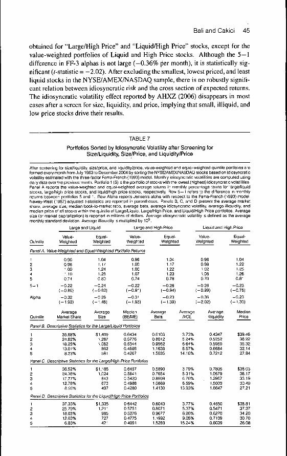
Panel A of Table 7 shows that for "Large/Liquid" stocks the value-weightedaverage return difference between the lowest and highest idiosyncratic volatilityportfolios is —0.22% per month with a ^-statistic of —0.86. The equal-weightedaverage return difference between quintiies 5 and 1 is —0.24% per month witha i-statistic of —0.82. For the value-weighted portfolios, the 5—1 difference inFF-3 alphas is —0.32% per month with a r-statistic of —1.93. For the equal-weighted portfolios, the 5 — 1 difference in FF-3 alphas is —0.26% per monthwith a f-statistic of —1.48. As shown in Panel A of Table 7, similar results are
' ' For these three subsamples, the median size or market capitalization of the NYSE stocks is usedto split the NYSE/AMEX/NASDAQ stocks into two groups—large and small. The median illiquidityof the NYSE stocks is used to split the NYSE/AMEX/NASDAQ stocks into two groups—liquid andilliquid. We exclude stocks whose price is less than $tO to obtain a subsample of high price stocks.
Bali and Cakici 45
obtained for "Large/High Price" and "Liquid/High Price" stocks, except for thevalue-weighted portfolios of Liquid and High Price stocks. Although the 5—1difference in FF-3 alphas is not large (—0.36% per month), it is statistically sig-nificant (/-statistic - —2.02). After excluding the smallest, lowest priced, and leastliquid stocks in the NYSE/AMEX/NASDAQ sample, there is no robustly signifi-cant relation between idiosyncratic risk and the cross section of expected returns.The idiosyncratic volatility effect reported by AHXZ (2006) disappears in mostcases after a screen for size, liquidity, and price, implying that small, illiquid, andlow price stocks drive their results.
TABLE 7
Portfolios Sorted by Idiosyncratic Voiatiiity after Screening forSize/Liquidity, Size/Price, and Liquidity/Price
After screening for size/liquidity, size/price, and liquidity/price, vatue.weigfited and equal-weighted quintile portfolios areformed every month from July 1963 to December 2004 by sorting the NYSE/AMEX/NASDAQ sloci<s based on idiosyncraticvolaliiily estimated with Ihe three-factor Fama-French (1993) model. Monthly idiosyncratic voiatilities are computed usingdaiiy data over the previous month. Portfoiio 1 (5) is the portfolio of stocl<s with the lowest (highest) idiosyncratic volatiiities.Panel A reports the value-weighted and equal-weighted average returns in monthly percentage terms for large/liquidstocks, large/high price stoci<s, and liquid/high price stocks, respectively. Row 5—1 refers to the difference in monthlyreturns between portfolios 5 and 1. Row Alpha reports Jensen's alpha with respect to the Fama-French (1993) model.Newey-West (1987) adjusted (-statistics are reported in parentheses. Paneis B, C, and D present the average marketshare, average size.-median book-to-market ratio, average beta, average idiosyncratic volatility, average iiiiquidity, andmedian price of all stocks within the quintile of Large/Liquid, Large/High Price, and Liquid/High Price portfolios. Averagesize (or market capitalization) is reported in miliions of doilars. Average idiosyncratic voiatiiity is defined as the averagemonthly standard deviation. Average iiiiquidity is muitiplied by 10^.
Large and Liquid Large and High Price Liquid and i-ligh Price
Ouintile
Panel A.
1
345
6 - 1
Alpha
Quintile
Panel B.
12345
Panel C.
1eg
345
Value-Weighted
Equal-Weighted
Value-Weighted
Value-Weighted and Equal-Weighted Portfolio Returns
0.960.981.001.100.74
-0.22(-0.86)
-0.32(-1.93)
AverageMarket Share
1.041.171.241.280.80
-0.24(-0.82)
-0 .26(-1.48)
AverageSize
0.961.001.001.070.74
-0.22(-0.91)
-0.31(-1.93)
Median(BE/ME)
Descriptive Statistics for the Large/Liquid Portfolios
35.68%24.82%18.25%13.01%8.23%
$1,4091,2871,082
862581
0.64340.57760.53440.48880.4267
Descriptive Statistics for the Large/High Price Portfolioi
36.52%24.38%17.77%12.78%8.55%
$1,1881,024
843673497
0.64570.58410.54200.49880.4280
Equal-Weighted
1.041.171.221.230.78
-0.26(-0.94)
-0.23(-1.39)
AverageBeta
0.61030.80120.95621.16381.5035
0.58900.76540.89981.08691.4130
Panel D. Descriptive Statistics for the Liquid/High Price Portfolios
12345
37.33%25.79%18.03%12.03%6.83%
$1,3351,211
985727421
0.64420.57510.52760.47750.4091
0.60430.80710.96771.19921.5289
AverageIVOL
3.73%5.24%6.64%8.57%
14.16%
3.79%5.31%6.70%8.59%
13.93%
3.77%5.37%6.90%9.05%
15.24%
Value-Weighted
0.960.981.021.060.70
-0.26(-0.99)
-0 .36(-2.02)
AverageIiiiquidity
0.43470.52520.59590.66840.7212
0.78051.05791.29671.50031.6647
0.45500.54710.62700.71090.8009
Equal-Weighted
1.041.221.251.260.81
-0.23(-0.78)
-0.23(-1.30)
MedianPrice
$39.4638.2235.3232.1427.84
$38.0336.1733.1930.4927.21
$38.8137.3734.2030.7026.08
46 Journal of Financial and Quantitative Analysis
Table 7 also provides descriptive statistics for the idiosyncratic volatilityportfolios of large, liquid, and high price stocks. Panels B, C, and D present theaverage market share, average size, median book-to-market ratio, average beta,average idiosyncratic volatility, average illiquidity, and median price of all stockswithin each quintile of Large/Liquid, Large/High Price, and Liquid/High Priceportfolios. The qualitative results are very similar for all three subsamples: Af-ter eliminating the smallest, least liquid, and lowest priced stocks, the descriptivestatistics indicate that stocks with high idiosyncratic volatility are—on average—small, illiquid, low priced, and have high market beta and low book-to-marketratios.
V. Results from Inverse Volatility-Weighted Portfolios
We have so far shown that the negative relation between idiosyncratic riskand expected return is concentrated among small, illiquid, and low price stockswith high idiosyncratic volatility. To deal with the interaction of the idiosyncraticvolatility effect with firm size, AHXZ (2006) use the value-weighted portfolios.However, using the value-weighted portfolios does not lessen the effect of firmsize on the relation between idiosyncratic volatility and expected returns.
First, as shown in Table 1, when portfolios are formed based on the CRSPbreakpoints the value-weighted average return of quintile 5 is extremely low(0.03% per month), especially compared to the value-weighted average returnof quintile 1 (0.96% per month). Second, the value-weighted average return ofquintile 5 (0.03% per month) is much lower than the equal-weighted average re-turn of quintile 5 (1.22% per month). To understand these differences, we focuson quintile 5 which contains stocks with the highest idiosyncratic volatility andthe smallest market capitalization.
It is important to clarify why there is a considerable difference between thevalue-weighted and the equal-weighted average return ofthe same portfolio (quin-tile 5). Although quintile 5 from the CRSP breakpoints contains 20% ofthe stockssorted by idiosyncratic volatility, it represents only a small proportion ofthe valueof the market (less than 2% on average). It is well known that small stocks havehigher average returns than large stocks, which suggests that quintile 5 shouldactually contain stocks with higher returns. In fact, this is exactly what we findwhen we compute the equal-weighted average return of quintile 5, 1.22% permonth. However, since the market capitalizations of very small stocks in quintile5 are drastically low, the value-weighted average return of quintile 5 turns out tobe much lower than the equal-weighted average return of the same quintile.
This is due to the utilization of very small stocks in the construction of thevalue-weighted portfolios. Note that small stocks are treated differently when de-termining the breakpoints and when computing the average returns of the volatil-ity portfolios. Specifically, when sorting stocks into quintile portfolios basedon their idiosyncratic volatility we do consider small stocks in determining thebreakpoints. However, once the breakpoints are determined and the portfoliosare constructed, small stocks are practically excluded when calculating the value-weighted return of quintile 5. Since the market capitalizations of small stocks inquintile 5 are very small, extremely low weights (practically zero weights) are
Bali and Cakici 47
given to very small stocks with high returns. Although the returns of very smallstocks in quintile 5 are high, the value-weighted average return of the portfolio(quintile 5) is low just because of extremely low market capitalization weights.'^
Although the value weighting scheme gives lower weight to small stocks, itdoes not eliminate the interaction of the idiosyncratic volatility effect with firmsize (especially in quintile 5). In fact, the Appendix clarifies that the only reasonfor the existence of a negative relation between idiosyncratic risk and expectedreturns is the value weighting scheme used in the highest idiosyncratic volatilityquintile (i.e., quintile 5). We further examine this issue by using the inverse id-iosyncratic volatility-weighted portfolios. Specifically, we weight stocks in quin-tile portfolios by the inverse of their idiosyncratic volatility rather than by theirmarket capitalization.'-' This method gives lower weight to those stocks withhigher idiosyncratic volatility.
This alternative weighting scheme sheds light on the true underlying relationbetween idiosyncratic volatility and expected returns. As shown in Table 1, theequal-weighted average return of quintile 5 is 1.22% per month and note that theequal-weighted portfolios do not give lower (higher) weight to those stocks withhigher (lower) idiosyncratic volatility. If the true relation between idiosyncraticrisk and expected return is negative, then we expect the inverse volatility-weightedaverage return of quintile 5 to be higher than 1.22% per month since low volatilitystocks are expected to have higher returns and this method gives more weight tothose stocks with lower volatility. Similarly, if the true relation is negative, thenhigh volatility stocks are expected to have lower returns and this method giveslower weight to those stocks with higher volatility.
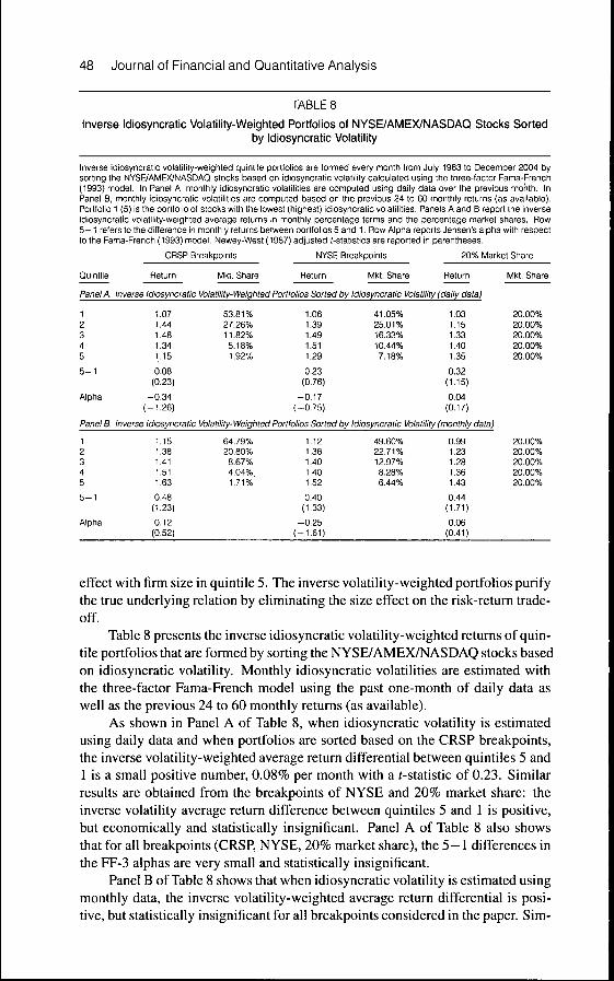
However, Table 8 shows that when idiosyncratic volatility is estimated usingdaily data and when the NYSE/AMEX/NASDAQ stocks are sorted based on theCRSP breakpoints, the inverse volatility-weighted average return of quintile 5 is1.15% per month, which is less than 1.22% per month. This finding providesfurther evidence against the existence of a negative risk-return trade-off.
If the true relation between idiosyncratic risk and expected return is positive,then we expect the inverse volatility-weighted average return of quintile 5 to belower than 1.22% per month since low volatility stocks are expected to have lowerreturns, and this method gives higher weight to those stocks with lower volatility.Similarly, if the true relation is positive, then high volatility stocks are expectedto have higher returns and this method gives lower weight to those stocks withhigher volatility. Although 1.15% is lower than 1.22%, the difference (0.07% permonth) is not significant enough to claim that the true relation is strongly positive.Overall, these results indicate that if there is a link between idiosyncratic volatilityand expected returns, it is not negative. It is positive, but insignificant.
The Appendix shows that the negative relation between idiosyncratic riskand expected returns is caused by the interaction of the idiosyncratic volatility
'-The Appendix clarifies the source of average return differences between the value- and equal-weighted portfolios.
'•'Cohen and Polk (1998) use the inverse idiosyncratic volatility-weighted portfolios of book-to-market (BE/ME) ratios to show that average returns to industry-based BE/ME portfolios are positive,statistically significant, and persistent. They find that the performance of inverse volatility-weightedBE/ME portfolios is significantly improved in risk-adjusted terms when implemented in its industry-neutral hedging form.
48 Journal of Financial and Quantitative Analysis
TABLE 8
Inverse Idiosyncratic Volatility-Weighted Portfolios of NYSE/AMEX/NASDAQ Stocks Sortedby Idiosyncratic Volatility
Inverse idiosyncratic volaliiity-weighted quintile portfolios are formed every month from Juiy 1963 to December 2004 bysorting the NYSE/AMEX/NASDAQ stocks based on idiosyncratic voiatiiity caicuiated using the three-factor Fama-French(1993) modei. in Panel A, monthiy idiosyncratic volatiiities are computed using daiiy data over the previous month. InPanel B, montiiiy idiosyncratic voiatilities are computed based on the previous 24 to 60 monthiy returns (as available).Portfoiio 1 (5) is the portfoiio of stocks with the lowest (highest) idiosyncratic voiatilities. Panels A and B report the inverseidiosyncratic voiatiiity-weighted average returns in monthiy percentage terms and the percentage market shares. Row5—1 refers to the difference in monthiy returns between portfoiios 5 and 1. Row Aipha reports Jensen's aipha with respectto the Fama-French (1993) modei. Newey-West (1987) adjusted Nstatistics are reported in parentheses.
Quintiie
Panei A.
12345
5 - 1
Alpha
Panei B.
12345
5 - 1
Alpha
CRSP Breakpoints
Return Mkt. Share
NYSE Breakpoints
Return Mkt. Share
20% Market Share
Return
inverse idiosyncratic Voiatiiity-Weighted Portfoiios Sorted by idiosyncratic Voiatiiity (daily data)
1.071.441.481.341.15
0.08(0.23)
-0.34(-1.26)
53.81%27.26%11.82%5.18%1.92%
1.061.391.491.511.29
0.23(0.76)
-0.17(-0.75)
41.05%25.01%16.33%10.44%7.18%
1.031.151.331.401.35
0.32(1.15)
0.04(0.17)
Inverse Idiosyncratic Voiatiiity-Weighted Portfciios Sorted by idiosyncratic Voiatiiity (monthiy data)
1.151.381.411.511.63
0.48(1.23)
0.12(0.52)
64.79%20.80%
8.67%4.04%,1.71%
1.121.361.401.401.52
0.40(1.33)
-0.25(-1.61)
49.60%22.71%12.97%8.28%6.44%
0.991.231.281.361.43
0.44(1.71)
0.06(0.41)
Mkt. Share
20.00%20.00%20.00%20.00%20.00%
20.00%20.00%20.00%20.00%20.00%
effect with firm size in quintile 5. The inverse volatility-weighted portfolios purifythe true underlying relation by eliminating the size effect on the risk-return trade-off.
Table 8 presents the inverse idiosyncratic volatility-weighted returns of quin-tile portfolios that are formed by sorting the NYSE/AMEX/NASDAQ stocks basedon idiosyncratic volatility. Monthly idiosyncratic volatilities are estimated withthe three-factor Fama-French model using the past one-month of daily data aswell as the previous 24 to 60 monthly returns (as available).
As shown in Panel A of Table 8, when idiosyncratic volatility is estimatedusing daily data and when portfolios are sorted based on the CRSP breakpoints,the inverse volatility-weighted average return differential between quintiles 5 and1 is a small positive number, 0.08% per month with a /-statistic of 0.23. Similarresults are obtained from the breakpoints of NYSE and 20% market share: theinverse volatility average return difference between quintiles 5 and 1 is positive,but economically and statistically insignificant. Panel A of Table 8 also showsthat for all breakpoints (CRSP, NYSE, 20% market share), the 5 -1 differences inthe FF-3 alphas are very small and statistically insignificant.
Panel B of Table 8 shows that when idiosyncratic volatility is estimated usingmonthly data, the inverse volatility-weighted average return differential is posi-tive, but statistically insignificant for all breakpoints considered in the paper. Sim-
Bali and Cakici 49
ilar results are obtained from the differences in FF-3 alphas. For all breakpoints,the 5-1 differences in FF-3 alphas are economically and statistically insignifi-cant. Overall, the average raw returns and the FF-3 alphas presented in Table 8provide similar evidence and indicate that the idiosyncratic volatility effect re-ported by AHXZ (2006) dies out after giving relatively lower (higher) weights tothose stocks with higher (lower) idiosyncratic volatility.
VI. Relative Accuracy of the Monthly Idiosyncratic VolatilityMeasures
As discussed in earlier sections, our cross-sectional tests use two differentmeasures of monthly idiosyncratic volatility. One measure (denoted by lVOL'''"'^)is the monthly realized idiosyncratic volatility obtained from daily returns overthe previous month and the other measure (denoted by IVOL'""'"'''^') is also themonthly realized idiosyncratic volatility, but it is based on the previous 24 to60 monthly returns (as available). Both measures are "unconditional" standarddeviations of residuals from the OLS estimation of the FF-3:
= a,-,, + (3i,,{Rm,t - r/,,) +
where the unconditional realized idiosyncratic volatility is defined as E{ef,\f2,-\)
The critical difference between these two monthly realized idiosyncraticvolatility measures is that there is a negative and significant relation betweenlYQldaiiy j , ^ ^ ji g , Q5g section of expected returns (as indicated by AHXZ (2006)),whereas the cross-sectional relation between IVOL"'"'"'''^ and expected stock re-turns is flat. As discussed in detail, the strong negative relation obtained fromIVOU''"'^ is due to the value weighting scheme that yields an anomalously lowreturn of quintile 5, which contains very small, illiquid, and low priced stocks.When different weighting schemes, and large, liquid, and high priced stocks areconsidered, the negative relation with IVOU'"''^ disappears. This suggests thatthe IVOL'^'"'^ measure obtained from daily data can be subject to all sorts of mar-ket microstructure problems, such as asynchronous trading and bid-ask bounce,which can potentially disturb the time-series pattern of the underlying true volatil-ity.
Table 9 reports descriptive statistics for the time series of monthly idiosyn-cratic volatility measures {IVOL''""^ and IVOL'""""''^'). First, we compute the mean,median, maximum, minimum, standard deviation, skewness, and kurtosis statis-tics for the time series of IVOL''''"y and IVOL"'°""''^ for each stock trading on theNYSE, AMEX, and NASDAQ.'" Then, we present the 1 to 99 percentiles of thesedescriptive statistics. As shown in Panel A of Table 9, the daily measure of id-iosyncratic volatility is clearly too noisy and exhibits significant departures fromnormality. Specifically, the standard deviation of IVOL'''"'^ is very large comparedto its mean, and the empirical distribution of IVOL''"''^ is a highly skewed and lep-tokurtic. The skewness statistics of lVOU'""^ are in the range of 0.80 to 11.74 and
'^The median correlation between lVOL'''"'y and /voi,'""""''-' is about 14.77% for the overallsample.

50 Journal of Financial and Quantitative Analysis
the kurtosis statistics of IVOU'''"y are in the range of 2,76 to 165,88. These highlysignificant skewness and excess kurtosis statistics provide evidence that IVOL''"''^is a highly noisy measure of expected future volatility. The maximum and min-imum values of IVOU'"'^^ strongly support this conclusion. Panel B of Table 9shows that the monthly measure of idiosyncratic volatility is much more stableand its empirical distribution is much closer to normal. As compared to IVOL^"''^,the skewness, kurtosis, maximum, and minimum values of IVOL'"""''''^ are verysmall, and only 10% of the overall sample of IVOL"^""''^ shows departures fromnormality.
TABLE 9
Descriptive Statistics for the Monthly Idiosyncratic Volatility Measures
Table 9 reports the 1 to 99 percentiles of mean, median, maximum, minimum, standard deviation, skewness, and kurtosisstatistics of monthiy reaiized idiosyncratic voiatiiity measures. Monthiy realized idiosyncratic voiatiiity is computed eitherusing daily data over the previous month (/VO/.'*^'^) or using the previous 24 to 60 monthly returns (/i/o/.'"°"'™>'). Panei A(Panel B) reports descriptive statistics for the time series of tVOL''^''^ ^ivoL""""^^).
Percentile
1 5 10 20 30 40
Panel A. Descriptive Statistics for the Time Series of IVOL'^^'^
MeanMedianMaximumMinimumStd. dev.SkewnessKurtosis
0.00220.00100.01230.00000.00220.79562.7588
0.00370.00210.02450.00000.00391.25254.0690
0.00510.00300.03500.00000.00551.54275.1639
0.00790.00480.05670.00000.00881.94517.1003
0.01130.00680.08320.00020.01272.29169.1158
0.01570.00950.11910.00040.01832.626011.373
Panel B. Descriptive Statistics for the Time Series of IVOL"'"""^'^
MeanMedianMaximumMinimumStd. dev.SkewnessKurtosis
0.00190.00170.00310.00080.0003
-0.69151.1774
0.00320.00300.00520.00140.0007-0.55311.4074
0.00430.00400.00710.00200.0010
-0.44271.5575
0.00650.00600.01100.00310.0016-0.29981.7660
0.00930.00860.01570.00450.0023-0.06981.9558
0.01270.01170.02110.00610.00330.12322.1394
50
0.02170.01300.16850.00070.02582.994714.165
0.01680.01540.02800.00820.00440.29892.3497
60
0.02990.01750.23990.00120.03703.437417.872
0.02210.02030.03700.01090.00610.48752.6150
70
0.04230.02380.35290.00190.05423.999423.241
0.02930.02710.04950.01480.00860.71022.9829
80
0.0614
90
0.10150.0339 0.05300.55340.00320.08464.811431.832
0.04090.03820.06810.02080.01271.01233.6802
1.02000.00610.15436.360952.867
0.06380.06020.10620.03340.02211.52865.2597
95
0.14890.07671.63310.00980.23847.970380.181
0.09180.08740.16120.04780.03592.09327.6835
99
0.28450.14523.41120.02330.509811.744165.88
0.19120.18790.36450.10240.09933.726419.105
To determine whether I'VOL''"''^ or IVOL'"""''''^ provides more accurate pre-dictions of expected future volatility of monthly returns, we use two benchmarksof conditional idiosyncratic volatility:
(5) f^i,t-rf^, = ai,,-i-l3i,,{R^^, - rf^,)-¥
(6)
(7)
GARCH:
= af, = exp
where equation (6) is the GARCH{1,1) model of Bollerslev (1986) that definesthe current conditional variance of monthly returns as a function of the last pe-
Bali and Cakici 51
Hod's unexpected news (or squared information shocks, e^,_]) and the last pe-riod's conditional variance (cr?,_|). We use the GARCH{1,1) model of Boller-slev (1986) because of its simplicity and its easy to follow properties for timeaggregation and stationarity. However, it has well-known drawbacks.
In a symmetric GARCH process shown in equation (6), positive and nega-tive return shocks of the same magnitude produce the same amount of volatility.Hence, the GARCH model of BoUerslev (1986) cannot cope with the skewnessof log price changes. That is, one can expect that forecasts and forecast errorvariances from a symmetric GARCH model may be biased for skewed return se-ries. Also, larger return shocks forecast more volatility at a rate proportionalto the square of the size of the return shock. If a positive shock causes morevolatility than a negative shock of the same size, the symmetric GARCH modelunderpredicts the amount of volatility following positive shocks and overpredictsthe amount of volatility following negative shocks. Furthermore, if large returnshocks cause more volatility than a quadratic function allows, then the symmetricGARCH model underpredicts volatility after a large return shock and overpredictsvolatility after a small return shock.
Several modifications of the GARCH model that explicitly take account ofskewed distributions have been proposed. In this paper, we consider one suchmodification, in which good news and bad news have different predictability forfuture volatility. Equation (7) is the exponential GARCH, EGARCH{\, 1), modelof Nelson (1991), which parameterizes the conditional variance as a nonlinearasymmetric function of unexpected information shocks to the stock market. Pa-rameter 6\ allows for an asymmetric volatility response to past positive and nega-tive return shocks. In general, 6\ is estimated to be significantly negative for stockreturns, and with ^i < 0 negative price changes are followed by greater increasesin variance than equally large positive price changes.
We measure expected future volatility with the conditional standard devia-tion of monthly stock returns. Specifically, the square root of the conditional vari-ance estimates from the GARCH{\, 1) and EGARCH{1,1) models are used as avolatility benchmark: af^'^'^^ and af^'^'^CH ^^ computed as Juf, from equations(6) and (7), respectively.
When testing the relative accuracy of IVOL''''"y and IVOL""""'''y, we use boththe in-sample and out-of-sample estimates of conditional idiosyncratic volatil-ity. First, we generate the in-sample conditional idiosyncratic volatility measures^^CARCH^ ^EGARCH^ based on the maximum likelihood parameter estimates of allstocks trading on the NYSE, AMEX, and NASDAQ.'^ Second, for each monthfrom July 1963 to December 2004, we generate the out-of-sample conditional id-iosyncratic volatility measures {a^f^^", af^^'^^") for all NYSE/AMEX/NASDAQstocks using the previous 60 monthly returns in our sample. Specifically, the pre-vious month's GARCH {or EG ARCH) estimate ofthe conditional standard devia-tion is used as the estimate for this month's conditional idiosyncratic risk measure.Finally, to compare the relative accuracy oflVOU'''''^ and IVOL"'""''''^, we run thefollowing OLS regressions for each firm i and for each time t:
require firms to have more than 30 monthly returns to be eligible for in-sample maximumlikelihood estimation.
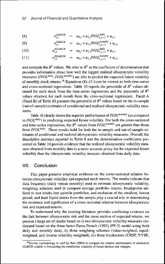
52 Journal of Financial and Quantitative Analysis
(8)
(9)
(10)
(11)
GARCHi,t
^GARCHi,l
^EGARCH
^EGARCH
and compute the R^ values. We refer to R^ as the coefficient of determination thatprovides information about how well the lagged realized idiosyncratic volatilitymeasures iIVOL''''''y, {VOL""""'''y) are able to predict the expected future volatilityof monthly stock returns.'^ Equations (8)-(l 1) can be viewed as both time-seriesand cross-sectional regressions. Table 10 reports the percentiie of R^ values ob-tained for each stock from the time-series regressions and the percentiie of /?^values obtained for each month from the cross-sectional regressions. Panel A(Panel B) of Table 10 presents the percentiie of R^ values based on the in-sample(out-of-sample) estimates of conditional and realized idiosyncratic volatility mea-sures.
Table 10 clearly shows the superior performance of IVOL""'"''''^ (as comparedto IVOL''^''y) in predicting expected future volatility. For both the cross-sectionaland time-series regressions, the R^ values from IVOL""'"''''^ are greater than thosefrom IVOL'''"'y. These results hold for both the in-sample and out-of-sample es-timates of conditional and realized idiosyncratic volatility measures. Overall, thedescriptive statistics reported in Table 9 and the determination coefficients pre-sented in Table 10 provide evidence that the realized idiosyncratic volatility mea-sure obtained from monthly data is a more accurate proxy for the expected futurevolatility than the idiosyncratic volatility measure obtained from daily data.
VII. Conclusion
This paper presents empirical evidence on the cross-sectional relation be-tween idiosyncratic volatility and expected stock returns. The results indicate thatdata frequency (daily versus monthly) used to estimate idiosyncratic volatility,weighting schemes used to compute average portfolio returns, breakpoints uti-lized to sort stocks into quintile portfolios, and exclusion of the smallest, lowestpriced, and least liquid stocks from the sample play a crucial role in determiningthe existence and significance of a cross-sectional relation between idiosyncraticrisk and expected returns.
To understand why the existing literature provides confiicting evidence onthe link between idiosyncratic risk and the cross section of expected returns, wepresent a large set of results based on i) two idiosyncratic volatility measures (es-timated based on the three-factor Fama-French (1993) (FF-3) model using bothdaily and monthly data), ii) three weighting schemes (value-weighted, equal-weighted, and inverse volatility-weighted), iii) three breakpoints (CRSP, NYSE,
'^Similar methodology is used by Bali (2000) to compare the relative performance of alternativeGARCH models in forecasting the conditional volatility of future interest rate changes.
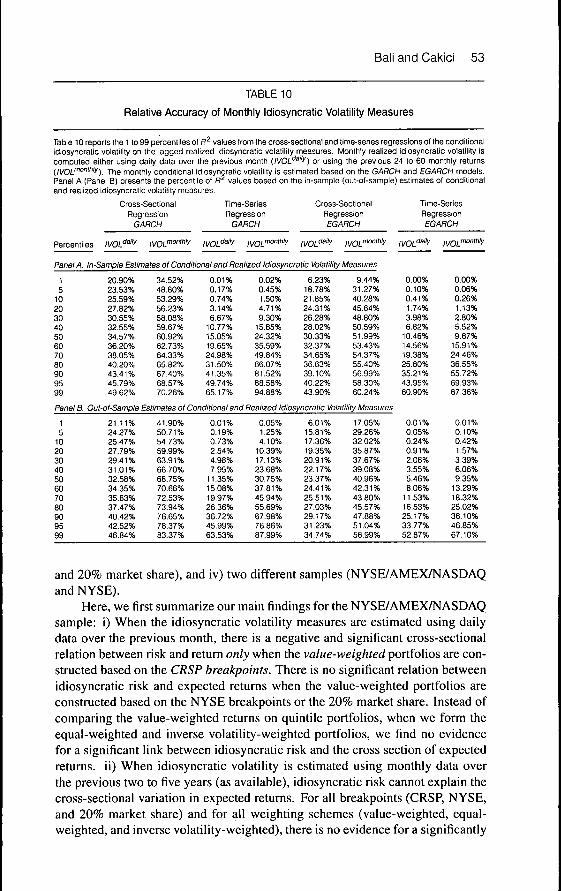
Bali and Cakici 53
TABLE 10
Relative Accuracy of Monthly Idiosyncratic Volatility Measures
Table 10 reports the 1 to 99 percentiles of R^ values from the oross-sectional and time-series regressions of the conditionalidiosyncratic voiatiiity on the iagged reaiized idiosynoratio voiatiiity rneasures. f^onthly realized idiosyncratic voiatiiity isoompijted either using daily data over the previous month {iVOL^^'^^) or using the previous 24 to 60 monthly returns(/l/OL'""""''''). The monthly conditional idiosynoratio volatility is estimated based on the GARCH and EGARCH modeis.Panei A (Panei B) presents the percentiie of R^ vaiues based on the in-sample (out-of-sample) estimates of conditionaland realized idiosyncratic voiatiiity measures.
Percentiies
Cross-SecticnaiRegression
GARCH
ivof-'y
Time-SeriesRegression
GARCH
ivof-'y
Cross-SectionalRegressionEGARCH
iVOL^^'^y
Panei A. in-Sampie Estimates of Conditionai and Reaiized Idiosyncratic Voiatiiity Measures
15
1020304050607080909599
20.90%23.53%25.59%27.82%30.55%32.55%34.57%36.20%38.05%40.20%43.41%45.79%49.62%
34.52%48.80%53.29%56.23%58.08%59.67%60.92%62.73%64.33%65.82%67.40%68.57%70.26%
0.01%0.17%0.74%3.14%6.67%
10.77%15.05%19.65%24.98%31.50%41.35%49.74%65.17%
0.02%0.45%1.50%4.71%9.30%
15.85%24.32%35.59%49.84%66.07%81.52%88.58%94.88%
6.23%18.78%21.85%24.31%26.28%28.02%30.33%32.37%34.65%36.63%39.10%40.22%43.90%
9.44%31.27%40.28%45.64%48.80%50.59%51.99%53.43%54.37%55.40%56.99%58.30%60.24%
Time-SeriesRegressionEGARCH
ivof-'y
0.00%0.10%0.41%1.74%3.98%6.82%
10.46%14.56%19.38%25.80%35.21%43.95%60.90%
Panei B. Out-of-Sampie Estimates of Conditionai and Reaiized idiosyncratic Voiatiiity Measures
15
1020304050607080909599
21.11%24.27%25.47%27.79%29.41%31.01%32.58%34.35%35.83%37.47%40.42%42.52%46.84%
41.90%50.71%54.73%59.99%63.91%66.70%68.75%70.66%72.53%73.94%76.65%78.37%83.37%
0.01%0.19%0.73%2.54%4.98%7.95%
11.35%15.08%19.97%26.36%36.72%45.99%63.53%
0.05%1.25%4.10%
10.39%17.13%23.68%30.75%37.81%45.94%55.69%67.98%76.86%87.99%
6.01%15.81%17.36%19.35%20.91%22.17%23.37%24.41%25.51%27.03%29.17%31.23%34.74%
17.05%29.26%32.02%35.87%37.67%39.08%40.96%42.31%43.80%45.57%47.88%51.04%56.99%
0.01%0.05%0.24%0.91%2.06%3.55%5.46%8.06%
11.53%16.53%25.17%33.77%52.87%
0.00%0.06%0.26%1.13%2.80%5.52%9.67%
15.91%24.46%36.55%55.72%69.93%87.36%
0.01%0.10%0.42%1.57%3.39%6.06%9.35%
13.29%18.32%25.02%36.10%46.85%67.10%
and 20% market share), and iv) two different samples (NYSE/AMEX/NASDAQand NYSE).
Here, we first summarize our main findings for the NYSE/AMEX/NASDAQsample: i) When the idiosyncratic volatility measures are estimated using dailydata over the previous month, there is a negative and significant cross-sectionalrelation between risk and return only when the value-weighted portfolios are con-structed based on the CRSP breakpoints. There is no significant relation betweenidiosyncratic risk and expected returns when the value-weighted portfolios areconstructed based on the NYSE breakpoints or the 20% market share. Instead ofcomparing the value-weighted returns on quintile portfolios, when we form theequal-weighted and inverse volatility-weighted portfolios, we find no evidencefor a significant link between idiosyncratic risk and the cross section of expectedreturns, ii) When idiosyncratic volatility is estimated using monthly data overthe previous two to five years (as available), idiosyncratic risk cannot explain thecross-sectional variation in expected returns. For all breakpoints (CRSP, NYSE,and 20% market share) and for all weighting schemes (value-weighted, equal-weighted, and inverse volatility-weighted), there is no evidence for a significantly
54 Journal of Financial and Quantitative Analysis
positive or negative average return differential on the lowest volatility and highestvolatility portfolios, iii) If we rely on the differences in FF-3 alphas, we find asignificantly negative relation only for the value-weighted portfolios with CRSPbreakpoints. However, for the equal-weighted and inverse volatility-weightedportfolios and for the breakpoints of NYSE and 20% market share, the link be-tween idiosyncratic volatility and expected returns is economically and statisti-cally insignificant.
The results from the NYSE sample indicate that there is no robust evidencefor a significant relation between idiosyncratic risk and the cross section of ex-pected returns. For all idiosyncratic volatility measures (estimated using bothdaily and monthly data), for both the NYSE breakpoints and the 20% marketshare, and for both the value-weighted and the equal-weighted portfolios, the av-erage return differential on the lowest and highest idiosyncratic volatility portfo-lios is very small and statistically insignificant. If we rely on the differences inFF-3 alphas, we find a negative and significant relation when idiosyncratic volatil-ity is estimated using the daily data. However, such a relation disappears whenthe monthly data are used to compute idiosyncratic volatility.
To check whether small and illiquid stocks are driving the results of AHXZ(2006), we use a sample of NYSE/AMEX/NASDAQ stocks that involves a screenfor size, price, and liquidity. After excluding the smallest, lowest priced, andleast liquid stocks in the NYSE/AMEX/NASDAQ sample, we find a negative andsignificant relation between idiosyncratic risk and the cross section of expectedreturns on small stock portfolios. However, such a relation does not exist forlarge stock portfolios because the 5-1 differences in average returns and FF-3alphas are small and statistically insignificant. Alternatively, we generate threesubsamples for i) large/liquid, ii) large/high price, and iii) liquid/high price stocks.After eliminating the smallest and least liquid; the smallest and lowest priced; andthe least liquid and lowest priced stocks in the NYSE/AMEX/NASDAQ sample,there is no robustly significant link between idiosyncratic volatility and expectedstock returns.
We use two different measures of monthly idiosyncratic volatility in ourcross-sectional tests. The key difference between these two measures {lVOL''''''^versus IVOL"'""''''^) is that for some portfolios there is a significantly negative re-lation between IVOL''""^ and the cross section of expected returns, whereas thecross-sectional relation between IVOL'""""''^ and expected stock returns is fiator very weak. To determine if there is a significant link between idiosyncraticrisk and expected returns, we compare the relative accuracy of IVOL'''''''' andjyQjmonthiy jj^g statistical results indicate that the ivOL""""'''y provides a bet-ter characterization of expected future volatility than the lVOL''''"y, which leadsus to safely conclude that the negative trade-off between risk and return does notexist.
Appendix. Value-Weighted versus Equal-Weighted Portfolios
Table Al shows that when monthly idiosyncratic volatility is estimated using dailydata and when the NYSE/AMEX/NASDAQ stocks are sorted based on the CRSP break-
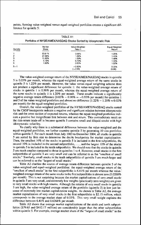
Bali and Cakici 55
points, forming value-weighted versu,s equal-weighted portfolios creates a significant dif-ference for quintile 5:
TABLE Al
Portfolios of NYSE/AMEX/NASDAQ Stocks Sorted by Idiosyncratic Risk
Ouintile
12345
5-i'
MarketShare
53.81%27.26%11.82%5.18%1.92%
Value-WeightedReturn
0.96%1.06%1.09%0.73%0.03%
-0.93%(-2.68)
Equal-WeightedReturn
1.20%1.45%1.48%1.33%1.22%
0.02%(0.06)
The value-weighted average return of the NYSE/AMEX/NASDAQ stocks in quintile5 is 0,03% per month, whereas the equal-weighted average return of the same stocks inquintile 5 is 1,22% per month. However, the value versus equal weighting scheme doesnot produce a significant difference for quintile 1: the value-weighted average return ofstocks in quintile 1 is 0,96% per month, whereas the equal-weighted average return ofthe same stocks in quintile 1 is 1,20% per month. These results indicate a significantlynegative average return difference (0,03% - 0,96% = -0,93% per month) for quintiles 1and 5 of the value-weighted portfolios and almost no difference (1,22% — 1,20% = 0,02%per month) for the equal-weighted portfolios.
Overall, the value-weighted portfolios of the NYSE/AMEX/NASDAQ stocks sortedby the CRSP breakpoints indicate a negative and significant relation between idiosyncraticrisk and the cross section of expected returns, whereas the equal-weighted portfolios indi-cate a positive but insignificant link between risk and return. This contradictory result onthe risk-return trade-off is because quintile 5 contains small and illiquid stocks with highidiosyncratic volatility.
To clarify why there is a substantial difference between the value-weighted and theequal-weighted portfolios, we further examine quintile 5 by generating 10 size portfolioswithin quintile 5, For each month from July 1963 to December 2004, all stocks in quintile5 are sorted by firm size to determine the decile breakpoints for market capitalization.Then, the smallest 10% of the stocks in quintile 5 is included in the first subportfolio, thesecond 10% is included in the second subportfolio, , , , , and the largest 10% of the stocksin quintile 5 is included in the tenth subportfolio. We should note that the stocks in quintile5 are much smaller compared to those in quintiles 1 to 4, However, small stocks in the firstsubportfolio of quintile 5 are very small and can be referred to as the "smallest of smallstocks," Similarly, small stocks in the tenth subportfolio of quintile 5 are much larger andcan be referred to as the "largest of small stocks,"
Table A2 clarifies the source of average return difference between quintile 5 of thevalue-weighted and equal-weighted portfolios: the equal-weighted average return of the"smallest of small stocks" in the first subportfolio is 6,41% per month whereas the value-^weighted average return of the same stocks in the first subportfolio is almost zero (0,0268%per month). This is not surprising because the market capitalizations of very small stocksin quintile 5 are very small, and extremely low weights (practically zero weights) are givento very small stocks with high returns. Although the returns of very small stocks in quintile5 are high, the value-weighted average return of the portfolio (quintile 5) is low just be-cause of extremely low market capitalization weights. As shown in Table A2, the averagemarket capitalization of very small stocks in the first subportfolio is $2,15 million, whichcorresponds to the average market share of 0,55%, This very small weight explains thedifference between 6,41% and 0,0268% per month.
Table A2 shows that average market capitalizations of the ninth and tenth subport-folios ($79,65 and $412,17 million) are considerably larger than the other subportfolioswithin quintile 5, For example, average market share of the "largest of small stocks" in the
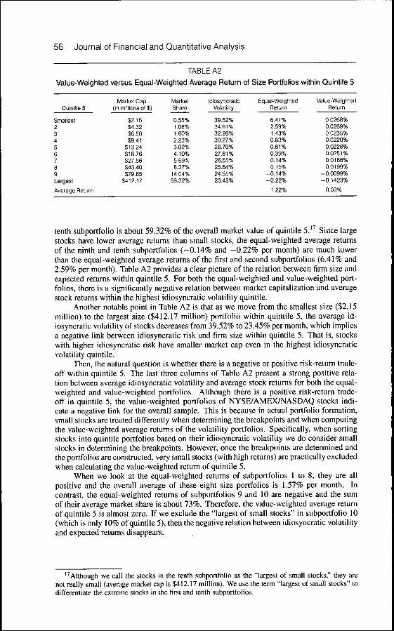
56 Journal of Financial and Quantitative Analysis
TABLE A2
Value-Weighted versus Equal-Weighted Average Return
Quintile 5
Smailest23456789Largest
Average Return
Market Cap(in miliions of $)
$2.15$4.32$6.56$9.41
$13.24$18.76$27.56$43.40$79.65
$412.17
MarketShare
0.55%1.08%1.60%2.23%3.02%4.10%5.69%8.37%
14.04%59.32%
idiosyncraticVolatility
39.52%34.61%32.26%30.27%28.70%27.81%26.55%25.84%24.55%23.45%
of Size Portfolios
Equal-WeightedReturn
6.41%2.59%1.43%0.83%0.61%0.39%0.14%0.15%
-0.14%-0.22%
1.22%
within Quintile 5
Vaiue-WeiQhtedReturn
0.0268%0.0269%0.0235%0.0220%0.0228%0.0251%0.0166%0.0199%
-0.0099%-0.1423%
0.03%
tenth subportfolio is about 59.32% of the overall market value of quintile 5.'^ Since largestocks have lower average returns than small stocks, the equal-weighted average returnsof the ninth and tenth subportfolios (—0.14% and —0.22% per month) are much lowerthan the equal-weighted average returns ofthe first and second subportfolios (6.41% and2.59% per month). Table A2 provides a clear picture of the relation between firm size andexpected returns within quintile 5. For both the equal-weighted and value-weighted port-folios, there is a significantly negative relation between market capitalization and averagestock returns within the highest idiosyncratic volatility quintile.
Another notable point in Table A2 is that as we move from the smallest size ($2.15million) to the largest size ($412.17 million) portfolio within quintile 5, the average id-iosyncratic volatility of stocks decreases from 39.52% to 23.45% per month, which impliesa negative link between idiosyncratic risk and firm size within quintile 5. That is, stockswith higher idiosyncratic risk have smaller market cap even in the highest idiosyncraticvolatility quintile.
Then, the natural question is whether there is a negative or positive risk-return trade-off within quintile 5. The last three columns of Table A2 present a strong positive rela-tion between average idiosyncratic volatility and average stoek returns for both the equal-weighted and value-weighted portfolios. Although there is a positive risk-return trade-off in quintile 5, the value-weighted portfolios of NYSE/AMEX/NASDAQ stocks indi-cate a negative link for the overall sample. This is because in actual portfolio formation,small stocks are treated differently when determining the breakpoints and when computingthe value-weighted average returns of the volatility portfolios. Specifically, when sortingstocks into quintile portfolios based on their idiosyncratic volatility we do consider smallstocks in determining the breakpoints. However, once the breakpoints are determined andthe portfolios are constructed, very small stocks (with high returns) are practically excludedwhen calculating the value-weighted return of quintile 5.
When we look at the equal-weighted returns of subportfolios 1 to 8, they are allpositive and the overall average of these eight size portfolios is 1.57% per month. Incontrast, the equal-weighted returns of subportfolios 9 and 10 are negative and the sumof their average market share is about 73%. Therefore, the value-weighted average returnof quintile 5 is almost zero. If we exclude the "largest of small stocks" in subportfolio 10(which is only 10% of quintile 5), then the negative relation between idiosyncratic volatilityand expected returns disappears.
'^Although we call the stocks in the tenth subportfolio as the "largest of small stocks," they arenot really small (average market cap is $412.17 million). We use the term "largest of small stocks" todifferentiate the extreme stocks in the first and tenth subportfolios.
Bali and Cakici 57
References
Amihud, Y. "Illiquidity and Stock Returns: Cross-Section and Time-Series Effects." Journal ofFinancial Markets, 5 (2002), 31-56.
Ang, A.; R. J. Hodrick; Y. Xing; and X. Zhang. "The Cross-Section of Volatility and ExpectedReturns." Journal of Finance. 61 (2006), 259-299.
Bali, T. G. 'Testing the Empirical Performance of Stochastic Volatility Models of the Short-TermInterest Rate." Journal of Financial and Quanlitalive Analysis, 35 (2000), 191-215.
Bali, T G.; N. Cakici; X. Yan; and Z. Zhang. "Does Idiosyncratic Risk Really Matter?" Journal ofFinance, 60 (2005), 905-929.
Bessembinder, H. "Systematic Risk, Hedging Pressure, and Risk Premiums in Futures Markets."Review of Financial Studies, 5 (1992), 637-667.
Black. F. "Capital Market Equilibrium with Restricted Borrowing." Journal of Business, 45 (1972),444-^55.
Bollerslev, T. "Generalized Autoregressive Conditional Heteroscedasticity." Journal of Econometrics,31 (1986), 307-327.
Campbell, J. Y.; M. Lettau; B. G. Malkiel; and Y. Xu. "Have Individual Stocks Become More Volatile?An Empirical Exploration of Idiosyncratic Risk." Journal of Finance, 56 (2001), 1-43.
Cohen, R. B., and C. K. Polk. "The Impact of Industry Factors in Asset-Pricing Tests." WorkingPaper, Harvard University (1998).
Douglas, G. W. "Risk in the Equity Markets: An Empirical Appraisal of Market Efficiency." YaleEconomic Essays, 9 (1969), 3-45.
Falkenstein, E. G. "Preferences for Stock Characteristics as Revealed by Mutual Fund Portfolio Hold-ings." Journal of Finance, 51 (1996), 111-135.
Fama. E. F, and K. French. "Cross-Section of Expected Stock Returns." Journal of Finance, 47(1992), 427^65.
Fama, E. F., and K. French. "Common Risk Factors in the Returns on Stocks and Bonds." Journal ofFinancial Economics, 33 (1993), 3-56.
Fama. E. F, and J. D. MacBeth. "Risk and Return: Some Empirical Tests." Journal of PoliticalEconomy, 81 (1973), 607-636.
Fu, F, "Idiosyncratic Risk and the Cross-Section of Expected Stock Returns." Working Paper, Uni-versity of Rochester (2005).
Green, R. C, and K. Rydqvist. "The Valuation of Nonsystematic Risks and the Pricing of SwedishLottery Bonds." Review of Financial Studies, 10 (1997), 447-480.
Harris, L. E. "Minimum Price Variation, Discrete Bid-Ask Spreads, and Quotation Sizes." Review ofFinancial Studies, 7 (1994), 149-178.
Jegadeesh, N., and S. Titman. "Profitability of Momentum Strategies: An Evaluation of AlternativeExplanations." Journal of Finance, 56 (2001), 699-720.
Jones, C. M., and M. Rhodes-Kropf. "The Price of Diversifiable Risk in Venture Capital and PrivateEquity." Working Paper, Columbia University (2003).
King, M.; E. Sentana; and S. Wadhwani. "Volatility and Links between National Stock Markets."Econometrica, 47 (1994), 263-291.
Kyle, A. "Continuous Auctions and Insider Trading." Econometrica, 53 (1985), 1315-1335.Lehmann, B. N. "Residual Risk Revisited." Journal of Econometrics, 45 (1990), 71-97.Levy, H. "Equilibrium in an Imperfect Market: A Constraint on the Number of Securities in the
Portfolio." American Economic Review, 68 (1978), 643-658.Lintner, J. "The Valuation of Risky Assets and the Selection of Risky Investments in Stock Portfolios
and Capital Budgets." Review of Economics and Statistics, 47 (1965a), 13-37.Lintner, J. "Security Prices, Risk and Maximal Gains from Diversification." Journal of Finance, 20
(1965b), 587-615.Malkiel, B. G., and Y. Xu. "Risk and Return Revisited." Journal of Portfolio Management, 24 (1997),
9-14.Malkiel, B. G., and Y. Xu. "Idiosyncratic Risk and Security Returns." Working Paper, University of
Texas at Dallas (2002).Markowitz, H. Portfolio Selection: Efficient Diversification of Investments. New York: Wiley (1959).Merton, R. C. "A Simple Model of Capital Market Equilibrium with Incomplete Information." Journal
of Finance, 42 (1987), 483-510.Miller, M. H., and M. Scholes. "Rates of Return in Relation to Risk: A Re-Examination of Some
Recent Findings." In Studies in tbe Theory of Capital Markets, M. C. Jensen, ed. New York:Praeger(I972).
Nelson, D. B. "Conditional Heteroskedasticity in Asset Returns: A New Approach." Econometrica,59(1991), 347-370.
58 Journal of Financial and Quantitative Analysis
Newey, W. K., and K. D. West. "A Simple, Positive Semi-Definite, Heteroskedasticity and Autocor-relation Consistent Covariance Matrix." Econometrica, 55 (1987), 703-708.
Sharpe, W. F. "Capital Asset Prices: A Theory of Market Equilibrium under Conditions of Risk."Joumal of Finance, 19 (1964), 425-442.
Spiegel, M., and X. Wang. "Cross-Sectional Variation in Stock Returns: Liquidity and IdiosyncraticRisk." Working Paper No. 05-13, Yale ICF (2005).
Tinic, S. M., and R. R. West. "Risk, Return and Equilibrium: A Revisit." Joumal of Political Econ-om3;,94(1986), 126-147.
Xu, Y., and B. G. Malkiel. "Investigating the Behavior of Idiosyncratic Volatility." Joumal ofBusi-/i£ii, 76(2003), 613-644.