The Regional Economics Applications Laboratory (REAL) is a cooperative venture be-tween the University of Illinois and the Federal Reserve Bank of Chicago focusing on the development and use of analytical models for urban and regional economic development. The purpose of the Discussion Papers is to circulate intermediate and final results of this research among readers within and outside REAL. The opinions and conclusions ex-pressed in the papers are those of the authors and do not necessarily represent those of the Federal Reserve Bank of Chicago, Federal Reserve Board of Governors or the University of Illinois. All requests and comments should be directed to Geoffrey J. D. Hewings, Director, Regional Economics Applications Laboratory, 607 South Matthews, Urbana, IL, 61801-3671, phone (217) 333-4740, FAX (217) 244-9339. Web page: www.uiuc.edu/unit/real

SPATIAL EVIDENCE OF AGGLOMERATION ECONOMIES IN CHICAGO

Jungyul Sohn and Geoffrey J.D. Hewings

REAL 00-T-4 May, 2000

Spatial Evidence of Agglomeration Economies in Chicago

Jungyul Sohn and Geoffrey J.D. Hewings Department of Geography, University of Illinois, Urbana, USA

Abstract: Agglomeration economies feature prominently in the analysis of differences in urban economic structure across urban areas. While agglomeration economies between cities focus at the macro-scale of analysis, such economies within any given city focus more on the micro geographical scale. There have been a number of researches on agglomeration economies, among which there are relatively few approaches based on intraurban context. This paper explores agglomeration at the micro scale and tries to reveal the spatial realization of agglomeration economies within and between sectors. The study area is the Chicago CMSA; 306 zip code zones and three sectors are considered; manufacturing, retail and service. The model is based on simultaneous equation systems and 2SLS and KRP estimators. The result shows that there are positive simultaneous relationships between manufacturing and retail and also between retail and service while service has a negative endogenous influence on manufacturing. The growth of retail and service attracts more of the same kind of activities. Related to the previous economic environment, manufacturing dominant areas are not preferable places for retail firms to locate and vice versa; however, these areas are attractive ones for service firms. Manufacturing and retail firms prefer to choose to locate in areas with higher levels of manufacturing and retail activities respectively while service firms do the opposite. The traditional “jobs follow people” hypothesis is not observed to be significant in this analysis.

1. Introduction As Fujita and Thisse (1996) noted, agglomeration economies can be identified at different geographical scales; for example, similar activities clustered within the same neighborhood of a city at the one extreme to the core-periphery structure of international inequality problems at the other extreme. While more researches have been focused on the latter, relatively fewer empirical researches have been performed on the first category. The basic issue addressed in this paper is whether agglomeration economies operating at the metropolitan level as a unit are also in evidence within cities. Since the classic research of Alonso (1964), urban spatial structure has been a major focus of research. While the term ‘urban spatial structure’ may be used in different contexts, it generally entails urban economic spatial structure and urban residential spatial structure. Those two are, without doubt, the main activities or functions in most urban places. Spatial structure is realized by the spatial distribution pattern as well as its change over time. If the focus is more on the disaggregated level of activities and functions, for example, down to individual firms and households, then the distribution pattern splits into individual location/relocation decisions. Earlier models more often adapted single equation systems to explain the variations in the distribution and/or location patterns of a certain activity in an urban space. For example, if the dependent variable is set up as the level of economic activities in a certain zone, residence in that zone is used as an exogenous variable and vice versa. In this type of model specification, it should always be assumed that the latter cause the former, but not vice versa. In this sense, the model provides a more limited and controlled environment to handle reality; interactions between economic activities and residences are not properly considered in the model while the real world suggests a synergetic relationship. As a result of this limitation, more efforts in the last two or three decades have been directed to analysis of the simultaneity of urban activities; the most prevailing model for this purpose has been simultaneous equation systems. By adapting this framework,

2

researchers were able to handle causality from both sides of the activity at once. While there were many differences in detail among the models, the general consensus revealed a causal relationship from residences to economic activities but not in the other direction. For example, jobs (firms) follow people but people don’t follow jobs (firms).1 A more detailed review of their research will be provided in the next section. While there has been a great deal of attention focused on interrelation between economic activities and residences, it is hard to find research examining interactions among different industrial sectors in the economy. As mentioned above, the distribution or location pattern of a single firm or a group of firms in a certain sector is affected by the pattern of residents. Similarly, one might expect that the distribution and location pattern of firms in other sectors also has an influence on the distribution or location decision of a certain firm. Generally speaking, firms show some level of attraction to the same kind of or other firms with varying degrees. The explanation for these phenomena is rooted in the concept of external economies or agglomeration economies.2 Firms seem to be better off when they are spatially aggregated than when they are dispersed. This is especially the case when functional specialization between firms exists and geographic closeness matters. 3 Two perspectives can be adopted to explore the role of agglomeration economies, although they are not strictly exclusive. The intra-industry perspective, locating near firms in the same industry, provides the industrial firm with great access to more relevant infrastructure. The inter-industry perspective, locating near those firms in other economic sectors, offers the firm direct access to sources of backward and/or forward linkages. According to more popular typology of agglomeration economies among urban economic literatures, the former is termed as localization economies whereas the latter as urbanization economies. (e.g. Pascal and McCall (1980), Goldstein and Gronberg (1984), Nakamura (1985), Fogarty and Garofalo (1988) and McMillen and McDonald (1998)4) While the effect of those two economies may not be clearly divided, Fogarty and Garofalo (1988) adopted the function of the scale of the manufacturing sector (returns-to-scale) as the estimate of localization economy and the function of urban scale (efficiency parameter of the production function) as the estimate of urbanization economy in the model. They showed localization factors were significant in explaining productivity at the SMSA level. But they suggested that urbanization economy might not be solely significant and rather urban spatial structure or arrangement of economic activity also needed to be considered in the model. With more disaggregate sectoral classification of manufacturing, Nakamura (1985) concluded that light manufacturing industries were more influenced by urbanization economies and heavy manufacturing industries more by localization economies in his research focusing on Japanese cities.

1 See Steinnes (1977), Greenwood (1980), Boarnet (1994a; 1994b) and Deitz (1998) for more detailed discussion on this proposition. 2 The concept of increasing returns to scale provides a starting point of economic process of agglomeration economies. For the extensive review of the literatures on this topic, refer to Fujita and Thisse (1996). 3 The terms, “functional specialization” and “geographic closeness” were two dimensions to explain the level of agglomeration economies in the paper of Bergsman, Greenston and Healy (1975). 4 Some authors did not explicitly use those terms to present the characteristics of those two economies (e.g. Pascal and McCall (1980) and McMillen and McDonald (1998)) or had more than two types of economies classified. (e.g. Pascal and McCall (1980) and Goldstein and Gronberg (1984)) But the fundamental idea behind those is still under the general classification scheme of localization and urbanization economies.

3

Many of theoretical and empirical researches on agglomeration economies have explored the relationship between agglomeration economy and other urban and economic features. Abdel-Rahman (1990) developed a theoretical framework to examine the different size and type of cities associated with dominant agglomeration forces between cities. He argued that industrial structure within the city or spatial proximity between related industries was an important factor in explaining the differences. With the empirical model, Mitra (1999) also focused on city size issue. Comparing city size and agglomeration economies measured as technical efficiency, he concluded that those two had positive relationship even if diseconomies of scale would be realized over a certain threshold level of city size. Researches with focus on the relationship between agglomeration and other factors include the ones on technical change and agglomeration economy (Calem and Carlino, 1991), on urban capital market and agglomeration economy (Helsley and Strange, 1991), and on land rents and wages and agglomeration economies (Dekle and Eaton, 1999). While many authors linked agglomeration economies with economies of scale, Goldstein and Gronberg (1984) attempted to explain the feature with the economies of scope that is realized as vertical integration process of production. Unlike most others who focused on manufacturing activity, Mun and Hutchinson (1995) extended the scope of the subject. In a case study of Toronto, they distinguished their research from the general stream of prior research in that it focused on intra-urban locations, in terms of the geographical scale, and on the office sector, as opposed to manufacturing. However, the existence of probable external economies between industries remains unexplored. Another group of researches have shown more explicit interest in spatial context of those agglomeration economies. Lee (1981) adopted a standard distance measure from the economically weighted centroid to individual firms in each sector and contiguity measures as well to check the level of agglomeration economies or spatial concentration of individual industries. Since the measures were limited to consideration of firms in the same sector, the scope of research was confined to exploring the level of intra-industry agglomeration economies. Maurel and Sedillot’s (1999) paper was one of the few that dealt with intra- and inter-industry relations at the same time. Based on previous researches, they derived several indices measuring the level of geographic concentration; these indices were interpreted as the correlation between the location decisions of two firms. By applying them to french manufacturing industries, the authors sought to identify the spatial realization of agglomeration economies. While those indices are useful to check the overall pattern of spatial distribution, causality between industries with respect to the distribution may not be identified. Hanson (1996) proved in his empirical research that spatial economic pattern experiences iterative process of agglomeration, dispersion and reagglomeration due to the changing role of external economies and diseconomies. Dekle and Eaton (1999) explored the distance decay effect of agglomeration economies and concluded that the financial sector was more sensitive to the effect than the manufacturing and as a result had less geographical reach of spillover. For some, agglomeration economies are not the only answer for the questions on economic and urban growth. DeCoster and Strange (1993) used the term ‘spurious agglomeration’ to represent the situation in which excessive concentration of economic activity occurs due to incentive programs. They noted that the system would be inefficient and could be relieved by a certain tax measure. Both Moomaw (1985) and

4

Hanson (1990) uncovered the contemporary economy was in transition from the stage that favored agglomeration economies to another. Moomaw (1985) showed the productivity advantages of large cities have declined in eight 2-digit manufacturing sectors accounting for more than one third of production worker employment. Hanson (1990) proposed that productivity advantage of the center was offset by the higher land and labor cost and the result suggested market forces might lead eventually to decentralization of industries. Smith and Florida (1994) also mentioned that there also seemed to be conflicting effects of agglomeration economies and those on the negative side (diseconomies) included higher factor costs resulting from locations in brown-field sites, higher wages, higher levels of unionization, and greater social problems. In his probit model to test firms’ location behavior, Cooke (1983) showed that traditional measures of agglomeration economies such as proximities to backward and forward linkage activities were lack of explanatory power. Rather, as he noted, demand changes, initial plant size or relative magnitude transport cost has gained more importance. The purpose of this paper is to examine the spatial realization of agglomeration economies in Chicago in the 1990s. More specifically, it focuses on the interrelated influence of the spatial distribution pattern of each sector of the economy on the other sectors. To investigate the relative significance of agglomeration economies, the model also incorporates several residential factors. In the next section, a brief review of prior analysis is provided, especially focusing on the simultaneous relationship between urban activities. Section 3 and 4 define the model used in the analysis and the estimation methods; the model is a spatial econometric simultaneous equation system. Section 5 provides the estimated results and interpretations. Finally, section 6 summarizes the analysis and indicates some remaining, unresolved issues.

2. Simultaneity of Urban Activities From Alonso’s (1964) pioneering analysis of internal urban structure, the work of Moses and Williamson (1972) explored manufacturing location and relocation behavior in Chicago; they decomposed the analysis into three parts along with the location and relocation process: distribution of origin, distance of movement and destination analysis. By so doing, the authors tried to explore the decentralization process. Since a single regression model approach was adopted, limited explanation could be offered on the interrelated characteristics of urban spatial structure. Since the late 1970s, simultaneous specification of the urban spatial structure has been featured more prominently. Much of the interest lay in the causality between jobs and residences in terms of the spatial location and/or relocation pattern. While it is hard to generalize the results of all relevant researches, more of them have shared the conclusion that jobs follow people. Cooke (1978) was one of the earliest scholars who explored the causality between residence and employment. Based on the Steinnes model, he refined a simultaneous model that incorporated sectoral (manufacturing, retail and service) as well as residential density gradients as endogenous variables. The conclusion confirmed that jobs follow people. Greenwood (1980) showed a similar interest in the urban spatial structure. While his major focus was on the relationship between people and jobs, part of his simultaneous model was devoted to explaining the distribution of 4 economic sectors

5

– manufacturing, retail, wholesale and service. Although he used some sectors (such as manufacturing and retail) as independent variables in the regression for another sectors (such as wholesale and service), no simultaneous relationship between sectors was explored, although he did note that those sector variables were significant in the model. He also confirmed the finding that jobs followed people. A series of studies by Boarnet (1994a; 1994b) in the 1990s developed a more extended scope of simultaneous equation models that were able to incorporate the spatial effects between and within variables. By analyzing 365 municipalities in New Jersey, he confirmed the results of many previous analyses – jobs follow people. While he included various spatial lag variables, incorporating spatial lag for the dependent variable (i.e., spatial autoregressive simultaneity, see Rey and Boarnet, 1998, p.8) could be another alternative. Deitz (1998) derived the model in a similar fashion to Boarnet in that he started with the equilibrium distribution of urban economic activities and population and applied spatial effect variables as a measure of accessibility. While Boarnet used the change of employment and residence between years as endogenous variables, Deitz adopted employment and residence in the latter year of the two as endogenous. He also considered cross relationship between different sectors: for example, a variable of workers in one sector is included in the equation to explain the employment in another sector. Using 2SLS estimators on 438 Boston MSA census tract data, he also concluded that jobs follow people. While many researches have proved the causal effect of residence on employment, there are several other researches that drew different conclusions. As an extension of the Alonso-Muth framework, Siegel (1975) developed a model that allows the household to simultaneously choose its residential and employment location and some other features in order to maximize its utility subject to the budget constraint. Among others, one result showed that residence and employment locations are responsive to each other. A similar result was found in Grubb (1982). He explained the logic behind the behavior of being close to other activities. For example, firms like to be near people not only as potential customers but also as a source of factor inputs. Residents also like to move closer to economic activities, both for employment opportunities as well as for shopping activities. Starting with the similarly specified model, Grubb (1982) drew a similar conclusion; that is, jobs followed people and people followed jobs. He also revealed that there is a self-reinforcing effect between certain economic sectors in their location/relocation. In a rather different context, Ommeren, Rietveld and Nijkamp (1999) have sought the answers for the similar question. Instead of focusing on the overall distribution pattern of economic activities and residences, they examined the location/relocation factors for people to move their jobs and residences. However, unlike many of the conclusions drawn from a more aggregated studies, they suggested that there is no evidence that job and residential moves are mutually related. And the structural simultaneous probit model confirmed this proposition again. Some researches were more specific in determining the causal relationship between residence and employment location rather than providing a single generalized conclusion. For example, Steinnes (1977) set up a dynamic model using pooled cross-sectional time-series data not only on the level of activities at a certain time but also on the change of those activities in an attempt to examine the relationship between residences and economic activities. He concluded that jobs followed people especially in manufacturing

6

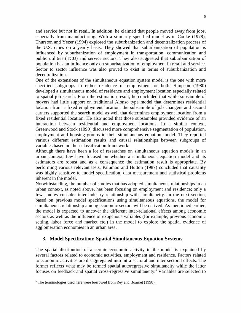
and service but not in retail. In addition, he claimed that people moved away from jobs, especially from manufacturing. With a similarly specified model as in Cooke (1978), Thurston and Yezer (1994) explored the suburbanization and decentralization process of the U.S. cities on a yearly basis. They showed that suburbanization of population is influenced by suburbanization of employment in transportation, communication and public utilities (TCU) and service sectors. They also suggested that suburbanization of population has an influence only on suburbanization of employment in retail and service. Sector to sector influence was also proved to exist in terms of suburbanization and decentralization. One of the extensions of the simultaneous equation system model is the one with more specified subgroups in either residence or employment or both. Simpson (1980) developed a simultaneous model of residence and employment location especially related to spatial job search. From the estimation result, he concluded that while subsample of movers had little support on traditional Alonso type model that determines residential location from a fixed employment location, the subsample of job changers and second earners supported the search model as well that determines employment location from a fixed residential location. He also noted that those subsamples provided evidence of an interaction between residential and employment locations. In a similar context, Greenwood and Stock (1990) discussed more comprehensive segmentation of population, employment and housing groups in their simultaneous equation model. They reported various different estimation results and causal relationships between subgroups of variables based on their classification framework. Although there have been a lot of researches on simultaneous equation models in an urban context, few have focused on whether a simultaneous equation model and its estimators are robust and as a consequence the estimation result is appropriate. By performing various relevant tests, Palumbo and Hutton (1987) concluded that causality was highly sensitive to model specification, data measurement and statistical problems inherent in the model. Notwithstanding, the number of studies that has adopted simultaneous relationships in an urban context, as noted above, has been focusing on employment and residence; only a few studies consider inter-industry relationship with simultaneity. In the next section, based on previous model specifications using simultaneous equations, the model for simultaneous relationship among economic sectors will be derived. As mentioned earlier, the model is expected to uncover the different inter-relational effects among economic sectors as well as the influence of exogenous variables (for example, previous economic setting, labor force and market etc.) in the model to explore the spatial evidence of agglomeration economies in an urban area.

3. Model Specification: Spatial Simultaneous Equation Systems The spatial distribution of a certain economic activity in the model is explained by several factors related to economic activities, employment and residence. Factors related to economic activities are disaggregated into intra-sectoral and inter-sectoral effects. The former reflects what may be termed spatial autoregressive simultaneity while the latter focuses on feedback and spatial cross-regressive simultaneity.5 Variables are selected to 5 The terminologies used here were borrowed from Rey and Boarnet (1998).

7

explain the different aspects of agglomeration economies within and between sectors. Factors related to residence are population in general and employees in a specific economic sector. While the former is seen as proxy for market potential for firms, the latter is considered labor pool of a specific industry. Generally, larger population leads to higher level of demands on goods and services. Firms may prefer staying close to areas with higher demands to maintain higher market share by reducing transportation cost (and as a result, reducing market price of goods and services). In a similar fashion, larger labor pool leads to higher level of cheap labor supply. Cheaper supply of labor enables firms to lower production costs and as a result the market price of those goods and services. In this sense, those two are expected to work as centripetal forces to certain zones. Equation (1) through (3) yield the equilibrium condition of the simultaneity for three economic sectors. As Anselin and Bera (1998, p.247) noted, when data are based on administratively determined units, there is no good reason to expect economic behavior to conform to these units. As a consequence, it might be reasonable to use variables with spatial weight (W) attached on them to bridge the gap between the two as the model below shows.

8

If we assume the function is linear and equilibrium is reached at time t, the following equations hold for the system.

izonearoundandinpopulationtotaloflevelPOPWIizonearoundandinemployeesservicenonoflevelEMPWI

izonearoundandinemployeesretailnonoflevelEMPWIizonearoundandinemployeesingmanufacturnonoflevelEMPWI

izonearoundandinemployeesserviceoflevelEMPWIizonearoundandinemployeesretailoflevelEMPWI

izonearoundandinemployeesingmanufacturoflevelEMPWIcetandisbyewightedizonearoundfirmsserviceoflevelmequilibriuSERW

cetandisbyweightedizonearoundfirmsretailoflevelmequilibriuRETWcetandisbyweightedizonearoundfirmsingmanufacturoflevelmequilibriuMANW

izoneinfirmsserviceoflevelmequilibriuSERizoneinfirmsretailoflevelmequilibriuRET

izoneinfirmsingmanufacturoflevelmequilibriuMANwhere

POPWIEMPWIEMPWIRETWMANWRETMANSERWfSER

POPWIEMPWIEMPWISERWMANWSERMANRETWfRET

POPWIEMPWIEMPWISERWRETWSERRETMANWfMAN

i

nsi

nri

nmi

si

ri

mi

i

i

i

i

i

i

i

nsi

siiiiiii

i

nri

riiiiiii

i

nmi

miiiiiii

=+−=+

−=+

−=+

=+

=+

=+

=

=

=

=

=

=

+++=

+++=

+++=

−

−

−

−−−

−−−

−−−

)()(

)(

)(

)(

)(

)(

)3())(,)(,)(,,,,,(

)2())(,)(,)(,,,,,(

)1())(,)(,)(,,,,,(

*

*

*

*

*

*

******

******

******

9

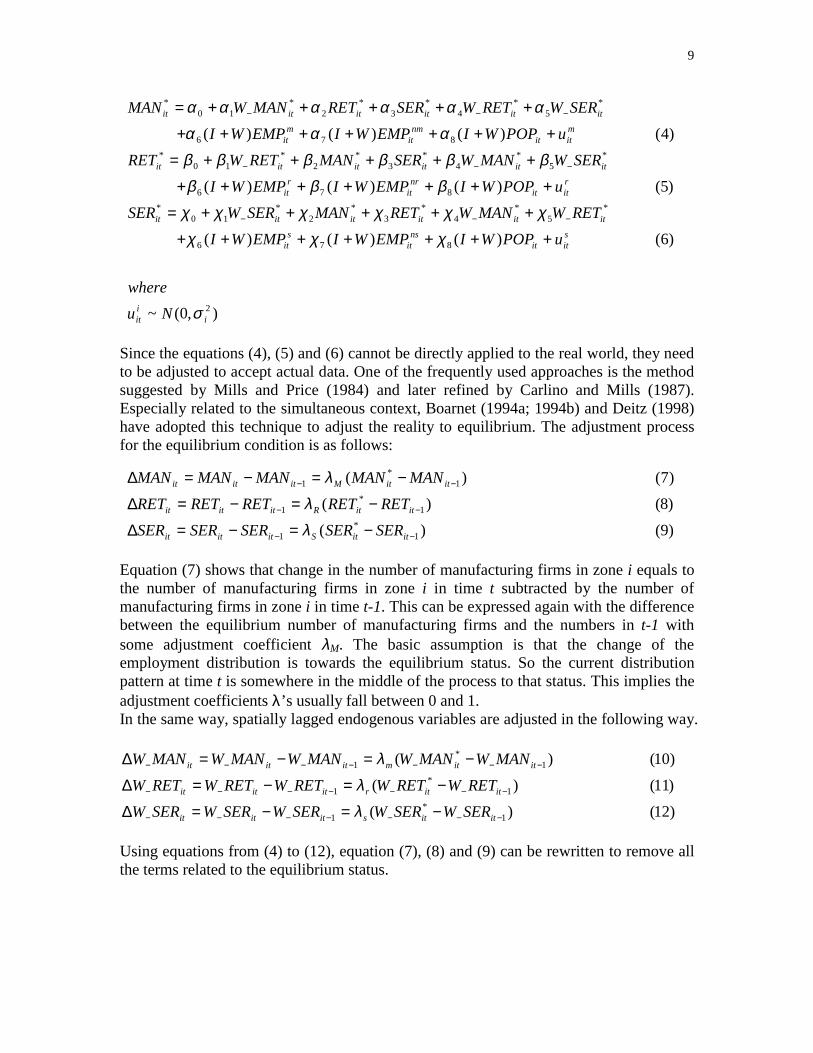
Since the equations (4), (5) and (6) cannot be directly applied to the real world, they need to be adjusted to accept actual data. One of the frequently used approaches is the method suggested by Mills and Price (1984) and later refined by Carlino and Mills (1987). Especially related to the simultaneous context, Boarnet (1994a; 1994b) and Deitz (1998) have adopted this technique to adjust the reality to equilibrium. The adjustment process for the equilibrium condition is as follows:

Equation (7) shows that change in the number of manufacturing firms in zone i equals to the number of manufacturing firms in zone i in time t subtracted by the number of manufacturing firms in zone i in time t-1. This can be expressed again with the difference between the equilibrium number of manufacturing firms and the numbers in t-1 with some adjustment coefficient λM. The basic assumption is that the change of the employment distribution is towards the equilibrium status. So the current distribution pattern at time t is somewhere in the middle of the process to that status. This implies the adjustment coefficients λ’s usually fall between 0 and 1. In the same way, spatially lagged endogenous variables are adjusted in the following way.

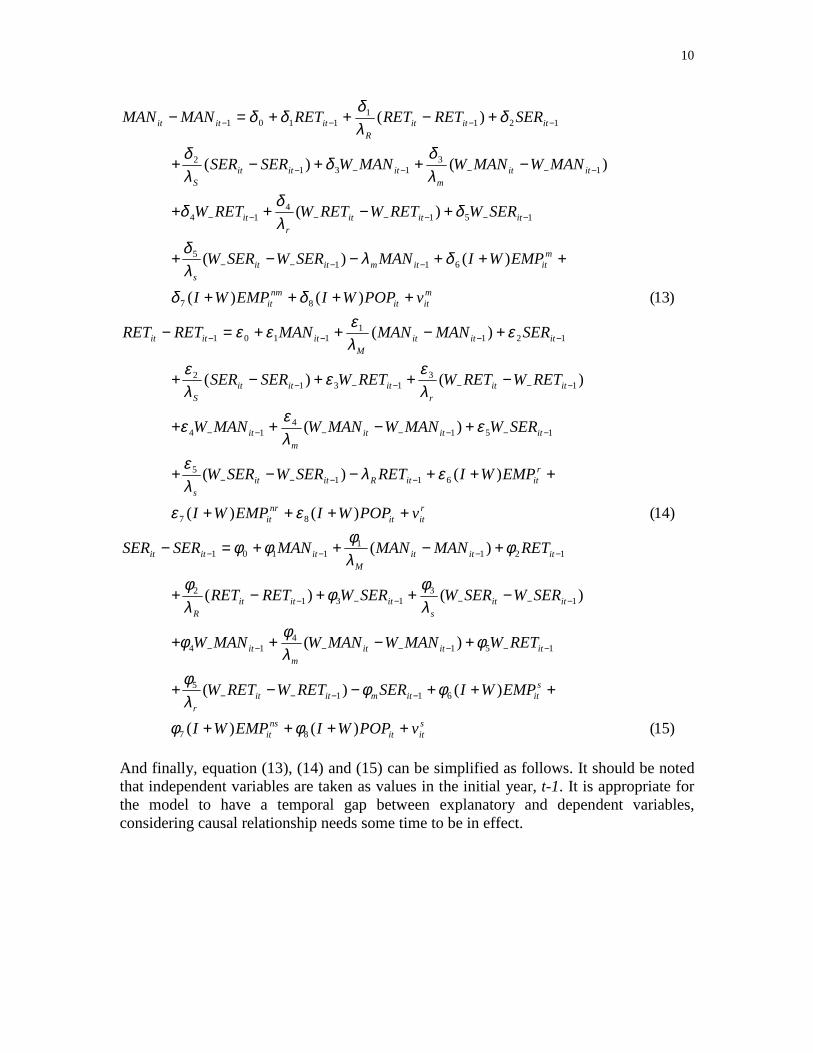
Using equations from (4) to (12), equation (7), (8) and (9) can be rewritten to remove all the terms related to the equilibrium status.

),0(~

)6()()()(

)5()()()(

)4()()()(

2

876

*5

*4

*3

*2

*10

*876

*5

*4

*3

*2

*10

*876

*5

*4

*3

*2

*10

*

iiit

sitit

nsit

sit

itititititit

ritit

nrit

rit

itititititit

mitit

nmit

mit

itititititit

Nuwhere

uPOPWIEMPWIEMPWIRETWMANWRETMANSERWSER

uPOPWIEMPWIEMPWISERWMANWSERMANRETWRET

uPOPWIEMPWIEMPWISERWRETWSERRETMANWMAN

σ

χχχχχχχχχ

βββββββββ

ααααααααα

+++++++

+++++=

+++++++

+++++=

+++++++

+++++=

−−−

−−−

−−−

)9()(

)8()(

)7()(

1*

1

1*

1

1*

1

−−

−−

−−

−=−=∆

−=−=∆

−=−=∆

ititSititit

ititRititit

ititMititit

SERSERSERSERSERRETRETRETRETRET

MANMANMANMANMAN

λλ

λ

)12()(

)11()(

)10()(

1*

1

1*

1

1*

1

−−−−−−−

−−−−−−−

−−−−−−−

−=−=∆

−=−=∆

−=−=∆

ititsititit

ititrititit

ititmititit

SERWSERWSERWSERWSERWRETWRETWRETWRETWRETW

MANWMANWMANWMANWMANW

λλ

λ

10

And finally, equation (13), (14) and (15) can be simplified as follows. It should be noted that independent variables are taken as values in the initial year, t-1. It is appropriate for the model to have a temporal gap between explanatory and dependent variables, considering causal relationship needs some time to be in effect.

)15()()(

)()(

)(

)()(

)(

)14()()(

)()(

)(

)()(

)(

)13()()(

)()(

)(

)()(

)(

87

6115

1514

14

13

1312

1211

1101

87

6115

1514

14

13

1312

1211

1101

87

6115

1514

14

13

1312

1211

1101

sitit

nsit

sititmitit

r

itititm

it

itits

itititR

itititM

ititit

ritit

nrit

rititRitit

s

itititm

it

ititr

itititS

itititM

ititit

mitit

nmit

mititmitit

s

itititr

it

ititm

itititS

itititR

ititit

vPOPWIEMPWI

EMPWISERRETWRETW

RETWMANWMANWMANW

SERWSERWSERWRETRET

RETMANMANMANSERSER

vPOPWIEMPWI

EMPWIRETSERWSERW

SERWMANWMANWMANW

RETWRETWRETWSERSER

SERMANMANMANRETRET

vPOPWIEMPWI

EMPWIMANSERWSERW

SERWRETWRETWRETW

MANWMANWMANWSERSER

SERRETRETRETMANMAN

++++

+++−−+

+−++

−++−+

+−++=−

++++

+++−−+

+−++

−++−+

+−++=−

++++

+++−−+

+−++

−++−+

+−++=−

−−−−

−−−−−−−

−−−−−−

−−−−

−−−−

−−−−−−−

−−−−−−

−−−−

−−−−

−−−−−−−

−−−−−−

−−−−

φφ

φφλφ

φλφφ

λφ

φλφ

φλφφφ

εε

ελλε

ελεε

λεε

λε

ελεεε

δδ

δλλδ

δλδδ

λδ

δλδ

δλδδδ

11

4. Estimation Methods

Traditional estimation method for simultaneous equation systems is two-stage least squares (2SLS) estimation. Rather than directly using actual endogenous variables, this estimation uses projected values of those variables in the regression. Focusing on the 1st equation of the simultaneous equation model, the estimators are obtained in the following way.

While simultaneity can be adjusted by 2SLS estimation, spatial factors remains as another factor that possibly leads to biased estimator. Rey and Boarnet (1998) have tested various, different estimators that explicitly incorporate spatiality using Monte Carlo simulation. The result showed that the Kelejian-Robinson-Prucha (KRP) estimator performed relatively well compared with other estimators. The KRP estimator, developed in a series of paper by Kelejian and Robinson (1993) and Kelejian and Prucha (1998) is based on 2SLS. However, the difference between the 2SLS and the KRP estimator is that the latter also incorporates spatially lagged independent variables in the projection matrix. As a result, the estimator takes on the following form:

)18()()()(

)()()()()(

)17()()()(

)()()()()(

)16()()()(

)()()()()(

191817

161514

3210

191817

161514

3210

191817

161514

3210

sitit

nsit

sit

ititit

iiii

ritit

nrit

rit

ititit

iiii

mitit

nmit

mit

ititit

iiii

vPOPWIEMPWIEMPWISERWIRETWIMANWIRETWIMANWISERWSER

vPOPWIEMPWIEMPWISERWIRETWIMANWISERWIMANWIRETWRET

vPOPWIEMPWIEMPWISERWIRETWIMANWI

SERWIRETWIMANWMAN

+++++++

++++++∆++∆++∆+=∆

+++++++

++++++∆++∆++∆+=∆

+++++++

++++++∆++∆++∆+=∆

−−−

−−−

−

−−−

−−−

−

−−−

−−−

−

ηηηηηη

ηηηηγγγγγγγγγγϕϕϕϕϕϕϕϕϕϕ

],,[)(

ˆˆ,ˆ

]ˆ,ˆ,ˆ,[

],,[ˆ

)19()(ˆ

3211

113322

1321

90

11

2

xxxxandxxxxppWyyWandpyypyy

yWyyxz

where

yzzzSLS

=′′=

===

=

=

′′=

−

−

ϕϕθ

θ

!

12

Since the simultaneous model in this paper implicitly includes those spatial effects in the form (I+W), it is not clear and as a result it is worthwhile to check how they are different in such a situation. The result in the following section is based on those two estimators.

5. Empirical Results: Spatial Economy in Chicago The empirical analysis was performed on 306 zip code zones in the Chicago CMSA. Variables used in the model were obtained from 1990 U.S. Population Census, 1992 U.S. Economic Census and 1995 Zip Code Business Pattern. All the variables were standardized by dividing themselves by their corresponding areal sizes. By so doing, the areal size effect could be eliminated. Two estimators described in the previous section were used to check whether the model is robust. The results from 2SLS and KRP estimation are shown in tables 1 and 2, respectively. Overall, the results from different estimation methods are not very much different from each other. They both have similar R2 values for individual sectors. Estimated coefficients are also similar especially in terms of their signs and magnitude. There are, however, several conflicting signs between two coefficients.6 But since any of them does not have significant t-value in the regression models of both estimation methods, they are not thought of as critical parts of the model.7 In the manufacturing sector, the distribution pattern of manufacturing in the previous stage ((I+W)_MAN92) plays an important role in the increase/decrease of the number of manufacturing firms. In other words, if a certain zone has more concentrated manufacturing activities in the previous stage, the zone will experience a greater number of manufacturing firms concentrating in the future. The explanation may be traced to the fact that zones with a larger number of manufacturing firms in an earlier time usually have relatively well maintained infrastructure for the manufacturing firms and well established production networks between firms. These kinds of favorable economic environments will work as attraction factors to other manufacturing firms. Note also that the spatially lagged dependent variable (W_∆MAN) has a positive relationship with the

6 Those variables are (I+W)_MEMP90, (I+W)_NMEMP90 and W_∆MAN in the manufacturing equation and (I+W)_ ∆MAN in the service equation. 7 In light of agglomeration economies, those variables would be expected to show positive signs, while two employment-related variables ((I+W)_MEMP90 and (I+W)_NMEMP90) might also have negative influences. That is, higher number of employees attracts more firms, which eventually leads to severe competition for limited production factors other than labor in a limited area.

],,,,,[)(

ˆˆ,ˆ

]ˆ,ˆ,ˆ,[

],,[ˆ

)20()(ˆ

3213211

113322

1321

90

11

WxWxWxxxxxandxxxxppWyyWandpyypyy

yWyyxz

where

yzzzKRP

=′′=

===

=

=

′′=

−

−

ϕϕθ

θ

!

13

dependent variable even though it is not significant in explaining the changing number of manufacturing firms. This implies that agglomeration process of manufacturing is self-reinforcing possibly through backward and forward linkage processes for demand and supply side of the economy respectively. 8 While retail sectors in the previous time ((I+W)_RET92) exert a negative influence on the expansion of manufacturing sectors, contemporary changes in retail firms ((I+W)_∆RET) provide a positive influence. The coefficient of the former is very small in absolute terms, so that the explanation afforded will be limited. The latter implies that manufacturing is growing in concert with retail sectors as can be confirmed again later in the retail equation. In other words, there seems to be a simultaneous interaction between the two sectors that keeps nurturing each other. The service sectors in the previous stage ((I+W)_SER92) are not significant, but the contemporary change of the same sector ((I+W)_∆SER) has a negative influence on manufacturing. Since many of the recently growing service firms in Chicago are performing higher functions such as business services, they need to be located in central places (mostly, CBD) with higher rents. Accordingly, manufacturing firms cannot compete with them for in the same zone and surrounding areas. As a result, an increase in service firms works as a repellent factor for manufacturing firms. The table also reveals that the location decision of manufacturing firms may not be affected by either the distribution of the labor force ((I+W)_MEMP90 and (I+W)_NMEMP90) or the size of the market ((I+W)_POP90).9

Table 1. Estimation results using 2SLS estimator

Variable name Manufacturing Retail Service

Constant .00556 (.447)

-.39698 (.018) *

-1.26106 (.096)

(I+W)_MAN92 .03731 (.000)**

-.07399 (.160)

.16894 (.309)

(I+W)_RET92 -.00221 (.000) **

.00990 (.001) ** N/A

(I+W)_SER92 .00044 (.724) N/A -.01040

(.086)

(I+W)_MEMP90 .00007 (.943)

(I+W)_NMEMP90 .00003 (.389)

(I+W)_REMP90 -.00096 (.137)

(I+W)_NREMP90 49.2196 (.024) *

Exogenous Variables

(I+W)_SEMP90 -.00191 (.544)

8 For more discussion on backward and forward linkages, refer to Fujita, Krugman and Venables (1999). 9 Note that market may be outside metro area of Chicago due to the hollowing-out process. For more detailed exploration of hollowing-out process in Chicago economy, refer to Hewings et al. (1998).

14

(I+W)_NSEMP90 16.4606 (.004) **

(I+W)_POP90 .08340 (.268)

.86127 (.260)

6.7446 (.000) **

(I+W)_∆MAN 1.1663 (.000) **

4.1234 (.331)

(I+W)_∆RET .82987 (.000) ** 1.64873

(.012) * (I+W)_∆SER

-.07297 (.000) **

.36937 (.000) **

W_∆MAN .46238 (.766)

W_∆RET 87.4339 (.029) *

Endogenous Variables

W_∆SER 3.29021 (.172)

Adj-R2 .5066 .4714 .8809 Note: * significant at 0.05 and ** significant at 0.01.

N/A Variables are eliminated from the list due to the multicollinearity problem. In the retail equation, a similar analogy can be applied to the relationship between manufacturing and retail sectors,10 confirming the interactions between the two sectors again from a locational perspective. Two coefficients of retail sectors ((I+W)_RET92 and W_∆RET) show positive signs, implying that self-reinforcing concentration is in progress in this sector. As a result, other things being equal, strong agglomeration will be observed in terms of the distribution in retail firms possibly due to the external economies of a region.11 An increase in the number of service firms ((I+W)_∆SER) also provides an attracting factor to retail firms, in large part because many retail functions serve people within the same geographic area. As a result, an increase in the number of service firms, such as offices, gives rise to an increase in the number of people working in the offices, the retail market is enlarged and finally a larger number of retail firms (such as restaurant or shops) move in. Even though increases in the labor force in the retail sector ((I+W)_REMP90) generate a negative influence on the growth of the retail sector in a zone, the magnitude is small, and as in the manufacturing sector, it can be ignored. The number of non-retail employees ((I+W)_NREMP90) is interpreted in two ways: (1) attraction factor for non-retail firms to be close to the labor force as the ‘jobs follow people’ hypothesis promotes, and (2) narrowly defined market composed of pure consumers that separates retail employees as suppliers, as opposed to the comprehensive market composed of total population. Since any of the sectors has a strong relation between their locations and the distribution of employees in the corresponding sectors in the table, the first interpretation may not be so plausible in this case. Rather, (I+W)_NREMP90 is viewed as the market for retail sectors along with (I+W)_POP90. 10 For example, (I+W)_MAN92 and (I+W)_∆MAN have conflicting signs and the coefficient of the former is very small compared to the latter. 11 It is not unusual in that many retail outlets concentrate in some parts of a city rather than be dispersed, which ultimately gives external economies to the firms located in such area.

15

Those two have positive relations with the growth of retail sectors, implying that the larger size of the market is in favor of concentration of retail sectors.

Table 2. Estimation results using KRP estimator

Variable name Manufacturing Retail Service

Constant .00718 (.294)

-.02136 (.165)

-.58548 (.000) **

(I+W)_MAN92 .01974 (.000) **

-.05285 (.000) **

.30878 (.000) **

(I+W)_RET92 -.00192 (.000) **

.00456 (.000) **

-.00795 (.641)

(I+W)_SER92 .00105 (.370) N/A -.00491

(.048) *

(I+W)_MEMP90 -.00038 (.690)

(I+W)_NMEMP90 -.00001 (.653)

(I+W)_REMP90 -.00076 (.010) **

(I+W)_NREMP90 13.0333 (.000) **

(I+W)_SEMP90 -.00069 (.950)

(I+W)_NSEMP90 15.4653 (.002) **

Exogenous Variables

(I+W)_POP90 .04370 (.512)

.29782 (.066)

4.87691 (.000) **

(I+W)_∆MAN 1.10479 (.000) **

-1.37942 (.328)

(I+W)_∆RET .72747 (.000) ** 2.41008

(.000) ** (I+W)_∆SER

-.04673 (.000) **

.10098 (.000) **

W_∆MAN -1.15569 (.766)

W_∆RET 1.20468 (.359)

Endogenous Variables

W_∆SER 1.18115 (.000) **

Adj-R2 .5571 .3114 .8960 Note: * significant at 0.05 and ** significant at 0.01.

N/A Variables are eliminated from the list due to the multicollinearity problem. In the service sector, the distribution of manufacturing firms in the previous stage ((I+W)_MAN92) may affect the change in the number of service firms ((I+W)_∆MAN) in

16

a positive way. On the other hand, changes in the number of manufacturing firms are not so relevant to those of service firms. One explanation is that service firms prefer to choose locations in which large pool of manufacturing firms are already established than choosing locations in growing manufacturing regions. This will be the case for producer services, as the number of manufacturing firms will decide the size of the market for these service firms. In this sense, a mature market should be a more stable option for the firms than a growing regional market. An increase in retail firms ((I+W)_∆RET) has a positive influence on increase in the service firms. As mentioned in the retail equation, this is a further example of the synergetic effect between two sectors. For example, some retail firms gather to serve people in service firms and then in turn another types of service firm form to serve those retail firms (for such matters as tax-related, accounting or consulting). Two coefficients related to the distribution of service sectors ((I+W)_SER92 and W_∆SER) reveal that change in the number of service firms in a region is negatively related to the initial distribution of service firms and positively related to the change in the number of firms around the region (W_∆SER). If there are a lot of service firms in a region, it means there should be severe competition among service firms as well as a certain advantages such as external economies. If the service market is almost saturated, then the disadvantage from the former may be larger than the advantage from the latter. If this is the case, a negative relationship will be observed between the two variables. On the other hand, an increasing number of service firms in a region reflects that the market is not yet fully covered, leading to more entry of service firms in the region until the market becomes full of suppliers. Service sectors are also insensitive to the distribution of the labor forces ((I+W)_SEMP90) as the two previous sectors are. Again, the same explanation can be applied to non-service sector labor forces ((I+W)_NSEMP90) and population ((I+W)_POP90) as in retail sectors. The larger market leads to the concentration of service firms. Finally, in terms of the explanatory power, the equation for services has the highest R2 value, followed by manufacturing and retail. The relatively lower levels of R2 for the retail sector seem to be ascribed to the spatial distribution characteristics of the sector. That is, retail firms are distributed over the space more evenly to have an easy access to and from customers (mostly people rather than firms) following the general rule of the spatial market. As a result, it is hard to identify a particular spatial pattern for the retail sector and to explain the pattern with other types of spatial distribution patterns (for example, of independent variables). Manufacturing and service sectors are thought of as having more localized characteristics in terms of the spatial distribution, which are relatively well matched with the distribution patterns of other explanatory variables.

6. Conclusion This paper attempted to adapt the spatial econometric version of the simultaneous equation system to examine the spatial evidence of agglomeration economies in Chicago in the 1990s. Three economic sectors (manufacturing, retail and service) were considered and as a result three equations were obtained using 2SLS and KRP estimation methods. While detailed interpretations were provided in the previous section, there are several interesting results to be noted.

17

Figure 1. Endogenous relationship among three sectors First, in terms of the backward- and forward-linkage effects between industries, there was some evidence that external economies and, as a result, possible agglomeration economies were observed between manufacturing and retail sectors and between retail and service sectors. However, there was no such effect between manufacturing and service sectors. Rather, the relationship showed more dominant repellent forces between two sectors, especially from service to manufacturing. There was also a mild tendency that retail and service sectors are self-reinforcing in that they attract more and more activities of a similar type in the same zone or surrounding area. Figure 1 summarizes the endogenous relationships among the three economic sectors. Secondly, if attention is directed to the previous economic settings or environment, the inter-industry relation might be a little different from the one when investigating endogenous relations. Either manufacturing or retail sector could be considered an attractive incubator to the other when firms make decisions on location and/or consider relocation. While the size of individual sector in a zone (number of firms in a sector) is not an incentive for firms in other sector to move in, the growth of the sector in the zone (change in number of firms in a sector) is revealed as an attraction factor between manufacturing and retail sectors. From the view of the retail sector, fully-grown manufacturing areas may already have enough number of retail facilities to serve them, whereas growing manufacturing markets provide more opportunities. From the view of the manufacturing sector, a fully-grown retail area may not be considered a proper location for them in large part due to relatively high rent, lack of available vacant space and so forth. The manufacturing sector, however, is functioning as an incubator for the service sector, especially for producer services.12 Finally, a higher level of economic activities in the same sector in the previous time period works as an attraction factor (incubator rather than higher competitive market) for manufacturing and retail sectors while a repellent (higher competitive market rather than incubator) for the service sector. Figure 2 shows the relationships among sectors.

12 In a sense, positivity in endogenous relationship between manufacturing and retail and positivity in exogenous relationship between manufacturing and service may be related to the time lag required for the firms in each sector to react to the changing environment. That is, retail firms are seen to respond faster to the change in the economic environment than service firms.

Manufacturing

Retail Service

+ +

+

+ + +

_

18

Figure 2. Exogenous relationship among three sectors Third, the traditional hypothesis, “jobs follow people,” was not proven to be true in an intra-urban context in Chicago. None of the three sectors showed a significant influence from this variable. For example, the distance between home and work, or closeness to the labor force may not be such important considerations within a city, while obviously important in intercity or interregional contexts. Finally, closeness to market (represented by population and number of employees in other sectors) did not provide significant explanatory power overall even though there are a few significant variables. However, those variables deal only with the distribution of people through their residences. In other words, if the distribution of people in terms of workplace (i.e. number of employees in a zone) is considered, that will be another comparable market for firms.13 And the resulting explanation of the variable will be more improved. Possible extensions to this analysis would be to incorporate general microeconomic relationships of consumers and producers in the spatial market. Related to this issue, it will be challenging to link zone-based model like this with firm-based model of most microeconomic models that include the production function of individual firms. Finally, an obvious extension would be further more disaggregation in the level of interaction between sectors. For example, the relationship between a specific type of manufacturing and producer service will be clearer in terms of their synergetic effects on the location/distribution pattern of each sector.

References

Abdel-Rahman, H.M., (1990) “Agglomeration economies, types, and sizes of cities,” Journal of Urban Economics 27, 25-45.

13 For example, people may want to go shopping during the lunch hour or after the work. They may also want to do some personal businesses related to personal service firms during those time periods of a day. In this situation, they may prefer choosing closer retail and service firms from their workplaces. In the viewpoint of retail and service firms (suppliers), they may be considered another equivalent potential market.

Manufacturing

Retail Service

_

_

+ _

+

+

19

Alonso, W., (1964) Location and Land Use: Towards a General Theory of Land Rent, Harvard University Press, Cambridge, MA.

Anselin, L. and A.K. Bera, (1998) “Spatial dependence in linear regression models with an introduction to spatial econometrics,” in Handbook of Applied Economic Statistics. Edited by A. Ullah and D.E.A. Giles, Marcel Dekker, New York, NY. 237-89.

Bergsman, J., P. Greenston and R. Healy, (1975) “A classification of economic activities based on location patterns,” Journal of Urban Economics 2, 1-28.

Boarnet, M.G., (1994a) “An empirical model of intrametropolitan population and employment growth,” Papers in Regional Science 73, 135-52.

Boarnet, M.G., (1994b) “The monocentric model and employment location,” Journal of Urban Economics 36, 79-97.

Calem, P.S. and G.A. Carlino, (1991) “Urban agglomeration economies in the presence of technical change,” Journal of Urban Economics 29, 82-95.

Carlino, G.A. and E.S. Mills, (1987) “The determinants of county growth,” Journal of Regional Science 27, 39-54.

Cooke, T.W., (1978) “Causality reconsidered: A note,” Journal of Urban Economics 5, 538-42.

Cooke, T.W., (1983) “Testing a model of intraurban firm relocation,” Journal of Urban Economics 13, 257-82.

DeCoster, G.P. and W.C. Strange, (1993) “Spurious agglomeration,” Journal of Urban Economics 33, 273-304.

Deitz, R., (1998) “A joint model of residential and employment location in urban areas,” Journal of Urban Economics 44, 197-215.

Dekle, R. and J. Eaton, (1999) “Agglomeration and land rents: Evidence from the prefectures,” Journal of Urban Economics 46, 200-14.

Fogarty, M.S. and G.A. Garofalo, (1988) “Urban spatial structure and productivity growth in the manufacturing sector of cities,” Journal of Urban Economics 23, 60-70.

Fujita, M. and J.-F., Thisse, (1996) “Economics of agglomeration,” Journal of the Japanese and International Economics 10, 339-78.

Fujita, M., P. Krugman and A.J. Venables, (1999) The Spatial Economy, The MIT Press, Cambridge, MA.

Goldstein, G.S. and T.J. Gronberg, (1984) “Economies of scope and economies of agglomeration,” Journal of Urban Economics 16, 91-104.

20

Greenwood, M.J., (1980) “Metropolitan growth and the intrametropolitan location of employment, housing, and labor force,” The Review of Economics and Statistics 62, 491-501.

Greenwood, M.J. and R. Stock, (1990) “Patterns of change in the intrametropolitan location of population, jobs, and housing: 1950 to 1980,” Journal of Urban Economics 28, 243-76.

Grubb, W.N., (1982) “The flight to the suburbs of population and employment, 1960- 1970,” Journal of Urban Economics 11, 348-67.

Hansen, E.R., (1990) “Agglomeration economies and industrial decentralization: The wage-productivity trades-offs,” Journal of Urban Economics 28, 140-59.

Hanson, G.H., (1996) “Agglomeration, dispersion, and the pioneer firm,” Journal of Urban Economics 39, 255-81.

Helsley, R.W. and W.C. Strange, (1991) “Agglomeration economies and urban capital markets,” Journal of Urban Economics 29, 96-112.

Hewings, G.J.D., M. Sonis, J. Guo, P.R. Israilevich and G.R. Schindler, (1998) “The hollowing-out process in the Chicago economy, 1975-2011,” Geographical Analysis 30, 217-33.

Kelejian, H.H. and D.P. Robinson, (1993) “A suggested method of estimation for spatial interdependent models with autocorrelated errors, and an application to a county expenditure model,” Papers in Regional Science 72, 297-312.

Kelejian, H.H. and I.R. Prucha, (1998) “A generalized spatial two-stage least squares procedure for estimating a spatial autoregressive model with autoregressive disturbances,” Journal of Real Estate Finance and Economics 17, 99-121.

Lee, K.S., (1981) “Intra-urban location of manufacturing employment in Colombia,” Journal of Urban Economics 9, 222-241.

Maurel, F. and B. Sedillot, (1999) “A measure of the geographic concentration in french manufacturing industries,” Regional Science and Urban Economics 29, 575-604.

McMillen, D.P. and J.F. McDonald, (1998) “Suburban subcenters and employment density in metropolitan Chicago,” Journal of Urban Economics 43, 157-80.

Mills, E.S. and R. Price, (1984) “Metropolitan suburbanization and central city problems,” Journal of Urban Economics 15, 1-17.

Mitra, A., (1999) “Agglomeration economies as manifested in technical efficiency at the firm level,” Journal of Urban Economics 45, 490-500.

Moomaw, R.L., (1985) “Firm location and city size: Reduced productivity advantages as a factor in the decline of manufacturing in urban areas,” Journal of Urban Economics 17, 73-89.

21

Moses L.N. and H.F. Williamson, Jr., (1972) “The location of economic activity in cities,” in Readings in Urban Economics. Edited by M. Edel and J. Rothenberg, The Macmillan Company, New York, NY. 124-34.

Mun, S. and B.G. Hutchinson, (1995) “Empirical analysis of office rent and agglomeration economies: A case study of Toronto,” Journal of Regional Science 35, 437-55.

Nakamura, R., (1985) “Agglomeration economies in urban manufacturing industries: A case of Japanese cities,” Journal of Urban Economics 17, 108-24.

Palumbo, G. and P. Hutton, (1987) “On the causality of intraurban location,” Journal of Urban Economics 22, 1-13.

Pascal, A.H. and J.J. McCall, (1980) “Agglomeration economies, search costs, and industrial location,” Journal of Urban Economics 8, 383-8.

Rey, S.J. and M.G. Boarnet, (1998) “A taxonomy of spatial econometric models for simultaneous equations systems,” Paper presented in the 45th Annual North American Meetings of the Regional Science Association International, Santa Fe, NM.

Siegel, J., (1975) “Intrametropolitan migration: A simultaneous model of employment and residential location of white and black households,” Journal of Urban Economics 2, 29-47.

Simpson, W., (1980) “A simultaneous model of workplace and residential location incorporating job search,” Journal of Urban Economics 8, 330-49.

Smith, Jr., D.F. and R. Florida, (1994) “Agglomeration and industrial location: An econometric analysis of Japanese-affiliated manufacturing establishments in automotive-related industries,” Journal of Urban Economics 36, 23-41.

Steinnes, D.N., (1977) “Causality and intraurban location,” Journal of Urban Economics 4, 69-79.

Thurston, L. and A.M.J. Yezer, (1994) “Causality in the suburbanization of population and employment,” Journal of Urban Economics 35, 105-18.

Van Ommeren, J., P. Rietveld and P. Nijkamp, (1999) “Job moving, residential moving, and commuting: A search perspective,” Journal of Urban Economics 46, 230-53.