the regional economics applications laboratory (real) … · · 2008-09-16focusing on the...

The Regional Economics Applications Laboratory (REAL) is a unit in the University of Illinois focusing on the development and use of analytical models for urban and region economic development. The purpose of the Discussion Papers is to circulate intermediate and final results of this research among readers within and outside REAL. The opinions and conclusions expressed in the papers are those of the authors and do not necessarily represent those of the University of Illinois. All requests and comments should be directed to Geoffrey J. D. Hewings, Director, Regional Economics Applications Laboratory, 607 South Matthews, Urbana, IL, 61801-3671, phone (217) 333-4740, FAX (217) 244-9339. Web page: www.real.uiuc.edu/.

ECONOMIC GEOGRAPHY AND SPATIAL WAGE STRUCTURE IN SPAIN

Jesús López-Rodríguez, Miguel A. Márquez

and Andres Faiña

REAL 08-T-4 September 2008

http://www.real.uiuc.edu/

Economic Geography and Spatial Wage Structure in Spain Jesús López-Rodríguez Harvard University (USA) and University of A Coruña (Spain) Miguel A. Márquez

University of Extremadura (Spain) and Regional Economics Applications Laboratory, University of Illinois at Urbana-Champaign (USA) Andres Faiña University of A Coruña (Spain) Abstract: In this paper, the nominal wage equation of a Core-Periphery model of New Economic Geography is derived. In order to show empirical evidence of the resulting hypothesis, the nominal wage equation is estimated for the Spanish provinces in the year 2003. Our results illustrate that the market access variable is statistically significant and quantitatively important in the explanation of the spatial wage structure observed in Spain. Moreover, we show that there are at least three channels through which market access might be affecting Spanish wages: human capital, productive capital and the size of R&D activities. Key Words: New Economic Geography, Spatial Wage Structure, Market Access, Spanish Provinces JEL Classification: R11, R12, R13, R14, F12, F23

1. Introduction Economic activities tend to cluster at many geographical levels (Florence (1948), Hoover (1948),

Fuchs (1962), Enright (1990), Ellison and Glaeser (1996), Dumais et al. (1997), Porter (1998,

2000). At a world wide level, there is the North-South dualism where NAFTA (North American

Free Trade Agreement- US-Canada-Mexico) the EU-15 countries and East Asia account for 83%

of the world’s GDP in the year 2000. Furthermore, Hall and Jones (1999) observe that high-

income nations are clustered in small cores in the Northern hemisphere and that productivity per

capita steadily declines with increasing distance from the core regions (New York, Brussels and

Tokyo). Moving to a smaller geographic scale, the so called “blue banana” in the European

Union1 is well known case: a large agglomeration area that takes in Greater Manchester, London,

Paris, Northern Italy and the Ruhr Valley. This area represents roughly 20% of the former EU15,

1For a comprehensive analysis of the spatial structure of Europe see Faíña et al. (2001), Faíña and Lopez-Rodriguez (2006b). A similar case is the “US manufacturing belt” in the East coast of the United States.

R E A L Economic Geography and Spatial Wage Structure in Spain 3

but contains 40% of its GDP and 50% of its population (see Lopez-Rodriguez et al. 2007). At

the country level, the case of the Île-de-France (the metropolitan area of Paris) which accounts

for 2.2% of the area of the country and 18.9% of its population and produces 30% of its GDP is a

clear example of the clustering of economic activities in a space.2 In the case of Spain, and in

terms of the New Economic Geography literature, a “core-periphery” structure can also be

defined. There, the “core” (the triangle area comprising the axis Basque Country-Gerona,

Gerona-Valencia and Valencia-Basque Country plus the capital, Madrid) represents a quarter of

the total Spanish Peninsular area but concentrates almost 50% of its population and 60% of its

GDP; whereas the rest of the country could be characterized in a New Economic Geography

fashion as the Spanish “periphery” with less economic activity and a much lower level of per

capita income (see Faiña and Lopez-Rodriguez 2006a). Thus, a number of papers have recently

presented evidence about the tendency for Spanish economic activity to be geographically

concentrated, where core regions are leaving behind the group of peripheral regions (Márquez

and Hewings, 2003; Márquez et al 2003; and Márquez et al 2006).

<<Insert table 1 here>> <<insert figure 1 here>>

Figure 1 shows the distribution of per capita GDP in Euros in the 47 peninsular Spanish

provinces for the years 1995 and 2004 by quantiles. From this graph and from computations in

table 1, it can be seen that disparities in terms of per capita GDP among the Spanish provinces

are still quite high and there has been little tendency for them to change.

Looking at the ratio between the capital of Spain (Madrid) and the average per capita GDP, the

figures for the year 2004 show that the income in Madrid is almost 40% higher than in the

average Spanish province. A similar ratio can also be found when the so-called Spanish “core”

is compared with the Spanish “periphery.” Comparing these computed ratios for the year 2004

with the same computations for the year 1995 (see also figure 1), it is possible to observe that per

capita GDP disparities either between Madrid and the average provincial per capita GDP of the

“core” and the “periphery” have not changed. On the contrary, there was a slight increase. In

addition, these disparities show a well defined income gradient, in the sense that provincial per

capita GDP is a decreasing function of the distance from Zaragoza (a proxy for the geographical

2Sao Paulo with 18 million population but 15% of Brazilian GDP is another example of a high concentration of economic activities in a space.


center of the so-called Spanish “core”). Figure 2 illustrates the relationship between provincial

per capita GDP and distance from Zaragoza for the year 2004.

<<insert figures 2, 3 here>>

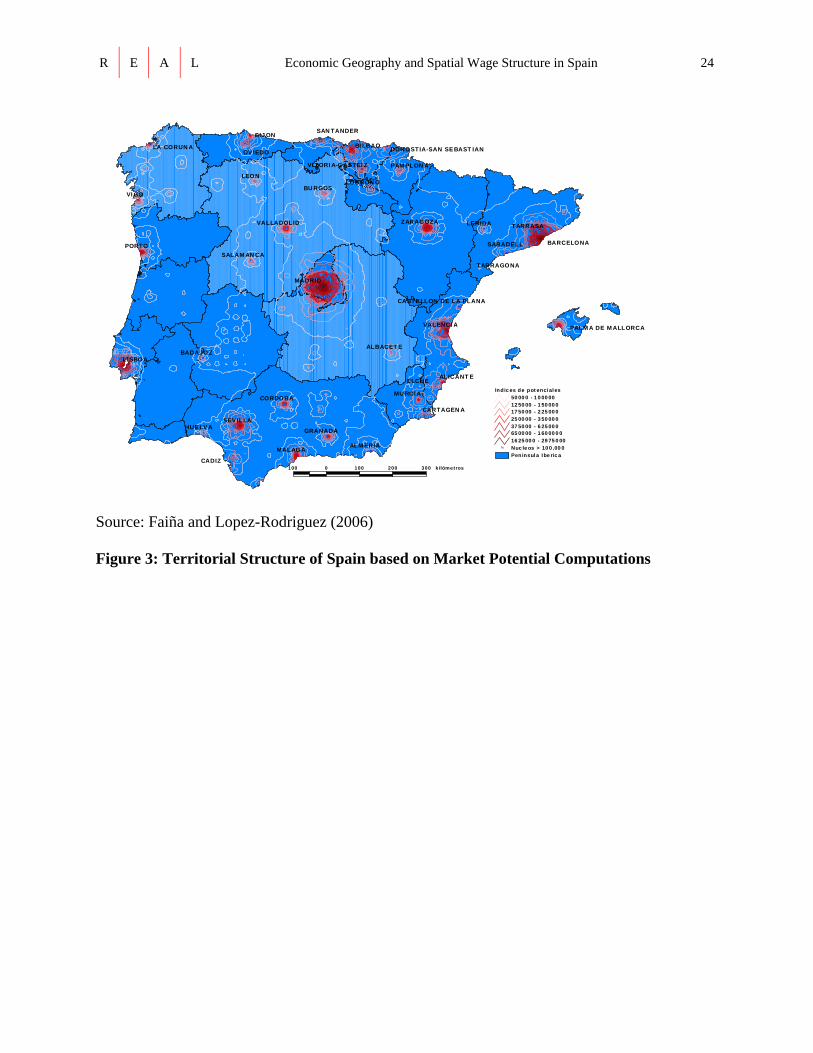
Another way of looking at the core-periphery structure is by computing indexes of market

potential. Figure 3 represents the territorial structure of Spain based on market potential

computations. In this figure, it can also be appreciated that the highest values of market potential

are found in the Mediterranean façade along the triangle defined by the Basque Country-Gerona-

Valencia plus the capital Madrid, whereas the lowest market potential values are observed on the

Atlantic façade.

There are many theories that explain the lack of convergence among countries or regions. From

the point of view of growth theories, Barro and Sala-i-Martin, (1991, 1995) show that differences

in saving rates, investment rates, human capital levels, sluggish technological diffusion, etc. may

prevent income levels from moving closer together. Traditional theories of economic

development emphasize the role of first nature geography (access to waterways, ports, airports,

hydrocarbons, climate conditions) in determining income levels (see Hall and Jones, 1999). In

the early 1990s, a new branch of research within the spatial economics began with the pioneering

works of Krugman (1991a, b). The so-called New Economic Geography added new insights and

provided micro foundations to the explanation of why economic activities are clustered in space.

This new line of research which the building blocks are increasing returns to scale at the firm

level, transportation costs and imperfect competition emphasize the role of the so-called second

nature geography (distance to consumer markets and distance to input suppliers) as opposed to

first nature geography as a way of explaining differences in income levels among regions or

countries. Krugman’s (1991a, b) contributions have generated a plethora of theoretical

contributions. However, empirical research is still lagging behind. The first empirical attempt to

validate the forces at work in the New Economy Geography models at the country level was

made by Hanson (1998, 2005) for the United States. Since Hanson’s contributions, many other

scholars have tried to test the theoretical predictions of New Economic Geography models for

different geographical settings. For instance, Redding and Venables (2004) tested a NEG model

for a sample of world countries, Breinlich (2006), Head and Mayer (2006) and Lopez-Rodriguez

and Faiña (2007) tested it for different samples of European Union regions. Brackman et al.


(2004), Combes and Lafourcale (2004), Roos (2001) and Pires (2006)3 center their analysis on

single countries.

The main goal of this paper is to contrast the theoretical predictions of core-periphery New

Economic Geography models about the important role played by second nature geography in

explaining per capita GDP disparities. The empirical evidence is presented by estimating a

derived nominal wage equation for the set of the 47 Spanish peninsular provinces in the year

2003. Our results prove to be robust with the established hypothesis, contributing to the

empirical literature on New Economic Geography. Moreover, the obtained results show that

there are at least three channels through which market access might be affecting Spanish wages:

human capital levels, productive capital and the size of R&D activities.

The remaining part of the paper is structured as follows. Section 2 presents the theoretical

framework. Section 3 deals with the econometric specifications, data base and variables used in

the empirical analysis. In addition, the results and discussions of the econometric estimations are

presented. Finally, section 5 offers the main conclusions.

2. Theoretical Background: New Economic Geography and Market Access

The theoretical framework is a reduced version of a standard New Economic Geography model

(multi-regional version of Krugman, 1991b) that incorporates the key elements to derive the so-

called wage equation and market access. The wage equation will form the basis of the empirical

estimations.

Consider a regional setting composed of R locations ( =1, 2……….R), focusing on the

analysis of the manufacturing sector. In this sector, firms produce a great number of varieties of

a homogenous differentiated good (D) under increasing returns to scale and monopolistic

competition. Firms face transport costs in an iceberg

j

4 form in order to receive one unit of the

differentiated good at location j from location i , units must be shipped from i, so

measures the fraction of good that is melted in transit from i to . The manufacturing sector can

1, >jiT 1, −jiT

j

3 A recent and extensive survey of the empirical literature on New Economic Geography models can be seen in López-Rodríguez and Faiña (2008). Other surveys are those of Overman et al. (2003), Combes and Overman (2004) and Head and Mayer (2004). 4 See McCann (2005) for a discussion on some problems with the iceberg assumption.


produce the differentiated good in different locations. On the demand side, the final demand in

location j can be obtained via utility maximization of the corresponding CES utility function:

, ( )

maxi j

jm z

D (1)

where represents the consumption of the differentiated good in location . D is an aggregate

of industrial varieties defined by a CES function a la Dixit and Stiglitz (1977):

jD j

11

,10

( )in

Rj i ji

D m z dz

σσ

σσ

−−

=

⎡ ⎤= ⎢ ⎥⎢ ⎥⎣ ⎦∑ ∫ (2)

where is the consumption of the each available variety in location that is produced in

location and is the number of varieties produced in location i .

)(, zm ji z j

i in σ represents the elasticity

of substitution among the varieties of the differentiated good where 1>σ . Products are

homogeneous if σ tends to infinity and varieties are very differentiated if σ is close to one.

Consumers maximize their utility (function 1) bearing in mind the following budget constraint:

1

RD

i ij ij ji

n x p Y=

=∑ (3)

The consumer’s problem solution gives the final demand in location j for each variety produce in

location i.

11

1

RDij ij n nj jn

x p n pσ σ−

− −=

⎡ ⎤= ⎣ ⎦∑ Y (4)

where ( is the price of varieties produced in location i and sold in and

represents the total income in location .

ijp ),ijiij Tpp = j jY

j

If we define a price index for the differentiated goods5 1

111

Rj n njn

P n p σσ −−=

⎡ ⎤= ⎣ ⎦∑ and rewrite the

consumption expenditure as , final demand in location can be written as

. However, in order for units of consumption to arrive at location ,

jj YE = j

jjijconsDij EPpx 1−−= σσ consD

ijx j

5 This Industrial Price Index in location j measures the minimum costs of purchasing a unit of the composed index of manufacturing goods D so it can be interpreted as an expenditure function.


1

consDijji xT , must be shipped. So the effective demand a firm in location i faces from a consumer in

location j is given by:

1 1Dij ij ij j j i ij j jx T p P E p T P Eσ σ σ σ σ− − − − −= = (5)

On the supply side a typical firm in location i maximizes the following profit function:

1 ,

( )DR

ij ij D Di i

j i j

p xw F cx

T=

∏ = − +∑ i (6)

Technology in the increasing returns to scale manufacturing sector is given by the usual linear

cost function: where represents the industrial workers used for the

production of a variety in location i and sold in location , represents a fixed cost of

production, is the variable unit cost and is the amount of the differentiated good demanded

in location and produced in location i (

,DijDij cxFl += ,Dijl

j ,F

,c Dijx

j ∑≡j

Dij

Di xx represents the total amount of output

produced by the firm in location i and sold in the different locations) and is the nominal

wage paid to the manufacturing workers in location i . The assumptions of increasing returns to

scale, preference for variety by consumers, and the existence of an infinite number of varieties of

the differentiated good means that each variety is going to be produced by a single specialized

firm in only one location. In this way, the number of the manufacturing firms is exactly the same

as the number of available varieties. Each firm maximizes its profit behaving as a monopoly of

its own variety of the differentiated good. First order conditions for profit maximization yield

the standard result that prices are set as a constant mark-up over marginal costs.

j Diw

1D

i ip w cσσ

=−

(7)

where 1−σ

σ represents the Marshall-Lerner price-cost mark-up. The higher this ratio, the

higher the degree of monopoly power by a firm. As a result, Krugman (1991b) interprets σ as

an inverse measure of scale economies since it can be thought as a direct measure of price

distortion and as an indirect measure of market distortion due to monopolistic power. Given that


1−σσ is greater than one, Krugman (1991b) interprets this result as a way of justifying the

existence of increasing returns to scale. If this pricing rule is substituted into the profit function,

the following expression for the equilibrium profit function can be obtained:

( ) 1

DD i

i icxwσ⎡ ⎤

∏ = −⎢ −⎣ ⎦F ⎥ (8)

Free of entry assures that in the long run firms break even. So, the incentives for a firm to

relocate in a different location have vanished. This implies that the equilibrium output is the

following:

( 1Di

Fx xcσ −

= =) (9)

The price that is needed to sell this amount of output is ∑=

−−−=

R

jjijji TPE

xP

1

1,

11 σσσ . This expression

is combined with the fact that in equilibrium prices are a constant mark-up over marginal costs,

the following zero-profit condition can be obtained:

1

1 1,

1

1 1 RDi j j

j

w E Pc x i jT

σσ σσ

σ− −

=

⎡ ⎤−⎛ ⎞= ⎢⎜ ⎟⎝ ⎠ ⎣ ⎦

∑ ⎥ (10)

This equation is the so-called nominal wage equation in the literature of New Economic

Geography, and constitutes the key relationship that is going to be empirically tested. Equation

(10) shows that the nominal wage level at location i depends on a weighted sum of the

purchasing power of the surrounding locations where the weighted scheme is a distance function

that decreases as the distance between i and j increases. In the New Economic Geography

Literature, the right hand side of the expression (10) has different names; the most common are

market access (see Redding and Venables, 2001, 2004) and real market potential (see Head and

Mayer, 2004). Here, this expression will be referred as market access, and it will be denoted by

MA. The meaning of this equation is that those firms in locations that have a good access to big

markets (high market access) will tend to remunerate their local factors of production (workers)

with better salaries due to their savings in transportation costs.


If we normalize output production choosing our units in such a way that σ

σ )1( −=c , and we set

the fixed input requirement as σ1

=F , and define market access in location i as

, we can rewrite the nominal wage equation as: ∑=

−−=R

jjijji TGEMA

1

1,

1 σσ

[ ]1Di iw MA σ= (11)

This simplification in the nominal wage equation is very similar to the Harris (1954) market

potential function in the sense that the economic activity is higher in those regions that are closer

to big markets. So, New Economic Geography gives the micro-foundations for the ad-hoc

formulation of the Harris (1954) market potential formulation.

3. Data and results

In this section, in order to show empirical evidence of the resulting hypothesis raised in section 2,

the nominal wage equation for the Spanish provinces in the year 2003 is estimated. The research

strategy will be the following. As a starting point for the regional investigation, a basic

relationship is estimated. As this basic regression could be merely informative, a conditioning

scheme should be undertaken, the unconditional baseline regression is transformed to a

conditional one, informing about the relevance of the market access variable under the inclusion

of control variables that might be affecting Spanish wages.

3.1. Econometric specification: baseline regression

Taking logs in the expression (11), the estimation of the nominal wage equation is based on the

estimation of the following expression:

[ ]1log( ) logi iw M iAθ σ η−= + + (12)

where iη represents the error term and the other variables were defined in the previous section.

This equation relates nominal wages in location i with GDP in the surrounding locations

weighted by distance and prices. In accordance with the theoretical predictions of the model, the

higher the prices and GDP in the surrounding locations and the shorter the distance between the


different locations, the higher will be the local wage. This specification captures the notion of a

spatial wage structure and allows testing for a direct relationship between nominal wages in a

particular location and its market access. This also constitutes an important condition to reveal

agglomeration dynamics.

With respect to the data for the empirical illustration, we proxy the “wage” variable of the model

by the provincial per capita GDP expressed in Euros for the corresponding year of analysis, 2003.

With respect to the “market access” variable it is computed as a weighted sum of the GDP of the

surrounding provinces, where the weighted scheme is the distance measured in km between the

capital cities of each province. The internal distance for each province is computed as

proportional to the square root of the provinces’ area. The expression used to compute it is

πArea66.0 , where “Area” represents the size of the province in km2. This expression

generates the average distance between two points in a circular location (see Head and Mayer,

2000, Nitsch 2000 and Crozet 2004 for a discussion of this internal distance). Data on per capita

GDP and GDP for the Spanish peninsular provinces in 2003 is taken from the Spanish National

Statistical Institute (INE).6

<<insert figure 4 here>>

<<insert table 2 here>>

Presenting an exploratory data analysis, figure 4 provides a clearer view of the relationship

between provincial per capita GDP and Market Access in year 2003 by means a simple graph.

From figure 4, it seems that there is a positive relationship between the provincial per capita

GDP for year 2003 and the provincial market access. Table 2 summarizes the results of the

estimation of equation (12) for the sample of 47 Spanish provinces for the year 2003. Ordinary

Least Squares (OLS) are used in this baseline estimation (Column 1 of table 2).

From table 2, itg can be seen that there is a significant relationship between both variables. On

average, if market access increases by 1%, per capita GDP will increase by 1.26%. As a

consequence, market access would be a relevant variable in explaining the wage structure in this

Spanish system. Nevertheless, a problem we face with our baseline regression is that the

6 It is necessary to emphasize that the availability of the instrumental variables that are used in the estimation is limited to year 2003. This is the reason why year 2003 is taken as the year of analysis.


independent variable, market access, is endogenous and simultaneously determined with GDP.

This could lead to the well-known simultaneity bias in the regressions violating the necessary

conditions to obtain estimates with good properties. The standard approach to overcome the

consequences of simultaneity (biasness, inefficiency and inconsistency on OLS-estimators) is the

instrumental variables (IV) estimation. IV estimation is based on the existence of a set of

instruments that are strongly correlated to the original endogenous variables but asymptotically

uncorrelated with the error term. Once these instruments are identified, they are used to

construct a proxy for the explanatory endogenous variables which consists of their predicted

values in a regression on both the instruments and the exogenous variables. However, it is

difficult to find such instruments because most socioeconomic variables are endogenous as well.

In this work, accessibility variables have been suggest as instruments, since they are highly

correlated with the market access variable, but also noncontemporareously correlated with the

errors. Consequently, three variables are proposed as instruments. A gravity indicator of

efficiency and a location indicator, which are taken from Monzón et al. (2005)7, and a third one,

the mean time of access to a commercial airport, which is based on our own elaboration. The

gravity indicator of efficiency is an adimensional variable, and shows the role played by

infrastructures in the territorial distribution of the levels of accessibilities. It is an indicator of

relative accessibility, showing the quality of the infrastructures in the relationships between

nodes within a territory. When the value of this indicator decreases, accessibility increases. The

other accessibility indicator, location indicator, is measured in minutes, and it shows how

infrastructures enables access to the places where population is concentrated. If the value of the

location indicator decreases, accessibility increases. Both, the gravity indicator of efficiency and

the location indicator are available at the provincial level. Finally, market access is instrumented

with the variable mean time of access to a commercial airport. Data on this instrument are

available only at the regional level. Thus it was assumed that mean time of access to a

commercial airport is identical in all provinces within the same region.

IV estimation (see column 2 of table 2) again finds a positive and highly statistically significant

effects of market access, although there is a strong correction of the coefficient, changing from

1.26 to 0.16. Now, it is necessary to take into account other variables that might be affecting

7These authors base their computations on the works of Schürmann et al. (1997) and Geurs and Ritsema Van Eck (2001).


i

Spanish wages through the market access variable. From an econometric point of view, the

inclusion of these variables may avoid problems derived from misspecification that could be

biasing the coefficient of interest.

3.2. The conditioned econometric specification

As already noted, equation (12) is a restricted specification to analyze the effects of market

access on nominal wages. The reason is that when running this bivariate regression it cannot be

assured that the relationship is a causality relationship or simply capture correlations with

omitted variables, such as infrastructure, human capital, innovation, etc. In order to deal with

these issues and control for the existence of other shocks that might be affecting the dependent

variable and are correlated with market access, an alternative specification that explicitly takes

into account the aforementioned considerations is also estimated. The specification of the

extended nominal wage equation takes the following form:

1i ,

1

lnN

i n i nn

Lnw MA Xθ σ γ−

=

= + + +∑ η (13)

where inX is a vector of control variables and inγ the correspondent coefficient.

In the introductory section of this paper, it was proposed three channels through which market

access might influence per capita GDP levels in the Spanish provinces. Besides the direct trade

cost saving that accrues to central locations, stocks of medium and high educational levels are

highly correlated with market access. The theoretical foundations for the relationship between

market access and educational levels have been put forward by Redding and Schott (2003).

They proved that high market access provides log-run incentives for human capital accumulation

by increasing the premium of skilled labor. Empirical work carried out at international and

European level have confirmed this relationship (see Lopez-Rodriguez et al. 2007; Redding and

Schott, 2003). Research and Development expenditures are also affected by spatial proximity

and geography. For instance, at the European level, the regional dimension is very relevant due

to the presence of border effects. The interaction of high market access in dense and central

European regions which makes them large and profitable markets for innovation, together with

increasing returns to innovation and localization of the knowledge spillovers, seem to explain the


i

pattern of high concentration 8 of innovative activities in the centre of Europe. Following

Breinlich (2006), the stocks of productive capital is also incorporated as a control variable.

So taking into account that an important part of advantages of centrality works through

accumulation incentives, a straightforward way of disentangling the importance of the direct

trade cost advantage to central locations is by including the percentage of the workforce with

secondary and/or tertiary education, (lab), the provincial per capita productive capital stock, K,

and the per capita R&D expenditures, R&D, as additional regressors in the baseline specification

estimated earlier.

Data on human capital and per capita productive capital stock were taken from the Instituto

Valenciano de Investigaciones Económicas (IVIE) and refer to the year 2003. Data on per capita

R&D expenditures were taken from the National Institute of Statistics of Spain (INE). While

data on human capital, per capita productive capital stock and market access are available at

provincial level, data on R&D expenditures are available only at regional level. Thus, it was

assumed that per capita R&D expenditures are identical in all provinces within the same region.

As consequence, the conditioning approach involves testing the following equation (14).

1i 1 2 3ln ln ln ln &i i i iLn w MA lab K R Dθ σ γ γ γ−= + + + + +η (14)

In addition, another goal of this section is to shed further light on the analysis derived from

equation (14) by broadening the empirical analysis by means of the consideration of the spatial

dimension. In this sense, the geographic dimension of the dependent variable is explored by

using an exploratory spatial data analysis (ESDA) approach. This analysis will help with the

identification of the type of spatial pattern present in the per capita GDP provincial data. All

computations were carried out by using SpaceStat 1.91 (Anselin, 2002), GeoDA (Anselin, 2003)

and ArcView GIS 3.2 (ESRI, 1999) software packages. First, we test global spatial

autocorrelation for the initial per capita income by using Moran’s I statistic (Cliff and Ord, 1981),

0

N z WzIS z z

′=

′, where N is the number of provinces, 0 iji j

S w∑= ∑ itz

, is the log of GDPpc in

province i at time t=2003 in deviation from the mean, W was defined expressing for each

province (row) those provinces (columns) that belong to its neighborhood. Formally, wij=1 if

8 For comprehensive analysis of innovation activity in Europe see Bilbao-Osorio and Rodriguez-Pose (2004), Bottazzi and Peri (1999, 2003), Moreno et al. (2005) and Rodriguez-Pose (1999, 2001).


provinces i and j are neighbors, and wij =0 otherwise. This simple contiguity matrix ensures that

interactions between provinces with common borders are considered.9 For ease of economic

interpretation, a row-standardized form of the W matrix was used. Thus, the spatial lags terms

represent weighted averages of neighboring values.

The value of I for the 2003 per capita GDP was 0.721, well above the expected value for this

statistic under the null hypothesis of no spatial correlation, E[I]=-0.021. It appears that the per

capita GDP is spatially correlated since the statistic is strongly significant with p=0.001. This

result reveals the existence of a strong and statistically significant degree of positive spatial

dependence in the distribution of regional per capita GDP in 2003. Figure 5 shows the spatial

distribution of regional per capita GDP in 2003. Figure 6 provides a clearer view of the spatial

autocorrelation in this year through the Moran scatterplot.10 Figure 6 shows a strong geographic

pattern and reveal the presence of positive spatial dependence.

<<insert figures 5, 6 here>>

On the other hand, being aware of the potential drawback coming from the simultaneity problem

due to the fact that the market access variable is endogenous and simultaneously determined with

per capita GDP, the instrumental variables estimation will be used. Again, we use the same set

of instruments: the gravity indicator of efficiency, the location indicator and the mean time of

access to a commercial airport. The goodness of the instruments is proved with the Sargan test,

which contrasts the null hypothesis that a group of s instruments of q regressors are valid. This

is a 2χ test with (s–q) degress of freedom that rejects the null when at least one of the

instruments is correlated with the error term (Sargan, 1964). In our case, the null hypothesis is

not rejected at 5%, validating the us of the instruments. Table 3 shows the estimation results of

equation (14) by IV for the Spanish provinces in the year 2003 (Model 1).

9 Other alternative definitions for the spatial weights matrix were considered. Specifically, defining their elements as the inverse of the distances, and considering the median of the great circle distance distribution, the lower quartile, the upper quartile and the maximum distance. These matrices generated results very similar to those presented in this paper. 10 The Moran scatterplot displays the spatial lag W log(GDPpc) against log(GDPpc), both standardized. The four quadrants of the scatterplot identify the four different types of local spatial association between a province and its neighbours (Anselin, 1996): quadrants I (High income-High spatial lag) and III (Low income -Low spatial lag) correspond to positive spatial autocorrelation while quadrants II (Low income -High spatial lag) and IV (High income -Low spatial lag) refer to negative spatial dependence.


i

<<insert table 3 here>>

From Model 1 in Table 3, all coefficients are highly significant, having the expected sign.

Besides, no problems were revealed with respect to a lack of normality (residuals from this

regression are normally distributed, since the Jarque-Bera test does not reject the null hypothesis

of normality), and there is no evidence of the existence of heteroskedasticity (Breusch-Pagan and

Koenker-Bassett test). Nevertheless, the value of the Morans’ I for the residuals was 0.176, and

the null hypothesis of no spatial correlation is rejected (P-value=0.012). As the Lagrangre

Multiplier (error) test is not significant, and the Lagrange Multiplier (lag) test is significant, it

becomes clear that there would be evidence for the adoption of a spatial lag model.

Thus the spatial lag model shown in equation (15) is considered and estimated (Model 2 of Table

3)

1i i 1 2 3ln ln ln ln ln ln &i i i iw W w MA lab K R Dθ ρ σ γ γ γ−= + + + + + +η (15)

Now, from results of the spatial lag model, the Likelihood Ratio test on the spatial autoregressive

coefficient ρ rejects the null hypothesis, showing that the spatial dependence has been

adequately dealt with by incorporating the spatial lag of log (GDPpc). In addition, the value of

the Morans’ I for the residuals was 0.025, and the null hypothesis of no spatial correlation is not

rejected (P-value=0.297). The Moran scatterplot (see figure 7) displays the spatial lag of the

residuals from Model 2 against the residuals, both standardized. Now, as the Morans’ I

confirmed, there is no evidence of local spatial association between the residuals of a province

and the residuals of its neighbours.

<<insert figure 7 here>>

Hence, the results derived from the final specification in Equation 15 (Model 2) capture the

notion of a spatial wage structure, showing a direct relationship between nominal wages in a

particular location and its market access, since the parameter is significant and positive. If

market access increase by 1%, per capita GDP will increase by 0.08%, ceteris paribus. Thus, the

estimates in table 3 support the theoretical predictions of the New Economic Geography

literature. The control variables are individually significant, with the exception of the human

capital variable.


)

A second remark should be made about the relevance of externalities across provinces, derived

from the significance and magnitude of the estimated spatial autoregressive parameter

. The spatial lag coefficient is, as expected, significant and positive. This

coefficient measures the strength of the inter-provincial spillover effects (such as technological

spillovers or factor mobility) and indicates that the per capita GDP of a province is related to

those of its neighbor provinces after conditioning for the market access, the productive capital,

the human capital and the R&D expenditures. From a spatial externalities perspective, it seems

that provincial per capita GDP depends not only on the market access and its own conditioning

variables but also on the per capita GDP of its neighboring provinces.

( ˆ 0.284ρ =

The political implications of such findings for the design of regional policy cannot be

underestimated. Since our results point out that proximity to consumers, proxied by market

access, is a key element to understand per capita GDP disparities among Spanish provinces and

can be acting as a penalty for convergence, improving market access in the so called Spanish

“periphery” would represent a major policy instrument to encourage economic and social

cohesion.

4. Conclusions

In this paper, the relevance of market access on the Spanish wage disparities has been tested.

GDP per capita is used as a proxy for differences in wages. Using a data set for the 47 peninsular

Spanish provinces in the year 2003, strong evidence was found supporting the thesis that market

access is a key variable for the explanation of per capita income disparities. Hence, the weight

of the evidence suggests that proximity to consumers, proxied by market access, is indeed partly

responsible for the wages experienced by the Spanish provinces. Moreover, three important

channels through which market access might be affecting the wage disparities among Spanish

provinces are also discovered. These are the levels of human capital, the stocks of productive

capital and the expenditures on Research and Development.

There is also suggestive evidence that the increase in transport costs could cause low regional

performance. Therefore, the analysis of the empirical results provides important elements to

discuss the way in which market access affects per capita provincial income disparities.


With respect to the lessons for regional policy design that can be derived from the theoretical and

empirical outcomes stated in this work, it is clear that the relevance and efficiency of the

different policies can depend on the market access. The important aspect of this study is the

important role played by second nature geography in explaining per capita GDP disparities.

Acknowledgements

Jesus López-Rodríguez thanks Professor Pol Antras for his invitation and support to pursue his

research fellowship at Harvard’s Department of Economics during the academic year 2007-08

and the financial support provided by the Spanish Ministry of Education and Science (PR2007-

0347) and by Real Colegio Complutense at Harvard. The authors would like to thank Geoffrey

Hewings for his insights and comments on a previous draft of the paper.

References

Anselin L., (1996): The Moran Scatterplot as an ESDA Tool to Assess Local Instability in Spatial Association. In Spatial Analytical Perspectives on GIS, Fischer M., Scholten H., Unwin D. (Eds.), Taylor and Francis: London.

Anselin L., (2002) SpaceStat Software for Spatial Data Analysis, Version 1.91, Ann Arbor, TerraSeer Inc: Michigan.

Anselin, L. (2003). GeoDa 0.9 User’s Guide. Spatial Analysis Laboratory (SAL). Department of Agricultural and Consumer Economics, University of Illinois, Urbana-Champaign, IL.

Bilbao-Osorio, B. and Rodriguez-Pose A. (2004): “From R&D to Innovation and Economic Growth in the EU”, Growth and Change, 35, 434-455.

Bottazzi, L., and Peri, G. (1999): "Innovation, Demand and Knowledge Spillovers: Theory and Evidence From European Regions", CEPR Discussion Papers 2279.

Bottazzi, L. and Peri, G., (2003): "Innovation and spillovers in regions: Evidence from European patent data" European Economic Review, 47, 687-710.

Brakman, S., Garretsen H., and Schramm M. (2004), “The spatial distribution of wages and Employment: Estimating the Helpman-Hanson model for Germany,” Journal of Regional Science, 44, 437-466.

Breinlich, H. (2006), “The Spatial Income Structure in the European Union - What Role for Economic Geography,” Journal of Economic Geography, 6, 593–617.

Cliff A.D., Ord J.K. (1981) Spatial Processes: Models and Applications, Pion: London. Combes, P.-P. and Overman, H.G. (2004, “The Spatial distribution of Economic Activities in the

European Union,” in Henderson, J.V. and J.F.Thisse (eds.), Handbook of Urban and Regional Economics, Volume 4, “New York, North Holland.

Combes, P-P. and Lafourcale (2004) Competition, market access and economic geography: structural estimations and predictions for France, unpublished paper available from http://www.enpc.fr/ceras/combes/.

Dumais, G., Ellison, G. and Glaeser, Edward L. Geographic concentration as a dynamic process, NBER Working paper No. 6270.


Duranton, G. and D. Puga (2004), “Micro-foundations of urban agglomeration economies, in J.V.

Henderson and J.-F. Thisse, eds., Handbook of Urban and Regional Economics, Volume 4(New York: North Holland)

ESRI (1999), ArcView GIS 3.2, Environmental Systems Research Institute Inc.: USA. Ellison, G. and E. Glaeser (1997), “Geographic Concentration in U.S. Manufacturing Industries: A

Dartboard Approach,” Journal of Political Economy 105: 889-927. Enright, M. (1990) Geographic concentration and industrial organization. PhD thesis, Harvard

University. Faiña A. and J. López-Rodríguez (2006a), “Renta per Capita, Potencial de Mercado y Proximidad: El

Caso de España,” Papeles de Economía Española, N 107, pp. 268-276, 2006 Faíña, A. and J. López-Rodriguez (2006b), “EU enlargement, European Spatial Development Perspective

and Regional Policy: Lessons from Population Potentials,” Investigaciones Regionales, 9, 3-21. Faíña, A. Landeira, F. Fernandez-Munín, J. and J. López-Rodríguez (2001), “La técnica de los potenciales

de población y la estructura espacial de la Unión Europea,” Investigación Operacional, 3,163-172. Fuchs, V. (1962) Changes in the location of manufacturing in the US since 1929. New Haven: Yale

University press Fujita M. and J-F. Thisse (2002), Economics of Agglomeration: Cities, Industrial Location and Regional

Growth, Cambridge University Press, Cambridge, UK. Fujita M., P. Krugman and A. Venables (1999), The Spatial Economy MIT Press, Cambridge MA. Florence, P. S. (1948) Investment, Location and size of plant. London: Cambridge University press. Geurs K.T., and Ritsema Van Eck J.R. (2001), “Accessibility measures: review and applications.

Evaluation of accessibility impacts of land-use transportation scenarios, and related social and economic impacts,” RIVM Rapport 408505006. National Institute of Public Health and the Environment. RIVM, Bilthoven.

Hall, R.E. and C.I Jones (1999), “Why do some countries produce so much more output per worker than others?” Quarterly Journal of Economics 114, 83-116.

Hanson, G. (1998), “Market potential, increasing returns and geographic concentration,” NBER working paper 6429.

Hanson, G. (2005), “Market potential, increasing returns and geographic concentration,” Journal of International Economics, 67, 1-24.

Harris, C. (1954, “The market as a factor in the localization of industry in the United States,” Annals of the Association of American Geographers 64,. 315–348.

Head K. and Mayer T. (2004), “The Empirics of Agglomeration and Trade,” In V. Henderson and J.F. Thisse (eds.) Handbook of Urban and Regional Economics, Vol. 4, New York, North Holland.

Head, K. and Mayer, T. (2006), “Regional Wage and employment responses to Market Potential in the EU,” Regional Science and Urban Economics, 36, 573-594.

Krugman, P. (1991a), Geography and Trade (MIT Press, Cambridge MA). Krugman, P. (1991b), “Increasing returns and economic geography,” Journal of Political Economy, 99,

483-99. López-Rodríguez J. and A. Faiña (2007), “Regional Wage Disparities in the European Union: What role

for Market Access,” Investigaciones Regionales, 11, 5-23. López-Rodríguez, J. and A. Faíña (2008), “Aglomeración Espacial, Potencial de Mercado y Geografía

Económica: Una Revisión de la literatura,” DT Funcas n. 388. López-Rodríguez, J., Faíña, A. and A. García Lorenzo (2007), “The Geographic Concentration of

Population and Income in Europe: Results for the Period 1984-1999,” Economics Bulletin, 18, 1-7. Lopez-Rodriguez J., Faiña J.A. and Lopez Rodriguez J. (2007): “Human Capital Accumulation and

Geography: Empirical Evidence from the European Union,” Regional Studies, 42, 217-234. McCann, P. (2005): “Transport Costs and New Economic Geography”, Journal of Economic Geography,

5, 305-318. Márquez, M.A., and Hewings, G.J.D. (2003): “Geographical Competition Between Regional Economies:

the Case of Spain”, Annals of Regional Science, 37, 559-580.


Márquez, M. A., Ramajo, J. y Hewings, G. J. D. (2003): “Regional Interconnections and Growth

Dynamics: the Spanish Case,” Australasian Journal of Regional Studies, 9, 5-28. Márquez, M. A., Ramajo, J. and Hewings, G. J. D. (2006): “Dynamic effects within a regional system: an

empirical approach,” Environment and Planning A, 38, 711-732. Monzón, A., Gutiérrez, J., López, E., Madrigal, E. and Gómez, G. (2005), “Infraestructuras de Transporte

Terrestre y su Influencia en los Niveles de Accesibilidad de la España Peninsular,” Estudios de Construcción y Transportes, n 103.

Moreno, R., Paci, R. and Usai, S. (2005): “Spatial spillovers and innovation activity in European regions,” Environment and Planning A, 37, 1793-1812.

Overman, H.G., Redding, S. and Venables, A.J. (2003), “The economic geography of trade, production and income: a survey of empirics,” In: E. Kwan-Choi and J. Harrigan (eds.) Handbook of International Trade, Basil Blackwell, Oxford pp. 353–387.

Pires, A.J.G. (2006), “Estimating Krugman’s Economic Geography Model for Spanish Regions,” Spanish Economic Review, 8, 83-112.

Porter, M (2000), “Location, Competition, and Economic Development: Local Clusters in a Global Economy,” Economic Development Quarterly, 14, 15-34.

Porter, M. (1998), “Clusters and the New Economics of Competition,” Harvard Business Review, November-December.

Redding, S. and Schott, P. (2003): “Distance, Skill Deepening and Development: Will Peripheral Countries Ever Get Rich?" Journal of Development Economics, 72 515-41.

Redding, S. and Venables, A.J. (2004), “Economic geography and international inequality,” Journal of International Economics, 62, 53-82.

Rodriguez-Pose, A. (1999): “Innovation prone and innovation averse societies. Economic Performance in Europe,” Growth and Change 30, 75-105.

Rodriguez-Pose, A. (2001): “Is R&D investment in lagging areas of Europe worthwhile? Theory and Empirical evidence,” Papers in Regional Science 80, 275-295.

Roos, M. (2001), “Wages and Market Potential in Germany,” Jahrbuch fur Regionalwissen-schaft, 21, 171-195.

Sargan, J. (1964), “Wages and Prices in the United Kingdom: a Study of Econometric Methodology,” in P. Hart and J. Whittaker (eds.).Econometric Analysis for Natural Economic Planning, London, Butterworths.

Schürman, C., Spiekermann, K. and Wegener, M. (1997), “Accessibility indicators,” Berichte aus dem Institüt für Raumplanung 39, Dortmund, IRPUD.


Table 1: Per Capita GDP by Province (in Euros)

Period 1995 2004 Period 1995 2004 La Coruña 10069 16569 Albacete 8634 14671Lugo 9164 14801 Ciudad Real 9314 15961Orense 8800 Cuenca 9082 15331Pontevedra 9040 15885 Guadalajara 12199 16741Asturias 10208 16994 Toledo 9593 15148Cantabria 10786 19156 Badajoz 6817 12765Álava 15553 27176 Cáceres 8312 13642Guipúzcoa 14265 24973 Barcelona 13966 23276Vizcaya 13210 23532 Gerona 14682 24094Navarra 14614 24761 Lérida 13848 24317La Rioja 13255 21370 Tarragona 15162 24486Huesca 12157 20123 Alicante 10342 17472Teruel 12325 19857 Castellón de la Plana 12820 20496Zaragoza 12585 21366 Valencia 11093 18459Madrid 15204 25818 Almería 9566 18565Avila 9643 15750 Cadiz 8322 15232Burgos 13445 22153 Córdoba 8264 13337León 10153 16603 Granada 7964 13704Palencia 11251 19213 Huelva 8916 15987Salamanca 9715 16619 Jaén 8032 13180Segovia 11832 19906 Málaga 8574 15726Soria 12236 19792 Sevilla 8930 15539Valladolid 12373 20427 Murcia 9506 16481Zamora 8835 15376 Av. pc GDP 10950 18449 % Area Core vs Total 25% Madrid/Av. Pc GDP 1,38 1,39 % Pop Core vs Total 48%

Highest pc GDP 15553 27176 % GDP Core vs Total 58% Highest/Av. Pc GDP 1,42 1,47

Av. pc GDP core/Av. pc GDP periphery 1,39 1,39

Lowest pc GDP 6817 12765 Source: National Institute of Statistics of Spain (INE) and authors’ calculations based on INE


Table 2: Regression results for log (GDPpc) on log (Market Access) at the Spanish provincial level in the year 2003

Dependent Variable: log (GDPpc) Variable (1)

OLS (2) Instrumental Variables

Constant -2.926 (4.665)

8.233*** (0.400)

Log (Market Access) 1.265** (0.478)

0.160*** (0.042)

R2 0.134 0.241 Prob (F-statistic) 0.011 0.0004 First stage R2 0.784 Number of observations 47 47

Instruments: log (Gravitatory indicator of efficiency), log(Localization indicator) and log (Mean time of access to a commercial airport) Standard errors in parenthesis. ** indicates coefficient significant at 0,05 level; *** significant at 0,01 level. “First stage R2” is the R2 from regressing market access on the instrument set.


Table 3. Regression results for log(GDPpc) on log(Market Access) and control variables at the Spanish provincial level in year 2003

Model 1 Model 2

Dep.Variable: ln ( )GDPpc IV (p-value)

ML-Spatial lag model (p-value)

Variable; parameter

Constant: ( )θ 2.069 (0.002)

1.141 (0.118)

ln (MA); ( )1σ − 0.084 (0.001)

0.087 (0.000)

ln (lab): ( )1γ 0.152 (0.066)

0.114 (0.121)

ln (K) ( )2γ 0.556 (0.000)

0.403 (0.000)

ln (R&D): ( ( )3γ ) 0.061 (0.000)

0.046 (0.002)

Spatial lag of ln (GDPpc): ( )ρ 0.284 (0.020)

R2 0.860 0.877 Akaike Inform. Crit. (AIC) -96.114 -99.511 Schwarz Inform. Crit. (SC) -86.863 -88.410

Jarque-Bera Normality test 0.865 (0.648)

Heteroscedastic. Breusch-Pagan/ Koenker-Bassett test

1.468 (0.832)

2.193 (0.700)

1.489 (0.828)

Moran’s I test (error) 0.176 (0.012)

0.025 (0.297)

Lagrange Multiplier (error) 3.202 (0.073)

Spatial Dep. Robust LM (error) test 0.198 (0.655)

Lagrange Multiplier (lag) 5.535 (0.018)

Spatial Dep. Robust LM (lag) test 2.532 (0.111)

Likelihood Ratio Test on spatial lag dependence 5.396

(0.020) Note: The spatial weights matrix used in the calculations is a row-standardized form of the W matrix defined expressing for each province (row) those provinces (columns) that belong to its neighborhood. Formally, wij=1 if provinces i and j are neighbors, and wij=0 otherwise.


Figure 1: Provincial Per Capita GDP by Quantiles (years 1995 and 2004).

Figure 2: Per Capita GDP and Distance fron Zaragoza, 2004


%%

%% %%

% %

%

%

%

%

%% %% %

%

% %

%

%%

%

%%

%

%

%

%%

%%

%

%

%%

%%%

%

LEON

VIGO

GIJON

PORTO

ELCHE

CADIZ

OVIEDOBILBAO

BURGOS

LERIDA

MADRID

LISBOA

MURCIA

HUELVA

MALAGA

LOGRONO

TARRASA

BADAJOZ

CORDOBA

SEVILLA

GRANADA

ALMERIA

PAMPLONA

ZARAGOZA

SABADELL

VALENCIA

ALBACETE

ALICANTE

SANTANDER

LA CORUNA

TARRAGONA

SALAMANCA

CARTAGENA

VALLADOLID

VITORIA-GASTEIZ

PALMA DE MALLORCA

CASTELLON DE LA PLANA

DONOSTIA-SAN SEBASTIAN

BARCELONA

Peninsula Iberica% Nucleos > 100.000

Indices de potenciales50000 - 100000125000 - 150000175000 - 225000250000 - 350000375000 - 625000650000 - 16000001625000 - 2975000

100 0 100 200 300 kilómetros

Source: Faiña and Lopez-Rodriguez (2006) Figure 3: Territorial Structure of Spain based on Market Potential Computations


9.3

9.4

9.5

9.6

9.7

9.8

9.9

10.0

10.1

10.2

8 9 10 11 12

Ln (Market Access)

Ln (P

er C

apita

GD

P)

Figure 4: Provincial Per Capita GDP and Market Access , 2003

Figure 5: Spatial percentile distribution for the log of per capita GDP in 2003 (LGDPPC3).


Figure 6: Moran scatterplot for the log of per capita GDP in 2003.

Figure 7: Moran scatterplot for the residuals from the spatial lag model showed in Model 2 of Table 3.

the regional economics applications laboratory (real) … · · 2008-09-16focusing on the...

Documents