the pennsylvania state university the graduate school on
TRANSCRIPT

The Pennsylvania State University
The Graduate School
Department of Industrial and Manufacturing Engineering
ON THE APPLICABILITY OF DYNAMIC STATE VARIABLE MODELS TO
MULTIPLE-GENERATION PRODUCT DECISIONS: CASE STUDIES
A Dissertation in
Industrial Engineering
by
Chun-yu Lin
2012 Chun-yu Lin
Submitted in Partial Fulfillment of the Requirements
for the Degree of
Doctor of Philosophy
December 2012

The dissertation of Chun-yu Lin was reviewed and approved* by the following: Gul E. Okudan Kremer Associate Professor of Industrial and Manufacturing Engineering Dissertation Adviser Chair of Committee Timothy W. Simpson Professor of Industrial and Manufacturing Engineering Andris Freivalds Professor of Industrial and Manufacturing Engineering Charles D. Ray Associate Professor of Wood Operations Paul Griffin Peter and Angela Dal Pezzo Department Head Chair of Industrial and Manufacturing Engineering *Signatures are on file in the Graduate School.

i
ABSTRACT
In today’s market economy, multiple-generation product strategies are commonly used
by companies in numerous industries. Multiple-generation products involve a single product line
that is modified and dispersed over a time period. As an example, Apple recently released four
generations of iPhones—a strategy that resulted in great market success. Adopting such a strategy
elongates the entire life cycle of a product and relaxes its development time span, thus allowing
companies to better utilize their resources and technologies to plan for better products.
This research proposes a new framework to aid companies in designing a forward-
looking, multiple-generation product line at the early product design stage. It adopts recent
developments from the behavioral ecology field where a product line is considered to be a living
organism, while related potential market events and decisions are regarded as behaviors. Within
this framework, the problem is modeled using a dynamic state variable model in which the
behaviors of the multiple-generation product line are assumed to occur stochastically. The results
indicate optimal operational strategies related to the life cycle of the product line and can be used
to predict both the performance and the optimal introduction timing for each generation.
The proposed framework includes two market scenarios. One scenario is the complete
replacement scenario, the situation in which the successive product generation fully substitutes
the current one. The second scenario, the cannibalization scenario, assumes that multiple-
generation of products cannibalize sales in the same market. We propose different models for
each market scenario and provide several illustrative case studies to show the validity of the
proposed models. For the complete replacement scenario, we implement IBM mainframe product
line data and compare the output results to those from the published work using the same data.
We use the Apple iPhone product line to verify three instances of the cannibalization scenario.
These include a) applying limit terms of data to predict the overall lifetime performance of an on-

ii
going multiple-generation product line, b) predicting the lifetime performance of a brand new
product line based on an existing or on-going product line, and c) applying limit terms of sales
data to predict the lifetime performance of a multiple-generation product line involving a single
evolving technology. The results indicate that the proposed framework can closely predict the
lifetime performance of a multiple-generation product line.

iii
TABLE OF CONTENTS
LIST OF FIGURES………………………………………………………………………...v
LIST OF TABLES………………………………………………………………………....vi
ACKNOWLEDGEMENTS…………………………………………………………..........vii
Chapter 1 Introduction……………………………………………………………………..1
1.1 Existing Quantitative Models of Multiple-Generation Product Lines ....……...2
1.2 Life-History Models…………………………………………….……………...4
1.3 Cases of Successive Product Generations……………………………………...5
1.3.1 Gillette’s Shaving Product Line…………………………………………...5
1.3.2 PC Microprocessors and Home Video Game Platforms………………......6
1.4 Research Objective……..………………………………………………………7
1.5 Organization of the Proposal……………………………………………….…..8
Chapter 2 Literature Review………………………………………………………………10
2.1 Related Works on Multiple-Generation Products……...……………………..10
2.1.1 Multiple-Generation Product Strategy……………………..……………..10
2.1.2 Product Transition………………………………………………………...13
2.1.3 Product Rollover………………………………………………………….14
2.1.4 Existing Quantitative Models of Multiple-Generation Product Lines........14
2.1.5 Product Upgradability…………………………………………………….16
2.1.6 Quantitative Models for Multiple-Generation Product Decisions………..13
2.1.6.1 Behavioral Models……………..……………………………………….18

iv
2.1.6.2 Dynamic Competition Models…………………………...……………..20
2.2 Dynamic State Life-History Models in Ecology…………………….………..24
2.3 Related Works on Dynamic State Variable Models in Behavioral
Ecology…………………...…………………………………...……….………..25
2.4 Quantitative Models for Product Similarity Assessment……………...………28
2.5 Logistic Curves in Technology Forecast.…………………………………...…29
2.6 Research Questions…………………………………..…………...….………..31
2.7 Research Target…………………………………..……………...……..….…..31
Chapter 3 Methodology (I) – Full Substitution Scenario………………………………..…...33
3.1 The Basic Model…………………………………………………………...…33
3.2 Case Study (I) – IBM Mainframe Systems…………………………...............40
Chapter 4 Methodology (II) – The Cannibalization Scenario.…...…………..………...…….52
4.1 Model Construction...……...………………………………………………….52
4.1.1 The Cannibalization Model……………..………...………………………53
4.1.1 Sales Increase Scenario……………..………...………………………..57
4.1.1 Sales Decrease Scenario……………..………...……………………….62
4.1.2 Monte Carlo Forward Iteration.…………………….……………………..65
4.2 Case Study II: Forecasting an On-going Multiple-Generation Product
Line.....................................................................................................................67
4.3 Case Study III: Forecasting a Brand New Multiple-Generation Product
Line.....................................................................................................................78
4.3.1 Functional Similarity Examination……………………………….............78
4.3.2 Model Setting……………………………………………………………..81
v
4.3.3 Model Validation………………………………………………………….84
4.4 Technology Evolution Model………………………………………………....86
4.4.1 Sales Increase Scenario…………………………………………………...88
4.4.2 Sales Decrease Scenario…………………………………………………..96
4.5 Case Study IV: Technology Evolution Model………………………………...99
Chapter 5 Conclusions and Future Work……..……………………………..……...…......107
5.1 Conclusions……………………………………………………………………107
5.2 Limitations of the Research................................................................................108
5.3 Future Research Direction..................................................................................109
References……………………………………………………………………………….…110
Appendix A VBA Code of the Program “Multiple-Generation Product Line
Simulator”………………………………………………………………………….115
Appendix B VBA Code of the Program “Monte Carlo Forward Iteration Simulator”.......121
Appendix C VBA Code of the Cannibalization Model with the Monte Carlo Forward
Iteration…..………………………………………………………………………...124
Appendix D VBA Code of the Technology Evolution Model with the Monte Carlo Forward
Iteration…………………………………………………………………………….155
Appendix E Basic Model with Technology Evolution Concern…………………………...196

vi
LIST OF FIGURES
Figure 1- 1: The 100 year innovation timeline of Gillette (Adopted from Dacko et al.,
2008) ……………………………………………………………………….…….6
Figure 1- 2: The timeline for multiple generations of PC microprocessors and home video game
platforms (Adopted from Ofek and Sarvary, 2003)…….……………………………….7
Figure 2- 1: The four windows composed of different levels of the two rhythms. (Adopted from
Dacko et al., 2008)...………………………………………………………………….....11
Figure 2- 2: The relation diagram with detailed factors of the two rhythms. (Adopted from Dacko
et al., 2008)……………………………………………………………………………....12
Figure 3-1: The interface of the program “Multiple-Generation Product Line
Simulator”…………………………………………………………………………….....44
Figure 3-2: The output strategy map from the program “Multiple-Generation Product Line
Simulator”….....................................................................................................................45
Figure 3-3: The decision space for each of the four strategies…………….…………............45
Figure 3-4: A simulated product line life cycle from the Monte Carlo forward
iteration………………………………………………………………………….…..…..47
Figure 3-5: The comparison of lifetime predictions among our simulated result, the real data and
the output from the diffusion and substitution model.......................................................48
Figure 3-6: The introduction states from different introduction threshold settings..................50
Figure 4-1: Sales statistics of the iPhone generations………………………………………...69
Figure 4-2: Sales trends for individual generations…………………………………………..69
Figure 4-3: The simulated iPhone product line lifecycles………………….…………….......73
Figure 4-4: The strategy map of the sales increase scenario output from the cannibalization
model…………………………………………………………………………………….74

vii
Figure 4-5: Simulated iPhone product line lifecycles………………………………………...84
Figure 4- 6: A simulated lifecycle of iPhone product line based on the basic technology substitution
status Y(t) constraint settings……......................................................................................105

viii
LIST OF TABLES
Table 2- 1: The comparison of the eight quantitative models…………………………….......23
Table 3-1: The comparison between dynamic state variable model settings in ecology and in
multiple-generation product line………………………………………….......................34
Table 3-2: All the parameters in the model……………………………………………...........35
Table 3-3: The circulation data of four generations of IBM mainframe computer systems
(Adopted from Mahajan and Muller (1996))……………………………………………41
Table 3- 4: Sales increment/decrement analysis for each generation………………………...42
Table 3-5: The regression results for four different types of sales tendency for the first three
generation of IBM mainframe systems………………………………………………….44
Table 3-6: The best introduction year for introducing generation 3.................................................49
Table 3-7: The best introduction year for introducing generation 4…………………….........49
Table 3-8: Comparison between the proposed model, Mahajan and Muller (1996) and the real
data………………………………………………………………………………………49
Table 4-1: Cannibalization model parameters…………………………………………….…..55
Table 4-2: Sales statistics for the Apple iPhone product line as of June 2012 (Wikipedia.
http://en.wikipedia.org/wiki/File:IPhone_sales_per_quarter_simple.svg…..…………...68
Table 4-3: Sales per product generations……………………………………………………..70
Table 4-4: Settings for three of the strategies………………………………………………...72
Table 4-5: Parameter settings for the three time-dependent symmetric functions…………...72
Table 4-6: The six sets of average successive product generation introduction timings from six
different product line lifecycle durations comparing to real Apple iPhone multiple-
generation product line…………………………………………………………………..75
Table 4- 7: The sensitivity analysis for the expected profit gain (EP)......................................76

ix
Table 4-8: Comparison of introduction timings under different introduction threshold
settings...............................................................................................................................77
Table 4- 9: Technological similarity matrix (TSM) for the Apple iPhone and three other MGP
lines……………………………………………………………………………………...80
Table 4-10: Settings for three sales increase strategies……………………………………….82
Table 4-11: Parameter settings for the three time-dependent symmetric functions…………..83
Table 4-12: Six sets of average successive product generation introduction timings from six
different product line lifecycle durations comparing to the actual Apple iPhone MGP
line……………………………………………………………………………………….85
Table 4-13: Technology evolution model parameters…………………………………….…..87
Table 4- 14: The numbers of cell phones with 2G/3G mobile network capabilities from 2003 to
2008………………………………………………………………………………….…..102
Table 4- 15: The comparison of f/(1-f) between the real data and the outputs from the Fisher-Pry
model…………………………………………………………………………………….102
Table 4- 16: Settings for three of the strategies………………………………………………103
Table 4- 17: Parameter settings for the three time-dependent symmetric functions.................104
Table 4- 18: Introduction timings comparison with the real iPhone product line with different FA
and CA settings.........................................................................................................................106
Table 4- 19: The timings that the target technology is adopted by the product line………….106
Table 4- 20: Comparison between shorter life-span T settings with the real iPhone
data………………………………………………………………………………………106

Chapter 1
Introduction
Products involving multiple generations are increasingly common in the marketplace.
Multiple generations are sequential introductions of a product; that is, the original model enters
the market first after which its successors are introduced over time, each featuring newer
technologies, features, appearances and usability but with essentially unchanged core foundations
(Saakjarvi and Lampinen, 2005; Krankel et., 2006). As an example, Gillette first introduced the
safety razor with disposable blades in 1901. For more than a century, the company planned and
maintained this product line by periodically introducing successive generations of new razors
featuring extended technologies. By doing so, Gillette has successfully remained profitable in the
razor business.
In today’s rapidly changing and technology-intensive markets, firms frequently adopt
multiple-generation product (MGP) strategies (Ofek and Sarvary, 2003). For a corporate entity,
the proper planning for its products is critical to help ensure the company’s long-term success.
In 2001, Morgan et al. modeled an active competition scenario in a fast-moving market
and found that applying a forward-looking MGP strategy is significantly more profitable (40%
higher) than introducing a single generation of a product, and it is more profitable (26% higher)
than sequentially introducing a single generation product. General Electric (GE) recognized that
focusing R&D on successive generations of a product ensured more effective product sales
strategies (Edelheit, 2004). Thus, instead of developing a single product with limited time and
technology available, GE has focused on building forward-looking MGP strategies for all its
product lines, and periodically reviews and adjusts those strategies to ensure they are on the right

2
track. For instance, when GE introduced its then-revolutionary 4-slice LightSpeed CAT scanner,
the company’s developers already had design ideas in mind for its future 8-slice and 16-slice
models.
Since MGPs may span years or even decades, it is logical to regard them as a whole
entity rather than consider each generation separately. Given the vagaries of the market, it is very
difficult to assess or model each generation’s product life cycle. Therefore, applying single
product line thinking to multiple-generations of a product is appropriate. Moreover, for
companies that develop forward-looking MGP strategies, using single product line thinking can
reduce the analytic complexity involved and can better interpret the overall behavior of MGPs.
In this chapter, we first present two model types that are currently used for quantitative
analysis pertaining to MGP decisions. Then, we present a model from the biological sciences and
explain its application potential for generating a practical prediction method within such decision
contexts.
1.1 Existing Quantitative Models of Multiple-Generation Product Lines
Existing quantitative models constructed for MGPs aim at analyzing and interpreting the
behavior or modeling the dynamic competition in the market. Logically, these are termed
behavioral models and dynamic competition models.
Behavioral models that analyze MGP lines currently do so by: 1) applying the Bass
diffusion model to explain and predict demand diffusion, substitution effects, and timing strategy
(Norton and Bass, 1987; Mahajan and Muller, 1996; and Bardhan and Chanda, 2008); 2) applying
optimization techniques to maximize profits while considering the trade-offs among critical
criteria (Morgan et al., 2001); 3) merging both of the previous techniques (Krankel et al., 2006);
and/or 4) using regression analysis to forecast product life time and sales volumes (Huang and
Tzeng, 2008). Restrictively, these behavioral models require the number of generations to be pre-

3
determined since they either apply to a given generation of a product or they simply consider the
transition between any two consecutive generations.
Dynamic competition models consider that the market is a competitive environment and
generates varying degrees of competition. Thus, they help formulate competitive scenarios and
derive market strategies related to the introduction of successive product generations. These
models may use game theory to analyze competitive advantage or the effects of advertising that
influence companies when making successive product introduction decisions (Ofek and Sarvary,
2003). Or, they may apply an optimization method to determine prime timing and pricing
strategies under different market competition structures for introducing a successive product
generation (Arslan et al., 2009).
Both types of quantitative models aim at specific strategic purposes (e.g., demand
diffusion, timing decisions) and can only work on a pre-determined number of generations of a
product. Given Edelheit’s observation about GE benefitting from the development of forward-
looking MGP lines, it is likely worthwhile for other companies to adopt MGP strategies instead of
concentrating on a single design early in the product design stage. Yet in fact, developing such
strategies at an early design stage is a highly uncertain process; parameters and predicted
performance can only be assessed roughly or referred from historical data. In addition, the
number of product generations is an unknown factor, which is also a critical concern for early
design planners.
Both behavioral and dynamic competition models rely not only on historical data but also
on terms of actual market sales information, and both require the number of generations to be pre-
determined. Therefore, neither type of quantitative models can be applied effectively when
designers begin to develop a plan for a forward-looking MGP line – that is, one which can also
allow follow-up actions including forecasting and periodically monitoring the performance of the
fore-planned product line.

4
While searching for an appropriate model that could meet these requirements, we found
that biologists investigate problems which display similar conditions to those of consumer
products. In biology, researchers explore problems concerning the life-history of an organism,
and attempt to predict and monitor the trade-off among various critical characteristics such as
fertility and mortality rates, while also maximizing the organism’s fitness during its entire life
time. These kinds of problems are typically solved using dynamic models referred to as life-
history models.
1.2 Life-History Models
The broad definition of life history theory includes age-specific fecundity and mortality
patterns, as well as the entire sequence of changes that an organism undergoes during its life
(Lande, 1982). According to Hill (1993), the theory was developed to explain variations among
living organisms in terms of their fertility, growth, maturity, and death, and to investigate the
biological trade-offs among these parameters. Clark and Mangel (2000) examined the constraints
and trade-offs occurring in life history, linking the physicochemical states of living organisms
with their environments based on evolutionary fitness. The main objective of life history theory
is to have organisms maximize fitness over their lifetimes (Rogers and Smith, 1993). Lande
(1982, p. 607) noted that optimization is reliant on “a properly identified quantity maximized by
evolution and an appropriate set of constraints, and satisfies the required time and genetic
variations for the population to reach an optimum.” Historically, many life history models based
on optimization methods have been developed to predict the prospective population by
maximizing some measure of fitness subject to certain constraints.
Life history evolution possesses properties parallel to MGP lines. In both fields, all the
activities are limited to a finite time interval. The processes in both include conception, growth,
maturity, fertility, and death. While life history theory aims at understanding how to maximize an

5
organism’s fitness, MGP lines aim at maximizing a company’s overall profits. Based on these
similarities, life history models may be used as the foundation for developing new models for
optimizing MGP lines.
Many examples of MGP lines exist in the market. In the following section we illustrate
several cases that have been addressed in the literature.
1.3 Cases of Successive Product Generations
1.3.1 Gillette’s Shaving Product Line
Gillette’s innovation timeline for its shaving product line over the last 100 years is shown
in Figure 1-1. Dacko et al. (2008, p. 442) noted that “Gillette regularly introduced breakthrough
innovation followed by a series of incremental innovations. By planning and managing new
product introductions across successive generations, Gillette was able to sustain its market
performance.”

6
Figure 1- 1: The 100 year innovation timeline of Gillette (Adopted from Dacko et al., 2008)
1.3.2 PC Microprocessors and Home Video Game Platforms
Figure 1-2, adopted from Ofek and Sarvary (2003), shows the generations of products for
PC microprocessors and for home video game platforms. It illustrates that across three decades,
both products spawned several generations: specifically, Intel sequentially introduced seven
generations of PC microprocessors, and Nintendo successively introduced four generations of
game consoles.

7
Figure 1- 2: The timeline for multiple generations of PC microprocessors and home video game platforms
(Adopted from Ofek and Sarvary, 2003)
There are many other examples of MGP lines in the market. For instance, automotive
companies issue different product lines geared toward different market segments. Each product
line typically involves multiple generations of car models, some of which may last indefinitely.
For example, the German car manufacturer Audi AG has had its famous A4 model on the market
since 1994 — a remarkable run for an automobile. In the next section, we provide the research
objectives.
1.4 Research Objectives
In today’s increasingly competitive market, it is critical for companies to have a
systematic and effective way to plan and further manage their MGP lines. As noted previously,
most existing research on MGP lines concentrates on one specific direction: either optimal timing
strategies or dynamic competence strategies. At this time, to the best of our knowledge, no prior
work attempts to develop a quantitative model that can simultaneously predict behavior and

8
performance while providing decision-makers with real-time control and management insights for
a forward-looking MGP line.
Specific biological research investigates dynamic life cycle changes in organisms through
the use of life-history models. Because of the parallels between the life cycle changes in an
organism and those in a marketplace product, the application of life-history models to MGP lines
may be an effective and valuable tool for companies to use in strategic planning.
In this research, an MGP line is regarded as an organism. A dynamic programming
technique, adapted from biology’s life-history optimization model, is applied to simulate the life
cycle of this product line. The model considers different market scenarios using varied product
generation transition policies, forecasting objectives and concerns for the technology evolution.
The proposed model aims at generating optimal lifetime strategies to help companies
achieve maximum profits throughout the life cycle of a specific product line, while
simultaneously providing them with better control and management capabilities. Using the
proposed model, companies will be able to periodically adjust their strategies to react to changing
market situations and to prevent potential loss caused by imperfect decisions.
1.5 Roadmap of this thesis
Chapter 2 presents a literature review addressing the following topics: a) related works
on MGPs; b) dynamic state life history models in ecology; c) related works on dynamic state
variable models in behavioral ecology; d) quantitative models for product functional similarity;
and e) logistic curves in technology forecast. In addition, this study introduces a new product line
life cycle model involving multiple generations based on a dynamic programming-based life-
history model under two different scenarios. In Chapter 3 we introduce the basic model, which is
based on the assumption that a successive product generation fully substitutes for the current
product generation. In Chapter 4 we present the cannibalization model, which considers multiple-
9
generations of products that compete simultaneously in the market. In both Chapters 3 and 4, an
explanation of the approach we used is followed by a case study and an evaluation of the
method’s applicability. In the final sections of those chapters, we incorporate the element of
technology evolution concern into both models and formulate new technology evolution models
for both substitution scenarios. Finally, Chapter 5 concludes this document with our plan for
future work.

Chapter 2
Literature Review
In this chapter, we review literature spanning five relevant areas. Section 2.1 covers
related work regarding MGPs. Section 2.2 covers literature on dynamic state variable models
(DSVMs). In Section 2.3, the relevant works relating DSVMs to life-history problems are
introduced. Section 2.4 provides a literature review on quantitative models for product function
similarity. Finally, a research brief about logistic curve usage in technology forecasting is
provided in Section 2.5.
2.1 Related Work on Multiple Generations of Products
2.1.1 Multiple-Generation Product Strategies
Edelheit (2004), a former Senior Vice President of Research and Development at GE,
elucidated how R&D led GE to its long-term success in the market. He noted that research
became very specialized and strategic in the 1990s. In response, GE began focusing on
developing MGPs for every product line. Adopting an MGP strategy gave the company a wider
horizon from which to generate more thorough product plans, and enabled it to apply better
technology capabilities. In addition, Edelheit suggested that forming a multi-functional team
which involved R&D, marketing, and sales people to work on MGP projects could reduce the
time span and communication difficulties common during the development process.
Dacko et al. (2008) proposed a strategic framework to help companies determine
introduction strategies for successive generations of products. Their proposed framework
suggested a company needs to consider two rhythms—a new product readiness rhythm and a

11
market receptivity rhythm—when making a successive product introduction decision. The
significance and priority of the two rhythms vary according to the product market. The authors
investigated two levels for each rhythm—an active level and a passive level—and then analyzed
the resulting four-window grid representing different types of markets (See Figure 2-1). To apply
the method, a company must determine which window its product is located in and then develop
the affiliated MGP strategy. To help companies identify the correct strategies, Dacko et al. (2008)
analyzed various vital operational factors (e.g., dynamic capabilities, strategic intent, market
perspectives) and interpreted them with substantial propositions for each window. The complete
relational diagram with all factors incorporating the two rhythms is shown in Figure 2-2. This
proposed framework can enable companies to inspect and analyze their current business status,
and to build healthier long-term introduction strategies for their MGP lines.
Figure 2- 1: The four windows composed of different levels of the two rhythms. (Adopted from Dacko et
al., 2008)

12
Figure 2- 2: The relation diagram with detailed factors of the two rhythms. (Adopted from Dacko et al., 2008)
Edelheit (2004) and Dacko et al. (2008) appear to be the only researchers reporting their
investigation of MGP strategies. From this existing pair of papers, we have identified two main
points companies should take into account when developing new product lines. First, the use of
forward-looking MGP strategies typically results in better products and leads to greater market
success. Second, a company’s market position must be assessed to properly determine which
introduction strategies fulfill its operational constraints and market expectations.

13
2.1.2 Product Transition within Multiple Generation of Products
The common traits of quicker time to market and shorter product life cycles of today's
products force companies to face more frequent product transitions (Erhun et al., 2007). Research
on product transition aims at aiding companies in better managing product transition within a
line of products in order to fulfill companies' specific objectives (e.g. optimal timing, maximize
profits, maintaining market shares, etc.).
Deltas and Zacharias (2006) investigated pricing strategies and brand identification
among customers making the transition from the 486 to the Pentium computer processor. The
authors looked at a three-year transition period (1993-1995), tracked 486 and Pentium computer
models from ten major manufacturers, and applied two different regression approaches to analyze
pricing strategies.
Erhun et al. (2007) proposed a framework incorporating risk analysis to help companies
determine appropriate strategies during product transitions. Eight factors from two risk categories
(demand risk and supply risk) were introduced to analyze the risk levels involved in the transition
across product generations. The proposed framework was later applied to the analysis of a real
bumpy product transition case between two generations of microprocessors from Intel.
Yang et al. (2011) studied the optimal new product launch time for maximizing the
overall profits from the product life cycle (PLC) perspective. They proposed quantitative models
to derive the optimal introduction timing using combinations of the product portfolio, presenting
two illustrative examples to verify their proposed models.
Existing prior works investigating product transition within multiple generations of
products mostly aimed at strategies for the transition between only two consecutive product
generations. However, from a more comprehensive view of the whole product line perspective, to
manage a multiple-generation product line effectively simultaneously planning for all the
transitions within the product line is necessary; this is intended in this dissertation.

14
2.1.3 Product Rollover Strategies for Multiple-Generation Products Lines
Product rollover is a process that introduces new products and phases out old ones (Li
and Gao, 2006). Lim and Tang (2006) investigated price and timing strategies for product
rollover. They proposed a model considering two types of product rollover strategies: 1) single-
product rollover and 2) dual-product rollover. They applied the proposed model to generate the
optimal prices of both products as well as optimal timings for introducing the new product and
phasing out the old one.
Gaonkar and Viswanadham (2005) developed a mixed integer programming (MIP) model
to coordinate new product introduction and product rollover decisions for MGPs by using a web-
based collaborative environment to simultaneously consider both manufacturing and supply chain
criteria. Their proposed model can aid companies in selecting suppliers and in scheduling
production and product shipments across the targeted MGP line.
Li and Gao (2008) inspected the effects of two information-sharing scenarios on product
rollover using a solo-roll strategy involving a manufacturer and a retailer, using a periodic-review
inventory system. They found that if the information system was coordinated, the information
sharing would profitably benefit both supply chain partners.
Prior research on rollover strategies examined the impact of different product rollover
settings to the inter-generation decisions as well as the impact of these decisions on the entire
manufacturing system. The settings of product rollover conditions are critical to multiple-
generation product lines. In this dissertation, we will also include different product rollover
strategies in our multiple-generation product line planning framework.
2.1.4 Product Evolution within Multiple-Generation Product Lines
In this section, we present summaries on relevant papers that look into the evolution

15
between product generations in a multiple-generation product line. We focus on the evolution
from one product generation to the next rather than the evolution of technologies across product
generations.
Bryan et al. (2007) proposed a new two-phase approach which they referred to as the co-
evolution of product families and assembly systems, as a methodology incorporating joint design
and reconfiguration of product families and assembly systems across MGP lifetimes. In the first
phase, the initial generation of a product family and its assembly system is designed. Then the
initial product family, the required design changes, and the re-configuration of their constraints
are taken into consideration during the second phase in order to design the next generation of a
product family.
Ko and Hu (2009) applied MIP to model a manufacturing system that can tackle
stochastic generational product evolution while fulfilling manufacturing concerns including
minimizing costs, maximizing repeated assignments and minimizing idle time. The authors also
proposed a new decomposition procedure to effectively solve this large optimization problem
with less computational complexity.
Liu and Özer (2009) proposed a decision framework for managing generational product
replacements for a product family under stochastic technology evolution. In the model, the main
focus is the interaction among three major concerns: technology evolution, product replacement
cost and product profitability. The authors also looked into the scenario that how technology
follower should make product replacement and pricing decisions reacting to the arrival of
innovations from technology leader.
Orbach and Fruchter (2011) proposed a model to forecast the sales and product evolution
of a product category involving several generations. Their model inspects the interdependency
between the improvement in product attributes and the evolution of cumulative adoption levels
across generations, with the preference data collected during a conjoint study. Implementing the

16
proposed model, they developed a case study on the hybrid car market.
Existing papers on product evolution concentrated on either the stochastic evolution of
the successive product generation, or the evolution of technologies and demands within a
multiple-generation product line. However, we do not see any published approach that is capable
of forecasting the evolution timing of the successive product generation as well as considering the
profitability and the evolution of major technologies within the product line.
2.1.5 Product Upgradability
We found that research literature on product adaptability and product upgradability has
two main foci. One looks at the design methodologies for product upgradability, while the other
investigates the evaluation process for product adaptability or product upgradability.
Xing et al. (2007) introduced the product upgradability and reusability evaluator (PURE),
a fuzzy set theory based approach, to assess product upgrade potential during remanufacturing. In
their study, the overall upgradability potential of a product was assessed using three key measures:
1) compatibility to generational variety (CGV), 2) fitness for extended utilization (FEU), and 3)
life cycle oriented modularity (LOM).
Li et al. (2008) proposed a grey relational analysis based approach to measure product
adaptability related to three concerns: 1) extendibility of functions, 2) upgradability of modules,
and 3) customizability of components. An illustrative example of a mixer design implementing
the proposed methodology was provided. In the analysis, design candidates generated according
to adaptable design principles were further evaluated using different life-cycle assessment
measures.
Umemori et al. (2001) proposed a design methodology for upgradable products. It takes
into account uncertainty caused by long-term planning, and it aids designers in building a long-

17
term upgrade plan and reaching a robust design solution, realizing the required upgrade plan with
the use of Set Based Theory.
Ishigami et al. (2003) extended the work of Umemori et al. (2001) and presented a design
methodology for upgradability considering changes of functions. The authors introduced the
function-behavior-state model (FBS) originally developed by Umeda et al. (1996) to map upgrade
functions to physical structure of a design solution.
Based on the product adaptability and upgradability literature noted above, most of the
focus to date has been on investigating design methodology. However, very limited research has
looked into the product upgradability toward users. One exception is by Lippitz (1999), who
introduced an analytical model for looking at optimal upgrade timing to best maximize value for
certain U.S. Department of Defense acquisitions. However, this study only formulated a
deterministic model for the upgrade problem and did not take into account future uncertainty.
Existing research focused either on the design methodology or the evaluation process
toward product upgradability. In multiple-generation product lines, the upgradability across
generations should also be a critical concern. In fact, product upgradability within multiple-
generation product lines is difficult to assess since there is too much uncertainty involved.
Multiple-generation product lines usually have longer life-spans, and the physical design for a
future product generation is unknown. In addition, multiple-generation product lines usually
involve multiple technologies each may evolve on their own pace. Thus, we do not consider the
product upgradability when considering multiple-generation product lines, but investigate the
evolution of technology from a product line perspective for a multiple-generation product lines.
2.1.6 Quantitative Models for Multiple-Generation Products
Numerous quantitative models for MGPs have been constructed. We categorized the
research papers on MGPs into two main categories according to their objectives. One group is the

18
behavioral models, which aims at forecasting lifetime performances and modeling the lifetime
behaviors of MGPs. The other group is the dynamic competition models, which attempts to
explore relative operational tactics and competition strategies toward a dynamic competitive
market environment. We summarize the work in each of these categories next.
2.1.6.1 Behavioral Models
Quantitative behavioral models attempt to simulate and predict the behavior of an MGP
line. Behavior indicates the demand shift for every generation of a product and for the entire
product line as well. To properly assess the tendencies of demands, the Bass diffusion model is
applied by most of the models in this section.
Norton and Bass (1987) applied the Bass diffusion model to study the sales behavior of
high-tech MGPs. The authors assumed that technologies are updated over time and that older
technologies are gradually replaced by newer ones. Based on this assumption, they proposed a
model which considers that for each product generation the demand diffuses over time, and that
successive generations will substitute a certain non-revertible population of users from the entire
user population for the current generation of the product. In addition, the model can be applied to
forecast the future demand change of the entire MGP. The proposed model was tested on three
actual data sets: 1) four generations of dynamic random access memory (DRAM) products, 2)
three generations of static random access memory (SRAM) products, and 3) eight-bit
microprocessor (MPU) and microcontroller (MCU) products. It was then used to forecast the
future demand for each of the three MGP lines. Results provided evidence that the proposed
model could interpret and forecast the behavior of high-tech MGPs.
Mahajan and Muller (1996) extended the research of Norton and Bass. They proposed a
new demand behavioral model that considered both the adoption and substitution effects of
durable technological products. Veering off from the Bass diffusion model for evaluating the

19
substitution effect, the new model not only dealt with substitution between two consecutive
generations, but also considered conditions under which substitution occurred across generations,
which they called the “leapfrog” effect. The authors derived optimal timing strategies from the
proposed demand behavioral model. A case study of the IBM mainframe involving four
generations demonstrated how the prediction using the proposed model compared to the actual
data. The study came up with a “Now or at Maturity Rule” which states that it is optimal to
introduce a new generation of product instantly, if available; otherwise, it is better to postpone the
introduction time until the previous generation is in the maturity stage of its life cycle.
Bardhan and Chanda (2008) also developed a model based on the Bass diffusion model
and considered both adoption and substitution effects. For each generation, the authors divided
the cumulative adopters into two different types — first time purchasers and repeat purchasers —
and modeled them separately. In addition, their proposed model took into account the “leapfrog”
effect. At the end of the study, they applied both the proposed model and the Norton-bass model
to a set of IBM GP system sales data and found that their proposed model provided a better fit to
the actual data.
Morgan et al. (2001) studied the quality and time-to-market trade-offs for MGPs. An
improvement in quality was assumed to accompany an increase in product development cost. The
authors constructed an optimization model for a forward-looking MGP line aimed at maximizing
profits while considering costs, the firm’s quality, its competitive quality and its market share
with an active competitor. Their proposed launch model was compared to launch models for a
pure single-generation and a sequential single-generation. The results indicated that applying a
forward-looking MGP launch strategy was significantly more profitable than adopting either a
pure or a sequential strategy, but that it logically involves a longer product development time.
Krankel at el. (2006) applied a dynamic programming technique to construct a multiple-
stage decision model for examining successive product generation introduction timing strategies.

20
The model incorporated Bass diffusion elements to predict future market demands and was based
on two assumptions: 1) the technology level is additive, and 2) the new generation completely
replaces the previous generation of a product. By changing several parameters, the authors
examined the relative effects of the technology level and cumulative sales to determine the
introduction timing threshold for successive product generations.
Huang and Tzeng (2008) proposed an innovative regression analysis method to forecast
product lifetime and yearly shipment of MGPs. The entire forecast was based on historical data.
Using their method’s first stage, the product life time of each product generation was predicted
using a fuzzy piecewise regression technique. After that, the yearly product shipment of each
generation was assessed. They developed an empirical study by applying the proposed
methodology to forecast the product life cycle of 16Mb DRAM, based on data from six
generations of DRAM products.
In the next section, we introduce the dynamic competition models related to MGP lines.
2.1.6.2 Dynamic Competition Models
Ofek and Sarvary (2003) considered the dynamic competition between market leaders
and followers. They developed a multi-period Markov game model (seeking Markov Perfect
Nash Equilibrium) and used it to examine the influences of innovative advantage and reputation
advantage in R&D for market leaders, as well as the relative strategies that followers should
adopt. In addition, the authors examined the advertising effect on R&D for both market leaders
and followers.
Arslan et al. (2009) investigated optimal product pricing policy and introduction timing
for MGP scenarios under both monopoly and duopoly market competitions. The authors first
applied optimization techniques to model two successive product introduction scenarios
(complete replacement or coexisting) in a monopoly environment. Next, a game theory-based

21
model involving high competition between two firms was developed to model complete
replacement in a duopoly market. The goal of their model was to discover the optimal response
functions of the two firms as well as to establish the existence of Nash equilibria. They also
reviewed two product introduction policies: 1) the rollback policy, and 2) the generation skipping
policy.
Table 2-1 presents the main features of all eight quantitative models, both behavioral and
dynamic competition, along with the Bass diffusion model. The critical differences can be clearly
distinguished. Among the behavioral models, the Bass diffusion model was commonly used to
approximate the demand movement. Various substitution rules were considered. For example, the
basic Bass diffusion model assumes the demand for earlier generations is gradually substituted by
the demand for later generations; building on that theory, Mahajan and Muller (1996)
incorporated the practical situation of cross-generation substitution into the core model. However,
the use of the Bass diffusion model requires inputting several terms of real sale data, and the
accuracy of the demand forecasting results are highly dependent on the parameters of that input
information. In addition, when using the Bass diffusion model, the number of product generations
is pre-determined. These two features make the Bass and Bass-based approaches inappropriate
for generating MPG strategies to use during the early product design stages.
Among the dynamic competition models, the existing models specialize in seeking
strategies related to various aspects such as pricing, introduction timing, and advertising under
different market environments. The models commonly use game theory to evaluate appropriate
behaviors for a company toward its market competitors. These models can provide constructive
direction for forming competitive strategies in accordance with various types of market
environments. Unfortunately, dynamic competition models tend to consolidate theoretical
assumptions and are not practical for application to real world situations. Therefore, they do not
qualify for modeling a line of MGPs.

22
For our purposes, we require a method that uses historical data, possesses a low level of
implementation complexities and computational difficulties, and is highly autonomous. Also, it
must dynamically adjust the employed strategy toward the market environment while
simultaneously optimizing its overall performance. As none of the above quantitative models
possesses all these capacities, we turned to search for quantitative methods in other areas.
In the life history domain within the field of biology, numerous quantitative models have
been introduced to explain how to select the optimal strategy to help an organism, at any given
point throughout its life-span, to maximize its overall fitness. Among these models, dynamic state
variable models (DSVMs) operationalized by stochastic dynamic programming are commonly
applied to exemplify the behavior of an organism throughout its life. Different from other
quantitative models, DSVMs generate an optimal decision at various decision points according to
both the physical constraints and an organism’s physiological state at those decision points. Thus,
DSVMs can better simulate the behavior of an organism toward a changing environment and
indicate the optimal decision path. We determined that using the DSVM approach on an MGP
line should yield good results since it can regard the entire product line as an entity and simulate
its potential behaviors. Additionally, because stochastic dynamic programming applies
probabilities to account for uncertainty, the DSVM approach should better predict demand using
the input of actual sales data.

Table 2- 1: The comparison of the eight quantitative models

2.2 Dynamic State Life History Models in Ecology
As noted in Chapter 1, life history theory looks at the trade-offs among a number of
conditions (e.g., growth, maturity, mortality) that an organism faces when making reproduction
timing decisions and aims to maximize its fitness throughout its lifespan. It normally assumes that
the influences of those conditions are mainly related to an organism’s age (McNamara and
Houston, 1996). Clark (1993, p. 205) indicated that “[A]n optimal life history profile for a living
organism is to maximize the sum of its current reproduction and expected future reproductive
success at each age.” He also noted that since the 1970s, when dynamic programming was first
proven capable of formulating life-history scenarios, it has become a major quantitative tool for
investigating the optimal reproduction strategies in the ecology domain.
However, there are limitations to adopting an age-based thinking of life-history theory.
First, age-based theory can only generate gross yearly allocation decisions, such as the optimal
yearly reproductive performance. It has difficulty digging into more detailed fine-scale decisions,
such as how to interpret the behavioral phenomena of living organisms (Houston et al., 1988). In
fact for a broader perspective of life history theory, many behavioral phenomena (such as
foraging, predator avoidance and host selection) should be regarded as life-history traits since
they all influence the survival and reproduction of an organism (Clark, 1993). Second, age-based
life history theory is unable to handle inter-generational effects. For instance, it cannot take into
account a condition under which parents try to increase their average parental care for each
offspring by producing fewer children (McNamara and Houston, 1996).
To better explain the decisions an organism confronts in both short-term and long-term
movements throughout its lifespan, Houston et al. (1988) proposed a framework for adopting
state-based thinking in life-history theory. In the proposed framework, there are four components:
1) a set of variables that represent the state of an organism; 2) a set of actions performed by an
organism; 3) dynamics that indicate the status between actions and states; and 4) a state-

25
dependent reward function that reveals future reproductive success in terms of the state of the
organism at the end of a certain time interval. The major difference between traditional age-based
models and the newly proposed model is the use of state-dependent variables, which traditional
age-based life history models do not contain.
To clarify the term “state” as used in this work, we note that a state variable of an
organism may contain numerous components, including its body mass and condition, somatic
energy reserves, territory size and quality, foraging skills, parasite load, number of offspring
being cared for, the status of its immune system, and age (Clark, 1993; McNamara and Houston,
1996).
In a state-based life history model, stochastic dynamic programming replaces dynamic
programming as its optimization approach. According to Houston et al. (1988) and Clark (1993),
using a state-based model offers four advantages over using an age-based model: first, dynamic
state variables have direct biological meaning and are closer to reality; second, multiple
behavioral choices can be analyzed in one unitary model; third, the model can truly reflect actual
environmental conditions based on the stochastic setting; and fourth, the constraints set for the
variables are directly fitted into the model. On the other hand, a state-based approach still has
limitations including low sensitivity to fitness, and the most highly accurate models require
numerous variables and involve high computational complexity (Houston et al., 1988; Clark,
1993).
In the next section, the related works addressing the application of DSVMs in life history
analysis, particularly those in behavioral ecology, are discussed.
2.3 Related Works of Dynamic State Variable Models in Behavioral Ecology
DSVMs have been proven practical in modeling the behaviors of organisms. Unlike other
dynamic models, for each time segment, the decision is made according to a stochastically

26
selected and pre-defined state. In reality, organisms attempt to adapt to highly changeable
environments and behave in terms their physiological statuses. Thus modeling organisms’
behaviors using DSVMs can simulate how they make decisions under a dynamic environment in
order to optimize their life and maximize overall fitness.
Houston et al. (1988) first suggested using DSVMs based on stochastic dynamic
programming to analyze the behavior of an organism in terms of maximizing its fitness. They
demonstrated their proposal using an example of habitat selection among animals. Instead of
considering yearly variations, the model focused on the state identified as “transition of the
animals’ energy reserve.” By looking at its energy reserve condition, the animal can apply the
optimal strategy when choosing its habitat in order to maximize survival probability. After
developing this simple example, the authors introduced several existing applications of DSVMs
using three types of forage-related cases: foraging among African lions, forage strategy for small
birds in winter, and the strategy between forage and courtship of song birds.
McNamara and Houston (1996) interpreted DSVMs as either state-based or state-
dependent life-history approaches. They distinguished the state-based approach from the
traditional age-based approach and noted the disadvantage of the age-based approach when
applied to explain life histories. In addition, they constructed three simplified models considering
trade-offs among four factors (maternal survival, maternal condition, offspring survival and
offspring condition), and each model addressed optimal reproduction strategy, inter-generational
effects, and the effect of maternal rank inheritance.
Mangel and Clark (2000) explained the techniques required to construct and solve basic
DSVMs along with ways to analyze the acquired results. In addition, they classified existing
research into ten categories and introduced the noted models and cases in each relative category.
Sherratt et al. (2004) formulated a state-dependent model to analyze the forage strategies
predators should adopt when the Müllerian mimicry effect exists in their prey. Müllerian mimicry

27
indicates the condition under which an unpalatable prey mimics another unpalatable prey. A
mimic prey may pretend to be the model which is less distasteful. In their study, the authors
assumed that different prey contain different levels of toxin, and that a mimic prey tends to mimic
a model prey possessing higher toxins. Each predator is assumed to have a constant toxin burden.
Therefore, a predator needs to consider its current toxin burden and energy reserve level before
making a forage decision. The authors constructed two models to figure out the optimal forage
strategy for a certain predator. In the first model, only one single form of toxin was recognized,
and the toxin effect was considered to be additive. For the second model, two toxins were
identified. In both models, a predator may unluckily encounter no prey at all, or may decide to
attack any of the four different prey types it encounters: 1) model control prey: an alternative prey
that contains the same level of toxin as the model prey; 2) mimic control prey: an alternative prey
that contains the same level of toxin as the mimic prey; 3) model/mimic prey: a prey phenotype
that is either the model prey or the mimic prey; or 4) alternative palatable prey: an alternative
non-toxic prey that the predator prefers over the rest of the prey. The authors used stochastic
dynamic programming to identify the optimal strategies based on backward induction, and
discovered the optimal decision rules from forward iteration.
Fenton and Rands (2004) applied a state-dependent approach to model the behavior of
macro-parasites during their infective stages. The main objective for a macro-parasite is to find a
host and start reproduction. Therefore, during the infective stage, a macro-parasite can decide to
adopt either the ambush strategy (rest and reduce the energy consumption) or the cruise strategy
(try to find a host while consuming more energy). In the model, a macro-parasite is assumed to
die if it uses up all its energy, or if it is not able to find a host by the end of its infective stage.
Stochastic dynamic programming was used to identify the optimal parasite infection strategies.
Purcell and Brodin (2007) built a state-dependent stochastic dynamic programming
model to investigate the migration strategies of the black brant (Branta bernicla nigricans). In the

28
autumn, these birds migrate from arctic areas to the Izembek Lagoon on the Alaskan peninsula.
When the winter comes, most fly south to the west coast of mainland Mexico or the Canadian
Pacific coast, while roughly 5% of the population remains in Izembek. In the spring, the 95%
typically migrate back to Izembek. Recently, an increasing number of black brants have begun to
stay in the Izembek region rather than migrating. In their model, the authors investigated the main
factors resulting in the three migration strategies (migrating to one of two locations in the south,
or not migrating). In addition, six external factors were integrated: 1) winter departing day; 2)
individual condition; 3) the effect of winds and body fat deposits; 4) behavior through the day; 5)
different winter strategies; and 6) the potential effect of global warming.
In the next section, we provide a review of the literature about using quantitative models
to assess product similarity.
2.4 Quantitative Models for Product Similarity Assessment
In the existing literature, only a handful of papers have focused on quantitative
techniques for distinguishing functional similarity between products. McAdams et al. (1999)
proposed a matrix approach for identifying product similarity based on customer needs. It applied
functional analysis for a group of products to identify their function structures, including basic
functions and flows, and then rated all the functions based on customer needs. The resulting
product function matrix with customer needs ratings was then normalized to determine individual
functional scores. The authors provided a case study applying the proposed approach to 68
consumer products.
McAdams and Wood (2002) proposed a quantitative metric to identify product similarity
for design-by-analogy systems. The proposed similarity metric expresses products as basic
functions and flows, and then evaluates functional importance according to customer needs. The

29
authors demonstrated their design-by-analogy process incorporating the product similarity metric
in an electrical guitar pickup sander design case study.
Kalyanasundaram and Lewis (2011) proposed a function-based matrix approach to verify
the similarity between two products based on their component levels in order to integrate them
into reconfigurable products. The proposed approach includes a three-phase process. First, the
functional structure for the reconfigurable product is generated from parent products. Next, the
function sharing and functional similarity of the two parent products are verified. Finally, the
functions from each of the parent products are mapped to its components and the component-
sharing potential for components from the two parent products is identified. The authors
presented a case study applying the proposed approach for combining a power drill and a dust
buster into a reconfigurable product..
Within the area of product family study, research has investigated commonality among
products in a product family. Thevenot and Simpson (2006) reviewed six product commonality
indices and proposed a framework to incorporate them into the product family redesign process.
Subsequently, Thevenot and Simpson (2007) compared two product dissection experiments to
examine the potential variation when using data gathered from the product dissection process
with the implementation of the product line commonality index (PCI).
Based upon relevant prior work, this dissertation presents the development of a simplified
product similarity strategy for use when the modeled MGP line is brand new.
2.5 Logistic Curves in Technology Forecast
Logistic curves, also known as the S-curves, have been used extensively in various
applications to model competition between subsystems (Marchetti, 1987). Marchetti categorized
the competition scenarios between subsystems fitted with logistic curves into three main cases: 1)
self competition: a single species competes against itself with access to limited resources; 2) one-

30
to-one competition: a new species enters a niche which belongs to another; and 3) multiple
competitions: multiple-species compete in the same niche, and new species sequentially enter the
niche while obsolete ones gradually fade out. Subsequently, Modis (2007) indicated that in
competition, logistic growth is natural growth. He applied logistic curves to more than 15,000
historical time series data points and concluded that the action of a natural law generates well
established logistic growth.
Fisher and Pry (1971) first introduced logistic curves to forecast the evolution of
technology. They proposed a simple model to forecast the substitution process between two
technologies. Their model was based on the one-to-one competition scenario, and it assumed that
the percentage of the substitution ratio between the new and the old technology was proportional
to the remaining share of the old to be substituted, and that the substitution would continue until
its completion. The authors provided numerous illustrative cases, from the substitution between
synthetic fiber and cotton to the substitution between detergents and natural soap, to validate the
effectiveness of the model.
Marchetti and Nakicenovic (1979) proposed the multiple-competition model to deal with
the scenario that multiple technologies compete in the market. The model is generalized from the
Fisher-Pry model. However, differing from the Fisher-Pry model, they considered that the
lifecycle of a technology is not fully logistic, and that the substitution process of a technology
usually terminates before completion. They assumed every technology undergoes three different
substitution phases—growth, saturation, and senescence—and only the growth and senescence
phases follow the logistic substitution. The model was later applied to verify the substitution of
primary energy sources in the world.
In the following sections, we provide the research questions and the research target for
this study.

31
2.6 Research Questions
As per our literature review, we assert that the existing quantitative models fall short in
responding to the decision needs for MGP lines. As per our review of life history models and the
parallels between MGPs and living organisms, we hypothesize that DSVMs can be used to
effectively predict the strategy for an MGP line. From this hypothesis, two research questions
flow:
1. Can a dynamic state variable model based framework appropriately predict the
behaviors of a multiple-generation product line?
2. Could the proposed framework provide companies with the abilities to adjust their
operational strategies according to market contingencies?
2.7 Research Target
In this research, the main objective is to develop a framework that can help companies to
properly plan and manage an MGP line against high market variability and to predict the
performance of this product line. Adapting a concept from behavioral ecology, the framework
considers a product line as a living organism and models all potential decisions toward this
product line. The problem is modeled as a DSVM. All potential exterior events are assumed to
appear randomly. Since the DSVM analysis can incorporate random events, stochastic dynamic
programming is applied to solve the problem in two ways; backward iteration is used to look for
the optimal strategies, and forward iteration is used to verify the acquired optimal strategies.
The proposed framework includes two scenarios. In the first scenario (full substitution),
we consider that when a successive product generation is introduced to the market, the current
product generation is withdrawn from the market immediately. The details of this scenario are
introduced in Chapter 3. The second scenario (cannibalization) considers the situation in which

32
the current product generation remains in the market when its successor enters the market. This
scenario is addressed in Chapter 4.
The proposed framework is applied to two data sets. The first contains data on four
generations of an IBM mainframe computer product line, adopted from Mahajan and Muller
(1996). Using the set, we intend to verify the validity of the full substitution scenario under the
proposed framework and then compare the optimal timing strategy derived from our framework
to previous findings. For the second data set, the proposed framework incorporating
cannibalization is applied to Apple Incorporation’s iPhone product line to compare the timing
decision and the predicted performance.

Chapter 3
Methodology (I) – Full Substitution Scenario
In this chapter, we introduce our proposed methodology for the full substitution scenario.
The proposed methodology is then applied to a case study of IBM mainframe systems.
3.1 The Basic Model
In this research, we propose a framework that incorporates two distinct market scenarios.
The core of this framework is a DSVM based on stochastic dynamic analysis. The goal of this
framework is to enable companies to simulate their product line configurations and formative
market strategies when planning for MGP lines during early product design stages.
The proposed framework regards an MGP line as a living organism and considers a
company’s planned market strategies as potential behaviors. When applying the DSVM to this
framework, we identifed the “state” as the main decisive measure and necessesarily time
dependent. In the field of ecology, states are usually defined as an organism’s energetic reserve
level or fat reserve level. In the proposed framework, states indicate the profit earned in each time
period, and that profit is considered to be dependent between every two consecutive time periods.
Table 3-1 shows a direct comparison between the different settings in the DSVM in ecology and
in MPG lines.

34
Table 3-1: The comparison between dynamic state variable model settings in ecology and in multiple-generation product lines
General life history model in ecology Multiple-generation product line Subject A living organism A multiple-generation product line Objective Maximize fitness Maximize profit State Energetic reserve level Profit earned in each time period
Behavior Foraging, rest or reproduction Growth, decay or introducing the successive generation of product
In our model, the objective is to maximize the total profit earned throughout the entire
life cycle of the MGP line. The model can simulate the entire scenario and indicate the optimal
strategies and number of product generations a company should plan for during an entire product
line’s lifecycle. In this section we only present the basic model, which does not consider many
complicated scenarios such as cannibalism or market fluctuations. Our basic model is based on
the following assumptions. First, a company plans to release an MGP line within a specific time
period, starting at t = 1 and ending at t = T. Second, the occurrence of events in period t+1 result
in either an increase or a decrease in profit, and are based on the pre-determined probabilities of
the chosen strategy and profit in the previous time period (t). Third, all moves are based on pre-
determined rules. For example, the alternative strategy for introducing the next generation of a
product arises only if the current profit level meets a pre-determined threshold H. Fourth, in our
model, the successive generation is assumed to fully substitute for the current generation. Last,
each generation of the product is assumed to have an equal unit price which is 1 unit; thus,
revenue is linear to product sales volume. Table 3-2 includes all the parameters in the model.
Next, we introduce the basic model.

35
Table 3-2: All the parameters in the model
H Threshold for introducing the successive generation of product. Unit is state. IL Initial sales level. Unit is state.
PAgg Probability for profit increase when applying the aggressive strategy. PCon Probability for profit increase when applying the conservative strategy. PDecr Probability for profit decrease. A1 The more sales increment when applying the aggressive strategy. Unit is state. A2 The less sales increment when applying the aggressive strategy. Unit is state. C1 The more profit increment when applying the conservative strategy. Unit is state. C2 The less profit increment when applying the conservative strategy. Unit is state. D1 The less profit decrement when applying the decrease strategy. Unit is state. D2 The more profit decrement when applying the decrease strategy. Unit is state. UP Unrealized profit under the strategy if introducing the successive generation of product. CAgg Cost involved when adopting the aggressive increasing strategy. Unit is state. CCon Cost involved when adopting the conservative increasing strategy. Unit is state. CDecr Cost involved when adopting the decreasing strategy. Unit is state. CIntro Costs involved in introducing the successive generation of product. Unit is state. CDet Deletion costs of current generation of product. Unit is state.
T Entire (multiple-generation) product life span. Unit is year. X(t) Amount of profit at the start of time period t. Unit is state. Ub Upper bound for profit in any time period t. Unit is state. Lb Lower bound for profit in any time period t. Unit is state.
First, we define the function F(x, t) as:
F(x, t) = maximum expected profit between time period t and time period T, which is the
expected end of life of the MGP line. Given that X(t) = x.
(Eq. 3-1)
F(x, t) represents the optimal strategy selected in each time period t. The actual optimal
profit of the entire product line is acquired by F(x,T) at the last time period.
After defining F(x, t), next we need to consider the optimal profit values corresponding to
the strategy chosen at each time period t preceding time period T. Let
36
Vi(x, t) = the optimal profit when strategy i is selected for time period t from time period
t+1 onward, given that X(t) = x.
(Eq. 3-2)
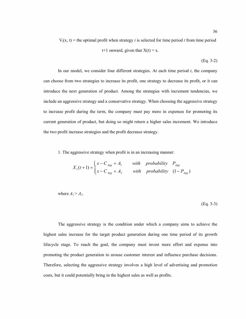
In our model, we consider four different strategies. At each time period t, the company
can choose from two strategies to increase its profit, one strategy to decrease its profit, or it can
introduce the next generation of product. Among the strategies with increment tendencies, we
include an aggressive strategy and a conservative strategy. When choosing the aggressive strategy
to increase profit during the term, the company must pay more in expenses for promoting its
current generation of product, but doing so might return a higher sales increment. We introduce
the two profit increase strategies and the profit decrease strategy.
1. The aggressive strategy when profit is in an increasing manner:
)1()1(
2
11
AggAgg
AggAgg
PyprobabilitwithACxPyprobabilitwithACx
tX
where A1 > A2.
(Eq. 3-3)
The aggressive strategy is the condition under which a company aims to achieve the
highest sales increase for the target product generation during one time period of its growth
lifecycle stage. To reach the goal, the company must invest more effort and expense into
promoting the product generation to arouse customer interest and influence purchase decisions.
Therefore, selecting the aggressive strategy involves a high level of advertising and promotion
costs, but it could potentially bring in the highest sales as well as profits.

37
Equation 3-3 indicates the potential state shifts with relative occurrence probabilities
when selecting the aggressive strategy. For the first condition, the profit increases rapidly from its
current state to a higher state than the second situation with a probability, PAgg. The following
equation, Eq. 3-4, presents the stochastic dynamic programming formulation of the optimal profit
when selecting the aggressive strategy:
)1,()1()1,(),( 211 tACxFPtACxFPtxV AggAggAggAgg
(Eq. 3-4)
2. The conservative strategy when profit is in an increasing manner:
)1()1(
2
12
ConCon
ConCon
PyprobabilitwithCCxPyprobabilitwithCCx
tX
where C1 > C2
(Eq. 3-5)
The conservative strategy is usually adopted under two market scenarios. In the first the
target product generation is still in its growth lifecycle stage, but the company is reluctant to incur
high expenses to promote that product generation. In this situation, product sales still go up but in
a mild manner. In the second scenario, the market demand is nearly saturated and there is limited
space for high sales gain. This situation usually occurs when the product generation is in its
maturity lifecycle stage. Accordingly, the company will still advertise and promote the product
generation, but it will show a lower sales increase than it would using the aggressive strategy.
Equation 3-5 indicates the two possible conditions when selecting the conservative
strategy. Profit may slightly increase from its current state with a probability, PCon. Equation 3-6
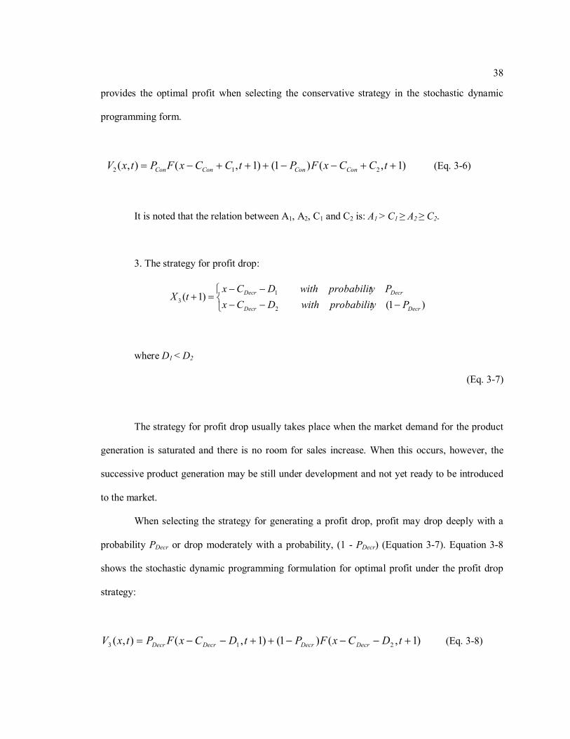
38
provides the optimal profit when selecting the conservative strategy in the stochastic dynamic
programming form.
)1,()1()1,(),( 212 tCCxFPtCCxFPtxV ConConConCon (Eq. 3-6)
It is noted that the relation between A1, A2, C1 and C2 is: A1 > C1 ≥ A2 ≥ C2.
3. The strategy for profit drop:
)1(
)1(2
13
DecrDecr
DecrDecr
PyprobabilitwithDCxPyprobabilitwithDCx
tX
where D1 < D2
(Eq. 3-7)
The strategy for profit drop usually takes place when the market demand for the product
generation is saturated and there is no room for sales increase. When this occurs, however, the
successive product generation may be still under development and not yet ready to be introduced
to the market.
When selecting the strategy for generating a profit drop, profit may drop deeply with a
probability PDecr or drop moderately with a probability, (1 - PDecr) (Equation 3-7). Equation 3-8
shows the stochastic dynamic programming formulation for optimal profit under the profit drop
strategy:
)1,()1()1,(),( 213 tDCxFPtDCxFPtxV DecrDecrDecrDecr (Eq. 3-8)

39
In addition, for each time period t, profit is constrained between a set of boundaries, Ub and Lb.
Alternatively, the company may choose to introduce the successive generation of the
product rather than to apply any of the three strategies if the current profit exceeds the threshold
H. Introducing the successive generation of a product may incur the costs of deleting the current
generation of the product. However, it may bring the company the highest return as future profit.
Since this model assumes the successive generation will completely substitute for the current
generation in the market, we also assume that at the time of its introduction, profit would drop to
its initial level. This immediate drop in profit and unrealized expected future benefits may be
regarded as unrealized profit and should be included when evaluating the corresponding optimal
profit of this strategy. Equation 3-11, Equation 3-12 and Equation 3-13 show the formulations for
these conditions. Note that Equation 3-13 indicates the company cannot choose to introduce the
successive generation if current profit does not reach the threshold H.
If HtX )( ,
ILtX )1(4 (Eq. 3-11)
DetCUPtILFtxV )1,(),(4 (Eq. 3-12)
Otherwise,
0),(4 txV (Eq. 3-13)

40
In addition, for each time period t, since F(x, t) is the maximum expected profit given that
X(t) = x, F(x, t) should be assigned the maximal expected revenue values for the following four
strategies:
F(x, t) = max {V1(x, t), V2(x, t), V3(x, t), V4(x, t)} (Eq. 3-14)
3.2 Case Study I – IBM Mainframe Systems
To verify our model, we tested it on a published case study. The data for this case is
adopted from Mahajan and Muller (1996). The systems are four successive generations of IBM
mainframe computers that appeared in the market across a 24-year timespan (1955-1978) with
sales of 301,226 units. Table 3-3 presents the adopted dataset, showing the number of systems in
use by year. We can see that the highest and the lowest volume of any single generation was
19,412 for the third generation in 1970 (highest) and 3 for the second generation in 1959 (lowest).
From Table 3-3, we observe one trait that the sales for current product generation drop
immediately when a successive product generation is introduced to the market. Rationally, the
scenario did not involve a full substitution strategy among product generations. In this case study,
since our model requires the input of data from a fully substituted MGP line, we only used the
positive sales differences between two consecutive time periods into the two increasing strategies,
which is exactly the data before the successive generation became available for each product. As
for the negative sales differences, they are set to the decrease strategy. The detailed sales
differences between every consecutive time period are shown in Table 3-4. Therefore, the
strategy settings for this case study would not conflict to the full substitution assumption.
To demonstrate our proposed methodology, we transferred this dataset into a dynamic
state model. First, we defined the number of states to use in the model. Clark and Mangel (2000)
indicated the potential for using up to 100 states. Thus, we regarded all numbers as product sales,
and we considered that using 30 states could sufficiently discriminate the sales number for each

41
year. We assumed no knowledge of unit prices and costs; accordingly, we simply used sales to
imply profit and set all costs to be 0. Therefore, in this case each state approximately equals 650
units of computer systems.
Table 3-3: The circulation data of four generations of IBM mainframe computer systems (Adopted from
Mahajan and Muller (1996))
Introduction Time Year Generation 1 Generation 2 Generation 3 Generation 4 Total
1 1955 190 190 1956 560 560 1957 1000 1000 1958 1680 1680
2 1959 2542 3 2545 1960 2640 880 3520 1961 2350 2510 4860 1962 1820 4725 6545 1963 1170 7720 8890 1964 750 10940 11690
3 1965 455 13090 625 14170 1966 303 13330 3881 17514 1967 203 9977 8125 18305 1968 170 6896 13110 20176 1969 49 4646 17687 22382 1970 29 3297 19412 22738
4 1971 14 2916 17529 806 21265 1972 6 2384 14909 2922 20221 1973 4 2079 10475 5887 18445 1974 4 1676 8060 8440 18180 1975 3 1397 6450 9335 17185 1976 1107 5919 9046 16072 1977 894 5118 10450 16462 1978 829 4641 11348 16818
Next we formulated our stochastic dynamic programming model. To solve it, we applied
backward iteration and started from the last term F(x, T). The end condition, F(x, T), was also
required for this iteration. According to Table 3-3, IBM sold 11,348 of the newest generation of
systems in 1978 and 301,226 systems in total over the entire 24 years. After transferring these
numbers into our defined states, we had x = 17 and F(17, 24) = 11,348/650 ≒ 463. Since we now
had F(17, 24) = 463, we needed a way to generate the end condition for all other states. We

42
expected the end conditions to increase from 463 as states go up from 17 and to decrease as states
move downward. To fulfill the above requirements, we developed a simple non-linear function to
derive F(x, T) for every state x. The equation for the end condition is as follows:
End Condition (EC) =
3
30171463 x
(Eq. 3-15)
Next, we defined the parameters to use in the model for the four strategies. Table 3-4
shows the yearly sales increment and decrement for each generation, achieved by calculating the
sales difference between every two consecutive years for each generation.
In Table 3-4, we can see two common features across the first three generations. First, the
sales increment suddenly shrinks before entering to the sales peak. Second, the sales decrement
becomes moderate after decreasing rapidly for several years. The fourth generation does not reach
its sales peak until 1978, thus obscuring any trends. We used regression analysis to determine
both types of increment slopes as well as the decrement slopes for these three generations. The
results are shown in Table 3-5.
In Table 3-5, we can see that sales volumes are transferred into relative shifts in states.
We identified the steep increase in sales as the aggressive increase strategy, the moderate increase
as the conservative increase strategy, and both the steep decrease and moderate decrease as the
decrease strategy. By selecting only the extreme value, we now had (A1, A2, C1, C2, D1, D2) = (7,
1, 3, 0, 0, 4). As for the probabilities of PAgg, PCon and PDecr, we used PAgg = 0.5, PCon = 0.33 and
PDecr = 0. 67 based on the occurrence tendencies from Table 3-5.
As for the strategy of introducing a newer product, IBM issued successive generations of
its mainframe system in 1959, 1965, and 1971, where the sales of the then-current generation
reached 2,542, 13,090 and 17,529, respectively. However, the sales level of the first generation

43
when introducing the second generation was significantly lower than those for the other two
generations; hence, in our model we used the sales level of the second generation for the year in
which the third generation comes to the market as our introduction threshold, H. Thus, H is set as
state 20. First year sales for every generation of product ranged from 3 to 806, so we set the initial
sales level as state 1. As for the unrealized profit, we needed to use a value higher than state 19;
thus, we simply set UP = 25. In addition, the Ub and Lb for each was state 30 and state 1.
Table 3-4: Sales increment/decrement analysis for each generation
Gen. 1 Sales (+/-) Gen. 2 Sales (+/-) Gen. 3 Sales (+/-) Gen. 4 Sales (+/-) 190 560 +370 1000 +440 1680 +680 2542 +862 3 2640 +98 880 +877 2350 -290 2510 +1630 1820 -530 4725 +2215 1170 -650 7720 +2995 750 -420 10940 +3220 455 -295 13090 +2150 625 303 -152 13330 +240 3881 +3256 203 -100 9977 -3353 8125 +4244 170 -33 6896 -3081 13110 +4985 49 -121 4646 -2250 17687 +4577 29 -20 3297 -1349 19412 +1725 14 -15 2916 -381 17529 -1883 806 6 -8 2384 -532 14909 -2620 2922 +2116 4 -2 2079 -305 10475 -4434 5887 +2965 4 0 1676 -403 8060 -2415 8440 +2553 3 -1 1397 -279 6450 -1610 9335 +895
1107 -290 5919 -531 9046 -289 894 -213 5118 -801 10450 +1404 829 -65 4641 -477 11348 +898
To solve this model, we wrote a program called the “Multiple-Generation Product Line
Simulator” using Excel VBA. The VBA code for the program is provided in Appendix A. Figure
3-1 illustrates the interface of the program, and Figure 3-2 shows the output result from the
program. Figure 3-2 indicates the optimal strategy that should be implemented at every state for
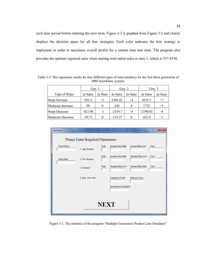
44
each time period before entering the next term. Figure 3-3 is graphed from Figure 3-2 and clearly
displays the decision space for all four strategies. Each color indicates the best strategy to
implement in order to maximize overall profits for a certain time and state. The program also
provides the optimal expected sales when starting with initial sales at state 1, which is 537.8530.
Table 3-5: The regression results for four different types of sales tendency for the first three generation of IBM mainframe systems
Gen. 1 Gen. 2 Gen. 3
Type of Slope In Sales In State In Sales In State In Sales In State
Steep Increase 582.4 +1 2306.82 +4 4335.3 +7
Moderate Increase 98 0 240 0 1725 +3
Steep Decrease -423.96 -1 -2539.7 -4 -2790.03 -4
Moderate Decrease -30.71 0 -319.57 0 -622.8 -1
Figure 3-1: The interface of the program “Multiple-Generation Product Line Simulator”

45
Figure 3-2: The output strategy map from the program “Multiple-Generation Product Line Simulator”
Figure 3-3: The decision space for each of the four strategies

46
To predict the possible moves of the MGP line according to the optimal strategy map
generated by our model, we applied the Monte Carlo forward iteration to simulate the lifetime of
this MGP line. The algorithm for this iteration is as follows:
1. At time t = 1, start at the initial state, which is state 1 in this case.
2. Move following the optimal strategies shown in Figure 3-2. If the best strategies are
strategy 1 to 3, generate a random variable r, where 0 ≤ r ≤ 1.
a. If the best strategy is strategy 1:
i. If r ≤ PAgg, then X(t+1) = X – CAgg + A1
ii. If r > PAgg, then X(t+1) = X – CAgg + A2
b. If the best strategy is strategy 2:
i. If r ≤ PCon, then X(t+1) = X – CCon + C1
ii. If r > PCon, then X(t+1) = X – CCon + C2
c. If the best strategy is strategy 3:
i. If r ≤ PDecr, then X(t+1) = X – CDecr - D1
ii. If r > PDecr, then X(t+1) = X – CDecr - D2
3. If the best strategy is strategy 4, then set X(t+1) = 1.
After simulating the iteration, we acquired a set of product line life cycle prediction
results. We again used Excel VBA and created a new program called the “Monte Carlo Forward
Iteration Simulator” to perform the iteration on existing optimal strategies. The program code is
provided in Appendix B. Figure 3-4 illustrates the predicted product line life cycle generated
from the iteration, showing that there are four generations of the product, and that the successive
generations are introduced to the market in years 5, 12 and 18.

47
0
5
10
15
20
25
30
1 3 5 7 9 11 13 15 17 19 21 23
Time
Sta
te
Figure 3-4: A simulated product line life cycle from the Monte Carlo forward iteration
To validate the forecasting performance of our proposed model, we compared our results
to those from Mahajan and Muller (1996). We first compared our lifetime predictions to Mahajan
and Muller’s and to the real data. We set the introduction years matching the real data as years 1,
6, 11 and 17, and then ran 50 Monte Carlo forward iterations based on the strategy map in Figure
3-2. We removed 23 unfeasible simulated predictions that included unexpected introduction years.
For the remaining 27 predictions, we calculated the average states for each year. The comparison
of our simulated results, the diffusion and substitution model output from Mahajan and Muller
(1996), and the real data is shown in Figure 3-5. Note that we transferred all volumes of the
mainframe systems from Mahajan and Muller and the real data into relative states, and we
revealed only the volume data before the introduction of each successive product generation.
Gen.1 Gen.2 Gen.3 Gen.4

48
0
5
10
15
20
25
30
35
1 2 3 4 5 6 7 8 9 10 11 12 13 14 15 16 17 18 19 20 21 22 23 24
Diffusion
Real
DSVM
Figure 3-5: The comparison of lifetime predictions among our simulated result, the real data and the output
from the diffusion and substitution model.
In Figure 3-5, we can see that for the entire second generation and the first four years of
the fourth generation, our simulated lifetime prediction was fairly close to the real data.
Interestingly, the diffusion and substitution model did not provide the same level of accuracy as
our model. However, for the first and the third product generation, the model output from
Mahajan and Muller (1996) generated a better prediction than our approach.
Next we compared the acquired introduction years for the third and the fourth generation
from the iteration to real data and the optimal introduction years suggested by Mahajan and
Muller (1996). We used the iteration to simulate 50 product line lifecycles, and selected only
those lifecycles that included four generations of the product. The introduction years for the third
and the fourth product generations for the 24 remaining product line lifecycles are summarized in
Table 3-6 and Table 3-7. For each generation, we calculated the weighted-sum for each year,
added up all the weighted-sum values, divided the acquired value by 24, and then rounded it up to
the nearest integer value. The average introduction years of our proposed model for the third and
the fourth generation of the product are year 12 (1966) and year 18 (1972). Table 3-8 illustrates

49
the direct comparison between our results to the optimal results from Mahajan and Muller and to
the real data.
Table 3-6: The best introduction year for introducing generation 3
The Best Introduction Year for Introducing Generation 3 Year Times Weight sum
9 (1963) 3 27 10 (1964) 3 30 11 (1965) 4 44 12 (1966) 3 36 13 (1967) 6 78 14 (1968) 4 56 15 (1969) 1 15
Average Year 11.9166667
Table 3-7: The best introduction year for introducing generation 4
The Best Introduction Year for Introducing Generation 4 Year Times Weight sum
13 (1967) 1 13 14 (1968) 0 0 15 (1969) 1 15 16 (1970) 4 64 17 (1971) 3 51 18 (1972) 5 90 19 (1973) 8 152 20 (1974) 2 40
Average Year 17.7083333
Table 3-8: Comparison between the proposed model, Mahajan and Muller (1996) and the real data
Introduction Year for Generation 3 Introduction Year for Generation 4 Proposed model 1966 1972
Mahajan and Muller (1996) 1963, 1964 1969, 1970 Real data 1965 1971
From Table 3-8, we can see that our proposed method generated a set of years which are
both only one year off from the actual introduction years. Mahajan and Muller (1996) used
different parameters and generated two pairs of optimal introduction years. In one pair, both
results are two years earlier than the real data (1963, 1969), and in the other, both are one year

50
earlier (1964, 1970). In point of fact, identifying which prediction was better is difficult since we
do not have detailed revenue information to apply further financial analysis. However, our
approach has several advantages over that of Mahajan and Muller's. First, our proposed
framework can automatically generate introduction years for every product generation. Mahajan
and Muller’s model requires repetitive optimization procedures for the current and the successive
product generation to determine the introduction time for each generation; additionally, the input
parameters for every optimization procedure need to be generated separately. Thus, our model is
intuitive and less time-consuming when generating introduction timings than Mahajan and
Muller’s model. Second, our approach has much less computational complexity. Compared to
Mahajan and Muller’s method, which requires additional in-depth information input and multiple
differential equations to achieve optimal introduction timings, our proposed approach is based on
stochastic dynamic programming and requires relatively low computation complexity.
In addition, we do an additional sensitivity analysis on five different introduction
threshold (H) settings to see how would the introduction states vary with time. The result is
shown in figure 3-6.
14
16
18
20
22
24
26
1 2 3 4 5 6 7 8 9 10 11 12 13 14 15 16 17 18 19 20
H = 16
H = 18
H = 20
H = 22
H = 24
Figure 3-6: The introduction states from different introduction threshold settings

51
We can see that since we consider H has a constant value, the introduction states remain
the same value as the H setting most of the time. However, when H is equal or higher than State
20 at t = 20, introducing a successive product generation becomes much stricter since the
introduction states all jump up to State 25. In addition, when time is over t = 20, the product line
lifetime is close to the end and introducing a successive product generation is no longer an ideal
strategy to apply.
In this case study, we input only approximate data to achieve the acceptable results
shown above. Further sensitivity analyses on parameters are still required to see how we can
better predict the actual data and how parameter settings affect the results. We try different ways
to generate values used in every strategy, and we apply different settings to formulate the end
condition.

52
Chapter 4
Methodology (II) – The Cannibalization Scenario
In this chapter, we introduce the proposed methodology with the second scenario,
which entails cannibalization. In it, MGPs compete simultaneously in the same market. The
cannibalization model is introduced in Section 4.1. Using this model, we consider two types
of applications. For the first, the cannibalization model is applied to forecast the lifetime
performance of an on-going MGP line based on limited existing sales data. This application is
discussed in Section 4.2. For the second application, presented in Section 4.3, the same model
is applied to forecast the lifetime performance of a brand new product line not yet introduced
to the market, using the sales data of a similar existing product line. In Section 4.4, we
introduce the technology evolution model, in which cannibalization is incorporated with
technology evolution concern.
4.1 Model Construction
Like the full substitution scenario, the cannibalization model includes two stages. For
the first, we formulated a DSVM to predict the sales behaviors of the entire MGP line. With
the solution of the DSVM, we obtained strategy maps for the product line, identifying the best
time-state strategy for any given product generation to adopt within the entire product line
lifecycle. We consider these strategy maps to be the core value for applying DSVMs on MGP
lines. They directly indicate the best strategic move for a company to adopt at each time and
market state to achieve the highest profits. For the second stage, we applied Monte Carlo
forward iteration to simulate predicted lifecycle performances for the MGP line. In this
chapter, unlike in Chapter 3, we have moved the setting explanation of the iteration to an
independent sub-section that follows formulation of the model. There are two reasons for this

53
move. First, we modified the settings and procedures of the typical Monte Carlo forward
iteration to work with the cannibalization scenario. Second, the modified iteration is
repetitively applied throughout all the sections in this chapter.
4.1.1 The Cannibalization Model
The core of the cannibalization model is the DSVM. The model is based on the
following assumptions. First, we assume a company plans to launch a new multi-generation
product line to the market between a certain time interval t = 1 to t = T. Second, from time
period t to t+1, sales of each product generation currently in the market may either increase or
decrease, following a stochastic process based on the strategy it selects. Third, all moves are
based on pre-determined rules. In a DSVM, the objective is not assumed to be moving
randomly but acting within the preselected strategies. Fourth, each product generation is
independent from every other in sales tendency. Fifth, cannibalization occurs among product
generations; that is, when the company releases a new generation of the product, the existing
product generations are not withdrawn from the market, and multiple generations of the
product may coexist in the same market, lessening each others’ profit. Sixth, when a
successive generation comes into the market, the existing product generations no longer grow
in sales but rather start to decay. Seventh, the overall sales behavior of the MGP line is
assumed to be symmetric across the time period, (T+1)/2. This assumption is derived from
both the diffusion of innovations by Rogers (1995) and observations from real product lines.
Rogers (1993) indicated that the distribution of the adoption of innovations by individuals
follows a bell-shaped curve. In addition, we observed the sales behaviors of several
terminated or still on-going MGP lines (e.g., IBM Mainframe systems, Apple iPhones, etc.)
and found that both the life cycle sales for every individual product generation and the overall
product lines approach a symmetric bell-shaped. And the last, every product generation is
assumed to have a common unit price of 1 unit; thus, product sales volume can directly
represent revenue. Table 4-1 includes all the parameters we used in the DSVM. In our model,

54
we used one DSVM with mixed strategies, including both sales increase and sales decrease
scenarios. However, the choice of strategy for each state and time was separate and
independent for each scenario. Therefore, each scenario had its own unique objective function
under the same state and time. As the proposed DSVM involved the cannibalization condition,
we now start introducing the cannibalization model and the various strategies involved.
To begin with the cannibalization model, we first define the expected profit function
Fi(x, t) as:
Fi(x, t) = maximum expected profit between time period t and the expected end of life of the
multiple-generation product line for sales scenario i, given that X(t)=x.
(Eq. 4-1)
In this model, since we only have two different sales scenarios (increase or decrease),
there are two cases for i. These are F1(x, t) and F2(x, t), each representing the optimal strategy
at state x in time period t of the sales increase scenario and sales decrease scenario. The actual
optimal profit of the entire product line, Fi(x,T), is acquired by summation of all the expected
profits at the last time period.
After defining Fi(x, t), we need to clarify the expected profit values corresponding to
the strategy chosen at state x and time period t, preceding time period T.
Let,
J(x, t) = the optimal profit when strategy j is selected for time period t from time
period t+1 onward, given that X(t) = x.
(Eq. 4-2)

55
Table 4-1: Cannibalization model parameters
Th(t) Threshold for introducing the successive generation of product at time period t. Unit is state.
Agg(t) Product sales when applying aggressive increase strategy at time period t. Unit is state.
PCon Probability for profit increase when applying the conservative strategy. Poscr Probability for profit increase or decrease when applying the oscillation strategy. PIntro Probability for profit decrease when applying the successive product generation
introduction strategy. PCv Probability for the rapid sales converge when applying the converge strategy. B1 The more profit increment when applying the conservative strategy. Unit is state. B2 The less profit increment when applying the conservative strategy. Unit is state. C1 The more profit increment or the less profit decrement when applying the oscillation
strategy. Unit is state. C2 The more profit decrement when applying the oscillation strategy. Unit is state. I1 The less profit decrement when applying the successive product generation
introduction strategy. Unit is state. I2 The more profit decrement when applying the successive product generation
introduction strategy. Unit is state. EP Expected profit gain under the strategy if introducing the successive generation of
product. D1 Rate of the more profit decrement when applying the decrease strategy. Unit is state. D2 Rate of the less profit increment when applying the decrease strategy. Unit is state. D3 Constant decrease rate of the convergence strategy.
CAgg Cost involved when adopting the aggressive increase strategy. Unit is state. CCon Cost involved when adopting the conservative increase strategy. Unit is state. Cosc Cost involved when adopting the oscillation increase strategy. Unit is state. CDecr Cost involved when adopting the decrease strategy. Unit is state. CCv Cost involved when adopting the converge strategy. Unit is state.
CIntro Costs involved in introducing the successive generation of product. Unit is state. T Entire (multiple-generation) product life span. Unit is season.
X(t) Amount of profit at the start of time period t. Unit is state. Cg Convergence threshold for the sales decrease scenario. Unit is state. Cv The rapid sales converge in the converge strategy. Unit is state. xcrit The critical level for product sales in sales increase model. Unit is state. ycrit The critical level for product sales in sale decrease model. Unit is state.
To construct a DSVM, it is necessary to understand the potential behaviors of the
targeted object that is modeled. These potential behaviors must be transferred into
corresponding strategies. To develop appropriate strategies, we observed the sales behaviors
of several technology-intense MGP lines (mobile phones, tablets and computers) and found
several common traits. First, the initial sales period of a product generation varies with time.
The introduction sales are normally relatively low in the first few generations and start
growing as the product line moves toward its maturity stage. After the product line passes its
peak, the introduction sales gradually decline. Second, when a product generation is in its
growth stage, sales increase substantially. Third, sales may have subtle variations during the

56
growth stage or when at the peak of sales, with either minor increments or decrements. This
situation might also occur when a company attempts to delay the introduction of the
successive generation and allows the current generation to remain in the market. Fourth, when
a successive generation is introduced to the market, sales of the previous generation
simultaneously drop significantly. Fifth, when a generation is replaced by its successor, its
sales start dropping quickly. Last, when a product generation is close to its end of life, sales
decline marginally and gradually converge to zero. We found that our observed sales traits
could be appropriately interpreted from the viewpoint of typical product life cycle stages. The
first situation could reflect a product generation in its introduction stage. The second situation,
rapid growth in sales, could reflect the conditions during the growth stage. When a product
generation enters its maturity stage, the market is saturated; product sales might reflect the
third sales situation with subtle movements or start entering the decline stage, during which
the successive generation is introduced to the market. Moreover, the last two observed sales
decay situations could be regarded as the front and rear portion of the decline stage,
respectively. Hence, we tried to form our strategies from the product life cycle point of view
by incorporating observed sales traits.
To tackle this problem, we adopted a concept proposed by Thietart and Vivas (1984).
They formulated quantitative criteria for product life cycle stages after analyzing the market
growth of 1100 businesses across a four-year period with correction for inflation. They
determined that if a business has a growth rate between 0 to 4.5%, it is in the maturity stage of
its life cycle; if the growth rate is above 4.5%, the business is in the growth stage; if the
market growth rate is negative, the business is in the decline stage of its life cycle. Note that
business growth indicates the change in total sales.
In this study, we propose six general strategies for MGP lines based on our
observations and these quantitative criteria for product life cycle stages. At each state and
time period, the company can select from among four sales increase strategies for its current

57
product generation and from two sales decrease strategies for older product generations in the
process of fading out from the market.
To model different sales tendencies, we separated the strategies into two scenarios: 1)
the sales increase scenario, and 2) the sales decrease scenario. For the sales increase scenario,
at each time period t, the company can either select from three strategies to grow or oscillate
in sales, or it can choose to introduce the successive generation. Thus, the four sales increase
strategies include an aggressive increase strategy, a conservative increase strategy, an
oscillation increase strategy and a successive product generation introduction strategy. For
the sales decrease scenario, the company may select from three sales decrease strategies
having different levels of sales drops. The three strategies include an aggressive decrease
strategy, an oscillation decrease strategy and a convergence strategy. It is noted that the six
strategies are observed from technology-intense product lines; thus, we suggest the
appropriateness of applying these strategies on product lines in technology-intense industries.
Next, we introduce the strategies of the two scenarios, respectively.
4.1.1.1 Sales Increase Scenarios
In this section, we provide further explanation on the four sales increase strategies.
1. The Aggressive Increase Strategy
Otherwise 0
1 x if)()1(1
tAggxtX
(Eq. 4-3)
The aggressive strategy is the sales performance of the first time period, when a new
generation of a product is introduced to the market. The aggressive strategy represents the
introduction stage of product life cycle. In this model, we set state 1 as the critical state and
observed that when the new generation introduction strategy is applied to the current

58
generation, the new generation is at the critical state simultaneously and waits to be
introduced to the market. In the following time period, the new generation follows the
aggressive strategy and jumps to the corresponding state. Therefore, the aggressive increase
strategy only occurs when a new generation is at state 1. In fact, the introduction sales
performance of a new generation should vary with time and the stage of the product line
lifecycle. To better fit observed real world sales conditions, we defined the sales performance
of the aggressive increase strategy as a polynomial function Agg(t), which varies with time t
and is symmetric with respect to (T+1)/2. In addition, this strategy cannot be selected when a
product generation is no longer at state 1. Equation 4-4 presents the stochastic dynamic
programming formulation of the optimal profit when selecting the aggressive strategy:
Otherwise 0
1 x If C-1) t,)1((),( Agg
1
tAggxFtxV
(Eq. 4-4)
2. The Conservative Increase Strategy
1 xIf ,
)P-(1y probabilit with
Py probabilit with )1(
Con2
Con12 Bx
BxtX
Where B1 > B2
(Eq. 4-5)
We consider the conservative increase strategy as the situation in which the product
generation has a rapid sales increase over 4.5%. This strategy is adopted when a generation is
in the growth stage of its life cycle. Equation 4-5 indicates the two possible conditions when
selecting the conservative strategy. If the current state of a generation is not at state 1, its
product sales may increase from their current state to a much higher state B1 with a
probability, PCon, or they may increase to a slightly higher state with a probability, (1 - PCon).

59
Equation 4-6 provides the optimal profit when selecting the conservative strategy in the
stochastic dynamic programming form.
OtherwiseCtBxFP
tBxFPtxV ConCon
Con
0 UB(t) xand 1 xIf )1,()1(
)1,(),( 2
1
2
(Eq. 4-6)
3. The Oscillation Increase Strategy
1 xIf ,
)P-(1y probabilit with
Py probabilit with )1(
Osc2
Osc13 Cx
CxtX
Where C1 > C2
(Eq. 4-7)
The oscillation increase strategy is defined as the condition when a product
generation enters the maturity stage of its life cycle and has a sales growth under 4.5%. We
also consider this strategy may include negative sales, which differs from the original
definition from Thietart and Vivas (1984). The reason for this twist is we observe that sales
may slightly oscillate between positive and negative growth when a generation is in its
maturity stage. Therefore, when selecting this strategy, profit may slightly increase or
decrease in the amount of C1 with a probability POsc , or it may drop moderately in the amount
of C2 with a probability, (1 - PDecr) (Equation 4-7). Note that C1 may be positive or negative,
but C2 is negative. Equation 4-8 illustrates the stochastic dynamic programming formulation
for optimal profit under the oscillation increase strategy.

60
1 xIf ,
OtherwiseCtCxFP
tCxFPtxV OscOsc
Osc
01 xIf )1,()1(
)1,(),( 2
1
3
(Eq. 4-8)
For each time period t, product sales should stand above a lower bound constraint
(xcrit). As such, xcrit is the critical level of product sales, and any generation with a state
smaller than or equal to xcrit is considered to be withdrawn from the market. As mentioned
previously, xcrit is set as state 1.
4. The Successive Product Generation Introduction Strategy
The successive product generation introduction strategy embodies the conditions
under which a successive generation enters the market while the current generation enters the
decline stage of its life cycle. Under this strategy, the company may decide to introduce the
successive product generation if the current product sales exceeds the introduction threshold,
Th(t). In this model, we assume the lifecycle of a product line is a symmetric bell-shaped
distribution. Thus, sales of a product line start growing from its introduction and peak at the
middle of the product line’s lifetime. After that, the product line enters the decline stage and
the sales drop continually toward the end of life. Realistically, the introduction threshold
should vary with the sales level rather than setting as a constant rate. Therefore in this model,
we consider the product introduction threshold is dynamic and follows a polynomial function
which varies with time and is symmetric at t = (T+1)/2. Introducing the successive generation
may incur a certain amount of introduction costs. On the other hand, it may potentially bring
the company the highest gain in return as future profit. Since our model incorporates
cannibalization, product sales for the target generation do not fall to the critical state but drop
to a pair of lower states, and eventually follow a set of stochastic probabilities when the

61
successive generation is introduced to the market. Equation 4-9 relates to the condition when
the current sales level exceeds the product introduction threshold, Th(t); the product sales may
drop I1 state with a probability of Pintro, or decrease I2 state with a probability of (1 – Pintro).
Equation 4-10 shows the stochastic dynamic programming function for optimal profit under
the successive product generation introduction strategy. In it, EP is the expected profit gain
when introducing the successive generation. However, if current sales are within the threshold,
the company should opt not to introduce the successive generation since doing so would not
benefit the company in the long run but might significantly harm its profitability.
)( tThxIf ,
)P-(1y probabilit with
Py probabilit with )1(
Intro2
Intro14 Ix
IxtX
Where 0 > I1 > I2
(Eq. 4-9)
Otherwise 0
Th(t) If)]1,()1()1,([),( 21
4
xCtIxFPtIxFPEPtxV IntroIntroIntro
(Eq. 4-10)
For each time period t, since F1(x, t) is the maximum expected profit given that X(t) =
x, F1(x, t) should be assigned the maximal expected revenue value for the above four
strategies in the sales increase scenario:
F1(x, t) = max {V1(x, t), V2(x, t), V3(x, t), V4(x, t)}
(Eq. 4-11)
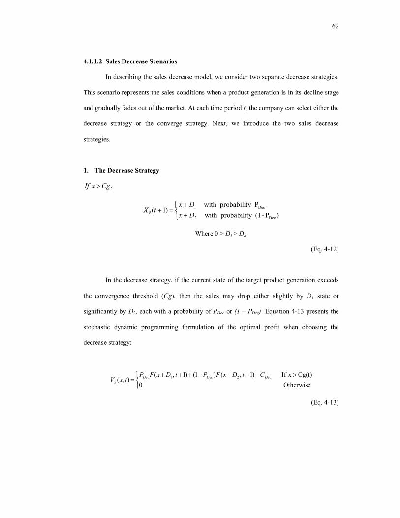
62
4.1.1.2 Sales Decrease Scenarios
In describing the sales decrease model, we consider two separate decrease strategies.
This scenario represents the sales conditions when a product generation is in its decline stage
and gradually fades out of the market. At each time period t, the company can select either the
decrease strategy or the converge strategy. Next, we introduce the two sales decrease
strategies.
1. The Decrease Strategy
CgxIf ,
)P-(1y probabilit with
Py probabilit with )1(
Dec2
Dec15 Dx
DxtX
Where 0 > D1 > D2
(Eq. 4-12)
In the decrease strategy, if the current state of the target product generation exceeds
the convergence threshold (Cg), then the sales may drop either slightly by D1 state or
significantly by D2, each with a probability of PDec or (1 – PDec). Equation 4-13 presents the
stochastic dynamic programming formulation of the optimal profit when choosing the
decrease strategy:
Otherwise 0
Cg(t) xIf)1,()1()1,(),( 21
5DecDecDec CtDxFPtDxFP
txV
(Eq. 4-13)

63
2. The Convergence Strategy
CgxIf ,
)()1( 36 txDtX
Otherwise
)P-(1y probabilit with Py probabilit with )(
)1(Cv
Cv36 Cvx
txDtX
(Eq. 4-14)
We define “convergence” as the condition when the product sales gradually move
toward “zero” sales and the target product generation is about to be removed from the market.
We consider convergence includes two scenarios. In the first, when product sales are above
the convergence threshold (Cb), they slowly converge. We assume sales no longer drop by
constant states but diminish following a certain discount rate. In the second scenario, when
the current state is equal to or lower than the convergence threshold (Cb), sales drop in two
different ways. They may rapidly converge by Cv states with a probability of PCon, or they
may still drop following the same discount rate with a probability of (1-PCon). This scenario
represents the situation where a product generation is approaching its end of life, at which
time the company may either retain it in the market or directly withdraw it. When the current
state of a product generation is lower than the critical state, it is removed from the market.
Equation 4-15 provides the optimal profit when selecting the convergence strategy in the
stochastic dynamic programming form.
CgxIf ,
Cg xIf C- )1),((),( Cv36 ttxDFtxV

64
Otherwise
1 CvxIf
Cv36 C- )1),(()1()1,)((),( ttxDFPtCvtxFPtxV ConCon
(Eq. 4-15)
For each time period t, since F2(x, t) is the maximum expected profit X(t) = x, F2(x, t)
should be assigned the maximal expected revenue values for the above two strategies in the
sales decrease scenario:
F2(x, t) = max {V5(x, t), V6(x, t)}
(Eq. 4-16)
After formulating this cannibalization model, backward iteration is used to solve it.
We start from the last term t = T and move backward in time. Thus, the end condition Fi(x,T),
the total expected future profit for the product line, must be given. We assume Fi(x, T) is a
function K(x), and we define it in the case study section.
The cannibalization model outputs two optimal time-state strategy maps for both
scenarios, indicating the optimal strategy to apply for a targeted product generation at each
time and state under either of the two sales scenarios. Tactic-wise, these strategy maps allow
the company to develop long-term product line strategies or to adjust its strategies toward
dynamic market changes.
In this section, we propose six strategies considering product lifecycle stages to use in
the dynamic variable model. These strategies look only at the typical movements a product
generation normally engages in according to its lifecycle stage in the market. Companies can
develop alternate strategies, incorporating their specific requirements or concerns. For this
study, we only simplify the complexity of pricing by setting an equal unit price across all

65
strategies. Companies can set strategies with product unit prices to determine which should be
applied at different states and times, and can input a distinct setting of strategies into the
model to verify and ensure their market tactics.
4.1.2 Monte Carlo Forward Iteration
Having defined the cannibalization model, we proceed to the second stage, the Monte
Carlo forward iteration. The reason for conducting the iteration at this point is to generate the
lifecycle predictions of the MGP line based on output from the strategy maps output of the
cannibalization model. The simulated lifecycles generated by this iteration can be regarded as
the optimized lifecycle prediction for the target MGP line, based on the pre-determined input
strategies which include the observed terms of sales trend.
Typically the Monte Carlo forward iteration simulates the behavior of an object
throughout the entire observation duration. In this study, we apply a modified version to
simulate the behaviors of all generations in a product line within the product line lifecycle.
The simulation process starts from the beginning of the first generation at t = 1. For
generation k, when the successive t generation introduction strategy is adopted, product
generation k+1 emerges in the market and generation k starts to decay. When a product
generation is in its growth, we refer to the strategy map from the sales increase scenario.
Otherwise, we consult the strategy map from the sales decrease scenario. The algorithm of the
Monte Carlo forward iteration for this study is explained next.
To begin with, generate a random variable r, where 0 ≤ r ≤ 1. Let xk and x'k to
represent the integer state and the real state of product generation k at time t, respectively.
The difference between xk and x'k is that xk is the integer portion of the x'k. For a product
generation that is between states s and s+1 at time t, we consider that the product generation
should follow the best strategy of the integer portion of its actual state, which is state s, since
it does not actually stand on state s+1. However, when considering its future move, we still
use its real state to decide the potential changes in states. Moreover, let yk be the market

66
entrance time for product generation k, and y1 = 1. Below, we show the decision process for
the Monte Carlo forward iteration applied in this case.
1. At time t = 1, the iteration starts from product generation 1. x1 = 'kx = )1(Agg . We
choose the integer part of the real state Agg(1) as our initial state.
2. Find the optimal strategy from the sales increase scenario, which is F1(xk, t) = i for
product generation k. Action taken follows the optimal strategy.
3. If i = 1, then follow the aggressive increase strategy. x'k = Agg(t), xk = 'kx . If t = tmax,
end simulation. Otherwise, t = t +1 and go to step 2.
4. If i = 2, then follow the conservative increase strategy:
a. If r ≤ PCon, then x'k = x'k + B1, xk = 'kx .
b. If r > PCon, then x'k = x'k + B2, xk = 'kx .
If t = tmax, end simulation. Otherwise, t = t +1 and go to step 2.
5. If i = 3, then follow the oscillation increase strategy:
a. If r ≤ POsc, then x'k = x'k + C1, xk = 'kx , z'k = z'k + C1.
b. If r > POsc, then x'k = x'k + C2, xk = 'kx , z'k = z'k + C2.
If t = tmax, end simulation. Otherwise, t = t +1 and go to step 2.
6. If i = 4, then follow the new product introduction strategy:
a. If r ≤ PIntro, then x'k = x'k + I1, xk = 'kx .
b. If r > PIntro, then x'k = x'k + I2, xk = 'kx .

67
If t = tmax, end simulation. Otherwise, t = t +1, xk+1 = x'k+1 = 1, yk+1 = t+1. Go to step
6.
7. Find the optimal strategy from the sales decrease scenario, which is F2(xk, t) = j for
product generation k. Moving follows the optimal strategy.
8. If j = 5, then follow the converge strategy. If xk > Cg, then x'k = x'k * D3 and xk = 'kx .
Otherwise,
a. If r ≤ PCv, x'k = x'k – Cv, xk = 'kx .
b. If r > PCv, x'k = x'k * D3, xk = 'kx .
9. If xk < 1, the end simulation because the product generation is lower than the critical
state and is withdrawn from the market. t = yk + 1, k = k + 1, and go to step 2. If t =
tmax, end simulation. Otherwise, t = t + 1 and go to step 6.
Using the Monte Carlo forward iteration, the system automatically generated the
necessary generations of products based on the decision maps of the two scenarios output
from the DSVM. We recorded all xk during the simulation procedure, and acquired the
lifecycle prediction of the entire MGP line by depicting all the xk values in the end of the
simulation.
In the next section, we provide an illustrative case study implementing the
cannibalization model on an on-going MGP line – Apple Inc.’s iPhone product line.
4.2 Case Study II: Forecasting an On-going Multiple-generation Product Line
In this section, we describe our attempt to implement the proposed framework on an
on-going real world MGP line. We chose Apple Inc.’s famous product line, the Apple

68
iPhones, as our objective. The iPhone product line is a very typical MGP line. The iPhones
are introduced to the market one after another in a sequence, retaining the same core functions,
and updating the improved or up-to-date technologies in newer models. For instance, between
the first and fourth generations of the iPhone, the designers continually improved various
aspects of the product including mobile network transmission speed, screen resolution, CPU
speed, ram capacity, and camera pixels.
Since 2007, Apple Inc. has released five generations of iPhones and sold more than
200 million units globally. Table 4-2 provides quarterly sales statistics for the Apple iPhone
product line until 2012 third quarter (Q3), acquired from Wikipedia. In this case study, we try
to implement the proposed framework using the first 17 terms of sales from Table 3 to
forecast the lifetime sales behavior and successive product generation introduction timings for
the entire iPhone product line. Figure 4-1 is graphed based on the sales figures provided in
Table 4-2, but includes the generation information. We can observe the four generations of
iPhones. In Figure 4-1, we see that during certain quarters, more than one generation was in
the market. Overlapping generations are marked with equal sales because Apple Inc. does not
disclose distinguishable sales information for individual generations when multiple
generations are competing simultaneously in the market.
Table 4-2: Sales statistics for the Apple iPhone product line as of June 2012 (Wikipedia. http://en.wikipedia.org/wiki/File:IPhone_sales_per_quarter_simple.svg)
Fiscal Year Q1 (Oct-Dec) Q2 (Jan-Mar) Q3 (Apr-Jun) Q4 (Jul-Sep) Total Sold 2007 270,000 1,119,000 1,389,000 2008 2,315,000 1,703,000 717,000 6,890,000 11,625,000 2009 4,363,000 3,793,000 5,208,000 7,367,000 20,731,000 2010 8,737,000 8,752,000 8,398,000 14,102,000 39,989,000 2011 16,240,000 18,650,000 20,340,000 17,070,000 72,300,000 2012 37,040,000 35,100,000 26,000,000 98,140,000
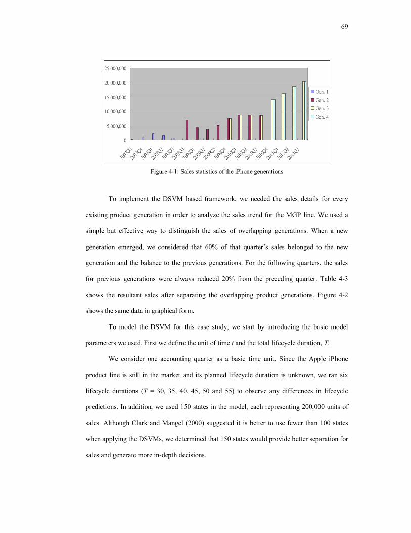
69
0
5,000,000
10,000,000
15,000,000
20,000,000
25,000,000
2007
Q320
07Q4
2008
Q120
08Q2
2008
Q320
08Q4
2009
Q120
09Q2
2009
Q320
09Q4
2010
Q120
10Q2
2010
Q320
10Q4
2011
Q120
11Q2
2011
Q3
Gen. 1
Gen. 2
Gen. 3
Gen. 4
Figure 4-1: Sales statistics of the iPhone generations
To implement the DSVM based framework, we needed the sales details for every
existing product generation in order to analyze the sales trend for the MGP line. We used a
simple but effective way to distinguish the sales of overlapping generations. When a new
generation emerged, we considered that 60% of that quarter’s sales belonged to the new
generation and the balance to the previous generations. For the following quarters, the sales
for previous generations were always reduced 20% from the preceding quarter. Table 4-3
shows the resultant sales after separating the overlapping product generations. Figure 4-2
shows the same data in graphical form.
To model the DSVM for this case study, we start by introducing the basic model
parameters we used. First we define the unit of time t and the total lifecycle duration, T.
We consider one accounting quarter as a basic time unit. Since the Apple iPhone
product line is still in the market and its planned lifecycle duration is unknown, we ran six
lifecycle durations (T = 30, 35, 40, 45, 50 and 55) to observe any differences in lifecycle
predictions. In addition, we used 150 states in the model, each representing 200,000 units of
sales. Although Clark and Mangel (2000) suggested it is better to use fewer than 100 states
when applying the DSVMs, we determined that 150 states would provide better separation for
sales and generate more in-depth decisions.

70
Table 4-3: Sales per product generations
Period Quarter Gen. 1 Gen. 2 Gen. 3 Gen. 4 1 2007Q3 270,000 2 2007Q4 1,119,000 3 2008Q1 2,315,000 4 2008Q2 1,703,000 5 2008Q3 717,000 0 6 2008Q4 0 6,890,000 7 2009Q1 4,363,000 8 2009Q2 3,793,000 9 2009Q3 5,208,000 0 10 2009Q4 2946800 4420200 11 2010Q1 2357440 6,379,560 12 2010Q2 1885952 6,866,048 13 2010Q3 1508762 6,889,238 0 14 2010Q4 0 5640800 8461200 15 2011Q1 4512640 11,727,360 16 2011Q2 3610112 15,039,888 17 2011Q3 2888090 17,449,910
0
2000000
4000000
6000000
8000000
10000000
12000000
14000000
16000000
18000000
20000000
2007
Q4
2008
Q2
2008
Q4
2009
Q2
2009
Q4
2010
Q2
2010
Q4
2011
Q2
Gen. 1
Gen. 2
Gen. 3
Gen. 4
Figure 4-2: Sales trends for individual generations
Strategies need to be determined next. For this case study, we analyzed the data from
Table 4-3 and decided to use five strategies: all four strategies from the sales increase
scenario plus the convergence strategy from the sales decrease scenario. The reason we
excluded the decrease strategy is because the way we separate the sales data is the exact same
way we set the convergence strategy. Thus, for this case study, it is not necessary to use the
decrease strategy.
The value settings for the five strategies were based on the following rules. First, all
introduction sales for each generation of iPhone were taken into account when determining

71
the aggressive strategy. Second, if the sales growth between two consecutive time periods was
above 4.5% and at the same time the successive generation was not yet in the market, all sales
except the introduction sales in Table 4-3, belonged to the conservative increase strategy.
Third, if the sales growth between two consecutive time periods was less than 4.5% and at the
same time the successive generation was not yet in the market, we considered it to represent
the oscillation strategy. Last, during the time period the successive generation was introduced
to the market, sales drops were set to the successive product generation introduction strategy.
In addition, for strategies involving probabilities, we first calculated the mean for all sales
within each strategy. Next, we calculated the sub-means for sales beyond and beneath the
mean relatively to acquire the higher and lower values used in each strategy. We also
calculated the number of sales beyond and beneath the mean divided by the total number of
sales within each strategy to obtain the relative probabilities.
Table 4-4 shows the settings for three strategies (conservative increase, oscillation
increase and successive product generation introduction) where the unit is the state. The
successive introduction strategy is more complicated than the other two. Table 4-4 reveals
only the potential sales variations when applying this strategy; we still need to consider two
critical parameters. One is the introduction threshold function (Th(t)) and the other is the
expected profit gain (EP). The first, Th(t), is a symmetric function. We chose all preceding
time periods as observation points, and we set the mildest slope between the sales volume of
the latest observation point to all the other points to be Th(t). The detailed slope and intercept
values for Th(t) are shown in Table 4-5. As for the EP, we simply define it as the sales
increment rate between the total sales in the time period where a successive product
generation is introduced to the market over the total sales in the previous quarter. We connect
all the EP ratios we observed from the data in Table 4-3, and assume EP is linear and varies
with time as well.
The other strategies, which are not included in Table 4-4, are the aggressive strategy
and the convergence strategy. For the latter, we set the converge rate (D3) = 0.8, the

72
convergence threshold (Cg) as state 7.54, and the rapid convergence rate (Cv) = 5.56 states.
For the aggressive strategy, we used the time and sales differences between the first and
fourth generations of iPhones at the each of its introduction time period to generate the slope
and intercept for t ≤ (T+1)/2, and use symmetric settings for t > (T+1)/2. The detailed slopes
and intercepts of the aggressive strategy can be seen in Table 4-5. In addition, the
cannibalization model assumed costs only relate to the sales increase strategies. We set the
cost of using the successive introduction strategy at 10 states of product sales amount, and set
the cost at 1 state for other strategies to sufficiently discriminate the cost differences.
Table 4-4: Settings for three of the strategies
Strategy Parameter Increase Rate Probability B1 11.19 0.625 Conservative Increase Strategy B2 7.42 0.375 C1 1.00 0.200 Oscillation Increase Strategy C2 -5.87 0.800 I1 -6.24 0.500 Successive Product Generation Introduction Strategy I2 -11.31 0.500
Table 4-5: Parameter settings for the three time-dependent symmetric functions
For t ≦(1+t)/2 For t ≧(1+t)/2 Function Slope Intercept Slope Intercept
Agg(t) 3.15 -1.80 -3.15 127.37 Th(t) 2.10 7.13 -2.10 93.29
The total expected future sales K(x) needs to be given in order to solve the
cannibalization model. We assumed the iPhone product line sells 100 states of units per time
period. We further supposed that the sales variance would be 20%. T is the total lifecycle
duration, x indicates the state, and unit profit margin is U. Thus, K(x) will be:
TUxTUxUT
UTxK
33.333,53000,000,16 ]150/)22.0(000,200100[
8.0000,200100)(
(Eq. 4-17)

73
After defining all the model settings, strategies and boundaries used in this case study,
we ran the cannibalization model followed by the Monte Carlo forward iteration with our
Excel-VBA based program. The code for the program can be seen in Appendix C. Figure 4-3
includes six simulated lifecycles based on different lifecycle durations for the iPhone product
line. The cannibalization model outputs two strategy maps from both of the sales scenarios,
and Figure 4-4 is the strategy map derived from the sales increase scenario. In Figure 4-4, the
x-axis is time and y-axis is state, and each color represents a sales increase strategy to be
applied at a certain time and state.
Figure 4-3: The simulated iPhone product line lifecycles

74
Figure 4-4: The strategy map of the sales increase scenario output from the cannibalization model
4.2.1 Model Validation
To see the introduction timing prediction performance between our proposed
framework and the real data, we ran 50 iterations for each lifecycle durations and calculated
the average introduction timing for every product generation in each of the six trials. Table 4-
6 includes the average output results and the real introduction quarters of the iPhone product

75
line. In Table 4-6, we can see that the actual fifth and sixth generations of iPhones were
released in the 19th and 22th quarter; the results are close to our predicted lifecycle durations of
30 quarters. Additionally, we can see one common trait in Table 4-6: the longer the planned
product line lifecycle duration, the longer the individual lifecycle span for those generations
released near the center of the entire duration. For example, from T = 30 to T = 55, the
duration span becomes longer between the generation 4 and 5 and between generations 5 and
6. This feature can be easily explained. When a product line is in the center of its lifecycle
duration, it is usually at the maturity stage. At this time, the sales volume is usually at peak
levels and market demands are considerably stable. Thus, the company should sustain the
current product generation in the market for a longer time to extend the benefits and increase
its market share.
The introduction timing output from the cannibalization model is an average value
drawn from 50 simulated lifecycles. If a company followed the strategy maps, it might have a
different lifecycle behavior based on the stochastic model setting. The optimal strategy at
each time and state provided in each strategy maps is the most profitable strategy that could
benefit companies in the long-run. If companies have distinct concerns or market plans,
applying non-optimal strategy is also workable. But it only indicates that this move will not
result in the highest profits.
Table 4-6: The six sets of average successive product generation introduction timings from six different product line lifecycle durations comparing to real Apple iPhone multiple-generation product line
Gen 1 Gen2 Gen 3 Gen 4 Gen 5 Gen 6 Gen 7 Gen 8 Gen 9 Gen 10 Gen 11 T = 30 1 6 8 14 19.12 23.1 26.1 28.4 T = 35 1 6 8 14 21.1 25.32 28.82 31.82 34.16 T = 40 1 6 8 14 23.06 28.04 32.04 35.16 38.04 T = 45 1 6 8 14 25.04 30.54 35.04 38.7 41.7 44.1 T = 50 1 6 8 14 25.1 31.66 36.78 40.84 44.36 47.36 49.51 T= 55 1 6 8 14 25.18 32.94 38.86 43.74 47.7 50.76 53.26 Actual 1 6 10 14 19 22
In addition, we performed two additional sensitivity analyses. For the first sensitivity
analysis, we test different settings of the expected profit gain (EP) to see how value changes

76
would impact introduction timings. Originally we set EP as a linear connection between every
pair of sales increase ratios when the successive product generation was introduced to the
market. As shown in Table 4-7, we tested different settings of EP, from the original dynamic
value changing with time to constant threshold value. We can see that changes in EP would
significantly affect the introduction decisions for successive product generations. In the
original setting, EP ranges from the lowest value 1.415 to the highest value 9.609. Thus,
changing in EP not only influences the introduction timing for a certain product generation,
but also impacts the introduction decisions for the entire product line.
Table 4- 7: The sensitivity analysis for the expected profit gain (EP)
Gen 1 Gen2 Gen 3 Gen 4 Gen 5 Gen 6 Gen 7 Gen 8 Gen 9 Linear Connection 1 6 8 14 23.14 28.16 32.16 35.32 38.06
Constant Threshold Value Average (EP = 4.234) 1 11.4 18.44 25.24 29.82 33.54 36.54 38.82 Highest (EP = 9.609) 1 10.84 16.72 20.78 24.26 28.4 32.44 35.66 38.14 Lowest (EP = 1.415) 1 17.36 24.54 29.38 33.26 36.26 38.74
For the second sensitivity analysis, we attempted to investigate the assumption about
the introduction threshold (H). In the cannibalization model, we assume the introduction
threshold is a symmetric function where t = (T+1)/2. Here we compare four different settings
of H to see the impact on introduction timings. The four different H settings are: 1) original
assumption (symmetric setting), 2) non-symmetric setting, 3) symmetric threshold generated
from regression, and 4) non-symmetric threshold generated from regression. The results for T
= 40 are shown in Table 4-8. It is noted that for the non-symmetric threshold settings, the
threshold values increase progressively as time moves on. Therefore, introducing a successive
product generation becomes more and more difficult in the latter stages of the product line
lifecycle. Besides, we can see that the symmetric threshold generated from the regression
output provides a very close prediction as the original threshold setting.
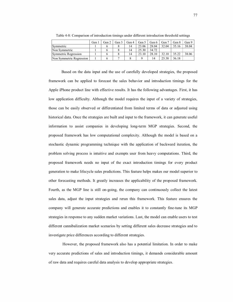
77
Table 4-8: Comparison of introduction timings under different introduction threshold settings
Gen 1 Gen 2 Gen 3 Gen 4 Gen 5 Gen 6 Gen 7 Gen 8 Gen 9 Symmetric 1 6 8 14 23.06 28.04 32.04 35.16 38.04 Non Symmetric 1 6 8 14 25.30 34.72 Symmetric Regression 1 6 8 14 23.10 28.10 32.10 35.22 38.06 Non Symmetric Regression 1 6 7 8 9 14 25.38 36.18
Based on the data input and the use of carefully developed strategies, the proposed
framework can be applied to forecast the sales behavior and introduction timings for the
Apple iPhone product line with effective results. It has the following advantages. First, it has
low application difficulty. Although the model requires the input of a variety of strategies,
those can be easily observed or differentiated from limited terms of data or adjusted using
historical data. Once the strategies are built and input to the framework, it can generate useful
information to assist companies in developing long-term MGP strategies. Second, the
proposed framework has low computational complexity. Although the model is based on a
stochastic dynamic programming technique with the application of backward iteration, the
problem solving process is intuitive and exempts user from heavy computations. Third, the
proposed framework needs no input of the exact introduction timings for every product
generation to make lifecycle sales predictions. This feature helps makes our model superior to
other forecasting methods. It greatly increases the applicability of the proposed framework.
Fourth, as the MGP line is still on-going, the company can continuously collect the latest
sales data, adjust the input strategies and rerun this framework. This feature ensures the
company will generate accurate predictions and enables it to constantly fine-tune its MGP
strategies in response to any sudden market variations. Last, the model can enable users to test
different cannibalization market scenarios by setting different sales decrease strategies and to
investigate price differences according to different strategies.
However, the proposed framework also has a potential limitation. In order to make
very accurate predictions of sales and introduction timings, it demands considerable amount
of raw data and requires careful data analysis to develop appropriate strategies.

78
In the next section, we apply the cannibalization model to forecast a brand new MGP
line based on sales data from an existing product line. As an illustrative case study, we use
Apple’s iPhone product line to predict its iPad product line.
4.3 Case Study III: Forecasting a Brand New Multiple-Generation Product Line
In this section, we attempt to predict a new MGP line according to the market
information acquired from an on-going MGP line. The process of applying the
cannibalization model to forecast a new product line is slightly different from that for an
existing product line. When predicting a new product line mapping by using the sales from an
existing and on-going product line, we need to perform an additional technological analysis
on the major specifications of the two product lines. The reason for verifying technological
similarity at the beginning is to ensure the lines have high similarity in technological
capabilities and product type so that it is feasible to use sales data from one to predict results
for the other. Next we introduce a quantitative approach to verify technological similarity
between MGP lines.
4.3.1 Technological Similarity Examination
The first stage of this case study involves verifying the technological similarity
between the new MGP line and the reference existing product line. We propose an approach
based on the concept of the function sharing matrix from Kalyanasundaram and Lewis (2011),
which also incorporates a new rating system to verify functional similarity between product
lines. Kalyanasundaram and Lewis analyzed product function structures and relative function
flows involved with the two objective products, and then they introduced a function sharing
matrix that decomposed the studied products into three segments: 1) the principal flow chunk,
2) the variant flow chunk, and (3) the auxiliary chunk. In this study, we do not investigate the
product structures of the two objective products but instead focus on the functions. Therefore,
we adopt the concept of the function sharing matrix and introduce a technological similarity

79
matrix (TSM). In the TSM, we distinguish the technologies involved in a product line
according to the three suggested categories: 1) principal, 2) variant, and 3) auxiliary
technologies. To simplify the use of TSM and to increase the numbers of product lines for
comparison at a time, we eliminate the pair-wise comparison feature and directly compare the
technological similarity from the reference MGP line to the new and other product lines. It
should be noted that the technologies we compare across different product lines are only the
core technologies that remain unchanged within each product line. Of additional note, the
reason we compare the reference product line to the new product line is that we assume that
the new product line has more novel technologies than the existing one; accordingly, to
identify the technological similarity we need only to consider the existing prevalent
technologies. Table 4-9 illustrates the TSM used in this study.
We classified the major technologies of the iPhone product line into three
technological groups, and the result is shown in Table 4-9. Because the iPhone is a smart
phone product line, the key elements of basic cell phone operations are categorized as the
principal technologies. Lesser critical elements are grouped into the variant technologies, and
the remainders are considered the auxiliary technologies. To quantitatively distinguish the
technological similarity, we propose a simple way to calculate the technological similarity
index. To minimize the subjectivity in judgment ratings, we use a three-level scoring system.
If the target technology is exactly the same between any product line and the reference
product line, we assign a score of 2. If the target technology is similar (perform similar tasks)
but not exactly the same, a score of 1 is given. Furthermore, if the target technology is totally
different from the product line, then a score of 0 is assigned. After evaluating all the
technologies, we sum up the scores for each product line and divide by the overall score of
the reference product line, which is 2 times the number of technologies. The existing
reference product line will have the highest technological similarity index, which is 1. The
higher the score in the index, the more similar the two product lines are. Note that in this case
study, we consider all three technological groups to have equal importance.
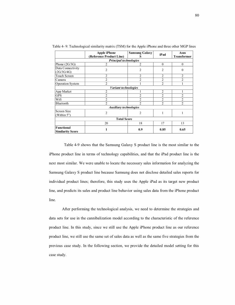
80
Table 4- 9: Technological similarity matrix (TSM) for the Apple iPhone and three other MGP lines
Apple iPhone (Reference Product Line)
Samsung Galaxy S iPad Asus
Transformer Principal technologies
Phone (2G/3G) 2 2 0 0 Data Connectivity (2G/3G/4G) 2 2 2 0
Touch Screen 2 2 2 2 Camera 2 2 2 2 Operation System 2 1 2 1
Variant technologies App Market 2 1 2 1 GPS 2 2 2 2 Wifi 2 2 2 2 Bluetooth 2 2 2 2
Auxiliary technologies Screen Size (Within 5") 2 2 1 1
Total Score 20 18 17 13
Functional Similarity Score 1 0.9 0.85 0.65
Table 4-9 shows that the Samsung Galaxy S product line is the most similar to the
iPhone product line in terms of technology capabilities, and that the iPad product line is the
next most similar. We were unable to locate the necessary sales information for analyzing the
Samsung Galaxy S product line because Samsung does not disclose detailed sales reports for
individual product lines; therefore, this study uses the Apple iPad as its target new product
line, and predicts its sales and product line behavior using sales data from the iPhone product
line.
After performing the technological analysis, we need to determine the strategies and
data sets for use in the cannibalization model according to the characteristic of the reference
product line. In this study, since we still use the Apple iPhone product line as our reference
product line, we still use the same set of sales data as well as the same five strategies from the
previous case study. In the following section, we provide the detailed model setting for this
case study.

81
4.3.2 Model Setting
In this section, we address our implementation of the proposed framework to forecast
Apple Inc.’s popular MGP line, the Apple iPads, using the sales data of its successful product
line, the Apple iPhones. Similar to the previous case study, we use the same four strategies
from the sales increase scenario and only the convergence strategy from the sales decrease
strategy in the cannibalization model. Furthermore, in this current study, we use the same 17
terms of sales data from the Apple iPhones with adjustments to forecast the Apple iPad
product line.
To create the dynamic state model for this case study, we started by introducing the
basic model parameters. First we defined the unit of time t and the total lifecycle duration, T.
We considered one accounting quarter as a basic time unit. Since we had no information for
the planned lifecycle duration of the Apple iPad product line, we ran six different lifecycle
durations (T = 30, 35, 40, 45, 50 and 55) to determine the differences in lifecycle predictions.
In addition, different from the previous case study, we used 150 states in the model, where
each state represents 500,000 units of sales.
Next, we need to determine the value settings for the five strategies. Since we did not
know the original demand forecast for the iPad product line, we used a simple way to
determine a scale difference between the two product lines. We used the real first seven
periods of sales of iPads (from 2010 Q2 to 2012 Q1 for comparison with the real first seven
terms of sales for iPhones (from 2007 Q4 to 2009 Q1), and found the total sales of iPad
product lines to be 3.18 times of the iPhone product line. Given this ratio, we re-scaled the
parameters setting from those we applied in the previous section. Table 4-10 shows the
settings for all three strategies (conservative increase, oscillation increase and successive
product generation introduction), where the unit is the state. The successive product
generation introduction strategy is more complicated than the others, and Table 4-10 reveals
only the potential sales variations when applying this strategy. For the successive product
generation introduction strategy, we needed to consider two critical parameters: the

82
introduction threshold function (Th(t)) and the expected profit gain (EP). The former, Th(t), is
a symmetric function. We chose all the preceding time periods as observation points, and set
the mildest slope between the sales volume of the latest observation point to all the other
points at Th(t). The detailed slope and intercept values for Th(t) are shown in Table 4-11. We
defined EP simply as the sales increment rate between the total sales in the time period where
a successive product generation is introduced to the market over the total sales in the previous
quarter. We connected all the EP ratios we observed from the data in Table 4-3 in Section 4-2,
and we assumed EP to be linear and to vary with time.
Two strategies not included in Table 4-10 are the aggressive strategy and the
convergence strategy. For the convergence strategy, we set the converge rate (D3) = 0.8, the
convergence threshold (Cg) as state 9.6, and the rapid convergence rate as (Cv) = 7.08 states.
For the aggressive strategy, we used the time and sales differences between the first and
fourth generations of iPhones at the introduction for each time period to generate the slope
and intercept for t ≤ (T+1)/2, and we used symmetric settings for t > (T+1)/2. The detailed
slopes and intercepts of the aggressive strategy are shown in Table 4-11. In addition, we
assumed costs in the cannibalization model to be due only to sales increase strategies. We set
the cost of using the successive product generation introduction strategy to be 10 states of
product sales amount, and we set state 1 for the other three strategies.
Table 4-10: Settings for three sales increase strategies
Strategy Parameter Increase Rate Probability B1 14.23 0.625 Conservative Increase Strategy B2 9.44 0.375 C1 1.27 0.200 Oscillation Increase Strategy C2 -7.47 0.800 I1 -7.94 0.500 Successive Product Generation Introduction Strategy I2 -14.39 0.500

83
Table 4-11: Parameter settings for the three time-dependent symmetric functions
For t ≦ (1+t)/2 For t ≧ (1+t)/2 Function Slope Intercept Slope Intercept
Agg(t) 4.01 -2.29 -4.01 4.01 * (t+1) - 2.29 Th(t) 2.67 9.06 -2.67 2.68 * (t+1) - 2.67
The total expected future sales K(x) needed to be given to solve the cannibalization
model. We assumed the iPhone product line sells 100 states of units per time period. We
further supposed that the sales variance would be 20%. T is the total lifecycle duration, x
indicates the state, and unit profit margin is U. Thus, K(x) will be:
TUxTUxUT
UTxK
33.333,133000,000,40 ]150/)22.0(000,500100[
8.0000,500100)(
(Eq. 4-18)
After defining the model settings, strategies and boundaries, we ran the
cannibalization model and then the Monte Carlo forward iteration using the same Excel-VBA
based program in Appendix C. The cannibalization model yielded two strategy maps from
both sales scenarios. Figure 4-5 is the strategy map derived from the sales increase scenario
data. In Figure 4-5, the x-axis is time and y-axis is state, and each color represents a sales
increase strategy to be applied at a certain time and state. Figure 4-5 shows the simulated
lifecycles at T = 35 for the iPad product line.
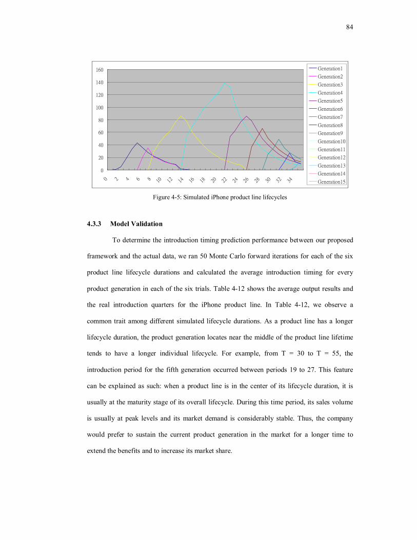
84
0
20
40
60
80
100
120
140
160
0 2 4 6 8 10 12 14 16 18 20 22 24 26 28 30 32 34
Generation1
Generation2
Generation3
Generation4
Generation5
Generation6
Generation7
Generation8
Generation9
Generation10
Generation11
Generation12
Generation13
Generation14
Generation15
Figure 4-5: Simulated iPhone product line lifecycles
4.3.3 Model Validation
To determine the introduction timing prediction performance between our proposed
framework and the actual data, we ran 50 Monte Carlo forward iterations for each of the six
product line lifecycle durations and calculated the average introduction timing for every
product generation in each of the six trials. Table 4-12 shows the average output results and
the real introduction quarters for the iPhone product line. In Table 4-12, we observe a
common trait among different simulated lifecycle durations. As a product line has a longer
lifecycle duration, the product generation locates near the middle of the product line lifetime
tends to have a longer individual lifecycle. For example, from T = 30 to T = 55, the
introduction period for the fifth generation occurred between periods 19 to 27. This feature
can be explained as such: when a product line is in the center of its lifecycle duration, it is
usually at the maturity stage of its overall lifecycle. During this time period, its sales volume
is usually at peak levels and its market demand is considerably stable. Thus, the company
would prefer to sustain the current product generation in the market for a longer time to
extend the benefits and to increase its market share.

85
Table 4-12: Six sets of average successive product generation introduction timings from six different product line lifecycle durations comparing to the actual Apple iPhone MGP line
iPad Gen 1 Gen 2 Gen 3 Gen 4 Gen 5 Gen 6 Gen 7 Gen 8 Gen 9 Gen 10 T = 30 1 6 8 14 19.12 23.1 26.1 28.38 T = 35 1 6 8 14 21.2 25.58 28.88 31.88 33.9 T = 40 1 6 8 14 23.26 28.24 32.24 35.38 38.1 T = 45 1 6 8 14 25.12 30.62 34.94 38.6 41.6 43.86 T = 50 1 6 8 14 27.08 33.16 38.12 42.12 45.22 48.08 Actual 1 4 8
The proposed framework used in this study is capable of applying the observed 17
terms of sales data from the Apple iPhone product line with appropriate adjustments to
forecast the sales behavior and introduction timings for the Apple iPad MGP line, which is a
product line with high functional similarity. As noted previously, the proposed framework has
four distinct advantages; it has low application difficulty, it has low computational complexity,
the introduction timing for every product generation is automatically predicted from the
proposed framework and need not be given, and it forecasts a new product line using sales
data from an existing product line, allowing companies to construct future product and market
strategies for the product line well in advance. Moreover, when the product line has been
introduced and is active in the market, the company can apply the proposed framework to
directly forecast more accurate future sales performance and potential product line behavior
for the entire product line. And, as noted earlier, the model can enable users to prepare for
market cannibalization situations in advance by setting different cannibalization scenarios
into sales decrease strategies, helping users test different pricing strategies under different
market situations.
The proposed framework does carry a potential challenge. To make very accurate
predictions of sales and introduction timings, it demands considerable raw data and requires
careful data analysis to develop appropriate strategies.
In the next section, the technology evolution model is introduced.

86
4.4 Technology Evolution Model
We start by formulating the basic technology evolution model, which embeds the
technology evolution concern into the cannibalization model and considers only a single
technology evolving over time. In this model, in addition to using state variable X(t) to
records the sales status, we introduce a new state variable Y(t) to record the change of the
technology substitution status during the lifecycle of the MGP line.
To begin with, we first define the expected profit function Fi(x, y, t) as:
Fi(x, y, t) = maximum expected profit between time period t and the expected end of
life of the MGP line for sales scenario i, given that X(t) = x and Y(t) = Y.
(Eq. 4-19)
In this model, there are two cases for i since we consider two different sales scenarios
(increase or decrease). These are F1(x, y, t) and F2(x, y, t), each representing the optimal profit
of the sales increase scenario and sales decrease scenario when product sale is in state x and
technology evolution status is in state y in time period t. The actual optimal profit of the entire
product line Fi(x, y, T) is acquired by summation of all the expected profits at the last time
period.
After defining Fi(x, y, t), we need to clarify the expected profit values corresponding
to the strategy chosen at state x and y, and time period t, preceding time period T. Let,
Vj(x, y, t) = the optimal profit when strategy j is selected for time period t from time
period t+1 onward, given that X(t) = x and Y(t) = y.
(Eq. 4-20)
Forming strategies corresponding to potential sales behaviors is the next step after the
model definition. In this model, we adopt the same six strategies and two sales scenarios from

87
the cannibalization model.. The sales increase scenario aims at the sales variation for the
target product generation in the period between its market debut and the introduction of its
successor. It offers a choice of the four strategies analyzed previously: aggressive increase,
conservative increase, oscillation increase, and successive product generation introduction.
The sales decrease scenario aims at the sales situation when a target product generation
gradually decays toward the end of its life. Likewise, it offers two strategies: decrease and
convergence. The settings of the seven strategies used in this technology evolution model are
somewhat different from those in the cannibalization model. Below, we introduce the
strategies of the two scenarios, respectively.
Table 4-13: Technology evolution model parameters
Th(t) Threshold for introducing the successive generation of product at time period t. Unit is state.
Agg(t) Product sales when applying aggressive increase strategy at time period t. Unit is state. PCon Probability for profit increase when applying the conservative strategy. Poscr Probability for profit increase or decrease when applying the oscillation strategy. PIntro Probability for profit decrease when applying the successive product generation
introduction strategy. PCv Probability for the rapid sales converge when applying the converge strategy. B1 The more profit increment when applying the conservative strategy. Unit is state. B2 The less profit increment when applying the conservative strategy. Unit is state. C1 The more profit increment or the less profit decrement when applying the oscillation
strategy. Unit is state. C2 The more profit decrement when applying the oscillation strategy. Unit is state. I1 The less profit decrement when applying the successive product generation introduction
strategy. Unit is state. I2 The more profit decrement when applying the successive product generation introduction
strategy. Unit is state. EP Expected profit gain under the strategy if introducing the successive generation of product. D1 Rate of the more profit decrement when applying the decrease strategy. Unit is state. D2 Rate of the less profit increment when applying the decrease strategy. Unit is state. D3 Constant decrease rate of the oscillation decrease strategy. Unit is state.
CAgg Cost involved when adopting the aggressive increase strategy. Unit is state. CCon Cost involved when adopting the conservative increase strategy. Unit is state. Cosc Cost involved when adopting the oscillation strategy. Unit is state. CDecr Cost involved when adopting the decreasing strategy. Unit is state. CCv Cost involved when adopting the converge strategy. Unit is state.
CIntro Costs involved in introducing the successive generation of product. Unit is state. T Entire (multiple-generation) product life span. Unit is season.
X(t) Amount of profit at the start of time period t. Unit is state. Cg Convergence threshold for the sales decrease scenario. Unit is state. Cv The rapid sales convergence in the converge strategy. Unit is state. xcrit The critical level for product sales in sales increase model. Unit is state. ycrit The critical level for product sales in sale decrease model. Unit is state.

88
Y(t) Technology substitution status at the start of time period t. Unit is state. E(t) Actual technology substitution status at the start of time period t. Unit is state.
Ad(t) Adjusted technology substitution status at the start of time period t. Unit is state. TE Technology evolution threshold. Unit is state. EA The early adoption threshold for new generation of technology. Unit is state. CA The catch-up adoption threshold for new generation of technology. Unit is state. FA The enforced adoption threshold for new generation of technology. Unit is state. DA Delayed adoption threshold. Unit is state. k The unit of the technology substitution rate per time period. Unit is state.
4.4.1 Sales Increase Scenarios
In this section, we provide further explanation about the four sales increase strategies.
1. The Aggressive Increase Strategy
Otherwise 0
1 x if)()1(1
tAggxtX
ktYtAd )()1(
Else
TEE(t) If )()1(
CrityktE
tE
)]1(),1(min[)1(1 tEtAdtY
(Eq. 4-21)
The aggressive strategy only takes place at the time period when a product generation
enters the market. In this model, for the sales status X(t), we still define State 1 as the critical

89
state, and the successive product generation ready to be introduced to the market must wait at
the critical state. When the debut decision is made, the successive product generation follows
the aggressive strategy and jumps to the corresponding state. Therefore, the aggressive
increase strategy only occurs when a new generation of the product is at State 1. The
introduction sales performance of a new product generation should vary with time and the
stage of the product line lifecycle. To better fit the real world conditions, we define the sales
performance of the aggressive increase strategy into a polynomial function Agg(t), which
varies with time t and is symmetric with respect to (T+1)/2. In addition, the aggressive
increase strategy cannot be selected when a product generation is no longer at state 1. As for
the technology substitution status Y(t+1) at time t+1, we consider two conditions, E(t+1) and
Ad(t+1). E(t+1) is the actual technology substitution status at time t+1, and it has a critical
threshold TE, which is the technology evolution threshold. If E(t+1) stands above TE, it
means the next generation of technology evolves and could be applied to products. Once the
new technology is available, E(t+1) returns to the critical level and moves to represent the
substitution status of the new technology. Meanwhile, Ad(t+1) indicates the adjusted
technology substitution status at time t+1. The reason we use two different variables is that
E(t+1) reveals only the actual technology substitution status of the market; accordingly, we
use Ad(t+1) to record the generations of technologies adopted by the products. Note that we
assume the rate of technology substitution is linear in this study; thus, both E(t+1) and Ad(t+1)
grow linearly with a constant rate k. For Y(t+1), we select the lower value from E(t+1) and
Ad(t+1). Equation 4-22 presents the stochastic dynamic programming formulation of the
optimal profit when selecting the aggressive strategy:
Otherwise 0
1 If C-1) t,)]1(),1'(min[,)1((),,( Agg
1
xtEtAdtAggxFtyxV
(Eq. 4-22)

90
2. The Conservative Increase Strategy
1 xIf ,
)P-(1y probabilit with
Py probabilit with )1(
Con2
Con12 Bx
BxtX
Where B1 > B2
ktYtAd )()1(
Else
TEE(t) If )()1(
CrityktE
tE
)]1(),1(min[)1(2 tEtAdtY
(Eq. 4-23)
Equation 4-23 indicates the two possible conditions when selecting the conservative
strategy. For sales state X(t+1), if the current state of a product generation is not at State 1,
product sales may increase from their current state to a much higher state B1 with a
probability, PCon, or to a slightly higher state with a probability, (1 - PCon). In addition, the
technology substitution status for the next time period is selected from the lower value
between the adjusted and the actual technology substitution status elements. Equation 4-24
provides the optimal profit when selecting the conservative strategy in the stochastic dynamic
programming form. This strategy is not considered if the technology substitution status stands
between the enforced adoption threshold FA and the delayed adoption threshold DA. The
reasoning is that if it falls between FA and DA, it means that the current technology is widely
prevalent but that the company does not have a product incorporating this generation of
technology. Thus, the company must release a new product generation with this mainstream
technology to catch up with its competitors and to maintain its market position.

91
Otherwise 0
DA y and 1 x )1)],1(),1'(min[,()1( ORFA y and 1 xIf )1)],1(),1'(min[,(
),,( 2
1
2 ConCon
Con
CttEtAdBxFPttEtAdBxFP
tyxV
(Eq. 4-24)
3. The Oscillation Increase Strategy
1 xIf ,
)P-(1y probabilit with Py probabilit with
)1(Osc2
Osc13 Cx
CxtX
Where C1 > C2
ktYtAd )()1(
Else
TEE(t) If )()1(
CrityktE
tE
)]1(),1(min[)1(3 tEtAdtY
(Eq. 4-25)
When selecting the oscillation increase strategy, sales may slightly increase or
decrease in the amount of C1 with a probability POsc , or drop moderately in the amount of C2
with a probability, (1 - PDecr). It is noted that C1 may be positive or negative, but C2 is
negative. Moreover, the technology substitution status for the next time period is still chosen
from the lower value between the adjusted technology substitution status and the actual
technology substitution status. Equation 4-26 is the stochastic dynamic programming
formulation for optimal profit under the oscillation increase strategy.

92
As with the conservative increase strategy, the oscillation increase strategy is not
taken into account if the technology substitution status stands between the enforced adoption
threshold FA and delayed adoption threshold DA.
OtherwiseCttEtAdCxFP
ttEtAdCxFPtyxV OscOsc
Osc
0DA y and 1 x )1)],1(),1'(min[,()1(
ORFA y and 1 xIf )1)],1(),1'(min[,(),,( 2
1
3
(Eq. 4-26)
In addition, for each time period t, product sales are constrained between a set of
boundaries xcrit and the highest state. xcrit is the critical level of product sales, and any product
generation with a state smaller or equal to xcrit which is State 1, is considered to be withdrawn
from the market. Similarly, technology substitution status is bounded between the critical
state ycrit and the highest state at each time period t. ycrit is the critical state of technology
substitution status, and it is defined to be State 1. Every time a new technology emerges or
when a new generation of product is equipped with the latest technology, the technology
substitution status returns to the critical state ycrit.
4. The Successive Product Generation Introduction Strategy
The company may decide to introduce the successive product generation rather than
applying any of the possible strategies if the current product sales exceed the introduction
threshold Th(t). In this model, we consider that threshold should be dynamic and follow a
polynomial function that varies with time and is symmetric at t = (T+1)/2. As with our prior
example, introducing the successive generation may incur introduction costs, or, it may yield
the highest gain in return as future profit. Additionally, as previously, since our model
incorporates cannibalization, sales for the target product generation do not fall to the critical
state but drop to a pair of lower states and follow a set of stochastic probabilities when a
successive generation of product is introduced to the market. Equation 4-27 shows that when

93
the current product sales level exceeds the product introduction threshold Th(t); product sales
may drop I1 state with a probability of Pintro, or decrease I2 state with a probability of (1 –
pintro).
The technology substitution status for this strategy varies with different conditions, of
which there are five. First, if the technology substitution status is less than the early adoption
threshold EA, the company can only introduce the successive product generation with existing
technology. Second, if the technology substitution status stands upon the early adoption
threshold EA but beneath the catch-up adoption threshold CA, the company can choose to
release the successive generation of product with either the existing technology or the newly
mature technology. We use a pair of probabilities PNew and (1-PNew) to represent the chance of
implementing the new or extant technology in the successive product generation respectively.
Third, if the technology substitution status stands above the catch-up adoption threshold CA
but below the enforced adoption threshold FA, the company has to implement the latest
available technology when releasing the competitive successive generation of product in order
to catch up with the market leaders. Fourth, if the technology substitution status is higher than
the enforced adoption threshold FA but lower than the delayed adoption threshold DA, all the
other sales increase strategies are exclusive at this time and the company must release the
successive product generation with the extant mature and prevalent technology. For the last
condition, if the technology substitution status is higher than the delayed adoption threshold
DA, then the company would consider bypassing the current generation of technology and
delay the introduction of the successive product generation until the next generation of
technology is available. Equation 4-28 is the stochastic dynamic programming function for
the optimal profit under the successive product generation introduction strategy. In Equation
4-28, EP is the expected profit gain when introducing the successive generation of the product.
On the other hand, if current product sales are within the threshold, then the company should
not decide to introduce the successive generation of the product since doing this would not
benefit the company in the long run but may significantly harm its profitability.

94
)( tThxIf ,
)P-(1y probabilit with
Py probabilit with )1(
Intro2
Intro14 Ix
IxtX
Where 0 > I1 > I2
EAyIf
ktYtAd )()1(
Else
TEE(t) If )()1(
CrityktE
tE
)]1(),1(min[)1(4 tEtAdtY
CAyEAIf
If the new generation of technology is not adopted,
ktYtAd )()1(
Else
TEE(t) If )()1(
CrityktE
tE
)P-(1y probabilit with )]1(),1(min[)1( New4 tEtAdtY
If the new generation of technology is adopted,
CritytAd )1(

95
Else
TEE(t) If )()1(
CrityktE
tE
Py probabilit with )1( New4 CritytY
FAyCAIf
CritytAd )1(
Else
TEE(t) If )()1(
CrityktE
tE
CritytY )1(4
DAyFAIf
CritytAd )1(
Else
TEE(t) If )()1(
CrityktE
tE
CritytY )1(4
DAyIf
ktYtAd )()1(
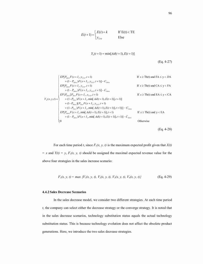
96
Else
TEE(t) If )()1(
CrityktE
tE
)]1(),1(min[)1(4 tEtAdtY
(Eq. 4-27)
Otherwise 0 )]1)],1(),1(min[,()1(
EAy and Th(t) If )1)],1(),1(min[,([ )]}1)],1(),1(min[,()-(1
)1,,()[-1( )]1)],1(),1(min[,()-(1
CAyEA and Th(t) If )1,,([{ )]1,,()1(
FAyCA and Th(t) If )1,,([)]1,,()1(
AyFA and Th(t) If )1,,([
),,(
2
1
2
2
1
1
2
1
2
1
4
IntroIntro
Intro
IntroNew
CrilNewIntro
New
CrilNewIntro
IntroCrilIntro
CrilIntro
IntroCrilIntro
CritIntro
CttEtAdIxFPxttEtAdIxFPEP
CttEtAdIxFPtyIxFPP
ttEtAdIxFPxtyIxFPPEP
CtyIxFPxtyIxFPEP
CtyIxFPDxtyIxFPEP
tyxV
(Eq. 4-28)
For each time period t, since F1(x, y, t) is the maximum expected profit given that X(t)
= x and Y(t) = y, F1(x, y, t) should be assigned the maximal expected revenue value for the
above four strategies in the sales increase scenario:
F1(x, y, t) = max {V1(x, y, t), V2(x, y, t), V3(x, y, t), V4(x, y, t)} (Eq. 4-29)
4.4.2 Sales Decrease Scenarios
In the sales decrease model, we consider two different strategies. At each time period
t, the company can select either the decrease strategy or the converge strategy. It is noted that
in the sales decrease scenarios, technology substitution status equals the actual technology
substitution status. This is because technology evolution does not affect the obsolete product
generations. Here, we introduce the two sales decrease strategies.

97
1. The Decrease Strategy
CgxIf ,
)P-(1y probabilit with
Py probabilit with )1(
Dec2
Dec15 Dx
DxtX
Where 0 > D1 > D2
Else
TEE(t) If )()1(
CrityktE
tE
)1()1(5 tEtY
(Eq. 4-30)
In the decrease strategy, if the current state of the target product generation exceeds
the convergence threshold Cg, then the sales may drop either slightly by D1 state or
significantly by D2, each with a probability of PDec or (1 – PDec). Equation 4-31 presents the
stochastic dynamic programming formulation of the optimal profit when choosing the
decrease strategy:
Otherwise 0)1),1(,()1(
Cg(t) xIf )1),1(,(),,( 2
1
5 DecDec
Dec
CttEDxFPttEDxFP
tyxV
(Eq. 4-31)
2. The Convergence Strategy
CgxIf ,
)()1( 36 txDtX
Otherwise

98
)P-(1y probabilit with Py probabilit with )(
)1(Cv
Cv36 Cvx
txDtX
Else
TEE(t) If )()1(
CrityktE
tE
)1()1(6 tEtY
(Eq. 4-32)
In this study, we define “convergence” as the condition when product sales gradually
move toward “zero”, where the target product generation is about to be removed from the
market. We consider that convergence includes two scenarios. For the first scenario, when the
product sales stand above the convergence threshold Cb, they slowly converge. We assume
that the product sales no longer drop by constant states but diminish following a certain
discount rate. For the second scenario, when the current state is equal or lower than the
converge threshold Cb, the product sales drop in two different ways. In this scenario, the
product sales may rapidly converge by Cv states with a probability of PCon, or may still drop
following the same discount rate with a probability of (1-PCon). This scenario represents the
situation when a product generation is close to its end of life, and the company may retain it
in the market for a while or may directly withdraw it. When the current state of a product
generation is lower than the critical state, it is removed from the market. Equation 4-33
provides the optimal profit when selecting the convergence strategy in the stochastic dynamic
programming form.
CgxIf ,
Cg xIf C- )1),1(),((),,( Cv36 ttEtxDFtyxV

99
Otherwise
1 CvxIf
Cv36 C- )1),1(),(()1()1),1(,)((),,( ttEtxDFPttECvtxFPtyxV ConCon
(Eq. 4-33)
For each time period t, since F2(x, y, t) is the maximum expected profit given that X(t)
= x and Y(t) = y, F2(x, y, t) should be assigned the maximal expected revenue values for the
above two strategies in the sales decrease scenario:
F2(x, y, t) = max {V5(x, y, t), V6(x, y, t)} (Eq. 4-34)
After formulating this model, backward iteration is used to solve it. When applying
the backward iteration, we start from the last term t = T and move backward in time. Thus, the
end condition Fi(x,y,T), which is the total expected future profits for the product line, must be
given. We assume Fi(x, y, T) is a function K(x), and we define it in the case study section.
The technology evolution model also outputs the two optimal time-state strategy
maps for both scenarios, indicating the optimal strategy the company should apply for a
targeted product generation at each time and state under either of the two sales scenarios. The
strategy maps allow the company to develop long-term product line strategies or to adjust its
strategies toward dynamic market changes.
In the next section, we demonstrate a case study applying the technology evolution
model to the Apple iPhone product line.
4.5 Case Study IV: Technology Evolution Model

100
In this section, we again take Apple’s iPhone product line as our target to demonstrate
the technology evolution model. In this study, we still use the 17 periods of observed data to
forecast the sales behavior and successive product generation introduction timings for the
entire iPhone product line. In addition, we use 150 states in the model, where each state
represents 200,000 units of sales, and T = 50.
In the technology evolution model, the most critical element is how to model the
technology substitution status. There are two main problems when formulating the evolution
of technology. First, the assessment of the market status for a certain technology may be
troublesome because the acquisition of data is very difficult. Second, technology may not
evolve linearly.
After searching through the literature, we figured out ways to tackle the above two
problems. To acquire macroscopic data for the cell phone market, we located research from
Kim (2009), who surveyed 1074 cell phone models from major manufacturers (including
Nokia, Motorola, Sony-Ericsson, Samsung and LG, whose combined market share from 2002
to 2008 ranges from 74.5% to 81%) and analyzed the relationships between several
specifications and market shares for each manufacturers. We adopted Kim’s cell phone
market survey data and tried to abstract the usable market trend information to use in the
technology evolution model. In order to demonstrate the technology evolution model, we
needed to select one technology as our target to monitor its evolution. In this case study, we
chose mobile network generation as our objective technology. Mobile network is the kernel of
cell phones, and it also confines the development of cell phones. The first generation (1G)
mobile network was introduced to the market in 1979. In March 2011, LTE Advanced was
formally selected as the standard for the fourth generation (4G) mobile network, and is
expected to be operational globally in 2013. Between the development of 1G and 4G, the
network download speed evolved from 29 kbyte/s to 1gbyte/s (1 million kbyte/s). The
dramatic growth of network transmission speed pushed mobile phone manufacturers to
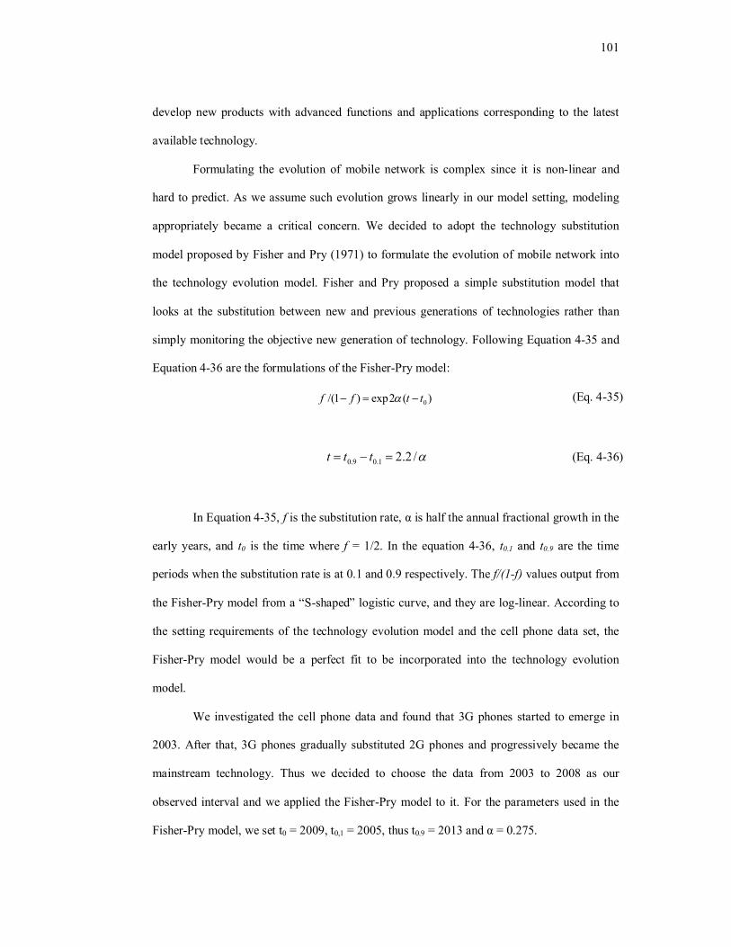
101
develop new products with advanced functions and applications corresponding to the latest
available technology.
Formulating the evolution of mobile network is complex since it is non-linear and
hard to predict. As we assume such evolution grows linearly in our model setting, modeling
appropriately became a critical concern. We decided to adopt the technology substitution
model proposed by Fisher and Pry (1971) to formulate the evolution of mobile network into
the technology evolution model. Fisher and Pry proposed a simple substitution model that
looks at the substitution between new and previous generations of technologies rather than
simply monitoring the objective new generation of technology. Following Equation 4-35 and
Equation 4-36 are the formulations of the Fisher-Pry model:
)(2exp)1/( 0ttff (Eq. 4-35)
/2.21.09.0 ttt (Eq. 4-36)
In Equation 4-35, f is the substitution rate, α is half the annual fractional growth in the
early years, and t0 is the time where f = 1/2. In the equation 4-36, t0.1 and t0.9 are the time
periods when the substitution rate is at 0.1 and 0.9 respectively. The f/(1-f) values output from
the Fisher-Pry model from a “S-shaped” logistic curve, and they are log-linear. According to
the setting requirements of the technology evolution model and the cell phone data set, the
Fisher-Pry model would be a perfect fit to be incorporated into the technology evolution
model.
We investigated the cell phone data and found that 3G phones started to emerge in
2003. After that, 3G phones gradually substituted 2G phones and progressively became the
mainstream technology. Thus we decided to choose the data from 2003 to 2008 as our
observed interval and we applied the Fisher-Pry model to it. For the parameters used in the
Fisher-Pry model, we set t0 = 2009, t0,1 = 2005, thus t0.9 = 2013 and α = 0.275.

102
Table 4-14 shows the numbers of cell phones released by the major manufacturers
between 2003 and 2008 with 2G/3G mobile network capabilities. Table 4-15 is the
comparison of the f/(1-f) values between the real data and the outputs from the Fisher-Pry
model, where the row “Real f/(1-f)” indicates the real data and the row “Projected f/(1-f)” is
the calculation output from the Fisher-Pry model.
Table 4- 14: The numbers of cell phones with 2G/3G mobile network capabilities from 2003 to 2008
2003 2004 2005 2006 2007 2008 2G Phones 101 122 215 188 218 183 3G Phones 1 6 28 51 86 71
Table 4- 15: The comparison of f/(1-f) between the real data and the outputs from the Fisher-Pry model
2003 2004 2005 2006 2007 2008 2009 2010 2011 2012 2013 Real f/(1-f) 0.01 0.0517 0.1497 0.3723 0.6515 0.633 Projected f/(1-f) 0.0369 0.0639 0.1108 0.192 0.3329 0.5769 1 1.733 3.004 5.207 9.0250
However, to use this data in the technology evolution model, there is one more
problem. In the technology model, the unit of time is an accounting season, but in Table 4-15
the unit of time is a year. We used an easy way to assess the seasonal f/(1-f) values. Using
year 2005 as an example, we set the first to fourth season each as 2004.25, 2004.5, 2004.75
and 2005, respectively. Since f/(1-f) values depict a logistic curve, log f/(1-f) values form a
straight line. A technology can have a market portion from 0 to 100%; the f/(1-f) values
mostly fall between 0.01 to 100. Thus, the main body of the log f/(1-f) line will stand between
-2 and 2. As log f/(1-f) is a linear function, we can assess the seasonal unit of the technology
substitution rate k from log f/(1-f) and k = 0.0597. In this case study, we adjust log f/(1-f)
values and set them into the E(t). We add 2 to all the log f/(1-f ) values and define E(t) to
range between 0 and 4. In addition, since we have k = 0.0597 and E(t) ranges from 0 to 4, we
separate Y(t) into 67 states and each state is k. When a new technology is available, E(t) drops
to the critical state yCri, which is 0. Besides, as we know the 4G will become available in 2013,
we set the log f/(1-f) from 2012 as the technology evolution threshold (TE) and TE is at State
46.

103
For the constraints of Y(t), we try to use different combinations of constraints to see if
there is any effect to the introduction timings products and the adoption of new technology.
For the basic setting, we set EA is f = 0.1, CA is f = 0.3, EA is f = 0.5, DA is f =0.7. Also, we
try two variable settings. We fix CA and set EA to reflect six different situations from f = 0.35
to f = 0.65, and fix EA and set CA to be in a set of different conditions from f = 0.15 to 0.45.
The strategy settings in the technology evolution model remain the same as those in
the cannibalization model. Table 4-16 shows the settings for three strategies where the unit is
one state. The successive product generation introduction strategy is more complicated, and
Table 4-16 reveals only the potential sales variations when applying this strategy. The two
additional parameters for the successive product generation introduction strategy are the
introduction threshold function (Th(t)), and the expected profit gain (EP). The introduction
threshold function, Th(t), is a symmetric function as well as the sales function for the
aggressive increase strategy Agg(t). For the aggressive strategy, we use the time and sales
differences between the first and the fourth generations of iPhones at the each of its
introduction time period to generate the slope and intercept. The detailed slope and intercept
values for Th(t) and Agg(t) are shown in Table 4-17. As for the EP, we simply define it as the
sales increment rate between the total sales in the time period where a successive product
generation is introduced to the market over the total sales in the previous quarter. We connect
all the EP ratios we observed from iPhone’s sales, and assume EP is linear and varies with
time as well.
As for the convergence strategy, we set the converge rate as (D3) = 0.8, the convergence
threshold (Cg) as state 7.54, and the rapid convergence rate (Cv) = 5.56 states. In addition, we
assume costs only involve the sales increase strategies. We set the cost of using the successive
product generation introduction strategy to be 10 states of product sales amount and 1 state
for the rest of the three strategies.
Table 4- 16: Settings for three of the strategies

104
Strategy Parameter Increase Rate Probability B1 11.19 0.625 Conservative Increase Strategy B2 7.42 0.375 C1 1.00 0.200 Oscillation Increase Strategy C2 -5.87 0.800 I1 -6.24 0.500 Successive Product Generation Introduction Strategy I2 -11.31 0.500
Table 4- 17: Parameter settings for the three time-dependent symmetric functions
For t ≦(1+t)/2 For t ≧(1+t)/2 Function Slope Intercept Slope Intercept Agg(t) 3.15 -1.80 -3.15 127.37 Th(t) 2.10 7.13 -2.10 93.29
The total expected future sales K(x) needs to be given in order to solve the
cannibalization model. We assume the iPhone product line sells 100 states of units per time
period. We further suppose that the sales variance would be 20%. T is the total lifecycle
duration, x indicates the state, and unit profit margin is U. Thus, K(x) will be:
TUxTUxUT
UTxK
33.333,53000,000,16 ]150/)22.0(000,200100[
8.0000,200100)(
(4-37)
After defining all the model settings, strategies and boundaries used in this case study,
we need to solve this technology evolution model. We apply the backward iteration to solve
DSVMs from both the sales increase and sales decrease scenario. After the backward iteration,
we receive the optimal strategic maps from both sales scenarios. For the next step, we apply
the Monte-Carlo forward iteration to obtain the potential lifetime prediction of the iPhone
product line. We developed an Excel-VBA based software to do the computation for the
model, and the code is provided in Appendix D. Figure 4-6 is a set of prediction output from
the Monte-Carlo forward iteration. Table 4-18 is the introduction timings for the iPhone
product line with different EA and CA setting. In Table 4-18, the real introduction timings for
the real iPhone product line is also included. We can see that the model predictions are very
different from reality, the reason is that in this illustrative case study we choose to use a much
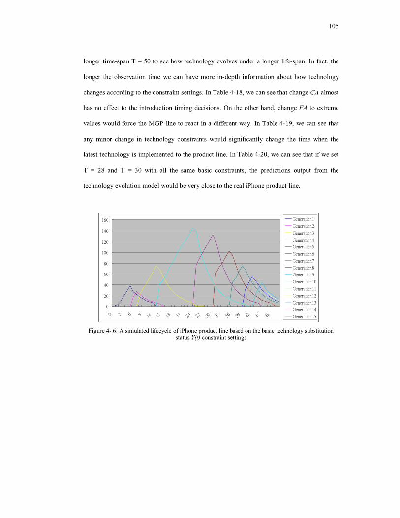
105
longer time-span T = 50 to see how technology evolves under a longer life-span. In fact, the
longer the observation time we can have more in-depth information about how technology
changes according to the constraint settings. In Table 4-18, we can see that change CA almost
has no effect to the introduction timing decisions. On the other hand, change FA to extreme
values would force the MGP line to react in a different way. In Table 4-19, we can see that
any minor change in technology constraints would significantly change the time when the
latest technology is implemented to the product line. In Table 4-20, we can see that if we set
T = 28 and T = 30 with all the same basic constraints, the predictions output from the
technology evolution model would be very close to the real iPhone product line.
0
20
40
60
80
100
120
140
160
0 3 6 9 12 15 18 21 24 27 30 33 36 39 42 45 48
Generation1
Generation2
Generation3
Generation4
Generation5
Generation6
Generation7
Generation8
Generation9
Generation10
Generation11
Generation12
Generation13
Generation14
Generation15
Figure 4- 6: A simulated lifecycle of iPhone product line based on the basic technology substitution status Y(t) constraint settings

106
Table 4- 18: Introduction timings comparison with the real iPhone product line with different FA and CA settings
Gen 1 Gen 2 Gen 3 Gen 4 Gen 5 Gen 6 Gen 7 Gen 8 Gen 9 Gen 10
Gen 11
Gen 12
FA = 35% 1 2 6 8 14 25.16 31.74 36.74 41.04 44.62 47.62 49.08 FA = 40% 1 5 7 9 14 25.24 31.74 36.74 40.84 44.52 47.52 49.64 FA = 45% 1 6 8 14 25.18 31.76 36.8 40.92 44.5 47.48 49.52 FA = 50% 1 6 8 14 25.34 31.76 36.84 40.92 44.56 47.56 49.66 FA = 55% 1 6 8 14 25.2 31.78 36.84 40.96 44.52 47.52 49.69 FA = 60% 1 6 8 14 25.26 31.72 36.78 40.84 44.48 47.46 49.58 FA = 65% 1 6 8 14 25.2 31.8 36.88 41.04 44.54 47.52 49.68
Real iPhone 1 6 10 14 19 22 CA = 15% 1 6 8 14 25.24 31.86 36.9 40.98 44.46 47.42 49.57 CA = 20% 1 6 8 14 25.26 31.84 36.88 40.94 44.6 47.6 49.74 CA = 25% 1 6 8 14 25.42 31.9 36.96 41.04 44.64 47.62 49.8 CA = 30% 1 6 8 14 25.34 31.76 36.84 40.92 44.56 47.56 49.66 CA = 35% 1 6 8 14 25.24 31.74 36.74 40.84 44.42 47.42 49.56 CA = 40% 1 6 8 14 25.14 31.64 36.78 41 44.54 47.52 49.67 CA = 45%' 1 6 8 14 25.36 31.86 36.92 41.08 44.5 47.48 49.68
Table 4- 19: The timings that the target technology is adopted by the product line
3G 4G FA = 35% 2 46.36 FA = 40% 5 41.06 FA = 45% 6 38.58 FA = 50% 6 40.98 FA = 55% 6 43.14 FA = 60% 6 38.64 FA = 65% 6 41.3 CA = 15% 6 47.3 CA = 20% 6 49.7 CA = 25% 6 41.34 CA = 30% 6 40.98 CA = 35% 6 46.46 CA = 40% 6 40.94 CA = 45%' 7.08 38.46
Table 4- 20: Comparison between shorter life-span T settings with the real iPhone data
Gen 1 Gen 2 Gen 3 Gen 4 Gen 5 Gen 6 Gen 7 Gen 8 Real iPhone 1 6 10 14 19 22
T = 28 1 6 8 14 18.82 22.44 25.44 27.54 T = 30 1 6 8 14 19.12 23.1 26.1 28.4

Chapter 5
Conclusion and Future Work
In this chapter, we provide the conclusion as well as the future research directions for this
research.
5.1 Conclusion
In this work, we propose a new framework to support the analysis of MGP lines. In the
proposed framework, we apply a DSVM to formulate the lifetime behaviors of MGP lines. The
proposed framework considers two substitution scenarios between consecutive product
generations. In the first scenario, the successor fully substitutes the market position of the current
product generation. In the second scenario, multiple generations of products directly compete
with each other in the same market. In this study, several real-world case studies are provided to
validate our proposed frameworks. A case involving IBM mainframe computer systems is
adopted to demonstrate the basic model, and the on-going sales data of Apple iPhones is analyzed
to verify different applications of the cannibalization model.
In addition, we bring the concern of technology evolution into the proposed framework.
For most MGP lines, especially for technology products, one or more technologies involved in
the product line evolve over time. The status of technology evolution may cause companies to
rethink their market strategies, especially product introduction decisions. Thus, companies should
continuously monitor the latest available technologies in the market to ensure they adopt the
correct strategies. In this study, we look into the situation where one single technology evolves
over time in a MGP line from both substitution scenarios.

108
The proposed framework centers on a DSVM. This model outputs a set of time-state
strategy maps for the target product line. In the next stage, Monte Carlo forward iteration is
adopted to simulate a complete lifecycle of the product line. When properly analyzing raw sales
data and transforming it into well defined strategies, the proposed framework can generate a close
lifetime prediction for the target MGP line.
The proposed framework has four major contributions. First, it has real market data
applicability. Real market scenarios can be analyzed using proper strategies under the proposed
framework. Second, it can automatically generate key measures. With the input of properly set
strategies, the proposed framework can automatically output the best time-state strategies,
introduction timings, and potential lifetime behaviors for every product generation within a MGP
line. Third, it has low applicability difficulty for companies to implement. Companies can easily
model their current market environment with the proposed framework. Since companies possess
more detailed and accurate market data and knowledge to input, the proposed framework can
return credible forecasting performance. Fourth, the proposed framework provides a virtual
environment for companies to verify potential market strategies in advance prior to directly
implementing them in the market. In addition, the proposed framework can assist companies in
developing more flexible market strategies toward the dynamic market environment through the
lifecycle of MGP lines. With the strategy maps output from the DSVM, companies are able to fit
their current market status to the relative state and adopt the optimal strategy to ensure
profitability.
5.2 Limitations of the Research
The proposed framework also has limitations. First, to acquire highly accurate predictions,
it requires the input of very precise and adequate market and operational data to properly deduce
accurate strategies from product sales trends. Second, for forecasting the behaviors of an on-

109
going product line, the longer the observation time span, the more accurate the predictions. Third,
for forecasting a new product line, close predictions can only mirror a highly similar product line.
Fourth, the proposed framework generates forecasts based on the past sales trend. Thus, if the
market has unexpected shifts (e.g., the emergence of breakthrough technology), the proposed
framework is not able to reflect those changes. Fifth, the proposed framework has difficulty with
modeling a market scenario involving interactions among multiple competitors.
5.3 Future Research Direction
In our future work, we will focus on three directions. First, we will incorporate the concern
of multiple-technology evolutions into the existing framework. In this study, we investigated a
situation in which only a single technology evolves over the lifecycle of a MGP lines. However,
most of the real-world MGP lines involve more than one evolving technology. As multiple
evolving technologies involve in a product line, their interactions and priorities need to be taken
into concern. Second, we will look at how cannibalization can affect the sales and profits of MGP
lines. Simulation-based techniques are a potential approach to combine with our proposed
framework in order to examine different strategies for preventing cannibalization. Third, various
strategy settings will be examined. We will formulate actual market traits into strategies so that
the proposed framework can generate more realistic and valuable decisions for companies. For
instance, we will test strategies with different marketing considerations, investigate the price
differences, etc.
Moreover, we will consolidate the proposed framework by validating several constraint and
threshold settings. Unverified assumptions will also be validated with additional sensitivity
analyses.

References
Arslan H, Kachani S, Shmatov K. 2007. Optimal Product Introduction and Life Cycle Pricing
Policies for Multiple Product Generations under Competition. Journal of Revenue
and Pricing Management 8(5): 438-451.
Bardhan AK , Chanda U. 2008. A Model for First and Substitution Adoption of Successive
Generations of A Product. International Journal of Modeling and Simulation 8(4):
487-494.
Bryan A, Ko J, Hu,S J, Koren Y. 2007. Co-evolution of product families and assembly
systems. CIRP Annals-Manufacturing Technology 56(1): 41-44.
Clark CW. 1993. Dynamic Models of Behavior: An extension of life history theory. Tree 8(6):
205-209.
Clark CW, Mangel M. 2000. Dynamic State Variable Models in Ecology – Methods and
Applications. Oxford University Press, New York. 304 p.
Dacko S G, Liu BS, Sudharshan D, Furrer O. 2008. Dynamic Capabilities to Match Multiple
Product Generations and Market Rhythm. European Journal of Innovation
Management 11(4): 441-471.
Deltas G , Zacharias E. 2006. Entry Order and Pricing over the Product Cycle: The Transition
from the 486 to the Pentium Processor. International Journal of Industrial
Organization 24: 1041-1069.
Edelheit LS. 2004. Perspective on GE Research & Development. Research Technology
Management 47(1): 49-55.
Erhun F, Concalves P, Hopman J. 2007. The Art of Managing New Product Transitions. MIT
Sloan Management Review 48(3): 72-80.

111
Fenton A ,Rands SA (2004). Optimal Parasite Infection Strategies: A state-dependent
approach. International Journal for Parasitology 34: 813-821.
Fisher J C, Pry RH. 1971. A Simple Substitution Model of Technological Change.
Technological Forecasting and Social Change 3: 75-88.
Gaonkar R S, Viswanadham N. 20055. Strategic Sourcing and Collaborative Planning in
Internet-Enabled Supply Chain Networks Producing Multiple-generation Products.
IEEE Transactions on Automation Science and Engineering (1): 54-66.
Hill K. 1993. Life History Theory and Evolutionary Anthropology. Evolutionary
Anthropology (3): 78-88.
Houston A, Clark C, McNamara J, Mangel M. 1988. Dynamic Models in Behavioural and
Evolutionary Ecology. Nature 332(3): 29-34.
Huang CY, Tzeng GH. 2008. Multiple Generation Product Life Cycle Predictions Using a
Novel Two-stage Fuzzy Piecewise Regression Analysis Method. Technology
Forecasting & Social Change 75: 12-31.
Ishigami Y, Yagi H, Kondoh S, Umeda Y, Shimomura Y, Yoshioka M. 2003. Development of
a Design Methodology for Upgradability Involving Changes of Functions.
Proceedings of the 3rd International Symposium on EcoDesign: Environmentally
Conscious Design and Inverse Manufacturing; 2003 December; Tokyo, Japan: IEEE
Cat No 03EX895003.
Kalyanasundaram V, Lewis K. 2011. A Function Based Approach for Product Integration.
Proceedings of the ASME 2011 International Design Engineering Technical
Conferences & Computers and Information in Engineering Conference; 2011 August;
Washington DC: IDETC2011-47922, 17 p.
Kim, TH. 2009. An Investigation on the Importance of Design Form and Function: Market
success and consumer preferences [dissertation]. [University Park, (PA)]:

112
Pennsylvania State University.
Ko J, Hu SJ. 2009. Manufacturing System Design Considering Stochastic Product Evolution
and Task Recurrence. [Internet.] [cited in Journal of Manufacturing Science and
Engineering 131(5). Available from: http://dx.doi.org/10.1115/1.4000095
Krankel RM, Duenyas I, Kapuscinski R. 2006. Timing Successive Product Introductions with
Demand Diffusion and Stochastic Technology Improvement. Manufacturing and
Service Operations Management 8(2): 119-135.
Lande R. 1982. A Quantitative Genetic Theory of Life History Evolution. Ecology 63(2): 607-
615.
Li Y, Xue D, Gu P. 2008. Design for product adaptability. Concurrent Engineering Research
and Applications16(3): 221-232.
Li Z, Gao L. 2008. The Effects of Sharing Upstream Information on Product Rollover.
Production and Operations Management 17(5): 522-531.
Lim WS, Tang CS. 2006. Optimal Product Rollover Strategies. European Journal of
Operational Research 174: 905-922.
Lippitz MJ. 1999. Examination of Optimal Upgrade Timing and Best Value: DoD acquisition
of commercial vs. military custom flat panel displays. Proceedings of SPIE 3690 - The
International Society for Optical Engineering; 1999 August; Orlando, FL; 154-163.
Liu H, Özer Ö. 2009. Managing A Product Family under Stochastic Technological
Changes. International Journal of Production Economics 122: 567-580.
Mahajan V, Muller E. 1996. Timing, Diffusion, and Substitution of Successive Generation of
Technological Innovations: The IBM Mainframe Case. Technological Forecasting
and Social Change 51: 109-132.
Marchetti C. 1987. Infrastructures for Movement. Technological Forecasting and Social
Change 32: 373-393.
113
McAdams DA, Stone RB, Wood KL. 1999. Functional Interdependance and Product
Similarity Based on Customer Needs. Research in Engineering Design 11: 1-19.
McAdams DA,Wood KL 2002. A Quantitative Similarity Metric for Design-by-Analogy.
Journal of Mechanical Design 124: 173-182.
McNamara JM, Houston AI. 1996. State-dependent Life Histories. Nature 380: 215-221.
Modis T. 2007. Strength and Weakness of S-curves. Technological Forecasting and Social
Change 74: 866-872.
Morgan LO, Morgan RM, Moore WL. 2001. Quality and Time-to-Market Trade-offs When
There Are Multiple Product Generations. Manufacturing and Service Operations
Management 3(2): 89-104.
Nakicenovic N. 1979. Software Package for the Logistic Substitution Model, RR-79-12.
Research report [Internet.] [International Institute for Applied Systems Analysis;
1979; Laxenburg, Austria.] Available from:
http://www.iiasa.ac.at/publication/more_RR-79-012.php
Norto JA, Bass FM. 1987. A Diffusion Theory Model of Adoption and Substitution for
Successive Generations of High-Technology Products. Management Science 33(9):
1069-1086.
Orbach Y, Fruchter GE. 2011.Forecasting Sales and Product Evolution: The case of the
hybrid/electric car. Technological Forecasting and Social Change 78: 1210-1226.
Ofek E, Sarvary M. 2003. R&D, Marketing, and the Success of Next-Generation Products.
Marketing Science 2(3): 355-370.
Purcell J, Brodin A. 2007. Factors Influencing Route Choice by Avian Migrants: A dynamic
programming model of Pacific brant migration. Journal of Theoretical Biology 49:
804-816.
Rogers CM, Smith JNM. 1993. Life-History Theory in the Nonbreeding Period: Trade-offs in

114
avian fat reserves?” Ecology 74(2): 419-426.
Rogers EM. 1995. Diffusion of innovation, 4th ed. Simon and Schuster, New York. 518 p.
Sääkjärvi M, Lampinen M. 2005.Consumer Perceived Risk in Successive Product Generations.
European Journal of Innovation Management 8(2): 145-156.
Sherrat TN, Speed MP, Ruxton GD. 2004. Natural Selection on Unpalatable Species Imposed
by State-dependent Foraging Behaviour. Journal of Theoretical Biology 28: 217-226.
Thietart RA, Vivas R. 1984. An Empirical Investigation of Success Strategies for Businesses
along the Product Life Cycle. Management Science 30(12): 1405-1423.
Umeda Y, Ishii M, Yoshioka M, Shimomura Y, Tomiyama T. 1996. Supporting Conceptual
Design Based on the Function-behavior-state modeler. Artificial Intelligence for
Engineering Design, Analysis and Manufacturing. AIEDAM 10(4): 275-288.
Umemori Y, Kondoh S, Umeda, Y, Shimomura Y, and Yoshioka M. 2001. Design for
Upgradable Products Considering Future Uncertainty. In: Proceedings of the 2nd
International Symposium on EcoDesign: Environmentally Conscious Design and
Inverse Manufacturing; 2001 December; Tokyo, Japan.
Wikipedia File: IPhone sales per quarter [Internet]. MySchizoBuddy, Here to Help; June 2009;
quarterly. Accessed November 2012. Available from:
http://en.wikipedia.org/wiki/File:IPhone_sales_per_quarter_simple.svg
Xing K, Belusko M, Luong L, Abhary K. 2007 An Evaluation Model of Product
Upgradeability for Remanufacture. International Journal of Advanced Manufacturing
Technology 35(1-2): 1-14.
Yang CL, Ni MH, Wei CC. 2011.Timing for Launching a New Product to Maximize Overall
Profit. Concurrent Engineering: Research and Applications 19(3): 201-212.

Appendix A
VBA Code of the Program “Multiple-Generation Product Line Simulator”
Sub simulator()
Dim a1 As Double
Dim a2 As Double
Dim d1 As Double
Dim d2 As Double
Dim c1 As Double
Dim c2 As Double
Dim up As Double
Dim paii As Double
Dim pcii As Double
Dim pd As Double
Dim t As Double
Dim h As Double
Dim il As Double
Dim ciagg As Double
Dim cd As Double
Dim cicon As Double
Dim xp1 As Double
Dim xpp1 As Double
Dim xp2 As Double

116
Dim xpp2 As Double
Dim xp3 As Double
Dim xpp3 As Double
Dim xp4 As Double
Dim state(30, 2, 100) As Double
Dim com(1, 2) As Double
Dim f(30, 100) As Double
Dim det As Double
Load UserForm1
Load UserForm2
UserForm1.Show
t = UserForm2.TextBox1.Value
a1 = UserForm2.TextBox12.Value
a2 = UserForm2.TextBox13.Value
d1 = UserForm2.TextBox14.Value
d2 = UserForm2.TextBox15.Value
c1 = UserForm2.TextBox18.Value
c2 = UserForm2.TextBox19.Value
up = UserForm2.TextBox16.Value
ciagg = UserForm2.TextBox24.Value
cicon = UserForm2.TextBox25.Value
cd = UserForm2.TextBox27.Value

117
h = UserForm2.TextBox31.Value
paii = UserForm2.TextBox33.Value
pcii = UserForm2.TextBox34.Value
il = UserForm2.TextBox35.Value
pd = UserForm2.TextBox36.Value
det = UserForm2.TextBox37.Value
Sheets("sheet1").Select
Cells(1, 1) = "State"
Cells(1, 2) = "Agg Increase"
Cells(1, 3) = "Con Increase"
Cells(1, 4) = "Decrease"
Cells(1, 5) = "Intro New"
For i = 1 To 30
f(i, t) = 463 * (1 + ((i - 17) / 30) ^ 3)
Next
For i = 1 To t - 1
For j = 1 To 30
Cells(j + 1, 1) = j
xp1 = j + a1 - ciagg
xpp1 = j + a2 - ciagg

118
If xpp1 >= 1 And xp1 <= 30 Then
Cells(j, 2) = paii * f(xp1, t - i + 1) + (1 - paii) * f(xpp1, t - i + 1)
Else
Cells(j, 2) = 0
End If
xp2 = j + c1 - cicon
xpp2 = j + c2 - cicon
If xpp2 >= 1 And xp2 <= 30 Then
Cells(j, 3) = pcii * f(xp2, t - i + 1) + (1 - pcii) * f(xpp2, t - i + 1)
Else
Cells(j, 3) = 0
End If
xp3 = j - d1 - cd
xpp3 = j - d2 - cd
If xpp3 >= 1 And xp3 <= 30 Then
Cells(j, 4) = pd * f(xp3, t - i + 1) + (1 - pd) * f(xpp3, t - i + 1)
Else
Cells(j, 4) = 0
End If
If j >= h Then
xp4 = il
Cells(j, 5) = up + f(xp4, t - i + 1) - det

119
Else
Cells(j, 5) = 0
End If
com(1, 1) = 0
com(1, 2) = 0
For k = 1 To 4
If com(1, 1) < Cells(j, k + 1) Then
com(1, 1) = Cells(j, k + 1)
com(1, 2) = k
End If
Next
state(j, 1, t - i) = com(1, 1)
state(j, 2, t - i) = com(1, 2)
f(j, t - i) = com(1, 1)
Next j
Next i
For i = 1 To t - 1
Cells(1, i + 1) = i
For j = 1 To 30
Cells(j + 1, 1) = j
Cells(j + 1, i + 1) = state(j, 2, i)

120
Next
Next
MsgBox "The optimal expected profit is " & state(il, 1, 1)
End Sub

121
Appendix B
VBA Code of the Program “Monte Carlo Forward Iteration Simulator”
Sub Monte_carlo()
Dim os(24) As Double
Dim r As Double
For k = 1 To 50
Sheets("sheet1").Select
os(1) = 1
r = Rnd()
If r > 0.5 Then
os(2) = 1 + 7
Else
os(2) = 1 + 1
End If
For i = 2 To 23
Select Case Cells(os(i), i)
Case 1
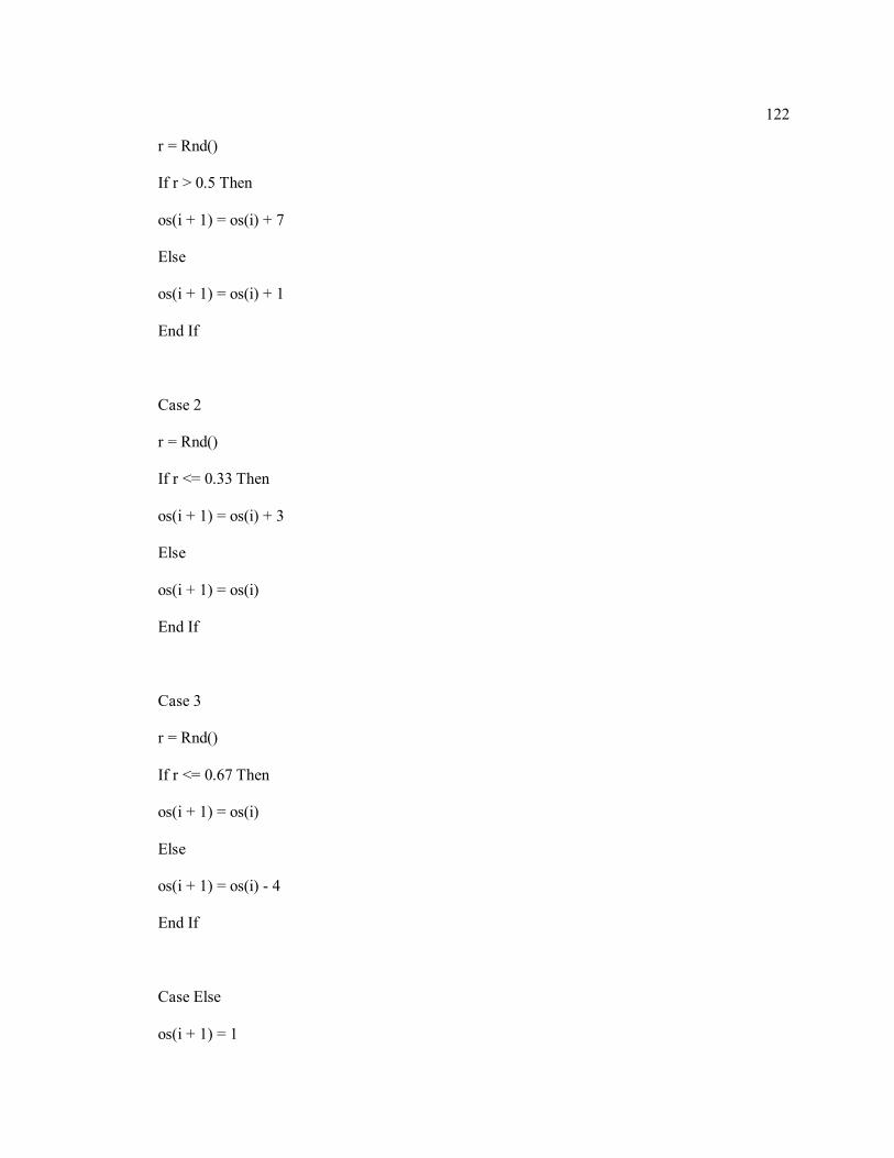
122
r = Rnd()
If r > 0.5 Then
os(i + 1) = os(i) + 7
Else
os(i + 1) = os(i) + 1
End If
Case 2
r = Rnd()
If r <= 0.33 Then
os(i + 1) = os(i) + 3
Else
os(i + 1) = os(i)
End If
Case 3
r = Rnd()
If r <= 0.67 Then
os(i + 1) = os(i)
Else
os(i + 1) = os(i) - 4
End If
Case Else
os(i + 1) = 1

123
End Select
Next i
Sheets("sheet2").Select
For i = 1 To 24
Cells(1, i + 1) = i
Cells(k + 1, i + 1) = os(i)
Next i
Next k
Cells(1, 1) = "Time"
Cells(2, 1) = "Optimal State"
End Sub

124
Appendix C
VBA Code of the Cannibalization Model with the Monte Carlo Forward Iteration
Sub new_model()
Dim icon1 As Double
Dim icon2 As Double
Dim iagg1 As Double
Dim iosc1 As Double
Dim iosc2 As Double
Dim intro1 As Double
Dim intro2 As Double
Dim intro1p As Double
Dim intro2p As Double
Dim it1 As Double
Dim it2 As Double
Dim pi1 As Double
Dim pi2 As Double
Dim pi3 As Double
Dim pi4 As Double
Dim ex As Double
Dim ci1 As Double
Dim ci2 As Double
Dim ci3 As Double
Dim ci4 As Double

125
Dim exc As Double
Dim dec1 As Double
Dim dec2 As Double
Dim dcon As Double
Dim conth As Double
Dim pd1 As Double
Dim pd2 As Double
Dim pd3 As Double
Dim cd1 As Double
Dim cd2 As Double
Dim in1 As Double
Dim in3 As Double
Dim in2(200, 100) As Double
Dim a1i As Double
Dim a2i As Double
Dim x(1, 2) As Double
Dim y(1, 2) As Double
Dim z(200) As Double
Dim inc(200, 100, 10) As Double
Dim dec(200, 100, 10) As Double

126
Dim a1(200) As Double
Dim a2(200) As Double
Dim s1(200, 100, 2) As Double
Dim s2(200, 100, 2) As Double
Dim s3(200, 100) As Integer
Dim s4(200, 100, 10, 2) As Double
Dim counter(10, 1) As Integer
Dim counter2(1, 2) As Double
Dim state As Integer
Dim t As Integer
Dim gn(200, 100, 2) As Double
Dim ste(200, 100, 2) As Double
Dim r As Double
Dim th(100) As Double
Dim z0 As Double
Dim z1 As Double
Dim z2 As Double
Dim mi1 As Double
Dim mi2 As Double
Dim mi3 As Double

127
Dim mi4 As Double
Dim ct As Double
Dim cin As Double
Dim ma1 As Double
Dim ma2 As Double
Dim ma3 As Double
Dim ma4 As Double
Dim u1 As Double
Dim u2 As Double
Dim u3 As Double
Dim u4 As Double
Dim minc As Double
Dim maxc As Double
Dim iy(50, 20) As Integer
Dim tp As Double
Dim run As Integer
Dim av As Double
Dim emp As Integer
'=====================finish variables declaration=========================
'=====================Variable value assignment==========================
'--------------System parameters-----------------------------
t = 40
state = 150
'-------------Increase stragegy------------------------------

128
icon1 = 7.42
icon2 = 11.19
iosc1 = -5.87
iosc2 = 1
it1 = -11.31
it2 = -6.24
'-------------Cost for increase strategy--------------------
ci1 = 200
ci2 = 200
ci3 = 200
ci4 = 2000
'------------------------------------------------------------
'--------------Probability for increase strategy-------------
pi2 = 0.375
pi3 = 0.8
pi4 = 0.5
'============================================================
'-------------Decrease stragegy------------------------------
'dec1 =
'dec2 =
dcon = -5.5644
conth = 7.5438
pd3 = 0.8
'------------------------------------------------------------
'-------------Cost for decrease stragegy---------------------

129
cd1 = 0
cd2 = 0
'------------------------------------------------------------
'--------------Probability for decrease strategy-------------
'pd1 =
pd2 = 0.5
'============================================================
'--------------Constraints-----------------------------------
'============================================================
'Slopes for Aggressive strategy
ma1 = 3.1505 * 200000
ma2 = -1.8 * 200000
ma3 = -ma1
ma4 = ma1 * (t + 1) + ma2
'------------------------------------------
'Slopes for Introduction threshold function
mi1 = 2.1015 * 200000
'mi1 = 771549.8
mi2 = 7.1261 * 200000
'mi2 = -3140649
mi3 = -mi1
mi4 = mi1 * (t + 1) + mi2
'------------------------------------------
'Slopes for Upper bound function

130
u1 = 5.3687 * 200000
u2 = 2.2377 * 200000
u3 = -u1
u4 = u1 * (t + 1) + u2
'============================================================
'Forward iteration runs
run = 50
'============================================================
'Expected overall profits
a1i = 100 * t * 200000
a2i = a1i * 0.2 * 2 / state
For i = 1 To state
a1(i) = a1i * 0.8 + i * a2i
s1(i, t, 1) = a1(i)
s2(i, t, 1) = a1(i)
Next
'==============finsih variable values assignmen==============
'==============Dynamic State Variable starts===========================
For i = 1 To t - 1
For j = 1 To state
'===============================================================
'Increase
'------------Aggressive Increase---------------------------------------

131
If (t - i) <= (t + 1) / 2 Then
iagg1 = (ma1 * (t - i) + ma2) / 200000
Else
iagg1 = (ma3 * (t - i) + ma4) / 200000
End If
If iagg1 >= state Then
iagg1 = state
End If
If iagg1 < 0 Then
iagg1 = 0
End If
If j = 1 Then
z1 = s1(Int(j + iagg1), t + 1 - i, 1) * (1 - (j + iagg1 - Int(j + iagg1)))
z2 = s1(Int(j + iagg1 + 1), t + 1 - i, 1) * (j + iagg1 - Int(j + iagg1))
inc(j, t - i, 1) = z1 + z2 - ci1
s4(j, t - i, 1, 1) = inc(j, t - i, 1)
s4(j, t - i, 1, 2) = 1
inc(j, t - i, 2) = 0
inc(j, t - i, 3) = 0
inc(j, t - i, 4) = 0
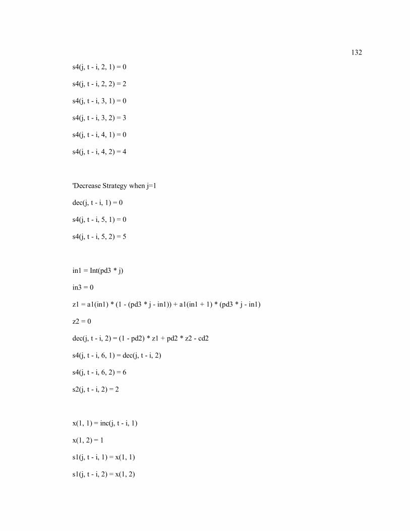
132
s4(j, t - i, 2, 1) = 0
s4(j, t - i, 2, 2) = 2
s4(j, t - i, 3, 1) = 0
s4(j, t - i, 3, 2) = 3
s4(j, t - i, 4, 1) = 0
s4(j, t - i, 4, 2) = 4
'Decrease Strategy when j=1
dec(j, t - i, 1) = 0
s4(j, t - i, 5, 1) = 0
s4(j, t - i, 5, 2) = 5
in1 = Int(pd3 * j)
in3 = 0
z1 = a1(in1) * (1 - (pd3 * j - in1)) + a1(in1 + 1) * (pd3 * j - in1)
z2 = 0
dec(j, t - i, 2) = (1 - pd2) * z1 + pd2 * z2 - cd2
s4(j, t - i, 6, 1) = dec(j, t - i, 2)
s4(j, t - i, 6, 2) = 6
s2(j, t - i, 2) = 2
x(1, 1) = inc(j, t - i, 1)
x(1, 2) = 1
s1(j, t - i, 1) = x(1, 1)
s1(j, t - i, 2) = x(1, 2)

133
Else 'j<>1
inc(j, t - i, 1) = 0
s4(j, t - i, 1, 1) = 0
s4(j, t - i, 1, 2) = 1
'------------Conservative Increase-------------------------------------
If (t - i) <= (t / 2) Then
ub = (u1 * (t - i) + u2) '/ 200000
Else
ub = (u3 * (t - i) + u4) '/ 200000
End If
If j <= ub Then
If j + icon1 <= state Then
z1 = pi2 * (s1(Int(j + icon1), t + 1 - i, 1) * (1 - (j + icon1 - Int(j + icon1))) + s1(Int(j + icon1 + 1),
t + 1 - i, 1) * (j + icon1 - Int(j + icon1)))
If j + icon2 <= state Then
z2 = (1 - pi2) * (s1(Int(j + icon2), t + 1 - i, 1) * (1 - (j + icon2 - Int(j + icon2))) + s1(Int(j + icon2
+ 1), t + 1 - i, 1) * (j + icon2 - Int(j + icon2)))
Else
z2 = 0

134
End If
inc(j, t - i, 2) = z1 + z2 - ci2 * j * 0.05
s4(j, t - i, 2, 1) = z1 + z2 - ci2 * j * 0.05
s4(j, t - i, 2, 2) = 2
Else
z1 = 0
If j + icon2 <= state Then
z2 = (1 - pi2) * (s1(Int(j + icon2), t + 1 - i, 1) * (1 - (j + icon2 - Int(j + icon2))) + s1(Int(j + icon2
+ 1), t + 1 - i, 1) * (j + icon2 - Int(j + icon2)))
Else
z2 = 0
End If
End If
If z1 + z2 >= ci2 Then
inc(j, t - i, 2) = z1 + z2 - ci2
s4(j, t - i, 2, 1) = z1 + z2 - ci2
s4(j, t - i, 2, 2) = 2
Else
s4(j, t - i, 2, 1) = 0
s4(j, t - i, 2, 2) = 2
End If
Else
inc(j, t - i, 2) = 0

135
s4(j, t - i, 2, 1) = 0
s4(j, t - i, 2, 2) = 2
End If
'-------------Increase Oscillation--------------------------------------
If j + iosc1 >= 1 Then
z1 = pi3 * (s1(Int(j + iosc1), t + 1 - i, 1) * (1 - (j + iosc1 - Int(j + iosc1))) + s1(Int(j + iosc1 + 1), t
+ 1 - i, 1) * (j + iosc1 - Int(j + iosc1)))
If j + iosc2 <= state Then
z2 = (1 - pi3) * (s1(Int(j + iosc2), t + 1 - i, 1) * (1 - (j + iosc2 - Int(j + iosc2))) + s1(Int(j + iosc2 +
1), t + 1 - i, 1) * (j + iosc2 - Int(j + iosc2)))
Else
z2 = (1 - pi3) * s1(state, t + 1 - i, 1)
End If
inc(j, t - i, 3) = z1 + z2 - ci3
s4(j, t - i, 3, 1) = z1 + z2 - ci3
s4(j, t - i, 3, 2) = 3
Else
inc(j, t - i, 3) = 0
s4(j, t - i, 3, 1) = 0
s4(j, t - i, 3, 2) = 3
End If

136
'-----------Intro Strategy-----------------------------------------------
If (t - i) < (t + 1) / 2 Then
th(t - i) = (mi1 * (t - i) + mi2) / 200000
Else
th(t - i) = (mi3 * (t - i) + mi4) / 200000
End If
If j + it1 > state Then
intro1p = state
Else
intro1p = j + it1
End If
If j + it2 > state Then
intro2p = state
Else
intro2p = j + it2
End If
If th(t - i) > 0 Then
If j >= th(t - i) And j + it1 >= 1 Then

137
If intro1p >= 1 Then
If intro1p < state Then
z1 = pi4 * (s1(Int(intro1p), t + 1 - i, 1) * (1 - (intro1p - Int(intro1p))) + s1(Int(intro1p + 1), t + 1 -
i, 1) * (intro1p - Int(intro1p)))
Else
z1 = pi4 * s1(state, t + 1 - i, 1)
End If
Else
z1 = 0
End If
If intro2p >= 1 Then
If intro2p < state Then
z2 = (1 - pi4) * (s1(Int(intro2p), t + 1 - i, 1) * (1 - (intro2p - Int(intro2p))) + s1(Int(intro2p + 1), t
+ 1 - i, 1) * (intro2p - Int(intro2p)))
Else
z2 = (1 - pi4) * s1(state, t + 1 - i, 1)
End If
Else
z2 = 0
End If
z0 = (z1 + z2)
tp = t - i
'-----------------------------------

138
If tp < 5 Then 't-i<5
inc(j, t - i, 4) = (z0) * (t - i) * 0.749177 - ci4
s4(j, t - i, 4, 1) = inc(j, t - i, 4) '
s4(j, t - i, 4, 2) = 4
Else
If tp <= 9 Then '5<=t-i<9
inc(j, t - i, 4) = (z0) * ((-2.0487324) * (t - i) + 19.853146) - ci4 'single
s4(j, t - i, 4, 1) = inc(j, t - i, 4)
s4(j, t - i, 4, 2) = 4
Else
If tp <= 13 Then '9<=t-i<13
inc(j, t - i, 4) = (z0) * (0.066164 * (t - i) + 0.819081) - ci4 'single'
s4(j, t - i, 4, 1) = inc(j, t - i, 4)
s4(j, t - i, 4, 2) = 4
Else 't-i>=13
inc(j, t - i, 4) = (z0) * 1.6792 - ci4 'single
s4(j, t - i, 4, 1) = inc(j, t - i, 4)
s4(j, t - i, 4, 2) = 4
End If

139
End If
End If
'------------------------------------
Else
inc(j, t - i, 4) = 0
s4(j, t - i, 4, 1) = 0
s4(j, t - i, 4, 2) = 4
End If
Else
inc(j, t - i, 4) = 0
s4(j, t - i, 4, 1) = 0
s4(j, t - i, 4, 2) = 4
End If
'-----------Decrease Strategy--------------------------------------------
dec(j, t - i, 1) = 0
s4(j, t - i, 5, 1) = 0
s4(j, t - i, 5, 2) = 5
'-----------Converge Strategy--------------------------------------------

140
If j > conth Then
in1 = Int(pd3 * j)
dec(j, t - i, 2) = s1(in1, t + 1 - i, 1) * (1 - (pd3 * j - in1)) + s1(in1 + 1, t + 1 - i, 1) * (pd3 * j - in1) -
cd2
s4(j, t - i, 6, 1) = dec(j, t - i, 2)
s4(j, t - i, 6, 2) = 6
Else
If j - dcon >= 1 Then
in1 = Int(pd3 * j)
in3 = Int(j - dcon)
z1 = s1(in1, t + 1 - i, 1) * (1 - (pd3 * j - in1)) + s1(in1 + 1, t + 1 - i, 1) * (pd3 * j - in1)
z2 = s1(in3, t + 1 - i, 1) * (1 - (j - dcon - in3)) + s1(in3 + 1, t + 1 - i, 1) * (j - dcon - in3)
dec(j, t - i, 2) = (1 - pd2) * z1 + pd2 * z2 - cd2
s4(j, t - i, 6, 1) = dec(j, t - i, 2)
s4(j, t - i, 6, 2) = 6
Else
in1 = Int(pd3 * j)
in3 = 0
z1 = s1(in1, t + 1 - i, 1) * (1 - (pd3 * j - in1)) + s1(in1 + 1, t + 1 - i, 1) * (pd3 * j - in1)
z2 = 0

141
dec(j, t - i, 2) = (1 - pd2) * z1 + pd2 * z2 - cd2
s4(j, t - i, 6, 1) = dec(j, t - i, 2)
s4(j, t - i, 6, 2) = 6
End If
End If
'------------------------------------------------------------------------
'-------------Rank-------------------------------------------------------
'Increase
x(1, 1) = inc(j, t - i, 1)
x(1, 2) = 1
For m = 1 To 3
If inc(j, t - i, m + 1) >= x(1, 1) Then
x(1, 1) = inc(j, t - i, m + 1)
x(1, 2) = m + 1
End If
Next
s1(j, t - i, 1) = x(1, 1)
s1(j, t - i, 2) = x(1, 2)
'Decrease
If dec(j, t - i, 2) >= dec(j, t - i, 1) Then
s2(j, t - i, 1) = dec(j, t - i, 2)
s2(j, t - i, 2) = 2

142
Else
s2(j, t - i, 1) = dec(j, t - i, 1)
s2(j, t - i, 2) = 1
End If
End If
Next
Next
'==============End the Dynamic State Variable Model====================
'=====================================================================
'-----------Paste Best Strategies--------------------------------------
Sheets("sheet1").Select
For i = 1 To state
For j = 1 To t
Cells(state + 1 - i, j) = s1(i, j, 2)
Next
Next
Sheets("sheet2").Select
For i = 1 To state
For j = 1 To t
Cells(state + 1 - i, j) = s2(i, j, 2)

143
Next
Next
'=====================================================================
Sheets("sheet3").Select
For i = 1 To state
For j = 1 To t
If s2(i, j, 2) = 1 Then
s3(i, j) = 5
Else
s3(i, j) = 6
End If
Next
Next
'=====================================================================
'-----------Forward Iteration------------------------------------------
For h = 1 To run 'Runs of simulation
'Clearing all the parameters
For r = 1 To k

144
For v = 1 To t
in2(r, v) = 0
For f = 1 To 2
gn(r, v, f) = 0
ste(r, v, f) = 0
Next
Next
Next
For i = 1 To t
For k = 1 To 15
r = Rnd()
If i = 1 Then
'-------------------------------------------------
in2(1, 1) = (ma1 * 1 + ma2) / 200000
gn(1, 1, 1) = Int(in2(1, 1))
gn(1, 1, 2) = s1(gn(1, 1, 1), 1, 2)
iy(h, 1) = 1
'-------------------------------------------------
Else 'i<>1
'increase
145
If gn(k, i - 1, 2) >= 1 Then
Select Case gn(k, i - 1, 2)
Case 1
If i <= (t + 1) / 2 Then
in2(k, i) = (ma1 * i + ma2) / 200000
Else
in2(k, i) = (ma3 * i + ma4) / 200000
End If
If in2(k, i) >= state Then
in2(k, 1) = state
End If
gn(k, i, 1) = Int(in2(k, i))
gn(k, i, 2) = s1(gn(k, i, 1), i, 2)
Case 2
If r < pi2 Then
in2(k, i) = in2(k, i - 1) + icon1
gn(k, i, 1) = Int(in2(k, i))
gn(k, i, 2) = s1(gn(k, i, 1), i, 2)
Else
in2(k, i) = in2(k, i - 1) + icon2
gn(k, i, 1) = Int(in2(k, i))

146
gn(k, i, 2) = s1(gn(k, i, 1), i, 2)
End If
Case 3
If r < pi3 Then
in2(k, i) = in2(k, i - 1) + iosc1
If in2(k, i) >= state Then
in2(k, 1) = state
End If
gn(k, i, 1) = Int(in2(k, i))
gn(k, i, 2) = s1(gn(k, i, 1), i, 2)
Else
in2(k, i) = in2(k, i - 1) + iosc2
If in2(k, i) >= state Then
in2(k, 1) = state
End If
gn(k, i, 1) = Int(in2(k, i))
gn(k, i, 2) = s1(gn(k, i, 1), i, 2)
End If
Case 4
If r < pi4 Then
in2(k, i) = in2(k, i - 1) + it1
If in2(k, i) <= 1 Then
in2(k, i) = 1

147
End If
gn(k, i, 1) = Int(in2(k, i))
gn(k, i, 2) = s3(gn(k, i, 1), i)
Else
in2(k, i) = in2(k, i - 1) + it2
If in2(k, i) <= 1 Then
in2(k, i) = 1
End If
gn(k, i, 1) = Int(in2(k, i))
gn(k, i, 2) = s3(gn(k, i, 1), i)
End If
If i <= (t + 1) / 2 Then
in2(k + 1, i) = (ma1 * i + ma2) / 200000
Else
in2(k + 1, i) = (ma3 * i + ma4) / 200000
End If
gn(k + 1, i, 1) = Int(in2(k + 1, i))
gn(k + 1, i, 2) = s1(gn(k + 1, i, 1), i, 2)
iy(h, k + 1) = i
' decrease
'----------Dec-------------------------------
Case 5
If gn(k, i - 1, 1) >= 1 Then

148
If r < pd1 Then
in2(k, i) = in2(k, i - 1) + dec1
gn(k, i, 1) = Int(in2(k, i))
gn(k, i, 2) = s3(gn(k, i, 1), i)
Else
in2(k, i) = in2(k, i - 1) + dec2
gn(k, i, 1) = Int(in2(k, i))
gn(k, i, 2) = s3(gn(k, i, 1), i)
End If
Else
gn(k, i, 1) = 0
gn(k, i, 2) = 0
End If
'----------Con-------------------------------
Case 6
If gn(k, i - 1, 1) > conth Then
in2(k, i) = in2(k, i - 1) * pd3
gn(k, i, 1) = Int(in2(k, i))
gn(k, i, 2) = s3(gn(k, i, 1), i)
Else 'gn(k, i - 1, 1) <= conth

149
If gn(k, i - 1, 1) + dcon >= 1 Then
If r <= pd2 Then
in2(k, i) = in2(k, i - 1) + dcon
gn(k, i, 1) = Int(in2(k, i))
gn(k, i, 2) = s3(gn(k, i, 1), i)
Else
in2(k, i) = in2(k, i - 1) * pd3
gn(k, i, 1) = Int(in2(k, i))
gn(k, i, 2) = s3(gn(k, i, 1), i)
End If
Else 'gn(k, i - 1, 1) + dcon < 1
If gn(k, i - 1, 1) >= 1 Then
If r <= pd2 Then
in2(k, i) = 0
gn(k, i, 1) = 0
ste(k, i, 1) = 0
gn(k, i, 2) = 0
Else
in2(k, i) = in2(k, i - 1) * pd3
gn(k, i, 1) = Int(in2(k, i))
gn(k, i, 2) = s3(gn(k, i, 1), i)
End If

150
Else 'gn(k, i - 1, 1) < 1
gn(k, i, 1) = 0
ste(k, i, 1) = 0
gn(k, i, 2) = 0
End If
End If
End If
End Select
'--------------------------------------------
End If
End If ' i constraint
Next
Next
Next h
'-----------End Forward Iteration--------------------------------------
'=====================================================================
'=====================================================================
'-----------Output Report----------------------------------------------
Sheets("sheet3").Select

151
ActiveSheet.UsedRange.ClearContents
ActiveSheet.ChartObjects.Delete
For i = 1 To 15
For j = 1 To t
Cells(1, j + 2) = j
Cells(i + 1, j + 2) = gn(i, j, 1)
Next
Cells(i + 1, 1) = "Generation" & i
Next
For i = 1 To 15
For j = 1 To t
If Cells(i + 1, j + 2) = 0 Then
If Cells(i + 1, j + 3) <> 0 Or Cells(i + 1, j + 1) <> 0 Then
Cells(i + 1, j + 2) = 0
Else
Cells(i + 1, j + 2) = ""
End If
End If
Next
Next

152
Cells(1, 2) = 0
Cells(2, 2) = 0
ActiveSheet.ChartObjects.Add(250, 300, 600, 300).Select
ActiveChart.ChartType = xlLine
ActiveChart.SetSourceData Source:=ActiveSheet.Range(Cells(1, 1), Cells(16, t + 2)),
PlotBy:=xlRows 'categorylabels:=1, serieslabels:=1, Categorytitle:="Time", valuetitle:="State"
Cells(100, 1) = ""
'Sheets("sheet5").Select
'For i = 1 To 4
'For j = 1 To state
'Cells(j, i) = inc(state - j + 1, 5, i)
'Next
'Next
Sheets("sheet4").Select
ActiveSheet.UsedRange.ClearContents
For i = 1 To run
Cells(1, i + 1) = i
For j = 1 To 15
Cells(j + 1, i + 1) = iy(i, j)
153
Next
Next
For i = 1 To 15
Cells(i + 1, 1) = "Gen." & i
Next
For i = 1 To 15
av = 0
emp = 0
For j = 1 To run
If Cells(i + 1, j + 1) <> 0 Then
av = av + Cells(i + 1, j + 1)
Else
Cells(i + 1, j + 1) = ""
av = av
emp = emp + 1
End If
Next j
If emp < run Then
Cells(i + 1, run + 2) = av / (run - emp)
Else
Cells(i + 1, run + 2) = ""
End If
Next i

154
'Charts.Add After:=Worksheets("Sheet3")
'Charts("chart1").ChartWizard Source:=Worksheets("sheet3").Range("A1:AP16"),
Gallery:=xlLine, PlotBy:=xlRows, categorylabels:=1, serieslabels:=1, Categorytitle:="Time",
valuetitle:="State"
'====================================================================
End Sub

155
Appendix D
VBA Code of the Technology Evolution Model with the Monte Carlo Forward Iteration
Sub new_model()
Dim icon1 As Double
Dim icon2 As Double
Dim iagg1 As Double
Dim iosc1 As Double
Dim iosc2 As Double
Dim intro1 As Double
Dim intro2 As Double
Dim intro1p As Double
Dim intro2p As Double
Dim it1 As Double
Dim it2 As Double
Dim pi1 As Double
Dim pi2 As Double
Dim pi3 As Double
Dim pi4 As Double
Dim ex As Double
Dim ci1 As Double
Dim ci2 As Double
Dim ci3 As Double
Dim ci4 As Double

156
Dim exc As Double
Dim dec1 As Double
Dim dec2 As Double
Dim dcon As Double
Dim conth As Double
Dim pd1 As Double
Dim pd2 As Double
Dim pd3 As Double
Dim cd1 As Double
Dim cd2 As Double
Dim in1 As Double
Dim in3 As Double
Dim in2(200, 100) As Double
Dim a1i As Double
Dim a2i As Double
Dim x(1, 2) As Double
Dim y(1, 2) As Double
Dim z(200) As Double
Dim inc(200, 100, 10) As Double
Dim dec(200, 100, 10) As Double
Dim a1(200) As Double

157
Dim a2(200) As Double
Dim s1(200, 100, 2) As Double
Dim s2(200, 100, 2) As Double
Dim s3(200, 100) As Integer
Dim s4(200, 100, 10, 2) As Double
Dim counter(10, 1) As Integer
Dim counter2(1, 2) As Double
Dim state As Integer
Dim t As Integer
Dim gn(200, 100, 2) As Double
Dim ste(200, 100, 2) As Double
Dim r As Double
Dim r2 As Double
Dim th(100) As Double
Dim z0 As Double
Dim z1 As Double
Dim z2 As Double
Dim mi1 As Double
Dim mi2 As Double
Dim mi3 As Double
Dim mi4 As Double

158
Dim ct As Double
Dim cin As Double
Dim ma1 As Double
Dim ma2 As Double
Dim ma3 As Double
Dim ma4 As Double
Dim u1 As Double
Dim u2 As Double
Dim u3 As Double
Dim u4 As Double
Dim minc As Double
Dim maxc As Double
Dim iy(50, 20) As Integer
Dim tp As Double
Dim run As Integer
Dim av As Double
Dim emp As Integer
Dim et(100) As Double
Dim adt(100) As Double
Dim ev As Double
Dim yt(100) As Double
Dim ea As Double
Dim ca As Double
Dim fa As Double

159
Dim da As Double
Dim pnew As Double
Dim te As Double
Dim adtcounter(100, 2)
'=====================finish variables declaration===================
'=====================Variable value assignment===================
'--------------System parameters-----------------------------
t = 50
state = 150
'-------------Increase stragegy------------------------------
icon1 = 7.42
icon2 = 11.19
iosc1 = -5.87
iosc2 = 1
it1 = -11.31
it2 = -6.24
'-------------Cost for increase strategy--------------------
ci1 = 200
ci2 = 200
ci3 = 200
ci4 = 2000
'------------------------------------------------------------
'--------------Probability for increase strategy-------------

160
pi2 = 0.375
pi3 = 0.8
pi4 = 0.5
'============================================================
'-------------Decrease stragegy------------------------------
'dec1 =
'dec2 =
dcon = -5.5644
conth = 7.5438
pd3 = 0.8
'------------------------------------------------------------
'-------------Cost for decrease stragegy---------------------
cd1 = 0
cd2 = 0
'------------------------------------------------------------
'--------------Probability for decrease strategy-------------
'pd1 =
pd2 = 0.5
'============================================================
'--------------Constraints-----------------------------------
'============================================================
'Slopes for Aggressive strategy
ma1 = 3.1505 * 200000
ma2 = -1.8 * 200000
ma3 = -ma1

161
ma4 = ma1 * (t + 1) + ma2
'------------------------------------------------------------
'Slopes for Introduction threshold function
mi1 = 2.1015 * 200000
'mi1 = 771549.8
mi2 = 7.1261 * 200000
'mi2 = -3140649
mi3 = -mi1
mi4 = mi1 * (t + 1) + mi2
'------------------------------------------------------------
'Slopes for Upper bound function
u1 = 5.3687 * 200000
u2 = 2.2377 * 200000
u3 = -u1
u4 = u1 * (t + 1) + u2
'---------------Technology Variables-------------------------
et(1) = 2 - 0.7166 + 3 * 0.0597
ev = 0.0597
ea = 2 - 0.9542
ca = 2 - 0.368
fa = 2
da = 2 + 0.368
te = 2 + 0.7166

162
pnew = 0.5
'------------------------------------------------------------
'============================================================
'Forward iteration runs
run = 50
'============================================================
'Expected overall profits
a1i = 100 * t * 200000
a2i = a1i * 0.2 * 2 / state
For i = 1 To state
a1(i) = a1i * 0.8 + i * a2i
s1(i, t, 1) = a1(i)
s2(i, t, 1) = a1(i)
Next
'==============finsih variable values assignmen==============
'==============Dynamic State Variable Model starts=====================
For i = 1 To t - 1
For j = 1 To state
'===========================================================
'Increase
'------------Aggressive Increase---------------------------------------

163
If (t - i) <= (t + 1) / 2 Then
iagg1 = (ma1 * (t - i) + ma2) / 200000
Else
iagg1 = (ma3 * (t - i) + ma4) / 200000
End If
If iagg1 >= state Then
iagg1 = state
End If
If iagg1 < 0 Then
iagg1 = 0
End If
If j = 1 Then
z1 = s1(Int(j + iagg1), t + 1 - i, 1) * (1 - (j + iagg1 - Int(j + iagg1)))
z2 = s1(Int(j + iagg1 + 1), t + 1 - i, 1) * (j + iagg1 - Int(j + iagg1))
inc(j, t - i, 1) = z1 + z2 - ci1
s4(j, t - i, 1, 1) = inc(j, t - i, 1)
s4(j, t - i, 1, 2) = 1
inc(j, t - i, 2) = 0
inc(j, t - i, 3) = 0
inc(j, t - i, 4) = 0

164
s4(j, t - i, 2, 1) = 0
s4(j, t - i, 2, 2) = 2
s4(j, t - i, 3, 1) = 0
s4(j, t - i, 3, 2) = 3
s4(j, t - i, 4, 1) = 0
s4(j, t - i, 4, 2) = 4
'Decrease Strategy when j=1
dec(j, t - i, 1) = 0
s4(j, t - i, 5, 1) = 0
s4(j, t - i, 5, 2) = 5
in1 = Int(pd3 * j)
in3 = 0
z1 = a1(in1) * (1 - (pd3 * j - in1)) + a1(in1 + 1) * (pd3 * j - in1)
z2 = 0
dec(j, t - i, 2) = (1 - pd2) * z1 + pd2 * z2 - cd2
s4(j, t - i, 6, 1) = dec(j, t - i, 2)
s4(j, t - i, 6, 2) = 6
s2(j, t - i, 2) = 2
x(1, 1) = inc(j, t - i, 1)
x(1, 2) = 1
s1(j, t - i, 1) = x(1, 1)
s1(j, t - i, 2) = x(1, 2)

165
Else 'j<>1
inc(j, t - i, 1) = 0
s4(j, t - i, 1, 1) = 0
s4(j, t - i, 1, 2) = 1
'------------Conservative Increase-------------------------------------
If (t - i) <= (t / 2) Then
ub = u1 * (t - i) + u2
Else
ub = u3 * (t - i) + u4
End If
If j <= ub Then
If j + icon1 <= state Then
z1 = pi2 * (s1(Int(j + icon1), t + 1 - i, 1) * (1 - (j + icon1 - Int(j + icon1))) + s1(Int(j + icon1 + 1),
t + 1 - i, 1) * (j + icon1 - Int(j + icon1)))
If j + icon2 <= state Then
z2 = (1 - pi2) * (s1(Int(j + icon2), t + 1 - i, 1) * (1 - (j + icon2 - Int(j + icon2))) + s1(Int(j + icon2
+ 1), t + 1 - i, 1) * (j + icon2 - Int(j + icon2)))
Else
z2 = 0

166
End If
inc(j, t - i, 2) = z1 + z2 - ci2 * j * 0.05
s4(j, t - i, 2, 1) = z1 + z2 - ci2 * j * 0.05
s4(j, t - i, 2, 2) = 2
Else
z1 = 0
If j + icon2 <= state Then
z2 = (1 - pi2) * (s1(Int(j + icon2), t + 1 - i, 1) * (1 - (j + icon2 - Int(j + icon2))) + s1(Int(j + icon2
+ 1), t + 1 - i, 1) * (j + icon2 - Int(j + icon2)))
Else
z2 = 0
End If
End If
If z1 + z2 >= ci2 Then
inc(j, t - i, 2) = z1 + z2 - ci2
s4(j, t - i, 2, 1) = z1 + z2 - ci2
s4(j, t - i, 2, 2) = 2
Else
inc(j, t - i, 2) = 0
s4(j, t - i, 2, 1) = 0
s4(j, t - i, 2, 2) = 2
End If
Else

167
inc(j, t - i, 2) = 0
s4(j, t - i, 2, 1) = 0
s4(j, t - i, 2, 2) = 2
End If
'-------------Increase Oscillation--------------------------------------
If j + iosc1 >= 1 Then
z1 = pi3 * (s1(Int(j + iosc1), t + 1 - i, 1) * (1 - (j + iosc1 - Int(j + iosc1))) + s1(Int(j + iosc1 + 1), t
+ 1 - i, 1) * (j + iosc1 - Int(j + iosc1)))
If j + iosc2 <= state Then
z2 = (1 - pi3) * (s1(Int(j + iosc2), t + 1 - i, 1) * (1 - (j + iosc2 - Int(j + iosc2))) + s1(Int(j + iosc2 +
1), t + 1 - i, 1) * (j + iosc2 - Int(j + iosc2)))
Else
z2 = (1 - pi3) * s1(state, t + 1 - i, 1)
End If
inc(j, t - i, 3) = z1 + z2 - ci3
s4(j, t - i, 3, 1) = z1 + z2 - ci3
s4(j, t - i, 3, 2) = 3
Else
inc(j, t - i, 3) = 0
s4(j, t - i, 3, 1) = 0
s4(j, t - i, 3, 2) = 3

168
End If
'-----------Intro Strategy-----------------------------------------------
If (t - i) < (t + 1) / 2 Then
th(t - i) = (mi1 * (t - i) + mi2) / 200000
Else
th(t - i) = (mi3 * (t - i) + mi4) / 200000
End If
If j + it1 > state Then
intro1p = state
Else
intro1p = j + it1
End If
If j + it2 > state Then
intro2p = state
Else
intro2p = j + it2
End If
If th(t - i) > 0 Then
If j >= th(t - i) And j + it1 >= 1 Then

169
If intro1p >= 1 Then
If intro1p < state Then
z1 = pi4 * (s1(Int(intro1p), t + 1 - i, 1) * (1 - (intro1p - Int(intro1p))) + s1(Int(intro1p + 1), t + 1 -
i, 1) * (intro1p - Int(intro1p)))
Else
z1 = pi4 * s1(state, t + 1 - i, 1)
End If
Else
z1 = 0
End If
If intro2p >= 1 Then
If intro2p < state Then
z2 = (1 - pi4) * (s1(Int(intro2p), t + 1 - i, 1) * (1 - (intro2p - Int(intro2p))) + s1(Int(intro2p + 1), t
+ 1 - i, 1) * (intro2p - Int(intro2p)))
Else
z2 = (1 - pi4) * s1(state, t + 1 - i, 1)
End If
Else
z2 = 0
End If
z0 = (z1 + z2 - ci4)
tp = t - i

170
'-----------------------------------
If tp < 5 Then 't-i<5
inc(j, t - i, 4) = (z0) * (t - i) * 0.749177
s4(j, t - i, 4, 1) = inc(j, t - i, 4) '
s4(j, t - i, 4, 2) = 4
Else
If tp <= 9 Then '5<=t-i<9
inc(j, t - i, 4) = (z0) * ((-2.0487324) * (t - i) + 19.853146) 'single
s4(j, t - i, 4, 1) = inc(j, t - i, 4)
s4(j, t - i, 4, 2) = 4
Else
If tp <= 13 Then '9<=t-i<13
inc(j, t - i, 4) = (z0) * (0.066164 * (t - i) + 0.819081) 'single'
s4(j, t - i, 4, 1) = inc(j, t - i, 4)
s4(j, t - i, 4, 2) = 4
Else 't-i>=13
inc(j, t - i, 4) = (z0) * 1.6792 'single
s4(j, t - i, 4, 1) = inc(j, t - i, 4)
s4(j, t - i, 4, 2) = 4

171
End If
End If
End If
'------------------------------------
Else
inc(j, t - i, 4) = 0
s4(j, t - i, 4, 1) = 0
s4(j, t - i, 4, 2) = 4
End If
Else
inc(j, t - i, 4) = 0
s4(j, t - i, 4, 1) = 0
s4(j, t - i, 4, 2) = 4
End If
'-----------Decrease Strategy--------------------------------------------
dec(j, t - i, 1) = 0
s4(j, t - i, 5, 1) = 0
s4(j, t - i, 5, 2) = 5
'-----------Converge Strategy--------------------------------------------

172
If j > conth Then
in1 = Int(pd3 * j)
dec(j, t - i, 2) = s1(in1, t + 1 - i, 1) * (1 - (pd3 * j - in1)) + s1(in1 + 1, t + 1 - i, 1) * (pd3 * j - in1) -
cd2
s4(j, t - i, 6, 1) = dec(j, t - i, 2)
s4(j, t - i, 6, 2) = 6
Else
If j - dcon >= 1 Then
in1 = Int(pd3 * j)
in3 = Int(j - dcon)
z1 = s1(in1, t + 1 - i, 1) * (1 - (pd3 * j - in1)) + s1(in1 + 1, t + 1 - i, 1) * (pd3 * j - in1)
z2 = s1(in3, t + 1 - i, 1) * (1 - (j - dcon - in3)) + s1(in3 + 1, t + 1 - i, 1) * (j - dcon - in3)
dec(j, t - i, 2) = (1 - pd2) * z1 + pd2 * z2 - cd2
s4(j, t - i, 6, 1) = dec(j, t - i, 2)
s4(j, t - i, 6, 2) = 6
Else
in1 = Int(pd3 * j)
in3 = 0
z1 = s1(in1, t + 1 - i, 1) * (1 - (pd3 * j - in1)) + s1(in1 + 1, t + 1 - i, 1) * (pd3 * j - in1)
z2 = 0

173
dec(j, t - i, 2) = (1 - pd2) * z1 + pd2 * z2 - cd2
s4(j, t - i, 6, 1) = dec(j, t - i, 2)
s4(j, t - i, 6, 2) = 6
End If
End If
'------------------------------------------------------------------------
'-------------Rank-------------------------------------------------------
'Increase
x(1, 1) = inc(j, t - i, 1)
x(1, 2) = 1
For m = 1 To 3
If inc(j, t - i, m + 1) >= x(1, 1) Then
x(1, 1) = inc(j, t - i, m + 1)
x(1, 2) = m + 1
End If
Next
s1(j, t - i, 1) = x(1, 1)
s1(j, t - i, 2) = x(1, 2)
'Decrease
If dec(j, t - i, 2) >= dec(j, t - i, 1) Then
s2(j, t - i, 1) = dec(j, t - i, 2)
s2(j, t - i, 2) = 2

174
Else
s2(j, t - i, 1) = dec(j, t - i, 1)
s2(j, t - i, 2) = 1
End If
End If
Next
Next
'==============End the Dynamic State Variable Model====================
'==============================================================
'-----------Forward Iteration------------------------------------------
For h = 1 To run 'Runs of simulation
'Clearing all the parameters
For r = 1 To k
For v = 1 To t
in2(r, v) = 0
For f = 1 To 2
gn(r, v, f) = 0
ste(r, v, f) = 0
175
Next
Next
Next
For j = 1 To t
yt(j) = 0
adt(j) = 0
Next
For m = 2 To t
et(m) = 0
Next
x(1, 1) = 0
'x(1, 2) = 0
For i = 1 To t
For k = 1 To 15
r = Rnd()
If i = 1 Then
'-------------------------------------------------
in2(1, 1) = (ma1 * 1 + ma2) / 200000 + 1
gn(1, 1, 1) = Int(in2(1, 1))
adt(1) = et(1)

176
yt(1) = et(1)
If yt(1) >= fa And yt(1) < da Then
inc(Int(in2(1, 1)), 1, 1) = 0
inc(Int(in2(1, 1)), 1, 2) = 0
inc(Int(in2(1, 1)), 1, 3) = 0
End If
If yt(1) >= da Then
inc(Int(in2(1, 1)), 1, 4) = 0
End If
x(1, 1) = inc(Int(in2(1, 1)), 1, 1)
For m = 1 To 3
If inc(Int(in2(1, 1)), 1, m + 1) >= x(1, 1) Then
x(1, 1) = inc(Int(in2(1, 1)), 1, m + 1)
x(1, 2) = m + 1
End If
Next
gn(1, 1, 2) = x(1, 2)
iy(h, 1) = 1
'-------------------------------------------------
Else 'i<>1

177
'increase
If gn(k, i - 1, 2) >= 1 Then
Select Case gn(k, i - 1, 2)
Case 1
If i <= (t + 1) / 2 Then
in2(k, i) = (ma1 * i + ma2) / 200000
Else
in2(k, i) = (ma3 * i + ma4) / 200000
End If
gn(k, i, 1) = Int(in2(k, i))
adt(i) = yt(i - 1) + ev
If et(i - 1) < te Then
et(i) = et(i - 1) + ev
Else
et(i) = 0
End If
If adt(i) > et(i) Then
yt(i) = et(i)
Else
178
yt(i) = adt(i)
End If
If yt(i) >= fa And yt(i) < da Then
inc(Int(in2(k, i)), i, 1) = 0
inc(Int(in2(k, i)), i, 2) = 0
inc(Int(in2(k, i)), i, 3) = 0
End If
If yt(i) >= da Then
inc(Int(in2(k, i)), i, 4) = 0
End If
If in2(k, i) >= state Then
in2(k, i) = state
End If
x(1, 1) = inc(Int(in2(k, i)), i, 1)
For m = 1 To 3
If inc(Int(in2(k, i)), i, m + 1) >= x(1, 1) Then
x(1, 1) = inc(Int(in2(k, i)), i, m + 1)
x(1, 2) = m + 1
End If
Next

179
gn(k, i, 2) = x(1, 2)
Case 2
If r < pi2 Then
in2(k, i) = in2(k, i - 1) + icon1
Else
in2(k, i) = in2(k, i - 1) + icon2
End If
gn(k, i, 1) = Int(in2(k, i))
x(1, 1) = inc(Int(in2(k, i)), i, 1)
adt(i) = yt(i - 1) + ev
If et(i - 1) < te Then
et(i) = et(i - 1) + ev
Else
et(i) = 0
End If
If adt(i) > et(i) Then
yt(i) = et(i)
Else
yt(i) = adt(i)
End If

180
If yt(i) >= fa And yt(i) < da Then
inc(Int(in2(k, i)), i, 1) = 0
inc(Int(in2(k, i)), i, 2) = 0
inc(Int(in2(k, i)), i, 3) = 0
End If
If yt(i) >= da Then
inc(Int(in2(k, i)), i, 4) = 0
End If
For m = 1 To 3
If inc(Int(in2(k, i)), i, m + 1) >= x(1, 1) Then
x(1, 1) = inc(Int(in2(k, i)), i, m + 1)
x(1, 2) = m + 1
End If
Next
gn(k, i, 2) = x(1, 2)
Case 3
If r < pi3 Then
in2(k, i) = in2(k, i - 1) + iosc1
If in2(k, i) >= state Then
in2(k, i) = state
End If

181
Else
in2(k, i) = in2(k, i - 1) + iosc2
If in2(k, i) >= state Then
in2(k, i) = state
End If
End If
gn(k, i, 1) = Int(in2(k, i))
x(1, 1) = inc(Int(in2(k, i)), i, 1)
adt(i) = yt(i - 1) + ev
If et(i - 1) < te Then
et(i) = et(i - 1) + ev
Else
et(i) = 0
End If
If adt(i) > et(i) Then
yt(i) = et(i)
Else
yt(i) = adt(i)
End If
If yt(i) >= fa And yt(i) < da Then
inc(Int(in2(k, i)), i, 1) = 0

182
inc(Int(in2(k, i)), i, 2) = 0
inc(Int(in2(k, i)), i, 3) = 0
End If
If yt(i) >= da Then
inc(Int(in2(k, i)), i, 4) = 0
End If
For m = 1 To 3
If inc(Int(in2(k, i)), i, m + 1) >= x(1, 1) Then
x(1, 1) = inc(Int(in2(k, i)), i, m + 1)
x(1, 2) = m + 1
End If
Next
gn(k, i, 2) = x(1, 2)
Case 4
If r < pi4 Then
in2(k, i) = in2(k, i - 1) + it1
If in2(k, i) <= 1 Then
in2(k, i) = 1
End If
Else
in2(k, i) = in2(k, i - 1) + it2
If in2(k, i) <= 1 Then
183
in2(k, i) = 1
End If
End If
gn(k, i, 1) = Int(in2(k, i))
If s2(gn(k, i, 1), i, 2) = 1 Then
gn(k, i, 2) = 5
Else
gn(k, i, 2) = 6
End If
'New product generation is introducted
If i <= (t + 1) / 2 Then
in2(k + 1, i) = (ma1 * i + ma2) / 200000
Else
in2(k + 1, i) = (ma3 * i + ma4) / 200000
End If
gn(k + 1, i, 1) = Int(in2(k + 1, i))
'Y(t-1)< EA
If yt(i - 1) < ea Then
adt(i) = yt(i - 1) + ev
If et(i - 1) < te Then
et(i) = et(i - 1) + ev
Else

184
et(i) = 0
End If
If adt(i) > et(i) Then
yt(i) = et(i)
Else
yt(i) = adt(i)
End If
End If
'EA <= Y(t-1) < CA
If yt(i - 1) >= ea And yt(i - 1) < ca Then
If r < pnew Then
yt(i) = 0
adt(i) = 0
If et(i - 1) < te Then
et(i) = et(i - 1) + ev
Else
et(i) = 0
End If
Else
adt(i) = yt(i - 1) + ev
If et(i - 1) < te Then

185
et(i) = et(i - 1) + ev
Else
et(i) = 0
End If
If adt(i) > et(i) Then
yt(i) = et(i)
Else
yt(i) = adt(i)
End If
End If
End If
'CA <= Y(t-1) < FA
If yt(i - 1) >= ca And yt(i - 1) < fa Then
yt(i) = 0
adt(i) = 0
If et(i - 1) < te Then
et(i) = et(i - 1) + ev
Else
et(i) = 0
End If
End If
'FA <= Y(t-1) < DA

186
If yt(i - 1) >= fa And yt(i - 1) < da Then
yt(i) = 0
adt(i) = 0
If et(i - 1) < te Then
et(i) = et(i - 1) + ev
Else
et(i) = 0
End If
End If
'Y(t-1) > DA
If yt(i - 1) >= da Then
adt(i) = yt(i - 1) + ev
If et(i - 1) < te Then
et(i) = et(i - 1) + ev
Else
et(i) = 0
End If
End If
If yt(i) >= fa And yt(i) < da Then
inc(Int(in2(k + 1, i)), i, 1) = 0
inc(Int(in2(k + 1, i)), i, 2) = 0
inc(Int(in2(k + 1, i)), i, 3) = 0
End If

187
If yt(i) >= da Then
inc(Int(in2(k + 1, i)), i, 4) = 0
End If
x(1, 1) = inc(Int(in2(k + 1, i)), i, 1)
For m = 1 To 3
If inc(Int(in2(k + 1, i)), i, m + 1) >= x(1, 1) Then
x(1, 1) = inc(Int(in2(k + 1, i)), i, m + 1)
x(1, 2) = m + 1
End If
Next
gn(k + 1, i, 2) = x(1, 2)
iy(h, k + 1) = i
' decrease
'----------Dec-------------------------------
Case 5
If gn(k, i - 1, 1) >= 1 Then
If r < pd1 Then
in2(k, i) = in2(k, i - 1) + dec1
gn(k, i, 1) = Int(in2(k, i))
If s2(gn(k, i, 1), i, 2) = 1 Then

188
gn(k, i, 2) = 5
Else
gn(k, i, 2) = 6
End If
Else
in2(k, i) = in2(k, i - 1) + dec2
gn(k, i, 1) = Int(in2(k, i))
If s2(gn(k, i, 1), i, 2) = 1 Then
gn(k, i, 2) = 5
Else
gn(k, i, 2) = 6
End If
End If
Else
gn(k, i, 1) = 0
gn(k, i, 2) = 0
End If
'----------Con-------------------------------
Case 6
If gn(k, i - 1, 1) > conth Then
in2(k, i) = in2(k, i - 1) * pd3

189
gn(k, i, 1) = Int(in2(k, i))
If s2(gn(k, i, 1), i, 2) = 1 Then
gn(k, i, 2) = 5
Else
gn(k, i, 2) = 6
End If
Else 'gn(k, i - 1, 1) <= conth
If gn(k, i - 1, 1) + dcon >= 1 Then
If r <= pd2 Then
in2(k, i) = in2(k, i - 1) + dcon
gn(k, i, 1) = Int(in2(k, i))
If s2(gn(k, i, 1), i, 2) = 1 Then
gn(k, i, 2) = 5
Else
gn(k, i, 2) = 6
End If
Else
in2(k, i) = in2(k, i - 1) * pd3
gn(k, i, 1) = Int(in2(k, i))
If s2(gn(k, i, 1), i, 2) = 1 Then
gn(k, i, 2) = 5
Else

190
gn(k, i, 2) = 6
End If
End If
Else 'gn(k, i - 1, 1) + dcon < 1
If gn(k, i - 1, 1) >= 1 Then
If r <= pd2 Then
in2(k, i) = 0
gn(k, i, 1) = 0
ste(k, i, 1) = 0
gn(k, i, 2) = 0
Else
in2(k, i) = in2(k, i - 1) * pd3
gn(k, i, 1) = Int(in2(k, i))
If s2(gn(k, i, 1), i, 2) = 1 Then
gn(k, i, 2) = 5
Else
gn(k, i, 2) = 6
End If
End If
Else 'gn(k, i - 1, 1) < 1

191
gn(k, i, 1) = 0
ste(k, i, 1) = 0
gn(k, i, 2) = 0
End If
End If
End If
End Select
'--------------------------------------------
End If
End If ' i constraint
Next
Next
For m = 1 To t
If adt(m) = 0 Then
If adtcounter(h, 1) = 0 Then
adtcounter(h, 1) = m
Else
adtcounter(h, 2) = m
End If
End If
Next

192
Next h
'-----------End Forward Iteration--------------------------------------
'================================================================
'================================================================
'-----------Output Report----------------------------------------------
Sheets("sheet1").Select
ActiveSheet.UsedRange.ClearContents
Cells(2, 1) = "Y(t)"
Cells(3, 1) = "Ad(t)"
Cells(4, 1) = "E(t)"
For i = 1 To t
Cells(1, i + 1) = i
Cells(2, i + 1) = yt(i)
Cells(3, i + 1) = adt(i)
Cells(4, i + 1) = et(i)
Next
For i = 1 To run
Cells(6, 2) = Cells(6, 2) + adtcounter(i, 1)
Cells(7, 2) = Cells(7, 2) + adtcounter(i, 2)
Next

193
Cells(6, 3) = Cells(6, 2).Value / run
Cells(7, 3) = Cells(7, 2).Value / run
Sheets("sheet3").Select
ActiveSheet.UsedRange.ClearContents
ActiveSheet.ChartObjects.Delete
For i = 1 To 15
For j = 1 To t
Cells(1, j + 2) = j
Cells(i + 1, j + 2) = gn(i, j, 1)
Next
Cells(i + 1, 1) = "Generation" & i
Next
For i = 1 To 15
For j = 1 To t
If Cells(i + 1, j + 2) = 0 Then
If Cells(i + 1, j + 3) <> 0 Or Cells(i + 1, j + 1) <> 0 Then
Cells(i + 1, j + 2) = 0
Else
Cells(i + 1, j + 2) = ""

194
End If
End If
Next
Next
Cells(1, 2) = 0
Cells(2, 2) = 0
ActiveSheet.ChartObjects.Add(250, 300, 600, 300).Select
ActiveChart.ChartType = xlLine
ActiveChart.SetSourceData Source:=ActiveSheet.Range(Cells(1, 1), Cells(16, t + 2)),
PlotBy:=xlRows 'categorylabels:=1, serieslabels:=1, Categorytitle:="Time", valuetitle:="State"
Cells(100, 1) = ""
Sheets("sheet4").Select
ActiveSheet.UsedRange.ClearContents
For i = 1 To run
Cells(1, i + 1) = i
For j = 1 To 15
Cells(j + 1, i + 1) = iy(i, j)
Next
Next

195
For i = 1 To 15
Cells(i + 1, 1) = "Gen." & i
Next
For i = 1 To 15
av = 0
emp = 0
For j = 1 To run
If Cells(i + 1, j + 1) <> 0 Then
av = av + Cells(i + 1, j + 1)
Else
Cells(i + 1, j + 1) = ""
av = av
emp = emp + 1
End If
Next j
If emp < run Then
Cells(i + 1, run + 2) = av / (run - emp)
Else
Cells(i + 1, run + 2) = ""
End If
Next i
'=================================================================
End Sub

196
Appendix E
Basic Model Model with Technology Evolution Concern
In this section, we expand the basic model developed in Section 3.1 by integrating a
consideration of the evolving technology. Assume a company plans to release a multiple-
generation product line that possesses j major technologies evolving over time. These evolutions
are highly connected with all decisions regarding the introduction of each successive generation
of the product. Thus, the company must constantly keep an eye on the market status of the
evolutions as well as on its own R&D capabilities for applying them to successive products. Of
note, our main concern is whether or not the company’s R&D capacity is behind the evolution
speed of the developing technologies. The reasoning is that if the company possesses higher level
technologies than its peer companies, the timing decision for successive product generation is
dependent simply on the maturity of the technology and its individual market strategies.
To model the evolution of technology and the growth of a company’s R&D capabilities,
we base our methodology for quantifying the degree of a specific technology on Krankel et al.
(2006), who assumed technology is additive and used integers to indicate levels for both
technology and R&D factors.
1 Single Evolving Technology
We assume that the multiple-generation product line contains only a single critical
technology evolving over its entire product line life span T. The market evolution speed of this
technology is assumed to grow linearly and continuously. The company’s R&D section tracks the
evolution of the technology and accumulates the capabilities for incorporating the technology into
its products. The increase rate of the company’s R&D capabilities is also assumed to be linear. In
general, when a newer generation of a technology is matured in the market, it takes some time for

197
that version to be implemented in new products. For this reason, we assume that when the newer
generation is ready in time period t, the company should release it within a time interval w;
otherwise, the company will begin to suffer a penalty-like sales drop after time period (t+w). To
match real market conditions, we define w as the interval from the time when the technology
becomes available until the time the first product integrated with this technology enters the
market. The amount of sales drop after the time period (t+w) is assumed to increase linearly and
to acquire a profit drop rate (PD) multiplied by the number of time periods passing (t+w). Table
3-9 indicates all the parameters used in the model.
To model this scenario, we start by defining the function F(x, y, z, n, t) as follows:
F(x, y, z, n, t) = maximum expected profit between time period t and time period T, which
is the expected end of life of the entire multiple-generation product line. Given that X(t) = x, Y(t)
= y, Z(t) = z and N(t) = n.
(Eq. 1)
F(x, y, z, n, t) is the optimal strategy selected in each time period t. The overall optimal
profit of the entire product line is F(x, y, z, n, T) at the last time period.
After defining F(x, y, z, n, t), we need to consider the resulting optimal profit values
corresponding to every available strategy at each time period t preceding time period T. Let
Vi(x, y, z, n, t) = the optimal profit when strategy i is selected for time period t from time
period t+1 onward, X(t) = x, Y(t) = y, Z(t) = z and N(t) = n.
(Eq. 2)
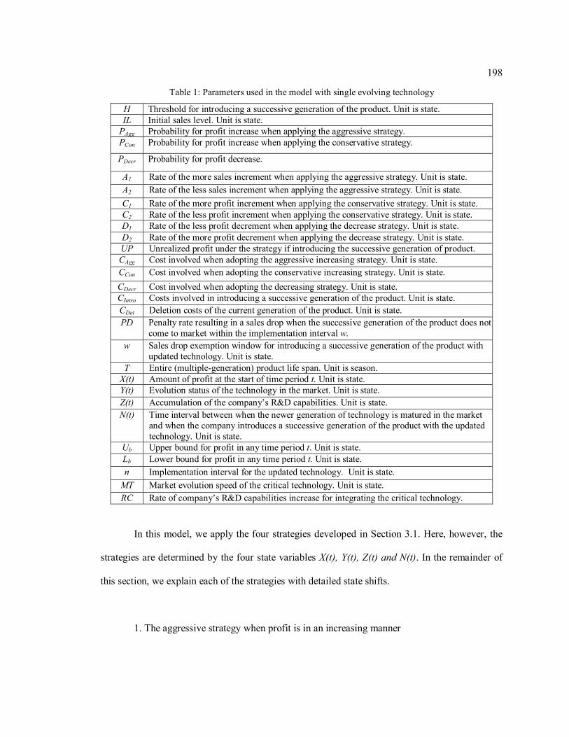
198
Table 1: Parameters used in the model with single evolving technology
H Threshold for introducing a successive generation of the product. Unit is state. IL Initial sales level. Unit is state.
PAgg Probability for profit increase when applying the aggressive strategy. PCon Probability for profit increase when applying the conservative strategy.
PDecr Probability for profit decrease.
A1 Rate of the more sales increment when applying the aggressive strategy. Unit is state. A2 Rate of the less sales increment when applying the aggressive strategy. Unit is state. C1 Rate of the more profit increment when applying the conservative strategy. Unit is state. C2 Rate of the less profit increment when applying the conservative strategy. Unit is state. D1 Rate of the less profit decrement when applying the decrease strategy. Unit is state. D2 Rate of the more profit decrement when applying the decrease strategy. Unit is state. UP Unrealized profit under the strategy if introducing the successive generation of product. CAgg Cost involved when adopting the aggressive increasing strategy. Unit is state. CCon Cost involved when adopting the conservative increasing strategy. Unit is state. CDecr Cost involved when adopting the decreasing strategy. Unit is state. CIntro Costs involved in introducing a successive generation of the product. Unit is state. CDet Deletion costs of the current generation of the product. Unit is state. PD Penalty rate resulting in a sales drop when the successive generation of the product does not
come to market within the implementation interval w. w Sales drop exemption window for introducing a successive generation of the product with
updated technology. Unit is state. T Entire (multiple-generation) product life span. Unit is season.
X(t) Amount of profit at the start of time period t. Unit is state. Y(t) Evolution status of the technology in the market. Unit is state. Z(t) Accumulation of the company’s R&D capabilities. Unit is state. N(t) Time interval between when the newer generation of technology is matured in the market
and when the company introduces a successive generation of the product with the updated technology. Unit is state.
Ub Upper bound for profit in any time period t. Unit is state. Lb Lower bound for profit in any time period t. Unit is state. n Implementation interval for the updated technology. Unit is state.
MT Market evolution speed of the critical technology. Unit is state. RC Rate of company’s R&D capabilities increase for integrating the critical technology.
In this model, we apply the four strategies developed in Section 3.1. Here, however, the
strategies are determined by the four state variables X(t), Y(t), Z(t) and N(t). In the remainder of
this section, we explain each of the strategies with detailed state shifts.
1. The aggressive strategy when profit is in an increasing manner

199
)1()1(
2
11
AggAgg
AggAgg
PyprobabilitwithACxPyprobabilitwithACx
tX
where A1 > A2.
(Eq. 3)
MTytY )1(1 (Eq. 4)
RCztZ )1(1 (Eq. 5)
1110
)1(1 yIfnyIf
tN (Eq. 6)
When a company applies the aggressive strategy to the current generation of the product,
profit rises significantly. In addition, the levels of both the technology in the market and the
company’s R&D capabilities increase following a certain pattern. In our analysis, we let them
both start at the initial conceptual state 0 and move toward being fully prepared at state 1. Time
interval N(t) is dependent on the status of the technology evolution level in the market; it starts
recording only when the newer generation of technology has become mature.
Therefore, according to the evolutionary status of the technology in the market, there are
three different stochastic functions that can be developed for acquiring the expected optimal
profit when choosing the aggressive strategy. When the next generation product is still in
development, choosing the aggressive strategy will simply highly increase the profit; the expected
profit for this scenario is shown in Equation 3-22. However, when the new generation of

200
technology is ready, two different situations may exist. If the company does not release the new
generation within the sales drop exemption window w, selecting the aggressive strategy will cost
it an amount of sales drop equaling a multiple of the length of time over w (See Equation 3-23).
Otherwise, the company will gain only the maximum margin of profit without suffering any
additional cost or loss (See Equation 3-24).
If Y(t) < 1,
)1,0,,,()1(
)1,0,,,(),,,,(
2
11
tRCzMTyACxFPtRCzMTyACxFPtnzyxV
AggAgg
AggAgg
(Eq. 7)
Otherwise,
If N(t) ≤ w,
)1,1,,,()1(
)1,1,,,(),,,,(
2
11
tnRCzMTyACxFPtnRCzMTyACxFPtnzyxV
AggAgg
AggAgg
(Eq. 8)
Otherwise,
PDwntnRCzMTyACxFPtnRCzMTyACxFPtnzyxV
AggAgg
AggAgg
)()1,1,,,()1(
)1,1,,,(),,,,(
2
11
(Eq. 9)
2. The conservative strategy when profit is in an increasing manner
)1(
)1(2
12
ConCon
ConCon
PyprobabilitwithCCxPyprobabilitwithCCx
tX

201
Where C1 > C2.
(Eq. 10)
MTytY )1(2 (Eq. 11)
RCztZ )1(2 (Eq. 12)
1110
)1(2 yIfnyIf
tN (Eq. 13)
Selecting the conservative increasing strategy presents situations similar to those
developed from selecting the aggressive strategy. Again, there are three equal scenarios. Equation
3-29 represents the situation in which the new generation of technology is not matured. Equation
3-30 and Equation 3-31 represent the situation occurring when the updated technology comes to
market and the company is not able to introduce the successive generation of product with the
updated technology within (Eq. 30) and beyond (Eq. 31) the sales drop exemption window (w).
If Y(t) < 1,
)1,0,,,()1()1,0,,,(),,,,(
2
12
tRCzMTyCCxFPtRCzMTyCCxFPtnzyxV
ConCon
ConCon
(Eq. 14)
Otherwise,
If N(t) ≤ w,

202
)1,1,,,()1()1,1,,,(),,,,(
2
12
tnRCzMTyCCxFPtnRCzMTyCCxFPtnzyxV
ConCon
ConCon
(Eq. 15)
Otherwise,
PDwntnRCzMTyCCxFPtnRCzMTyCCxFPtnzyxV
ConCon
ConCon
)()1,1,,,()1()1,1,,,(),,,,(
2
12
(Eq. 16)
3. The strategy for profit drop
)1(
)1(2
13
DecrDecr
DecrDecr
PyprobabilitwithDCxPyprobabilitwithDCx
tX
where D1 < D2
(Eq. 17)
MTytY )1(3 (Eq. 18)
RCztZ )1(3 (Eq. 19)
1110
)1(3 yIfnyIf
tN (Eq. 20)
Selecting the conservative increasing strategy also presents situations similar to those of
the previous two strategies. However, it illustrates the inverse manner with profit decrease. The
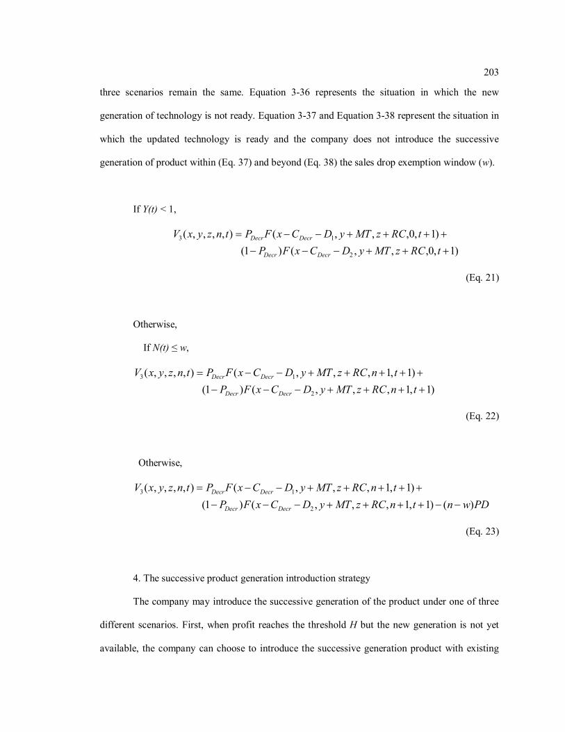
203
three scenarios remain the same. Equation 3-36 represents the situation in which the new
generation of technology is not ready. Equation 3-37 and Equation 3-38 represent the situation in
which the updated technology is ready and the company does not introduce the successive
generation of product within (Eq. 37) and beyond (Eq. 38) the sales drop exemption window (w).
If Y(t) < 1,
)1,0,,,()1()1,0,,,(),,,,(
2
13
tRCzMTyDCxFPtRCzMTyDCxFPtnzyxV
DecrDecr
DecrDecr
(Eq. 21)
Otherwise,
If N(t) ≤ w,
)1,1,,,()1()1,1,,,(),,,,(
2
13
tnRCzMTyDCxFPtnRCzMTyDCxFPtnzyxV
DecrDecr
DecrDecr
(Eq. 22)
Otherwise,
PDwntnRCzMTyDCxFPtnRCzMTyDCxFPtnzyxV
DecrDecr
DecrDecr
)()1,1,,,()1()1,1,,,(),,,,(
2
13
(Eq. 23)
4. The successive product generation introduction strategy
The company may introduce the successive generation of the product under one of three
different scenarios. First, when profit reaches the threshold H but the new generation is not yet
available, the company can choose to introduce the successive generation product with existing
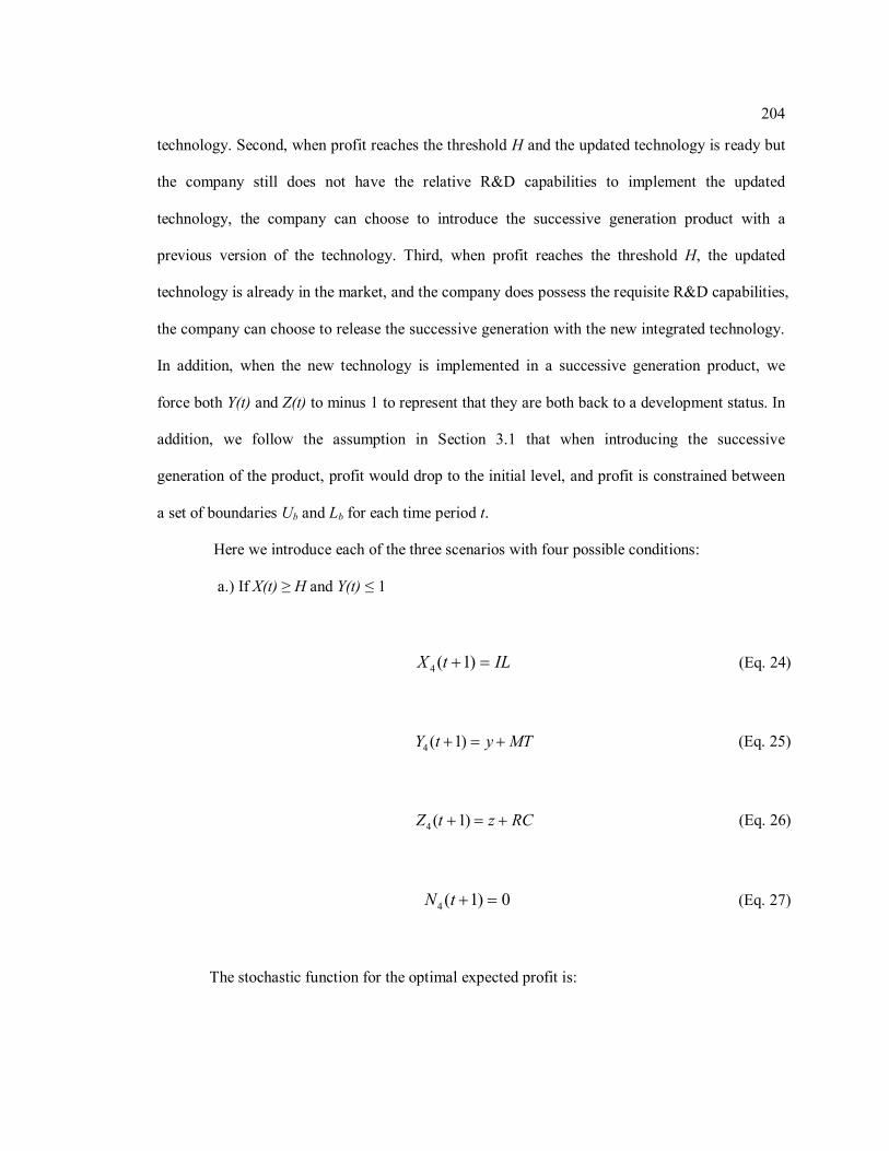
204
technology. Second, when profit reaches the threshold H and the updated technology is ready but
the company still does not have the relative R&D capabilities to implement the updated
technology, the company can choose to introduce the successive generation product with a
previous version of the technology. Third, when profit reaches the threshold H, the updated
technology is already in the market, and the company does possess the requisite R&D capabilities,
the company can choose to release the successive generation with the new integrated technology.
In addition, when the new technology is implemented in a successive generation product, we
force both Y(t) and Z(t) to minus 1 to represent that they are both back to a development status. In
addition, we follow the assumption in Section 3.1 that when introducing the successive
generation of the product, profit would drop to the initial level, and profit is constrained between
a set of boundaries Ub and Lb for each time period t.
Here we introduce each of the three scenarios with four possible conditions:
a.) If X(t) ≥ H and Y(t) ≤ 1
ILtX )1(4 (Eq. 24)
MTytY )1(4 (Eq. 25)
RCztZ )1(4 (Eq. 26)
0)1(4 tN (Eq. 27)
The stochastic function for the optimal expected profit is:

205
DetCUPtRCzMTyILFtpzyxV )1,0,,,(),,,,(4
(Eq. 28)
b.) If HtX )( , Y(t) ≥ 1 and Z(t) < 1,
ILtX )1(4 (Eq. 29)
MTytY )1(4 (Eq. 30)
RCztZ )1(4 (Eq. 31)
1)1(1 ntN (Eq. 3-32)
The stochastic function for the optimal expected profit is:
If N(t) > w
DetCUPtnRCzMTyILFtnzyxV )1,1,,,(),,,,(4
(Eq. 3-33)
Otherwise
PDwnCUPtnRCzMTyILFtpzyxV Det )()1,1,,,(),,,,(4
(Eq. 3-34)
c.) If HtX )( , Y(t) ≥ 1 and Z(t) ≥ 1,

206
ILtX )1(4 (Eq. 3-35)
1)1(4 MTytY (Eq. 3-36)
1)1(4 RCztZ (Eq. 3-37)
0)1(1 tN (Eq. 3-38)
The stochastic function for the expected profit is:
DetCUPtRCzMTyILFtpzyxV )1,0,1,1,(),,,,(4
(Eq. 3-39)
In addition, for each time period t, since F(x, y, z, n, t) is the maximum expected profit
given that X(t) = x, Y(t) = y, Z(t) = z, N(t) = n, F(x, y, z, n, t) should be assigned the maximal
expected revenue values for the following four strategies:
F(x, y, z, n, t) = max {V1(x, y, z, n,), V2(x, y, z, n,), V3(x, y, z, n,), V4(x, y, z, n,)}
(Eq. 3-40)
In this study, we do not provide the case study for this basic model with technology
evolution concern. From the IBM mainframe system case study, we do not have technology
related information from the data. However, in Chapter 4, we formulate the technology evolution

207
model for the cannibalization scenario and provide a case study implementing the sales data from
the Apple iPhone product line. In fact, technology evolution model could be considered an
extension from this model. When removing the cannibalization settings, the technology evolution
model could generate the same results as this model.

VITA
Chun-yu Lin
Chun-yu Lin was born in Taiwan on June 5, 1982. He received his Bachelor degree from
National Chao-Tung University, Hsinchu, Taiwan in 2004. He came to Pennsylvania State
University for his Master and PhD study in 2006, and received his Master degree in 2009. During
his PhD study, he has published several research papers in academic journals and presented his
works in several international conferences. In 2012, his publication “Application of Dynamic
State Variable Models on Multiple-Generation Product Lines with Cannibalization across
Generations” received the best paper award from the Engineering Management (EM) track of the
Industrial and Systems Engineering Research Conference (ISERC).