the pennsylvania state · pdf filethe pennsylvania state university the graduate school...
TRANSCRIPT
The Pennsylvania State University
The Graduate School
Department of Aerospace Engineering
REAL-TIME PATH PLANNING AND AUTONOMOUS CONTROL FOR HELICOPTER
AUTOROTATION
A Dissertation in
Aerospace Engineering
by
Thanan Yomchinda
2013 Thanan Yomchinda
Submitted in Partial Fulfillment
of the Requirements
for the Degree of
Doctor of Philosophy
May 2013

The dissertation of Thanan Yomchinda was reviewed and approved* by the following:
Joseph F. Horn
Associate Professor of Aerospace Engineering
Dissertation Co-Advisor
Co-Chair of Committee
Jacob W. Langelaan
Associate Professor of Aerospace Engineering
Dissertation Co-Advisor
Co-Chair of Committee
Edward C. Smith
Professor of Aerospace Engineering
Christopher D. Rahn
Professor of Mechanical Engineering
George A. Lesieutre
Professor of Aerospace Engineering
Head of the Department of Aerospace Engineering
*Signatures are on file in the Graduate School

iii
ABSTRACT
Autorotation is a descending maneuver that can be used to recover helicopters in the
event of total loss of engine power; however it is an extremely difficult and complex maneuver.
The objective of this work is to develop a real-time system which provides full autonomous
control for autorotation landing of helicopters. The work includes the development of an
autorotation path planning method and integration of the path planner with a primary flight
control system. The trajectory is divided into three parts: entry, descent and flare. Three different
optimization algorithms are used to generate trajectories for each of these segments. The primary
flight control is designed using a linear dynamic inversion control scheme, and a path following
control law is developed to track the autorotation trajectories. Details of the path planning
algorithm, trajectory following control law, and autonomous autorotation system implementation
are presented. The integrated system is demonstrated in real-time high fidelity simulations.
Results indicate feasibility of the capability of the algorithms to operate in real-time and of the
integrated systems ability to provide safe autorotation landings. Preliminary simulations of
autonomous autorotation on a small UAV are presented which will lead to a final hardware
demonstration of the algorithms.
iv
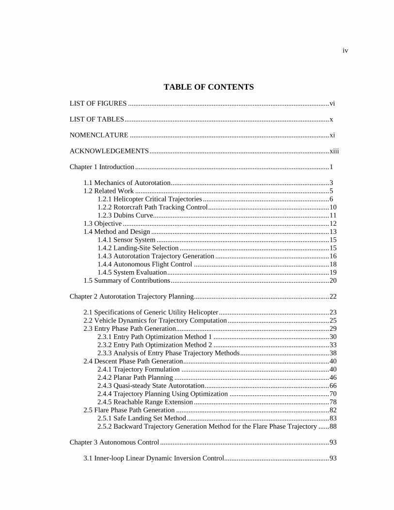
TABLE OF CONTENTS
LIST OF FIGURES ................................................................................................................. vi
LIST OF TABLES ................................................................................................................... x
NOMENCLATURE ................................................................................................................ xi
ACKNOWLEDGEMENTS ..................................................................................................... xiii
Chapter 1 Introduction ............................................................................................................. 1
1.1 Mechanics of Autorotation ......................................................................................... 3 1.2 Related Work ............................................................................................................. 5
1.2.1 Helicopter Critical Trajectories ....................................................................... 6 1.2.2 Rotorcraft Path Tracking Control .................................................................... 10 1.2.3 Dubins Curve................................................................................................... 11
1.3 Objective .................................................................................................................... 12 1.4 Method and Design .................................................................................................... 13
1.4.1 Sensor System ................................................................................................. 15 1.4.2 Landing-Site Selection .................................................................................... 15 1.4.3 Autorotation Trajectory Generation ................................................................ 16 1.4.4 Autonomous Flight Control ............................................................................ 18 1.4.5 System Evaluation ........................................................................................... 19
1.5 Summary of Contributions ......................................................................................... 20
Chapter 2 Autorotation Trajectory Planning ............................................................................ 22
2.1 Specifications of Generic Utility Helicopter .............................................................. 23 2.2 Vehicle Dynamics for Trajectory Computation ......................................................... 25 2.3 Entry Phase Path Generation ...................................................................................... 29
2.3.1 Entry Path Optimization Method 1 ................................................................. 30 2.3.2 Entry Path Optimization Method 2 ................................................................. 33 2.3.3 Analysis of Entry Phase Trajectory Methods .................................................. 38
2.4 Descent Phase Path Generation .................................................................................. 40 2.4.1 Trajectory Formulation ................................................................................... 40 2.4.2 Planar Path Planning ....................................................................................... 46 2.4.3 Quasi-steady State Autorotation ...................................................................... 66 2.4.4 Trajectory Planning Using Optimization ........................................................ 70 2.4.5 Reachable Range Extension ............................................................................ 78
2.5 Flare Phase Path Generation ...................................................................................... 82 2.5.1 Safe Landing Set Method ................................................................................ 83 2.5.2 Backward Trajectory Generation Method for the Flare Phase Trajectory ...... 88
Chapter 3 Autonomous Control ............................................................................................... 93
3.1 Inner-loop Linear Dynamic Inversion Control........................................................... 93
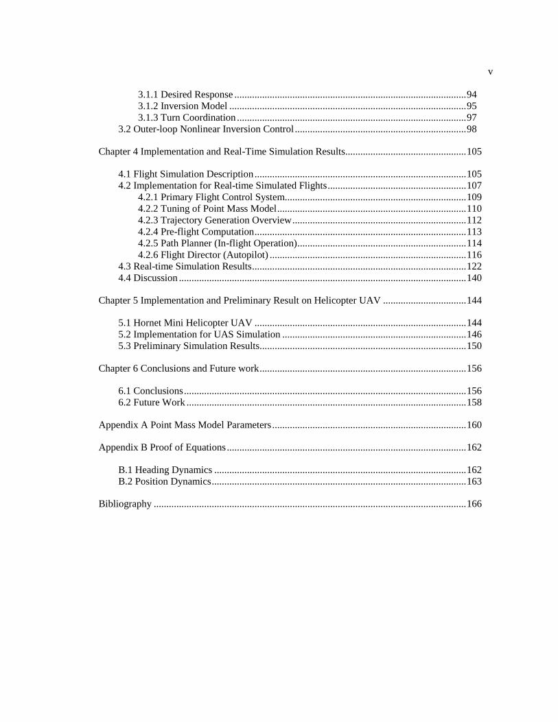
v
3.1.1 Desired Response ............................................................................................ 94 3.1.2 Inversion Model .............................................................................................. 95 3.1.3 Turn Coordination ........................................................................................... 97
3.2 Outer-loop Nonlinear Inversion Control .................................................................... 98
Chapter 4 Implementation and Real-Time Simulation Results ................................................ 105
4.1 Flight Simulation Description .................................................................................... 105 4.2 Implementation for Real-time Simulated Flights ....................................................... 107
4.2.1 Primary Flight Control System........................................................................ 109 4.2.2 Tuning of Point Mass Model ........................................................................... 110 4.2.3 Trajectory Generation Overview ..................................................................... 112 4.2.4 Pre-flight Computation .................................................................................... 113 4.2.5 Path Planner (In-flight Operation) ................................................................... 114 4.2.6 Flight Director (Autopilot) .............................................................................. 116
4.3 Real-time Simulation Results ..................................................................................... 122 4.4 Discussion .................................................................................................................. 140
Chapter 5 Implementation and Preliminary Result on Helicopter UAV ................................. 144
5.1 Hornet Mini Helicopter UAV .................................................................................... 144 5.2 Implementation for UAS Simulation ......................................................................... 146 5.3 Preliminary Simulation Results.................................................................................. 150
Chapter 6 Conclusions and Future work .................................................................................. 156
6.1 Conclusions ................................................................................................................ 156 6.2 Future Work ............................................................................................................... 158
Appendix A Point Mass Model Parameters ............................................................................. 160
Appendix B Proof of Equations ............................................................................................... 162
B.1 Heading Dynamics .................................................................................................... 162 B.2 Position Dynamics ..................................................................................................... 163
Bibliography ............................................................................................................................ 166

vi
LIST OF FIGURES
Figure 1-1. Phases of Autorotation Landing Flight [11, 12]. ................................................... 2
Figure 1-2. Variation of force on the blades in autorotation [9]. ............................................. 3
Figure 1-3. Typical power required versus airspeed curve for a helicopter [4]. ...................... 5
Figure 1-4. Framework for an autonomous autorotation control system. ................................ 14
Figure 2-1. Schematic of path planning system. ...................................................................... 22
Figure 2-2. Principal dimensions of the generic utility helicopter (similar to UH-60) [88] .... 25
Figure 2-3. Definitions of the coordinates and key parameters of the helicopter point mass
model. ............................................................................................................................... 28
Figure 2-4. Definitions of the aircraft pitch and bank angles. ................................................. 28
Figure 2-5. Definitions of the aircraft position and heading, . .............................................. 29
Figure 2-6. Example of entry path input solution for 100 knots airspeed from the first
method, sec, N = 400 nodes, and K = 9 nodes. ................................................ 32
Figure 2-7. Optimization process for entry path method 2. ..................................................... 34
Figure 2-8. Example of an entry path input solution for 100 knots airspeed from the
second method. ................................................................................................................. 36
Figure 2-9. Example of an entry path input solution from the second method for the initial
hover case. ........................................................................................................................ 37
Figure 2-10. Comparison of path solutions from the two optimization methods. ................... 39
Figure 2-11. Turning segment in the modified Dupins’ paths. ................................................ 42
Figure 2-12. Definitions of points and segments in the modified Dupins’ paths. ................... 43
Figure 2-13. Descent phase autorotation trajectory generating process................................... 45
Figure 2-14. Example of descent phase autorotation trajectory. .............................................. 46
Figure 2-15. Definitions of the case with achieved bank angle (upper) and the case with
insufficient time (lower). .................................................................................................. 48
Figure 2-16. Definitions of the parameters in the geometry-based search method.................. 53
Figure 2-17. Geometry-based search method. ......................................................................... 56
Figure 2-18. Three-point pattern and local minimum. ............................................................. 63

vii
Figure 2-19. Summary of iterative searching method. ............................................................. 64
Figure 2-20. Horizontal path in no-wind condition for ...................................................................................................................... 65
Figure 2-21. Horizontal path in the presence of 10-feet-per-second wind from the west for
. .................................................................... 66
Figure 2-22. Example of quasi-steady autorotation solutions for straight flight with
various accelerations. (Red: ax,l = 0.1g, Blue: ax,l = 0, Green: ax,l = -0.1g) .................... 69
Figure 2-23. Example of a quasi-steady autorotation trajectory. ............................................. 73
Figure 2-24. Time histories of the no-wind scenario. .............................................................. 74
Figure 2-25. Example of a quasi-steady autorotation trajectory in constant wind. .................. 75
Figure 2-26. Time histories of the constant wind scenario. ..................................................... 76
Figure 2-27. Time histories of the constant wind scenario. (Continued) ................................. 77
Figure 2-28. Modified planar-path search for a two-segment descent path. ............................ 79
Figure 2-29. Example of a two-segment quasi-steady autorotation trajectory in constant
wind. ................................................................................................................................. 80
Figure 2-30. Time histories of two-segment quasi-steady autorotation trajectory in the
constant wind scenario. .................................................................................................... 81
Figure 2-31. Example of reachable area for autorotation flight path. ...................................... 82
Figure 2-32. Example of a safe landing set. [11, 12] ............................................................... 84
Figure 2-33. Example of a flare phase trajectory solution. ...................................................... 87
Figure 2-34. Flare autorotation landing technique and computation process of the flare
trajectory. ......................................................................................................................... 88
Figure 2-35. Example of a flare phase trajectory solution from the backward trajectory
generation algorithm. ....................................................................................................... 92
Figure 3-1. Schematic of an autonomous control and path-planning system. ......................... 93
Figure 3-2. Schematic of the linear dynamic inversion control system for primary flight
control. ............................................................................................................................. 94
Figure 3-3. Autonomous autorotation control diagram............................................................ 99

viii
Figure 4-1. Simulation process diagram. ................................................................................. 106
Figure 4-2. Network communication between the autonomous system and the flight
simulator........................................................................................................................... 108
Figure 4-3. Correlations between the point mass model and the FLIGHTLAB model. .......... 111
Figure 4-4. Process of path planner. ........................................................................................ 116
Figure 4-5. Process of the flight director. ................................................................................ 118
Figure 4-6. Touchdown conditions of simulated autonomous autorotation flights. ................ 123
Figure 4-7. Trajectory of the autorotation landing flight in case 1. ......................................... 127
Figure 4-8. Time histories of the autorotation landing flight in case 1. ................................... 128
Figure 4-9. Deviations in the trajectory of the autorotation landing flight in case 1. .............. 129
Figure 4-10. Trajectory of the autorotation landing flight in case 2. ....................................... 130
Figure 4-11. Time histories of the autorotation landing flight in case 2. ................................. 131
Figure 4-12. Deviations in the trajectory of the autorotation landing flight in case 2. ............ 132
Figure 4-13. Trajectory of the autorotation landing flight in case 3. ....................................... 133
Figure 4-14. Time histories of the autorotation landing flight in case 3. ................................. 134
Figure 4-15. Deviations in the trajectory of the autorotation landing flight in case 3. ............ 135
Figure 4-16. Example of autonomous autorotation flights in steady wind. ............................. 136
Figure 4-17. Example of rotor flapping angles in autonomous autorotation landing flights. .. 138
Figure 4-18. Example of rotor flapping angles during flare-phase autorotation. ..................... 139
Figure 4-19. Computation time for the descent-phase trajectory. ............................................ 140
Figure 5-1. Adaptive Flight’s Hornet Mini UAS [90] ............................................................. 145
Figure 5-2. Schematic of autonomous autorotation system implementation on UAS
system .............................................................................................................................. 147
Figure 5-3. Correlation between point mass model and Hornet Mini UAS model .................. 148
Figure 5-4. Flight path of autorotation landing flight in ground control station interface
for case 1 .......................................................................................................................... 152
Figure 5-5. Response and trajectory control histories for case 1 ............................................. 153

ix
Figure 5-6. Flight path of autorotation landing flight in ground control station interface
for case 2 .......................................................................................................................... 154
Figure 5-7. Response and trajectory control histories for case 2 ............................................. 155

x
LIST OF TABLES
Table 2-1. Properties of generic utility helicopter ................................................................... 24
Table 2-2. Turning segment categorization ............................................................................. 59
Table 2-3. Performance of the iterative method for Case C .................................................... 61
Table 2-4. Performance of the iterative method for Case D .................................................... 62
Table 4-1. Parameters of primary flight control ...................................................................... 109
Table 4-2. Simulated flight test data points ............................................................................. 110
Table 4-3. Quasi-steady autorotation data points generated for the approximation function .. 114
Table 4-4. Summary of performance results ............................................................................ 125
Table 5-1. Properties of Hornet Mini UAS .............................................................................. 145
Table 5-2. Quasi-steady autorotation data points generated for the UAS implementation ...... 149
Table 5-3. Summary of results from representative cases ....................................................... 150
Table A-1. Additional parameters for generic utility helicopter .............................................. 160
Table A-2. Additional parameters for Hornet Mini UAS ........................................................ 161

xi
NOMENCLATURE
A, B State and control matrices in aircraft state space model
Acceleration components of aircraft
Cost function
Rotor thrust coefficient
Rotor blade profile drag coefficient
Aerodynamic drag force
Rotor polar moment of inertia
Gravitational acceleration
k Iteration number
m Mass of aircraft
n Number of turn in turning segment of descent phase trajectory
p, q, r Aircraft angular velocity
R Rotor radius
T Rotor thrust
u, v, w Velocity components
u Parametric control input vector
V Airspeed
W Aircraft weight
x, y, z North position, East position and vertical position of aircraft
x, v Helicopter state and control vectors
Bank angle, pitch angle and heading of aircraft
Rotor solidity
Rotor power efficiency factor
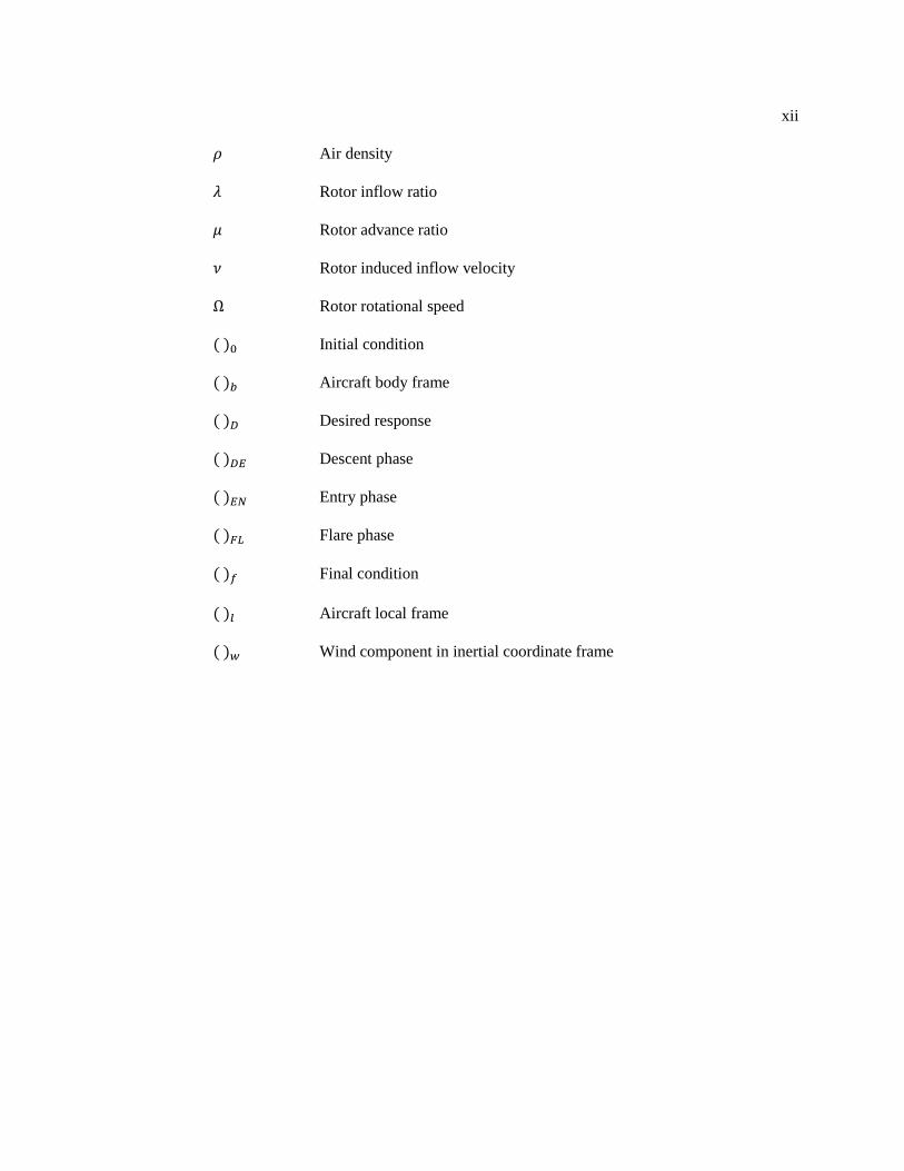
xii
Air density
Rotor inflow ratio
Rotor advance ratio
Rotor induced inflow velocity
Rotor rotational speed
Initial condition
Aircraft body frame
Desired response
Descent phase
Entry phase
Flare phase
Final condition
Aircraft local frame
Wind component in inertial coordinate frame

xiii
ACKNOWLEDGEMENTS
First of all, I would like to express my gratitude to my two co-advisors, Dr. Joseph F.
Horn and Dr. Jack W. Langelaan, for advice, support, opportunities and academic guidance given
throughout my Ph.D. study. I would also like to thank my committee members, Dr. Edward C.
Smith and Dr. Christopher D. Rahn for their comments and suggestions.
I also thank my fellow Penn State students and colleagues at Vertical Lift Research
Center of Excellence for their help, support, and friendship. Special thanks to Mark DeAngelo
for feedbacks on this dissertation.
Finally and most importantly, I would like to express my deepest gratitude to my parents,
Thanachai and Ladawan Yomchinda. I would not be where I am right now if it was not for their
love, support, encouragement, and their attempt and eagerness to see me pursue my dream.

Chapter 1
Introduction
With the increased focus on the use of both manned and unmanned rotorcraft for safety-
critical tasks such as resupply, casualty evacuation, and other civil applications, response in the
event of failures has become an important issue. Even though rotorcraft technology has
significantly improved in terms of reliability in recent years, emergencies, such as engine failure
or the total loss of engine power, do occur [1, 2]. Yet, emergency situations such as these are
recoverable via autorotation. However, autorotation is an extremely difficult and complex
maneuver. Even for human pilots, it is a significant concern [3-5].
Helicopter autorotation is a descending maneuver in which the rotor system is disengaged
from the engine. The rotor blades are driven solely by the oncoming upward flow through the
main rotor. This is a self-sustained maneuver in which the potential energy of altitude is
converted into the energy required by the rotor to provide lift and control to the rotorcraft [6-10].
A typical autorotation scenario is shown in Figure 1-1. Beginning at the moment of engine
failure, the autorotation process requires a reduction of the rotor collective blade pitch angle in
order to maintain the rotor’s rotational energy and produce an upward flow through the rotor. The
helicopter nose must also be pushed down to initiate an autorotation descent. In the descent
phase, the pilot must look for landing sites and maneuver the aircraft in order to prepare for
landing on a suitable site. Typically, the descent will either minimize the descent rate thereby
maximizing the time the pilot has to look for a landing site, or it will maximize the gliding range
thereby giving the pilot the largest possible number of landing sites from which to choose. The
most critical and difficult phase is known as the flare. During this phase, the energy in the freely
spinning rotor is used to arrest both the descent rate and the forward speed so that a safe

2
touchdown can be executed. In the beginning of flare phase, the helicopter nose must be pulled up
to decelerate the forward speed. The rotor speed can be increased in this maneuver as oncoming
airflow from forward speed is converted into upward flow through the rotor. At a certain altitude,
the collective pitch control must be pulled to generate a decelerating thrust. This collective pitch
control rapidly drops the rotor speed as the rotational energy in the rotor is consumed in the rotor
thrust generation. Before the touchdown is occurred, the pitch attitude must be reduced to a
suitable range so that the tail rotor is clear from the ground contact and the touchdown impact is
evenly distributed to the landing gears. During the flare, the collective pitch control must be
timed properly: the result can be rotor stall, if the control is initiated too early, or a hard landing if
initiated too late. The maneuver throughout the autorotation flight is also very restricted, as there
is no recoverability if the rotor speed drops below a certain threshold before touchdown.
Figure 1-1. Phases of Autorotation Landing Flight [11, 12].
In responding to this total engine power loss, we could consider other design features,
e.g., providing impact protection for both the pilots and the vehicles. However, a system that
guarantees successful execution of an autorotation landing is the most effective way to minimize
damage to the aircraft and prevent both serious injury and the loss of life. This study focuses on
providing autonomous autorotation landings for helicopters.
Flare Initiation
Engine Failure
Entry
Descent
Flare
3
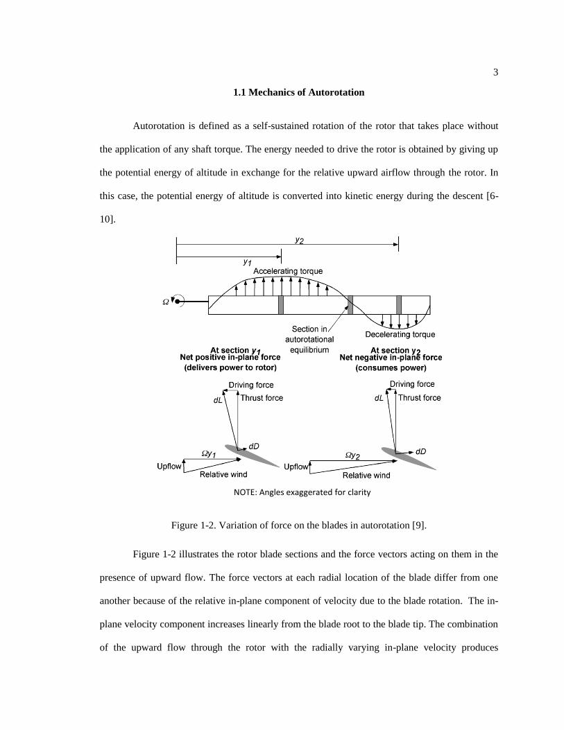
1.1 Mechanics of Autorotation
Autorotation is defined as a self-sustained rotation of the rotor that takes place without
the application of any shaft torque. The energy needed to drive the rotor is obtained by giving up
the potential energy of altitude in exchange for the relative upward airflow through the rotor. In
this case, the potential energy of altitude is converted into kinetic energy during the descent [6-
10].
Figure 1-2. Variation of force on the blades in autorotation [9].
Figure 1-2 illustrates the rotor blade sections and the force vectors acting on them in the
presence of upward flow. The force vectors at each radial location of the blade differ from one
another because of the relative in-plane component of velocity due to the blade rotation. The in-
plane velocity component increases linearly from the blade root to the blade tip. The combination
of the upward flow through the rotor with the radially varying in-plane velocity produces
NOTE: Angles exaggerated for clarity

4
different angles of attack and a different inclination of the aerodynamic force at every radial
location along the blade. In the driving region, the total aerodynamic force is inclined slightly
forward of the axis of rotation and produces the force that accelerates the rotation of the blade. In
the driven region, the forward component of the lift produced at the blade section is offset by the
drag (i.e., the driving force is lower than the drag force), resulting in a total aerodynamic force
that tends to decelerate the rotation of the blade. Between the driven region and the driving
region, there is an equilibrium point. At this point, the total aerodynamic force is aligned with the
axis of rotation and results in neither acceleration nor deceleration. The net torque on the entire
blade is the accumulated torque resultant from all blade sections. The autorotation equilibrium in
the rotor occurs when the combined net torque from all rotor blades results no
acceleration/deceleration to the entire rotor.
In an actual rotorcraft, the engine power is supplied not only to the main rotor but also to
the tail rotor and other power accessories as well. In autorotation, all of those systems are
required for the operation of the rotorcraft. The free-spinning main rotor becomes necessary to
produce a driving torque for the entire system. The autorotation equilibrium then occurs when
combined net torque from the main rotor and other power required systems is zero for the entire
rotorcraft system.
Autorotation is typically performed in a forward flight condition, which requires a lower
descent rate than a pure vertical descent does. Autorotation in a pure vertical descent requires a
transition through the vortex ring state (VRS) region where the rotor intakes its own tip vortices
and experiences a very unsteady inflow. Rotors operating in the VRS region require a large
amount of power. The VRS region is a highly unstable regime and should generally be avoided.
The descent rate required for autorotation with forward speed can be derived from the
power required for level flight in the normal conditions. Figure 1-3 illustrates the required power
from hover to level forward flight for an example helicopter. The higher amount of power

5
required in the normal flight at an airspeed implies a higher descent rate in autorotation at the
same airspeed, and vice versa. The recommended forward speed for autorotation is typically near
the airspeed, which requires minimum power for level flight as the minimum descent rate is
achieved in this airspeed [4].
Figure 1-3. Typical power required versus airspeed curve for a helicopter [4].
1.2 Related Work
The safety of autorotation maneuvers is a significant concern in the rotorcraft
community. A significant amount of research has been conducted with the aim of aiding (for
crewed vehicles) and automating (for unmanned vehicles) descent and landing during
autorotation maneuvers.

6
1.2.1 Helicopter Critical Trajectories
Several studies were conducted to investigate the operational envelopes for helicopter
critical and emergency trajectories using optimization methods. In 1977, Johnson [13] introduced
the approach of solving a helicopter longitudinal autorotation descent and landing problem by
using nonlinear optimal control theory [14]. A helicopter point-mass model including the ground
effect expression by Cheeseman and Bennett [15] and the pilot reaction time lag of 0.75 seconds
was used to represent the dynamics of an OH-58A helicopter with a High Energy Rotor System
(HERS) [16]. A two-point boundary value optimization problem was formulated to find the
control inputs required to bring the vehicle from known initial flight states at the engine failure
point to the ground at minimum velocity. A weighted sum of squared horizontal and vertical
velocity components at touchdown was used for the cost function. Control inputs as a function of
altitude, which corresponded to the minimum cost function value, were found by using a
nonlinear optimal control method. The approach and basic feature of the mathematic model were
verified by a comparison between the analytical solution and the flight test data. A sufficient
correlation to validate the approach was found.
Lee et al. [17-19] improved on Johnson’s work [13] by adding path inequality constraints
on the rotor thrust, which reflected the limited amount of available thrust without stalling the
rotor and maximum sink rate. The control inputs for autorotation landing were solved by using
the Sequential Gradient Restoration Algorithm (SGRA) developed by Miele et al. [20]. Analytical
solutions of the power-off autorotation landing from hover and level-forward flight were
validated by comparing the available flight data from an autorotation flight test program
conducted by the Bell Helicopter Company with the analytical results. The correlation between
the flight test data and the analytical results established the adequacy of the approach and the use
of a point mass model in the optimal helicopter autorotation landing study.

7
Okuno et al. [21-22] used a four-degree-of-freedom longitudinal helicopter model to
analyze autorotation optimal control problems. The prediction of the height-velocity unsafe
boundaries and optimal landing procedures were found by using various performance indices and
a nonlinear control theory. The method was used to find optimal takeoff procedures for Category
A V/STOL operations [23] and validated by using the pilot’s control recorded during flight tests
[24].
Zhao et al. [25-28] investigated several expressions of performance indices for helicopter
takeoff and landing trajectories in one engine inoperative (OEI) situations. An engine power
model was incorporated into the point-mass model in Lee et al. [17]. Bounds on the rotor thrust,
rotor speed, and thrust angle were applied in the formulation of the nonlinear optimal control
problems, and the SGRA was used to find optimal control solutions. The autorotation optimal
control problem was converted into a parameter-optimization problem, and the NPSOL [30]
software package was used to compute numerical solutions in [29].
Carlson et al. [31-34] applied the previous study by Zhao et al. [28] to investigate the
unsafe (avoid) regions of the height-velocity (H-V) envelope and the flight path in the event of
engine failure in XV-15 civil tilt-rotor aircraft. The point-mass model used in previous study [28]
was modified to include a complex nonlinear aerodynamic model to represent the XV-15 civil
tilt-rotor aircraft dynamics. The nonlinear optimal control problems were formulated to minimize
the weighted sum of squared horizontal and vertical velocity components and subject to selected
initial conditions, path constraints, and terminal constraints and used the SGRA to facilitate
numerical solutions to the problems. This method was also used to investigate optimal trajectories
and to establish a height-velocity diagram for the AH-1Z and UH-1Y helicopters [35].
Aponso et al. [36-38] introduced an outline of a real-time autorotation trajectory
optimization method for a helicopter in the event of total power loss, which could be used to
guide an autonomous unmanned helicopter or a remote operator of an unmanned rotorcraft. It

8
could also be used to cue a helicopter pilot through an autorotation landing. The point-mass
model in the work of Zhao et al. [28] was adopted to formulate optimal autorotation problems for
a Bell-206L-4 helicopter. The two-point boundary value problem from a previous study [31-34]
was transformed into a parameter-optimization problem by using a direct method of optimization.
The continuous path was discretized into nodes. The aircraft states and controls at each discrete
point were the parameters in the optimization method, which were solved in order to satisfy the
dynamics and constraints. The direct collocation method used to this work was found to have a
better convergence radius with a wider range of initial guesses than other optimization methods;
however, the direct collocation method it is at a disadvantage in regard to the dimension of the
problem, which was large due to discretization.
Floros [39] extended the work of Johnson [13] and Lee et al. [17-19]. The autorotation
optimal control problem was modified by adding rate controls and additional thrust limits and
altitude constraints on the optimal control procedure in order to obtain better representations of
the pilot’s reaction and the helicopter’s motion. The analytical solutions were validated against
autorotation-landing flight data from hover and forward-flight initial conditions.
Tierney [11, 12] focused on a real-time application of the flare-phase trajectory planning
for the autorotation-landing problem. The safe landing set, defined as the region in the helicopter
state space from which a safe flare to touchdown is guaranteed to exist, was computed in this
work. The states incorporated in the safe landing set comprise the flare initiation point (distance
to and height above the desired touchdown point), airspeed, descent rate, and rotor speed. The
parameter-optimization method introduced by Aponso et al. [36] was modified in order to have
better computational speed by reducing the problem dimension. The altitude discretization was
implemented to specify the end point (touchdown altitude was defined, but touchdown time was
not). The control inputs were parameterized by using a spline function, which reduces the number
of parameters and implicitly forces some smoothness on the inputs. The point-mass model in

9
Aponso et al. [36] was used to formulate of the parameter-optimization algorithm. The upper and
lower limits on the states and controls were applied during the entire flight. The safe touchdown
conditions were decided from the final position, forward speed, descent rate, and pitch angle. The
method was applied to find solutions for a large number of initial conditions, and those that were
solved were used to indicate the safe landing set region. The safe landing set from the study could
be used as the target region for the previous autorotation phases (entry and descent phases), as
any autorotation descent passing through the safe landing set thus has a guaranteed solution to the
problem of flare trajectory planning.
Bibik et al. [40] used a comprehensive eight-degree-of-freedom helicopter model to find
the optimal control for AEI autorotation landing, OEI landing, and OEI takeoff for a PZL Mi-2
Plus helicopter. A discrete time-adaptive optimal-control algorithm was developed to find
helicopter control surface inputs (the main rotor collective pitch angle, the main rotor lateral and
longitudinal cyclic pitch angles, and the tail rotor collective pitch angle) for specified engine
failure conditions. The MATLAB FMINCON was utilized to obtain solutions of the optimal
control problems.
Taamallah [41, 42] derived optimal autorotation trajectories for a helicopter Unmanned
Aerial Vehicle (UAV). A three-dimensional nonlinear helicopter model was used to compute the
height-velocity diagram. An obstacle avoidance capability was included in the computation of the
optimal autorotation trajectories by incorporating the three-dimensional obstacle information in
path constraints. A direct optimal control method was used to solve the optimal control problem.
The power-off autorotation landing problem has also been investigated by using a
machine-learning approach. Lee et al. [43] applied a Neural Network technique to the
autorotation problem. A reinforcement learning algorithm was used to train a controller for
autorotation. The point-mass model of a modified OH-58A by Johnson [13] was used to simulate

10
helicopter flight dynamics in a cost function. The trained controller produced optimal autorotation
landing profiles for the initial conditions of hover and low forward speed at a low altitude.
Dalamagkidis et al. [44, 45] developed a nonlinear model predictive controller to perform
vertical autorotation autonomously. A recurrent neural network was augmented to the controller
with the purpose of finding an optimal control sequence for vertical autorotation flight. Training
based on repeated simulated autorotation trials were then performed and led the trained controller
to achieve the stated objective.
Abbeel et al. [46] investigated an autonomous autorotation landing of a remotely
controlled helicopter. A thirteen-state, rigid-body model, which included positions, velocities,
attitude, angular rate and rotor dynamics, as well as four general control inputs were used to
represent the autorotation dynamics of a radio-controlled helicopter (an XCell Tempest). The
target trajectory was obtained by idealizing the autorotation trajectories performed by expert
human pilots. A linear quadratic regulator (LQR) controller was designed for autonomous
autorotation. The approach was implemented on an XCell Tempest RC helicopter, and a
successful autonomous autorotation landing on an open field was executed.
1.2.2 Rotorcraft Path Tracking Control
Trajectory planning and path tracking control are the basic functions of an autonomous
rotorcraft. Normally, a rotorcraft trajectory is a path that has been planned before a flight and
generated based on the mission and known obstacles. The path is often executed using a waypoint
method. A smooth flight based on pre-planned path and accounted for wind [47] or inflight-
realized obstacles [48-50] can later be generated during flight time. Trajectory planning which
provides real-time response to change in environment or to anomalous situation for aircraft is

11
usually based on the Dubins’ concept [51, 52], which uses simple geometric figures, such as
circles and straight lines, to compose paths with a bounded aircraft turning radius [47, 53, 54].
The path tracking control in rotorcraft is commonly divided into an inner loop control
that controls the rotorcraft attitude and an outer loop control that tracks the rotorcraft movement
in the desired trajectory. Johnson et al. [55, 56] used dynamics inversion and a neural network to
improve the performance of the attitude control system, and implemented a dynamic inversion-
based outer loop control to improve the tracking performance for aggressive maneuvers.
Bayraktar et al. [57] investigated the feasibility of landing a helicopter UAV on an
inclined surface. The landing trajectory was generated before the flight. Tracking controls were
developed to command the attitude control of the remote-control helicopter. Tracking control
laws were different for each flight phase (hover, approach and pitch-up), and the control law used
during the flight was selected by using specified thresholds and/or via manual commands.
1.2.3 Dubins Curve
The Dubins curve [51, 52] is a popular method in modern trajectory planning. It is very
useful for planning a trajectory in two-dimensional space for an object with a constant velocity
and turn rate (the so called Dubins car). Trajectories between two points with specified initial and
final headings can be simply constructed using basic geometries (circles and a straight line). Eight
different paths can be generated from six path types. The six path types are Left-turn-Straight-
Left-turn (LSL), Left-turn-Straight-Right-turn (LSR), Right-turn-Straight-Right-turn (RSR),
Right-turn-Straight-Left-turn (RSL), Right-turn-Left-turn-Right-turn (RLR), and Left-turn-Right-
turn-Left-turn (LRL). Two different paths can be produced from each RLR and LRL path type.
The method results in the shortest path and up to seven alternative paths. The Dubins curve is
12
considered to be one of the most robust methods in trajectory generation because the concept is
guaranteed to produce at least four paths, one of which is the minimum distance solution.
1.3 Objective
The primary focus of this work is to improve the safety of autorotation landings by
developing: (1) real-time trajectory-planning algorithms for autorotation initiation, descent, and
landing; and (2) an autonomous control system for autorotation landing to be used on board a
helicopter. To be useful in practical applications, the method must be reliable, robust, and
computationally efficient. The vehicle’s properties and structural limitations are essentially
incorporated into the trajectory-planning and autonomous control methods in order to ensure the
safety and feasibility of autonomous autorotation landing.
The objectives of this research are as follows:
1) To develop a descent-trajectory planning algorithm
1.1) Enable real-time computation while accounting for wind as well as vehicle
state, dynamics and structural constraints;
1.2) Bring the aircraft to land at a specified location;
1.3) Allow the aircraft to vary its speed along the path; and
1.4) Maneuver the aircraft within acceptable attitude, angular rate, and angular
acceleration.
2) To develop autonomous controls capable of maneuvering unmanned vehicles along
every autorotation path solution.
3) To develop a method that integrates the previous two objectives into a system to
provide full autonomous autorotation landings for a helicopter. This objective also
includes:

13
3.1) implementing safe flare initiation and a flare trajectory-planning method [11, 12]
for real-time applications; and
3.2) devising a method of entry-phase trajectory-planning for real-time applications.
4) To validate the performance of the system in real-time high-fidelity simulations.
1.4 Method and Design
The framework of the complete system consists of a sensor system, a wind estimator, a
landing-site selection module, an autorotation trajectory generation module, and an autonomous
flight control system (Figure 1-4). The sensor system detects key vehicle states. The wind
estimator uses measured information of vehicle position, airspeed, and heading to approximate
the magnitude of the wind velocity in the operating area. The landing-site selection module takes
a pre-computed database of available landing sites and wind information in the region of
operation into a consideration of ranked landing-site list. The autorotation trajectory generation
module uses wind information at the current position and at the target landing site to generate an
autorotation landing path from the current position to the best-ranked landing site. The
autonomous flight control tracks the desired path and commands the aircraft to follow the path.
Commands from the autonomous flight control system can also be provided to a cueing system in
order to guide the helicopter pilot through the desired autorotation landing path.

14
Figure 1-4. Framework for an autonomous autorotation control system.
The process whereby the autonomous autorotation system responds to an engine failure
event starts before the engine has actually failed. That is, the autorotation initiation (entry phase)
path is pre-computed; therefore, the path is available as soon as any engine power loss is detected.
The safe landing set [11, 12], which defines the conditions for flare initiation (the beginning of
the flare phase) for safe landing of the helicopter have also been pre-computed. At engine failure
point, the entry phase path is provided to the autonomous control system in order to initiate the
autorotation. The system uses the time during the entry phase flight to select a landing site and
generate a descent phase trajectory. The descent path connects the end of the entry phase to a
point within the safe landing set of the selected landing site. If there is no path solution for the
best-ranked landing site, the next landing site on the ranked landing-site list will be considered.
After the descent path is computed, the system connects the flare path from the end of the descent
phase to the selected landing location. The scope of this dissertation covers the autorotation
trajectory generation and the autonomous flight control system. Assumptions are made in regard
to other systems, i.e., landing site selection and sensor system, which are not in the work scope.
Landing Site
Selection
Autonomous
Control
System
Autorotation
Trajectory
Generation
Sensor System
and Wind
Estimator
Helicopter
Dynamics

15
1.4.1 Sensor System
The sensor system and the wind estimator provide information about aircraft states and
wind information in the operating area on a continuous basis. This onboard system uses
information from basic navigation sensors with which aircraft are generally equipped in order to
estimate vehicle states and wind condition. Various approaches to wind field estimation using
combinations of flight data from onboard equipment have been developed and discussed by
several researchers [58-67]. However, the problem of aircraft states and wind estimation is not
considered in the present study. The information on aircraft states and wind condition is assumed
to be accurate and available. Based on a review of the literature, an Unscented Kalman Filter
(UKF) framework [68] would be suggested herein for the aircraft states and wind estimation
system.
1.4.2 Landing-Site Selection
The landing-site selection system requires an algorithm that takes a pre-computed
database of the available landing sites and wind information in the region of operation into the
consideration of best landing site. A list of candidate landing sites for a region of operation could
be generated before a flight begins [53, 54, 69, 70]. Visual information from an airborne on-board
camera could be used to provide updated information about landing locations in the database
and/or to determine candidate landing sites in an unknown territory [71-78]. Each landing site
could be rated based on safety considerations such as the size of the open area, the terrain slope,
and any potential hazards arising from, for example, obstacles or risk to the public, e.g., in regard
to the human population in the landing zone [79]. During each flight, all the candidate landing
sites within a certain radius of the vehicle are ranked. The best site based on the available

16
information is selected, and the rest are kept and/or presented according to how they are ranked to
the pilots in the need of alternative landing site. The radius used to determine the candidate
landing sites is the maximum glide range from the vehicle’s current position, based on which the
feasible landing sites can be fairly accurately determined. This system could continuously
generate lists of candidate landing sites around the vehicle during the entire period the vehicle is
in the air. In the present study, it is assumed that the best-ranked feasible landing site has been
determined before the autorotation event.
1.4.3 Autorotation Trajectory Generation
The autorotation trajectory generation module is divided into three parts. Each part
corresponds to a phase in the autorotation landing scenario (entry, descent, and flare). The path
solutions from the entry, descent, and flare flight phases are combined to form a complete
autorotation landing path. The aircraft’s position, horizontal speed, descent rate, and heading at
every time interval of the complete path are the output parameters. It is assumed that the pre-
determined landing site is selected such that there are no obstacles in any of the phase paths.
1) A flare-phase path is a straight flight path to the target landing site. In the presence of
wind, the direction toward the wind is preferred for a flare phase path in order to allow
the vehicle to land with minimum ground speed. In the absence of wind, the direction of a
flare phase path is based on the type of landing site (e.g., runway, road, etc.). A flare
phase path-planning algorithm can either adopt the method developed by Tierney [11, 12]
implement other trajectory planning methods (e.g., artificial neural networks, etc.). The
algorithm uses a point-mass model that is tuned to match the autorotation performance of
the helicopter in the formulation of a parameter optimization problem to compute an
autorotation landing path. The representative flare-phase trajectories for the target

17
landing site can be pre-computed using this algorithm and selected as the target point for
a descent phase path based on the environmental parameters at the landing site (e.g.,
wind, terrain, etc.). This flare task can be very difficult due to the complex system
dynamics and potential for rapidly changing wind conditions during the final phase of
flight. The real-time trajectory updates, which account for changes in the environmental
parameters, could be enabled by storing a set of representative trajectory solutions for
flare paths and selecting a proper representative solution as an initial guess of the flare
path for the algorithm. In the present work, the real-time trajectory generations are
enabled by a linear interpolation of the pre-computed trajectory solutions.
2) A descent phase path is a three-dimensional trajectory that allows
acceleration/deceleration in velocity and variations in rotor speed along the path from the
final position of the entry phase path to the flare initiation point, the safe landing set of
the target landing site. The aircraft must change its velocity during the course of the
maneuver in order to achieve the airspeed and rotor speed desired for initiating the flare
maneuver. With the inclusion of the vehicle descent rate, the Dubins curve in [51, 52] is
modified to enable changes in vehicle speed and extended to a three-dimensional
trajectory. The three segments comprise a turn, a straight segment, and a turn, with the
aircraft descending in autorotation along all three segments. The descent rate at any
instant along the flight path is obtained from a complete mapping of the quasi-steady-
state autorotation conditions derived from the tuned point-mass model. The aircraft is
allowed to have a constant acceleration/deceleration, a constant bank angle, and a
constant rotor speed during each segment. Variable speed trajectories allow the aircraft to
adjust its airspeed to a desired value for the final flare, and they give the aircraft greater
control over both the rate of descent and the final position of the phase. A closed-form
solution to the modified Dubins path is used to cast the problem of trajectory

18
optimization as a parameter-optimization problem. The acceleration, bank angle, and
rotor speed of each segment are the parameters to solve in order to minimize the
deviation in the vertical position at the target point.
3) An entry phase path is a path that brings the vehicle to the autorotation state and recovers
rotor speed. It is a straight flight path where the aircraft holds the same direction as that
of the initial flight before the engine failure event. Via this path, the rotorcraft is brought
from its initial condition of engine power loss to the steady-state power-off autorotation.
The tuned point-mass model is used in the formulation of the entry phase path problem.
An entry phase trajectory planning algorithm is developed with the use of an optimization
method in order to find a path solution that results optimal control efforts, rotor speed
drop, and altitude loss. A solution for the entry phase path is computed based on current
vehicle states and wind condition at engine failure. The time duration for the path is pre-
determined based on the computational performance of the onboard computer. In
practical terms, the entry phase path can be pre-computed for major flight conditions,
stored in a database, and quickly generated based on the aircraft conditions at engine
failure by using a linear interpolation of the stored path solutions.
1.4.4 Autonomous Flight Control
The autonomous flight-control system is designed to use the primary flight-control
system to provide stability to the helicopter. The helicopter’s primary flight-control system used
in the normal condition is also used in autorotation flight. A path-following control-law works as
an autopilot to command the helicopter through normal cockpit control inputs.
1) The path-following control-law regulates the helicopter command inputs based on the
path solution. A dynamic inversion technique is used in this system. Dynamic model

19
inversion is a popular feedback linearization technique that is noted for its ability to
achieve consistent response characteristics [80]. The position error of the aircraft from
the path solution is tracked and minimized by the use of the PID compensator. The
current helicopter states and control inputs are used to predict the position error. The PID
compensator generates a command signal based on this predicted error from the path
solution. The combination of the feed-forward command derived from the path solution
and the position error correction command is used to control the lateral, longitudinal, and
collective inputs of the helicopter.
2) For the primary flight control, a linear dynamic inversion control scheme is used, as
recently proposed for both manned and unmanned rotorcraft [55, 56, 81-86]. The control
law could deliver good handling quality and stability for a manned helicopter [85, 86].
This type of control law is also well suited for following a specified three-dimensional
trajectory, and it has been implemented on small-scale rotorcraft [56, 83]. In the present
study, the control law is used to design a flight-control system capable of performing to
the standards specified in ADS-33E [87].
1.4.5 System Evaluation
In order to determine the performance of the developed systems, the autorotation
trajectory generation, autonomous control system and primary flight control system are integrated
into a single system. The developed system is implemented to provide autonomous autorotation
landings for a generic utility helicopter in real-time high-fidelity rotorcraft simulation in the
simulation laboratory at the Pennsylvania State University. The following criteria are used to
determine the performance/success of the system developed herein.

20
1) The robustness of the path-planning algorithms: the algorithm must provide a feasible
autorotation path to any feasible landing site.
2) The computational efficiency of the autorotation trajectory generation algorithm: as it is
not likely that the helicopter would be operated normally at high altitudes, the
computation time needed to generate and update the path is a major concern. The
computation of the descent and flare autorotation trajectory solution must be within a
specified time duration used in the entry phase path.
3) The touchdown condition: the performance of the autonomous control (the path following
control law and the primary flight control system) is determined by errors in position,
velocity, and heading from the desired touchdown condition. These errors must be within
acceptable limits.
4) Safe landing: a safe touchdown is determined by the descent rate at touchdown. The final
velocity, i.e., when the main landing gear makes contact with the ground, must be within
a limit specified in the aircraft’s operation manual.
1.5 Summary of Contributions
The major contribution of the present research is that it develops a system that provides a
full response to the emergency situation in which a helicopter experiences total engine power
loss. The system consists of (1) a fast autorotation trajectory generation algorithm, which
provides a three-dimensional trajectory for a full autorotation flight landing (entry, descent, and
flare landing) from the point of engine power loss to the selected landing, (2) a path tracking
control law capable of commanding autonomous helicopters, and (3) a helicopter flight control
with good performance both under normal operating condition and in emergency situations. This
research fulfills the lack in previous studies of:

21
1) A method capable of responding the engine power loss situation in real-time
2) A method capable of creating three-dimensional autorotation trajectory in the presence of
wind, which leads the aircraft to land at a specified location.
The technology developed in this study could be applied to all autonomous helicopter
applications in order to prevent damage to the equipment and reduce the extra operating cost
incurred in responding to emergency situations. The benefit of the technology would be higher in
crewed helicopters. A safe landing for a crewed helicopter could prevent disastrous damage to the
vehicle and thus fulfill the primary goal of preventing injury and loss of life. In crewed
helicopters, the technology could be applied to full-scale helicopters to provide full autopilot
autorotation landing or reduce pilot workload by assisting in landing site selection and cueing
along the autorotation path to the landing site. It could also be beneficial in pilot training for
autorotation landing in simulators and reduce the risk associated with training on real aircraft.
The method of planar trajectory planning developed herein automatically meets initial and
terminal constraints on position, velocity, and heading. It also has the additional feature of
allowing the object to vary its speed along the path which is also applicable to other path-
planning applications. The method could be beneficial in path planning for any object that moves
in a horizontal plane (e.g., robots, cars, aircraft, spacecraft, etc.).
Chapter 2
Autorotation Trajectory Planning
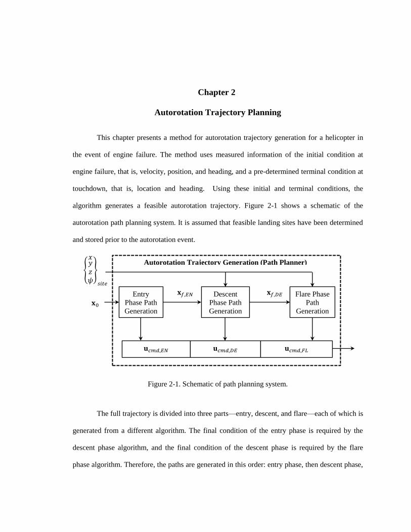
This chapter presents a method for autorotation trajectory generation for a helicopter in
the event of engine failure. The method uses measured information of the initial condition at
engine failure, that is, velocity, position, and heading, and a pre-determined terminal condition at
touchdown, that is, location and heading. Using these initial and terminal conditions, the
algorithm generates a feasible autorotation trajectory. Figure 2-1 shows a schematic of the
autorotation path planning system. It is assumed that feasible landing sites have been determined
and stored prior to the autorotation event.
Figure 2-1. Schematic of path planning system.
The full trajectory is divided into three parts—entry, descent, and flare—each of which is
generated from a different algorithm. The final condition of the entry phase is required by the
descent phase algorithm, and the final condition of the descent phase is required by the flare
phase algorithm. Therefore, the paths are generated in this order: entry phase, then descent phase,
𝐱𝑓 𝐸𝑁
𝑥𝑦𝑧𝜓
𝑠𝑖𝑡𝑒
𝐱
Entry
Phase Path
Generation
Descent
Phase Path
Generation
Flare Phase
Path
Generation
𝐮𝑐𝑚𝑑 𝐸𝑁 𝐮𝑐𝑚𝑑 𝐷𝐸 𝐮𝑐𝑚𝑑 𝐹𝐿
𝐱𝑓 𝐷𝐸
Autorotation Trajectory Generation (Path Planner)
23
and then flare phase. The terminal condition of the descent phase is based on a pre-calculated safe
landing set [11, 12]. The path-generating algorithm for each autorotation phase uses a simplified
rotorcraft model to represent the aircraft dynamics.
While the methods are general to all rotorcraft, a full-scale generic utility helicopter is
selected as a demonstration helicopter to illustrate results from the developed algorithms. The
properties of the helicopter (Table 2-1) are used to specify criteria in the algorithm throughout
this chapter. Examples of trajectory solutions shown in this chapter are determined specifically
for the helicopter.
2.1 Specifications of Generic Utility Helicopter
In this dissertation, a non-linear FLIGHTLAB simulation model of a generic utility
helicopter is used to evaluate the performance of the trajectory-generating algorithm. The
structures and aerodynamic surfaces in the FLIGHTLAB model of the generic utility helicopter
are similar to those of an UH-60 Blackhawk helicopter. The FLIGHTLAB rotorcraft model is a
bare-airframe helicopter model with an engine model. Without closed-loop controls, the bare-
airframe model comprises the dynamics and aerodynamics response characteristics of the
fuselage, the main rotor, the tail rotor, and the vertical and horizontal stabilizers. The engine
model allows RPM variation due to the time lag response of engine power; no engine governor is
included. Model inputs are main rotor collective blade pitch angle, lateral cyclic pitch angle,
longitudinal cyclic pitch angle and tail rotor collective blade pitch angle (in radians). An actuator
model is included to represent the time lag of control surface due to mechanical hardware. A first-
order actuator model with time constant of 0.02 is used in each control surface. The key
properties of this generic utility helicopter model are shown in Table 2-1. Note that the control

24
surface range of the tail rotor is extended from the normal range in order to allow a sufficient
control for the turns in autorotation flights.
Table 2-1. Properties of generic utility helicopter
Description Value
Aircraft
Design gross weight (lbf)
Maximum gross weight (lbf) [88]
16285.1
20250.0
Main rotor: Articulated rotor
number of blades
nominal speed (rad/s)
radius (ft)
blade weight (lbf)
polar moment of inertia (sl-ft2)
built-in tilt (deg)
4
27
26.83
283.56050
6052
3 (forward)
Tail rotor:
number of blades
nominal speed (rad/s)
radius (ft)
4
124.62
5.5
Control surface range: [min, max]
main rotor lateral cyclic (deg)
main rotor longitudinal cyclic (deg)
main rotor collective (deg)
tail rotor collective (deg)
[-8, 8]
[-12.5, 16.3]
[5.0, 25.9]
[0.0, 36.5]

25
Figure 2-2. Principal dimensions of the generic utility helicopter (similar to UH-60) [88]
The principal dimensions of the helicopter are illustrated in Figure 2-2. The center of
gravity (CG) of the rotorcraft simulation model locates at 5 ft behind, 7 ft above and between the
two main landing gears. In the present work, the rotorcraft position is referred to this CG point.
The computation of autorotation trajectories is based on this CG location. The touchdown point in
trajectory is 7 ft above the ground.
2.2 Vehicle Dynamics for Trajectory Computation
To represent the rotorcraft dynamics in a computationally efficient way, a point mass
model is used. The model has seven states: three of which are represented by the three-
dimensional position vector, and the others are horizontal speed, descent rate, rotor speed, and
heading:
[ ] (2.1)

26
The control inputs for the model are the rotor orientation (roll and pitch attitude) and the
thrust coefficient, which define thrust orientation and magnitude, respectively:
[ ] (2.2)
The simplified model of the vehicle dynamics includes the following assumptions:
1) The orientation of the rotor tip path plane defined by the roll and pitch attitudes,
and , are not substantially different from the vehicle orientation, and , in
quasi-steady flight.
2) The change in rotor thrust is achieved instantaneously.
3) The aircraft is always in zero sideslip coordinated flight, where the heading is
aligned with the flight path, .
4) The atmospheric conditions are assumed to be constant.
With these assumptions, the equations of motion can be derived as:
(2.3)
(2.4)
(2.5)
⁄ (2.6)
(2.7)
(2.8)
(2.9)
The power coefficient, , is defined as
(2.10)
where is an advance ratio and is an inflow ratio defined, respectively, as follows:
⁄ (2.11)

27
[ ] ⁄ (2.12)
The advance velocity, , is a velocity component parallel to the rotor tip path plane. It is
computed by
√
(2.13)
The induced velocity, , is approximated by
(2.14)
where is an induced power correction factor, is a factor accounting for any decrease in
the induced velocity due to the ground effect, and and are the ideal induced velocity in
hover and a ratio of the actual induced velocity to the ideal induced velocity in hover,
respectively.
The ideal induced velocity, , and the ratio, , are defined, respectively, as
√ ⁄ (2.15)
√(
)
(2.16)
where and are defined, respectively, as:
⁄ (2.17)
⁄ (2.18)
In this point mass model, helicopter dynamics are defined in the aircraft local coordinate
frame, which is an aircraft-carried Cartesian coordinate system with x- and y-axes, and , in
the horizontal plane and z-axes, , pointing downward. Figure 2-3 shows the definition of the
parameters described in the equations of motion. The orientation of the rotor tip path plane is
represented by the body coordinate system such that the x- and y-axes, and , are in the plane
of the rotor tip path and indicate the front and starboard side, respectively. The bank and pitch
angles, which define the orientation of the rotor tip path plane, are Euler angles that describe the

28
body coordinate system with respect to the local coordinate system. Figure 2-4 illustrates the
definitions of the aircraft bank and pitch angles.
Figure 2-3. Definitions of the coordinates and key parameters of the helicopter point mass model.
Figure 2-4. Definitions of the aircraft pitch and bank angles.
The aircraft position is defined by the inertial North-East-Down coordinate system (Earth
reference frame). Figure 2-5 illustrates the definitions of the aircraft position and heading in the
inertial system.
𝑇 𝐶𝑇
𝜇
𝜆 𝑉
𝛼
𝜃
𝑊 𝑚𝑔
𝑥𝑙 (Forward, horizontal)
��𝑙 (Vertical)
𝑥𝑙
��𝑙
��𝑙
𝑥𝑙
𝑥𝑏
��𝑙
��𝑙
𝜃
��𝑙
𝑥𝑏
��𝑏
��𝑏
𝜙

29
Figure 2-5. Definitions of the aircraft position and heading, .
2.3 Entry Phase Path Generation
The objective of the entry phase path is to initiate the autorotation descent after engine
failure and recover the rotor speed while the descent phase path solution is being computed. The
entry phase time duration, , depends on the performance of the onboard computer and is
predetermined prior to the flights. The entry phase is designed to be a fixed-time duration
maneuver in which the rotorcraft holds constant heading and attempts to recover rotor speed in
order to enter a steady descent condition. The entry phase trajectory problem is formulated as a
trajectory optimization problem with no terminal constraints. The control inputs during the flight
are the parameters in the optimization method and are solved to satisfy the dynamics and
limitations of the rotorcraft.
𝑇𝑜𝑝 𝑣𝑖𝑒𝑤
𝑥 (North)
�� (East)
𝜓
𝑥
𝑥𝑙
��𝑙
Aircraft
Position

30
In this section, two optimization methods are developed to compute the entry phase
trajectories. Both methods discretize the entry phase flight into small time intervals and take the
control inputs at each time interval as parameters to optimize. However, the first method is
formulated to find a set of command inputs for the whole entry phase flight that results in an
optimum response, whereas the second method aims to find the optimal command inputs for each
time interval.
2.3.1 Entry Path Optimization Method 1
In the first method, the cost function is formulated to minimize the control effort
(changes in thrust and pitch attitude) and the rotor speed drop during the entry phase and to
minimize the altitude loss at the end of the entry phase. The aircraft flight dynamics are
incorporated using Euler integration of the point mass model
(2.19)
where is computed by using the point mass model.
The parameter-optimization problem can be written for N intervals as
Minimize ({ }) { }
{
}
(2.20)
subject to
(2.21)
(2.22)
(2.23)

31
where represents the helicopter dynamics, { }, is a nominal rotor
speed, and
The cost functions corresponding to control effort, rotor speed drop, and altitude loss in
the optimization problem are
∑( )
(2.24)
∑ (2.25)
∑ (2.26)
(2.27)
(2.28)
where 1, 2, …, N.
To improve computational tractability, the trajectory is found by parameterizing inputs
and using a cubic spline. The dimension of the parameter-optimization problem is reduced
by discretizing the flight with a big time interval (small number of nodes) and using a cubic
spline fit to generate control inputs during the interval between the nodes:
{ } { } (2.29)
where is a cubic spline fit function, N is the number of nodes corresponding to the time step
that the simulation runs to generate the trajectory, K is the number of nodes that the entry phase

32
flight is discretized to represent as parameters in the optimization method, and
Figure 2-6. Example of entry path input solution for 100 knots airspeed from the first method,
sec, N = 400 nodes, and K = 9 nodes.
Figure 2-6 shows an example of the entry path input solution for an initial airspeed of 100
knots and a time duration of four seconds. In this example, the four-second path is divided into
eight intervals (nine nodes). The smaller time step that the simulation runs is 0.01 seconds.
The weight values selected for the cost functions can significantly affect the path solution
results. Whereas the weights for the final conditions (altitude loss and final rotor speed) are given
in order to obtain the path solution with a final condition close to the desired conditions, the
weights for the control effort and the drop in rotor speed during the flight are given to prevent
abrupt maneuvers from the solution. It was found that the following weights give reasonable
results for the specified time step of 0.01 seconds and a nominal rotor speed of 27 rad/s:
0 0.5 1 1.5 2 2.5 3 3.5 4-10
0
10
R (
deg)
0 0.5 1 1.5 2 2.5 3 3.5 44
6
8x 10
-3
CT
0 0.5 1 1.5 2 2.5 3 3.5 425
26
27
(
rad/s
)
Time (s)

33
{ } {
} (2.30)
2.3.2 Entry Path Optimization Method 2
For the second method, the control inputs are optimized at each time step of the
maneuver rather than over the entire trajectory. The control input solution for the current time
node is used to compute the vehicle condition for the next time node by using Euler integration of
the point mass model, as shown in Eq. (2.19). The complete entry phase is computed by repeating
this process of finding the control input solution and updating the vehicle condition for all the
discretized time nodes. Figure 2-7 illustrates the algorithm process for this method. The flight
condition is divided into two categories by using horizontal velocity. Two different objective
optimization functions are formulated, one for each of the two flight condition categories. If the
horizontal velocity is lower than the operating velocity for the descent phase, , the objective
function to recover rotor speed and increase horizontal speed is implemented. On the other hand,
if the horizontal velocity is higher than the operating velocity, , the objective function for
pure rotor speed recovery is used.

34
Figure 2-7. Optimization process for entry path method 2.
In order to “recover the rotor RPM by using airspeed,” the cost function is formulated to
minimize the rotor speed drop and the horizontal airspeed deceleration for the vehicle condition at
the current time step. The parameter-optimization problem for the time node can be written as
Minimize (2.31)
subject to
{
} (2.32)
(2.33)
where represents the helicopter dynamics, { }, is the maximum
allowed change of the control inputs, and is an additional cost function which penalize
rotor speed higher than the nominal rotor speed.
Recover Rotor RPM
by Using Airspeed
Update Vehicle
Condition
𝑢𝑙 < 𝑢𝑙 𝑚𝑖𝑛
Recover Rotor RPM
and Increase
Horizontal Speed
Initial Vehicle
Condition
No
Yes
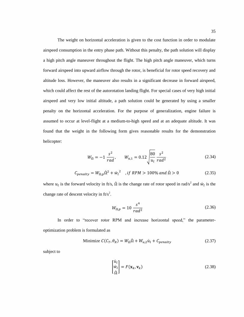
35
The weight on horizontal acceleration is given to the cost function in order to modulate
airspeed consumption in the entry phase path. Without this penalty, the path solution will display
a high pitch angle maneuver throughout the flight. The high pitch angle maneuver, which turns
forward airspeed into upward airflow through the rotor, is beneficial for rotor speed recovery and
altitude loss. However, the maneuver also results in a significant decrease in forward airspeed,
which could affect the rest of the autorotation landing flight. For special cases of very high initial
airspeed and very low initial altitude, a path solution could be generated by using a smaller
penalty on the horizontal acceleration. For the purpose of generalization, engine failure is
assumed to occur at level-flight at a medium-to-high speed and at an adequate altitude. It was
found that the weight in the following form gives reasonable results for the demonstration
helicopter:
√
(2.34)
(2.35)
where is the forward velocity in ft/s, is the change rate of rotor speed in rad/s2 and is the
change rate of descent velocity in ft/s2.
(2.36)
In order to “recover rotor RPM and increase horizontal speed,” the parameter-
optimization problem is formulated as
Minimize (2.37)
subject to
[
] (2.38)

36
(2.39)
It was found that the weight in the following form gives reasonable results:
(2.40)
(2.41)
Figure 2-8. Example of an entry path input solution for 100 knots airspeed from the second
method.
Figure 2-8 shows an example of an entry path input solution for an initial airspeed of 100
knots and a time duration of four seconds from the second entry phase optimization method. In
this result, the optimum input solution is found for every time step that the simulation runs (0.01
seconds).
For an initial airspeed below the criterion, , the entry phase path requires more time
to recover rotor speed and increase airspeed. Figure 2-9 shows an example entry path input
0 0.5 1 1.5 2 2.5 3 3.5 4-10
0
10
R (
deg)
0 0.5 1 1.5 2 2.5 3 3.5 40
0.005
0.01
CT
0 0.5 1 1.5 2 2.5 3 3.5 425
26
27
(
rad/s
)
Time (s)

37
solution for the initial hover case from the second entry phase optimization method. The solution
requires approximately nine seconds to recover horizontal velocity. In this result, the optimum
input solution is found for every time step that the simulation runs (0.01 seconds).
Figure 2-9. Example of an entry path input solution from the second method for the initial hover
case.
0 1 2 3 4 5 6 7 8 9-50
0
50
R (
deg)
0 1 2 3 4 5 6 7 8 90
0.005
0.01
CT
0 1 2 3 4 5 6 7 8 90
50
100
ul (
ft/s
)
0 1 2 3 4 5 6 7 8 90
50
wl (
ft/s
)
0 1 2 3 4 5 6 7 8 924
26
28
(
rad/s
)
Time (s)

38
2.3.3 Analysis of Entry Phase Trajectory Methods
The two optimization methods presented previously are capable of finding entry phase
trajectory solutions for several initial conditions. Figure 2-10 shows four-second entry path
solutions for several initial level-flight airspeeds from the two methods. Both methods use a fair
amount of time in the computation. Due to these required computation times, the two methods are
hardly able to update the entry trajectory in real-time.
In order to have the entry phase trajectory suitable for the initial condition in real-time
flights, a set of trajectory solutions that covers a wide range of possible initial conditions must be
pre-generated and stored. In the event of engine failure, the entry path is properly chosen from
this set of pre-computed trajectory solutions for the current flight condition. Such a set that
contains all entry path solutions would require a fair amount of memory in data storage.
Consider the trajectory commands of entry path solutions shown in the top and middle
plots in Figure 2-10. The trajectory commands for different initial conditions from the second
method display more consistency in terms of the shape and only differ in terms of magnitude.
Therefore, the trajectory solution for the initial airspeed of 170 ft/s can be fairly approximated by
linearly interpolating between those of the lower and upper initial airspeeds of 90 ft/s and 240
ft/s. Such an interpolation would reduce the number of entry path solutions required in the
storage. The entry path solution can be pre-computed for some representative initial conditions
and the entry path solution that is suitable for the initial condition at engine failure can be
generated by using an interpolation of representative trajectory solutions.

39
Figure 2-10. Comparison of path solutions from the two optimization methods.
0 1 2 3 4-8
-4
0a x
(ft
/s2)
0 1 2 3 40
200
400
600
800
1000
x (
ft)
0 1 2 3 424
26
28
(
rad/s
)
Time (s)
0 1 2 3 4-10
0
10
20
30
40
a z (f
t/s2
)
0 1 2 3 40
10
20
30
40
w (
ft/s
)
Time (s)
0 1 2 3 40
20
40
60
80
100z
(ft)
90 ft/s (Mthd1)
170 ft/s (Mthd1)
240 ft/s (Mthd1)
90 ft/s (Mthd2)
170 ft/s (Mthd2)
240 ft/s (Mthd2)

40
2.4 Descent Phase Path Generation
The descent phase path generation is designed to find a feasible three-dimensional
trajectory from the point of engine failure to the point at which the rotorcraft can safely perform
an autorotative flare landing to a desired touchdown location. The initial state of the path,
{ }
, and the desired final state, { } , are the initial
and terminal constraints of the trajectory problem. The desired trajectory is defined as a set of
aircraft states that satisfies the aircraft autorotation dynamics and in which the initial states and
the desired destination states are members. The desired trajectory can be written as
|
( )
( )
(2.42)
where represent the aircraft dynamics and is the control input to the aircraft.
The controls and some of the states will also have constraints due to physical and/or
operational limits on the aircraft (e.g., the maximum airspeed limit in the autorotation procedure
[88]):
(2.43)
(2.44)
The descent phase flight is assumed to be out of ground effect (the flight is not at a very
low altitude). The ground-effect factor is neglected in the computation of the descent phase
trajectory solutions.
2.4.1 Trajectory Formulation
An aircraft trajectory in three-dimensional space can be determined by planning a
trajectory in two dimensions on a horizontal north-east plane and extending that trajectory to

41
three dimensions by adding either a corresponding vertical flight path angle or a descent rate. In
this descent phase trajectory planning problem, both the allowable flight path angle and the
descent rate in autorotation are highly constrained and vary with airspeed, bank angle (rate of
turn), rate of acceleration/deceleration, and rotor speed. Also, the aircraft must change its velocity
during the course of the maneuver to achieve the desired airspeed and rotor speed. The classic
Dubins’ concept, which is used to find an optimal path between two planar points with initial and
terminal constraints in heading for an aircraft with a constant speed and bounded bank angle, is
adopted and modified by incorporating three additional parameters. First, constant acceleration is
allowed in addition to the standard turn-straight-turn parameterization. Second, the descent rate is
explicitly modeled to permit three-dimension trajectories. Third, the constraint on the rate of the
bank angle change is applied to account for the roll attitude dynamics in the transition between
each segment. The vertical trajectory is decoupled from the trajectory in the horizontal plane and
can be obtained from the simplified rotorcraft model after the path in the horizontal plane is
found. The trajectory in horizontal plane is a three-segment, turn-straight-turn path which the
aircraft uses different bank angle and constant acceleration/deceleration along the segments.
Additional acceleration allows the aircraft to attain the desired velocity at its destination. The
constant bank angle, acceleration, and time duration in each segment are considered to be the
parameters that define the planar path. The set of planar-path-defining parameters with non-zero
bank angles is unique for a specified path. The autorotation trajectory problem in the horizontal
plane is converted into a parameter-optimization problem to find a set of planar-path-defining
parameters that satisfies Eqs. (2.42)–(2.44).
[ ]
(2.45)
where the subscripts 1, 2, and 3 identify the first turn, the straight flight, and the second turn
segments, respectively.

42
These modified Dubins curves use the same concept as the Dubins’ Right-turn-Straight-
Right-turn (RSR), Left-turn-Straight-Left-turn (LSL), Right-turn-Straight-Left-turn (RSL), and
Left-turn-Straight-Right-turn (LSR), in all of which the aircraft is allowed to turn more than 360º
(that is, through multiple turns). Transitions between the flight conditions, straight flight and turn,
occur at the beginning and end of each turning segment (as illustrated in Figure 2-11). During
these transitions, not only does velocity vary with constant acceleration, but the aircraft bank
angle varies with limited rate as well. In the transition, the aircraft makes a curve that is different
from the turning curve of a constant bank angle in the middle of the segment. With a constant
bank angle and varied velocity, the middle of turning segments make a spiral curve in the
horizontal plane, in which the turning radius varies and the closed-form expressions for this spiral
curve can be derived analytically.
Figure 2-11. Turning segment in the modified Dupins’ paths.
Initial Straight Flight
Return to
Straight Flight
Turn with Constant
Bank Angle
(Varied Airspeed)
Transition to
Straight Flight
(Varied Bank Angle
and Airspeed)
Transition to
Constant Bank Angle Turn
(Varied Bank Angle and
Airspeed)
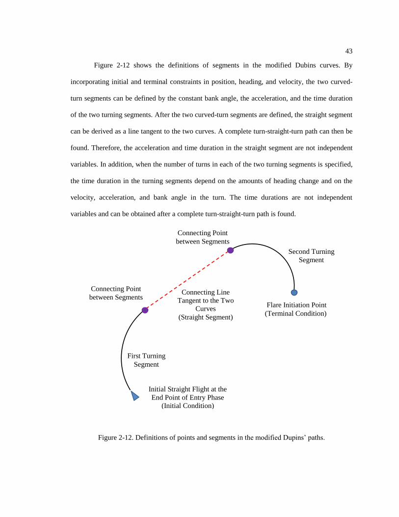
43
Figure 2-12 shows the definitions of segments in the modified Dubins curves. By
incorporating initial and terminal constraints in position, heading, and velocity, the two curved-
turn segments can be defined by the constant bank angle, the acceleration, and the time duration
of the two turning segments. After the two curved-turn segments are defined, the straight segment
can be derived as a line tangent to the two curves. A complete turn-straight-turn path can then be
found. Therefore, the acceleration and time duration in the straight segment are not independent
variables. In addition, when the number of turns in each of the two turning segments is specified,
the time duration in the turning segments depend on the amounts of heading change and on the
velocity, acceleration, and bank angle in the turn. The time durations are not independent
variables and can be obtained after a complete turn-straight-turn path is found.
Figure 2-12. Definitions of points and segments in the modified Dupins’ paths.
Initial Straight Flight at the
End Point of Entry Phase
(Initial Condition)
First Turning
Segment
Second Turning
Segment
Flare Initiation Point
(Terminal Condition)
Connecting Line
Tangent to the Two
Curves
(Straight Segment)
Connecting Point
between Segments
Connecting Point
between Segments

44
The dimension of the parameter-optimization problem can be significantly reduced by
finding dependent variables analytically. All dependent variables are derived in order to provide a
computationally efficient solution that automatically meets the initial and terminal constraints on
the position in the horizontal plane, the heading, and the horizontal velocity. A geometry-based
searching algorithm is developed to find dependent variables for a given set of independent
variables and the initial and terminal trajectory constraints. The searching algorithm is an iterative
trial-and-error method combining three different searching methods. The autorotation trajectory
problem is now a problem of finding a set of independent variables that creates a horizontal path
for which the corresponding vertical trajectory satisfies the constraint described in Eqs. (2.42)–
(2.44):
[ ]
(2.46)
The modified three-dimensional Dubins curve is extended from the two-dimensional
acceleration path by adding the decrease in altitude that occurs over the path in autorotation
descent. The simplified rotorcraft model can be used to determine the vertical velocity in quasi-
steady state autorotation at all points along the path. In addition to the parameters that define the
planar path, the rotor speed provides an additional parameter that can be used to control the rate
of descent. The autorotation trajectory planning problem can now be treated as a problem of
finding seven parametric control variables:
[ ]
(2.47)
The process of generating a descent phase trajectory is illustrated in Figure 2-13. The
modified Dubins curve in three-dimensional space is illustrated in Figure 2-14. The three
segments consist of a turn, a straight segment, and a turn, with the aircraft descending in
autorotation along all three segments. The descent rates at any instant along the flight path are
obtained from a mapping of quasi–steady state power-off autorotation condition.

45
Figure 2-13. Descent phase autorotation trajectory generating process.
No
𝐱𝐷𝐸 [𝑥 𝑦 𝑧 𝑢𝑙 𝜓 𝑥d 𝑦d 𝑧d 𝑢𝑙 𝑑 𝜓d]𝑇
Initial and Terminal Constraints
Search for Straight Segment
𝑡 𝑃 𝑎𝑥 𝑙 𝜙 𝑎𝑥 𝑙 𝜙 𝐱𝐷𝐸 )
𝑧 𝑡𝑑 𝐻 Ω Ω Ω 𝐱𝐷𝐸 𝐮 Quasi-steady Autorotation
𝐮 [𝑎𝑥 𝑙 𝜙 Ω Ω 𝑎𝑥 𝑙 𝜙 Ω ]𝑇
Optimize
Optimal 𝐮?
Trajectory Solution
Yes
No
Select Path Type:
RSR, RSL, LSR, LSL
Optimizer
Planar
Path
Planning
Valid 𝐮 𝑡 ?
Yes

46
Figure 2-14. Example of descent phase autorotation trajectory.
2.4.2 Planar Path Planning
The modified Dubins curve is derived from the equations of motion. The trajectory
defined in Equation (2.42) can be calculated by the following integration:
∫
∫
(2.48)
where is the time duration of the segment.
-1000
0
1000
2000
3000
4000
5000
-1000
0
1000
2000
3000
4000
5000
0
500
1000
1500
2000
East location (ft)
North location (ft)
Heig
ht (f
t)
Segment 1
Segment 2
Segment 3
Landing Site
Target Destination
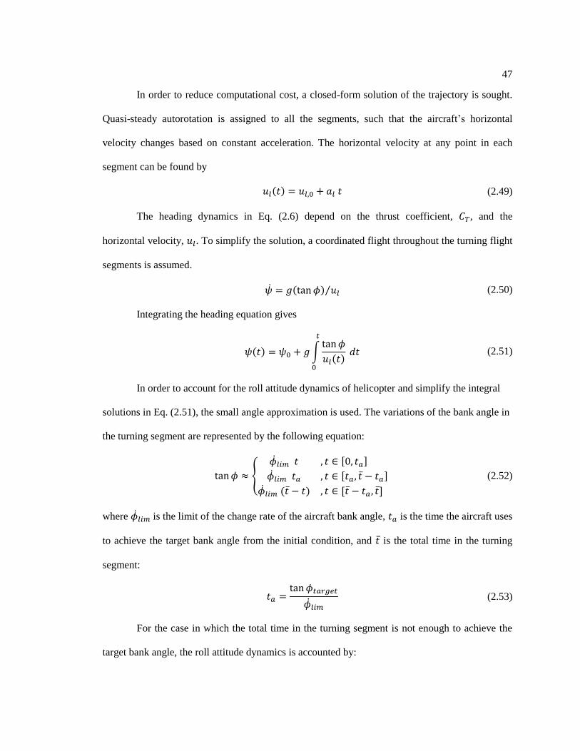
47
In order to reduce computational cost, a closed-form solution of the trajectory is sought.
Quasi-steady autorotation is assigned to all the segments, such that the aircraft’s horizontal
velocity changes based on constant acceleration. The horizontal velocity at any point in each
segment can be found by
(2.49)
The heading dynamics in Eq. (2.6) depend on the thrust coefficient, , and the
horizontal velocity, . To simplify the solution, a coordinated flight throughout the turning flight
segments is assumed.
⁄ (2.50)
Integrating the heading equation gives
∫
(2.51)
In order to account for the roll attitude dynamics of helicopter and simplify the integral
solutions in Eq. (2.51), the small angle approximation is used. The variations of the bank angle in
the turning segment are represented by the following equation:
[ ]
[ ]
[ ]
(2.52)
where is the limit of the change rate of the aircraft bank angle, is the time the aircraft uses
to achieve the target bank angle from the initial condition, and is the total time in the turning
segment:
(2.53)
For the case in which the total time in the turning segment is not enough to achieve the
target bank angle, the roll attitude dynamics is accounted by:

48
{
[ ]
[ ] (2.54)
Figure 2-15 shows the time histories of the functions that account for varied bank angle
in the turning segment. In the first case (the upper figure), the total time in the turning segment is
enough for the rotorcraft to achieve the target bank angle and return to a level flight at the end of
the segment. In the second case (the lower figure), the time required to achieve target bank angle
and return to a level flight is more than the time in turning segment. The bank angle must be
decreased before it reaches the target bank angle in order to have zero bank angle at the end of
turning segment.
Figure 2-15. Definitions of the case with achieved bank angle (upper) and the case with
insufficient time (lower).
𝑡 𝑡 𝑡𝑎 𝑡𝑎
𝜙𝑡𝑎𝑟𝑔𝑒𝑡
𝐹 𝑡 𝜙
𝑡
𝑡 𝑡 /2
𝜙𝑡𝑎𝑟𝑔𝑒𝑡
𝐹 𝑡 𝜙
𝑡
𝑑𝐹
𝑑𝑡 ��𝑙𝑖𝑚, 0, ��𝑙𝑖𝑚
𝑑𝐹
𝑑𝑡 ��𝑙𝑖𝑚, ��𝑙𝑖𝑚

49
2.4.2.1 Closed-form Solution
In this section closed-form solutions of position and heading in the turning curves are
derived in order to provide computational efficiency for the searching algorithm. A closed-form
solution of heading dynamics in Eq. (2.51) can be obtained analytically. However, the analytical
solutions are in a different form for the acceleration/deceleration turns and the constant velocity
turns. For the acceleration/deceleration turns, the solution of the heading motion can be obtained
as
{
(
) [ ]
(
) [ ]
(
) [ ]
(2.55)
where
(
) (2.56)
(
)
(2.57)
The final heading of the turning segment is defined by:
(
)
(
)
(
)
(2.58)
For the case in which the target bank angle is not achieved, Eq. (2.55) can be reduced.
The solution of the heading motion, thus, becomes:

50
{
(
) [ ]
(
) [ ]
(2.59)
where
(
) (2.60)
For this case, the final heading is defined by:
(
)
(
)
(2.61)
For constant velocity turns, the solution of the heading dynamics is
{
[ ]
[ ]
(
) [ ]
(2.62)
The solution of the heading dynamics in Eq. (2.62) can be reduced for the case in which
the target bank angle is not achieved:
{
[ ]
[ ]
(2.63)
For the aircraft position, the equation of the aircraft’s horizontal motion in the presence
of wind in Eqs. (2.7) and (2.8) can be presented as
∫
(2.64)

51
∫
(2.65)
A closed-form solution of the aircraft position is sought by substituting Eqs. (2.49),
(2.55), (2.59), (2.62), and (2.63) into Eqs. (2.64) and (2.65). Analytical solutions are found only
for the region of the constant bank angle, but they can be used in both the
acceleration/deceleration turn and the constant speed turn. The equation substitution gives
∫( ) (
(
))
(2.66)
∫( ) (
(
))
(2.67)
Closed-form solutions of Eqs. (2.66) and (2.67) can be written as:
[( )
{ }
( ) { }] {
}
(2.68)
[( )
{ }
( ) { }] {
}
(2.69)
where , are horizontal velocity and heading at time as computed by Eqs. (2.49) and
(2.55) (or (2.62) if the velocity is constant in the turn).
2.4.2.2 Finding the Straight Segment
The initial and final states, as defined in Eq. (2.42), are specified given the rotorcraft’s
position, heading, and velocity at the end of the entry phase and the beginning of the flare phase

52
at a pre-defined landing site. If the time duration in the first segment and the independent
variables in Eq. (2.46) are specified, the heading in the straight segment can be found by the
equation of the heading motion:
( ) (2.70)
where is the aircraft heading in the straight segment.
The time duration in the third segment depends on the geometry of the path and can be
found from the headings in the straight segment and at the destination:
(2.71)
where is an inversion function of the heading motion and is the number of turns.
With the time durations in the turning segments, and , the two turning segments can
be obtained from the independent variables and the path initial and terminal constraints. The
acceleration and time duration in the straight segment can then be derived from the velocities and
positions at the end of first segment, { } and at the beginning of the third segment,
{ }. By projecting the vector from the end of the first segment to the beginning of the
third segment, , into the direction of the aircraft heading, , a distance in which the aircraft has
to change velocity from velocity at the end of first segment, , to velocity at the beginning of
third segment, , is obtained. The definition of parameters is illustrated in Figure 2-16. With the
distance and velocity boundary, the required constant acceleration can be found as
{
(2.72)
Note that the wind velocity is assumed to be lower than the aircraft’s airspeed. A negative
number from the projection implies an impossible path for the given first segment time duration.
For this case, no second segment is given for the path. This modified Dubins curve has only two

53
turning segments. The factor is used to allow a small deviation in horizontal velocity at the
connecting point in this case.
Then, the time duration in the second segment can be derived:
{
(2.73)
Figure 2-16. Definitions of the parameters in the geometry-based search method.
2.4.2.3 Finding Dependent Variables for Planar Path
The previous section has presented that, by giving the time duration in the first segment,
the other dependent variables can be derived for the set of independent variables and the path
constraints. However, the time duration is not yet known. This section present an iterative method
𝜓
North 𝑥𝑙
��𝑙
�� [𝑥 𝑦 ]
��
�� [𝑥 𝑦 ]
𝑟 𝑢
𝑢
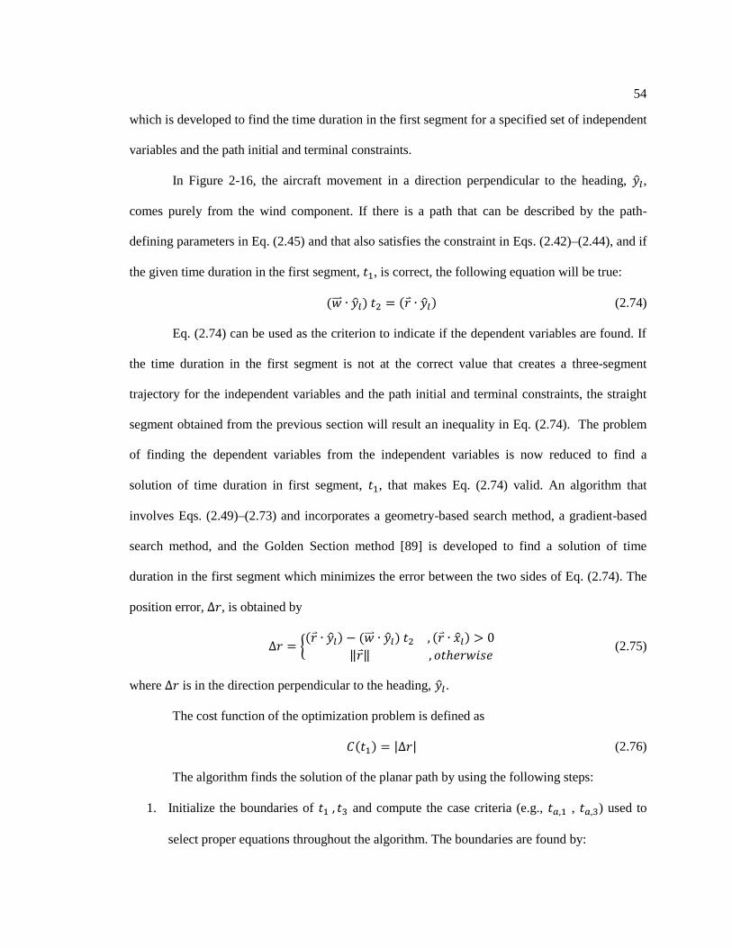
54
which is developed to find the time duration in the first segment for a specified set of independent
variables and the path initial and terminal constraints.
In Figure 2-16, the aircraft movement in a direction perpendicular to the heading, ,
comes purely from the wind component. If there is a path that can be described by the path-
defining parameters in Eq. (2.45) and that also satisfies the constraint in Eqs. (2.42)–(2.44), and if
the given time duration in the first segment, , is correct, the following equation will be true:
(2.74)
Eq. (2.74) can be used as the criterion to indicate if the dependent variables are found. If
the time duration in the first segment is not at the correct value that creates a three-segment
trajectory for the independent variables and the path initial and terminal constraints, the straight
segment obtained from the previous section will result an inequality in Eq. (2.74). The problem
of finding the dependent variables from the independent variables is now reduced to find a
solution of time duration in first segment, , that makes Eq. (2.74) valid. An algorithm that
involves Eqs. (2.49)–(2.73) and incorporates a geometry-based search method, a gradient-based
search method, and the Golden Section method [89] is developed to find a solution of time
duration in the first segment which minimizes the error between the two sides of Eq. (2.74). The
position error, , is obtained by
{
‖ ‖ (2.75)
where is in the direction perpendicular to the heading, .
The cost function of the optimization problem is defined as
| | (2.76)
The algorithm finds the solution of the planar path by using the following steps:
1. Initialize the boundaries of and compute the case criteria (e.g., , ) used to
select proper equations throughout the algorithm. The boundaries are found by:

55
(2.77)
(2.78)
2. Suggest , [ ]
3. Evaluate the cost:
3.1. Define the planar path.
3.1.1. Compute and
3.1.2. Find [ ]
3.1.3. Compute and
3.1.4. Find the straight segment, ,
3.2. Compute the cost function
4. Sort the trials and errors via the three-point pattern (using the bracketing algorithm) [89].
5. Check that the stopping criteria have been met. If it is true, return the data corresponding
to the smallest cost value. Else, repeat the process beginning at Step 2.
2.4.2.4 Searching for Solution
The solution of the time duration in the first turning segment is sought by three search
methods: (1) a geometry-based search method, (2) a gradient method (steepest descent), and (3)
the Golden Section method. The geometry-based search method relies on the confidence that a
planar path solution exists. The method suggests a new trial of for the next iteration by
estimating a correct heading based on the geometric error of the previous trial (as illustrated in
Figure 2-17).

56
Figure 2-17. Geometry-based search method.
The next trial is obtained by
(2.79)
(2.80)
where the subscript, , indicates the iteration number and
(2.81)
[
( )
( )
] (2.82)
The gradient-based search method also relies on the confidence that a planar path
solution exists as the geometry-based method. The method computes a new trial based on
previous trials and errors at a minimum recorded point and its next intermediate point. This
method is utilized in some cases in which the geometry-based search method is not effective
(| | < ). A new gradient-based trial is estimated by
(
( ) ) (2.83)
Δ𝜓
�� 𝜓
North 𝑥𝑙
��𝑙
��
��
��
𝑟 𝑢
Δ𝑟
�� 𝜓
North 𝑥𝑙
��𝑙
��
��
��
𝑟
𝑢
Δ𝜓
Δ𝑟 <

57
where is the minimum input and is the next intermediate point of in the
input domain.
The Golden Section method [89] is a popular uniform reduction strategy that reduces the
interval of uncertainty to 61.8% for every trial. The method is capable of finding an optimal
solution which minimizes the position error at the destination when an exact solution of planar
path does not exist. This method is utilized in cases where (1) a planar path solution may not
exist, (2) the three-point pattern is formed and the other methods are not effective. The uncertain
range is obtained from recorded data of previous trials.
The follow list is used to indicate the uncertain range:
1. A difference in the sign of . If , , and
( ( )) ( ( )), then the uncertain range is [ ].
2. The edge of the three-point pattern ([ ] in Figure 2-18). If a three-point pattern is
found in the previous trials.
3. If none of the above exists, the uncertain range is [ ].
The method selected for use in each iteration is based on the confidence that the planar
path solution exists ( [ ] ) and on the efficiency of each
method. The geometry-based method is very effective for the case in which the planar path
solution exists. The geometry-based method is selected for the first number of iterations. During
these iterations, the suggested trial is observed: (1) if the suggested trail is too close to the
previous trial | | < , the gradient-based method is used; (2) if the suggested trail
has not converged to any point, the Golden Section search method is used instead.

58
2.4.2.5 Planar Path Computation
In this step, the two turning segments corresponding to the new prediction of the time
duration, , are defined. From the initial aircraft states and the time duration trial, the position,
velocity and heading at the end of the first turning segment are computed. The time duration in
the second turning segment, , is found from the change in heading from the end of first
segment to the desired heading at the destination. The position, velocity, and heading at the
beginning of the second turning segment are then computed from the desired aircraft states at the
destination and the computed time duration. Finally, the straight segment is derived, and the cost
function of the planar path optimization problem (Eq. (2.76)) is evaluated.
In the process undertaken to compute the two turning segments, each turning curve is
identified as belonging to one of four types of turns: the constant speed, transition curve; the
constant speed, combined steady curve; the accelerating, transition curve; and the accelerating,
combined quasi-steady curve. The time duration and the heading change in each turning curve
can be used to determine the type of turn for each turning segment. In the case for which the
turning time duration is not available, the heading change in the turning curve is used in the
identification instead. The heading change is found by
{
(2.84)
where
[ ] (2.85)
The criteria, and , are used to determine whether the curve of the turning segment
is composed of two transition (varying bank angle) curves with a quasi-steady region in the
middle (case 1: or ) or of two consecutive transition curves (case 2:
or ). The planar path parameters, and , are used to determine

59
whether the segment is an accelerating curve or a constant speed curve. Table 2-2 shows the
summary of the turning curve categories.
Table 2-2. Turning segment categorization
Criteria
{ }
{ }
Case A :
constant speed, transition curve
Case B :
constant speed, combined steady
curve
Case C :
accelerating, transition curve
Case D :
accelerating, combined quasi-
steady curve
The aircraft states in the transition region are computed by using numerical integration. A
trapezoidal integration is chosen with a specified time step to maintain acceptable computational
accuracy and speed. For the steady and quasi-steady turning curves, analytical equations derived
in the previous section are used. A combination of numerical integration and analytical integral
solutions are applied to define the turning curve in both Case B and Case D.
The final aircraft states of the first turning segment and the initial aircraft states of the
second turning segment are found by
Case A and Case C
( ∫
)
( ∫
)
(2.86)
( ∫
)
( ∫
)
(2.87)
Case B and Case D

60
(∫
)
( ∫
)
( ∫
)
(2.88)
( ∫
)
( ∫
)
( ∫
)
(2.89)
where is the aircraft dynamics in the descent phase autorotation setting.
For Case A and Case B, the time duration in the turning segment is found by
√
(2.90)
(2.91)
where is for the first turning segment and is for the second turning segment.
For Case C and Case D, two different iterative algorithms are developed to find the time
duration in the turning segment for each case. These iterative methods are required due to
complexity of the equation for the heading motion in these cases (Eqs. (2.58) and (2.61)). These
two iterative algorithms include initial-guess, iterative evaluation, and update processes
For Case C, it is clear that the solution of the time duration lies in the interval [0, ].
The initial guess is obtained by
(2.92)

61
The heading change ( ) obtained from the evaluation of trial, , is used to suggest
a new trial:
[ ( )] (
| )
(2.93)
where (
| ) is the derivative of the heading function at and is obtained numerically by
| ( ) ( )
( ) ( ) ( )
( ) (2.94)
where and are the upper and lower bound of the uncertain interval, respectively, and are
initially at
[ ] [ ] (2.95)
As a new trial is evaluated, the deviation of the heading change, ( ), from the
desired heading change, , is also used to update the uncertain interval
[ ] {
[ ] ( )
[ ] < ( ) (2.96)
The iterative method is evaluated by finding the solution of the time duration for several
random cases of Case C-type turning curves. Table 2-3 shows the results of the evaluation.
Table 2-3. Performance of the iterative method for Case C
Iteration number Error in
Average (sec) Maximum (sec)
1
2
3
4
5
0.0691
0.0216
0.0085
0.0050
0.0032
1.4112
0.4789
0.3099
0.2009
0.1689
6
7
8
9
10
0.0022
0.0015
0.0011
0.0008
0.0006
0.1407
0.1162
0.0954
0.0778
0.0634
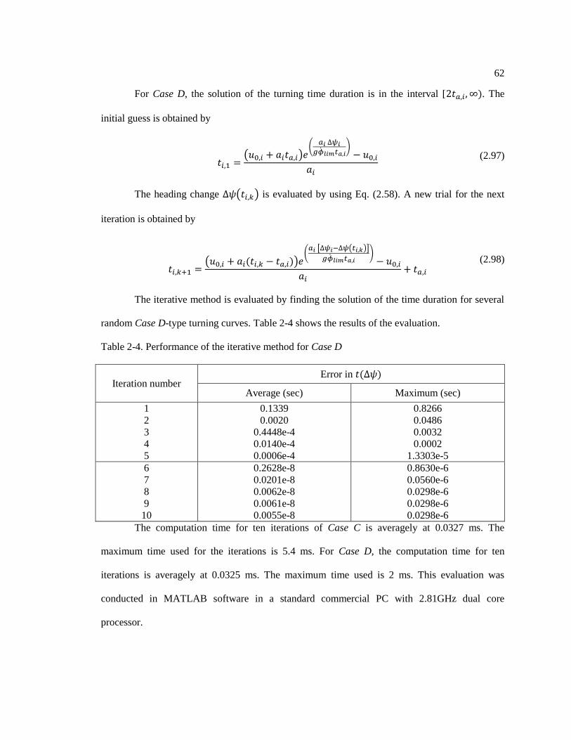
62
For Case D, the solution of the turning time duration is in the interval [ . The
initial guess is obtained by
( )
(
)
(2.97)
The heading change ( ) is evaluated by using Eq. (2.58). A new trial for the next
iteration is obtained by
( )
( [ ( )]
)
(2.98)
The iterative method is evaluated by finding the solution of the time duration for several
random Case D-type turning curves. Table 2-4 shows the results of the evaluation.
Table 2-4. Performance of the iterative method for Case D
Iteration number Error in
Average (sec) Maximum (sec)
1
2
3
4
5
0.1339
0.0020
0.4448e-4
0.0140e-4
0.0006e-4
0.8266
0.0486
0.0032
0.0002
1.3303e-5
6
7
8
9
10
0.2628e-8
0.0201e-8
0.0062e-8
0.0061e-8
0.0055e-8
0.8630e-6
0.0560e-6
0.0298e-6
0.0298e-6
0.0298e-6
The computation time for ten iterations of Case C is averagely at 0.0327 ms. The
maximum time used for the iterations is 5.4 ms. For Case D, the computation time for ten
iterations is averagely at 0.0325 ms. The maximum time used is 2 ms. This evaluation was
conducted in MATLAB software in a standard commercial PC with 2.81GHz dual core
processor.

63
2.4.2.6 Sorting Method
The three-point pattern (or bracketing the minimum) is a method to specify an interval in
the input domain in which a local minimum is located. The pattern is formed by three inputs and
three corresponding cost values where the intermediate input has the lowest cost value ( <
< and ( ) ( ) < ). This pattern implies that a local minimum lies
within the interval [ ]. Figure 2-18 illustrates the three-point pattern.
Figure 2-18. Three-point pattern and local minimum.
2.4.2.7 Stopping Criteria
Three stopping criteria are set for the planar path algorithm. The iterative algorithm will
stop if one of the three criteria is satisfied. The three criteria are (1) a planar path solution is found
( < ); (2) a solution that gives a minimum deviation at the destination is found by the
Golden Section method | | < ; and (3) the maximum number of iterations has been
reached. The maximum iteration number is used to limit the time spent computing the horizontal
path for each set of independent variables.
𝑡 𝑡 𝑡
𝐶 𝑡
𝐶 𝑡
𝐶 𝑡
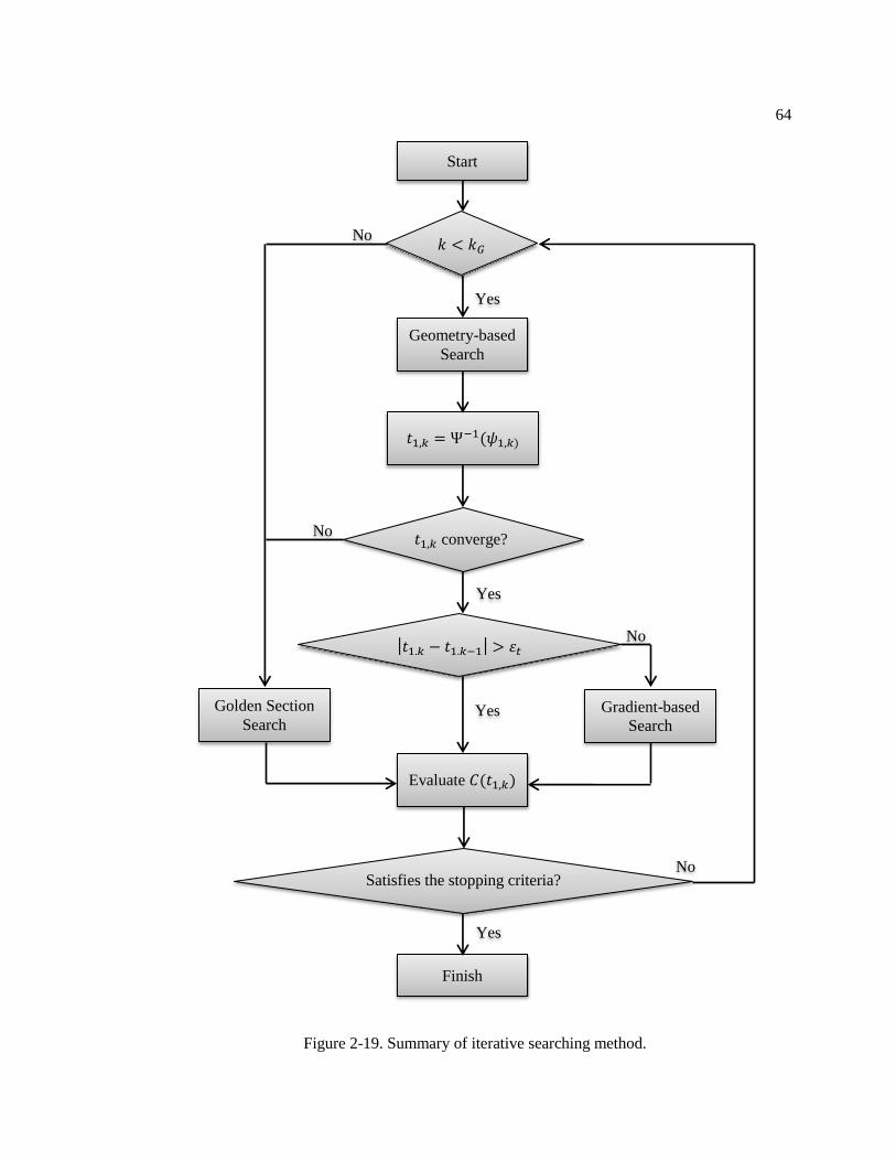
64
Figure 2-19. Summary of iterative searching method.
𝑘 < 𝑘𝐺
Start
Geometry-based
Search
Golden Section
Search Gradient-based
Search
𝑡 𝑘 converge?
|𝑡 𝑘 𝑡 𝑘 | 휀𝑡
𝑡 𝑘 Ψ 𝜓 𝑘
Evaluate 𝐶 𝑡 𝑘
Finish
Satisfies the stopping criteria?
Yes
Yes
Yes
Yes
No
No
No
No

65
Figure 2-20 shows samples of the planar paths computed for a set of path-defining
variables, [ ]. In this example, the aircraft
is initially at origin [0, 0], has an initial speed of 170 feet per second and is heading North. The
destination is 3,000 feet behind the aircraft and has a final speed of 80 feet per second and a final
heading to the north.
Figure 2-20. Horizontal path in no-wind condition for
Figure 2-21 shows samples of the planar paths, in the presence of wind from the west.
The path-defining parameters, and the initial and final conditions in this example are the same as
those in the previous example (Figure 2-20). In Figure 2-21, the wind with a magnitude of 10 feet
per second from the west is accounted for in the planar path computation.
-3000 -2000 -1000 0 1000 2000 3000-4000
-3000
-2000
-1000
0
1000
2000
East Position (ft)
Nort
h P
ositio
n (
ft)
Segment 1
Segment 2
Segment 3
Transition

66
Figure 2-21. Horizontal path in the presence of 10-feet-per-second wind from the west for
.
2.4.3 Quasi-steady State Autorotation
Along each segment of the autorotation descent path, the aircraft is assumed to be in
quasi-steady power-off autorotation. In order to find the vertical trajectory, the descent rate in this
condition at every point along the path must be known. For computational efficiency, a complete
mapping of all feasible operating points in quasi-steady autorotation is computed off-line and
modeled using an approximation function.
-3000 -2000 -1000 0 1000 2000 3000-4000
-3000
-2000
-1000
0
1000
2000
East Position (ft)
Nort
h P
ositio
n (
ft)
Segment 1
Segment 2
Segment 3
Transition

67
A quasi-steady autorotation is defined as a state with constant horizontal acceleration
( ), constant rotor speed ( ), constant bank angle, and zero net power required to drive
the rotor ( ). In addition, the states and controls must fall within the prescribed operating
limits of the aircraft (this includes limits on attitudes, airspeed, and rotor speed).
From the aircraft dynamics shown previously, the position vector of the aircraft has no
effect on the other aircraft states, and thus only three aircraft states (horizontal velocity, descent
rate, and rotor speed) are required in the power calculation to identify the autorotation flight.
When only these three states are taken into consideration, the rotorcraft dynamics become
[ ] [ ]
[ ] (2.99)
Applying the constraints of quasi-steady autorotation to Eq. (2.99), the states along each
flight segment are defined by the algebraic constraints
[
( )
] ([
] [
]) (2.100)
where is the segment number (the first turning segment, the straight segment, and the
second turning segment, respectively) and where are constants. Note that the
acceleration components, and , are in the same vehicle-carried coordinate system rotated
with the aircraft heading as the velocities, and .
In Eq. (2.100), the zero rate of change in the rotor speed, , implies that zero power
is required along each segment where rotor speed is prescribed by an algebraic constraint on the
required power, . Constant horizontal acceleration is used, so horizontal velocity changes
along the segment. In addition, the descent rate will vary over the segment in order to maintain
the quasi-steady autorotation condition. Unlike the horizontal acceleration, the rate of change of
the descent velocity, , will vary continuously over each segment. The instantaneous value of
descent acceleration, , can be computed using

68
⁄ (2.101)
where the derivative ⁄ is computed for all steady-state autorotation operating points. Note
that in low-speed autorotation, the required descent rate decreases when horizontal speed
increases ( ⁄ ). On the other hand, in a high-speed region, the required descent rate
increases when horizontal speed increases ( ⁄ < ).
Given values for the horizontal airspeed, acceleration, bank angle, and rotor speed,
[ ]
, Eq. (2.100) can be solved to find the corresponding descent rate, pitch attitude,
and thrust coefficient, { } , in the corresponding quasi-steady autorotation. In practical
autorotations, there are suggested constraints on the airspeed and rotor speed (e.g., the rotor speed
should be constrained to 90 to 105% of the rotor speed in normal flight conditions). Thus, a
mapping of the parameters, [ ]
, to the descent rate can be calculated numerically over
a well-defined range of values. In this work, the FSOLVE command in MATLAB is used for this
purpose. The resulting solutions were found to be a continuous hyperspace that defines a unique
mapping of [ ] to the input variables, [ ]
. The solutions are well-defined, but
computationally expensive to calculate. Figure 2-22 illustrates an example of quasi-steady
autorotation conditions.
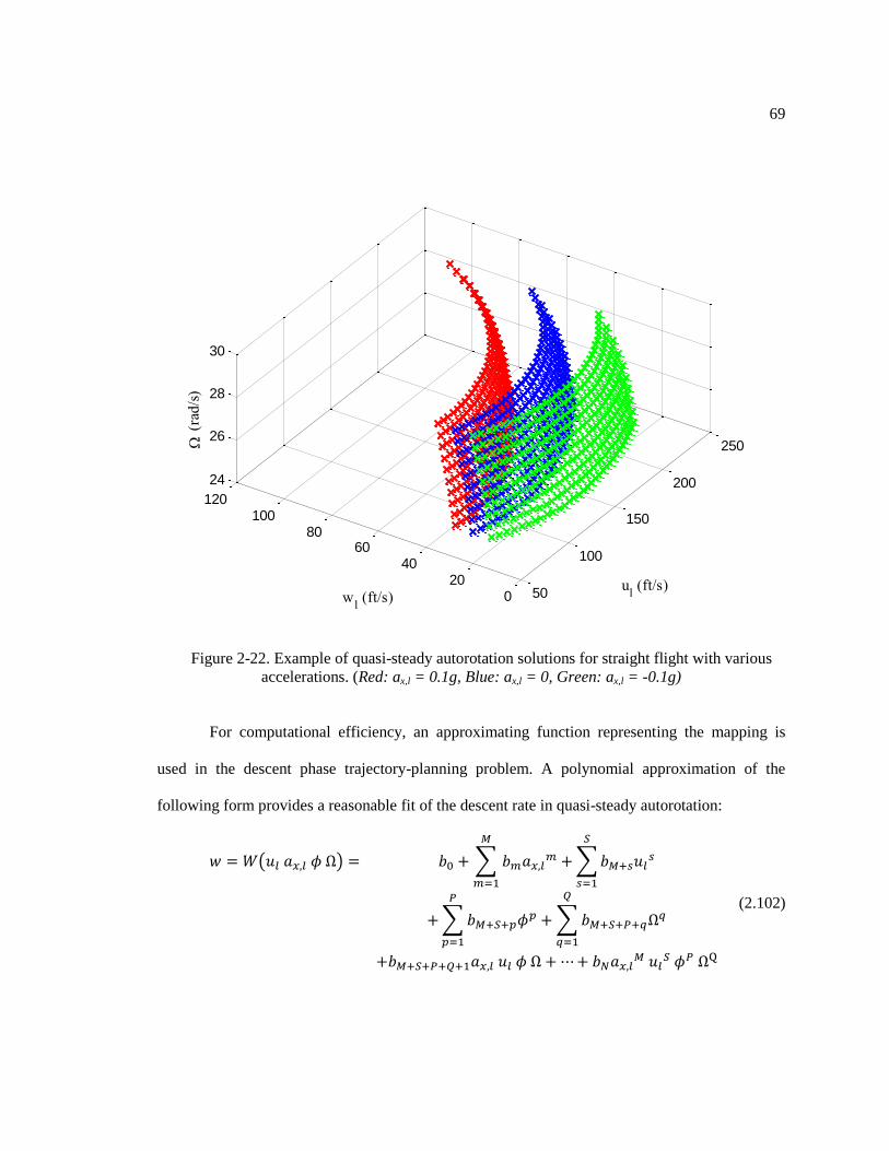
69
Figure 2-22. Example of quasi-steady autorotation solutions for straight flight with various
accelerations. (Red: ax,l = 0.1g, Blue: ax,l = 0, Green: ax,l = -0.1g)
For computational efficiency, an approximating function representing the mapping is
used in the descent phase trajectory-planning problem. A polynomial approximation of the
following form provides a reasonable fit of the descent rate in quasi-steady autorotation:
( ) ∑
∑
∑
∑
(2.102)
50
100
150
200
250
020
4060
80100
120
24
26
28
30
(
rad
/s)
wl (ft/s)
ul (ft/s)

70
The coefficients, , in Eq. (2.102) are calculated using a least-square estimation.
Approximating functions for the pitch angle and the thrust coefficient can also be obtained in a
similar way. These functions can be used to ensure that the thrust and pitch attitude for the quasi-
steady autorotation fall within practical constraints.
The descent height along each segment of the autorotation can be obtained by integrating
the descent rate approximating function:
∫ ∫ ( )
(2.103)
where .
2.4.4 Trajectory Planning Using Optimization
The autorotation trajectory-planning problem can be written as a parameter optimization
problem:
Minimize (2.104)
subject to
(2.105)
(2.106)
(2.107)
where
(2.108)
(2.109)
(2.110)
where is the initial altitude, is the desired altitude at the destination, is the nominal
rotor speed for the autorotation flight and the control parameter, , is defined by Eq. (2.47).

71
The nonlinear constraints, , are defined by the velocity at the end of the first turning
segment, the acceleration in the straight segment, and the velocity at the beginning of the second
turning segment:
[ ]
(2.111)
The primary objective in the cost function is to minimize the final altitude error at the
destination. The initial altitude, , the total altitude loss in each segment, and , and the
desired final altitude, , is used to formulated the cost due to final altitude error. The cost due
to deviation of rotor speed command from the nominal rotor speed for the autorotation flight, ,
is added in order to obtain an optimal trajectory solution in which the rotorcraft descents with the
rotor speed near the nominal rotor speed for the autorotation.
The nonlinear constraints are formulated by using the velocity at the end of the first
turning segment, the acceleration in the straight segment, and the velocity at the beginning of the
second turning segment. These parameters are obtained after the planar path solution is found for
the set of parametric control variables and the initial and terminal constraints. The parameters are
used to indicate the operating condition in the path solution. The nonlinear constraint function is
used to prevent any trajectory solution that requires the rotorcraft to operate outside the descent
phase operating boundary, e.g., the solution requires the acceleration in the straight segment
more/less than the limits.
In order to find an optimal solution in the Eq. (2.104), an optimizer must predict a set of
parametric control variables. The predicted parametric control variables are divided into two
group: (1) the independent variables of the planar path and (2) the vertical path variables. The
independent variables of the planar path are given to the iterative, searching algorithm in order to
find the planar path defining variables in Eq. (2.45) for the given set of independent variables and
the initial and terminal trajectory constraints. The obtained planar path defining variables and the
72
vertical path parametric control variables are applied to the approximation function of descent
velocity in order to find the altitude loss in each segment. The altitude loss in the trajectory and
the parameters indicating the operating condition are returned to the optimizer in which the cost
function and the nonlinear constraint function are evaluated and the next set of parametric control
variables is predicted. This iterative process must be repeated until an optimal solution is found.
Figure 2-23 to Figure 2-27 show examples of trajectory results from the descent phase
autorotation trajectory-planning algorithm. In Figure 2-23 and Figure 2-24, autorotation
trajectories that resulted from the algorithm are presented. These figures show four different
results for the following scenario: The demonstration aircraft is initially at 3,000 ft above the
target altitude and is heading north. The initial speed is 170 ft/s. The target destination is 3,000 ft
to the south from the initial position (that is, directly behind the aircraft). The target heading at
the destination is north. The scenario represents a case in which the aircraft turns completely
around, moves 3,000 ft behind its original location and then turns so that it heads north again.
There are many possible autorotation paths to the safe landing set. The algorithm finds an
available autorotation flight path in all types of paths. The resulting RSR, RSL, LSL, and LSR
paths are shown in Figure 2-23. This case also represents a scenario that should result in
symmetric solutions. The RSR and RSL paths are symmetric to the LSL and LSR paths,
respectively. The time histories for the paths in Figure 2-23 are shown in Figure 2-24. In Figure
2-24, the time histories for the LSL and LSR paths are the same as those for the RSR and RSL
path in most parameters with the exceptions of the bank angle and the heading, which differ
between the two figures only in regard to sign.

73
Figure 2-23. Example of a quasi-steady autorotation trajectory.
The vertical displacement error of each path-type solution is used to determine a safe
trajectory. In this scenario, the final altitude of the trajectory solution is within ±1 ft for all path
types. The RSL and LSR path types are considered too long. The helicopter must glide at a lower
rotor speed to reach the destination (Figure 2-24). However, the cost values also confirm the
effectiveness of the optimization algorithm in finding symmetric solutions for a symmetry
problem case.
-3000-2000
-10000
10002000
3000
-4000
-3000
-2000
-1000
0
1000
2000
0
500
1000
1500
2000
2500
3000
East Position (ft)
North Position (ft)
Alti
tude (
ft)
RSR
RSL
LSL
LSR

74
Figure 2-24. Time histories of the no-wind scenario.
The autorotation trajectories in the wind condition are shown in Figure 2-25. The time
histories of the trajectories in Figure 2-25 are shown in Figure 2-26 and Figure 2-27. In this
0 10 20 30 40 50 60 70 80 900
100
200V
eloci
ty (
ft/s
)
0 10 20 30 40 50 60 70 80 900
1000
2000
3000
Hei
ght (f
t)
0 10 20 30 40 50 60 70 80 901020304050
Des
cent ra
te (
ft/s
)
0 10 20 30 40 50 60 70 80 900
180
360
Hea
din
g (
deg
)
0 10 20 30 40 50 60 70 80 90-45
0
45
(d
eg)
0 10 20 30 40 50 60 70 80 90-4-2024
Acc
eler
atio
n (
ft/s
2)
0 10 20 30 40 50 60 70 80 9024
27
30
(
rad/s
)
time (s)
RSR
RSL

75
scenario, the final altitude of the trajectory solution is within ±1 ft for all types except the RSL
case. The effect of wind is advantageous for the LSR-type path, but disadvantageous for the RSL-
type path in this case.
Figure 2-25. Example of a quasi-steady autorotation trajectory in constant wind.
-3000
-2000
-1000
0
1000
2000
3000
-4000
-3000
-2000
-1000
0
1000
2000
0
1000
2000
3000
East Position (ft)North Position (ft)
Alti
tude (
ft)
RSR
RSL
LSL
LSR

76
Figure 2-26. Time histories of the constant wind scenario.
0 10 20 30 40 50 60 70 80 90 1000
100
200
Vel
oci
ty (
ft/s
)
0 10 20 30 40 50 60 70 80 90 1000
1000
2000
3000
Hei
ght (f
t)
0 10 20 30 40 50 60 70 80 90 1001020304050
Des
cent ra
te (
ft/s
)
0 10 20 30 40 50 60 70 80 90 1000
180
360
Hea
din
g (
deg
)
0 10 20 30 40 50 60 70 80 90 100-45
0
45
(d
eg)
0 10 20 30 40 50 60 70 80 90 100-4-2024
Acc
eler
atio
n (
ft/s
2)
0 10 20 30 40 50 60 70 80 90 10024
27
30
(
rad/s
)
time (s)
RSR
RSL

77
Figure 2-27. Time histories of the constant wind scenario. (Continued)
0 10 20 30 40 50 60 70 80 900
100
200
Vel
oci
ty (
ft/s
)
0 10 20 30 40 50 60 70 80 900
1000
2000
3000
Hei
ght (f
t)
0 10 20 30 40 50 60 70 80 901020304050
Des
cent ra
te (
ft/s
)
0 10 20 30 40 50 60 70 80 90-360
-180
0
Hea
din
g (
deg
)
0 10 20 30 40 50 60 70 80 90-45
0
45
(d
eg)
0 10 20 30 40 50 60 70 80 90-4-2024
Acc
eler
atio
n (
ft/s
2)
0 10 20 30 40 50 60 70 80 9024
27
30
(
rad/s
)
time (s)
LSL
LSR

78
2.4.5 Reachable Range Extension
The developed descent phase autorotation trajectory-planning algorithm considers the
initial height of the aircraft above the landing site as the available altitude and finds a turn-
straight-turn autorotation trajectory to fit that altitude. In this section, the case in which the
available altitude is not enough for the helicopter to perform the three-segment trajectory is
considered. This case represents a situation in autorotation flight where the initial aircraft altitude
is low and the desired landing site is far away.
To extend the reachable range, the constraint on the aircraft heading at the destination is
dropped. As the aircraft heading at touchdown is not restricted, the second turning segment,
which turns the aircraft to the desired heading, at the destination is not required. The descent
phase autorotation trajectory is reduced to a two-segment path, that is, a turn and a straight
segment. The parametric control variables of the descent phase trajectory are reduced to
{ }
(2.112)
The descent phase autorotation trajectory planning algorithm is modified such that it
drops sections involving the computation of the second turning segment. The straight segment,
which leads to the beginning of the second turn in the three-segment path is, instead, directed to
the destination. The geometry-based search in the planar path algorithm developed previously is
modified to find a heading change in the first turning segment, which minimizes the position error
between the end of the straight segment and the new destination ( ‖ ‖ ). Figure 2-28
shows the geometry-based search modified for the two-segment path. The new destination is
computed from the pre-calculated safe landing set for the target landing site and the heading in
the second segment:
(2.113)
(2.114)
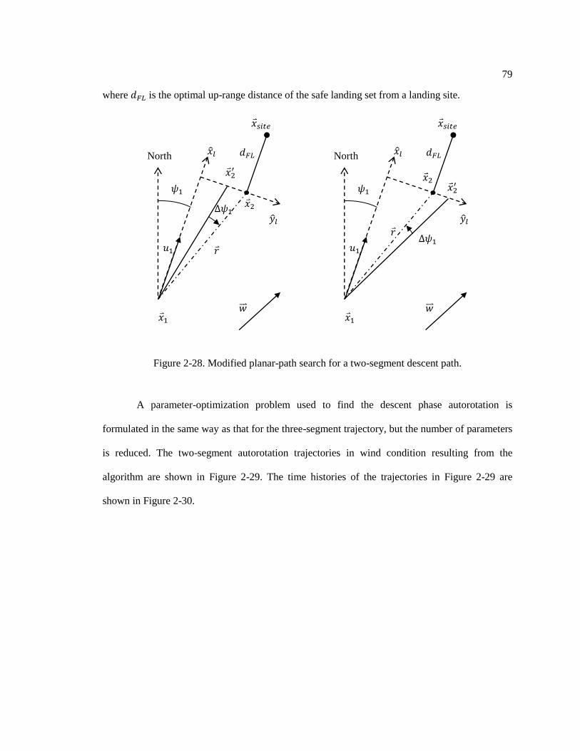
79
where is the optimal up-range distance of the safe landing set from a landing site.
Figure 2-28. Modified planar-path search for a two-segment descent path.
A parameter-optimization problem used to find the descent phase autorotation is
formulated in the same way as that for the three-segment trajectory, but the number of parameters
is reduced. The two-segment autorotation trajectories in wind condition resulting from the
algorithm are shown in Figure 2-29. The time histories of the trajectories in Figure 2-29 are
shown in Figure 2-30.
Δ𝜓 ��
𝜓
North 𝑥𝑙
��𝑙
��
��
��
𝑟 𝑢
𝑑𝐹𝐿
��𝑠𝑖𝑡𝑒
Δ𝜓
�� 𝜓
North 𝑥𝑙
��𝑙
��
��
��
𝑟
𝑢
𝑑𝐹𝐿
��𝑠𝑖𝑡𝑒

80
Figure 2-29. Example of a two-segment quasi-steady autorotation trajectory in constant wind.
-3000
-2000
-1000
0
1000
2000
3000
-4000
-3000
-2000
-1000
0
1000
2000
0
500
1000
1500
2000
2500
3000
East Position (ft)North Position (ft)
Alti
tude (
ft)
RS
LS
Initial Point
Destination
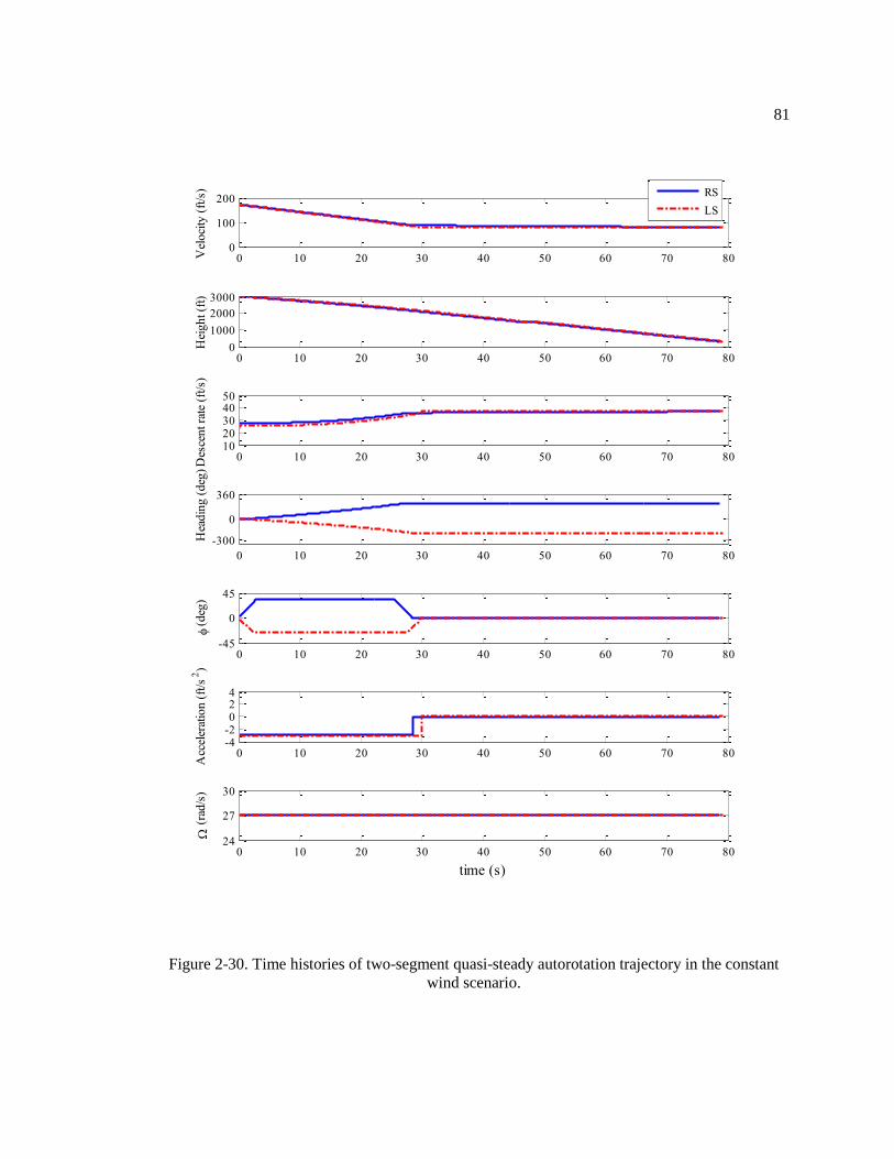
81
Figure 2-30. Time histories of two-segment quasi-steady autorotation trajectory in the constant
wind scenario.
0 10 20 30 40 50 60 70 800
100
200V
eloci
ty (
ft/s
)
0 10 20 30 40 50 60 70 800
1000
2000
3000
Hei
ght (f
t)
0 10 20 30 40 50 60 70 801020304050
Des
cent ra
te (
ft/s
)
0 10 20 30 40 50 60 70 80
-300
0
360
Hea
din
g (
deg
)
0 10 20 30 40 50 60 70 80-45
0
45
(d
eg)
0 10 20 30 40 50 60 70 80-4-2024
Acc
eler
atio
n (
ft/s
2)
0 10 20 30 40 50 60 70 8024
27
30
(
rad/s
)
time (s)
RS
LS

82
Figure 2-31. Example of reachable area for autorotation flight path.
Figure 2-31 show an example of the reachable area for an initial airspeed of 170 ft/s
regardless to the final heading. The rotorcraft initial position is indicated by a white mark. The
color contour illustrates an expansion of the reachable area as the initial altitude increases from
1,000 to 2,000 ft.
2.5 Flare Phase Path Generation
The objective of the flare phase path is to perform a safe autorotation landing. The flare
phase is designed to be a straight-in flight in which the rotorcraft holds constant heading while it
is slowing down the airspeed. In this section, two optimization methods are considered for the
computation the flare phase trajectories. The safe landing set method [11, 12] is adopted in the
first method, which discretizes the flare phase flight into small altitude intervals and aims to find
D
ista
nce
in f
orw
ard d
irec
tion (
ft)
Distance in lateral direction (ft)
-6000 -4000 -2000 0 2000 4000 6000
-2000
0
2000
4000
6000
8000
1000
1100
1200
1300
1400
1500
1600
1700
1800
1900
2000

83
the optimal control input over the entire flare trajectory. On the other hand, the second method
discretizes the flare flight into small time intervals and aims to find the optimal command inputs
for each time interval.
2.5.1 Safe Landing Set Method
The descent phase ends in the safe landing set, and a flare trajectory is followed for the
remainder of the flight. It is assumed that the flare trajectory begins from the trimmed
autorotation flight and that the heading is nearly constant (that is, there are no lateral deviations
from the path and it is a “straight in” approach). The safe landing set for the desired touchdown
point computed prior to the flights is the set of all the trimmed autorotation flight conditions and
flare initiation points that result in safe landing. This safe landing set is computed by finding the
optimal flare trajectory from a candidate flare initial condition to safe touchdown. If this optimal
trajectory exists then the candidate initial condition is a member of the safe landing set. Figure
2-32 shows the safe landing set of an example helicopter. The color contour indicates the number
of safe autorotation flights from the location. The blue color indicates unsafe region for flare
initiation. The red color indicates a region where safe autorotation flights are found for various
initial conditions. A detailed description and derivation of the safe landing set is given in [11, 12].
This derivation is briefly summarized here for completeness.

84
Figure 2-32. Example of a safe landing set. [11, 12]
A challenge in computing optimal flare trajectories is that the landing time is unknown.
However, the touchdown altitude is known, and the equations of motion are recast in terms of
altitude rather than in terms of time. Altitude is, thus, the independent variable for the purpose of
flare trajectory optimization, and touchdown time is computed as part of the process.
The desired touchdown condition for flare phase is
[
]
(2.115)
An optimal solution of the flare phase path is found by solving a trajectory-optimization
problem, which is cast as a nonlinear parameter-optimization problem by discretizing the vehicle
dynamics and finding control inputs that minimize a cost function.

85
The flare phase path is discretized into nodes by using the altitude. The vehicle states in
the next node are obtained by using a forward Euler integration of the vehicle states and control
inputs at the current node. The parameter optimization problem is
Minimize ({ }) (2.116)
subject to
(2.117)
(2.118)
( [ ]) (2.119)
(2.120)
[ ] [ ] [ ] (2.121)
where represents the pitch attitude response from the pitch command
( ) ( ) (2.122)
∑ (2.123)
Here, a barrier function is formed as
(2.124)
The computational tractability of the trajectory optimization is improved by
parameterizing inputs and using a cubic spline. The flare trajectory-optimization
problem is now a parameter-optimization problem. A trajectory following the controller
(discussed in the next chapter) follows the flare trajectory to touchdown. The dimension of the
parameter-optimization problem is reduced by decreasing the number of parameters, i.e.,
parameterized control inputs , representing the flare path. The control inputs at discretized
altitude nodes are generated by using a cubic spline fit:
{ } ({ }) (2.125)

86
where is a cubic spline fit function, N is the number of the smaller time step node, K is the
number of the bigger time step node, and .
In this study, the pitch attitude response from the pitch command is represented by the
following transfer function:
(2.126)
where is 2 rad/s and is 0.7
Figure 2-33 presents an example of the flare phase trajectory solution. In this figure, the
descent rate at touchdown is 7 feet per second. The final horizontal speed is 43 feet per second.
The displacement error at touchdown is 25 ft.

87
Figure 2-33. Example of a flare phase trajectory solution.
-20 0 200
50
100
150
200
250
300
Altitude (
ft)
(deg)
cmd
R
0 0.01 0.020
50
100
150
200
250
300
CT
20 25 300
50
100
150
200
250
300
(rad/s)
-600 -300 00
50
100
150
200
250
300
Altitude (
ft)
Distance (ft)
0 50 1000
50
100
150
200
250
300
Horizontal velocity (ft/s)
0 500
50
100
150
200
250
300
Vertical velocity (ft/s)

88
2.5.2 Backward Trajectory Generation Method for the Flare Phase Trajectory
The objective of this alternative flare trajectory generation method is to find the flare
trajectory that will land the rotorcraft at a specified condition. This method uses accepted
knowledge on the autorotation landing technique in order to compute a trajectory backwards from
touchdown to in-flight. Figure 2-34 illustrates the autorotation landing and path computation
process (numbers 1 to 4 indicate the main activities in the flare phase autorotation landing). The
flare landing starts from the steady state autorotation. The flare initiation is performed at a certain
altitude whereby the rotorcraft pitches up and starts to decelerate (number 4). The high pitch
deceleration continues until the rotorcraft reaches a certain altitude (number 3). Then, the
rotorcraft decreases its pitch attitude until level to the ground (number 2). Finally, the rotorcraft
prepares for the impact of touchdown and lands safely (number 1).
Figure 2-34. Flare autorotation landing technique and computation process of the flare trajectory.
Steady State
Autorotation High Pitch:
Decrease
Airspeed Leveling the pitch:
Prepare for
Touchdown
Pitching-up:
Flare Initiation
Touchdown
1
Minimize:
- Change in Velocities
- Rotor Speed Drop, Ω <
2
Specify:
- Pitch Attitude
Minimize:
- Rotor Speed Drop,
Ω <
3
Minimize:
- Rotor Speed Drop
- Change in Forward
Speed
4
Minimize the
Changes in
Airspeed and
Rotor Speed
Autorotation Activity
Path Computation Process
89
In order to generate the trajectory, the path is discretized in a backward-time way. The
touchdown condition, i.e., position, horizontal speed, descent velocity, and rotor speed, is
specified. The initial condition of the flare path is specified but is not considered as the path
constraint (i.e., there can be slight differences in the initial condition of the solution from the
specified condition). The specified initial condition is used to determine the time duration of the
flare path. The control inputs at each time node are the parameters in the optimization method
that are solved to satisfy the objectives of the main activities, as shown in Figure 2-34. The
computation starts from the touchdown condition and goes backward until a steady state flight
condition near the given initial condition is obtained. The path computation process starts by
finding the optimal control inputs for the specified touchdown condition at the final time node.
The control input solution and the rotorcraft condition at the current time node are used to
compute the vehicle condition at the previous time node (one time step in the past). This process
is repeated until the optimal control inputs for all the time nodes in the flare path have been
obtained. During this repeated process, the objective function used to determine the optimal
control inputs is selected according to the four tasks necessary for autorotation landing.
The computation process starts with the last action in the autorotation (number 1). The
objective of this task is to maintain the touchdown velocities and pitch attitude for the specified
time duration, , before the touchdown occurs. The control inputs are optimized to minimize
the change in airspeed regardless of the decrease in rotor speed.
When the computation reaches the specified time node, , the objective changes. The
second objective function (number 2) is used in the task that begins when the helicopter has a
high pitch-attitude flare and ends when the pitch attitude renders the rotorcraft level to the ground
(at seconds before the touchdown). The objective of this task is to decrease the horizontal
velocity from the initial condition to the touchdown condition. In this task, the rotorcraft is
designed to have the maximum allowed pitch attitude at the start and to decrease the pitch at the

90
maximum allowed pitch rate such that zero pitch is achieved at the end. The pitch attitude during
this task is specified in the path computation. The computation starts at the rotorcraft condition at
seconds and continues until a certain horizontal velocity near the desired initial condition is
reached.
When the path computation reaches the time node at which the specified velocity is
obtained, the objective changes to that specified at number 3. This task begins when the flare is
initiated and ends when the maximum pitch attitude is reached. The objective of this task is to
maintain horizontal speed and bring the rotorcraft from steady state autorotation to the condition
at the point connecting to the previous task. The objective function of this task is designed to
minimize the change in horizontal velocity and penalize solutions that increase rotor speed
deviation from the desire initial condition.
Finally, the fourth objective is used when the path computation reaches a steady
autorotation. This final objective is to maintain the steady state autorotation condition. In the
computation process, the fourth objective function is used to extend the flare path and ensure that
the flare path starts with a steady state autorotation.
The parameter-optimization problem for each time node can be written as
Minimize (2.127)
subject to
[
] (2.128)
(2.129)
(2.130)
(2.131)

91
where represents the helicopter dynamics, [ ], is the maximum
allowed change of the control inputs, is the cost function specified differently for each main
activity objective, i indicates the main activity number, , and k is the current iteration
number.
It was found that the main activity objective functions in the following form yield
reasonable results:
(2.132)
(2.133)
(2.134)
(2.135)
where
(2.136)
(2.137)
(2.138)
where is the current rotor speed in rad/s and is the desired initial rotor speed of the flare
path in rad/s.
Figure 2-35 shows the solution of the flare phase trajectory for the touchdown condition
of 40 ft/s horizontal speed, 5 ft/s descent rate, and 70% RPM. In the result, the path is specified in
order to keep the touchdown velocity for 0.5 seconds before touchdown ( ) and has an
overall time of 9 seconds ( ).

92
Figure 2-35. Example of a flare phase trajectory solution from the backward trajectory generation
algorithm.
0 1 2 3 4 5 6 7 8 9-10
0102030
R (
deg)
0 1 2 3 4 5 6 7 8 90
0.005
0.01
CT
0 1 2 3 4 5 6 7 8 90
50
100
ul (
ft/s
)
0 1 2 3 4 5 6 7 8 90
50
wl (
ft/s
)
0 1 2 3 4 5 6 7 8 9
20
25
30
(
rad/s
)
Time (s)

Chapter 3
Autonomous Control
This chapter presents the development of the control law to command the autonomous
autorotation landing maneuver for a helicopter. The control architecture consists of an inner loop,
the primary flight control system that tracks aircraft attitude commands, and an outer loop, which
follows trajectory commands (as shown in Figure 3-1). Both the inner loop and the outer loop
flight control laws are model following schemes with dynamic inversion.
Figure 3-1. Schematic of an autonomous control and path-planning system.
3.1 Inner-loop Linear Dynamic Inversion Control
The linear dynamic inversion design scheme is selected to provide stability to the
rotorcraft. The inner-loop control law follows attitude commands in the roll and pitch axes, and
the yaw rate commands the yaw axis. The collective input comes from the outer-loop control law
and simply passes through the inner loop so that the inner-loop inverse model can account for the
Linear
Dynamic
Inversion
Rotorcraft
Dynamics
Autorotation
Trajectory
Generation
Nonlinear
Position
Dynamic
Inversion
Aircraft
Attitude
Command
Inner Loop
Outer Loop
Trajectory
Command
Current
Aircraft
Condition

94
collective coupling effects. Figure 3-2 shows a schematic of the linear dynamic inversion control
scheme for the rotorcraft primary flight control.
Figure 3-2. Schematic of the linear dynamic inversion control system for primary flight control.
3.1.1 Desired Response
The rotorcraft inner loop response characteristics were chosen to be an Attitude
Command/Attitude Hold (ACAH) type for the roll and pitch axes and a Rate Command/Attitude
Hold (RCAH) type for the yaw axis. For the roll and pitch axes, the bank angle and the pitch
attitude were specified as command inputs, respectively. A second-order command filter was
used to compute the desired response for the attitude control.
The desired response in the roll and pitch axes is described by
(3.1)
(3.2)
For the yaw axis, the yaw rate was set as the command input. The yaw axis used a first-
order command filter:
(3.3)
[ 𝛿𝑙𝑎𝑡𝛿𝑙𝑜𝑛𝛿𝑐𝑜𝑙𝛿𝑝𝑒𝑑]
Inversion
Model
Rotorcraft
Dynamics Euler Angle
Conversion
Error
Dynamics
PID: ACAH
PI: RCHH
Command
Filters
[𝜙 𝜃 𝑝 𝑞 𝑟 𝑉]𝑇
[
��𝐷��𝐷��𝐷
] [��
��𝑟
]
[��𝑐 ��𝑐 ��𝑐]𝑇
[𝜙𝑐𝑚𝑑
𝜃𝑐𝑚𝑑
𝑟𝑐𝑚𝑑
]
𝛿𝑐𝑜𝑙 𝑐𝑚𝑑

95
In the present study, a natural frequency of 2 rad/s and a damping ratio of 0.7 were
selected for the roll and pitch command filters. The maximum roll and pitch attitude changes
were set at 45º (0.7854 rad) and 30º (0.5236 rad), respectively. For the yaw axis, a time constant
of 0.4 seconds was chosen. The maximum yaw rate of 60 deg/s (1.0472 rad/s) was selected.
3.1.2 Inversion Model
A simple third-order model of angular rate dynamics was used as the reference model for
the rotorcraft dynamics. This simple model was linearized from the high-fidelity nonlinear
FLIGHTLAB rotorcraft simulation model:
[
] [ ] [ ] [ ]
[ ]
(3.4)
As the collective command comes from the outer-loop controller, the reference can be
written as
[
] [ ] [ ] [ ] [
] [ ] (3.5)
For the desired angular accelerations, the corresponding control inputs can be obtained by
using the model-inversion technique. The inversion model is
[
] [ ] ([
] [ ] [ ] [ ] ) (3.6)
The inversion model is scheduled with airspeed to account for changes in the rotorcraft
dynamics due to changes in airspeed. The scheduling airspeeds include normal operating
conditions from hover to a forward flight speed of 160 knots, at the sea-level standard.
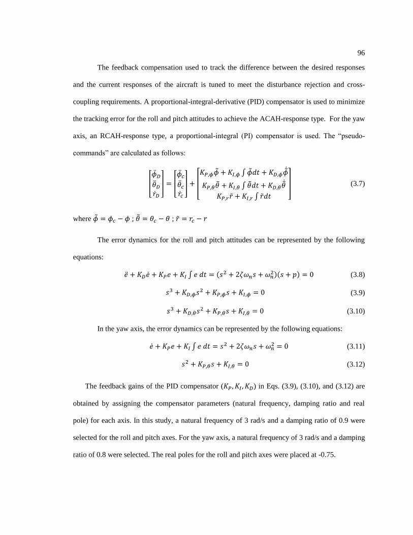
96
The feedback compensation used to track the difference between the desired responses
and the current responses of the aircraft is tuned to meet the disturbance rejection and cross-
coupling requirements. A proportional-integral-derivative (PID) compensator is used to minimize
the tracking error for the roll and pitch attitudes to achieve the ACAH-response type. For the yaw
axis, an RCAH-response type, a proportional-integral (PI) compensator is used. The “pseudo-
commands” are calculated as follows:
[
] [
] [
∫
∫
∫
] (3.7)
where ; ;
The error dynamics for the roll and pitch attitudes can be represented by the following
equations:
∫ (3.8)
(3.9)
(3.10)
In the yaw axis, the error dynamics can be represented by the following equations:
∫ (3.11)
(3.12)
The feedback gains of the PID compensator ( ) in Eqs. (3.9), (3.10), and (3.12) are
obtained by assigning the compensator parameters (natural frequency, damping ratio and real
pole) for each axis. In this study, a natural frequency of 3 rad/s and a damping ratio of 0.9 were
selected for the roll and pitch axes. For the yaw axis, a natural frequency of 3 rad/s and a damping
ratio of 0.8 were selected. The real poles for the roll and pitch axes were placed at -0.75.
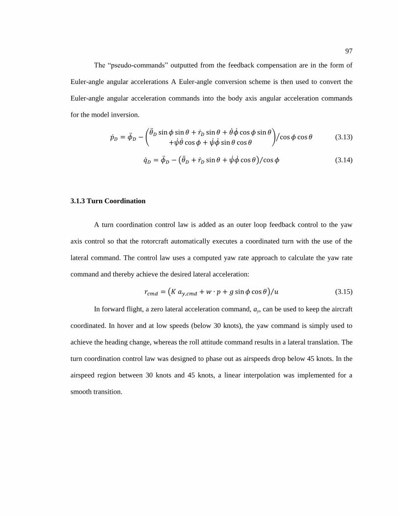
97
The “pseudo-commands” outputted from the feedback compensation are in the form of
Euler-angle angular accelerations A Euler-angle conversion scheme is then used to convert the
Euler-angle angular acceleration commands into the body axis angular acceleration commands
for the model inversion.
(
) ⁄ (3.13)
( ) ⁄ (3.14)
3.1.3 Turn Coordination
A turn coordination control law is added as an outer loop feedback control to the yaw
axis control so that the rotorcraft automatically executes a coordinated turn with the use of the
lateral command. The control law uses a computed yaw rate approach to calculate the yaw rate
command and thereby achieve the desired lateral acceleration:
( ) ⁄ (3.15)
In forward flight, a zero lateral acceleration command, ay, can be used to keep the aircraft
coordinated. In hover and at low speeds (below 30 knots), the yaw command is simply used to
achieve the heading change, whereas the roll attitude command results in a lateral translation. The
turn coordination control law was designed to phase out as airspeeds drop below 45 knots. In the
airspeed region between 30 knots and 45 knots, a linear interpolation was implemented for a
smooth transition.
98
3.2 Outer-loop Nonlinear Inversion Control
The outer-loop path following the control law is designed to calculate the inner-loop
commands in order to maneuver the aircraft along the desired path. Decoupled control laws are
used for the longitudinal, lateral, and vertical axes. The acceleration components in the local
frame are used to generate the pitch angle, the bank angle, and the collective commands,
respectively. A PID compensator is added to minimize the tracking path error in each axis. Figure
3-3 illustrates the outer-loop control diagram.

Figure 3-3. Autonomous autorotation control diagram.
Inner-loop
Inversion
Model
[ 𝛿𝑙𝑎𝑡𝛿𝑙𝑜𝑛𝛿𝑐𝑜𝑙𝛿𝑝𝑒𝑑]
Rotorcraft
Dynamics 𝐿 PID
Compensator
Command
Filters
[𝑥 𝑦 𝑧 𝜃 𝜙 𝜓 𝛽]𝑇
𝜙𝑐𝑚𝑑
𝜃𝑐𝑚𝑑
[
𝑒𝑥𝑒𝑦𝑒𝑧] [
𝑥𝑐𝑚𝑑
𝑦𝑐𝑚𝑑
𝑧𝑐𝑚𝑑
]
𝛿𝑐𝑜𝑙 𝑐𝑚𝑑
[
𝑎𝑥 𝑙 𝑐𝑚𝑑
𝑎𝑦 𝑙 𝑐𝑚𝑑
𝑎𝑧 𝑙 𝑐𝑚𝑑
]
𝐾𝛽
𝑎𝑦 𝑐𝑚𝑑
Turn
Coordination
[𝜙𝑐𝑚𝑑
𝜃𝑐𝑚𝑑
𝑟𝑐𝑚𝑑
]
𝛽
𝜙𝑡𝑟𝑖𝑚
𝜃𝑡𝑟𝑖𝑚
𝛿𝑐𝑜𝑙 𝑡𝑟𝑖𝑚

The following simplified equations of helicopter motion (expressed in its local coordinate
frame) are used to formulate the control law:
(3.16)
(3.17)
(3.18)
where
[
] [
] (3.19)
Linearizing Eqs (3.16)–(3.18) gives
(3.20)
(3.21)
(3.22)
For the steady-state flight condition ( ),
(3.23)
(3.24)
(3.25)
Eqs. (3.20)-(3.22) become
(3.26)
(3.27)
(3.28)
Assuming that,
(3.29)

101
(3.30)
where is the control derivative modeling vertical acceleration response to the collective
command.
A linear reference model is obtained
[
] [ ] [
] (3.31)
where
[
]
(3.32)
The inversion model, which computes the required pitch angle, the bank angle, and the
collective command from the desired translational acceleration can be obtained:
[
] [ ] [
] (3.33)
where
[
]
(3.34)
For simplification, the coupling terms are not included:
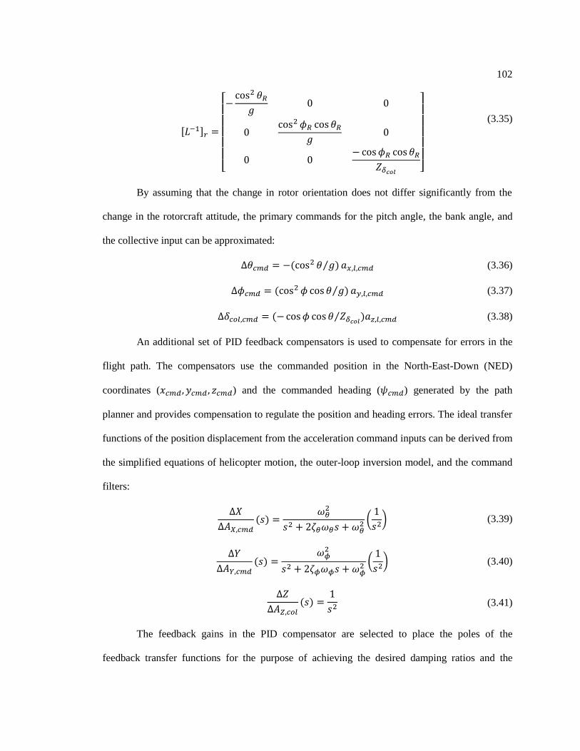
102
[ ]
[
]
(3.35)
By assuming that the change in rotor orientation does not differ significantly from the
change in the rotorcraft attitude, the primary commands for the pitch angle, the bank angle, and
the collective input can be approximated:
⁄ (3.36)
⁄ (3.37)
⁄ (3.38)
An additional set of PID feedback compensators is used to compensate for errors in the
flight path. The compensators use the commanded position in the North-East-Down (NED)
coordinates ( ) and the commanded heading ( ) generated by the path
planner and provides compensation to regulate the position and heading errors. The ideal transfer
functions of the position displacement from the acceleration command inputs can be derived from
the simplified equations of helicopter motion, the outer-loop inversion model, and the command
filters:
(
) (3.39)
(
) (3.40)
(3.41)
The feedback gains in the PID compensator are selected to place the poles of the
feedback transfer functions for the purpose of achieving the desired damping ratios and the

103
natural frequencies of the displacement error feedback system on each axis. The path-following
control laws combine the primary command and error compensating command to generate
command inputs for the inner-loop control system (Figure 3-1):
( ∫ ) (3.42)
( ∫ ) (3.43)
( ∫ ) (3.44)
where is a constant bank angle command that the path planner assigns for a coordinated
flight in the turning segments of the autorotation trajectory.
The error terms, , are components of the position error vector in the local
coordinate frame as calculated by
{
} [
]
(3.45)
The derivative, , is obtained from the linearization of the rotorcraft model and was
found to vary moderately with airspeed. However, it was found that a constant value gave
reasonable controller performance. The poles of the feedback transfer functions for the
longitudinal and lateral axes are placed at , and
by the selection of the feedback gains ( ). For the vertical
axis, the poles of the feedback transfer functions are placed at and by
the selection of the feedback gains ( ).
The yaw control receives no path-following command from the outer-loop controller. In
the power-off autorotation flight, it is assumed that the rotorcraft is in a zero sideslip coordinated
flight, in which the heading is always aligned with the flight path. Therefore, the yaw command is

104
simply used to reject disturbance in the lateral axis. The pedal command of the inner-loop control
system is used to minimize the vehicle’s sideslip angle:
(3.46)

Chapter 4
Implementation and Real-Time Simulation Results
This chapter describes the implementation of the autonomous autorotation system for use
in real-time high fidelity full-dynamics helicopter simulation flights at a flight simulation facility
at the Penn State Vertical Lift Research Center of Excellence (VLRCOE). Details regarding the
implementation of the trajectory-planning algorithms, the inner-loop flight control, and the path-
following control law in the simulator are described. Problems related to real-time operation and
software communication are also discussed. Finally, results from the real-time simulation are
presented.
4.1 Flight Simulation Description
The flight simulation facility at the Penn State Vertical Lift Research Center of
Excellence (VLRCOE) is a PC-based and re-configurable type simulator (i.e., the facility can be
used for different aircraft models). The rotorcraft dynamics are represented using the
FLIGHTLAB software. The simulation process is presented in Figure 4-1. The control loading
system tracks displacement in the cockpit inputs. The cab interface receives and passes the
commands (displacements) to FLIGHTLAB. The rotorcraft dynamics output from FLIGHTLAB
is sent to the image processing unit where the corresponding pilot view is generated based on the
rotorcraft attitude and position relative to the terrain map.

106
Figure 4-1. Simulation process diagram.
FLIGHTLAB is an aircraft modeling and analysis tool developed by Advanced
Rotorcraft Technology (ART). The software allows the user to produce rotorcraft models
interactively, to test and evaluate models, and to perform real-time simulations of models. The
software provides a graphical user interface (GUI) that allows users to easily create, evaluate, and
simulate rotorcraft models. The environment setting (wind condition) can be changed using the
GUI.
FLIGHTLAB software provides Control System Graphical Editor (CSGE) in which a
flight control system can be built and integrated with the rotorcraft dynamic model. A power-off
condition is simulated by disconnecting the engine system from the rotor system during flight. A
switch to disengage the engine during simulated flights was implemented through CSGE.
FLIGHTLAB also provides HELIFLIGHT which is the software in which rotorcraft
models created from FLIGHTLAB can be selected for real-time simulation. The HELIFLIGHT

107
program not only operates the aircraft model but manages the data transfer to the image
generation unit as well. The non-linear FLIGHTLAB simulation model of a generic utility
helicopter is used to evaluate the trajectory-generating algorithm in this software.
The Cab Interface works as a connection to pass external commands from the control
loading system to FLIGHTLAB. Commands are handled in the simulation loop by using a
Fortran program. Data transfer between the Cab Interface and FLIGHTLAB is managed by
software provided by FLIGHTLAB. The rate of the simulation loop (command update rate) is
adjustable and is generally specified at 20Hz.
4.2 Implementation for Real-time Simulated Flights
In order to have the autonomous autorotation system to run in real-time simulation, two
other computing units were required. One of the units was responsible for commanding the
rotorcraft in real-time; another was responsible for the other required computation (i.e. the path
generation). A standard commercial PC with a 2.81GHz dual core processor and Windows XP
Professional 2002 operating system was used in this task. The computer was connected to the
simulation process such that a network communication was established between the Cab Interface
computer and the PC. The communication was facilitated through a UDP network connection. On
the PC side, two MATLAB process sessions were operated simultaneously to compute the real-
time helicopter commands and to simultaneously generate the autorotation trajectory solution.
The data transfer between these two MATLAB sessions was achieved using shared memory.
Figure 4-2 shows how the many aspects of the autonomous autorotation system were connected.

108
Figure 4-2. Network communication between the autonomous system and the flight
simulator.
The system involving algorithms and control laws presented in Chapters 2 and 3 was
divided into four parts: the flight control system, the flight director, the path planner, and the
trajectory database. The flight control system was designed to provide stability in both the normal
condition and the autorotation condition. The control law was implemented in FLIGHTLAB
software using CSGE. The flight director used the outer-loop control law to provide control
commands continuously throughout the autorotation flight, and the path planner used the
autorotation trajectory algorithm to generate trajectory solutions. Both of these were
implemented in MATLAB software.
MATLAB2:
Path Planner
Cab
Interface
(Linux)
FLIGHTLAB
(Inner loop
Controller)
MATLAB1:
Flight
Director
(Outer-loop
Control Law)
Entry Phase
Database
UDP
Connection
Shared
Memory
AUTONOMOUS
AUTOROTATION SYSTEM
(PC: Windows XP)
Flare Phase
Database
UDP
Connection
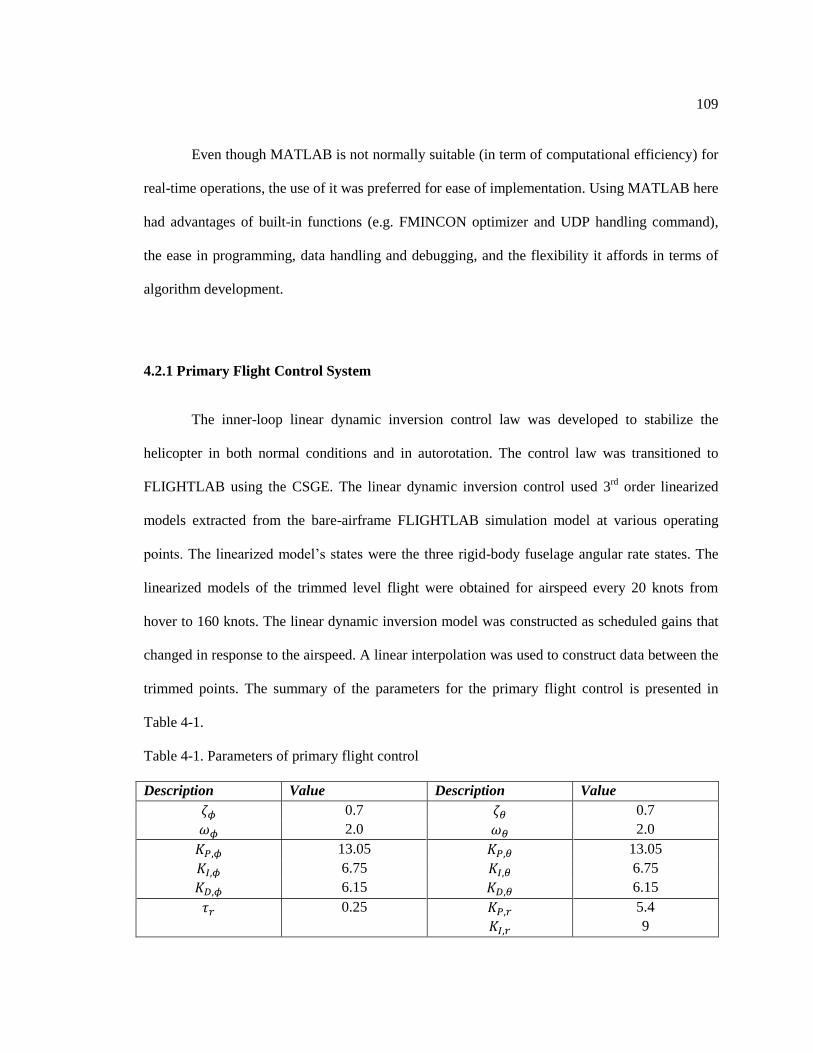
109
Even though MATLAB is not normally suitable (in term of computational efficiency) for
real-time operations, the use of it was preferred for ease of implementation. Using MATLAB here
had advantages of built-in functions (e.g. FMINCON optimizer and UDP handling command),
the ease in programming, data handling and debugging, and the flexibility it affords in terms of
algorithm development.
4.2.1 Primary Flight Control System
The inner-loop linear dynamic inversion control law was developed to stabilize the
helicopter in both normal conditions and in autorotation. The control law was transitioned to
FLIGHTLAB using the CSGE. The linear dynamic inversion control used 3rd
order linearized
models extracted from the bare-airframe FLIGHTLAB simulation model at various operating
points. The linearized model’s states were the three rigid-body fuselage angular rate states. The
linearized models of the trimmed level flight were obtained for airspeed every 20 knots from
hover to 160 knots. The linear dynamic inversion model was constructed as scheduled gains that
changed in response to the airspeed. A linear interpolation was used to construct data between the
trimmed points. The summary of the parameters for the primary flight control is presented in
Table 4-1.
Table 4-1. Parameters of primary flight control
Description Value Description Value
0.7 0.7
2.0 2.0
13.05 13.05
6.75 6.75
6.15 6.15
0.25 5.4
9
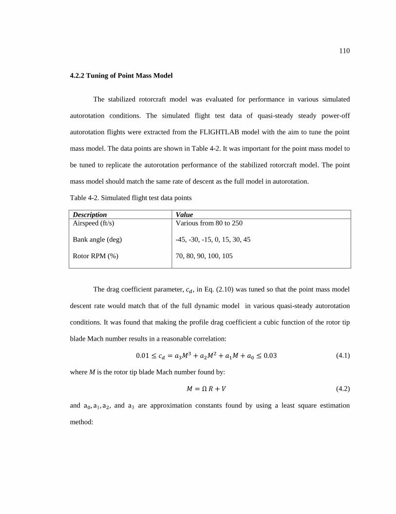
110
4.2.2 Tuning of Point Mass Model
The stabilized rotorcraft model was evaluated for performance in various simulated
autorotation conditions. The simulated flight test data of quasi-steady steady power-off
autorotation flights were extracted from the FLIGHTLAB model with the aim to tune the point
mass model. The data points are shown in Table 4-2. It was important for the point mass model to
be tuned to replicate the autorotation performance of the stabilized rotorcraft model. The point
mass model should match the same rate of descent as the full model in autorotation.
Table 4-2. Simulated flight test data points
Description Value
Airspeed (ft/s)
Various from 80 to 250
Bank angle (deg)
-45, -30, -15, 0, 15, 30, 45
Rotor RPM (%)
70, 80, 90, 100, 105
The drag coefficient parameter, , in Eq. (2.10) was tuned so that the point mass model
descent rate would match that of the full dynamic model in various quasi-steady autorotation
conditions. It was found that making the profile drag coefficient a cubic function of the rotor tip
blade Mach number results in a reasonable correlation:
(4.1)
where M is the rotor tip blade Mach number found by:
(4.2)
and 1 and are approximation constants found by using a least square estimation
method:

111
[
]
[
]
[
] (4.3)
[
] [ ] [ ] [ ] [
] (4.4)
where K is the number of flight test data points.
Figure 4-3 shows the correlation between the descent rate of the FLIGHTLAB model and
that of the tuned point mass model at various autorotation operating conditions. Data points in the
figure correspond to autorotation operating conditions at airspeeds between 40 and 250 ft/s,
accelerations between -3 and 1 ft/s2, rotor speeds between 24 and 29 rad/s and bank angles of 0,
15, and 30 deg.
Figure 4-3. Correlations between the point mass model and the FLIGHTLAB model.
10 20 30 40 5010
20
30
40
50
Po
int m
ass
mo
del
des
cen
t ra
te (
ft/s
)
FLIGHTLAB model descent rate (ft/s)

112
From the simulated autorotation flight test, it was found that autorotation flights with a 45
º bank angle required much higher sink rates than the rest of data points. Therefore, a maximum
bank angle of 30º was specified for the autorotation trajectory generation.
4.2.3 Trajectory Generation Overview
The tuned point mass model was used in the three autorotation path algorithms. Recall
that there are two entry phase trajectory generating algorithms and two methods of flare phase
trajectory-generating algorithms presented in Chapter 2. For the entry phase, the second entry
phase trajectory-generating algorithm was used to find the entry phase trajectory solutions for the
demonstration helicopter. This method was selected because the high level of consistency of the
solutions it generates enables path solutions to be approximated by using a linear interpolation of
the boundary solutions.
For the flare phase, the backward trajectory-generating method was used since a better
touchdown condition was found. The touchdown limitations for the generic utility helicopter
were designated as those of a UH-60 helicopter. The limitations of the UH-60 helicopter’s
landing gear comprised the following: (1) a maximum touchdown sink rate of 9 ft/s on level
terrain for a helicopter with a gross weight of up to 16,825 lbs., and (2) a maximum ground speed
of 60 knots on level terrain [88]. The flare phase trajectory solution was generated for the
touchdown sink rate of 5 ft/s and ground speed of 23.7 knots (40 ft/s). The starting condition of
the flare trajectory solution for the demonstration helicopter was obtained at a 707 ft uprange and
262 ft above the target landing site and used to specify the target point for the descent phase
trajectory.

113
As it was possible for the end of the descent phase trajectory to be at the different altitude
from the specified target, an update to the flare-phase trajectory was required. In the present
work, the descent-phase trajectory was considered unsuccessful if the altitude difference between
the end of the descent trajectory solution and the target altitude for the flare initiation was larger
than 20 ft. Alternative flare-phase trajectories were created for the same initial horizontal airspeed
at different altitudes. A linear interpolation of the boundary alternative solutions was used to
update the flare trajectory according to the altitude at the end of the descent-phase trajectory in
real time.
4.2.4 Pre-flight Computation
The entry and flare phase algorithms were developed in MATLAB. The tuned point mass
model was implemented for the evaluation of the cost functions. The MATLAB FMINCON
function was used as an optimizer to solve the entry phase and flare phase parameter optimization
problems. The entry phase solutions were obtained for airspeed at every 10 ft/s from hover to 250
ft/s. Solutions to the entry phase path were stored in the database for the flight director. For the
flare phase, the algorithm was used to find the main solution for the specified touchdown
condition and for alternative solutions for altitudes between 242 and 282 ft above the landing site.
The flare phase solutions were stored in the path planner.
For the descent phase algorithms, the tuned point mass model was used to create quasi-
steady autorotation data points in the operating boundary of the descent phase trajectory. The
MATLAB FSOLVE function was used to find the trimmed flight conditions in the point mass
model. The descent rate approximation function in Eq.(2.102) was obtained from these data

114
points via a least square method. Table 4-3 shows details pertaining to the generated data points
and the designated descent phase operating conditions.
Table 4-3. Quasi-steady autorotation data points generated for the approximation function
Description Generated data point Descent phase operation
Horizontal airspeed (ft/s)
Every 5 from 80 to 250 Between 50 and 240
Horizontal acceleration (ft/s2)
Every 0.8 from -4 to 4
Within ±3.217
Rotor RPM (rad/s)
Bank angle (deg)
Every 0.5 from 24 to 29
Every 5 from 0 to 30
Between 24.3 and 28.4
0 for straight segment
5–30 for turning segment
In order to ensure the feasibility of the quasi-steady autorotation path, the approximation
function was adjusted to cover all the under-estimated points. The approximated descent rate
would always be higher than the required descent rate. This higher approximated descent rate in
the path would result in a higher-than-required operating rotor speed, which would decrease the
gliding distance in the path. However, the higher approximated descent rate could guarantee that
the path wouldn’t result in a maneuver at a rotor speed below the lower limit. The 5º lower limit
on the bank angle for the turning segments was used to prevent large radius turns, which tend to
cause numerical problems in the optimization solution. This limit forces the optimizer to give
RSR, RSL, LSL, and LSR path type solutions.
4.2.5 Path Planner (In-flight Operation)
The path planner computed the descent trajectory in the real-time simulation. Developed
in MATLAB, this program was designed to await commands from the flight director, and to
compute and return the trajectory solution. The data transfer with the flight director was achieved

115
using shared memory established by the MATLAB MEMMAPFILE function. The descent phase
algorithm described in Chapter 2 was implemented in the program for the trajectory computation.
The pre-determined landing site, the flare phase trajectory solution, and the descent rate
approximation function were embedded in the algorithm. The MATLAB FMINCON function
was used to solve the optimization problem in the program.
Figure 4-4 displays the process of the path planner during the simulated flight. In the
normal flight condition, the program reads the shared memory repeatedly until a command is
issued. When a trajectory solution is needed, the starting condition for the descent trajectory and
the wind condition are read from the shared memory. The trajectory computation then starts by
finding four solutions of three-segment trajectories (RSR, RSL, LSL, and LSR) to the pre-
determined landing location. The cost value of each path-type solution computed from Eq.
(2.104) is evaluated in order to determine the feasibility of solution. If none of four path-type
solutions satisfies the determination criteria, two-segment descent solutions (RS and LS types)
are computed. After a solution with a minimum cost value is obtained, the solution, which is in
the form of parametric control variables at this point, is used to generate a trajectory by using the
forward Euler integration method with a 0.05 second time step. The solution in the form of flight
conditions (position, velocity, acceleration, and heading) at every time step in the path is returned
to the flight director through shared memory. Finally, the path planner resets the command flag
and waits for the next command.

116
Figure 4-4. Process of path planner.
4.2.6 Flight Director (Autopilot)
The flight director was designed to establish the UDP connection with the Cab interface,
to communicate with the path planner for the trajectory solution, and to generate the required
commands necessary to control the helicopter continuously. The flight director was developed as
a program in the MATLAB software on the PC. The outer-loop control law (presented in Chapter
Wait 0.05 seconds
Compute two-
segment path
Flag
Read shared memory
for command flag
Start
Read shared memory
for initial condition
Compute three-segment path
𝐶 𝐮 < 휀𝑓
Write solution to
shared memory
Operate
Yes
Wait
No
Terminate Stop

117
3) was implemented in the flight director process. The MATLAB UDP function was used to
enable communication between the PC and the Cab interface. The data transfer rate of 20Hz was
set for the UDP connection, and the MATLAB MEMMAPFILE function was used to access the
shared memory. The complete process of the flight director is shown in Figure 4-5, including (1)
UDP communication with the cab interface, (2) input/output data processing (byte reordering),
(3) checking/updating of the trajectory solution, (4) communication with the path planner, (5)
prediction of aircraft states, and (6) computation of helicopter commands.
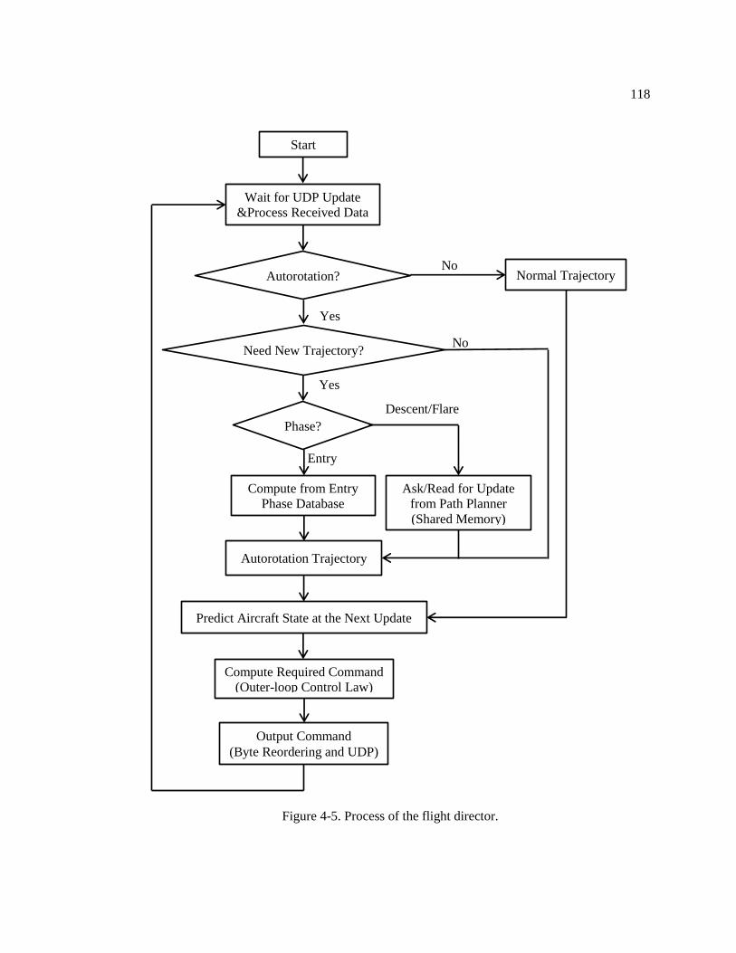
118
Figure 4-5. Process of the flight director.
Compute from Entry
Phase Database
Autorotation Trajectory
Autorotation?
Wait for UDP Update
&Process Received Data
Ask/Read for Update
from Path Planner
(Shared Memory)
Compute Required Command
(Outer-loop Control Law)
Need New Trajectory?
Output Command
(Byte Reordering and UDP)
Yes
Yes
Entry
Descent/Flare
No
Start
Phase?
Normal Trajectory
Predict Aircraft State at the Next Update
No

119
The flight director was designed to operate at the same normal simulation time step as the
cab interface. Every 0.05 seconds, the cab interface sends an update on the helicopter states to the
flight director and receives helicopter commands back through the UDP connection. To ensure
that the flight director could operate with the cab interface, the flight director process was
designed so that it would finish within 0.04 seconds.
The flight time was used to refer desired helicopter states in the trajectory. A time counter
was added to the primary flight control system in CSGE to generate the autorotation flight time
reference. The data exported from FLIGHTLAB included the aircraft’s roll and pitch attitude,
heading, velocity (in the body coordinate system), position (in the inertial coordinate system),
wind information (in inertial coordinate system), engine condition , and reference flight time.
[ ] (4.5)
The method used to transfer data between the flight director and the cab interface also
caused an inevitable delay in the helicopter command. As the current helicopter states and
commands are exchanged at the same time, the commands are generated based on the helicopter
states from the previous time step. A process of prediction was added to the flight director to
reduce the delay. The current helicopter states were used to approximate future helicopter states,
which would be compared against the future path command in order to generate helicopter
commands for the next 0.05 seconds.
Due to the time limit on the flight director process, the helicopter states at the next 0.05
seconds are predicted by simple integration equations:
{
| | | |
(4.6)
(4.7)

120
(
) (4.8)
( ) (4.9)
( ) (4.10)
where subscription k indicates the current time step and is the time difference between two
consecutive time steps ( ).
[
] [
] [
] (4.11)
The outer-loop control law was implemented to compute the helicopter commands from
the estimated helicopter states and path parameters at the next 0.05 second mark. Initially, the
control law for vertical axis was developed in the flight director process in the same way as those
of the other two axes. It was found that the collective commands given to the helicopter oscillated
severely, thereby causing instability and rapid rotor RPM drops to the helicopter. The fluctuation
in the collective commands may have arisen from the combination of high feedback gains in the
control law and the delay between the states and the commands. Further investigation found that
stability can be achieved by reducing the feedback gains; however, the control law would be
insensitive to the error on the vertical axis. To reduce the time delay in the control law, the outer-
loop vertical-axis control law was moved to the inner-loop control system in CSGE, which would
run at a faster rate than the fight director. The control law in CSGE is operated at the same time
step as that at which the simulation runs, and the control law experiences the least time delay
between the feedback states and the controls. The path commands for the vertical axis were sent
together with the roll and pitch commands and the reference time in order to generate the

121
collective command in CSGE. The output was sent to FLIGHTLAB with the command reference
time:
[ ] (4.12)
where the command time tag is
(4.13)
The vertical path following control law in FLIGHTLAB also estimates the change in path
commands within each update interval by:
(4.14)
(4.15)
where and are the estimated current path commands at the flight time
The network between the cab interface and the flight director was established in Linux-
Windows communication. These two operating systems have different ways of representing data
in the network. The bytes of the transferred data must be reordered to correspond with the
endianness of the destination. The data reordering process was done in the flight director. In the
case in which the network communication is lost, the controller in FLIGHTLAB was set to follow
the most recent update commands.
To the entry phase trajectory in the inertial coordinate system, the two-dimensional entry
phase solution would be found based on the initial airspeed. The solution would then be projected
in the inertial coordinate system according to the initial heading. Initially, this process for the
entry phase trajectory was applied to all initial airspeeds. However, in the very low initial
airspeed cases, the simulated flights showed a significant horizontal position and heading errors
even though significant control efforts were made. After engine failure, the helicopter suddenly
veered to the left. The change was made to reduce control efforts due to trajectory errors at the

122
beginning of the entry phase for the initial airspeed and hover cases. During the first second of the
entry phase autorotation from the initial airspeed below 10 ft/s, the outer-loop control law was
modified to receive no position error on both longitudinal and lateral axes. The trajectory solution
was re-connected to the flight one second after the engine failed. The trajectory at one second
after engine failure was synchronized to the aircraft position and projected in the direction that
the flight was headed.
4.3 Real-time Simulation Results
To assess the performance of the autonomous autorotation system, several autorotation
landings for a variety of initial conditions and helicopter weights were performed. Figure 4-6
shows the summarized results of the autonomous autorotation landings in real-time simulation.
These results pertain to nonlinear simulation models at three different gross weights. The
trajectory solutions were generated for the design gross weight (16,285 lbs) model, but
simulations at two heavier gross weights were performed in order to test robustness. The
simulations were performed for various steady level flight initial conditions.

123
Figure 4-6. Touchdown conditions of simulated autonomous autorotation flights.
In Figure 4-6, the touchdown conditions of the complete autorotation landing are
presented. The upper-left plot shows the touchdown position error. The touchdown locations are
mostly on the right and before the desired point. The upper-right plot shows the velocities at
touchdown. The maximum errors in the ground speed and lateral velocity are shown to be within
7 ft/s of the desired values. The lower-left plot shows the rotor speed and descent rate at
touchdown. The maximum descent rate at touchdown of the simulated flights is 15 ft/s, which is
incorporated with low rotor speed and is from the overweight condition. The lower-right plot
shows the roll attitude and heading error at touchdown. The maximum bank angle at touchdown
is 9º whereas the heading error is within 5º.
0 5 10 15 20-80
-60
-40
-20
0E
rror
in a
ppro
achin
g d
irection (
ft)
Lateral error (ft)
-5 0 5 1040
42
44
46
48
Gro
und s
peed (
ft/s
)
Lateral velocity (ft/s)
5 10 1518
20
22
24
26
Descent rate (ft/s)
(
rad/s
)
-10 -5 0-10
-5
0
5
(deg)
Headin
g e
rror
(deg)
16,285 lbs
17,914 lbs
19,542 lbs

124
Overall the results indicate the feasibility of the trajectory solutions for helicopters at
specified weights and the possibility of using trajectories generated for the lower-weight
helicopter for the higher-weight helicopter. However, the higher-weight helicopter had a higher
descent velocity at touchdown than did the lower-weight helicopter. In the higher-weight case,
the helicopter approached the landing point with a higher momentum, which required a higher
thrust force from the rotor in order to arrest the speed. For this higher thrust, more rotational
energy was consumed from the rotor, resulting in larger drop for rotor speed. The energy stored in
the rotor in this case might be insufficient, resulting in a touchdown with a higher descent speed,
a larger rotor speed drop and a higher error in the approaching direction (i.e., the heavier
helicopter deviates from the flare trajectory earlier than the lighter one does). A trend in regard to
the relationship between rotor speed and vertical speed at touchdown is also seen in the result:
The higher touchdown rotor speed usually corresponds to the lower vertical speeds at touchdown.
On average, the simulated flights landed one second before the desired time. The deviation of the
simulated landing touchdowns from the average point is less than 20 ft. The combination of the
lateral position error and lateral velocity might have caused a relatively high touchdown bank
angle.
Figure 4-7 through Figure 4-15 show examples of autonomous autorotation flights in
real-time simulation. Figure 4-7, Figure 4-10 and Figure 4-13 illustrate trajectory responses from
three selected cases of autorotation landing flights. The initial position is indicated by a red circle.
The target landing site is indicated by a blue square with a green arrow indicating the desired
landing direction. The connecting points between the phases are indicated by magenta circles.
The initial conditions (as well as the touchdown conditions) of the cases are given in Table 4-4.
Case 1 starts at a high-altitude hover. After engine failure, the helicopter gains forward speed by
following the entry phase trajectory and travels 5,831 ft northwest to the landing site located with
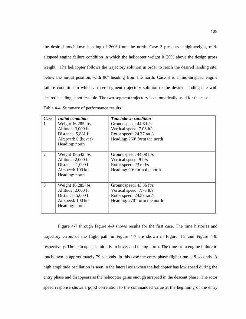
125
the desired touchdown heading of 260º from the north. Case 2 presents a high-weight, mid-
airspeed engine failure condition in which the helicopter weight is 20% above the design gross
weight. The helicopter follows the trajectory solution in order to reach the desired landing site,
below the initial position, with 90º heading from the north. Case 3 is a mid-airspeed engine
failure condition in which a three-segment trajectory solution to the desired landing site with
desired heading is not feasible. The two-segment trajectory is automatically used for the case.
Table 4-4. Summary of performance results
Case Initial condition Touchdown condition
1 Weight 16,285 lbs
Altitude: 3,000 ft
Distance: 5,831 ft
Airspeed: 0 (hover)
Heading: north
Groundspeed: 44.6 ft/s
Vertical speed: 7.03 ft/s
Rotor speed: 24.37 rad/s
Heading: 260º form the north
2 Weight 19,542 lbs
Altitude: 2,000 ft
Distance: 1,000 ft
Airspeed: 100 kts
Heading: north
Groundspeed: 44.08 ft/s
Vertical speed: 9 ft/s
Rotor speed: 23 rad/s
Heading: 90º form the north
3 Weight 16,285 lbs
Altitude: 2,000 ft
Distance: 5,000 ft
Airspeed: 100 kts
Heading: north
Groundspeed: 43.36 ft/s
Vertical speed: 7.76 ft/s
Rotor speed: 24.57 rad/s
Heading: 270º form the north
Figure 4-7 through Figure 4-9 shows results for the first case. The time histories and
trajectory errors of the flight path in Figure 4-7 are shown in Figure 4-8 and Figure 4-9,
respectively. The helicopter is initially in hover and facing north. The time from engine failure to
touchdown is approximately 79 seconds. In this case the entry phase flight time is 9 seconds. A
high amplitude oscillation is seen in the lateral axis when the helicopter has low speed during the
entry phase and disappears as the helicopter gains enough airspeed in the descent phase. The rotor
speed response shows a good correlation to the commanded value at the beginning of the entry
126
phase but drops suddenly in the middle of the entry phase. The rotor speed then slowly recovers
during the descent phase until it reaches its stable point over the commanded value. A good
correlation of rotor speed response and command is shown in the later descent phase and flare
phase to the touchdown.
Figure 4-10 through Figure 4-12 show results for the second case. The time histories and
trajectory errors of the flight path in Figure 4-10 are shown in Figure 4-11 and Figure 4-12,
respectively. The helicopter is initially in a straight and level flight heading north with an airspeed
of 100 kts. The helicopter gross weight is 19,542 lbs, whereas the trajectory-generating algorithm
generates a solution for the helicopter with a gross weight of 16,285 lbs. The landing site is close
to the point of engine failure; however, the helicopter must execute a long turn to reach the site.
The time from engine failure to touchdown is approximately 64 seconds. The pitch attitude
response shows an error of -10º during the first turning segment of the descent phase. The rotor
speed response is well over the commanded value from the entry phase trajectory. It slowly drops
when the helicopter enters the descent phase, and it operates under the commanded value
throughout the descent phase.
Figure 4-13 through Figure 4-15 show results for the third case. The time histories and
trajectory errors of the flight path in Figure 4-13 are shown in Figure 4-14 and Figure 4-15,
respectively. The helicopter is initially at the same condition as the second case except that in
Case 3 the helicopter weight is at its design value. The landing site is 5,000 ft away to the east,
and the desired touchdown heading is to the west. The best three-segment trajectory to the
landing site is a low RPM, RSR type path which turns the helicopter to the east and then makes a
U-turn to approach the site; however, the trajectory requires more altitude than is available. This
algorithm indicates that the three-turn trajectory solution is not feasible. The two-segment
trajectory is automatically considered and implemented as the trajectory solution. The time from
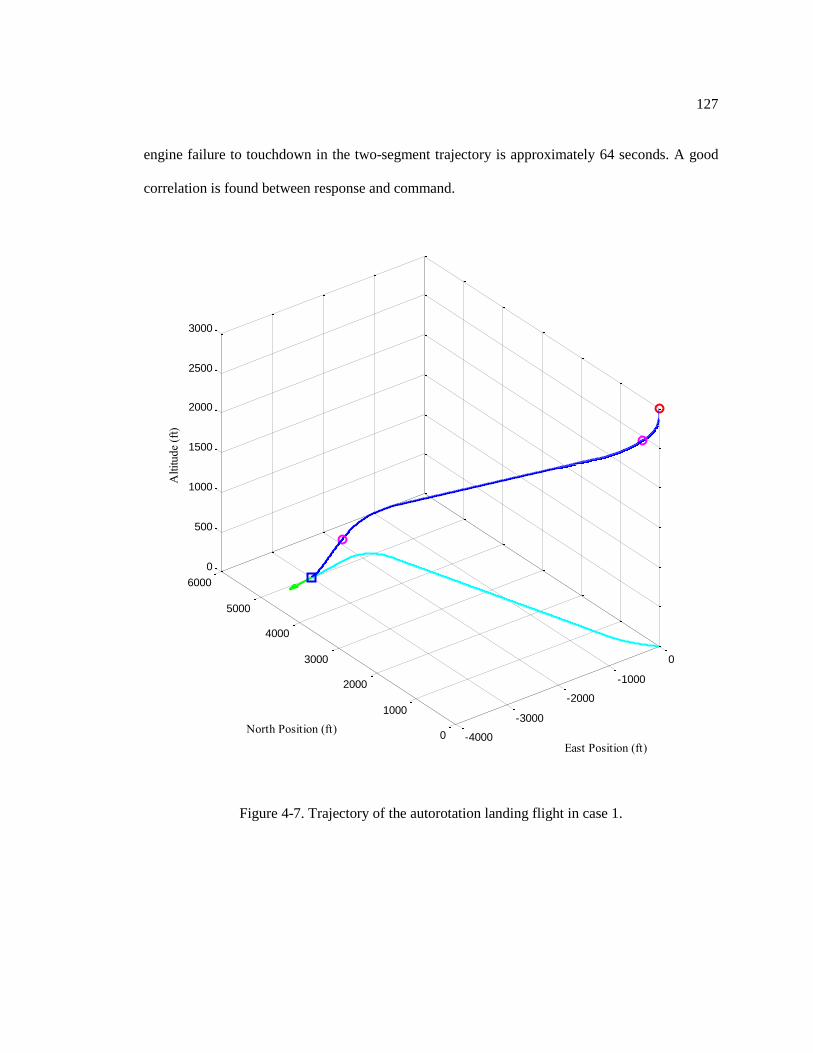
127
engine failure to touchdown in the two-segment trajectory is approximately 64 seconds. A good
correlation is found between response and command.
Figure 4-7. Trajectory of the autorotation landing flight in case 1.
-4000
-3000
-2000
-1000
0
0
1000
2000
3000
4000
5000
6000
0
500
1000
1500
2000
2500
3000
East Position (ft)
North Position (ft)
Altitude
(ft)

128
Figure 4-8. Time histories of the autorotation landing flight in case 1.
0 10 20 30 40 50 60 70 800
50
100
Vel
oci
ty (
ft/s
)
0 10 20 30 40 50 60 70 800
1000
2000
3000
Altitude
(ft)
0 10 20 30 40 50 60 70 800
20406080
Des
cent ra
te (
ft/s
)
0 10 20 30 40 50 60 70 80-180
0
180
Hea
din
g (
deg
)
0 10 20 30 40 50 60 70 80-45
0
45
(d
eg)
0 10 20 30 40 50 60 70 80-40-20
02040
(
deg
)
0 10 20 30 40 50 60 70 8018
24
30
(
rad/s
)
time (s)
Response
Command

129
Figure 4-9. Deviations in the trajectory of the autorotation landing flight in case 1.
0 10 20 30 40 50 60 70 80
-20-10
01020
Longitudin
al e
rror
(ft)
0 10 20 30 40 50 60 70 80-30
-15
0
15
30
Lat
eral
dev
iation (
ft)
0 10 20 30 40 50 60 70 80-10
0
10
Altitude
erro
r (f
t)
0 10 20 30 40 50 60 70 80-20
-10
0
10
20
Forw
ard s
pee
d e
rror
(ft/s)
0 10 20 30 40 50 60 70 80-40
-20
0
20
40
Lat
eral
spee
d (
ft/s
)
0 10 20 30 40 50 60 70 80-10
0
10
Des
cent ra
te e
rror
(ft/s)
time (s)

130
Figure 4-10. Trajectory of the autorotation landing flight in case 2.
-2000
-1500
-1000
-500
0
500
1000
1500
-500
0
500
1000
1500
2000
0
200
400
600
800
1000
1200
1400
1600
1800
2000
East Position (ft)North Position (ft)
Altitude
(ft)

131
Figure 4-11. Time histories of the autorotation landing flight in case 2.
0 10 20 30 40 50 60 700
100
200
Vel
oci
ty (
ft/s
)
0 10 20 30 40 50 60 700
1000
2000
Altitude
(ft)
0 10 20 30 40 50 60 700
25
50
Des
cent ra
te (
ft/s
)
0 10 20 30 40 50 60 70-270
-180
-90
0
Hea
din
g (
deg
)
0 10 20 30 40 50 60 70-45
0
45
(d
eg)
0 10 20 30 40 50 60 70
0
20
40
(
deg
)
0 10 20 30 40 50 60 7018
24
30
(
rad/s
)
time (s)
Response
Command

132
Figure 4-12. Deviations in the trajectory of the autorotation landing flight in case 2.
0 10 20 30 40 50 60 70
-20-10
01020
Longitudin
al e
rror
(ft)
0 10 20 30 40 50 60 70-15
0
15
Lat
eral
dev
iation (
ft)
0 10 20 30 40 50 60 70-10
0
10
Altitude
erro
r (f
t)
0 10 20 30 40 50 60 70-20
-10
0
10
20
Forw
ard s
pee
d e
rror
(ft/s)
0 10 20 30 40 50 60 70-40
-20
0
20
40
Lat
eral
spee
d (
ft/s
)
0 10 20 30 40 50 60 70-10
0
10
Des
cent ra
te e
rror
(ft/s)
time (s)
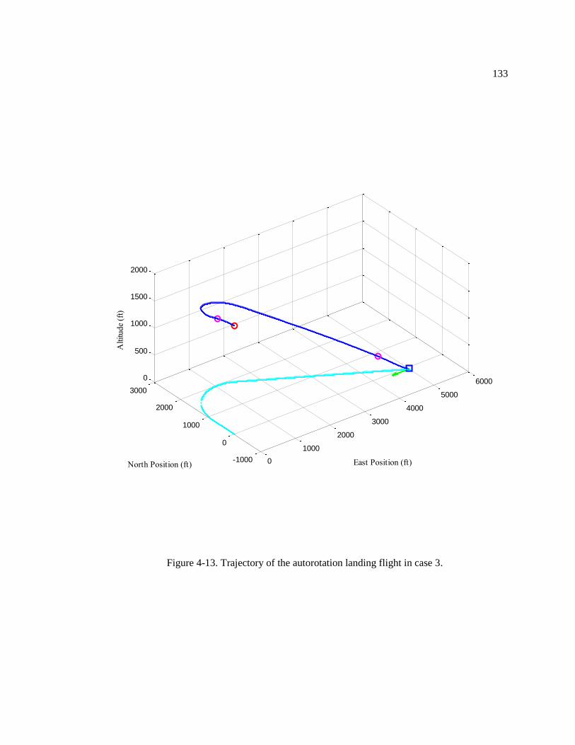
133
Figure 4-13. Trajectory of the autorotation landing flight in case 3.
0
1000
2000
3000
4000
5000
6000
-1000
0
1000
2000
3000
0
500
1000
1500
2000
East Position (ft)North Position (ft)
Altitude
(ft)

134
Figure 4-14. Time histories of the autorotation landing flight in case 3.
0 10 20 30 40 50 60 700
100
200
Vel
oci
ty (
ft/s
)
0 10 20 30 40 50 60 700
1000
2000
Altitude
(ft)
0 10 20 30 40 50 60 700
25
50
Des
cent ra
te (
ft/s
)
0 10 20 30 40 50 60 70
0
90
180
Hea
din
g (
deg
)
0 10 20 30 40 50 60 70-45
0
45
(d
eg)
0 10 20 30 40 50 60 70
0
20
40
(
deg
)
0 10 20 30 40 50 60 7018
24
30
(
rad/s
)
time (s)
Response
Command
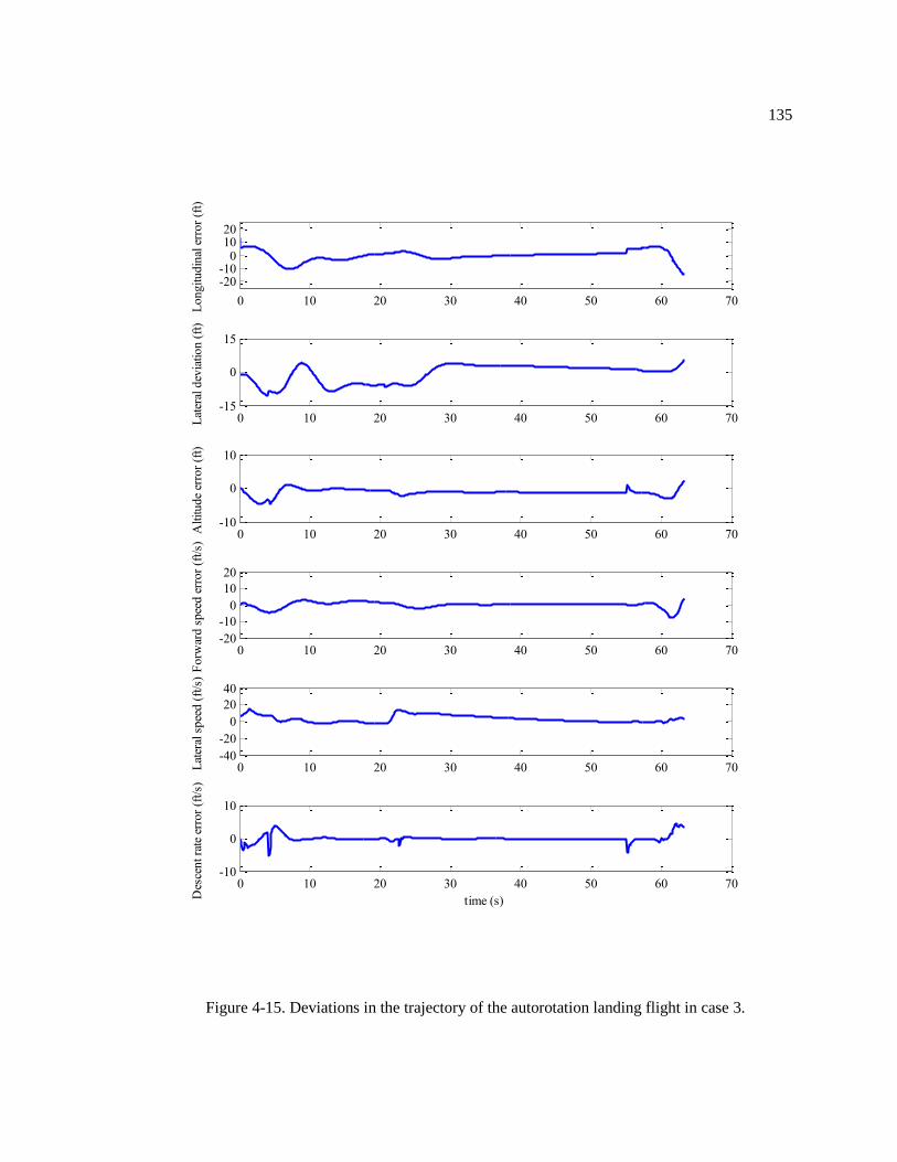
135
Figure 4-15. Deviations in the trajectory of the autorotation landing flight in case 3.
0 10 20 30 40 50 60 70
-20-10
01020
Longitudin
al e
rror
(ft)
0 10 20 30 40 50 60 70-15
0
15
Lat
eral
dev
iation (
ft)
0 10 20 30 40 50 60 70-10
0
10
Altitude
erro
r (f
t)
0 10 20 30 40 50 60 70-20
-10
0
10
20
Forw
ard s
pee
d e
rror
(ft/s)
0 10 20 30 40 50 60 70-40
-20
0
20
40
Lat
eral
spee
d (
ft/s
)
0 10 20 30 40 50 60 70-10
0
10
Des
cent ra
te e
rror
(ft/s)
time (s)
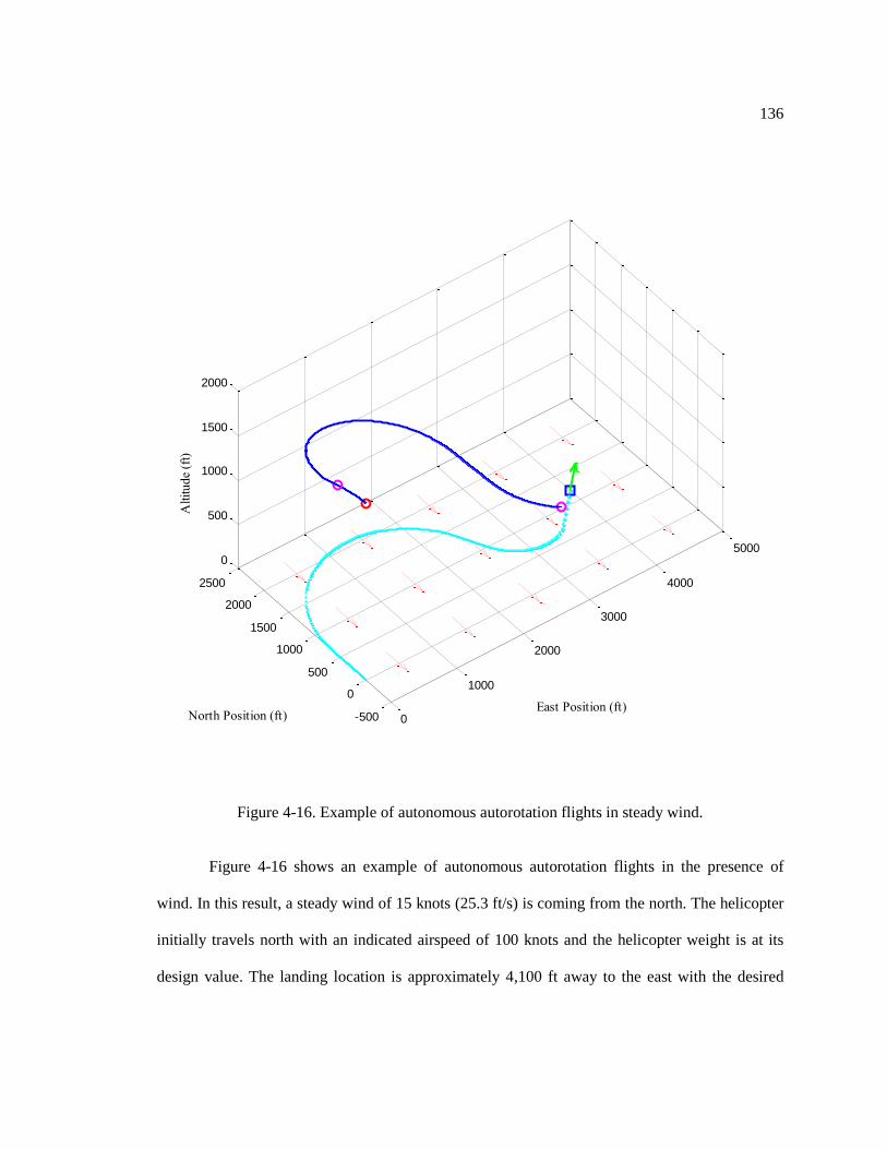
136
Figure 4-16. Example of autonomous autorotation flights in steady wind.
Figure 4-16 shows an example of autonomous autorotation flights in the presence of
wind. In this result, a steady wind of 15 knots (25.3 ft/s) is coming from the north. The helicopter
initially travels north with an indicated airspeed of 100 knots and the helicopter weight is at its
design value. The landing location is approximately 4,100 ft away to the east with the desired
0
1000
2000
3000
4000
5000
-500
0
500
1000
1500
2000
2500
0
500
1000
1500
2000
East Position (ft)North Position (ft)
Altitude
(ft)

137
touchdown heading of 45º from the north. The flare phase flight is not included in the result due
to the experience of cross wind, which is not accounted for in the present work.
Figure 4-17 shows the time histories of the rotor flapping angles and the rotorcraft
attitude responses during an autonomous autorotation landing flight. These flapping angles define
the orientation of the rotor tip path plane and are measured relative to the rotor hub orientation.
The details of the rotor flapping responses during the flare phase from Figure 4-17 are shown in
Figure 4-18. The result shows the minimum flapping angle of -7º ( ) at the back of the
rotor and -11º ( ) at the front of the rotor during the flare phase and at touchdown,
respectively. The drop in the coning angle, , is seen at the connecting points between the
segments. This coning angle drop is mainly due to the discontinuity of the descent velocity at the
connecting points. The minimum flapping angle at the back of the rotor is due to an attempt to
pitch up to decelerate airspeed during the flare, whereas the minimum flapping angle at the front
of the rotor is due to an attempt to return from the high pitch attitude flare to the zero pitch
attitude at touchdown. The rotor module of the generic utility helicopter is mounted to the top of
the fuselage with a built-in 3º forward tilt. This built-in forward tilt of the main rotor system
reduces the risk of the main rotor blade striking the tail boom during the high pitch-attitude flare.
Based on an estimation of the tail boom dimension in the principal dimensions of the helicopter in
Figure 2-2, the minimum flapping angle at the back of the rotor before the main rotor hits the tail
boom is -15º and the minimum flapping angle at the front of the rotor before the main rotor
makes a ground contact is -24º at touchdown. The rotor flapping responses in autonomous
autorotation flights are well within this estimated bound and indicate neither ground contact nor
tail boom strike by the main rotor.
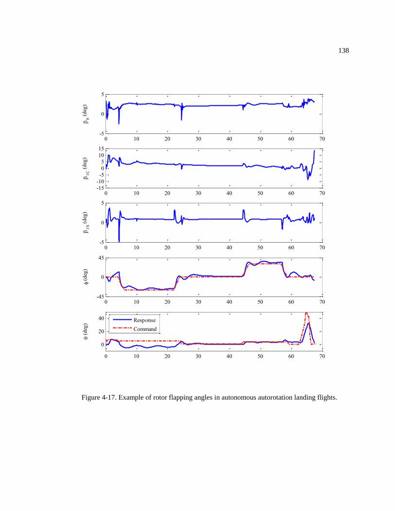
138
Figure 4-17. Example of rotor flapping angles in autonomous autorotation landing flights.
0 10 20 30 40 50 60 70-5
0
5
0 (
deg
)
0 10 20 30 40 50 60 70-15
-10
-5
0
5
10
15
1
C (
deg
)
0 10 20 30 40 50 60 70-5
0
5
1
S (
deg
)
0 10 20 30 40 50 60 70-45
0
45
(d
eg)
0 10 20 30 40 50 60 70
0
20
40
(
deg
)
Response
Command

139
Figure 4-18. Example of rotor flapping angles during flare-phase autorotation.
59 60 61 62 63 64 65 66 670
1
2
3
4
5
0 (
deg
)
59 60 61 62 63 64 65 66 67-15
-5
5
15
1
C (
deg
)
59 60 61 62 63 64 65 66 67-5
0
5
1
S (
deg
)
59 60 61 62 63 64 65 66 67-15
0
15
(d
eg)
59 60 61 62 63 64 65 66 67
0
20
40
(
deg
)
Response
Command

140
Figure 4-19. Computation time for the descent-phase trajectory.
Figure 4-19 is a histogram showing the time required to compute the descent-phase
trajectory in several cases. It was found that the average time to compute the descent-phase
trajectory was 2.1 seconds and 89% of the descent phase trajectories were computed within 4
seconds. Note that the initial conditions in this evaluation were generated randomly. The results
also include cases for which there were no trajectory solutions to the desired landing site. The
algorithm might require more than 4 seconds due to these “no trajectory solution” cases.
4.4 Discussion
The autonomous autorotation system shows adequate results in the real-time simulated
autorotation landings. Successful autorotation landings were obtained from most of the attempts
at the design gross weight when the actual helicopter weight matched the weight used in the
trajectory calculations. The chance of a successful autorotation landing was found to decrease as
the actual helicopter weight was higher than the trajectory referred weight.
1 2 3 4 5 6 7 80
20
40
60
80
100
Time required to compute descent-phase path(sec)
Count

141
The compensation for the approximation error in the autorotation descent velocity
approximation function showed an observable effect in the rotor speed responses from simulated
autorotation flights. Due to the compensation, the rotorcraft would have a sink rate in the
trajectory higher than the required sink rate for the trajectory-commanded rotor speed. As the
rotorcraft was commanded to follow the trajectory, the operating autorotation rotor speed would
be higher than the commanded value. By following the trajectory, the rotor speed response would
be increased until the operating rotor speed was achieved.
With additional gross weight, the quasi-steady state autorotation performance was
improved in the high-speed region but was declined in the low-speed autorotation. It was found
that, for the same rotor RPM, the heavier gross weight helicopter required a lower descent rate for
autorotation in the high airspeed region whereas it required a higher descent rate for autorotation
in the low airspeed region. The evidence can be inferred from the rotor speed response in Figure
4-11. The effect of extra gross weight on the entry phase and the flare phase was also observed.
The entry trajectory, which brought the lighter-weight helicopter from hover, led the heavier
helicopter to a crash landing due to a higher drop in rotor speed. For the cases that the heavier-
weight helicopters were able to follow the generated trajectory until the flare phase, the flare
trajectory results show a higher descent rate at touchdown.
Incomplete landings (crashes) were normally found when the rotor speed dropped below
a recovery point during the autorotation flight. The rotor speed of 21 rad/s (78% RPM) was
approximated as the recovery point for the nonlinear helicopter simulation model. Incomplete
landings were mostly found in trajectory solutions that incorporated one or more of these
maneuvers: (1) high bank angle, low speed turn (30º bank angle and airspeed below 90 ft/s), (2)
high bank angle, very high speed turn (30º bank angle and airspeed above 230 ft/s), and (3) low
airspeed, accelerating turn.

142
At the connecting points of phases and segments in the analytical trajectory, the rotor was
designed to leave the previous quasi-steady autorotation state and shortly enter the next quasi-
steady autorotation state. This change in autorotation state does not occur immediately with the
complete helicopter dynamics. As the rotor leaves one autorotation state, the rotor keeps losing
rotational energy, resulting in a rotor speed drop, until it arrives at the next autorotation state.
Large control effort in this transition state tends to deplete more rotor rotational energy and can
possibly cause the rotor speed to drop below the recovery point. It was found that the magnitude
of the rotor speed drop usually varied as follows: (1) the deviation in vertical velocity, (2) the
forward speed at connecting points of phases and segments, and (3) the helicopter’s gross weight.
A higher vertical speed deviation, lower forward velocity, and higher gross weight gave a larger
rotor speed drop at the connecting point.
A low-speed turn at a high bank angle is usually associated with a high descent rate,
which requires a high degree of control effort during the transition. A very high-speed turn at a
high bank angle creates an overshoot of the helicopter response from the commanded trajectory.
A high degree of control effort is required to recover from the overshoot. An accelerating turn at
low airspeed shows a high oscillation along the longitudinal and lateral axes of the helicopter.
The attempt to control the helicopter results in very high control efforts during the path.
The other main cause of incomplete landings was the delay in descent phase trajectory
computation. Even though, the flight director would keep the last updated attitude command to
keep the helicopter in an autorotation state, the deviation between the trajectory and the current
position was mostly too high and beyond the recovery point when the descent trajectory was
executed. Note that this delay in the descent phase trajectory computation is mainly due to the
implementation on non-optimized hardware and software. However, the trajectory computation
time must be verified and set appropriately for the operating environment.

143
To increase the robustness of the trajectory-generating method, a cost function, which
penalizes undesired maneuvers, can be added to Eq. (2.104). A nonlinear inequality constraint
function can also be formulated for the optimizer to prevent undesired maneuvers in the trajectory
solution. The computation time can easily be increased; however, reachable descent gliding
distance would suffer from longer time duration in the entry phase as there is less altitude
available in the descent phase.
The path following control law shows adequate performance in controlling the helicopter
in most of all the three phases. The helicopter presented high oscillations in the lateral and
directional axes while performing autorotation in the low-speed region and in the accelerating
trajectories. This oscillation might be due to one or a combination of (1) the lateral-directional
cross coupling effect, which induced an oscillation in one axis to the other, (2) the instability of
autorotation at low airspeed, or (3) improper design of the outer-loop control law. Further study
would be required to verify the cause.
The rotor flapping responses show a large movement of the longitudinal flapping angle
during the flare-phase autorotation. The negative longitudinal flapping angle indicates an attempt
to pitch up the helicopter, whereas the positive longitudinal flapping angle indicates an attempt to
pitch the helicopter down. In this work, the simulation result shows that the rotor’s flapping
responses are within safe operating range during the autonomous autorotation landings. But the
flapping responses can differ due to a change in the rotor system, the primary flight control
(inner-loop control), and the path following control (outer-loop control). It is suggested that the
flapping responses must be monitored closely when the autonomous autorotation system is
implemented in order to ensure the safe autorotation landings.

Chapter 5
Implementation and Preliminary Result on Helicopter UAV
This chapter presents an early phase of the implementation of the autonomous
autorotation landing for an unmanned helicopter. The autorotation path planning algorithms
developed in Chapter 2 is implemented to provide autonomous autorotation landing trajectories
for the Hornet Mini UAS. The simulation software of the UAS is used to test the trajectories
generated by the autorotation trajectory generating algorithms in order to evaluate the feasibility
of using them in the actual helicopter UAS. Detail of the autorotation trajectory algorithm
implementation is described. Finally, preliminary results from simulation are presented.
5.1 Hornet Mini Helicopter UAV
The Hornet Mini UAS is a small scale, 55-inch rotor diameter unmanned helicopter
designed by Adaptive Flight Incorporated. The properties of this helicopter are shown in Table
5-1. The Hornet Mini is an autonomous UAV that can be operated in both user-controlled manual
mode and autonomous waypoint flight. In both cases the user interfaces with the ground control
station (GCS). The UAS package also includes a flight simulator which can be used for
integration testing and for operator training.
In the standard waypoint command mode, the waypoints given to the vehicle through the
ground control station are used by a built-in trajectory generator in the vehicle’s on-board
computer to generate a flight path based on waypoints and command the vehicle to follow the
self-generated trajectory.

145
Figure 5-1. Adaptive Flight’s Hornet Mini UAS [90]
Table 5-1. Properties of Hornet Mini UAS
Description Value
Aircraft
Normal weight (lbf)
11.58
Main rotor: Teetering rotor
number of blades
nominal speed (rad/s)
radius (ft)
2
188.5
2.292
Tail rotor:
number of blades
nominal speed (rad/s)
radius (ft)
2
979
0.375
Control surface range: [min, max]
main rotor lateral cyclic (rad)
main rotor longitudinal cyclic (rad)
main rotor collective (rad)
tail rotor collective (rad)
[-0.12, 0.12]
[-0.12, 0.12]
[-0.065, 0.17]
[-0.183, 0.332]

146
5.2 Implementation for UAS Simulation
Figure 5-2 illustrates the initial design of the autonomous autorotation system
implementation on the UAV. The information on aircraft conditions is obtained from the Hornet
Mini ground control station and is used as the initial conditions for the autorotation trajectory
algorithms. The algorithm uses measured information of the initial condition at engine failure
(velocity, position and heading) and a pre-determined terminal condition at touchdown (location
and heading) to generate a feasible autorotation trajectory. The algorithms were used to calculate
complete autorotation trajectory solutions, and the trajectories were used to command
autorotation flights in the Hornet Mini UAS simulation through waypoints. Each waypoint
contains information on position, velocity, acceleration, and heading at that point in the
autorotation trajectory. The generated command waypoints are given to the vehicle through the
ground control station. The built-in system onboard the UAV uses the waypoints to regenerate the
trajectory using its own built-in trajectory generator. Finally, the UAV is commanded to follow
the regenerated trajectory via the existing inner and outer loop control on the UAV system.
Because the autorotation trajectory solutions are converted to waypoints, and then converted back
to a continuous trajectory by the Hornet Mini autopilot’s trajectory generator, there can be slight
differences in the final commanded trajectory.
The present work implements only the autorotation trajectory algorithms presented in
Chapter 2 to generate the trajectory solution from the specified engine failure points to the
predetermined landing locations for the UAV. The control law presented in Chapter 3 is not
applied since the autonomous control on the UAV is achieved using the built-in system.

147
Figure 5-2. Schematic of autonomous autorotation system implementation on UAS system
The data of autorotation operating points were extracted from the simulation software to
tune the point mass model. The drag coefficient parameter, , in Eq. (2.10) was tuned so that the
point mass model descent rate matched that of the Hornet Mini simulation in several steady-state
autorotation conditions. It was found that approximating the profile drag coefficient by a linear
function of the rotor speed resulted in reasonable correlation.
(5.1)
where are approximation constants obtained from a least square method. The limits
are used to constrain the value and ensure reasonable autorotation predictions.
Figure 5-3 shows the correlation between the descent rate of the Hornet Mini simulation
model and that of the tuned point mass model at various autorotation operating conditions. Data
points in the figure correspond to autorotation operating conditions at airspeed between 15 and 40
ft/s, rotor speed between 113 and 207 rad/s (60% to 110% RPM) and bank angle between 0 and
20 deg.
Trajectory
Solution
Vehicle &
Wind
Conditions
Waypoint
Command
Vehicle
Conditions
Control/
Ground
Station
RC
Helicopter
UAV System Autonomous Autorotation System
Autorotation
Flight
Director
Path
Planner
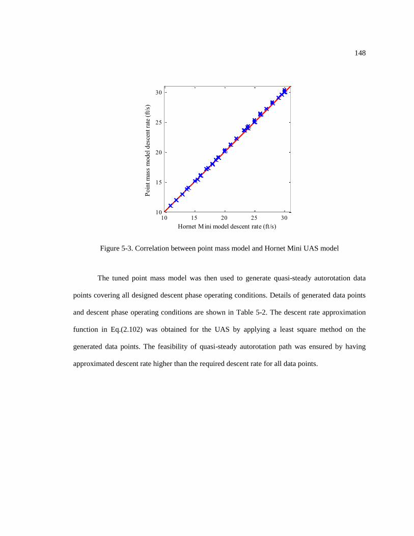
148
Figure 5-3. Correlation between point mass model and Hornet Mini UAS model
The tuned point mass model was then used to generate quasi-steady autorotation data
points covering all designed descent phase operating conditions. Details of generated data points
and descent phase operating conditions are shown in Table 5-2. The descent rate approximation
function in Eq.(2.102) was obtained for the UAS by applying a least square method on the
generated data points. The feasibility of quasi-steady autorotation path was ensured by having
approximated descent rate higher than the required descent rate for all data points.
10 15 20 25 3010
15
20
25
30
Po
int m
ass
mo
del
des
cen
t ra
te (
ft/s
)
Hornet Mini model descent rate (ft/s)
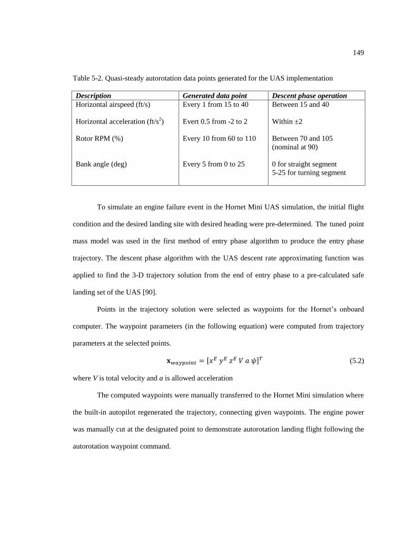
149
Table 5-2. Quasi-steady autorotation data points generated for the UAS implementation
Description Generated data point Descent phase operation
Horizontal airspeed (ft/s)
Every 1 from 15 to 40 Between 15 and 40
Horizontal acceleration (ft/s2)
Evert 0.5 from -2 to 2
Within ±2
Rotor RPM (%)
Bank angle (deg)
Every 10 from 60 to 110
Every 5 from 0 to 25
Between 70 and 105
(nominal at 90)
0 for straight segment
5-25 for turning segment
To simulate an engine failure event in the Hornet Mini UAS simulation, the initial flight
condition and the desired landing site with desired heading were pre-determined. The tuned point
mass model was used in the first method of entry phase algorithm to produce the entry phase
trajectory. The descent phase algorithm with the UAS descent rate approximating function was
applied to find the 3-D trajectory solution from the end of entry phase to a pre-calculated safe
landing set of the UAS [90].
Points in the trajectory solution were selected as waypoints for the Hornet’s onboard
computer. The waypoint parameters (in the following equation) were computed from trajectory
parameters at the selected points.
[ ] (5.2)
where V is total velocity and a is allowed acceleration
The computed waypoints were manually transferred to the Hornet Mini simulation where
the built-in autopilot regenerated the trajectory, connecting given waypoints. The engine power
was manually cut at the designated point to demonstrate autorotation landing flight following the
autorotation waypoint command.

150
5.3 Preliminary Simulation Results
Several cases of varying distance to touchdown point and initial speed were tested to
examine performance of the autorotation trajectory algorithms. Results (Initial conditions as well
as touchdown conditions) of two representative cases are presented in Table 5-3. In the first case,
the UAS was required to travel a long distance with low rotor speed to achieve the desired
landing location and heading. The landing site was located 450.7 ft to the east, but the desired
heading at landing was to the west. The vehicle was required to turn to the east first and then
make a U-turn to attain the desired heading at the flare initiation point. In the second case, the
autorotation trajectory distance to the landing site was shorter than that of the first case. The UAS
could travel with a rotor speed near the nominal rotor speed for autorotation (90%RPM).
Table 5-3. Summary of results from representative cases
Case Initial condition Touchdown condition Touchdown error
1 Altitude: 360 ft
Distance: 450.7 ft
Airspeed: 30 ft/s
Heading: 30º N
Groundspeed: 7.7 ft/s
Vertical speed: 12.4 ft/s
Rotor speed: 84 rad/s
6º bank angle (0º desired)
10º pitch angle (0º desired)
24º heading
2.2 ft from desired point
2 Altitude: 375 ft
Distance: 457.5 ft
Airspeed: 25 ft/s
Heading: 30º N
Groundspeed: 15.67 ft/s
Vertical speed: 9.8 ft/s
Rotor speed: 100 rad/s
3º bank angle (0º desired)
13.8º pitch angle (0º desired)
4.7º heading
3.7 ft from desired point
Figure 5-4 and Figure 5-5 show results for Case 1. Figure 5-4 shows the waypoint
command and autopilot-generated trajectory in the ground control station interface. Time
histories of the trajectory solution and simulated flight are shown in Figure 5-5. The time from
engine failure to touchdown is approximately 26.5 seconds (entry: 4 sec, descent: 20.5 sec and
flare: 2 sec).

151
Figure 5-6 and Figure 5-7 show results for Case 2. Figure 5-6 shows the waypoint
command and autopilot-generated trajectory in the ground control station interface. Time
histories of the trajectory solution and simulated flight are shown in Figure 5-7. The simulated
autorotation landing flight took approximately 20.7 seconds which was 0.5 seconds shorter than
the trajectory solution.
Overall simulation results show the feasibility of the algorithms for performing
autonomous autorotation landing with the Hornet Mini UAS. The simulated flights from standard
waypoint control showed some difficulty in following the generated trajectory solutions,
especially during the entry and flare phases, which required relatively abrupt maneuvers.
Touchdown velocities of the two simulated flights are higher than the target touchdown velocities
of 4.3 ft/s ground speed and 5.5 ft/s descent rate. These relatively high touchdown velocities
could be due to the fact that the simulated flight did not follow the trajectory solution well in the
flare phase. The difference between the simulated flight and the trajectory solution might be due
to the setup of waypoint commands which assigns the total velocity at each waypoint rather than
horizontal speed and descent velocity independently. For descent phase, the standard waypoint
control worked reasonably well for autorotation trajectory flights. Incomplete landing flights
(crash) were sometimes observed in simulated flight tests due to the built-in autopilot which
slowed down the airspeed of UAS during the autorotation.

152
Figure 5-4. Flight path of autorotation landing flight in ground control station interface for case 1

153
Figure 5-5. Response and trajectory control histories for case 1
0 5 10 15 20 25 30-30
-15
0
15
30
(d
eg)
0 5 10 15 20 25 30-20
0
20
(
deg
)
0 5 10 15 20 25 300
90
180
270
360
(
deg
)
0 5 10 15 20 25 3080
150
220
(
rad/s
)
0 5 10 15 20 25 300
200
400
Altitude
(ft)
0 5 10 15 20 25 300
20
40
Vel
oci
ty (
ft/s
)
0 5 10 15 20 25 305
15
25
Des
cent ra
te (
ft/s
)
time (s)
Response
Trajectory

154
Figure 5-6. Flight path of autorotation landing flight in ground control station interface for case 2

155
Figure 5-7. Response and trajectory control histories for case 2
0 2 4 6 8 10 12 14 16 18 20 22-10
0
10
20
(d
eg)
0 2 4 6 8 10 12 14 16 18 20 22-20
0
20
(
deg
)
0 2 4 6 8 10 12 14 16 18 20 220
45
90
135
180
(
deg
)
0 2 4 6 8 10 12 14 16 18 20 2280
150
220
(
rad
/s)
0 2 4 6 8 10 12 14 16 18 20 220
200
400
Altitu
de
(ft)
0 2 4 6 8 10 12 14 16 18 20 220
20
40
Vel
oci
ty (
ft/s
)
0 2 4 6 8 10 12 14 16 18 20 225
15
25
Des
cen
t ra
te (
ft/s
)
time (s)
Response
Trajectory
Chapter 6
Conclusions and Future work
This dissertation has described a method for end-to-end control of autonomous helicopter
autorotation. The method is capable of responding the engine power loss situation in real time and
creating three-dimensional autorotation trajectory in the presence of wind. The objective of the
method is to autonomously guide the helicopter from the moment of engine failure to safe landing
at a specified touchdown point. The system includes an inner loop flight controller to stabilize the
vehicle and follow a desired trajectory and a trajectory generator that computes safe, dynamically
feasible trajectories to the desired touchdown point. The trajectory planner divides flight into
three phases: entry, which brings the helicopter from engine failure to a steady descent condition;
descent, which guides the helicopter to a state from which flare can be safely initiated; and flare,
which guides the helicopter to safe landing. The inner loop flight controller uses dynamic
inversion and model following control to stabilize the vehicle. An outer loop trajectory following
controller also uses dynamic inversion control scheme to track trajectory commands.
6.1 Conclusions
Simulation testing shows that the autonomous autorotation system is able to provide
successful autorotation landings for the FLIGHLAB simulation model of a generic utility
helicopter. For the helicopter with design gross weight, the system resulted in autonomous
autorotation landings touchdown with sink rate lower than 8 ft/s and horizontal airspeed lower
than 47 ft/s. The heading error at touchdown was within 7º from the desired heading. The position
error at touchdown was within 60 ft from the desired landing point. The average touchdown

157
points were 25 ft in front of and 10 ft to the right of the desired landing point. All touchdown
points were scattered within a 25 ft radius from this average point.
The descent-phase trajectory algorithm can compute 89% of autorotation cases within 4
seconds in a standard commercial PC with 2.81GHz dual core processor. The average time
required to compute a descent-phase trajectory is 2.1 seconds. The maximum time required to
compute a descent-phase trajectory is found at 7.6 seconds.
The tuned point mass model adequately represents autorotation performance in
autorotation trajectory generation. The developed trajectory generating algorithms are capable of
generating trajectory solutions which the helicopter can follow in autorotation flights. The
generated trajectory solution is sensitive to the helicopter weight. It is possible that the trajectory
can be followed by the helicopter with heavier weight but the touchdown condition will be at a
higher descent rate.
The trajectory generating method allows deviation in vertical velocity at the segment
connecting points. This deviation creates a rotor speed drop in the rotor response through the high
control efforts in an attempt to reduce trajectory error. At some connecting points, the trajectory
requires the rotor to generate a downward force which reduces the rotor coning angle. The cost
function in descent phase algorithm can be modified to reduce this deviation in vertical speed at
the connecting points.
Robustness of the autonomous autorotation method can be obtained in bounded operating
regions of horizontal velocity, acceleration, bank angle, and helicopter gross weight. Further
study is required in order to find the quantitative data of these bounded regions.
The developed autorotation trajectory generating method can be applied to different size
of helicopter. The preliminary results in Hornet Mini UAS simulation indicate the feasibility of
the algorithms for performing autonomous autorotation landing with the Hornet Mini UAS. Some

158
difficulties in achieving accurate path following in the final flare phase using a standard waypoint
control law are observed.
6.2 Future Work
The future work could be in two categories; further study in autonomous autorotation
landing and improvement of autonomous autorotation system. The next step of autonomous
autorotation landing study would be the implementation on an actual hardware system.
Preliminary simulation results on Hornet Mini UAS demonstrate feasibility of autorotation
trajectory generated from the three autorotation phase trajectory algorithms. An alternative UAS
control, which receives continuous external trajectory command, would be needed to replace the
standard waypoint-controlled trajectory, which strictly limits the maneuvers on the UAS. More
simulated flight tests would be required to ensure the feasibility of generated trajectories and the
performance of the new control method on the UAS.
For the improvement of autonomous autorotation system, the following topics could be
considered:
The descent phase algorithm could be incorporated with obstacle avoidance features.
Information on obstacle (e.g. buildings, trees, restricted area) could be used to formulate
additional cost function, which penalizes trajectories near the obstacles, in the descent phase cost
function. The disadvantage of this feature would be the longer time required to generate a
trajectory solution since more computation is added in the descent phase trajectory algorithm.
The computation time of descent phase trajectory generation could be reduced by
eliminating unnecessary computation of path types which are not likely to be the solution for the
situation. The information on initial altitude, airspeed, and wind could be combined with the
distance and direction to the landing site, and desired touchdown heading to determine the

159
probability of each path type (RSR, RSL, LSL, LSR, RS, and LS) to be the solution prior to the
trajectory computation. For example, in the situation that the landing site is relatively far away to
the right, it is obvious the best solution would make a right turn in the first turning segment.
Therefore, the solution with LSL, LSR, or LS path types would likely be a bad solution and
would be unneeded to compute.
To have the autonomous autorotation system running as a real-time application in actual
helicopter hardware, the development of an optimizer suitable to find the parametric control
variables for the descent phase trajectory would be required. This would enable the transition of
autonomous autorotation system to other programming languages which are more capable of real-
time operation (e.g. C/C++).
The flare phase trajectory is needed to be more adaptable to uncertain parameters such as
wind. Since the descent phase algorithm requires the target point for flare initiation in advance,
the wind condition might change when the helicopter arrives the target point. Therefore, the target
point for flare initiation should be the point which a safe autorotation landing in different wind
conditions is possible. A study on flare phase trajectory in extreme wind condition (e.g. sideward
wind) might be required in order to develop the flare trajectory method that cover all possible
wind condition. The concept of pre-calculated safe landing set could be applied for this flare
initiation point.

Appendix A
Point Mass Model Parameters
Apart from the properties of generic utility helicopter shown in Chapter 2 and the
properties of Hornet Mini UAS shown in Chapter 5, this appendix provides additional sets of
required parameters for the point mass model of both helicopters. Table A-1 and Table A-2 show
lists of parameters required for the point mass model of the generic utility helicopter and the
Hornet Mini UAS, respectively.
Table A-1. Additional parameters for generic utility helicopter
Description Value
Aircrafe:
equivalent flat plate area for fuselage, (ft2)
27.58
Main rotor:
rotor power efficiency factor,
rotor solidity,
induced power correction factor
0.97
0.0826
1.10
Environment
air density, (sl-ft3)
gravitational force, (ft/s2)
0.002378
32.174

161
Table A-2. Additional parameters for Hornet Mini UAS
Description Value
Aircrafe:
equivalent flat plate area for fuselage, (ft2)
0.401
Main rotor:
blade chord, (ft)
rotor power efficiency factor,
rotor solidity,
induced power correction factor,
polar moment of inertia, (sl-ft2)
0.177083
0.9
0.0492
1.05
0.04016
Environment
air density, (sl-ft3)
gravitational force, (ft/s2)
0.002377
32.174

Appendix B
Proof of Equations
This appendix provides the proof of the closed-form solution for the rotorcraft heading
and position dynamics presented in Chapter 2. The analytical solutions of the rotorcraft’s heading
and position are proved by using the fundamental theorem of calculus [91].
B.1 Heading Dynamics
The heading dynamics for the acceleration turns in Eq.(2.55) is written as
{
(
) [ ]
(
) [ ]
(
) [ ]
(B.1)
Differentiation of Eq.(B.1) gives
{
(
)(
) [ ]
(
)(
) [ ]
(
)(
) [ ]
(B.2)
163
{
(
) [ ]
(
)(
) [ ]
(
) [ ]
(B.3)
{
(
)
(
) [ ]
[ ]
(
)
(
) [ ]
(B.4)
{
[ ]
[ ]
[ ]
(B.5)
By using the definition of small angle approximation in Eq.(2.52), the Eq.(B.5) can be
reduced to
(B.6)
Eq.(B.6) is the result of the differentiation of Eq. (2.55) and is equal to Eq.(2.50).
Therefore, Eq.(2.55) is an analytical solution to the integration of Eq.(2.50). Note that the heading
dynamics presented in Eq.(2.59) is the subset of Eq.(2.55) and can be proved in the same manner.
The heading dynamics for the constant-speed turn presented in Eqs.(2.61) and (2.62) are simple
and are not included in this section.
B.2 Position Dynamics
The position dynamics of aircraft in the north axis presented in Eq.(2.68) is written as

164
[( ) { }
( ) { }] {
}
(B.7)
Differentiation of Eq.(B.7) gives
[ ( ){ }
( ) {
}
] (
)
(B.8)
where the heading is represented by
(B.9)
Substituting Eq.(B.9) into Eq.(B.8) gives
[ ( ){ }
( ){
}](
)
(B.10)
( ) [{
}
{ ( ) }] (
)
(B.11)
( )
[{ } {( )
}]
(
) (B.12)
( ) (B.13)
Eq.(B.13) is the result of the differentiation of Eq.(2.68) and is equal to Eq.(2.7).
Therefore, Eq.(2.68) is an analytical solution to the integration of Eq.(2.7).

165
For the east axis, the aircraft position dynamics in Eq.(2.69) is written as
[( ) { }
( ) { }] {
}
(B.14)
Differentiation of Eq.(B.14) gives
[ ( ){ }
( ) {
}
] (
)
(B.15)
Substituting Eq.(B.9) into Eq.(B.15) gives
[ ( ){ }
( ){
}](
)
(B.16)
( ) [{
}
{ ( ) }] (
)
(B.17)
( )
[{ } {( )
}]
(
) (B.18)
( ) (B.19)
Eq.(B.19) is the result of the differentiation of Eq.(2.69) and is equal to Eq.(2.8).
Therefore, Eq.(2.69) is an analytical solution to the integration of Eq.(2.8).
Bibliography
[1] Fox, R. G., “The History of Helicopter Safety,” Presented at the International Helicopter
Safety Symposium, Montréal, Québec, Canada, September 26–29, 2005.
[2] Elias, B., “The Safety of Air Ambulances,” Congressional Research Service Report, The
Library of Congress, May 23, 2006.
[3] Anon., “Helicopter Instructor’s Handbook” FAA-H-8083-4, U.S. Department of
Transportation, U.S. Federal Aviation Administration, 2012.
[4] Anon., “Rotorcraft Flying Handbook,” FAA-H-8083-21, U.S. Department of
Transportation, U.S. Federal Aviation Administration, 2000.
[5] Anon., “Planning Autorotations” FAA-P-8740-71, U.S. Federal Aviation Administration,
2008.
[6] Prouty, R. W., Helicopter Performance, Stability, and Control, Krieger, Malabar, FL,
1990.
[7] Johnson, W., Helicopter Theory, Dover Publications, New York, 1994.
[8] Gessow, A., and Myers, G. C., Aerodynamics of the Helicopter, College Park Press, MD,
1999.
[9] Leishman, J. G., Principles of Helicopter Aerodynamics, 2nd
ed., Cambridge University
Press, New York, 2006.
[10] Padfield, G. D., Helicopter Flight Dynamics, 2nd
ed., AIAA Education Series, 2007.
[11] Tierney, S., and Langelaan, J. W., “Autorotation Path Planning Using Backwards
Reachable Set and Optimal Control,” Proceedings of the American Helicopter Society
66th Annual Forum, Phoenix, AZ, 2010.
[12] Tierney, S., Autorotation Path Planning using Backwards Reachable Set and Optimal
Control, M.S. Thesis, Aerospace Engineering Department, Pennsylvania State
University, 2010.
[13] Johnson, W., “Helicopter Optimal Descent and Landing after Power Loss,” NASA TM-
73244, May 1977.
[14] Kirk, D. E., Optimal Control Theory, Prentice-Hall, Englewood Cliffs, NJ, 1970.
[15] Cheeseman, I. C., and Bennett, N. E., “The Effect of the Ground on a Helicopter Rotor in
Forward Flight,” NASA Ames Research Center Rept. 3021, 1955.

167
[16] Wood, T. L., “High Energy Rotor System,” American Helicopter Society 32nd
Annual
Forum, Washington, DC, May 10–12, 1976.
[17] Lee, A. Y., Optimal Landing of a Helicopter in Autorotation, Ph.D. Thesis, Stanford
University, July 1985.
[18] Lee, A. Y., Bryson, A. E., and Hindson, W. S., “Optimal Landing of a Helicopter in
Autorotation,” Journey of Guidance, Vol. 11, No. 1, Jan–Feb 1988.
[19] Lee, A. Y., “Optimal Autorotational Descent of a Helicopter with Control and State
Inequality Constraints,” Journal of Guidance, Control, and Dynamics, Vol. 13, No. 5,
1990, pp. 922–924.
[20] Miele, A., Damoulakis, J. N., Cloutier, J. R., and Tietze, J. L., “Sequential Gradient-
Restoration Algorithm for Optimal Control Problems with Non-differential Constraints,”
Journal of Optimization Theory and Applications, Vol. 13, No. 2, 1974.
[21] Okuno, Y., Kawachi, K., Azuma, A., and Saito, S., “Analytical Study of Dynamic
Response of Helicopter in Autorotative Flight,” Proceedings of the 14th European
Rotorcraft Forum, Italy, September, 1988.
[22] Okuno, Y., Kawachi, K., Azuma, A., and Saito, S., “Analytical Prediction of Height-
Velocity Diagram of a Helicopter Using Optimal Control Theory,” Journal of Guidance,
Control and Dynamics, Vol. 14, No. 2, March–April, 1991, pp. 453–459.
[23] Okuno, Y., and Kawachi, K., “Optimal Takeoff a Helicopter for Category A V/STOL
Operations,” Journal of Aircraft, Vol. 30, No. 2, March–April, 1993, pp. 235–240.
[24] Okuno, Y., and Kawachi, K., “Optimal Control of Helicopter Following Power Failure,”
Journal of Guidance, Control and Dynamics, Vol. 17, No. 1, Jan–Feb, 1994, pp. 181–
186.
[25] Zhao, Y., and Chen, R. T. N., “Critical Considerations for Helicopters during Runway
Takeoffs,” Journal of Aircraft, Vol. 32, No. 4, July–Aug. 1995, pp. 773–781.
[26] Zhao, Y., Sharma, V., Chen, R. T. N., and Hindson, W. S., “Optimal OEI Clear Heliport
Operation of a Multiengine Helicopter,” Proceedings of the American Helicopter Society
51st Annual Forum, Fort Worth, TX, American Helicopter Soc., Alexandria, VA, 1995,
pp. 365–380.
[27] Zhao, Y., Sharma, V., and Chen, R. T. N., “Optimal Sideways Operation of a Category-A
Helicopter from an Elevated Helipad,” Proceedings of the American Helicopter Society
52nd Annual Forum, Washington, D.C., American Helicopter Soc., Alexandria, VA,
1996, pp. 852–866.
[28] Zhao, Y., Jhemi, A. A., and Chen, R. T. N., “Optimal Vertical Takeoff and Landing
Helicopter Operation in One Engine Failure,” AIAA Journal of Aircraft, Vol. 33, No. 2,
March–April 1996, pp. 337–346.
168
[29] Zhao, Y., Carlson, E. B., Jhemi, A. A., and Chen, R. T. N., “Optimization of Rotorcraft
Flight in Engine Failure,” Proceedings of the American Helicopter Society 56th Annual
Forum, Virginia Beach, VA, American Helicopter Soc., Alexandria, VA, 2000, pp. 523–
536.
[30] Gill, P. E., Murray, W., Saunders, M. A., and Wright, W., “NPSOL User’s Manual,”
Technical Report SOL 86-2, System Optimization Laboratory, Department of Operation
Research, Stanford University, 1986.
[31] Carlson, E. B., Zhao, Y. J. and Chen, R. T. N., “Optimal Trajectories for Tiltrotor
Aircraft in Total Power Failure,” Proceedings of the American Helicopter Society 54th
Annual Forum, Washington D.C., May 20–22, 1998.
[32] Carlson, E. B., and Zhao, Y. J., “Optimal Short Takeoff of Tiltrotor Aircraft in One
Engine Failure,” Journal of Aircraft, Vol. 39, (2), March–April 2002, pp. 280–289.
[33] Carlson, E. B., and Zhao, Y. J., “Prediction of Tiltrotor Height-Velocity Diagram Using
Optimal Control Theory,” Journal of Aircraft, Vol. 40, (5), September–October 2003, pp.
896–905.
[34] Carlson, E. B., and Zhao, Y. J., “Optimal City-Center Takeoff Operation of Tiltrotor
Aircraft in One Engine Failure,” Journal of Aerospace Engineering, Vol. 17, (1), January
2004, pp. 26–39.
[35] Carlson, E. B., Xue, S., Keane, J., and Burns, K. “H-1 Upgrades Height-Velocity
Diagram Development through Flight Test and Trajectory Optimization,” Proceedings of
the American Helicopter Society 62nd
Annual Forum, Phoenix, AZ, May 2006.
[36] Aponso, B. L., Bachelder, E. N., and Lee, D., “Automated Autorotation for Unmanned
Rotorcraft Recovery,” American Helicopter Society International Specialist Meeting on
Unmanned Rotorcraft, Chandler, AZ, 2005.
[37] Aponso, B. L., Lee, D., and Bachelder, E. N., “Evaluation of a Rotorcraft Autorotation
Training Display on a Commercial Flight Training Device,” Proceedings of the American
Helicopter Society 61st Annual Forum, Grapevine, TX, 2005.
[38] Bachelder, E. N., and Aponso, B. L., “Using Optimal Control for Rotorcraft Autorotation
Training,” Proceedings of the American Helicopter Society 59st Annual Forum, Phoenix,
AZ, May 6–8, 2003.
[39] Floros, M. W., “Descent Analysis for Rotorcraft Survivability with Power Loss,"
Proceedings of the American Helicopter Society 65th Annual Forum Conference,
Grapevine, Texas, May 27–29, 2009.
[40] Bibik, P., and Narkiewicz, J., “Helicopter Optimal Control After Power Failure Using
Comprehensive Dynamic Model,” Journal of Guidance, Control and Dynamics, Vol. 35,
No. 4, Jul–Aug, 2012.
[41] Taamallah, S., “A Qualitative Introduction to the Vortex-Ring-State, Autorotation, and
Optimal Autorotation,” 36th European Rotorcraft Forum, Paris, September 7–9, 2010.

169
[42] Taamallah, S., “Optimal Autorotation with Obstacle Avoidance for a Small-scale
Flybarless Helicopter UAV,” AIAA Guidance, Navigation and Control Conference,
Minneapolis, MN, August 13–16, 2012.
[43] Lee, D. J., Bang, H., and Baek, K., “Autorotation of an Unmanned Helicopter by a
Reinforcement Learning Algorithm,” AIAA Guidance, Navigation and Control
Conference and Exhibit, Honolulu, Hawaii, August 18–21, 2008.
[44] Dalamagkidis, K., Autonomous Vertical Autorotation for Unmanned Helicopters, Ph.D.
Thesis, University of South Florida, 2009.
[45] Dalamagkidis, K., Valavanis, K. P., and Piegl, L. A., “Autonomous Autorotation of
Unmanned Rotorcraft using Nonlinear Model Predictive Control,” Journal of Intelligent
and Robotic Systems, Vol. 57, 2010, pp. 351–369.
[46] Abbeel, P., Coates, A., Hunter, T., and Ng, A. Y., “Autonomous Autorotation of an RC
Helicopter,” International Symposium on Robotics, Athens, Greece, July 14–17, 2008.
[47] McGee, T. G., and Hendrick, J. K., “Path Planning and Control for Multiple Point
Surveillance by an Unmanned Aircraft in Wind,” American Control Conference, June
2006, pp. 4261–4266.
[48] Williams, M., Jones, D. I., and Earp G. K., “Obstacle Avoidance During Aerial
Inspection of Power Lines,” Aircraft Engineering and Aerospace Technology, vol. 73, no.
5, pp. 472–479, 2001.
[49] Hrabar, S., “ D Path Planning and Stereo-based Obstacle Avoidance for Rotorcraft
UAVs,” 2008 IEEE/RSJ International Conference on Intelligent Robots and Systems,
Nice, France, September 22–26, 2008.
[50] Hrabar, S., “Reactive Obstacle Avoidance for Rotorcraft UAVs,” 2011 IEEE/RSJ
International Conference on Intelligent Robots and Systems, San Francisco, CA,
September 25–30, 2011.
[51] Dubins, L. E., “On curves of minimal length with a constraint on average curvature, and
with prescribed initial and terminal positions and tangents,” American Journal of
Mathematics, Vol. 79, 1957, pp. 497–516.
[52] Dubins, L. E., “On plane curves with curvature,” Pacific Journal of Mathematics, Vol.
11, No. 2, 1961, pp. 471–481.
[53] Atkins, E. M., Portillo, I. A., and Strube, M. J., “Emergency Flight Planning Applied to
Total Loss of Thrust,” Journal of Aircraft, Vol. 43, No. 4, 2006, pp. 1205–1216.
[54] Holsten, J., Loechelt, S., and Alles, W., “Autonomous Autorotation Flights of Helicopter
UAVs to Known Landing Sites,” Proceedings of the American Helicopter Society 66th
Annual Forum, Phoenix, AZ, 2010.

170
[55] Kannan, S. K., and Johnson, E. N., “Adaptive Trajectory Based Control for Autonomous
Helicopters,” Proceedings of the 21st Digital Avionics Systems Conference,Irvine, CA,
October 27–31, 2002.
[56] Johnson, E. N., and Kannan, S. K. “Adaptive Trajectory Control for Autonomous
Helicopters,” AIAA Journal of Guidance, Control, and Dynamics, Vol. 28, (3), June–July
2008, pp. 524–538.
[57] Bayraktar, S., and Feron, E., “Experiments with Small Unmanned Helicopter Nose-up
Landings,” Journal of Guidance, Control and Dynamics, Vol. 32, No. 1, Jan.–Feb., 2009.
[58] Myschik, S., Heller, M., Holzapfel, F., and Sachs, G., “Low-cost Wind Measurement
System for Small Aircraft,” AIAA Guidance, Navigation and Control Conference, AIAA
Paper 2004-5240, American Institute of Aeronautics and Astronautics, Reston, VA,
August 2004.
[59] Myschik, S., and Sachs, G., “On-Board Wind Measurement System Based on
Miniaturized Navigation Sensors,” 25th International Congress of the Aeronautical
Sciences, ICAS 2006.
[60] Ho, C., Yang, M., Lin P., and Lan, C. E., “Aerodynamic Derivatives and Wind Field
Estimation in a Flight Accident Involving Cross Wind,” 2010 2nd
International
Conference on Mechanical and Electronics Engineering, ICMEE 2010.
[61] Langelaan, J., W., Alley, N. and Neidhoefer, J., “Wind Field Estimation for Small
Unmanned Aerial Vehicles,” AIAA Guidance, Navigation and Control Conference,
AIAA Paper 2010-5240, American Institute of Aeronautics and Astronautics, Toronto,
Ontario, Canada, August 2010.
[62] Knight, C. G., “Low Airspeed Measuring Devices for Helicopter Usage Monitoring
System,” Air Vehicles Division Platforms Sciences Laboratory, DSTO-TN-0495.
[63] Palanthandalam-Madapusi, H. J., Girard, A. and Bernstein, D. S., “Wind-field
Reconstruction Using Flight Data,” American Control Conference, Seattle, WA, June 11–
13, 2008.
[64] Rodriguez, A., and Taylor, C., “Wind Estimation Using an Optical Flow Sensor on a
Miniature Air Vehicle,” AIAA Guidance, Navigation and Control Conference, Hilton
Head, SC, August 2007.
[65] Delahaye, D., and Puechmorel, S., “Aircraft Local Wind Estimation from Radar Tracker
Data,” 10th International Conference on Control, Automation, Robotics and Vision,
Hanoi, Vietnam, December 17–20, 2008.
[66] Subbarao, K., and Petrich, J., “On-board Wind Speed Estimation for UAVs,” AIAA
Guidance, Navigation, and Control Conference, Portland, OR, August 8–11, 2011.
[67] Lee, J. H., Hullender, D., Dogan, A., and Sevil, H., “Estimation of Maneuvering Aircraft
States and Time-varying Wind with Turbulence,” AIAA Guidance, Navigation, and
Control Conference, Minneapolis, MN, August 13–16, 2012.

171
[68] Simon, D., Optimal State Estimation, John Wiley & Sons, Hoboken, NJ, 2006.
[69] Tang, Y., Atkins, E. M., and Sanner, R. M., “Emergency Flight Planning for a
Generalized Transport Aircraft with Left Wing Damage,” AIAA Guidance, Navigation
and Control Conference and Exhibit, Hilton Head, SC, August 20–23, 2007.
[70] Meuleau, N., Plaunt, C., Smith, D. E., and Smith, T., “An Emergency Landing Planner
for Damaged Aircraft,” IAAI Conference on Artificial Intelligence, Pasadena, CA, July
14–16, 2009.
[71] Johnson, A., Montgomery, J., and Matthies, L., “Vision Guided Landing of an
Autonomous Helicopter in Hazardous Terrain,” in Proceedings of IEEE International
Conference on Robotics and Automation (ICRA 2005), Barcelona, Spain, April 2005.
[72] Theodore, C. T., and Tischler, M. B., “Precision Autonomous Landing Adaptive Control
Experiment (PALACE),” ADM002075, US Army Aeroflightdynamics Directorate
(AMRDEC) Ames Research Center, 2006.
[73] Templeton, T., Shim D. H., Geyer, C., and Sastry, S. S., “Autonomous Vision-based
Landing and Terrain Mapping Using an MPC-controlled Unmanned Rotorcraft,” 2007
IEEE International Conference on Robotics and Automation, Roma, Italy, April 10–14,
2007.
[74] Whalley, M., Schulein, G., Theodore, C. and Takahashi, M., “Design and Flight Test
Results for a Hemispherical LADAR Developed to Support Unmanned Rotorcraft Urban
Operations Research,” Presented at the American Helicopter Society 64th Annual Forum,
Montréal, Canada, April 29 - May 1, 2008.
[75] Scherer, S., Chamberlain, L., and Singh, S., “Online Assessment of Landing Sites,” AIAA
Infotech@Aerospace 2010, Atlanta, GA, April 20–22, 2010.
[76] Kushleyevy, A., MacAllistery, B., and Likhachev M., “Planning for Landing Site
Selection in the Aerial Supply Delivery,” 2011 IEEE/RSJ International Conference on
Intelligent Robots and Systems, San Francisco, CA, September 25–30, 2011.
[77] Shen, Y., and Rahman, Z., “An Automatic Computer-aided Detection System for Aircraft
Emergency Landing, AIAA Infotech@Aerospace 2011, St. Louis, MO, March 29-31,
2011.
[78] Park, J., and Kim, Y., “Landing Site Searching Algorithm of a Quadrotor Using Depth
Map of Stereo Vision on Unknown Terrain,” AIAA Infotech@Aerospace 2012, Garden
Grove, CA, June 19–21, 2012.
[79] Anon, “Flying Operations: T-6 Primary Flying,” Air Force Manual 11-248, January 19,
2011, pp. 80–81.
[80] Slotine, J. E., and Li, W., Applied Nonlinear Control, Prentice-Hall, Upper Saddle River,
NJ, 1991.
172
[81] Spaulding, C., Mansur, M., Tischler, M., Franklin, J., and Hess, R., “Nonlinear Inversion
Control for a Ducted Fan UAV,” AIAA Atmospheric Flight Mechanics Conference and
Exhibit, San Francisco, CA, August 15–18, 2005.
[82] Sahani, N., and Horn, J. F., “Adaptive Model Inversion Control of a Helicopter with
Structural Load Limiting,” Journal of Guidance, Control, and Dynamics, Vol. 29, No. 2
(2006), pp. 411–420.
[83] Dale, E., and Keviczky, T., “Dynamic Inversion Based Flight Control for Autonomous
RMAX Helicopter,” Proceedings of the 2006 American Control Conference,
Minneapolis, MN, June 14–16, 2006.
[84] Das, A., Subbarao, K., and Lewis, F., “Dynamic Inversion of Quadrotor with Zero-
dynamics Stabilization,” IEEE International Conference on Control Applications, San
Antonio, TX, September 3–5, 2008.
[85] Yomchinda, T., and Horn, J. F. “Integrated Flight Control Design and Handling Qualities
Analysis for a Tilt Rotor Aircraft,” Proceedings of the AIAA Atmospheric Flight
Mechanics Conference, Chicago, IL, August 10–13, 2009.
[86] Horn, J. F., Guo, W., and Ozdemir, G. T., “Use of Rotor State Feedback to Improve
Closed Loop Stability and Handling Qualities,” Proceedings of the American Helicopter
Society 66th Annual Forum, Phoenix, AZ, May 11–13, 2010.
[87] Anon, “Aeronautical Design Standard Performance Specification, Handling Qualities
Requirements for Military Rotorcraft,” ADS-33E-PRF, United States Army and Missile
Command, Aviation Engineering Directorate, Redstone Arsenal, AL, March 21, 2000.
[88] Anon, “Technical Manuel, Operator’s Manual for UH-60A, UH-60L and EH-60A
Helicopter,” Headquarters, Department of the Army, TM-1-1520-237-10, October 31,
1996.
[89] Belegundu, A. D., and Chandadrupatla, Optimization Concepts and Applications in
Engineering, 2nd
edition, Cambridge University Press, New York, NY, 2011.
[90] Yomchinda, T., Grande, N., Horn, J. F., and Langelaan, J. W., “Development and Testing
of an Autonomous Autorotation System,” 2013 International Specialists' Meeting on
Unmanned Rotorcraft and Network-Centric Operations, Scottsdale, AZ, January 22-24,
2013.
[91] Stewart, J., Calculus, 5th edition, Thomson Learning, Belmont, CA, 2003.

VITA Thanan Yomchinda
Thanan Yomchinda was born and raised in Bangkok, Thailand. In 2000, he went to the
Chulalongkorn University for his undergraduate studies in mechanical engineering. He graduated
from the Chulalongkorn University in 2004 with a Bachelor of Engineering (B.Eng.) degree. In
2007, he went to the Pennsylvania State University to pursue his graduate studies in Aerospace
Engineering. There He worked under Dr. Joseph Horn at the Vertical Lift Research Center of
Excellence. He obtained his Master of Science (M.S.) in 2009 and completed his Ph.D. in 2013.