The Pennsylvania State University

The Graduate School

SELF-ORGANIZING NETWORK MODELLING OF 3D OBJECTS

A Thesis in

Industrial Engineering and Operations Research

by

Runsang Liu

c© 2020 Runsang Liu

Submitted in Partial Fulfillment

of the Requirements

for the Degree of

Master of Science

May 2020

The thesis of Runsang Liu was reviewed and approved by the following:

Hui YangHarold and Inge Marcus Career Associate Professor of Industrial and Manufacturing

EngineeringThesis Advisor

Soundar KumaraAllen E. and Allen M. Pearce Professor of Industrial and Manufacturing Engineering

Lingzhou XueAssociate Professor of Statistics

Robert VoigtProfessor of Industrial and Manufacturing EngineeringProfessor and Graduate Program Coordinator

Abstract

Advanced manufacturing is moving towards a new paradigm of low-volume and high-mix pro-

duction, e.g., the emergence of new additive manufacturing technology for layer-upon-layer fab-

rication of customized designs. There is an urgent need to develop effective representations of

real-world 3D objects and further enable the matching and retrieval of engineering designs in

a searchable database. Traditional mathematical representations of 3D objects, e.g., spherical

harmonics descriptor, tends to encounter practical issues such as the uncertainty of voxelization

due to the minute variations in mass center or object poses, and the use of L2 norm to derive the

spectrum. This paper presents a new self-organizing network representation of 3D objects. Each

voxel of the 3D object is a node in the network, and the edge is dependent on node closeness in

the space. Then, the network is self-organized by treating each node as an electrically charged

particle, and further organizing the nodes with both attractive and repulsive forces. Experimen-

tal results show the effectiveness of network representation by reassembling the geometry of 3D

objects. This network representation shows strong potential to improve the process of design

automation for smart manufacturing.

iii

Table of Contents

List of Figures vi

List of Tables vii

List of Symbols viii

Acknowledgments ix

Chapter 1Introduction 11.1 A Brief Introduction . . . . . . . . . . . . . . . . . . . . . . . . . . . . . . . . . . 11.2 Motivation and Gaps in Existing Literature . . . . . . . . . . . . . . . . . . . . . 21.3 Proposed Methodology . . . . . . . . . . . . . . . . . . . . . . . . . . . . . . . . . 31.4 Thesis Organization . . . . . . . . . . . . . . . . . . . . . . . . . . . . . . . . . . 3

Chapter 2Research Background 42.1 Math-based Representation . . . . . . . . . . . . . . . . . . . . . . . . . . . . . . 42.2 Empirical Representation . . . . . . . . . . . . . . . . . . . . . . . . . . . . . . . 112.3 Ideal Properties . . . . . . . . . . . . . . . . . . . . . . . . . . . . . . . . . . . . 12

Chapter 3Self-organizing Network Modelling 133.1 A Brief Introduction of Network Representation . . . . . . . . . . . . . . . . . . . 133.2 Network Representation . . . . . . . . . . . . . . . . . . . . . . . . . . . . . . . . 143.3 Self-organizing Network Modelling . . . . . . . . . . . . . . . . . . . . . . . . . . 15

Chapter 4Experimental Design and Results 214.1 Recurrence Network vs. KNN network . . . . . . . . . . . . . . . . . . . . . . . . 224.2 Effects of model parameter p . . . . . . . . . . . . . . . . . . . . . . . . . . . . . 244.3 Effects of voxelization granularity . . . . . . . . . . . . . . . . . . . . . . . . . . . 28

iv

Chapter 5Network Representation Matching 305.1 Research Background . . . . . . . . . . . . . . . . . . . . . . . . . . . . . . . . . 305.2 Network Identity and Features . . . . . . . . . . . . . . . . . . . . . . . . . . . . 315.3 Feature Extraction . . . . . . . . . . . . . . . . . . . . . . . . . . . . . . . . . . . 325.4 Experimental Design . . . . . . . . . . . . . . . . . . . . . . . . . . . . . . . . . . 345.5 Experimental Results . . . . . . . . . . . . . . . . . . . . . . . . . . . . . . . . . . 35

Chapter 6Conclusions and Future Work 406.1 Conclusions . . . . . . . . . . . . . . . . . . . . . . . . . . . . . . . . . . . . . . . 406.2 Future Work . . . . . . . . . . . . . . . . . . . . . . . . . . . . . . . . . . . . . . 41

Bibliography 42

v

List of Figures

2.1 Visualization of spherical harmonic functions from order 0 to 3. . . . . . . . . . . 52.2 Original surface(left), reconstructed surface with order 10(middle), reconstructed

surface with order20(right). . . . . . . . . . . . . . . . . . . . . . . . . . . . . . . 82.3 The process flow of computing spherical harmonics descriptor. . . . . . . . . . . . 92.4 Two dolphins with extended fins(left) and retracted fins(right). Each blue dot is

an evaluated point of the discretized binary function . . . . . . . . . . . . . . . . 102.5 Different spherical functions give the same descriptor. . . . . . . . . . . . . . . . 10

3.1 The flowchart of network representation of 3D objects. . . . . . . . . . . . . . . . 153.2 The illustrations of recurrence network vs. K-nearest-neighbors network methods. 163.3 Sparsity pattern of Adjacency Matrix(middle) with threshold ξ of 2

√2 and Tran-

sition Matrix(right) with k equal to 20. . . . . . . . . . . . . . . . . . . . . . . . 173.4 A graph have same adjacency matrix can have various layouts(Graph Isomorphism). 173.5 Peripheral effect of spring-electrical model, only the nodes are shown. We can

observe the nodes in the peripheral area tend to cluster. . . . . . . . . . . . . . . 18

4.1 Cause and effect diagram for evaluation of self-organizing network representation 224.2 Different radius threshold of recurrence network. . . . . . . . . . . . . . . . . . . 234.3 The self-organizing process of KNN vs. recurrence network for a chair and their

convergence curves (parameter p=5, granularity 32). For the purpose of bettervisualization, edges are not plotted in the figure. . . . . . . . . . . . . . . . . . . 24

4.4 The self-organizing process and convergence curve of recurrence network for achair when the parameter p=1, granularity 32. . . . . . . . . . . . . . . . . . . . 25

4.5 The self-organizing process and convergence curve of recurrence network for achair when the parameter p=2, granularity 32. . . . . . . . . . . . . . . . . . . . 26

4.6 The self-organizing process and convergence curve of recurrence network for achair when the parameter p=10, granularity 32. . . . . . . . . . . . . . . . . . . . 27

4.7 The self-organizing process of recurrence network for a chair when the parameterp=5, granularity 64. . . . . . . . . . . . . . . . . . . . . . . . . . . . . . . . . . . 28

4.8 The self-organizing process of recurrence network for an ant, and a plane whenthe parameter p=5, granularity 64. . . . . . . . . . . . . . . . . . . . . . . . . . . 29

5.1 Confusion matrix for Quadratic SVM with all features. . . . . . . . . . . . . . . . 355.2 p-value of 148 features for 5 logistic regression models.The features are sorted by

ascending p-value . . . . . . . . . . . . . . . . . . . . . . . . . . . . . . . . . . . . 365.3 Confusion matrix using 60 features with quadratic SVM . . . . . . . . . . . . . . 375.4 Confusion matrix for SHD . . . . . . . . . . . . . . . . . . . . . . . . . . . . . . . 38

vi

List of Tables

5.1 Extracted features . . . . . . . . . . . . . . . . . . . . . . . . . . . . . . . . . . . 345.2 Comparison of Results . . . . . . . . . . . . . . . . . . . . . . . . . . . . . . . . . 39

vii

List of Symbols

Y ml Spherical harmonics function

Pml Associated Legendre Polynomials

Cml Coefficient for spherical harmonic function

f(θ, ϕ) Spherical function

SH Spherical harmonic descriptor

ξ Radius threshold for recurrence netowork

Aij Element of adjacency matrix

RF (i, j) Repulsive force between node i and j

AF (i, j) Attractive force between node i and j

vi Coordinate of mass center of voxel i

viii

Acknowledgments

First, I want to thank my thesis advisor Dr. Hui Yang for both the support and guidance

throughout my journey in the Penn State graduate school. His guidance on both academic

knowledge and life principles really helps me to become a better graduate student.

Second, I am grateful to the co-advisor of this work, Dr. Soundar Kumara, for the constructive

suggestions for this thesis.

Third, I am thankful to my colleague in the Complex Systems Monitoring, Modelling and

Analysis Laboratory for the valuable discussions.

I gratefully acknowledge the NSF CAREER Grant (CMMI-1617148) for the support of this

research work.

Finally, I wish to thank my parents for their support during my study.

ix

Chapter 1Introduction

In this chapter, a brief introduction to the project is given in the first place. Then, the motivation

and the drawbacks of the existing methodology are presented. After that, our unique contribution

to tackle the problem is proposed. Finally, we list the structure of the thesis.

1.1 A Brief Introduction

With the rapid advances in manufacturing technology, the proliferation of computer-aided de-

sign (CAD) models is unprecedentedly accelerated. A real-world 3D object can be readily con-

verted into a digital CAD model with the use of industrial scanners. These CAD models can

be fabricated through the process plan that is optimized for subtractive manufacturing, or in a

layer-upon-layer fashion with newly emerging additive manufacturing (AM) technologies.

As a result, the primary challenge in manufacturing has now been shifted from “how to create

3D models” to “how to find 3D models”. Retrieval of 3D models is believed to follow the same

trend as for the recognition and classification of text, images, and other media. If a searchable

database is available to retrieve a digital design and its process plan, then engineers will not need

to “reinvent the wheel” by starting the design from scratch. This, in turn, will save a tremendous

amount of time, effort and investment, thereby advancing the paradigm of smart manufacturing

for personalized designs and mass customization.

2

1.2 Motivation and Gaps in Existing Literature

However, the geometric complexity of 3D objects poses significant challenges on the search and

reuse of accumulated engineering expertise and prior knowledge. In the current practice, search

engines such as Google and Bing are more concerned about search and retrieval of text or image

information, and less concerned about engineering designs (i.e., 3D objects with complex geome-

tries) in the manufacturing domain. As such, a new challenge faced by manufacturing engineers

is now shifted from “how to create 3D models” to “how to find 3D models”. New analytical

methods are urgently needed for the effective representation of real-world 3D objects, thereby

enabling the matching and retrieval of engineering designs in a searchable database. The general

process of searching a model is as follows: A 3D model is first converted into a representation,

then the features are extracted from the representation and a score is obtained by comparing

the query model representation and each available model in the database. Just as the wavelet

representation is used to represent a signal, the representation is the key to a successful searching

system.

In the state of the art, one naıve approach is to add text annotations to each 3D object

(e.g., the CAD model or digital scan) and then search the texts instead of object geometry and

shape. Nonetheless, text annotations can be missing, ambiguous, or are not salient enough to

describe the intrinsic characteristics of a 3D object. Therefore, mathematical representations of

3D objects are increasingly used. For examples, spherical harmonics descriptor (SHD) is used to

decompose the 3D object into a series of spherical harmonic functions that are orthogonal to each

other [9][29]. But SHD tends to encounter practical issues such as the uncertainty of voxelization

due to the minute variations in the mass center or object poses, and the use of L2 norm to derive

the spectrum. Also, principal component analysis (PCA) is adopted to identify the eigenvalues

and vectors of principal components for a 3D object [4][5]. However, PCA is sensitive to the

minute variations and rotation of 3D objects. In other words, if the same object is rotated to

a different degree, then eigenvalues and vectors will change significantly. Further, the visual

similarity approach projects the 3D object onto different view angles and hence derives a series

of 2D images for the shape of a 3D object [7]. This approach is more concerned about 3D shapes

and focuses less on the internal structure of 3D objects. In other words, the visual similarity is

limited in the ability to handle two 3D objects that are the same in the shape appearance but

3

differ in the internal structures.

1.3 Proposed Methodology

To tackle these challenges, more research needs to be done to develop an effective representation

of 3D objects that are rotation invariant and capture intrinsic characteristics of object shape

and geometry. Therefore, this thesis presents a new self-organizing network representation of

the 3D object. Each voxel of the 3D object is represented as a node in the network, and the

edge is dependent on the closeness of nodes in the space. Note that network nodes can effectively

represent high-dimensional voxels in the design data, and network edges preserve complex spatial

structures and patterns in the 3D object. Our specific contributions are as follows:

(1) To be scale invariant, the 3D object is first normalized to the same scale and then rep-

resented as a network model with a sparse adjacency matrix. Further, the network model is

self-organized to derive the topological structure by treating each node as an electrically charged

particle, and further positioning the nodes with both attractive and repulsive forces.

(2) Self-organizing network representation is robust to orientation changes and effectively

characterizes the complex geometry of 3D objects. Although nodes can be initially distributed

at different locations in the space, the topological structure of network representation converges

as the system energy is minimized and reaches a stable period.

(3) We performed a series of experiments to investigate whether and how the resolution and

parameter settings impact the performance of network representation. Experimental results show

that topological structures of self-organizing networks effectively reassemble the geometry of 3D

objects.

1.4 Thesis Organization

The rest of the thesis is organized as follows: Chapter 2 gives the research background of represen-

tations for 3D objects. Chapter 3 presents the methodology of self-organizing network modelling

of 3D objects. Chapter 4 provides the experimental design and results for the self-organizing net-

work modelling. Chapter 5 explores network representation matching with feature selection and

compare the result with the SHD. Chapter 6 concludes this work and discusses future research.

Chapter 2Research Background

In this chapter, we illustrate the drawbacks of some of the popular 3D object representations

that can be divided into two major categories—math-based representation and empirical rep-

resentation. We emphasize on analyzing the spherical harmonics representation and discuss its

advantages and disadvantages in detail.

2.1 Math-based Representation

Traditional representation methods often decompose the information of 3D objects as the func-

tion of mathematical bases. For example, PCA alignment is widely used to normalize and align

the orientation of 3D objects before the retrieval [4][5]. Note that PCA performs a linear trans-

formation of 3D objects into a series of eigenvalues and eigenvectors that describe the principal

variations in the functional space. The eigen directions are then aligned with the cartesian axes

for the orientation normalization. However, such a PCA alignment is sensitive to minute changes

in the shape of 3D objects. It is not uncommon that a small variation between two similar 3D

objects results in completely different principal axes in practice.

Spherical harmonics are another very popular method that is used in shape modelling. It

is employed extensively in the area of mathematics and quantum physics for solving partial

differential equations. Spherical harmonics are a complete set of orthonormal functions defined on

a sphere, just as sine and cosine functions are defined on a circle. In 2D space, a signal(function)

can be represented using the Fourier series, and spherical harmonics is the ”Fourier series” in

5

Figure 2.1: Visualization of spherical harmonic functions from order 0 to 3.

3D space that can represent any spherical function. Spherical harmonics is defined on spherical

coordinate system where the coordinate is represented by colatitude angle θ ∈ [0, π], azimuth

angle ϕ ∈ [0, 2π] and radius r. The conversion from the Cartesian coordinate system (x, y, z) to

spherical coordinate system (θ, ϕ, r) is given by:

θ = arctany

x(2.1)

ϕ = arccosz√

x2 + y2 + z2(2.2)

r =√x2 + y2 + z2 (2.3)

Spherical harmonics is defined as:

Y ml (θ, ϕ) =

√2l + 1

4π

(l − |m|)!(l + |m|)!

Pml (cosθ)eimϕ (2.4)

where l is the order of spherical harmonics, m is the degree within the order and Pml (x) is

the associated Legendre polynomials which are the mth derivative of the lth Legendre polynomial

evaluated at x and can be calculated as:

Pml (x) =(−1)m

2ll!(1− x2)m/2

dm+l

dxm+l(x2 − 1)2, m > 0 (2.5)

6

Pml (x) = (−1)−m(l +m)!

(l −m)!P−ml (x), m < 0 (2.6)

If we examine the formulas, we can observe a useful property of associated Legendre polyno-

mials that it can be computed recursively using the recurrence formula:

P ll (x) = (−1)l(2l − 1)!!(1− x2)1/2 (2.7)

P l+1l+1 (x) = −(2l + 1)

√1− x2P ll (x) (2.8)

P l+1l (x) = x(2l + 1)P ll (x) (2.9)

Pml (x) =x(2l + 1)

l −mPml−1 −

l +m− 1

l −mPml−2 (2.10)

As a result, we can first compute the associated Legendre polynomials with positive order in

a lower triangular matrix, by first manually inputting the polynomials for order equal to 0 and

1, which can be calculated easily, the diagonal of the matrix can be filled and then the rest.

The orthonormality of spherical harmonics can be proven by:

∫ π

0

Y ml (θ, ϕ)Y m′

l′ (θ, ϕ)dϕsinθdθ = δll′δmm′ (2.11)

where δij is the Kronecker delta. In figure 2.1 we give a visualization of the spherical harmonic

functions with an order from 0 to 3, and we can see that they are all orthogonal to each other. This

is useful since we know a set of orthogonal basis can represent anything as a linear combination.

Similarly, spherical harmonics basis can represent any spherical function that has only one value

in the radial component:

f(θ, ϕ) =

L∑l=0

l∑m=−l

cml Yml (θ, ϕ) (2.12)

where Cml is the coefficient for the harmonic function with order l and degree m. Since spherical

harmonics basis function is orthonormal, the coefficient for each basis function can be calculated

by projecting the target function onto each basis. This action can be calculated by taking the

inner product of the basis and target function:

Cml =< f(θ, ϕ), Y ml (θ, ϕ) >=

∫ π

0

∫ 2π

0

f(θ, ϕ)Y ml (θ, ϕ)dϕsinθdθ (2.13)

7

Spherical harmonics are continuous functions but in practice we only have values sampled at

certain angular pairs, the straight-forward discretization of the integral is given by [2][14]

Cml =4π

n

n−1∑i=0

f(θi, ϕi)Yml (θi, ϕi) (2.14)

, where n is the number of samples. However, this expression does not give the correct coefficients

for the basis functions. The reason is that although spherical harmonic basis functions are

orthonormal, the values evaluated at some angular parameter pair (θi, ϕi) will generally not

form an orthonormal set in discrete case. Since we want to express the original radial component

f using a set of orthonormal basis function, the calculation of coefficients can be formed into a

least squares problem:

min∑

All θ,ϕ

(f − f)2 (2.15)

where f is the reconstructed function value. The reconstructed value can be written in matrix

form:

F = YC (2.16)

where F is the vector of the observed value of the target function, Y is the matrix of spherical

harmonics basis and C is the vector of coefficients. In situations that we want to use spherical

harmonics to represent a function, we wish to get a compact representation of the original func-

tion. As a result, the number of the basis used to reconstruct tend not to exceed the number

of instances observed from the original function. Thus, we have an overdetermined system, and

singular value decomposition(SVD) gives the best approximation of the coefficients [3].

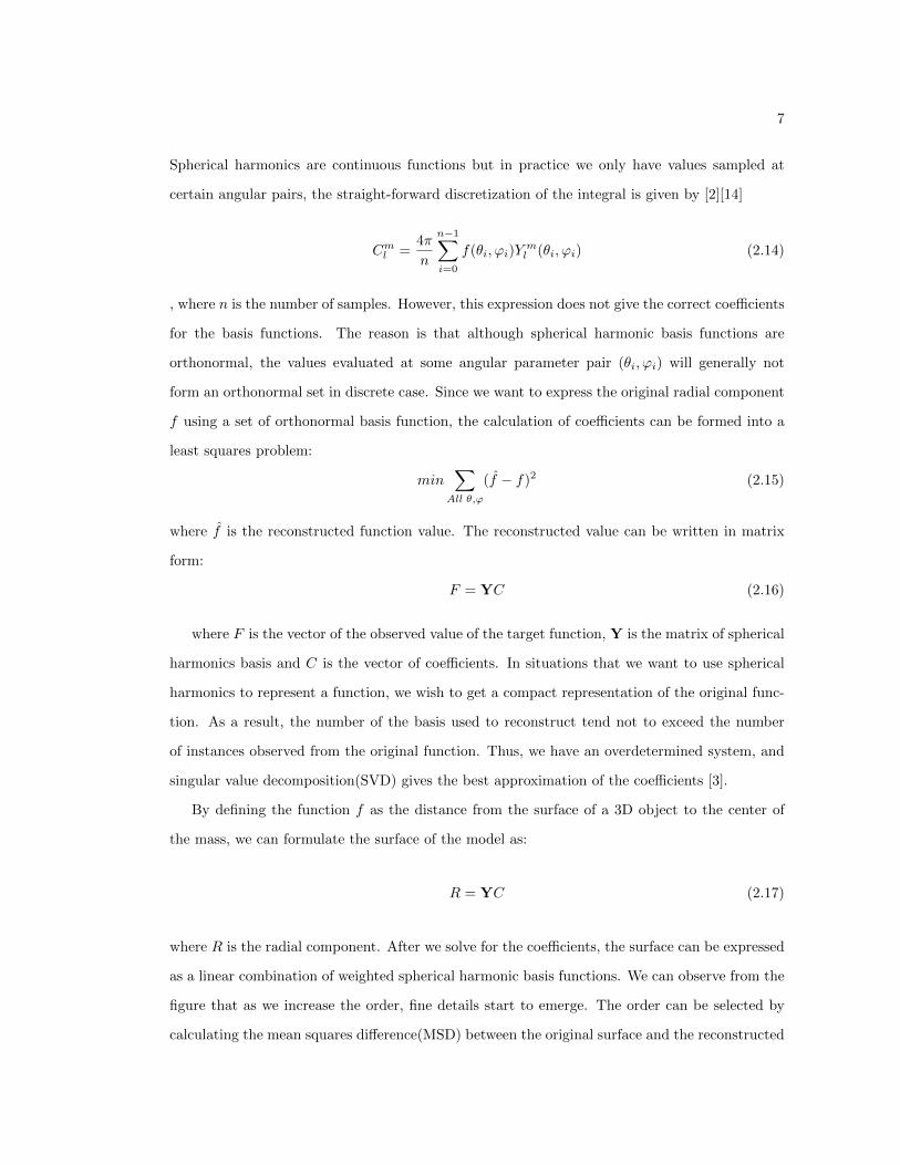
By defining the function f as the distance from the surface of a 3D object to the center of

the mass, we can formulate the surface of the model as:

R = YC (2.17)

where R is the radial component. After we solve for the coefficients, the surface can be expressed

as a linear combination of weighted spherical harmonic basis functions. We can observe from the

figure that as we increase the order, fine details start to emerge. The order can be selected by

calculating the mean squares difference(MSD) between the original surface and the reconstructed

8

Figure 2.2: Original surface(left), reconstructed surface with order 10(middle), reconstructedsurface with order20(right).

surface, and keep increasing the order until MSD is below some certain threshold. However, this

formulation is prone to rotation, and can only handle the model with a single radial component.

As such, spherical harmonics descriptor (SHD) is then used to decompose a 3D object into

a collection of spherical functions, where each function includes a series of spherical harmonic

functions [9][30]. In SHD, the 3D object is first rasterized into 2R ∗ 2R ∗ 2R voxel grid and the

center of mass is moved to (R,R,R). Second, the object is re-scaled so that the average distance

from the object voxels to (R,R,R) is R/2. Third, a set of concentric spheres are used to dissect

the 3D object and then determine the spherical harmonics representation on each sphere with

the radius r ∈ [0, R] and form the binary function fr which can be expressed using spherical

harmonics:

fr(θ, ϕ) =

L∑l=0

l∑m=−l

cml Yml (θ, ϕ) (2.18)

Finally, a rotation invariant descriptor is computed by taking the L2 norm of the sum within

each order l:

SH(fr) = {‖fr,0‖ , ‖fr,1‖ , ..., ‖fr,l‖ , ... ‖fr,L‖} (2.19)

where fr,l is the spherical harmonics component in the order l and

fr,l =

l∑m=−l

Cml Yml (θ, ϕ), l = 0, 1, ...L (2.20)

SHD is a generalization of the traditional spherical harmonic representation, which overcomes

the rotation invariant problem, and can be used on 3D objects that has more than one value in

the same colatitude and azimuth pair. However, SHD tends to have practical limitations.

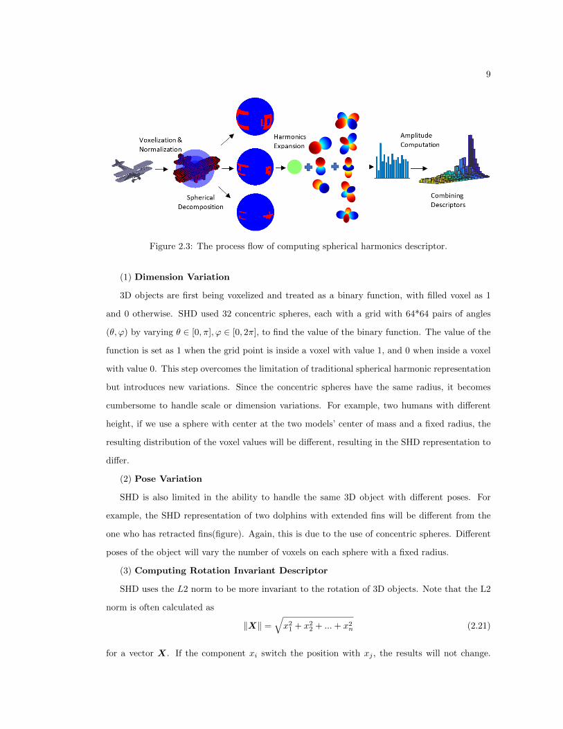
9

Figure 2.3: The process flow of computing spherical harmonics descriptor.

(1) Dimension Variation

3D objects are first being voxelized and treated as a binary function, with filled voxel as 1

and 0 otherwise. SHD used 32 concentric spheres, each with a grid with 64*64 pairs of angles

(θ, ϕ) by varying θ ∈ [0, π], ϕ ∈ [0, 2π], to find the value of the binary function. The value of the

function is set as 1 when the grid point is inside a voxel with value 1, and 0 when inside a voxel

with value 0. This step overcomes the limitation of traditional spherical harmonic representation

but introduces new variations. Since the concentric spheres have the same radius, it becomes

cumbersome to handle scale or dimension variations. For example, two humans with different

height, if we use a sphere with center at the two models’ center of mass and a fixed radius, the

resulting distribution of the voxel values will be different, resulting in the SHD representation to

differ.

(2) Pose Variation

SHD is also limited in the ability to handle the same 3D object with different poses. For

example, the SHD representation of two dolphins with extended fins will be different from the

one who has retracted fins(figure). Again, this is due to the use of concentric spheres. Different

poses of the object will vary the number of voxels on each sphere with a fixed radius.

(3) Computing Rotation Invariant Descriptor

SHD uses the L2 norm to be more invariant to the rotation of 3D objects. Note that the L2

norm is often calculated as

‖X‖ =√x21 + x22 + ...+ x2n (2.21)

for a vector X. If the component xi switch the position with xj , the results will not change.

10

Figure 2.4: Two dolphins with extended fins(left) and retracted fins(right). Each blue dot is anevaluated point of the discretized binary function

Figure 2.5: Different spherical functions give the same descriptor.

In other words, even if the harmonic coefficients Cml s are different or switched in positions, L2

norm can be the same although the distributions of voxels are different on concentric spheres.

Another problem caused by the L2 norm is the information loss. We know the norm of two

different vectors can be the same, thus, two different distribution of the binary values can have

the same L2 norm. Figure 2.5 illustrates this issue.

11

2.2 Empirical Representation

Empirical representation is developed using empirical practice. The light field descriptor (LFD)

[7] is proposed by deriving the geometric information and Fourier descriptor from 10 silhouettes

of a model in 10 uniformly distributed view angles, and in order to be robust to rotation, this

representation sometimes requires many LFDs to represent one single model. Furthermore, along

with the development of the convolutional neural network (CNN), 3D shape nets [22] and multi-

view CNN approach [23] are proposed to represent a 3D model using the convolution layer. The

idea behind these works is that if the object looks the same in all angles, it should be the same

object. However, these methods require a significant larger storage space for the representation

and computation cost than the math representations.

Aside from the viewing based representation, deep-learning is also very popular when com-

puting 3D model representations. DeepSDF[29] proposes to use the auto-encoder (AE) to find

the latent space of the signed distant function, which is a shape function that is zero when it is

on the surface, negative inside and positive outside the surface. They have successfully recreated

the surface information, yet their method needs the 3D object to be put in a canonical position.

Using the point cloud as input, [25] also uses AE to find the latent space and then regenerate the

structure using generative models. In their research, they have conducted experiments showing

the latent space features are rotation invariant under SVM classifier, yet they did not give proof

on it. MeshCNN[31] combines the convolution and pooling layer in the CNN by leveraging the

geodesic connections, i.e. the surface mesh. MeshCNN also allows the mesh to be less and more

refined. However, just as other machine learning algorithm, MeshCNN do require a decent set

of training data, and is sensitive to the variations in the training data.

What’s more, the representation that contains topological and structural information of a 3D

model is also considered feasible. The following methods avoid encountering the pose invariant

problem by focusing on capturing the topological information of the model. Model graph [8],

Reeb graph [6], and skeleton graph [10] representations are in general proposed. However, those

representations are limited to specific categories of 3D models. Other graph based representation

such as [21] first uses the voxel aggregation on the cloud point data of 3D objects, this step is

to filter out the noises. Then the sub-model is identified by the density of the voxel connection

and projected on a plane with minimum area, i.e. find the contour of the part, and is labeled

12

with the corresponding name. For example, if the contour is a circle, the sub-model will be

labeled ”cylinder”. After that, the labels are connected and a graph is created. However, this

approach is only suitable for 3D objects with ”linear” components such as pipes and cuboids.

Compared to deep-learning based approaches, the study of the preserving the inherent topological

and structural information of 3D models seem more plausible and computationally efficient. Kan

et al. explore the use of network representation for image profiles, which treats every pixel as

nodes and connect each pixel with other pixels with a weight computed using exponential kernel

[24]. Chen et al. investigated the use of recurrence network for analysis of spatial data [26] and

Yang et al. looked into the self-organizing topology of the network representation of complex

systems [20]. Few, if any previous work has been done to construct a self-organizing network

representation of 3D models.

2.3 Ideal Properties

These methods are more concerned about 3D shapes and focus less on the internal structure of

3D objects. Hence, there is an urgent need to develop an effective representation of 3D objects

that provides the following advantageous features:

1) Rotation Invariant: In the absence of prior knowledge, 3D objects found online can be

rotated and placed in different ways. Thus, the representation should be consistent despite its

scale, orientation, and position.

2) Shape and Internal Structure: There are many engineering designs that are similar in

the shape but differ in the internal structures. An effective representation should capture the

inherent characteristics of the geometric and topological structure of 3D objects.

3) Compactness: When presenting the information of 3D objects in alternative domains, the

representation should be compact enough so that mathematical description of salient patterns

and the procedures for feature extraction are more efficient and much simpler.

4) Multi-resolution Representation: There are large-scale (i.e., approximations) and small-

scale (i.e., details) information for a 3D object. An effective representation should provide both

the big picture and fine-grained details of 3D objects to serve the purpose of the users.

Chapter 3Self-organizing Network Modelling

In this chapter, we discuss our proposed method. The method is two-fold: network representation

and self-organizing modelling. The network representation builds a 3D object representation

in the matrix form and the self-organizing modelling helps to validate the effectiveness of the

representation by finding the minimum-energy layout of the network nodes.

3.1 A Brief Introduction of Network Representation

The origin of using network to formulate a real-life problem is the Konigsberg puzzle, or ”The

Seven Bridges of Konigsberg”. This historically notable problem in mathematics requires people

to find a way to cross the seven bridges that divide the land of Konigsberg into four pieces

once and only once. Leonhard Euler first points out the route inside the four landmasses are

irrelevant to the problem and the only important feature is the sequence of the bridges crossed.

This allows Euler to formulate the problem using a network representation—the four land masses

are abstracted as four vertices, and the seven bridges are formulated as seven edges that connect

the four vertices. After that Euler gave a proof that there is no such route to travel between

the four landmasses and go across each bridge only once. Euler’s solution laid the foundation of

graph theory and the idea of network topology.

14

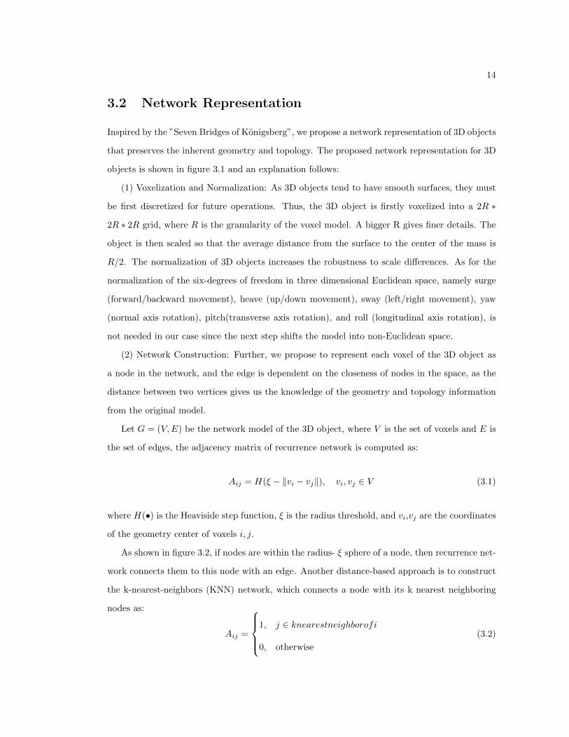
3.2 Network Representation

Inspired by the ”Seven Bridges of Konigsberg”, we propose a network representation of 3D objects

that preserves the inherent geometry and topology. The proposed network representation for 3D

objects is shown in figure 3.1 and an explanation follows:

(1) Voxelization and Normalization: As 3D objects tend to have smooth surfaces, they must

be first discretized for future operations. Thus, the 3D object is firstly voxelized into a 2R ∗

2R ∗ 2R grid, where R is the granularity of the voxel model. A bigger R gives finer details. The

object is then scaled so that the average distance from the surface to the center of the mass is

R/2. The normalization of 3D objects increases the robustness to scale differences. As for the

normalization of the six-degrees of freedom in three dimensional Euclidean space, namely surge

(forward/backward movement), heave (up/down movement), sway (left/right movement), yaw

(normal axis rotation), pitch(transverse axis rotation), and roll (longitudinal axis rotation), is

not needed in our case since the next step shifts the model into non-Euclidean space.

(2) Network Construction: Further, we propose to represent each voxel of the 3D object as

a node in the network, and the edge is dependent on the closeness of nodes in the space, as the

distance between two vertices gives us the knowledge of the geometry and topology information

from the original model.

Let G = (V,E) be the network model of the 3D object, where V is the set of voxels and E is

the set of edges, the adjacency matrix of recurrence network is computed as:

Aij = H(ξ − ‖vi − vj‖), vi, vj ∈ V (3.1)

where H(•) is the Heaviside step function, ξ is the radius threshold, and vi,vj are the coordinates

of the geometry center of voxels i, j.

As shown in figure 3.2, if nodes are within the radius- ξ sphere of a node, then recurrence net-

work connects them to this node with an edge. Another distance-based approach is to construct

the k-nearest-neighbors (KNN) network, which connects a node with its k nearest neighboring

nodes as:

Aij =

1, j ∈ knearestneighborofi

0, otherwise

(3.2)

15

Figure 3.1: The flowchart of network representation of 3D objects.

Note here in both approaches, the diagonal element is subtracted. Figure 3.3 shows the

sparsity pattern of the adjacency matrix for the recurrence network and KNN network of the

chair. We can see the general shape are almost identical, while the KNN network can be non-

symmetric. We will further discuss and compare the performance of both recurrence network

and KNN approaches for the representation of 3D objects in Section 4.

With both network generation approaches, the original 3D model can now be converted into

adjacency matrices. Here the adjacency matrices are sparse, thus can be further compressed in

the form of sparse matrices, which essentially is the edge list of the network. This makes our

network representation concise to storage.

3.3 Self-organizing Network Modelling

The adjacency matrix contains the connectivity information among nodes of a network model,

but the network topology can change while preserving the node-to-node connectivity in the

adjacency matrix. In figure 3.3, the two networks have the same connectivity, but their layouts

are different, this poses a question that how do we determine, or tell which network layout is

”correct”, or ”better”. In figure 3.1, one can never tell the network representation on the right

is a chair.

Therefore, we propose to derive the self-organizing network model to find the stable topology

when the network energy is minimized to reach the steady period. Our prior studies have de-

veloped network models of 2D image profiles for manufacturing quality control [24], and further

leveraged recurrence networks to predict the quality of surface finishes in the ultra-precision ma-

chining [26]. In addition, we studied the self-organizing topological structures for network models

of classical nonlinear systems (i.e., Lorenz and Rossler systems) [20] and variable clustering using

16

Figure 3.2: The illustrations of recurrence network vs. K-nearest-neighbors network methods.

self-organizing network.[]

However, very little has been done to study the self-organizing network models of 3D objects.

Our prior studies laid the groundwork and motivated the present study to develop an effective

representation of 3D objects (e.g., engineering designs, 3D scans, point clouds) with network

models.

In this investigation, we first derive the adjacency matrix with the network construction

method (e.g., recurrence network or KNN approaches) and then utilize the spring-electrical model

to drive the network to self-organize into an optimal layout. The model has two forces, namely

the attractive force and repulsive force [1][13][20]. The repulsive force exists between any two

pair of nodes in the model, and is inversely proportional to the distance between them. The

repulsive force RF can be computed as:

RF (i, j) = − CKp+1

‖vi − vj‖p(vi − vj), vi 6= vj , p > 0 (3.3)

17

Figure 3.3: Sparsity pattern of Adjacency Matrix(middle) with threshold ξ of 2√

2 and TransitionMatrix(right) with k equal to 20.

Figure 3.4: A graph have same adjacency matrix can have various layouts(Graph Isomorphism).

The attractive force, on the other hand, only exists between two connected pair of nodes, and is

proportional to the squared distance between the two nodes. The attractive force is computed

as:

AF (i, j) =‖vi − vj‖

K(vi − vj), vi ↔ vj (3.4)

where vi ↔ vj denotes node i and node j are connected, (vi − vj) is the force-directional vector,

K is the natural spring length, and C is the parameter regulates the relative strength of the

repulsive and attractive force. The objective is to find the optimal layout by minimizing the

total energy of the system.

18

Figure 3.5: Peripheral effect of spring-electrical model, only the nodes are shown. We can observethe nodes in the peripheral area tend to cluster.

Energy(V,K,C) =∑i∈V

f2(i, vi,K,C) (3.5)

f(i, vi,K,C) =∑vi 6=vj

− CKp+1

‖vi − vj‖(vi − vj) +

∑vi↔vj

‖vi − vj‖K

(vi − vj) (3.6)

where f(i, vi,K,C) is the combined force on the node i. The network energy can be minimized

iteratively by moving the vertices in the direction of the total force exerted on them. Intuitively,

in the spring-electrical model, we can think that network nodes are simulated as electrically

charged particles, and the edges are simulated as springs, each node propels other nodes and are

bonded by connected edges. The minimum energy is achieved only when all the forces between

the nodes reaches equilibrium.

The layout of the self-organizing network can be computed using an iterative scheme [1][12],

Algorithm 1 demonstrates the workings:

Since the objective is to find the minimum energy layout, we use a stopping criteria which

stops the algorithm when the energy is decreasing in the current iteration, the energy is increasing

in the previous iteration, and the ratio between the difference between the energy in two iterations

and the current energy is below a threshold, we say the network has reached a minimum energy

layout.

For the step length in the algorithm, just as the learning rate in gradient descent algorithm,

is necessary to be updated. A larger step length can reach the final state faster while a smaller

step is more reliable for reaching convergence. In here, we keep increase the step length for five

iterations, and we set it back to the original value. This step length updating algorithm is shown

in Algorithm 2.

19

Algorithm 1 Force-directed Algorithm for finding the minimum energy layout iteratively

FUNCTION ForceDirectedAlgorithm (G,x,tolerance)

INPUT:Graph G, initial random layout x, tolerance for the energy convergence

OUTPUT: Minimum energy layout x

1: converged = FALSE2: step = initialsteplength3: Energy = Inf4: EnergyArray = []5: while converged == FALSE do6: x0 = x7: Energy0 = Energy8: EnergyArray.append(Energy0)9: Energy = 0

10: for i ∈ G.vertices do11: f = 012: for j ∈ G.vertices and i, j connected do13: f = f +AF (i, j)

14: for j ∈ G.vertices and i 6= j do15: f = f +RF (i, j)

16: xi = xi + step ∗ (f/||f ||)17: Energy = Energy + ||f ||2

18: step = updateStepLength(step, Energy,Energy0)19: if EnergyArray(end) > EnergyArray(end − 1) and EnergyArray(end − 1) >

EnergyArray(end− 2) and |Energy−EnergyArray(end−2)|Energy < tolerance then20: converged = TRUE

21: return x

Algorithm 2 Adaptive step length for better convergence

FUNCTION updateStepLength(step,Energy,Energy0)

INPUT:step,Energy,Energy0

OUTPUT: updated step

1: progress = 02: t = 0.983: if Energy < Energy0 then4: progress = progress+ 15: if progress >= 5 then6: progress = 07: step = step/t

8: else9: progress = 0

10: step = t ∗ step11: return step

20

The parameter in the spring electrical model can also have an effect on the layout. If we

increase the value of parameter K, this will result in a higher amplitude of repulsive force and a

smaller attractive force, thus the space between each node will be larger. Parameter C regulates

the relative intensity of the attractive and the repulsive forces between two vertices. Parameter

C only exists in the repulsive force, and a higher value of C will increase the repulsive force. It

was shown that changing K and C will not alter the final network topology with the minimal

energy, but just re-scale the layout in ref. Based on prior empirical results, we choose K to be 1

and C to be 0.2 in this present study. Parameter p is used to weaken the peripheral effect, which

is shown in figure 3.5, and will be discussed in chapter 4.

Chapter 4Experimental Design and Results

In this chapter, we evaluate and validate the performance of self-organizing network representa-

tion of 3D objects with respect to three factor groups, namely network construction method, the

model parameter p, and voxelization granularity:

1)In Chapter 3, we mentioned two distance-based network construction methods namely the

recurrence network and KNN network. These two networks both connect each node with its

neighbors, in recurrence network, the neighbors within a fixed radius are connected, while in

KNN network, we only connect a fixed number of nearest neighbors.

The first question is “which network construction method is better? Recurrence network or

KNN network?” This is perhaps the key factor since the following steps and the analysis of the

final layout of the self-organizing network is based on the adjacency matrix generated in this

step.

2)An intrinsic characteristic of the spring-electrical model is that the vertices in the periphery

have a trend to cluster closer than the ones in the middle. The peripheral effect is illustrated in

figure 3.5, in which we can see the leg of the chair tend to be dense. Parameter p helps reduce

the peripheral effect in the self-organizing process. A bigger p will reduce long-range repulsive

force, and then cause the peripheral nodes to disperse.

Thus, the second question is to find out which p value is better in this self-organizing network

representation of 3D objects?

3)The granularity in the voxelization step is critical to examine the approximations and details

of 3D objects. Typically, a finely detailed model is desired, while in our case, since our network

22

Figure 4.1: Cause and effect diagram for evaluation of self-organizing network representation

representation allows multi-resolution representation, the level of details can be chosen when

considering the approximation-detail trade-off. Ideally, a detailed model is desired, however, an

approximation can be more robust under noises and variations. We will investigate whether and

how voxelization granularity impacts the performance of self-organizing network.

As a result, the third question is to find the impact of the granularity on the performance of

the self-organizing network.

The fish-bone diagram of the experimental design is shown in figure 4.1 for visualizing our

design. In the experiments, the adjacency matrix is first computed using distance-based network

construction methods with the input of the granularity of the representation. Then the vertices

in the network are randomly initialized in 3D space with only the input of the adjacency matrix

from the last step and the model parameter p. Then we run the self-organizing algorithm to find

and record the layout of the network along with its system energy.

4.1 Recurrence Network vs. KNN network

As shown in figure 3.3, we identified two distance-based network construction methods, the

recurrence network and KNN network. In recurrence network, the radius threshold ξ needs to be

pre-specified, and in KNN network the number of nearest neighbors, k, needs to be chosen. As

shown in figure 4.2, if we choose the threshold too small, there’s not enough connectivity in the

network, and a very large threshold will create some unwanted clusters, i.e. the legs of the chair

may be considered to be together. As a result, we want to choose a moderate threshold for the

23

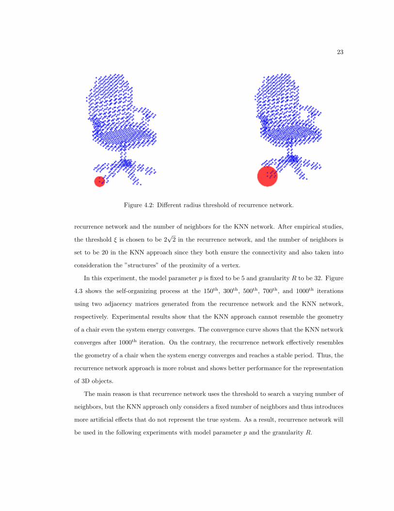
Figure 4.2: Different radius threshold of recurrence network.

recurrence network and the number of neighbors for the KNN network. After empirical studies,

the threshold ξ is chosen to be 2√

2 in the recurrence network, and the number of neighbors is

set to be 20 in the KNN approach since they both ensure the connectivity and also taken into

consideration the ”structures” of the proximity of a vertex.

In this experiment, the model parameter p is fixed to be 5 and granularity R to be 32. Figure

4.3 shows the self-organizing process at the 150th, 300th, 500th, 700th, and 1000th iterations

using two adjacency matrices generated from the recurrence network and the KNN network,

respectively. Experimental results show that the KNN approach cannot resemble the geometry

of a chair even the system energy converges. The convergence curve shows that the KNN network

converges after 1000th iteration. On the contrary, the recurrence network effectively resembles

the geometry of a chair when the system energy converges and reaches a stable period. Thus, the

recurrence network approach is more robust and shows better performance for the representation

of 3D objects.

The main reason is that recurrence network uses the threshold to search a varying number of

neighbors, but the KNN approach only considers a fixed number of neighbors and thus introduces

more artificial effects that do not represent the true system. As a result, recurrence network will

be used in the following experiments with model parameter p and the granularity R.

24

Figure 4.3: The self-organizing process of KNN vs. recurrence network for a chair and theirconvergence curves (parameter p=5, granularity 32). For the purpose of better visualization,edges are not plotted in the figure.

4.2 Effects of model parameter p

At the end of chapter 3 we introduced the peripheral effect of the spring-electrical model. The

vertices in the periphery tend to cluster and the layout with converged energy may not be

satisfactory. To alleviate this problem, the model parameter p can be used to give a satisfactory

result.

25

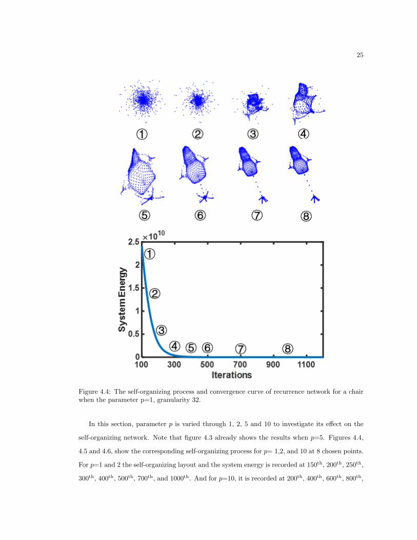
Figure 4.4: The self-organizing process and convergence curve of recurrence network for a chairwhen the parameter p=1, granularity 32.

In this section, parameter p is varied through 1, 2, 5 and 10 to investigate its effect on the

self-organizing network. Note that figure 4.3 already shows the results when p=5. Figures 4.4,

4.5 and 4.6, show the corresponding self-organizing process for p= 1,2, and 10 at 8 chosen points.

For p=1 and 2 the self-organizing layout and the system energy is recorded at 150th, 200th, 250th,

300th, 400th, 500th, 700th, and 1000th. And for p=10, it is recorded at 200th, 400th, 600th, 800th,

26

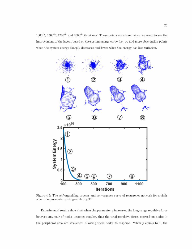
1000th, 1500th, 1700th and 2000th iterations. These points are chosen since we want to see the

improvement of the layout based on the system energy curve, i.e. we add more observation points

when the system energy sharply decreases and fewer when the energy has less variation.

Figure 4.5: The self-organizing process and convergence curve of recurrence network for a chairwhen the parameter p=2, granularity 32.

Experimental results show that when the parameter p increases, the long-range repulsive force

between any pair of nodes becomes smaller, thus the total repulsive forces exerted on nodes in

the peripheral area are weakened, allowing these nodes to disperse. When p equals to 1, the

27

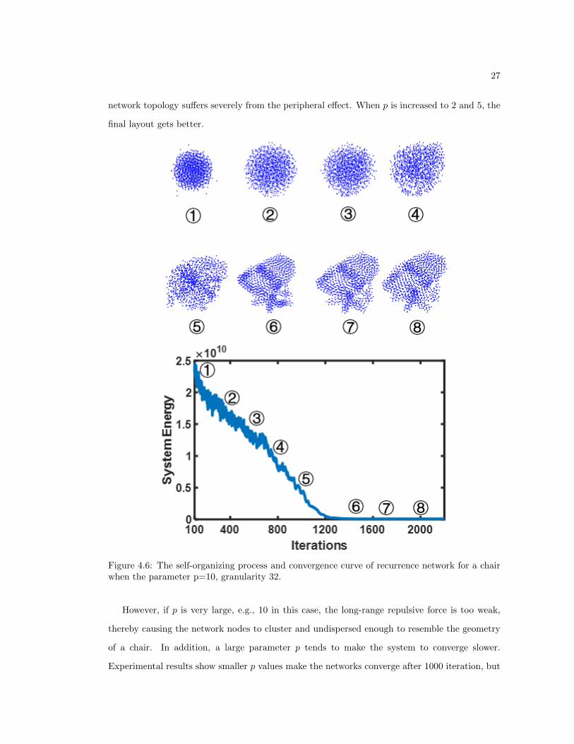
network topology suffers severely from the peripheral effect. When p is increased to 2 and 5, the

final layout gets better.

Figure 4.6: The self-organizing process and convergence curve of recurrence network for a chairwhen the parameter p=10, granularity 32.

However, if p is very large, e.g., 10 in this case, the long-range repulsive force is too weak,

thereby causing the network nodes to cluster and undispersed enough to resemble the geometry

of a chair. In addition, a large parameter p tends to make the system to converge slower.

Experimental results show smaller p values make the networks converge after 1000 iteration, but

28

a larger p (e.g.,10) takes more iterations (>1500) to converge. Hence, this present study chose

p = 5.

4.3 Effects of voxelization granularity

Figure 4.7: The self-organizing process of recurrence network for a chair when the parameterp=5, granularity 64.

29

Further, we investigate whether and how voxelization granularity (i.e., R=32 and 64) impacts

the performance of self-organizing network. Note that figure 4.3 to 4.6 already show the results

when R=32. Here, we focus on the granularity R=64 for three different objects (i.e., chair, ant,

and airplane). The self-organized layout is shown at 100th, 150th, 250th, 500th, 1000th, 1500th,

2000th, and 2500th. Experimental result is shown in figure 4.7, in which we can observe when

the granularity increases, network representation captures finer details of the 3D object and the

geometry and structure become clearer.

However, the higher the granularity is, there will be more voxels in the network model. This,

in turn, increases the computational complexity in the self-organizing process. For example,

the network with granularity 64 yields a slower convergence than granularity 32. In practice,

the level of granularity depends to a great extent on the objective of users to balance between

computational efficiency and model granularity. Our future work will further investigate the

multi-resolution network representation that accounts for both the approximations and details

to increase robustness to uncertainty.

In figure 4.8 we have shows the results for other models. On the left is the original 3D object

and on the right is the layout of self-organizing network with converged energy. We can see that

in both models the self-organizing network show that the adjacency matrix can be successfully

reconstructed into a structure that preserves the geometry and structure of the original model.

Figure 4.8: The self-organizing process of recurrence network for an ant, and a plane when theparameter p=5, granularity 64.

Chapter 5Network Representation Matching

In this chapter, we extract features from the network representations and use variable selection

to reduce the number of features, then we train classifiers to classify the representations and

compare with spherical harmonic descriptor(SHD)[11].

5.1 Research Background

Network similarity is a very broad topic when it comes to concurrent researches, different ap-

proaches are being proposed in recent years. Researchers are dedicated to find a measure of

similarity between two networks, to perform network alignment and classification. There are two

major categories of the similarity measure—Matrix multiplication based and feature based.

IsoRank[14][18] algorithm is a classic matrix multiplication based method and is proposed

to find the node alignment of two networks, even with different sizes. The IsoRank algorithm

computes the node-to-node similarity score by considering the two networks as a new network,

with nodes as the node pairs from two networks, and connects the two nodes when they are all

connected in the previous networks. After that, it uses a random walk to find the time one stays

in each node and iteratively calculates the fraction it stays in these nodes. Then the nodes are

being aligned using a greedy algorithm, matching two nodes with the highest similarity score, and

proceeds. The overall similarity is computed using maximum shared edges in the aligned graph

divided by the min(number of edges in GA, number of edges in GB). Other matrix multiplication

based methods such as [16] uses the in/out degree of a node to compute network similarity score.

31

However, through our experiments, we observe that these network algorithms tend to align two

nodes with the same degree and does not work well in our case.

NetSimile[19] is a feature based approach to calculate the similarity. NetSimile is based on

using the features extracted from the network, namely the network measures, to compute the

similarity. Feature based network similarity also uses density of eigenvalue of the network[17],

entropy, fielder vector, and energy[28]. These kinds of network similarity measures are intuitive

and have decent accuracy.

As a result, in this work, we first identify the features and extract them, and we use a pruning

method to conduct feature selection, reducing the number of features in our model and test its

performance.

5.2 Network Identity and Features

Networks are expressed as G = (V,E), where V is the set of vertices, and E is the set of edges

that connect two nodes. Another representation is the matrix representation, where G can be

expressed as an adjacency matrix that contains the connectivity information between two nodes.

Thus, the identity and the feature of a network can be given both as network statistics and

matrix-based features.

The network statistics give meaningful information to the identity of a network, for example,

node degree, link density, network diameter, centrality, and average path length, all express some

of the important characteristics of a network.

As for the characteristics of the adjacency matrices, for example, the eigenvalues for the

adjacency matrix, the eigenvalues for the laplacian matrix, the determinant of the matrix, and

etc.

There’s no telling one feature is superior to another. As a result, we propose to first extract

as many features from the network as possible and then use a variable selection scheme to extract

useful features for our network representation, and then use these features to match two networks.

The features can be categorized into global measures and local measures. Global measure is

the overall measure of the network, for example, the diameter of the network. Local measure

is the measure on the vertices and edges of the network, for example, clustering coefficient and

the degree distribution of the nodes. For local measures, in order to tackle the variation of the

32

number of vertices for different network representations, we measure the for moments of the local

features—mean, standard deviation, skewness, and kurtosis. The four moments are calculated

as follows:

µ =1

n

n∑i=1

xi (5.1)

σ =

√∑ni=1(xi − µ)2

n(5.2)

s =1n

∑ni=1(xi − µ)3

1n−1

∑ni=1(xi − µ)

3/2(5.3)

k =1n

∑ni=1(xi − µ)4

( 1n−1

∑ni=1(xi − µ)

2)2

(5.4)

where xi is the value of the local measures. If we perceive the local measures as a distribution,

mean gives us the average of the local measures, the standard deviation tells how disperse the

measures are, the skewness gives the information of how the shape of the distribution is shifted

relative to the mean and kurtosis tells how outlier-prone a distribution is.

5.3 Feature Extraction

We first extract the network features, we start with the degree distribution. The degree of a node

can be calculated as the number of neighboring nodes ki =∑nj=1Aij , where n is the number

of vertices in the network, and A is the adjacency matrix. Next, we compute the shortest path.

The shortest path is defined as the shortest distance between two nodes, and the maximum value

of the shortest path is called the network diameter. After that, we compute the centrality.

Centrality is a measure of node importance in a network, and can have different measures.

We use the closeness centrality, which is the inverse sum of the shortest paths from a node to all

other nodes in the graph. The betweenness centrality is also collected since it measures how often

each vertex appears on the shortest path between two other vertices in the network. Pagerank

centrality is also useful, since it is the result of a random walk on the network. After that,

we calculate the global efficiency of the network, which measures the efficiency of the vertices

exchanging information with each other.

Clustering coefficient can also be a local measure to determine the importance of nodes. The

clustering coefficient is defined as 3 times the number of triangles in the network divided by the

33

number of connected triples of vertices, where a triple is a vertex whose edge runs into another

pair of connected nodes.

Finally, we calculate the graph density, which is defined as the ratio between all edges of

the network and the maximum number of edges. This can be helpful when distinguishing two

networks in which one of them is densely connected, for example, a tank, and the other one is

not so dense, for example, a tree.

Secondly, we extract features from the adjacency matrix. One important feature of the matrix

is its eigenvalues and eigenvectors. The definition of eigenvalue and eigenvector is given by

Au = λu (5.5)

where A is the matrix, u is the eigenvector, and λ is the eigenvalue corresponding to the eigen-

vector. Intuitively, a matrix conducts a linear transformation of a vector, and the eigenvector is

the direction of the transformation that by applying the linear transformation A, the direction

remains unchanged. As a result, we think this can be an important feature. The eigenvalues of

an adjacency matrix is also called the spectrum of the matrix, and since the adjacency matrix is

symmetric, the singular value decomposition of an adjacency matrix can be in the form of

A = UΣUT (5.6)

where the Σ matrix is a diagonal matrix whose entries are a descending series of eigenvalues.

As a generalization of the adjacency matrix, another useful representation of the network is

the laplacian matrix. The laplacian matrix is defined as

L = D −A (5.7)

where D is a diagonal matrix with the degree of the node as its entry. One important application

using the laplacian matrix is graph clustering. The eigenvector corresponding to the minimum

non-zero eigenvalue of the laplacian matrix is called the Fielder vector, and is used for finding

the minimum cut of a graph. Thus, we include the largest 20 and smallest 20 eigenvalues of

the adjacency matrix and laplacian matrix to achieve consistency when the number of nodes is

different. In addition, we also included the matrix power and matrix index in our matrix features

34

Table 5.1: Extracted features

Degree Four MomentsDiameterShortest Path Four MomentsGlobal EfficiencyBetweenness Centrality Four MomentsPageRank Centrality Four MomentsEigenvector Centrality Four MomentsCloseness Centrality Four MomentsClustering CoefficientDensityPagerank Largest and Smallest 20Eigenvalue Adjacency Matrix Largest and Smallest 20Index of MatrixEigenvalue Laplacian Matrix Largest and Smallest 20Matrix Power Power of 2 and 3

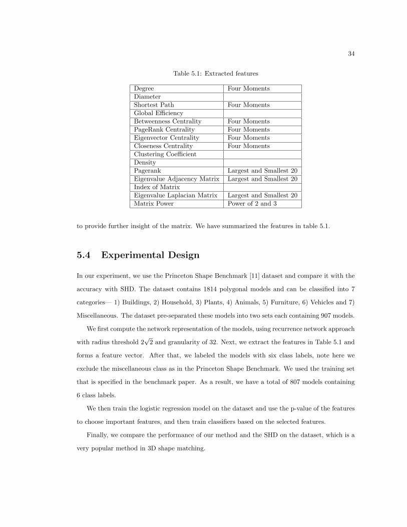
to provide further insight of the matrix. We have summarized the features in table 5.1.

5.4 Experimental Design

In our experiment, we use the Princeton Shape Benchmark [11] dataset and compare it with the

accuracy with SHD. The dataset contains 1814 polygonal models and can be classified into 7

categories— 1) Buildings, 2) Household, 3) Plants, 4) Animals, 5) Furniture, 6) Vehicles and 7)

Miscellaneous. The dataset pre-separated these models into two sets each containing 907 models.

We first compute the network representation of the models, using recurrence network approach

with radius threshold 2√

2 and granularity of 32. Next, we extract the features in Table 5.1 and

forms a feature vector. After that, we labeled the models with six class labels, note here we

exclude the miscellaneous class as in the Princeton Shape Benchmark. We used the training set

that is specified in the benchmark paper. As a result, we have a total of 807 models containing

6 class labels.

We then train the logistic regression model on the dataset and use the p-value of the features

to choose important features, and then train classifiers based on the selected features.

Finally, we compare the performance of our method and the SHD on the dataset, which is a

very popular method in 3D shape matching.

35

5.5 Experimental Results

We first conducted a ”big bang” test, using all the features to train multiple classification models,

the models are selected based on 10-fold cross-alidation error. We found the support vector

machine classifier with a quadratic kernel has the most accuracy of 74.5%. The confusion matrix

is given in figure 5.1 to examine the type I and type II errors. The green column on the right is

the true positive rate, and the red column is the false positive rate. True positive rate is defined

as:

TPR =TruePositive

TruePositive+ FalseNegative(5.8)

and false negative rate is defined as

FNR =FalsePositive

TruePositive+ FalseNegative(5.9)

Figure 5.1: Confusion matrix for Quadratic SVM with all features.

36

We can see from the confusion matrix, the accuracy for the household and vehicle class is

high, with moderate accuracy for the animal and furniture class, with not so satisfying accuracy

on the plant and building class.

Figure 5.2: p-value of 148 features for 5 logistic regression models.The features are sorted byascending p-value

However, currently we have a feature vector of 148 columns, and only 807 instances, we

wonder if the accuracy will remain the same or increase when we reduce the number of features.

Not to mention reducing the number of features can increase feature extraction time.

First, we try to use the principal component analysis(PCA) to reduce the dimensionality of the

data. PCA conducts a linear transformation on the data and picks the linear combinations of the

data based on the variance explained. In our case, we tried the 95% and 99% variance explained

and we found the overall accuracy to be 62.9% and 69.1% with 9 features and 20 features,

respectively. However, PCA has low interpretability, and we cannot know which features are

important, not to mention the accuracy has dropped about 7 percent.

37

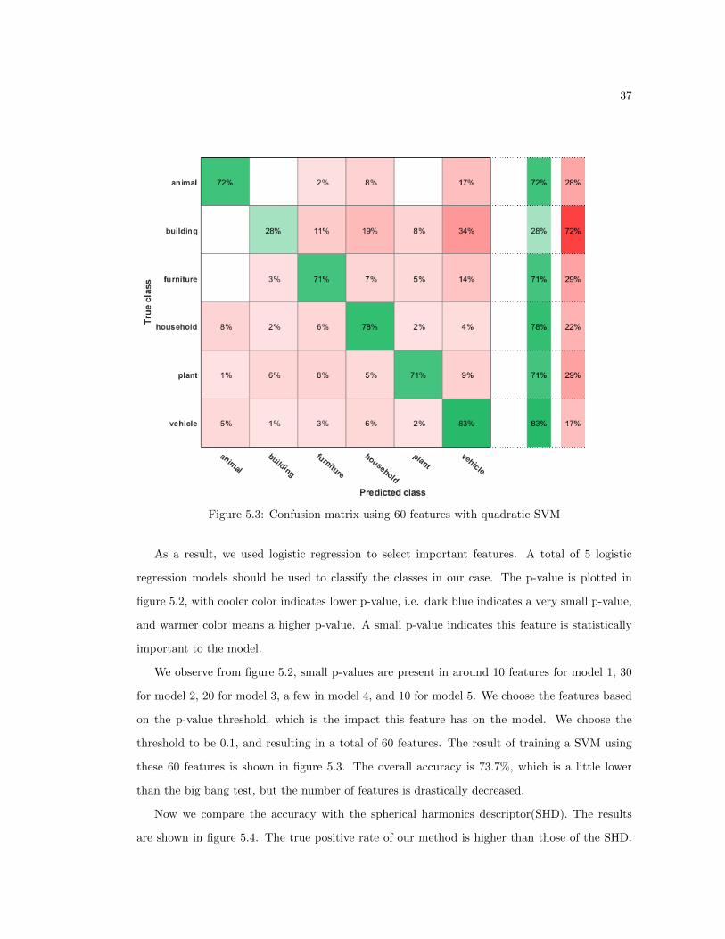
Figure 5.3: Confusion matrix using 60 features with quadratic SVM

As a result, we used logistic regression to select important features. A total of 5 logistic

regression models should be used to classify the classes in our case. The p-value is plotted in

figure 5.2, with cooler color indicates lower p-value, i.e. dark blue indicates a very small p-value,

and warmer color means a higher p-value. A small p-value indicates this feature is statistically

important to the model.

We observe from figure 5.2, small p-values are present in around 10 features for model 1, 30

for model 2, 20 for model 3, a few in model 4, and 10 for model 5. We choose the features based

on the p-value threshold, which is the impact this feature has on the model. We choose the

threshold to be 0.1, and resulting in a total of 60 features. The result of training a SVM using

these 60 features is shown in figure 5.3. The overall accuracy is 73.7%, which is a little lower

than the big bang test, but the number of features is drastically decreased.

Now we compare the accuracy with the spherical harmonics descriptor(SHD). The results

are shown in figure 5.4. The true positive rate of our method is higher than those of the SHD.

38

Figure 5.4: Confusion matrix for SHD

However, we can observe that the SHD also does poorly on the building class, so we consider

this might be a confounding class so we removed it.

By removing the building class, we use our selected network features on the dataset, the

number of objects is now 754. The results are shown in figure 5.5, and the overall true positive

rate is pretty high. Notably we also train the SHD features on the selection of classifiers and

interestingly, we find the quadratic SVM gives the best result. The TPR is recorded for both

methods.

Here, we give an overall comparison between the classification results of our network features

and SHD in Table 5.2. The overall TPR for every class is higher than that of SHD even using

the classifier that has the highest accuracy.

As a result, we conclude our method has better accuracy in classifying the objects in the

dataset. Next, we want to examine the results and try to interpret them.

We first look at the selected features. We conclude the following features can summarize the

39

Table 5.2: Comparison of Results

Comparison on Classification Results(TPR)Network Representation SHD

Animal 77% 67%Furniture 69% 62%Household 80% 70%Plant 71% 65%Vehicle 85% 83%

”identity” of our network representation for 3D objects: Degree distribution, shortest path, global

efficiency, betweenness centrality, closeness centrality, eigenvector centrality, clustering coefficient,

determinate of adjacency matrix, and eigenvalues for the adjacency matrix and laplacian matrix.

Next, we examine the confusion matrix for our method. In figure 5.3 we can see that the

animal, furniture, household, and plant class all have the highest false negative rate compared

to vehicle. This is probably caused by some of the vehicles having similar topological structures

like models in other classes.

Chapter 6Conclusions and Future Work

6.1 Conclusions

This thesis presents a self-organizing network representation of 3D objects that enables and

assists in the matching and retrieval of engineering designs in a searchable database. As such,

manufacturing engineers will not need to “reinvent the wheel”, but search and retrieve digital

designs and optimal process plans that are accumulated in the past practice. This will save a

tremendous amount of time, effort and investment, thereby advancing the paradigm of smart

manufacturing for personalized designs and mass customization.

In the present study, we first voxelize and normalize a 3D model. Then, a distance-based

network construction is introduced, recurrence network and k-nearest neighbor network, to gen-

erate a network (matrix) representation of the model. However, given network isomorphism, i.e.

a network can have different layouts when preserving the connectivity, we cannot simply tell if

the network representation is good or bad. We propose to use the force-directed graph drawing—

spring electrical model to simulate the nodes in the network to be charged particles that propels

all other nodes and edges to be springs that pull two nodes together. By minimizing the total

energy contained in this system, a stable layout can be reached. There are a few variations that

can affect the layout of the spring-electrical model, namely the network construction method,

model parameter, and granularity. We conducted experiments to tune the model such that the

result is acceptable.

Experimental results show that self-organizing network tackles persistent challenges by tra-

41

ditional representation methods as of the state of the art, and effectively captures inherent topo-

logical and geometric characteristics of 3D objects. When the system energy is minimized and

reaches a stable period, recurrence network effectively resembles the geometry of a 3D object.

Next, We also showed an intuitive way to match two network representations generated by

recurrence network using the Princeton Shape Benchmark dataset. We identified a handful of

network features and we use them to train classifiers. A big bang test is launched and we found

the SVM with quadratic kernel gives the best result. Since the current number of features is

nearly 150, we use a variable selection method to prune the features. Logistic regression is used

since it has the least assumptions and very easy to train. We used the p-values associated with

each feature in the 5 logistic regression models, note logistic regression is a binary classifier and

we need n−1 models to classify n classes. We then use the selected features to train the SVM and

we found the TPR is better than that of SHD. Since originally the SHD uses KNN classification,

we used SVM to boost its accuracy, and our method still outperforms SHD.

6.2 Future Work

Though our intuitive network matching works well, we need to investigate better ways of network

matching. As a result, we will be working on finding an algorithm to match two networks, or

even part of the networks (sub-graph matching), with a higher accuracy.

In addition, an efficient indexing framework should be developed to make the matching and

retrieval of 3D models faster, and by combining all these together, a searchable database of 3D

objects can be realized.

Bibliography

[1] T. M. J. Fruchterman and E. M. Reingold, “Graph Drawing by Force-directed Placement,”Softw., Pr. Exper., vol. 21, pp. 1129–1164, 1991.

[2] C. H. Brechbuhler, G. Gerig, and O. Kubler, “Parametrization of closed surfaces for 3-Dshape description,” Comput. Vis. Image Underst., 1995.

[3] S. Erturk and T. J. Dennis, ”3D model representation using spherical harmonics,” in Elec-tronics Letters, vol. 33, no. 11, pp. 951-952, 22 May 1997

[4] M. Ankerst, G. Kastenmuller, H.-P. Kriegel, and T. Seidl, “3D Shape Histograms for Simi-larity Search and Classification in Spatial Databases,” in Proceedings of the 6th InternationalSymposium on Advances in Spatial Databases, pp. 207–226, 1999.

[5] D. V. Vranic, D. Saupe, and J. Richter, “Tools for 3D-object retrieval: Karhunen-Loevetransform and spherical harmonics,” in 2001 IEEE Fourth Workshop on Multimedia SignalProcessing, pp. 293–298, 2001.

[6] S. Biasotti, S. Marini, M. Mortara, G. Patane, M. Spagnuolo, and B. Falcidieno, “3D ShapeMatching through Topological Structures,” in Discrete Geometry for Computer Imagery, pp.194–203, 2003.

[7] D. Y. Chen, X. P. Tian, Y. Te Shen, and M. Ouhyoung, “On Visual Similarity Based 3DModel Retrieval,” in Computer Graphics Forum, vol. 22, no. 3, pp. 223–232, 2003.

[8] M. El-Mehalawi and R. Miller, “A database system of mechanical components based ongeometric and topological similarity. Part I: Representation,” Comput. Des., vol. 35, pp. 83–94,2003.

[9] M. Kazhdan, T. Funkhouser, and S. Rusinkiewicz, “Rotation invariant spherical harmonicrepresentation of 3D shape descriptors,” Proc. 2003 . . . , 2003.

[10] H. Sundar, D. Silver, N. Gagvani, and S. J. Dickinson, “Skeleton based shape matching andretrieval,” 2003 Shape Model. Int., pp. 130–139, 2003.

[11] P. Shilane, P. Min, M. Kazhdan, and T. Funkhouser, ”The Princeton Shape Benchmark”,Shape Modeling International, 2004

[12] C. Walshaw, “Multilevel Refinement for Combinatorial Optimisation Problems,” Ann. Oper.Res., vol. 131, pp. 325–372, 2004.

43

[13] Y. Hu, “Efficient, High-Quality Force-Directed Graph Drawing,” Math. J., vol. 10, no. 1,2006.

[14] L. Shen and F. Makedon, “Spherical mapping for processing of 3D closed surfaces,” ImageVis. Comput., vol. 24, pp. 743–761, 2006.

[15] R. Singh, J. Xu, and B. Berger, “Global alignment of multiple protein interaction networkswith application to functional orthology detection,” Proc. Natl. Acad. Sci. U. S. A., vol. 105,pp. 12763–12768, 2008.

[16] L. Zager and G. Verghese, “Graph similarity scoring and matching,” Appl. Math. Lett., vol.21, pp. 86–94, 2008.

[17] P. Papadimitriou, A. Dasdan, and H. Garcia-Molina, “Web graph similarity for anomalydetection,” J. Internet Serv. Appl., vol. 1, pp. 19–30, 2010.

[18] G. Kollias, S. Mohammadi, and A. Grama, “Network Similarity Decomposition (NSD): AFast and Scalable Approach to Network Alignment,” IEEE Trans. Knowl. Data Eng., vol. 24,no. 12, pp. 2232–2243, 2012.

[19] M. Berlingerio, D. Koutra, T. Eliassi-Rad, and C. Faloutsos, “Network similarity via multiplesocial theories,” in Proceedings of the 2013 IEEE/ACM International Conference on Advancesin Social Networks Analysis and Mining, ASONAM 2013, 2013.

[20] H. Yang and G. Liu, “Self-organized topology of recurrence-based complex networks,” Chaos,vol. 23, no. 4, p. 043116, 2013.

[21] G. Erdos, T. Nakano, G. Horvath, Y. Nonaka, and J. Vancza, “Recognition of complexengineering objects from large-scale point clouds,” CIRP Ann. - Manuf. Technol., vol. 64, no.1, pp. 165–168, 2015.

[22] Z. Wu, S. Song, A. Khosla, F. Yu, L. Zhang, X. Tang, and J. Xiao, “3D ShapeNets: Adeep representation for volumetric shapes,” in Proceedings of the IEEE Computer SocietyConference on Computer Vision and Pattern Recognition, pp. 1912–1920, 2015.

[23] C. R. Qi, H. Su, M. Niebner, A. Dai, M. Yan, and L. J. Guibas, “Volumetric and multi-viewCNNs for object classification on 3D data,” in Proceedings of the IEEE Computer SocietyConference on Computer Vision and Pattern Recognition, pp. 5648–5656, 2016.

[24] C. Kan and H. Yang, “Dynamic network monitoring and control of in situ image profilesfrom ultraprecision machining and biomanufacturing processes,” Qual. Reliab. Eng. Int., vol.33, no. 8, pp. 2003–2022, 2017.

[25] P. Achlioptas, O. Diamanti, I. Mitliagkas, and L. Guibas, “Learning representations andgenerative models for 3d point clouds,” in 35th International Conference on Machine Learning,ICML 2018, 2018.

[26] C.-B. Chen, H. Yang, and S. Kumara, “Recurrence network modeling and analysis of spatialdata,” Chaos, vol. 28, no. 8, p. 085714, 2018.

[27] G. Liu, H. Yang, ”Self-organizing network for variable clustering”, Annals of OperationsResearch, vol. 26, no. 1-2, pp. 119-140, 2018.

[28] B. A. Hadj Ahmed, A.-O. Boudraa, and D. Dare-Emzivat, “A Joint Spectral SimilarityMeasure for Graphs Classification,” 2019.

44

[29] J. J. Park, P. Florence, J. Straub, R. A. Newcombe, and S. Lovegrove, “DeepSDF: LearningContinuous Signed Distance Functions for Shape Representation,” CoRR, vol. abs/1901.0,2019.

[30] M. Liu, S. Basu, and S. Kumara, “Quantifying Manufacturability of Component GeometriesUsing Shape Descriptors,” Procedia CIRP, vol. 84, pp. 462–467, 2019.

[31] R. Hanocka, A. Hertz, N. Fish, R. Giryes, S. Fleishman, and D. Cohen-Or, “MeshCNN: ANetwork with an Edge,” ACM Trans. Graph., vol. 38, no. 4, 2019.