the pennsylvania state university the graduate school by ... · the pennsylvania state university...
TRANSCRIPT

The Pennsylvania State University
The Graduate School
BY DESIGN: EXCHANGE ALGORITHMS TO CONSTRUCT
EXACT MODEL-ROBUST AND MULTIRESPONSE
EXPERIMENTAL DESIGNS
A Dissertation in
Statistics and Operations Research
by
Byran J. Smucker
c© 2010 Byran J. Smucker
Submitted in Partial Fulfillment
of the Requirements
for the Degree of
Doctor of Philosophy
August 2010

The dissertation of Byran J. Smucker was reviewed and approved∗ by the following:
Enrique del Castillo
Distinguished Professor of Industrial and Manufacturing Engineering
Dissertation Advisor and Co-Chair of Committee
James L. Rosenberger
Professor of Statistics
Co-Chair of Committee
Steven F. Arnold
Professor of Statistics
Bing Li
Professor of Statistics
Susan H. Xu
Professor of Management Science and Supply Chain Management
Bruce G. Lindsay
Willaman Professor of Statistics
Statistics Department Head
∗Signatures are on file in the Graduate School.

Abstract
Optimal experimental design procedures, utilizing criteria such as D-optimality,are often used under nonstandard experimental conditions such as constrained de-sign spaces, and produce designs with desirable variance properties. However, toimplement these methods the form of the regression function must be known a pri-ori, an often unrealistic assumption. Model-robust designs are those which, fromour perspective, are robust for a set of specified possible models. In this disser-tation, we present new model-robust exchange algorithms for exact experimentaldesigns which improve upon current, practical model-robust methodology. We alsoextend these ideas to experiments with multiple responses and split-plot structures,settings for which few or no flexible, practicable model-robust procedures exist.
We first develop a model-robust technique which, when the possible modelsare nested, is D-optimal with respect to an associated multiresponse model. Inaddition to providing a justification for the procedure, this motivates a generaliza-tion of the modified Fedorov exchange algorithm which is used to construct exactmodel-robust designs. We give several examples and compare our designs with twomodel-robust procedures in the literature.
For a given set of models, the aforementioned algorithm tends to produce de-signs which have higher D-efficiencies for some models and lower D-efficienciesfor others. To mitigate this unbalancedness, we develop a model-robust maximinexchange algorithm which maximizes the lowest efficiency over the set of modelsand consequently produces designs for which there is worst-case protection. Fur-thermore, we present a generalization of this technique which allows the user toexpress varying levels of interest in each model, often resulting in a design sugges-tive of these differences. Some asymptotic properties of this criterion are explored,including a condition which guarantees complete balance in terms of (generalized)efficiencies. We also show that even if this condition is not satisfied, this balancewill be achieved in some subset of at least two models for nontrivial cases. We give
iii

several examples illustrating the procedure.Since many, if not most, experiments have multiple responses, we extend our
methodology to such designs. In addition to the problem of unknown model forms,which in this case is exacerbated by the fact that there are multiple such forms tospecify, the response covariance matrix is generally unknown at the design stage aswell. We present an exchange algorithm for multiresponse D-optimal designs, usinggeneralizations of matrix-updating formulae to serve as its computational engine.However, this procedure requires knowledge of the model forms, so we develop anexpanded multiresponse model which allows each response to accommodate a set ofpossible models. The optimal design with respect to this larger model constitutes adesign robust to these sets. We find, as has been noted before, that the covariancematrix is generally of little import, and it is much less consequential than theunknown model forms. We use several examples to compare the model-robustdesigns to designs optimal for the largest assumed model (i.e. usual practice).
Finally, we consider model-robust split-plot designs using the maximin ap-proach. Split-plot experiments are appropriate when some factors are difficult orexpensive to change relative to other factors. They require two levels of randomiza-tion which induces an error structure that renders ordinary least squares analysisincorrect in general. The design of such experiments has garnered much attentionover the last twenty years, and has spawned work in split-plot D-optimal designs.However, as in the case of completely randomized experiments, these proceduresrely on the assumption that the form of the model relating the factors to the re-sponse is correctly specified. We relax that assumption, again by allowing theexperimenter to specify a set of model forms, and use the maximin criterion toproduce designs that have high D-efficiencies for each of the models in the set.Furthermore, a generalization allows the experimenter to exert some control overthe efficiencies by specifying a level of interest in each model. We demonstrate theprocedure with two examples.
iv

Table of Contents
List of Figures ix
List of Tables x
List of Symbols xv
Acknowledgments xviii
Chapter 1 Introduction and Setting 11.1 Introduction . . . . . . . . . . . . . . . . . . . . . . . . . . . . . . . 11.2 Setting . . . . . . . . . . . . . . . . . . . . . . . . . . . . . . . . . . 31.3 Dissertation Topics . . . . . . . . . . . . . . . . . . . . . . . . . . . 6
1.3.1 A Multiresponse Approach to Model-Robustness . . . . . . . 71.3.2 A Maximin Approach to Model-Robustness . . . . . . . . . 71.3.3 Multiresponse Model-Robustness . . . . . . . . . . . . . . . 81.3.4 Model-Robustness for Split-Plot Experiments . . . . . . . . 9
1.4 Dissertation Research Objectives . . . . . . . . . . . . . . . . . . . 91.5 Dissertation Outline . . . . . . . . . . . . . . . . . . . . . . . . . . 10
Chapter 2 Literature Review 112.1 Optimal Design . . . . . . . . . . . . . . . . . . . . . . . . . . . . . 112.2 Model-Robust Design . . . . . . . . . . . . . . . . . . . . . . . . . . 13
2.2.1 Theoretical Approaches . . . . . . . . . . . . . . . . . . . . . 132.2.2 Practical Approaches . . . . . . . . . . . . . . . . . . . . . . 16
2.3 Multiresponse Regression . . . . . . . . . . . . . . . . . . . . . . . . 182.3.1 Seemingly Unrelated Regression Model . . . . . . . . . . . . 182.3.2 Box and Draper Estimation Method . . . . . . . . . . . . . 202.3.3 Multivariate Regression Model . . . . . . . . . . . . . . . . . 21
v

2.4 Multiresponse Experimental Design . . . . . . . . . . . . . . . . . . 212.5 Split-Plot Experimental Design . . . . . . . . . . . . . . . . . . . . 25
Chapter 3 Multiresponse Exchange Algorithms for ConstructingSingle Response Model-Robust Experimental Designs 27
3.1 Introduction . . . . . . . . . . . . . . . . . . . . . . . . . . . . . . . 273.2 Setting and Proposed Approach . . . . . . . . . . . . . . . . . . . . 283.3 Multiresponse and Model-Robust Exchange Algorithms . . . . . . . 31
3.3.1 Univariate Exchange Algorithms . . . . . . . . . . . . . . . . 313.3.2 Model-Robust Exchange Algorithm . . . . . . . . . . . . . . 33
3.3.2.1 Model-Robust Updating Formula . . . . . . . . . . 343.3.2.2 Model-Robust Modified Fedorov Exchange Algo-
rithm . . . . . . . . . . . . . . . . . . . . . . . . . 343.4 Examples . . . . . . . . . . . . . . . . . . . . . . . . . . . . . . . . 36
3.4.1 Constrained Response Surface Experiment . . . . . . . . . . 373.4.2 Hypothetical Constrained 3-factor Experiment . . . . . . . . 393.4.3 Constrained Mixture Experiment . . . . . . . . . . . . . . . 423.4.4 Mixture Experiment with Disparate Models . . . . . . . . . 44
3.5 Discussion . . . . . . . . . . . . . . . . . . . . . . . . . . . . . . . . 47
Chapter 4 A Maximin Model-Robust Exchange Algorithm andits Generalization to Include Model Preferences 50
4.1 Introduction . . . . . . . . . . . . . . . . . . . . . . . . . . . . . . . 504.2 A Generalized Maximin Model-Robust Exchange Algorithm . . . . 524.3 Asymptotic Properties of Generalized Maximin Criterion . . . . . . 554.4 Examples . . . . . . . . . . . . . . . . . . . . . . . . . . . . . . . . 58
4.4.1 Constrained Two-Factor Experiment . . . . . . . . . . . . . 594.4.2 Constrained Mixture Experiment . . . . . . . . . . . . . . . 614.4.3 Mixture Experiment With Disparate Models . . . . . . . . . 63
4.5 Discussion . . . . . . . . . . . . . . . . . . . . . . . . . . . . . . . . 66
Chapter 5 Multiresponse, Model-Robust Experimental Design 695.1 Introduction . . . . . . . . . . . . . . . . . . . . . . . . . . . . . . . 695.2 Background . . . . . . . . . . . . . . . . . . . . . . . . . . . . . . . 705.3 Model-Robust Design for the SUR Model . . . . . . . . . . . . . . . 72
5.3.1 Choosing a Set of Models . . . . . . . . . . . . . . . . . . . 755.4 Design Algorithms . . . . . . . . . . . . . . . . . . . . . . . . . . . 76
5.4.1 Basic Multiresponse Exchange Algorithm . . . . . . . . . . . 765.4.1.1 Updating Formulae . . . . . . . . . . . . . . . . . . 77
vi

5.4.1.2 Multiresponse Exchange Algorithm for D-OptimalDesigns . . . . . . . . . . . . . . . . . . . . . . . . 81
5.4.2 Model-robust, Multiresponse Exchange Algorithm . . . . . . 835.5 Examples . . . . . . . . . . . . . . . . . . . . . . . . . . . . . . . . 83
5.5.1 3-factor, 2-response Experiment . . . . . . . . . . . . . . . . 845.5.1.1 When ρ(x) is Known . . . . . . . . . . . . . . . . . 845.5.1.2 When ρ(x) is Unknown . . . . . . . . . . . . . . . 85
5.5.2 Two-factor, Two-response Experiment . . . . . . . . . . . . 875.5.3 Mullet Meat Experiment . . . . . . . . . . . . . . . . . . . . 88
5.6 Discussion . . . . . . . . . . . . . . . . . . . . . . . . . . . . . . . . 90
Chapter 6 Maximin Model-Robust Designs for Split Plot Exper-iments 92
6.1 Introduction . . . . . . . . . . . . . . . . . . . . . . . . . . . . . . . 926.2 The Split-Plot Model and Design . . . . . . . . . . . . . . . . . . . 936.3 Model-Robust, Maximin Split-Plot Design Algorithm . . . . . . . . 96
6.3.1 D-Optimal Split-Plot Exchange Algorithm . . . . . . . . . . 966.3.2 Maximin Split-Plot Exchange Algorithm . . . . . . . . . . . 97
6.4 Examples . . . . . . . . . . . . . . . . . . . . . . . . . . . . . . . . 1026.4.1 Strength of Ceramic Pipe Experiment . . . . . . . . . . . . . 1026.4.2 Vinyl-Thickness Experiment . . . . . . . . . . . . . . . . . . 106
6.5 Discussion . . . . . . . . . . . . . . . . . . . . . . . . . . . . . . . . 111
Chapter 7 Contributions and Future Work 1137.1 Contributions . . . . . . . . . . . . . . . . . . . . . . . . . . . . . . 113
7.1.1 Single Response Model-Robust Experimental Design . . . . 1137.1.2 Multiresponse Model-Robust Experimental Design . . . . . . 1147.1.3 Split-Plot Model-Robust Experimental Design . . . . . . . . 115
7.2 Future Work . . . . . . . . . . . . . . . . . . . . . . . . . . . . . . . 116
Appendix A Designs for Chapter 3 118A.1 Designs for Example in §3.4.1 . . . . . . . . . . . . . . . . . . . . . 118A.2 Designs for Example in §3.4.2 . . . . . . . . . . . . . . . . . . . . . 120A.3 Designs for Example in §3.4.3 . . . . . . . . . . . . . . . . . . . . . 123A.4 Designs for Example in §3.4.4 . . . . . . . . . . . . . . . . . . . . . 127
Appendix B Proof of Results in Chapter 4 129B.1 Preliminaries . . . . . . . . . . . . . . . . . . . . . . . . . . . . . . 129B.2 Proof of Theorem 1 . . . . . . . . . . . . . . . . . . . . . . . . . . . 132B.3 Proof of Theorem 2 . . . . . . . . . . . . . . . . . . . . . . . . . . . 132
vii
B.4 Proof of Corollary 1 . . . . . . . . . . . . . . . . . . . . . . . . . . . 133
Appendix C Designs for Chapter 4 134C.1 Designs for Example in §4.4.1 . . . . . . . . . . . . . . . . . . . . . 134C.2 Designs for Example in §4.4.2 . . . . . . . . . . . . . . . . . . . . . 135C.3 Designs for Example in §4.4.3 . . . . . . . . . . . . . . . . . . . . . 141
Appendix D Matrix Algebra Results for Chapter 5 142
Appendix E Designs for Chapter 5 145E.1 Designs for Example in §5.5.1 . . . . . . . . . . . . . . . . . . . . . 145E.2 Designs for Example in §5.5.2 . . . . . . . . . . . . . . . . . . . . . 148E.3 Designs for Example in §5.5.3 . . . . . . . . . . . . . . . . . . . . . 149
Appendix F Updating Formulae for Split-Plot Exchange Algo-rithms 151
F.1 Derivation of Convenient Form of the Split-Plot Information Matrix 151F.2 Matrix Results Used in Split-Plot Exchange Algorithms . . . . . . . 153
F.2.1 Updating Formulae for Changes in Easy-to-Change Factors . 154F.2.2 Swapping Two Points From Different Whole Plots . . . . . . 154F.2.3 Updating Formulae for Changes in Hard-to-Change Factors . 155
Appendix G D-optimal Split-Plot Algorithm of Goos and Vande-broek [50] 156
Appendix H Designs for Chapter 6 160H.1 Designs for Example in §6.4.1 . . . . . . . . . . . . . . . . . . . . . 160H.2 Designs for Example in §6.4.2 . . . . . . . . . . . . . . . . . . . . . 174
Bibliography 194
viii

List of Figures
1.1 Example of continuous design with discrete design space in whichthere are two factors. . . . . . . . . . . . . . . . . . . . . . . . . . . 4
1.2 Diagram of several optimality criteria ([9] via [7]). . . . . . . . . . . 6
3.1 Model-robust designs for example in §3.4.1 . . . . . . . . . . . . . . 38
4.1 Model-robust designs for example in §4.4.1 . . . . . . . . . . . . . . 614.2 Some 11-run designs for example in §4.4.3, with repeated points noted 67
5.1 Histogram of D-efficiencies with respect to the 49 models and Σ1,for the model-robust design. . . . . . . . . . . . . . . . . . . . . . . 89
5.2 Histogram of D-efficiencies with respect to the 49 models and Σ1,for the design optimal for the quadratic model alone . . . . . . . . . 90
ix

List of Tables
3.1 Determinants, with D-efficiencies, for example in §3.4.1 with n = 6,protecting against three models. . . . . . . . . . . . . . . . . . . . . 39
3.2 Determinants, with D-efficiencies, for example in §3.4.2 with n =20, protecting against five models. . . . . . . . . . . . . . . . . . . . 41
3.3 Determinants, with D-efficiencies, for example in §3.4.3 with n =20, protecting against four models. . . . . . . . . . . . . . . . . . . 43
3.4 Determinants, with D-efficiencies, for example in §3.4.4, with n =11, protecting against five models. . . . . . . . . . . . . . . . . . . . 46
4.1 Determinants, with D-efficiencies, for example in §4.4.1 with n = 6,protecting against three models. . . . . . . . . . . . . . . . . . . . . 60
4.2 Determinants, with D-efficiencies, for example in §4.4.2 with n =25, protecting against three models. . . . . . . . . . . . . . . . . . . 63
4.3 Determinants, with D-efficiencies, for example in §4.4.3 with n =11, protecting against five models. . . . . . . . . . . . . . . . . . . . 65
5.1 Determinants, with D-efficiencies, for example in §5.5.1 with ρ(x)known. . . . . . . . . . . . . . . . . . . . . . . . . . . . . . . . . . . 85
5.2 Comparison of model-robust designs for example in §5.5.1, in termsof D-efficiencies with respect to all 3969 possible true models. . . . 87
5.3 Comparison of model-robust design and design optimal for fullquadratic model, for each of three assumed true covariance ma-trices, as measured by the mean D-efficiency, standard deviation ofthe D-efficiency, and the minimum D-efficiency. . . . . . . . . . . . 88
6.1 For example in §6.4.1, D-efficiencies for various designs with respectto models (6.9)-(6.12). We give efficiencies assuming η = 1 as wellas η = 5.65. . . . . . . . . . . . . . . . . . . . . . . . . . . . . . . . 105
6.2 For example in §6.4.2, designs focused on smaller models, with D-efficiencies for models (6.14)-(6.25), assuming η = 1 . . . . . . . . . 110
x

6.3 For example §6.4.2, designs focusing on both small and large models,with D-efficiencies for models (6.14)-(6.25), assuming η = 1 . . . . . . . 110
A.1 Model-robust design using MRMF algorithm, for the example in§3.4.1. This is also the Bayesian model-robust design. . . . . . . . . 118
A.2 Model-robust design using Genetic Algorithm [54], for the examplein §3.4.1. . . . . . . . . . . . . . . . . . . . . . . . . . . . . . . . . . 118
A.3 Optimal design for model (3.10), for the example in §3.4.1. . . . . . 119A.4 Optimal design for model (3.8), for the example in §3.4.1. . . . . . . 119A.5 Optimal design for model (3.9), for the example in §3.4.1. . . . . . . 119A.6 Model-robust design constructed using MRMF algorithm, for the
example in §3.4.2. . . . . . . . . . . . . . . . . . . . . . . . . . . . . 120A.7 Model-robust design constructed using the Bayesian method of [37]
with 1κ
= 1, for the example in §3.4.2. . . . . . . . . . . . . . . . . . 120A.8 Model-robust design constructed using the Bayesian method of [37]
with 1κ
= 16, for the example in §3.4.2. . . . . . . . . . . . . . . . . 121A.9 Design optimal for model (3.15), for the example in §3.4.2. . . . . . 121A.10 Design optimal for model (3.11), for the example in §3.4.2. . . . . . 121A.11 Design optimal for model (3.12), for the example in §3.4.2. . . . . . 122A.12 Design optimal for model (3.13), for the example in §3.4.2. . . . . . 122A.13 Design optimal for model (3.14), for the example in §3.4.2. . . . . . 122A.14 Model-robust design using the MRMF algorithm, for the example
in §3.4.3. . . . . . . . . . . . . . . . . . . . . . . . . . . . . . . . . . 123A.15 Model-robust design using the Genetic Algorithm of [54], for the ex-
ample in §3.4.3. Note: numbers have been rounded to four decimalplaces if necessary. . . . . . . . . . . . . . . . . . . . . . . . . . . . 123
A.16 Model-robust design using Bayesian method of [37] with 1κ
= 1, forthe example in §3.4.3. . . . . . . . . . . . . . . . . . . . . . . . . . . 124
A.17 Model-robust design using Bayesian method of [37] with 1κ
= 16,for the example in §3.4.3. . . . . . . . . . . . . . . . . . . . . . . . . 124
A.18 Optimal design for model (3.19), for the example in §3.4.3. . . . . . 124A.19 Optimal design for model (3.16), for the example in §3.4.3. . . . . . 125A.20 Optimal design for model (3.17), for the example in §3.4.3. . . . . . 125A.21 Optimal design for model (3.18), for the example in §3.4.3. . . . . . 126A.22 Design constructed using the MRMF algorithm, for the example in
§3.4.4. . . . . . . . . . . . . . . . . . . . . . . . . . . . . . . . . . . 127A.23 Design used by Frisbee and McGinity [42], for the example in §3.4.4. 127A.24 Design optimal for model (3.20), for the example in §3.4.4. . . . . . 127A.25 Design optimal for model (3.21), for the example in §3.4.4. . . . . . 128A.26 Design optimal for model (3.22), for the example in §3.4.4. . . . . . 128
xi

A.27 Design optimal for model (3.23), for the example in §3.4.4. . . . . . 128A.28 Design optimal for model (3.24), for the example in §3.4.4. . . . . . 128
C.1 Maximin model-robust design, for the example in §4.4.1. . . . . . . 134C.2 (1, 1, .6)-Maximin model-robust design, for the example in §4.4.1. . 134C.3 Maximin model-robust design, for the example in §4.4.2. . . . . . . 135C.4 (.9,1,1)-maximin model-robust design, for the example in §4.4.2. . . 136C.5 (.9,1,.5)-maximin model-robust design, for the example in §4.4.2. . . 137C.6 Model-robust design constructed using MRMF algorithm, for the
example in §4.4.2. . . . . . . . . . . . . . . . . . . . . . . . . . . . . 138C.7 Design optimal for model (4.13), for the example in §4.4.2. . . . . . 139C.8 Design optimal for model (4.11), for the example in §4.4.2. . . . . . 139C.9 Design optimal for model (4.12), for the example in §4.4.2. . . . . . 140C.10 Maximin model-robust design, for the example in §4.4.3. . . . . . . 141C.11 (.9,1,1,1,.9)-maximin model-robust design, for the example in §4.4.3. 141
E.1 D-optimal design constructed via MX algorithm, for example in§5.5.1, when Σ and ρ(x) are known . . . . . . . . . . . . . . . . . . 145
E.2 D-optimal design constructed using semi-definite programming [9],for example in §5.5.1, when Σ and ρ(x) are known . . . . . . . . . 146
E.3 D-optimal design for example in §5.5.1 with ρ(x) known and Σ = I. 146E.4 Model-robust design for the example in §5.5.1, constructed using
the SSPS set of possible models for each response. . . . . . . . . . . 146E.5 Model-robust design for the example in §5.5.1, constructed using
the SPS set of possible models for each response, assuming Σ isknown (in this case, the design is the same if we use Σ = I). . . . . 147
E.6 D-optimal design for the example in §5.5.1, constructed assumingthe full quadratic model only. . . . . . . . . . . . . . . . . . . . . . 147
E.7 Model-robust design for example in §5.5.2, constructed using theSSPS model set (the design constructed using the SPS model set isthe same). . . . . . . . . . . . . . . . . . . . . . . . . . . . . . . . . 148
E.8 D-optimal design for the example in §5.5.2, constructed assumingthe full quadratic model only. . . . . . . . . . . . . . . . . . . . . . 148
E.9 D-optimal design for example in §5.5.3, with ρ(x) and Σ assumedknown. . . . . . . . . . . . . . . . . . . . . . . . . . . . . . . . . . . 149
E.10 Model-robust design for example in §5.5.3, constructed using theSSPS model set. . . . . . . . . . . . . . . . . . . . . . . . . . . . . . 149
E.11 Model-robust design for example in §5.5.3, constructed using theSPS model set. . . . . . . . . . . . . . . . . . . . . . . . . . . . . . 150
E.12 D-optimal design for example in §5.5.3, for quadratic model only. . 150
xii

H.1 F1-maximin model-robust split-plot design, for the example in §6.4.1. 161H.2 (.9, .9, 1)-F1-maximin model-robust split-plot design, for the exam-
ple in §6.4.1. . . . . . . . . . . . . . . . . . . . . . . . . . . . . . . . 162H.3 F2-maximin model-robust split-plot design, for the example in §6.4.1. 163H.4 (.8, .8, 1, .5)-F2-maximin model-robust split-plot design, for the ex-
ample in §6.4.1. . . . . . . . . . . . . . . . . . . . . . . . . . . . . . 164H.5 Design used by Vining et al. [103], for the example in §6.4.1. . . . . 165H.6 Optimal split-plot design for model (6.9) assuming η = 1, for the
example in §6.4.1. . . . . . . . . . . . . . . . . . . . . . . . . . . . . 166H.7 Optimal split-plot design for model (6.10) assuming η = 1, for the
example in §6.4.1. . . . . . . . . . . . . . . . . . . . . . . . . . . . . 167H.8 Optimal split-plot design for model (6.11) assuming η = 1, for the
example in §6.4.1. . . . . . . . . . . . . . . . . . . . . . . . . . . . . 168H.9 Optimal split-plot design for model (6.12) assuming η = 1, for the
example in §6.4.1. . . . . . . . . . . . . . . . . . . . . . . . . . . . . 169H.10 Optimal split-plot design for model (6.9) assuming η = 5.65, for the
example in §6.4.1. . . . . . . . . . . . . . . . . . . . . . . . . . . . . 170H.11 Optimal split-plot design for model (6.10) assuming η = 5.65, for
the example in §6.4.1. . . . . . . . . . . . . . . . . . . . . . . . . . . 171H.12 Optimal split-plot design for model (6.11) assuming η = 5.65, for
the example in §6.4.1. . . . . . . . . . . . . . . . . . . . . . . . . . . 172H.13 Optimal split-plot design for model (6.12) assuming η = 5.65, for
the example in §6.4.1. . . . . . . . . . . . . . . . . . . . . . . . . . . 173H.14 F1-maximin model-robust design, for the example in §6.4.2. . . . . . 174H.15 (.7, .9, 1, 1, 1, 1)-F1-maximin model-robust design, for the example
in §6.4.2. . . . . . . . . . . . . . . . . . . . . . . . . . . . . . . . . . 175H.16 (1, 1, 1, 1, 1, 1, .5, .5, .5, .5, .5, .5)-F2-maximin design, for the example
in §6.4.2. . . . . . . . . . . . . . . . . . . . . . . . . . . . . . . . . . 176H.17 Design from Kowalski et al. [68], for the example in §6.4.2. . . . . . 177H.18 F2-maximin model-robust design, for the example in §6.4.2. . . . . . 178H.19 (1, 1, 1, 1, 1, 1, .9, .9, .9, .9, .9, .9)-F2-maximin design, for the example
in §6.4.2. . . . . . . . . . . . . . . . . . . . . . . . . . . . . . . . . . 179H.20 F3-maximin model-robust design, for the example in §6.4.2. . . . . . 180H.21 (.7, 1, .9)-F3-maximin model-robust design, for the example in §6.4.2. 181H.22 Design optimal for model (6.14), for the example in §6.4.2. . . . . . 182H.23 Design optimal for model (6.15), for the example in §6.4.2. . . . . . 183H.24 Design optimal for model (6.16), for the example in §6.4.2. . . . . . 184H.25 Design optimal for model (6.17), for the example in §6.4.2. . . . . . 185H.26 Design optimal for model (6.18), for the example in §6.4.2. . . . . . 186H.27 Design optimal for model (6.19), for the example in §6.4.2. . . . . . 187
xiii

H.28 Design optimal for model (6.20), for the example in §6.4.2. . . . . . 188H.29 Design optimal for model (6.21), for the example in §6.4.2. . . . . . 189H.30 Design optimal for model (6.22), for the example in §6.4.2. . . . . . 190H.31 Design optimal for model (6.23), for the example in §6.4.2. . . . . . 191H.32 Design optimal for model (6.24), for the example in §6.4.2. . . . . . 192H.33 Design optimal for model (6.25), for the example in §6.4.2. . . . . . 193
xiv

List of Symbols
β The p× 1 vector of regression parameters for basic re-gression model; or the q×1 vector of regression param-eters for the multiresponse regression model.
κ The prior precision parameter for the model-robustprocedure of DuMouchel and Jones [37].
φ(M(ξ)) Optimal design criterion function.
ρ(x) Model forms, for the multiresponse regression model.
τ The p× 1 vector of regression parameters for split-plotregression model.
ξ Asymptotic design.
ξn Exact, n-point design for completely randomized andmultiresponse experiments.
ξnb Exact, n-point design with b whole plots for split-plotexperiments.
Ξ Set of all possible designs.
B The set of whole plots in a split-plot design.
b The number of whole plots in a split-plot design.
c The number of candidate points in exchange algorithmcandidate list.
C The candidate list for the various exchange algorithmsdeveloped in this dissertation.
xv

Ci The set of candidate points with the same factor levelsettings as whole plot i.
Df D-efficiency with respect to model f .
f(x) Model form, for the univariate regression model.
F Set of models for which procedures are model-robust.
gi(MF(ξn)) Model-robust criterion function.
Gf The generalized D-efficiency with respect to model f .
Hi The set of ki design points in the ith whole plot.
k The number of factors in basic and/or multiresponseregression model.
ki The number of design points in the ith whole plot.
M(ξ) Information matrix for design ξ, for univariate, com-pletely randomized design.
Mm(ξ) Information matrix for design ξ, for multiresponse de-sign.
Msp(ξ) Information matrix for design ξ, for split-plot design.
MF = (M1,M2, . . . ,Mr) The set of information matrices with respect to themodel forms in F .
p The number of parameters in basic regression model.
P The set of possible whole plot factor level combina-tions.
qi The number of parameters for response i in the mul-tiresponse regression model.
q The total number of parameters in the multiresponseregression model.
r The number of models in F and/or the number of re-sponses in the multiresponse regression model.
xvi

v = (v1, v2, . . . , vr) The model-interest vector for each of the r models inF .
V(x, ξ) Prediction variance for point x and design ξ, for uni-variate, completely randomized design.
Vm(x, ξ) Prediction variance matrix for point x and design ξ,for multiresponse design.
Vsp(x, ξ) Prediction variance for point x and design ξ, for split-plot design.
X Design space.
zi The ith whole plot factor level combination.
xvii

Acknowledgments
I thank my Aunt Rosie for demonstrating that going to college was normal, evenin a setting in which it was rare.
I thank my father and mother, Steve and Bonnie, for their implicit, explicit, andunwavering support of a son whose formal education, I’m sure, seemed like it wasnever to end.
I thank my classmates for their help. Grad school would have been significantlymore difficult without them.
I thank James Rosenberger for his confidence in me, and for making it seem thathe was never too busy to talk, even when he probably was.
I thank my advisor, Enrique del Castillo, for making our regular meetings uplifting.So often I left these exchanges feeling better about my progress.
I thank the U.S. Census Bureau for the Dissertation Fellowship that has allowedmy academic energies to converge on this project.
I thank my son, Xavier, for infusing my life with a mixture of joy and more joy.
I thank my wife, Amy, for patiently waiting for the commencement of our “real”life, and for loving me in the meantime.
I thank God, the Great Designer Himself, for giving me all these things to enjoy.
xviii

Dedication
To Amy, who agreed to embark on a different sort of life by marrying me.
xix

Chapter 1Introduction and Setting
1.1 Introduction
Consider a manufacturing setting in which an engineer is examining the effect of
five mixture factors on the hardness of a plastic product [96]. In addition to the
mixture constraint (each factor, in each experimental run, comprises between 0%
and 100% of the mixture, and the sum of these factors must be 100%), other con-
straints on the factors further restrict the design region. With only 25 experimental
runs available, the experimenter would like to fit an appropriate polynomial-type
regression model, the form of which is unknown. How might one choose the lev-
els of the factors for these experimental runs? In other words, how should the
experiment be designed?
Alternatively, perhaps food scientists are studying the effects of washing minced
mullet flesh on several measures of quality, including texture, color, and how well
the meat was preserved [101]. This is a multiresponse design problem and it
suggests the question of whether a design can be constructed to take advantage
of this multivariate structure? If yes, how? If not, does it reduce to a univariate
design problem?
Or, suppose that one is producing vinyl to cover automobile seats and the
measurement of interest is its thickness ([29], pp. 377-383). This material is com-
prised of many mixture components, including three plasticizers, which may affect
its thickness. But two nonmixture factors, extrusion rate and drying temperature,
are potentially important as well. Furthermore, it is inconvenient to independently

2
reset the levels of each factor for each run, as complete randomization would re-
quire. Both the design and analysis of this experiment is thus complicated by these
considerations. How might one design an effective experiment in this case?
In this dissertation, we develop flexible and practical design methods to address
these sorts of problems. We seek to construct efficient designs even when the
experimenter lacks knowledge of the type of relationship between the response
and factors. Our methods aim to accommodate not just univariate, completely
randomized experiments, but multiresponse and split-plot experiments as well.
Standard designs, such as fractional factorial or central composite designs and
their split-plot analogs, exist to address many experimental design situations.
Sometimes, however, because of constraints on the design region, categorial factors,
or nonstandard sample size requirements, these traditional designs are inadequate.
Furthermore, they can be inefficient in their use of experimental resources.
A popular alternative to standard designs are optimal designs, which are chosen
for their good variance properties. There are many optimality criteria that have
been proposed, but they generally fall into one of two categories: 1) parameter
variance minimizers; or 2) prediction variance minimizers. In contrast to standard
designs which are model-independent (although this is not precisely true; they are
generally chosen with a particular maximal model in mind), optimal designs de-
pend strongly upon the assumed a priori knowledge of the form of the relationship
between the response(s) and the factors.
This assumption is often unmet in practice, since experimenters generally do
not know the true form of the model. Thus, the central and unifying theme of this
thesis is model-robust experimental design. That is, we develop useful methods
for practitioners which retain the optimal design paradigm, but allow robustness
with respect to departures from the assumed model form(s).
This is a well-studied problem in the univariate case, but the new practical
procedures developed herein are intuitive for users and constitute generalizations
of current optimal design techniques for experiments with finite run sizes. Further-
more, little or no work has been done regarding model-robustness for multiresponse
and split-plot experiments, so the univariate, completely randomized procedures
are extended to these more complicated model-robust design problems.

3
1.2 Setting
To clarify some of the aforementioned ideas, we review and set notation for the
basic linear regression model as well as completely randomized, univariate exper-
imental design, concepts which are fundamental to the work in this dissertation.
The linear regression model is written as
y = Xβ + ε, (1.1)
where y is an n-vector of observations, X is an n × p matrix, β is a p-vector of
model parameters, and ε is an n-vector of errors with mean 0 and variance σ2. A
common way to estimate β is to use the least squares criterion, which minimizes
the squared deviation between the data and the estimates. These are given by
β = (X′X)−1X
′y with V ar(β) = σ2(X
′X)−1.
Let X be the design space and x ∈ X be the set of all design points in this
space. Further, let a design be a discrete probability measure ξ defined over X .
This implies that ξ(x) ≥ 0 ∀x ∈ X , ξ(χ) = 1, and that there exist a countable
number of design points upon which there is positive measure. Then, a design
can be thought of as the proportion of the available experimental runs assigned to
any particular design point in X . This allows any design to be represented as its
associated design measure: ξ(x) = λ(x). A more enlightening representation is
ξ =
(x1 . . . xd
λ1 . . . λd
)(1.2)
where xi, i = 1, . . . , d are the d design points in X which have positive measure,
and λi, i = 1, . . . , d is the measure placed (or the fraction of the experiments
performed) on the associated design points. In general, for a set of n experiments,
such a design does not restrict the number of experiments performed at each of the
d design points to be integer-valued (equivalent to assuming an infinite number of
runs) and thus it is called an approximate (asymptotic) design. However, an exact
experiment (one with a finite number of runs) can be represented as
ξn =
(x1 . . . xd
n1 . . . nd
)(1.3)

4
where n is the total number of experiments, and ni, i = 1, . . . , d is the number
of experiments performed at design point, xi. Figure 1.1 gives an example of a
continuous design with a discrete design space for which the measure at each design
point is equal.
Figure 1.1. Example of continuous design with discrete design space in which there aretwo factors.
We further define the univariate information matrix as
M(ξ) =1
σ2
∫χ
f(x)f′(x) dξ
where f(x) is a p-vector with entries of the same form as the expanded design
matrix X for design point x. Further, for a particular point x and design ξ, the

5
prediction variance is
V(x, ξ) = f′(x)M−1(ξ)f(x) (1.4)
For the exact design defined in (1.3), the information matrix can be simplified
to
M(ξn) =1
σ2
d∑i=1
nif(xi)f′(xi) (1.5)
=1
σ2X′X (1.6)
=[V ar(β)
]−1
(1.7)
In traditional optimal design for completely randomized experiments, the goal
is to optimally allocate experimental resources. A raft of criteria have been pro-
posed (i.e. alphabetic optimality), the most common and popular of which is
D-optimality, largely because of its computational convenience. This criterion is
defined as
φ(M(ξ)) = |M(ξ)| , (1.8)
and minimizes the generalized variance of the parameter estimates. Other param-
eter variance-based criteria include A-optimality, which minimizes the trace of the
information matrix and E-optimality, which minimizes the maximum eigenvalue
of the information matrix. Assuming normality, the D-optimal design minimizes
the volume of the confidence ellipsoid about the parameters, the A-optimal design
minimizes the volume of the enclosing box of this ellipsoid, and the E-optimal
design minimizes its major axis (1.2). Other criteria minimize a function of the
prediction variance, (1.4). G- and IV-optimality are examples, which minimize the
maximum prediction variance and the average prediction variance, respectively.
It is clear from (1.5) that the model form f is implicit in the information
matrix which is a central part of the optimality criteria. Thus, any optimal design
depends strongly on the model form chosen by the experimenter. In this thesis,
we develop procedures which allow designs based upon more than just a single,
assumed model.
Our model-robust methods are based upon D-optimality. It is the most com-
monly used criterion, due to its computational amenability, but also attractive

6
Figure 1.2. Diagram of several optimality criteria ([9] via [7]).
because it generally performs well with respect to other criteria (see, for example,
[45]). With the exception of Chapter 5 on multiresponse model-robust design, the
approach used to address this problem could be used in principle with other design
criterion. However, many of the computational advantages would be lost.
1.3 Dissertation Topics
Classical optimal design assumes a single model form f . Based upon this model
form, a design is expanded to X, from which the information matrix, M, can be
calculated. Then, in the case of D-optimality for an exact design, a design ξn is
chosen to maximize |M|.In contrast, the model-robust approach taken in this dissertation assumes a set
of models F = (f1, f2, . . . , fr). Based upon each of these user-specified models,
a design can be expanded to Xi, i = 1, . . . , r, and a set of information matrices,
MF = (M1,M2, . . . ,Mr), can be calculated. To construct a model-robust design,
criteria are used which account for each of the information matrices. In this case,
a design ξn is chosen to maximize a real-valued function g(MF).
This device is used throughout, though the criteria (i.e., g) and/or experimental
situation changes. If a design can be chosen which maximizes g(MF), it should
perform well with respect to each model form in F thus providing robustness for
these models.

7
These model-robust criteria for univariate, completely randomized designs are
not themselves new. However, their implementation via exchange algorithms for
exact designs gives practitioners intuitive, useful design construction procedures
and allows their extension to more complex experimental settings.
We focus first on two model-robust methods for univariate, completely random-
ized experiments, and then expand our methodology to include multiple response
and split-plot experiments.
1.3.1 A Multiresponse Approach to Model-Robustness
The first technique, for a univariate, completely randomized experiment, chooses
the design which maximizes the following model-robust criterion:
g1(MF(ξn)) =∏f
|Mf (ξn)|.
This criterion is motivated by a connection with multiresponse optimal design.
When the model-robust design problem is framed using F , the goal of multire-
sponse optimal design and model-robust design are very similar. In both cases, a
design is desired that is efficient for a variety of models (because in the multire-
sponse case, the different responses can have different model forms). In fact, when
the models chosen for F are nested (that is, if they are ordered from smallest to
largest in terms of the number of parameters, each succeeding model includes the
previous), the model-robust design is D-optimal for the associated multiresponse
model.
Thus, we can use multiresponse optimal design algorithms to construct model-
robust designs for the single response case. This observation results in a multire-
sponse generalization of the modified Fedorov exchange algorithm, a simplification
of which we use to find model-robust designs.
1.3.2 A Maximin Approach to Model-Robustness
Though the preceding procedure has a compelling interpretation, it affords the
experimenter little flexibility in reflecting varying interest in each model and for
model sets with relatively few elements tends to bestow much higher D-efficiencies

8
for some models than others. To mitigate this lack of balance, another model-
robust criterion is presented:
g2(MF(ξn)) = minf∈F
(|Mf (ξn)|/|M∗f |)1/pf = min
f∈FEf ,
where M∗f is the information matrix for the design optimal for model f , pf is
the number of parameters for model f , and Ef is the D-efficiency with respect to
model f . We seek the design which maximizes g2.
We again develop a generalization of a standard exchange algorithm to imple-
ment this model-robust criterion. This maximin approach produces designs for
which there is worst-case protection for all f ∈ F , and the D-efficiencies with
respect to the models tend to be more balanced. We can generalize g2 to allow
varying emphases on particular models, if some are deemed more important or
likely than others. This generalized criterion is
g2(MF(ξn)) = minf∈F
(Ef/vf ) = minf∈F
(Gf ),
where vf ∈ (0, 1] is the level of interest in model f and Gf is the generalized
D-efficiency. Resulting designs are often suggestive of the differences in interest.
We explore asymptotic properties of this criterion, including a condition which
guarantees complete balance of the generalizedD-efficiencies. Even if this condition
is not satisfied, we show that balance will be achieved for some subset of at least
two models in nontrivial cases.
1.3.3 Multiresponse Model-Robustness
There are multiple barriers facing the practitioner whose experiment has multiple
responses. The covariance matrix relating the responses to one another is usu-
ally unknown at the design stage, and the model forms relating each response to
the factors are generally unknown as well. An approach reminiscent of §1.3.1 is
adopted to provide a framework within which designs can be found that reflect the
multiresponse nature of the problem as well as the lack of precise knowledge of the
model form for each response.
To find multiresponse D-optimal designs, we generalize a univariate exchange

9
algorithm, using matrix-updating formulae that reflect multiple responses. The
basic procedure is not model-robust and assumes that the covariance matrix is
known. However, using an expanded multiresponse model, we specify a set of
models for each response and calculate the optimal design for this larger multire-
sponse model. In certain cases, the covariance matrix can be ignored, and even in
those cases in which it affects the optimal design, its effect seems small particularly
as compared to the effect of ignoring model misspecification.
1.3.4 Model-Robustness for Split-Plot Experiments
If the levels of some factors in an experiment are hard and/or expensive to change,
while others are considerably easier and/or cheaper, a split-plot experiment is
appropriate. Such an experiment involves two levels of randomization and conse-
quently complicates the error structure of the model typically fit.
D-optimal design for split-plot experiments has been used to increase the preci-
sion with which the parameters of the split-plot model can be estimated. However,
such procedures require—just as in the completely randomized case—that the form
of the model be specified. Failure to correctly specify this model form leads to a
suboptimal design.
We develop model-robust split-plot procedures by using the maximin criterion
discussed in §1.3.2 to give worst-case protection with respect to the models spec-
ified in F . The same generalization of the maximin criterion is used to give the
experimenter more control over these efficiencies.
1.4 Dissertation Research Objectives
The overarching objective of this dissertation is to provide usable, intuitive method-
ologies for experimenters whose approach of choice is D-optimal design. The goal
is to maintain the optimal design framework, while reducing the dependence upon
a single, assumed model.
Specifically, for the univariate, completely randomized scenario, the objective
is to develop exchange algorithms which are generalizations of those commonly
implemented to find D-optimal designs. Given a user-specified set of potential

10
models, and a model-robust criterion (either the product of the determinants of the
information matrices, or maximizing the minimum D-efficiency), these algorithms
will produce exact designs which have desirable model-robust properties, including
the ability to test for lack-of-fit.
For multiresponse experiments, the objective is to produce an exchange algo-
rithm that will construct D-optimal designs, given that the covariance matrix and
model forms are known. Beyond that, the goal is that the algorithm has sufficient
flexibility to handle a relaxation of the known model forms assumption.
The final objective is to extend the maximin criterion to the situation in which
a split-plot experiment is to be designed. As in the simpler case, this will allow the
user to relax the model form assumption, dictate to some extent the efficiencies
with respect to each possible model, and be equipped to test for lack-of-fit.
1.5 Dissertation Outline
This dissertation is organized as follows. In Chapter 2, we review several streams
of literature, the confluence of which have produced many of the ideas in this work:
optimal and model-robust design, multiresponse regression models, multiresponse
design, and split-plot design.
In Chapter 3 the first model-robust exchange algorithm is developed for uni-
variate, completely randomized experiments, using as a criterion the product of the
determinants of the information matrices with respect to all models in a specified
set. In Chapter 4 another criterion is used—maximize the minimum D-efficiency
with respect to all models in a specified set—and another model-robust exchange
algorithm is developed. Both of these methods are illustrated by examples.
Chapter 5 consists of a generalization to the multiresponse setting of the al-
gorithm in Chapter 3, including the development of a multiresponse exchange
algorithm and an empirical demonstration of its virtues. Chapter 6 extends the
methodology of Chapter 4 to the case of split-plot designs, developing a maximin
exchange algorithm, and demonstrating its use via examples.
Chapter 7 provides a discussion of our contributions, as well as some potential
future work.

Chapter 2Literature Review
The research in this dissertation pulls together ideas from a range of statistical
topics—experimental design in particular. In this chapter, we review the litera-
tures for optimal design, model-robust design, multiresponse design, multiresponse
regression, and design for split-plot experiments.
2.1 Optimal Design
In §1.2, we reviewed the basic linear regression model, which serves as the setting
for optimal design, and gave an overview of various optimality criteria including
D-optimality. The early leader of the optimal design movement was Jack Kiefer
[64], and he set it upon the firm mathematical foundations which gave it legitimacy
and allowed it to thrive. He used continuous design theory, which assumed asymp-
totically large run sizes and resulted in the famed General Equivalence Theorem
[66] which showed that D- and G-optimality are equivalent. For more on optimal
design continuous theory, see [87, 10].
In this thesis, we concentrate on exact designs; that is, designs for experiments
with a specified, finite number of available runs. This is a more practical situation
because an experimenter invariably wants a design conforming to an experimental
budget.
Unfortunately, when the continuous approach is forsaken, the associated opti-
mization problem becomes much harder, because the space of information matrices
is no longer convex and neither are the criteria functions such as | · | and tr(·).
12
Consequently, heuristic exchange algorithms are generally employed to find optimal
designs.
The basic exchange procedure was pioneered by Fedorov [41], and involved a
simple idea supplemented by updating formulae which ameliorated the inherent
computational difficulties to some extent. This exchange algorithm requires a
candidate list of points which reasonably covers the design space, as well as an
initial design. Then, it considers the effect of exchanges between each design point
and each candidate point. When each has been evaluated, the exchange which
most increases the determinant of the information matrix is executed and this
completes one iteration of the algorithm. Iteration continues until convergence,
which is guaranteed because of the nondecreasing sequence of determinants and
the existence of an upper bound. This algorithm can accommodate irregularly-
shaped design spaces as long as a suitable candidate list can be constructed. But
even with the computational shortcut formulae, this method will sputter for large
problems, because the required candidate list will necessarily be so large and each
iteration searches it n times—once for each design point—but only makes a single
exchange.
Consequently, many other approaches have been proposed to improve upon the
original algorithm. Cook and Nachtsheim [26] increase computational efficiency by
exchanging each design point (if the determinant can be improved) instead of just
one every iteration. Johnson and Nachtsheim [58] only consider exchanging the
k least important design points at each iteration. Though these adjustments are
faster, they still require a candidate list which suffers from the curse of dimension-
ality as the number of factors grow large.
To address this issue, Atkinson et al. [10] limit not just the number of design
points to consider exchanging, but also the size of the candidate list, at each iter-
ation. Meyer and Nachtsheim [77] abolish the candidate list altogether by making
exchanges coordinate-wise. The latter procedure is computationally superior and
performs well compared to the more methodical algorithms. In the original paper,
they indicated that this coordinate-exchange algorithm could not be implemented
for irregular design spaces, but more recent work seems to indicate that it is pos-
sible and has been done [86, 59].
Another approach, developed independently of Fedorov, is the DETMAX al-

13
gorithm of Mitchell [79]. Instead of exchanging, his procedure adds or subtracts
design points sequentially to increase the determinant, allowing excursions which
result temporarily in designs several runs larger or smaller than n, before invariably
returning to the original design size.
2.2 Model-Robust Design
A serious criticism of optimal design theory is that these designs have an undue
reliance upon the assumed model form. They will not be optimal, and may not
even be acceptable, if the true model form is different than what initially supposed.
If the model is overspecified, efficiency is lost by devoting experimental resources to
estimate unnecessary parameters; worse, if it is underspecified, the optimal design
will not even be able to estimate the true model.
Box and Draper [18] first argued that instead of focusing on optimal designs, it
is more important to design experiments that are robust to model misspecification.
They proposed as a model-robust criterion the mean squared deviation from the
true response, a quantity which can be decomposed into a variance term and a
bias term. Thus, a model-robust design would be one that minimizes this quantity.
However, since this criterion depends upon the parameters in the true model which
are not in the assumed model, it is of limited practical usefulness.
There seems to be two streams of research in this area. One approach is the-
oretical, consisting largely of continuous design theory and/or special cases. The
other is practical, focusing on flexible algorithms for exact designs. Our work falls
into the latter category, developing methods that are intuitive and useful to the
practitioner. However, as a matter of completeness and because ideas from more
theoretical work are useful and important, we review both.
2.2.1 Theoretical Approaches
A sensible approach to the model-robust experimental design problem is one pro-
posed by Lauter [71]. She assumes that the class of potential models, F , is known
though both a finite and infinite class of models is allowed for. In the finite case
her criteria reduce to

14
1. maxξ∈Ξ
∑f∈F Q
∗(f)p(f) |Mf (ξ)|
2. maxξ∈Ξ
∑f∈F Q
∗(f)p(f) ln|Mf (ξ)|
3. minξ∈Ξ maxx∈χ∑
f∈F Q∗(f)p(f)Vf (x, ξ)
where Q∗(f) is a weight given to model f and p(f) is a function which standardizes
the criterion function (i.e. the determinant) so that they are of comparable order
of magnitude. If Q∗(f) = Q∗ ∀f ∈ F and p(f) = p ∀f ∈ F , Criterion 2 is
equivalent to∏
f∈F |Mf (ξ)|. An equivalence theorem is proven, in the spirit of
[65], which shows the correspondence between Criteria 2 and 3 and a computing
procedure is given which guarantees convergence for Criterion 3. It is also shown
that the design which maximizes a slightly stronger form of Criterion 1 can also
be iteratively computed.
Though conceived for asymptotic designs, this approach is similar in some ways
to the approach we will suggest, since the idea of allowing the experimenter to
define a class of plausible models is compelling in its practicality. Several authors
have adopted this approach as well. Cook and Nachtsheim [28] developed a parallel
to Lauter for the case of linear optimality, an example of which is the integrated
variance criterion. Later, Dette [31] used the theory of canonical moments to
give more explicit solutions for this product criterion. These papers, however, are
limited to continuous designs and unconstrained cuboidal design regions.
Another approach optimizes the determinant of the information matrix of one
model subject to requiring the determinant (or efficiency) of other models to be
above some value (e.g. Stigler [97] and Dette and Franke [32]). Imhof and Wong
[57] give a graphical method to find maximin designs with respect to two criteria
(instead of two model forms) and Dette and Franke [33] explicitly characterize
continuous maximin designs in the specific case of polynomial regression on [−1, 1],
where they maximize the minimum efficiency with respect to possible polynomial
models as well as a goodness-of-fit criterion.
An overview of some of the theoretical side was given by Pukelsheim and Rosen-
berger [88] who compared several design-construction methods and evaluated how
well they met three goals for a single factor study: (1) discriminate between a
second-order and third-order model; (2) make inferences about the second-order
model; (3) make inferences about the third-order model. They used as a baseline

15
the D-optimal designs for each of the goals separately. Then, they compared three
methods: (1) Divide the design into two equal parts, half of which uses an equi-
spaced design and the other half which is D-optimal for the second-order model;
(2) Designs where the geometric mean of the design criteria was optimized; and
(3) D-optimal constraint designs in which one of the goals was optimized while
the others were constrained in some way. The methods of this paper produce
continuous designs and apply to a one-factor polynomial regression model.
Since then, a significant amount of additional work has been done on various
aspects of designing optimal experiments when the degree of polynomial regres-
sion is unknown, utilizing the constrained optimal design idea. Montepiedra and
Fedorov [80] examine a linear model in which the fitted model is
yi = β′f1(xi) + ε
but the true response model includes δ′f2(xi), an additional contamination func-
tion which is not modeled.
They propose, essentially, constrained D-optimal designs where the determi-
nant of the information matrix is maximized subject to the bias being controlled.
Liu and Wiens [74] and Fang and Wiens [40] study a similar setting except the
contamination function contains an unknown but continuous and bounded func-
tion. They introduce bounded bias and generalized bounded bias designs which
minimize the determinant of the information matrix while constraining a function
of the bias to be less than a specified bound. For more research in this vein, see
[106, 107, 108, 111, 109, 110, 53]. Though most of this sort of work is for con-
tinuous designs, we do note that Fang and Wiens [39] give a simulated annealing
algorithm which allows the construction of exact designs.
Chang and Notz [24] provided an older review of this area of research and
admit that to use methods like those employing contamination functions requires
one to make unsubstantiated assumptions about the true model. They summarize
the value of these models: “The practical value of [the model-robust] results ... is
probably in alerting us to the dangers of ignoring the approximate nature of any
assumed model and in providing some insight concerning what features a design
should have in order to be robust against departures from an assumed model while

16
allowing good fit of the assumed model. This insight may be more valuable in
practical settings than a slavish adoption of any particular mathematical model.”
Indeed, a problem with many of these contamination function approaches is
that they must make assumptions about the contamination function if they are
able to do any analytical work with respect to the bias. For instance, some assume
the contamination function is from a family of random functions with a specified
variance, or that the family of functions are bounded by some known function. At
the very least, they require the experimenter to specify a parameter quantifying the
interest in bias versus variance. This may be difficult and unintuitive in practice.
2.2.2 Practical Approaches
In contrast to the theoretical stream, there has been some development of more
flexible, exact methods as well. Heredia-Langner et al. [54] used genetic algorithms
to generate model-robust optimal designs, using the set of models idea of Lauter.
This was accomplished by introducing a desirability function which utilized MF .
One approach which is in the spirit of the original optimal design critique [18]
is by Welch [105], in which protection is sought from a maximum discrepancy
between the model and the true response. This requires the specification of a
“maximum discrepancy” parameter which is unlikely to be supplied by the ex-
perimenter. Welch provides an algorithm for both continuous and exact designs
and suggests a compromise between all-bias and all-variance designs enables by a
choice of the maximum discrepancy parameter that is robust to both.
A key development in the area of model-robustness is a Bayesian model-robust
method proposed by DuMouchel and Jones [37] in which they assume all possible
terms in the model can be categorized as either potential or primary. For instance,
perhaps a screening experiment is to be designed so that certain main effects
are of particular interest; these would be termed primary terms. However, the
experimenter might want to hedge against higher-order terms; these would be
categorized as potential terms. Suppose there are s1 primary terms and s2 potential
terms. Let X = (Xpri|Xpot) where X has s1 + s2 columns and let β = (βpri|βpot)be a vector partitioned similarly.
For the primary terms, DuMouchel and Jones assume a noninformative prior

17
and for the potential terms, since they unlikely to have large effects, they use a
N(0, κ2I) prior distribution, where κ is a prior precision parameter. Then, assum-
ing σ = 1 and data normally distributed as Y |β ∼ N(Xβ, I), they calculate the
posterior distribution of β as
β|Y ∼ N(A−1X′Y,A−1) (2.1)
where A = [X′X + K/κ2] and K is a (s1 + s2) × (s1 + s2) diagonal matrix with
0 on the first s1 diagonals and 1 on the last s2. They choose the design that
maximizes |A|, which is model-robust in the sense that it accounts for both the
“primary” model as well as the full “potential” model. This method can produce
robust designs even in cases when the total number of parameters considered is
greater than the number of observations.
Neff [83] used this idea in what she called a two-stage Bayesian D-D optimal
model-robust design. In the first stage the design is chosen to maximize |A|. Then,
using information from the first stage, the second stage design is constructed. Later
Ruggoo and Vandebroek [91] improved this by putting a prior on κ and using its
posterior distribution from the first stage to serve as its prior for the second stage.
A non-Bayesian two-stage robust-design procedure due to Montepiedra and Yeh
[81] suggested that in the first stage an optimally discriminating design should be
used and then incorporated into a second stage in which an optimal design should
be chosen according to the most likely model from the first stage.
Li and Nachtsheim [73] focus on factorial designs in which in addition to main
effects, up to b interactions may be present. They use estimation capacity, based
on the work of Sun [98], the ratio of the number of estimable models to the num-
ber of possible models for a given design, and show that a new class of designs,
model-robust factorial designs, outperform competitors with respect to a com-
pound criteria which involves estimation capacity as well as D-optimality. Later,
Agboto and Nachtsheim [1] proposed a Bayesian alternative to the above method,
framing the problem in a decision-theoretic context, defining a utility function
whose expectation is maximized by choosing a particular design. They combined
the approach of Li and Nachtsheim [73] with DuMouchel and Jones [37] to develop
the so-called Bayesian Model Robust Optimal design criterion. A key component

18
to this method is the choice of model priors, which are based on the hierarchical
model priors developed by Chipman et al. [25].
A more recent approach by Tsai and Gilmour [100] uses an approximation to
As optimality to achieve model-robustness for all possible subsets of a specified
largest model. Another interesting model-robust procedure, by Berger and Tan
[11], for the case in which a mixed model is to be fit, utilizes a maximin approach
to guard again potential models as well as possible parameter values.
2.3 Multiresponse Regression
An altogether different area, necessary in the development of Chapters 3 and 5, is
multiresponse regression, which seeks to take advantage of relationships that may
exist among the responses. We can extract more information from the data if we
utilize those relationships and in fact multivariate regression allows for more precise
parameter estimates than fitting each response separately [115]. The classical
multivariate regression model [4] forces each response variable to have the same
design matrix, while the more flexible multiresponse regression model allows the
form of the relationship between each response and the factors to be different.
There are two multiresponse regression models, each with their own estimation
methods, that were proposed at about the same time: The seemingly unrelated
regression (SUR) model [115] and the Box-Draper method [19]. We will review the
SUR model in the following section, give an overview of the Box-Draper model,
and briefly describe the classical multivariate regression model.
2.3.1 Seemingly Unrelated Regression Model
Zellner [115] introduced the seemingly unrelated regression (SUR) model (see also
[117], [116]), a multiresponse regression model which allows the correlation struc-
ture among the responses to be considered explicitly and also allows each response
to have a unique functional relationship with the factors.
To define the model, suppose there are r responses, qi parameters for response
i, q =∑
i qi total parameters in the multiresponse model, and n observations for

19
each response. Then let
yi = Ziβi + εi, i = 1, 2, . . . , p
be the linear regression for a given response, with yi an n-vector of observations
for this response, Zi the n × qi expanded design matrix, βi the qi × 1 vector
of parameters, and εi the n-vector of errors. This multivariate model can be
completely specified asy1
y2
...
yr
=
Z1 0 . . . 0
0 Z2 . . . 0...
.... . .
...
0 0 . . . Zr
β1
β2
...
βr
+
ε1
ε2
...
εr
(2.2)
or more concisely as
Y = Zβ + ε (2.3)
where Y and ε are now nr×1 vectors, β is a q×1 vector, and Z is a nr×q matrix
and all of these quantities are shown in (2.2).
We assume that the error vector is distributed as N(0,Ω), where Ω = Σ ⊗In and ‘⊗’ is the Kronecker product. This model assumes independence across
observations within a particular response and correlation between the responses.
Once the model is in the form (2.3), an estimate for β is given by the generalized
least squares estimator (also known as the Aitken estimator):
β∗ = (Z′Ω−1Z)−1Z
′Ω−1Y (2.4)
with
V ar(β∗) = (Z′Ω−1Z)−1 (2.5)
Under the assumption of normality (i.e. that G is an np-variate normal distri-
bution), β∗ is also the maximum likelihood estimator [115]. Since Σ is in most
cases unknown, it must be estimated before (2.4) can be employed. Zellner [115]
proposed
Σij =1
n− qsij =
1
n− q(yi − Ziβi)
′(yj − Zjβj) (2.6)

20
where βi = (Z′iZi)
−1Z′iyi are the ordinary least squares estimates for each of the
responses separately. Using (2.6) and letting Ω = Σ ⊗ In, we can calculate an
estimate of β:
β = (Z′Ω−1Z)−1Z
′Ω−1Y (2.7)
Zellner showed that (2.7) is asymptotically equivalent to (2.4), the “pure”
Aitken estimator.
2.3.2 Box and Draper Estimation Method
Box and Draper [19] developed a more general Bayesian setting to handle multivari-
ate regression, in which the primary goal is to calculate the posterior distribution
of the parameters. Suppose we have n r-variate observations, and each response
can be modeled as
yiu = fi(x1iu, x
2iu, . . . , x
`iu; θ1, θ2, . . . , θm) + εiu
where i = 1, . . . , r, u = 1, . . . , n, there are ` independent variables, and there
are m common parameters (though it is not required that all of the independent
variables or all of the parameters be explicitly related to each response). Let y′u =
(y1u, y2u, . . . , yru) be the response vector for the uth observation, θ′= (θ1, . . . , θm),
and Σ = σij be the covariance matrix among the responses. Further, define
vij =n∑u=1
yiu − fi(xqiu,θ)yju − fj(xqju,θ)
Then, assuming normal data and a noninformative, Jeffreys priors on θ and
(σij)−1, they derive the posterior distribution for θ to be
p(θ|y) = C |vij|−n2 (2.8)
where y′= (y
′1, . . . ,y
′n) and C is a constant. To obtain an estimate of θ we would
choose the values of the parameters which would maximize (2.8). If there are
linear dependencies between the responses, this method breaks down, but Khuri
and Cornell [63] reserve a portion of their book to discuss this case and how to

21
deal with it.
2.3.3 Multivariate Regression Model
A special case of the SUR model is when the expanded design matrix is common
to all responses. In that case, the model is
Y = Z β + ε
(N × r) (N × q) (q × r) (N × r)
and the least squares estimates are β = (Z′Z)−1Z
′Y, a q × r matrix whose ith
column is the ordinary least squares estimate for response i. These estimates are
unbiased with
V ar(β) = Σ⊗ (Z′Z)−1
where Σ is the variance-covariance matrix of the responses.
2.4 Multiresponse Experimental Design
For experiments with multiple responses, one might consider designing it with this
multivariate structure in mind. Thus, the design should account for the correla-
tion between responses, if possible, and also for the differences in the form of the
relationships between the factors and each of the responses.
In univariate optimal design, the form of the assumed model is of great impor-
tance in the determination of an optimal design. Thus, intuitively, if the form of
the assumed model is the same for each response in a multiresponse situation, it
would seem to follow that the univariate optimal design would be the same as the
multivariate optimal design. This is, in fact, true in the case of D-optimality (see,
e.g., Chang [22]).
On the other hand, if the form of the assumed model differs across responses,
the optimal design for the first response is probably different than the optimal
design for the second. Developing designs that are optimal with respect to all
responses taken together, while considering the covariance matrix as well, is the
goal of multiresponse optimal design of experiments.

22
Perhaps the first to consider multiresponse experimental design was Daniel [30].
He extended standard fractional factorial designs to take advantage of the fact that
in a two-response system both may not be related to all of the same factors. He
did not consider the correlation between the responses, assumed that those factors
influencing each response were known, and found it difficult to extend his approach
to more than two responses. Another early consideration of multiresponse design
was by Roy et al. [90], who also studied how the 2k factorial design might be
extended to account for situations in which different responses were related to
different sets of factors, or the case in which different responses were related to the
same set of factors but with different effects (i.e. different model-forms). Other
work, such as [67] and [21], has also considered the special case of two responses.
Draper and Hunter [34] were the first to examine the problem of optimal mul-
tiresponse experimental design. Using a Bayesian formulation with a noninforma-
tive prior for the parameter vector β and the assumption of normal errors, they
devised the following criterion, which if maximized would in turn maximize the
posterior information available with respect to the parameters:
∣∣∣X′ (Σ−1 ⊗ I
)X∣∣∣ =
∣∣∣∣∣r∑i=1
r∑j=1
σijX′
iXj
∣∣∣∣∣ (2.9)
where r is the number of responses, σij is a known variance or covariance, Xi is
the Jacobian of the possibly nonlinear multivariate response function, and X =
(X1, . . . ,Xr). In the case of a linear model Xi is the customary expanded design
matrix. Equation (2.9) is similar to the univariate D-optimal criteria, except it
maximizes the determinant of a weighted sum of X′iXi matrices. In order for the
matrices in (2.9) to be conformable all Xi must have the same number of columns,
which implies that each response depends on the same set of parameters. This is
indeed the assumption, though some columns are allowed to be 0.
Later, the same authors [35] extended this work to the case of a multivariate
normal prior on the parameters, proposing a criterion which incorporates the prior
precision matrix: ∣∣∣X′ (Σ−1 ⊗ I
)X + Ω−1
∣∣∣Then, Box and Draper [20] extended the same basic idea to include provisions

23
for non-homogenous variances among blocks, some known and some unknown.
Another area of multiresponse design research has been to give conditions for
which the optimal design can be obtained irrespective of Σ. Krafft and Schaefer
[69] first gave a condition, followed by Kurotschka and Schwabe [70] and Bischoff
[15, 16]. Among the several conditions given, these authors showed that if the
response models are nested, the D-optimal design is invariant to Σ. This, of
course, assumes that the response model forms are known.
To calculate D-optimal designs for multiresponse systems, there are four meth-
ods of interest which we will describe. Before that, we will extend the design
notation of §1.2 to the multiresponse case.
Define the multiresponse information matrix
Mm(ξ,Σ) =
∫χ
ρ(x)Σ−1ρ′(x) dξ (2.10)
where ξ is a design measure defined in §1.2, ρ′(x) = diag(z
′1(x), z
′2(x), . . . , z
′r(x))
is an r × q matrix, and z′i(x) is a vector with entries of the same form as the
expanded design matrix Zi in (2.2) for response i and design point x. Further, for
a particular point x, the prediction variance matrix is
Vm(x, ξ,Σ) = ρ′(x)M−1
m (ξ,Σ)ρ(x) (2.11)
For the exact design defined in (1.3), we have
Mm(ξn,Σ) =n∑i=1
ρ(xi)Σ−1ρ′(xi) (2.12)
= Z′Ω−1Z (2.13)
=[V ar(β∗)
]−1
(2.14)
Fedorov [41] proved an equivalence theorem which facilitated an algorithm to
generate continuous D-optimal designs for the multiresponse regression model.
Simply put, a design ξ∗ is D-optimal if and only if the maximum over all points in
the design space of tr [Σ−1V(x, ξ∗,Σ)] is equal to the total number of parameters
being estimated. This allowed Fedorov to develop a design algorithm, which uses
24
this equivalence to move toward the optimal design.
Fedorov’s algorithm assumes that Σ is known. Wijesinha [112] uses the above
algorithm as a basis for a sequential procedure which begins with Σ = I and
calculates an ever-improving estimate of Σ at each iteration. Wijesinha shows
that this procedure converges to the true multiresponse D-optimal design.
Chang [23] concentrated on response surface designs (designs for polynomial
models of order 1 and 2) and showed via simulation that using a design support
consisting only of the union of the D-optimal support for each of the individual
responses, nearly D-optimal continuous designs could be constructed with Σ = I.
All three of the algorithms above must solve an optimization subproblem dur-
ing each iteration of the algorithm. Chang’s algorithm would appear to be the
most computationally inexpensive because it restricts the design space. However,
Atashgah and Seifi [8] formulated the problem as a semi-definite program, which
turns the problem into a single, large optimization problem. They construct both
continuous and exact designs using their method, though they require a discretiza-
tion of the design space reminiscent of the candidate list required by exchange
algorithms. They also assume that Σ is known or estimated from previous data.
Almost no work has been done to extend the idea of model-robustness to the
multivariate setting. Kim and Draper [67] examine the case of two responses with
no common parameters. They assume that the fit will be linear with a small
amount of quadratic bias and that the correlation between the responses can be
approximately known. The general model-robust idea of Box and Draper [18] is
used to define a metric, now a matrix, which represents the mean squared deviation
from the true response, and can be decomposed into a variance and bias component.
They seek to minimize the trace of this metric matrix, but the approach is severely
limited by the fact that this method is not readily extendible to more than two
responses. It also demands knowledge of the model being protected against.
Yue [114] used the idea of an approximately polynomial model with an unknown
contamination function (as in [74, 40]) but with an extension to the multiresponse
setting, using the Box-Draper model formulation of Section 2.3.2. They assume
that the contamination function (i.e. bias) belongs to some class of random func-
tions, and use an average expected loss criterion which is similar to that used by
Box and Draper [18] which can be partitioned into a variance and bias compo-
25
nent. Later, Liu and Yue [75] used a different criteria, namely P-optimality, which
maximizes the coverage probability of the confidence ellipsoid on the regression
coefficients, in the same general multiresponse context.
These multiresponse approaches, while general in the sense that they do not
restrict the bias functions to be of a particular form, are not necessarily practical
as they assume the bias originates from a class of random functions with 0 mean
and specified variance. Designs can be produced under certain assumptions about
the bias functions and responses, but it seems unlikely that in real situations there
would be a plausible basis for making such assumptions.
2.5 Split-Plot Experimental Design
Though dating back to Yates [113], split-plot experiments have undergone a re-
naissance of sorts in the experimental design literature over the last twenty years.
Research by Lucas and coauthors [76, 2] and Leitsinger et al. [72], as well as an
abundance of later work, suggests a rising level of awareness of these experiments
among researchers and practitioners. Recently, Jones and Nachtsheim [61] gave a
thorough review of these developments.
Optimal design in this area, dominated by Goos and coauthors (e.g. [49, 50,
51, 59]), utilizes the D-optimality criterion to produce exact designs that estimate
model parameters as precisely as possible. Goos and Vandebroek [50] developed
a D-optimal split-plot exchange algorithm for which the experimenter specifies
the number and size of each whole plot. The same authors have also presented
algorithms which decide the number and size of the whole plot automatically [49,
51]. These procedures require estimates of the ratio between the whole plot and
subplot variance, but empirical evidence suggests that the designs are not very
sensitive to this quantity.
Various other papers by Goos and coauthors address several additional issues in
the design of these experiments. Goos [46] compares the optimal design approach
to equivalent estimation and orthogonal approaches in the context of split-plot
experiments, and concludes that the optimal design approach provides adequate
flexibility and superior efficiency. Jones and Goos [59] develop an alternative,
computationally more efficient, split plot coordinate exchange algorithm, inspired

26
by Meyer and Nachtsheim [77] which does not require a candidate list. Goos and
Donev [47] use optimal design algorithms for split plot designs to construct designs
in which both mixture and process variables are present. Arnouts and Goos [5]
give determinant- and inverse-updating formulae for the information matrix for
several scenarios of interest in the split-plot situation. They give results for 1)
changes in easy-to-change factor levels; 2) changes in hard-to-change factor levels;
3) points exchanged between two whole plots; and 4) changes in the number of
runs in a whole plot. This is important because these updating formulae allow the
exchange algorithms to be executed with computational advantage.
Besides optimal design, there are other approaches to the design of split-plot
experiments. One early algorithmic approach was by Trinca and Gilmour [99], who
give methodology for the more general setting in which there are any number of
randomization strata (as opposed to the split-plot case in which there are only two).
Instead of using traditional notions of design optimality, they adopt orthogonality
as their chief criterion and develop a method which builds the design stratum by
stratum, where each stratum is close to orthogonal to the others. This procedure
does not require prior information about the variance components.
Lucas and coauthors [76, 2, 3] have studied the advantages of split-plot designs,
and argue for superefficiency, the phenomenon that in some situations split-plot
designs have higher efficiencies than CRDs. Goos and Vandebroek [51] also make
this claim, in terms of both D- and G-efficiencies. In another line of research
[43, 62, 44, 104], researchers examine the devastating effects of analyzing a split-
plot experiment as a CRD, and note in particular that if the levels for all factors
are not independently reset, a de facto split-plot design has been run.
Fractional Factorial Split Plot designs have also been extensively studied [55,
12, 17, 14], often using the minimum aberration criteria to differentiate competing
designs. Other authors have generalized second-order response surface designs,
such as central composite and Box-Behnken, to the split-plot case (e.g. [36, 103,
84]). A related area of research is the so-called equivalent estimation designs which
allow estimation of split-plot models via ordinary least squares [72, 103, 84, 102].

Chapter 3Multiresponse Exchange Algorithms
for Constructing Single Response
Model-Robust Experimental Designs
3.1 Introduction
Since Kiefer [64] debuted the idea of optimal design of experiments, a vast literature
has grown up around the notion of choosing a design based upon some numerical
criterion. The most common is D-optimality, which chooses the design minimizing
the generalized variance of the regression parameter estimates. Though standard
designs can be used in most design situations, optimal procedures are useful when,
for instance, there are constraints on the design space, some factors are categorical,
or nonstandard sample sizes are required.
An example in which optimal designs are a natural choice is in the case of mix-
ture experiments because of the constrained nature of the design region. Heinsman
and Montgomery [52] describe an experiment involving a household product with
four surfactant mixture factors. Beyond the mixture constraint, the factors were
restricted as well which made an optimal design natural. However, such a de-
sign would require the complete specification of the form of the mixture regression
model. For instance a special cubic Scheffe polynomial model might be chosen,
though it is unknown before the experiment whether this is the correct model

28
form. We provide a procedure which allows the experimenter to obtain a design
which does not assume a single model form, but rather accounts for a class of
user-specified models. We revisit this example later.
We propose a new, practical method which produces designs robust for a set
of user-defined possible models by maximizing the product of the determinants of
the information matrices. These ideas are motivated by the a connection between
multiresponse regression [115], multiresponse optimal design [41], and a contin-
uous model-robust optimal design approach due to Lauter [71]. To implement
these ideas, we develop an exchange algorithm which generalizes existing univari-
ate methods.
This chapter is organized as follows. In the next section we review the technical
background and describe the basic approach taken to find model-robust designs.
We then review some basic univariate exchange algorithms and give a general-
ization of the univariate determinant-updating formula which is used to drive
the model-robust exchange algorithm. We next give several examples illustrat-
ing our method and compare our designs to those of DuMouchel and Jones [37]
and Heredia-Langner et al. [54]. We conclude with a discussion of the procedure
and its results.
3.2 Setting and Proposed Approach
Though given in §1.2, the regression and design setting are reviewed here. Suppose
one is interested in performing an experiment with a single quantitative response
variable, y, and a factors (quantitative or categorical), x = (x1, . . . , xa). We assume
that the classical univariate linear regression model will be fit, where yi = f ′(xi)β+
εi, i = 1, . . . , n with β a p-vector of parameters and f(x) the p-vector valued model
function, though p and the precise form of f(x) are unknown. In matrix notation,
we have y = Xβ + ε where y is an n-vector (independent observations), X is
an n × p expanded design matrix, and ε is also an n-vector with E(ε) = 0 and
V ar(ε) = σ2In. We assume also that the least squares criterion is used to estimate
β, in which case the estimator is β = (X′X)−1X′Y with V ar(β) = σ2(X′X)−1.
To fit such a model, the design must be chosen and yi observed at each of the
designs points, xi. Let X be the design space, Ξ be the set of all possible designs

29
and ξn(x) ∈ Ξ be a discrete, n-point design:
ξn =
(x1 x2 . . . xd
n1 n2 . . . nd
)
where n is the total number of experimental runs, and ni, i, . . . , d is the number of
runs performed at design point, xi. We define the information matrix in this case
as M(ξ) = σ−2∑n
i=1 f(x)f ′(x) and in the specific instance of the linear regression
model, M(ξ) = (X′X)/σ2 = [V ar(β)]−1.
An optimal design approach would attempt to find the n points, xi ∈ χ, i =
1, . . . , n, such that some criterion, φ(M(ξ)), is optimized. Many criteria have been
proposed, but probably the most popular and mathematically tractable is the D-
optimality, for which φ(M(ξ)) = |M(ξ)|. Assuming normality, such an optimal
design minimizes the volume of the confidence ellipsoid of the parameters.
Since the precise form of f(x) is generally unknown, we might make the weaker
assumption that there exists a set of r possible models F that might be fit. Lauter
[71] presented this idea for continuous designs ξ (designs with asymptotic run sizes),
and introduced a model-robust criterion similar to φ (MF(ξ)) =∏
f∈F |Mf (ξ)|,where MF = (M1, . . . ,Mr) and Mf is the information matrix for model f . Thus,
the design which maximizes φ(MF(ξ)) over all possible designs might be considered
robust to the models in F . Cook and Nachtsheim [28] utilized this idea to develop
linear-optimal designs focusing on prediction, and Dette [31] used the theory of
canonical moments to give more explicit solutions for this product criterion. These
papers, however, are limited to continuous designs and unconstrained cuboidal
design regions.
Our discrete approach springs from Lauter’s idea, since allowing the experi-
menter to define a class of possible models is practically compelling. When model-
robustness is viewed in this way, it is closely related to multiresponse optimal
design, which has a literature in its own right; see [41], [63], [23], and [9]. These
methods are based upon a multiresponse regression model due to Zellner [115]
which allows the functional form of the factors to be different for each response
and can produce more precise estimates of the regression parameters by considering
the covariance structure of the responses.
Zellner’s seemingly unrelated regression (SUR) model was given in §2.3.1, but

30
is reviewed here as well. This model, with r responses, can be written asy1
y2
...
yr
=
X1 0 . . . 0
0 X2 . . . 0...
.... . .
...
0 0 . . . Xr
β1
β2
...
βr
+
ε1
ε2
...
εr
(3.1)
where each yi and εi are n-vectors, βi is a qi-vector, and Xi is a n× qi expanded
design matrix for response i and the total number of parameters is∑r
i=1 qi = q.
It is assumed that the n observations are independent, but the r responses for
the ith observation are correlated as specified by the r × r covariance matrix Σ.
This leads to an error covariance matrix which is Ω = Σ ⊗ In where ‘⊗’ is the
Kronecker product. Consequently, the generalized least squares estimator is β∗ =
(Z′Ω−1Z)−1Z
′Ω−1Y with V ar(β∗) = (Z
′Ω−1Z)−1 where
Z =
X1 0 . . . 0
0 X2 . . . 0...
.... . .
...
0 0 . . . Xr
as seen in (3.1). Then the q×q multiresponse information matrix is Mm = Z
′Ω−1Z.
Thus, for a given Σ, to find a multiresponse D-optimal design, one must find that
which maximizes |Mm|, which, as in the univariate case, will be the design which
minimizes the volume of the confidence ellipsoid for the parameters when normality
is assumed.
Notice, however, that finding the multiresponse optimal design for r responses
with different regression functions should give a design that is simultaneously
“good” for all the response models, though not optimal for any particular one.
Consequently, when a univariate model-robust design is viewed as one which per-
forms well for a set of specified models, finding such a design is similar to a parallel
multiresponse situation in which there are r response models and we calculate the
corresponding multiresponse D-optimal design. Since this work was begun, we
discovered a technical report [38] which makes the same connection, though the
basis of our work is independent of theirs.
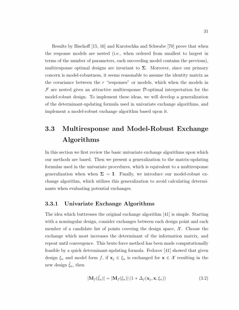
31
Results by Bischoff [15, 16] and Kurotschka and Schwabe [70] prove that when
the response models are nested (i.e., when ordered from smallest to largest in
terms of the number of parameters, each succeeding model contains the previous),
multiresponse optimal designs are invariant to Σ. Moreover, since our primary
concern is model-robustness, it seems reasonable to assume the identity matrix as
the covariance between the r “responses” or models, which when the models in
F are nested gives an attractive multiresponse D-optimal interpretation for the
model-robust design. To implement these ideas, we will develop a generalization
of the determinant-updating formula used in univariate exchange algorithms, and
implement a model-robust exchange algorithm based upon it.
3.3 Multiresponse and Model-Robust Exchange
Algorithms
In this section we first review the basic univariate exchange algorithms upon which
our methods are based. Then we present a generalization to the matrix-updating
formulas used in the univariate procedures, which is equivalent to a multiresponse
generalization when when Σ = I. Finally, we introduce our model-robust ex-
change algorithm, which utilizes this generalization to avoid calculating determi-
nants when evaluating potential exchanges.
3.3.1 Univariate Exchange Algorithms
The idea which buttresses the original exchange algorithm [41] is simple. Starting
with a nonsingular design, consider exchanges between each design point and each
member of a candidate list of points covering the design space, X . Choose the
exchange which most increases the determinant of the information matrix, and
repeat until convergence. This brute force method has been made computationally
feasible by a quick determinant-updating formula. Fedorov [41] showed that given
design ξn and model form f , if xj ∈ ξn is exchanged for x ∈ X resulting in the
new design ξn, then
|Mf (ξn)| = |Mf (ξn)| (1 + ∆f (xj,x, ξn)) (3.2)

32
where
∆f (xj,x, ξn) = Vf (x, ξn)−Vf (x, ξn)Vf (xj, ξn)+V2f (x,xj, ξn)−Vf (xj, ξn) (3.3)
under the assumption that σ2 = 1, with
Vf (x, ξn) = f′(x)M−1
f f(x)
and
Vf (x,xj, ξn) = f′(x)M−1
f f(xj).
We can also update the inverse of the information matrix using Lemma 3.3.1
in Fedorov [41] (using notation from Meyer and Nachtsheim [77]):
M−1f (ξn) = M−1
f (ξn)−M−1f (ξn)F1(I2 + F
′
2M−1f (ξn)F1)−1F
′
2M−1f (ξn) (3.4)
with F1 = [f(x),−f(xj)] and F2 = [f(x), f(xj)]. The Fedorov algorithm is as
follows:
1. Initialize algorithm: Begin with a nonsingular design; construct grid, C ⊂ X
2. Let j = 1.
3. For design point xj, calculate ∆(xj,x, ξn) as in (3.3) for all x ∈ C. Choose
x∗j = arg maxx∈χ ∆(xj,x, ξn).
4. Increment j and if j < n return to Step 3. Else choose
j∗ = arg maxj∈1,··· ,n
∆(xj,x∗j , ξn),
exchange xj∗ and x∗j∗ , and update the determinant.
5. Update the inverse of the information matrix according to (3.4).
6. If ∆(xj∗ ,x∗j∗ , ξn) < ε, STOP. Else return to Step 2.
This algorithm generates a convergent nondecreasing sequence of determinants,
but will not in general converge to the global optimum. Therefore, it is necessary
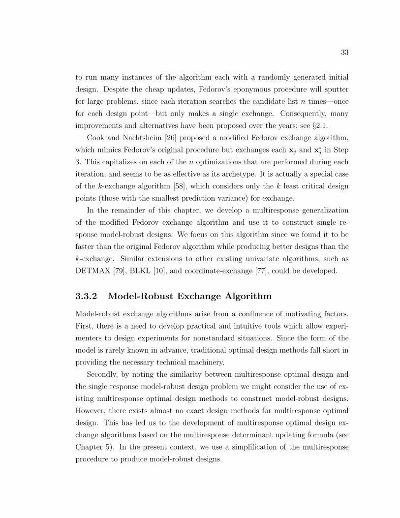
33
to run many instances of the algorithm each with a randomly generated initial
design. Despite the cheap updates, Fedorov’s eponymous procedure will sputter
for large problems, since each iteration searches the candidate list n times—once
for each design point—but only makes a single exchange. Consequently, many
improvements and alternatives have been proposed over the years; see §2.1.
Cook and Nachtsheim [26] proposed a modified Fedorov exchange algorithm,
which mimics Fedorov’s original procedure but exchanges each xj and x∗j in Step
3. This capitalizes on each of the n optimizations that are performed during each
iteration, and seems to be as effective as its archetype. It is actually a special case
of the k-exchange algorithm [58], which considers only the k least critical design
points (those with the smallest prediction variance) for exchange.
In the remainder of this chapter, we develop a multiresponse generalization
of the modified Fedorov exchange algorithm and use it to construct single re-
sponse model-robust designs. We focus on this algorithm since we found it to be
faster than the original Fedorov algorithm while producing better designs than the
k-exchange. Similar extensions to other existing univariate algorithms, such as
DETMAX [79], BLKL [10], and coordinate-exchange [77], could be developed.
3.3.2 Model-Robust Exchange Algorithm
Model-robust exchange algorithms arise from a confluence of motivating factors.
First, there is a need to develop practical and intuitive tools which allow experi-
menters to design experiments for nonstandard situations. Since the form of the
model is rarely known in advance, traditional optimal design methods fall short in
providing the necessary technical machinery.
Secondly, by noting the similarity between multiresponse optimal design and
the single response model-robust design problem we might consider the use of ex-
isting multiresponse optimal design methods to construct model-robust designs.
However, there exists almost no exact design methods for multiresponse optimal
design. This has led us to the development of multiresponse optimal design ex-
change algorithms based on the multiresponse determinant updating formula (see
Chapter 5). In the present context, we use a simplification of the multiresponse
procedure to produce model-robust designs.

34
3.3.2.1 Model-Robust Updating Formula
Recall that q is the total number of parameters in the multiresponse regression
model given in (3.1) and r is the number of responses. A multiresponse gener-
alization of the determinant updating formula (5.6) can be developed (again, see
Chapter 5) which allows the determinant of the q × q multiresponse information
matrix to be updated by evaluating the determinant of a 2r × 2r matrix when a
single point is exchanged.
However, if we assume that Σ = Ir we can simplify this updating formula so
that the update involves only scalar quantities. It is well known that the determi-
nant of a block diagonal matrix is the product of the determinants of the blocks.
Thus,
∣∣∣Mm(ξ)∣∣∣ =
∣∣∣Z′newZnew
∣∣∣ =r∏i=1
∣∣∣X′
i,newXi,new
∣∣∣=
r∏i=1
∣∣∣X′
iXi
∣∣∣ · (1 + ∆i(xj,x)) (3.5)
where Znew is the multiresponse expanded design matrix for post-exchange design
ξ, Xi,new is the univariate expanded design matrix for model i and ξ, Xi is the
univariate expanded design matrix for model i and the pre-exchange design ξ, and
∆i is as in (3.3). The last equality follows from the univariate identity (3.2). This
allows us to update the information matrix via (3.5), a scalar. We are now prepared
to describe the proposed model-robust modified Fedorov exchange algorithm.
3.3.2.2 Model-Robust Modified Fedorov Exchange Algorithm
As in Lauter [71] we consider, instead of a single model, a finite set of possible
models, F . More specifically, let ξn be an n-point design and Mi(ξn) be the
information matrix for model i where fi ∈ F , i = 1, · · · , r. Suppose that we
exchange a design point xj for an arbitrary point x in the design region, resulting
in a new design ξn. Then the model-robust optimization criteria can be written
as:
φ(MF(ξn)) =r∏i=1
∣∣∣Mi(ξn)∣∣∣ (3.6)

35
=r∏i=1
|Mi(ξn)| (1 + ∆i(xj,x))
= φ(Mf (ξn))r∏i=1
(1 + ∆i(xj,x))
so that for each iteration of the algorithm, we need to just calculate and maximize∏ri=1(1+∆i(xj,x)) where ∆i is calculated as in (3.3) for model i. We make a slight
adjustment to this criterion so our algorithm will not choose to exchange a point
that is so bad that (1 + ∆i(xj,x)) < 0 for an even number of models, which would
result in a positive value of our criterion even though the exchange is undesirable.
Thus, we choose the exchange which maximizes
r∏i=1
(1 + ∆i(xj,x))I(1 + ∆i(xj,x) > 0) (3.7)
where I is the indicator function. By (3.5) this is equivalent to updating the
multiresponse information matrix under the assumption that Σ = I.
Based on the above development, the algorithm is as follows:
1. Initialize algorithm: Begin with a nonsingular design ξn; construct grid, C ⊂X .
2. Let j = 1.
3. For design point xj, calculate (3.7) for all x ∈ C. Choose
x∗j = arg maxx∈χ
r∏i=1
(1 + ∆i(xj,x))I(1 + ∆i(xj,x) > 0).
4. Perform exchange x∗j for xj, updating ξn. Update the determinant and also(X′iXi
)−1for each model using (3.4).
5. Increment j and if j < n return to Step 3. Else, if
maxj
r∏i=1
(1 + ∆i(xj,x∗j)) < 1 + ε,
STOP. Else return to Step 2.

36
As in the univariate algorithm, to find a global optimum for larger problems it
is necessary to perform many runs of the algorithm using different initial designs.
We use ε = 0.01 for the convergence parameter.
3.4 Examples
In this section we present several examples illustrating the proposed model-robust
modified Fedorov (MRMF) exchange algorithm, and compare it with two other
exact model-robust design methods in the literature. Before giving the examples,
we briefly describe these methods and discuss how the designs will be evaluated.
DuMouchel and Jones [37] use a Bayesian approach to provide protection
against higher-order terms. They set s1 terms as primary and s2 terms as potential
and after scaling the two groups to make them nearly orthogonal, they assume an
informative prior for the potential terms and calculate a posterior distribution for
the parameters with variance A = [X′X + K/κ2]−1, where X = (Xpri|Xpot) and
K is a (s1 + s2)× (s1 + s2) diagonal matrix with 0 on the first s1 diagonals and 1
on the last s2. The prior variance parameter, κ, is to be chosen by the user. Then,
they simply choose the design that minimizes |A| using straightforward alterations
to existing exchange algorithms.
A distinct advantage of this method is that it can provide protection against
models with more parameters than observations. On the other hand, it is not
designed to produce model-robust designs with respect to more than two models.
Since it is a prominent model-robust technique for exact designs, we compare its
results to ours. Difficulties associated with this method are the choice of the prior
precision value, 1κ, and how to designate the primary and potential terms. We use
1κ
= 1, as recommended by DuMouchel and Jones, but also include designs based
upon 1κ
= 16. Because of the structure of A, larger prior precision values will result
in less consideration of the potential terms as manifested by lower efficiencies for
models involving those terms. We also generally assume more primary terms as
opposed to less. The results are based upon the implementation of this method in
the SASr software’s PROC OPTEX [92].
Heredia-Langner et al. [54] use a genetic algorithm to calculate exact model-
robust designs. They consider r possible models and optimize a desirability func-

37
tion which incorporates the determinants of the information matrices of each of the
models. Their procedure does not require a candidate list, though implementation
of a tuned genetic algorithm is not trivial. Examples in §3.4.1 and §3.4.3 are taken
from their paper, which allows comparisons to be made.
We compare designs on the basis of D-efficiencies with respect to each model
f ∈ F . The D-efficiency for model f is Df =(|Mf ||M∗f |
)1/p
where M∗f is the informa-
tion matrix for the design optimal for f alone, and p is the number of parameters
for model f . Since determinants can roughly be viewed as measures of volume,
this quantity takes the ratio of the volumes and scales the comparison to a per-
parameter basis.
For the individual model optimal designs in all examples save the last, Fe-
dorov’s algorithm via PROC OPTEX was run 50 times from randomly chosen
initial designs and the best final design was chosen. For the final example, the
MRMF algorithm was used to find the best designs for the models individually.
Furthermore, all model-robust designs produced by the methods in this chapter,
as well as those based upon the Bayesian procedure [37], were also generated based
on 50 separate algorithm instances.
All designs referred to in the following examples are given in Appendix A.
Matlabr (Version 7.8) code can be found at http://www.stat.psu.edu/~jlr/
pub/Smucker/.
3.4.1 Constrained Response Surface Experiment
A constrained two-factor example, taken from Heredia-Langner et al. [54], will
serve as an initial example illustrating our method. The design region, shown in
Figure 3.1, is X = x = (x1, x2) : −1 ≤ x1, x2 ≤ 1, x1 + x2 ≤ 1,−0.5 ≤ x1 + x2with n = 6. The experimenter would like a design robust for a first-order, a first-
order with interaction, and full quadratic polynomial; i.e. F = f ′i (x)βi, 1 ≤ i ≤3,x ∈ X where
f′
1(x) = (1, x1, x2) (3.8)
f′
2(x) = (1, x1, x2, x1x2) (3.9)
f′
3(x) = (1, x1, x2, x1x2, x21, x
22) (3.10)

38
The candidate list for this example consisted of 266 points constituting a grid
of resolution 0.1 placed over the design space. For the Bayesian method, we adopt1κ
= 1 and assign f′pri = (1, x1, x2, x1x2) and f
′pot = (x2
1, x22) in accordance with
recommendations in DuMouchel and Jones. We also include in our comparison
the model-robust design of Heredia-Langner et al. [54] as well as the optimal
design for the largest model.
The model-robust designs are given in Tables A.1-A.3 in Appendix A and are
shown graphically in Figure 3.1. Three design points are common to all four
designs, (0, 1), (1, 0), (1,−1), and the MRMF and Bayes methods produced the
same design. Table 3.1 also compares the designs in terms of the determinant
and D-efficiency for each of the considered models, and the last column gives the
product of the determinants and efficiencies. The last row gives the determinant of
the information matrix for the D-optimal design for each of the models individually
(see Tables A.3-A.5 in Appendix A), and the efficiencies are calculated using these
values.
−1 −0.5 0 0.5 1−1
−0.8
−0.6
−0.4
−0.2
0
0.2
0.4
0.6
0.8
1
x1
x2
Genetic AlgorithmBayes and MRMFOptimal Design for Quadratic
Figure 3.1. Model-robust designs for example in §3.4.1
Even though the Bayesian and MRMF designs seem close to the optimal de-
sign for the quadratic model (since their D-efficiency for the quadratic model is
nearly 1), the individually optimal design produces a poor efficiency with respect
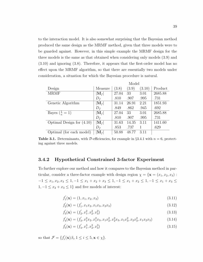
39
to the interaction model. It is also somewhat surprising that the Bayesian method
produced the same design as the MRMF method, given that three models were to
be guarded against. However, in this simple example the MRMF design for the
three models is the same as that obtained when considering only models (3.9) and
(3.10) and ignoring (3.8). Therefore, it appears that the first-order model has no
effect upon the MRMF algorithm, so that there are essentially two models under
consideration, a situation for which the Bayesian procedure is natural.
ModelDesign Measure (3.8) (3.9) (3.10) ProductMRMF |Mf | 27.04 33 3.01 2685.88
Df .810 .907 .995 .731Genetic Algorithm |Mf | 31.14 26.91 2.21 1851.93
Df .849 .862 .945 .692Bayes ( 1
κ= 1) |Mf | 27.04 33 3.01 2685.88
Df .810 .907 .995 .731Optimal Design for (4.10) |Mf | 31.63 14.35 3.11 1411.60
Df .853 .737 1 .629Optimal (for each model) |Mf | 50.88 48.77 3.11
Table 3.1. Determinants, with D-efficiencies, for example in §3.4.1 with n = 6, protect-ing against three models.
3.4.2 Hypothetical Constrained 3-factor Experiment
To further explore our method and how it compares to the Bayesian method in par-
ticular, consider a three-factor example with design region χ = x = (x1, x2, x3) :
−1 ≤ x1, x2, x3 ≤ 1,−1 ≤ x1 + x2 + x3 ≤ 1,−1 ≤ x1 + x2 ≤ 1,−1 ≤ x1 + x3 ≤1,−1 ≤ x2 + x3 ≤ 1 and five models of interest:
f′
1(x) = (1, x1, x2, x3) (3.11)
f′
2(x) = (f′
1, x1x2, x1x3, x2x3) (3.12)
f′
3(x) = (f′
2, x21, x
22, x
23) (3.13)
f′
4(x) = (f′
3, x21x2, x
21x3, x1x
22, x
22x3, x1x
23, x2x
23, x1x2x3) (3.14)
f′
5(x) = (f′
4, x31, x
32, x
33) (3.15)
so that F = f ′i (x)βi, 1 ≤ i ≤ 5,x ∈ χ.

40
In particular, assume that the experimenter would like to use n = 20 runs
and would like a design that can fit each of these models well. To specify the
Bayesian procedure, we take as primary all terms in (3.13) and designate the rest
as potential. We give the MRMF design in Table 3.2, as well as Bayesian designs
with 1κ
= 1 and 1κ
= 16 and the optimal design for the largest model, all using
a candidate list consisting of a grid of points with resolution 0.1 placed over the
design space.
The Bayesian designs are competitive for most of the models, but the designs
lack efficiency for model (3.14) when compared to the MRMF design, which might
be expected since it is in between the primary and full model and as such not
explicitly considered. None of the designs perform very well for model (3.12),
though the MRMF design is marginally better. As we expect, when a larger
prior precision value is used in the Bayesian procedure, the efficiency of models
containing primary terms is reduced, and in this case significantly degrades the
design in terms of the product criterion. The optimal design for the largest model
is competitive with the Bayesian designs in terms of model-robustness, though the
MRMF design would likely be preferred because of its higher efficiencies in models
(3.12), (3.13), and (3.14).

41
Model
Des
ign
Mea
sure
(3.1
1)(3
.12)
(3.1
3)(3
.14)
(3.1
5)P
roduct
MR
MF
|Mf|
6.58
e35.
57e4
1.10
e53.
21e0
5.24
e-3
6.78
e11
Df
.864
.756
.870
.955
.979
.531
Bay
es(
1 κ=
1)|M
f|
6.63
e35.
21e4
9.74
e49.
92e-
17.
94e-
32.
65e1
1Df
.867
.749
.860
.892
.999
.498
Bay
es(
1 κ=
16)
|Mf|
5.93
e34.
39e4
1.12
e54.
61e-
14.
41e-
35.
93e1
0Df
.843
.731
.872
.852
.970
.444
Opti
mal
for
(3.1
5)|M
f|
6.44
e34.
94e4
9.62
e47.
63e-
18.
07e-
31.
88e1
1Df
.860
.744
.859
.878
1.4
826
Opti
mal
(for
each
model
)|M
f|
1.18
e43.
93e5
4.42
e56.
97e0
8.07
e-3
Tab
le3.
2.D
eter
min
ants
,w
ithD
-effi
cien
cies
,fo
rex
ampl
ein§3
.4.2
wit
hn
=20
,pr
otec
ting
agai
nst
five
mod
els.

42
3.4.3 Constrained Mixture Experiment
We now revisit the example briefly described at the outset. This is a four-factor
constrained mixture experiment regarding the formulation of a household product
in which 20 runs are available. The design region can be defined by:
X =
x = (x1, x2, x3, x4) :
4∑i=1
xi = 1, .5 ≤ x1 ≤ 1, 0 ≤ x2, x3 ≤ .5, 0 ≤ x4 ≤ .05
where x1 is a nonionic surfactant, x2 is an anionic surfactant, x3 is a second nonionic
surfactant, and x4 is a zwitterionic surfactant. Because of the dependency induced
by the mixture constraint, standard mixture design models are considered which
do not include an intercept:
f′
1(x) = (x1, x2, x3, x4) (3.16)
f′
2(x) = (f′
1, xixj, i < j ≤ 4) (3.17)
f′
3(x) = (f′
2, xixjxk, i < j < k ≤ 4) (3.18)
f′
4(x) = (f′
3, xixj(xi − xj), i < j ≤ 4) (3.19)
so that F = f ′i (x)βi, 1 ≤ i ≤ 4,x ∈ χ. Heredia-Langner et al. [54] also used this
example, and so we compare our method to their Genetic Algorithm as well as to
the Bayesian method of DuMouchel and Jones [37]. For the latter, we use both a
standard value for the prior precision, 1κ
= 1, and a larger value, 1κ
= 16, with all
terms primary except those unique to f4, which are regarded as potential.
Since this is a large mixture design, we supplemented a regular grid (resolution
0.01) with extreme vertices and approximate centroids of the design region using
code as described by Piepel [85].

43
Model
Des
ign
Mea
sure
(3.1
6)(3
.17)
(3.1
8)(3
.19)
Pro
duct
MR
MF
|Mf|
5.31
e-2
7.22
e-22
2.65
e-43
8.36
e-78
8.49
e-14
3Df
.728
.897
.931
.996
.606
Gen
etic
Alg
orit
hm
|Mf|
5.23
e-2
7.46
e-22
2.90
e-43
7.80
e-78
8.83
e-14
3Df
.725
.900
.937
.992
.607
Bay
es(
1 κ=
1)|M
f|
5.46
e-2
6.74
e-22
2.24
e-43
9.08
e-78
7.48
e-14
3Df
.733
.890
.919
1.6
00B
ayes
(1 κ
=16
)|M
f|
5.64
e-2
6.12
e-22
3.01
e-43
3.08
e-78
3.20
e-14
3Df
.739
.882
.939
.947
.580
Opti
mal
Des
ign
for
(3.1
9)|M
f|
5.46
e-2
6.74
e-22
2.24
e-43
9.08
e-78
7.48
e-14
3Df
.733
.890
.919
1.6
00O
pti
mal
(for
each
model
)|M
f|
1.89
e-1
2.15
e-21
7.26
e-43
9.08
e-78
Tab
le3.
3.D
eter
min
ants
,w
ithD
-effi
cien
cies
,fo
rex
ampl
ein§3
.4.3
wit
hn
=20
,pr
otec
ting
agai
nst
four
mod
els.

44
In Table 3.3, the MRMF method can be seen to be competitive with the Ge-
netic Algorithm, though their design is slightly superior by our product optimality
criterion. This is likely a function of the discretization in our candidate list. Note
that the optimal design for model (3.19) alone has a significantly higher objective
function value (9.08e-78) than that given in Heredia-Langner et al. [54] (7.83e-78),
though theirs was asserted to have been obtained from PROC OPTEX in SAS as
well.
It is the case again in this example that the best design found by the MRMF
method is relatively close to that of the optimal design for the largest model. The
Bayesian design with precision of 1 actually chooses the optimal design for the
largest model, and shows that this design is competitive with those that look to
maximize the product of the determinants. When the precision is increased, we see
the same behavior as was noted before: The Bayesian design becomes less efficient
for the model that involves potential terms. The resulting Bayesian design gives
slightly more balance, but suffers against the product optimality criterion.
3.4.4 Mixture Experiment with Disparate Models
For our final example we use an unconstrained mixture experiment by Frisbee and
McGinity [42] with n = 11. The response is the glass transition temperature of
a certain film with three nonionic surfactant factors. The goal was to minimize
this transition temperature, and Frisbee and McGinity fit a traditional polynomial
model. However, another class of models, the so-called Becker models [29, Sec.
6.5], were shown by Rajagopal and Castillo [89] to also fit the data well and lead
to a significantly different optimal solution. These models, originally considered to
address certain shortcomings in the Sheffe polynomial models, use min(·) instead
of prod(·) to model second order mixture blending.
In this case,
X =
x = (x1, x2, x3) :
3∑i=1
xi = 1, 0 ≤ xi ≤ 1, i = 1, 2, 3
45
and we take five possible models:
f′
1(x) = (xi, i = 1, 2, 3) (3.20)
f′
2(x) = (f′
1, xixj, i < j ≤ 3) (3.21)
f′
3(x) = (f′
2, x1x2x3) (3.22)
f′
4(x) = (f′
1, min(xi, xj), i < j ≤ 3) (3.23)
f′
5(x) = (f′
4, min(x1, x2, x3)) (3.24)
so that F = f ′i (x)βi, 1 ≤ i ≤ 5,x ∈ X.In addition to the five models we are guarding against, we also examine effec-
tiveness of our design with respect to the model fit by Frisbee and McGinity, as
well as the most probable model found a posteriori by Rajagopal and Castillo,
respectively:
f′
fm(x) = (x1, x2, x3, x1x3, x2x3) (3.25)
f′
rc(x) = (x1, x2, x3,min(x1, x3),min(x2, x3)) (3.26)
For a candidate list, we used a regular grid with resolution 1/12, which because
of the regular design region, contained the vertices and centroids of the region.
With the disparate model types, the Bayes procedure, with its primary and
potential factors, cannot be easily applied. Instead, we examine the results of the
MRMF design and compare it in Table 3.4 to the design that was actually used.
In terms of efficiency, the design used by Frisbee and McGinity is much inferior
for all models considered because it includes, in addition to two centroid points,
three other points on the interior of the simplex design region.
As seen in Table 3.4, the MRMF design is optimal for models (3.22), (3.23),
and (3.24). This is because the optimal designs for these models individually are
interchangeable; i.e. the optimal design for one is also optimal for another. Note
that since the models are not nested we do not have the multiresponse D-optimality
interpretation.

46
Model
Des
ign
Mea
sure
(3.2
0)(3
.21)
(3.2
2)(3
.23)
(3.2
4)(4
.20)
(4.2
1)M
RM
F|M
f|
19.8
15.
91e-
35.
36e-
60.
569
2.78
e-2
6.61
e-2
1.46
Df
.745
.954
11
1.8
12.8
66F
risb
eean
dM
cGin
ity
|Mf|
8.25
1.22
e-3
1.51
e-6
.146
8.82
e-3
2.30
e-2
.588
Df
.556
.733
.835
.797
.849
.658
.722
Opti
mal
(for
each
model
)|M
f|
487.
8e-3
5.36
e-6
.569
2.78
e-2
.188
3
Tab
le3.
4.D
eter
min
ants
,w
ithD
-effi
cien
cies
,fo
rex
ampl
ein§3
.4.4
,w
ithn
=11
,pr
otec
ting
agai
nst
five
mod
els.

47
3.5 Discussion
The Model-Robust Modified Fedorov (MRMF) exchange algorithm presented in
this chapter provides a natural tool with which to find designs when an optimal
design is desired but the model-form is unknown. The mechanism to achieve
this is intuitive and simple: The experimenter chooses r models for which he/she
would like to design. Then, a design is found which maximizes the product of
the determinant of the information matrices of each of the models. In the case
that the models under consideration are nested, this is the D-optimal design for
the associated multiresponse model with r responses and thus, under normality,
minimizes the volume of the confidence ellipsoid of the parameters.
Furthermore, the MRMF method produces designs that are competitive, with
simpler algorithmic machinery, than the Genetic Algorithm (GA) approach of
Heredia-Langner et al. [54]. The strength of the MRMF method with respect
to the GA technique is that it is automatic and a straightforward extension of
commonly used exchange algorithms. The GA requires tuning of several parame-
ters and is nontrivial to implement effectively.
We also compared our procedure to the Bayesian method of DuMouchel and
Jones [37], a widely available model-robust technique. We initially hypothesized
that the Bayesian method would suffer when confronted with multiple possible
models, since it categorizes terms into just two groups. This is supported by
the second example, though the procedure performed well in the first and third
examples. The choice of 1κ
certainly affects the model-robustness of the design;
indeed for certain values of 1κ
(i.e. 1κ
= 1 in the third example) the method seems
to produce a design optimal for the highest-order model, while for large enough
values of 1κ
the full model is not even estimable. The choice of terms as primary
or potential also makes an impact. Our procedure does not suffer from these
uncertainties, has a multiresponse D-optimal interpretation (for F nested) and
explicitly considers a larger class of models; it can also handle situations as in
Example 4 in which the possible models are disparate and impossible to nest.
One strategy, if faced with a situation necessitating a D-optimal design, might
be to design for the highest-order model possible. If, as assumed in this disserta-
tion, there are a sufficient number of runs to estimate the largest model, one might

48
question whether the efficiency gained using model-robust methods is worth the
additional methodology. In certain cases, as in the third example, the gains appear
to be limited. But as demonstrated by the first and second examples, significant
gains can be made by utilizing the model-robust approach. Therefore, a dedicated
procedure based upon accepted univariate exchange algorithms will be useful to
produce model-robust designs.
In terms of D-efficiency, the MRMF designs seem to favor larger models. In
other words, the efficiency of the smaller models suffer as compared to the larger
ones. To mitigate this, one might consider the following optimization criterion
[10, 38], instead of (3.6):
φ(MF(ξn)) =r∏i=1
∣∣∣Mi(ξn)∣∣∣1/qi (3.27)
where qi is the number of parameters in the ith model. It is straightforward to
derive an exchange algorithm using this criterion–call it the scaled MRMF–which
has the effect of shrinking values of dissimilar orders of magnitude toward each
other, in essence weighting more heavily those models with fewer parameters. We
implemented this procedure using several examples, and the results were surpris-
ingly similar to the unscaled MRMF. For instance, for the constrained mixture
experiment in the third example, the scaled MRMF design resulted in a design
very close to the MRMF in Table 3.3. For the second example in §3.4.2, the scaled
MRMF design produced more of a difference, with D-efficiencies increasing from
86.4% to about 89% for model (3.11) and from 75.6% to about 78% for model
(3.12), while decreasing the efficiencies of model (3.13) from 87% to about 85.5%
and model (3.15) from 97.9% to about 96.5%. In any case, the scaled MRMF does
not result in dramatic changes in efficiency.
The model-robust criterion used in this chapter could easily be extended to
include prior information in terms of model weights, if certain models are preferred
over the others. However, since this work was motivated in part by multiresponse
optimal design theory, the minimal volume of the parameter confidence ellipsoid
interpretation of D-optimality is used and thus we only consider equally weighted
models. Furthermore, the relative ineffectiveness of the scaled MRMF to provide
designs with balanced D-efficiencies underscores the difficulty in balancing the

49
designs using weights.
Finally, assume that Te is the time it takes to run the univariate exchange
algorithm. The runtime for these model-robust algorithms should be rTe where
r is the number of models considered. Commercial software programs have fast
implementations of exchange algorithms, so the computational burden imposed by
a similarly implemented model-robust exchange algorithm should not be heavy.

Chapter 4A Maximin Model-Robust Exchange
Algorithm and its Generalization to
Include Model Preferences
In the previous chapter, we considered a model-robust procedure for an experimen-
tal scenario in which we allow the specification of multiple models and a maximiza-
tion of the product of the determinant of the information matrices with respect to
these models. In this chapter, we stay within the same model-set framework, but
maximize the minimum D-efficiency.
4.1 Introduction
Again, assume that an experiment is to be designed for which there is a single
response and k factors of interest. As before, the linear regression model y = Xβ+ε
will be fit, where y is an n-vector of independent observations, X is the n × p
expanded design matrix, β is the p × 1 vector of unknown parameters, and ε is
also an n-vector with E(ε) = 0 and V ar(ε) = σ2. Assume also that the classical
least squares criterion will be used to estimate β, in which case the estimator is
β = (X′X)−1X′Y with V ar(β) = σ2(X′X)−1. Recall that the inverse of V ar(β)
is called the information matrix, denoted as M = (X′X)/σ2 = [V ar(β)]−1.
Furthermore, we again let X be the design space, Ξ be the set of all possible

51
designs and ξn ∈ Ξ be a discrete, n-point design which can be represented as
ξn =
(x1 x2 . . . xd
n1 n2 . . . nd
)(4.1)
where n =∑d
i=1 ni is the total number of experiments, and ni is the number of
experiments performed at design point xi, i = 1, . . . , d.
An optimal design strategy chooses a design by optimizing a function of the
information matrix. The D-criterion maximizes φ(M) = |M|, which is equivalent
to minimizing the volume of the confidence ellipsoid about the parameter estimates
if normality is assumed.
Implicit in the structure of X is the design, ξn, as well as a model form, f(x),
which is a p × 1 expanded design vector that is usually assumed given though
in reality is rarely known. Consequently, we represent the information matrix
as Mf (ξn), though we may express it as Mf in the interest of simplicity. Thus,
φ(Mf (ξn)) depends upon the model form f and an optimal design for one model
is not in general optimal for another. To mitigate against an undue reliance upon
a single model form f , we again allow a user-chosen set of models, F .
In our experience the model-robust procedures which use a form ofD-optimality
(such as our procedure in Chapter 3, the Genetic Algorithm approach of Heredia-
Langner et al. [54], and the Bayesian approach of DuMouchel and Jones [37])
often produce designs which have high D-efficiencies for some models (generally
those with the most parameters), but considerably lower D-efficiencies for others.
Furthermore, these algorithms give experimenters little a priori control over the
efficiencies of the design with respect to the given possible models and indeed
exhibit a substantial lack of efficiency balance across them. Efficiency balance,
which we formally define in §4.3, occurs when a design has the same efficiency
with respect to each model in a specified set.
We propose a maximin model-robust exchange algorithm which gives exact
designs with substantially more balance than those from the aforementioned pro-
cedures, while optimizing the worst-case efficiency with respect to a user-specified
set of models. We develop a generalization of this algorithm which allows the spec-
ification of model interest levels (weights), providing additional control over the
52
D-efficiencies with respect to each model. Though the procedure is explicitly for
finite run sizes, we explore some asymptotic properties of this generalized maximin
criterion, showing that even if there is not perfect balance among the efficiencies
of all models, there will be among a subset of at least two models. We also specify
a condition which guarantees complete asymptotic efficiency balance among all
models in F .
Several authors have studied a similar criterion. For instance, Imhof and Wong
[57] give a graphical method to find asymptotic maximin designs when two dif-
ferent optimality criteria are used. Dette and Franke [33] explicitly characterize
continuous maximin designs in the specific case of polynomial regression on [−1, 1],
where they maximize the minimum efficiency with respect to possible polynomial
models as well as a goodness-of-fit criterion. Berger and Tan [11] use the maximin
criterion for mixed effects models. In contrast, the motivation for our work in this
chapter is to provide a useful, flexible tool for experimenters to construct exact
model-robust designs, for completely randomized experiments, for general design
spaces and small run sizes, allowing the user to specify a class of possible models
and exert as much control as possible over the design performance with respect
to each. The continuous design results in this chapter are an almost incidental
consequence of our observations of the discrete procedure’s performance, and we
will show empirically that even small run sizes exhibit similar behavior.
The chapter is arranged as follows. In the next section, we describe classic
exchange algorithms for D-optimality, and then present our generalized maximin
procedure. Following that, we give some results concerning the balance properties
of this criterion, though here we resort to continuous design theory. We then
present several examples illustrating the exact procedure, and conclude with a
discussion.
4.2 A Generalized Maximin Model-Robust Ex-
change Algorithm
The maximin procedure we describe is built upon a classic exchange algorithm for
D-optimality. This and other such algorithms were reviewed in Chapter 3.3.1. We

53
follow our previous work and use the modified Fedorov algorithm [26] as the basis
for our model-robust procedure. The determinant and inverse of the information
matrix for a particular model f can be updated via (3.2) and (3.4).
We assume that a set of r models, F , will be chosen and explicitly formulated.
For instance, for single-factor polynomial regression, the experimenter might desire
protection for possible polynomial models of degree 1 to 4.
Furthermore, a model interest (weight) vector, v = (v1, . . . , vr) ∈ (0, 1], must
be supplied which quantifies the interest the experimenter has in each model. By
default, the model interest is unity for all models in which case the algorithm
maximizes the minimum efficiency. If certain models are less important, however,
they can be assigned lower interest levels which will often decrease their efficiencies
compared to those with larger values. We require that maxf∈F vf = 1. Note
that these model interest levels can also be framed as prior probabilities. For
instance, if there are two possible models, f1 and f2, and the model interest vector is
v = (1, 0.8), this is equivalent to specifying a prior probability of 1/(1+0.8) = 0.56
for the first model and 0.8/(1 + 0.8) = 0.44 for the second.
The algorithm also requires as input the determinant of the information matrix
of the optimal design for each model individually so that efficiencies can be cal-
culated. This is not a stringent requirement in light of the capabilities of readily
available software; for instance, the SASr software’s PROC OPTEX [92]. Finally,
the algorithm requires a user-constructed candidate list, C, of design points.
The algorithm works on efficiencies, and the most prevalent in this context is
D-efficiency. Assuming ξ∗n is the optimal design for model f , the D-efficiency for a
design ξn with respect to model f is defined as:
Df (ξn) =
(|Mf (ξn)||Mf (ξ∗n)|
)1/p
(4.2)
where Mf (ξn) is the information matrix with respect to model f and design ξn,
Mf (ξ∗n) is the information matrix for the design optimal for f alone, and p is the
number of parameters for model f . The D-efficiency roughly scales the efficiency
of a design to a per-parameter basis and the reciprocal is a factor indicating the
additional sample size required to estimate the parameters to the same level of
precision as the optimal design (note: Df (ξn) ∈ [0, 1]). In the generalized version

54
of our maximin algorithm, we define generalized D-efficiency, for model f , as
Gf (ξn) =Df (ξn)
vf(4.3)
where vf is the interest weight for model f . Note that unlike D-efficiency, Gf (ξn) ∈[0,∞).
To illustrate the utility of generalized D-efficiency, consider an experimental
situation in which there are two models of interest, f1 and f2, with a model interest
vector v = (1, .8). In this case, finding a design maximizing the minimum D-
efficiency will not reflect this prior belief. Instead, we find the maximin design
using Gf (ξn). Thus, if the current design gives Df1(ξn) = 0.85 and Df2(ξn) = 0.75,
we find that Gf1(ξn) = 0.85 and Gf2(ξn) = 0.75/v2 = 0.75/.8 = .9375 so that f1
has the lower generalized D-efficiency even though it has the larger D-efficiency.
By working on Gf (ξn) instead of Df (ξn), the model interest levels are reflected in
the D-efficiencies of the generalized maximin design.
In the algorithm, we extend the notation of (4.3) to Gf,jk(ξn) to represent
the generalized D-efficiency when the jth design point is exchanged with the kth
candidate point. The algorithm is as follows.
1. Initialize algorithm: Input optimal determinants, |M∗f |, for each f ∈ F as
well as model interest vector, v. Construct candidate list, C ⊂ X , with c
candidate points. Specify nonsingular initial design, ξn. For each model,
calculate Gf (ξn) via (4.3) and determine fmin = arg minf∈F Gf (ξn).
2. Let j = 1 (index for design points).
3. Let k = 1 (index for candidate points).
4. For design point xj and candidate point xk, calculate ∆fmin(xj,xk, ξn) as in
(3.3).
(a) If ∆fmin(xj,xk, ξn) < 0, do not consider xk for exchange because the
minimum efficiency would not be increased.
i. If k = c, go to step 5.
ii. If k < c set k = k + 1 and return to step 4.
55
(b) If ∆fmin(xj,xk, ξn) ≥ 0, calculate ∆f (xj,xk, ξn) for all f 6= fmin and
evaluate the determinant of the information matrices for each f ∈ Faccording to (3.2). Calculate the generalized efficiencies via (4.2) and
(4.3) and determine Gfmin,jk(ξn) = minf∈F Gf,jk(ξn).
i. If k = c, go to step 5.
ii. If k < c set k = k + 1 and return to step 4.
5. Exchange xj with xk∗j , where k∗j = arg maxkGfmin,jk(ξn).
6. Update M−1f for all f ∈ F using (3.4). Calculate |Mf | for all f ∈ F .
7. Set j = j+1 and if j < n return to step 3. If j = n and termination criterion
is met, STOP. If j = n and termination criterion not met, return to Step 2.
The termination criterion stops the algorithm if maxj,f∈F ∆f (xj,x∗kj, ξn) < ε,
where ε is a small, positive constant (typically ε = 0.01).
If the experimenter is interested in each model equally, this algorithm spe-
cializes to a maximin procedure which finds a design maximizing the smallest
D-efficiency. The model interest vector, however, affords the user a great deal of
flexibility because designs focusing primarily on those models of most interest can
be generated, while protection against and estimability for less likely models can
be maintained.
Though we explore some asymptotic properties of this model-robust criterion
in the following section, we have not found these properties severely compromised
in small-sample situations. In what follows, the “maximin” design or exchange
algorithm refers to the specific case in which each element of the model interest
vector is 1. “Generalized maximin” refers to possibly unequal model interest ele-
ments. Similarly, “efficiency” refers to Df , while “generalized efficiency” refers to
the efficiencies adjusted by the model interest vector as in (4.3).
4.3 Asymptotic Properties of Generalized Max-
imin Criterion
Although we believe that exact designs are most useful and relevant to experi-
menters, we can obtain insight into these maximin designs by studying their con-
56
tinuous counterparts. In what follows, we give a condition which ensures that the
generalized maximin criterion will produce designs balanced in terms of generalized
efficiencies. Technical details, and proofs of the results in this section, are given in
Appendix B.
For the purposes of this section we define an asymptotic, or continuous, de-
sign as a discrete probability measure ξ over X , which implies that there exists a
countable number of design points upon which there is positive measure. A design
defined in this way can be thought of as the proportion of the available exper-
imental budget assigned to any particular design point x in X and represented
as
ξ(x) =
(x1 x2 . . . xd
λ1 λ2 . . . λd
)(4.4)
where λi, i = 1, . . . , d is the measure on the designs points with positive measure.
The information matrix is p× p:
M(ξ) = σ−2
d∑i=1
λif(xi)f′(xi) (4.5)
Before proceeding further, we formally define generalized efficiency balance and
limiting models.
Definition 1. Given a design, ξ, along with a set of models, F , generalized effi-
ciency balance is achieved for a subset of models F ′ ⊆ F if
Gfmax(ξ)−Gfmin(ξ) = 0 (4.6)
where fmin = arg minf∈F ′ Gf (ξ), fmax = arg maxf∈F ′ Gf (ξ), and fmin 6= fmax.
Alternatively, we refer to the elements of F ′ as limiting models.
Notice that a design could have generalized efficiency balance with respect to
F , the complete set of models, in which case we say that the design has complete
generalized efficiency balance (CGEB).
The following result guarantees that the maximin design will have generalized
efficiency balance for some subset of F . In other words, a set of at least two
limiting models is sure to exist.

57
Theorem 1. Assume F has r ≥ 2 elements and let ξ∗ = arg maxξ∈Ξ minf∈F Gf (ξ)
and fmin = arg minf∈F Gf (ξ∗). Also, assume that ξ∗ is not optimal for any f ∈ F
individually. Then, Gf (ξ∗)−Gfmin
(ξ∗) = 0 for at least one f ∈ F\fmin.
We next give a condition which, if satisfied, ensures that CGEB is attained
for the continuous maximin design. Assume F is a set of models with an arbi-
trary proper subset F ′ ⊂ F , and let ξ∗ = arg maxξ∈Ξ minf∈F Gf (ξ), and ξ′
=
arg maxξ∈Ξ minf∈F ′ Gf (ξ). Then, the condition is
minf∈F ′
Gf (ξ′) > min
f∈F ′Gf (ξ
∗) (4.7)
The condition specifies, essentially, that we can do better than ξ∗ when the
set of models is a strict subset of F . While Theorem 2 shows that (4.7) is a
sufficient condition for CGEB, we know of no a priori way to check it for a given
F . Consequently, the value of the following balance theorem rests on the insight
it provides when a particular set of models does not provide balance.
Theorem 2. Assume F has r elements and satisfies (4.7). Let
ξ∗ = arg maxξ∈Ξ
minf∈F
Gf (ξ)
and fmin = arg minf∈F Gf (ξ∗). Then, Gf (ξ
∗)−Gfmin(ξ∗) = 0 ∀f ∈ F .
This result is more descriptive than prescriptive, because it produces under-
standing in the case that balance does not happen instead of showing what classes
of models achieve generalized efficiency balance. The contrapositive to Theorem
2 is that if the models do not produce balance, condition (4.7) does not hold; i.e.
for some subset or group of subsets of F , the maximin design is no better than for
F itself. This suggests a subclass of limiting models that constrain the maximin,
which is guaranteed by Theorem 1.
The final result is a special case of Theorem 2 when r = 2, and is somewhat
like a result in Imhof and Wong [57], though in a different context.
Corollary 1. Let F have just 2 elements, f1 and f2, and
ξ∗ = arg maxξ∈Ξ
minf∈F
Gf (ξ),

58
and ξ∗fibe the optimal design for model fi alone. If neither ξ∗ 6= ξ∗f1 nor ξ∗ 6= ξ∗f2,
then Gf (ξ∗)−Gfmin
(ξ∗) = 0 for f 6= fmin.
This corollary says that when the maximin design is not the same as one of
the individually optimal designs, efficiency balance (when model interest elements
are equal) is achieved when only two models are considered. This holds, too, for
generalized maximin designs, though there are nontrivial examples in which the
maximin design is the same as the optimal design for one of the models individually.
For instance, consider the situation in which we have two nested possible mod-
els, f1 and f2, with v = (0.5, 1). It is likely that the design optimal for f2 will
have a D-efficiency with respect to f1 of more than 50%, in which case Gf1 > 1.
This implies that the maximin design, ξ∗, is the same as the optimal design for f2,
ξ∗f2 . There is obviously not CGEB here, but Corollary 1 is not invalidated because
ξ∗ = ξ∗f2 .
Because we cannot check the truth of condition (4.7) for a particular experimen-
tal situation, we cannot guarantee balance of the generalized efficiencies, though
Theorem 1 guarantees balance of some subset of F in most interesting situations.
In that sense, then, we achieve balance and the higher efficiencies for the other
models are a surplus.
However, after running the generalized maximin procedure, limiting models
often suggest themselves. Consequently, it is possible that “taking” a small amount
of efficiency from one or more of these limiting models will result in a substantial
amount of “giving” to the efficiencies of the others. Therefore, a sensitivity analysis
can be performed in which the model interest entries for the limiting models are
reduced by some user-specified amount and the algorithm is rerun. The results will
likely be lower efficiencies for the original limiting models but higher efficiencies
for the others. We will explore this in the subsequent section.
4.4 Examples
In this section we present several examples illustrating the generalized maximin
model-robust design procedure. Unless otherwise noted, all designs for a given
example were constructed using the same candidate list and 50 randomly started
algorithm tries. Optimal designs for individual models were generated using SASr

59
software’s PROC OPTEX [92]. All designs referred to in the following examples
are given in Appendix C (or, for those that appear in both this chapter and the
previous, in Appendix A). Matlabr (Version 7.8) code can be found at http:
//www.stat.psu.edu/~jlr/pub/Smucker/.
4.4.1 Constrained Two-Factor Experiment
We give first a simple six run, two-factor example used in Chapter 3 as well as
Heredia-Langner et al. [54] with a constrained design region X = x = (x1, x2) :
−1 ≤ x1, x2 ≤ 1,−0.5 ≤ x1 + x2 ≤ 1. Suppose the experimenter would like to
guard against three models:
f′
1(x) = (1, x1, x2) (4.8)
f′
2(x) = (1, x1, x2, x1x2) (4.9)
f′
3(x) = (1, x1, x2, x1x2, x21, x
22) (4.10)
so that F = f ′i (x)βi, 1 ≤ i ≤ 3,x ∈ X.We use as a candidate list the points in a resolution 0.1 grid placed over X .
In Table 4.1 we give results for a D-maximin design and a generalized D-maximin
design with model interest vector v = (1, 1, .6), as well as two other model-robust
designs for comparison, the one produced by the MRMF algorithm of Chapter
3 and the one via the Genetic Algorithm (GA) approach of Heredia-Langner et
al. [54]. We also include the optimal design for the largest considered model,
representing what might be considered the default optimal design strategy. The
final row in the table gives |M| for the optimal design for each individual model.
Notice that the non-maximin designs favor the largest model in terms of D-
efficiencies. On the other hand, the D-maximin design is close to balanced among
the three models (D-efficiences of 88.9%, 89.4%, and 88.8%, respectively), and
provides a substantial increase in the worst-case efficiency (88.8% versus 81% for
the MRMF design and 84.9% for the GA design). Complete generalized efficiency
balance, in the sense of the previous section, is not achieved because of the finite
sample size. The (1, 1, .6)-D-maximin design provides some protection for the
quadratic model while allowing very high efficiencies for models (4.8) and (4.9).

60
Notice there is not even the suggestion of CGEB here, since Gf3 = 10.6· 0.721 = 1.2
while Gf1 = .951 and Gf2 = .959. It seems likely that, asymptotically, the first
two models are the limiting ones in this case.
Our algorithm can mimic other designs, which shows its flexibility. For instance,
setting v = (.8, .9, 1) gives a design equivalent in D-efficiency to the MRMF design,
and setting v = (.9, .9, 1) produces a design with almost the same efficiencies as
that from the Genetic algorithm.
ModelDesign Measure (4.8) (4.9) (4.10)D-Maximin |Mf | 35.70 31.14 1.52
Df .889 .894 .888(1, 1, .6)-D-Maximin |Mf | 43.79 41.34 0.44
Df .951 .959 .721MRMF |Mf | 27.04 33 3.01
Df .810 .907 .995Genetic Algorithm |Mf | 31.14 26.91 2.21
Df .849 .862 .945Design Optimal for (4.10) |Mf | 31.63 14.35 3.11
Df .853 .737 1Optimal (for each model) |Mf | 50.88 48.77 3.11
Table 4.1. Determinants, with D-efficiencies, for example in §4.4.1 with n = 6, protect-ing against three models.
In Figure 4.1, we give a schematic illustrating the model-robust designs in Table
4.1. The MRMF and GA designs, which are close to optimal for the quadratic
model, each place a design point near the center of the design space with the
rest on the periphery. In contrast, the D-maximin design, with a lower efficiency
for the largest model, has an interior point but places it close to the boundary,
while the (1, 1, .6)-D-maximin has none strictly inside the space. Of course, by
using the model interest vector the generalized maximin algorithm can certainly
accommodate more emphasis on the quadratic model and less on the others if
desired, which would result in an interior point.

61
−1 −0.5 0 0.5 1−1
−0.8
−0.6
−0.4
−0.2
0
0.2
0.4
0.6
0.8
1
x1
x2
Maximin(1,1,.6)−MaximinMRMFGenetic Algorithm
Figure 4.1. Model-robust designs for example in §4.4.1
4.4.2 Constrained Mixture Experiment
A constrained mixture example, originally from Snee [96], involves five mixture
factors and their effect on the formulation of a certain plastic. The five factors
were a binder (x1), cobinder (x2), plasticizer (x3), and two monomers (x4 and x5).
In addition to the mixture constraint, each component is constrained, and there
are some multicomponent constraints as well:
X = x = (x1, . . . , x5) :5∑i=1
xi = 1
0.50 ≤ x1 ≤ 0.70
0.05 ≤ x2 ≤ 0.15
0.05 ≤ x3 ≤ 0.15
0.10 ≤ x4 ≤ 0.25
0.00 ≤ x5 ≤ 0.15
0.18 ≤ x4 + x5 ≤ 0.26
0.00 ≤ x3 + x4 + x5 ≤ 0.35

62
We consider three possible models:
f′
1(x) = (xi, i = 1, . . . , 5) (4.11)
f′
2(x) = (f′
1, xixj, i < j ≤ 5) (4.12)
f′
3(x) = (f′
2, xixjxk, i < j < k ≤ 5) (4.13)
so that F = f ′i (x)βi, 1 ≤ i ≤ 3,x ∈ X. The experimental budget was n = 25
which means model f3 is saturated. For a candidate list of design points, we
utilized the extreme vertices and approximate centroids, using the code by Piepel
[85].
In Table 4.2, we include several generalized maximin designs, the MRMF de-
sign, as well as the optimal design for f3. These are compared to the |M| for
the optimal design for each individual model (note that in addition to the extreme
vertices and approximate centroid, the candidate list for these individually optimal
designs included a grid of resolution 0.01).
For the D-maximin design it appears that, asymptotically, models f1 and f3
would be limiting, both with D-efficiencies of about 87% in this finite-sample case.
This design’s minimum D-efficiency is larger than that of the other designs, though
it has lower D-efficiency with respect to models f2 and f3 when compared to other
model-robust strategies (i.e. the MRMF design or the design optimal for model
f3).
If the experimenter is willing to give up some efficiency for the first model the
algorithm could be rerun, for instance, with v = (.9, 1, 1). The results are in Table
4.2 and is nearly CGEB with a D-efficiency for f1 about 90% that of the others.
By giving up a relatively small amount for model f1, we gain substantially on the
others. Notice that this design is closer to the MRMF design.
Alternatively, suppose that the experimenter believes a priori that f2 is most
likely, but varying degrees of protection are desired for f1 and f3. Then, v =
(.9, 1, .5) might be chosen. The results in Table 4.2 suggest that the first two
models would have GEB asymptotically (Gf1 = 0.882/0.9 = 0.98 and Gf2 = 0.979,
while Gf3 = 0.507/0.5 = 1.014). Overall, it is clear that the generalized maximin
algorithm gives great flexibility for designing with respect to the specified models.
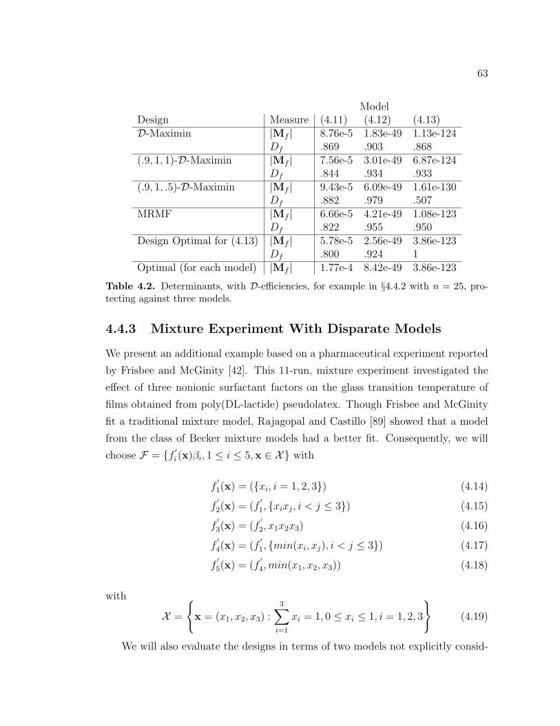
63
ModelDesign Measure (4.11) (4.12) (4.13)D-Maximin |Mf | 8.76e-5 1.83e-49 1.13e-124
Df .869 .903 .868(.9, 1, 1)-D-Maximin |Mf | 7.56e-5 3.01e-49 6.87e-124
Df .844 .934 .933(.9, 1, .5)-D-Maximin |Mf | 9.43e-5 6.09e-49 1.61e-130
Df .882 .979 .507MRMF |Mf | 6.66e-5 4.21e-49 1.08e-123
Df .822 .955 .950Design Optimal for (4.13) |Mf | 5.78e-5 2.56e-49 3.86e-123
Df .800 .924 1Optimal (for each model) |Mf | 1.77e-4 8.42e-49 3.86e-123
Table 4.2. Determinants, with D-efficiencies, for example in §4.4.2 with n = 25, pro-tecting against three models.
4.4.3 Mixture Experiment With Disparate Models
We present an additional example based on a pharmaceutical experiment reported
by Frisbee and McGinity [42]. This 11-run, mixture experiment investigated the
effect of three nonionic surfactant factors on the glass transition temperature of
films obtained from poly(DL-lactide) pseudolatex. Though Frisbee and McGinity
fit a traditional mixture model, Rajagopal and Castillo [89] showed that a model
from the class of Becker mixture models had a better fit. Consequently, we will
choose F = f ′i (x)βi, 1 ≤ i ≤ 5,x ∈ X with
f′
1(x) = (xi, i = 1, 2, 3) (4.14)
f′
2(x) = (f′
1, xixj, i < j ≤ 3) (4.15)
f′
3(x) = (f′
2, x1x2x3) (4.16)
f′
4(x) = (f′
1, min(xi, xj), i < j ≤ 3) (4.17)
f′
5(x) = (f′
4,min(x1, x2, x3)) (4.18)
with
X =
x = (x1, x2, x3) :
3∑i=1
xi = 1, 0 ≤ xi ≤ 1, i = 1, 2, 3
(4.19)
We will also evaluate the designs in terms of two models not explicitly consid-

64
ered in our model-robust design. The first is the model fit by Frisbee and McGinity,
and the second is the model found most probable a posteriori by Rajagopal and
Castillo:
f′
fm(x) = (x1, x2, x3, x1x3, x2x3) (4.20)
f′
rc(x) = (x1, x2, x3,min(x1, x3),min(x2, x3)) (4.21)
For a candidate list, we used a regular grid with resolution 1/12, which because
of the regular design region, contained its vertices and centroids.
The efficiencies for the D-maximin design are given in Table 4.3 with probable
limiting models f1 and f5 (this was confirmed by additional work in which we set
n = 50 with a denser grid). Based on this result, the experimenter might want to
generate another design in which v = (.9, 1, 1, 1, .9), which can be seen in Table 4.3
to have f1 and f4 as probable limiting models, with Gf1 = 0.883 and Gf4 = 0.888.
In this case, allowing such a sensitivity analysis produces gains for the final four
models, while degrading f1 only slightly.
Also in Table 4.3 is the MRMF design from [95] as well as the original design
of Frisbee and McGinity. For comparison purposes, we include also the optimal
designs for the two “maximal” models, f3 and f5. All designs excepting these latter
two are included in Figure 4.2.

65
Model
Des
ign
Mea
sure
(4.1
4)(4
.15)
(4.1
6)(4
.17)
(4.1
8)(4
.20)
(4.2
1)D
-Max
imin
|Mf|
24.7
33.
71e-
33.
00e-
60.
200
6.43
e-3
7.97
e-2
1.44
Df
.802
.883
.921
.840
.811
.843
.863
(.9,
1,1,
1,.9
)-D
-Max
imin
|Mf|
24.1
24.
48e-
33.
34e-
6.2
808.
14e-
37.
31e-
21.
07Df
.795
.911
.935
.888
.839
.828
.814
MR
MF
|Mf|
19.8
15.
91e-
35.
36e-
60.
569
2.78
e-2
6.61
e-2
1.46
Df
.745
.955
11
1.8
12.8
66D
esig
nO
pti
mal
for
(4.1
6)|M
f|
19.8
15.
9e-3
5.36
e-6
.569
2.78
e-2
.102
52.
15Df
.745
.955
11
1.8
86.9
36D
esig
nO
pti
mal
for
(4.1
8)|M
f|
11.5
85.
2e-3
5.36
e-6
.486
2.78
e-2
7.6e
-31.
36Df
.623
.935
1.9
741
1.8
34.8
54F
risb
eean
dM
cGin
ity
|Mf|
8.25
1.22
e-3
1.51
e-6
.146
8.82
e-3
2.30
e-2
.588
Df
.556
.733
.835
.797
.849
.658
.722
Opti
mal
(for
each
model
)|M
f|
487.
8e-3
5.36
e-6
.569
2.78
e-2
.188
3
Tab
le4.
3.D
eter
min
ants
,w
ithD
-effi
cien
cies
,fo
rex
ampl
ein§4
.4.3
wit
hn
=11
,pr
otec
ting
agai
nst
five
mod
els.

66
The results of the maximin designs are as advertised: Their minimum D-
efficiency is at least 5% higher than the others. They do, however, give up efficiency
for models f2-f5. We note that choosing v = (.75, 1, 1, 1, 1) results in a generalized
maximin design equivalent to the MRMF or the design optimal for f3 alone. Care
must be taken when interpreting the efficiencies with respect to the fitted models,
ffm and frc. For instance, the MRMF design and the design optimal for f3 alone
appear to be equivalent, though their efficiencies for ffm and frc differ. This is
because, as seen in Figure 4.2, the MRMF design includes two design points at
(.5, .5, 0) and one at (0, .5, .5), while the design optimal for f3 alone (not shown)
has only one design point at (.5, .5, 0) and two at (0, .5, .5). Since the fitted models
include a blending term with both x2 and x3 but not one with x1 and x2, the latter
design is preferred over the former. Unless an a priori inclination for the correct
blending term exists, there is no reason to prefer one over the other at the design
stage.
4.5 Discussion
The maximin exchange algorithm presented in this chapter is a practical model-
robust procedure which produces designs robust for a set of experimenter-specified
model forms by maximizing the minimum D-efficiency with respect to each model.
It also admits specification of varying levels of interest in each model so that a
design reflective of those interests will be generated and as such affords additional
control to the user. This method provides a worst-case efficiency guarantee and in
our experience usually has a significantly higher minimum efficiency than those of
the procedures against which they were compared.
We noticed that the designs produced by this procedure tend to have less vari-
able efficiencies (with respect to the models designed for) than those from other
methods. This led to the asymptotic analysis in §4.3 which gives a condition which
guarantees complete generalized efficiency balance. This condition is often unsat-
isfied; however, we also proved that even when complete balance is unattainable,
some subset of the specified models is limiting and therefore balanced. We em-
phasize that the utility of this procedure is not dependent upon these asymptotic
results, but that they can provide insight into the algorithm and its designs.

67
Figure 4.2. Some 11-run designs for example in §4.4.3, with repeated points noted
Included in our comparisons are optimal designs for the largest model under
consideration. This represents a reasonable model-robust design strategy that
might be employed using commercially available software. This approach gives no
worst-case protection, however, which may result in unnecessarily small efficiencies
for smaller models. It also gives the experimenter no control over the efficiencies
with respect to any model besides the one that is assumed. Our maximin procedure
addresses both of these issues.
Our method can also be used similarly to the Bayesian approach of DuMouchel
and Jones [37], in which an assumed model exists but protection is desired for some
larger model. The maximin procedure allows a quantification of the required degree
of protection by assigning an appropriate model interest element. For instance,

68
if a main effects model is likely, but at least some estimation of the two-factor
interaction model as well as the full quadratic model is needed, a model interest
vector v = (1, .5, .5) could be specified and would result in a design with a high
efficiency for the main effects model, but much less for the larger models (though
still with the capacity to estimate them). If possible, the design would be CGEB,
but even if it is not, the differences in efficiency will be suggestive of v. We do note
that our procedure requires n ≥ pl, where pl is the number of parameters in the
largest model, while the Bayesian procedure eludes this restriction by using prior
information.
A near upper bound on the runtime of this algorithm is mTEx, where m is the
number of models considered, and TEx is the time taken by the classical exchange
algorithm (in the case of this chapter, the modified Fedorov algorithm). We say
“near upper bound” because there is a small amount of computational energy
expended in calculating efficiencies which is unnecessary in the classical case. In
practice, the runtime should be less than the near upper bound because exchanges
are only evaluated for all models if the exchange increases the efficiency for the
model currently with the lowest efficiency.

Chapter 5Multiresponse, Model-Robust
Experimental Design
5.1 Introduction
Many times, when an experiment is to be designed, there will be more than one
response of interest. For instance, a food scientist may want to explore the effect
of different combinations of ingredients on taste, texture, nutritional value, and
cost. Or, an engineer may examine how various levels of constituent components
of a tire tread compound affect properties such as rate of wear and hardness.
The preponderance of research in the design of experiments, however, has been
directed toward the univariate case. In the multiresponse realm, there have been
primarily theoretical advances with little guidance for practical situations. Is it
worth the extra effort inherent in methodology that explicitly accounts for multiple
responses? If so, can we develop tools that leverage multiresponse characteristics
to produce an advantage over usual practice?
There are good reasons for the relative dearth of research in optimal multire-
sponse experimental design. In general, to design such an optimal experiment the
relationship between the responses as quantified in the covariance matrix Σ must
be known a priori. Furthermore, the form of the relationship—the model form—
between each response and the factors must also be specified in advance. In the
absence of these elements, the experimenter is forced to ignore both and design for

70
an assumed but unknown single model.
We approach this problem from a model-robust perspective, and argue that in
many cases a good design is a model-robust one for which Σ is irrelevant or unim-
portant anyway. When both the model form and covariance matrix are unknown,
the multiresponse D-optimal design problem can be cast effectively as a univariate
model-robust design problem.
One contribution of this chapter is to develop and present an exchange algo-
rithm to construct multiresponse D-optimal designs when the covariance matrix
and response model forms are known. But since this information is rarely known
in practice, we extend the multiresponse model and the algorithm to allow for
the construction of a design which is robust for an experimenter-specified set of
possible models for each response.
We first review the multiresponse model, and then give an overview of our ap-
proach. Subsequently, we generalize matrix- and determinant-updating formulae
given for the univariate case by Fedorov [41], and use them in a multiresponse
exchange algorithm which assumes knowledge of both the covariance matrix and
model forms. This corresponds to the most studied and least likely practical sce-
nario for multiresponse design, so we then explore the relaxation of these assump-
tions, illustrating the methodology with several examples.
5.2 Background
The classical multivariate regression model [4] assumes the model form is common
to all responses, and it has been shown [22, 70] that in this case the multiresponse
optimal design solution is identical to the univariate optimal design. We use the
more flexible seemingly unrelated regression (SUR) model [115] which allows dif-
ferent model forms for each response.
We now review this multiresponse model. Suppose there are r responses, k
factors of interest, and n observations for each response. Let
yi = Ziβi + εi
be the linear regression for response i, with yi the n-vector of observations, Zi

71
the n× qi expanded design matrix, βi the qi × 1 vector of parameters, and εi the
n-vector of errors. Further, let q =∑
i qi. Then, this multivariate model can be
specified as y1
y2
...
yr
=
Z1 0 . . . 0
0 Z2 . . . 0...
.... . .
...
0 0 . . . Zr
β1
β2
...
βr
+
ε1
ε2
...
εr
(5.1)
or more concisely as
Y = Zβ + ε (5.2)
where Y and ε are now nr×1 vectors, β is a q×1 vector, and Z is a nr×q matrix
and all of these quantities are shown in (5.1).
We make the standard normality assumption that ε ∼ N(0,Ω) where Ω =
Σ⊗ In and ‘⊗’ is the Kronecker product. Here Σ models the covariance between
the responses and In models the assumed independence across observations within
a particular response.
An estimate for β in (5.2) is given by the generalized least squares estimator
(also known as the Aitken estimator):
β = (Z′Ω−1Z)−1Z
′Ω−1Y (5.3)
with
V ar(β) = (Z′Ω−1Z)−1
Under the assumption of normality, β is also the maximum likelihood estimator
[115]. Since Σ is usually unknown, the estimator in (5.3) cannot be employed
directly, though estimators for Σ have been proposed (see [115, 63]). We omit this
discussion because of the present focus on design.
The multiresponse design problem is to specify n design points with respect to
the aforementioned multiresponse regression model. Let X be the design space, Ξ
be the set of all possible designs and ξn(x) ∈ Ξ be a discrete, n-point design:
ξn =
(x1 x2 . . . xd
n1 n2 . . . nd
)

72
where d is the number of distinct design points, and ni, i = 1, . . . , d is the number
of runs performed at design point xi.
For this exact design we define the multiresponse information matrix:
Mm(ξn,Σ) =n∑i=1
ρ(xi)Σ−1ρ′(xi)
= Z′Ω−1Z
=[V ar(β)
]−1
where
ρ′(x) =
z′1(x) 0 . . . 0
0 z′2(x) . . . 0
......
. . ....
0 0 . . . z′r(x)
(5.4)
is an r × q matrix, and z′i(x) is a vector with entries of the same form as the
expanded design matrix Zi, for response i and design point x. The multiresponse
D-optimal design maximizes the determinant of the information matrix:
ξ∗n = arg maxξn∈Ξ
|Mm(ξn,Σ)|
Implicit in the information matrix is a dependence upon ρ(x), which includes
the model form for each response, as well as the response covariance matrix Σ.
The work in this chapter examines these assumptions and design options in the
face of them.
5.3 Model-Robust Design for the SUR Model
Similar to what has been proposed in the single response case (see, for instance,
Chapters 3 and 4, as well as [71, 26, 54]), we allow the experimenter to choose a
set of potential model forms, Fi, for each response i, where each set has pi models.
What follows is an artificial, admittedly byzantine exercise meant only to establish
a structure within which model-robust designs for multiresponse experiments can
be constructed.

73
For the purposes of model-robust design, imagine a multiresponse model which
has, instead of r responses as described above, p =∑r
i=1 pi responses, one for
each possible model form assigned to each response. To specify such a framework,
we let y`j be an n-vector of observations for response ` and potential model j.
Then, all of the “data” for response ` is an np`-vector, Y` = (y′
`1, . . . ,y′
`p`)′
and
Y = (Y1, . . . ,Yr)′
is an np-vector. Further, let Z`j be the n× q`j expanded design
matrix for response ` and model j, where q`j is the number of parameters and∑r`=1
∑p`
j=1 q`j = q. Then, we have the SUR model
y11
...
y1p1
y21
...
y2p2...
yr1...
yrpr
=
Z11 . . . 0 0 . . . 0 . . . 0 . . . 0...
. . ....
......
......
......
...
0 . . . Z1p1 0 . . . 0 . . . 0 . . . 0
0 . . . 0 Z21 . . . 0 . . . 0 . . . 0...
......
.... . .
......
......
...
0 . . . 0 0 . . . Z2p2 . . . 0 . . . 0...
......
......
.... . .
......
...
0 . . . 0 0 . . . 0 . . . Zr1 . . . 0...
......
......
......
.... . .
...
0 . . . 0 0 . . . 0 . . . 0 . . . Zrpr
β11
...
β1p1
β21
...
β2p1...
βr1...
βrpr
+
ε11
...
ε1p1
ε21
...
ε2p2...
εr1...
εrpr
where β`j is a q`j × 1 vector, and y`j and ε`j are n× 1 vectors. This model can be
written more succinctly as
Y = Zβ + ε (5.5)
where Y and ε are np-vectors, Z is an np × q matrix, and β is a q-vector.
Suppose we further make the distributional assumption that ε has mean 0 and
np × np covariance matrix Ω. Then, the information matrix is Mm(ξn, Σ) =

74
∑ni=1 ρ(x)Σ−1ρ
′(x) = Z′Ω−1Z where
ρ′(x) =
z′11(x) 0 . . . 0 . . . 0
0 z′12(x) . . . 0 . . . 0
......
. . ....
. . ....
0 0 . . . z′1p1
(x) . . . 0...
.... . .
.... . .
...
0 0 . . . 0 . . . zrpr(x)
and Σ is given (see below) with Ω = Σ⊗ In.
Note that if Ω and ρ(x) are specified, the multiresponse D-optimal design for
(5.5) will account for all model forms implicit in the SUR model. Thus, we can
relax the model-form assumption for each response by framing the model-robust
problem as a large multiresponse optimal design problem in which each response
is assigned a set of possible model forms.
Again, this is an artificial device because the design problem at hand only in-
volve r responses, not p. However, if the determinant of this expanded information
matrix is maximized, the resulting design should be robust to the models repre-
sented in Fu = F1 ∪F2 ∪ . . .∪Fr in the same way that a multiresponse D-optimal
design can give a model-robust single response design (see Chapter 3).
To utilize this idea we must specify Σ. In the expanded model, there are p
“responses” (really response/model combinations) which means Ω = Σ⊗ In where
Σ is p × p. Recall that the true response covariance matrix is Σ = σ2ij for
i, j = 1, . . . , r, and in the case that this quantity is known in advance, we must
incorporate it into Σ. Then, a reasonable specification is Σ = Σ⊗Ip, where p is the
number of possible models for each response. This is somewhat restrictive, because
the number of models must be the same for all responses; however, we found that a
more complex specification allowing the number of models to vary over responses—
that different possible models within a given response are uncorrelated, but for any
two response/model combinations ij and i′j′
so that i 6= i′
the correlation is σ2ii′
—
produced Ω not always invertible. Thus, we take Ω = Σ⊗ Ip ⊗ In.
Recall that when models are nested, multiresponse optimal designs can be
constructed in the absence of knowledge of Σ [69, 15, 16, 70]. The same results

75
suggest that for the expanded, model-robust version of the multiresponse model,
if the union of all possible models are nested, the design optimal for the expanded
model is invariant to Σ, which leads to a simplified criterion in which the present
problem is essentially the same as the one for univariate model-robustness (see
§5.4.1.2).
In summary, an artificially large SUR model can be constructed by assigning
a set of possible models to each response, and the optimal design for this larger
model is, in a sense, robust to the set of all possible models specified. In the case
that the specified possible models are nested, the best design with respect to this
large model can be found irrespective of Σ. If they are nonnested, there may be a
(usually small) loss of efficiency due to the necessity of using Σ = I.
5.3.1 Choosing a Set of Models
Optimally, when there is no preference for certain models, one would like to con-
struct a design that was robust for the set of all possible models, or the set of
all possible hierarchical models. However, the former grows exponentially in the
number of model parameters and the latter quickly grows unmanageable as well,
even for problems with as few as four or five factors.
In this section, we explore two different types of model sets for the general
case in which it is desired to provide robustness for first- and second-order terms.
We reiterate that the set of models is user-defined, and suggest these sets only
as defaults in case no preference is given to any particular first- or second-order
polynomial models. The first, which we call the SSPS (small, symmetric, pseudo-
spanning) set, uses just three models, regardless of the number of factors: main
effects; main effects and all two-factor interactions; and a full quadratic model.
The second, which we call SPS (symmetric, pseudo-spanning), scales linearly with
the number of factors (3k+3 models), and consists of the three models in SSPS as
well as
1. k models, each of which includes only a single main effect.
2. k models (for k > 2), each of which includes all main effects plus a single
two-factor interaction. The k interactions should be chosen so that each
factor shows up exactly twice.

76
3. k models, each of which includes all main effects and all two-factor interac-
tions, as well as a single quadratic term.
The term “symmetric” is used to illustrate the lack of preference for any par-
ticular factor. Furthermore, “pseudo-spanning” should not be taken in a technical
sense since it simply represents our attempt to “cover” the space of possible models.
We note that there has been recent work assigning priors to the space of possible
models [13] based on certain axiomatic assumptions, an approach discussed in the
final section of this chapter.
5.4 Design Algorithms
As stated above, there are two significant hurdles inherent in the design of optimal
multiresponse experimental designs. First, the response covariance matrix, Σ, is
often unknown at the design stage. At times, there may be historical estimates of
Σ but many experiments do not have this luxury. Secondly, the form of the model
with respect to each response is likely unavailable. A typical design gambit for the
multiresponse experimenter is to simply design for a large, assumed, univariate
model (i.e. full quadratic). This ignores, however, both of the aforementioned
issues.
In what follows, we develop an exchange algorithm to address the basic case
in which both Σ and ρ(x) are known. This, in itself, is a contribution because of
the scant literature on constructing exact designs for multiresponse experiments.
We facilitate this procedure by generalizing matrix- and determinant-updating
formulas given in the univariate case by Fedorov [41], and then discuss the model-
robust extension.
5.4.1 Basic Multiresponse Exchange Algorithm
We again base our algorithm on the modified Fedorov algorithm [26]. As in the
univariate case, we exploit updating formulae to enable the computational feasi-
bility of the multiresponse exchange algorithm In what follows, we first develop
the updating formulae, then we give the algorithm and discuss how it can be used
to find multiresponse model-robust designs.
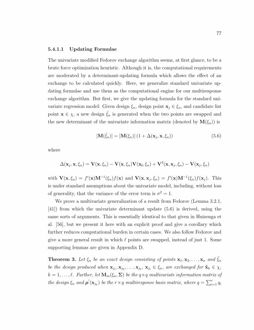
77
5.4.1.1 Updating Formulae
The univariate modified Fedorov exchange algorithm seems, at first glance, to be a
brute force optimization heuristic. Although it is, the computational requirements
are moderated by a determinant-updating formula which allows the effect of an
exchange to be calculated quickly. Here, we generalize standard univariate up-
dating formulae and use them as the computational engine for our multiresponse
exchange algorithm. But first, we give the updating formula for the standard uni-
variate regression model: Given design ξn, design point xj ∈ ξn, and candidate list
point x ∈ χ, a new design ξn is generated when the two points are swapped and
the new determinant of the univariate information matrix (denoted by M(ξn)) is
|M(ξn)| = |M(ξn)| (1 + ∆(xj,x, ξn)) (5.6)
where
∆(xj,x, ξn) = V(x, ξn)−V(x, ξn)V(xi, ξn) + V2(x,xj, ξn)−V(xj, ξn)
with V(x, ξn) = f ′(x)M−1(ξn)f(x) and V(x,xj, ξn) = f ′(x)M−1(ξn)f(xj). This
is under standard assumptions about the univariate model, including, without loss
of generality, that the variance of the error term is σ2 = 1.
We prove a multivariate generalization of a result from Fedorov (Lemma 3.2.1,
[41]) from which the univariate determinant update (5.6) is derived, using the
same sorts of arguments. This is essentially identical to that given in Huizenga et
al. [56], but we present it here with an explicit proof and give a corollary which
further reduces computational burden in certain cases. We also follow Fedorov and
give a more general result in which ` points are swapped, instead of just 1. Some
supporting lemmas are given in Appendix D.
Theorem 3. Let ξn be an exact design consisting of points x1,x2, . . . ,xn and ξn
be the design produced when xj1 ,xj2 , . . . ,xj`, xji ∈ ξn, are exchanged for xk ∈ χ,
k = 1, . . . , `. Further, let Mm(ξn,Σ) be the q×q multivariate information matrix of
the design ξn and ρ′(xjk) be the r×q multiresponse basis matrix, where q =
∑ri=1 qi

78
and qi is the number of parameters for the ith response; then
|Mm(ξn,Σ)| = |Mm(ξn,Σ)||I2`r + A′
2M−1m (ξn,Σ)A1| (5.7)
where
A1 =(−ρ(xj1)Σ
−1/2,ρ(x1)Σ−1/2, . . . ,−ρ(xj`)Σ−1/2,ρ(x`)Σ
−1/2)
and
A2 =(ρ(xj1)Σ
−1/2,ρ(x1)Σ−1/2, . . . ,ρ(xj`)Σ−1/2,ρ(x`)Σ
−1/2)
and both matrices are q × 2`r.
Proof. For brevity, we denote Mm(ξn,Σ) as Mm and Mm(ξn,Σ) as Mm.
By definition,
Mm = Mm −∑k=1
ρ(xjk)Σ−1ρ′(xjk) +
∑k=1
ρ(xk)Σ−1ρ
′(xk)
Now,
A1A′2 =
(−ρ(xj1)Σ−1/2,ρ(x1)Σ−1/2, . . . ,−ρ(xj`)Σ
−1/2,ρ(x`)Σ−1/2)
Σ−1/2ρ′(xj1)
Σ−1/2ρ′(x1)
...
Σ−1/2ρ′(xj`)
Σ−1/2ρ′(x`)
=∑k=1
−ρ(xjk)Σ−1ρ′(xjk) + ρ(xk)Σ−1ρ
′(xk)
This implies that Mm = Mm + A1A′2 and by Lemma 6 (Appendix D),
|Mm + A1A′
2| = |Mm||I2`r + A′
2M−1m A1| (5.8)
which implies what we wanted to prove.
We can generalize this further, in the case where ` = 1 and a particular
matrix is invertible. Let d(x, ξn) = ρ′(x)M−1m (ξn,Σ)ρ(x) and d(xj,x, ξn) =
ρ′(xj)M−1m (ξn,Σ)ρ(x) and x ∈ X .

79
Corollary 2. Let the setup be as in Theorem 3. Additionally, assume that ` = 1
and B = Ir −Σ−1/2d(xj, ξn)Σ−1/2 is invertible. Then
|Mm(ξn,Σ)| = |Mm(ξn,Σ)| × |B| × |Ir + Σ−1/2d(x, ξn)Σ−1/2
+ Σ−1/2d(xj,x, ξn)Σ−1/2B−1Σ−1/2d(xj,x, ξn)Σ−1/2| (5.9)
Proof. For convenience, let M−1m = M−1
m (ξn,Σ) and Mm−1
= M−1m (ξn,Σ). Since
` = 1,
A1 =(−ρ′(xj)Σ
−1/2,ρ′(x)Σ−1/2)
and
A2 =(ρ′(xj)Σ
−1/2,ρ′(x)Σ−1/2).
By Theorem 3, |Mm| = |Mm||I2r + A′2M
−1m A1|. Now,
A′
2M−1m A1 =
(Σ−1/2ρ′(xj)
Σ−1/2ρ′(x)
)M−1
m
(−Σ−1/2ρ′(xj),Σ
−1/2ρ′(x))
=
(−Σ−1/2ρ′(xj)M
−1m ρ(xj)Σ
−1/2 Σ−1/2ρ′(xj)M−1m ρ(x)Σ−1/2·
−Σ−1/2ρ′(xj)M−1m ρ(x)Σ−1/2 Σ−1/2ρ′(x)M−1
m ρ(x)Σ−1/2
)
=
(−Σ−1/2d(xj, ξn)Σ−1/2 Σ−1/2d(xj,x, ξn)Σ−1/2
−Σ−1/2d(xj,x, ξn)Σ−1/2 Σ−1/2d(x, ξn)Σ−1/2
)
Then,
|I2r + A′
2M−1m A1| =
∣∣∣∣∣ −Σ−1/2d(xj, ξn)Σ−1/2 Σ−1/2d(xj,x, ξn)Σ−1/2
−Σ−1/2d(xj,x, ξn)Σ−1/2 Σ−1/2d(x, ξn)Σ−1/2
∣∣∣∣∣= |Ir −Σ−1/2d(xj, ξn)Σ−1/2|
|Ir + Σ−1/2d(x, ξn)Σ−1/2 + Σ−1/2d(xj,x, ξn)Σ−1/2
(Ir −Σ−1/2d(xj, ξn)Σ−1/2)−1Σ−1/2d(xj,x, ξn)Σ−1/2|
where the first equality follows from Lemma 5 and the second from Lemma 4. This
implies that which we wanted to prove.

80
Theorem 3 (assuming a single exchange, i.e., ` = 1) provides computational
relief when 2r < q, and Corollary 2 reduces the burden even further, by computing
determinants and an inverse of smaller, r × r matrices.
We also would like updating formulae for the information matrix as well as
its inverse. The justification for the former is given in the proof for Theorem 3.
The proof of the latter is essentially from Fedorov [41], though it is explicitly for
a multiresponse situation.
Corollary 3. Using the assumptions of Theorem 3,
Mm(ξn,Σ) = Mm(ξn,Σ) + A1A′2 (5.10)
Theorem 4. Using the assumptions of Theorem 3,
M−1m (ξn,Σ) =
(Iq −M−1
m (ξn,Σ)A1
(I2` + A
′
2M−1m (ξn,Σ)A1
)−1
A′
2
)M−1
m (ξn,Σ)
(5.11)
Proof. First, take the inverse of both sides of (5.10) to get
M−1m = (Mm + A1A
′
2)−1 = (Iq + M−1m A1A
′
2)−1M−1m
The last equality can be verified by right multiplying both sides by Mm + A1A′2:
(Mm + A1A′
2)−1(Mm + A1A′
2) = Iq
and
(Iq + M−1m A1A
′
2)−1M−1m (Mm + A1A
′
2)
= (Iq + M−1m A1A
′
2)−1(Iq + M−1m A1A
′
2) = Iq
Then, using Lemma 7 from Appendix D, it follows that
M−1m =
(Iq + M−1
m A1A′
2
)−1
M−1m
=
(Iq −M−1
m A1
(I2` + A
′
2M−1m A1
)−1
A′
2
)M−1
m

81
5.4.1.2 Multiresponse Exchange Algorithm for D-Optimal Designs
The D-optimality criterion for the n-point multiresponse model is to maximize
φ(Mm(ξn,Σ)) = |Mm(ξn,Σ)| = |Z′Ω−1Z| = |Z′(Σ−1 ⊗ In)Z|.
However, because of the above development, when xj ∈ ξn and x ∈ X are
swapped, we have that
φ(Mm(ξn,Σ)) = φ(Mm(ξn,Σ))∆m(xj,x,Σ)
where, assuming B = Ir −Σ−1/2d(xj, ξn)Σ−1/2 is invertible,
∆m(xj,x,Σ) = |B| × |Ir + Σ−1/2d(x, ξn)Σ−1/2
+ Σ−1/2d(xj,x, ξn)Σ−1/2B−1Σ−1/2d(xj,x, ξn)Σ−1/2| (5.12)
with d(x, ξn) and d(xj,x, ξn) defined as in the prelude to Corollary 2. Otherwise,
if B−1 does not exist,
∆m(xj,x,Σ) = |I2r + A′
2M−1m (ξn,Σ)A1| (5.13)
with A1 and A2 defined as in the proof of Corollary 2. Consequently, as the
exchange algorithm considers swaps, it can choose the one which maximizes ∆m,
not φ.
If the known model forms are nested, or if Σ = Ir, it is possible to simplify φ
even further, as done in Chapter 3:
φ(Mm(ξn)) =r∏i=1
∣∣∣Mi(ξn)∣∣∣ (5.14)
=r∏i=1
|Mi(ξn)| (1 + ∆i(xj,x))
=r∏i=1
|Mi(ξn)|r∏i=1
(1 + ∆i(xj,x))

82
where Mi and ∆i are the univariate information matrices and update functions
for response model i. Then, to evaluate an exchange, we need only to calculate∏ri=1(1 + ∆i(xj,x)) where ∆i is calculated, for response i, as in (5.6).
We can make yet another simplification if some of the model forms are the
same for the different responses. Assume there are a total of R ≤ r distinct model
forms, and let td be the number of times model d appears among all the model
forms. Then we have that
r∏i=1
(1 + ∆i(xj,x)) =R∏d=1
(1 + ∆d(xj,x))td (5.15)
We make a slight adjustment to this criterion so our algorithm will not choose
an exchange so bad that (1+∆d(xj,x)) < 0 for an even td and/or an even number of
distinct models, which would result in a positive value of our criterion even though
the exchange is undesirable. Thus, we choose the exchange which maximizes
R∏d=1
(1 + ∆d(xj,x))tdI(1 + ∆d(xj,x) > 0) (5.16)
where I is the indicator function.
Based on the above development, the Multiresponse Exchange (MX) algorithm
is as follows:
1. Initialize algorithm constructing a nonsingular initial design ξn and a grid,
C ⊂ X .
2. Let j = 1.
3. For design point xj:
(a) If models are nested or Σ = I, calculate (5.16) for all x ∈ C. Let
x∗j = arg maxx∈C∏r
i=1(1 + ∆i(xj,x))I(1 + ∆i(xj,x) > 0).
(b) Otherwise, if models are not nested and Σ 6= I, calculate ∆m(xj,x,Σ),
according to (5.12) or (5.13) as appropriate, for all x ∈ C. Let x∗j =
arg maxx∈C ∆m(xj,x,Σ).

83
4. Perform exchange x∗j for xj, updating ξn. Update the determinant and also
M−1(ξn,Σ) via Theorem 4.
5. Increment j and if j < N return to Step 3. Else, if algorithm has converged,
STOP. Else return to Step 2.
The convergence criterion used here is similar to that for the algorithm in Chap-
ter ?? (ε = 0.01). This algorithm is guaranteed to converge because it produces a
bounded, nondecreasing sequence of determinants. It will not necessarily converge
to the global solution, so multiple algorithm tries using different initial designs
should be executed. Also, for large problems in particular, the determinants may
need to be calculated on the log scale.
5.4.2 Model-robust, Multiresponse Exchange Algorithm
In §5.4.1, we developed an exchange algorithm for the multiresponse model when
the response covariance matrix, Σ, and the model form of each response, ρ, are
known a priori. To extend this to the model-robust situation, for which it is
assumed that the form of the response models is not known precisely, we refer back
to §5.3 and choose a set of possible models, Fi, for each response and use them to
construct the artificial SUR model in (5.5) with covariance matrix Ω = Σ⊗Ip⊗In.
Then, the MX algorithm can be used to calculate the model-robust design.
At this point, there still is the problem of unknown Σ. However, if the choice
of possible models are such that the union of them are nested, the model-robust
design is invariant to Σ. Even for nonnested cases, our experience is that there is
little or no efficiency lost by using Σ = I (see the examples).
5.5 Examples
In this section, we demonstrate the model-robust procedures using two simple
theoretical examples, as well as a real example. All designs referred to are in
Appendix E. Matlabr (Version 7.8) code can be found at http://www.stat.psu.
edu/~jlr/pub/Smucker/.

84
5.5.1 3-factor, 2-response Experiment
The first example, used in the multiresponse design literature [112, 9], is one in
which Σ and ρ(x) are given and there is an experimental budget of n = 20 runs.
To remain consistent with previous literature, we take the design space to be
X = x = (x1, x2, x3) : −1.73 ≤ x1, x2, x3 ≤ 1.73 with known model forms, for
each response,
z′
1(x) = (1, x1, x2, x3, x1x2, x1x3, x21, x
23)
z′
2(x) = (1, x1, x2, x1x2, x21, x
22)
so that ρ′(x) =
(z′1 0
0 z′2
). We also have that the variance-covariance matrix of
the responses are
Σ =
(2 0.4
0.4 1
).
We will use the multiresponse exchange algorithm developed in §5.4.1.2 to
produce an exact solution to the multiresponse D-optimal design problem using
the given Σ and ρ. The same problem is addressed in Atashgah and Seifi [9] using
semidefinite programming, and we will compare our solution with theirs. We then
will demonstrate how the problem and solution changes when Σ and/or ρ(x) are
unknown. Before going further, we define the D-efficiency of a design.
Definition 2. The D-efficiency of design ξn for the multiresponse regression model
with covariance matrix Σ is defined as
D(ξn,Σ) =
∣∣Z′ξn (Σ−1 ⊗ In) Zξn
∣∣∣∣∣Z′ξ∗n (Σ−1 ⊗ In) Zξ∗n
∣∣∣1/q
where ξ∗n = arg maxξn∈Ξ
∣∣Z′ξn (Σ−1 ⊗ In) Z′
ξn
∣∣.5.5.1.1 When ρ(x) is Known
When both ρ(x) and Σ are known, the MX algorithm in §5.4.1.2 can be used to
find the optimal design. We use a 27-element candidate list with just 3 levels (-1.73,
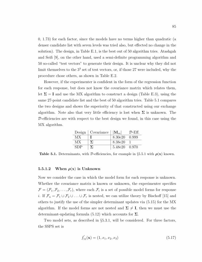
85
0, 1.73) for each factor, since the models have no terms higher than quadratic (a
denser candidate list with seven levels was tried also, but effected no change in the
solution). The design, in Table E.1, is the best out of 50 algorithm tries. Atashgah
and Seifi [9], on the other hand, used a semi-definite programming algorithm and
50 so-called “test vectors” to generate their design. It is unclear why they did not
limit themselves to the 33 set of test vectors, or, if those 27 were included, why the
procedure chose others, as shown in Table E.2.
However, if the experimenter is confident in the form of the regression function
for each response, but does not know the covariance matrix which relates them,
let Σ = I and use the MX algorithm to construct a design (Table E.3), using the
same 27-point candidate list and the best of 50 algorithm tries. Table 5.1 compares
the two designs and shows the superiority of that constructed using our exchange
algorithm. Note also that very little efficiency is lost when Σ is unknown. The
D-efficiencies are with respect to the best design we found, in this case using the
MX algorithm.
Design Covariance |Mm| D-Eff.MX I 8.30e20 0.999MX Σ 8.38e20 1SDP Σ 5.48e20 0.970
Table 5.1. Determinants, with D-efficiencies, for example in §5.5.1 with ρ(x) known.
5.5.1.2 When ρ(x) is Unknown
Now we consider the case in which the model form for each response is unknown.
Whether the covariance matrix is known or unknown, the experimenter specifies
F = (F1,F2, . . . ,Fr), where each Fi is a set of possible model forms for response
i. If Fu = F1 ∪ F2 ∪ . . . ∪ Fr is nested, we can utilize theory by Bischoff [15] and
others to justify the use of the simpler determinant updates via (5.15) for the MX
algorithm. If the model forms are not nested and Σ 6= I, then we must use the
determinant-updating formula (5.12) which accounts for Σ.
Two model sets, as described in §5.3.1, will be considered. For three factors,
the SSPS set is
f′
11(x) = (1, x1, x2, x3) (5.17)

86
f′
12(x) = (f11, x1x2, x1x3, x2x3) (5.18)
f′
13(x) = (f12, x21, x
22, x
23) (5.19)
so that F1,SSPS = f ′i (x)β1i, 1 ≤ i ≤ 3,x ∈ χ. Further, assume that F2,SSPS =
F1,SSPS so that both responses have the same set of possible models. Then,
Fu,SSPS = F1,SSPS ∪ F2,SSPS is nested and consequently we can use the simpler
algorithm.
The SPS set includes twelve models
f′
1+(x) = (1, x1) (5.20)
f′
2+(x) = (1, x2) (5.21)
f′
3+(x) = (1, x3) (5.22)
f′
4+(x) = (1, x1, x2, x3) (5.23)
f′
5+(x) = (f4+, x1x2) (5.24)
f′
6+(x) = (f4+, x1x3) (5.25)
f′
7+(x) = (f4+, x2x3) (5.26)
f′
8+(x) = (f4+, x1x2, x1x3, x2x3) (5.27)
f′
9+(x) = (f8+, x21) (5.28)
f′
10+(x) = (f8+, x22) (5.29)
f′
11+(x) = (f8+, x23) (5.30)
f′
12+(x) = (f8+, x21, x
22, x
23) (5.31)
so that F1,SPS = f ′i+(x)β1i+, 1 ≤ i ≤ 12,x ∈ X and F2,SPS = F1,SPS. This
set of models is not nested, so the SPS-model-robust design will depend upon Σ.
Using the MX algorithm of §5.4.1.2, we can calculate three model-robust designs:
SSPSMR (SSPS-model-robust, given in Table E.4); SPSMR-Σ (in the case that the
covariance matrix is known); and SPSMR-I (when the covariance is unknown), and
compare with the design optimal for the full quadratic alone (i.e. usual practice,
given in Table E.6). In this case SPSMR-Σ and SPSMR-I are the same (Table
E.5).
For a three-factor experiment, there are in total 63 possible models which obey

87
the oft-observed hierarchical principal (see [82, 13]), which says that higher-order
terms are included in the model only if appropriate lower-order terms appears.
Since there are two responses, this results in 632 = 3969 total possible hierarchical
models. To evaluate the model-robust designs described above, we have found the
optimal designs for each of these possible models individually (based upon only
10 algorithm tries due to computational constraints, and using a multiresponse
exchange algorithm in which only one exchange is made per iteration), allowing
us to calculate the D-efficiency of the model-robust designs with respect to each
of the 3969 models. We give relevant, comparative statistics in Table 5.2. For
these hierarchical models, the model-robust designs have higher D-efficiencies on
average, with less variability, than the design optimal for the full quadratic model.
Interestingly, while the design for the larger SPS set has less variability in its
efficiencies, its average is inferior to the design with respect to the smaller SSPS
set.
Design Mean StDev MinSSPSMR 0.940 0.037 0.829SPSMR-Σ/SPSMR-I 0.920 0.024 0.838Quadratic 0.915 0.056 0.740
Table 5.2. Comparison of model-robust designs for example in §5.5.1, in terms ofD-efficiencies with respect to all 3969 possible true models.
5.5.2 Two-factor, Two-response Experiment
We also consider a theoretical example in which there are two responses, two
factors and 12 runs, with both Σ and ρ(x) unknown. Since the covariance matrix
is unknown we assume Σ = I when constructing designs.
We can again use the algorithm of §5.4.1.2 to construct these model-robust
designs, one each with respect to the SSPS and SPS sets, using 50 algorithm tries
and a small 32 candidate list. In this case, the two designs turn out to be equivalent
(Table E.7). To evaluate the model-robustness of this design, we again consider
the set of all possible hierarchical models up through second order polynomials.
Since there are seven such models for each response, there are 72 = 49 models in
total.

88
We found the optimal designs for each of the 49 models (note that for conve-
nience we did not use the simplification of Equation (5.14) even when appropriate;
also, we again used an exchange algorithm similar to the one described in §5.4.1.2
except with only one swap made per iteration), for each of three assumed “true”
Σ:
Σ1 =
(1 0
0 1
), (5.32)
Σ2 =
(1 .8
.8 1
), (5.33)
Σ3 =
(9 1.5
1.5 1
). (5.34)
We also constructed the design optimal for the quadratic model alone (Table
E.8) and compared it with the model-robust design. Table 5.3 shows that the
model-robust design has a higher average and minimum D-efficiency, with smaller
standard deviation. For Σ1, we give histograms of these efficiencies for both de-
signs, as well.
SSPS/SPS Model-Robust Optimal for QuadraticMean StDev Min Mean StDev Min
Σ1 0.931 0.0468 0.825 0.893 0.0726 0.740Σ2 0.932 0.0482 0.825 0.894 0.0737 0.740Σ3 0.932 0.0481 0.825 0.894 0.0735 0.740
Table 5.3. Comparison of model-robust design and design optimal for full quadraticmodel, for each of three assumed true covariance matrices, as measured by the meanD-efficiency, standard deviation of the D-efficiency, and the minimum D-efficiency.
5.5.3 Mullet Meat Experiment
The final example, taken from Shah et al. [94] via Tseo et al. [101], was an ex-
periment in which washing minced mullet flesh was investigated. The controllable
factors were washing temperature (x1), washing time (x2), and washing ratio (x3)
and there were four responses: springiness (y1), thiobarbituric acid number (y2),
percent cooking loss (y3), and whiteness index (y4). The original experiment was
a central composite design with eight corner points, six axial points, and three

89
0.82 0.84 0.86 0.88 0.9 0.92 0.94 0.96 0.98 10
2
4
6
8
10
12
14
Figure 5.1. Histogram of D-efficiencies with respect to the 49 models and Σ1, for themodel-robust design.
center points (N = 17). Shah et al. [94] used an SUR model to fit the following
models:
y1 = 1.884634− 0.097383x1 − 0.103901x21 (5.35)
y2 = 22.648811 + 5.614804x1 − 0.341069x2 + 7.830449x21 + 2.681968x1x2 (5.36)
y3 = 18.956432 + 0.744422x1 − 0.207512x2 − 1.331086x3 + 3.222674x21
+ 1.392487x23 + 1.587398x1x2 + 1.804884x1x3 (5.37)
y4 = 51.910033 + 2.436441x1 − 3.428739x21 (5.38)
with estimated covariance matrix
Σ =
.0016525 −.0086836 −.0358445 −.0804776
−.0086836 7.5417141 −.5390002 2.4998582
−.0358445 −.5390002 4.5640517 4.8343599
−.0804776 2.4998582 4.8343599 14.2181839
. (5.39)
We first use the MX algorithm to produce, as a standard, the optimal design
using (5.35)-(5.38) and (5.39) as the truth (Table E.9). Then, we also construct

90
0.7 0.75 0.8 0.85 0.9 0.95 1 1.050
2
4
6
8
10
12
14
Figure 5.2. Histogram of D-efficiencies with respect to the 49 models and Σ1, for thedesign optimal for the quadratic model alone
two model-robust designs, one using the SSPS set (Table E.10) and the other using
the SPS set (Table E.11). We also include the design optimal for the quadratic
model alone in Table E.12. With respect to the particular “true” model forms and
covariance matrix, the design optimal for the quadratic model is 91.9% D-efficient,
while the model robust designs are only 89.2% and 88.2%, respectively. This is not
surprising because the fitted model forms include quadratic terms. If the “true”
models are modified such that three of the five quadratic terms are removed from
the model forms in (5.35)-(5.38) (x21 from y1 and y2 and x2
3 from y3), the SSPS-MR
and SPS-MR are 92.5% and 95.3% efficient, while the full quadratic is 91.1%.
5.6 Discussion
In this chapter we have generalized the matrix updating formulae of Fedorov [41]
to facilitate the development of an exchange algorithm to construct exact mul-
tiresponse designs. However, since neither the covariance matrix of the responses
or the model forms for each response is likely to be known at the design stage,
we extend the methodology and demonstrate that a model-robust approach can

91
be effective in constructing designs in the multiresponse context, compared to the
usual practice of ignoring the multiple responses and designing for the largest as-
sumed univariate model. Furthermore, our work confirms the general conclusion
of Chang [23] which found the effect of Σ on the optimal multiresponse design
to be minimal. Compared to the model response forms, the covariance matrix is
inconsequential.
When large problems are coupled with a large potential model set, computa-
tional requirements could become crippling, particularly if a higher granularity is
desired in the candidate list. For the small-to-moderate sized problems in this
chapter, model-robust designs can be computed in a reasonable amount of time.
However, to counteract debilitating computational demands for larger problems,
further work might include a coordinate exchange algorithm [77] for multiresponse
design, which would eliminate the need for a candidate list. For regular design
regions in particular, the extension should be straightforward.
Work has been done by Bingham and Chipman [13] which takes a more so-
phisticated view of selecting sets of a priori model forms. Instead of choosing
more or less ad hoc sets as we have in this work, these authors develop a prior
distribution of possible models based upon three axiomatic principles: Effect spar-
sity, effect hierarchy, and effect heredity. Their approach does not eliminate the
problem of exploding model size (in the end, they only handle a small subset of
the models with the largest prior probabilities), but it does represent a principled
approach that might be adapted to the current setting. However, we note that
1) this approach would further exaggerate the superiority of the model-robust de-
signs, because of the effect hierarchy assumption which favors lower-order effects
to higher-order ones; and 2) it would not be a straightforward application of their
methodology because we consider quadratic effects and require designs for which
these effects are estimable.

Chapter 6Maximin Model-Robust Designs for
Split Plot Experiments
6.1 Introduction
Split-plot experiments arise when certain factors are significantly harder and/or
more expensive to change (whole plot factors) than others (subplot factors). To
alleviate these difficulties, a two-step randomization scheme is employed. First, the
designer specifies the number of whole plots, and randomly assigns some combina-
tion of the whole plot factors to each. Then, within each whole plot, combinations
of subplot factor levels are randomly assigned to the subplots within each whole
plot. Thus, a split-plot design reduces the number of required independent resets
of the levels of the whole plot factors, compared to the completely randomized
design (CRD), and saves the experimenter time and/or money.
For instance, suppose an experiment is to be conducted to learn about factors
affecting the strength of a type of ceramic pipe. Two of the factors are concerned
with the temperature of different parts of a furnace, and are difficult to change
from run to run. The other two factors are the amount of binder and the grinding
speed, and are easy to change. A desirable design minimizes the number of changes
to the temperature factors–thus a split-plot design is appropriate. We return to
this example in §6.4.1.
For most of their history, split-plot experiments have been viewed as categorical
93
designs; that is, designs with qualitative factors. However, the recent split-plot
resurgence has viewed these as designed experiments with continuous factors and
this approach has spawned relatively recent work in the optimal design of split-plot
experiments. This helps to explain why there is not an asymptotic design theory
for split-plot experiments, though CRDs have a thorough asymptotic development.
Optimal design in this area, led by Goos and coauthors (e.g. [49, 50, 51,
59]), utilizes the D-optimality criterion to produce exact designs that estimate
model parameters as precisely as possible. As in the case of CRDs, these optimal
designs require the specification of a particular model form–an often unrealistic
assumption.
There is a paucity of extant research in model-robustness for split-plot experi-
ments. In this chapter, we provide a framework in which the model form assump-
tion can be relaxed and an exchange algorithm used to construct model-robust
split-plot designs. Instead of a single model, we allow the user to specify a set of
models; instead of directly using the D-criterion to construct the design, we use a
criterion which maximizes the minimum D-efficiency with respect to this set. A
generalization allows the experimenter to specify a level of interest in each model,
giving the experimenter recourse if certain models are preferred over others, and
flexibility to inject prior belief into the design process. We find also, corroborat-
ing previous work, that the ratio of variance components has little impact on the
optimal design.
6.2 The Split-Plot Model and Design
Here, we follow the notation of Goos and Vandebroek [49]. A split-plot experi-
ment consists of two disparate groups of factors: the nw difficult to change whole
plot variables, denoted z = (z1, z2, . . . , znw), and the remaining ns easy to change
subplot factors, denoted x = (x1, x2, . . . , xns). Whole plot factor level combina-
tions are randomly assigned to the whole plots, and then within each whole plot
factor level combinations of x are randomly assigned. We can represent an exact

94
split-plot design as
ξnb =
((z1,x11) (z1,x12) . . . (z1,x1u1) (z2,x21) . . . (zb,xbub
)
n11 n12 . . . n1u1 n21 . . . nbub
)(6.1)
where n is the total number of runs, b is the number of whole plots, ui is the
number of distinct points in the ith whole plot, and nik is the number of runs for
the kth distinct point in the ith whole plot.
The regression model for the jth observation within the ith whole plot is
yij = f′(zi,xij)τ + δi + εij (6.2)
where f is the model expansion in terms of the whole plot and subplot factors, τ
is a p-vector of model parameters, δi is the whole plot error term, and εij is the
subplot error term. The parameter vector includes pw parameters for whole plot
factors only, ps parameters for subplot factors only, and pws parameters for whole
plot-by-subplot interactions. We can write the model in matrix notation as
Y = Xτ + δ + ε (6.3)
Both δi and εij are assumed to be normally distributed with mean 0 and vari-
ances σ2δ and σ2
ε , respectively. Each observation yij has two variance components,
one contributed by the whole plot, σ2δ , and one contributed by the subplot, σ2
ε .
Thus, V ar(yij) = σ2δ + σ2
ε . However, within whole plot i, observations are corre-
lated because the whole plot is fixed. This is represented by Cov(yij, yij′) = σ2δ ,
where j 6= j′. Thus, the variance-covariance matrix for whole plot i is
Wi = σ2ε Isi
+ σ2δ1si
1′
si
= σ2ε (Isi
+ η1si1′
si)
where η = σ2δ/σ
2ε , si is the number of runs in whole plot i, Isi
is the identity
matrix, and 1siis an si-vector of ones. Since the whole plots are assumed to be

95
independent of one another, the covariance matrix for (6.3) is block diagonal:
W =
W1 0 . . . 0
0 W2 . . . 0...
.... . .
...
0 0 . . . Wb
To estimate the parameters of this model, we use Generalized Least Squares
(GLS), which give τ =(X′W−1X
)−1X′R−1Y so that V ar(τ ) =
(X′W−1X
)−1.
The information matrix, then, is
Msp = X′W−1X.
This expression for the information matrix can be simplified [49]; see Appendix
F.1 for details. First, W−1i can be written as
W−1i =
1
σ2ε
(Isi− d
1 + sid1si
1′
si
)which leads to a convenient, updatable form of the information matrix:
Msp =w∑i=1
X′
iW−1i Xi
=1
σ2ε
(w∑i=1
si∑j=1
f(zi,xij)f′(zi,xij)−
w∑i=1
d
1 + sid(X
′
i1si)(X
′
i1si)′
).
In this chapter, we are primarily interested in D-optimality, which is given by
|Msp| =∣∣∣X′
W−1X∣∣∣ . (6.4)
We also give the prediction variance for design ξ and point (zi,xij), because our
algorithm uses it to construct an initial design:
Vsp(zi,xij, ξ) = f′(zi,xij)M
−1sp (ξ)f(zi,xij). (6.5)

96
6.3 Model-Robust, Maximin Split-Plot Design
Algorithm
In this section, we first review the basic idea of the exchange algorithm for D-
optimal split-plot designs, given by Goos and Vandebroek [50]. We then give a
generalization of the algorithm which is robust to a set of user-specified models,
achieving this robustness by seeking the design which maximizes the minimum
D-efficiency with respect to the model set.
6.3.1 D-Optimal Split-Plot Exchange Algorithm
The algorithm upon which ours is based [50] requires the specification of the num-
ber of whole plots as well as the number of subplots per whole plot. The same
authors [51] also give an algorithm for which these requirements are relaxed. How-
ever, when split-plot experiments are called for, it is most often because certain
factors are difficult or expensive to change. Thus, at the very least an algorithm
is desired for which the number of whole plots can be constrained, and for our
purposes we will consider only the case in which the number and size of the whole
plots are explicitly specified.
Thus, the D-optimal split-plot algorithm requires the construction of a candi-
date list, the number and size of the whole plots, the ratio of variance components,
η = σ2δ/σ
2ε , and a given, assumed model form. The algorithm first randomly spec-
ifies an initial design, and then iteratively improves upon the design using three
exchange mechanisms: 1) Consider swaps of current design points with candidate
points having the same whole plot factor settings; 2) Consider swaps of current
design points with other design points having the same whole plot factor settings;
and 3) Consider swaps of current whole plot factor settings with other possible
whole plot factor settings. For each mechanism in turn, all possible exchanges
are considered for each appropriate design point (or whole plot). The algorithm
iterates until convergence. Since this is not a concave optimization problem, the
algorithm is not guaranteed to converge to the globally optimal solution. Conse-
quently, numerous algorithm tries, each with a randomly generated initial design,
are used to overcome possibly local optima (we use 50 tries, and Goos and Vande-

97
broek [50] give evidence that this is adequate to produce an optimal design with
high probability). The model-robust algorithm developed below is similar to this
procedure in structure and approach.
Many updates of the determinant of the split-plot information matrix are re-
quired as exchanges are considered. Arnouts and Goos [5] developed updating
formulae that speed the computation of these updates. We reproduce them in
Appendix F.2, and refer to them in our algorithm as they are used.
6.3.2 Maximin Split-Plot Exchange Algorithm
In this section we describe a model-robust procedure for the split-plot optimal
design problem which parallels that in Chapter 4 for the completely randomized
setting. This is based upon F , a user-specified set of r models. Our goal is to
find a design that is maximin optimal with respect to a generalized measure of
D-efficiency, Gf (ξnb), defined as
Gf (ξnb) =Df (ξnb)
vf(6.6)
where vf represents the model interest (weight) element for model f and Df (ξnb)
is the D-efficiency for a design ξnb with respect to model f , calculated as
Df (ξnb) =
(|Msp,f (ξnb)||Msp,f (ξ∗nb)|
)1/p
(6.7)
where ξ∗nb is the optimal design for model f . The model interest vector is v =
(v1, . . . , vr) ∈ (0, 1] and represents the experimenter’s level of interest in each of
the r specified models. By convention, we scale this vector so that the a priori
most likely model(s) has (have) a model interest level of 1. (Note that the user
could renormalize these model interest weights as prior probabilities.) The algo-
rithm gives a lower priority to models with smaller interest levels and in fact gives
precedence to each model commensurate with its model interest level. This hier-
archy is sometimes reflected in the efficiencies of the design with respect to the
models in F (i.e. if F = (f1, f2) and v = (1, .8), the resulting design may have a
D-efficiency with respect to the second model form that is about 80% that of the

98
first). Due to the discrete nature of the exact split-plot design problem, as well as
complications inherent in model sets with more than two elements (see Chapter
4), the efficiency precedence may be obscured or nonexistent, as demonstrated in
our examples.
This model-robust procedure is computationally more demanding than the orig-
inal split-plot exchange algorithm. First, there are r models to consider instead
of just one. Secondly, it requires that the optimal design for each of the models
individually be found. There are fewer commercially available optimal design al-
gorithms for split-plot experiments than for CRDs, though they do exist (e.g. SAS
JMP). However, if the model-robust algorithm is implemented the optimal design
split-plot algorithm is a special case when F consists of just a single model, and
thus could be used to furnish the individually optimal designs.
To describe our algorithm, we adopt the same basic structure (though different
notation) as Goos and Vandebroek [50]: There is assumed to be c candidate points,
the set of which is denoted by C. Similarly, there are b whole plots and the set
of them is B, and the ki design points in the ith whole plot for a design ξnb are
denoted by Hi. Thus, the total number of design points is n =∑b
i=1 ki. The whole
plot factor level combinations for the ith whole plot is given by zi, and the set of
candidate points with the same whole plot factor combinations as the ith whole
plot is given by Ci. The generalized D-efficiency for model f is Gf , as in (6.6).
The best minimum generalized efficiency found at any given point in the algorithm
is represented as G∗fmin. Also, we let the set of possible whole plot factor levels be
P . The number of algorithm tries is given by t and the current try is tc. See §6.4.1
for an illustration of this notation.
For the algorithm, we must specify 1) a candidate list, C; 2) the number of
whole plots, b; 3) the size of each whole plot, k1, k2, . . . , kb; 4) the ratio of variance
components, η; 5) the set of possible model forms, F ; 6) a model interest vector,
v, specifying the relative preference for each model (if no preferences, enter vf = 1
for all f ∈ F ; and 7) for each model f ∈ F ,∣∣Msp,f (ξ
∗f )∣∣, where ξ∗nb,f is the optimal
design for model f alone. One consequence of our set of models approach is that the
number of whole plots, b, must be greater than pw,fmax , the number of parameters
with only whole plot terms, for the largest model. The algorithm is as follows:
1. Set tc = 1.

99
2. Determine pw,f , the number of coefficients for whole plot factors only, for all
f ∈ F .
3. Determine ps,f , the number of coefficients for subplot factors only, for all
f ∈ F .
4. Set Msp,f = ωI (where ω is a small constant set at 0.01) for all f ∈ F ; set
Hi = ∅.
5. Construct initial design
(a) Randomly assign pw,fmax unique whole-plot factor settings to pw,fmax
whole plots, where fmax is the model with the most parameters (to
ensure estimability of whole plot coefficients for largest model).
(b) Randomly assign b− pw,fmax levels of the whole-plot factors to the rest
of the whole plots.
(c) Randomly choose u (1 ≤ u ≤ pfmax), where pfmax is the number of
parameters for model fmax.
(d) Do u times (this step gives initial design a measure of randomness):
i. Randomly select i ∈ B (select a whole plot at random)
ii. Randomly select j ∈ Ci (select a candidate point with the ith setting
of whole plot, at random)
iii. If #Hi < ki, then Hi = Hi ∪ j; otherwise, go back to step i.
iv. Update M−1sp,f for all f ∈ F via (F.1).
(e) Do n − u times (this step attempts to give initial design a measure of
quality with respect to all models f ∈ F):
i. Randomly select f ∈ F .
ii. Set l = 1.
iii. For model f , determine j ∈ C with the lth biggest prediction vari-
ance via (6.5).
iv. Find i, where i ∈ B, j ∈ Ci, and #Hi < ki (find a nonfull whole
plot into which j can be inserted). If no such i exists, set l = l + 1
and return to step iii.

100
v. Hi = Hi ∪ j.
vi. Update M−1sp,f for all f ∈ F via (F.1).
6. Compute M−1sp,f for all f ∈ F and Gfmin
(the smallest generalized efficiency).
If Gfmin= 0, go back to step 4. Otherwise, continue.
7. Set ν = 0.
8. Evaluate design point exchanges (swapping design points with candidate
points, where whole plot factors settings are the same):
(a) Set γ = Gfmin= minf∈F Gf .
(b) ∀i ∈ B, ∀j ∈ Hi, ∀k ∈ Ci, j 6= k:
i. Determine the effect δijk,fmin= |Mi
jk,sp,fmin|/|Msp,fmin
| of exchang-
ing, in the ith whole plot, points j and k, using (F.4).
ii. If δijk,fmin> 1, calculate δijk,f = |Mi
jk,sp,fmin|/|Msp,fmin
| for all f 6=fmin and update |Msp,f | for all f ∈ F via (F.4). Then, compute
Gijk,f for all f ∈ F .
iii. If minf∈F Gijk,f > γ, then γ = minf∈F G
ijk,f and store i, j, and k.
9. If γ > Gfmin+ ε, then go to step 10; otherwise, go to step 11.
10. Perform the best exchange:
(a) Hi = Hi \ j ∪ k.
(b) Update M−1sp,f and |Msp,f | for all f ∈ F via (F.5) and (F.4), respectively.
(c) Set ν = 1.
11. Evaluate interchanges of points within whole plots with the same factor lev-
els:
(a) Set γ = Gfmin= minf∈F Gf .
(b) ∀i, j ∈ B, i < j, zi = zj, ∀k ∈ Hi, ∀l ∈ Hj, k 6= l:
i. Determine the effect δjlik,fmin= |Mjl
ik,sp,fmin|/|Msp,fmin
| of moving k
to whole plot j (from whole plot i) and l to whole plot i (from whole
plot j), via (F.7).

101
ii. If δjlij,fmin> 1, calculate δjlik,f = |Mjl
ik,sp,fmin|/|Msp,fmin
| for all f 6=fmin and update |Msp,f | for all f ∈ F via (F.7). Then, compute
Gjlik,f for all f ∈ F .
iii. If minf∈F Gjlik,f > γ, then γ = minf∈F G
jlik,f and store i, j, k, and l.
12. If γ > Gfmin+ ε, go to step 13; otherwise, go to step 14.
13. Perform the best interchange:
(a) Hi = Hi \ k ∪ l.
(b) Hj = Hj \ l ∪ k.
(c) Recalculate M−1sp,f and update |Msp,f | via (F.7).
(d) Set η = 1.
14. Evaluate exchanges of whole-plot factor settings:
(a) Set γ = Gfmin= minf∈F Gf .
(b) ∀i ∈ B, ∀j ∈ P , zi 6= zj:
i. Determine the effect δij,fmin= |Mij,sp,fmin
|/|Msp,fmin| of exchanging
zi by zj in the ith whole plot, via (F.10).
ii. If δij,fmin> 1, calculate δij,f = |Mij,sp,fmin
|/|Msp,fmin| for all f 6=
fmin and update |Msp,f | for all f ∈ F via (F.10). Then, compute
Gij,f for all f ∈ F .
iii. If minf∈F Gij,f > γ, then γ = minf∈F Gij,f and store i and j.
15. If γ > Gfmin+ ε, go to step 16; otherwise, go to step 17.
16. Perform best exchange:
(a) Update Hi and Ci.
(b) Update M−1sp,f and |Msp,f | for all f ∈ F via (F.11) and (F.10), respec-
tively.
(c) Set η = 1.
17. If η = 1, go to step 7.

102
18. If Gfmin= minf∈F Gf > G∗fmin
, then G∗fmin= Gfmin
; also, update the design
ξnb.
19. If tc < t, then tc = tc + 1, and go back to step 4; otherwise, STOP.
Notes: 1) This algorithm, including Step 5 which generates the initial design,
generalizes Goos and Vandebroek [50] but follows its basic outline. 2) In 13(c),
we recalculate M−1 by directly taking its inverse, because of numerical issues
associated with the updated formula in (F.8). This should have a minimal effect
on the speed of the algorithm because it occurs only once per iteration. 3) In steps
9, 12, and 15, we have changed the original algorithm of Goos and Vandebroek [50]
slightly by requiring that, for any considered exchange/interchange, the increase
in the minimum efficiency is greater than ε = 0.0001 (instead of 0, as it was
originally), to encourage algorithmic stability. 4) Note that the ε here is not a
convergence parameter as in the previous chapters. For a particular algorithm try,
tc, the procedure terminates when an iteration results in no exchanges.
6.4 Examples
In this section we illustrate our model-robust procedure using two examples from
the literature. The first involves two whole plot factors and two subplot factors.
The second includes two process (whole plot) factors and three mixture (subplot)
factors. In what follows, we reference and discuss a large number of designs. In the
interest of space, they can be found in the supplementary material accompanying
this article. All designs referred to in the following examples are given in Appendix
H. Matlabr (Version 7.8) code can be found at http://www.stat.psu.edu/~jlr/
pub/Smucker/.
6.4.1 Strength of Ceramic Pipe Experiment
In a reprise of the example at the outset, the first example is taken from Vining
et al. [103] and concerns an experiment on the strength of ceramic pipe. To
illustrate and clarify the notation for the algorithm in the previous section, we will
include that notation in the description of this example. There were four factors,

103
two hard-to-change (zone 1 temperature of furnace, z1; zone 2 temperature of
furnace, z2) and two easy-to-change (amount of binder, x1; grinding speed, x2).
The experiment used b = 12 whole plots each of size 4 (ki = 4 for i = 1, . . . , 12 so
that n =∑12
i=1 ki = 48). A given design for this experiment is denoted by ξnb and
the part of the design associated with the ith whole plot is Hi.
After running the experiment, it was found that η = σ2δ/σ
2ε = .52828/.09348 =
5.65. The model to be fit was full quadratic in all factors:
f′(z,x) = (1, z1, z2, z1z2, z
21 , z
22 , x1, x2, x1x2, z1x1, z1x2, z2x1, z2x2, x
21, x
22) (6.8)
with X = z = (z1, z2),x = (x1, x2) : −1 ≤ z,x ≤ 1.Vining et al. [103] used a face-centered central composite design (CCD) mod-
ified to accommodate the split-plot structure. Another design approach would
be to use the D-optimal exchange algorithm of Goos and Vandebroek [50] (or,
alternatively, the candidate list-free exchange algorithm of, [59]) assuming (6.8)
to be the true model. In retrospect, this model seemed to be a good approxi-
mation of the true model [103], but if the experimenter were not confident about
the form of the model a priori, it would be advantageous to choose a set of mod-
els and construct a design robust for all of them. For instance, we might choose
F1 = f ′i (z,x)τi, 1 ≤ i ≤ 3; z,x ∈ X with
f′
1(z,x) = (1, z1, z2, x1, x2) (6.9)
f′
2(z,x) = (f′
1, z1z2, x1x2, z1x1, z1x2, z2x1, z2x2) (6.10)
f′
3(z,x) = (f′
2, z21 , z
22 , x
21, x
22). (6.11)
A weakness of optimal design—addressed for exact designs in an ad-hoc way
in the split-plot case by Goos and Donev [47] and in a more systematic way in
the CRD case by, for instance, DuMouchel and Jones [37] and Goos et al. [48]—is
that it devotes all of the available experimental resources to increase the efficiency
of the design and none to allow lack-of-fit testing. To overcome this shortcoming,
while remaining in the optimal design paradigm and thus enjoying a great deal of
efficiency, a strategy would be to construct a design somewhat less efficient with
respect to models considered likely, while affording the experimenter estimability

104
for a larger model. This approach can serve as a hedge against a larger-than-
expected model, though it does not necessarily allow traditional lack-of-fit testing.
To illustrate, we take F2 = F1, f′4 with
f4 = (f3,x1x2x3, x1x2x4, x1x3x4, x2x3x4, (6.12)
x21x2, x
21x3, x
21x4, x
22x1, x
22x3, x
22x4, x
23x1, x
23x2, x
23x4, x
24x1, x
24x2, x
24x3,
x31, x
32, x
33, x
34),
the full cubic model.
In Table 6.1, we consider seven designs in all, evaluating them by calculating
their D-efficiencies with respect to each of the possible models we have discussed.
The first four are based on the methodology developed in this work, and the last
three are included for comparative purposes. The maximin designs, as well as
the optimal designs for models (6.11) and (6.12), have been calculated under the
assumption that the variance components are the same (i.e. no prior knowledge
of η) and the best of t = 50 algorithm tries taken, each starting with a randomly
chosen design, using a 54 candidate list–all combinations of (−1,−0.5, 0, 0.5, 1) for
each of the four factors. Thus, c = 54 = 625 and C is the set of these points,
while Ci is the portion of these points whose whole plot factor combinations match
that of the ith whole plot. This also implies that P , the possible factor level
combinations of the two whole plot factors, consists of 52 points (all combinations
of (−1,−0.5, 0, 0.5, 1)).
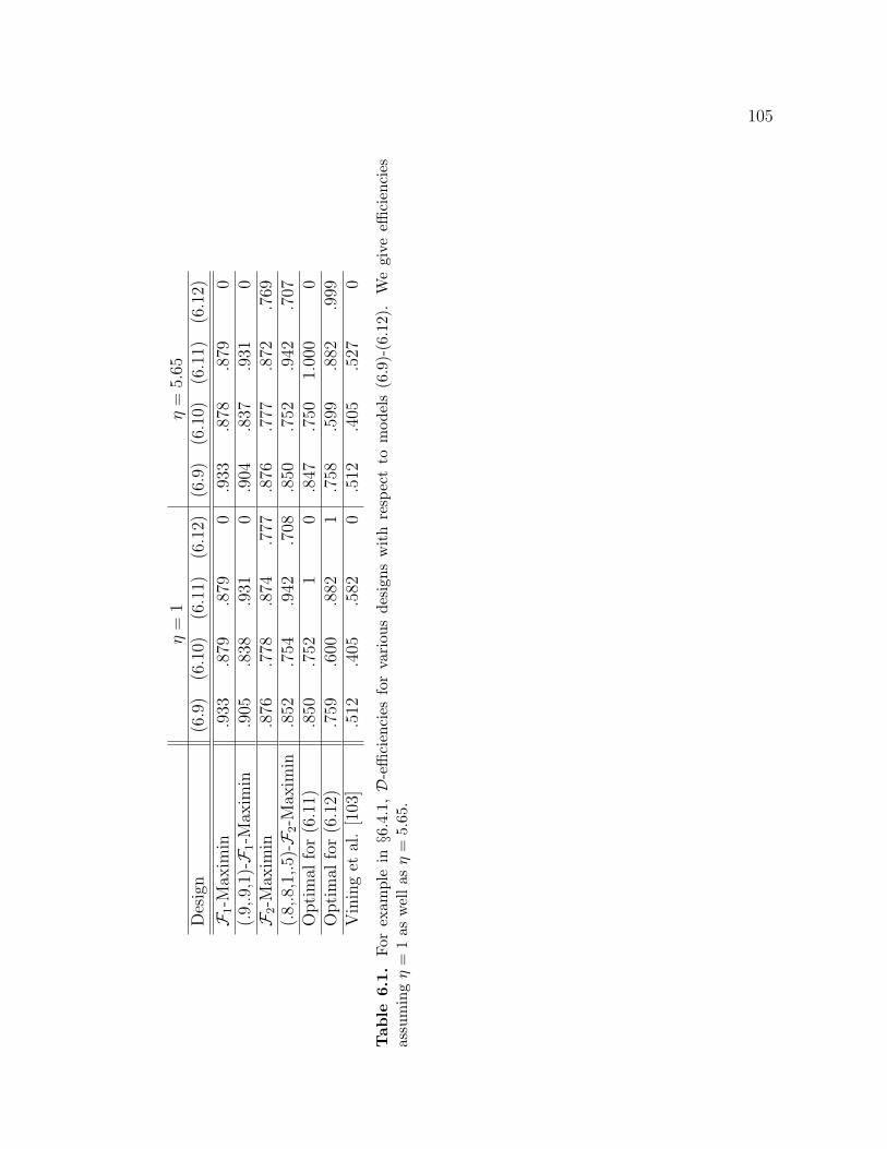
105
η=
1η
=5.
65D
esig
n(6
.9)
(6.1
0)(6
.11)
(6.1
2)(6
.9)
(6.1
0)(6
.11)
(6.1
2)
F1-M
axim
in.9
33.8
79.8
790
.933
.878
.879
0(.
9,.9
,1)-F
1-M
axim
in.9
05.8
38.9
310
.904
.837
.931
0F
2-M
axim
in.8
76.7
78.8
74.7
77.8
76.7
77.8
72.7
69(.
8,.8
,1,.5)
-F2-M
axim
in.8
52.7
54.9
42.7
08.8
50.7
52.9
42.7
07O
pti
mal
for
(6.1
1).8
50.7
521
0.8
47.7
501.
000
0O
pti
mal
for
(6.1
2).7
59.6
00.8
821
.758
.599
.882
.999
Vin
ing
etal
.[1
03]
.512
.405
.582
0.5
12.4
05.5
270
Tab
le6.
1.Fo
rex
ampl
ein§6
.4.1
,D
-effi
cien
cies
for
vari
ous
desi
gns
wit
hre
spec
tto
mod
els
(6.9
)-(6
.12)
.W
egi
veeffi
cien
cies
assu
min
gη
=1
asw
ell
asη
=5.
65.

106
In Table 6.1, we calculate the efficiencies both under the assumption that η = 1
and η = 5.65 (estimated by Vining et al. [103]). It can be seen that η has almost
no effect on the efficiencies of the designs. The maximin design with respect to
F1 is relatively efficient for the three models, but cannot estimate the larger cubic
model, (6.12). The (.9,.9,1)-F1-maximin design is appropriate if more emphasis
is desired for the quadratic model, (6.11), than the smaller ones. In comparison
to the design optimal for the quadratic model alone, this design gives up some
precision for the quadratic model but is more efficient for the two smaller models.
However, if some protection is desired for a lurking, higher-order model we
expand to the set F2. The F2-maximin design shows, unsurprisingly, that adding
the full cubic model dampens the ability to estimate the other models. However, if
we take v = (.8, .8, 1, .5) and compare the resulting maximin design to the optimal
design for (6.11), this design estimates the smaller models as well, gives up just 6%
in efficiency for the quadratic model and simultaneously allows for 71%-efficient
estimation of the full cubic model.
In terms of D-efficiency, the design proposed by Vining et al. [103] (a CCD in
the whole plot factors with various subplot designs at each whole plot) is not com-
petitive, but this does not necessarily preclude it from the consideration of the ex-
perimenter. It has other qualities—for instance, it allows for a model-independent
estimate of the variance components and a replication-based lack-of-fit test—that
recommend it to an experimenter that wishes to remain within the structure of
classic designs (i.e. CCDs).
6.4.2 Vinyl-Thickness Experiment
We next consider an example given in Cornell [29] and used later by Kowalski et
al. [68] and Goos and Donev [47]. This experiment measured the thickness of
manufactured vinyl for automobile seat covers and included two process factors
(extrusion rate, z1, and drying temperature, z2) and three mixture factors (plas-
ticizers, x1, x2, and x3). Complete randomization was unwieldy, so the process
variables were treated as whole plot factors, and the mixture variables as subplot
factors. Though the original design was run in eight whole plots each of size six,
Kowalski et al. [68] and Goos and Donev [47] used only 28 total runs, with 7 whole

107
plots each of size 4. We will adopt this approach as well.
The model used by Kowalski et al. [68] and Goos and Donev [47] was as in
(6.2) with z,x ∈ X where
f′(z,x) = (x1, x2, x3, x1x2, x1x3, x2x3, z1x1, z2x1, z1x2, z2x2, z1x3, z2x3, z1z2)
(6.13)
and
X =
z = (z1, z2),x = (x1, x2, x3) : −1 ≤ z,x ≤ 1;
3∑i=1
xi = 1
.
Since this experiment involved both mixture and process variables, the model
is a combination of an interaction model for the process factors and a second-order
Sheffe polynomial model for the mixture factors (see [68]). The designs of [68]
and [47] assumed the model in (6.13) but in the analysis done by Kowalski et al.
[68] it was concluded that few of the terms were significant and thus the assumed
model was overspecified. This was not, of course, known before the experiment was
conducted, and illustrates why it might be desirable to use a design that accounts
for more than just a single, assumed model.
To demonstrate the flexibility of our algorithm, we will consider two experi-
mental scenarios. The first assumes that there is a high degree of confidence that
the true model includes some combination of terms in the original fitted model. In
this case, it would make sense to choose F1 = f ′1i(z,x)τ1i, 1 ≤ i ≤ 6; z,x ∈ Xwith
f′
11(z,x) = (x1, x2, x3) (6.14)
f′
12(z,x) = (f′
11, x1x2, x1x3, x2x3) (6.15)
f′
13(z,x) = (f′
11, z1x1, z2x1, z1x2, z2x2, z1x3, z2x3) (6.16)
f′
14(z,x) = (f′
13, z1z2) (6.17)
f′
15(z,x) = (f′
12, z1x1, z2x1, z1x2, z2x2, z1x3, z2x3) (6.18)
f′
16(z,x) = (f′
15, z1z2) (6.19)
as a set of possible models, the largest of which is equivalent to (6.13). These
designs have no estimation abilities for models with higher order terms, so if the
experimenter wishes to guard against this possibility, consider augmenting F1 with

108
several such models: F2 = (F1, f′2i(z,x)τ2i, 1 ≤ i ≤ 6; z,x ∈ X where
f′
21(z,x) = (f′
12, x1x2x3) (6.20)
f′
22(z,x) = (f′
14, z21 , z
22) (6.21)
f′
23(z,x) = (f′
15, x1x2x3) (6.22)
f′
24(z,x) = (f′
15, z1z2, x1x2x3) (6.23)
f′
25(z,x) = (f′
16, z21 , z
22) (6.24)
f′
26(z,x) = (f′
24, z21 , z
22) (6.25)
In all the maximin (and individually optimal) designs for this example, we
use 50 algorithm tries with a 90-element candidate list (a 32 list for the whole
plot variables crossed with a 10-element set of mixture points: (1, 0, 0), (0, 1, 0),
(0, 0, 1), (1/2, 1/2, 0), (1/2, 0, 1/2), (0, 1/2, 1/2), (1/3, 1/3, 1/3), (2/3, 1/6, 1/6),
(1/6, 2/3, 1/6), and (1/6, 1/6, 2/3)). We have assumed η = 1 throughout.
In Table 6.2 we show the efficiencies of the F1-maximin and (.7, .9, 1, 1, 1, 1)-
F1-maximin designs with respect to models (6.14)-(6.25). We also give a design
which explicitly accounts for all models in F2, the (1, 1, 1, 1, 1, 1, .5, .5, .5, .5, .5, .5)-
F2-maximin design. Compared to the design optimal for the original assumed
model,(6.13), the F1-Maximin design successfully raises the lowest of the efficien-
cies for the models in F1. The second design represents the situation in which the
experimenter cares most about estimating models (6.16)-(6.19).
The third design gives up estimability for models (6.14)-(6.19) but allows the
estimability of the models (6.20)-(6.25). These latter models have model interest
vector elements of 0.5, so we might expect the efficiencies of these models to be
lower, say about 50% of the efficiencies for those models with model interest vec-
tor elements of 1. This is not the case, however, and we conjecture that in the
asymptotic case (i.e. when both the number and size of the whole plots tends to
infinity), and with a larger candidate list, the efficiencies would be more suggestive
of the differences in the model interest vector. Even with model interest vector
elements for the last six models of 0.3 or 0.15 instead of 0.5, designs with similar
efficiencies resulted. See the last section for more discussion of this point.
When the experimenter believes that a model more complex than (6.13) is some-

109
what likely, designs giving more weight to the higher order models in F2 are appro-
priate. In Table 6.3 we include the F2-maximin design, as well as one in which the
larger models are downweighted slightly, with v = (1, 1, 1, 1, 1, 1, .9, .9, .9, .9, .9, .9).
To demonstrate that quality designs can be obtained using a well-chosen subset of
F2, we include two designs based upon
F3 = f ′11(z,x)τ11, f′
16(z,x)τ16, f′
26(z,x)τ26, (6.26)
as well. As a benchmark, we compare these designs with the design optimal for
(6.25).
The design optimal for (6.25) does not estimate models (6.22) or (6.23) pre-
cisely. All of the maximin designs do much better for these models, and it under-
scores the general point that the maximin designs allow control of the worst-case
much better than using a design optimal for a single model. Furthermore, the
(.7, 1, .9)-F3-Maximin design dominates the individually optimal design for 10 of
12 models (the F2-Maximin design is better for 9 of 12, whereas the other two
designs only 6 of 12).

110
Des
ign
(6.1
4)
(6.1
5)
(6.1
6)
(6.1
7)
(6.1
8)
(6.1
9)
(6.2
0)
(6.2
1)
(6.2
2)
(6.2
3)
(6.2
4)
(6.2
5)
F1-M
axim
in.8
71
.896
.872
.885
.973
.975
00
00
00
(.7,.
9,1,1,1,1
)-F
1-M
axim
in.9
07
.814
.915
.923
.967
.969
00
00
.012
0(1,1,1,1,1,1,.
5,.
5,.
5,.
5,.
5,.
5)-F
2-M
axim
in.8
88
.823
.823
.812
.904
.888
.626
.923
.806
.799
.956
.854
Op
tim
al
for
(6.1
3)
.831
.958
.831
.847
11
00
00
00
Kow
als
ki
etal.
[68]
.430
.555
.354
.375
.475
.481
.593
0.5
20
.511
00
Tab
le6.
2.Fo
rex
ampl
ein§6
.4.2
,des
igns
focu
sed
onsm
alle
rm
odel
s,w
ithD
-effi
cien
cies
for
mod
els
(6.1
4)-(
6.25
),as
sum
ingη
=1
Des
ign
(6.1
4)
(6.1
5)
(6.1
6)
(6.1
7)
(6.1
8)
(6.1
9)
(6.2
0)
(6.2
1)
(6.2
2)
(6.2
3)
(6.2
4)
(6.2
5)
F2-M
axim
in.8
66
.874
.801
.792
.919
.901
.798
.905
.908
.894
.969
.942
(1,1,1,1,1,1,.
9,.
9,.
9,.
9,.
9,.
9)-F
2-M
axim
in.8
82
.833
.817
.807
.899
.882
.763
.918
.887
.873
.952
.926
F3-M
axim
in.8
87
.834
.815
.805
.905
.889
.771
.916
.895
.880
.956
.932
(.7,1,.
9)-F
3-M
axim
in.8
22
.948
.767
.762
.937
.918
.859
.875
.928
.910
.986
.958
Op
tim
al
for
(6.2
5)
.763
.904
.662
.658
.838
.819
.954
.854
.906
.882
.960
1
Tab
le6.
3.Fo
rex
ampl
e§6
.4.2
,de
sign
sfo
cusi
ngon
both
smal
lan
dla
rge
mod
els,
wit
hD
-effi
cien
cies
for
mod
els
(6.1
4)-(
6.25
),as
sum
ingη
=1

111
6.5 Discussion
In this chapter we have presented a generalization of the split-plot exchange al-
gorithm of Goos and Vandebroek [50] which relaxes the model form assumption
inherent in optimal design by designing with respect to a set of specified possible
models. Our algorithm tries to choose the design which maximizes the smallest
D-efficiency with respect to the specified models, robustifying the experiment to
the models in the set. This approach requires that the optimal designs for each of
the individual models in the set be found, but once these are in hand the experi-
menter is afforded much more flexibility because they can specify a model interest
vector that quantifies the relative interest in each model.
In Chapter 4, we have used this criterion to construct model-robust designs
in the CRD case. There, the efficiencies more faithfully reflect the model inter-
est vector than do the maximin designs in this chapter. In fact, several results
were proven in the CRD case regarding the balance of these designs in terms of
their D-efficiencies for a given set of models (e.g. for a given set of models, the
maximin design will include at least two whose generalized D-efficiencies are the
same). However, these were results assuming infinite run sizes, drawing on clas-
sical asymptotic design theory. The same basic asymptotic development does not
exist, to our knowledge, for restricted randomization designs; further research is
necessary. We conjecture that these “balance” type results have split-plot analogs.
However, even if our conjecture is correct, for finite run sizes such balance may
not be evident, due to the typically small number and size of the whole plots
in these experiments and the lack of a dense enough candidate list. This latter
difficulty could be mitigated somewhat by generalizing the algorithm of Jones and
Goos [59], which requires no candidate list. The original algorithm was limited in
that it could not work for constrained design spaces, but recent work reports that
it is possible [86, 59].
Within the “set of models” framework, other criteria could have been used.
For instance, several authors [71, 27, 54, 95] use something akin to∏m
i=1 |Mi(ξn)|as a model-robust criterion. This obviates the need for first obtaining the optimal
designs for each of the individual models. The downside is the lack of flexibility
for the experimenter in terms of the efficiencies with respect to each model: If

112
the design favors one model over another (say, by endowing the former with an
efficiency very close to 1 and the latter with a much lower efficiency), the only
recourse might be to try weighting the criterion:∏m
i=1 |Mi(ξn)|ai . However, in the
CRD case, this proved ineffective. Overall, with the ever-increasing computational
power at hand, we feel that the extra work is worth the additional flexibility
afforded by the maximin criterion.
Extensive simulations have been done (e.g. [49]) demonstrating that the ratio
of variance components, η, has a minimal effect on the optimal designs. Our work
here confirms that, and is shown in particular in Table 6.1. The second example,
although we do not show the efficiencies under the estimated η, gives similar re-
sults. In short, very little information is lost by a lack of a priori knowledge of
η, particularly when compared to the precision lost when an incorrect model is
assumed. Though we do not understand precisely why this is the case, it comports
with other research (Chapter 5, [23]) in which the correlated, multiple responses
seem to have little effect on experimental design.

Chapter 7Contributions and Future Work
In this dissertation, a practical model-robust framework for exact experimental
design is presented and implemented via generalizations of an existing exchange al-
gorithm. We consider several experimental situations, including two model-robust
procedures for the univariate and completely randomized design scenario, as well
as model-robust procedures to account for multiple responses and split-plot exper-
iments. In this chapter, we review the contributions of this work, and give some
possible future research directions.
7.1 Contributions
7.1.1 Single Response Model-Robust Experimental Design
In Chapter 3 a generalization of the modified Fedorov exchange algorithm has been
developed to construct exact designs which are robust to a set of user-specified po-
tential model forms. The product of the determinants of the information matrices
for each of the possible models is used as a criterion and a connection is made be-
tween these model-robust designs and the D-optimal multiresponse design whose
responses have the same model forms as the potential models. Specifically, if the
model forms are nested the model-robust design is the same as the optimal design
for this associated multiresponse model.
The designs produced by this model-robust procedure compare favorably to
the designs produced by competing procedures in the literature. The MRMF

114
designs are competitive with and simpler to implement than the Genetic Algorithm
approach of Heredia-Langner et al. [54]. Compared to the Bayesian approach of
DuMouchel and Jones [37], the MRMF procedure is more flexible in the sense
that we can explicitly account for more than two models and we do not have the
uncertainty of choosing a prior variance parameter.
The second method for exact model-robust designs for single response, com-
pletely randomized experiments gives even more flexibility to the user. Using the
same “set of potential models” framework, a maximin criterion is used and another
generalization of the modified Fedorov exchange algorithm implemented, this time
to produce designs which maximize the smallest D-efficiency. This provides ex-
perimenters with worst case protection against the specified models and generally
seems to give designs whose D-efficiencies are less variable with respect to the
possible models than the MRMF, Genetic Algorithm, or Bayesian methods.
A generalization of this maximin procedure allows the specification of a level
of interest in each model, resulting in designs that are suggestive of the varying
interest levels. This allows the experimenter to exert considerable control over how
the design performs with respect to each model for which the design accounts. It
is shown that, once the D-efficiencies with respect to each model are standardized
by the level of interest, the generalized maximin criterion will produce a design for
which the generalized efficiencies are the same, for at least two of the models in
the set. Furthermore, a condition is given which guarantees that there is balance
for each model in the set, though experience has shown that this complete balance
is not usually achieved.
7.1.2 Multiresponse Model-Robust Experimental Design
A new exchange algorithm for multiresponse D-optimal designs is developed in
Chapter 5 by deriving multiresponse generalizations of matrix- and determinant-
updating formulae originally given in Fedorov [41]. This algorithm requires the
specification of the response covariance matrix as well as the form of the relation-
ship between each response and the factors. This procedure seems to be the most
effective and practical approach for constructing exact, multiresponse experimen-
tal designs that exists in the literature. Others either produce asymptotic designs

115
[41, 112, 23] or produce sub-optimal designs [9].
However, the required model and covariance matrix specifications are short-
comings of all of these methods. We relax the model form assumption by allowing
the user to specify a set of possible models for each response and constructing an
artificially large multiresponse regression model for which the D-optimal design is
found via the multiresponse exchange algorithm. This is a generalization of the
methodology of Chapter 3.
The response covariance matrix is found to have little impact on the D-optimal
design, so experimenters will lose little by the almost inevitable pre-experiment lack
of knowledge of the covariance matrix. Fortunately, if the experimenter is forced,
out of ignorance, to use Σ = I a simplification of the exchange algorithm is possible
which significantly reduces the computational requirements of the multiresponse
exchange algorithm. Similarly, if the union of the potential models for all responses
are nested, the simplification can be adopted.
The multiresponse methodology developed in this thesis builds upon commonly
used exact D-optimal design techniques and allows the construction of exact, mul-
tiresponse D-optimal designs, and is extended to account for the model uncertainty
that is almost sure to exist before the experiment is conducted.
7.1.3 Split-Plot Model-Robust Experimental Design
In the final part of this dissertation, the methodology developed in Chapter 4 is
extended to the more complex case of split-plot experiments. In particular, a max-
imin algorithm is used to construct D-optimal-like designs that are robust for a
set of user-specified models, just as before. The setting, and required algorithm, is
complicated by the randomization and covariance structure of a split-plot experi-
ment.
The procedure works to maximize the smallest D-efficiency with respect to the
set of user-specified models, and user flexibility is enhanced by the allowance of the
specification of varying levels of interest in each possible model. This methodology
allows the experimenter to guard against models that are seen as unlikely but
possible, while focusing primarily on a priori likely models.

116
7.2 Future Work
The most natural extensions to the work in this thesis are to other experimental
settings. For instance, split-plot experiments are considered herein, but split-
split-plot experiments (where there are three levels of randomization and three
categories of factors: very-hard-to-change, hard-to-change, and easy-to-change;
see [60]) and strip-plot experiments (in the two-factor case, both the row factor
and column factor are randomized separately, resulting in a matrix of factor level
combinations; see [6]) are not considered. The maximin model-robust approach in
particular could prove effective if the form of the model being fit is uncertain.
Another class of experiments to which these approaches could be applied are
those that fit generalized linear models. For instance, we might consider discrete
choice designs modeled via a multinomial distribution, or experiments involving
count data using Poisson or Negative Binomial distributions. These experiments
have the additional complication of depending not only on the form of the model
but also on the particular values of the parameters. This makes for a much more
difficult problem and suggests a Bayesian approach, to allow a prior distribution
to be put on the parameter values.
Though the “set of models” idea gives experimenters the ability to ensure es-
timability for particular models other than those deemed most likely, it does not
guarantee the ability to formally check for lack-of-fit. Thus, as Dette and Franke
[33] did in the one-factor, asymptotic design case, a lack-of-fit criterion could be
added to the set of models. Then, the minimum efficiency with respect to each
model and the lack-of-fit criterion could be maximized using the exchange algo-
rithm.
The modified Fedorov exchange algorithm [26], upon which our work is based,
requires a candidate list which quickly becomes large as its resolution and number
of factors increases. An alternative is the candidate-set-free coordinate exchange
algorithm [77] which in its original form could not handle irregular design spaces.
Recently, we became aware that this algorithm could be adapted to such cases and
as such this presents an attractive alternative upon which to base our model-robust
procedures.
Another area of additional research would be to study how to better choose

117
the set of models. In the simplest case, a default of just three different model
forms is used: main effects only; main effects plus two-way interactions; and full
quadratic. In Chapter 5 we explore larger sets, but in an ad hoc way. Bingham
and Chipman [13] develop prior distributions on possible models using several
assumptions about how effects distribute themselves. It is possible that their
approach could be integrated with ours to produce additional, more compelling,
sets of possible models.
A striking deficiency in the literature is continuous design theory for restricted
randomization experiments. In Chapter 4, we were able to lean upon well devel-
oped continuous design theory for completely randomized designs to prove some
asymptotic results about the designs produced by the maximin criterion. However,
the same does not exist, to our knowledge, for split-plot designs. Thus, an area
of future research would be to develop such theory which would allow analogous
maximin results for the split-plot case. This study is complicated by the complex-
ity of the two-stage design and its information matrix, and it is unclear whether
significant progress can be made. Still, it warrants additional study.

Appendix ADesigns for Chapter 3
A.1 Designs for Example in §3.4.1
Run x1 x2
1 -1 12 -0.3 -0.23 0 14 0.2 0.15 1 -16 1 0
Table A.1. Model-robust design using MRMF algorithm, for the example in §3.4.1.This is also the Bayesian model-robust design.
Run x1 x2
1 -1 12 0 13 1 04 1 -15 -0.9 0.46 0.15 -0.1
Table A.2. Model-robust design using Genetic Algorithm [54], for the example in §3.4.1.

119
Run x1 x2
1 -1 0.52 0 0.23 0 14 0.3 -0.85 1 -16 1 0
Table A.3. Optimal design for model (3.10), for the example in §3.4.1.
Run x1 x2
1 -1 0.52 -1 0.53 0 14 0.5 -15 1 -16 1 0
Table A.4. Optimal design for model (3.8), for the example in §3.4.1.
Run x1 x2
1 -1 12 -0.3 -0.23 -0.2 -0.34 0 15 1 -16 1 0
Table A.5. Optimal design for model (3.9), for the example in §3.4.1.

120
A.2 Designs for Example in §3.4.2
Run x1 x2 x3 Run x1 x2 x3
1 1 0 -1 11 0 1 -12 0 0.6 0.4 12 0.1 0.3 -0.43 1 0 0 13 0.5 -1 0.54 0 -1 1 14 0 -1 05 0 0 -1 15 -1 0 16 0 1 -0.2 16 -1 0 07 -0.5 0 1 17 0.4 -0.3 0.68 1 -1 0 18 -0.5 -0.5 0.49 0.7 -0.6 -0.4 19 0 0 110 -1 1 0 20 -1 0.5 0
Table A.6. Model-robust design constructed using MRMF algorithm, for the examplein §3.4.2.
Run x1 x2 x3 Run x1 x2 x3
1 -1 0 0 11 0 0 12 -1 0 1 12 0 1 -13 -1 1 0 13 0 1 04 -0.5 -0.5 0.3 14 0.4 -0.6 -0.45 -0.5 0.5 -0.5 15 0.4 0.2 0.46 -0.3 -0.1 0.7 16 0.5 0.5 -17 -0.3 1 -0.3 17 0.9 -0.3 -0.38 0 -1 0 18 1 -1 09 0 -1 1 19 1 0 -110 0 0 -1 20 1 0 0
Table A.7. Model-robust design constructed using the Bayesian method of [37] with1κ = 1, for the example in §3.4.2.

121
Run x1 x2 x3 Run x1 x2 x3
1 -1 0 0 11 0 0 12 -1 0 1 12 0 1 -13 -1 1 0 13 0 1 04 -0.7 0.3 0.2 14 0.2 0.2 0.25 -0.5 0 -0.5 15 0.2 0.3 -0.76 -0.5 1 0 16 0.5 -0.7 0.57 -0.4 -0.6 0.5 17 0.5 -0.5 -0.58 0 -1 0 18 1 -1 09 0 -1 1 19 1 0 -110 0 0 -1 20 1 0 0
Table A.8. Model-robust design constructed using the Bayesian method of [37] with1κ = 16, for the example in §3.4.2.
Run x1 x2 x3 Run x1 x2 x3
1 -1 0 0 11 0 0 12 -1 0 1 12 0 1 -13 -1 1 0 13 0 1 04 -0.5 0.6 0.4 14 0.3 -1 0.35 -0.5 0.7 -0.5 15 0.4 0.6 -0.56 -0.3 -0.3 0.9 16 0.5 0 0.57 -0.2 -0.3 -0.2 17 0.9 -0.3 -0.38 0 -1 0 18 1 -1 09 0 -1 1 19 1 0 -110 0 0 -1 20 1 0 0
Table A.9. Design optimal for model (3.15), for the example in §3.4.2.
Run x1 x2 x3 Run x1 x2 x3
1 -1 0 0 11 0 0 12 -1 0 0 12 0 1 -13 -1 0 1 13 0 1 04 -1 0 1 14 0 1 05 -1 1 0 15 0 1 06 0 -1 0 16 1 -1 07 0 -1 1 17 1 -1 08 0 -1 1 18 1 0 -19 0 0 -1 19 1 0 -110 0 0 -1 20 1 0 0
Table A.10. Design optimal for model (3.11), for the example in §3.4.2.
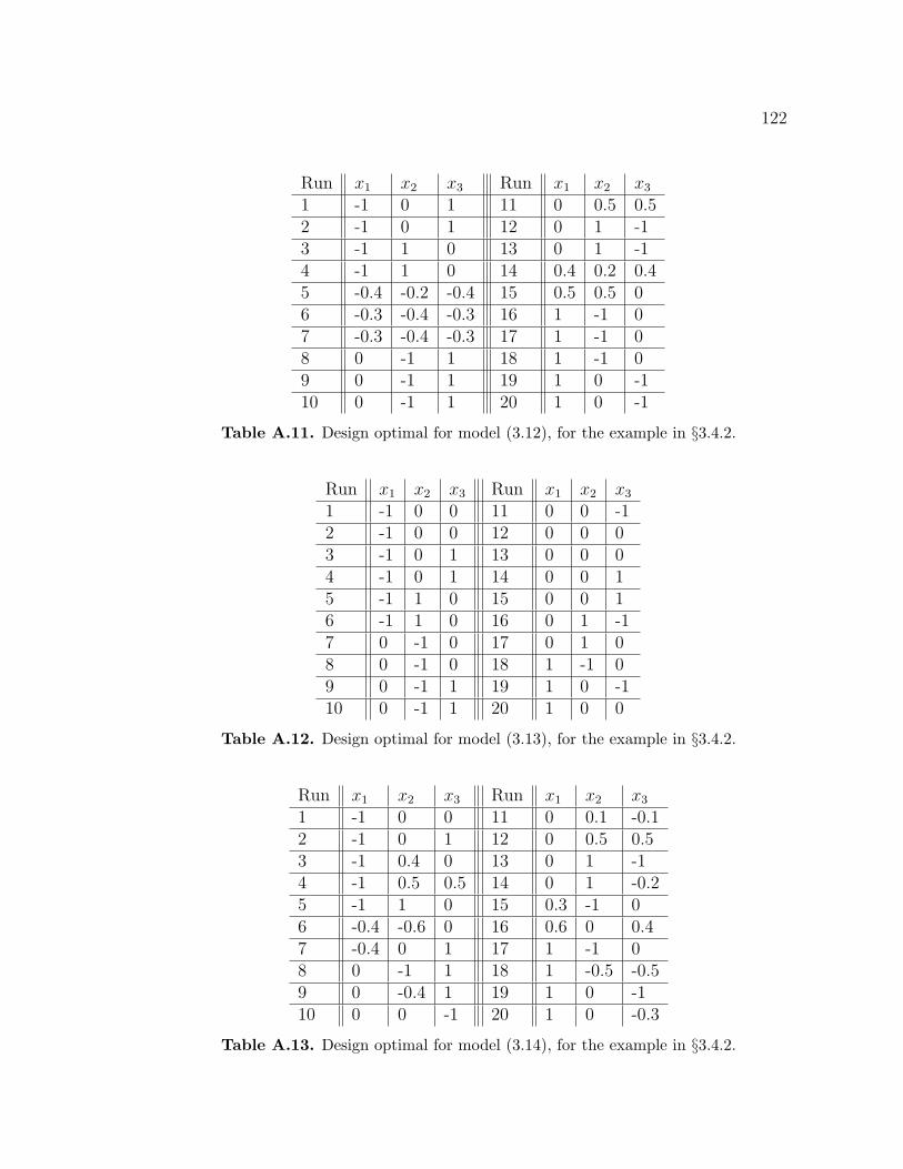
122
Run x1 x2 x3 Run x1 x2 x3
1 -1 0 1 11 0 0.5 0.52 -1 0 1 12 0 1 -13 -1 1 0 13 0 1 -14 -1 1 0 14 0.4 0.2 0.45 -0.4 -0.2 -0.4 15 0.5 0.5 06 -0.3 -0.4 -0.3 16 1 -1 07 -0.3 -0.4 -0.3 17 1 -1 08 0 -1 1 18 1 -1 09 0 -1 1 19 1 0 -110 0 -1 1 20 1 0 -1
Table A.11. Design optimal for model (3.12), for the example in §3.4.2.
Run x1 x2 x3 Run x1 x2 x3
1 -1 0 0 11 0 0 -12 -1 0 0 12 0 0 03 -1 0 1 13 0 0 04 -1 0 1 14 0 0 15 -1 1 0 15 0 0 16 -1 1 0 16 0 1 -17 0 -1 0 17 0 1 08 0 -1 0 18 1 -1 09 0 -1 1 19 1 0 -110 0 -1 1 20 1 0 0
Table A.12. Design optimal for model (3.13), for the example in §3.4.2.
Run x1 x2 x3 Run x1 x2 x3
1 -1 0 0 11 0 0.1 -0.12 -1 0 1 12 0 0.5 0.53 -1 0.4 0 13 0 1 -14 -1 0.5 0.5 14 0 1 -0.25 -1 1 0 15 0.3 -1 06 -0.4 -0.6 0 16 0.6 0 0.47 -0.4 0 1 17 1 -1 08 0 -1 1 18 1 -0.5 -0.59 0 -0.4 1 19 1 0 -110 0 0 -1 20 1 0 -0.3
Table A.13. Design optimal for model (3.14), for the example in §3.4.2.

123
A.3 Designs for Example in §3.4.3
Run x1 x2 x3 x4 Run x1 x2 x3 x4
1 0.66 0.17 0.16 0.01 11 0.65 0 0.35 02 0.5 0 0.475 0.025 12 0.725 0.225 0 0.053 1 0 0 0 13 0.975 0 0 0.0254 0.5 0.225 0.225 0.05 14 0.85 0.15 0 05 0.5 0 0.5 0 15 0.95 0 0 0.056 0.5 0.45 0 0.05 16 0.5 0.5 0 07 0.725 0 0.225 0.05 17 0.5 0.35 0.15 08 0.5 0.15 0.35 0 18 0.85 0 0.15 09 0.5 0.475 0 0.025 19 0.65 0.15 0.16 0.0410 0.65 0.35 0 0 20 0.5 0 0.45 0.05
Table A.14. Model-robust design using the MRMF algorithm, for the example in §3.4.3.
Run x1 x2 x3 x4 Run x1 x2 x3 x4
1 0.5 0.5 0 0 11 0.5 0.1534 0.3466 02 0.5 0.3457 0.1543 0 12 0.5 0.4759 0 0.02413 0.8471 0.1529 0 0 13 0.8444 0 0.1556 04 0.95 0 0 0.05 14 0.5 0.45 0 0.055 0.725 0 0.225 0.05 15 0.6543 0.1544 0.1531 0.03826 0.6550 0.3450 0 0 16 1 0 0 07 0.9759 0 0 0.0241 17 0.5 0 0.4755 0.02458 0.725 0.225 0 0.05 18 0.5 0.225 0.225 0.059 0.6576 0 0.3424 0 19 0.6635 0.1637 0.1640 0.008810 0.5 0 0.5 0 20 0.5 0 0.45 0.05
Table A.15. Model-robust design using the Genetic Algorithm of [54], for the examplein §3.4.3. Note: numbers have been rounded to four decimal places if necessary.

124
Run x1 x2 x3 x4 Run x1 x2 x3 x4
1 0.5 0 0.45 0.05 11 0.64 0.36 0 02 0.5 0 0.475 0.025 12 0.66 0.15 0.15 0.043 0.5 0 0.5 0 13 0.66 0.16 0.17 0.014 0.5 0.14 0.36 0 14 0.725 0 0.225 0.055 0.5 0.225 0.225 0.05 15 0.725 0.225 0 0.056 0.5 0.36 0.14 0 16 0.86 0 0.14 07 0.5 0.45 0 0.05 17 0.86 0.14 0 08 0.5 0.475 0 0.025 18 0.95 0 0 0.059 0.5 0.5 0 0 19 0.975 0 0 0.02510 0.64 0 0.36 0 20 1 0 0 0
Table A.16. Model-robust design using Bayesian method of [37] with 1κ = 1, for the
example in §3.4.3.
Run x1 x2 x3 x4 Run x1 x2 x3 x4
1 0.5 0 0.45 0.05 11 0.64 0.36 0 02 0.5 0 0.475 0.025 12 0.66 0.15 0.15 0.043 0.5 0 0.5 0 13 0.6667 0.1667 0.1667 04 0.5 0.14 0.36 0 14 0.725 0 0.225 0.055 0.5 0.225 0.225 0.05 15 0.725 0.225 0 0.056 0.5 0.36 0.14 0 16 0.86 0 0.14 07 0.5 0.45 0 0.05 17 0.86 0.14 0 08 0.5 0.475 0 0.025 18 0.95 0 0 0.059 0.5 0.5 0 0 19 0.975 0 0 0.02510 0.64 0 0.36 0 20 1 0 0 0
Table A.17. Model-robust design using Bayesian method of [37] with 1κ = 16, for the
example in §3.4.3.
Run x1 x2 x3 x4 Run x1 x2 x3 x4
1 0.5 0 0.45 0.05 11 0.64 0.36 0 02 0.5 0 0.475 0.025 12 0.65 0.16 0.15 0.043 0.5 0 0.5 0 13 0.67 0.16 0.16 0.014 0.5 0.14 0.36 0 14 0.725 0 0.225 0.055 0.5 0.225 0.225 0.05 15 0.725 0.225 0 0.056 0.5 0.36 0.14 0 16 0.86 0 0.14 07 0.5 0.45 0 0.05 17 0.86 0.14 0 08 0.5 0.475 0 0.025 18 0.95 0 0 0.059 0.5 0.5 0 0 19 0.975 0 0 0.02510 0.64 0 0.36 0 20 1 0 0 0
Table A.18. Optimal design for model (3.19), for the example in §3.4.3.

125
Run x1 x2 x3 x4 Run x1 x2 x3 x4
1 0.5 0 0.45 0.05 11 0.5 0.5 0 02 0.5 0 0.45 0.05 12 0.5 0.5 0 03 0.5 0 0.45 0.05 13 0.5 0.5 0 04 0.5 0 0.5 0 14 0.5 0.5 0 05 0.5 0 0.5 0 15 0.95 0 0 0.056 0.5 0 0.5 0 16 0.95 0 0 0.057 0.5 0 0.5 0 17 0.95 0 0 0.058 0.5 0.45 0 0.05 18 1 0 0 09 0.5 0.45 0 0.05 19 1 0 0 010 0.5 0.45 0 0.05 20 1 0 0 0
Table A.19. Optimal design for model (3.16), for the example in §3.4.3.
Run x1 x2 x3 x4 Run x1 x2 x3 x4
1 0.5 0 0.45 0.05 11 0.7375 0 0.2375 0.0252 0.5 0 0.45 0.05 12 0.7375 0.2375 0 0.0253 0.5 0 0.5 0 13 0.75 0 0.2 0.054 0.5 0 0.5 0 14 0.75 0 0.25 05 0.5 0.2375 0.2375 0.025 15 0.75 0.2 0 0.056 0.5 0.25 0.25 0 16 0.75 0.25 0 07 0.5 0.45 0 0.05 17 0.95 0 0 0.058 0.5 0.45 0 0.05 18 0.97 0 0 0.039 0.5 0.5 0 0 19 1 0 0 010 0.5 0.5 0 0 20 1 0 0 0
Table A.20. Optimal design for model (3.17), for the example in §3.4.3.

126
Run x1 x2 x3 x4 Run x1 x2 x3 x4
1 0.5 0 0.45 0.05 11 0.67 0.16 0.17 02 0.5 0 0.475 0.025 12 0.725 0 0.225 0.053 0.5 0 0.5 0 13 0.725 0.225 0 0.054 0.5 0.225 0.225 0.05 14 0.7375 0 0.2375 0.0255 0.5 0.25 0.25 0 15 0.75 0 0.25 06 0.5 0.45 0 0.05 16 0.75 0.25 0 07 0.5 0.45 0 0.05 17 0.75 0.25 0 08 0.5 0.5 0 0 18 0.95 0 0 0.059 0.5 0.5 0 0 19 0.975 0 0 0.02510 0.65 0.17 0.15 0.03 20 1 0 0 0
Table A.21. Optimal design for model (3.18), for the example in §3.4.3.

127
A.4 Designs for Example in §3.4.4
Run x1 x2 x3 Run x1 x2 x3
1 1 0 0 7 0.5 0.5 02 0.5 0.5 0 8 0 0.5 0.53 0 0 1 9 1/3 1/3 1/34 0 1 0 10 1 0 05 0 0 1 11 0 1 06 0.5 0 0.5
Table A.22. Design constructed using the MRMF algorithm, for the example in §3.4.4.
Run x1 x2 x3 Run x1 x2 x3
1 1 0 0 7 1/3 1/3 1/32 0 1 0 8 2/3 1/6 1/63 0 0 1 9 1/6 2/3 1/64 0.5 0.5 0 10 1/6 1/6 2/35 0.5 0 0.5 11 1/3 1/3 1/36 0 0.5 0.5
Table A.23. Design used by Frisbee and McGinity [42], for the example in §3.4.4.
Run x1 x2 x3 Run x1 x2 x3
1 0 1 0 7 0 0 12 0 1 0 8 0 0 13 1 0 0 9 0 1 04 1 0 0 10 0 1 05 1 0 0 11 0 0 16 0 0 1
Table A.24. Design optimal for model (3.20), for the example in §3.4.4.
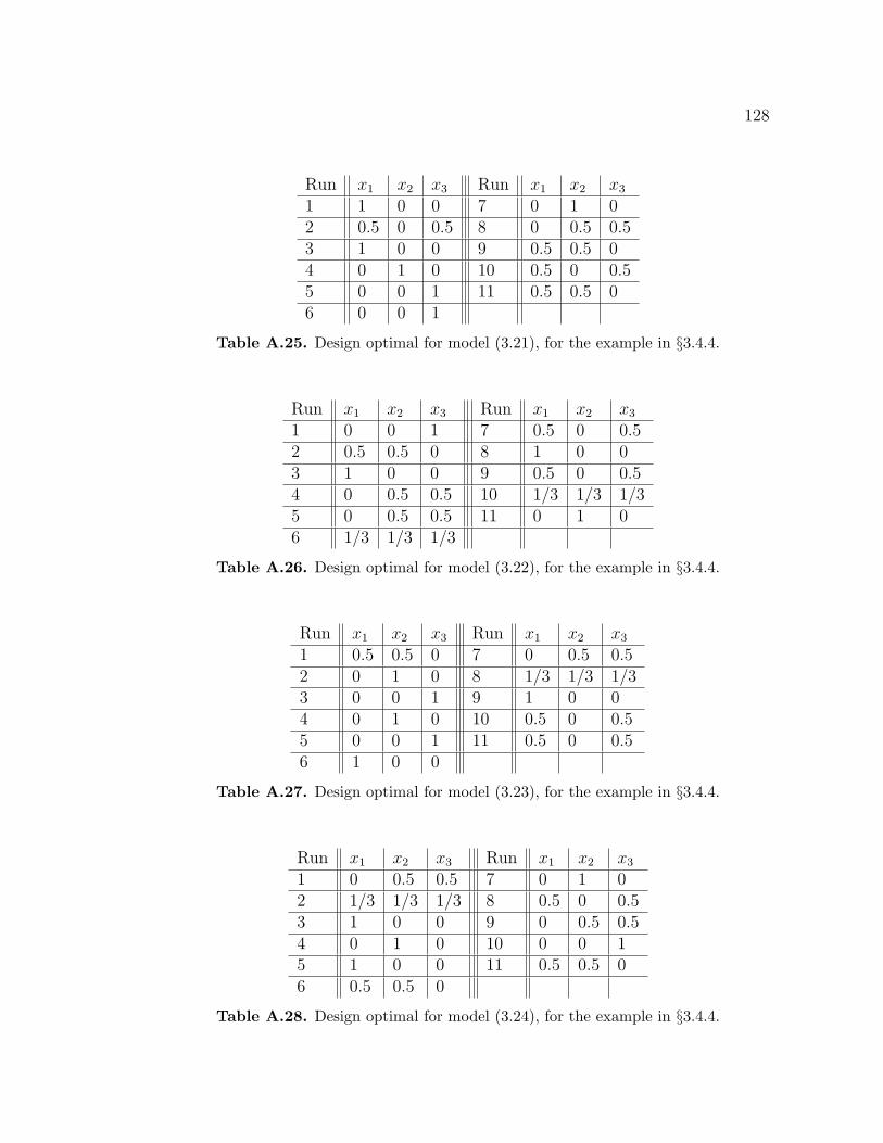
128
Run x1 x2 x3 Run x1 x2 x3
1 1 0 0 7 0 1 02 0.5 0 0.5 8 0 0.5 0.53 1 0 0 9 0.5 0.5 04 0 1 0 10 0.5 0 0.55 0 0 1 11 0.5 0.5 06 0 0 1
Table A.25. Design optimal for model (3.21), for the example in §3.4.4.
Run x1 x2 x3 Run x1 x2 x3
1 0 0 1 7 0.5 0 0.52 0.5 0.5 0 8 1 0 03 1 0 0 9 0.5 0 0.54 0 0.5 0.5 10 1/3 1/3 1/35 0 0.5 0.5 11 0 1 06 1/3 1/3 1/3
Table A.26. Design optimal for model (3.22), for the example in §3.4.4.
Run x1 x2 x3 Run x1 x2 x3
1 0.5 0.5 0 7 0 0.5 0.52 0 1 0 8 1/3 1/3 1/33 0 0 1 9 1 0 04 0 1 0 10 0.5 0 0.55 0 0 1 11 0.5 0 0.56 1 0 0
Table A.27. Design optimal for model (3.23), for the example in §3.4.4.
Run x1 x2 x3 Run x1 x2 x3
1 0 0.5 0.5 7 0 1 02 1/3 1/3 1/3 8 0.5 0 0.53 1 0 0 9 0 0.5 0.54 0 1 0 10 0 0 15 1 0 0 11 0.5 0.5 06 0.5 0.5 0
Table A.28. Design optimal for model (3.24), for the example in §3.4.4.

Appendix BProof of Results in Chapter 4
B.1 Preliminaries
Fedorov [41, Lemma 2.2.2] shows that log(|Mf (ξ)|) is strictly concave. Conse-
quently, we can show that log(Df (ξ)) = 1p
(log(|Mf (ξ)|)− log(|Mf (ξ∗)|)) as well
as minf∈F log(Df (ξ)) are also strictly concave.
Lemma 1. h1(Mf (ξ)) = 1p
(log(|Mf (ξ)|)− log(|Mf (ξ∗)|)) is a strictly concave
function.
Proof. Let ξ∗ be the optimal design for model f . We must show that for any two
arbitrary designs ξ1 and ξ2,
1
p(log |(1− α)Mf (ξ1) + αMf (ξ2)| − log |Mf (ξ
∗)|) >
1− αp
(log |Mf (ξ1)| − log |Mf (ξ∗)|) +
α
p(log |Mf (ξ2)| − log |Mf (ξ
∗)|) .
Since log(|M(ξ)|) is strictly concave, we have that
1
p(log |(1− α)Mf (ξ1) + αMf (ξ2)| − log |Mf (ξ
∗)|)
>1
p((1− α) log |Mf (ξ1)|+ α log |Mf (ξ2)| − log |Mf (ξ
∗)|)
=1− αp
log |Mf (ξ1)|+ α
plog |Mf (ξ2)| − 1
plog |Mf (ξ
∗)|
=1− αp
(log |Mf (ξ1)| − log |Mf (ξ∗)|) +
α
p(log |Mf (ξ2)| − log |Mf (ξ
∗)|)

130
Therefore, h1(Mf (ξ)) is strictly concave.
Lemma 2. Let a1, . . . , ar, ar+1 and b1, . . . , br, br+1 be real numbers. Then,
min(a1, . . . , ar, ar+1) + min(b1, . . . , br, br+1) ≤ min(a1 + b1, . . . , ar + br, ar+1 + br+1)
(B.1)
Proof. We prove by induction. When r = 1, the result is trivially true. Then,
assume
min(a1, . . . , ar) + min(b1, . . . , br) ≤ min(a1 + b1, . . . , ar + br), (B.2)
and show it is true for r + 1. We break it into four cases. Case 1:
min(a1, . . . , ar) ≤ ar+1, min(b1, . . . , br) ≤ br+1 (B.3)
Thus,
min(a1, . . . , ar, ar+1) + min(b1, . . . , br, br+1)
= min(min(a1, . . . , ar), ar+1) + min(min(b1, . . . , br), br+1)
= min(a1, . . . , ar) + min(b1, . . . , br) (B.4)
= min(min(a1, . . . , ar) + min(b1, . . . , br), ar+1 + br+1) (B.5)
≤ min(min(a1 + b1, . . . , ar + br), ar+1 + br+1) (B.6)
= min(a1 + b1, . . . , ar + br, ar+1 + br+1) (B.7)
where (B.4) and (B.5) are true because of (B.3), and the inequality in (B.6) is due
to (B.2). Case 2:
min(a1, . . . , ar) ≤ ar+1, min(b1, . . . , br) > br+1 (B.8)
so that
min(a1, . . . , ar, ar+1) + min(b1, . . . , br, br+1)
= min(min(a1, . . . , ar), ar+1) + min(min(b1, . . . , br), br+1)
= min(a1, . . . , ar) + br+1 (B.9)
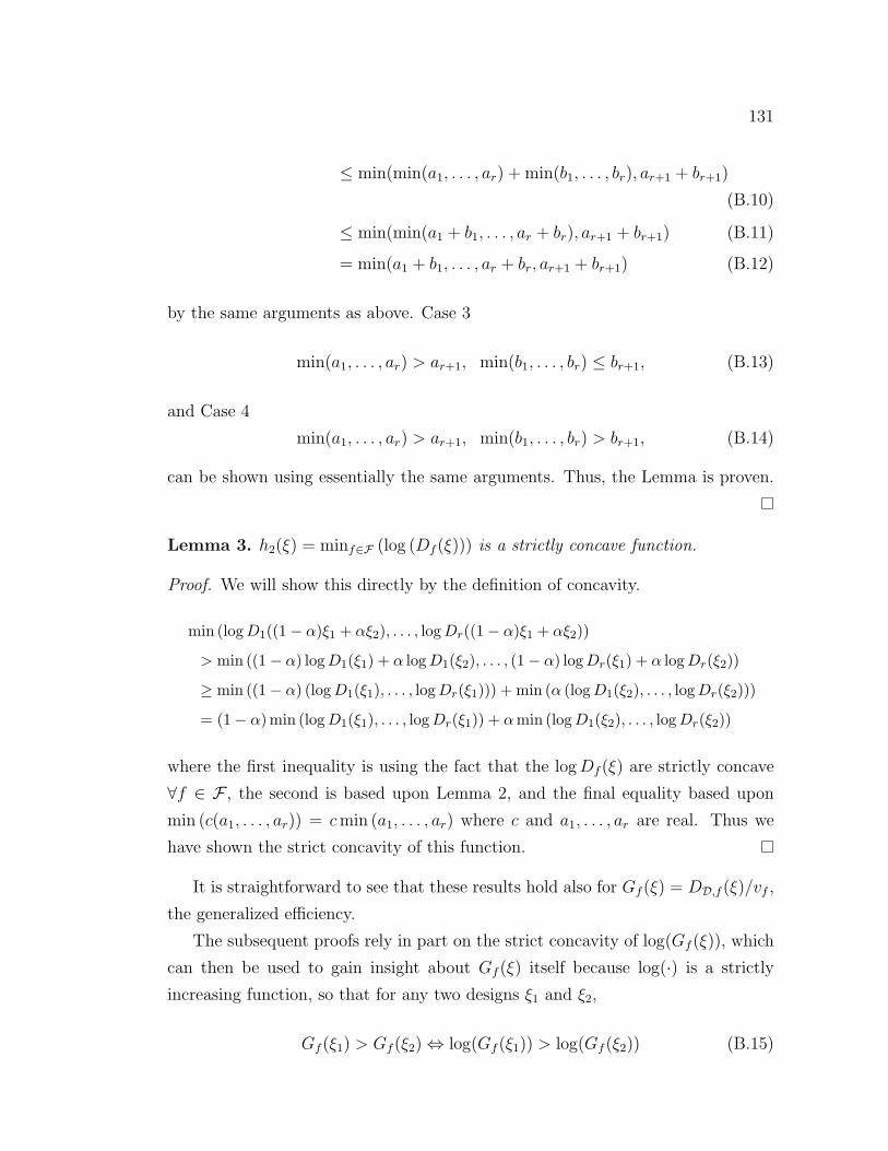
131
≤ min(min(a1, . . . , ar) + min(b1, . . . , br), ar+1 + br+1)
(B.10)
≤ min(min(a1 + b1, . . . , ar + br), ar+1 + br+1) (B.11)
= min(a1 + b1, . . . , ar + br, ar+1 + br+1) (B.12)
by the same arguments as above. Case 3
min(a1, . . . , ar) > ar+1, min(b1, . . . , br) ≤ br+1, (B.13)
and Case 4
min(a1, . . . , ar) > ar+1, min(b1, . . . , br) > br+1, (B.14)
can be shown using essentially the same arguments. Thus, the Lemma is proven.
Lemma 3. h2(ξ) = minf∈F (log (Df (ξ))) is a strictly concave function.
Proof. We will show this directly by the definition of concavity.
min (logD1((1− α)ξ1 + αξ2), . . . , logDr((1− α)ξ1 + αξ2))
> min ((1− α) logD1(ξ1) + α logD1(ξ2), . . . , (1− α) logDr(ξ1) + α logDr(ξ2))
≥ min ((1− α) (logD1(ξ1), . . . , logDr(ξ1))) + min (α (logD1(ξ2), . . . , logDr(ξ2)))
= (1− α) min (logD1(ξ1), . . . , logDr(ξ1)) + αmin (logD1(ξ2), . . . , logDr(ξ2))
where the first inequality is using the fact that the logDf (ξ) are strictly concave
∀f ∈ F , the second is based upon Lemma 2, and the final equality based upon
min (c(a1, . . . , ar)) = cmin (a1, . . . , ar) where c and a1, . . . , ar are real. Thus we
have shown the strict concavity of this function.
It is straightforward to see that these results hold also for Gf (ξ) = DD,f (ξ)/vf ,
the generalized efficiency.
The subsequent proofs rely in part on the strict concavity of log(Gf (ξ)), which
can then be used to gain insight about Gf (ξ) itself because log(·) is a strictly
increasing function, so that for any two designs ξ1 and ξ2,
Gf (ξ1) > Gf (ξ2)⇔ log(Gf (ξ1)) > log(Gf (ξ2)) (B.15)

132
A direct, and useful, consequence of (B.15) is:
minf∈F
Gf (ξ1) > minf∈F
Gf (ξ2)⇔ minf∈F
log(Gf (ξ1)) > minf∈F
log(Gf (ξ2)) (B.16)
B.2 Proof of Theorem 1
Proof. We prove by contradiction. Assume that for design ξ∗, Gf (ξ∗)−Gfmin
(ξ∗) >
0 for all f ∈ F\fmin. Let fg = arg minf∈F\fminGf (ξ
∗) and Gfg(ξ∗) − Gfmin(ξ∗) =
c > 0.
By the strict concavity of log(Gf (·)), and since we assume that ξ∗ is not optimal
for fmin, there exists a direction d = (λ1, . . . , λd) s.t. for an infinitesimal step we
have a new design ξ′for which log(Gfmin
(ξ′)) > log(Gfmin
(ξ∗)). By the equivalence
in (B.15), we have that Gfmin(ξ′) > Gfmin
(ξ∗). Note that without loss of generality,
this new design could exclude design points in or include design points not in ξ∗.
Then by the maximin optimality of ξ∗, Gf (ξ′) for some f ∈ F\fmin must be
reduced by at least c (otherwise, there would exist a larger minimum so that ξ∗
would not be maximin optimal).
Now, with the information matrix as in (4.5), an arbitrarily small step in direc-
tion d results in arbitrarily small changes in ξ∗ in terms of design measures λi for all
i so that the elements of M are negligibly changed, and by the continuity of |·| with
respect to the elements of the matrix, |M| only changes negligibly, say δ < c. But
if δ < c, then ξ∗ is not maximin optimal because minf∈F Gf (ξ′) > minf∈F Gf (ξ
∗).
Since we assumed ξ∗ is maximin optimal, this is a contradiction. Thus the assertion
holds.
B.3 Proof of Theorem 2
Proof. Proof is by contradiction, similar to that for Theorem 1. Assume that for
the generalized maximin optimal design ξ∗, Gf (ξ∗)−Gfmin
(ξ∗) > 0 for some f ∈ F ,
a subset of models which we denote Fg. Let Fl = F\Fg. Then, among all f ∈ Fg,let fg = arg minf∈Fg
Gf (ξ∗) and Gfg(ξ∗)−Gfmin
(ξ∗) = c > 0.

133
Since Fl ⊂ F , condition (4.7) gives that there exists a design ξ′s.t.
minf∈Fl
Gf (ξ′) > min
f∈Fl
Gf (ξ∗).
By the equivalence in (B.16),
minf∈Fl
log(Gf (ξ′)) > min
f∈Fl
log(Gf (ξ∗)).
Since minf∈Fllog(Gf (·)) is strictly concave and, evaluated at ξ∗, is not at its
maximum, there exists a direction d = (λ1, . . . , λd) s.t. for an infinitesimal step
we have a new design, ξ, for which minf∈Fllog(Gf (ξ)) > minf∈Fl
log(Gf (ξ∗)). By
(B.16) again, we have that minf∈FlGf (ξ) > minf∈Fl
Gf (ξ∗). The remainder follows
by the same arguments as the previous proof.
B.4 Proof of Corollary 1
Proof. We have that minf∈F Gf (ξ∗) < 1 because we assume that ξ∗ 6= ξ∗f1 and
ξ∗ 6= ξ∗f2 and that v1 = 1 or v2 = 1. Then, (4.7) is satisfied because we can always
find a direction such that the minimum generalized efficiency is improved for the
model associated with the smaller generalized efficiency. Then, we can use the
same arguments as in the previous results.

Appendix CDesigns for Chapter 4
C.1 Designs for Example in §4.4.1
In this section, we give only the maximin and (1, 1, .6)-maximin designs, since the
others referred to in Table 4.1 are given in Appendix A, Tables A.1-A.5.
Run x1 x2
1 -0.3 02 1 -0.93 0 14 1 05 0.5 -16 -1 1
Table C.1. Maximin model-robust design, for the example in §4.4.1.
Run x1 x2
1 0.5 -12 1 03 -0.6 0.14 -1 15 0 16 1 -1
Table C.2. (1, 1, .6)-Maximin model-robust design, for the example in §4.4.1.

135
C.2 Designs for Example in §4.4.2
Run x1 x2 x3 x4 x5
1 0.6 0.05 0.15 0.15 0.052 0.64 0.05 0.05 0.18 0.083 0.6 0.05 0.095 0.105 0.154 0.64 0.05 0.05 0.25 0.015 0.645 0.05 0.095 0.21 06 0.55 0.1 0.15 0.1 0.17 0.62 0.15 0.05 0.1 0.088 0.57 0.15 0.1 0.1 0.089 0.57 0.1 0.07 0.11 0.1510 0.62 0.05 0.15 0.1 0.0811 0.5 0.15 0.1 0.25 012 0.52 0.15 0.15 0.18 013 0.6 0.05 0.15 0.2 014 0.7 0.07 0.05 0.1 0.0815 0.5 0.15 0.09 0.11 0.1516 0.55 0.15 0.05 0.1 0.1517 0.5 0.15 0.15 0.1 0.118 0.54 0.15 0.05 0.25 0.0119 0.66 0.11 0.05 0.18 020 0.5 0.15 0.09 0.18 0.0821 0.538 0.15 0.1 0.212 022 0.7 0.05 0.05 0.2 023 0.65 0.05 0.05 0.1 0.1524 0.62 0.15 0.05 0.14 0.0425 0.66 0.05 0.11 0.18 0
Table C.3. Maximin model-robust design, for the example in §4.4.2.

136
Run x1 x2 x3 x4 x5
1 0.5 0.15 0.1 0.25 02 0.6 0.05 0.1 0.25 03 0.62 0.15 0.05 0.18 04 0.5 0.15 0.15 0.1 0.15 0.5 0.15 0.15 0.15 0.056 0.7 0.07 0.05 0.1 0.087 0.52 0.15 0.15 0.18 08 0.7 0.05 0.05 0.15 0.059 0.55 0.15 0.05 0.25 010 0.52 0.15 0.07 0.11 0.1511 0.57 0.15 0.1 0.1 0.0812 0.65 0.05 0.05 0.1 0.1513 0.62 0.05 0.15 0.18 014 0.6 0.05 0.09 0.18 0.0815 0.55 0.1 0.15 0.2 016 0.632 0.094 0.094 0.18 017 0.538 0.15 0.1 0.212 018 0.6 0.05 0.15 0.1 0.119 0.54 0.15 0.05 0.18 0.0820 0.7 0.05 0.05 0.2 021 0.585 0.15 0.05 0.1 0.11522 0.55 0.1 0.09 0.11 0.1523 0.64 0.05 0.05 0.25 0.0124 0.66 0.11 0.05 0.1 0.0825 0.66 0.05 0.11 0.1 0.08
Table C.4. (.9,1,1)-maximin model-robust design, for the example in §4.4.2.

137
Run x1 x2 x3 x4 x5
1 0.54 0.15 0.05 0.18 0.082 0.65 0.05 0.05 0.1 0.153 0.5 0.15 0.15 0.1 0.14 0.62 0.15 0.05 0.1 0.085 0.57 0.15 0.1 0.18 06 0.6 0.05 0.09 0.11 0.157 0.55 0.15 0.05 0.25 08 0.57 0.1 0.15 0.18 09 0.64 0.05 0.05 0.25 0.0110 0.5 0.15 0.09 0.25 0.0111 0.62 0.15 0.05 0.18 012 0.6 0.05 0.15 0.1 0.113 0.52 0.15 0.15 0.1 0.0814 0.7 0.07 0.05 0.1 0.0815 0.62 0.05 0.15 0.18 016 0.66 0.05 0.11 0.1 0.0817 0.6 0.05 0.09 0.18 0.0818 0.7 0.07 0.05 0.18 019 0.7 0.05 0.05 0.2 020 0.5963 0.095 0.0875 0.1606 0.0606221 0.6 0.05 0.1 0.25 022 0.5 0.15 0.15 0.2 023 0.5 0.15 0.095 0.105 0.1524 0.55 0.15 0.05 0.1 0.1525 0.57 0.1 0.07 0.25 0.01
Table C.5. (.9,1,.5)-maximin model-robust design, for the example in §4.4.2.
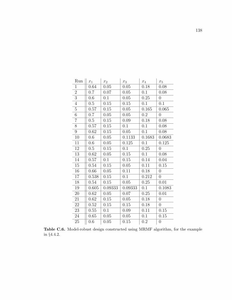
138
Run x1 x2 x3 x4 x5
1 0.64 0.05 0.05 0.18 0.082 0.7 0.07 0.05 0.1 0.083 0.6 0.1 0.05 0.25 04 0.5 0.15 0.15 0.1 0.15 0.57 0.15 0.05 0.165 0.0656 0.7 0.05 0.05 0.2 07 0.5 0.15 0.09 0.18 0.088 0.57 0.15 0.1 0.1 0.089 0.62 0.15 0.05 0.1 0.0810 0.6 0.05 0.1133 0.1683 0.068311 0.6 0.05 0.125 0.1 0.12512 0.5 0.15 0.1 0.25 013 0.62 0.05 0.15 0.1 0.0814 0.57 0.1 0.15 0.14 0.0415 0.54 0.15 0.05 0.11 0.1516 0.66 0.05 0.11 0.18 017 0.538 0.15 0.1 0.212 018 0.54 0.15 0.05 0.25 0.0119 0.605 0.09333 0.09333 0.1 0.108320 0.62 0.05 0.07 0.25 0.0121 0.62 0.15 0.05 0.18 022 0.52 0.15 0.15 0.18 023 0.55 0.1 0.09 0.11 0.1524 0.65 0.05 0.05 0.1 0.1525 0.6 0.05 0.15 0.2 0
Table C.6. Model-robust design constructed using MRMF algorithm, for the examplein §4.4.2.
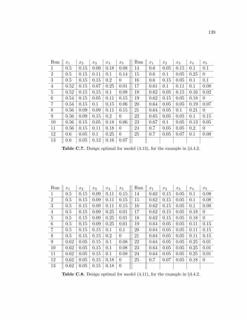
139
Run x1 x2 x3 x4 x5 Run x1 x2 x3 x4 x5
1 0.5 0.15 0.09 0.18 0.08 14 0.6 0.05 0.15 0.1 0.12 0.5 0.15 0.11 0.1 0.14 15 0.6 0.1 0.05 0.25 03 0.5 0.15 0.15 0.2 0 16 0.6 0.15 0.05 0.1 0.14 0.52 0.15 0.07 0.25 0.01 17 0.61 0.1 0.11 0.1 0.085 0.52 0.15 0.15 0.1 0.08 18 0.62 0.05 0.15 0.16 0.026 0.54 0.15 0.05 0.11 0.15 19 0.62 0.15 0.05 0.18 07 0.54 0.15 0.1 0.15 0.06 20 0.64 0.05 0.05 0.19 0.078 0.56 0.09 0.09 0.11 0.15 21 0.64 0.05 0.1 0.21 09 0.56 0.09 0.15 0.2 0 22 0.65 0.05 0.05 0.1 0.1510 0.56 0.15 0.05 0.18 0.06 23 0.67 0.1 0.05 0.13 0.0511 0.56 0.15 0.11 0.18 0 24 0.7 0.05 0.05 0.2 012 0.6 0.05 0.1 0.25 0 25 0.7 0.05 0.07 0.1 0.0813 0.6 0.05 0.12 0.16 0.07
Table C.7. Design optimal for model (4.13), for the example in §4.4.2.
Run x1 x2 x3 x4 x5 Run x1 x2 x3 x4 x5
1 0.5 0.15 0.09 0.11 0.15 14 0.62 0.15 0.05 0.1 0.082 0.5 0.15 0.09 0.11 0.15 15 0.62 0.15 0.05 0.1 0.083 0.5 0.15 0.09 0.11 0.15 16 0.62 0.15 0.05 0.1 0.084 0.5 0.15 0.09 0.25 0.01 17 0.62 0.15 0.05 0.18 05 0.5 0.15 0.09 0.25 0.01 18 0.62 0.15 0.05 0.18 06 0.5 0.15 0.09 0.25 0.01 19 0.64 0.05 0.05 0.11 0.157 0.5 0.15 0.15 0.1 0.1 20 0.64 0.05 0.05 0.11 0.158 0.5 0.15 0.15 0.2 0 21 0.64 0.05 0.05 0.11 0.159 0.62 0.05 0.15 0.1 0.08 22 0.64 0.05 0.05 0.25 0.0110 0.62 0.05 0.15 0.1 0.08 23 0.64 0.05 0.05 0.25 0.0111 0.62 0.05 0.15 0.1 0.08 24 0.64 0.05 0.05 0.25 0.0112 0.62 0.05 0.15 0.18 0 25 0.7 0.07 0.05 0.18 013 0.62 0.05 0.15 0.18 0
Table C.8. Design optimal for model (4.11), for the example in §4.4.2.

140
Run x1 x2 x3 x4 x5 Run x1 x2 x3 x4 x5
1 0.5 0.15 0.09 0.11 0.15 14 0.6 0.05 0.1 0.25 02 0.5 0.15 0.09 0.25 0.01 15 0.6 0.05 0.15 0.1 0.13 0.5 0.15 0.15 0.1 0.1 16 0.6 0.05 0.15 0.2 04 0.5 0.15 0.15 0.2 0 17 0.62 0.05 0.15 0.1 0.085 0.54 0.15 0.05 0.18 0.08 18 0.62 0.15 0.05 0.1 0.086 0.55 0.15 0.05 0.1 0.15 19 0.62 0.15 0.05 0.18 07 0.56 0.09 0.1 0.1 0.15 20 0.64 0.05 0.05 0.11 0.158 0.56 0.11 0.15 0.18 0.18 21 0.65 0.05 0.05 0.25 09 0.56 0.15 0.11 0.1 0.08 22 0.67 0.05 0.1 0.18 010 0.58 0.15 0.05 0.22 0 23 0.69 0.05 0.05 0.1 0.1111 0.59 0.1 0.05 0.25 0.01 24 0.7 0.07 0.05 0.1 0.0812 0.59 0.1 0.09 0.16 0.06 25 0.7 0.07 0.05 0.18 013 0.6 0.05 0.09 0.18 0.08
Table C.9. Design optimal for model (4.12), for the example in §4.4.2.

141
C.3 Designs for Example in §4.4.3
In this section, we give only the maximin and (.9, 1, 1, 1, .9)-maximin designs, since
the others referred to in Table 4.3 are given in Appendix A, Tables 3.4-A.28.
Run x1 x2 x3 Run x1 x2 x3
1 0 0.5 0.5 7 1 0 02 0 0 1 8 1/3 1/3 1/33 0 1 0 9 0 1 04 0 0 1 10 5/12 0 7/125 1 0 0 11 1 0 06 1/3 2/3 0
Table C.10. Maximin model-robust design, for the example in §4.4.3.
Run x1 x2 x3 Run x1 x2 x3
1 0 1 0 7 0 0 12 0.5 0.5 0 8 1 0 03 0 0 1 9 7/12 0 5/124 1 0 0 10 1/3 5/12 1/45 0 1 0 11 0 0 16 0 0.5 0.5
Table C.11. (.9,1,1,1,.9)-maximin model-robust design, for the example in §4.4.3.

Appendix DMatrix Algebra Results for Chapter 5
We provide here a collection of results which are necessary to prove Theorem 3
and Corollary 2. The first is well-known and presented without proof.
Lemma 4. Let ∆ be a block matrix such that
∆ =
(∆11 ∆12
∆21 ∆22
), (D.1)
where ∆11 is a n × n nonsingular matrix, ∆12 is a n × k matrix, ∆21 is a k × nmatrix, and ∆22 is a k × k nonsingular matrix. Then
|∆| = |∆11||∆22 −∆21∆−111 ∆12| = |∆11 −∆12∆
−122 ∆21||∆22|. (D.2)
The next result is a slight generalization of an identity given in Schott [93].
Lemma 5. Let M be n× n, A be n× k and B be k × n. Then
|M + AB| =
∣∣∣∣∣M A
−B Ik
∣∣∣∣∣ . (D.3)
Proof. Using basic matrix multiplication, it is true that(M A
−B Ik
)(In 0
B Ik
)=
(M + AB A
0 Ik
). (D.4)
Taking the determinant of both sides, and using the well known property that the

143
determinant of a product of two matrices is equal to the product of the determi-
nants of the matrices, gives∣∣∣∣∣M A
−B Ik
∣∣∣∣∣∣∣∣∣∣In 0
B Ik
∣∣∣∣∣ =
∣∣∣∣∣M + AB A
0 Ik
∣∣∣∣∣ , (D.5)
and by Lemma 4, ∣∣∣∣∣In 0
B Ik
∣∣∣∣∣ = |In||Ik − 0| = 1. (D.6)
Thus, ∣∣∣∣∣M A
−B Ik
∣∣∣∣∣ =
∣∣∣∣∣M + AB A
0 Ik
∣∣∣∣∣= |In||M + AB−AIk0|
= |M + AB|,
where the second equality follows from another appeal to Lemma 4.
Another identity simply combines the two previous results and is a slight gen-
eralization of Lemma 2.5.1 in Fedorov [41].
Lemma 6. Let M be a nonsingular n× n matrix, let A be a n× k matrix and let
B be an k × n matrix; then
|M + AB| = |M||Ik + BM−1A|. (D.7)
Proof. Lemma 5 gives that
|M + AB| =
∣∣∣∣∣M A
−B Ik
∣∣∣∣∣ . (D.8)
and then by Lemma 4 we get what we wanted to prove.
Finally, a useful and well-known result ([41], Lemma 2.6.1) is the Matrix In-
version Lemma.

144
Lemma 7. Let A be a n× k matrix and let B be an k × n matrix; then
(In + AB)−1 = In −A(Ik + BA)−1B. (D.9)

Appendix EDesigns for Chapter 5
E.1 Designs for Example in §5.5.1
Run x1 x2 x3 Run x1 x2 x3
1 1.73 -1.73 -1.73 11 -1.73 -1.73 1.732 -1.73 1.73 -1.73 12 -1.73 -1.73 -1.733 1.73 -1.73 1.73 13 0 -1.73 04 -1.73 1.73 1.73 14 1.73 -1.73 -1.735 -1.73 -1.73 1.73 15 0 1.73 -1.736 1.73 1.73 1.73 16 1.73 1.73 -1.737 0 1.73 1.73 17 -1.73 0 08 -1.73 1.73 0 18 1.73 1.73 09 1.73 0 1.73 19 -1.73 -1.73 -1.7310 0 -1.73 0 20 0 0 -1.73
Table E.1. D-optimal design constructed via MX algorithm, for example in §5.5.1,when Σ and ρ(x) are known
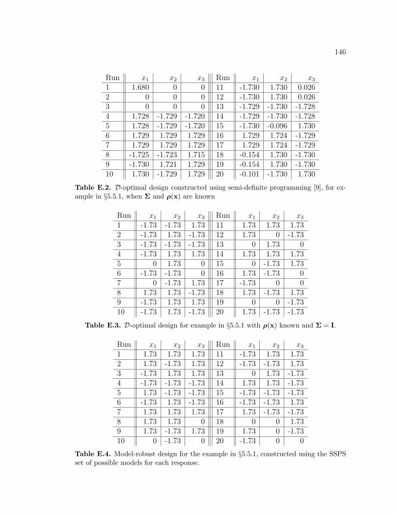
146
Run x1 x2 x3 Run x1 x2 x3
1 1.680 0 0 11 -1.730 1.730 0.0262 0 0 0 12 -1.730 1.730 0.0263 0 0 0 13 -1.729 -1.730 -1.7284 1.728 -1.729 -1.720 14 -1.729 -1.730 -1.7285 1.728 -1.729 -1.720 15 -1.730 -0.096 1.7306 1.729 1.729 1.729 16 1.729 1.724 -1.7297 1.729 1.729 1.729 17 1.729 1.724 -1.7298 -1.725 -1.723 1.715 18 -0.154 1.730 -1.7309 -1.730 1.721 1.729 19 -0.154 1.730 -1.73010 1.730 -1.729 1.729 20 -0.101 -1.730 1.730
Table E.2. D-optimal design constructed using semi-definite programming [9], for ex-ample in §5.5.1, when Σ and ρ(x) are known
Run x1 x2 x3 Run x1 x2 x3
1 -1.73 -1.73 1.73 11 1.73 1.73 1.732 -1.73 1.73 -1.73 12 1.73 0 -1.733 -1.73 -1.73 -1.73 13 0 1.73 04 -1.73 1.73 1.73 14 1.73 1.73 1.735 0 1.73 0 15 0 -1.73 1.736 -1.73 -1.73 0 16 1.73 -1.73 07 0 -1.73 1.73 17 -1.73 0 08 1.73 1.73 -1.73 18 1.73 -1.73 1.739 -1.73 1.73 1.73 19 0 0 -1.7310 -1.73 1.73 -1.73 20 1.73 -1.73 -1.73
Table E.3. D-optimal design for example in §5.5.1 with ρ(x) known and Σ = I.
Run x1 x2 x3 Run x1 x2 x3
1 1.73 1.73 1.73 11 -1.73 1.73 1.732 1.73 -1.73 1.73 12 -1.73 -1.73 1.733 -1.73 1.73 1.73 13 0 1.73 -1.734 -1.73 -1.73 -1.73 14 1.73 1.73 -1.735 1.73 -1.73 -1.73 15 -1.73 -1.73 -1.736 -1.73 1.73 -1.73 16 -1.73 -1.73 1.737 1.73 1.73 1.73 17 1.73 -1.73 -1.738 1.73 1.73 0 18 0 0 1.739 1.73 -1.73 1.73 19 1.73 0 -1.7310 0 -1.73 0 20 -1.73 0 0
Table E.4. Model-robust design for the example in §5.5.1, constructed using the SSPSset of possible models for each response.

147
Run x1 x2 x3 Run x1 x2 x3
1 1.73 1.73 1.73 11 -1.73 -1.73 -1.732 1.73 -1.73 -1.73 12 -1.73 1.73 -1.733 1.73 1.73 -1.73 13 1.73 -1.73 -1.734 -1.73 -1.73 -1.73 14 1.73 1.73 1.735 1.73 -1.73 1.73 15 1.73 -1.73 1.736 -1.73 1.73 -1.73 16 -1.73 1.73 1.737 -1.73 -1.73 1.73 17 0 0 -1.738 -1.73 -1.73 1.73 18 0 1.73 09 1.73 -1.73 1.73 19 -1.73 1.73 1.7310 1.73 1.73 -1.73 20 -1.73 0 0
Table E.5. Model-robust design for the example in §5.5.1, constructed using the SPSset of possible models for each response, assuming Σ is known (in this case, the designis the same if we use Σ = I).
Run x1 x2 x3 Run x1 x2 x3
1 1.73 1.73 -1.73 11 0 -1.73 02 1.73 -1.73 1.73 12 -1.73 -1.73 1.733 1.73 1.73 1.73 13 0 1.73 1.734 1.73 0 -1.73 14 -1.73 0 -1.735 -1.73 1.73 -1.73 15 -1.73 1.73 06 1.73 -1.73 1.73 16 1.73 0 07 1.73 1.73 0 17 1.73 -1.73 -1.738 -1.73 -1.73 1.73 18 -1.73 -1.73 -1.739 -1.73 1.73 1.73 19 0 -1.73 -1.7310 0 1.73 -1.73 20 0 0 1.73
Table E.6. D-optimal design for the example in §5.5.1, constructed assuming the fullquadratic model only.

148
E.2 Designs for Example in §5.5.2
Run x1 x2 Run x1 x2
1 -1 -1 7 1 -12 -1 -1 8 1 -13 1 1 9 1 14 -1 1 10 -1 15 0 -1 11 0 16 1 0 12 -1 0
Table E.7. Model-robust design for example in §5.5.2, constructed using the SSPSmodel set (the design constructed using the SPS model set is the same).
Run x1 x2 Run x1 x2
1 0 1 7 -1 02 1 -1 8 0 -13 1 0 9 1 -14 1 1 10 -1 -15 -1 1 11 -1 16 -1 -1 12 0 0
Table E.8. D-optimal design for the example in §5.5.2, constructed assuming the fullquadratic model only.

149
E.3 Designs for Example in §5.5.3
Run x1 x2 x3 Run x1 x2 x3
1 1 -1 0 10 1 -1 12 -1 -1 -1 11 -1 1 03 1 1 -1 12 0 1 04 1 1 0 13 0 -1 15 1 -1 -1 14 -1 1 -16 -1 1 1 15 0 -1 07 -1 -1 0 16 1 1 18 -1 -1 1 17 0 1 -19 0 -1 -1
Table E.9. D-optimal design for example in §5.5.3, with ρ(x) and Σ assumed known.
Run x1 x2 x3 Run x1 x2 x3
1 -1 1 -1 10 -1 0 12 1 1 1 11 0 1 03 -1 -1 -1 12 1 -1 14 1 -1 1 13 1 0 05 -1 1 -1 14 1 1 16 1 1 -1 15 1 -1 -17 -1 1 1 16 0 0 -18 -1 -1 1 17 1 -1 -19 -1 -1 0
Table E.10. Model-robust design for example in §5.5.3, constructed using the SSPSmodel set.

150
Run x1 x2 x3 Run x1 x2 x3
1 -1 1 1 10 -1 -1 -12 1 1 1 11 1 -1 03 -1 -1 1 12 -1 1 -14 1 -1 -1 13 -1 1 -15 1 -1 1 14 0 0 06 1 1 -1 15 0 1 -17 -1 -1 -1 16 -1 -1 18 -1 1 1 17 1 0 -19 1 1 1
Table E.11. Model-robust design for example in §5.5.3, constructed using the SPSmodel set.
Run x1 x2 x3 Run x1 x2 x3
1 1 -1 1 10 -1 -1 12 1 1 1 11 1 -1 -13 -1 1 1 12 1 -1 14 1 1 -1 13 -1 0 -15 -1 1 -1 14 1 1 06 -1 -1 -1 15 -1 1 07 -1 0 0 16 0 1 -18 1 0 -1 17 0 0 19 0 -1 0
Table E.12. D-optimal design for example in §5.5.3, for quadratic model only.

Appendix FUpdating Formulae for Split-Plot
Exchange Algorithms
F.1 Derivation of Convenient Form of the Split-
Plot Information Matrix
In this appendix, we will review the derivation of a particular form of the split-plot
information matrix, for a given model form. Fist, to calculate the inverse of W,
we need a lemma that is given and proven in Miller [78].
Lemma 8. Let G be a nonsingular square matrix and H be a rank one matrix of
the same dimension. Then,
(G + H)−1 = G−1 − 1
1 + gG−1HG−1
where g = tr(HG−1)
Then, as given in Goos and Vandebroek [49], W−1i can be calculated by ap-
pealing to Lemma 8, noting that tr(η1si1′si
) = dsi:
W−1i =
1
σ2ε
(Isi− η
1 + siη1si
1′
si
)

152
Then, because W is block diagonal,
W−1 =
W−1
1 0 . . . 0
0 W−12 . . . 0
......
. . ....
0 0 . . . W−1b
Now, we write
X =
X1
X2
. . .
Xb
where Xi is a si × p matrix:
Xi =
f′(zi,xi1)
f′(zi,xi2)
. . .
f′(zi,xisi
)
Then matrix multiplication shows that the information matrix, Msp, is
Msp = X′W−1X =
(X′1 X
′2 . . . X
′
b
)
W−11 0 . . . 0
0 W−12 . . . 0
......
. . ....
0 0 . . . W−1b
X1
X2
. . .
Xb
=
b∑i=1
X′
iW−1i Xi
It can be shown [49] that
X′V−1X =
1
σ2ε
(b∑i=1
si∑j=1
f(zi,xij)f′(zi,xij)−
b∑i=1
η
1 + siη(X
′
i1si)(X
′
i1si)′
)(F.1)
This is convenient as an update formula for the information matrix. For in-

153
stance, if we want to add a point to the ith whole plot:
Msp = X′W−1X = X
′W−1X + f(zi,xi,si+1)f
′(zi,xi,si+1)
+η
1 + siη(X
′
i1si)(X
′
i1si)′
(F.2)
− η
1 + (si + 1)η(X
′
i1si+1)(X′
i1si+1)′
where the last two parts together give the impact of the additional observation on
the last part of the information matrix in (F.1). We can rewrite (F.2) in the form
R + STU, so that we can use the well-known matrix inversion lemma (see [5]):
(R + STU)−1 = R−1 −R−1S(T−1 + UR−1S
)−1UR−1
where R is r × r, S is r × t, T is t× t and U is t× r. For this case, we have
M = M +
f′(zi,xi,si+1)
(X′i1si
)′
(X′i1si+1)
′
′
1 0 0
0 d1+sid
0
0 0 d1+(si+1)d
f′(zi,xi,si+1)
(X′i1si
)′
(X′i1si+1)
′
= R + STU
so that
M−1 = R−1 −R−1S(T−1 + UR−1S
)−1UR−1.
F.2 Matrix Results Used in Split-Plot Exchange
Algorithms
For reference purposes, we reproduce some results from [5] which speed up our
algorithm. Exchanges in the split-plot situation are more complicated than the
completely randomized scenario because there are several possible types of ex-
changes, each having a different impact upon the determinant and inverse of the
information matrix. In what follows we give updating formulae for the information
matrix, its inverse, and its determinant, for each of the three relevant exchange
scenarios.

154
F.2.1 Updating Formulae for Changes in Easy-to-Change
Factors
First, we consider the case in which a design point is exchanged for a candidate
point, both having the same whole plot factor levels. The design point is (zi,xij),
whereas the candidate point to be exchanged is (zi,x∗ij). It is shown in Arnouts
and Goos [5] that:
Msp = Msp − f(zi,xij)f′(zi,xij) + f(zi,x
∗ij)f
′(zi,x
∗ij)
+η
1 + ηsi
(X′
i1si
)(X′
i1si
)′− η
1 + ηsi
(X′
i1si
)(X′
i1si
)′, (F.3)
∣∣∣Msp
∣∣∣ = |Msp| |D1|∣∣∣D−1
1 + U1M−1sp U
′
1
∣∣∣ (F.4)
and (Msp
)−1
= M−1sp −M−1
sp U′
1
(D−1
1 + U1M−1sp U
′
1
)−1
U1M−1sp (F.5)
where D1 = diag(−1, 1, η
1+siη,− η
1+siη
),
U1 =[f(zi,xij), f(zi,x
∗ij),(X′
i1si
),(X′
i1si
)]′,
|D1| = η2
(1+siη)2, and X
′i1si
= X′i1si− f(zi,xij) + f(zi,x
∗ij).
F.2.2 Swapping Two Points From Different Whole Plots
Another way to perturb a split-plot design is to exchange existing design points
from two different whole plots. To perform such a swap, the whole plot factor
levels for both must be the same (otherwise, the result would be whole plots with
more than one level of whole plot factors). Note that the change does not affect the
quantity X′X because of the simple change in ordering of the two design points.
However, it does affect whole plot part of the information matrix:
Msp = Msp +η
1 + ηsi
(X′
i1si
)(X′
i1si
)′+
η
1 + ηsl
(X′
l1sl
)(X′
l1sl
)′− η
1 + ηsi
(X′
i1si
)(X′
i1si
)′− η
1 + ηsl
(X′
l1sl
)(X′
l1sl
)′, (F.6)

155
∣∣∣Msp
∣∣∣ = |Msp| |D2|∣∣∣D−1
2 + U2M−1sp U
′
2
∣∣∣ (F.7)
and (Msp
)−1
= M−1sp −M−1
sp U′
2
(D−1
2 + U2M−1sp U
′
2
)−1
U2M−1sp (F.8)
where D2 = diag(
η1+siη
, η1+slη
,− η1+siη
,− η1+slη
),
U2 =[(
X′
i1si
),(X′
l1sl
),(X′
i1si
),(X′
l1sl
)],
|D2| = η4
(1+siη)2(1+slη)2, X
′i1si
= X′i1si− f(zi,xij) + f(zl,xlm), and X
′
l1sl= X
′
l1sl−
f(zl,xlm) + f(zi,xij).
F.2.3 Updating Formulae for Changes in Hard-to-Change
Factors
If the levels of the whole plot factors are changed from zi to z∗i for any run ij, the
levels of those factors for all runs in whole plot i will have to be changed as well
because of the restriction that the whole-plot factor levels be the same within a
given whole plot. Arnouts and Goos [5] show that:
Msp = Msp −X′
iXi + X′
iXi
+η
1 + ηsi
(X′
i1si
)(X′
i1si
)′− η
1 + ηsi
(X′
i1si
)(X′
i1si
)′, (F.9)
∣∣∣Msp
∣∣∣ = |Msp| |D3|∣∣∣D−1
3 + U3M−1sp U
′
3
∣∣∣ (F.10)
and (Msp
)−1
= M−1sp −M−1
sp U′
3
(D−1
3 + U3M−1sp U
′
3
)−1
U3M−1sp (F.11)
where D3 = diag(−Isi
, Isi, η
1+siη,− η
1+siη
),
U3 =[X′
i, X′
i,(X′
i1si
),(X′
i1si
)],
|D3| = η3
(1+siη)3(−1)si+1, and X
′i = [f(z∗i ,xi1), . . . , f(z∗i ,xisi
)]′.

Appendix GD-optimal Split-Plot Algorithm of
Goos and Vandebroek [50]
Here we give the original algorithm of [50], generally using the same notation as in
§6.3.2. For the algorithm, we must specify 1) The candidate list, C; 2) the number
of whole plots, b; 3) the size of each whole plot, k1, k2, . . . , kb; and 4) the model
form f′(z,x). Let M∗
sp be the information matrix for the best design found so far.
The algorithm is as follows.
1. Set |M∗sp| = 0, tc = 1.
2. Determine pw, the number of coefficients for whole plot factors only.
3. Determine ps, the number of coefficients for subplot factors only.
4. Set Msp = ωI (where ω is a small constant) and calculate M−1sp ; set Hi = ∅.
5. Construct initial design
(a) Randomly assign pw unique whole-plot factor settings to pw whole plots.
(b) Randomly assign b − pw levels of the whole-plot factors to the rest of
the whole plots.
(c) Randomly choose u (1 ≤ u ≤ p).
(d) Do u times:
i. Randomly select i ∈ B (select a whole plot at random)

157
ii. Randomly select j ∈ Ci (select a candidate point with the ith setting
of whole plot, at random)
iii. If #Hi < ki, then Hi = Hi ∪ j; otherwise, go back to step i.
iv. Update M−1sp via (F.1).
(e) Do n− u times:
i. Set l = 1.
ii. Determine j ∈ C with the lth biggest prediction variance via (6.5).
iii. Find i, where i ∈ B, j ∈ Ci, and #Hi < ki (find a nonfull whole
plot into which j can be inserted). If no such i exists, set l = l + 1
and return to step ii.
iv. Hi = Hi ∪ j.
v. Update M−1sp via (F.1).
6. Compute Msp and |Msp| for the initial design. If |Msp| = 0, go back to step
4. Otherwise, continue.
7. Set ν = 0.
8. Evaluate design point exchanges (swapping design points with candidate
points, where whole plot factors settings are the same):
(a) Set δ = 1.
(b) ∀i ∈ B, ∀j ∈ Hi, ∀k ∈ Ci, j 6= k:
i. Determine the effect δijk = |Mijk,sp|/|Msp| of exchanging, in the ith
whole plot, points j and k, using (F.4).
ii. if δijk > δ, then δ = δijk and store i, j, and k.
9. If δ > 1 + ε, then go to step 10; otherwise, go to step 11.
10. Perform the best exchange:
(a) Hi = Hi \ j ∪ k.
(b) Update M−1sp via (F.5) and |Msp| via (F.4).
(c) Set ν = 1.

158
11. Evaluate interchanges of points within whole plots with the same factor levels
(a) Set δ = 1.
(b) ∀i, j ∈ B, i < j, zi = zj, ∀k ∈ Hi, ∀l ∈ Hj, k 6= l:
i. Determine the effect δjlik = |Mjlik,sp|/|Msp| of moving k to whole plot
j (from whole plot i) and l to whole plot i (from whole plot j), via
(F.7).
ii. If δjlik > δ, then δ = δjlik and store i, j, k, and l.
12. If δ > 1 + ε, go to step 13; otherwise, go to step 14.
13. Perform the best interchange:
(a) Hi = Hi \ k ∪ l.
(b) Hj = Hj \ l ∪ k.
(c) Update M−1sp and |Msp| via (F.7).
(d) Set ν = 1.
14. Evaluate exchanges of whole-plot factor settings:
(a) Set δ = 1.
(b) ∀i ∈ B, ∀j ∈ P , zi 6= zj:
i. Determine the effect δij = |Mij,sp|/|Msp| of exchanging zi by zj in
the ith whole plot, via (F.10).
ii. If δij > δ, then δ = δij and store i and j.
15. If δ > 1 + ε, go to step 16; otherwise, go to step 17.
16. Perform best exchange:
(a) Update Hi and Ci.
(b) Update M−1sp via (F.11) and |Msp| via (F.10).
(c) Set ν = 1.
17. If ν = 1, go to step 7.

159
18. If |Msp| > |M∗sp|, then |M∗
sp| = |Msp|; also, update the design ξnb.
19. If tc < t, then tc = tc + 1, and go back to step 4; otherwise, STOP.
Notes: 1) This algorithm, including Step 5 which generates the initial design,
generalizes Goos and Vandebroek [50] but follows its basic outline. 2) In 13(c),
we recalculate M−1 by directly taking its inverse, because of numerical issues
associated with the updated formula in (F.8). This should have a minimal effect
on the speed of the algorithm because it occurs only once per iteration. 3) In steps
9, 12, and 15, we have changed the original algorithm of Goos and Vandebroek [50]
slightly by requiring that, for any considered exchange/interchange, the increase
in the minimum efficiency is greater than ε (instead of 0, as it was originally), to
encourage algorithmic stability.
Notes: 1) In step 13(c), we update M−1 by recalculating the information matrix
after the interchange and directly taking its inverse, because of numerical inaccura-
cies incurred by using (F.8). 2) In steps 9, 12, and 15, as with the maximin version
of this algorithm, we have changed the original algorithm slightly by requiring
that, for any considered exchange/interchange, the multiplicative difference in the
determinant of the information matrix is greater than ε (instead of 1, as it was
originally). Without this adjustment, we found that the algorithm was unstable.

Appendix HDesigns for Chapter 6
H.1 Designs for Example in §6.4.1

161
Run z1 z2 x1 x2 Run z1 z2 x1 x2
1 -1 1 0 1 25 -1 1 -1 -12 -1 1 1 -0.5 26 -1 1 1 13 -1 1 -1 1 27 -1 1 1 -14 -1 1 -1 -1 28 -1 1 -1 15 -1 -1 1 -1 29 -1 -1 -1 -16 -1 -1 -1 -0.5 30 -1 -1 1 17 -1 -1 -1 1 31 -1 -1 -1 18 -1 -1 1 1 32 -1 -1 1 -19 1 1 -1 1 33 1 -1 1 110 1 1 1 -1 34 1 -1 -1 -111 1 1 -1 -1 35 1 -1 0.5 -112 1 1 1 1 36 1 -1 -1 113 1 0 1 -1 37 1 1 -1 -114 1 0 -1 -1 38 1 1 1 115 1 0 -1 1 39 1 1 1 -116 1 0 1 1 40 1 1 -1 117 -1 1 -0.5 -1 41 1 -1 1 118 -1 1 1 -1 42 1 -1 -1 119 -1 1 -1 1 43 1 -1 -1 -120 -1 1 1 1 44 1 -1 1 -121 0 1 -1 -1 45 -1 -1 0 122 0 1 1 1 46 -1 -1 -1 -123 0 1 1 -1 47 -1 -1 1 0.524 0 1 -1 0.5 48 -1 -1 1 -1
Table H.1. F1-maximin model-robust split-plot design, for the example in §6.4.1.

162
Run z1 z2 x1 x2 Run z1 z2 x1 x2
1 1 -1 -1 1 25 0 1 -1 -12 1 -1 1 -1 26 0 1 1 -13 1 -1 -1 -1 27 0 1 -1 14 1 -1 1 1 28 0 1 1 15 -1 0 0 0 29 1 -1 1 -16 -1 0 1 -1 30 1 -1 -1 07 -1 0 -1 -1 31 1 -1 -0.5 18 -1 0 1 1 32 1 -1 1 19 1 -1 1 -0.5 33 1 1 1 110 1 -1 -1 1 34 1 1 -1 111 1 -1 -1 -1 35 1 1 -1 -112 1 -1 1 1 36 1 1 1 -113 -1 1 0 1 37 -1 -1 0 -114 -1 1 1 -1 38 -1 -1 1 -115 -1 1 -1 1 39 -1 -1 -1 116 -1 1 -1 -1 40 -1 -1 1 117 -0.5 -1 -1 1 41 -1 -1 1 -118 -0.5 -1 -1 -1 42 -1 -1 -1 119 -0.5 -1 0 1 43 -1 -1 -1 -120 -0.5 -1 1 0 44 -1 -1 1 121 -1 1 -1 1 45 1 1 1 -0.522 -1 1 1 1 46 1 1 -1 -123 -1 1 1 -1 47 1 1 1 124 -1 1 -1 -1 48 1 1 -1 1
Table H.2. (.9, .9, 1)-F1-maximin model-robust split-plot design, for the example in§6.4.1.
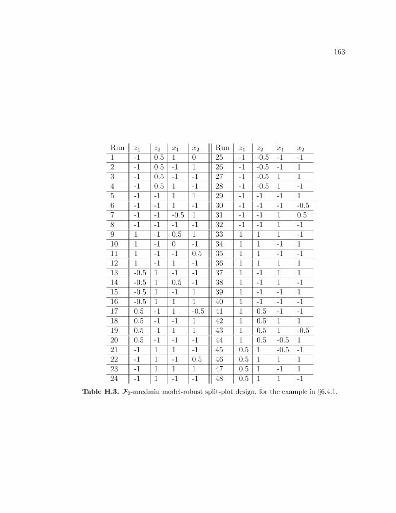
163
Run z1 z2 x1 x2 Run z1 z2 x1 x2
1 -1 0.5 1 0 25 -1 -0.5 -1 -12 -1 0.5 -1 1 26 -1 -0.5 -1 13 -1 0.5 -1 -1 27 -1 -0.5 1 14 -1 0.5 1 -1 28 -1 -0.5 1 -15 -1 -1 1 1 29 -1 -1 -1 16 -1 -1 1 -1 30 -1 -1 -1 -0.57 -1 -1 -0.5 1 31 -1 -1 1 0.58 -1 -1 -1 -1 32 -1 -1 1 -19 1 -1 0.5 1 33 1 1 1 -110 1 -1 0 -1 34 1 1 -1 111 1 -1 -1 0.5 35 1 1 -1 -112 1 -1 1 -1 36 1 1 1 113 -0.5 1 -1 -1 37 1 -1 1 114 -0.5 1 0.5 -1 38 1 -1 1 -115 -0.5 1 -1 1 39 1 -1 -1 116 -0.5 1 1 1 40 1 -1 -1 -117 0.5 -1 1 -0.5 41 1 0.5 -1 -118 0.5 -1 -1 1 42 1 0.5 1 119 0.5 -1 1 1 43 1 0.5 1 -0.520 0.5 -1 -1 -1 44 1 0.5 -0.5 121 -1 1 1 -1 45 0.5 1 -0.5 -122 -1 1 -1 0.5 46 0.5 1 1 123 -1 1 1 1 47 0.5 1 -1 124 -1 1 -1 -1 48 0.5 1 1 -1
Table H.3. F2-maximin model-robust split-plot design, for the example in §6.4.1.

164
Run z1 z2 x1 x2 Run z1 z2 x1 x2
1 -0.5 -1 -1 1 25 1 0 0 02 -0.5 -1 -1 -1 26 1 0 -1 13 -0.5 -1 0 -1 27 1 0 1 -14 -0.5 -1 1 0 28 1 0 1 15 -1 -0.5 -1 0 29 -0.5 1 0 -16 -1 -0.5 0 1 30 -0.5 1 1 17 -1 -0.5 1 -1 31 -0.5 1 1 08 -1 -0.5 1 1 32 -0.5 1 -1 19 -1 0.5 -1 -1 33 0 1 -1 010 -1 0.5 0 1 34 0 1 1 111 -1 0.5 1 -0.5 35 0 1 -1 -112 -1 0.5 -1 1 36 0 1 1 -113 1 -1 -1 -1 37 1 -1 1 114 1 -1 1 -1 38 1 -1 -1 -115 1 -1 1 1 39 1 -1 -1 116 1 -1 -1 1 40 1 -1 1 -117 -1 1 1 -1 41 1 1 -1 -118 -1 1 -1 1 42 1 1 0.5 119 -1 1 -1 -1 43 1 1 -1 120 -1 1 1 1 44 1 1 1 -121 -1 -1 -1 1 45 1 1 -1 -122 -1 -1 1 -1 46 1 1 1 123 -1 -1 1 1 47 1 1 1 -0.524 -1 -1 -1 -1 48 1 1 -1 1
Table H.4. (.8, .8, 1, .5)-F2-maximin model-robust split-plot design, for the example in§6.4.1.

165
Run z1 z2 x1 x2 Run z1 z2 x1 x2
1 -1 -1 -1 -1 25 0 -1 0 02 -1 -1 1 -1 26 0 -1 0 03 -1 -1 -1 1 27 0 -1 0 04 -1 -1 1 1 28 0 -1 0 05 1 -1 -1 -1 29 0 1 0 06 1 -1 1 -1 30 0 1 0 07 1 -1 -1 1 31 0 1 0 08 1 -1 1 1 32 0 1 0 09 -1 1 -1 -1 33 0 -1 010 -1 1 1 -1 34 0 0 1 011 -1 1 -1 1 35 0 0 0 -112 -1 1 1 1 36 0 0 0 113 1 1 -1 -1 37 0 0 0 014 1 1 1 -1 38 0 0 0 015 1 1 -1 1 39 0 0 0 016 1 1 1 1 40 0 0 0 017 -1 0 0 0 41 0 0 0 018 -1 0 0 0 42 0 0 0 019 -1 0 0 0 43 0 0 0 020 -1 0 0 0 44 0 0 0 021 1 0 0 0 45 0 0 0 022 1 0 0 0 46 0 0 0 023 1 0 0 0 47 0 0 0 024 1 0 0 0 48 0 0 0 0
Table H.5. Design used by Vining et al. [103], for the example in §6.4.1.

166
Run z1 z2 x1 x2 Run z1 z2 x1 x2
1 -1 1 1 1 25 -1 -1 -1 12 -1 1 1 -1 26 -1 -1 1 -13 -1 1 -1 -1 27 -1 -1 -1 -14 -1 1 -1 1 28 -1 -1 1 15 1 -1 1 -1 29 -1 1 -1 16 1 -1 1 -1 30 -1 1 1 -17 1 -1 -1 1 31 -1 1 1 -18 1 -1 -1 1 32 -1 1 -1 19 1 1 1 1 33 1 1 1 -110 1 1 -1 -1 34 1 1 -1 -111 1 1 -1 -1 35 1 1 -1 112 1 1 1 1 36 1 1 1 113 1 -1 1 1 37 -1 1 1 -114 1 -1 -1 1 38 -1 1 -1 115 1 -1 1 -1 39 -1 1 1 116 1 -1 -1 -1 40 -1 1 -1 -117 -1 -1 1 1 41 1 1 -1 -118 -1 -1 -1 -1 42 1 1 1 119 -1 -1 -1 -1 43 1 1 -1 120 -1 -1 1 1 44 1 1 1 -121 1 -1 1 -1 45 -1 -1 -1 122 1 -1 1 1 46 -1 -1 -1 -123 1 -1 -1 -1 47 -1 -1 1 124 1 -1 -1 1 48 -1 -1 1 -1
Table H.6. Optimal split-plot design for model (6.9) assuming η = 1, for the examplein §6.4.1.

167
Run z1 z2 x1 x2 Run z1 z2 x1 x2
1 1 1 1 -1 25 -1 -1 -1 -12 1 1 -1 -1 26 -1 -1 -1 13 1 1 1 1 27 -1 -1 1 -14 1 1 -1 1 28 -1 -1 1 15 -1 -1 1 1 29 -1 1 1 16 -1 -1 -1 1 30 -1 1 -1 17 -1 -1 1 -1 31 -1 1 -1 -18 -1 -1 -1 -1 32 -1 1 1 -19 -1 1 1 1 33 1 1 1 -110 -1 1 1 -1 34 1 1 1 111 -1 1 -1 -1 35 1 1 -1 -112 -1 1 -1 1 36 1 1 -1 113 1 -1 -1 1 37 1 -1 1 -114 1 -1 1 1 38 1 -1 -1 -115 1 -1 -1 -1 39 1 -1 1 116 1 -1 1 -1 40 1 -1 -1 117 1 1 -1 1 41 1 -1 -1 -118 1 1 1 1 42 1 -1 -1 119 1 1 1 -1 43 1 -1 1 120 1 1 -1 -1 44 1 -1 1 -121 -1 -1 1 -1 45 -1 1 1 -122 -1 -1 -1 1 46 -1 1 -1 123 -1 -1 -1 -1 47 -1 1 1 124 -1 -1 1 1 48 -1 1 -1 -1
Table H.7. Optimal split-plot design for model (6.10) assuming η = 1, for the examplein §6.4.1.

168
Run z1 z2 x1 x2 Run z1 z2 x1 x2
1 0 -1 -1 0 25 1 1 0 -12 0 -1 -1 1 26 1 1 1 03 0 -1 1 1 27 1 1 -1 -14 0 -1 0 -1 28 1 1 -1 15 -1 0 -1 0 29 -1 1 -1 16 -1 0 1 -1 30 -1 1 -1 -17 -1 0 -1 -1 31 -1 1 1 -18 -1 0 0 1 32 -1 1 19 1 1 -1 -1 33 0 -1 110 1 1 1 -1 34 0 1 0 011 1 1 1 1 35 0 1 1 112 1 1 -1 1 36 0 1 1 -113 1 0 0 1 37 -1 -1 0 -114 1 0 1 -1 38 -1 -1 -1 -115 1 0 -1 0 39 -1 -1 -1 116 1 0 1 1 40 -1 -1 1 017 -1 -1 1 1 41 -1 1 0 018 -1 -1 1 -1 42 -1 1 -1 -119 -1 -1 -1 1 43 -1 1 1 120 -1 -1 -1 -1 44 -1 1 1 -121 1 -1 -1 -1 45 1 -1 1 122 1 -1 0 1 46 1 -1 -1 -123 1 -1 1 -1 47 1 -1 1 -124 1 -1 1 0 48 1 -1 -1 1
Table H.8. Optimal split-plot design for model (6.11) assuming η = 1, for the examplein §6.4.1.

169
Run z1 z2 x1 x2 Run z1 z2 x1 x2
1 0 -1 -0.5 -1 25 0 0 -0.5 12 0 -1 0.5 1 26 0 0 -1 -13 0 -1 -1 1 27 0 0 1 -14 0 -1 1 -0.5 28 0 0 1 15 -1 -1 -0.5 1 29 -1 0 1 -0.56 -1 -1 1 0.5 30 -1 0 -1 17 -1 -1 1 -1 31 -1 0 0.5 18 -1 -1 -1 -0.5 32 -1 0 -0.5 -19 0.5 0.5 -1 1 33 0.5 1 -1 010 0.65 0.17 -1 -0.3 34 0.5 1 1 -111 0.5 0 1 0.5 35 0.5 1 1 012 0.5 0 0 -1 36 0.5 1 0 113 1 -0.5 -1 0 37 1 -1 -0.5 0.514 1 -0.5 -0.5 1 38 1 -1 -1 -115 1 -0.5 0 -1 39 1 -1 1 116 1 -0.5 1 0 40 1 -1 1 -117 -1 -1 1 1 41 -1 1 -1 -118 -1 -1 -1 -1 42 -1 1 1 119 -1 -1 -1 0.5 43 -1 1 1 -120 -1 -1 0.5 -0.5 44 -1 1 -0.5 0.521 1 1 -1 -1 45 1 0.5 -0.5 -0.522 1 1 -1 1 46 1 0.5 0.5 0.523 1 1 0.5 -0.5 47 1 0.5 -1 124 1 1 1 1 48 1 0.5 1 -1
Table H.9. Optimal split-plot design for model (6.12) assuming η = 1, for the examplein §6.4.1.

170
Run z1 z2 x1 x2 Run z1 z2 x1 x2
1 -1 -1 -1 -1 25 -1 -1 -1 12 -1 -1 -1 -1 26 -1 -1 -1 13 -1 -1 1 1 27 -1 -1 1 -14 -1 -1 1 1 28 -1 -1 1 -15 1 1 -1 -1 29 -1 1 -1 16 1 1 1 1 30 -1 1 -1 17 1 1 -1 -1 31 -1 1 1 -18 1 1 1 1 32 -1 1 1 -19 1 -1 -1 1 33 -1 -1 1 110 1 -1 1 -1 34 -1 -1 -1 111 1 -1 1 1 35 -1 -1 -1 -112 1 -1 -1 -1 36 -1 -1 1 -113 1 -1 1 -1 37 1 1 1 114 1 -1 -1 -1 38 1 1 1 -115 1 -1 -1 1 39 1 1 -1 116 1 -1 1 1 40 1 1 -1 -117 -1 1 -1 1 41 -1 1 1 118 -1 1 1 -1 42 -1 1 -1 -119 -1 1 -1 -1 43 -1 1 1 -120 -1 1 1 1 44 -1 1 -1 121 1 1 1 -1 45 1 -1 1 122 1 1 -1 1 46 1 -1 -1 -123 1 1 -1 -1 47 1 -1 1 -124 1 1 1 1 48 1 -1 -1 1
Table H.10. Optimal split-plot design for model (6.9) assuming η = 5.65, for theexample in §6.4.1.

171
Run z1 z2 x1 x2 Run z1 z2 x1 x2
1 1 1 -1 1 25 -1 1 1 12 1 1 1 1 26 -1 1 -1 13 1 1 -1 -1 27 -1 1 1 -14 1 1 1 -1 28 -1 1 -1 -15 1 1 1 1 29 1 -1 -1 -16 1 1 1 -1 30 1 -1 -1 17 1 1 -1 1 31 1 -1 1 18 1 1 -1 -1 32 1 -1 1 -19 1 -1 -1 -1 33 -1 -1 -1 -110 1 -1 -1 1 34 -1 -1 1 111 1 -1 1 -1 35 -1 -1 1 -112 1 -1 1 1 36 -1 -1 -1 113 -1 -1 1 -1 37 -1 1 1 114 -1 -1 -1 -1 38 -1 1 -1 -115 -1 -1 -1 1 39 -1 1 -1 116 -1 -1 1 1 40 -1 1 1 -117 -1 1 1 1 41 -1 -1 1 118 -1 1 1 -1 42 -1 -1 1 -119 -1 1 -1 1 43 -1 -1 -1 120 -1 1 -1 -1 44 -1 -1 -1 -121 1 1 1 -1 45 1 -1 1 -122 1 1 1 1 46 1 -1 1 123 1 1 -1 -1 47 1 -1 -1 124 1 1 -1 1 48 1 -1 -1 -1
Table H.11. Optimal split-plot design for model (6.10) assuming η = 5.65, for theexample in §6.4.1.

172
Run z1 z2 x1 x2 Run z1 z2 x1 x2
1 1 -1 1 1 25 1 -1 -1 -12 1 -1 -1 1 26 1 -1 0 13 1 -1 1 -1 27 1 -1 -1 14 1 -1 -1 -1 28 1 -1 1 05 0 1 1 -1 29 -1 -1 1 16 0 1 0 -1 30 -1 -1 1 -17 0 1 1 1 31 -1 -1 -1 08 0 1 -1 0 32 -1 -1 0 -19 -1 1 1 0 33 1 1 1 110 -1 1 -1 1 34 1 1 1 -111 -1 1 -1 -1 35 1 1 -1 -112 -1 1 0 1 36 1 1 -1 113 -1 -1 1 1 37 1 0 1 114 -1 -1 -1 -1 38 1 0 0 015 -1 -1 -1 1 39 1 0 1 -116 -1 -1 1 -1 40 1 0 -1 -117 -1 0 -1 1 41 -1 1 1 -118 -1 0 1 0 42 -1 1 -1 -119 -1 0 0 1 43 -1 1 -1 120 -1 0 -1 -1 44 -1 1 1 121 0 -1 0 0 45 1 1 -1 -122 0 -1 -1 1 46 1 1 1 123 0 -1 1 -1 47 1 1 1 -124 0 -1 1 1 48 1 1 -1 1
Table H.12. Optimal split-plot design for model (6.11) assuming η = 5.65, for theexample in §6.4.1.
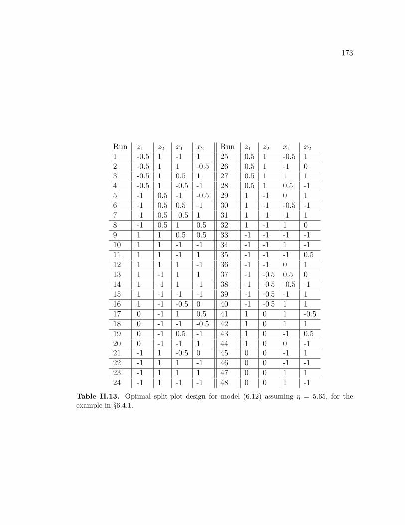
173
Run z1 z2 x1 x2 Run z1 z2 x1 x2
1 -0.5 1 -1 1 25 0.5 1 -0.5 12 -0.5 1 1 -0.5 26 0.5 1 -1 03 -0.5 1 0.5 1 27 0.5 1 1 14 -0.5 1 -0.5 -1 28 0.5 1 0.5 -15 -1 0.5 -1 -0.5 29 1 -1 0 16 -1 0.5 0.5 -1 30 1 -1 -0.5 -17 -1 0.5 -0.5 1 31 1 -1 -1 18 -1 0.5 1 0.5 32 1 -1 1 09 1 1 0.5 0.5 33 -1 -1 -1 -110 1 1 -1 -1 34 -1 -1 1 -111 1 1 -1 1 35 -1 -1 -1 0.512 1 1 1 -1 36 -1 -1 0 113 1 -1 1 1 37 -1 -0.5 0.5 014 1 -1 1 -1 38 -1 -0.5 -0.5 -115 1 -1 -1 -1 39 -1 -0.5 -1 116 1 -1 -0.5 0 40 -1 -0.5 1 117 0 -1 1 0.5 41 1 0 1 -0.518 0 -1 -1 -0.5 42 1 0 1 119 0 -1 0.5 -1 43 1 0 -1 0.520 0 -1 -1 1 44 1 0 0 -121 -1 1 -0.5 0 45 0 0 -1 122 -1 1 1 -1 46 0 0 -1 -123 -1 1 1 1 47 0 0 1 124 -1 1 -1 -1 48 0 0 1 -1
Table H.13. Optimal split-plot design for model (6.12) assuming η = 5.65, for theexample in §6.4.1.

174
H.2 Designs for Example in §6.4.2
Run z1 z2 x1 x2 x3
1 -1 1 0 0 12 -1 1 0.5 0.5 03 -1 1 1 0 04 -1 1 0 1 05 1 -1 1 0 06 1 -1 0.5 0 0.57 1 -1 0 1 08 1 -1 0 0 19 1 1 1 0 010 1 1 0 0.5 0.511 1 1 0.5 0 0.512 1 1 0 1 013 -1 1 0 0.5 0.514 -1 1 1 0 015 -1 1 0 1 016 -1 1 0 0 117 1 1 0.5 0 0.518 1 1 0 1 019 1 1 0 0 120 1 1 1 0 021 -1 -1 0.5 0.5 022 -1 -1 0 0 123 -1 -1 0 1 024 -1 -1 1 0 025 -1 -1 0 1 026 -1 -1 0.5 0.5 027 -1 -1 0 0 128 -1 -1 1 0 0
Table H.14. F1-maximin model-robust design, for the example in §6.4.2.

175
Run z1 z2 x1 x2 x3
1 -1 -1 0 0.5 0.52 -1 -1 0 1 03 -1 -1 0 0 14 -1 -1 1 0 05 1 1 0 1 06 1 1 0 0 17 1 1 1 0 08 1 1 0 0 19 -1 1 0.5 0 0.510 -1 1 0 0 111 -1 1 1 0 012 -1 1 0 1 013 -1 -1 0 1 014 -1 -1 0.5 0.5 015 -1 -1 0 0 116 -1 -1 1 0 017 -1 1 0 0 118 -1 1 0 1 019 -1 1 0 0.5 0.520 -1 1 1 0 021 1 -1 0 0 122 1 -1 1 0 023 1 -1 0.5 0 0.524 1 -1 0 1 025 1 -1 0 0 126 1 -1 0.5 0.5 027 1 -1 0 1 028 1 -1 1 0 0
Table H.15. (.7, .9, 1, 1, 1, 1)-F1-maximin model-robust design, for the example in§6.4.2.

176
Run z1 z2 x1 x2 x3
1 1 1 0 0 12 1 1 1 0 03 1 1 0.5 0 0.54 1 1 0 1 05 -1 1 0.5 0.5 06 -1 1 0 1 07 -1 1 0 0 18 -1 1 1 0 09 1 1 1 0 010 1 1 0 1 011 1 1 0 0.5 0.512 1 1 0 0 113 0 -1 0.5 0.5 014 0 -1 0.5 0 0.515 0 -1 0 1 016 0 -1 0 0 117 1 -1 1 0 018 1 -1 0 1 019 1 -1 1 0 020 1 -1 0 0 121 -1 -1 1 0 022 -1 -1 2/3 1/6 1/623 -1 -1 0 0 124 -1 -1 0 1 025 -1 0 0 0.5 0.526 -1 0 0 0 127 -1 0 1 0 028 -1 0 0 1 0
Table H.16. (1, 1, 1, 1, 1, 1, .5, .5, .5, .5, .5, .5)-F2-maximin design, for the example in§6.4.2.

177
Run z1 z2 x1 x2 x3
1 -1 1 1 0 02 -1 1 0 1 03 -1 1 0 0 14 -1 1 1/3 1/3 1/35 1 -1 1 0 06 1 -1 0 1 07 1 -1 0 0 18 1 -1 1/3 1/3 1/39 1 1 0.5 0.5 010 1 1 0.5 0 0.511 1 1 0 0.5 0.512 1 1 1/3 1/3 1/313 -1 -1 0.5 0.5 014 -1 -1 0.5 0 0.515 -1 -1 0 0.5 0.516 -1 -1 1/3 1/3 1/317 0 0 1/3 1/3 1/318 0 0 1/3 1/3 1/319 0 0 1/3 1/3 1/320 0 0 1/3 1/3 1/321 0 0 1/3 1/3 1/322 0 0 1/3 1/3 1/323 0 0 1/3 1/3 1/324 0 0 1/3 1/3 1/325 0 0 1/3 1/3 1/326 0 0 1/3 1/3 1/327 0 0 1/3 1/3 1/328 0 0 1/3 1/3 1/3
Table H.17. Design from Kowalski et al. [68], for the example in §6.4.2.

178
Run z1 z2 x1 x2 x3
1 1 0 0.5 0.5 02 1 0 0.5 0 0.53 1 0 0 0 14 1 0 0 1 05 1 1 0 0 16 1 1 0 0.5 0.57 1 1 0 1 08 1 1 1 0 09 0 1 0 1 010 0 1 1/3 1/3 1/311 0 1 0 0 112 0 1 1 0 013 -1 -1 0 1 014 -1 -1 0.5 0 0.515 -1 -1 1 0 016 -1 -1 0 0 117 1 -1 0 0.5 0.518 1 -1 0 1 019 1 -1 0 0 120 1 -1 1 0 021 -1 -1 0 1 022 -1 -1 0.5 0.5 023 -1 -1 0 0 124 -1 -1 1 0 025 -1 1 0 0 126 -1 1 0 0.5 0.527 -1 1 1 0 028 -1 1 0 1 0
Table H.18. F2-maximin model-robust design, for the example in §6.4.2.

179
Run z1 z2 x1 x2 x3
1 1 -1 0 0 12 1 -1 0 1 03 1 -1 1 0 04 1 -1 1 0 05 1 1 1 0 06 1 1 1/3 1/3 1/37 1 1 0 1 08 1 1 0 0 19 1 1 0 1 010 1 1 0.5 0 0.511 1 1 1 0 012 1 1 0 0 113 -1 0 0 0.5 0.514 -1 0 0 0 115 -1 0 0 1 016 -1 0 1 0 017 -1 1 0 0.5 0.518 -1 1 0 1 019 -1 1 1 0 020 -1 1 0 0 121 -1 -1 1 0 022 -1 -1 0.5 0.5 023 -1 -1 0 1 024 -1 -1 0 0 125 0 -1 0.5 0 0.526 0 -1 0.5 0.5 027 0 -1 0 1 028 0 -1 0 0 1
Table H.19. (1, 1, 1, 1, 1, 1, .9, .9, .9, .9, .9, .9)-F2-maximin design, for the example in§6.4.2.

180
Run z1 z2 x1 x2 x3
1 1 0 0.5 0 0.52 1 0 1 0 03 1 0 0 0 14 1 0 0 1 05 -1 -1 0 0 16 -1 -1 0 0.5 0.57 -1 -1 1 0 08 -1 -1 0 1 09 -1 1 0 0.5 0.510 -1 1 0 0 111 -1 1 1 0 012 -1 1 0 1 013 -1 -1 0.5 0 0.514 -1 -1 0 1 015 -1 -1 1 0 016 -1 -1 0 0 117 1 1 0 1 018 1 1 1/3 1/3 1/319 1 1 1 0 020 1 1 0 0 121 1 -1 0.5 0.5 022 1 -1 1 0 023 1 -1 0 0 124 1 -1 0 1 025 0 1 1 0 026 0 1 0 1 027 0 1 0.5 0.5 028 0 1 0 0 1
Table H.20. F3-maximin model-robust design, for the example in §6.4.2.

181
Run z1 z2 x1 x2 x3
1 -1 -1 1 0 02 -1 -1 0 0 13 -1 -1 0.5 0 0.54 -1 -1 0 1 05 -1 1 0 1 06 -1 1 0 0.5 0.57 -1 1 0 0 18 -1 1 1 0 09 1 -1 0.5 0 0.510 1 -1 1 0 011 1 -1 0 0 112 1 -1 0 1 013 0 1 0 0.5 0.514 0 1 0.5 0.5 015 0 1 0.5 0 0.516 0 1 0 1 017 1 1 1 0 018 1 1 0 0 119 1 1 1/3 1/3 1/320 1 1 0 1 021 1 0 0.5 0.5 022 1 0 0 0 123 1 0 0 0.5 0.524 1 0 1 0 025 -1 -1 1 0 026 -1 -1 0 0 127 -1 -1 0.5 0.5 028 -1 -1 0 1 0
Table H.21. (.7, 1, .9)-F3-maximin model-robust design, for the example in §6.4.2.

182
Run z1 z2 x1 x2 x3
1 -1 1 0 0 12 -1 1 1 0 03 -1 1 1 0 04 -1 1 0 1 05 0 1 0 0 16 0 1 1 0 07 0 1 0 0 18 0 1 0 1 09 -1 0 1 0 010 -1 0 0 0 111 -1 0 1 0 012 -1 0 0 1 013 -1 0 1 0 014 -1 0 0 0 115 -1 0 0 1 016 -1 0 0 1 017 1 -1 1 0 018 1 -1 1 0 019 1 -1 0 1 020 1 -1 0 0 121 0 1 0 0 122 0 1 0 1 023 0 1 1 0 024 0 1 0 0 125 0 1 0 1 026 0 1 1 0 027 0 1 0 1 028 0 1 0 0 1
Table H.22. Design optimal for model (6.14), for the example in §6.4.2.
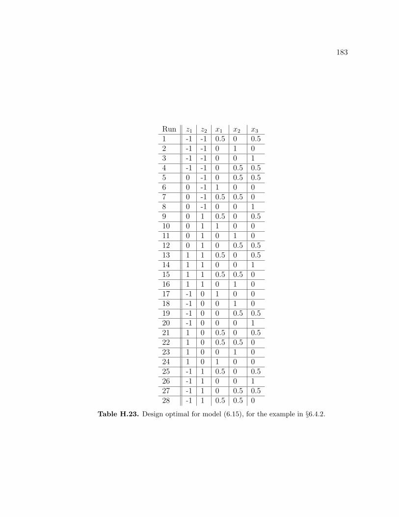
183
Run z1 z2 x1 x2 x3
1 -1 -1 0.5 0 0.52 -1 -1 0 1 03 -1 -1 0 0 14 -1 -1 0 0.5 0.55 0 -1 0 0.5 0.56 0 -1 1 0 07 0 -1 0.5 0.5 08 0 -1 0 0 19 0 1 0.5 0 0.510 0 1 1 0 011 0 1 0 1 012 0 1 0 0.5 0.513 1 1 0.5 0 0.514 1 1 0 0 115 1 1 0.5 0.5 016 1 1 0 1 017 -1 0 1 0 018 -1 0 0 1 019 -1 0 0 0.5 0.520 -1 0 0 0 121 1 0 0.5 0 0.522 1 0 0.5 0.5 023 1 0 0 1 024 1 0 1 0 025 -1 1 0.5 0 0.526 -1 1 0 0 127 -1 1 0 0.5 0.528 -1 1 0.5 0.5 0
Table H.23. Design optimal for model (6.15), for the example in §6.4.2.

184
Run z1 z2 x1 x2 x3
1 1 1 1 0 02 1 1 0 1 03 1 1 0 0 14 1 1 0 0 15 -1 1 0 0 16 -1 1 0 1 07 -1 1 1 0 08 -1 1 0 0 19 1 -1 0 0 110 1 -1 1 0 011 1 -1 0 1 012 1 -1 1 0 013 -1 -1 0 1 014 -1 -1 0 1 015 -1 -1 1 0 016 -1 -1 0 0 117 1 1 0 0 118 1 1 0 1 019 1 1 0 1 020 1 1 1 0 021 -1 1 0 1 022 -1 1 0 0 123 -1 1 1 0 024 -1 1 0 1 025 -1 -1 0 1 026 -1 -1 0 0 127 -1 -1 1 0 028 -1 -1 0 0 1
Table H.24. Design optimal for model (6.16), for the example in §6.4.2.

185
Run z1 z2 x1 x2 x3
1 1 1 0 1 02 1 1 1 0 03 1 1 1 0 04 1 1 0 0 15 -1 1 0 1 06 -1 1 1 0 07 -1 1 0 0 18 -1 1 1 0 09 -1 -1 0 1 010 -1 -1 0 1 011 -1 -1 1 0 012 -1 -1 0 0 113 1 1 0 0 114 1 1 0 0 115 1 1 1 0 016 1 1 0 1 017 1 -1 0 1 018 1 -1 0 0 119 1 -1 1 0 020 1 -1 1 0 021 -1 1 1 0 022 -1 1 0 0 123 -1 1 0 0 124 -1 1 0 1 025 1 -1 0 0 126 1 -1 0 0 127 1 -1 0 1 028 1 -1 1 0 0
Table H.25. Design optimal for model (6.17), for the example in §6.4.2.
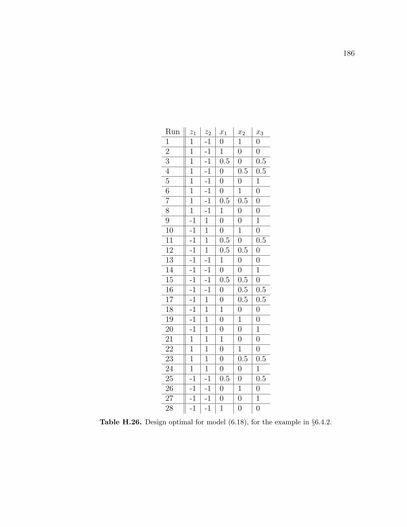
186
Run z1 z2 x1 x2 x3
1 1 -1 0 1 02 1 -1 1 0 03 1 -1 0.5 0 0.54 1 -1 0 0.5 0.55 1 -1 0 0 16 1 -1 0 1 07 1 -1 0.5 0.5 08 1 -1 1 0 09 -1 1 0 0 110 -1 1 0 1 011 -1 1 0.5 0 0.512 -1 1 0.5 0.5 013 -1 -1 1 0 014 -1 -1 0 0 115 -1 -1 0.5 0.5 016 -1 -1 0 0.5 0.517 -1 1 0 0.5 0.518 -1 1 1 0 019 -1 1 0 1 020 -1 1 0 0 121 1 1 1 0 022 1 1 0 1 023 1 1 0 0.5 0.524 1 1 0 0 125 -1 -1 0.5 0 0.526 -1 -1 0 1 027 -1 -1 0 0 128 -1 -1 1 0 0
Table H.26. Design optimal for model (6.18), for the example in §6.4.2.

187
Run z1 z2 x1 x2 x3
1 1 1 0 0 12 1 1 0 1 03 1 1 0 0.5 0.54 1 1 1 0 05 -1 1 1 0 06 -1 1 0.5 0 0.57 -1 1 0 0.5 0.58 -1 1 0 1 09 1 -1 0 0 110 1 -1 0 0.5 0.511 1 -1 0.5 0.5 012 1 -1 1 0 013 1 1 0.5 0 0.514 1 1 0.5 0.5 015 1 1 0 1 016 1 1 0 0 117 -1 1 1 0 018 -1 1 0 0 119 -1 1 0.5 0.5 020 -1 1 0 1 021 1 -1 0 0 122 1 -1 0 1 023 1 -1 0.5 0 0.524 1 -1 1 0 025 -1 -1 0.5 0.5 026 -1 -1 0 1 027 -1 -1 0 0 128 -1 -1 1 0 0
Table H.27. Design optimal for model (6.19), for the example in §6.4.2.

188
Run z1 z2 x1 x2 x3
1 -1 1 0 0.5 0.52 -1 1 1/3 1/3 1/33 -1 1 0 1 04 -1 1 1 0 05 1 1 0 1 06 1 1 1/3 1/3 1/37 1 1 0.5 0 0.58 1 1 0 0 19 -1 1 0 0 110 -1 1 1 0 011 -1 1 0.5 0 0.512 -1 1 0 0.5 0.513 0 1 0 1 014 0 1 1 0 015 0 1 0.5 0.5 016 0 1 0 0 117 -1 0 0.5 0 0.518 -1 0 0.5 0.5 019 -1 0 0 0.5 0.520 -1 0 0 1 021 1 1 0 0 122 1 1 0.5 0.5 023 1 1 0 0.5 0.524 1 1 1/3 1/3 1/325 -1 0 1 0 026 -1 0 0.5 0.5 027 -1 0 0.5 0 0.528 -1 0 1/3 1/3 1/3
Table H.28. Design optimal for model (6.20), for the example in §6.4.2.

189
Run z1 z2 x1 x2 x3
1 1 -1 1 0 02 1 -1 0 0 13 1 -1 0 0 14 1 -1 0 1 05 -1 0 0 0 16 -1 0 0 1 07 -1 0 0 0 18 -1 0 1 0 09 1 1 1 0 010 1 1 0 0 111 1 1 0 0 112 1 1 0 1 013 1 0 0 1 014 1 0 0 0 115 1 0 1 0 016 1 0 0 1 017 0 -1 0 1 018 0 -1 1 0 019 0 -1 1 0 020 0 -1 0 0 121 -1 1 1 0 022 -1 1 0 1 023 -1 1 1 0 024 -1 1 0 0 125 -1 -1 0 0 126 -1 -1 0 1 027 -1 -1 1 0 028 -1 -1 0 1 0
Table H.29. Design optimal for model (6.21), for the example in §6.4.2.

190
Run z1 z2 x1 x2 x3
1 -1 -1 1 0 02 -1 -1 0 1 03 -1 -1 0.5 0 0.54 -1 -1 0 0.5 0.55 1 -1 0 0 16 1 -1 0 1 07 1 -1 0.5 0.5 08 1 -1 0.5 0 0.59 1 -1 0 0 110 1 -1 0 1 011 1 -1 1/3 1/3 1/312 1 -1 1 0 013 1 1 1 0 014 1 1 0 0.5 0.515 1 1 0 1 016 1 1 0 0 117 -1 1 1/3 1/3 1/318 -1 1 0 0 119 -1 1 0 1 020 -1 1 1 0 021 -1 -1 1 0 022 -1 -1 0 1 023 -1 -1 0 0 124 -1 -1 0.5 0.5 025 -1 1 0 0.5 0.526 -1 1 1/3 1/3 1/327 -1 1 0.5 0.5 028 -1 1 0.5 0 0.5
Table H.30. Design optimal for model (6.22), for the example in §6.4.2.

191
Run z1 z2 x1 x2 x3
1 -1 1 0.5 0 0.52 -1 1 0 1 03 -1 1 1 0 04 -1 1 0 0.5 0.55 1 1 1 0 06 1 1 0 0 17 1 1 0.5 0.5 08 1 1 0 0.5 0.59 1 1 0.5 0 0.510 1 1 0 1 011 1 1 0 0 112 1 1 1 0 013 -1 1 0 1 014 -1 1 0 0 115 -1 1 1 0 016 -1 1 0.5 0.5 017 -1 -1 1 0 018 -1 -1 1/3 1/3 1/319 -1 -1 0 1 020 -1 -1 0 0 121 1 -1 0 1 022 1 -1 1 0 023 1 -1 0 0 124 1 -1 1/3 1/3 1/325 -1 -1 0.5 0 0.526 -1 -1 0 0.5 0.527 -1 -1 0.5 0.5 028 -1 -1 1/3 1/3 1/3
Table H.31. Design optimal for model (6.23), for the example in §6.4.2.

192
Run z1 z2 x1 x2 x3
1 1 -1 1 0 02 1 -1 0 0 13 1 -1 0 1 04 1 -1 0.5 0 0.55 1 0 0 1 06 1 0 0.5 0 0.57 1 0 0 0 18 1 0 0.5 0.5 09 -1 -1 1 0 010 -1 -1 0 1 011 -1 -1 0.5 0 0.512 -1 -1 0 0 113 1 1 0 1 014 1 1 0 0.5 0.515 1 1 0 0 116 1 1 1 0 017 -1 1 1 0 018 -1 1 0 1 019 -1 1 0 0 120 -1 1 0.5 0.5 021 0 1 0.5 0 0.522 0 1 0 1 023 0 1 0 0.5 0.524 0 1 1 0 025 0 -1 1 0 026 0 -1 0 0.5 0.527 0 -1 0.5 0.5 028 0 -1 0 0 1
Table H.32. Design optimal for model (6.24), for the example in §6.4.2.
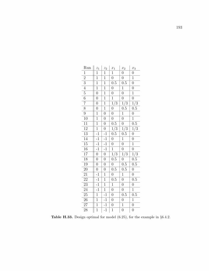
193
Run z1 z2 x1 x2 x3
1 1 1 1 0 02 1 1 0 0 13 1 1 0.5 0.5 04 1 1 0 1 05 0 1 0 0 16 0 1 1 0 07 0 1 1/3 1/3 1/38 0 1 0 0.5 0.59 1 0 0 1 010 1 0 0 0 111 1 0 0.5 0 0.512 1 0 1/3 1/3 1/313 -1 -1 0.5 0.5 014 -1 -1 0 1 015 -1 -1 0 0 116 -1 -1 1 0 017 0 0 1/3 1/3 1/318 0 0 0.5 0 0.519 0 0 0 0.5 0.520 0 0 0.5 0.5 021 -1 1 0 1 022 -1 1 0.5 0 0.523 -1 1 1 0 024 -1 1 0 0 125 1 -1 0 0.5 0.526 1 -1 0 0 127 1 -1 0 1 028 1 -1 1 0 0
Table H.33. Design optimal for model (6.25), for the example in §6.4.2.

Bibliography
[1] V. K. Agboto and C. J. Nachtsheim. Bayesian model robust designs. Tech-nical report, University of Minnesota, 2005.
[2] F. T. Anbari and J. M. Lucas. Super-efficient designs: How to run your ex-periment for higher efficiency and lower cost. In ASQC 48th Annual QualityCongress Proceedings, 1994.
[3] F. T. Anbari and J. M. Lucas. Design and running super-efficient experi-ments: Optimum blocking with one hard-to-change factor. Journal of QualityTechnology, 40(1):31–45, 2008.
[4] T. W. Anderson. An Introduction to Multivariate Statistical Analysis. NewYork: Wiley, 1984.
[5] H. Arnouts and P. Goos. Update formulas for split-plot and block designs.Technical Report 2008-022, University of Antwerp, Faculty of Applied Eco-nomics, Department of Mathematics, Statistics, and Actuarial Sciences, De-cember 2008.
[6] H. Arnouts, P. Goos, and B. Jones. Design and analysis of industrial strip-plot experiments. Quality and Reliability Engineering International, 26:127–136, 2010.
[7] S. P. Aspery and S. Macchietto. Designing robust optimal dynamic experi-ments. Journal of Process Control, 12(4):545–556, 2002.
[8] A. B. Atashgah and A. Seifi. Application of semi-definite programming tothe design of multi-response experiments. IIE Transactions, 39:7:763–769,2007.
[9] A. B. Atashgah and A. Seifi. Optimal design of multi-response experimentsusing semi-definite programming. Optimization and Engineering, 10(1):75–90, 2009.

195
[10] A. C. Atkinson, A. N. Donev, and R. D. Tobias. Optimum ExperimentalDesigns, with SAS. Oxford University Press, 2007.
[11] M. P. F. Berger and F. E. S. Tan. Robust designs for linear mixed effectsmodels. Journal of the Royal Statistical Society: Series C (Applied Statis-tics), 53(4):569–581, 2004.
[12] D. Bingham and R. R. Sitter. Minimum-aberration two-level fractional fac-torial split-plot designs. Technometrics, 41(1):62–70, 1999.
[13] D. R. Bingham and H. A. Chipman. Incorporating prior information inoptimal design for model selection. Technometrics, 49(2):155–163, 2007.
[14] D. R. Bingham and R. R. Sitter. Design issues in fractional factorial split-plotexperiments. Journal of Quality Technology, 33(1):2–15, 2001.
[15] W. Bischoff. On d-optimal designs for linear models under correlated obser-vations with an application to a linear model with multiple response. Journalof Statistical Planning and Inference, 37:69–80, 1993.
[16] W. Bischoff. Determinant formulas with applications to designing when theobservations are correlated. Annals of the Institute of Statistical Mathemat-ics, 47(2):385–399, 1995.
[17] S. Bisgaard. The design and analysis of 2k−p × 2q−r split plot experiments.Journal of Quality Technology, 32(1):39–56, 2000.
[18] G. E. P. Box and N. R. Draper. A basis for the selection of a response surfacedesign. Journal of the American Statistical Association, 54(287):622–654,1959.
[19] G. E. P. Box and N. R. Draper. The bayesian estimation of common param-eters from several responses. Biometrika, 52(3/4):355–365, 1965.
[20] M. J. Box and N. R. Draper. Estimation and design criteria for multire-sponse non-linear models with non-homogenous variance. Applied Statistics,21(1):13–24, 1972.
[21] F. Chang, M. L. Huang, D. K. J. Lin, and H. Yang. Optimal designs fordual response polynomial regression models. Journal of Statistical Planningand Inference, 93:309–322, 2001.
[22] S. I. Chang. Some properties of multi-response d-optimal designs. Journalof Mathematical Analysis and Applications, 184:256–262, 1994.
[23] S. I. Chang. An algorithm to generate near d-optimal designs for multiple-response surface models. IIE Transactions, 29:1073–1081, 1997.

196
[24] Y.-J. Chang and W. I. Notz. Handbook of Statistics, Vol. 13, chapter ModelRobust Designs, pages 1055–1098. Elsevier Science B. V., 1996.
[25] H. Chipman, M. Hamada, and C. F. J. Wu. A bayesian variable selectionapproach for analyzing designed experiments with complex aliasing. Tech-nometrics, 39:372–381, 1997.
[26] R. D. Cook and C. J. Nachtsheim. A comparison of algorithms for construct-ing exact d-optimal designs. Technometrics, 22:315–324, 1980.
[27] R. D. Cook and C. J. Nachtsheim. An analysis of the k-exchange algorithm.Technical report, University of Minnesota, Dept. of Operations and Manage-ment Science, 1982.
[28] R. D. Cook and C. J. Nachtsheim. Model-robust, linear-optimal designs.Technometrics, 24:49–54, 1982.
[29] J. Cornell. Experiments with Mixtures: Designs, Models, and the Analysisof Mixture Data. Wiley-Interscience, 2nd edition, s 1990.
[30] C. Daniel. Parallel fractional replicates. Technometrics, 2(2):263–268, 1960.
[31] H. Dette. A generalization of D- and D1-optimal design in polynomial re-gression. Annals of Statistics, 18:1784–1804, 1990.
[32] H. Dette and T. Franke. Constrained d- and d1-optimal designs for polyno-mial regression. The Annals of Statistics, 28(6):1702–1727, 2000.
[33] H. Dette and T. Franke. Robust designs for polynomial regression by max-imizing a minimum of D- and D1-efficiencies. The Annals of Statistics,29(4):1024–1049, 2001.
[34] N. R. Draper and W. G. Hunter. Design of experiments for parameter esti-mation in multiresponse situations. Biometrika, 53:525–533, 1966.
[35] N. R. Draper and W. G. Hunter. The use of prior distributions in the design ofexperiments for parameter estimation in non-linear situations: Multiresponsecase. Biometrika, 54(3/4):662–665, 1967.
[36] N. R. Draper and J. A. John. Response surface designs where levels ofsome factors are difficult to change. Australian and New Zealand Journal ofStatistics, 40(4):487–495, 1998.
[37] W. DuMouchel and B. Jones. A simple bayesian modification of d-optimal de-signs to reduce dependence on an assumed model. Technometrics, 36(1):37–47, 1994.

197
[38] M. Emmett, P. Goos, and E. Stillman. D-optimal designs for multiple poly-nomial responses. Technical report, University of Sheffield, 2007.
[39] Z. Fang and D. P. Wiens. Integer-valued, minimax robust designs for es-timation and extrapolation in heteroscedastic, approximate linear models.Journal of the American Statistical Association, 95(451):807–818, 2000.
[40] Z. Fang and D. P. Wiens. Robust regression designs for approximate poly-nomial models. Journal of Statistical Planning and Inference, 117:305–321,2003.
[41] V. V. Fedorov. Theory of Optimal Experiments. Academic Press, New York,NY, 1972.
[42] S. E. Frisbee and J. W. McGinity. Influence of nonionic surfactants on thephysical and chemical properties of a biodegradable pseudolatex. EuropeanJournal of Pharmaceutics and Biopharmaceutics, 40:355–363, 1994.
[43] J. Ganju and J. M. Lucas. Detecting randomization restrictions caused byfactors. Journal of Statistical Planning and Inference, 81:129–140, 1999.
[44] J. Ganju and J. M. Lucas. Randomized and random run order experiments.Journal of Statistical Planning and Inference, 133:199–210, 2004.
[45] P. Goos. The Optimal Design of Blocked and Split-plot Experiments.Springer, 2002.
[46] P. Goos. Optimal versus orthogonal and equivalent-estimation design ofblocked and split-plot experiments. Statistica Neerlandica, 60:361–378, 2006.
[47] P. Goos and A. N. Donev. Tailor-made split-plot designs for mixture andprocess variables. Journal of Quality Technology, 39(4):326–339, 2007.
[48] P. Goos, A. Kobilinsky, T. E. O’Brien, and M. Vandebroek. Model-robustand model-sensitive designs. Computational Statistics & Data Analysis,49:201–216, 2005.
[49] P. Goos and M. Vandebroek. Optimal split-plot designs. The Journal ofQuality Technology, 33(4):436–450, 2001.
[50] P. Goos and M. Vandebroek. D-optimal split-plot designs with given numbersand sizes of whole plots. Technometrics, 45(3):235–245, 2003.
[51] P. Goos and M. Vandebroek. Outperforming completely randomized designs.Journal of Quality Technology, 36(1):12–26, 2004.

198
[52] J. A. Heinsman and D. C. Montgomery. Optimization of a household productformulation using a mixture experiment. Quality Engineering, 7:583–600,1995.
[53] G. Heo, B. Schmuland, and D. P. Wiens. Restricted minimax robust de-signs for misspecified regression models. The Canadian Journal of Statistics,29(1):117–128, 2001.
[54] A. Heredia-Langner, D. C. Montgomery, W. M. Carlyle, and C. M. Borror.Model-robust optimal designs: A genetic algorithm approach. Journal ofQuality Technology, 36(3):263–279, 2004.
[55] P. Huang, D. Chen, and J. O. Voelkel. Minimum-aberration two-level split-plot designs. Technometrics, 40(4):314–326, 1998.
[56] H. M. Huizenga, D. J. Heslenfeld, and P. C. M. Molenaar. Optimal measure-ment conditions for spatiotemporal eeg/meg source analysis. Psychometrika,67(2):299–313, 2002.
[57] L. Imhof and W. K. Wong. A graphical method for finding maximin efficiencydesigns. Biometrics, 56(1):113–117, 2000.
[58] M. E. Johnson and C. J. Nachtsheim. Some guidelines for constructing exactd-optimal designs on convex design spaces. Technometrics, 25:271–277, 1983.
[59] B. Jones and P. Goos. A candidate-set-free algorithm for generating d-optimal split-plot designs. Journal of the Royal Statistical Society, SeriesC: Applied Statistics, 56:347–364, 2007.
[60] B. Jones and P. Goos. D-optimal design of split-split-plot experiments.Biometrika, 96(1):67–82, 2009.
[61] B. Jones and C. J. Nachtsheim. Split-plot designs: What, why, and how.Journal of Quality Technology, 41(4):340–361, 2009.
[62] H. L. Ju and J. M. Lucas. lk factorial experiments with hard-to-change andeasy-to-change factors. Journal of Quality Technology, 34(4):411–421, 2002.
[63] A. I. Khuri and J. A. Cornell. Response Surfaces: Designs and Analyses. M.Dekker, 1996.
[64] J. Kiefer. Optimum experimental designs. Journal of the Royal StatisticalSociety, Series B, 21:272–304, 1959.
[65] J. Kiefer and J. Wolfowitz. Optimum designs in regression problems. Annalsof Mathematical Statistics, 30:271–294, 1959.

199
[66] J. Kiefer and J. Wolfowitz. The equivalence of two extremum problems.Canadian Journal of Mathematics, 12:363–366, 1960.
[67] W. B. Kim and N. R. Draper. Choosing a design for straight line fits to twocorrelated responses. Statistica Sinica, 4:275–280, 1994.
[68] S. M. Kowalski, J. A. Cornell, and G. G. Vining. Split-plot designs andestimation methods for mixture experiments with process variables. Tech-nometrics, 44(1):72–79, 2002.
[69] O. Krafft and M. Schaefer. D-optimal designs for a multivariate regressionmodel. Journal of Multivariate Analysis, 42:130–140, 1992.
[70] V. G. Kurotschka and R. Schwabe. Madan Puri Festschrift, chapter TheReduction of Design Problems for Multivariate Experiments to UnivariatePossibilities and their Limitations, pages 193–204. VSP, 1996.
[71] E. Lauter. Experimental design in a class of models. Statistics, 5:379–398,1974.
[72] J. D. Letsinger, R. H. Myers, and M. Lentner. Response surface methods forbi-randomization structures. Journal of Quality Technology, 28:4:381–397,1996.
[73] W. Li and C. J. Nachtsheim. Model-robust factorial designs. Technometrics,42(4):345–352, 2000.
[74] S. X. Liu and D. P. Wiens. Robust designs for approximate polynomialregression. Journal of Statistical Planning and Inferences, 64:369–381, 1997.
[75] X. Liu and R. X. Yue. P-optimal robust designs for multiresponse approxi-mately linear regression. Applied Mathematics - A Journal of Chinese Uni-versities, 23(2):168–174, 2008.
[76] J. M. Lucas and H. L. Ju. Split plotting and randomization in industrialexperiments. In ASQC Quality Congress Transactions, 1992.
[77] R. K. Meyer and C. J. Nachtsheim. The coordinate-exchange algorithm forconstructing exact optimal experimental designs. Technometrics, 37(1):60–69, 1995.
[78] K. S. Miller. On the inverse of the sum of matrices. Mathematics Magazine,54(2):67–72, 1981.
[79] T. J. Mitchell. An algorithm for the construction of d-optimal experimentaldesigns. Technometrics, 16:203–210, 1974.

200
[80] G. Montepiedra and V. V. Fedorov. Minimum bias designs with constraints.Journal of Statistical Planning and Inference, 63:97–111, 1997.
[81] G. Montepiedra and A. B. Yeh. A two-stage strategy for the construction ofd-optimal experimental designs. Communications in Statistics - Simulationand Computations, 27(2):377–401, 1998.
[82] D. C. Montgomery. Design and Analysis of Experiments. John Wiley &Sons, Inc., 1991.
[83] A. Neff. Bayesian two-stage designs under model uncertainty. PhD thesis,Virginia Polytechnic Institute and State University, 1996.
[84] P. A. Parker, S. M. Kowalski, and G. G. Vining. Construction of bal-anced equivalent estimation second-order split-plot designs. Technometrics,49(1):56–65, 2007.
[85] G. F. Piepel. Programs for generating extreme vertices and centroids oflinearly constrained experimental regions. Journal of Quality Technology,20:2:125–139, 1988.
[86] G. F. Piepel, S. K. Cooley, and B. Jones. Construction of a 21-componentlayered mixture experiment design using a new mixture coordinate-exchangealgorithm. Quality Engineering, 17:579–594, 2005.
[87] F. Pukelsheim. Optimal Design of Experiments. John Wiley & Sons, Inc.,1993.
[88] F. Pukelsheim and J. L. Rosenberger. Experimental designs for model dis-crimination. Journal of the American Statistical Association, 88(422):642–649, 1993.
[89] R. Rajagopal and E. del Castillo. Model-robust process optimization usingbayesian model averaging. Technometrics, 47(2):152–163, 2005.
[90] R. G. Roy, S. N. and J. N. Srivastava. Analysis and Design of CertainQuantitative Multiresponse Experiments. Pergamon Press, New York, NY,1971.
[91] A. Ruggoo and M. Vandebroek. Bayesian sequential D-D optimal model-robust designs. Computational Statistics & Data Analysis, 47:655–673, 2004.
[92] SAS. SAS Institute Inc., Version 9.1.3, Cary, NC, USA, 2000-2004.
[93] J. R. Schott. Matrix Analysis for Statistics. John Wiley & Sons, Inc., 1997.

201
[94] H. K. Shah, D. C. Montgomery, and W. M. Carlyle. Response surface model-ing and optimization in multiresponse experiments using seemingly unrelatedregressions. Quality Engineering, 16(3):387–397, 2004.
[95] B. J. Smucker, E. del Castillo, and J. L. Rosenberger. Exchange algorithmsfor constructing model-robust experimental designs. Technical Report 09-04,The Pennsylvania State University, 2009.
[96] R. D. Snee. Computer-aided design of experiments–some practical experi-ences. Journal of Quality Technology, 17:222–236, 1985.
[97] S. M. Stigler. Optimal experimental design for polynomial regression. Journalof the American Statistical Association, 66(334):311–318, 1971.
[98] D. X. Sun. Estimation capacity and related topics in experimental designs.PhD thesis, University of Waterloo, 1993.
[99] L. A. Trinca and S. G. Gilmour. Multistratum response surface designs.Technometrics, 43(1):25–33, 2001.
[100] P.-W. Tsai and S. G. Gilmour. A general criterion for factorial designs undermodel uncertainty. Technometrics (to appear), 2010.
[101] C. L. Tseo, J. C. Deng, J. A. Cornell, A. I. Khuri, and R. H. Schmidt. Effectof washing treatment on quality of minced mullet flesh. Journal of FoodScience, 48:163–167, 1983.
[102] G. G. Vining and S. M. Kowalski. Exact inference for response surface designswithin a split-plot structure. Journal of Quality Technology, 40(4):394–406,2008.
[103] G. G. Vining, S. M. Kowalski, and D. C. Montgomery. Response surface de-signs within a split-plot structure. Journal of Quality Technology, 37(2):115–129, 2005.
[104] D. F. Webb, J. M. Lucas, and J. J. Borkowski. Factorial experiments whenfactor levels are not necessarily reset. Journal of Quality Technology, 36(1):1–11, 2004.
[105] W. J. Welch. A mean squared error criterion for the design of experiments.Biometrika, 70(1):205–213, 1983.
[106] D. P. Wiens. Robust minimax designs for multiple linear regression. LinearAlgebra Applications, 127:327–340, 1990.
[107] D. P. Wiens. Minimax designs for approximately linear regression. Journalof Statistical Planning and Inference, 31(3):353–371, 1992.

202
[108] D. P. Wiens. Robust designs for approximately linear regression: M-estimated parameters. Journal of Statistical Planning and Inference,40(1):135–160, 1994.
[109] D. P. Wiens. Minimax robust designs and weights for approximately speci-fied regression models with heteroscedastic errors. Journal of the AmericanStatistical Association, 93:1440–1450, 1998.
[110] D. P. Wiens. Robust weights and designs for biased regression models: Leastsquares and generalized m-estimation. Journal of Statistical Planning andInference, 83(2):395–412, 2000.
[111] D. P. Wiens and J. Zhou. Minimax regression designs for approximatelylinear models with autocorrelated errors. Journal of Statistical Planning andInference, 55(1):95–106, 1996.
[112] M. M. C. Wijesinha. Design of experiments for multiresponse models. PhDthesis, University of Florida, 1984.
[113] F. Yates. Complex experiments, with discussion. Journal of the Royal Sta-tistical Society, Series B, 2:181–223, 1935.
[114] R. X. Yue. Model-robust designs in multiresponse situations. Statistics &Probability Letters, 58:369–379, 2002.
[115] A. Zellner. An efficient method of estimating seemingly unrelated regres-sions and tests for aggregation bias. Journal of the American StatisticalAssociation, 57:348–368, 1962.
[116] A. Zellner. Estimators for seemingly unrelated regression equations: Someexact finite sample results. Journal of the American Statistical Association,58:977–992, 1963.
[117] A. Zellner and D. S. Huang. Further properties of efficient estimators forseemingly unrelated regression equations. International Economic Review,3:300–313, 1962.

Vita
Byran J. Smucker
Byran Jay Smucker was born in Albany, OR on July 13, 1982. He graduatedfrom Brownsville Mennonite School in 1999, attended Linn-Benton CommunityCollege, and graduated summa cum laude from Oregon State University in 2005with a B.S. in Industrial Engineering. In August, 2005 he entered the Departmentof Statistics at The Pennsylvania State University, acquired an M.S. in Statisticsand Operations Research in 2007, and will graduate in August, 2010 with a Ph.Din Statistics and Operations Research. The same month, he will begin an assistantprofessor position in the Statistics Department at Miami University at Oxford, OH.Mr. Smucker is the son of Steve and Bonnie Smucker, with five siblings (Randy,Jessica, Justin, Stephanie, and Trevin). He is married to Amy Smucker, with ason Xavier.