Available online at www.sciencedirect.com

SCIENCE@DIRECT 8 AGRICULTURAL ECONOMICS

ELSEVIER, Agricultural Economics 28 (2003) 197-213 www.elsevier.com/locate/agecon

The impact of farm credit in Pakistan

Shahidur R. Khandker*, Rashid R. Faruqee1

The World Bank, 1818 H Street NW Washington, DC 20433, USA

Received 9 April2001; received in revised form 13 February 2002; accepted 22 July 2002

Abstract

Both informal and formal loans matter in agriculture. However, formal lenders provide many more production loans than informal lenders, often at a cost (mostly loan default cost) higher than what they can recover. For example, the Agricultural Development Bank of Pakistan (ADBP), providing about 90% of formal loans in rural areas, incurs high loan default costs. Yet, like other governments, the Government of Pakistan supports the formal scheme on the grounds that lending to agriculture is a high risk activity because of covariate risk. Hence, such policies are often based on a market failure argument. As farm credit schemes are subsidised, policy makers must know if these schemes are worth supporting. Using a recent large household survey data from rural Pakistan (Rural Financial Market Studies or RFMS), we have attempted to estimate the effectiveness of the ADBP as a credit delivery institution. A two-stage method that takes the endogeneity of borrowing into account is used to estimate credit impact. Results reveal that ADBP contributes to household welfare and that its impact is higher for smallholders than for large holders. Nevertheless, large holders receive the bulk of ADBP finance. The ADBP is, thus, not a cost-effective institution in delivering rural finance. Its cost-effectiveness can be improved by reducing its loan default cost and partially by targeting smallholders in agriculture where credit yields better results. © 2003 Elsevier Science B. V. All rights reserved.

JEL classification: Ql4

Keywords: Agricultural credit; Rural financial institutions; Impact of credit on income and productivity; Cost-effectiveness of credit delivery system

1. Introduction

Credit is important for development. It capitalises farmers and entrepreneurs to undertake new invest­ments or adopt new technologies. It helps smooth consumption by providing working capital and re­duces poverty in the process. Both formal and informal lenders are active in rural credit market (Adams and

* Corresponding author. E-mail address: skhandker@worldbank.org (S.R. Khandker).

1 Shahidur R. Khandker is a Lead Economist at the World Bank and Rashid R. Faruqee was a Lead Economist at the World Bank when the article was written.

Fitchett, 1992; Aleem, 1990; Ghate, 1992; Hussain and Demaine, 1992; Udry, 1990). Collateral-free lend­ing, proximity, timely delivery and flexibility in loan transactions are some of the attractive features of infor­mal credit.2 However, informal finance may not be as conducive to development as formal finance because:

2 Although the nominal rate of interest is lower for formal loans than for informal loans, the transaction costs of borrowing are higher for formal loans than for informal loans. Some informal lenders also perform an important role by facilitating the marketing of products or purchasing of inputs, such as fertiliser. Additionally, since informal loans are often given in kind and for specific purposes, some client needs are served better by informal than by formal loans.

0169-5150/03/$ - see front matter © 2003 Elsevier Science B.V. All rights reserved. doi: 10.1016/S0169-5150(03)00017-3

198 S.R. Khandker, R.R. Faruqee/Agricultural Economics 28 (2003) 197-213

(i) it is expensive;3 (ii) it is short-term and largely used for consumption; and (iii) it is not generally large enough to spur investment and growth.

Notwithstanding the limitations of informal finance, many governments have attempted in the past to de­velop alternative financial institutions to provide credit to farmers and other rural producers. Many such at­tempts have failed not only in delivering credit to tar­get households but also in promoting a viable credit delivery system. High covariate risk of agricultural production (Binswanger and Rosenzweig, 1986), the asymmetric information, lack of enforcement of loan contracts (Hoff and Stiglitz, 1990),4 government im­prudent interference in credit markets, and rent-seeking as a result of credit rationing (Braverman and Guasch, 1989) are some of the factors alleged to be responsible for the poor performance of the government-directed credit schemes in many countries.

With the dismal picture of state-owned rural finance organisations, non-governmental micro-finance insti­tutions have been growing to meet the credit needs of small producers in many countries. Reports indicate that they now meet the credit demand of 10-12 mil­lion people in Africa, Asia and Latin America. 5 Many of these organisations are subsidised not for absorb­ing high loan default costs but for covering high trans­action costs associated with group-based lending and other social intermediation costs (Khandker, 1988). If agricultural credit and other targeted schemes are to be supported, policy makers must know how much they are subsidised, who receives this subsidy, and whether it helps the borrowers.

Assessing the net contribution of a program means evaluating both its costs and benefits. Assessing the costs of lending involves the imputed market cost of the subsidy these schemes receive from the govern­ment and donors. Assessing benefits is often problem­atic because funds are fungible and it is not clear if

3 Some studies, however, question the excessive interest rates of informal lenders (e.g. Hussain and Demaine, 1992).

4 To reduce the moral hazard problem and associated transac­tion costs of lending, financial institutions often ask for physical collateral. Collateral restrictions exclude the poor who do not have assets, such as land, to offer as collateral but are otherwise good credit risks.

5 For a discussion of a broad range of programs, see Otero and Rhyne (1994), Christen et al. (1994), Brugger and Rajpatirana (1995), and Hulme and Mosley (1996).

the measured credit effect reflects the borrowing con­straint or the unobservable characteristics of a bor­rower. The presence of bias caused by self-selection of borrowers into credit programs may bias assessment of benefits of these programs by as much as 100%.6

Nonetheless, there are a number of studies that have successfully estimated program benefits (Binswanger and Khandker, 1995; Carter, 1988; Carter and Weihe, 1990; Feder et al., 1990; Pitt and Khandker, 1996, 1998). Binswanger and Khandker (1995) estimated the impact of formal credit using district-level panel data from India and found that formal credit increases ru­ral income and productivity, and that benefits exceed the cost of the formal system by at least 13%. Feder et al. (1990) estimated a switching regression model for households in China and distinguished between households that are credit-constrained and those that are not.

Pitt and Khandker (1998) examined the impact of credit from the Grameen Bank and other two tar­geted credit programs in Bangladesh on a variety of individual and household outcomes, including school enrolment, labour supply, asset holding, fertility and contraceptive use. They found credit to be a significant determinant of many household outcomes, and that program credit has a significant effect on the well-being of poor households in Bangladesh. Khandker (1988) observed that micro-credit programs are as cost-effective as other programs, such as the food for work, in benefiting the poor.

The objective of this paper is to analyse the role of the Agricultural Development Bank of Pakistan (ADBP) in rural areas and assess its cost-effectiveness in delivering farm credit. The paper's contribu­tion lies in adding to the existing literature on the cost-effectiveness of a government-supported farm credit program which has not been managed well for years. The data used in this paper's analysis are drawn from the Rural Financial Market Studies (RFMS) of Pakistan. Results suggest that the effect of ADBP finance is substantial, and that the impact is higher for smallholders than for medium and large holders in agriculture. But, given the distribution of loans and loan recovery rates, ADBPs lending pro­gram is not cost-effective. The program can be made cost-effective by supporting smallholders (who own

6 See McKernan (1996).

S.R. Khandker, R.R. Faruqee/ Agricultural Economics 28 (2003) 197-213 199

up to 2.5 acres of land) more than medium and large holders, by improving both loan recovery and admin­istrative efficiency, and by making operations liable to a lending portfolio.?

The paper is organised as follows. Section 2 de­scribes the survey and sample data used for the study. Section 3 describes the rural credit market in Pak­istan. A number of studies including recent data show that the market share of institutional credit is low de­spite government intervention since 1960. Also, for­mal credit has failed to reach the borrowers who may be able to use credit more productively. Section 4 ex­plains the econometric model used to asses the credit impacts on different household outcomes. Section 5 discusses the regression results. Based on two-stage estimation techniques, formal credit is found to have significant positive impacts on most household out­comes considered in this paper. Section 6 shows how much social costs are involved for ADBP in provid­ing credit. Section 7 presents the cost-benefit analysis of the ADBP. The concluding section summarises the findings and discusses policy options.

2. Data

Data from the RFMS, collected for the State Bank of Pakistan with financial assistance from the World Bank in 1996, are used. Household survey and in­formal lenders' survey data were collected by two organisations: (1) the Applied Economic Research Centre (AERC, 1998) of the University of Karachi and (2) the Punjab Economic Research Institute (PERI) in Lahore. The Pakistan Institute of Devel­opment Economics (PIDE) in Islamabad collected the institutional data on the ADBP and commercial banks working in the rural sector. Household survey data were collected for all five provinces of Pakistan, namely, north western frontier province (NWFP), Sindh, Balochistan, Punjab and Pakistan controlled Kashmir (AJ&K). A rural household survey was conducted on the pattern of the LSMS surveys con­ducted by the World Bank to provide the data base.

7 By providing more loans to smallholders, transaction costs may increase but loan default costs will decrease, because the loan recovery rates are higher for smallholders than for large holders in agriculture.

The survey covered various aspects of the household economy, including demographic information, labour supply, household expenditure, income sources, farm production, borrowing practices, assets and liabilities.

A two-stage stratified sampling strategy was adopted for selection of villages and households. In the first stage, 250 villages were selected randomly from a total of approximately 50,000 villages in Pakistan (as reported in Agricultural Statistics, 1994-1995). The allocation of villages within the provinces was done in proportion to cultivated area. A completely randomised sampling strategy was adopted for each provincial sample. Villages were selected randomly from the province after excluding very small and very large villages, depending on the size distribution of villages within each province.

In the second stage, household information from each village was used to sample households on the basis of landholding size and/or occupational distribu­tion. A census of households was conducted in each of the selected 250 villages to gather information on land­holding size and occupational distribution. To sample households within a village, a three-stage procedure was adopted. First, the number of households selected from a village was in proportion to the total house­hold counts of villages. Second, the distribution of the households drawn from a village was in proportion to the distribution of landholding categories. Finally, the households to be interviewed were drawn randomly from the total number of households in each category in each village. In all, the survey covered 6000 house­holds from the 250 selected villages, for an average of 24 households per village. However, because of data collection errors, we finally managed to use data on 4380 households from 217 villages in this paper. In or­der to reflect the actual distribution, we used sampling

Table I Provincial distribution of villages and households

Province Original sample Revised sample

Villages Households Villages Households

NWFP 22 528 22 423 Punjab 130 3120 115 2397 Sindh 67 1602 52 970 Balochistan 20 486 17 358 AJ&K 11 264 11 232

Total 250 6000 217 4380

200 S.R. Khandker, R.R. Faruqee/Agricultural Economics 28 (2003) 197-213

Table 2 Provincial distribution of households by loan categories

Province Borrowing Non-borrowing Households that borrow only Households that borrow Households that borrow only households households from formal sources

NWFP 295 128 7 Punjab 1325 1072 42 Sindh 697 273 24 Balochistan 201 157 13 AJ&K 63 169 3

Total 2581 1799 89

weights in both the descriptive and econometric analy­ses. The provincial distribution of villages and house­holds for the original and reduced sample is shown in Table 1.

3. The role of Agricultural Development Bank of Pakistan (ADBP)

Our data collection strategy was such that we col­lected consumption and other information for the last reference agricultural year (1995/1996), while infor­mation collected on loans referred to the 5 years pre­ceding the survey. Table 2 presents the distribution of sample households (4380) by loan categories. A total of 2581 households (that is, 59%) were reported to borrow from any source over the 5 year period. A to­tal of 180 households borrowed from formal sources. Out of these households, 91 also borrowed from in­formal sources. Table 2 also shows the distribution of borrowing status by province. As Punjab has by far the largest population (55% of households sampled were from Punjab), it is no wonder it has the highest percentage of borrowing households (51%). Although households borrowing from formal sources represent only 7% of all borrowing households, formal sources account for 21.9% of total loan volume, because the average size of formal loans is much larger than that of informal loans (Table 3). This means informal sources still account for 78% of the loan volume in rural Pak­istan. However, the share of formal credit has been increasing gradually and consistently (PACC, 1973, 1985, 1995).

The data show that ADBP has been the dominant source of formal credit, while 'friends and relatives' is the largest source of informal credit. The ADBP

from both formal and informal sources

18 38 24

8 3

91

Table 3 Distribution of loans by sources

Formal sources Share

Share of formal sources

(%)

21.9

Share of different formal sources Government 4.8 ADBP 86.5 Commercial bank 3.2 Co-operative 1.8

NGO 3.7

from informal sources

270 1245 649 180 57

2401

Informal sources

Share of informal sources

Share (%)

78.1

Share of different informal sources

Friend/relative 57.2 Commercial agent 4.9 Arthi 6.0 Input supplier 5.9

Shopkeeper 7.0 Landlord 12.8 Employer 1.9 BISI and others 4.3

The share of each source is based on 10.9 million rupees disbursed from formal sources and 38.9 million rupees disbursed through informal sources.

provides 86.5% of total institutional loans followed by government sources (4.8%), NGOs (3.7%), com­mercial banks (3.2% ), and co-operatives (1.8%) (Table 3). Friends and relatives, who do not usually charge any interest, provide 57.2% of the informal loan volume, while interest charging informal lenders (such as arthi, 8 input suppliers, shopkeepers, com­mercial agents and others) provide the remaining 42.8% (Table 3). Of these 42.8%, landlords account for 12.8% followed by shopkeepers (7%), arthi (6%), input dealers (6% ), and a host of other suppliers (11% together) (Table 3).

8 Arthi is an informal lender (similar to input suppliers), who provides lending for an activity and in return gets repaid mostly in kind in terms of output. For example, an arthi can lend money for fertiliser purchase and the borrower can pay back in terms of output crop.

S.R. Khandker, R.R. Faruqee/ Agricultural Economics 28 (2003) 197-213 201

Table 4 Distribution of loan volume by purpose and duration (%)

Purpose of borrowing" Terms of borrowingb

Personal Agricultural Non-agricultural Short Medium Long

Formal loans Informal loans

5.2 55.5

87.5 26.9

7.3 17.7

8.1 15.2 76.7 35.3 42.2 22.5

All loans 44.5 40.1 15.4 29.4 36.3 34.4

a Personal purposes include consumption of different types. Agricultural purposes include purchase of land, machinery, production materials, etc. Non-agricultural purposes include investment in non-farm assets.

b Short-term loans are taken for 6 months or less, medium-term loans are for more than 6 months and less than I year, and long-term loans for more than 1 year.

Table 5 Distribution of borrower households by operational holding

Source of borrowing Household distribution by operational holding

Landless Subsistence Small Medium Large All households

Only formal sources 5.2 17.6 21.3 14.3 41.6 100.0 Only informal source 24.6 30.8 19.9 15.3 9.4 100.0 Formal and informal source simultaneously 20.4 27.9 20.2 15.1 16.4 100.0

All sources combined 34.2 35.2 18.3 8.2 4.1 100.0

Operational landholding = land owned+ land rented+ land sharecropped-in - land rented out - land left uncultivated. Household category by operational holding has been defined as: landless (no land), subsistence (0 acre > land ::::: 5 acres), small (5 acres > land ::::: 12.5 acres), medium (12.5 acres > land ::::: 25 acres), and large (land > 25 acres).

The data show that formal credit is meant largely for production and investment, while informal credit is mostly for consumption smoothing. As Table 4 shows, only 5.2% of formal loan volume, compared with 55.5% of informal loan volume, went to meet consumption and other personal needs. However, informal loans are given mostly for shorter periods (77.5% of them are for a duration of l year or less), while formal loans are mostly long-term (76.7% are for more than a year). More importantly, formal credit goes overwhelmingly to support agricultural produc­tion (87.5%), while only 26.9% of informal loans support agriculture. Past studies also have shown that formal credit contributes significantly to agriculture of rural Pakistan (Zuberi, 1989; Malik et al., 1991). Zuberi (1989) finds that 70% of total formal credit is used to purchase seed and fertiliser.

The issue now is to what extent formal credit mat­ters to agriculture. Zuberi (1989) concludes that most of the increases in agricultural output can be explained by changes in the amount of seed and fertiliser expen­diture. Malik et al. ( 1991) attempts to provide evidence for the role of formal credit in agricultural produc-

tion. They use a two-stage structure in which the prob­ability of taking a formal loan is predicted in the first stage and the predicted value is used in the sec­ond stage to estimate the impact of fertiliser use per acre.9 Like Zuberi's study (1989), their results show that formal credit is an important determinant of fer­tiliser and seed expenditure. The study of von Braun et al. (1993) shows that farmers with access to credit have 37% higher input expenditures than those with­out such access.

The impact of credit in agriculture, however, de­pends on who receives formal loans. Our survey data shows that, households with large operational hold­ing (more than 25 acres), who are about 4.1% of all households, account for 41.6% of all households borrowing exclusively from formal sources (Table 5). In contrast, households with no operational holding,

9 Malik et a!. ( 1991) use variables such as household attitude toward interest-bearing loan and village credit to measure the total institutional credit obtained by the households in the village other than the household in question. The latter instrument measures the impact of infrastructure and other village variables on the demand for credit.

202 S.R. Khandker, R.R. Faruqee/ Agricultural Economics 28 (2003) 197-213

who constitute 34.2% of all rural households, account for only 5.2% of the exclusive borrowers of formal loans. A reverse scenario is found when it comes to informal loans. Landless households comprise 24.6% of the households that borrow exclusively from in­formal sources, whereas wealthiest households con­stitute only 9.4% of the households in the same category.

The skewed distribution of formal credit may have an impact on agricultural growth and rural poverty in Pakistan. Since the productivity of small household­ers is higher than that of large holders according to established development literature, the impact of for­mal credit is expected to be higher for smallholders than for large holders. Since the large holders receive the lion's share of formal credit, one can hypoth­esise that the skewed distribution of formal credit has a restraining effect on rural growth and welfare. This is indeed a concern, even when only one-third of rural borrowing in volume comes from formal sources.

4. Credit impact assessment: an econometric framework

The purpose here is to estimate the impacts of for­mal/institutional credit on rural welfare. Since for­mal/institutional sector in Pakistan is dominated by the ADBP, this amounts to estimating the impact of ADBP loans on rural household welfare. What re­searchers observe is the amount of credit received from ADBP that is based on both the demand for and the supply of credit. The real difficulty is how to disen­tangle the demand from the supply. Often household and area characteristics determine the household's de­mand for credit. But these same characteristics also influence the supply of credit, giving rise to a prob­lem of selection bias. It is possible that borrowers are more productive not because of the loan, but because they are more entrepreneurial, and hard-working. It is also possible that borrowers are productive and, hence, able to repay, not because they have better abil­ity but because operate in a more productive environ­ment.

Lenders such as the ADBP screen borrowers based on their traits and environmental characteristics which are not easily observed by researchers. Thus, the al-

location of ADBP credit is not random. 10 As funds are fixed, the lenders would like to allocate funds to the best possible borrowers and in the best possi­ble agroclimate area. We used a competitors' model framework for the decision making process of ADBP lending.

Consider the quasi-reduced form of a welfare equa­tion

(1)

The left-hand side variable, Yij, indicates the outcome of interest such as the consumption of household i in village j, Cij denotes household's receipt of ADBP credit, X; denotes the observed household character­istics such as age, education and sex of head of the household, fhj is an unmeasured determinant of Yij

that is fixed within a village, sij is a nonsystematic er­ror reflecting, in part, unmeasured determinants of Yij

that vary over households such that E(sij [Xij, fhj) = 0, and fJ y and 8 are unknown parameters. If all variables are observable, 8 would determine the impact of the credit without bias. However, since fhj is unobserv­able, if the receipt of the credit serves as an indicator of these unobserved variables, this would result in bi­ased estimates of ADBP credit in Eq. (1).

The standard approach to the way out of this predicament is to use instrumental variables. So we estimate the determinants of borrowing in a first stage that includes the instrumental variables which do not enter into the outcome Eq. (1), but are able to predict the amount borrowed that does not depend on the household/individual characteristics. We then insert the predicted, rather than actual, amount in the sec­ond stage equation, which helps correct for selection bias in the second stage. Consider estimating first the following borrowing equation:

(2)

The left-hand side variable of (2) denotes borrowing from the ADBP, Zij (instrumental variables) is a set of household or village characteristics distinct from the X's so that they affect only Cij but not other house­hold behaviours (y;j) conditional on Cij; f3c, and JT

are unknown parameters, fh} is an unmeasured deter­minant of Cij that is fixed within a village, and sij is

10 See Pitt and Khandker (1996) for a discussion of selection biases.

S.R. Khandker; R.R. Faruqee/Agricultural Economics 28 (2003) 197-213 203

a nonsystematic error that reflects unmeasured deter­minants that vary over households such that E(c:ijiXiJ,

Zij, IL}) = 0. One possible way of resolving the endogeneity of

credit is to determine whether there is any exoge­nous eligibility criteria used by lenders in selecting borrowers. Such an eligibility rule was used by Pitt and Khandker (1998) to sort out the endogeneity of credit obtained from micro-credit programs such as the Grameen Bank. They used a quasi-experimental survey design as an identification strategy in a set­ting where eligible and non-eligible households based on landholding were interviewed in both program and control areas. Such an eligibility-based instrumenta­tion is not appropriate for assessing the impacts of ADBP loans, since the ADBP has no exogenous loan eligibility criteria.

Finding convincing instruments (Zij variables) is therefore a critical part of this exercise. According to demand theory, the price can be a good instrument for predicting the demand for a good. The price of an ADBP loan is its interest rate, which hardly varies. Hence, the interest rate cannot be a good predictor of the demand for credit. We propose a set of in­struments based on the assumption that the loanable fund of the ADBP is fixed and the demand for ADBP loans is much larger. Moreover, the ADBP disburses much more than what it mobilises as savings and its loanable funds mostly come from the government and donors. In this case, it is not the price of a loan but the availability of the fund that matters most in deter­mining how much a household can borrow from the ADBP. That brings us to the loan allocation hierarchy of ADBP funds based on the competition among bor­rowers. ADBP funds are first allocated at the province level, then at the district level, and then at village level before they are finally disbursed to borrowing households. At the district level certain districts are preferred to others based on certain criteria and allo­cations are made to those districts. In those districts again, certain villages are preferred to others and funds are made available to those villages accordingly. Fi­nally funds are disbursed to certain households based on their qualifications. So these funds are subject to competition at each level and the final disbursement is the cumulative outcome of all competitions.

So given the available funds, a household's bor­rowing from the ADBP depends not only on its own

characteristics but also on the characteristics of other competing households who also seek ADBP loans. The competitor's characteristics are possible instru­ments in the borrowing equation. The competitors can be at the village level as well as at the district level where their characteristics would influence a particu­lar household's demand for credit without influencing its outcomes, such as consumption and investment.

Thus, for the allocation of a scarce fixed fund, for­mal financial institutions such as the ADBP would consider the characteristics of individuals, such as ed­ucation and landownership of borrowers. 11 But while these characteristics of a borrower living in a district are important, similar characteristics for other compet­ing districts are also important in determining the fund allocation in a particular district. So, at the national level we calculate not only the averages of household indicators for district k but also the same for other dis­tricts excluding k. Then within the district k we cal­culate averages for both village j and other villages excluding j.

For each village we calculate similar averages of household variables. These competitors' indicators are then the instruments for identifying how much a household can obtain from ADBP. So the Eq. (2) can be rewritten as

CiJk = XiJkf3 + XU-i)ka + x1k1J + Xk-JP + Xko

+ X p-kA + IL} +ILk: + c:ij (2a)

where the additional subscript is introduced to indi­cate district (k). For example, Cijk represents credit of household i in village j and district k, and ILk: is the

11 The idea is, given a fixed amount of loanable funds, the more creditworthy the household's competitors are (as perceived by a lender such as the ADBP), the less likely the household will be to get credit. Creditworthiness may mean different things to different lenders. For example, if lenders look at the amount of landhold­ing in deciding whether to give loans, a household may be less likely to obtain a loan if its competitors hold more land on aver­age. Another lender may focus on household head's education and yet another lender may take village characteristics into consider­ation in deciding on creditworthiness. Even if the within-village competitors' characteristics may not be good instruments because of 'spill-over' or 'social capital' arguments, the characteristics of other villages in other districts are still valid instruments, as they are unlikely to have any spill-over effect. In any case, we carry out a specification test to justify whether they are valid instru­ments, implying whether 2SLS model is more appropriate than OLS model (where the amount of loan is taken as given).

204 S.R. Khandker, R.R. Faruqee/Agricultural Economics 28 (2003) 197-213

district-level unobservable determinant of Cijk· In ad­dition, the Z variable has been replaced by X variables, which are averages of household variable X computed at the these levels: X(j-i)k at the village level for vil­lage j excluding household i, Xjk at the village level for all households in village j, Xk- j at the district level for district k excluding village}, xk at the district level for district k, and X p-k for all districts of Pak­istan excluding district k. The corresponding outcome equation then is given by

(la)

Borrowing reflects three possible outcomes: (i) no borrowing for lack of access to the ADBP; (ii) no bor­rowing when households decide not to borrow, even if the ADBP is there; and (iii) a positive amount of bor­rowing, given that the household decides to borrow and the ADBP branch is available. The coefficient of credit in Eq. (la) measures the impact of one more rupee of borrowing from a formal source, such as the ADBP, on household outcomes such as consump­tion, allowing the household to adjust its borrowing 'portfolio' and all other behaviours, in response. 12

Although the maximum likelihood estimate (MLE) is better since it yields efficient estimates, running MLE is a cumbersome process compared to the two-stage method which provides consistent estimates. Hence, we use a two-stage method to estimate the impact of credit.

5. Estimates of credit impact

In order to distinguish the results based on two-stage method just discussed with those that do not account for possible selection bias, we present both sets of re­sults for outcomes of particular interest. Data on bor­rowing from the ADBP and other formal sources is given for each household over the 5 years preceding the survey. The cumulative amount of borrowing from formal sources over the 5 year period is the policy variable. This would reflect the long-term decision of

12 We know that the rural credit market is segmented because of restricted information flow. So there are other lenders in addition to the ADBP serving different market segments. But our focus is on the ADBP and we are interested in the additional role that it can play in raising household welfare, given the role of other lenders.

Table 6 Weighted means and standard deviations of dependent variables and selected independent variables

Variables Mean S.D.

Total formal loans of household 1981 18765 (rupees)

Annual consumption of 27060 18241 household (rupees)

Cost of annual crop production 5085 13626 of household (rupees)

Value of net annual production 16377 39479 of household (rupees)

Total non-land assets of household 69946 136347 (rupees)

Labour of household males (h/month) 223.8 188.4 Labour of household females (h/month) 79.2 120.7 Highest grade completed by a 5.73 4.71

male in household Highest grade completed by a 2.14 2.95

female in household Land owned by household (acre) 14.04 87.79 Number of observations 4380

Independent variables additionally include village level commodity prices that are not listed here.

the household to borrow. We use a tobit model to es­timate the demand for borrowing from the ADBP. 13

We use observable household characteristics includ­ing the highest grades completed by a male and a fe­male, the total numbers of adult males and females in the household, the sex and age of the household head, and land owned by the household as independent vari­ables. Village characteristics, including the prices of rice, wheat, gram, milk products, beef, fish, vegeta­bles, molasses and sugar, fruits and maize are also used to control for village effects in the regression, which may reflect the 'distance effect'. The cumula­tive amount of credit taken by the households from the ADBP, or the households' status of borrowing from the ADBP over the last 5 years prior to the survey, is used as a separate explanatory variable in the welfare equation, although it is the dependent variable in the first stage regression.

The first stage to bit regression includes competitors' characteristics as instrumental variables. Table 6 gives

13 For many households the observed amount of credit from the ADBP is zero. This is why observed credit is a truncated variable, and a tobit specification is appropriate for tbe cumulative borrowing equation.

S.R. Khandker, R.R. Faruqee/Agricultural Economics 28 (2003) 197-213

Table 7 First stage tobit estimates of ADBP borrowing

Explanatory variables

Maximum male education in household (years) Maximum female education in household (years) Land owned by household (acre) Price of rice (rupees/kg) Price of wheat (rupees/kg) Price of gram/pulses (rupees/kg) Price of milk and milk products (rupees/kg) Price of vegetable oil (rupees/kg) Price of beef (rupees/kg) Price of fish (rupees/kg) Price of vegetables (rupees/kg) Price of brown sugar (rupees/kg) Price of fruits (rupees/kg) Price of maize (rupees/kg) Price of other grains and cereals (rupees/kg) Mean of maximum male education for other households of this community (years) Mean of maximum female education for other households of this community (years) Mean of log of landholding for other households of this community Mean of maximum male education for all households of this community (years) Mean of maximum female education for all households of this community (years) Mean of log of landholding for all households of this community Mean of maximum male education for all households in other communities of this district (years) Mean of maximum female education for all households in other communities of this district (years) Mean of log of landholding for all households in other communities of this district Mean of maximum male education for all households in this district (years) Mean of maximum female education for all households in this district (years) Mean of log of landholding for all households in this district Mean of maximum male education for all households in other districts (years) Mean of maximum female education for all households in other districts (years) Mean of log of landholding for all households in other districts

Constant Likelihood ratio Cxf0)

Adjusted R2

Number of observations

Figures in parentheses of the coetlicient column are t-statistics.

205

Coetlicient

1.331 (5.755) 0.320 ( !.097) 0.029 (2.639)

-0.285 (-1.098) -0.570 ( -1.095)

0.103 (0.590) -0.748 ( -1.695) -0.247 ( -1.582)

0.173 (1.906) -0.005 ( -0.071)

0.093 (0.365) 0.421 (1.828)

-0.368 ( -2.802) 0.138 (3.346)

-0.010 ( -0.307) 0.077 (0.046)

-4.268 (-2.630) -8.617 (-1.421) -0.118 ( -0.060)

4.191 (2.948) 10.825 (1.596) 0.423 (0.4!3) 0.142 (0.087)

-2.144 ( -0.751) -0.833 ( -0.564) -0.118 (-0.055)

2.873 (0.551) 3.033 (1.683)

-3.220 ( -!.727) -3.603 ( -0.676)

-39.286 ( -2.336) 211.70

0.084 4380

summary statlstlcs of these variables excluding the village price variables. Table 7 presents the tobit esti­mates of the borrowing Eq. (2a). The significance of the education variables in the first stage tobit regres­sion for ADBP loans indicates that policies directed towards increasing the flow of information may im­prove access to ADBP loans. Note that households with educated members take more formal credit. Sim­ilarly, households with more land enjoy greater access to formal loans. But the education and landholding of the competitors of the same community seem to re­duce a household's borrowing, given its education and landholding. Note also that communities with higher

male education and higher average household land­holding tend to receive a higher allocation of ADBP loans.

We use the logarithmic specification for both the cumulative amount of credit and the other outcome equations of interest. Table 8 summarises the effects of formal credit on selected household welfare out­comes. For comparison, we present both the OLS and the two-stage results. Full regression results of the two-stage equation can be found in Appendix A (Table A.l). While the two-stage results control for en­dogeneity of credit, the ordinary least squares (OLS) estimates assume that credit is randomly given.

206 S.R. Khandker, R.R. Faruqee! Agricultural Economics 28 (2003) 197-213

Table 8 Response elasticities of ADBP borrowing

Household outcomes• OLS model Two-stage modelb

Household annual consumption (rupees) Household annual crop production cost (rupees) Household annual net production output (rupees) Household non-land assets (rupees) Household male labour supply (h/month) Household female labour supply (h/month)

0.007 (2.261) 0.102 (3.388) 0.072 (2.542) 0.043 (3.193) 0.012 (0.860) 0.064 (2.110)

0.004 (2.378) 0.110 (6.855) 0.083 (2.480) 0.005 (0.667) 0.004 (0.593) 0.098 (6.158)

The t-statistics are in parentheses. All variables reported here are in logarithmic form. Regressions also included the following explanatory variables: the highest grade attained by any male and by any female. the number of adult males and the number of adult females. the age of the household head (years) and the log of the household's land asset.

a Denote log of household outcomes. b The first stage of the two-stage model consists of a tobit regression with amount of formal lending as the dependent variable. The

t-statistics of the second stage (in brackets) have been corrected.

Table 9 Durbin-Wu-Hausman test to determine whether two-stage model is more appropriate (Ho: difference in coefficients is not systematic)

Household outcome F (1, 4359) P>F

Household annual consumption (rupees) 4.04 0.04 Household annual crop production cost 45.86 0.00

(rupees) Household annual net production output 52.47 0.00

(rupees) Household non-land assets (rupees) 0.00 0.99 Household male labour supply (h/month) 0.50 0.48 Household female labour supply (h/month) 41.23 0.00

The Durbin-Wu-Hausman test simply tests the significance of the residual value that is predicted in the first stage regression and included in the second stage regression.

To determine whether 2SLS (where endogeneity is controlled using the competitors' characteristics as in­struments) is more appropriate than OLS, we carried out the Durbin-Wu-Hausman (DWH) test, which ba­sically calculates an F-statistic for the residual term that is predicted from the first stage Eq. (2a) and then used as an explanatory variable in the second stage Eq. (1). 14 Table 9 reports the test results. They show that in four out of six outcomes there are systematic differences between the two models. This means in these cases, the OLS results show that the amount of credit from formal sources cannot be taken as given, and it responds to the same variables that affect the outcomes of interest. Hence, the two-stage estimates are preferred over the OLS estimates.

14 The second stage equation uses both the credit variable and the predicted residual as explanatory variables.

The two-stage estimates reported in Table 8 mea­sure the response elasticity of outcome with respect to borrowing from the ADBP. They reveal that ADBP credit has a positive impact on household per capita consumption, for example. Thus, a 10% increase in borrowing increases consumption by 0.04% for for­mal loans. Formal credit also increases crop produc­tion expenses of rural households. One major purpose of credit is to support production costs such as hir­ing labour or purchasing fertiliser and other inputs. A 10% increase in borrowing from the ADBP increases agricultural production costs by about 1%.

The effect of ADBP credit on the net value of agri­cultural production (i.e. gross value of production less variable production cost) is positive and significant. A 10% increase in borrowing from a formal source increases agricultural production by almost by 1%. ADBP loans also increase female labour supply, with­out having any significant effect on male labour sup­ply. The elasticity of the response of female labour supply with respect to formal credit is 0.098, imply­ing that a 10% increase in formal lending is asso­ciated with a roughly 1% increase in female labour supply.

We calculate the marginal impact of ADBP loans based on the estimated response elasticities at the mean values of both outcome and credit variables, based on the preferred 2SLS model. Table 10 provides these estimates which can be considered marginal returns to borrowing from the ADBP for different out­comes of interest. Results indicate that the marginal return of borrowing from the ADBP is 5% to con­sumption and 69% to net farm production.

S.R. Khandker, R.R. Faruqee/Agricultural Economics 28 (2003) 197-213 207

Table 10 Marginal return to ADBP borrowing based on the 2SLS model(%)

Household outcomes

Household annual consumption (rupees) Household annual crop production cost

(rupees) Household annual net production output

(rupees) Household non-land assets (rupees) Household male labour supply (h/month) Household female labour supply (h/month)

Marginal impact

5.46a 28.23a

68.6la

17.65 0.001 0.004a

a The !-statistics significant at least the 10% level.

6. The AD BPs cost of lending

How much does it cost the ADBP to lend to the farming community in Pakistan? The costs of and ben­efits (income) from lending by a formal lender such as the ADBP are based on the costs of lending and interest income derived from lending. In addition to lending, investment and other businesses that a bank undertakes can generate income. These can be found in the bank's annual report which provides a state­ment of income and expenditure from its activities. However, the annual report of the ADBP does not reflect the true cost of its activities. For example, it receives subsidised funds from the government and donors, and the annual report does not reflect the op­portunity cost of such funds (PIDE, 1998). In order to assess ADBPs true cost of lending, we must ac­count for the subsidies it receives since these subsi­dies come at a cost to the government and the society. Since an overwhelming portion of the formal loans comes from the ADBP (86.5% as shown in Table 3), the cost of (that is, the net subsidy provided to) the ADBP can be used to represent the costs of formal lenders.

The subsidies to the ADBP come from interest-free grants and concessionary funds (that are obtained at below-market interest rates). The subsidy from con­cessional funds is defined as the difference between the market interest rate (which is the opportunity cost of the subsidised funds) and the actual interest rate times the total value of the funds. Since no interest is charged on grants, the subsidy from grants is the market interest rate times the grant amount. The to­tal subsidy provided to the ADBP is the sum of these

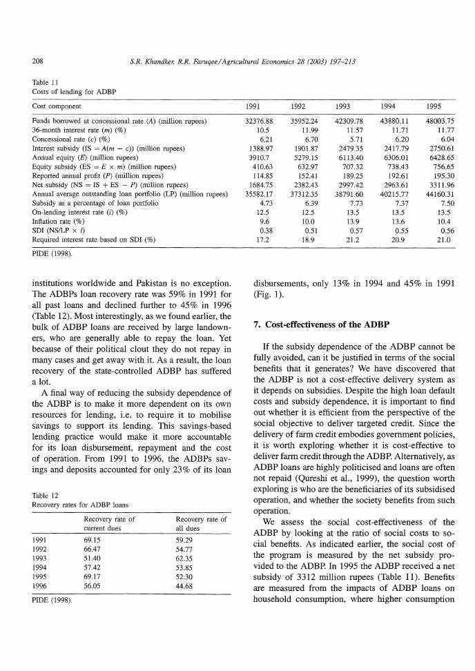
two subsidies plus equity subsidy calculated from an­nual equity. The net subsidy is the subsidy after the profit is netted out. As Table ll shows, the net sub­sidy of ADBP increased from 1685 million rupees in 1991 to 3312 million rupees in 1995 (Qureshi et al., 1999). This increase was due to the increase in bor­rowing funds and equity that occurred while interest rates remained largely constant. The average subsidy was 4.7% of the loans outstanding in 1991 and 7.5% in 1995. 15

The nominal interest rate of ADBP loans increased slightly from 1991 to 1995 and from 12.5 to 13.5%. The rate of inflation during this period increased from 9.6% in 1991 to 13.9% in 1993, and then decreased to 10.4% in 1995. The data clearly show that the real rate of interest on an ADBP loan was negative for most of the time during the study period. So one way of reduc­ing the subsidy dependence of the ADBP would be to increase the nominal interest rate it changes. To de­termine how much the nominal rate of interest would have to be increased to eliminate the subsidy, we use the subsidy dependence index (SDI) measure (Yaron, 1992). The SDI is expressed as the net subsidy (total subsidy less accounting profit) as a percentage of inter­est income received from on-lending (which is in tum defined as the average loan outstanding times the nom­inal interest rate). The SDI measures the percentage in­crease in the average on-lending interest rate required to eliminate all subsidies in a given year while keep­ing the return on equity equal to the non-concession borrowing cost. Between 1991 and 1995, the SDI in­creased from 0.38 to 0.56. Thus, in order to eliminate subsidy it receives, the ADBP would have had to in­crease the on-lending interest rate by 38% in 1991 and by 56% in 1995. Using the nominal rate for those years, this means that the nominal rate should have increased from 12.5 to 17.2% in 1991 and from 13.5 to 21% in 1995.

Another way of reducing subsidy dependence is to improve the loan recovery rate. Loan recovery has been a major concern for all government-run credit

15 The subsidy provided to the ADBP is comparable with that of other successful financial institutions around the world. For example, the Grameen Bank of Bangladesh, which is a role model for micro-credit programs worldwide, enjoyed a subsidy rate of 5.6% in 1994 (Khandker, 1988). But unlike the Grameen Bank, ADBP loans are received mostly by large landholders.

208 S.R. Khandker, R.R. Faruqee/Agricultural Economics 28 (2003) 197-213

Table 11 Costs of lending for ADBP

Cost component

Funds borrowed at concessional rate (A) (million rupees) 36-month interest rate (m) (%) Concessional rate (c) (%) Interest subsidy (IS = A(m - c)) (million rupees) Annual equity (E) (million rupees) Equity subsidy (ES = E x m) (million rupees) Reported annual profit (P) (million rupees) Net subsidy (NS = IS + ES - P) (million rupees) Annual average outstanding loan portfolio (LP) (million rupees) Subsidy as a percentage of loan portfolio On-lending interest rate (i) (%) Inflation rate (%) SDI (NS/LP X i) Required interest rate based on SDI (%)

PIDE (1998).

institutions worldwide and Pakistan is no exception. The ADBPs loan recovery rate was 59% in 1991 for all past loans and declined further to 45% in 1996 (Table 12). Most interestingly, as we found earlier, the bulk of ADBP loans are received by large landown­ers, who are generally able to repay the loan. Yet because of their political clout they do not repay in many cases and get away with it. As a result, the loan recovery of the state-controlled ADBP has suffered a lot.

A final way of reducing the subsidy dependence of the ADBP is to make it more dependent on its own resources for lending, i.e. to require it to mobilise savings to support its lending. This savings-based lending practice would make it more accountable for its loan disbursement, repayment and the cost of operation. From 1991 to 1996, the ADBPs sav­ings and deposits accounted for only 23% of its loan

Table 12 Recovery rates for ADBP loans

1991 1992 1993 1994 1995 1996

PIDE (1998).

Recovery rate of current dues

69.15 66.47 51.40 57.42 69.17 56.05

Recovery rate of all dues

59.29 54.77 62.35 53.85 52.30 44.68

1991 1992 1993 1994 1995

32376.88 35952.24 42309.78 43880.11 48003.75 10.5 11.99 11.57 11.71 11.77 6.21 6.70 5.71 6.20 6.04

1388.97 1901.87 2479.35 2417.79 2750.61 3910.7 5279.15 6113.40 6306.01 6428.65

410.63 632.97 707.32 738.43 756.65 114.85 152.41 189.25 192.61 195.30

1684.75 2382.43 2997.42 2963.61 3311.96 35582.17 37312.35 38791.60 40215.77 44160.31

4.73 6.39 7.73 7.37 7.50 12.5 12.5 13.5 13.5 13.5 9.6 10.0 13.9 13.6 10.4 0.38 0.51 0.57 0.55 0.56

17.2 18.9 21.2 20.9 21.0

disbursements, only 13% in 1994 and 45% in 1991 (Fig. 1).

7. Cost-effectiveness of the ADBP

If the subsidy dependence of the ADBP cannot be fully avoided, can it be justified in terms of the social benefits that it generates? We have discovered that the ADBP is not a cost-effective delivery system as it depends on subsidies. Despite the high loan default costs and subsidy dependence, it is important to find out whether it is efficient from the perspective of the social objective to deliver targeted credit. Since the delivery of farm credit embodies government policies, it is worth exploring whether it is cost-effective to deliver farm credit through the ADBP. Alternatively, as ADBP loans are highly politicised and loans are often not repaid (Qureshi et al., 1999), the question worth exploring is who are the beneficiaries of its subsidised operation, and whether the society benefits from such operation.

We assess the social cost-effectiveness of the ADBP by looking at the ratio of social costs to so­cial benefits. As indicated earlier, the social cost of the program is measured by the net subsidy pro­vided to the ADBP. In 1995 the ADBP received a net subsidy of 3312 million rupees (Table 11). Benefits are measured from the impacts of ADBP loans on household consumption, where higher consumption

S.R. Khandker, R.R. Faruqee/Agricultural Economics 28 (2003) 197-213 209

16000

14000 .. .. .. 12000 D.

::> a: 0

i[ 10000

= Ill 0 D. 8000 .. "0 "0 c .. c 6000 .. E .. 2! ::> 4000 .1:1 .!!! Q

2000

0 1990

.........._Disbursement

-Deposit

1991 1992 1993

Years

1994 1995 1996 1997

Fig. 1. Disbursement and deposit trends for ADBP loans.

means a reduction of poverty. 16 Social benefits can be calculated in two ways: one based on average benefits accruing to all borrower households, and the other based on the sum of benefits accruing to differ­ent groups of households based on their operational holdings. Based on operational holdings, households are categorised into three groups: smallholders (op­erational holding up to 12.5 acres), medium holders (operational holding between 12.5 and 25 acres) and large holders (operational holding over 25 acres). Like the impact estimates based on the entire sample of households, two-stage regressions were carried out for the three groups of households separately to esti­mate the marginal returns to consumptions for these households.

The ADBP had a total loan portfolio of 44,160.31 million rupees in 1995 and we assume that the dis-

16 The impact of credit on consumption is taken as a measure of social benefit for calculating cost-benefit ratios. Credit is used for production and consumption. The loan used for consumption increases consumption directly by helping consume more and indirectly by increasing labour productivity through sustaining the consumption required for maintaining physical strength of a person. Credit used for production increases income and net worth which in turn help increase the consumption. Hence, the consumption impacts measure the appropriate social benefits of credit.

tribution of this portfolio among different operational holding was the same as observed in our sample. Us­ing sample weights we determine the amount of credit that each group received from the ADBP. This amount, when multiplied by the marginal return to consump­tion, provides an average amount of benefit for different categories of ADBP borrowers. Aggregating benefits across groups results in a program-level ben­efit of 2485 million rupees, leading to a society-level cost-benefit ratio of 1.347 (3312/2458) (Table 13). Hence, the social cost of ADBP lending exceeded the social benefit by as much as 35% in 1995. This is very similar to the estimated cost-benefit ratio (1.331) of ADBP lending based on the single equation run for the entire sample. We conclude that ADBP lending is not socially profitableP

Since the social benefit of ADBP lending is posi­tive only for small producers, the question is whether

17 Note that this is calculated using the estimates of marginal returns. Ideally one should use the average returns, which, under the assumption of diminishing returns, are higher than marginal returns. If average returns are higher than marginal returns, it is possible that the ADBP may be cost-effective. Nonetheless, based on the same type of analysis, the ADBP seems less cost-effective than the Grameen Bank of Bangladesh, which is highly successful in reaching the poor households, especially women.

Table 13 Cost-effectiveness of ADBP lending based on actual distribution of loans

ADBP annual Borrower Share of Amount received Marginal Gains accrued Benefit Cost Cost-benefit ratio loan out-standing type loans (million rupees) return (million rupees) (total of gains accrued) (annual subsidy) (million rupees) (million rupees) (million rupees)

44160.3 Small 0.420 (1.00) 18547.2 (44160.3) 0.130. 2411.1 (5740.8) Medium 0.412 (0) 18194.0 (0) 0.001 18.2 (0) 2457.7 (5740.8) 3311.7 1.347 (0.577) Large 0.168 (0) 14189.3 (0) 0.002 28.4 (0) Aggregate 1.00 44160.3 o.o55• 2488.8 2488.8 3311.7 1.331

Figures in parentheses are based on the assumption that total lending is disbursed only to borrowers with positive and significant returns (in this case smallholders). • Estimates are significant at 5% level.

N

0

!"-'> ?ll

~ ~ "' "' ?ll ?ll ~

~ ~

i ~ ?;1

~ ~-

N Oo

~ ...... 10

l'l N ......

'""

S.R. Khandker, R.R. Faruqee/Agricultural Economics 28 (2003) 197-213 211

it would be socially profitable if it were disbursed ex­clusively to smallholders. The re-calculation of the social benefits and the cost-benefit ratio for ADBP lending shows that benefits exceed costs by 73% (the cost-benefit ratio is 0.58) in the case (Table 13). There­fore, even if the ADBP is subsidised, a better targeting of its operations could make it worth supporting by society. Of course, this does not mean that the ADBP must receive subsidies. It means that if a subsidy is a necessary condition for running a highly targeted scheme in rural areas, the generated benefits should be large enough so that society would find it worth sup­porting. It follows that the ADBP must be redesigned to reach the poor households and small producers. If it cannot improve outreach, then its current subsidy de­pendence cannot be justified, as its loans are largely benefiting medium and large landlords, who should not qualify for receiving subsidised credit.

8. Conclusions and policy implications

The purpose of this study was to provide economet­ric evidence on the impact of farm credit on house­hold welfare and the role of the state-owned ADBP. Like past studies, we find statistically significant ef­fects of institutional credit not only on the determi­nants of agricultural output, but also on household consumption and other household welfare indicators. Like earlier studies, we also find evidence of poor access of small landowners to formal credit. Clearly, formal lenders are biased towards larger farmers who can provide collateral, and as a result smaller and ten­ant farmers are left out. In Pakistan, large landowners, who constitute only 4% of rural households, account for 42% of formal finance, while subsistence house­holds, who constitute more than 69% of rural house­holds, receive only 23% of formal loans.

Formal loans are taken mostly for production pur­poses. Data shows that only 5% offormalloans finance consumption, and an overwhelming 95% support pro­duction (88% to farm and 7% to non-farm produc­tion). In contrast, 56% of informal loans were used for consumption, while 44% were used to support produc­tion. These production loans are used for income gen­eration, which can then support higher consumption. Thus, the effect of such loans on consumption is indi­rect. If household consumption is taken as a measure

of household welfare, the estimated marginal impact of formal loans on consumption is substantial. An ad­ditional 100 rupees of loan from a formal source such as the ADBP can increase per capita consumption by as much as 5 rupee. When the impacts of credit are estimated by operational landholding, the distribution of benefits is found to vary by the size of operational holding. In particular, the returns to consumption of borrowing from the ADBP are as much as 13% for smallholders (who own up to 2.5 acres of land) com­pared with 0% for medium and large farmers.

Is ADBP lending cost-effective? Using some esti­mates of the net cost that is not recovered from its in­come, we find that the ADBP is subsidised, even more subsidised than the Grameen Bank of Bangladesh, a highly donor dependent and poor-focused micro-credit program. 18 Using the subsidy provided to the ADBP as the cost of delivering formal credit to rural house­holds, estimates show that the government of Pakistan has to provide a subsidy of 7.5% of its loans outstand­ing (as of 1995) to support ADBP operations; oth­erwise the ADBP cannot run its business. Reduction of subsidies could be accomplished through cost sav­ings such as reducing loan default costs and by raising nominal interest rates to a level that at least reflects a positive real on-lending rate. The ADBP could also practice self-reliance by relying more on mobilised de­posits and savings, and less on government and donor resources for on-lending.

More importantly, the ADBP may find it necessary to extend its outreach so as to reach out the poor and the asset-less, whose repayment record is better than that of large holders. Results suggest that institutional credit is productive, but that its outreach is limited to a small proportion of the population that perhaps does not need subsidised credit. There is little doubt that credit channelled in the right direction has significant anti-poverty effects, and that broadening the outreach of formal lending institutions would represent a step in the right direction.

Acknowledgements

The authors would like to thank Robert Moffit, Mark Pitt, participants of a seminar in Islamabad, and two

18 For a case study on Bangladesh's Grameen Bank see Khandker (1988).

N ;::;

Table A.l Second stage results: impacts of ADBP borrowing on household outcomes

Explanatory variables Annual Annual crop Annual net Non-land asset Male labour Female labour consumption production cost production (rupees) supply supply

,.., ~

(rupees) (rupees) output (rupees) (h/month) (h/month) ~

Total ADBP borrowing (rupees) 0.004 (2.378) O.IIO (6.855) 0.088 (2.480) 0.005 (0.667) 0.004 (0.593) 0.098 (6.I58) "" ;:,

Maximum male education 0.020 (7.52I) -O.I03 (-4.077) -O.lll (-1.994) 0.062 (5.602) O.OI8 (1.5I2) -O.I48 (-5.896) ~ in household (years) ""

~ Maximum female education 0.030 (11. 728) -0.048 ( -1.930) -0.09I ( -1.649) 0.070 (6.27I) -0.048 ( -4.053) -O.I23 (-4.934) ~ in household (years)

~ Age of head (years) O.OOI (1.310) O.OOI (0.305) -0.011 ( -1.129) 0.003 (1.383) -O.OOI (-0.334) O.OOI (0.182) i:! Land owned by household (acre) O.OOI (7.426) 0.02I (11.850) O.OI5 (3.889) 0.005 (6.250) 0.00 I ( 1.652) -0.007 (-3.908) "" "' "' Price of rice (rupees/kg) 0.003 (1.748) 0.059 (3.349) 0.042 (1.076) 0.005 (0.685) 0.029 (3.460) 0.111 (6.3I2) :;;: Price of wheat (rupees/kg) -0.005 ( -1.469) -0.092 (-2.784) -0.033 ( -0.448) -0.033 (-2.282) -0.037 (-2.382) -0.060 ( -1.834) "" ;:;, Price of gram/pulses (rupees/kg) 0.005 (4.032) -0.053 ( -4.265) -0.022 ( -0.808) O.OOI (O.I93) 0.006 (0.990) -0.027 (-2.223) " ;::

Price of milk and milk products -0.002 (-0.6I2) -0.026 ( -0.929) -0.040 ( -0.637) 0.02I (1.653) -0.028 (-2.I05) 0.022 (0.803) i! (rupees/kg) ~

Price of vegetable oil (rupees/kg) O.OOI (1.4I6) 0.04I (5.803) O.OI9 (1.226) O.OOI (0.174) 0.005 ( 1.499) 0.006 (0.838) ~ c Price of beef (rupees/kg) -0.002 (-2.613) 0.007 (0.884) O.OII (0.608) O.OOI (0.3I5) O.OIO (2.63I) 0.008 (1.025) ;:,

c Price of fish (rupees/kg) 0.003 (5.336) -0.006 (-1.210) O.OI2 (1.033) -0.002 ( -0.858) -0.0005 (-0.192) -0.003 ( -0.540) ~

~-Price of vegetables (rupees/kg) 0.007 (3.869) -0.073 (-3.938) -0.002 ( -0.046) 0.013 (1.638) -0.027 (-3.I53) -0.086 ( -4.675)

"' Price of brown sugar (rupees/kg) -0.0001 (-0.047) -O.I44 (-9.013) -O.I89 (-5.366) 0.030 (4.179) -0.049 ( -6.505) -O.I74 (-I0.930) Oo

'N Price of fruits (rupees/kg) O.OOI (0.967) 0.066 (6.108) 0.066 (2.764) 0.004 (0.854) 0.010 (1.938) O.D38 (3.534) 0

Price of maize (rupees/kg) 0.0003 (0.596) -O.OOI (-0.199) -0.004 (-0.371) -0.006 (-2.884) 0.002 (0.888) -0.009 (-1.889) _§ Price of other grains and cereals -O.OOOI (-0.509) -0.008 (-3.I85) 0.00 I (0.098) O.OOI (0.870) -O.OOI (-0.776) O.OIO (3.848) ._

'0

(rupees/kg) ['1 "' ._

Constant 9.293 (132.400) 9.358 (I3.787) 6.136 (4.075) 8.674 (28.869) 8.529 (26.678) Il.300 (I6.728) v,

Adjusted R2 0.418 0.152 0.376 0.13I O.I05 0.084 Observations 4380 4380 4380 4380 4380 4380

PIDE (1998).

S.R. Khandker; R.R. Faruqee/ Agricultural Economics 28 (2003) 197-213 213

anonymous reviewers of this journal for helpful com­ments and suggestions. They also would like to thank Ananya Basu, Tulika Narayan, and Hussain Samad for excellent computer and research assistance. Views ex­pressed in the paper are entirely the authors' and do not reflect in any way views of the World Bank.

Appendix A

Second stage results: impacts of ADBP borrowing on household outcomes are shown in Table A.l.

References

Adams, D.W., Fitchett, D.A. (Eds.), 1992. Informal Finance in Low-Income Countries. Westview Press, Boulder, CO.

AERC (Applied Economics Research Centre), 1998. Borrowers' Transaction Cost Study. Final Report: Rural Financial Market Study (Phase II), University of Karachi, Karachi, Pakistan.

Aleem, 1., 1990. Imperfect information, screening, and the costs of informal lending: a study of a rural credit market in Pakistan. World Bank Econ. Rev. 4 (3), 329-349.

Binswanger, H.P., Rosenzweig, M.R., 1986. The behavioural and material determinants of production relations in agriculture. J. Dev. Stud. 32 (October), 503-539.

Binswanger, H.P., Khandker, S.R., 1995. The impact of formal finance on the rural economy of India. J. Dev. Stud. 32 (2), 234-262.

Braverman, A., Guasch, J.L., 1989. Rural credit in LDCs: issues and evidences. J. Econ. Dev. (Korea) 14 (June), 7-34.

Brugger, E., Rajpatirana, S. (Eds.), 1995. New Perspectives on Financing Small Business in Developing Countries. ICS Press, San Francisco.

Carter, M.R., 1988. Equilibrium credit rationing of small farm agriculture. J. Dev. Econ. 28, 83-103.

Carter, M.R., Weihe, K.D., 1990. Access to capital and its impact on agrarian structure and productivity in Kenya. Am. J. Agric. Econ. 72, 1146-1150.

Christen, R.P., Rhyne, E., Vogel, R., 1994. Maximising the outreach of microenterprise finance: the emerging lessons of successful programs. IMCC Paper, Washington, DC.

Feder, G., Lau, L.J., Lin, J.Y., Luo, X., 1990. The relationship between credit and productivity in Chinese agriculture: a microeconomic model of disequilibrium. Am. J. Agric. Econ. 72, 1153-1157.

Ghate, P., 1992. Informal Finance: Some Findings from Asia. Oxford University Press, Oxford.

Hoff, K., Stiglitz, J.E., 1990. Introduction: imperfect information and rural credit markets: puzzles and policy perspectives. World Bank Econ. Rev. 4 (3), 235-251.

Hulme, D., Mosley, P. (Eds.), 1996. Finance Against Poverty. Routledge, London.

Hussain, 1., Demaine, H., 1992. How informal credit offers greater benefits to farmers: an inquiry into rural credit markets in Pakistan. Asian Institute of Technology, Division of Human Settlements Development, Bangkok, Thailand.

Khandker, S.R., 1988. Fighting Poverty with Microcredit: Experience in Bangladesh. Oxford University Press, New York.

Malik, S.J., Mushtaq, M., Gill, M.A., 1991. The role of institutional credit in the agricultural development of Pakistan. Pakistan Dev. Rev. 30, 1039-1048.

McKernan, S.-M., 1996. The impact of micro-credit programs on self-employment profits: do non-credit program aspects matter? Draft, Brown University.

Otero, M., Rhyne, E., 1994. The New World of Microenterprise Finance. Kumarian Press, West Hartford, CT.

PACC (Pakistan Agricultural Census Commission), 1973. Rural credit Survey. Government of Pakistan, Lahore.

PACC (Pakistan Agricultural Census Commission), 1985. Rural credit Survey. Government of Pakistan, Lahore.

PACC (Pakistan Agricultural Census Commission), 1995. Rural Credit Survey. Government of Pakistan, Lahore.

PIDE (Pakistan Institute of Development Economics), 1998. Study on Economic Performance, Cost Structure, and Programme Placement of Bank Branches in Pakistan. Draft Final Report prepared for State Bank of Pakistan, Islamabad, Pakistan.

Pitt, M.M., Khandker, S.R., 1996. Household and intrahousehold impact of the Grameen Bank and similar targeted credit programs in Bangladesh. World Bank Discussion Paper No. 320, Washington, DC.

Pitt, M.M., Khandker, S.R., 1998. The impact of group-based credit programs on poor households in Bangladesh: does the gender of participants matter? J. Political Econ. 106 (5), 958-996.

Qureshi, S., Nabi, 1., Faruqee, R., 1999. Improving rural finance. In: Faruqee, R. (Ed.), Strategic Reforms for Agricultural Growth in Pakistan. The World Bank, Washington, DC.

Udry, C., 1990. Credit markets in northern Nigeria: credit as insurance in a rural economy. World Bank Econ. Rev. 4 (3), 251-269.

von Braun, J., Malik, S., Zeller, M., 1993. Credit markets, input support policies and the poor; insight from Africa and Asia. International Food Policy Research Institute, Washington, DC.

Yaron, J ., 1992. Successful rural financial institutions. World Bank Discussion Paper. No. 150, Washington, DC.

Zuberi, H., 1989. Production function, institutional credit and agricultural development in Pakistan. Pakistan Dev. Rev. 28, 43-56.