NBER WO~G PAPER SERIES

THE DETERMINANTS OF THE CHOICEBETWEEN FIXED AND FLEXIBLE

EXCHANGE-RATE REGIMES

Sebastian Edwards

Working Paper 5756

NATIONAL BUREAU OF ECONOMIC RESEARCH1050 Massachusetts Avenue

Cambridge, MA 02138September 1996

This is a revised version of a paper presented at the NBER East Asian Seminar on Economics. Thiswork is part of the NBER’s Project on International Capital Flows, which receives support from theCenter for International Political Economy. I am gratefil to Anne Krueger and Andrew Rose forcomments. I am also th~ful to seminm participants at Duke and Johns Hopkins for helpfulcomments. I am grateful to Fernando Losada and Daniel Lederman for their invaluable researchassistance. I also benefited from discussions with Miguel Savastano. This paper is part of NBER’sresearch program in International Finance and Macroeconomics. Any opinions expressed are thoseof the author and not those of the National Bureau of Economic Research.

O 1996 by Sebastian Edwards. All rights reserved. Short sections of text, not to exceed twoparagraphs, may be quoted without explicit permission provided that fill credit, including 0 notice,is given to the source.

NBER Working Paper 5756September 1996

THE DETERMINANTS OF THE CHOICEBETWEEN FIXED AND FLEXIBLE

EXCHANGE-RATE REGIMES

ABSTRACT

In recent years, analysts and policy makers alike have been evaluating the nexus between

exchange rates and macroeconomic stability. Among the most important questions asked is why

have some countries adopted rigid, including fixed, exchange-rate regimes, while others have opted

for more flexible systems? This paper addresses this question from a political economy perspective,

both theoretically and empirically.

The model assumes that the monetary authority minimizes a quadratic loss function that

captures the trade-off between inflation and unemployment. This framework is initially applied to

the case where monetary authorities must choose between a (permanently) fixed and a flexible

exchange-rate regime. In selecting the regime, the authorities are assumed to compare the expected

losses under each scenario. The model is subsequently extended to cover the somewhat more

complicated case where the authorities must choose between fixed-but-adjustable and flexible

exchange-rate regimes. In this latter case, potential political costs of abandoning the pegged rate

are taken into account. In the empirical section, an unbalanced panel data set of 63 countries from

1980-1992 is used to estimate a series of probit models, with a binary exchange-rate regime index

as the dependent variable, Among the most important explanatory variables were measures of

countries’ historical degree of political instability, various measures of the probability of abandoning

pegged rates, and variables related to the relative importance of real (unemployment) targets in the

preferences of monetary authorities. The regression results support the political economy approach

developed in the theoretical discussion.

Sebastian EdwardsAnderson Graduate School of ManagementUniversity of California, Los AngelesLos Angeles, CA 90095and NBERsedwards@agsm.ucla. edu

I. Introduction

In most developing and transitional economies, exchange rate issues have tended to

dominate macroeconomic policy discussions during the last few years. In particular, attention

has focused on two broad problems: first, how to define, measure, detect and correct situations of

real exchange i-ate misalignment and overvaluation; and second, on understanding the

relationship between nominal exchange rates and macroeconomic stability. Issues related to rea/

exchange rate misalignment have been central, for example, in debates that preceded the

devaluation of African currencies participating in the CFA franc zone in the early 1990s, in post

mortems of the Mexican crisis of December 1994, and in recent analyses of the Argentine

stabilization program of 1991.

Regarding the relationship between exchange rates and macroeconomic stability, four

specific questions have attracted the attention of analysts and policy makers:

(a) Why have some countries adopted rigid, including fixed, exchange-rate

regimes, while others have opted for more flexible systems?;

(b) Do fixed exchange-rate regimes impose an effective constraint on monetary

behavior and, thus, result in lower inflation rates over the long run?;

(c) Are exchange-rate-based stabilization programs superior to money-based

stabilization programs?; and,

(d) How should exchange-rate-based stabilization programs actually be designed’?

The first two issues deal with the long run, while the third one is related to the short run,

transitional consequences of stabilization programs. 1 All four issues, however, have important

implications for a country’s macroeconomic performance and growth. Moreover, most of these

questions are intimately related to political economy and institutional considerations.

This paper deals with the first question from a political economy perspective. I ask. for

example, why does Austria have a fixed exchange rate, while the U.K. has a flexible one’? And.

why has Argentina chosen a fixed exchange rate, while her neighbor Chile has a flexible-cum-

bands system? More generally, in December 1992, why did eighty-four countries (out of 167

reported in the IMF’s International Financial Statistics) peg their currencies to a major currency

‘ Bruno ( 1991) covers analytical issues related to questions b-c. See also Sachs (1996). On the selection

of exchange rate regimes see Corden (1994), Edison and Melvin (1990), and Isard (1995),

or a currency composite? The theoretical discussion, presented in section II, emphasizes the role

of credibility, politics and institutions. In the empirical analysis (section III) I use a large cross-

country, panel data set to analyze empirically the determinants of the choice of regime.

II. The Political Economy of Exchange-rate regimes

In this section I develop a simple theoretical framework for analyzing the selection of

an exchange-rate regime. The analysis relies on the existence of a trade-off between

“credibility” and “flexibility”, and assumes that a pegged exchange-rate sys tern allows the

authorities to resolve, at least partially, the time inconsistency problem. I assume that policy

makers minimize a loss function defined over a monetary variable -- inflation -- and a real

variable -- say, unemployment. In order to simplify the discussion I initially assume that the

two alternative regimes are a flexible or a permanently fixed exchange-rate system. I then

extend the analysis to the case where the two options are a flexible regime or a pegged-but-

adjustable regime. In this case I assume that the abandonment of the pegged exchange rate

entails important political costs.

II. 1 Fixed or Flexible ? A Simple Framework

Assume, for simplicity, that the monetary authority must choose between two nominal

exchange-rate regimes: (permanently) fixed or flexible. Assume that the authorities take into

account the expected value of a loss function under the two alternative systems, Consider the

case where the loss function is quadratic and depends on inflation (n) squared and on squared

deviations of unemployment (u) from a target value (u*).* The model is given by equations (1)

through (5):

L= E(n2+p(u-u*)2); p>O.

u=u’-e( n-m) +~(x -x’); E(x) = X’,v(x) = 02.

2 This type of approach has been adopted, with some variants, by a number of authors

example, Persson and Tabel lini (1990), Devarajan and Rodrik (1992) and Frankel (1995).

(1)

(2)

See, for

u* < u’ (3)

u = E(n) + aE(x - X’) (4)

(5)n=~d+(l-~)m.

Equation (1) is the loss function. Equation (2) states that the observed rate of unemployment

(u) will be below the natural rate (u’) if inflation exceeds wage increases -- (n-m)> O -- and if

external shocks (x) are below their mean (x’). Variable x can be interpreted as a composite of

terms of trade and world interest rate shocks. It is assumed to have a variance equal to 02.

Equation (3) establishes that the target rate of unemployment u* is below the natural rate u‘,

Equation (4) implies that agents are rational in setting wage increases (a< O), and equation (5)

defines inflation as a weighted average of the rate of devaluation d and the rate of wage

increases u. Under fixed rates d is by definition equal to zero, while under flexible rates the

authorities set d according to an optimal devaluation rule. 3

The model’s solution depends on the sequence in which decisions are made. Assume

that workers determine @ before they observe x, d or n. The government, on the other hand,

sets its exchange rate policy after both u and x are observed. The government’s objective is

to set its exchange rate policy so as to minimize the value of the loss function (1). The

solution in the case of fixed exchange rates is:

~=() (6.1)

(6,2)u=u’+~ (x-x’).

These results assume that the fixed exchange-rate system allows the government to solve its

credibility problem, by providing a precommitment technology.

3 A limitation of this approach is that it assumes that fixed rates are unchangeable. The case of apegged but adjustable regime can be handled assuming that the fixed rule has escape clauses, See Floodand Isard (1989).

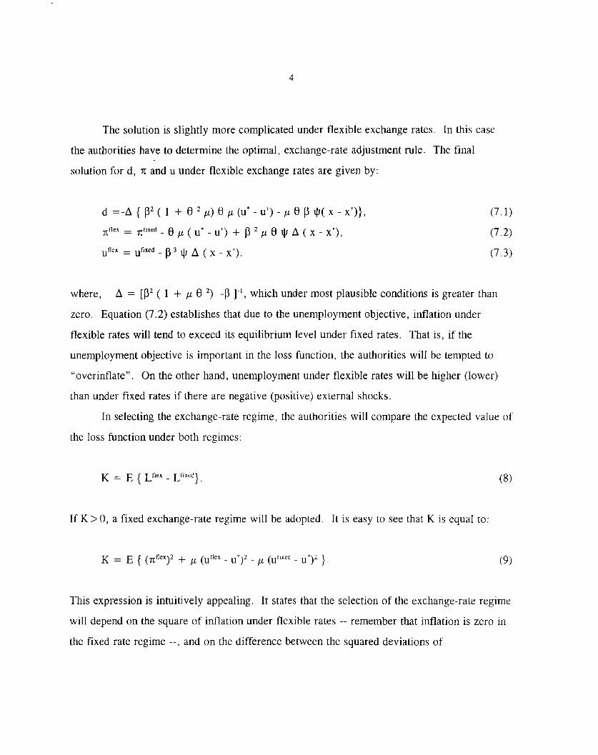
The solution is slightly more complicated under flexible exchange rates. In this case

the authorities have to determine the optimal, exchange-rate adjustment rule. The final

solution for d, n and u under flexible exchange rates are given by:

d=-A{~2( l+62p)6p (u*-u’)-p6~ $(X-X’)}, (7.1)

~flex = ~fixed -6p(u*- u’)+ p2pe~A (x-x’), (7.2)

Uflex = Ufixed -~3$A (x-x’). (7.3)

where, A = [~’ ( 1 + p (3 2, -~ ]-1, which under most plausible conditions is greater than

zero, Equation (7.2) establishes that due to the unemployment objective, inflation under

flexible rates will tend to exceed its equilibrium level under fixed rates. That is, if the

unemployment objective is important in the loss finction, the authorities will be tempted to

“overinflate”. On the other hand, unemployment under flexible rates will be higher (lower)

than under fixed rates if there are negative (positive) external shocks.

In selecting the exchange-rate regime, the authorities will compare the expected value of

the loss function under both regimes:

K = E { Lflex- Lfixed},

If K >0, a fixed exchange-rate

(8)

regime will be adopted. It is easy to see that K is equal to:

K = E { (n””)’ + p (uflex- u“)’ - p (ufix’d- u“)z } (9)

This expression is intuitively appealing. It states that the selection of the exchange-rate regime

will depend on the square of inflation under flexible rates -- remember that inflation is zero in

the fixed rate regime --, and on the difference between the squared deviations of

unemployment from their respective targets. After some manipulations equation (9) can be

rewritten as:

K = (6 p)z (U* -U’)2 - y 02, (lo)

where y is a positive function of A, ~, p, O and $. For K to be positive, and thus for fixed

rates to be preferred, the country’s “employment ambition” -- measured by (u* - u‘ ) -- has to

be “large enough”. More specifically, it has to exceed the variance of the external shocks.

On the other hand, if 02 is high enough, K can be negative indicating that flexible rates are

preferred. This would allow the authorities to reduce the deviation from its unemployment

target, An important question in the empirical evaluation of this (and related) models is how

to measure the degree of “ambition” of the authorities’ unemployment target -- (u* - u‘ ). I

take up this issue in section III.

II. 2 Flexible vs. Pegged-but-Adjustable Excltange-rate regimes

The preceding analysis assumed that under a fixed regime the nominal exchange rate

would never be altered. This is, of course, a major simplification. In reality, under fixed

exchange rates, governments always have the choice of abandoning the peg. This possibility can

be captured formally by assuming that the authorities follow a rule with some kind of escape

clause. In other words, the nominal exchange rate will be maintained at its original level under

certain circumstances. However, if these circumstances change markedly, the peg will be

abandoned. This means that at any moment in time there is a positive probability that the pegged

rate will be altered. This type of arrangement underlied the original Bretton Woods system that

ruled the international monetary system from 1948 to 1973. According to the original IMF

Articles of Agreement, a country could alter its peg if it was facing a “fundamental

disequilibrium”. In this section I sketch the analytics of this case.

Assume that ex ante a country can choose between two possible regimes: flexible nominal

rates (f) or pegged but adjustable rates (p). Also consider a two-period economy, where under a

pegged regime there is a positive probability that the peg will be abandoned at the end of the first

(or beginning of the second) period. The probability of abandoning the peg is denoted by q, and

the discount factor by ~. As in the preceding analysis, assume that the authorities have a distaste

for both inflation and for deviations of unemployment from a target level.

Assume further that the authorities will incur a political cost equal to C if the peg is

indeed abandoned. This assumption captures the stylized fact, first noted by Cooper (1971), that

stepwise devaluations have usually resulted in serious political upheaval and, in many cases, in

the fall of the government.4 The magnitude of this cost will, in turn, depend on the political and

institutional characteristics of the country, including the degree of political instability. In

politically unstable countries a major economic disturbance, such as the abandonment of a parity

that the authorities have promised to defend, will tend to have major political consequences. For

example, this can explain why the vast majority of stepwise devaluations take place during the

early years of an administration, when its degree of political popularity is higher.~ The degree of

political instability will also affect the government’s discount factor. In more unstable countries

the authorities will tend to be more impatient, discounting the future more heavily. This means

that denoting the degree of political instability

c = c(p);

P = P(P);

by p, we can write:

with C’ > 0, (11)

with ~’ < 0. (12)

In this two period economy, the loss function under flexible rates is (where the notation is

consistent with that used in the

4 Cooper reports that more

previous section):

than two thirds of the finance ministers that engineered the devaluations lost

their jobs within two months of the devaluation. See also Edwards (1994),

5 Using a broad sample of stepwise devaluations, Edwards (1994) found that in presidential democracies

77% of the devaluations took place within the first 18 months of new governments; this figure is 70% forparliamentary democracies, and only 43% for undemocratic regimes.

Lfl’x = y(n’)z + ~(UF-U*)2 + ~ (y (nF) (+12+ p [(UF),+L-U*]2), (13)

where y is a parameter that captures the degree of distaste for inflation.

The loss function under a pegged rate regime is:

Lpegged= y (np )2 + p (Up- U*)2+ ~ {(1-q)(y(np)L+12+ jA[(UP)L+l- U*]2) +

+ q (y (nD),+12+ p [(uD),+l - U*]2) + qc}, (14)

where the superscript D refers to the value of a specific variable in the second period, under

the devaluation scenario. If the escape clause is exercised and the peg abandoned, we assume

that the country moves into a flexible regime. That is, once the peg is abandoned, inflation

and unemployment in the second period will be determined as under a flexible system. b

In order to simplify the discussion and concentrate on the selection of the exchange-rate

regime, I do not specify explicitly the process governing the decision to use the escape clause.

As in equation (8) in the preceding section, the regime decision rule will be based on an ex

ante comparison between both loss functions:

K = E {LfleX- LPegged}, (15)

If K>O, then the pegged but adjustable regime is preferred. Some simple manipulation yields:

K = y(~F)2 + p [(KF)2-(KP)2]~ ~ (]-q) Y(7CF)L+I 2 +

+ ~ (1-q) P [(KF), +l 2- (Kp),+l 2]- q~c. (16)

b The rate of inflation will be higher under pegged-but-adjustable regime than under the (unrealistic)“forever” fixed system considered in section II. 1. This is because under pegged regimes the public’s expectedrate of inflation (in period 2) will explicitly take into account the probability that the peg will be abandoned:

E(i’cp),+l = q (nD),+, + (1 - q) (rip),+].

Where (K’)2= (UF- u*) 2 and (Kp) 2= (up - U*)2. From the analysis in the previous section it

follows that [(KF)2- (Kp)2 ]<0 and that [(K’),+, 2- (K’),+]2]< O. From equation(16) it is

possible to derive a number of hypotheses regarding the likelihood of a country choosing a

pegged-but-adjustable exchange-rate regime. A higher rate of inflation under flexible rates (in

either period) will increase the likelihood of a pegged regime being chosen. Moreover, with

other things given, a higher weight for inflation in the loss function -- that is a higher y -- will

also increme the probability of choosing a pegged exchange rate, On the other hand, an increase

in unemployment volatility under pegged rates, generated by a higher variance in the foreign

shock -- a higher u’, from the previous section -- will increase the likelihood that a flexible

system will be selected. A greater distaste for unemployment deviations -- that is a higher p --

will reduce the likelihood of selecting a pegged rate. Likewise, a higher cost of abandoning the

peg (C) will reduce the ex ante probability of selecting a pegged rate. Interestingly enough, a

higher probability of abandoning the peg -- a higher q -- will have an ambiguous effect on the ex

ante likelihood of choosing a pegged regime. This follows from the following expression:

K~= -~ y (nF)[+, 2- ~ p [(KF)t+l2- (Kp),+,2]- PC (17)

Notice that the presence of political costs of abandoning the peg (C) increases the likelihood

that this expression will be negative, making it more likely that a flexible regime will be

selected.

An important question relates to the relationship between political instability and the

selection of the exchange-rate regime. In principle there will be two offsetting forces. First, a

higher degree of political instability will increase the cost of abandoning the peg -- recall

equation (11 ) -- and thus will reduce the ex ante probability that a pegged regime will be

chosen. Second, a higher degree of instability will increase the authorities discount rate

(equation 12), reducing the importance of “the fiture” in their decision making process.

Formally:

K, = - ~qC’ + KO~’. (18)

While the first term is negative; the second can be either positive or negative, because the sign of

KP is indeterminate. This means that the way in which instability will affect the selection of an

exchange-rate system is an empirical question. I tackle this issue in the following section, where

I present the results of a number of probit regressions on panel data for 63 countries during 1980-

1992.

111. Empirical Results

In this section I use a cross-country, unbalanced panel data set from 1980-1992 to

analyze why some countries have adopted pegged exchange-rate regimes while others have

opted for more flexible systems. I estimate a number of probit equations to investigate

whether, among other factors, a country’s political and economic structure, including its

degree of political instability, its degree of openness, and the variability of export earnings,

help explain the selection of an exchange-rate regime. Two classes of independent variables

were used in the analysis: the first attempts to capture long term structural characteristics --

both political and economic --of these countries, and are assumed to change very slowly over

time. In the empirical analysis they are defined as an average for the decade prior to the one

included in the analysis. The second class of independent variables tries to capture, for each

country, the evolution of some key time series (see below for a discussion on how each

variable is actually defined).

Probit equations of the following type were estimated using an unbalanced panel data

set for 63 advanced and developing countries (see the appendix for the list of countries):

pegi, = ~7Pi + k’ QiL+ ~’ Ri[.l + Ei~, (19)

where subindexes i and t refer to country i in year t. Peg is an exchange-rate regime index

defined below. p, 1 and $ are parameter vectors; P are variables specifying national political

10

and economic characteristics. In order to avoid simultaneity problems these variables were

defined, in most cases, as averages for the previous decade (1970-1980). See the discussion

below for details. Q and R are variables (economic and structural) for which panel data are

available; while the Qs are timed at period t, the Rs are lagged one (or more) periods. This is,

mostly to reduce the pitfalls of simultaneity problems.

III. 1 Data

The empirical analysis poses some difficult data challenges. Chief among them are: (a)

classifying the broad variety of exchange-rate systems observed in the real world into two

broad categories -- pegged and flexible--; (b) measuring political instability; and (c) defining

measures of the authority’s incentives for “tying its own hands. ”

Defining exchunge-rate regimes

The ~F’s International Financial Statistics classifies countries according to their

exchange-rate system in three broad groups: (a) Countries whose currency is pegged either to

a single currency or to a currency composite. (b) Countries whose exchange-rate system has

limited flexibility “in terms of a single currency or group of currencies”. This group includes

a rather small number of countries that have adopted a narrow band, including those in the

ERM. In June of 1991, for example, only eleven countries were listed in this group. And (c),

countries with “more flexible” exchange-rate systems. This group includes countries where

the exchange rate is adjusted frequently according to a set of indicators, countries that float

independently and countries with “other managed floating” regimes.

In the empirical analysis presented in this paper, countries are classified according to

their exchange-rate regime in a binary fashion as “pegged” or “flexible”. A difficulty with

this approach, however, is that it is not entirely clear how the middle group -- that is nations

which according to the IMF have “limited flexibility ”-- should be classified. In order to deal

with this issue I have used two altermtive classifications. The first one considers as having a

pegged exchange-rate system only those countries classified by the IFS as such. Thus, a

variable pegl that takes a value of one for those countries, and zero for countries with “limited

11

flexibility” and “more flexible” regimes was defined. The second classification considers as

having a pegged regime those countries classified as such by the IFS, plus those with

“flexibility limited in terms of a single currency or group of currencies”. Variable peg2, then,

takes a value of one for “pegged” and “limited flexibility countries” and zero for those nations

with a “more flexible” regime.

Measuring Political InstabiliQ

Most empirically-based political economy studies have used rather crude measures of

political instability, including the number of politically motivated assassinations and attacks

(Barro 1991). Other studies have used the frequency -- either actual or estimated --of

government change as a measure of political turnover and instability (Cukierman et al. 1992). A

limitation of this type of measure, however, is that it treats every change in the head of state as an

indication of political instability, without inquiring whether the new leadership belongs to the

same, or opposing, party than the departing leader. In that sense, for example, the replacement of

a prime minister by another from the same party is considered to have the same meaning as a

change in the ruling p~y (Cukierman 1992).

In this paper I use two alternative measures of political instability. The first, POLINST,

corresponds to the most traditional approach, and is defined as the estimated frequency of

government change for 1971-1980. This variable has been used by Cukierman et al (1992). This

variable is measured for 1971-1982, and is assumed to capture the inherent degree of political

instability of each country. The second measure, POLTRAN, is a new index of political

instability that focuses on instances where there has been a transfer ofpower from a party or

group in office, to a party or group formerly in the opposition, also between 1972 and 1980.7

This index measures the instability of the political system by capturing changes in the political

leadership from the governing party (or group, in the case of non-democratic regimes) to an

opposition party. In constructing this index, a transfer of power is defined as a situation

where there is a break in the governing political party’s (or dictator’s) control of executive

7 The merits of this typeof indexwere first discussedin Edwardsand Tabellini(1994).

12

power. More specifically, under a presidential system a transfer of power would occur if a

new government headed by a party previously in the opposition takes over the executive.

Under a parliamentarian regime, a transfer of power is recorded when a new government

headed by a party previously in the opposition takes over, or when there are major changes in

the coalition so as to force the leading party into the opposition. However, when the

goverting coalition remains basically unaltered, even if the new prime minister belongs to a

party different from that of the outgoing prime minister, a transfer of power is not recorded.

Finally, in the case of single-party systems, dictatorships or monarchies, a transfer of power

only takes place if there are forced changes of the head of state. Appointments of a successor

by an outgoing dictator (as in Brazil during the 1970s) are not recorded as transfers of power.

As in the case of POLINST, this variable has a single value for each country, corresponding to

the period 1971-1980. By concentrating in the period immediately preceding the one used in

the probit analysis, potential endogeneity problems are reduced.

In addition to the two indexes of political instability, three indicators were used as

proxies of the extent of weakness of the government in office. The first one refers to whether

the party or coalition of parties in office have the absolute majority of seats in the lower house

of parliament, In any given year this indicator, called MAJ, takes a value of zero if the party

(coalition) does not have majority; it takes a value of one if it has majority; and takes a value

of two if the system is a dictatorship. A higher value of MAJ, then, reflects a stronger

government. In the cross-country regression the average of MAJ over 1971-1980 was used.

The second indicator of political weakness that we used is the number of political

parties in the governing coalition (NPC). This index takes a value of zero for monarchical or

dictatorial systems, and the number of parties participating in ruling coalitions under

democratic regimes (that is, if there is a single-party government NPC will take the value of

one). It is expected that the higher the number of parties in that coalition, the higher the

probability of conflict of interest across ministries and, thus, the higher tie reliance on the

inflation tax. The third indicator of government weakness is whether the government is a

13

coalition government or a single-party government (COAL). This index takes a value of zero

for dictatorships, a value of one for single-party governments and a value of two for coalition

governments.

Other Data

According to the model presented in section II, in addition to the political factors

discussed above, other variables that capture structural characteristics of an economy are

important in the process of selecting an exchange-rate system.

External shocks. Two alternative indices were used to measure the extent of external

shock variability. (a) A coefficient of variation of real export growth for 1970-1982, denoted

as CVEX, was constructed with raw data obtained from the IMF’s International Financial

Statistics (IFS). (b) A coefficient of variation of real bilateral exchange rate changes for 1970-

1982, EXVAR, was constructed from data obtained from the IFS. The use of these variables

in the regression amlysis presents a potential endogeneity problem. In order to minimize this

danger in the probit reported below, lagged values (for 1970-82) of these indexes were used.

It is expected that the coefficient of these variables in the probit regressions will be negative,

indicating that, as reflected in equation (10), countries with a more volatile external sector will

tend to select a more flexible regime.

In principle, the actual importance of external shocks should also depend on the degree

of openness of the economy -- more open countries are more “vulnerable” to external

disturbances, In order to consider this effect I added an interactive term between external

variability and the degree of openness, denoted as VAR_OPEN. The latter was defined as the

ratio of imports plus exports to GNP, and was constructed from data obtained from the IFS.

Degree of “Ambition” of the unemployment target: A cornerstone of the model

developed above -- and of most Barre-Gordon types of model -- is the idea that countries with

a very “ambitious” real (that is, unemployment) objective will have an incentive to “tie their

own hands”, in order to solve their credibility problem. That is, with other things given, they

will have a greater incentive to select a pegged exchange-rate system. It is not easy, however,

. . .

14

to measure empirically this degree of” ambition”. In particular, only a handful of countries

have data on unemployment. For this reason I have used lagged, average real rates of growth

of GDP (for 1970-1980) as a proxy for the countries incentives to “tie their own hands”. I

assume that, with other things given, countries with a historically low rate of growth will be

more tempted to “overinflate” as a way to accelerate growth, even in the short run. If this is

the case, then low growth countries will have an incentive to “tie their own hands” as a way to

avoid falling into this temptation. It is expected that the coefficient of GROWTH will be

negative in the probit regressions. Naturally, the use of growth as a regressor raises the

possibility of endogeneity. It is indeed possible that the exchange-rate regime will, per se,

affect economic performance, including growth. In order to avoid this problem I use lagged

averages (by one decade) of growth rates in the estimation of the probit models (19). To the

extent that this variable tries to capture the historical and structural incentives faced by a

country to tie its authorities’ hands, the use of lagged averages is, indeed, appropriate.

Probability of abandoning rhepeg, (or abili~ of maintaining it): As discussed in the

preceding section a higher probability of abandoning the peg -- a higher q -- can, in principle,

affect the likelihood of selecting a pegged rate either positively or negatively. Since it is not

possible to observe q directly, four variables that capture the probability of having a

devaluation were considered in the empirical analysis: (a) the historical rate of inflation.

Countries with a history of rapid inflation will tend to have a greater propensity to devaluing.

This variable is defined as the average for 1970-80. (b) The yearly lagged ratio of

international reserves to high powered money. Higher reserves reduce, with other things

given, the probability of abandoning the peg. This variable was defined, for each country and

each year as the one-year lagged ratio of central bank’s reserves to monetary base. (c) rate of

growth of domestic credit. Countries with a higher rate of growth of domestic liquidity will

have a lower ability to sustain the peg. This variable was constructed from data obtained from

the IMF, and was defined as a five year moving average. (d) Index of capital controls. In

principle, with other things given, a country with more extensive capital controls will tend to

15

have a smaller probability of devaluing. Variables representing capital controls were taken

from Alesina et al. (1994). Notice that according to equation (17), in spite of the theoretical

ambiguity of the effect of a higher q on the selection of the exchange regime, in countries with

a high political cost of devaluing, a higher q will reduce the likelihood that a pegged regime

will be adopted.

In addition to the variables of political instability, external shocks, and the probability

of devaluing, the log of income per capita (PCGDP) measured in 1989 dollars was included in

the analysis. This variable was taken from the World Bank’s World Development Report.

More advanced countries tend to have a greater degree of intolerance for itiation. Also, it

has often been claimed that less advanced countries do not have the institutional and

administrative ability to implement a flexible exchange-rate regime. On both counts, its

coefficient should be positive. 8

III. 2 Results

Tables 1 and 2 contain the main results from the probit analysis. The estimates in table

1 were obtained when pegl was used as the dependent variable; those in table 2 correspond to

peg2. Table 3, on the other hand, contains the results obtained when ordy developing

countries were included in the sample. Overall these results are very satisfactory and provide

broad support for the model developed in the preceding section. Surprisingly, perhaps, there

are few differences in the estimates obtained when the alternative definitions of dependent

variables were used.

The estimates obtained when the strict definition of pegged regime @egl) was used,

reported in table 1, will be discussed first. They strongly suggest that the structural degree of

political instability plays an important role in the selection of the exchange-rate regime -- more

unstable countries have, with other things given, a lower probability of selecting a pegged

exchange-rate system. The consistent negative coefficient of this variable indicates that

empirically the direct effect of a higher political cost of devaluing offsets the effect via a

n See Aghevli et al (1991). For a critical view see Collins (1994).

16

higher discount rate on the authorities’ decision-making process. Interestingly enough, the

coefficient is larger -- as is the marginal contribution of the variable -- when the more polished

measure of instability POLTRAN is used. Two of the indexes of the degree of weakness of

the political system (NPC and COAL) are not significant; MAJ, on the other hand, is

marginally positive, suggesting that stronger governments will have a greater tendency toward

selecting a pegged system. The intuition here is quite simple: stronger governments will be in

a better position to withstand the political costs of a (possible) currency crisis and, thus, will

be more willing to adopt them.

The coefficients associated with the (lagged) indexes of external volatility -- EXVAR

and CVEX -- are also negative, as expected, and significantly so. What is particularly

interesting is that the coefficients of the interactive term between external variability and

openness (VAR_OPEN) are significantly positive. This suggests -- somewhat puzzling -- that

as countries are more open, the importance of the external disturbance in deciding the selection

of the exchange rate regime loses importance.

The estimated coefficients of the variables that capture the ability to maintain the peg

have the expected sign and are also significant at conventional levels. The coefficient of

lagged inflation is significantly negative, suggesting that countries with a history of inflation

will have a lower probability of maintaining the peg, and will thus tend to favor the adoption

of a more flexible system. Along similar lines, the coefficients of lagged credit creation are

also negative. The lagged coefficient of central bank international reserves to base money

(RESMONEY) is significantly positive in all regressions, indicating that countries with lower

holdings of international reserves will have a lower probability of adopting a pegged exchange-

rate regime. There is, however, a potential endogeneity problem: it is possible that countries

that have decided to adopt a flexible rate regime will “need” a lower stock of reserves. The

use of one-year lagged values of the reserves ratio reduces, however, the extent of this

problem.

17

The estimated coefficient of the historical rate of growth of GDP is significantly

negative indicating that, with other things given, countries with a lower growth rate will tend

to prefer a more rigid exchange-rate regime. To the extent that historical growth is a good

proxy for the “temptation to inflate”, this result can be interpreted as providing evidence in

favor of the “tying its own hands” hypothesis. Countries with poorer performance --

measured, in this case, by the historical rate of growth --will have a greater incentive to

renege on their low inflation promises and, thus, will benefit from adopting a more rigid

exchange-rate system, In order to analyze the robustness of these results I used the yearly

difference between the rate of unemployment and its long term historical average (1970-90)

an alternative measure of the “temptation to inflate”. Within the context of the credibility

view it would be expected that the estimated coefficient of this variable will be positive. A

limitation of this measure, however, is that very few countries have data on unemployment.

as

For this reason, the results obtained from these estimates should be interpreted with caution.

In equation I of table 1, when the differential in unemployment was substituted for the rate of

GDP growth, its coefficient was positive, as expected (O.113), and significant (t-

statistic =2.65).9

Finally, the coefficient of log of per capita income is significantly negative, indicating

that, to the extent that the adoption of a flexible regime requires sophisticated institutions,

more advance countries will have a tendency to select more flexible rates, This result,

however, is highly influenced by the way in which the industrial countries -- and in particular

the ERM nations -- are classified.

Table 2 summarizes the results obtained when peg2 was used as the dependent variable

To a large extent these results confirm those reported in table 1. With other things given, the

degree of structural political instability affects negatively the probability of selecting a pegged

exchange rate. The positive coefficient of

9 The number of observations in this case

income nations.

NPC is, however, somewhat puzzling since it

was ordy280. Most countries in this reduced samplehigh-

18

suggests that countries with broader political coalitions -- and, in principle, with a weaker

political base will tend to favor a pegged exchange rate. The interpretation of the coefficients

on external volatility and on the ability to maintain the pegged rate are very similar to that of

table 1. In this case, however, the coefficient of the log of per capita income is positive and,

in two of the five equations, significantly so. This sign switch is mostly the result of the fact

that in peg2 many advanced countries have been classified as having a pegged rate. In table 3

the sample has been restricted to developing countries. The results largely support those

obtained for the broader sample.

An important policy question refers to the relationship between capital and exchange

controls, on the one hand, and the selection of the exchange-rate regime on the other. In

principle, countries with capital controls will have a greater ability to sustain a pegged rate.

Table 4 contains results from probit regressions that include measures of capital controls as

independent variables. Since ordy a subset of the countries in the original sample have data on

capital restrictions, the sample is rather smaller. These binary indexes, taken from Alesina et

al. (1994), were defined as follows: (a) CAP1 receives a value of one when a country has

restrictions on capital account transactions; (b) CAP2 receives a value of one when restrictions

on current account transactions are present; and (c) CAP3 equals one when multiple currency

practices are in effect . As can be seen, the results are quite interesting. Ordy the index on

restrictions on capital account transactions is significant, and positive in every estimate, This

suggests that countries that impose restrictions on capital account transactions have a tendency

to select a pegged regime. Also, the results suggest that once the existence of restrictions on

capital account transactions are considered, other types of restrictions do not play a major role

in the process of selecting the exchange-rate regime. The other results in table 4 continue to

support, however, the main findings regarding the role of political and economic variables in

the exchange rate selection process.

19

REFERENCES

Aghevli, Bijan, Mohsin Khan and Peter Montiel, Exchange Rate Policy in DevelopingCountries: Some Analytical Issues, IMF Occasional Paper No. 78, 1991.

Alesina, Alberto, Vittorio Grilli and Gian Maria Milesi-Ferretti, “The Political Economy ofCapital Controls”, in L. Leiderman and A. Razin (eds.), Ca~ital Mobility: The ImDact onConsumption. Investment and Growth, Cambridge, England, Cambridge University Press,1994.

Barre, Robert, “Economic Growth in a Cross-Section of Countries”, Ouarterlv Journal ofEconomics, May 1991.

Bruno, Michael, “High Inflation and the Nominal Anchors of an Open Economy”, PrincetonEssays in International Finance, 1991.

Collins, Susan, “On Becoming More Flexible: Exchange-rate regimes in Latin America andthe Caribbean”, paper presented at the VII IASE/NBER Meetings, Mexico City, November1994.

Cooper, Richard, “Currency Devaluation in Developing Countries”, Princeton Essavs inIntermtional Finance, 1971.

Corden, W. M. Economic Policy. Exchan~e Rates and the International Svstem, University ofChicago Press, 1994.

Cukierman, Alex, Central Bank Strategy. Credibility. and Independence, Cambridge, MA andLondon, England, The MIT Press, 1992,

Cukierman, Alex, Sebastian Edwards and Guido Tabellini, “Seignorage and PoliticalInstability”, American Economic Review, Vol. 82, June 1992.

Devarajan, Shantanayan and Dani Rodrik, “Do the Benefits of Fixed Exchange RatesOutweigh Their Costs? The CFA Zone in Africa”, in Ian Goldin and Alan Winters (eds. ),Open fionomies: Structural Adjustment and Agriculture, Cambridge, CambridgeUniversity Press, 1992.

Edison, H. and M. Melvin “The Determinants and Implications of the Choice of an ExchangeRate System”, in W. S. Haraf and T. D. Willet, (Eds) Monetary Policv for a Volatile Global

Economy, AEI Press, 1990.

20

Edwards, Sebastian, “The Political ~onomy of Inflation and Stabilization in DevelopingCountries”, Economic Development and Cultural Change, Vol. 42, No. 2, January 1994

Edwards, Sebastian and Guido Tabellini, “Political Instability, Political Weakness andInflation”, in Chris Sims (cd.), Advances in Econometrics, New York, CambridgeUniversity Press, 1994.

Flood, Robert and Peter Isard, “Monetary Policy Strategies”, IMF Staff Papers, 1989.

Frankel, Jeffrey, “Monetary Regime Choices for a Semi-Open Country”, in Sebastian Edwards(cd.), Capital Controls. Exchange Rates and Monetary Policy in the World Economy, NewYork, Cambridge University Press, 1995.

Isard, Peter, Exchange Rate Economics, Cambridge University Press, 1995.

Persson, Torsten and Guido Tabellini, Macroeconomic Policy. Credibility and Politics, NewYork, Harwood, 1990.

Sachs, Jeffrey, “Economic Transition and the Exchange Rate Regime”, American EconomicReview, forthcoming May 1996.

Table 1. Probit Regression Restits:pegl as Dependent Variable’

Variable I II rll IV v

constant

POL~ST

POLTRAN

NPc

COAL

EXVAR

CVEX

vAR_oPEN

CREGRO

LOGINF

RESMONEY

GROWTH

PCGDP

2.003(3.220)

.-

-1.730(4.575)

-0.069(-0.585)

0.315(0.944)

0.542

(1.845)

-0.139(-3.737)

--

-.

-0.190(-1.983)

-0.990(-7.745)

0.554(5.039)

-0.071(-2.606)

-0.017(-1.731)

2.914(10.744)

.-

-1.752(+.821)

.-

. .

-.

-0.119(-3,359)

. .

-.

-0.199(-1 .929)

-1.054(-8.347)

0.577(5.129)

-0.056(-2.911)

-0.035(-4.902)

3.267(11.738)

-0,319(-8.402)

.-

--

-.

-0.120(-3.419)

--

--

-0.167(-1.618)

-1.001(-7.943)

0.547(4.858)

-0.059(-3.037)

-0.011(-1.425)

2.863(10.530)

-.

-1.446(-3.827)

--

-.

-.

-0.240(-4.340)

--

0.054(3.315)

-0.183(-1.929)

-1.072(-8.509)

0.538(4.827)

-0.080(-2.982)

-0.034(-4.746)

3.131.(11.945)

.-

-1,487(4.199)

--

.-

.-

-0.242(-1.531)

0.036(1.933)

-0.147(-2.039)

-1.223(-10.803)

0.608(5,694)

-0.081(-3.204)

-0.027(-3.867)

N 832 832 832 832 873

Y2 283.8 278.0 328.7 288.0 284.6

‘ Of the 832 observations in regressions I-IV, in 445 the value ofpegl was O and in 387 itWasl.

Table 2. Probit Regression Resdts:peg2 as Dependent Variable

Variable I rI m rv. v

constant

POLINST

POLW

N-Pc

COAL

EXVAR

CVEX

vAR_oPEN

CREGRO

LOGINF

RESMONEY

GROWTH

PCGDP

1.923(3.365)

-.

-1.320(-3.845)

0.246(2. 139)

0.243

(0,780)

0.328(1.223)

-0.151(-4.019)

--

--

-0.217(-2.051)

-0.898(-7.479)

0.481(4.556)

-0,081(-3.015)

0.002(0.190)

2.511(9.743)

.-

-1.446(-4.288)

.-

.-

.-

-0,139

(-3.846)

.-

-0.255(-2.239)

-0.853(-7.154)

0.494(4.587)

-0.051(-2.676)

-0.008

2.570(9.975)

-1.256(-3.792)

.-

--

.-

--

-0.134(-3.719)

--

--

-0.270(-2.412)

-0,837(-7.020)

0.456(4.333)

-0.046(-2.438)

0.002(1.259) s (2.358)

2.384(9. 189)

-.

-0.939(-2.650)

-.

-.

--

-0.434(-5.457)

-.

0.108(5.630)

-0.232(-2.296)

-0.859(-7.076)

0.412(3.784)

-0.090(-3.343)

0.009(1.308)

2.885(11,484)

--

-1.230(-3.688)

--

--

--

.-

-0.359(-2.310)

0.050(1.951)

-0.201(-2.426)

-1.087(-10.168)

0.552(5.343)

-0.082(-3.311)

0.002(2.669)

N 818 818 818 818 860

X2 186.8 170.7 166.1 207.17 188.5

Table 3. Probit Regression ResuIts for Developing Countries:pegl andpeg2 as Dependent Variables

Variable pegl, A pegl, B pegl, C peg2, A peg2, B

Constant

POL~

N-PC

COAL

EXVAR

CVEX

VM_OPEN

CREGRO

LOGINP

RESMONEY

GROWTH

PCGDP

2.677(9.194)

-1.761(-3.614)

--

.-

-0.256(-4.581)

.-

0.039(1.949)

-0.102(-1.184)

-0.919(-6.795)

0.171(1.822)

-0.117(-3.976)

0.394

0.897(0.818)

-2.514(4.856)

-0.393(-1.616)

0.569(0.972)

1.171(2.217)

-0,288(-5.087)

.-

0.049(2. 104)

-0.084(-1.017)

-0.899(-5.833)

0.099(1 .222)

-0.126(-4.035)

0.771(5.263)

2.177(2.391)

-2.099(-4.220)

-0.150(-0.650)

0.138(0.271)

0.737(1 .663)

.-

-0.007(-0.402)

0.004(0.129)

-0.128(-2.000)

-1.232(-8.884)

0.239(2.565)

-0.138(-4.162)

0.560{5.094)

2.366(8.373)

1.030(0.972)

-1.185(-2.486)

-1.930,(-3.782)

-0.567(-2.361)

-.

0.578(1.022)

--

0.873(1.733)

-.

-0.031(-4.872)

-0.274(-4.319)

-. --

0.047(2,317)

0.061(2.597)

-0.113(-1.362)

-0.114(-1.401)

-0.819(-6.287)

-0.760(-5.173)

0.140(1.669)

0.088(1.141)

-0.095(-3,284)

-0.100(-3.361)

0.343(3.371)

0.645(4.647)(3.851)

N 566 566 593 552 552

X2 182.6 213.7 186.5 160.1 188.21

Table 4. Probit Regression Results with Capital Controls:peg] as Dependent Variable

Variable A B c D

Constit

CAP 1

CM2

CAP3

POL~ST

POLW

NPc

COAL

EXVAR

CREGRO

LOG~

RESMONEY

GROWTH

PCGDP

1.052(1.519)

1.550(6.865)

-.

. --

-.

-0.450(-0.993)

-0.091(-0.647)

0.010(0.024)

0.015(0.041)

-0.052(-1 .274)

-0.028(-0.322)

-1.170(-7.111)

0.685(4.618)

-0.165(-3.81 1)

0.036

(2.609)

1.241(1.819)

1.715(7.367)

.-

-.

-2.576(+.716)

--

-0.285(-0. 197)

-0.070(-0.170)

-0.055(-0.170)

-0.078(-1.945)

0.011(0.122)

-1.020(-6.138)

0,579(3.870)

-0.116(-2.741)

0.042(2.956)

1.450(2.075)

“(;:::1)

-0.344(-1.510)

-2.741(-4,909)

-.

0,071(0.486)

-0.091(-0.218)

-0.001(-0.002)

-0.082(-2.060)

0.024(0.267)

-1.025(-6.152)

0.511(3.251)

-0.120(-2.827)

0.030(1.82q

1.741(2.388)

1.760(7.214)

-0.295(-1.274)

-0.303(-1.407)

-2.731(-4.862)

--

0.082(0.557)

-0.195(-0.462)

-0.153(-0.413)

-0.069(-1 .679)

0.021(0.230)

-1,029(-6,106)

0.560(3.398)

-0.119(-2.789)

0.025(1.493)

N 541 541 541 541

Y* 187.2 209.3 211.6 213.6