synthèse sur les problèmes de lot sizing et perspectivesjfro/journeesprecedentes/... ·...
TRANSCRIPT

Synthèse sur les problèmes de lot sizing et perspectives
S. DAUZERE-PERES 1
Synthèse sur les problèmes de lot sizing et perspectives
Stéphane DAUZERE-PERES(avec l’aide de Nabil ABSI et Nadjib BRAHIMI)
Département Sciences de la Fabrication et LogistiqueCentre Microélectronique de Provence – Site Georges Charpak
Ecole des Mines de Saint-Etienne
28ème Journée Francilienne de Recherche Opérationnelle
Outline
• General introduction• Problem modeling• Classifications• Disaggregate and shortest path formulations• Solving the uncapacitated single-item lot-sizing problem• Solving the multi-item lot-sizing problem• Some extensions of lot-sizing problems• Modeling and solving multi-level lot-sizing problems• Integrating lot-sizing decisions with other decisions
Synthèse sur les problèmes de lot sizing et perspectives
S. DAUZERE-PERES 2
General Introduction
Lot Sizing = Determination of sizes of (production or distribution) lots, i.e. quantities of products (to produce or distribute).
This talk is concerned with “Dynamic” lot sizing, i.e. demands dt are varying on a time horizon decomposed in T periods.
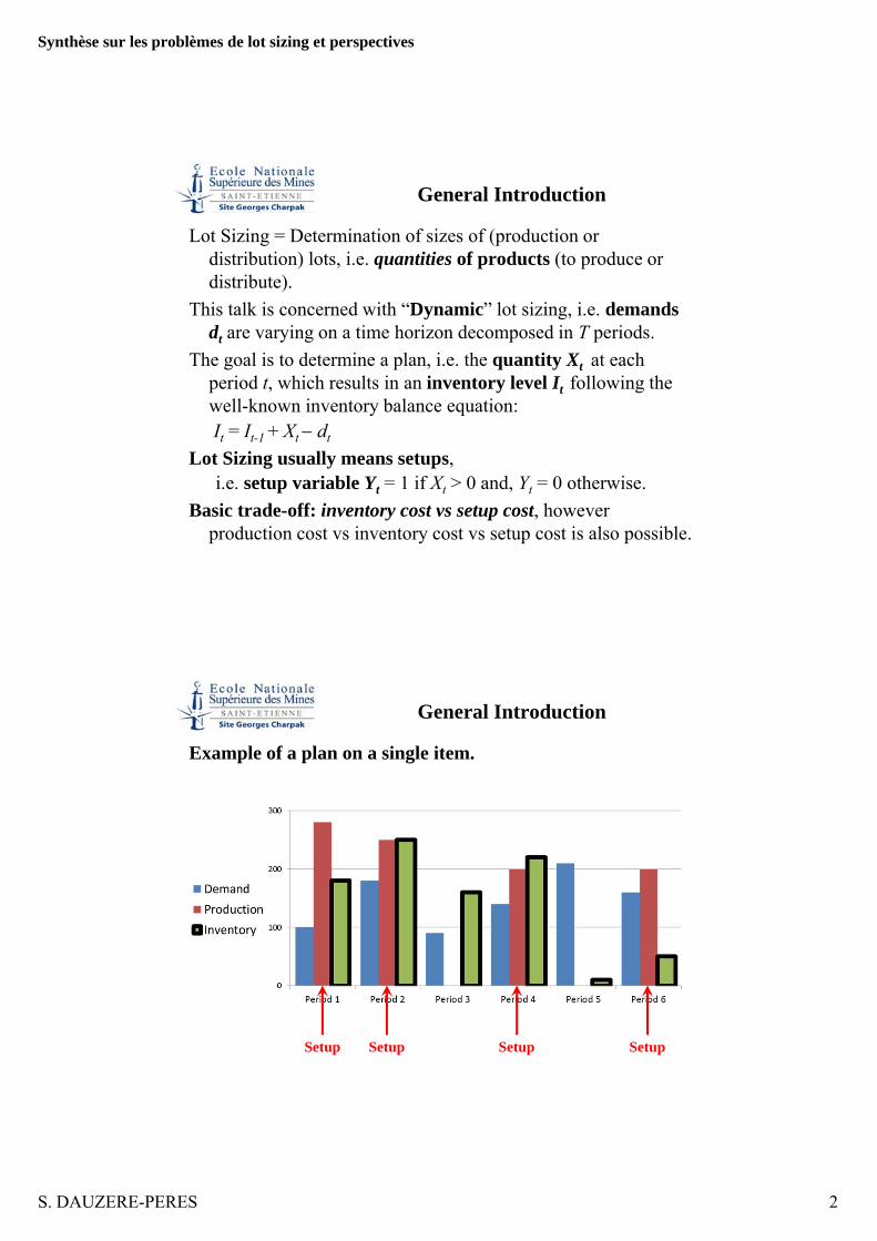
The goal is to determine a plan, i.e. the quantity Xt at each period t, which results in an inventory level It following the well-known inventory balance equation:It = It-1 + Xt − dt
Lot Sizing usually means setups, i.e. setup variable Yt = 1 if Xt > 0 and, Yt = 0 otherwise.
Basic trade-off: inventory cost vs setup cost, however production cost vs inventory cost vs setup cost is also possible.
General Introduction
Example of a plan on a single item.
Setup Setup Setup Setup

Synthèse sur les problèmes de lot sizing et perspectives
S. DAUZERE-PERES 3
General IntroductionModeling Setups
Setup timeProduction time
Time
“Extra big” time buckets:Time
Big time buckets:Time
Small time buckets:
Focus of this talk
General IntroductionModeling Setups
• In big time bucket models, there is one setup for each period in which the product is produced.
• Classical big time bucket models:– The Uncapacitated Lot-Sizing Problem (ULSP)
(Wagner-Whitin problem)– The Capacitated Lot-Sizing Problem (CLSP)
Time
Big time buckets:

Synthèse sur les problèmes de lot sizing et perspectives
S. DAUZERE-PERES 4
General IntroductionModeling Setups
• In multi-item production, a setup can sometimes be saved by letting the same product produced last in a given period to be produced first in the next period (production carryovers):
• Most big time bucket models do not take into account carryovers and, in such cases, small time bucket models may be better suited.
• However, Aras and Swanson [1982] proposed a modification so that production carryovers can also be handled by big time bucket models.
Time
General IntroductionModeling Setups
• When time buckets are small, there is only one setup even if a production lot lasts for several periods→Means of considering scheduling decisions in lot-sizing models
• Some small time bucket models:– The Discrete Lot-sizing and Scheduling Problem (DLSP),
→ See presentation of C. Gicquel,– The Continuous Setup Lot-sizing Problem (CSLP),– The Proportional Lot-sizing and Scheduling Problem (PLSP),– The General Lot-sizing and Scheduling Problem (GLSP).
Time
Small time buckets:

Synthèse sur les problèmes de lot sizing et perspectives
S. DAUZERE-PERES 5
General IntroductionModeling Setups
• Time buckets are so big that each individual setup is not important for the total production capacity; there will normally be several setups for each product in the period.
• Setups are therefore not considered at all (“aggregate production planning”), and a pure LP model can be used.
• “Average setup time” is either deducted from the total capacity, or production time per unit is increased in order to compensate for the setup time.
Time
“Extra big” time buckets:
General Introduction
Lot-Sizing problems are useful in production and distribution, where many practical problems can be found.
The study of lot-sizing problems has been driven by the development of APS (Advanced Planning Systems).

Synthèse sur les problèmes de lot sizing et perspectives
S. DAUZERE-PERES 6
General Introduction
Renewal from the mid-2000’s, illustrated by the success of the International Workshop on Lot Sizing (IWLS) started in Gardanne in 2010.
General Introduction

Synthèse sur les problèmes de lot sizing et perspectives
S. DAUZERE-PERES 7
Problem modelingUncapacitated Lot-Sizing Problem (USLP)
• Decision variables:Yt = 1 if production (setup) in period t, = 0 otherwiseXt = Production quantity in period tIt = Inventory at the end of period t
• Parameters:dt = Demand in period tvt = Variable production cost per unit in period tst = Setup cost in period tct = Inventory holding cost per unit on stock at the end of period t
Problem modelingUncapacitated Lot-Sizing Problem (USLP)
Min ( )∑=
++T
ttttttt IcXvYs
1
subject to : tttt dIIX =−+ −1 t∀ ttt YMX ≤ t∀ 0, ≥tt IX t∀ { }1,0=tY t∀
Where Mt is an upper bound of Xt, e.g. Mt = dt + … + dT.

Synthèse sur les problèmes de lot sizing et perspectives
S. DAUZERE-PERES 8
Problem modelingUncapacitated Lot-Sizing Problem (USLP)
Analysis of the Linear Relaxation, i.e. when Y ≥ 0.What happens to Yt in an optimal solution?→ Yt will be equal to Xt / Mt (as long as setup cost st > 0),→ If Mt is much larger than Xt, then Yt will be close to zero,→ Optimal value of LP relaxation will be much lower than
optimal value of original problem.→ Efficiency of standard solvers depend on choice of Mt. → Various valid inequalities have been proposed.
Problem modelingUncapacitated Lot-Sizing Problem (USLP)
Valid inequality (l, S). (Barany, Van Roy and Wolsey, 1984)By definition, if there is a production in period t (i.e. Xt > 0 and Yt = 1), then dt is produced in t. → The following inequality is valid: Xt ≤ dt Yt + It. This inequality can be generalized to two periods:
Xt + Xt+1 ≤ (dt + dt+1)Yt + dt+1 Yt+1 + It+1
and to any number of periods. (l, S) inequalities (exponential number) can be used to fully describe the convex hull of the USLP.
∑ ∑∑∈ =∈
+≤Sl
tl
t
lkk
Sll IYdX )( t∀ , { }tS ,,1K⊆∀

Synthèse sur les problèmes de lot sizing et perspectives
S. DAUZERE-PERES 9
Problem modelingSingle-item Lot-Sizing Problems
Uncapacitated can be solved in O(T2) (Wagner and Whitin, 1958) and O(T logT) (Federgruen and Tzur, 1991) (Wagelmans, van Hoesel and Kolen, 1992) (Aggarwal and Park, 1993).Capacited single-item lot sizing:Notation α / β / γ / δ (Bitran and Yanasse, 1982)
α, β, γ, δ = Z (Zero), C (Constant), NI (Non Increasing), ND (Non Decreasing), G (General)
Setup cost
Holding cost
CapacityProduction cost
Problem modelingSingle-item Lot-Sizing Problems
Capacited single-item lot sizing:The general case is NP-hard.Polynomial cases:
Problem Complexity References
NI/G/NI/ND O(T4)O(T2)
Bitran and Yanasse (1982)Chung and Lin (1988)
NI/G/NI/C O(T3) Bitran and Yanasse (1982)
C/Z/C/G O(TlogT) Bitran and Yanasse (1982)
ND/Z/ND/NI O(T) Bitran and Yanasse (1982)
G/G/G/C O(T4)O(T3)
Florian and Klein (1971)Van Hoesel and Wagelmans (1996)

Synthèse sur les problèmes de lot sizing et perspectives
S. DAUZERE-PERES 10
Problem modelingMulti-item Lot-Sizing Problem (CLSP)
• Decision variables:Yit = 1 if production (setup) of item i in period t, = 0 otherwiseXit = Production quantity of item i in period tIit = Inventory of item i at the end of period t
• Parameters:dit = Demand for item i in period tvit = Variable production cost per unit of item i in period tsit = Setup cost for item i in period tcit = Inventory holding cost per unit of item i on stock at the end of
period tpit = Production time per unit of item i in period tht = Available time for production in period t
Problem modelingMulti-item Lot-Sizing Problem (CLSP)
CLSP is NP hard in the strong sense (Chen and Thizy, 1990).
Min ( )∑∑==
++T
titititititit
N
iIcXvYs
11
subject to : itititit dIIX =−+ −1 ti ∀∀ ,
∑=
≤N
ititit hXp
1
t∀
ititit YMX ≤ ti ∀∀ , 0, ≥itit IX ti ∀∀ , { }1,0∈itY ti ∀∀ ,

Synthèse sur les problèmes de lot sizing et perspectives
S. DAUZERE-PERES 11
Problem modelingCLSP with setup times
New parameter: τit = Fixed setup time of item i in period t
With setup times, checking that a feasible solution exists is already NP-Complete (Trigeiro, Thomas and McClain, 1989).
Min ( )∑∑==
++T
titititititit
N
iIcXvYs
11
itititit dIIX =−+ −1 ti ∀∀ ,
t
N
iitit
N
iitit hYXp ≤+∑∑
== 11τ t∀
ititit YMX ≤ ti ∀∀ , 0, ≥itit IX ti ∀∀ , { }1,0∈itY ti ∀∀ ,
Problem modelingCLSP with backlog
New variable: Bit = Backlog of item i at the end of period tNew parameter: bit = Variable cost per unit of i backordered in t
Single-item case solved in O(T2) with an extension of Wagner-Whitin algorithm (Zangwill, 1969).
Min ( )∑∑==
+++T
titititititititit
N
iBbIcXvYs
11
itititititit dBIBIX =−−−+ −− )()( 11 ti ∀∀ ,
t
N
iitit
N
iitit hYXp ≤+∑∑
== 11
τ t∀
ititit YMX ≤ ti ∀∀ , 0,, ≥ititit BIX ti ∀∀ , { }1,0∈itY ti ∀∀ ,

Synthèse sur les problèmes de lot sizing et perspectives
S. DAUZERE-PERES 12
Problem modelingCLSP with lost sales
New variable: Lit = Lost sale of item i at the end of period tNew parameter: lit = Variable cost per unit of i lost in t
Single-item case solved in O(T2) (Aksen, Altinkemer and Chand, 2003).
Min ( )∑∑==
+++T
titititititititit
N
iLlIcXvYs
11
ititititit dLIIX =−−+ − )(1 ti ∀∀ ,
t
N
iitit
N
iitit hYXp ≤+∑∑
== 11τ t∀
ititit YMX ≤ ti ∀∀ , 0,, ≥ititit LIX ti ∀∀ , { }1,0∈itY ti ∀∀ ,
Problem modelingCLSP with lost sales
New variable: Lit = Lost sale of item i at the end of period tNew parameter: lit = Variable cost per unit of i lost in t
Lagrangian based metaheuristics proposed for the multi-item case (Absi, Detienne and D.-P., 2013).
Min ( )∑∑==
+++T
titititititititit
N
i
LlIcXvYs11
ititititit dLIIX =−−+ − )(1 ti ∀∀ ,
t
N
iitit
N
iitit hYXp ≤+∑∑
== 11τ t∀
ititit YMX ≤ ti ∀∀ , 0,, ≥ititit LIX ti ∀∀ , { }1,0∈itY ti ∀∀ ,

Synthèse sur les problèmes de lot sizing et perspectives
S. DAUZERE-PERES 13
Classifications
Lot Sizing
Single Level
Multi Level
Single Product
Multi product
Backlogging
Perishable products
Remanufacturing
With capacity
No capacity
Zangwill (1969)
Hsu (2000)
Golany, Yan, Yu (2001)
Florian et Klein (1971)
Wagner et Whitin (1958)State of the artBrahimi et al. 2006
Multi product
Time windows on demands
Lee, Cetinkaya, Wagelmans (2001)
Classifications
Lot Sizing
Single Level
Multi Level
Single Product
Multi product
Multi product
Backlogging
Perishable products
Remanufacturing
Capacity
Setup times
Joint setups
Manne (1958)
Trigeiro et al. (1989)
Suerie et Stadtler (2003)
Millar et Yang (1993)
Friedman et Hoch (1978)
Richter et Sonbrutzki (2000)
State of the artKarimi et al. 2003

Synthèse sur les problèmes de lot sizing et perspectives
S. DAUZERE-PERES 14
Tighter formulations
Multiple formulations were proposed for the single-item and multi-item problems to improve on the linear relaxation of the aggregate formulation, and get better solutions with a standard solver.
Disaggregate formulationUncapacitated Lot-Sizing Problem (ULSP)
Also called facility location model (Krarup and Bilde, 1977).• New variable: Ztk = quantity produced in period t to cover
demand in period k.• New parameter: cdtk = variable production cost plus inventory
cost for producing one unit in period t and storing it until period k, i.e.
∑−
=−−++ +=++++++=
1
1221 ...k
tuutkktttttk cvcccccvcd

Synthèse sur les problèmes de lot sizing et perspectives
S. DAUZERE-PERES 15
Disaggregate formulationUncapacitated Lot-Sizing Problem (ULSP)
Min ∑=
T
tttYs
1+∑∑
= =
T
t
T
tktktk Zcd
1
k
k
ttk dZ =∑
=1 k∀
tktk YdZ ≤ tkt ≥∀∀ , 0≥tkZ tkt ≥∀∀ , { }1,0=tY t∀
Disaggregate formulationCapacited Lot-Sizing Problem (CLSP)
• New variable: Zitk = quantity of item i produced in period t to cover demand in period k.
• New parameter: cditk = variable production cost plus inventory cost for producing one unit of item i in period t and storing it until period k, i.e.
∑−
=−−++ +=++++++=
1
1221 ...k
tuiuitikikitititititk cvcccccvcd

Synthèse sur les problèmes de lot sizing et perspectives
S. DAUZERE-PERES 16
Disaggregate formulationCapacited Lot-Sizing Problem (CLSP)
Min ∑∑= =
N
i
T
tititYs
1 1+∑∑∑
= = =
N
i
T
t
T
tkitkitk Zcd
1 1
ikk
titk dZ =∑
=1 ki ∀∀ ,
∑ ∑∑= ==
≤+N
it
N
iitit
T
tkitkit hYZp
1 1τ t∀
itititk YdZ ≤ tkti ≥∀∀∀ ,, 0≥itkZ tkti ≥∀∀∀ ,,
{ }1,0∈itY ti ∀∀ ,
Shortest Path formulationCapacited Lot-Sizing Problem (CLSP)
(Eppen and Martin, 1987)• New variable: ZZitk = fraction of total demand of item i for
periods t through k that is produced in period t (∈ [0,1]).• New parameter: ccitk = variable production cost plus
inventory cost for producing in period t and storing the demands from periods t to k of item i, i.e.
ikik
k
tlilit
k
tlilit
k
tlilititk dcdcdcdvcc 1
21
1... −
+=+
+==
++++= ∑∑∑
∑∑∑+=
−
==
+=k
ulil
k
tuiu
k
tlilititk dcdvcc
1
1

Synthèse sur les problèmes de lot sizing et perspectives
S. DAUZERE-PERES 17
Shortest Path formulationCapacited Lot-Sizing Problem (CLSP)
Min ∑∑= =
N
i
T
tititYs
1 1+∑∑∑
= = =
N
i
T
t
T
tkitkitk ZZcc
1 1
11
1 =∑=
T
kkiZZ i∀
∑∑=
−
=− =
T
tkitk
t
lilt ZZ
1
11 2, ≥∀∀ ti
∑ ∑∑ ∑= == =
≤+N
it
N
iitit
T
tkitk
k
tlilit hYZZdp
1 1
)( τ t∀
it
T
tkitk YZZ ≤∑
=
ti ∀∀ ,
0≥itkZZ tkti ≥∀∀∀ ,, { }1,0∈itY ti ∀∀ ,
Solving the single-item caseWagner-Whitin algorithm
In the uncapacitated case, the Zero Inventory Order (ZIO) property is satisfied, i.e. plans where “It-1 Xt = 0 ∀t” are dominant
→ Order quantities cover an integer number of periods in dominant plans,
→ There is an optimal solution which is a dominant plan,→Wagner Whitin algorithm uses ZIO property,→ ZIO property often checked when analyzing a new lot-sizing
problem.

Synthèse sur les problèmes de lot sizing et perspectives
S. DAUZERE-PERES 18
Solving the single-item caseWagner-Whitin algorithm
Example.setup cost st = 15 ∀ tinventory cost ct = 1 ∀ tdemand dt = (4, 8, 6, 7)The dominant plans are:
( 4, 8, 6, 7)( 4, 8, 13, 0)( 4, 14, 0, 7)( 4, 21, 0, 0)(12, 0, 6, 7) (12, 0, 13, 0)(18, 0, 0, 7) (25, 0, 0, 0)
Solving the single-item caseWagner-Whitin algorithm
In general, there will be 2(T-1) dominant plans.By using dynamic programming, the Wagner-Whitin algorithm
further reduces the complexity of the search to T(T+1)/2, i.e. O(T2) (Wagner and Whitin, 1958).

Synthèse sur les problèmes de lot sizing et perspectives
S. DAUZERE-PERES 19
Solving the single-item caseWagner-Whitin algorithm
Example.setup cost st = 15 ∀ tinventory cost ct = 1 ∀ tdemand dt = (4, 8, 6, 7)
Optimal solution.X1 = 12 X2 = 0 X3 = 13 X4 = 0I1 = 8 I2 = 0 I3 = 7 I4 = 0Y1 = 1 Y2 = 0 Y3 = 1 Y4 = 0
Setup costs: 30Inventory costs: 15Total costs: 45
Solving the single-item caseWagner-Whitin algorithm
In general, there will be 2(T-1) dominant plans.By using dynamic programming, the Wagner-Whitin algorithm
further reduces the complexity of the search to T(T+1)/2, i.e. O(T2) (Wagner and Whitin, 1958).
More recently, the complexity has been reduced to O(T log(T)) (Federgruen and Tzur, 1991), (Wagelmans Van Hoesel and Kolen, 1992) , (Aggarwal and Park, 1993).
Synthèse sur les problèmes de lot sizing et perspectives
S. DAUZERE-PERES 20
Solving the single-item caseHeuristics
Heuristics for single-item problems can be useful to solve more complex problems and to develop heuristics for multi-item problems:
• Part-Period BalancingAims at balancing total ordering cost and total holding cost
• Silver and Meal heuristicAims at minimizing the cost per period
• Least Unit CostAims at minimizing the total cost per unit of product
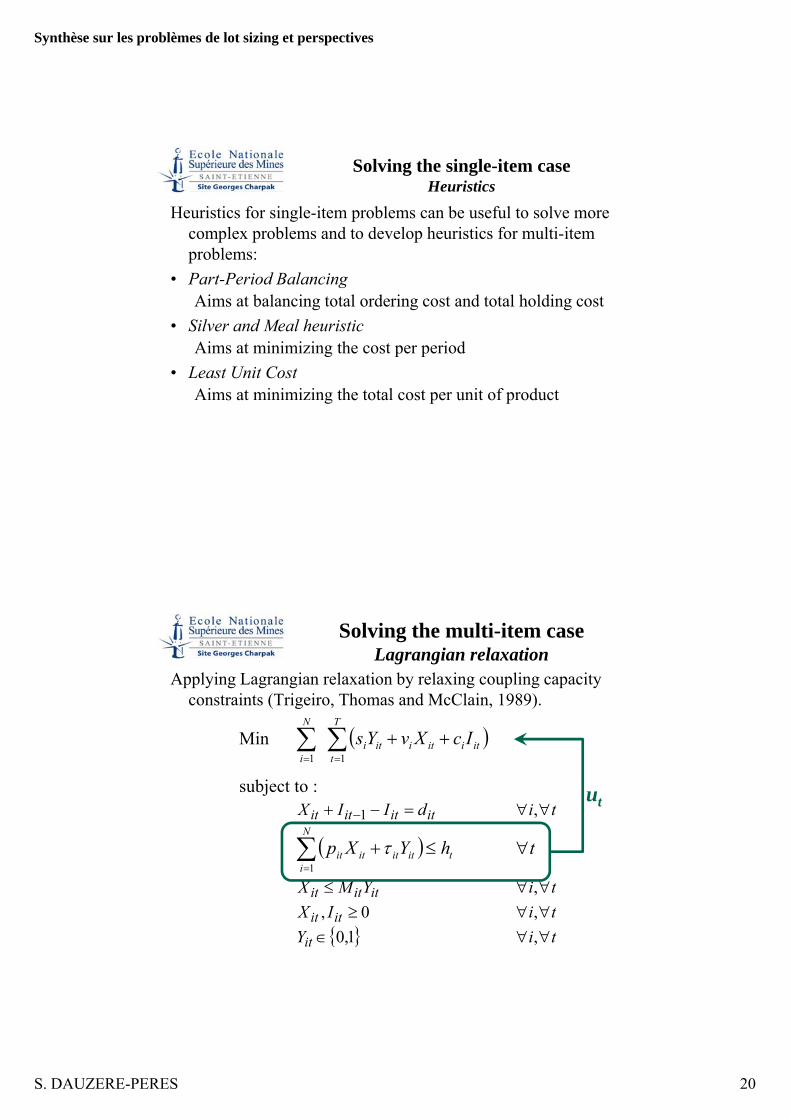
Solving the multi-item caseLagrangian relaxation
Applying Lagrangian relaxation by relaxing coupling capacity constraints (Trigeiro, Thomas and McClain, 1989).
Min ( )∑∑==
++T
titiitiiti
N
i
IcXvYs11
subject to : itititit dIIX =−+ −1 ti ∀∀ ,
( )∑=
≤+N
ititititit hYXp
1
τ t∀
ititit YMX ≤ ti ∀∀ , 0, ≥itit IX ti ∀∀ , { }1,0∈itY ti ∀∀ ,
ut

Synthèse sur les problèmes de lot sizing et perspectives
S. DAUZERE-PERES 21
Solving the multi-item caseLagrangian relaxation
Lagrangian relaxation model.
→ Uncapacitated single-item problems (Wagner Whitin problem) can be solved separately in O(T logT).
Min ( ) ∑∑∑===
−++++T
ttt
T
titiitittiititti
N
i
huIcXpuvYus111
)()( τ
subject to : itititit dIIX =−+ −1 ti ∀∀ , ititit YMX ≤ ti ∀∀ , 0, ≥itit IX ti ∀∀ , { }1,0∈itY ti ∀∀ ,
Solving the multi-item caseLagrangian relaxation
Lagrangian relaxation model.
Note that Lagrangian production and setup costs are period dependent.
Min ( ) ∑∑∑===
−++++T
ttt
T
titiitittiititti
N
i
huIcXpuvYus111
)()( τ
subject to : itititit dIIX =−+ −1 ti ∀∀ , ititit YMX ≤ ti ∀∀ , 0, ≥itit IX ti ∀∀ , { }1,0∈itY ti ∀∀ ,

Synthèse sur les problèmes de lot sizing et perspectives
S. DAUZERE-PERES 22
Solving the multi-item caseLagrangian relaxation heuristic
1. Solve Lagrangian relaxation model to determine optimal values of variables Xit and Yit.
2. Use solution to compute Lagrangian lower bound of optimal solution.
3. Use values of variables obtained in Step 1 to determine a feasible solution of original problem (smoothing heuristic).Update upper bound (best feasible solution).
4. Update Lagrange multipliers (subgradient), so that relaxed capacity constraints not satisfied have more chances to be satisfied at next iteration.Go to Step 1 if none of the stopping criteria is satisfied (duality gap
small enough, step size, number of iterations, …).
Solving the multi-item caseSmoothing (feasibility) heuristic
The goal is to ensure feasibility of the plan through forward and backward passes.
Forward pass.

Synthèse sur les problèmes de lot sizing et perspectives
S. DAUZERE-PERES 23
Solving the multi-item caseSmoothing (feasibility) heuristic
Backward pass.
Solving the multi-item caseSmoothing (feasibility) heuristic
Leads to a feasible plan.
Feasibility is not guaranteed (in particular with setup times).→ Smoothing heuristics can be applied after any heuristic
building initial unfeasible solutions.

Synthèse sur les problèmes de lot sizing et perspectives
S. DAUZERE-PERES 24
Min ∑∑= =
N
i
T
tititYs
1 1+∑∑∑
= = =
N
i
T
t
T
tkitkitk ZZcc
1 1
11
1 =∑=
T
kkiZZ i∀
∑∑−
=−
=
=1
11
t
lilt
T
tkitk ZZ 2, ≥∀∀ ti
∑ ∑∑ ∑= == =
≤+N
it
N
iitit
T
tkitk
k
tlilit hYZZdp
1 1)( τ t∀
it
T
tkitk YZZ ≤∑
=
ti ∀∀ ,
0≥itkZZ tkti ≥∀∀∀ ,, { }1,0∈itY ti ∀∀ ,
Capacited Lot-Sizing Problem (CLSP)Comparing lower bounds
OPT
RLag(SP)
ut
vit
Min ( )∑∑==
++T
titititititit
N
iIcXvYs
11
itititit dIIX =−+ −1 ti ∀∀ ,
∑=
≤N
ititit cXp
1 t∀
ititit YMX ≤ ti ∀∀ , 0, ≥itit IX ti ∀∀ , { }1,0∈itY ti ∀∀ ,
Capacited Lot-Sizing Problem (CLSP)Comparing lower bounds
OPT
RLag(SP)
RLag(AGG)
ut

Synthèse sur les problèmes de lot sizing et perspectives
S. DAUZERE-PERES 25
Min ∑∑= =
N
i
T
tititYs
1 1+∑∑∑
= = =
N
i
T
t
T
tkitkitk ZZcc
1 1
11
1 =∑=
T
kkiZZ i∀
∑∑−
=−
=
=1
11
t
lilt
T
tkitk ZZ 2, ≥∀∀ ti
∑ ∑∑ ∑= == =
≤+N
it
N
iitit
T
tkitk
k
tlilit hYZZdp
1 1)( τ t∀
it
T
tkitk YZZ ≤∑
=
ti ∀∀ ,
0≥itkZZ tkti ≥∀∀∀ ,, { }1,0∈itY ti ∀∀ ,
Capacited Lot-Sizing Problem (CLSP)Comparing lower bounds
OPT
RLag(SP)
RLag(AGG)
RLag(SP)
ut
Min ∑∑= =
N
i
T
tititYs
1 1+∑∑∑
= = =
N
i
T
t
T
tkitkitk ZZcc
1 1
11
1 =∑=
T
kkiZZ i∀
∑∑−
=−
=
=1
11
t
lilt
T
tkitk ZZ 2, ≥∀∀ ti
∑ ∑∑ ∑= == =
≤+N
it
N
iitit
T
tkitk
k
tlilit hYZZdp
1 1)( τ t∀
it
T
tkitk YZZ ≤∑
=
ti ∀∀ ,
0≥itkZZ tkti ≥∀∀∀ ,, { }1,0∈itY ti ∀∀ ,
Capacited Lot-Sizing Problem (CLSP)Comparing lower bounds
OPT
RLag(SP)
RLag(AGG)
RLag(SP)
RL(SP)

Synthèse sur les problèmes de lot sizing et perspectives
S. DAUZERE-PERES 26
Min ( )∑∑==
++T
titititititit
N
iIcXvYs
11
itititit dIIX =−+ −1 ti ∀∀ ,
∑=
≤N
ititit cXp
1 t∀
ititit YMX ≤ ti ∀∀ , 0, ≥itit IX ti ∀∀ , { }1,0∈itY ti ∀∀ ,
Capacited Lot-Sizing Problem (CLSP)Comparing lower bounds
OPT
RLag(SP)
RLag(AGG)
RLag(SP)
RLag(AGG)
RL(SP)
vit
Min ( )∑∑==
++T
titititititit
N
iIcXvYs
11
itititit dIIX =−+ −1 ti ∀∀ ,
∑=
≤N
ititit cXp
1 t∀
ititit YMX ≤ ti ∀∀ , 0, ≥itit IX ti ∀∀ , { }1,0∈itY ti ∀∀ ,
Capacited Lot-Sizing Problem (CLSP)Comparing lower bounds
OPT
RLag(SP)
RL(AGG)
RLag(AGG)
RLag(SP)
RLag(AGG)
RL(SP)
Synthèse sur les problèmes de lot sizing et perspectives
S. DAUZERE-PERES 27
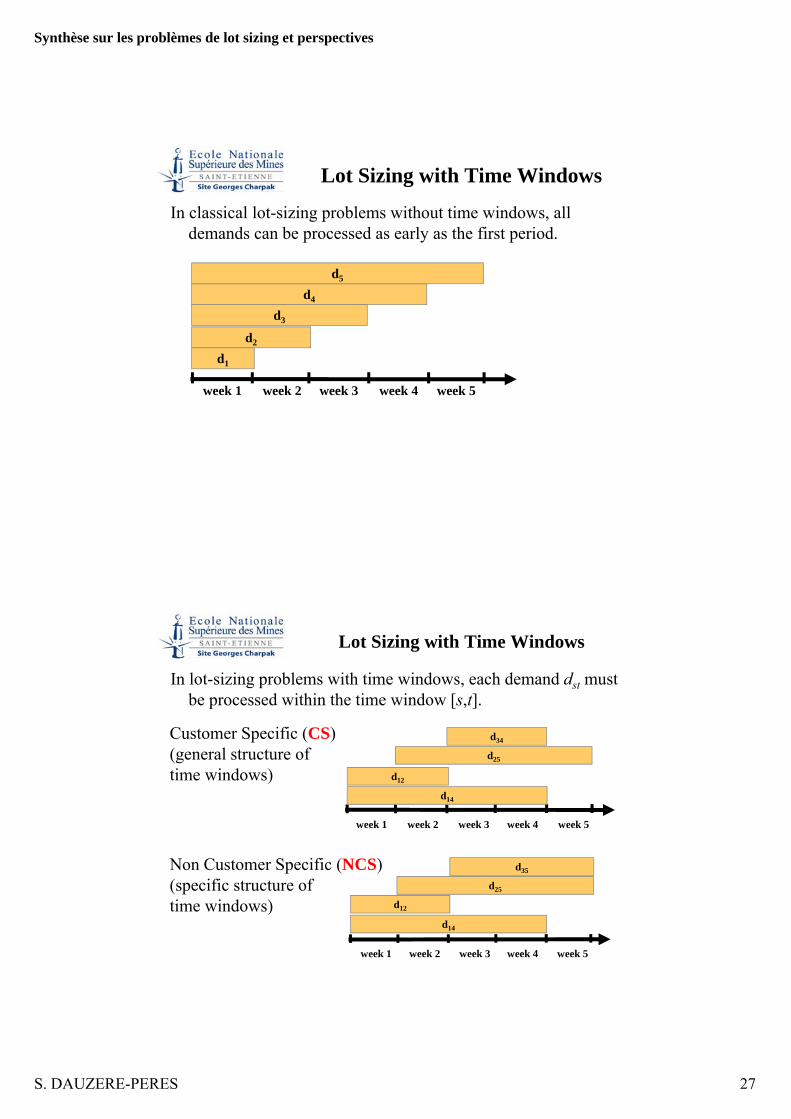
Lot Sizing with Time Windows
In classical lot-sizing problems without time windows, all demands can be processed as early as the first period.
d4
d5
week 1 week 2 week 3 week 4 week 5
d3
d2
d1
Lot Sizing with Time Windows
In lot-sizing problems with time windows, each demand dst must be processed within the time window [s,t].
week 1 week 2 week 3 week 4 week 5
d14
d34
d12
d25
Customer Specific (CS)(general structure of time windows)
d14
d25
d35
d12
week 1 week 2 week 3 week 4 week 5
Non Customer Specific (NCS)(specific structure of time windows)

Synthèse sur les problèmes de lot sizing et perspectives
S. DAUZERE-PERES 28
Lot Sizing with Time Windows
Complexity for Customer Specific (CS) single-item problem• Solved using dynamic programming in exponential time in
(D.-P., Brahimi, Najid and Nordli, 2002).• Solved in O(T5) in (Huang, 2007) Complexity for Non Customer Specific (NCS) single-item problem• Exponential time algorithm for CS problem runs in O(T4) for
NCS problem (D.-P., Brahimi, Najid and Nordli, 2002).• Improved to O(T2) in (Wolsey, 2006).• Generalization to early productions, backlogs and lost sales
solved in O(T2) in (Absi, Kedad-Sidhoum and D.-P., 2011).Lagrangian relaxation heuristics proposed in (Brahimi, D.-P. and Najid, 2006) for CS and NCS multi-item problems.
Green Lot SizingLot Sizing with carbon emissions
• Recent research on lot sizing is concerned with considering new environmental constraints.
• A global carbon emission constraint is considered in (Benjaafar, Li and Daskin, 2010).→ Acts as a capacity constraint.
• Four types of carbon emission constraints are proposed and analyzed in the single-item case in (Absi, D.-P., Kedad-Sidhoum, Penz and Rapine, 2013). → Theses constraints do not limit lot sizes, but limit the
carbon emission per unit of product.→ See presentation of S. Kedad-Sidhoum.

Synthèse sur les problèmes de lot sizing et perspectives
S. DAUZERE-PERES 29
Multi-Level (Multi-Stage) Lot Sizing
Independent demands (for end products) and dependent demands
End product
Subassembly X Subassembly Y
(2) (1)
Part A Part B
(3) (5) (3)
Part C
(2)
Component D Component F
(10) (4)
Component E
(1) (1)
Multi-Level Lot Sizing
New parameter gij: Number of items i necessary to produce one unit of item j (gozinto factor).
New inventory balance equation becomes a coupling constraint.
Min ( )∑∑==
++T
titititititit
N
iIcXvYs
11
∑=
− +=−+N
jjtijitititit XgdIIX
11 ti ∀∀ ,
∑=
≤N
ititit hXp
1 t∀
ititit YMX ≤ ti ∀∀ , 0, ≥itit IX ti ∀∀ , { }1,0∈itY ti ∀∀ ,
Dependent demandIndependent demand

Synthèse sur les problèmes de lot sizing et perspectives
S. DAUZERE-PERES 30
Multi-Level Lot Sizing
See presentation of J.-P. Casal (FuturMaster).Various approaches have been proposed: • Lagrangian relaxation (Tempelmeier and Derstroff, 1996),• MIP-based heuristics (used in general for complex lot-sizing
problems).
MIP-based heuristics for Lot Sizing
• Iterative approaches.• Solve at each stage a reduced mixed integer problem.• By reducing the number of binary variables and the number of
constraints.• Various decompositions can be used::
– An horizon-oriented decomposition,– A product-oriented decomposition,– A resource-oriented decomposition,– A process-oriented decomposition, etc.

Synthèse sur les problèmes de lot sizing et perspectives
S. DAUZERE-PERES 31
MIP-based heuristics for Lot Sizing
Several variants:• Relax-and-Fix, Fix-and-Relax (Kelly 2002, Clark 2003, Mercé and
Fontan 2003, , Stadtler 2003, Pochet and Van Vyve 2004, Absi and kedad-Sidhoum 2007, Federgruen et al. 2007, Seeanner et al. 2013),
• Fix-and-Optimize (Sahling et al. 2009, S Helber, F Sahling 2010, Lang and Shen 2011, James and Almada-Lobo 2011).
MIP-based heuristics for Lot Sizing
Example of an horizon-oriented decomposition (Absi and Kedad-Sidhoum 2007) – Relax-and-Fix
Step 2Step 3Step 1
Frozen window
Decision window
Approximation window
σ: Overlapping sectionδ: Size of decision windows
0 T

Synthèse sur les problèmes de lot sizing et perspectives
S. DAUZERE-PERES 32
Integrating Lot-Sizing decisions and other types of decisions
More and more researchers are studying the integration of lot-sizing decisions with decisions taken at other levels or other stages in the supply chain.
Integrating Lot-Sizing decisions and other types of decisions
Plant design
Prod. planning
Prod. scheduling
Productionsystem
Storage capacity
Capacity planning
Storage scheduling
Storagesystem
Network design
Transport planning
Vehicle routing
Transportsystem
Possible decision processes in a supply chain
Lot Sizing

Synthèse sur les problèmes de lot sizing et perspectives
S. DAUZERE-PERES 33
Integrating Lot-Sizing decisions and other types of decisions
Variables at different levels/stages are often of different nature, i.e. no longer pure continuous or integer optimization problems →Makes the integration particularly complex and changes
the nature of the problems.Objectives at different levels/stages may be of different nature, e.g. cost minimization vs. time criteria.
Integrating Lot-Sizing and Cutting-Stock decisions
Column Generation approaches are used in (Nonås and Thorstenson, 2000) and (Nonås and Thorstenson, 2008) to solve a combined lot-sizing and cutting-stock problem.
(Gramani and França, 2006) analyzes the trade-off in industrial problems, where trim loss, storage and setup costs are minimized. The problem is solved using a network shortest path formulation. (Gramani, França and Arenales, 2009) proposes a Lagragian relaxation heuristic.Heuristics are also proposed in (Poltroniere, Poldi, Toledo and Arenales, 2008)

Synthèse sur les problèmes de lot sizing et perspectives
S. DAUZERE-PERES 34
Integrating Lot-Sizing and Scheduling decisions
Plant design
Prod. planning
Prod. scheduling
Productionsystem
Storage capacity
Capacity planning
Storage scheduling
Storagesystem
Network design
Transport planning
Vehicle routing
Transportsystem
Integrating Lot-Sizing and Scheduling decisions
Strategic level
Production system
Tactical level
Operational level
Production Plan
Schedules
Decisions
Feedback
Information
Horizon, demands, capacity constraints, ...
Routings, processingtimes, ...

Synthèse sur les problèmes de lot sizing et perspectives
S. DAUZERE-PERES 35
Integrating Lot-Sizing and Scheduling decisions
Planning and scheduling can hardly be treated simultaneously
When and How(discrete variables)
How much(continuous variables)
Scheduling
Production planning(Lot Sizing)
Aggregate (necessary) capacity constraints are used→ No actual schedule to satisfy the plan→ Delays, work-in-process inventories
Integrating Lot-Sizing and Scheduling decisions
• Integration of production planning and detailed scheduling (Lasserre 1989, D-P. and Lasserre 1994 and 2002)
– Multi-item lot-sizing problem,– Combined with job-shop scheduling problem.
• Scientific challenges:– Multi-item lot-sizing problem with complex capacity
constraints,– Or job-shop scheduling problem where processing times are
variables.• Practical challenges (e.g. Renault and “25% rule” in 1996).

Synthèse sur les problèmes de lot sizing et perspectives
S. DAUZERE-PERES 36
Integrating Lot-Sizing and Scheduling decisions – A simple example
Two products A and B
Three machines M1, M2 and M3
InputM1
pA,1 = 2 h/up
pB,1 = 3 h/upM2
pA,2 = 1 h/up
pB,2 = 1 h/upM3
pA,3 = 1 h/up
pB,3 = 2 h/up
Output
Length of a period: 60 h
Quantities to be produced: XA and XB
Integrating Lot-Sizing and Scheduling decisions – A simple example
InputM1
pA,1 = 2 h/up
pB,1 = 3 h/upM2
pA,2 = 1 h/up
pB,2 = 1 h/upM3
pA,3 = 1 h/up
pB,3 = 2 h/up
Output
Machine constraints:M1: 2 XA + 3 XB ≤ 60 M2: XA + XB ≤ 60M3: XA + 2 XB ≤ 60
→ XA = 10 and XB = 10 are feasible

Synthèse sur les problèmes de lot sizing et perspectives
S. DAUZERE-PERES 37
Integrating Lot-Sizing and Scheduling decisions – A simple example
Schedule of the operations in classical planning (M.R.P.)
Time
Product A
Product B
10 20 30 40 50 60
M1
M1
M2
M2
M3
M3
→ Operations are not sequenced
Integrating Lot-Sizing and Scheduling decisions – A simple example
Product A sequenced before product B
Time
M3
M2
10 20 30 40 50 60
A
B
70 80
M1 B
B
A
A

Synthèse sur les problèmes de lot sizing et perspectives
S. DAUZERE-PERES 38
Integrating Lot-Sizing and Scheduling decisions – A simple example
Product B sequenced before product A
Time
M3
M2
10 20 30 40 50 60
A
B
70 80
M1 B
B
A
A
Integrating Lot-Sizing and Scheduling decisions
Planning (Lot-Sizing) problem
Scheduling problem

Synthèse sur les problèmes de lot sizing et perspectives
S. DAUZERE-PERES 39
Integrating Lot-Sizing and Scheduling decisions
• A two-level iterative procedure has been used to solve the problem (Lasserre 1989, D.-P. and Lasserre 1994, 2002, Roux, D.-P. and Lasserre 1999)Comparison between feasible production plans obtained with aggregate
model and integrated model with one-pass and iterative procedures
ProblemTotal inventory and backlog costs
Aggregate One-pass Iterative1 7538 5248 4347
2 17036 12638 122463 6318 3913 2651
4 2457 883 1335 3318 482 220
6 698 0 0
Integrating Lot-Sizing and Scheduling decisions
• A two-level iterative procedure has been used to solve the problem (Lasserre 1989, D.-P. and Lasserre 1994, 2002, Roux, D.-P. and Lasserre 1999)
• More recently an integrated approach has been proposed in (Wolosewicz, D.-P. and Aggoune, 2008)→ Pursued in PhD thesis of Edwin Gomez for multi-level lot-
sizing problems in a supply chain• Novel formulation based on graph representation of
scheduling problem, where each path corresponds to a capacity constraint.→ Exponential number of capacity constraints→ Lagrangian relaxation approach where violated paths
are inserted one by one with positive Lagrangian multiplier

Synthèse sur les problèmes de lot sizing et perspectives
S. DAUZERE-PERES 40
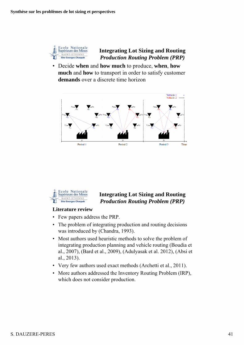
Integrating Lot Sizing and RoutingProduction Routing Problem (PRP)
• Integrated optimization of production, distribution and inventory decisions.
Plant design
Prod. planning
Prod. scheduling
Productionsystem
Storage capacity
Capacity planning
Storage scheduling
Storagesystem
Network design
Transport planning
Vehicle routing
Transportsystem
Integrating Lot Sizing and RoutingProduction Routing Problem (PRP)
• Integrated optimization of production, distribution and inventory decisions.
• The PRP simultaneously optimizes production, inventory and routing so that final demands of customers and inventory limits in production facility and retailers are satisfied, while minimizing all types of costs.
Synthèse sur les problèmes de lot sizing et perspectives
S. DAUZERE-PERES 41
• Decide when and how much to produce, when, how much and how to transport in order to satisfy customer demands over a discrete time horizon
Integrating Lot Sizing and RoutingProduction Routing Problem (PRP)
Literature review• Few papers address the PRP.• The problem of integrating production and routing decisions
was introduced by (Chandra, 1993).• Most authors used heuristic methods to solve the problem of
integrating production planning and vehicle routing (Boudia et al., 2007), (Bard et al., 2009), (Adulyasak et al. 2012), (Absi et al., 2013).
• Very few authors used exact methods (Archetti et al., 2011).• More authors addressed the Inventory Routing Problem (IRP),
which does not consider production.
Integrating Lot Sizing and RoutingProduction Routing Problem (PRP)

Synthèse sur les problèmes de lot sizing et perspectives
S. DAUZERE-PERES 42
Mathematical model• Minimize production, inventory and routing costs subject to:
– Inventory balance constraints for retailers and production facility,– Inventory capacity constraints for retailers and production
facility,– Production constraints,– Vehicle capacity constraints,– Routing constraints.
Integrating Lot Sizing and RoutingProduction Routing Problem (PRP)
Solution approach (Absi, Archetti, Feillet and D.-P. 2012)• Iterative two-phase approach.• Routing costs incurred when visiting a customer at a given
period are approximated and denoted SCit.→ Initial model can then be transformed into a lot-sizing
model that optimizes production and inventory levels.• Distribution costs only interfere with the lot-sizing model
through the setup costs SCit.• First phase is called Lot-sizing Problem (SCit).• Using the solution obtained in first phase, routing decisions are
taken in second phase, called Routing Problem (γvit). → Corresponds to solving the vehicle routing problem once
the γvit variables are fixed.
Integrating Lot Sizing and RoutingProduction Routing Problem (PRP)

Synthèse sur les problèmes de lot sizing et perspectives
S. DAUZERE-PERES 43
Solution approach (general scheme)
Diversification mechanism: SCit multiplied by coefficient (routelength) when customer i belongs to existing route at period t.
Integrating Lot Sizing and RoutingProduction Routing Problem (PRP)
Lot-sizing phase• Optimize production plan with approximated routing costs SCit
(setup costs),• Decide when (γvit) and how much to produce, when and how
much to transport in order to satisfy customer demands.
Integrating Lot Sizing and RoutingProduction Routing Problem (PRP)

Synthèse sur les problèmes de lot sizing et perspectives
S. DAUZERE-PERES 44
Routing phase• Decide how to transport goods in order to satisfy customers
and vehicles capacities (Vehicle Routing Problem).
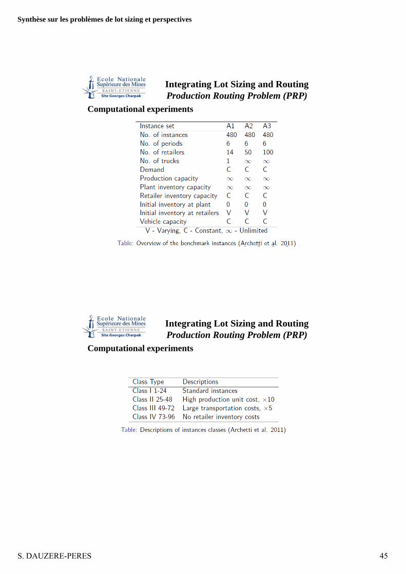
Integrating Lot Sizing and RoutingProduction Routing Problem (PRP)
Computational experiments• Stops after 20 iterations.• When solution not improved for 5 iterations, diversification
mechanism is used.• Comparison with heuristics of (Archetti et al., 2011) (H) and
(Adulyasak et al., 2012) (Op-ALNS).
Integrating Lot Sizing and RoutingProduction Routing Problem (PRP)
Synthèse sur les problèmes de lot sizing et perspectives
S. DAUZERE-PERES 45
Computational experiments
Integrating Lot Sizing and RoutingProduction Routing Problem (PRP)
Computational experiments
Integrating Lot Sizing and RoutingProduction Routing Problem (PRP)

Synthèse sur les problèmes de lot sizing et perspectives
S. DAUZERE-PERES 46
Computational results
Integrating Lot Sizing and RoutingProduction Routing Problem (PRP)
Classes IM H ALNS1 0,13% 2,13% 1,65%2 0,02% 0,30% 0,36%3 0,71% 3,43% 7,60%4 0,07% 0,88% 0,93%
All 0,23% 1,68% 2,64%
Average gaps to best solutions for 480
instances of set A1.
Integrating Lot Sizing and RoutingProduction Routing Problem (PRP)
Classes IM H ALNS1 0,04% 1,89% 0,98%2 0,02% 0,35% 0,14%3 0,26% 2,66% 2,66%4 0,04% 1,17% 0,13%
All 0,09% 1,52% 0,98%
Classes IM H ALNS1 0,06% 2,06% 0,82%2 0,19% 0,32% 0,29%3 0,23% 2,55% 2,53%4 0,18% 1,19% 0,26%
All 0,16% 1,53% 0,98%
Average gaps to best solutions for 480
instances of set A2.
Average gaps to best solutions for 480
instances of set A3.
Computational results

Synthèse sur les problèmes de lot sizing et perspectives
S. DAUZERE-PERES 47
Conclusions
• Lot sizing is (again…) an active field of research.• Numerous topics were not discussed in this presentation such
as: sequence-dependent setup times, joint setups, inventory bounds, stochastic lot sizing, various solution approaches (Column Generation, metaheuristics, …), …
• A lot of research remains to be done on the interface between lot sizing and other problems to define, in particular with industry, relevant combined problems.