SUPERSONIC BUSINESS JETDesign Space Exploration and Optimization

Josiah VanderMey

Hassan Bukhari

MIT 16.888/ESD.775

Overview

Problem Formulation

Motivation and Challenges

Objectives and Constraints

Model and Simulation

Model Overview and Description

Benchmarking and Validation

Optimization

Algorithms and tuning

Post Optimality Analysis

Multi-Objective and Tradeoff Analysis

Conclusions and Recommendations

2

Problem FormulationMotivation and Challenges

3

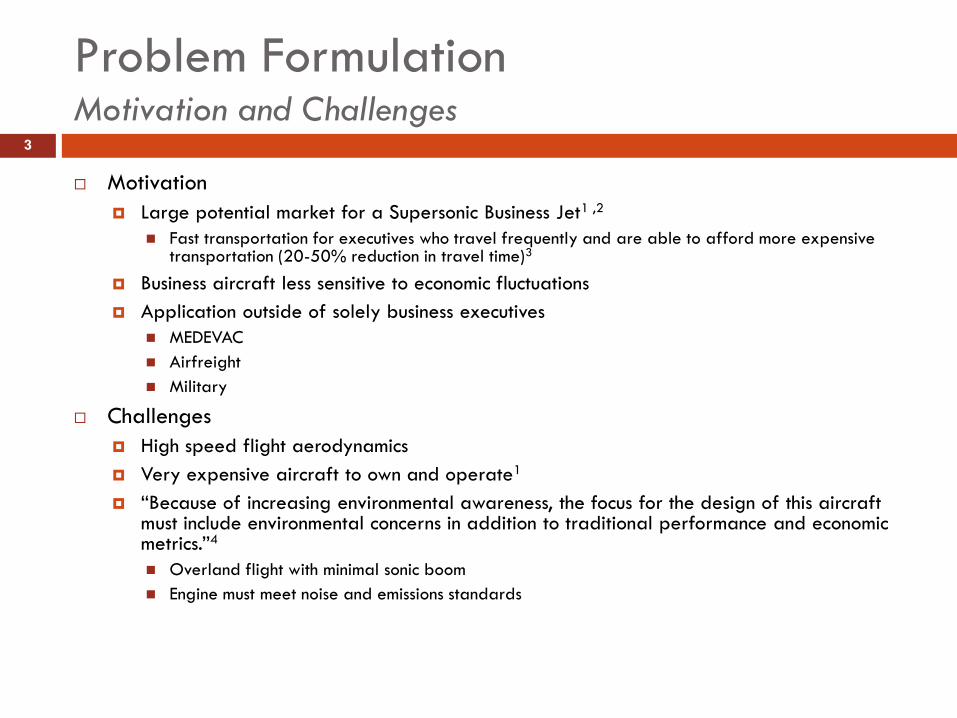
Motivation

Large potential market for a Supersonic Business Jet1 ,2

Fast transportation for executives who travel frequently and are able to afford more expensive transportation (20-50% reduction in travel time)3

Business aircraft less sensitive to economic fluctuations

Application outside of solely business executives

MEDEVAC

Airfreight

Military

Challenges

High speed flight aerodynamics

Very expensive aircraft to own and operate1

“Because of increasing environmental awareness, the focus for the design of this aircraft must include environmental concerns in addition to traditional performance and economic metrics.”4

Overland flight with minimal sonic boom

Engine must meet noise and emissions standards

Problem FormulationObjectives and Constraints

4

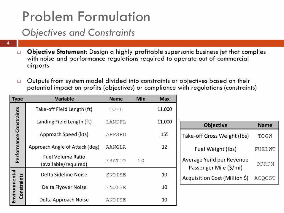
Objective Statement: Design a highly profitable supersonic business jet that complies with noise and performance regulations required to operate out of commercial airports

Outputs from system model divided into constraints or objectives based on their potential impact on profits (objectives) or compliance with regulations (constraints)

Objective Name

Take-off Gross Weight (lbs) TOGW

Fuel Weight (lbs) FUELWT

Average Yeild per Revenue

Passenger Mile ($/mi)DPRPM

Acquisition Cost (Million $) ACQCST

Type Variable Name Min Max

Take-off Field Length (ft) TOFL 11,000

Landing Field Length (ft) LANDFL 11,000

Approach Speed (kts) APPSPD 155

Approach Angle of Attack (deg) AANGLA 12

Fuel Volume Ratio

(available/required)FRATIO 1.0

Delta Sideline Noise SNOISE 10

Delta Flyover Noise FNOISE 10

Delta Approach Noise ANOISE 10Envi

ron

me

nta

l

Co

nst

rain

tsP

erf

orm

ance

Co

nst

rain

ts

Model and SimulationOverview

5

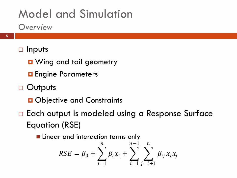
Inputs

Wing and tail geometry

Engine Parameters

Outputs

Objective and Constraints

Each output is modeled using a Response Surface

Equation (RSE)

Linear and interaction terms only

𝑅𝑆𝐸 = 𝛽0 + 𝛽𝑖𝑥𝑖

𝑛

𝑖=1

+ 𝛽𝑖𝑗 𝑥𝑖𝑥𝑗

𝑛

𝑗=𝑖+1

𝑛−1

𝑖=1

Model and SimulationOverview

6

Limitations/Features of RSE6

Accuracy only guaranteed in a small trust region

around sample points

Unable to predict multiple extrema

Assumes randomly distributed error (not usually the

case in computer experiments)

-0.05 -0.04 -0.03 -0.02 -0.01 0 0.01 0.02 0.03 0.04

XWING

XHT

XVT

X1LEKN

X2LETP

X3TETP

X4TEKN

X5TERT

Y1KINK

WGAREA

HTAREA

VTAREA

CFG

TIT

BPR

OPR

FANMN

FPR

ETR

SAR

TOTM

FNWTR

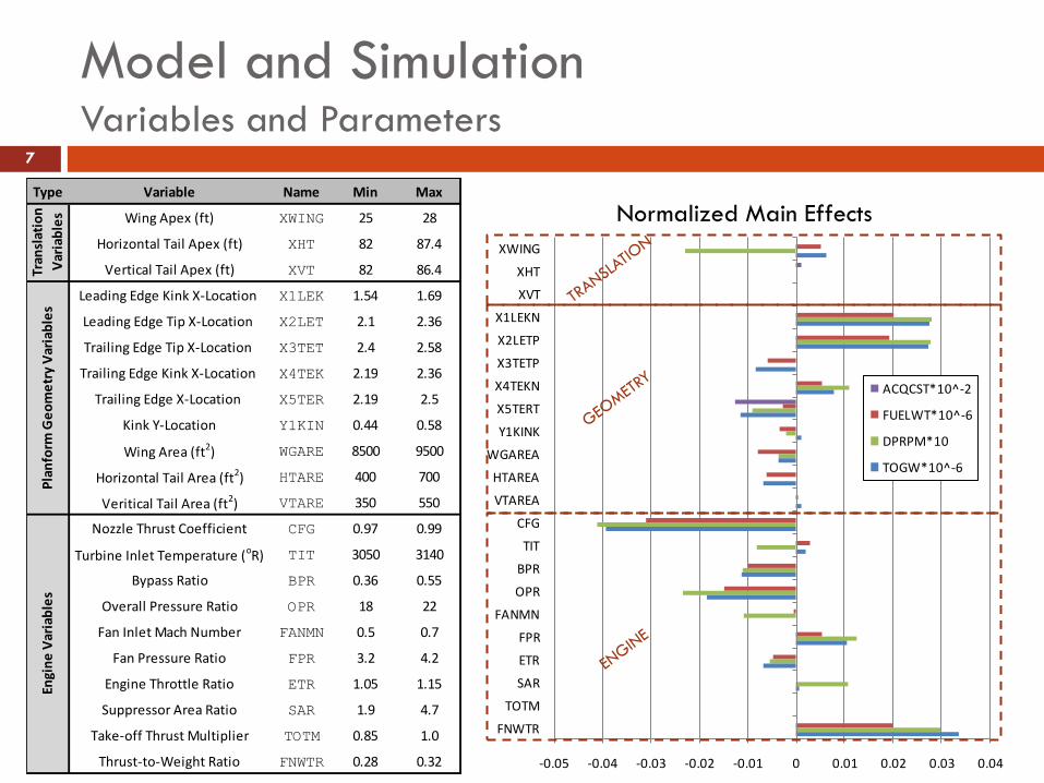
Variable & Parameter Influence

ACQCST*10^-2

FUELWT*10^-6

DPRPM*10

TOGW*10^-6

Model and SimulationVariables and Parameters

7

Type Variable Name Min Max

Wing Apex (ft) XWING 25 28

Horizontal Tail Apex (ft) XHT 82 87.4

Vertical Tail Apex (ft) XVT 82 86.4

Leading Edge Kink X-Location X1LEK 1.54 1.69

Leading Edge Tip X-Location X2LET 2.1 2.36

Trailing Edge Tip X-Location X3TET 2.4 2.58

Trailing Edge Kink X-Location X4TEK 2.19 2.36

Trailing Edge X-Location X5TER 2.19 2.5

Kink Y-Location Y1KIN 0.44 0.58

Wing Area (ft2) WGARE 8500 9500

Horizontal Tail Area (ft2) HTARE 400 700

Veritical Tail Area (ft2) VTARE 350 550

Nozzle Thrust Coefficient CFG 0.97 0.99

Turbine Inlet Temperature (oR) TIT 3050 3140

Bypass Ratio BPR 0.36 0.55

Overall Pressure Ratio OPR 18 22

Fan Inlet Mach Number FANMN 0.5 0.7

Fan Pressure Ratio FPR 3.2 4.2

Engine Throttle Ratio ETR 1.05 1.15

Suppressor Area Ratio SAR 1.9 4.7

Take-off Thrust Multiplier TOTM 0.85 1.0

Thrust-to-Weight Ratio FNWTR 0.28 0.32

Tran

slat

ion

Var

iab

les

Pla

nfo

rm G

eo

me

try

Var

iab

les

Engi

ne

Var

iab

les

Normalized Main Effects

Model and SimulationBenchmarking and Validation

8

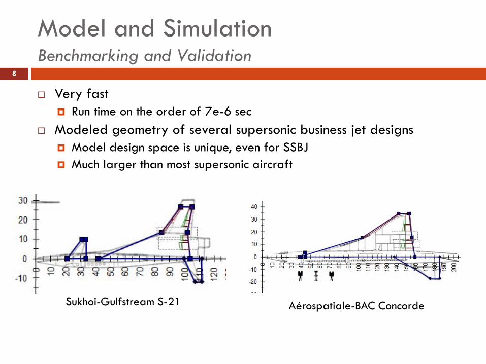
Very fast

Run time on the order of 7e-6 sec

Modeled geometry of several supersonic business jet designs

Model design space is unique, even for SSBJ

Much larger than most supersonic aircraft

Sukhoi-Gulfstream S-21 Aérospatiale-BAC Concorde

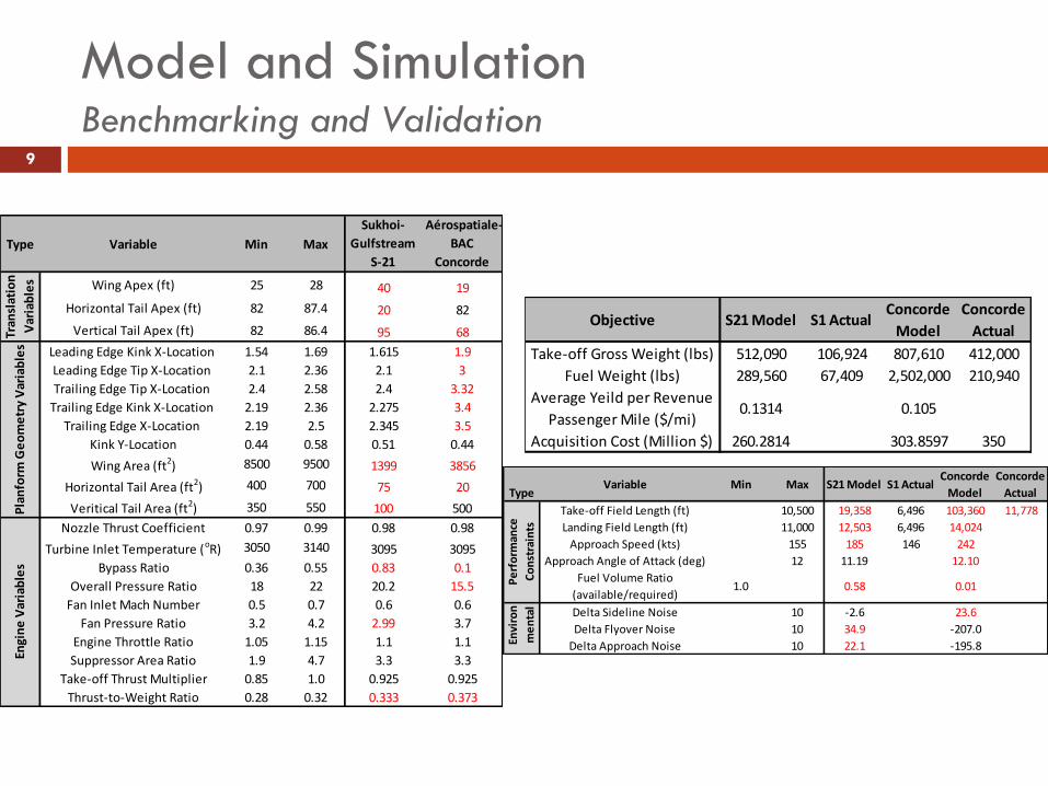
Model and SimulationBenchmarking and Validation

9

Type Variable Min Max

Sukhoi-

Gulfstream

S-21

Aérospatiale-

BAC

Concorde

Wing Apex (ft) 25 28 40 19

Horizontal Tail Apex (ft) 82 87.4 20 82

Vertical Tail Apex (ft) 82 86.4 95 68

Leading Edge Kink X-Location 1.54 1.69 1.615 1.9

Leading Edge Tip X-Location 2.1 2.36 2.1 3

Trailing Edge Tip X-Location 2.4 2.58 2.4 3.32

Trailing Edge Kink X-Location 2.19 2.36 2.275 3.4

Trailing Edge X-Location 2.19 2.5 2.345 3.5

Kink Y-Location 0.44 0.58 0.51 0.44

Wing Area (ft2) 8500 9500 1399 3856

Horizontal Tail Area (ft2) 400 700 75 20

Veritical Tail Area (ft2) 350 550 100 500

Nozzle Thrust Coefficient 0.97 0.99 0.98 0.98

Turbine Inlet Temperature (oR) 3050 3140 3095 3095

Bypass Ratio 0.36 0.55 0.83 0.1

Overall Pressure Ratio 18 22 20.2 15.5

Fan Inlet Mach Number 0.5 0.7 0.6 0.6

Fan Pressure Ratio 3.2 4.2 2.99 3.7

Engine Throttle Ratio 1.05 1.15 1.1 1.1

Suppressor Area Ratio 1.9 4.7 3.3 3.3

Take-off Thrust Multiplier 0.85 1.0 0.925 0.925

Thrust-to-Weight Ratio 0.28 0.32 0.333 0.373

Tran

slat

ion

Var

iab

les

Pla

nfo

rm G

eo

me

try

Var

iab

les

Engi

ne

Var

iab

les

TypeVariable Min Max S21 Model S1 Actual

Concorde

Model

Concorde

Actual

Take-off Field Length (ft) 10,500 19,358 6,496 103,360 11,778

Landing Field Length (ft) 11,000 12,503 6,496 14,024

Approach Speed (kts) 155 185 146 242

Approach Angle of Attack (deg) 12 11.19 12.10

Fuel Volume Ratio

(available/required)1.0 0.58 0.01

Delta Sideline Noise 10 -2.6 23.6

Delta Flyover Noise 10 34.9 -207.0

Delta Approach Noise 10 22.1 -195.8

Pe

rfo

rman

ce

Co

nst

rain

ts

Envi

ron

me

nta

l

Objective S21 Model S1 ActualConcorde

Model

Concorde

Actual

Take-off Gross Weight (lbs) 512,090 106,924 807,610 412,000

Fuel Weight (lbs) 289,560 67,409 2,502,000 210,940

Average Yeild per Revenue

Passenger Mile ($/mi)0.1314 0.105

Acquisition Cost (Million $) 260.2814 303.8597 350

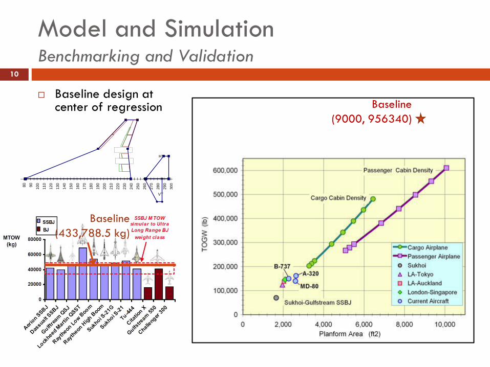
Model and SimulationBenchmarking and Validation

10

Baseline design at center of regression

-30

-20

-10

0

10

20

30

40

50

60

70

80

90

100

110

120

0

10

20

30

40

50

60

70

80

90

100

110

120

130

140

150

160

170

180

190

200

210

220

230

240

250

260

270

280

290

300

310

Y-l

oc (ft

)

X-loc (ft)

Overall Planform

VT

HT

Baseline

(9000, 956340)

Baseline

(433,788.5 kg)

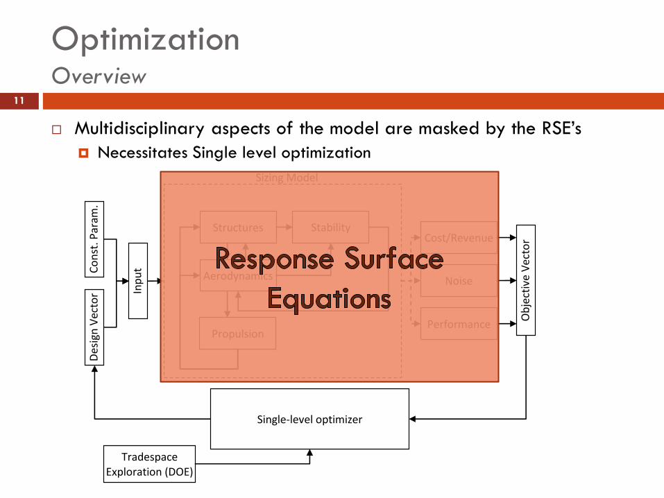
OptimizationOverview

11

Multidisciplinary aspects of the model are masked by the RSE’s

Necessitates Single level optimization

Stability

Propulsion

Structures

Aerodynamics

Ob

ject

ive

Vec

tor

Des

ign

Vec

tor In

pu

t Co

nst

. Par

am.

Single-level optimizer

Tradespace Exploration (DOE)

Performance

Noise

Cost/Revenue

Sizing Model

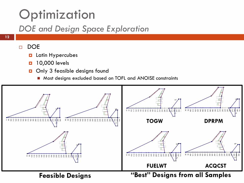
OptimizationDOE and Design Space Exploration

12

DOE

Latin Hypercubes

10,000 levels

Only 3 feasible designs found

Most designs excluded based on TOFL and ANOISE constraints

Feasible Designs

TOGW

FUELWT

DPRPM

ACQCST

“Best” Designs from all Samples

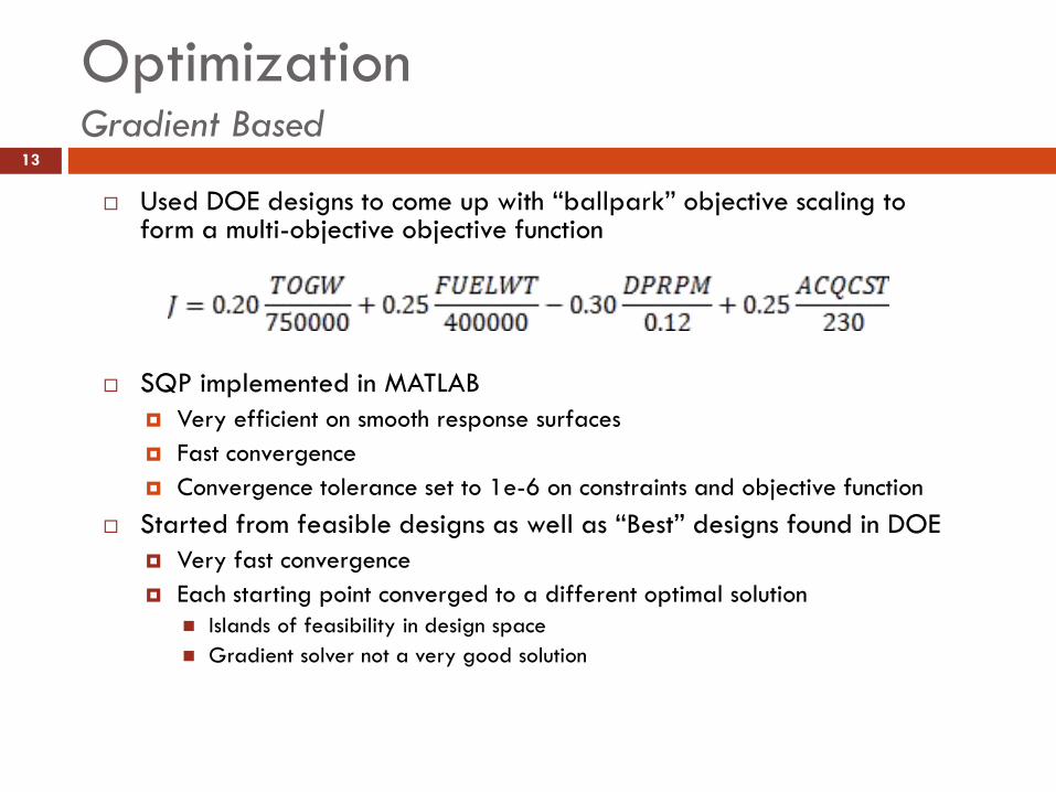
OptimizationGradient Based

Used DOE designs to come up with “ballpark” objective scaling to form a multi-objective objective function

SQP implemented in MATLAB

Very efficient on smooth response surfaces

Fast convergence

Convergence tolerance set to 1e-6 on constraints and objective function

Started from feasible designs as well as “Best” designs found in DOE

Very fast convergence

Each starting point converged to a different optimal solution

Islands of feasibility in design space

Gradient solver not a very good solution

13

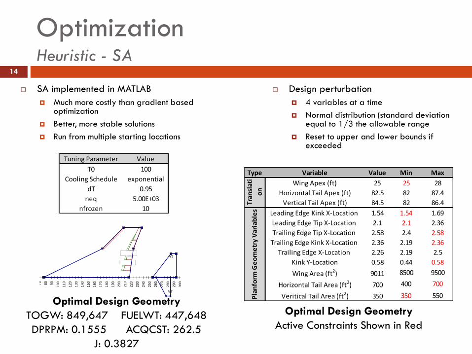
OptimizationHeuristic - SA

SA implemented in MATLAB

Much more costly than gradient based optimization

Better, more stable solutions

Run from multiple starting locations

Design perturbation

4 variables at a time

Normal distribution (standard deviation equal to 1/3 the allowable range

Reset to upper and lower bounds if exceeded

14

Optimal Design Geometry

TOGW: 849,647 FUELWT: 447,648

DPRPM: 0.1555 ACQCST: 262.5

J: 0.3827

Tuning Parameter Value

T0 100

Cooling Schedule exponential

dT 0.95

neq 5.00E+03

nfrozen 10

-30

-20

-10

0

10

20

30

40

50

60

70

80

90

100

110

120

0

10

20

30

40

50

60

70

80

90

100

110

120

130

140

150

160

170

180

190

200

210

220

230

240

250

260

270

280

290

300

310

Y-l

oc (ft

)

X-loc (ft)

Overall Planform

VT

HT

Type Variable Value Min Max

Wing Apex (ft) 25 25 28

Horizontal Tail Apex (ft) 82.5 82 87.4

Vertical Tail Apex (ft) 84.5 82 86.4

Leading Edge Kink X-Location 1.54 1.54 1.69

Leading Edge Tip X-Location 2.1 2.1 2.36

Trailing Edge Tip X-Location 2.58 2.4 2.58

Trailing Edge Kink X-Location 2.36 2.19 2.36

Trailing Edge X-Location 2.26 2.19 2.5

Kink Y-Location 0.58 0.44 0.58

Wing Area (ft2) 9011 8500 9500

Horizontal Tail Area (ft2) 700 400 700

Veritical Tail Area (ft2) 350 350 550

Tran

slat

i

on

P

lan

form

Ge

om

etr

y V

aria

ble

s

Optimal Design Geometry

Active Constraints Shown in Red

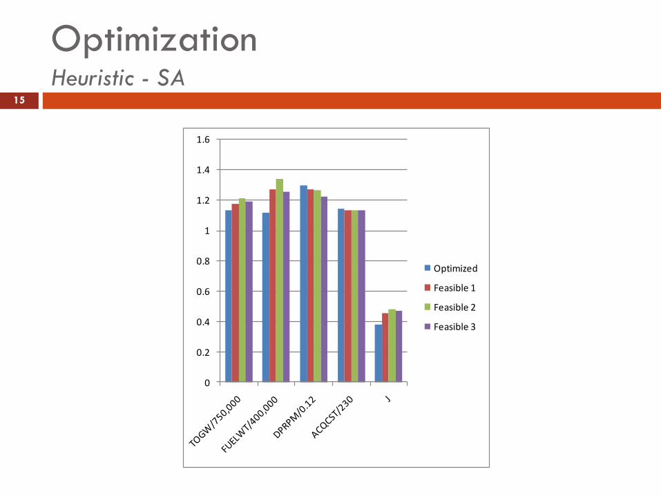
OptimizationHeuristic - SA

15

0

0.2

0.4

0.6

0.8

1

1.2

1.4

1.6

Optimized

Feasible 1

Feasible 2

Feasible 3

OptimizationMOO

16

Individual objective optimizations

Min TOGWTOGW: 825,974 FUELWT: 484,575

DPRPM: 0.1519 ACQCST: 267.0

Min FUELWTTOGW: 832,765 FUELWT: 438,856

DPRPM: 0.1583 ACQCST: 265.0

Max DPRPMTOGW: 932,407 FUELWT: 517,315

DPRPM: 0.1645 ACQCST: 264.1

Min ACQCSTTOGW: 826,734 FUELWT: 487,553

DPRPM: 0.1515 ACQCST: 255.7

-30

-20

-10

0

10

20

30

40

50

60

70

80

90

100

110

120

0

10

20

30

40

50

60

70

80

90

100

110

120

130

140

150

160

170

180

190

200

210

220

230

240

250

260

270

280

290

300

310

Y-l

oc (ft

)

X-loc (ft)

Overall Planform

VT

HT

-30

-20

-10

0

10

20

30

40

50

60

70

80

90

100

110

120

0

10

20

30

40

50

60

70

80

90

100

110

120

130

140

150

160

170

180

190

200

210

220

230

240

250

260

270

280

290

300

310

Y-l

oc (ft

)

X-loc (ft)

Overall Planform

VT

HT

-30

-20

-10

0

10

20

30

40

50

60

70

80

90

100

110

120

0

10

20

30

40

50

60

70

80

90

100

110

120

130

140

150

160

170

180

190

200

210

220

230

240

250

260

270

280

290

300

310

Y-l

oc (ft

)

X-loc (ft)

Overall Planform

VT

HT

-30

-20

-10

0

10

20

30

40

50

60

70

80

90

100

110

120

0

10

20

30

40

50

60

70

80

90

100

110

120

130

140

150

160

170

180

190

200

210

220

230

240

250

260

270

280

290

300

310

Y-l

oc (ft

)

X-loc (ft)

Overall Planform

VT

HT

-0.5 -0.4 -0.3 -0.2 -0.1 0 0.1 0.2 0.3 0.4 0.5

XWING

XHT

XVT

X1LEK

X2LET

X3TET

X4TEK

X5TER

Y1KIN

WGARE

HTARE

VTARE

CFG

TIT

BPR

OPR

FANMN

FPR

ETR

SAR

TOTM

FNWTR

TOGW

FUELWT

DPRPM

ACQCST

J

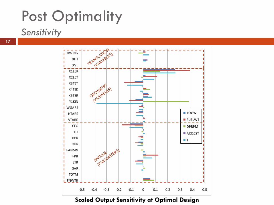
Post OptimalitySensitivity

17

Scaled Output Sensitivity at Optimal Design

Post OptimalityPareto Front and Trade-off Analysis

18

TOGW, FUELWT, and ACQCST are all mutually supportive

The trades occur with DPRPM

Pareto front: Using AWS approach

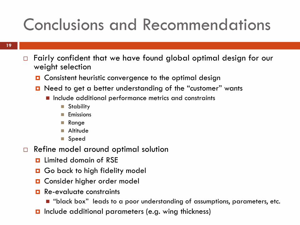
Conclusions and Recommendations19

Fairly confident that we have found global optimal design for our weight selection

Consistent heuristic convergence to the optimal design

Need to get a better understanding of the “customer” wants

Include additional performance metrics and constraints

Stability

Emissions

Range

Altitude

Speed

Refine model around optimal solution

Limited domain of RSE

Go back to high fidelity model

Consider higher order model

Re-evaluate constraints

“black box” leads to a poor understanding of assumptions, parameters, etc.

Include additional parameters (e.g. wing thickness)

References20

1. B. Chudoba & Al., “What Price Supersonic Speed ? – An Applied Market Research Case Study –Part 2”, AIAA paper, AIAA 2007-848, 45th AIAA Aerospace Sciences Meeting and Exhibit, Reno, 2007.

2. C. Trautvetter, “Aerion : A viable Market for SSBJ”, Aviation International News, Vol. 37 , No. 16, 2005.

3. Deremaux, Y., Nicolas, P., Négrier, J., Herbin, E., and Ravachol, M., “Environmental MDO and Uncertainty Hybrid Approach Applied to a Supersonic Business Jet,” AIAA-2008-5832, 2008.

4. Briceño, S.I., Buonanno, M.A., Fernández, I., and Mavris, D.N., “A Parametric Exploration of Supersonic Business Jet Concepts Utilizing Response Surfaces,” AIAA-2002-5828, 2002.

5. Federal Aviation Administration (FAA), “Federal Aviation Regulations (FAR)”, FAR91.817

6. Cox, S.E., Haftka, R.T., Baker, C.A., Grossman, B.G., Mason, W.H., and Watson, L.T., “A Comparison of Global Optimization Methods for the Design of a High-speed Civil Transport,” Journal of Global Optimization, Vol. 21, No. 4, Dec. 2001, pp. 415-432.

7. B. Chudoba & Al., “What Price Supersonic Speed ? – A Design Anatomy of Supersonic Transportation– Part 1”, AIAA paper, AIAA 2007-848, 45th AIAA Aerospace Sciences Meeting and Exhibit, Reno, 2007.

8. Chung, H.S., Alonso, J.J., “Comparison of Approximation Models with Merit Functions for Design Optimization,” AIAA 2000-4754, 200.

Backup21

Post OptimalityScaling

22

Objective function was scaled to be O(1)

Since the response surface does not have any

second order terms, the diagonal of the Hessian is 0

MIT OpenCourseWarehttp://ocw.mit.edu

ESD.77 / 16.888 Multidisciplinary System Design Optimization

Spring 2010

For information about citing these materials or our Terms of Use, visit: http://ocw.mit.edu/terms.