VALUING SCHOOL QUALITY USING

BOUNDARY DISCONTINUITIES

Stephen Gibbons*, Stephen Machin** and Olmo Silva***

November 2009

* Department of Geography and Environment and Centre for Economic Performance, London School of Economics

** Department of Economics, University College London and Centre for Economic Performance,

London School of Economics *** Department of Geography and Environment and Centre for Economic Performance, London School

of Economics Author for correspondence: Stephen Machin, Department of Economics, University College London, Gower Street, London, WC1E 6BT, UK. Email: s.machin@ucl.ac.uk

Acknowledgements: We would like to thank Amy Challen and Anushri Bansal for excellent research assistance, and Jaap Abbring, Victor Lavy, Erik Sørensen and participants at the Workshop on Residential Sprawl and Segregation 2007 (Dijon), the CEP Annual Meeting 2008 (Cambridge), the CEPR Economics of Education and Education Policy in Europe Conference 2008 (Amsterdam), and seminars at CPB - The Hague, Sussex University and Tinbergen Institute for comments and suggestions. We are responsible for any errors or omissions.

Abstract

A large body of international research shows that house prices respond to local school quality as measured

by average test scores. However, better test scores could signal better expected academic outputs or simply

reflect higher ability intakes, and existing studies rarely differentiate between these two channels. In our

research, we simultaneously estimate the response of prices to school value-added and school composition

to show more clearly what drives parental demand for schools. To achieve consistent estimates, we

improve the boundary discontinuity regression method by matching identical properties across admissions

authority boundaries; by allowing for a variety of boundary effects and spatial trends; by re-weighting our

data to only consider transactions that are closest to district boundaries; and by submitting our estimates a

number of potentially destructive falsification tests. Our results survive this battery of experiments and

show that a one-standard deviation change in either school average value-added or prior achievement

raises prices by around 3%.

Keywords: House prices; school quality; boundary discontinuities.

JEL Classifications: C21; I20, H75; R21.

- 1 -

1. Introduction

Good schooling is frequently upheld as decisive in life, but empirical evidence remains quite

ambiguous when it comes to answers about what makes a school ‘good’, and about what people

really value in education. Parents making school choices seem well aware of their preferences, and

go to great lengths to secure places for their children at their preferred schools. However, social

scientists have had mixed success in eliciting any general conclusions about these preferences.

Researchers in education have regularly used survey responses to learn about preferences for

schools (e.g. Coldron and Boulton, 1991; Flatley et al., 2001; and Schneider and Buckley, 2002).

The evidence from this field is that parents rank academic outcomes highly among the reasons for

choosing a school, but other factors play an important role, such as distance from home, school

composition, safety and well being. More recently, parents’ actual choices of schools and teachers

have been used as an alternative way to uncover preferences for school attributes (e.g. Hastings et

al., 2005; and Jacob and Lefgren, 2007).

Apart from these examples, the vast majority of research in the field has looked for evidence of

the value of schools in the capitalisation of their benefits into housing prices – i.e. the ‘hedonic’

valuation method. This wide-ranging international literature has shown that the demand for school

quality is at least partly revealed in housing prices whenever school places are assigned to

neighbouring homes. Gibbons and Machin (2008) and Black and Machin (2010) provide summaries

of recent evidence, suggesting a consensus estimate of around 3-4% house price premium for one

standard deviation increase in school average test scores. Bayer et al. (2007) offer a structural

modification based on discrete housing choices that provides a correction to the standard hedonic

framework when preferences are heterogeneous, and come to similar conclusions.

A limitation of this line of work is that – with only a few exceptions – it is confined to showing

that prices follow headline school performance measures based on school average test scores.

However, better school test scores could occur through improvements in school intake or through

- 2 -

faster pupil progress – potentially driven by teaching quality, school resources and peer effects. One

possibility is that parents pay for school output or value-added because it represents what they

expect their children to gain academically. A second possibility is that parents pay for good peers

and favourable school composition – which are school inputs – irrespective of the likely contribution

that these factors make to their own child's achievements1. While the first perspective is interesting

from a policy point of view because it puts a price on interventions that raise academic standards, the

second one is relevant because of its implications for school segregation (e.g. Epple and Romano,

2000). Clearly then it matters which of these drivers is important in determining house prices.

A handful of papers have taken steps to disentangle these two channels of influence. Brasington

and Haurin’s (2006) results appear to show that that school value-added and initial achievements

both have positive effects on prices, although this important point is lost in their conclusions. Kane

et al. (2005) also consider value-added and average test scores as alternative indicators of school

performance. However, they do not present specifications that include both indicators

simultaneously, and do not aim to provide persuasive evidence on the importance of value-added. In

contrast, Clapp et al. (2007) show that pupil ethnicity seems more important than test scores to home

buyers around Connecticut schools, although the authors do not have access to data on pupils’

academic progress. Other papers have looked at the importance of school expenditure relative to test

score outputs. For example, Downes and Zabel (2002) find that test scores are capitalised into local

house prices, whereas measures of school expenditures are not. Very recently, Cellini et al. (2008)

use referenda outcomes in California’s school finance system to suggest that house prices respond to

the level of capital expenditure per pupil and that this cannot be fully explained by changes in test

scores. Occasionally other school attributes have been considered. For example, Figlio and Lucas

(2004) find that state-assigned school ratings have a transient effect on prices, over and above test

1 See Kramarz et al. (2009) for a detailed discussion, together with empirical tests, of the relative importance of pupil, school and peer effects in determining test scores. Their findings suggest that a large part of the variation in test scores is explained by pupil attributes, followed by school quality differentials. On the other hand, peers’ characteristics matter less. This result is consistent with Gibbons and Telhaj (2008), Lavy et al. (2008) and most other studies on peer effects.

- 3 -

scores, suggesting that householders draw additional information about achievement from these

grades, or else value the ratings in their own right. Finally, Gibbons and Machin (2006) suggest that

popularity in itself raises prices, given that over-capacity schools command an additional premium

relative to under-capacity schools with equal performance.

Our paper moves this literature forward in a number of important ways. Our first contribution is

to clearly delineate the house price response to: (a) educational ‘value-added’, which we treat as the

school’s expected production output; and (b) intake composition, which we treat as a ‘consumption-

good’ aspect of school quality. To the best of our knowledge, our research is the first to use a

convincing identification strategy to show that parents value both school value-added and school

composition, even if the latter aspect is not a productive input in the educational production function.

Our second contribution is to improve and test the boundary discontinuity regression method,

which has become the favoured research approach in this field as a way to mitigate the effects of

endogeneity induced by unobserved neighbourhood characteristics. We make several innovative

contributions to this methodology, which can be summarised as follows: (a) We set out clearly the

assumptions involved in identifying school quality effects on prices from discontinuities at

admission zone boundaries; (b) We extend the method to a context in which school admission zones

are fuzzy, overlapping and only partially bounded; (c) We combine matching methods with the

regression-discontinuity design to allow for a fully non-parametric specification of the way housing

observables affect price differentials across boundaries; (d) We incorporate in our models a variety

of boundary fixed effects and spatial trends to account semi-parametrically for between-district

unobserved heterogeneity (e.g. in refuse collection and policing) and trends in amenities across

boundaries; (e) We make full and better use of the data by inverse-distance weighting our

regressions such that identification comes from variation at the admission zone boundaries where

neighbourhood heterogeneity is minimised, whereas previous work has restricted samples to within

fixed buffer-zones close to boundaries (e.g. 1/4 mile); (f) We perform a number of falsification

- 4 -

exercises and in particular a ‘killer’ falsification test which uses the quality of autonomous state

schools (church schools) that do not admit on the basis of residential location, but administer the

same standard tests as the mainstream schools that prioritise admission on place of residence.

A final advantage of our work is that we establish these findings using large scale

administrative data for the whole of England, and not just for one city (e.g. Boston or San Francisco)

as done by previous research. The size and coverage of our data makes the above strategies feasible.

Additionally, it allows us to disentangle the ‘price’ that parents are willing to pay for test score

progression as opposed to ‘consumption’ of better peers in a general and representative context.

To preview our results, our main finding is that a one-standard deviation change in school

average final test scores, brought about by either school value-added or prior achievement, raises

prices by around 3%. On the other hand, we show that there is no house price premium associated to

living close to high quality schools that do not admit based on residence. This test – alongside other

falsification exercises – demonstrates that our findings for schools that prioritise admissions on the

basis of school-home distance are causal and not spurious.2 In this respect, these exercises go much

further than any previous study in the field. Finally, various calculations show that the magnitude of

this house price response to school quality is plausible as a parental investment decision given the

expected return in terms of future earnings of their children.

The remainder of the paper has the following structure. Section 2 explains our methods. Section

3 discusses the context in which we apply these methods and the data setup. Section 4 presents our

results and discussion, focussing firstly on identification of the effects of school performance on

house prices, and then considering the role of value-added and school composition in this

relationship. Finally, Section 5 provides some concluding discussions.

2 Note that this is very different from the exercise of Fack and Grenet (2008), who concentrate on showing that house prices respond ‘less’ to the quality of local non-autonomous school if there are autonomous schools in the area. The authors cannot perform any falsification tests because their autonomous schools (unlike ours) are private schools and are not ‘ranked’ using comparable performance tables as state schools (once more, unlike our autonomous schools).

- 5 -

2. Empirical strategy

2.1. Methodological framework

Our empirical work uses a regression discontinuity design that builds on the geographical ‘boundary

discontinuity’ approach. This method was popularised for use in property value analysis by the work

of Black (1999), and has been employed several times since (e.g. Bogart and Cromwell, 2000;

Gibbons and Machin, 2003, 2006; Bayer and McMillan, 2005; Kane et al., 2005; Davidoff and

Leigh, 2007; Fack and Grenet, 2008; Bayer et al., 2007). Closely related thinking provides the

foundation of studies that investigate the effects of market access when there are changes in national

borders or their permeability. Examples include Redding and Sturm (2008), who look at changes that

occurred during German division and re-unification, and Hanson (2003) who focuses on the opening

of Mexican border as a result of the North American Free Trade Agreement. In a similar vein,

boundary discontinuities have been used to assess the effect of taxation on housing prices (Cushing,

1984), and on the location of manufacturing firms (Duranton et al., 2006; Holmes, 1998).

The standard ‘hedonic’ property value model is well known to economists (Sheppard, 1999).

This models property values (or, most commonly, log property values) as a linear combination of

observable property attributes and the ‘implicit prices’ of these attributes in the housing market.

These implicit prices can be estimated by standard least squares regression techniques. However, the

pervasive drawback with this approach is that researchers do not observe all salient property and

neighbourhood characteristics, leading to serious omitted variable issues. This problem is

particularly acute when neighbourhood amenity quality and local public good quality – like school

quality – depends on the distribution of characteristics in the local population. In such cases, any

unobserved attribute that raises local housing prices changes amenity quality through residential

sorting, because higher price houses are (on average) occupied by higher income households.

One way to mitigate this problem is to compare only close-neighbouring houses, because these

often tend to be quite structurally similar and self-evidently have near-identical neighbourhood

- 6 -

environments. Therefore, researchers can eliminate area effects in a house price model by taking

differences between houses that are in close proximity. However, this strategy is not useful for

obtaining implicit prices of neighbourhood attributes, unless there is a sharp discontinuity in the

supply of these attributes between close-neighbouring homes.

This last condition holds when school admissions are organised using contiguous pre-defined

admission zones: residents on one side of the boundary have access to a different school or set of

schools than do residents on the opposite side of the boundary. A researcher looking at the effect of

schools on house prices can therefore reduce the biases caused by unobserved neighbourhood

attributes by including attendance district boundary dummy variables in regression models (unless

the boundaries are particularly long), or by working with differenced data from a matched pair of

neighbouring houses on either side of the boundary. The empirical model underlying this approach is

set out below in a way that will help explain our empirical methods.

The price (p in logs) of a house sale, with characteristics ( )x c in a geographical location c , is:

( ) ( ) ( )p s c x c g cβ γ ε= + + + (1)

Where ( )s c represents the school ‘quality’ that home buyers expect to be able to access by

residence at c , prior to school admission, measured on the basis of school characteristics at periods

prior to the house sale. These characteristics include both school composition and effectiveness, and

in our empirical application we will try to estimate the effects of these different components

separately. As usual, ε represents unobserved housing attributes and errors that are assumed to be

independent of xandc . The function ( )g c represents unobserved influences on market prices that

are correlated across neighbouring spatial locations, such that the price varies deterministically with

geographical location, for example due to unobserved neighbourhood characteristics and amenities

(other than schooling). Location c can be specified in various ways, most flexibly in terms of a

vector of geographical or Cartesian coordinates. We discuss this in more detail below.

- 7 -

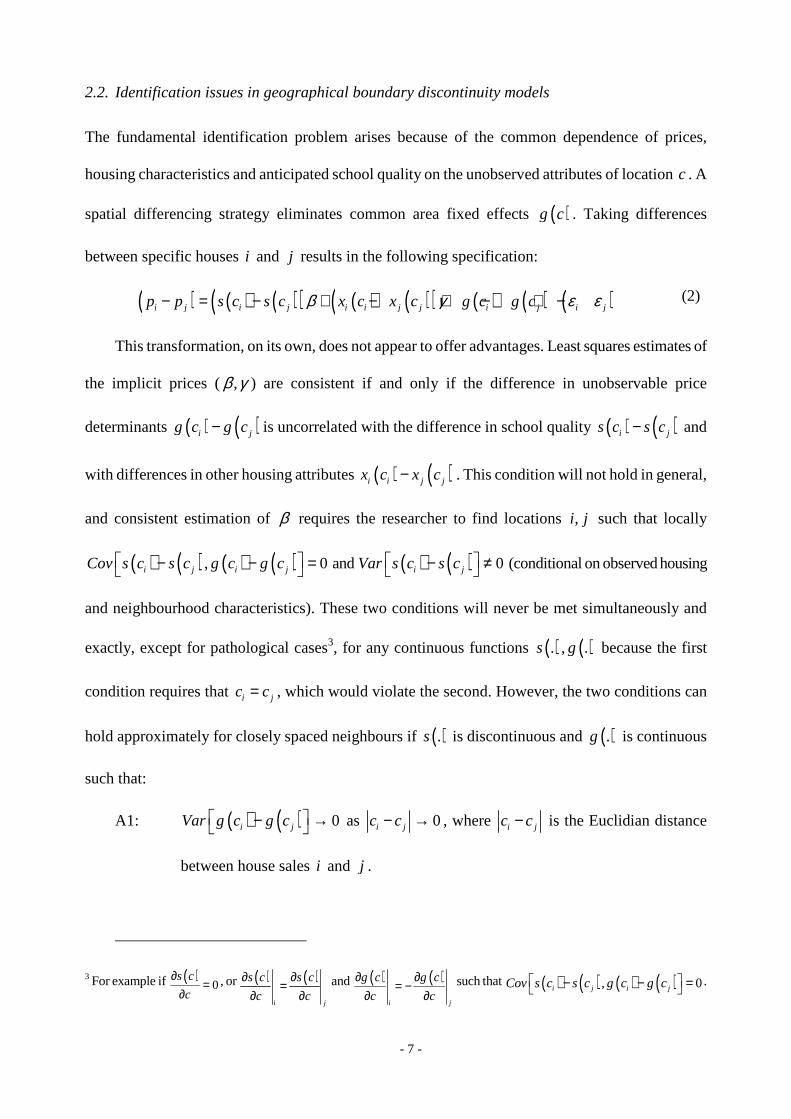
2.2. Identification issues in geographical boundary discontinuity models

The fundamental identification problem arises because of the common dependence of prices,

housing characteristics and anticipated school quality on the unobserved attributes of location c . A

spatial differencing strategy eliminates common area fixed effects ( )g c . Taking differences

between specific houses i and j results in the following specification:

( ) ( ) ( )( ) ( ) ( )( ) ( ) ( ) ( )i j i j i i j j i j i jp p s c s c x c x c g c g cβ γ ε ε− = − + − + − + − (2)

This transformation, on its own, does not appear to offer advantages. Least squares estimates of

the implicit prices ( ,β γ ) are consistent if and only if the difference in unobservable price

determinants ( ) ( )i jg c g c− is uncorrelated with the difference in school quality ( ) ( )i js c s c− and

with differences in other housing attributes ( ) ( )i i j jx c x c− . This condition will not hold in general,

and consistent estimation of β requires the researcher to find locations ,i j such that locally

( ) ( ) ( ) ( ), 0i j i jCov s c s c g c g c − − = and ( ) ( ) 0i jVar s c s c − ≠ (conditional on observed housing

and neighbourhood characteristics). These two conditions will never be met simultaneously and

exactly, except for pathological cases3, for any continuous functions ( ) ( ). , .s g because the first

condition requires that i jc c= , which would violate the second. However, the two conditions can

hold approximately for closely spaced neighbours if ( ).s is discontinuous and ( ).g is continuous

such that:

A1: ( ) ( ) 0i jVar g c g c − → as 0i jc c− → , where i jc c− is the Euclidian distance

between house sales i and j .

3 For example if ( )0

s c

c

∂=

∂, or ( ) ( )

i j

s c s c

c c

∂ ∂=

∂ ∂ and ( ) ( )

i j

g c g c

c c

∂ ∂= −

∂ ∂ such that ( ) ( ) ( ) ( ), 0i j i jCov s c s c g c g c − − =

.

- 8 -

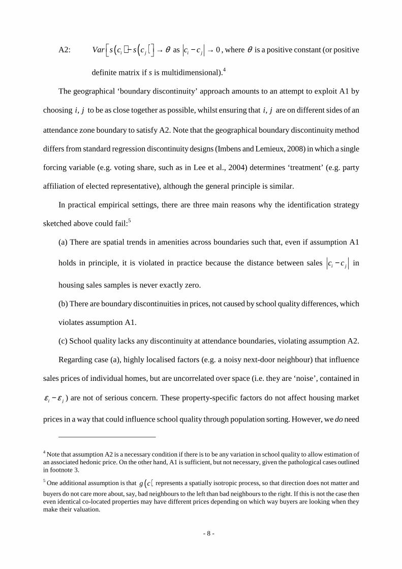
A2: ( ) ( )i jVar s c s c θ − → as 0i jc c− → , where θ is a positive constant (or positive

definite matrix if s is multidimensional).4

The geographical ‘boundary discontinuity’ approach amounts to an attempt to exploit A1 by

choosing ,i j to be as close together as possible, whilst ensuring that ,i j are on different sides of an

attendance zone boundary to satisfy A2. Note that the geographical boundary discontinuity method

differs from standard regression discontinuity designs (Imbens and Lemieux, 2008) in which a single

forcing variable (e.g. voting share, such as in Lee et al., 2004) determines ‘treatment’ (e.g. party

affiliation of elected representative), although the general principle is similar.

In practical empirical settings, there are three main reasons why the identification strategy

sketched above could fail:5

(a) There are spatial trends in amenities across boundaries such that, even if assumption A1

holds in principle, it is violated in practice because the distance between sales i jc c− in

housing sales samples is never exactly zero.

(b) There are boundary discontinuities in prices, not caused by school quality differences, which

violates assumption A1.

(c) School quality lacks any discontinuity at attendance boundaries, violating assumption A2.

Regarding case (a), highly localised factors (e.g. a noisy next-door neighbour) that influence

sales prices of individual homes, but are uncorrelated over space (i.e. they are ‘noise’, contained in

i jε ε− ) are not of serious concern. These property-specific factors do not affect housing market

prices in a way that could influence school quality through population sorting. However, we do need

4 Note that assumption A2 is a necessary condition if there is to be any variation in school quality to allow estimation of an associated hedonic price. On the other hand, A1 is sufficient, but not necessary, given the pathological cases outlined in footnote 3.

5 One additional assumption is that ( )g c represents a spatially isotropic process, so that direction does not matter and

buyers do not care more about, say, bad neighbours to the left than bad neighbours to the right. If this is not the case then even identical co-located properties may have different prices depending on which way buyers are looking when they make their valuation.

- 9 -

to be concerned about spatially correlated amenities that could lead house prices on one side of a

boundary to differ on average from house prices on the other side. This situation could arise if, for

example, one attendance zone contained a rail station and another did not (see Gibbons and Machin,

2005, for evidence of the amenity value of rail access). This would result in higher prices, richer

families and better schools in the ‘station zone’, and a spatial trend in house prices rising across the

boundary towards the station. Because of this trend, the price differential between houses on

different sides of the boundary grows with the distance between sales. Hence we could find a

correlation between house prices and school quality amongst closely spaced neighbours that is not

caused by the demand for school quality, but by residential sorting that is a consequence of demand

for rail access.

Even if there are no gradual cross-boundary price trends, there can be cases of type (b), where

prices change sharply from one side of the boundary to the other. First, administrative attendance

zone boundaries may coincide with distinct geographical features, e.g. major roads, which partition

communities. If these communities are different, the boundary may create a discontinuity in average

housing prices over short distances that is not school-related, violating the assumption that ( )g c is

continuous. Secondly, even without visible evidence of the boundary on the ground, houses on

different sides of a boundary could have different directional aspect or outlook. Consider, for

example, two long rows of houses on an east-west running boundary, one with sunny gardens facing

south and one with shady gardens facing north. If residents with children prefer sunny gardens, then

this aspect could be sufficient to induce a housing price differential and a consequent school quality

difference across the boundary. Thirdly, contiguous districts may have different tax rates or offer

different district-specific amenities, like refuse collection or policing, generating a sharp

discontinuity in prices that is not caused by schools.

Lastly, lack of discontinuity of type (c) occurs if attendance boundaries do not, in practice, act

as a barrier to pupils attending schools in districts neighbouring their homes. This could happen if

- 10 -

changes in school policy have removed the importance of traditional attendance zones. Note

however, that even if some pupils can cross these boundaries, condition A2 will still hold. In fact,

identification (in the sense of condition A2) requires only that there is a discrete jump in the

probability of attending schools on different sides of the boundary as one moves from a residence on

one side to a residence on the other, but this change in probability need not be from zero to one – i.e.

the discontinuity can be fuzzy (Imbens and Lemieux, 2007). This change in probabilities ensures that

there is a discrete jump in expected school quality (before admission) from one side to the other.

2.3. Proposed methods to address the identification problems

A few of these identification concerns have been partly addressed in the existing literature. However,

we take these problems into much deeper consideration and go a long way further than existing work

in establishing the credibility of the boundary discontinuity approach in our empirical context. With

this purpose, we extend the standard methodology and produce a series of powerful robustness and

‘falsification’ checks. These key extensions and tests are as follows (numbered method M1-M8 for

recognition in the Results section below):

M1. Visually assess and statistically test for the presence of discontinuities: Drawing on the

regression discontinuity design literature (and similar to Bayer et al., 2007, and Kane et al.,

2005), we provide some graphical evidence and statistical tests regarding such discontinuities in

area characteristics.

M2. Match property transactions with identical observable characteristics across administrative

boundaries. We pair up each house sale with the nearest transaction on the opposite side of an

administrative attendance district, where the transaction is of the same property type and occurs

in the same year (see also Gibbons and Machin, 2006, and to a lesser extent Fack and Grenet,

2008). This approach borrows from the literature on non-parametric discrete-cell matching, first

pioneered by Rubin (1973). In our set-up, this equates to allowing the price effects of matched

property characteristics to vary by boundary.

- 11 -

M3. Weight regressions to zero-distance housing transaction pairs. Earlier work (e.g. Black, 1999)

tested robustness to cross-boundary trends by selecting houses in increasingly narrow distance

bands along either side of the boundary, that is applying weights of 1 to transactions within a

specified boundary distance, and weights of 0 to those outside that distance. We generalise this

idea by weighting observations in inverse proportion to the distance between sales, such that

greater weight applies to observations that are close neighbours (on opposite sides of the

boundary). This is an important contribution of our approach, given that conditions A1 and A2

hold as the distance between paired transactions approaches zero. Re-weighting our analysis in

this way ensures that our identification predominantly comes from observations where the

identifying assumptions A1 and A2 are most likely to hold.

M4. Include boundary fixed effects in cross-boundary difference models. Our institutional context

(described below in Section 3) offers us multiple schools on each side of an attendance district

boundary, so school quality varies across boundaries and along a boundary within a given

attendance district. This data structure means we can control for boundary fixed effects (using

boundary dummy variables) in our cross-boundary differenced model, thus eliminating

between-boundary variation. This is crucial given assumption A1 and the problems with

boundary-specific discontinuities highlighted in Section 2.2 under case (b).

M5. Control for distance-to-boundary trends and polynomials. We follow the regression

discontinuity design literature by controlling for polynomial trends in ‘distance’ from the

discontinuity (e.g. DiNardo and Lee, 2004; Lee et al., 2004; and Clark, 2009). In our context,

this ‘distance’ is literally the geographical distance from attendance district boundaries. Like

other studies in this field, we impose some parametric structure, e.g. by specifying

( ) ( ) 2 3 2 311 12 13 21 22 23i j i i i j j jg c g c d d d d d dρ ρ ρ ρ ρ ρ− = + + + + + , where id is the distance from sale i to

the boundary, and jd is the distance from the matched sale j to the boundary. Note that we can

further control for different trends for each boundary by including boundary dummy × distance-

- 12 -

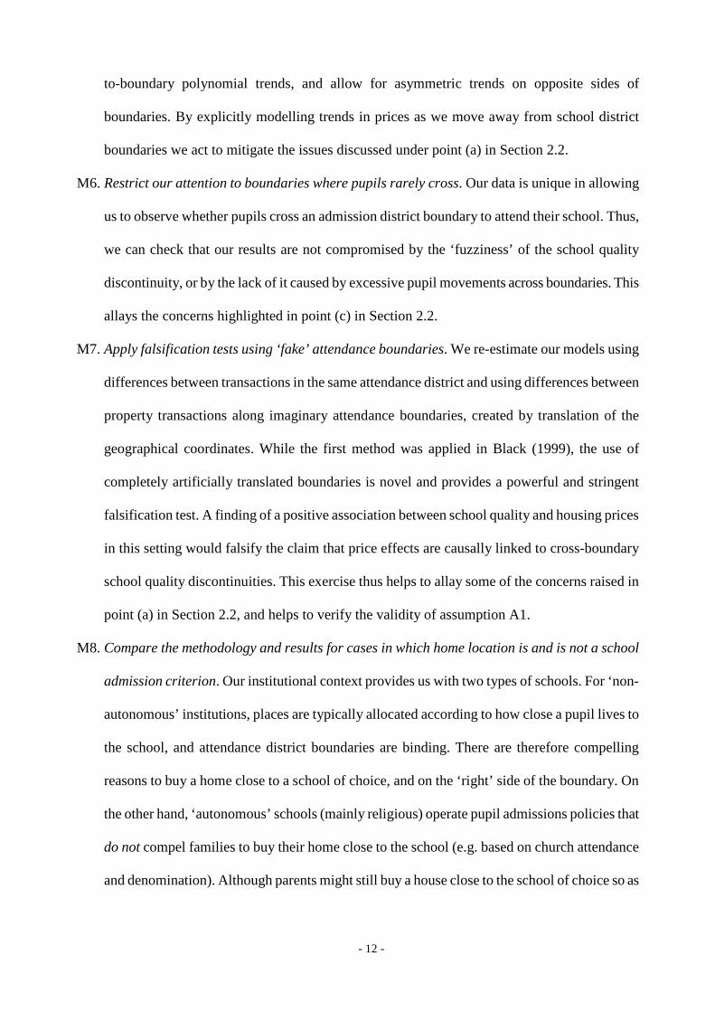
to-boundary polynomial trends, and allow for asymmetric trends on opposite sides of

boundaries. By explicitly modelling trends in prices as we move away from school district

boundaries we act to mitigate the issues discussed under point (a) in Section 2.2.

M6. Restrict our attention to boundaries where pupils rarely cross. Our data is unique in allowing

us to observe whether pupils cross an admission district boundary to attend their school. Thus,

we can check that our results are not compromised by the ‘fuzziness’ of the school quality

discontinuity, or by the lack of it caused by excessive pupil movements across boundaries. This

allays the concerns highlighted in point (c) in Section 2.2.

M7. Apply falsification tests using ‘fake’ attendance boundaries. We re-estimate our models using

differences between transactions in the same attendance district and using differences between

property transactions along imaginary attendance boundaries, created by translation of the

geographical coordinates. While the first method was applied in Black (1999), the use of

completely artificially translated boundaries is novel and provides a powerful and stringent

falsification test. A finding of a positive association between school quality and housing prices

in this setting would falsify the claim that price effects are causally linked to cross-boundary

school quality discontinuities. This exercise thus helps to allay some of the concerns raised in

point (a) in Section 2.2, and helps to verify the validity of assumption A1.

M8. Compare the methodology and results for cases in which home location is and is not a school

admission criterion. Our institutional context provides us with two types of schools. For ‘non-

autonomous’ institutions, places are typically allocated according to how close a pupil lives to

the school, and attendance district boundaries are binding. There are therefore compelling

reasons to buy a home close to a school of choice, and on the ‘right’ side of the boundary. On

the other hand, ‘autonomous’ schools (mainly religious) operate pupil admissions policies that

do not compel families to buy their home close to the school (e.g. based on church attendance

and denomination). Although parents might still buy a house close to the school of choice so as

- 13 -

to minimise travel costs, they do not need to do so to secure admission to their children. Thus,

we expect local house prices to respond to the quality of non-autonomous schools, but not to the

quality of ‘autonomous’ schools. This institutional feature provides us with a particularly

demanding ‘falsification’ test based on the comparison of the price response to the quality of

both types of schools as an additional check on the issues raised in points (a) and (b) in Section

2.2. We discuss these features of the school admission system in more detail in Section 3.2.

The robustness and falsification tests described above relate to identification of the causal effect

of school quality and other characteristics on house prices. We now turn to describe an additional set

of identification issues that arise when the research goal is to interpret the above estimates as

‘willingness to pay’ for school quality.

2.4. Identification in hedonic models when there is sorting on school quality

It is well known that empirical identification of marginal willingness to pay for any neighbourhood

amenity in a hedonic model is challenging when different households have different incomes and

different preferences for this amenity leading to residential sorting. Under these conditions, the

distribution of household characteristics near good quality schools will be different from the

distribution of characteristics of residents near poor quality schools, even if school quality is the only

factor determining house prices. This sorting has two consequences.

Firstly, linear regression estimates may not provide estimates of the mean valuation of school

quality, because the marginal willingness to pay (WTP) for school quality varies across the

distribution of household characteristics. Obviously, it is incorrect to simply model this

heterogeneity by interacting school quality with household characteristics (e.g. income), because if

WTP varies by characteristics, then these characteristics are endogenous in house price regression

models. The innovative paper by Bayer et al. (2007) builds on Berry et al. (1995), and focuses on

this particular identification problem. They describe a solution using a two-stage structural approach

that imposes a particular functional form on the residential choice and sorting process (coupled with

- 14 -

an instrumentation strategy). In terms of detail, the first stage in their estimator involves a

multinomial logit model on actual housing choices. Although technically impressive, this method

relies on strong and hard-to-test assumptions about the shape of the indirect utility function and on

the Independence of Irrelevant Alternatives (IIA) hypothesis invoked to estimate multinomial logit

models. It is thus difficult to generalise its applicability and understand the consequences of the

failure of any of the required assumptions. In our work, we do not wish to impose this much

structure, but present no novel solution to these issues. In the presence of heterogeneous preferences

and/or incomes and sorting across boundaries, our discontinuity design will provide a weighted

average of the marginal WTP of residents along the admissions zone boundary. This estimate may

be an upward or downward biased estimate of mean marginal WTP. However, in our defence, the

work by Bayer et al. (2007) shows that, both empirically and from a theoretical point of view, the

‘traditional’ hedonic models are effective at evaluating mean WTP in contexts (like ours) where the

amenity in question is supplied at various qualities in many different locations6.

For the same reasons, in this paper we also do not consider the issue of heterogeneity in the

responses of house prices to school quality depending on buyers’ or neighbourhood characteristics.

These are endogenous in house price regression models in the presence of sorting, and cannot be

simply added to empirical specifications in interaction with school quality.

The second consequence of sorting on school quality is that it makes it difficult to separate

marginal willingness to pay for school quality from the marginal willingness to pay for neighbours’

quality. In the presence of sorting, part (though clearly not all) of the association of between school

quality and house prices works through its effect on neighbour quality, so estimates cannot be easily

interpreted as WTP for school quality per se. Our robustness checks in this respect are limited to a

control variable strategy in which many of the neighbourhood demographic controls are potentially

6 The authors find a house price response of approximately 2.5% for a one standard deviation change in test scores in their ‘standard’ hedonic models, which rises to around 3% when accounting for the effects of sorting.

- 15 -

endogenous. Nevertheless, we will demonstrate that our estimates of the value of school quality are

steadfastly linked directly to school attributes, and in this control function context not to

neighbourhood quality.

3. Institutional context and data setup

Before presenting our results in the next Section of the paper, we offer a description of England’s

primary schooling system in more detail. We also discuss the data sources that we use to implement

our work and the empirical specifications that we consider.

3.1. National curriculum and assessment in England

Compulsory education in England is organised into five stages referred to as Key Stages. In the

primary phase, pupils enter school at age 4-5 in the Foundation Stage then move on to Key Stage 1

(ks1), spanning ages 5-6 and 6-7. At age 7-8 pupils move to Key Stage 2, sometimes – but not

usually – with a change of school.7 At the end of Key Stage 2 (ks2), when they are 10-11, children

leave the primary phase and go on to secondary school where they progress through Key Stage 3 and

4. At the end of each Key Stage, in May, pupils are assessed on the basis of standard national tests,

and progress through the phases is measured in terms of Key Stage Levels, ranging between W

(working towards Level 1) and Level 5+ in the primary phase. A point system can also be applied to

convert these levels into scores that represent about one term’s (10-12 weeks) progress.

Since 1996, in the autumn of each year, the results of the National Curriculum assessment at

Key Stage 2 are published as a guide to primary school performance. More recently, since 2003, a

value-added score has also been reported, based on the average pupil gain at each school between

age 7 and age 11 (relative to the national average). Schools and Local Education Authorities report

these performance figures in their admissions documents, and parents refer to these documents and

7 In few cases there are separate Infants and Junior schools (covering Key Stage 1 and 2 respectively) and a few LAs still operate a Middle School system (bridging the primary and secondary phases); we do not consider these schools here.

- 16 -

the performance tables, as well as using word-of-mouth recommendations, when choosing schools

(see, inter alia, Flatley et al., 2001 and Gibbons and Silva, 2009).

In our empirical work below, we use the ks1 to ks2 value-added score (va) as the main indicator

of schools’ production output, or effectiveness. On the other hand, we treat ks1 scores as a general

control for pupils’ prior academic achievements, i.e. mainly as a measure of school inputs in terms

of the educational advantages embodied in the composition of its pupil intake. These ks1 tests might,

at least in part, reflect the effectiveness of a school in children’s early years. However, they are not

publicly available and so cannot provide parents with a direct signal of school performance. Thus,

we treat ks1 scores as capturing information about school composition that parents can only learn

about from school visits, word of mouth, and using local knowledge.8 Our results in the following

sections seem to confirm that ks1 test scores are predominantly linked to students’ background

characteristics. Note also that if there were significant benefits to be had from schoolmates with

higher mean prior achievements (ks1) operating through peer effects, these would be capitalised in

house prices via school average value-added. Thus, conditional on school effectiveness (va), a

significant response of house prices to school composition is more likely to indicate parental demand

for peer quality as a consumption (non-productive) good. Finally, one further justification for

focusing on ks1 scores as an indicator of background (rather than income or free school meal

eligibility) is that the coefficient on value-added conditional on ks1 in our regressions can be easily

interpreted in terms of pupil progress or final achievement.

3.2. School types and admissions

All state primary schools in England are funded largely by central government, through Local

Authorities (LAs, formerly Local Education Authorities) that are responsible for schools in their

8 Note however that performance tables contain information on the fraction of students with special education needs (SEN), with varying degrees of severity. SEN status is partly based on poor performance in early tests and assessments. Thus parents can gather some indirect information about the intake quality of a school using performance tables.

- 17 -

geographical domain. These schools fall into a number of different categories, and differ in terms of

the way they are governed and who controls pupil admissions. 9 Most primary schools (roughly two-

thirds) are termed ‘Community’ schools and are closely controlled by the LA. Other types of school,

instead, are usually linked to a Faith or other charitable organisation, and more autonomously run.

The key difference relevant to this paper is between schools that administer their own admissions

and make their own choices on whom to admit – which we term autonomous schools – and non-

autonomous schools such as Community schools to which pupils are assigned by the Local

Authority. Gibbons et al. (2008) provide more details on the overall differences between these two

groups of schools.

Regarding pupil admissions, overall, all LAs and schools must organise their arrangements in

accordance with the current (now statutory) School Admissions Code. The guiding principle is that

parental choice should be the first consideration when ranking applications to a primary school.

However, if the number of applicants exceeds the number of available places, almost any criterion,

which is not discriminatory, does not involve selection by ability and can be clearly assessed by

parents, can be used to prioritise applicants. These criteria vary in detail, and change over time, but

preference in non-autonomous schools is usually given first to children with special educational

needs, next to children with siblings in the school and, crucially, to those children who live closest.

For Faith and other autonomous schools, regular attendance at designated churches and other

expressions of religious commitment are of foremost importance. Place of residence, in contrast,

almost never features as a criterion. Even then, if place of residence is important for admission, it

relates to Diocese boundaries, which do not follow administrative and school admission boundaries.

Consequently, there is little reason for parents to pay for homes close to good autonomous schools,

other than to reduce travel costs.

9 LAs are responsible for the strategic management of state education services, including planning the supply of school places, intervening where a school is failing and allocating central funding to schools. In addition there is a small private, fee-paying sector, which we do not consider here. Private schools educate around 6-7% of pupils in England as a whole.

- 18 -

There is however one additional crucial feature of the admission system that applies to non-

autonomous, but not to autonomous schools, and that we exploit in our empirical work. Pupils rarely

attend non-autonomous schools outside of their LA of residence. Families are allowed to apply to

non-autonomous schools in other LAs, but up until recently (covering the period we consider in our

empirical work) parents had to make separate applications to different LAs. More importantly, LAs

do not have a statutory requirement to find a school for pupils from other school districts: the law

only requires that they provide enough schools for pupils in “their area”.10 As a result, banking on

admission to a popular non-autonomous school in another LA is a high-risk strategy and LA

boundaries act as admissions district boundaries over the period we study. This provides a source of

discontinuity in the non-autonomous school ‘quality’ that residents can access on different sides of

LA boundaries. In contrast, these barriers are much less relevant for admission to Faith schools and

other autonomous schools that manage their own admissions. In Section 4.2 below, we will provide

clear and compelling evidence that LA boundaries significantly affect non-autonomous school

attendance patterns, and that there is a discrete jump in the probability of attending schools in a

given admission district as one moves from a residence on one side to a residence on the other side

of a boundary.

3.3. Source data

In our analysis we combine information obtained from three different data sources. Our source of

price information is the “Price-paid” dataset from the UK Land Registry for the years 2000-2006.

This is an administrative dataset that records the address, sales price and basic characteristics

(property type, new or old build, freehold or leasehold) of all domestic properties sold in the UK.

Each property is located by its address postcode, typically 15 neighbouring addresses, and each

10 More precisely, the Education Act 1996 section 14 reads: “(1) A Local Education Authority shall secure that sufficient schools for providing (a) Primary education, and (b) education that is Secondary education (…) for their area. (2) The schools available for an area shall not be regarded as sufficient (…) unless they are sufficient in number, character and equipment to provide for all pupils the opportunity of appropriate education”.

- 19 -

postcode can be assigned to a 1 metre coordinate on the British National Grid system using the

National Statistics Postcode Directory.

Information on school quality and characteristics comes from the UK’s Department for

Children, Schools and Families (DCSF ). The DCSF collects a variety of census data on state-school

pupils centrally, because the pupil assessment system is used to publish school performance tables

and because information on pupil numbers and characteristics is necessary for administrative

purposes – in particular to determine funding. A National Pupil Database exists since 1996 holding

information on each pupil’s assessment record in the Key Stage Assessments throughout their school

career. Since 2002, a Pupil Level Annual Census (PLASC) records information on pupil’s school,

gender, age, ethnicity, language skills, any special educational needs or disabilities, entitlement to

free school meals and various other pieces of information including postcode of residence. PLASC is

integrated with the pupil’s assessment record in the National Pupil Database (NPD), giving a large

and detailed dataset on pupils along with their test histories. Additional institutional characteristics

and expenditure information on schools is obtained from “Edubase” data, from the Annual School

Census and from the Consistent Financial Reporting series that can be obtained from the DCSF.

Finally, neighbourhood characteristics from the 2001 GB Census at Output Area level are

linked to the Price-paid housing transactions data by their address postcode. We also compute

various geographical attributes such as distances to LA boundaries and distances between properties

using a Geographical Information System.

Linking the schools data to housing sales is more complex, since there is no predefined mapping

between a house sale, i.e. its postcode, and the set of schools that are accessible from that location.

We infer this mapping from actual home-school travel-patterns using a computationally intensive,

but intuitively simple procedure as described in the next section.

- 20 -

3.4. Linking schools to housing transactions and matching across boundaries

One of the innovations in this work is the accurate assignment of school quality to house location in

institutional settings such as ours, where there is no one-to-one mapping between where a child lives

and the school he or she attends. The procedure entails imputation of the set of schools accessible

from each postcode in our Land Registry housing transactions database using the attendance patterns

of pupils that are recorded in the National Pupil Database. This approach is much more sophisticated

than the common approach of simply assigning a house to the nearest school or set of schools, and is

essential when we want to exploit boundary discontinuities. Defining catchment areas from

‘revealed preferences’ in this way implicitly accounts for features of school choice and attendance

patterns that would be obscured by simpler assignment rules.

In our revealed preference procedure, we start by estimating the approximate shape of the

catchment area for each school using the residential addresses (postcode) of pupils in the year when

they start at the school. This shape is delineated by the 75th percentile of the home-to-school distance

in each of 10 sectors radiating from each school location (starting West and moving anticlockwise).

Each of the 10 sectors is drawn to capture 10% of the school’s intake. This procedure relaxes

constraints on the shape of catchment areas, allowing for geographically asymmetric patterns of

attendance with sufficient flexibility to apply our boundary discontinuity design. The reason we

truncate the catchment areas at the 75th percentile home-school distance in each direction is to

remove outliers that could artificially inflate the size of the imputed school catchment areas.

Discarding these outliers reduces the likelihood that we erroneously draw catchment areas across LA

boundaries, and ensures that we focus on areas in which there is a high chance of admission – a

consideration which is paramount to home buyers seeking to get their children into a particular

school (and thus to our research). Note that we experimented with various distance thresholds, as

well as with overlapping fixed interval radial sectors and alternative starting points and orientations,

with little effect on the results.

- 21 -

Before moving on, let us emphasise why this shaping procedure is necessary by considering

some alternatives. Suppose we simply assigned the quality of the nearest school to each housing

transaction, or arbitrarily drew a circular catchment area around each school. To implement a

boundary discontinuity strategy, we would need to artificially impose the constraint that a student in

a house on one side of an administrative attendance district boundary (i.e. the LA boundary) can not

attend their nearest school if it lies on the other side. Without this restriction, the set of schools

available close to an admissions zone boundary, but on opposite sides of it, would be nearly identical

to each other. Hence, there would be no source of variation in school quality for identification in the

boundary discontinuity model (violating Assumption A2). On the other hand, we would not want to

impose this constraint if the discontinuity did not actually exist. Our imputation procedure does not

force any such truncation of the catchment area at the boundary unless it is supported by the spatial

distribution of pupil homes in relation the schools they attend. Stated differently, we allow the

catchment areas of schools close to the LA boundaries to be truncated and shrunk in the direction of

the boundaries – as well as in any other areas and trajectories – only when the data reveal that this is

the ‘right’ pattern.

After creating each school-specific catchment area definition, we calculate the distance and

direction from each school to each housing transaction in our Land Registry housing transactions

database (up to a maximum distance of 10km). It is then straightforward (though time consuming) to

link each house to multiple schools by deducing which housing transactions lie within which school

catchment areas. Following that, we calculate variables summarising the set of schools that are

accessible from a given housing transaction postcode in a given year, by averaging the

characteristics of the schools to which a house is linked (note that we average using higher weights

on the closest schools to each house, although results are similar when using un-weighted means). In

carrying out this aggregation we maintain the distinction between autonomous and non-autonomous

- 22 -

schools. So, for example, a housing transaction is assigned the mean value-added of local non-

autonomous schools and the mean value-added of autonomous schools as separate variables.

We also take care to correctly organise the timing of events in our data. The pupil census in

England occurs in January, pupils take their ks1 and ks2 assessments in May, and the results are

published towards the end of the calendar year. We therefore link prices of houses sold in calendar

year t (January to December) to the test results and census figures published at the end of year t-1 (in

October to November).

The procedure described above yields a large dataset of over 1.6 million housing sales for 2003,

2004, 2005 and 2006 joined to data on the average characteristics of the set of schools that can be

accessed from the postcode of each sale. To set up the spatially differenced cross-boundary model in

Equation (2) we reduce our sample to the set of sales occurring within 2500m of a LA (attendance

district) boundary. We then find, for each transaction, the nearest sale in the same year of the same

property type, occurring in an adjacent LA, within the median inter-property distance across that

specific boundary (method M1 in Section 2.3). This means that a given housing sale can provide a

‘match’ for multiple housing sales. Note that property type here is defined by detached, semi-

detached, terraced or flats, and by ownership type, i.e. leasehold or freehold. Further, the restriction

on matching within median distance along a boundary ensures that we do not create any matched

pairs that are excessively far apart, given the density of houses in the local area. For reasons

explained in Section 2.3, we also set up a set of matched sales across ‘fake’ LA boundaries and a set

of matched sales within LAs (method M7). To produce the first sample, we simply translate the

geographical coordinates of the housing transactions data by 10km North and 10km East, and repeat

the matching exercise. For the second, we repeat the matching exercise but impose the constraint

that the matched sale is within the same LA and at least 20m away to achieve better comparability

with the cross-LA samples.

- 23 -

3.5. Empirical specification

Applying the data described above to the models of Equations (1) and (2) yields empirical

specifications of the form:

( )1 2 1hi i i i hi i hip va ks z x g cβ β λ γ ε′ ′= + + + + + (3)

( )1 2 1hi i i i hi i hip va ks z x g cβ β λ γ ε′ ′∆ = ∆ + ∆ + ∆ + ∆ + ∆ + ∆

In equation (3), hip is the (log) price of the house sale h in location i ; iva is the expected value-

added and 1iks is the mean age-7 test score, for schools that can be accessed from location i

(measured at periods prior to the house transaction); the vector iz contains other observable school

and neighbourhood characteristics; vector hx contains observable attributes of house sale h ; and the

function ( )ig c represents unobserved neighbourhood characteristics and amenities (other than

schooling) that affect market prices. We parameterise ( )ig c using boundary dummy variables,

distance to school, distance between matched transactions and various distance-to-boundary

polynomials. As usual, iε represents unobserved housing attributes and errors that are independent

of all other factors (i.e. ‘noise’). The notation ∆ means a difference between matched, closest

transactions on either side of the LA boundary.

Although we have house sales and school attributes in multiple periods, we have suppressed the

t-subscripts for simplicity. Variation over time in the cross-boundary differences in school quality

contributes to identification, but we do not exploit the time dimension alone in our estimation

strategy. Three reasons for this decision are: (a) test scores assigned to house postcodes are highly

correlated from one period to the next so that the within-place, between-period variance in school

quality is low; (b) we have only 3 full years (2003, 2004 and 2005) and one quarter (quarter 1 of

2006) of housing transactions linked schools data; and (c) response of prices to changes is likely to

display inertia and be sluggish. These factors mean we cannot use changes over time alone as a basis

- 24 -

for identification. In the next section we present results from regression estimates of the models in

(3) obtained by pooling all available time periods.

4. Results

4.1. Descriptive statistics

Table 1 presents some key descriptive statistics. The first two columns summarise the full data set of

housing transactions and associated school characteristics from 2003-2006. The second two columns

present comparable statistics for our boundary sub-sample of sales, described in the Data section

above. The average price of sales in the transactions data set is £182,730. In the boundary sub-

sample the mean is about £13,000, or 7% higher. This is because administrative boundaries are more

prevalent in and around towns and cities and hence we pick up more urban transactions in the

boundary sub-sample. In addition, there is a greater chance of finding matched pairs of sales across

sections of the boundaries in urban areas, where housing is denser. It is easy to visualise this in

Figure 1, which plots the locations of transactions in the boundary sub-sample for two arbitrarily

chosen geographical area: the Midlands, North West and South Yorkshire (Panel A); and London

and the South East (Panel B). The figure illustrates a general spread of sales throughout England’s

cities and towns, but in a way that is governed by the administrative boundary structure.

In terms of school test scores, value-added is higher in the boundary sub-sample and ks1scores

are lower, but the differences are relatively small. Houses in this sub-sample have slightly fewer

accessible schools (where accessibility is imputed from travel patterns described in the Data section

above). This difference is in accordance with our claim that LA boundaries restrict the choice set for

houses located close to the boundary (see the discussion above and Gibbons et al., 2008). Schools

also tend to be closer to home in the boundary sub-sample, again reflecting the relatively urban

nature of the sample.

- 25 -

For the boundary group, we also present some statistics on the distance to the closest boundary

and the distance between property pairs that are matched across boundaries. The raw mean distance

to the boundary is nearly 500 metres, and the raw average distance between matched properties is

just under 725 metres. These figures look high in comparison with previous studies that focus on city

neighbourhoods only, but are not so large in the light of the general geographical spread illustrated

in Figure 1. In our regressions, we apply inverse inter-sale distance weights, so the inverse distance

weighted (IDW) means provide a better representation of the effective boundary difference relevant

to our regressions. The effective mean distance to the boundary in the weighted sample is only

133m, and the weighted inter-sale distance only 206m.

4.2. Evaluating the boundary discontinuities

As discussed at length in Section 2.2, a pre-requisite of our method is that a discontinuity exists in

school quality at LA boundaries (or in the school quality households expect to be able to access; see

Assumption A2). As a preliminary step, we show that cross-district school attendance is much less

prevalent than within-district attendance, even close to district boundaries. The relevant figures are

presented in Table 2 and refer to proportions in the postcode. In the full dataset, only 3.3% of pupils

attend schools other than in their home LAs, though this is not surprising given that, on average,

schools in other LAs will be further away. In the boundary sub-sample the proportion rises to 6.2%,

while the IDW mean proportion crossing from each residential postcode in our sales data (given that

the postcode has any children of primary school entry age) is 25%. Since this figure corresponds to

addresses only 133m from the boundary (Table 1), we would expect nearly 50% chances of

attending a school on either side of the boundary if this did not impose a ‘barrier’ and was

unimportant for admission. Moreover, these means are from distributions that are highly right-

skewed and the median proportion of pupils attending a school in a district different is zero. Clearly,

then, LA boundaries create a strong impediment to school choice. This is fully consistent with the

- 26 -

results using boundary discontinuities to identify the causal impact of school choice and competition

on pupil achievement in Gibbons et al. (2008) (see also Card et al., 2008).

More explicit tests for discontinuities in school quality and other area characteristics at the LA

boundary are provided in Figure 2 and Figure 3 (using method M2 of Section 2.3). In all these

figures, the x-axis reports the distance from a property transaction to the LA boundary. The right

hand side of the diagram (distance > 0) corresponds to sales which have access to greater school

value-added than their match across the boundary, i.e. ( ) ( ) 0i js c s c− > in Equation (2). On the other

hand, the left side of the diagram (distance < 0) corresponds to cases where access is to schools with

value-added below that on the other side of the boundary. The plots are obtained as predictions from

a regression of the cross-boundary difference in the relevant variable, on a positive side and negative

side constant term, and 18 distance-decile dummies, up to 800m from the boundary on each side.

The dependent variables are standardised by the standard deviation of the cross-boundary difference

within 800m. The dotted lines show 95% confidence intervals. The plots are restricted to 400m on

each side for clarity, and shown alongside a test for whether the differences on both sides at the

boundary are equal (i.e. an F-test of the hypothesis that the absolute values of the positive and

negative constants in the regressions are equal to one another). Note that the reason why these

graphs are not necessarily symmetric is that a sale i on the ‘good’ side of the boundary may be

matched with its closest sale j on the ‘bad’ side of the boundary, but sale j may in turn be matched to

another sale k on the ‘good’ side of the (same or a different) boundary if j is closer to k than i. Note

also that it is simply an artefact of the construction of the graphs that the lines do not reach the

boundary, because the first point on the horizontal axis is the mean distance of the first decile of

housing transactions, ranked by distance to the boundary. Finally, the standard errors are clustered

on location jc to allow for repeated matches of the same sale j to multiple sales i, and for a degree of

arbitrary spatial correlation in the error term.

- 27 -

The top left panel of Figure 2 shows a large and sharp discontinuity in value-added scores at LA

boundaries for non-autonomous schools, making it clear that we have substantial variation in our

main school performance measure across boundaries (Assumption A2). The overall scale of the

difference within the 400 metres of the boundary is unsurprising given this is the variable on which

the right and left halves of the plot are defined. However, the most important point here is that

almost half of the 2-standard deviation spread occurs within the first 100m, from where our

identification will predominantly come. The top right panel shows that a discontinuity in house sale

prices exists too: although visually this looks small, the difference across the boundary is highly

significant, and the price on the ‘good’ boundary side is higher than the price on the ‘bad’ boundary

side at every corresponding distance. Rough visual comparison of the top left and right panels

suggests that a 0.8 standard deviation change in school average value-added is associated with a 0.05

standard deviation change in house prices at the boundary. As we move away from the boundary,

focussing on more widely spaced properties, we see that prices tend not to follow school average

value-added. This occurs because many other amenities drive these spatial price trends, illustrating

the importance of weighting our regression estimates to close-neighbour observations, and

controlling for distance-to-boundary trends (methods M3 and M5 in Section 2.3).

In the lower two panels of Figure 2, we look at the corresponding cross-boundary discontinuity

picture for autonomous school quality. In these graphs, the right hand side corresponds to places

with relatively high autonomous school quality (and vice versa for the left hand side). Again, there is

by definition a strong rise in school quality across the boundary. However, there is no sizable

discontinuity in house prices at the boundary in this institutional context, where admission to school

is not linked to where pupils live. In fact the p-value of the F-test (= 0.76) shows that one cannot

reject the null hypothesis of no cross-boundary difference in house prices.

In Figure 3 we present similar pictures for a range of neighbourhood-related characteristics,

with left and right sides split by low and high non-autonomous school average value-added. These

- 28 -

plots serve to show to what extent cross-boundary neighbourhood differences are correlated with

cross-boundary non-autonomous school value-added differences. It is evident that there are no

discontinuities in terms of a wide range of neighbourhood characteristics (obtained from the 2001

GB census and the Land Registry data), including the share of local dwellings sold per year, the

dwelling size and residents’ characteristics. One exception is the proportion high-qualified residents

(degrees and equivalent), in which there is a statistically significant break. The fact that more highly

educated residents live on the side of the boundary with good schools is evidence for some degree

sorting of those with higher incomes and stronger preferences for their children’s education (similar

results are found in Bayer at al., 2007). The empirical issues arising from this kind of sorting were

discussed in 2.4, and we will address them in our robustness checks presented in Section 4.6.

4.3. Baseline results: comparing the price effects of school value-added and prior achievements

Table 3 presents the coefficients and standard errors for our main regression results. We report only

the key figures for the house price effects of school-mean value-added (‘output’) and ks1 test scores,

which we claim proxy for school ‘inputs’ (i.e. measures of pupil background and school

composition). The reported coefficients are multiplied by 100 so as to show, to an approximation,

the percentage effect of a one point change in school mean test scores. Control variables are listed in

the Table notes. The specifications become increasingly stringent as we move left to right across the

Table. Column (1) reports results from a simple OLS regression using the full time-pooled cross-

sectional samples for 2002-2006 (i.e. Equation (3)); Column (2) shows the same specification

estimated on the boundary sub-sample (see Section 3.4) and Column (3) is the cross-boundary

(method M2) pair-wise differenced model described in Section 2.3. Columns (4) to (7) introduce the

other modifications described in Section 2.3, by adding inverse distance weighting (M3), LA

boundary dummies (M4), distance-to-boundary polynomial trends (M5), and by finally restricting to

boundaries with below-median rates of crossing (M6).

- 29 -

Let us focus first on the price effects of value-added. In the simple OLS estimates, we observe

very large and significant associations between school value-added and house prices, with a one

point change linked to an 11-14% change in prices (8-11% for a one standard deviation change in

the school average value-added distribution). These results should not be trusted as causal estimates:

in fact, when we eliminate common neighbourhood factors using the boundary differencing strategy

there is a dramatic fall in the price effect of school value-added (down to 2%). However, we have

argued that the effects of school quality are only separately identified from neighbourhood

influences when the distance between matched sales is zero. Therefore, a more reliable estimate is

the one presented in Column (4), where we apply IDW weights to the regressions. This shows that

the coefficient on value-added rises considerably, up to 3.8%, and becomes more statistically

significant. Note that if we follow the strategy of Black (1999) and only concentrate on the closest

properties pairs (that is, we apply weights of 1 to transactions within a threshold distance, and

weights of 0 otherwise) we find similar results. For example, when we restrict our sample to

transaction pairs less than 250metres apart (sample size 16,515) we find a point estimate of 3.89,

with a standard error of 1.45.

An important result is that once we have applied IDW weights, the coefficient on value-added

remains very stable at around 3.7%, (or 3% for one standard deviation) even when we add in

boundary dummy variables (Column (5)), and distance-to-boundary polynomials (Column (6)). We

can further include boundary × year dummies, instead of simple boundary dummies, to eliminate all

time-series variation occurring along boundaries and the coefficients are almost unchanged (3.74 on

va, 2.75 on ks1). Similarly, the results change only slightly when we restrict our analysis to

boundaries with low rates of crossing (below median, or less than 5% of pupils crossing along the

whole boundary) in Column (7). The size of the house price response sits comfortably with previous

results in the literature, surveyed by Gibbons and Machin (2008) and Black and Machin (2010),

- 30 -

which shows a consensus estimate of around 3-4% house price premium for one standard deviation

increase in school average test scores.

Note that other weighting schemes, for example ijde− where ijd is the distance between

transaction i and matched transaction j, produce similar results. Additionally, we have experimented

with a number of formulations for distance-to-boundary polynomials too, coming to almost identical

conclusions. These included: simple difference-in-distance-polynomials (as reported in Table 3);

separate polynomials in the distance on the i (source) and j (matched) sides of the boundary; separate

polynomials in the distance of the ‘good’ and ‘bad’ sides of the boundary (i.e. an interaction between

distance polynomials and an indicator for high or low school value-added). Finally, if we include

interactions between distance-to-boundary and boundary dummies, allowing for 680 boundary side

specific trends, we find a slightly lower, but still highly significant coefficient on value-added. All in

all, our most robust and testing specifications indicate that prices rise by about 3.7-3.8% for a one

point increase in school value-added from the mean (about 3% for a one standard deviation change

in the school average value-added distribution).

Our results also point to a significant relationship between early test scores and housing costs.

The OLS results on the full sample show a 3.7% change in prices for a one point change in ks1 test

scores. Once we focus our attention to the boundary sample and apply IDW weights, the effect is

reduced, but remains significant, and suggests a price response of around 2.8% for a one point

improvement (again, about 3% for a one standard deviation change in the school average age-7 test

scores distribution). As already mentioned, the interpretation we place on this coefficient is that it

measures the house price response due to parental demand for peer quality, irrespective of its impact

on test score progression. Comparing the response to value-added and age 7 scores, it is evident that

school choice is driven by the demand both for expected academic gain and for aspects of expected

peer group quality that are uncorrelated with current academic gains. The net result is that house

- 31 -

prices respond to mean age-11 test scores, whether or not these arise through school composition or

school value-added. We will return to this point in our Conclusions.

In conclusion, it is worth noting that previous research (Kane et al., 2003 and Gibbons and

Machin, 2003) has suggested that single-year test scores could be noisy proxies for the long-run

performance indicators in which parents are likely to be interested. This could lead to underestimate

the response of prices to expected school performance. In this research, we considered this

possibility by using two-year averaged test scores in our regressions, but found no evidence that

using single-year performance measures attenuates our coefficients.

4.4. Falsification tests using imaginary boundaries and inoperative boundaries

In Table 4, we implement the first of our falsification tests based on imaginary boundaries, described

as Method 7 in Section 2.3. In the first instance, in Columns (1) to (3), we simply pair sales up with

other sales within the same LA, imposing a minimum distance between the matched properties of

20m to achieve better comparability with the actual cross-LA sample. A similar test was carried out

in Black (1999). In Column (1), we present the OLS estimates for comparison. In Column (2), we

present the coefficients based on the differenced data while in Column (3) we introduce our IDW

weighting. Note that we cannot include LA boundary dummies or distance to boundary polynomials

in these models, since no boundaries are involved. OLS estimates are similar to what we found

before on the full sample. However, when we difference between close-neighbour pairs within the

same LA we find no house price effects associated with local schools. This suggests that our

findings above are not spuriously driven by local unobservables, rather causally linked to cross-

boundary school quality discontinuities.

The specifications based on paired differences across ‘fake’ LA boundaries – re-drawn by

translating the coordinates of housing transactions 10km North and East – tell a similar story. In

Column (4), we report simple OLS estimates for comparison. In Column (5), we difference the data

across fake LA boundaries, and then go on to apply IDW weights to our regressions (Column (6))

- 32 -

and to include LA boundary dummies and distance-to-boundary trends (Column (7)). The change as

we move from Column (4) to (6) is dramatic and illustrates the importance of IDW weighting in our

boundary discontinuity design: the simple boundary discontinuity estimates in Column (5) still

suggest a significant association of house prices with ks1 test scores, even when no discontinuity

should exist between the school quality assigned to the close-neighbour housing sales pairs (i.e. a

similar set of schools could be accessed from both sides of the fake boundary, since these do not act

as real barriers). When we apply IDW weights, the coefficients are greatly attenuated and become

completely statistically insignificant. In other words, these tests do not falsify our claim that there

exists a causal effect on house prices arising from the demand for school quality, when admission is

constrained by real attendance boundaries. Moreover, they provide further support for our use of

IDW weighted regressions.

4.5. Falsification tests using schools which do not admit pupils based on home location

One way to falsify our findings would be to show that house prices respond to the quality of schools

that do not ration places according to home address. Our institutional set up allows us to implement

this test, as described in Section 2.3 and Section 3.2, using the characteristics of autonomous schools

vis-à-vis those of non-autonomous schools. Hence, in Table 5, we compare the effect of school

quality on house prices for these two types of institutions (method M8). The first two rows present

again the association of house prices with quality in non-autonomous schools, which admit pupils

according to home address (i.e. the set of schools used so far for our baseline results). The second

two rows show the coefficients for autonomous schools for which home-to-school distance is not an

important admission criteria.

In the OLS estimates presented in Columns (1) and (2), we find that the association between

school quality and housing prices is large and significant for both types of school, indicating that

these coefficients are unlikely to represent causal effects running from school quality to housing

demand. In fact, the only reason to buy very close to autonomous schools is to minimise transport

- 33 -

costs (not to grant admission). Therefore, the association between autonomous school quality and

house prices most likely reflects a reverse-causal relationship between local family incomes (driven

by differences in neighbourhood amenities, such as access to better transport) and average academic

achievement in schools that pupils from these families attend. In contrast, as soon as we difference

across LA boundaries, we find positive and significant results for non-autonomous schools as we did

before, but very small and insignificant results for autonomous schools – especially when we weight

the estimates towards the closest sales pairs (see Columns (3) and (4)). A joint test for the

coefficients on value-added and age-7 test scores in Column (4) being equal for autonomous and

non-autonomous schools clearly rejects the null hypothesis with a p-value of 0.025.

Once concern is that, given the availability of these two types of schooling, our estimates of the

non-autonomous school effects might be attenuated by a tendency for shrewd parents, seeking

admission to popular autonomous schools, to buy cheaper housing on those sides of LA boundaries

that provide low non-autonomous school quality, and then to ‘cross’ the boundary to attend an

autonomous school. Under this scenario, autonomous schools might raise housing prices when non-

autonomous quality is low. However, in Column (5) we show that interactions between autonomous

and non-autonomous school quality are not significantly linked to prices either, making this

hypothesis highly unlikely.

4.6. Robustness of the results to sorting, neighbourhood attributes and school resources

Section 2.4 highlighted the problems associated with inferring mean social valuations of amenities

(willingness to pay) such as school quality when households are heterogeneous and there is sorting

on school quality according to household type. Figure 3 further showed the fact that some such

sorting exists across LA boundaries in our data, in particular for high-qualified residents. Therefore,

in Table 6, we check the robustness of our school quality effects to inclusion of a variety of

neighbourhood demographic controls (at Output Area level, the smallest geographical unit in the GB

2001 Census containing on average 125 households). We focus in particular on the importance of

- 34 -

highly qualified neighbours, with degrees and equivalent qualifications, and those without

qualifications. It should be noted these neighbourhood variables are potentially endogenous in these

housing price models, because unobserved amenities simultaneously raise housing prices and

generate residential sorting.

Column (1) simply repeats our preferred specification from Table 3, while Column (2) adds in a

control for the proportion of highly qualified and the proportion of unqualified neighbours. Both

enter the regression with the expected signs and are jointly highly significant, suggesting that

households value the educational status of their neighbours (similar to Gibbons, 2003). However,

controlling for neighbours’ educational qualifications makes very little difference to the coefficients

on school quality. In Column (3) and (4), we go one step further by first adding a range of other

demographic controls (Column (3)), and then including the average school achievements of children

in the residential neighbourhood (Column (4)).11 The coefficients on school quality change relatively

little, in particular the one capturing the response of house prices to school value-added. This is

particularly reassuring since it shows that school effectiveness is capitalised into house prices over

and above the educational progress of pupils living in the same neighbourhood. Finally, in Column

(5), we subject our data to an even stronger test and match sales across LA boundaries according to

whether they are in Census Output Areas in the same quartile of the distribution of high

qualifications (in addition to matching on the standard set of housing characteristics). This process

provides us with a considerably smaller sample of matched housing pairs, with consequent effects on

the precision of our estimates. In fact, the coefficient on ks1 test scores is weakened considerably,

which is consistent with our claim that early test scores act as a proxy for school composition, which

is in turn dependent on neighbouring parents' educational background. Nevertheless, our point

estimates for school value-added remain of a similar order of magnitude to our baseline findings, and

11 We derive the mean value-added scores of pupils living in the neighbourhood from our pupil database. Neighbourhoods are defined as geographical areas that share the same three nearest schools.

- 35 -

broadly confirm our results so far. Taken together, the evidence from Columns (1)-(5) in Table 6

suggests that the second order ‘multiplier’ effect of school quality on neighbourhood quality

operating through residential sorting is quite small and has little bearing on our valuation of school

performance – especially the contribution of value-added.

School financial resources also have a potential relationship with housing prices – through taxes

and through family background linkages – and this is an issue that we have not discussed yet. In

England, resources are allocated to LAs from central government grant on the basis of needs

(mainly: numbers of pupils, levels of income, disadvantage and special educational needs).

However, LAs tend to distribute this grant to their schools simply on the basis of pupil numbers,

with various other small payments and allowances for severe special educational needs (Sibieta et

al., 2008). Most of the variation in school expenditure per pupil is therefore between-LAs, and hence

taken out by our LA-pair boundary dummies (method M4). It is, however, possible that resources are

allocated to LAs in response to changing area demographics over time, or that localised factors

within LAs (e.g. parents’ fund raising associations) might generate some correlation between within-

LA expenditure per pupil and within-LA house prices.

To check the robustness of our findings against these issues, we continue Table 6 by introducing

controls for school resources (pupil teacher ratio, expenditure per pupil and pupil numbers) along

with a control for local housing tax rates (Column (6)), and by including those school demographic

characteristics that affect school income (percentage of pupils eligible for free school meals, ethnic

minority proportion and proportion with special educational needs; Column (7)). Clearly, from

Column (6), school expenditures, pupil numbers and pupil-teacher ratios show no statistically

significant association with prices. This result holds whether or not we control for school value-

added or mean test scores, and/or if we replace total expenditure per pupil with sub-categories of

- 36 -

spending.12 More importantly, our key findings on value-added and age-7 test scores are largely

unchanged. On the other hand, when we control for other aspects of school composition as in

Column (7), the coefficient on age-7 school average test scores falls to near zero and is statistically

insignificant. This is mainly because the income-related dimension of intake – namely the proportion

of pupils eligible for free school meals – does a better job of measuring those dimensions of school

composition that influence parental demand and thus house prices. Other aspects of school

composition – ethnicity, special educational needs – turn out to be irrelevant. In contrast, although

the coefficient on value-added is attenuated slightly in this rather saturated model, it remains highly

statistically significant and economically important in size, emphasising the crucial role of value-

added in driving the house price response.

5. Concluding discussion

The question of how much parents are willing to pay to get their children into what they perceive as

better schools remains a high profile research and policy question. However, accurately pinning

down the house price premium generated by superior school performance, and developing a better

understanding of what aspects of performance parents most value, is hampered by a number of

methodological difficulties and concerns.

In this paper, our research aim was to go further than previous work in finding out if, why, and

by how much people pay for homes near good schools. We started by refining the ‘boundary

discontinuity’ approach to hedonic modelling, and established through a series of novel robustness

checks and falsification tests that the methodology provides credible estimates of the causal links

between school characteristics and housing prices. Our methodological extensions to the boundary

discontinuity framework are of broader interest, in that they generalise to other contexts such as

border effects in international trade (e.g. Redding and Sturm, 2008; Hanson, 2004), provision of

12 This is not surprising given what is known about the weak link between resources and performance that can be observed within cross-sectional data on state school systems - see among others Hanushek (2003) for an international survey and Levacic and Vignoles (2002) for a discussion of the UK experience.

- 37 -

health care (e.g. Propper et al., 2004; Propper et al., 2008), and the effects of local tax regimes and

policies on housing costs and business location (e.g. Cushing, 1984; Holmes, 1998).

A principal objective of this paper was to establish whether the well-documented response of

housing prices to school-mean test scores represents a demand for educational outputs of schools.

This is a crucial policy question, because it captures the value of educational performance arising,

potentially, from teaching quality, leadership, quality and resources. The alternative explanation we

considered is that prices rise in response to components of school quality that are uncorrelated with

school value-added and hence unlikely to raise a child's achievements. These aspects of school

quality are less amenable to policy intervention and have little or no bearing on educational

effectiveness.

Our results are the first to show convincingly that households pay higher house prices for

schools that are likely to raise their child’s educational achievements – i.e. high value-added

schools. In other words, households pay for what they see as the output of schooling in terms of

expected educational progress. But households also pay an additional premium for a favourable

distribution of pupil characteristics in these schools – which we represented by higher mean

achievements at age 7. In fact, this seems to be linked to the willingness of households to pay for a

more favourable family income distribution in the school – namely, fewer children on free school

meals – rather than school effectiveness at the earliest stages of education. On the other hand, ethnic

mix in schools does not appear to have an important bearing on prices and the housing market

reveals no preference for higher school expenditures, generally and on any specific resources, or

preferences for smaller classes and schools.

As it turns out, we are not completely able to say if households know exactly what they are

paying for. The magnitudes of the effects of school composition and value-added on house prices are

similar to each other, so a one point increase in school average test scores at age 11 is valued the

same, irrespective of whether this is achieved through value-added or school composition. One

- 38 -

potential explanation is that parents use the headline, end-of-primary test results as an indicator of

academic effectiveness, but do not use other school-level information adequately to differentiate

between school results that arise because of high school effectiveness, as captured by a higher value-

added, and results that come about because the school is enrolling high achieving pupils from the

start. An implication of this conjecture is that households are paying in part for aspects of schools

that are unlikely to make much difference to their own child's achievement. Another possibility is

that value-added is really just another dimension of school composition, reflecting the average rate

of progress of pupils enrolling in a school, but unrelated to the expected gains the school would

generate for a child picked at random. The implication then is that parents pay to access schools that

admit fast-progressing pupils, even though these schools offer no obvious academic (or

consumption) benefits to their own child. Both these scenarios seem theoretically and empirically

unappealing. The most plausible explanation that is consistent with our results is that parents value

both academic effectiveness and composition aspects of school quality, because they are interested

in their own child's academic progress, as well as the social status of their child's peers. Either way,

the statistical association between school value-added and house prices seems empirically

indestructible, regardless of what we do to control for school composition. This finding persuades us

that parents really do care about value-added when they value schools.

The magnitude of our estimates of the effect of school quality is in line with previous research

for England and internationally (see Gibbons and Machin, 2008): prices increase from the mean by

about 3% for a one standard deviation improvement in school-mean age-7 to 11 value-added, plus

about 3% for a one standard deviation increase in mean school achievements at age 7. It is useful to

benchmark these effects against expected returns and alternative options. Firstly, it is clear that these

price responses represent substantial amounts of money, given that the between-school variance in

scores is low relative to the variance in achievements across pupils. The price response for a

standard deviation in the pupil score distribution (2.7 value-added points) is around 11%, or about

- 39 -

£20,500 at the house prices prevalent at the time of our study (or approximately £1500 per year on a

repayment mortgage over 25 years, at 5% interest rate). This cost is equivalent to just over 2.5 years

of private schooling fees (about £2800 per term for private day-schooling in England in 2006-7).13

Are these figures credible in terms of the value of investment in a child’s education? To answer

this question, consider first that Machin and McNally (2008) estimate a labour market return of

about 0.42% to a one percentile increase in age-10 test scores, for a cohort of children raised in the

1970s and 1980s. This implies that a one standard deviation improvement in achievement at this age

raises future earnings by 12%. Next, following Machin et al. (2007), we calculate the present value

of this 12% increase on earnings between ages 16 and 65, discounted back to child's age 5 when

parents are likely to buy their home for primary school admission.14 This calculation gives a

discounted lifetime benefit of approximately £20,600, which is amazingly close to the house price

response to one standard deviation improvement in the pupil test score distribution (about £20,500).

Of course, this comparison is based on the full capitalized value of the house, and the benefits of this

investment could clearly outstrip the user costs taking into account potential house price

appreciation. Similarly, the benefits could significantly outweigh the costs for families with more

than one child. Nevertheless, these basic calculations still clearly illustrate that house price response

to school quality is of a plausible magnitude given the expected return in terms of future earnings.

13 These figures are derived from Independent Schools Information Service web site and available at: http://www.isc.co.uk/FactsFigures_SchoolFees.htm. 14 Machin et al. (2007) estimate average yearly earnings for all individuals aged 16 to 64 in the Family Earnings Survey (2002/2003) to be at around £10,700. They then propose to use a discount rate of 3.5%, in line with the recommendations in the UK HM Treasury Green Book (http://www.hm-treasury.gov.uk/data_greenbook_index.htm). Considering the 12% return to a one percentile increase in age-10 test scores discussed above, we estimate the benefits

over ages 16 to 65, and discounted back to age 5, as follows: ∑=

×++

=50

111

%12%)5.31(

700,10£

%)5.31(

1

tt

NPV .

- 40 -

References

Bayer, P., F. Ferreira and R. McMillan (2007): “A Unified Framework for Measuring preferences for Schools and Neighborhoods”, Journal of Political Economy, vol. 115, 588-638.

Bayer, P. and R. McMillan (2005): “Choice and Competition in Local Education Markets”, National Bureau of Economic Research Working Paper 11802.

Berry, S., J. Levinsohn and A. Pakes (1995): “Automobile Prices in Market Equilibrium”, Econometrica, vol. 63, 841-890.

Black, S. (1999): “Do Better Schools Matter? Parental Valuation of Elementary Education”, Quarterly Journal of Economics, vol. 114, 577-599.

Black, S. and S. Machin (2010): ”Housing Valuations of School Performance”, forthcoming in E. Hanushek, S. Machin and L. Woessmann (eds.) Handbook of the Economics of Education, Amsterdam: Elsevier.

Bogart, W. and B. Cromwell (2000): “How much is a Neighbourhood School Worth?”, Journal of Urban Economics, vol. 47, 280-305.

Brasington, D. and D. Haurin (2006): “Educational Outcomes and House Values: A Test of the Value Added Approach”, Journal of Regional Science, vol. 46, 245-268.

Card, D., M. Dooley and A. Payne (2008): “School Competition and Efficiency With Publicly Funded Catholic Schools”, National Bureau of Economic Research Working Paper 14176.

Cellini, S., F. Ferreira and J. Rothstein (2008): “The Value of School Facilities: Evidence from a Dynamic Regression Discontinuity Design”, Princeton University, mimeo.

Clapp, J., A. Nanda and S. L Ross (2008): “Which School Attributes Matter? The Influence of School District Performance and Demographic Composition on Property Values”, Journal of Urban Economics, vol. 63, 451-466.

Clark, D. (2009): “The Performance and Competitive Effects of School Autonomy”, Journal of Political Economy, vol. 117, 745-783.

Coldron, J. and P. Boulton (1991): “Happiness’ as a Criterion of Parents Choice of School”, Journal of Education Policy, vol. 6, 169-178.

Cushing, B. (1984): “Capitalization of Interjurisdictional Fiscal Differentials: An Alternative Approach”, Journal of Urban Economics, vol. 15, 327-356.

Davidoff, I. and A. Leigh (2006): “How Much Do Public Schools Really Cost? Estimating the Relationship Between House Prices and School Quality”, Australian National University, mimeo.

DiNardo, J. and D. Lee (2004): “Economic Impacts of New Unionization on Private Sector Employers: 1984-2001”, Quarterly Journal of Economics, vol. 119, 1383-1441.

Downes, T. and J. Zabel (2002): “The Impact of School Characteristics on House Prices: Chicago 1987-1991”, Journal of Urban Economics, vol. 52, 1-25.

Duranton, G., L. Gobillon, H.G. Overman (2006): “Assessing the Effects of Local Taxation Using Micro Geographic Data”, London School of Economics, Centre for Economic Performance Discussion Paper 748.

Epple, D. and R. Romano (2000): “Neighborhood schools, choice, and the distribution of educational benefits”, National Bureau of Economic Research Working Paper 7850.

Fack, G. and J. Grenet (2008): “Do Better Schools Raise Housing Prices? Evidence from Paris School Zoning”, Paris School of Economics, mimeo.

Figlio, D. and M. Lucas (2004): “What's in a Grade? School Report Cards and the Housing Market”, American Economic Review, vol. 94, pp. 591-604.

- 41 -

Flatley, J. H., V. Connolly, J. Higgins, J. Williams, K. Coldron, K.A. Stephenson, A. Logie and N. Smith (2001): “Parents’ Experiences of the Process of Choosing a Secondary School”, DCSF, London, Research Report 278 at http://www.dfes.gov.uk/research/data/uploadfiles/RR278.PDF

Gibbons, S. (2003): “Paying for Good Neighbours: Estimating the Value of an Implied Educated Community”, Urban Studies, vol. 40, 809-833

Gibbons, S. and S. Machin (2003): “Valuing English Primary Schools”, Journal of Urban Economics, vol. 53, 197-219.

Gibbons, S. and S. Machin (2005): “Valuing Rail Access Using Transport Innovations”, Journal of Urban Economics, vol. 57, 148-169.

Gibbons, S. and S. Machin (2006): “Paying for Primary Schools: Admissions Constraints, School Popularity or Congestion”, Economic Journal, vol. 116, C77-C92.

Gibbons, S and S. Machin (2008): “Valuing School Quality, Better Transport and Lower Crime: Evidence from House Prices”, Oxford Review of Economic Policy, vol. 24, 99-119.

Gibbons, S, S. Machin and O. Silva (2008): “Competition, Choice and Pupil Achievement”, Journal of the European Economic Association, vol. 6, 912-947.

Gibbons, S. and O. Silva (2009): “School Quality, Child Wellbeing and Parents’ Satisfaction”, Centre for the Economics of Education Discussion Paper 103.

Gibbons, S. and S. Telhaj (2008): “Peers and achievement in England's secondary schools”, Spatial Economics Research Centre Discussion Paper 1.

Hanson, G. (2004): “What Has Happened to Wages in Mexico since NAFTA? Implications for Hemispheric Free Trade”, in A. Estevadeordal, D. Rodrik, A. Taylor and A. Velasco (Eds.), Integrating the Americas: FTAA and Beyond, Harvard University Press, 505-538.

Hanushek, E. (2003): “The Failure of Input-Based Policies”, Economic Journal, vol. 113(485), F64-98.

Hanushek, E., J. Kain, J. Markman and S. Rivkin (2003): “Does Peer Ability Affect Student Achievement?", Journal of Applied Econometrics, vol. 18, pp. 527-544.

Hastings, J., T. Kane and D. Staiger (2005): “Parental Preferences and School Competition: Evidence from a Public School Choice Program”, National Bureau of Economic Research Working Paper 11805.

Hobbs, G. and A. Vignoles (2007): “Is Free School Meal Status a Valid Proxy for Socio-Economic Status in Schools Research?”, Centre for the Economics of Education Discussion Paper 84.

Holmes, T. (1998): “The Effect of State Policies on the Location of Manufacturing: Evidence from State Borders”, Journal of Political Economy, vol. 106(4), 667-705.

Hoxby, C (2002): “Peer Effects in the Classroom: Learning from Gender and Race Variation”, National Bureau of Economic Research Working Paper 7867.

Imbens, G. and T. Lemieux (2008): “Regression Discontinuity Designs: A Guide to Practice”, Journal of Econometrics, vol. 142, 615-635.

Jacob, B. and L. Lefgren (2007): “What Do Parents Value in Education? An Empirical Investigation of Parents’ Revealed Preferences for Teachers”, Quarterly Journal of Economics, vol. 122, 1603-1637.

Kane, T, D. Staiger and S. Riegg (2005): “School Quality, Neighbourhoods and Housing Prices: The Impacts of Desegregation”, National Bureau of Economic Research Working Paper 11347.

Kane, T, D. Staiger and G. Samms (2003): “School Accountability Ratings and Housing Values”, Brooking Papers on Urban Affairs, 83-137.

Kramarz, F., S. Machin and A. Ouazad (2009): “What Makes a Test Score? The Respective Contributions of Pupils, Schools and Peers in Achievement in English Primary Education”, Centre for the Economics of Education Discussion Paper 102.

- 42 -

Lavy, V., D. Paserman and A. Schlosser (2008): “Inside the Black-Box of Ability Peer Effects: Evidence from Variation in Low Achievers in the Classroom”, National Bureau of Economic Research Working Paper 14415.

Lee, D., E. Moretti and M. Butler (2004): “Do Voter Affect or Elect Policies? Evidence from the U.S. House”, Quarterly Journal of Economics, vol. 199, 807-859.

Levacic, R. and A. Vignoles (2002): “Researching the Links between School Resources and Student Outcomes in the UK: A Review of Issues and Evidence”, Education Economics, vol. 10(3), 313-331.

Machin, S. and S. McNally (2008): “The Literacy Hour”, Journal of Public Economics, vol. 92, 1441-1462.

Machin, S., S. McNally and C. Meghir (2007): “Resources and Standards in Urban Schools”, IZA Discussion Paper 2653.

Propper, C., S. Burgess and D. Gossage (2008): “Competition and Quality: Evidence from the NHS Internal Market 1991-99”, Economic Journal, vol. 118, 138-170.

Propper, C., S. Burgess and K. Green (2004): “Does Competition Between Hospitals Improve the Quality of Care? Hospital Death Rates and the NHS Internal Market”, Journal of Public Economics, vol. 88, 1247-1272.

Redding, S. and D. Sturm (2008): “The Costs of Remoteness: Evidence from German Division and Reunification”, American Economic Review, vol. 98, 1766-97.

Rubin, D. (1973): “Matching to Remove Bias in Observational Studies”, Biometrics, vol. 29, pp. 159-183.

Sibieta, L., H. Chowdry and A. Muriel (2008): “Level Playing Field? The Implications of School Funding”, IFS Press Release and CfBT Education Trust Research Paper.

Schneider, M. and J. Buckley (2002): “What Do Parents Want from Schools? Evidence from the Internet”, Education Evaluation and Policy Analysis, vol. 24, 133-144.

Sheppard, S. (1999): “Hedonic Analysis of Housing Markets”, in P. Cheshire and E. Mills (Eds.), Handbook of Regional and Urban Economics, Volume 3: Applied Urban Economics, Amsterdam, North Holland, 1595-1635.

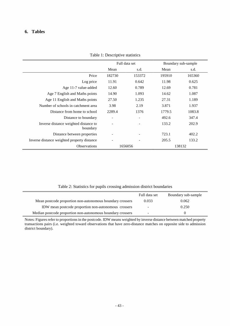
- 43 -

6. Tables

Table 1: Descriptive statistics

Full data set Boundary sub-sample

Mean s.d. Mean s.d.

Price 182730 153372 195910 165360

Log price 11.91 0.642 11.98 0.625

Age 11-7 value-added 12.60 0.789 12.69 0.781

Age 7 English and Maths points 14.90 1.093 14.62 1.087

Age 11 English and Maths points 27.50 1.235 27.31 1.189

Number of schools in catchment area 3.98 2.19 3.871 1.937

Distance from home to school 2289.4 1376 1779.5 1083.8

Distance to boundary - - 492.6 347.4

Inverse distance weighted distance to boundary

- - 133.2 202.9

Distance between properties - - 723.1 402.2

Inverse distance weighted property distance - - 205.5 133.2

Observations 1656056 138132

Table 2: Statistics for pupils crossing admission district boundaries

Full data set Boundary sub-sample

Mean postcode proportion non-autonomous boundary crossers 0.033 0.062

IDW mean postcode proportion non-autonomous crossers - 0.250

Median postcode proportion non-autonomous boundary crossers - 0

Notes: Figures refer to proportions in the postcode. IDW means weighted by inverse distance between matched property transactions pairs (i.e. weighted toward observations that have zero-distance matches on opposite side to admission district boundary).

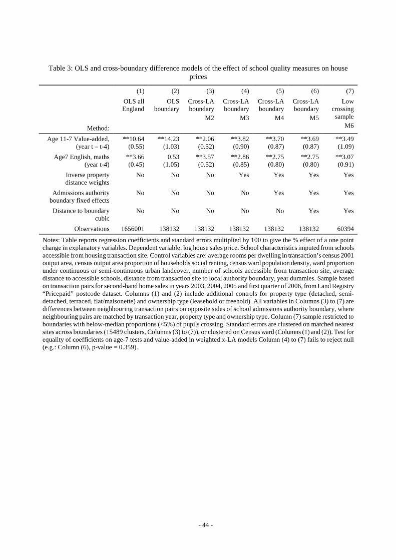
- 44 -

Table 3: OLS and cross-boundary difference models of the effect of school quality measures on house prices

(1) (2) (3) (4) (5) (6) (7)

Method:

OLS all England

OLS boundary

Cross-LA boundary

M2

Cross-LA boundary

M3

Cross-LA boundary

M4

Cross-LA boundary

M5

Low crossing sample

M6

Age 11-7 Value-added, (year t – t-4)

**10.64 (0.55)

**14.23 (1.03)

**2.06 (0.52)

**3.82 (0.90)

**3.70 (0.87)

**3.69 (0.87)

**3.49 (1.09)

Age7 English, maths (year t-4)

**3.66 (0.45)

0.53 (1.05)

**3.57 (0.52)

**2.86 (0.85)

**2.75 (0.80)

**2.75 (0.80)

**3.07 (0.91)

Inverse property distance weights

No No No Yes Yes Yes Yes

Admissions authority boundary fixed effects

No No No No Yes Yes Yes

Distance to boundary cubic

No No No No No Yes Yes

Observations 1656001 138132 138132 138132 138132 138132 60394

Notes: Table reports regression coefficients and standard errors multiplied by 100 to give the % effect of a one point change in explanatory variables. Dependent variable: log house sales price. School characteristics imputed from schools accessible from housing transaction site. Control variables are: average rooms per dwelling in transaction’s census 2001 output area, census output area proportion of households social renting, census ward population density, ward proportion under continuous or semi-continuous urban landcover, number of schools accessible from transaction site, average distance to accessible schools, distance from transaction site to local authority boundary, year dummies. Sample based on transaction pairs for second-hand home sales in years 2003, 2004, 2005 and first quarter of 2006, from Land Registry “Pricepaid” postcode dataset. Columns (1) and (2) include additional controls for property type (detached, semi-detached, terraced, flat/maisonette) and ownership type (leasehold or freehold). All variables in Columns (3) to (7) are differences between neighbouring transaction pairs on opposite sides of school admissions authority boundary, where neighbouring pairs are matched by transaction year, property type and ownership type. Column (7) sample restricted to boundaries with below-median proportions (<5%) of pupils crossing. Standard errors are clustered on matched nearest sites across boundaries (15489 clusters, Columns (3) to (7)), or clustered on Census ward (Columns (1) and (2)). Test for equality of coefficients on age-7 tests and value-added in weighted x-LA models Column (4) to (7) fails to reject null (e.g.: Column (6), p-value = 0.359).

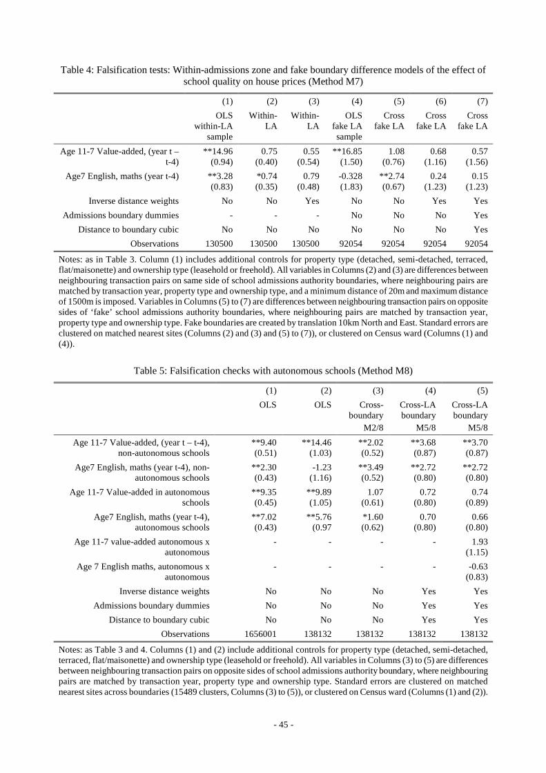
- 45 -

Table 4: Falsification tests: Within-admissions zone and fake boundary difference models of the effect of school quality on house prices (Method M7)

(1) (2) (3) (4) (5) (6) (7)

OLS within-LA

sample

Within-LA

Within-LA

OLS fake LA sample

Cross fake LA

Cross fake LA

Cross fake LA

Age 11-7 Value-added, (year t – t-4)

**14.96 (0.94)

0.75 (0.40)

0.55 (0.54)

**16.85 (1.50)

1.08 (0.76)

0.68 (1.16)

0.57 (1.56)

Age7 English, maths (year t-4) **3.28 (0.83)

*0.74 (0.35)

0.79 (0.48)

-0.328 (1.83)

**2.74 (0.67)

0.24 (1.23)

0.15 (1.23)

Inverse distance weights No No Yes No No Yes Yes

Admissions boundary dummies - - - No No No Yes

Distance to boundary cubic No No No No No No Yes

Observations 130500 130500 130500 92054 92054 92054 92054

Notes: as in Table 3. Column (1) includes additional controls for property type (detached, semi-detached, terraced, flat/maisonette) and ownership type (leasehold or freehold). All variables in Columns (2) and (3) are differences between neighbouring transaction pairs on same side of school admissions authority boundaries, where neighbouring pairs are matched by transaction year, property type and ownership type, and a minimum distance of 20m and maximum distance of 1500m is imposed. Variables in Columns (5) to (7) are differences between neighbouring transaction pairs on opposite sides of ‘fake’ school admissions authority boundaries, where neighbouring pairs are matched by transaction year, property type and ownership type. Fake boundaries are created by translation 10km North and East. Standard errors are clustered on matched nearest sites (Columns (2) and (3) and (5) to (7)), or clustered on Census ward (Columns (1) and (4)).

Table 5: Falsification checks with autonomous schools (Method M8)

(1) (2) (3) (4) (5)

OLS OLS Cross- boundary

M2/8

Cross-LA boundary

M5/8

Cross-LA boundary

M5/8

Age 11-7 Value-added, (year t – t-4), non-autonomous schools

**9.40 (0.51)

**14.46 (1.03)

**2.02 (0.52)

**3.68 (0.87)

**3.70 (0.87)

Age7 English, maths (year t-4), non-autonomous schools

**2.30 (0.43)

-1.23 (1.16)

**3.49 (0.52)

**2.72 (0.80)

**2.72 (0.80)

Age 11-7 Value-added in autonomous schools

**9.35 (0.45)

**9.89 (1.05)

1.07 (0.61)

0.72 (0.80)

0.74 (0.89)

Age7 English, maths (year t-4), autonomous schools

**7.02 (0.43)

**5.76 (0.97

*1.60 (0.62)

0.70 (0.80)

0.66 (0.80)

Age 11-7 value-added autonomous x autonomous

- - - - 1.93 (1.15)

Age 7 English maths, autonomous x autonomous

- - - - -0.63 (0.83)

Inverse distance weights No No No Yes Yes

Admissions boundary dummies No No No Yes Yes

Distance to boundary cubic No No No Yes Yes

Observations 1656001 138132 138132 138132 138132

Notes: as Table 3 and 4. Columns (1) and (2) include additional controls for property type (detached, semi-detached, terraced, flat/maisonette) and ownership type (leasehold or freehold). All variables in Columns (3) to (5) are differences between neighbouring transaction pairs on opposite sides of school admissions authority boundary, where neighbouring pairs are matched by transaction year, property type and ownership type. Standard errors are clustered on matched nearest sites across boundaries (15489 clusters, Columns (3) to (5)), or clustered on Census ward (Columns (1) and (2)).

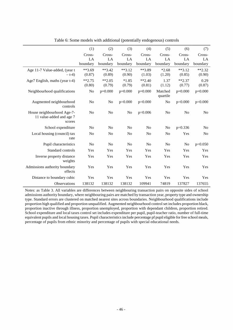
- 46 -

Table 6: Some models with additional (potentially endogenous) controls

(1) (2) (3) (4) (5) (6) (7)

Cross-LA

boundary

Cross-LA

boundary

Cross-LA

boundary

Cross-LA

boundary

Cross-LA

boundary

Cross-LA

boundary

Cross-LA

boundary

Age 11-7 Value-added, (year t – t-4)

**3.69 (0.87)

**3.42 (0.89)

**3.12 (0.90)

**3.89 (1.03)

*2.68 (1.20)

**3.12 (0.85)

**2.32 (0.90)

Age7 English, maths (year t-4) **2.75 (0.80)

**2.05 (0.79)

*1.85 (0.79)

**2.40 (0.81)

1.37 (1.12)

**2.37 (0.77)

0.29 (0.87)

Neighbourhood qualifications No p=0.000 p=0.000 p=0.000 Matched quartile

p=0.000 p=0.000

Augmented neighbourhood controls

No No p=0.000 p=0.000 No p=0.000 p=0.000

House neighbourhood Age-7-11 value-added and age 7

scores

No No No p=0.006 No No No

School expenditure No No No No No p=0.336 No

Local housing (council) tax rate

No No No No No Yes No

Pupil characteristics No No No No No No p=0.050

Standard controls Yes Yes Yes Yes Yes Yes Yes

Inverse property distance weights

Yes Yes Yes Yes Yes Yes Yes

Admissions authority boundary effects

Yes Yes Yes Yes Yes Yes Yes

Distance to boundary cubic Yes Yes Yes Yes Yes Yes Yes

Observations 138132 138132 138132 109941 74819 137827 137655

Notes: as Table 3. All variables are differences between neighbouring transaction pairs on opposite sides of school admissions authority boundary, where neighbouring pairs are matched by transaction year, property type and ownership type. Standard errors are clustered on matched nearest sites across boundaries. Neighbourhood qualifications include proportion high qualified and proportion unqualified. Augmented neighbourhood control set includes proportion black, proportion inactive through illness, proportion unemployed, proportion with dependant children, proportion retired. School expenditure and local taxes control set includes expenditure per pupil, pupil-teacher ratio, number of full-time equivalent pupils and local housing taxes. Pupil characteristics include percentage pf pupil eligible for free school meals, percentage of pupils from ethnic minority and percentage of pupils with special educational needs.

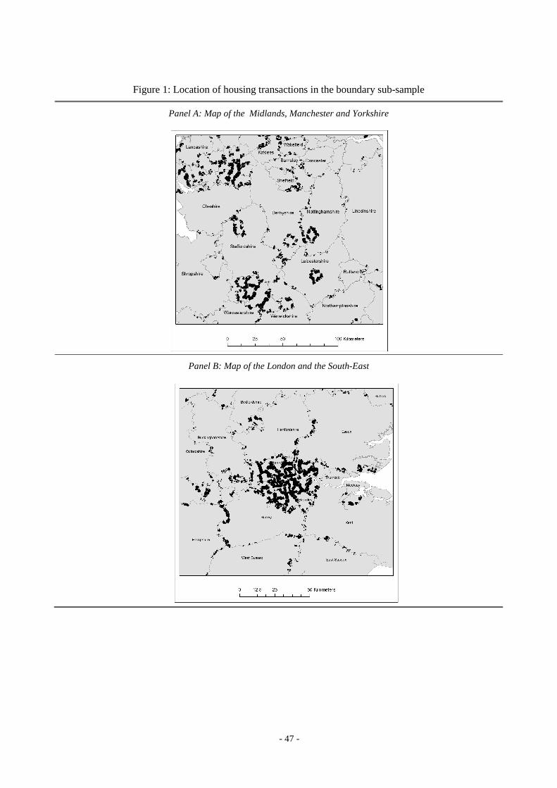
- 47 -

Figure 1: Location of housing transactions in the boundary sub-sample

Panel A: Map of the Midlands, Manchester and Yorkshire

Panel B: Map of the London and the South-East

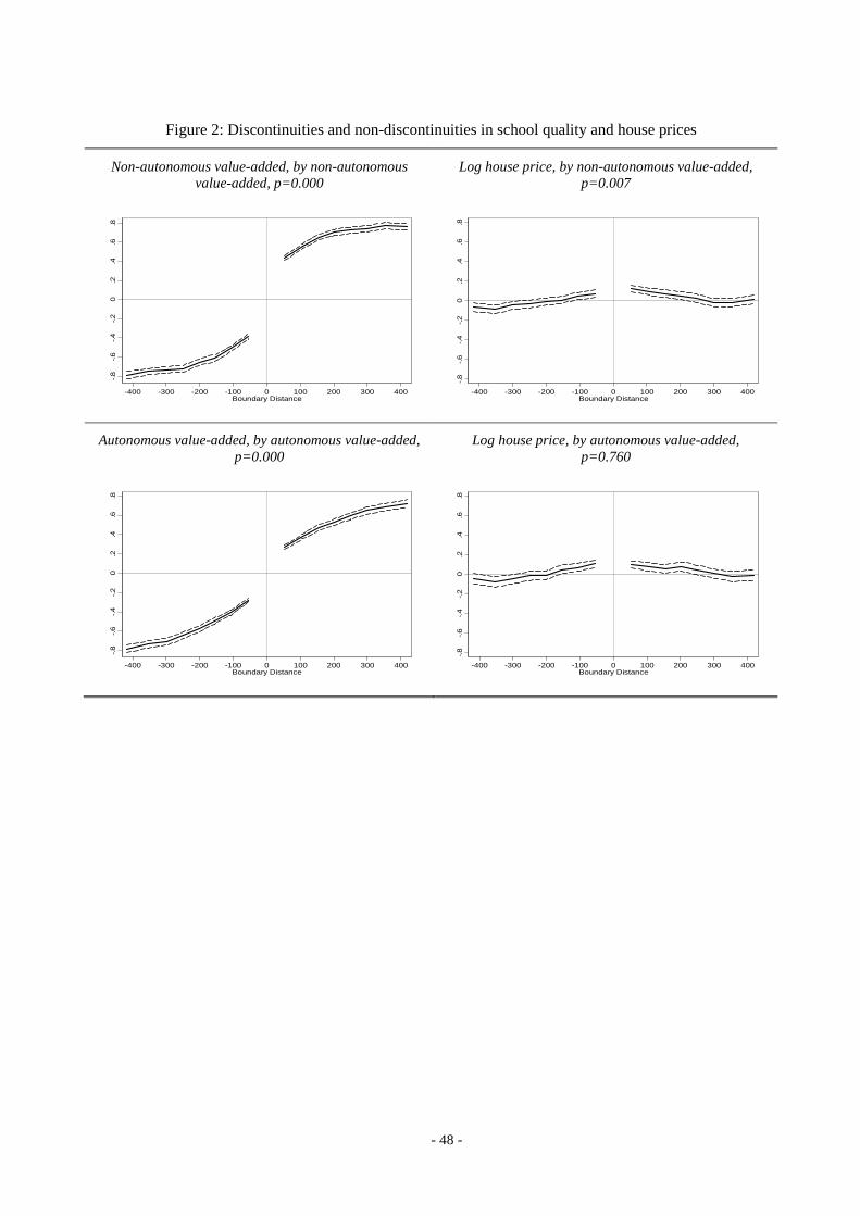
- 48 -

Figure 2: Discontinuities and non-discontinuities in school quality and house prices

Non-autonomous value-added, by non-autonomous value-added, p=0.000

Log house price, by non-autonomous value-added, p=0.007

-.8

-.6

-.4

-.2

0.2

.4.6

.8

-400 -300 -200 -100 0 100 200 300 400Boundary Distance

-.8

-.6

-.4

-.2

0.2

.4.6

.8

-400 -300 -200 -100 0 100 200 300 400Boundary Distance

Autonomous value-added, by autonomous value-added, p=0.000

Log house price, by autonomous value-added, p=0.760

-.8

-.6

-.4

-.2

0.2

.4.6

.8

-400 -300 -200 -100 0 100 200 300 400Boundary Distance

-.8

-.6

-.4

-.2

0.2

.4.6

.8

-400 -300 -200 -100 0 100 200 300 400Boundary Distance

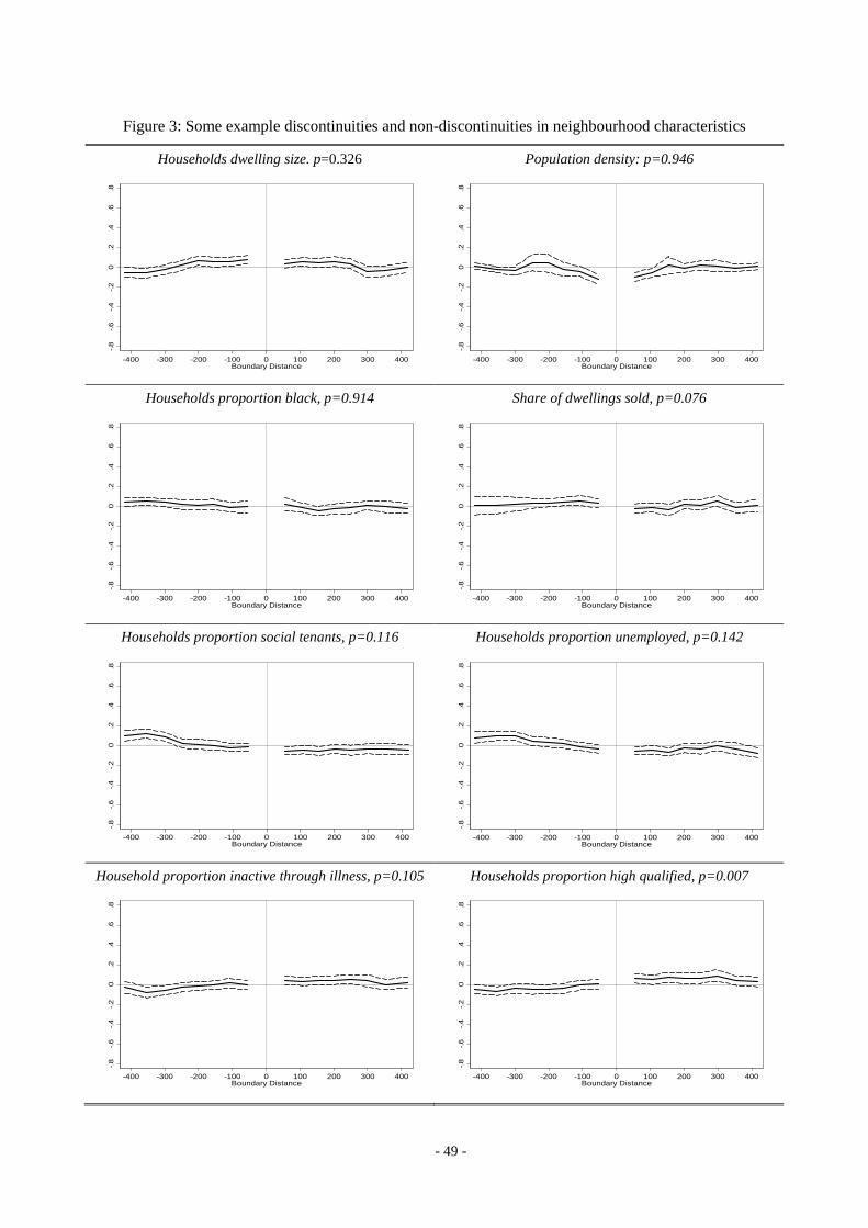
- 49 -

Figure 3: Some example discontinuities and non-discontinuities in neighbourhood characteristics

Households dwelling size. p=0.326 Population density: p=0.946

-.8

-.6

-.4

-.2

0.2

.4.6

.8

-400 -300 -200 -100 0 100 200 300 400Boundary Distance

-.8

-.6

-.4

-.2

0.2

.4.6

.8

-400 -300 -200 -100 0 100 200 300 400Boundary Distance

Households proportion black, p=0.914 Share of dwellings sold, p=0.076

-.8

-.6

-.4

-.2

0.2

.4.6

.8

-400 -300 -200 -100 0 100 200 300 400Boundary Distance

-.8

-.6

-.4

-.2

0.2

.4.6

.8

-400 -300 -200 -100 0 100 200 300 400Boundary Distance

Households proportion social tenants, p=0.116 Households proportion unemployed, p=0.142

-.8

-.6

-.4

-.2

0.2

.4.6

.8

-400 -300 -200 -100 0 100 200 300 400Boundary Distance

-.8

-.6

-.4

-.2

0.2

.4.6

.8

-400 -300 -200 -100 0 100 200 300 400Boundary Distance

Household proportion inactive through illness, p=0.105 Households proportion high qualified, p=0.007

-.8

-.6

-.4

-.2

0.2

.4.6

.8

-400 -300 -200 -100 0 100 200 300 400Boundary Distance

-.8

-.6

-.4

-.2

0.2

.4.6

.8

-400 -300 -200 -100 0 100 200 300 400Boundary Distance