electrical and biomedical 4bi6 statistical pattern

Electrical and Biomedical 4BI6Project Proposal

Statistical Pattern Recognition Methods Applied toEvoked Electroencephalogram Data in Depressed Patients

by

Jason O'Reilly(0648417)

Department of Electrical and Computer EngineeringFaculty Advisors: Dr. H. de Bruin and Dr. J. Reilly

Electrical and Biomedical Engineering Project ReportSubmitted in partial fulfillment of the requirements

for the Bachelor of Engineering

McMaster UniversityHamilton, Ontario, Canada

April 23, 2010

1

I . ABSTRACT

Currently there exist a great deal of medication to deal with various mental disorders. Many of

these medications serve similar purposes though only a select few work for a given individual. It

can take several weeks to assess if any given medication is even working effectively. The purpose

of this project is to develop an objective approach to diagnosing and more accurately treating

various mental disorders with medications. To accomplish this one can observe relationships

between surface currents of the brain and the patients mental disorder through statistical pattern

recognition methods and appropriately assign a specific treatment using data a psychologist

could not observe. The task has high computational requirements and made use of the McMaster

electrical engineering grid. A framework to manipulate gigabytes of EEG data was established.

A method to obtain features necessary was coded into the framework. Conducting a literary

review of the field showed many similar depression calculations. Based on these depression

feature calculations, an EEG analysis framework was established to easily obtain a number of

studied features. Feature selection was used to find features which discriminate between classes.

These features were then input into an support vector machine creating a classifier specifically

designed for depression separation. A test data set of normals was used to perform relevant

depression calculations including band powers, inter-hemispheric power ratios and coherences

between all channel among other prominent calculations common throughout the EEG depression

field. Results of the system were then analyzed to ensure accuracy and meaningfulness.

2

II . ACKNOWLEDGMENTS

I would like to thank Dr. J. Reilly, Dr. H. de Bruin and Ahmad Khodaryari-Rostamabad for

their contributions to this project. I have learnt a great deal from them. Without sharing their

knowledge and experience I would not have known where to being this project. Dr. T. Greenlay

also provided guidance teaching me how to use the McMaster ECEgrid. The assistance was

greatly appreciated.

3

III . TABLE OF CONTENTS

CONTENTS

i ABSTRACT 1

ii ACKNOWLEDGMENTS 2

iii TABLE OF CONTENTS 3

iv LIST OF FIGURES 5

v LIST OF TABLES 6

1 Introduction 7

2 Objectives 11

2-A Handling the Data . . . . . . . . . . . . . . . . . . . . . . . . . . . . . . . 11

2-B Storing the Data . . . . . . . . . . . . . . . . . . . . . . . . . . . . . . . . 11

2-C Functions . . . . . . . . . . . . . . . . . . . . . . . . . . . . . . . . . . . . 11

2-D Learning Machines . . . . . . . . . . . . . . . . . . . . . . . . . . . . . . 12

2-E Analysis . . . . . . . . . . . . . . . . . . . . . . . . . . . . . . . . . . . . 12

3 Literature Review 13

4 Design and Experimental Procedure 16

4-A Coherence . . . . . . . . . . . . . . . . . . . . . . . . . . . . . . . . . . . 16

4-B Coherence Averaging . . . . . . . . . . . . . . . . . . . . . . . . . . . . . 18

4-C Power Averaging . . . . . . . . . . . . . . . . . . . . . . . . . . . . . . . 19

4-D Power Ratios . . . . . . . . . . . . . . . . . . . . . . . . . . . . . . . . . . 20

4-E Coherence Storage . . . . . . . . . . . . . . . . . . . . . . . . . . . . . . . 20

4-F Frequency Feature Matrix . . . . . . . . . . . . . . . . . . . . . . . . . .. 21

4-G Power Feature Matrix . . . . . . . . . . . . . . . . . . . . . . . . . . . . . 21

4-H Power Ratio Feature Matrix . . . . . . . . . . . . . . . . . . . . . . . . . .22

5 Results and Discussion 23

4

6 Conclusions 28

6-A Recommendations . . . . . . . . . . . . . . . . . . . . . . . . . . . . . . . 28

7 Appendices 29

7-A Coherence Function . . . . . . . . . . . . . . . . . . . . . . . . . . . . . . 29

7-B Average Coherence Function . . . . . . . . . . . . . . . . . . . . . . . . .29

7-C Stored Coherence Function . . . . . . . . . . . . . . . . . . . . . . . . . .30

7-D Stored Power Function . . . . . . . . . . . . . . . . . . . . . . . . . . . . 31

7-E Power Ratio Function . . . . . . . . . . . . . . . . . . . . . . . . . . . . . 31

7-F Save Coherences Function . . . . . . . . . . . . . . . . . . . . . . . . . . 32

7-G Frequency Feature Matrix . . . . . . . . . . . . . . . . . . . . . . . . . .. 32

7-H Power Feature Matrix . . . . . . . . . . . . . . . . . . . . . . . . . . . . . 33

7-I Power Ratio Feature Matrix . . . . . . . . . . . . . . . . . . . . . . . . . .34

7-J SVMlight Conversion M File . . . . . . . . . . . . . . . . . . . . . . . . . 35

8 References 37

References 37

9 Vita 38

5

IV. LIST OF FIGURES

L IST OF FIGURES

1 The ion fluxes in the extracellular space are of paramount significance in the

generation of field potentials [7].. . . . . . . . . . . . . . . . . . . . .. . . . . . . 7

2 During EPSP and IPSP, ionic current flows occur through as well as along the

neuronal membrane, as shown by arrows. The density of + and - signs indicate

the polarization of the subsynaptic (dark area) as well as that of the postsynaptic

membrane during synaptic activation [7]. . . . . . . . . . . . . . . .. . . . . . . . 8

3 Features x1 and x2 contain little information of class separation. Feature x3 shows

clear separation of the classes [6]. . . . . . . . . . . . . . . . . . . . .. . . . . . . 9

4 Raw Data: Raw EEG data from channels O1, F1, and T1. Showing 1000 samples

of 43000 sampled at 205 Hz. . . . . . . . . . . . . . . . . . . . . . . . . . . . . .. 16

5 Cross-Correlation: Cross-correlation of proximal EEG channels shows near 1 cor-

relation at tau equals 0. . . . . . . . . . . . . . . . . . . . . . . . . . . . . . .. . . 17

6 Coherence: Coherence calculations between proixmal channels Fz and F1 share

delta and alpha power. . . . . . . . . . . . . . . . . . . . . . . . . . . . . . . . .. 18

7 Distant Coherence: Coherence calculations between distantchannels. . . . . . . . . 23

8 Average Coherence: Coherence calculations between proximal channels Fz and F1.

The coherence is averaged over 6 trials, three eyes open and three eyes closed. . . 24

9 Left Hemispheric Power: Left hemisphere channel powers indelta, theta, alpha and

beta bands. Four rows contains one channel of information. The last two bands of

the last channel, rows 35 and 36 are not shown. The first 11 patients can be seen.

Power spectral densities of channels X1, T3, F7, T5, F3, C3, P3, and O1 are shown. 25

10 Right Hemispheric Power: Right hemisphere channel powers in delta, theta, alpha

and beta bands. Four rows contains one channel of information. The last two bands

of the last channel, rows 35 and 36 are not shown. The first 11 patients can be

seen. Power spectral densities of channels X1, T3, F7, T5, F3, C3, P3, and O1 are

shown. . . . . . . . . . . . . . . . . . . . . . . . . . . . . . . . . . . . . . . . . . . 26

11 Cross Coherence: Cross coherence across hemispheres. Cross Power spectral den-

sities of channels X, T, F, T, F, C, P, and O are shown. . . . . . . . . .. . . . . . 27

6

V. LIST OF TABLES

L IST OF TABLES

I Frequency Band Average Powers . . . . . . . . . . . . . . . . . . . . . . . . .. . . 20

7

1. INTRODUCTION

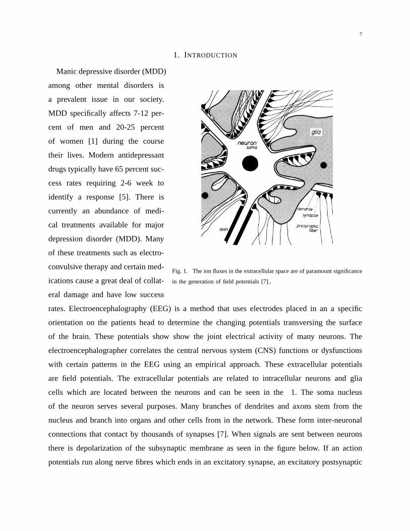
Fig. 1. The ion fluxes in the extracellular space are of paramount significance

in the generation of field potentials [7]..

Manic depressive disorder (MDD)

among other mental disorders is

a prevalent issue in our society.

MDD specifically affects 7-12 per-

cent of men and 20-25 percent

of women [1] during the course

their lives. Modern antidepressant

drugs typically have 65 percent suc-

cess rates requiring 2-6 week to

identify a response [5]. There is

currently an abundance of medi-

cal treatments available for major

depression disorder (MDD). Many

of these treatments such as electro-

convulsive therapy and certain med-

ications cause a great deal of collat-

eral damage and have low success

rates. Electroencephalography (EEG) is a method that uses electrodes placed in an a specific

orientation on the patients head to determine the changing potentials transversing the surface

of the brain. These potentials show show the joint electrical activity of many neurons. The

electroencephalographer correlates the central nervous system (CNS) functions or dysfunctions

with certain patterns in the EEG using an empirical approach. These extracellular potentials

are field potentials. The extracellular potentials are related to intracellular neurons and glia

cells which are located between the neurons and can be seen inthe 1. The soma nucleus

of the neuron serves several purposes. Many branches of dendrites and axons stem from the

nucleus and branch into organs and other cells from in the network. These form inter-neuronal

connections that contact by thousands of synapses [7]. When signals are sent between neurons

there is depolarization of the subsynaptic membrane as seenin the figure below. If an action

potentials run along nerve fibres which ends in an excitatorysynapse, an excitatory postsynaptic

8

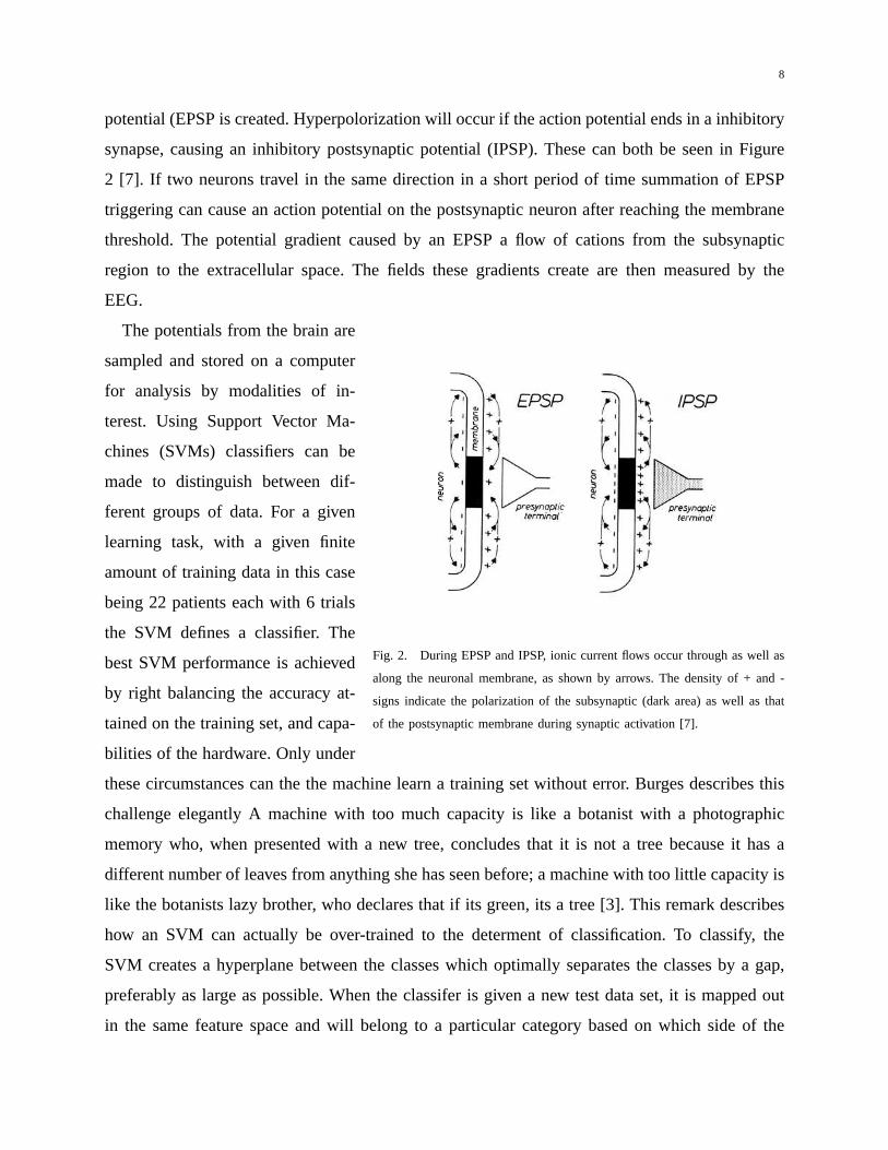
potential (EPSP is created. Hyperpolorization will occur if the action potential ends in a inhibitory

synapse, causing an inhibitory postsynaptic potential (IPSP). These can both be seen in Figure

2 [7]. If two neurons travel in the same direction in a short period of time summation of EPSP

triggering can cause an action potential on the postsynaptic neuron after reaching the membrane

threshold. The potential gradient caused by an EPSP a flow of cations from the subsynaptic

region to the extracellular space. The fields these gradients create are then measured by the

EEG.

Fig. 2. During EPSP and IPSP, ionic current flows occur through as well as

along the neuronal membrane, as shown by arrows. The density of + and -

signs indicate the polarization of the subsynaptic (dark area) as well as that

of the postsynaptic membrane during synaptic activation [7].

The potentials from the brain are

sampled and stored on a computer

for analysis by modalities of in-

terest. Using Support Vector Ma-

chines (SVMs) classifiers can be

made to distinguish between dif-

ferent groups of data. For a given

learning task, with a given finite

amount of training data in this case

being 22 patients each with 6 trials

the SVM defines a classifier. The

best SVM performance is achieved

by right balancing the accuracy at-

tained on the training set, and capa-

bilities of the hardware. Only under

these circumstances can the the machine learn a training setwithout error. Burges describes this

challenge elegantly A machine with too much capacity is likea botanist with a photographic

memory who, when presented with a new tree, concludes that itis not a tree because it has a

different number of leaves from anything she has seen before; a machine with too little capacity is

like the botanists lazy brother, who declares that if its green, its a tree [3]. This remark describes

how an SVM can actually be over-trained to the determent of classification. To classify, the

SVM creates a hyperplane between the classes which optimally separates the classes by a gap,

preferably as large as possible. When the classifer is given anew test data set, it is mapped out

in the same feature space and will belong to a particular category based on which side of the

9

gap the are on. Another key factor is the selection of the features themselves that make up the

mapping. Every feature cannot be selected, the mapping of the data to the feature space with

massive dimensions would result in a machine with poor performance. This is because a set of

hyperplanes for a given SVM are parameterized by the dimensions of the feature matrix [3].

Feature selection can be decomposed into two steps. The feature construction aspect, and the

feature selection. The goal of this is ultimately data reduction to limit storage requirements and

increase algorithm speed. The EEG data is the general data and is not within the scope of the

project to be retrieve or alter the given general data set.

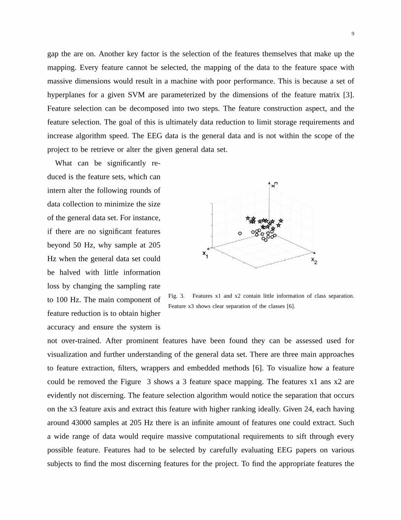
Fig. 3. Features x1 and x2 contain little information of class separation.

Feature x3 shows clear separation of the classes [6].

What can be significantly re-

duced is the feature sets, which can

intern alter the following rounds of

data collection to minimize the size

of the general data set. For instance,

if there are no significant features

beyond 50 Hz, why sample at 205

Hz when the general data set could

be halved with little information

loss by changing the sampling rate

to 100 Hz. The main component of

feature reduction is to obtain higher

accuracy and ensure the system is

not over-trained. After prominent features have been foundthey can be assessed used for

visualization and further understanding of the general data set. There are three main approaches

to feature extraction, filters, wrappers and embedded methods [6]. To visualize how a feature

could be removed the Figure 3 shows a 3 feature space mapping.The features x1 ans x2 are

evidently not discerning. The feature selection algorithmwould notice the separation that occurs

on the x3 feature axis and extract this feature with higher ranking ideally. Given 24, each having

around 43000 samples at 205 Hz there is an infinite amount of features one could extract. Such

a wide range of data would require massive computational requirements to sift through every

possible feature. Features had to be selected by carefully evaluating EEG papers on various

subjects to find the most discerning features for the project. To find the appropriate features the

10

brain must first be examined from a psychologist’s standpoint. One of the pioneers in the EEG

depression field, Davidson [4] found that brain asymmetry isrelated to depression. Davidson’s

finding showed a relationship depression and less activation power in the left frontal cortex when

compared to the right frontal cortex. People found with thisasymmetry were more likely to show

signs of depression which was especially apparent in the alpha power band. Asymmetry studies

are a common theme throughout depression papers, as such a two functions were developed in

Matlab to distinguish power ratios of given frequency bands. Depression features are now being

insistently researched because of the prevalence of depression in society and is detailed in the

literature review.

11

2. OBJECTIVES

The original objective outlined my proposal at the beginning of the year was to use EEG data

to achieve a more accurate and objective description of a patients depression status. In order to

accomplish this, many software components had to be developed or selected to deal with the

shear magnitude of data. The primary objective of the project is quite broad and sub-objectives

were developed throughout the course of the term as a result of unforeseeable circumstances.

A. Handling the Data

Development of a framework to handle the data, allowing one to open and manipulate EEG

data with relative ease was the first objective after literature review had been conducted. There

are twenty-two patients, each having six trials with 24 channels sampled at 205 Hz with 43000

data points per channel. Functions needed to be created to easily access the data. For example

a function had to be created to retrieve patient 12, trial number 3, channel number 5, etc. This

component objective was vital for analysis of the EEG data. After this task was complete, analysis

of the data was to be considered.

B. Storing the Data

After performing some analysis trials on the data, such as Fast Fourier Transforms and corre-

lations the required computational requirements became clear and a new objective was created.

It would be impossible to perform analysis in the desired time frame constantly performing

FFTs and correlations because there were simply to many calculations. The next objective was

deciding the most meaningful data to store to maximize computational speeds but not taking up

ridiculous amounts of disk space at the same time. A balance needed to be established.

C. Functions

While sifting through the papers in the field, many calculations and measurements for depres-

sion and other EEG relationships were found. There were manyequations describing similar

attributes such as asymmetry. A base of functions had to be developed to implement the equations

and allow for future additions was necessary.

12

D. Learning Machines

Once all the appropriate numbers were established from the analysis, the objective was to

implement a learning machine. There are a great deal of statistical pattern recognition and

learning machines available, many of which are open source.Research was conducted to find

the learning machine most suitable for this project. Code forproper formatting had to be done

on the data to be created for inputing to the learning machines.

E. Analysis

The task of analyzing the output of the learning machine and the analysis equations were the

next concern. Individually evaluating which equations created the features that were optimal for

classification. Selection of the correct features can drastically change the accuracy and speed.

13

3. LITERATURE REVIEW

Another measure that was found to be a prominent indication of depression was the Frontal

Brain Asymmetry (FBA) ratio . The formula is as follows [8]:

Where PL is the left alpha power PR is the right alpha power. Thederivation of this formula

is based on the results from a number of studies. The alpha power in the brain is inversely

proportional to mental activity (Davidson, 1988). Thus, ifa person is doing intense mental

arithmetic a small alpha power is observed in that region of the brain, whereas if someone is

mentally inactive in a given region, that region will tend tohave higher alpha power. Thus, the

formula is basically normalizing the left-right difference in brain activity for given left and right

channels. A function was created to obtain this feature for two given channels. Inter-hemispheric

coherence between FP1-FP2, T3-T4, P3-T4, and O1 and O2 in particularly alpha and theta bands

were a common indicator of depression being studied in several papers. The formula used is for

inter-hemispheric coherence was as follows:

Sxy is the cross-spectral density of the two signals. Sxx andXyy are the power spectral density

of each signal by itself. The spectral asymmetry index (SASI) is another key calculation and is

the relative difference in power of two EEG special frequency bands. It is calculated as follows:

14

Wlmn corresponds to the lower frequency density of channels mand n from frequency F1

to F2. Whmn are the higher frequency densities of channels m and n from frequency F3 to F4.

Finally, these are used to calculate the SASI:

Evidently, the power asymmetry between two channels m and n are represented by the SASI

[?]. To obtain a frequency bands ratio with respect to the entire frequency band, the following

calculation is used:

interest with respect to the entire band of measured brain frequency. The normalized densities

can then be used to calculate the inter-hemispheric asymmetry [?]:

15

This is quite similar to the Frontal Brain Asymmetry calculation except the inverse of the

power is not taken and this asymmetry is reflective only of power differences and not cognitive

function at the time of measurement as in FBA. Several papersaddress the There are many

methods currently being implemented to analyze EEG data. Many papers implement analyze

data specifically for EEG purposes. Another segment of papers dealt with detection of early

response to medications. The literature review revealed the broadness of the EEG depression

field.

16

4. DESIGN AND EXPERIMENTAL PROCEDURE

The basis of the overall design are the functions created to manipulate the data. After comple-

tion of each function several tests were performed to ensureit was functional and had meaningful

output. The EEG data itself with no modifications is shown in 4. This shows figure basically

a few arbitrary channels from the occipital, frontal and temporal lobes. This only displaying a

few thousand samples of the 43000 at 205 Hz.

Fig. 4. Raw Data: Raw EEG data from channels O1, F1, and T1. Showing 1000 samples of 43000 sampled at 205 Hz.

The potentials are on the order of microvolts which is expected for EEG signals. The temporal

and frontal lobe can be seen to follow each other more closelygiven their proximity. The occipital

lobe at the back of the heads potential is quite different. This is the raw data the design of the

project is based on. The main functions designed to manipulate the EEG data are now listed.

A. Coherence

function [Xcoh freq] = getCoherence(x1,x2) Inputs: 2 1xN column vectors of EEG data

Outputs: Normalized correlation of channels with size 1x(N-1) and corresponding frequencies

17

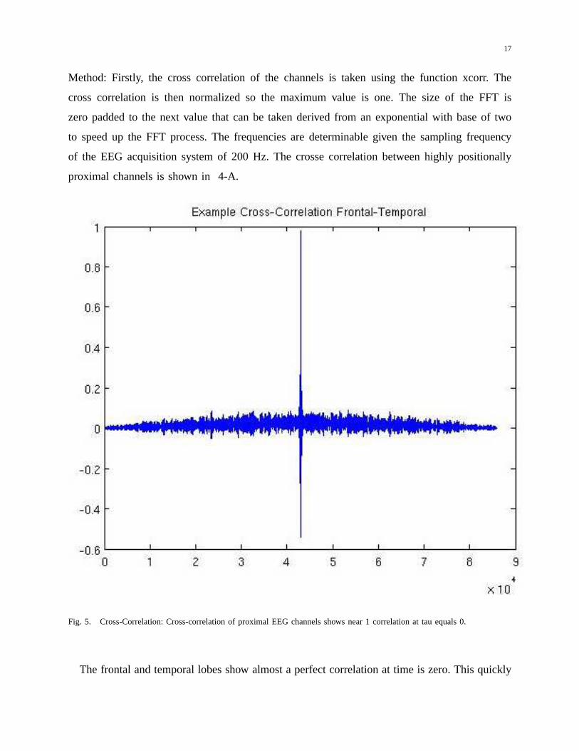
Method: Firstly, the cross correlation of the channels is taken using the function xcorr. The

cross correlation is then normalized so the maximum value isone. The size of the FFT is

zero padded to the next value that can be taken derived from anexponential with base of two

to speed up the FFT process. The frequencies are determinable given the sampling frequency

of the EEG acquisition system of 200 Hz. The crosse correlation between highly positionally

proximal channels is shown in 4-A.

Fig. 5. Cross-Correlation: Cross-correlation of proximal EEG channels shows near 1 correlation at tau equals 0.

The frontal and temporal lobes show almost a perfect correlation at time is zero. This quickly

18

drops off steeply after. The correlation is normalized. Taking the FFT of the normalized corre-

lation using this function yielded the following output:

Fig. 6. Coherence: Coherence calculations between proixmal channels Fz and F1 share delta and alpha power.

Image 4-A shows the coherence between proximal channels Fz and F1. The FFT can show

data up to around 100 Hz, half the sampling frequency. This coherence shows only the first 20

or so hertz. A strong delta power can be seen between 0.5-4 Hz.In addition to this alpha band

activity can be seen in the 8-14 Hz range. Beta and theta bands appear relatively inactive in this

segment. The fact that there was a physiological meaning of the data indicated the coherence

was working properly.

B. Coherence Averaging

function [AVGcoh freq] = getAveragedCoherence(patient,x1,x2) Inputs: The number corre-

sponding to the patients of interest and channels containing EEG data Outputs: Averaged cor-

19

relation size 1x(N-1) and corresponding frequencies. Method: Opens all six EEG data files

including EO/EC and retrieves desired channels x1 and x2. Itcalls function (1) six times and

averages the results. Purpose: This is an important step to minimize error. Notes: There was also

a similar function with similar output created except it uses the saved average frequencies as

the input to decrease computational time.

C. Power Averaging

function AvgPow = getSavedAvgPower(patient,x1,x2,freq0,freq1) Inputs: The patient number

from 1-22 and the channels of interest. Freq0 and freq1 represent the upper and lower bounds

of the frequencies that average power is calculated over. Method: Opens the saved coherence

data which can be also interpreted as the power spectral density functions (PSDs) between the

two channels. The power is then just the integral from freq0 to freq1. Since the data points are

discrete an approximation had to be made to calculate the area under the curve. A fast way to

solve for the area was to take each discrete data points magnitude within the range freq0 to

freq1 and multiple it by on frequency interval and sum the result. Using this method there will

clearly be some overlap over the boundaries by half a frequency interval on each side in the

band, but the size of a frequency increment negligible compared to the range between freq0 and

freq1. This yields a relatively accurate method of efficiently calculating the power. After using

this estimate it became apparent that one could just as well sum all the data points and multiply

it by one frequency interval which could simplify the process. Another realization was then

made that multiplying by some arbitrary constant every timewas also useless because it does

not change the relative relationship between the values andthe feature selection algorithm would

treat it the same without multiplying the discrete points bythe frequency interval. Finally, it was

decided just to sum the magnitude of the data points because to the support vector machine it

is all the same so long as all eigenvalue values are proportional. Purpose: Power was shown to

be an important feature in many applications during the literature review. It can be used to find

powers of the alpha, beta, theta and gamma brain waves. It canalso be used in calculation of

power ratios.

20

D. Power Ratios

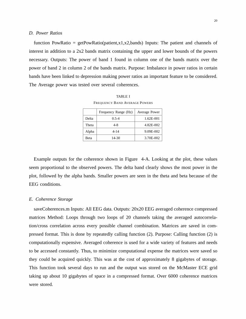
function PowRatio = getPowRatio(patient,x1,x2,bands) Inputs: The patient and channels of

interest in addition to a 2x2 bands matrix containing the upper and lower bounds of the powers

necessary. Outputs: The power of band 1 found in column one ofthe bands matrix over the

power of band 2 in column 2 of the bands matrix. Purpose: Imbalance in power ratios in certain

bands have been linked to depression making power ratios an important feature to be considered.

The Average power was tested over several coherences.

TABLE I

FREQUENCYBAND AVERAGE POWERS

Frequency Range (Hz) Average Power

Delta 0.5-4 1.62E-001

Theta 4-8 4.82E-002

Alpha 4-14 9.09E-002

Beta 14-30 3.70E-002

Example outputs for the coherence shown in Figure 4-A. Looking at the plot, these values

seem proportional to the observed powers. The delta band clearly shows the most power in the

plot, followed by the alpha bands. Smaller powers are seen inthe theta and beta because of the

EEG conditions.

E. Coherence Storage

saveCoherences.m Inputs: All EEG data. Outputs: 20x20 EEG averaged coherence compressed

matrices Method: Loops through two loops of 20 channels taking the averaged autocorrela-

tion/cross correlation across every possible channel combination. Matrices are saved in com-

pressed format. This is done by repeatedly calling function(2). Purpose: Calling function (2) is

computationally expensive. Averaged coherence is used fora wide variety of features and needs

to be accessed constantly. Thus, to minimize computationalexpense the matrices were saved so

they could be acquired quickly. This was at the cost of approximately 8 gigabytes of storage.

This function took several days to run and the output was stored on the McMaster ECE grid

taking up about 10 gigabytes of space in a compressed format.Over 6000 coherence matrices

were stored.

21

F. Frequency Feature Matrix

function m = freqFeatMat(x1,x2,freqs) Inputs: Arrays of channels and frequencies of inter-

est. Outputs: A coherence frequency feature matrix with rows sized number of size nChan-

nels*nFrequencies of interest and 22 columns, one for each patient. Method: Loops through

each channel combination in arrays x1 and x2. Select frequencies in the freqs array are taken

from the coherence of each channel combination and stored under the patients column. Each

patient is looped until all 22 columns are filled with coherence frequency data. Purpose: Creates

a feature matrix of selected frequencies and channels to be input into a feature matrix or feature

selection algorithm. Certain brain frequencies can be correlated to depression among other things.

This function was the basis of creating other feature matrices but was not used itself in practice

because at each discrete frequency point is subject to too much noise. Averaging over large

frequencies tends to be a more accurate representation. In addition, with 43000 data points

each with an individual frequency feature per channel, a frequency feature matrix containing all

possible frequencies could not be implemented giving the volume of data. The feature matrix

would be to massive for practical use though it would be possible with more computational

power. With infinite computational power this would likely give the most discerning features

but because computational power is limited other forms of feature matrices must be designed to

meet the requirements.

G. Power Feature Matrix

function m = powFeatMat(x1,x2) Inputs: Arrays of channels of interest. The frequency band

input was restricted to alpha, beta, theta and gamma brain power calculations. Outputs: A power

feature matrix with rows sized number of size nChannels*4 and22 columns. Four brain wave

bands are considered. Method: Goes through each channel array opening the saved coherence

values. Calculates the power in the brain wave bands for each channel and saves it into the patients

column and corresponding feature row. This process is repeated for each patient. Purpose: Creates

a feature matrix of brain wave powers. These have shown to be important features to analyze

throughout the literature review.

22

H. Power Ratio Feature Matrix

function m = powRatioFeatMat(x1,x2, bands) Inputs: Arrays of channels of interest. In this

case frequencies bands can be modified by the user. Only two bands can be input in the bands

array which is a 2x2 matrix containing the upper and lower bounds of the bands. Outputs: A

matrix of size nChannels x nPatients. A the power for each bandis calculated an the power of

first band in column 1 of the input band matrix is divided by thepower in the column 2 band.

Method: Opens saved coherence values and calls the getPowRatio function to obtain the values

of the feature matrix. Purpose: Power ratios features have been shown to relate to depression.

23

5. RESULTS AND DISCUSSION

Previously in Figure 4-A the coherence between proximal channels were shown. The alpha

and delta powers were most prominent in this scenario. To further test the system and the

accuracy of the data distant coherences were also measured.Coherence between F1 and O2 are

shown in the Figure 5.

Fig. 7. Distant Coherence: Coherence calculations between distant channels.

Far less activation in the delta bands is apparent. Some relationship can still be seen in the

alpha band however. This may be an indication that alpha waves are being transmitted throughout

the brain to a greater extent than the delta waves. Once againthe other theta and beta bands are

not active at all. Running a few more trials the coherence getCoherence function was working

for all patients and channels with an exception in patient 13where there was a data fault that

caused the program to crash.

The average coherence function was also tested for its reliability. The output of this function

for proximal channels Fz and F1 are can be seen below in Figure5.

As one might expect. Averaging reduces the magnitude to a considerable degree. This is as

24

Fig. 8. Average Coherence: Coherence calculations between proximal channels Fz and F1. The coherence is averaged over 6

trials, three eyes open and three eyes closed.

a result of the high frequencies components being averaged out or smoothed. The averaging

appears to have a similar effect to a lowpass filter that removes high frequency components to

some degree. The averaging is done across six trials with three samples of eyes open and three

eyes closed. There is no discrimination between these casesin the software framework currently

because no papers regarding depression covered the topic and it was assumed not significant. If

a paper was published that found differences in classification of depressed patients when their

eyes are open versus when their eyes are closed this would need to be considered and would

require minor changes to the coding. The output of this function appears to make physiological

sense and after several trial appeared to be working smoothly.

To test the system several calculations seen commonly throughout the papers were imple-

mented with the software framework established. First powers in the left hemisphere were

measured. These are seen below in Figure??. Nine channels were measured in four frequency

bands. The last two bands of the last channel are not shown.

The powers all appear around the E-4 and E-5 level which is roughly speaking the order of

magnitude to be expected. The first row measuring channel X1 seems to be similar across all

11 patients in terms of magnitude. Many other rows show a widevariety of values containing

25

Fig. 9. Left Hemispheric Power: Left hemisphere channel powers indelta, theta, alpha and beta bands. Four rows contains

one channel of information. The last two bands of the last channel, rows 35 and 36 are not shown. The first 11 patients can be

seen. Power spectral densities of channels X1, T3, F7, T5, F3, C3, P3, and O1 are shown.

desired features that could potentially seperate depressed patients from normals. There appears

to be no large sources of high magnitude noise anywhere throughout the power feature matrix

indicating the general data set was accurately obtained. This matrix can now be compared to

the same bands and channels on the right side of the hemisphere seen in Figure 5.

Comparing the values between the charts some relationships are immediately apparent. Mag-

nitudes in differing rows tend to vary to a similar degree. Inaddition, the variances on the rows

appear similar in both hemispheres which makes physiological sense. For example, comparing

the first rows of left and right hemispheres, the first rows magnitude slightly changes overall

between hemispheres, showing more power generally in the left. These are normal patients, yet

the magnitudes in the left hemisphere appears slightly greater indicating asymmetry in normal

patients. It is a possibility that the left side of the brain shows slightly more activity even in normal

patients on average. In creating a system that identifies depression such natural asymmetries

would need to be accounted for. This magnitude differences may have also been introduced in

26

Fig. 10. Right Hemispheric Power: Right hemisphere channel powersin delta, theta, alpha and beta bands. Four rows contains

one channel of information. The last two bands of the last channel, rows 35 and 36 are not shown. The first 11 patients can be

seen. Power spectral densities of channels X1, T3, F7, T5, F3, C3, P3, and O1 are shown.

the measuring phase of the general EEG data. Plotting the features clearly shows relationships

between channels and can be seen in Figure 5.

Interestingly, the features of each patient seem to follow asimilar but not exact pattern. Power

spikes are generally seen in the same regions for all patients. Small differences in the magnitudes

and phase of these spikes can be noticed and an the support vector machine will classify based

on these types of differences. As part of the framework, codewas created to concatenate these

feature matrices and to be input into a support vector machine. The SVM used for this project

was SVMlight which requires a particular input format. The conversion from a feature matrix to

an SVMlight input matrix code can be seen in the appendices. Separation was performed based

on gender, and the SVMlight was able to distinguish gender with low accuracy. More details on

this separation was excluded because it is not in the vein of the report concerning depression.

Seperation by gender is a topic of a different nature. Genderseperation was done only to show

the system working and the conversions had been done correctly. After this seperation was

27

0 5 10 15 20 25 30 35 400

1

2

x 10−4 Feature Plot: Inter−hemispheric Cross−Coherences

Fig. 11. Cross Coherence: Cross coherence across hemispheres. Cross Power spectral densities of channels X, T, F, T, F, C,

P, and O are shown.

completed and the SVM was shown to be working, the system was ready for inputing massive

feature matrices from depressed patients.

28

6. CONCLUSIONS

In conclusion, the software framework appears to be workingadequately. The system can

easily implement features discussed in the papers with onlyslight modifications to the code. The

storage of coherences across all possible channel combinations drastically speeds up the process

of analyzing the data at the cost of roughly 10 gigabytes of space. The shear volume of the data

requires usage of a computational grid and cannot possibly be completed on a home desktop

computer in a reasonable time frame. The initial coherencescalculated on individual trials show

large amounts of high frequency content and are not suitablefor direct usage. Averaging functions

across the six trials were made to deal with this issue and allaverage coherences were calculated

and saved with the usage of the McMaster ECE grid. The averageswere shown to work similar

to lowpass filters, reducing the magnitudes of the signals but increasing the signal to noise ratio.

All functions were tested through creation of the final feature matrices to be input into the SVM.

These included frequency, power, and power ratio feature matrices. A variety of of functions were

assembled to create these feature matrices. These functions easily implemented inter-hemispheric

related features such as brain asymmetries which were even observed in normal patients on

several channels. Finally, conversion functions were created to transfer the feature matrices into

SVMlight. The system is essentially ready for implementation on depressed patients. The wide

variation of readings in normal patients shows depression seperation would be a difficult task.

With further research, data and optimization of machines the seperation of depressed individuals

seems promising.

A. Recommendations

Recommendations for further work would be in the area of creating a custom feature selection

and support vector machine specifically for the purposed of depression. The parameters of the

SVM can also be tweaked along with the number of features input to increase accuracy. The

framework potentially could include a method by which it automatically increases or decreases

parameters until maximum separation in the feature space occurs. Computational requirements

would be quite high for such an algorithm and methods such as the Monte Carlo algorithm

would need to be used to find the most suitable parameters. In addition to this, more papers

could be researched and their features tested to increase the accuracy of the system.

29

7. APPENDICES

A. Coherence Function

function [Xcoh,freq] = getCoherence(x1,x2)

X= xcorr(x1,x2,’coeff’); //normalized cross-correlation

Ts = 0.0049;

Fs = 1/Ts; //pre-definded, 205 Hz

L = size(X);

L = L(1);

NFFT = 2nextpow2(L); // Next power of 2 from length of y

Xcoh = abs(fft(X,NFFT)/L);

freq = Fs/2*linspace(0,1,NFFT/2+1); // f size is around 32769

//Xcoh = Xcoh(1:30000);

freq = freq(1:30000);//only considering to 30000 point (46.7 Hz)

end

B. Average Coherence Function

function [AVGcoh freq] = getAveragedCoherence(patient,e1,e2)

//channels only from 1 to 24

root = ’/home/oreillj/dropbox/HamNorms0/’;

load(’patients.mat’);

//open raw data files

data1 = dlmread(strcat(root,patients(patient).name,’/ECV01R01.txt’),’⁀’,2,3);






//take desired columns

x1 = data1.data(:,e1);

30












//obtain coherences

[X1 freq] = getCoherence(x1,x11);






//averaging

AVGcoh = (X1+X2+X3+X4+X5+X6)/6;

f = freq;

end

C. Stored Coherence Function

function AvgCoh = getSavedAvgCoh(patient,e1,e2)

cd(’/home/surf/Documents/School/4BI6/HamNorms0/’);

filename = [ ’AvgCoh ’ num2str(patient) ’ ’ num2str(e1) ’ ’ num2str(e2) ’.mat’ ];

AvgCoh = load(filename);

31

AvgCoh = AvgCoh.m;

end

D. Stored Power Function

function AvgPow = getSavedAvgPower(patient,e1,e2,freq0,freq1)

m = getSavedAvgCoh(patient,e1,e2);

onef = 642.2826; //one step in Hz

n0 = round(freq0*onef);

n1 = round(freq1*onef);

N = n1-n0;

Power = 0;cohfunctionAp

for k=n0:n1

Power = Power + m(k);

end

AvgPow = Power;

end

E. Power Ratio Function

function PowRatio = getPowRatio(patient,e1,e2,bands)

// average pow e1 over e2

freq0 = bands(1,1);

freq1 = bands(2,1);

freq2 = bands(1,2);

freq3 = bands(2,2);

pow0 = getSavedAvgPower(patient,e1,e1,freq0,freq1);

pow1 = getSavedAvgPower(patient,e2,e2,freq2,freq3);

PowRatio = pow0/pow1;

end

32

F. Save Coherences Function

for k = 1:22 //pateints

for h = 1:24 //all cross-channel relations

for t = 1:24

if(k == 13)

continue;

end

if(t==h)

continue;

end

m = getAveragedCoherence(k,h,t);

cd(’/home/oreillj/Coherence’);

if(t¿h)

filename = [ ’AvgCoh ’ num2str(k) ’ ’ num2str(h) ’ ’ num2str(t) ’.mat’ ];

end

if(t¡h)

filename = [ ’AvgCoh ’ num2str(k) ’ ’ num2str(t) ’ ’ num2str(h) ’.mat’ ];

end

save(filename, ’m’);

end

end

end

G. Frequency Feature Matrix

function m = freqFeatMat(e1,e2,freqs)

nChannels = length(e1);

nPatients = 22;

nFreqs = length(freqs);

33

nRows = nFreqs*nChannels;

nCol = nPatients;

m = zeros(nRows,nPatients);// 13 col will need removal

for k = 1:nPatients

if(k == 13) // 13 is useless for now

continue;

end

for s = 1:nChannels

for q = 1:nFreqs

e11 = e1(s);

e22 = e2(s);

freq = freqs(q);

cRow = s*q; //current channel times freq of interest

cCol = k; // current column is current patient

val = getSavedAvgCohatF(k,e11,e22,freq);

m(cRow,cCol) = val;

end

end

end

end

H. Power Feature Matrix

function m = powFeatMat(e1,e2)

bands = [.5 4 8 14; 4 8 14 30]; // the delta theta alpha beta bands

nBands = 4;// for now the bands are locked as these


nPatients = 22;

nRows = nBands*nChannels;

nCol = nPatients;

34


for k = 1:nPatients

cRow = 1;

cCol = k; // current column is current patient

for s = 1:nChannels

for q = 1:nBands

e11 = e1(s);

e22 = e2(s);

lowFreq = bands(1,q);

highFreq = bands(2,q);

val = getSavedAvgPower(k,e11,e22,lowFreq,highFreq);

m(cRow,cCol) = val;

cRow = cRow +1;

end

end

end

end

I. Power Ratio Feature Matrix

function m = powRatioFeatMat(e1,e2, bands)


nPatients = 22;

nCol = nPatients;

nRows = nChannels;


for k = 1:nPatients

if(k == 13) // 13 is useless for now

continue;

end

35

for s = 1:nChannels

e11 = e1(s);

e22 = e2(s);

cCol = k;

cRow = s;

val = getPowRatio(k,e11,e22,bands);

m(cRow,cCol) = val;

end

end

end

J. SVMlight Conversion M File

nm = size(m); //create feature matrix m prior to running thiscode

nClasses = nm(2);

nFeatures = nm(1);

classifier = ones(1,nClasses); // this matrix will be input

for r=1:10

classifier(r) = -1;

end

file1 = fopen(’test.dat’,’w’);

for k=1:nClasses

class = num2str(classifier(k));

if(classifier(k)¿0)

fprintf(file1,’+’);

end

fprintf(file1,class);

fprintf(file1,’ ’); v for q=1:nFeatures

feature = num2str(q);

36

value = num2str(m(q,k),’10.18f’);

fprintf(file1,’ ’);

fprintf(file1,strcat(feature,’:’,value));

end

if(k =nClasses)

fprintf(file1,”);

end

end

fclose(file1);

37

8. REFERENCES

REFERENCES

[1] Detection and diagnosis: Depression in primary care.Anonymous Clinical Practice Guideline, 1(5), 1993.

[2] Advances in kernel methods - support vector learning, chapter 11. MIT Press, 1999.

[3] Christopher J. C. Burges. A tutorial on support vector machines for pattern recognition.Data Mining and Knowledge

Discovery, 2:121–167, 1998.

[4] R. Davidson. Eeg measures of cerebral asymmetry: Conceptual and methodological issues.International journal of

neuroscience, 39:71–89, 1988.

[5] Seetal Dodd and Michael Berk. Predictors of antidepressant response: A selective review.International Journal of Psychiatry

in Clinical Practice, 8(2):91–100, 2004.

[6] Janusz Kacprzyk, Steve Gunn, Isabelle Guyon, Masoud Nikravesh, Lotfi Asker Zadeh, and SpringerLink.Feature Extraction.

2006.

[7] Ernst Niedermeyer, F. H. Lopes da Silva, and Inc Ovid Technologies. Electroencephalography : basic principles, clinical

applications, and related fields. Lippincott Williams Wilkins, Philadelphia, 2005.

[8] A.J. Niemiec and B.J. Lithgow. Alpha-band characteristics in eeg spectrum indicate reliability of frontal brain asymmetry

measures in diagnosis of depression.Engineering in Medicine and Biology Society, 2005. IEEE-EMBS 2005. 27th Annual

International Conference of the, pages 7517 –7520, jan. 2005.

[9] Vapnik. The Nature of Statistical Learning Theory. Springer Verlag, New York, 1995.

38

9. VITA

NAME: Jason O’Reilly

PLACE OF BIRTH: Oakville, Ontario

YEAR OF BIRTH: 1987

SECONDARY EDUCATION: Notre Dame Secondary School (2000-2005)