School of Economics and Political Science, Department of Economics

University of St.Gallen

Statistical arbitrage in the U.S.

treasury futures market

Wale Dare

September 2017 Discussion Paper no. 2017-16

Editor: Martina Flockerzi University of St.Gallen School of Economics and Political Science Department of Economics Müller-Friedberg-Strasse 6/8 CH-9000 St. Gallen Phone +41 71 224 23 25 Email seps@unisg.ch

Publisher: Electronic Publication:

School of Economics and Political Science Department of Economics University of St.Gallen Müller-Friedberg-Strasse 6/8 CH-9000 St. Gallen Phone +41 71 224 23 25 http://www.seps.unisg.ch

Statistical arbitrage in the U.S. treasury futures market

Wale Dare

Author’s address: Wale Dare Faculty of Mathematics and Statistics Bodanstrasse 6 CH-9000 St. Gallen Phone +41 71 224 2413 Email wale.dare@unisg.ch

Abstract

We argue empirically that the U.S. treasury futures market is informational inefficient. We

show that an intraday strategy based on the assumption of cointegrated treasury futures prices

earns statistically significant excess return over the equally weighted portfolio of treasury

futures. We also provide empirical backing for the claim that the same strategy, financed by

taking a short position in the 2-Year treasury futures contract, gives rise to a statistical

arbitrage.

Keywords

Market efficiency, U.S. treasury futures, statistical arbitrage, joint-hypothesis.

JEL Classification

C12, G13, G14.

1 IntroductionIs the U.S. treasury bond futures market informational efficient? Weak-forminformational efficiency requires all strategies that rely solely on historicalprice data to be dominated by the passive strategy of holding single tradedassets or a weighted portfolio of traded assets. The notion of dominance asit relates to asset pricing was introduced by Merton (1973) to study optionpricing formulas that are consistent with rational investor behavior. Morerecently, Jarrow & Larsson (2012) obtained a characterization of informa-tional efficiency in terms of the no dominance condition (ND) and the NoFree Lunch with Vanishing Risk condition (NFLVR) of Delbaen & Schacher-mayer (1994). Accordingly, market inefficiency can be asserted as soon aseither the ND or NFLVR fails.

This result simplifies considerably the task of verifying market efficiency;it belies the long held belief that in order to test for violations of marketefficiency, one must first specify a model of equilibrium prices such as theCAPM and then test for efficiency in relation to the estimated equilibriummodel. Unfortunately, this two step procedure runs quickly into difficulties,since it may not be possible to tell apart errors due to model misspecificationand those that are solely due to market inefficiency. This is the well-knownjoint-hypothesis problem discussed in (Fama, 1969).

Moreover, the No Dominance condition itself could be dispensed with assoon as a change of numeraire is performed. Indeed let B := (Ω,F , (Ft)t≥0, P )denote a probability basis, and let S denote an n-dimensional semimartingalewhose components Si, 0 ≤ i < n, represent the price of n distinct assets,expressed in units of the zeroth asset. For the sake of convenience, alsoassume that at time zero, each asset is priced at one, i.e. Si0 = 1 for 0 ≤ i < n.Now, let γ denote a positive number between zero and one, i.e. 0 < γ < 1,and define

Zγ,i := (S, Sγ,i)(Sγ,i)−1,

where Sγ,i = γ + (1 − γ)Si. According to Dare (2017, Proposition 2.1), theefficiency of (S,B) is equivalent to the existence of a local martingale measurefor the markets (Zγ,i,B), for 0 ≤ i < n and 0 < γ < 1.

In fact, a stronger statement can be made achieve a slightly providedprices are expressed in units of a portfolio constructed on the basis of astrictly positive weight vector α = (α0, · · · , αn−1), i.e. αi > 0 for 0 ≤ i < n.Indeed if

Zα := (S, Sα)(Sα)−1,

3

then according to Dare (2017, Corollary 2.2), the market (S,B) is efficientif and only if (Zα,B) admits a local martingale measure. The choice of amarket portfolio is irrelevant so long as it assigns positive weight to eachtraded asset.

We will argue for a violation of market efficiency using Dare (2017, Propo-sition 2.1) with Si representing the price of the 2-Year U.S. Treasury futurescontract. Fortunately, since the NFLVR condition is specified in terms of thephysical measure, the joint-hypothesis issue may be avoided by evaluatingtrading rule for violations of NFLVR. Using this testing approach, we makeand emprically support the claim that between April 1, 2010 and Decem-ber 31, 2015, the equally weighted buy-and-hold strategy was out-performedby a simple cointegration-based trading rule. Moreover, the hypothesis ofthe existence of a statistical arbitrage, in the sense of (Hogan et al., 2004),achieves a p-value less than 2%.

The trading rule we examine takes as starting point the hypothesis thattreasury bond futures are cointegrated and then attempts to profit fromdeviations from the cointegrating relationships. The cointegration hypothesisassumes, among other things, that even though prices of individual contractsmay be non-stationary, there exists at least one linear combination of thesecontracts that results in a stationary price process. That is to say, it ispossible to put together a portfolio of long and short positions in individualcontracts such that the resulting market value of the portfolio is stationary.The hypothesis of cointegrated bond prices has been examined by Bradley &Lumpkin (1992), Zhang (1993), and many others. In these studies, the dataemployed was sampled at low frequency, daily or monthly, and the hypothesisof integrated bond prices could not be rejected . We carry out similar analysisand find empirical support for cointegration using data sampled intra day atone-minute intervals.

We obtain theoretical motivation for the cointegration-based trading ruleby embedding our analysis within the literature devoted to the study of theterm structure of bonds using factor models. Starting with Litterman &Scheinkman (1991) and later Bouchaud et al. (1999) and many others, ithas been noted that between 96% and 98% of overall variance of the entirefamily of treasury securities may be explained by the variance of just threefactors, the so-called level, slope, and curvature factors. The factors are sonamed because of how they affect the shape of the yield curve. A shockemanating from the first factor has nearly the same impact on contracts ofall maturities; the resulting effect is a vertical shift, upward or downward, ofthe entire yield curve. The second factor affects bonds of different maturitiesin such a manner as to change the steepness or slope of the curve; it doesso by affecting securities at one end of the maturity spectrum more or less

4

than those at the other end. Finally, the third factor has the effect of makingthe yield curve curvier; it does so by having more or less pronounced effectson medium term bonds than on bonds situated either ends of the maturityspectrum.

We argue that a strategy based on a cointegration hypothesis is naturalwithin the context of a term structure driven by common stochastic trends orfactors. In fact, the opposite is also true, that is, a common factor structure isa natural consequence of cointegrated yields. This line of argument providessupport based on economic theory for our strategy and helps explain itsperformance. Our results suggests that the futures market may be inefficient.Market inefficiency is clearly not a desired outcome. It implies the existenceof a free lunch. Put another way, our results points to possible misallocationof resources.

The rest of the paper proceeds as follows: in section 2, we provide adescription of the data used. Futures price data usually does not come incontinuous form for extended periods of time, so we had to make certainchoices about how available historical price data is transformed into a statesuitable for our analysis. These choices can be implemented in real-time andare, therefore, to be considered as part of the trading rule. In section 3, weprovide theoretical foundation for our trading rule. This foundation allowsus to reach beyond our data and assert that the profitability of the tradingrule is very likely not confined to the period for which we have data. Section4 is devoted to the implementation details of the trading rule. Section 5summarizes our empirical results, and section 6 concludes.

2 Data

2.1 Treasury futures

CBOT Treasury futures are standardized foreward contracts for selling andbuying US government debt obligations for future delivery or settlement.They were introduced in the nineteen-seventies at the Chicago Board of Trade(CBOT), now part of the Chincago Merchantile Exchange (CME), for hedg-ing short-term risks on U.S. treasury yields. They come in four tenors ormaturities: 2, 5, 10, and 30 years. In reality, each contract type is writtenon a basket of U.S. treasury notes and bonds with a range of maturities andcoupon rates. For instance, the 30-Year Treasury Bond Futures contract iswritten on a basket of bonds with maturities ranging from 15 to 25 years.It is, therefore, worth keeping in mind that a study of the dynamics of theyield curve using futures data reflects influences from a range of maturities.

5

Every contract listed above except the 2-Year T-Note Futures contract,which has a face value of $200,000, has a face value of $100,000. That iseach contract affords the buyer the right to buy an underlying treasury noteor bond with a face value of $100,000 or $200,000 in the case of the 2-Yearcontract. In practice, the price of these contracts are quoted as percentagesof their par value. The minimum tick size of the 2-Year T-Note Futures is1/128%, that of the 5-Year T-Note Futures is 1/128%, that of the 10-YearT-Note Futures is 1/64%, and that of the 30-Year T-Bond Futures contract is1/32%. In Dollar terms, this comes to $15.625, $7.8125, $15.625, and $31.25,respectively, per tick movement. 1 These tick sizes are orders of maginitudelarger than those typically encounted in the equity markets.

Even though most futures contracts are settled in cash at the expirationof the contract, for a small percentage of open interests, delivery of theunderlying bond actually takes place. Given that the futures contract iswritten on a basket of notes and bonds, the actual bond or note delivered isat the discretion of the seller of the contract. In practice, the seller merelyselects the cheapest bond in the basket to deliever. For our purposes, weshall focus on only the above listed tenors, but it is worth keeping in mindthat there is is also a 30-Year Ultra contract that is also traded at the CME.

For our analysis, we use quote data, prices and sizes, from April 1, 2010through December 31, 2015. Even though we have at our disposal data richenough to allow resolution down to the nearest millisecond, we opted, arbi-trarily, to aggregate the data into one-minute time bars. The representativequoted price and size for each time bar is the last recorded quote falling withinthat interval. Our use of quotes , bids and offers, instead of transaction dataallows the computation of a proxy for the unobserved true price, by meansof the mid-quote, at a higher frequency than transaction prices might haveallowed. Using quotes, we are also able to reflect directly a major portion ofthe execution costs associated with any transaction, i.e. the bid-ask spread.

Trading in these markets primarily takes place electronically via CMEClearPort Clearing virtually around the clock between the hours of 18:00and 17:00 (Chicago Time), Sunday through Friday. But, the markets areat their most active during the daytime trading hours of 7:20 and 14:00(Chicago Time), Monday through Friday. This also the opening hours ofthe open outcry trading pits. For our analysis, We use exclusively data fromthe daytime trading hours. This ensures that the strategy is able to benefitfrom the best liquidity these markets can offer, while mitigating the effectsof slippage (orders not getting filled at the stated price) and costs associated

1We refer the reader to more detailed information about the features of each contractto Labuszewski et al. (2014).

6

with breaking through the Level 1 bid and ask sizes.

2.2 Continuous prices

Unlike stocks and long bonds, futures contracts tend to be short-lived, withprice histories extending over a few weeks or months. This stems from thetraditional use of futures contracts as short-term hedging instruments againstprice/interest rate fluctuations. Treasury futures contracts, in particular,have a quarterly expiration cycle in March, June, September, and December.At any given point in time, several contracts written on the same underlyingbond, differentiated only by their expiration dates, may trade side by side.

Usually, the next contract due to expire, the so-called front-month con-tract, offers the most liquidity. As the front-month approaches expiration,liquidity is gradually transferred to the next contract in line to expire, thedeferred month contract. At any rate, a given contract is only actively tradedfor a few months or weeks before it expires. Hence, holding a long-term po-sition in a futures contract actually entails actively trading in and out of thefront month contract as it nears its expiration date. The implementation ofthis process is known as rolling the front month forward.

For the purpose of evaluating a trading strategy over a historical periodof more than a few months, the roll can be retroactively implemented togenerate a continuous price data. The usual way to go about the roll is totrade out of the front-month a given number of days before it expires. In theextreme case, the roll takes place on the expiration date of the front monthcontract. The downside of this type of approach is that the roll may takeplace at a date when liquidity in the deferred month is not yet plentiful. Theresult is that a backtest may not necessarily capture the increased tradingcost associated with the lower liquidity level.

Our preferred approach for implementing the roll is to start trading out ofthe front month contract at any point during its expiration month as soon asthe open interest in the deferred month contract exceeds the open interest inthe front month contract. The data used in our backtest is spliced togetherthis way; the procedure is implementable in real-time and must be consideredpart of the trading strategy discussed in this paper.

Now, while retroactive contract rolling may solve the problem of creat-ing an unbroken long-term price history, it creates another: splicing pricestogether as described above would invariably introduce artificial price jumpsinto historical prices. To see this, consider a futures contract with price Fwritten on a bond with price B. Using an arbitrage argument and ignor-ing accrued interest, the price of a futures contract at any time t may be

7

expressed as:

Ft = Bte(r−c)d, (2.1)

where c is the continuously compounded rate of discounted coupon paymentson the underlying bond, d is the number of time units before the futurescontract expires, and r is the repo rate.

Now, assuming the roll takes place in the expiration month, d for the frontmonth is less than 30 days, whereas for the deferred month contract, d is atleast 90 days. This results in a price differential between the two contracts,which shows up in the price data as a jump. In reality, and assuming aself-financing strategy, the price differential would necessitate a change inthe number of contracts held, so that overall, the return on the portfolio isunaffected by the roll. Hence, in order to avoid fictitious gains and losses,the price series must be adjusted to remove the roll-induced price jumps.

The most often used methods in practice applies an adjustment to priceseither prior or subsequent to the roll date. When the adjustment is appliedto prices recorded after the contract is rolled forward, the price history is saidto be adjusted forward; if on the other hand, the adjustment is applied toprices recorded prior to the roll date then the prices are said to be adjustedbackward. The actual price adjustment, in the case of a backward adjust-ment, is most commonly carried out in one of two ways: in the first instance,the roll-induced price gap (price after roll minus price right after roll) is sub-tracted from all prices recorded prior to the roll date; in the second instance,all prices preceding the roll date are multiplied by a factor representing therelative price level before and after the roll. The second approach is remi-niscent of how stock prices are adjusted after a stock split. We will refer tothe first approach as the backward difference adjustment method and to thesecond as the backward ratio adjustment method. Forward ratio adjustmentand forward difference adjustment are implemented similarly with the ad-justments applied to prices recorded after the roll date. In our analysis, wewill only consider backward adjusted prices, as they appear to be the moreintuitive approach.

Both types of backward price adjustment methods are widely-used inpractice, but the ratio adjustment method has the advantage of guaranteeingthat prices, however early in the price series, always remain positive. In the-ory, the difference adjustment approach may generate negative prices givenenough roll-induced price gaps. We mention these adjustment proceduresbecause they tend to affect the performance of most strategies, including theone we study in this paper. The price adjustment procedures cannot be con-sidered as part of a real-time trading strategy, so we report results using boththe backward ratio adjustment and the backward difference adjustment.

8

3 Economic framework

3.1 The price of a futures contract

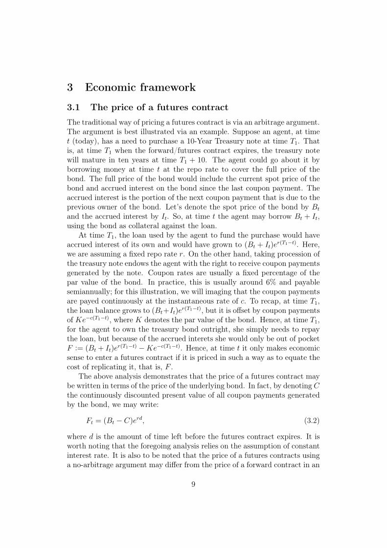
The traditional way of pricing a futures contract is via an arbitrage argument.The argument is best illustrated via an example. Suppose an agent, at timet (today), has a need to purchase a 10-Year Treasury note at time T1. Thatis, at time T1 when the forward/futures contract expires, the treasury notewill mature in ten years at time T1 + 10. The agent could go about it byborrowing money at time t at the repo rate to cover the full price of thebond. The full price of the bond would include the current spot price of thebond and accrued interest on the bond since the last coupon payment. Theaccrued interest is the portion of the next coupon payment that is due to theprevious owner of the bond. Let’s denote the spot price of the bond by Bt

and the accrued interest by It. So, at time t the agent may borrow Bt + It,using the bond as collateral against the loan.

At time T1, the loan used by the agent to fund the purchase would haveaccrued interest of its own and would have grown to (Bt + It)e

r(T1−t). Here,we are assuming a fixed repo rate r. On the other hand, taking procession ofthe treasury note endows the agent with the right to receive coupon paymentsgenerated by the note. Coupon rates are usually a fixed percentage of thepar value of the bond. In practice, this is usually around 6% and payablesemiannually; for this illustration, we will imaging that the coupon paymentsare payed continuously at the instantaneous rate of c. To recap, at time T1,the loan balance grows to (Bt+It)e

r(T1−t), but it is offset by coupon paymentsof Ke−c(T1−t), where K denotes the par value of the bond. Hence, at time T1,for the agent to own the treasury bond outright, she simply needs to repaythe loan, but because of the accrued interets she would only be out of pocketF := (Bt + It)e

r(T1−t) −Ke−c(T1−t). Hence, at time t it only makes economicsense to enter a futures contract if it is priced in such a way as to equate thecost of replicating it, that is, F .

The above analysis demonstrates that the price of a futures contract maybe written in terms of the price of the underlying bond. In fact, by denoting Cthe continuously discounted present value of all coupon payments generatedby the bond, we may write:

Ft = (Bt − C)erd, (3.2)

where d is the amount of time left before the futures contract expires. It isworth noting that the foregoing analysis relies on the assumption of constantinterest rate. It is also to be noted that the price of a futures contracts usinga no-arbitrage argument may differ from the price of a forward contract in an

9

environment with stochastic time varying interest rates. We refer the readerto Cox et al. (1981) for a lucid discussion of this point. For the intuitionwe wish to develop, the assumption of a constant in time interest rate istolerable.

Returning to (3.2), and taking the natural logarithm of both sides of theequation, and assuming that the face value of the bond is much larger thanthe present value of future coupon payments, we may write

ft ≈ bt − c+ rd, (3.3)

where bt := log(Bt) and c := log(C). Note that bt = −Tyt, where yt is theyield to maturity at time t of the bond. The quantity rd−c is usually referredto variously in the empirical literature as the carry or the basis. Looking atactual price data, the carry would fluctuate from time to time usually arounda long term mean. The basic idea of a mean-reverting carry is the motivationbehind the so-called carry-trade, which is implemented by going short thefutures and long the bond when the carry is high and doing the oppositewhen the carry is deemed too low. The strategy reviewed subsequently, isonly related to this trade by the fact that it relies on mean-reversion to beprofitable.

Returning to (3.3) it is apparent that besides the variation in the carry,variations in the logarithm of the futures price comes about because of vari-ations in the logarithm of the bond price, which is itself driven by the yieldto maturity of the bond. Usually, the carry does not vary by a whole lot andit is often modeled as a constant as we have done here unless, of course, theobject of the analysis is to study the carry itself. Given these considerationswe may model the logarithm of the price of the futures contract directly andexclusively in terms of the yield to maturity with no significant loss in rigor.That is, we may write

ft = α + βyt, (3.4)

where α and β are constant terms and yt is the yield to maturity of theunderlying bond. The constant α is simply the carry and whatever needsto be added or subtracted in order to make the approximation in (3.3) anequality. The constant β is in this setting equal to −T , that is, negative thetenor of the underlying bond.

The preceding reformulation of the logarithm of the price of a futurescontract in terms of the yield to maturity of the underlying bond allows usto use the theoretical machinery developed to study the term structure ofinterest rates to motivate the trading system that we discuss subsequently.

10

3.2 Factor model of the yield curve

Factor modeling of the yield curve has a rich history in the financial lit-erature. The extant models may be broadly classified under three mainheadings: statistical, no-arbitrage, and hybrid models. The static Nelson &Siegel (1987) (NS) model of the yield curve and its modern counterpart, theDynamic Nelson-Siegel (DNS) model, proposed by Diebold & Li (2006) areprototypes of the class of statistical factor models of the interest rate termstructure. They, especially the static Nelson & Siegel, are widely used bothby financial market practitioners and central banks to set interest rates andforecast yields. Despite their popularity and appealing statistical properties,they tend to give rise to violations of the no-arbitrage condition2.

The dynamic term structure models (DTSM) studied in (Singleton, 2006,Chapter12), of which the yield-factor model of Duffie & Kan (1996) is anearly example, constitute the class of arbitrage-free models. These modelsderive a functional form of the yield curve in terms of state variables orfactors, which also govern the market price of risk linking the local martin-gale measure to the historical measure. They are, therefore, by constructionarbitrage-free. Despite their economic soundness, these models tend to havesub-par empirical performance. For instance, Dybvig et al. (1996) showed inthe discrete-time setting that in an arbitrage-free model, long forward andzero-coupon rates can never fall; working in the general setting of continu-ous trading, Hubalek et al. (2002) arrived at a similar conclusion regardingthe monotonicity of long forward rates under the no-arbitrage assumption.Clearly, this implication of the no-arbitrage framework is often contradictedby the empirical evidence that zero-coupon rates do in fact fall. Furthermore,negative rates and unit roots are ruled out. As (Diebold & Rudebusch, 2013,p. 13) put it

Economic [no-arbitrage] theory strongly suggests that nominalbond yields should not have unit roots, because the yields arebounded below by zero, whereas unit root processes have randomwalk components and therefore will eventually cross zero almostsurely.

Negative interest rates post 2008 financial crisis are a mainstay of manydeveloped economies, including Switzerland. Moreover, the task of fittingarbitrage-free models to interest rate data can be very difficult since they tendto be over-parametrized and, typically, would generate multiple likelihoodmaxima (Diebold & Rudebusch, 2013, p. 55).

2See (Filipović, 1999) for such violations in the case of DNS models.

11

Lastly, the Arbitrage-Free Nelson-Siegel (AFNS) model proposed by Chris-tensen et al. (2011) is a prototype of the hybrid class of models. It main-tains the parsimonious parametrization of the DNS model while remainingarbitrage-free. The AFNS differs, at least in the functional form of the yieldcurve, from the standard DNS model only by the inclusion of an extra termknown as the “yield adjustment factor”. Intuitively, the AFNS model maybe thought of as the projection of an arbitrage-free affine term structuremodel, namely the Duffie & Kan (1996) model, onto the DNS model withthe orthogonal component swept into the yield adjustment factor.

The factor models briefly surveyed above motivate the trading rule adoptedin this paper; it relies on the hypothesis that the term structure of interestrates can be described by an affine function of a set of state variables, no-tably the level, slope, and curvature principal components. Moreover, thereis ample empirical evidence suggesting that the term structure is cointe-grated. In particular, using monthly Treasury bill data from January 1970until December 1988, Hall et al. (1992) observed that yields to maturity ofTreasury bills are cointegrated and that during periods when the FederalReserve specifically targeted short-term interest rates, the spreads betweenyields of different maturities defined the cointegrating vector.

In general, given a N ∈ N bonds, with N not necessarily finite, a factorsmodel of the yield curve would represent the yield on the i-th bond as:

yi,t = αt +

q∑j=1

βi,jfj,t + εi,t, (3.5)

where α is deterministic, q is a small number, fj for j = 1, · · · , q, are fac-tors βi,j is the contribution of the jth factor to the ith bond, and εi is thecomponent of the ith bond that is apart from any other bond. For our pur-poses, it does not actually matter whether the factors are macroeconomic orstatistical in nature, but to fix ideas we assume q = 3 and the factors arethe level, slope, and curvature factors of Litterman & Scheinkman (1991).By substituting the expression in (3.5) into equation (3.4), we obtain the logfutures price in terms of the level, slope, and curvature of the term structure.That is,

fi,t = µt +3∑j=1

γi,jfj,t + εi,t.

3.3 Factor extraction

Using Principal Component Analysis (PCA), it is possible to transform theoriginal time series of futures prices into a set of orthogonal time series known

12

as principal components. Because of the orthogonality property, the origi-nal time series may be expressed uniquely as a linear combination of theprincipal components. This representation motivates the interpretation ofthe principal components as the latent risk factors driving observed pricefluctuations.

The analysis starts with n observations from an m-dimensional randomvector, the original time series data. Then, assuming that the original timeseries admits a stationary distribution with finite first and second moments,the covariance matrix is estimated using an unbiased and consistent estima-tor. In our setting, the assumption of stationarity applied directly to thelogarithm of futures prices is hard to justify. Prices generally trend upward,and the same may be expected for their log-transformed versions. Usingthe Augmented Dickey-Fuller (ADF) statistics with constant drift, we testthe hypothesis that the lag polynomial characterizing the underlying datagenerating process has a unit root.

A quick scan of Table 1 reveals that for the most part the unit root as-sumption cannot be rejected. The only exception seems to be the 2 Year andthe 5 Year futures price data for the year 2015, for which the assumption ofa unit root may be rejected at the 5% confidence level. We think this out-come is a temporary fluke since for the previous five years the null hypothesiscould not be rejected. We have also looked at different subsamples of the2015 data, and for the most part the assumption of a unit root could not berejected.

Under the circumstances, carrying on with the analysis of the principalcomponents of the original price series may not be advisable. Without thestationarity assumptions, it is very likely the case that the usual estimatorof the covariance matrix would yields estimates that may be substantiallyoff the mark. Meanwhile, taking the first difference of the logarithm of theprice series seems to produce time series that display very little persistenceas may be observed from an inspection of Figure 1. Hence, the assumptionof stationarity may be more appropriate only after differencing the data. Wehave substantiated this assumption using the ADF test and the unit rootassumption was rejected at the 1% confidence level.

Clearly, taking differences of the log price data entails a loss of informa-tion. Nevertheless, an analysis of the differenced data could still yield insightinto the factor structure of the original price data since the property couldbe expected to be shared by both the differenced data and the data in levels.This observation is easily confirmed by means of simple algebraic manipula-tions. Naturally, the factors that may be extracted from the differenced datawould bear very little resemblance to the factors present in the levels data,so that there are limits to how much can be inferred about the data in levels

13

Table 1: Augmented Dickey-Fuller Tests

(a) 2010a t(a) lag t(lag) 5% c.value(a) 5% c.value(lag)

2 Yr 0.00 2.17 -0.00 -2.16 4.59 -2.865 Yr 0.00 2.01 -0.00 -2.00 4.59 -2.8610 Yr 0.00 2.05 -0.00 -2.05 4.59 -2.8630 Yr 0.00 2.03 -0.00 -2.02 4.59 -2.86

(b) 2011a t(a) lag t(lag) 5% c.value(a) 5% c.value(lag)

2 Yr 0.00 0.96 -0.00 -0.96 4.59 -2.865 Yr 0.00 0.62 -0.00 -0.61 4.59 -2.8610 Yr 0.00 0.56 -0.00 -0.54 4.59 -2.8630 Yr 0.00 0.36 -0.00 -0.33 4.59 -2.86

(c) 2012a t(a) lag t(lag) 5% c.value(a) 5% c.value(lag)

2 Yr 0.01 2.51 -0.00 -2.51 4.59 -2.865 Yr 0.00 1.31 -0.00 -1.31 4.59 -2.8610 Yr 0.00 1.22 -0.00 -1.21 4.59 -2.8630 Yr 0.00 1.36 -0.00 -1.36 4.59 -2.86

(d) 2013a t(a) lag t(lag) 5% c.value(a) 5% c.value(lag)

2 Yr 0.00 1.45 -0.00 -1.45 4.59 -2.865 Yr 0.01 1.85 -0.00 -1.85 4.59 -2.8610 Yr 0.00 1.65 -0.00 -1.65 4.59 -2.8630 Yr 0.00 1.24 -0.00 -1.25 4.59 -2.86

(e) 2014a t(a) lag t(lag) 5% c.value(a) 5% c.value(lag)

2 Yr 0.00 1.06 -0.00 -1.05 4.59 -2.865 Yr 0.00 1.46 -0.00 -1.46 4.59 -2.8610 Yr 0.00 1.74 -0.00 -1.73 4.59 -2.8630 Yr 0.00 1.95 -0.00 -1.93 4.59 -2.86

(f) 2015a t(a) lag t(lag) 5% c.value(a) 5% c.value(lag)

2 Yr 0.01 2.88 -0.00 -2.88 4.59 -2.865 Yr 0.01 3.01 -0.00 -3.01 4.59 -2.8610 Yr 0.01 2.76 -0.00 -2.76 4.59 -2.8630 Yr 0.00 1.65 -0.00 -1.65 4.59 -2.86

14

Figure 1: Changes in log prices

(a) 2 Yr Treasury Note (b) 5 Yr Treasury Note

(c) 10 Yr Treasury Bond (d) 30 Yr Treasury Bond

15

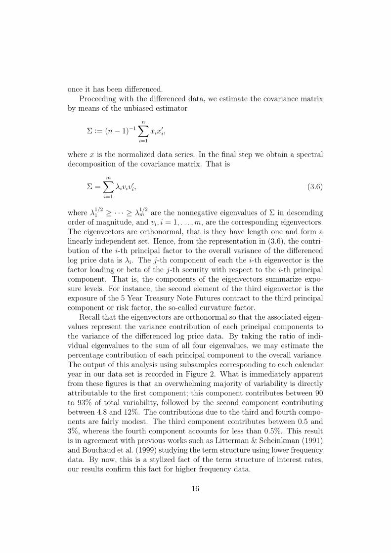
once it has been differenced.Proceeding with the differenced data, we estimate the covariance matrix

by means of the unbiased estimator

Σ := (n− 1)−1n∑i=1

xix′i,

where x is the normalized data series. In the final step we obtain a spectraldecomposition of the covariance matrix. That is

Σ =m∑i=1

λiviv′i, (3.6)

where λ1/21 ≥ · · · ≥ λ1/2m are the nonnegative eigenvalues of Σ in descending

order of magnitude, and vi, i = 1, . . . ,m, are the corresponding eigenvectors.The eigenvectors are orthonormal, that is they have length one and form alinearly independent set. Hence, from the representation in (3.6), the contri-bution of the i-th principal factor to the overall variance of the differencedlog price data is λi. The j-th component of each the i-th eigenvector is thefactor loading or beta of the j-th security with respect to the i-th principalcomponent. That is, the components of the eigenvectors summarize expo-sure levels. For instance, the second element of the third eigenvector is theexposure of the 5 Year Treasury Note Futures contract to the third principalcomponent or risk factor, the so-called curvature factor.

Recall that the eigenvectors are orthonormal so that the associated eigen-values represent the variance contribution of each principal components tothe variance of the differenced log price data. By taking the ratio of indi-vidual eigenvalues to the sum of all four eigenvalues, we may estimate thepercentage contribution of each principal component to the overall variance.The output of this analysis using subsamples corresponding to each calendaryear in our data set is recorded in Figure 2. What is immediately apparentfrom these figures is that an overwhelming majority of variability is directlyattributable to the first component; this component contributes between 90to 93% of total variability, followed by the second component contributingbetween 4.8 and 12%. The contributions due to the third and fourth compo-nents are fairly modest. The third component contributes between 0.5 and3%, whereas the fourth component accounts for less than 0.5%. This resultis in agreement with previous works such as Litterman & Scheinkman (1991)and Bouchaud et al. (1999) studying the term structure using lower frequencydata. By now, this is a stylized fact of the term structure of interest rates,our results confirm this fact for higher frequency data.

16

Figure 2: Variance contributions

(a) 2010 (b) 2011

(c) 2012 (d) 2013

(e) 2014 (f) 2015

17

Figure 3: Factor loadings by contract

(a) 2010 (b) 2011

(c) 2012 (d) 2013

(e) 2014 (f) 2015

18

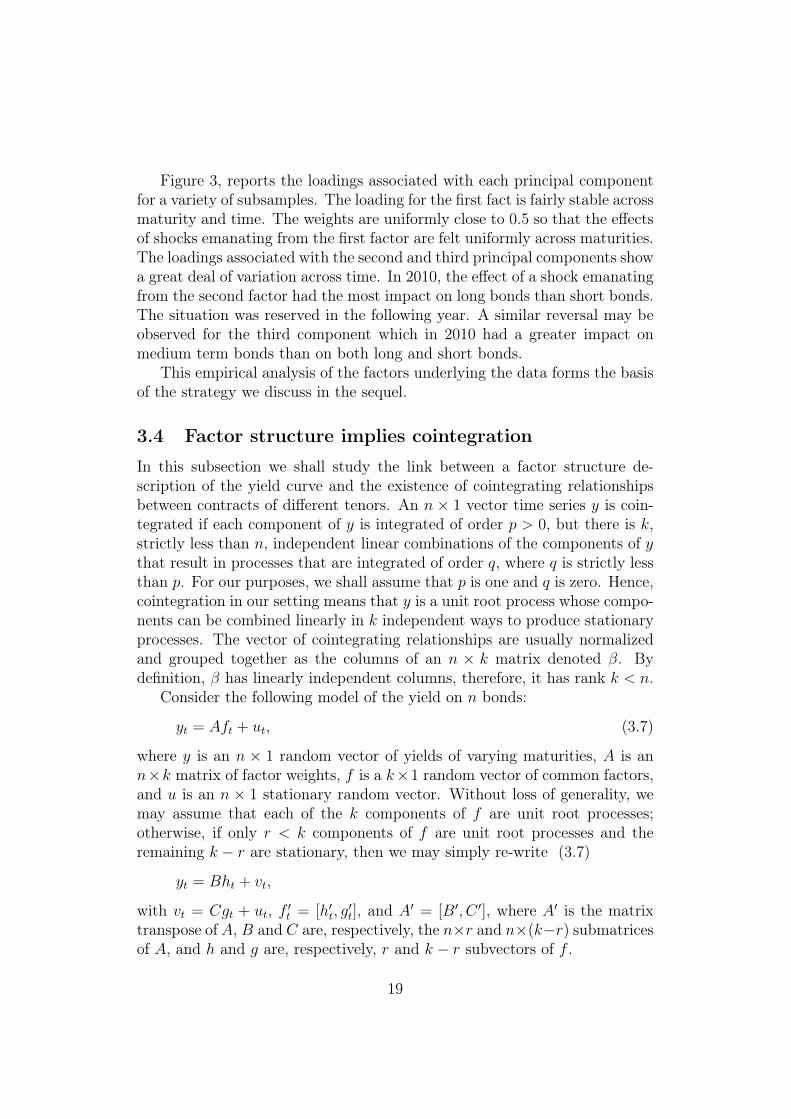
Figure 3, reports the loadings associated with each principal componentfor a variety of subsamples. The loading for the first fact is fairly stable acrossmaturity and time. The weights are uniformly close to 0.5 so that the effectsof shocks emanating from the first factor are felt uniformly across maturities.The loadings associated with the second and third principal components showa great deal of variation across time. In 2010, the effect of a shock emanatingfrom the second factor had the most impact on long bonds than short bonds.The situation was reserved in the following year. A similar reversal may beobserved for the third component which in 2010 had a greater impact onmedium term bonds than on both long and short bonds.

This empirical analysis of the factors underlying the data forms the basisof the strategy we discuss in the sequel.

3.4 Factor structure implies cointegration

In this subsection we shall study the link between a factor structure de-scription of the yield curve and the existence of cointegrating relationshipsbetween contracts of different tenors. An n × 1 vector time series y is coin-tegrated if each component of y is integrated of order p > 0, but there is k,strictly less than n, independent linear combinations of the components of ythat result in processes that are integrated of order q, where q is strictly lessthan p. For our purposes, we shall assume that p is one and q is zero. Hence,cointegration in our setting means that y is a unit root process whose compo-nents can be combined linearly in k independent ways to produce stationaryprocesses. The vector of cointegrating relationships are usually normalizedand grouped together as the columns of an n × k matrix denoted β. Bydefinition, β has linearly independent columns, therefore, it has rank k < n.

Consider the following model of the yield on n bonds:

yt = Aft + ut, (3.7)

where y is an n × 1 random vector of yields of varying maturities, A is ann×k matrix of factor weights, f is a k×1 random vector of common factors,and u is an n × 1 stationary random vector. Without loss of generality, wemay assume that each of the k components of f are unit root processes;otherwise, if only r < k components of f are unit root processes and theremaining k − r are stationary, then we may simply re-write (3.7)

yt = Bht + vt,

with vt = Cgt + ut, f ′t = [h′t, g′t], and A′ = [B′, C ′], where A′ is the matrix

transpose of A, B and C are, respectively, the n×r and n×(k−r) submatricesof A, and h and g are, respectively, r and k − r subvectors of f .

19

Returning to equation (3.7), the vector of factors may be assumed to bea multivariate random walk, i.e.,

ft = ft−1 + φ(L)εt,

where φ(L) is a lag polynomial, ε is white noise, and φ(L)ε is stationary.There some empirical evidence in our data that this assumption is not un-justifiable. Using a matrix analysis argument, details of which may be foundin Theorem 3.1 of Escribano & Pena (1993), it is easy to verify that y maybe written as a sum of a stationary process and a unit root process:

yt = wt + zt,

where w ∼ I(1) and z ∼ I(0). Both w and z may be computed explic-itly given the matrix of factor loadings as follows: wt = AA′yt and zt =(A⊥)′A⊥yt, where A⊥ is the orthogonal complement of A, i.e. (A⊥)′A = 0.Now, setting β := (A⊥)′, it is easily seen that βyt = βzt ∼ I(0), so that β isa matrix of cointegrating vectors. Hence, cointegration of the vector of yieldsis a consequence of the factor structure of the yield curve.

The analysis in the previous section provides some indirect empirical sup-port for the existence of orthogonal risk factors underlying the dynamics ofthe term structure. Recall that our analysis of the factors employed differ-enced price data. So, direct measurements of the risk factors is not an option,but we could at least extract the differenced factors and compute their cu-mulative sum. While this approach may lack rigor, it nevertheless provides aglimpse of what the original factors might look like. Using the reconstructedrisk factors, we test the hypothesis that the level, slope, and curvature factorsare unit root processes. The result of this analysis is recorded in Table 2.The results show that the hypothesis of unit root for the risk factors may notbe reject at any reasonable level for any of the six calendar years included inour data set.

3.5 Cointegration implies a factor structure

In the previous section, we argued that cointegration is natural assuming theunderlying data admits a factor structure. In this section, we argue that theconverse is also true. Starting with the assumption that the components ofy are integrated of order one, y may be expressed, using lag polynomials, as:

(1− L)yt = Φ(L)εt, (3.8)

where ε is n × 1 iid noise, L is the lag operator, Φ(L) =∑∞

j=1 ΦjLj, Φj is

n× n matrix, and Φ0 is the n× n identity matrix. The last condition is anaccommodation for the presence of a deterministic linear trend.

20

Cointegration entails a restriction of the process Φ(L)ε, and on Φ(1) inparticular. Indeed, writing Φ(L) = Φ(1) + (1 − L)Φ∗(L), where Φ∗(L) :=(1− L)−1(Φ(L)− Φ(1)), equation (3.8) may be expressed as:

(1− L)yt = Φ(1)εt + (1− L)Φ∗(L)εt. (3.9)

Solving (3.9) by recursive substitution yields

yt = Φ(1)zt + Φ∗(L)εt, (3.10)

where zt :=∑t−1

i=0 εt−i. Now, cointegration implies the existence of an n× kmatrix β, the matrix of cointegrating vectors, such that β′yt is integrated oforder 0; but since zt is a multivariate random walk, it must be the case thatβ′Φ(1) = 0. Now, since β has rank r and Φ spans the subspace orthogonalto its column space, it must be the case that Φ(1) has rank n− k.

Using the Jordan canonical form, we may write

Φ(1) = AJA−1

where J is a (n − k) × (n − k) diagonal matrix containing the non-zeroeigenvalues of Φ(1), A the corresponding n× (n− k) matrix of eigenvectors,and A−1 is the right inverse of A. This decomposition is possible because Φonly has n − 1 non-zero eigenvalues. Now setting ut := JA−1εt and νt :=Φ∗(L)εt, and substituting into (3.10) yields

yt = Aft + νt, (3.11)

where ft = ft−1 + ut. The interesting thing about (3.11) is that f is an(n − k) × 1 unit root process driving y. That is cointegration implies afactor structure. This result appears at various levels of generality in Stock& Watson (1988) and Escribano & Pena (1993).

4 MethodologyThe basic trading mechanism consists of two main steps. The first step testsfor cointegration between the four futures prices and estimates the paramtersof a stationary portfolio of the four contracts under the hypothesis of cointe-grated prices. The portfolio weights are the components of the cointegrationvector. We use a month’s worth of daytime (7:30 to 14:00 CT) trading datasampled at one minute intervals for this step. This period is the so-called for-mation period. Besides estimating the cointegration vector, we also estimatethe first two central moments of the stationary portfolio.

21

Table 2: Augmented Dickey-Fuller Tests

(a) 2010Level Slope Curvature

intercept 0.00 0.00 0.00t-stat (intercept) 2.32 2.10 1.87

lag -0.00 -0.00 -0.00t-stat(lag) -2.08 -1.97 -1.88

(b) 2011Level Slope Curvature

intercept 0.00 -0.00 -0.00t-stat (intercept) 1.78 -1.74 -1.52

lag -0.00 -0.00 -0.00t-stat(lag) -0.46 -0.31 -0.24

(c) 2012Level Slope Curvature

intercept 0.00 0.00 0.00t-stat (intercept) 1.01 1.04 0.85

lag -0.00 -0.00 -0.00t-stat(lag) -1.30 -1.30 -1.50

(d) 2013Level Slope Curvature

intercept -0.00 -0.00 -0.00t-stat (intercept) -1.26 -1.34 -1.33

lag -0.00 -0.00 -0.00t-stat(lag) -1.51 -1.21 -0.79

(e) 2014Level Slope Curvature

intercept 0.00 0.00 -0.00t-stat (intercept) 2.34 2.62 -2.71

lag -0.00 -0.00 -0.00t-stat(lag) -1.75 -2.03 -2.31

(f) 2015Level Slope Curvature

intercept 0.00 0.00 0.00t-stat (intercept) 1.89 0.34 1.37

lag -0.00 -0.00 -0.00t-stat(lag) -2.27 -1.56 -1.42

22

In the second step, we start monitoring prices immediately after the for-mation period to identify price configurations that may be too rich or toocheap according to our estimates of the first two moments from the forma-tion period. This so-called trading period lasts for about three weeks (100daytime trading hours) from the end of the formation period. Specifically,we consider the price configuration to present a buy opportunity, if the priceof the stationary portfolio falls below two standard deviations of the sam-ple mean computed on the basis of the data generated during the formationperiod. There is a sell opportuitity if the price climbs beyond two standarddeviations of the mean price from the formation period. Hence, a position isentered into whenever the price of the synthetic asset, constructed from thecointegration vector, veers outside the two standard deviation band; the po-sition is long or short according to whether the price configuration is deemedcheap or rich. Short-sale constraints are almost non-existent in the futuresmarket, so they do not enter into our analysis.

Position are opened at any time during the trading period; they are closedas soon as the price of the synthetic asset experiences a large enough cor-rection after its excursion away from the sample mean estimated from theformation period. Specifically, a position is closed as soon as the price fallswithin the one standard deviation band. Hence, after each correction, atleast one standard deviation is earned on the round-trip trade. This processis continued until the end of the trading period at which time all open po-sitions are liquidated at the quoted price. Generally, this is the only time aloss can be registered, since a correction might not have taken place prior tothe end of the trading period.

The entire process is repeated on a rolling window from the start of thesample (1 April 2010) to the end of the sample (31 December 2015). Inboth steps we use exclusively quote data as opposed to transaction data. Anadvantage of using quote data is that the data is simply more plentiful andmay better accurately represent the state of the market as perceived by anagent at any given moment. During the synthetic portfolio formation stage,the cointegration vectors and the first two moments are estimated using themidpoint of the best bid and ask prices. During the trading stage, positionsare opened and closed using quoted bid and ask prices: a long position isentered into at the ask and shorts executed at the bid.

The evaluation of the strategy using quotes prices is imperative given theshort-term nature of the strategy. All positions are opened for at most 100daytime trading hours. Theoretically, a position could be entered into andexited the very next minute. For such short investment horizons, the bid-askspread looms very large. By using quote data, execution costs arising fromthe bid-ask spread is automatically taken into account. Of course, there are

23

other types of execution costs, but the bid-ask spread is usually the largestsource of execution costs, and the use of quoted prices takes care of it rightaway.

5 Results

5.1 Return calculation

Evaluating the performance of a trading strategy that may involve long andshort positions is not altogether a straight foreword matter. In fact, theliterature gives little guidance on how to define the one-period return of aportfolio consisting of long and short positions. The issue is without com-plications for a portfolio consisting entirely of long positions; the one-periodreturn is simply the difference between the starting and ending value of theportfolio divided by its starting value. Unfortunately, this definition presentsdifficulties as soon as portfolios with both long and short positions are con-sidered. For such portfolios, the initial investment could be arbitrarily small,zero, or even negative due to the offsetting effects of long and short posi-tions. In the case of a zero-cost portfolio, the period return is ether positiveinfinity or negative infinity, regardless of the actual change in the value ofthe portfolio.

It is easy to see that the standard definition is problematic for portfolioswith both long and short positions because the value of the portfolio at thestart of the period is always taken as the basis for measuring the performanceof the portfolio over the period. By reconsidering the investment simply interms of cash inflows and outflows much of the difficulties of the standardapproach may be overcome. The cash flow perspective, assumes that theentire portfolio is marked to market at the end of each investment period, sothat there is a cash flow at the start and end of each period. Cash inflowsand outflows are defined from the perspective of the investor. A long positioninvolves an initial cash outflow followed by a cash inflow at the end of theperiod. The situation is reversed for short positions: an initial cash inflowfollowed by a cash outflow at the end of the period. Given a portfolio of longand short positions, the one period return is simply the natural logarithmof the ratio of the total cash inflows, from both types of positions, to thetotal cash outflows, also from both long and short positions. This measure isapproximately equal to the ratio of the difference between cash inflows andoutflows to cash outflows for the period. That is

rt = log

(InflowstOutflowst

)≈ Inflowst −Outflowst

Outflowst. (5.12)

24

While this definition of period return may seem reasonable for perfor-mance measurement in the majority of spot/cash markets, it is not withoutcontroversy where futures markets are concerned. Black (1976) observed thatit is, in principle, impossible to define fractional or percentage returns for aposition in futures contracts. This is because, the time t quoted price of afutures contract is merely the price at which the underlying instrument maybe exchanged at an agreed upon future date; no actual transactions occurimmediately, so that there are no cash outlays at time t. There is only onetransaction, and it occurs at the end of the contract in the form of an out-flow or inflow but not both. In practice, both the long and the short sidesof a futures contract are required by the trading venue to post collateral tooffset the risk of default. Ordinarily, there is a mandated minimum collateralrequired by the brokerage firm used by the investor. This minimal collateralis otherwise known as the initial margin.

A position in futures contracts is marked to market daily, so that favor-able price moves results in credits and unfavorable price moves as debits tothe margin account. To prevent the margin account from being entirely de-pleted in the event of a succession of unfavorable price moves, the exchangemay set a maintenance margin, which is a minimum balance that must bemaintained in the margin account at all times after the initial transaction.Usually, the maintenance margin is the same amount as the initial margin,but it may sometime lower. Margin requirements may differ according towhether the investor is classified as a member of the exchange or a non-member speculator. In 2016, the margin requirements for investors withoutmembership licenses to the Chicago Mercantile Exchange(CME) is 10% morethan the margin requirement for members of the CME.

Technically, the margin is not to be taken as an initial investment, but itmay be argued that it is the amount of cash required to make the transactionpossible; without it, the position can not be established. Arguing in thismanner, we may define the return of a long position in a futures contractat time t to be the change in the price of the contract divided by the initialmargin. That is

rt =Ft − Ft−1

M, (5.13)

where M is the initial margin and Ft is the price at the end of time t ofthe futures contract. For a short position, the numerator above is multipliedby negative one. This basic definition is also plagued by the usual problemsencountered when computing the return generated by a portfolio of bothlong and short positions. Reasoning as in (5.12), the return metric definedin (5.13) based on the timing of cash flows may be modified to only take

25

into account the direction of cash flows. Hence, given n different futurescontracts, we may define the performance metric

rt =

∑ni (Inflowsi,t −Outflowi,t)∑

i Leverage Ratioi,t × Par Valuei,t ×Qi,t

. (5.14)

where the leverage ratio is simply the ratio of the initial margin of the i-thcontract to the par value of the underlying bond, and Qi,t is the exposure, interms of number of contracts, to the i-th contract at time t. In our setting nis four and the contracts are distinguished by their tenors. Definition (5.12)is a special case of the above; it holds when the position is fully founded,that is, when the leverage ratio is one.

Table 3: Time-averaged CME margin requirements between 1 April 2010 and 12December 2015.

Initial marginContracts Notional value Members Speculators

2 Yr 200000 448 4935 Yr 100000 818 90010 Yr 100000 1323 145630 Yr 100000 2647 2912

The initial margins are ordinarily not the same across contracts and,therefore, must be handled carefully. For instance, in the last quarter of 2016,the initial margin for the 30-Year Treasury Bond Futures contract was $4000,whereas the initial margin of the 2-Year Treasury Note Futures contract wasonly $550. Beside the differences in initial margins by contract types, thereare also variations over time. For most of 2010, the initial margin requirementfor the 5-Year Treasury Note Futures contract was $800 for investors withmembership licenses and $880 for non-members. Meanwhile, for all of 2014,the initial margin for the same contract was $900. To simplify our analysis,we compute a time-weighted average of the initial margin for the time periodbetween 1 April 2010 and 31 December 2015 for each contract type. The timeweighted average for members and non-members of the CME are recorded inTable 3. As may be expected, margin requirements increase with the tenorof the underlying, because the price of contracts with longer maturities aremore likely to experience large price swings.

As previously stated, the initial margin is merely the minimum collateralrequired to initiate a transaction in one futures contract. An investor maychose to apply however much collateral he or she desires. If each transaction

26

is fully funded, i.e., if the exact amount of the exposure to each contractis always set aside for each transaction, then the appropriate performancemeasure would be a slight modification of the formula given in (5.12). Thatis

rt =

∑ni (Inflowsi,t −Outflowi,t)∑

iOutflowi,t

. (5.15)

We remark that the use of fully funded accounts in the treasury futuresmarket is not very common. Consider that the notional value of the 2-Yeartreasury futures contract is $200,000 and $100,000 for the others. Hence,putting together a portfolio consisting of even a small number of contractsquickly becomes prohibitively capital intensive. Meanwhile, treasury futures,even those written on long bonds, have relatively stable long-term prices. Asa result, investments in the treasury futures market are most often under-taken using leverage or a margin account.

We conclude this section with a remark on the distinction between aninvestment period and a trading period. Trading periods are fixed: they areexactly 6000 daytime trading minutes, approximately 14 trading days. Aninvestment period is simply the time between when a position is opened andthe time when it is closed. Positions are opened when the price configurationsof the four securities indicate a departure from the stable relationship estab-lished during the preceding formation period. The positions are closed whenthe stable relationship is restored. This deviation and restoration towards astable relationship may occur several times during a single trading period,thereby creating multiple opportunities and, hence, investment periods.

The return formulas in (5.14) and (5.15) relate to the return over a singleinvestment period. For trading periods with multiple periods, we computethe return over the trading period as the sum of the individual returns gener-ated from each investment period contained within the trading period. Thatis

rt =

q∑i=1

ri,t

where ri,t is the return, computed via formula (5.14) or (5.15), of the i-thinvestment period of the t-th trading period, and q is the total number ofinvestment periods occurring in the t-th trading period.

5.2 Excess returns

We summarize the distribution of returns generated by backtesting the coin-tegration strategy described in the previous section in Table 4. The backtest

27

Table 4: Annualized (100 trading hours) returns on initial margin and fully fundedaccount.

Panel A: Fully-funded excess return over the equal-weighted portfolio

Ratio Difference

Average return 0.0604 0.05995Standard error (Newey-West) 0.02625 0.02737t-Statistic 2.3012 2.18984Excess return distribution

Median 0.04749 0.03655Standard deviation 0.30453 0.35263Skewness 2.12072 1.66976Kurtosis 14.58188 9.49711Minimum -0.68255 -0.752265% Quantile -0.29139 -0.3523495% Quantile 0.51928 0.61858Maximum 1.85812 1.79468% of negative excess returns 40.625 44.79167

Panel B: Return on margin account

Ratio Difference

Average return 15.12327 14.95951Standard error (Newey-West) 3.87113 4.13448t-Statistic 3.90668 3.61823Excess return distribution

Median 0.6238 0Standard deviation 46.01987 51.17213Skewness 1.63053 1.29959Kurtosis 10.99074 7.87337Minimum -105.68033 -110.641475% Quantile -51.1802 -70.3208695% Quantile 83.25456 96.94193Maximum 259.66658 250.56902% of negative excess returns 14.58333 16.66667

28

is run over daytime trading hours between April 1, 2010 and December 31,2015. The entire period is divided into 96 hundred-hour trading periodslasting approximately three business weeks. The figures shown in the tableare the annualized hundred-hour returns. We show cash flow-based returnscomputed on a fully funded account in the first panel of the table; the secondpanel displays the distribution of cash flows-based returns computed usingthe initial margin as the cost basis. Each panel reports two sets of backtestresults: one for prices adjusted backwards by the application of a propor-tional factor (Ratio) and the other for prices shifted in levels backward bythe amount of the roll-induced price gap (Difference).

Now, the annualized excess return over the equally weighted portfolioof all four contracts, assuming a fully-funded account, are 6.01% and 6.00%respectively for the ratio and the difference price adjustment procedures. TheNewey-West adjusted t statistics are 2.3 and 2.2, respectively. Given thisresult, the hypothesis that the cointegration strategy dominates the equal-weighted portfolio, cannot be rejected. The idea is that one may short asmany of the equal-weighted portfolio as necessary and use the proceeds toset up the cointegration strategy without incurring a loss.

Meanwhile, the annualized return using the initial margin as the cost basisare, respectively, 1500% and 1490%. These returns are not as preposterous asthey first seem. Consider that the leverage factor implicit in the initial marginfor the 2-Year contract is 446 and that of the 5-Year contract is 122. Theinflated returns are, therefore, merely a consequence of the inflated leveragefactors. The t statistics in both cases are in excess of 2. Also, note thatthe out-sized returns that may be achieved by trading on the initial margincome at the expense of taking significant risks: consider that the standarddeviation of the returns on initial margin are 159.17 times the volatility of thereturn on the fully funded account. Clearly, in practice, what an investor endsup doing would be somewhere between trading a fully-funded account andposting the minimum required collateral. At any rate, our analysis providesa starting point for reasoning about how to incorporate leverage in a morerealistic real world strategy.

5.3 Statistical Arbitrage

Stephen Ross (1976) gave the first serious treatment of the concept of arbi-trage. While his treatment might have been of a heuristic nature, it never-theless conveyed the essence of an arbitrage, which is a trading strategy thatyields a positive payoff with little to no downside risk. The first rigorousdefinition appeared in Huberman (1982), where it was defined in the contextof an economy with asset generated by a set of risk factors as a sequence of

29

portfolios with payoffs φn such that E(φn) tends to +∞ while Var(φn) tendsto 0. The concept has undergone numerous changes in the literature, see forexample Kabanov (1996), but the essential meaning of the term as a low riskrisk investment still remains. We focus on a special type of arbitrage knownin the empirical asset pricing literature as a statistical arbitrage, which Hoganet al. (2004) defines as a zero-cost, self-financing strategy whose cumulativediscounted value v(t) satisfies:

1. v(0) = 0,

2. limt→∞E(vt) > 0,

3. limt→∞ P (vt < 0) = 0, and

4. if v(t) can become negative with positive probability, then Var(vt <0)/t→ 0 as t→∞.

Even though the above notion of arbitrage bears resemblance to the originaldefinition given by Huberman (1982), it is worth noting that there is a cru-cial difference between the two concepts. In the first instance, the limit istaken with respect to the cross-section of the economy, i.e. the sequence ofsmall economies is assumed to expand without bound, whereas the definitiongiven above requires the investment horizon to tend to infinity. It is easilyverified that the first three conditions, assuming the existence of the firstmoment correspond to the definition of an arbitrage in the classical senseof (Delbaen & Schachermayer, 1994). Chapter 2 of Dare (2017), obtains aseries of equivalent characterizations of market efficiency. In particular, Dare(2017, Proposition 2.1) shows that a necessary condition for market efficiencyis the existence of a local martingale measure after expressing asset pricesin units of any strictly positive convex portfolio of the zeroth asset and anyother asset (possibly itself). To apply this result, we express prices in unitsof the 2-Year treasury futures contract and attempt to exhibit a violation ofthe no-arbitrage condition.

Following Hogan et al. (2004) we propose to test market efficiency underthe assumption that the change in the discounted cumulative gains of thestrategy satisfies:

vt − vt−1 = µ+ σtλzt, (5.16)

where t is an integer; σ, λ, and µ are real numbers; and zt is an i.i.d. se-quence of standard normal random variables. The model allows for determin-istic time variation in the second moment, but makes the seemingly strongassumption that there is no serial correlation between returns. Our own

30

simulations reveal that the effects of serial correlations are slight. In fact,assuming z were generated by an AR(1), differences of more than 10% onaverage standard errors only start to occur for values of the autoregressiveparameter in excess of 0.9 in absolute value. Since, the sample autocorre-lation of the returns of the strategy is only -0.158, it is likely the case thatserial autocorrelation is a minor issue.

The inference strategy we have adopted is not without weaknesses. Astylized empirical fact of financial markets is that asset returns generally havefat-tail distributions. The normality assumption may therefore seem overlyrestrictive. Moreover, the adopted parametric model may itself be a source ofmisspecification errors. A more sophisticated analysis would perhaps employrobust tools such as the bootstrap.

While the above criticisms may be valid, note that the test statisticsdiscussed in Hogan et al. (2004) and Dare (2017, Chapter 2) are very con-servative because they rely on the Bonferroni criterion, which stipulates thatin compound tests involving a joint-hypothesis, the sum of the p-values ofthe individual tests is an upper limit for the Type I error of the compoundtest (Casella & Berger, 1990, p.11).

The test of efficiency then consists of estimating the parameters of (5.16)and then testing for

1. µ > 0, and

2. λ < 0.

For, under the null hypothesis, the cumulative returns will increase with-out bound as the variance of the cumulative gain tends to zero. Under theassumption of normally distributed zt, the test can be carried out by max-imum likelihood estimation. Table 5 summarizes the results of estimatingmodel (5.16). The p-value of the joint test using the Bonferonni correction,which consists of adding up the p-values from each sub-hypothesis, of thepresence of a statistical arbitrage is approximately 0.02 in both the ratio anddifference-adjusted price series.

Table 5: Test for statistical arbitrage

Difference RatioPar. Estimate Std Error p-value Estimate Std Error p-value

µ 0.3351 0.0108 <0.01 0.3735 0.0106 <0.01σ 1.151 0.5397 0.041 4.98 3.2077 0.1195λ -0.6808 0.1288 <0.01 -1.0353 0.1779 <0.01

31

The p-value for the estimates of σ are relatively large, estecially for theratio adjusted price series. This is to be extected since for large t, the volatil-ity of incremental payoffs is mostly determined by the term tλ and not σ.We conduct a separate test with σ restricted to 1. The output of that test isrecorded in Table 6. The estimates and p-value obtained from the restrictedmodel match the estimates from the unrestricted model. These results pro-vide a strong indication that the strategy not only earns positive excess returnover the equal weighted portfolios, but also, a positive free-lunch.

Table 6: Test for statistical arbitrage (σ = 1)

Difference RatioPar. Estimate Std Error p-value Estimate Std Error p-value

µ 0.333 0.0082 <0.01 0.3474 0.0104 <0.01λ -0.6452 0.0199 <0.01 -0.5885 0.0204 <0.01

6 ConclusionStarting with the assumption that interest rates and, therefore, bond futuresprices admit a factor structure, we evaluate a trading strategy based on theassumption of cointegrated bond futures prices. We argue that coitegration isnatural if in fact the dynamics of the yield curve is driven by orthogonal riskfactors which together form a jointly unit root process. Direct verificationof this hypothesis is difficult because the price series and its log transfomedcounterparts are likely not stationary. On the other, the stationary assump-tion can be made and tested using the change in log prices. Using differencedprice data, we argued empirically that the vast majority of the volatility ex-perienced by the changes in log prices may arise from three dominant riskfactors. Since the factors are othogonal and the differenced log prices maybe assumed to be stationary, there is very little doubt that the factors con-tained in the differenced log prices are stationary. To test the claim for thelog prices in evels, we estimated the factors in levels by taking cumulativesums of the factors estimated using differenced log prices. For these proxiesof the factors in levels, the assumption of unit roots could not be rejected atreasonable significant levels.

With the choice of cointegrating strategy properly motivated, we pro-ceeded to evaluate a simple trading strategy based on the cointegration hy-pothesis. The crust of the strategy consists in opening a position as soonthe price configuration appears to deviate from an estimated stable cointe-

32

gration relationship. The strategy is evaluated by computing the ratio ofcash-equivalent inflows to outflows. We also consider a return metric basedon the initial margin required to take either a short or a long position inone futures contract. Our results reveal that the gains from this strategyare both economically and statistically significant. This exercise allows toargue along the lines innitiated by Jarrow & Larsson (2012) that the U.S.treasury bond futures market, for the period for which we have data, wasnot informationally efficient.

33

ReferencesBlack, Fischer (1976) “The pricing of commodity contracts”, Journal of Fi-nancial Economics, Vol. 3, pp. 167–179.

Bouchaud, Jean-Philippe, Sagna, Nicolas, Cont, Rama, El-Karoui, Nicole,and Potters, Marc (1999) “Phenomenology of the interest rate curve”, Ap-plied Mathematical Finance, Vol. 6, pp. 209–232.

Bradley, Michael G. and Lumpkin, Stephen A. (1992) “The treasury yieldcurve as a cointegrated system”, The Journal of Financial and QuantitativeAnalysis, Vol. 27, No. 3, pp. 449–463.

Casella, George and Berger, Roger L. (1990) Statistical inference: ThomsonLearning, 2nd edition.

Christensen, J.H.E, Diebold, F.X., and Rudebusch, G.D (2011) “The affinearbitrage-free class of nelson-siegel term structure models”, Journal ofEconometrics, Vol. 164, pp. 4–20.

Cox, John C., Jonathan E. Ingersoll, Jr., and Ross, Stephen A. (1981) “Therelation between forward prices and futures prices”, Journal of FinancialEconomics, Vol. 9, pp. 321–346.

Dare, Wale (2017) “On market efficiency and volatility estimation”, Ph.D.dissertation, University of St.Gallen, Switzerland.

Delbaen, Freddy and Schachermayer, Walter (1994) “A general version of thefundamental theorem of asset pricing”, Mathematische Annalen, No. 300,pp. 463 – 520.

Diebold, Francis X. and Li, Canlin (2006) “Forecasting the term structure ofgovernment bond yield”, Journal of Econometrics, Vol. 130, pp. 337–364.

Diebold, Francis X. and Rudebusch, Glenn D. (2013) Yield Curve Modellingand Forecasting: Princeton University Press.

Duffie, Darrell and Kan, Rui (1996) “A yield-factor model of interest rates”,Mathematical Finance, Vol. 6, No. 4, pp. 379–406.

Dybvig, Philip H., Jonathan E. Ingersoll, Jr., and Ross, Stephen A. (1996)“Long forward and zero-coupon rates can never fall”, The Journal of Busi-ness, Vol. 69, No. 1, pp. 1–25.

34

Escribano, Alvaro and Pena, Daniel (1993) “Cointegration and common fac-tors”, Working paper 93-11, Universidad Carlos III de Madrid.

Fama, Eugene (1969) “Efficient capital markets: A review of theory andempirical work”, The Journal of Finance, Vol. 25, No. 2, pp. 387–417.

Filipović, Damir (1999) “A note on the nelson-siegel family”, MathematicalFinance, Vol. 9, pp. 349–359.

Hall, Anthony D., Anderson, Heather M., and Granger, Clive W. (1992) “Acointegration analysis of treasury bill yields”, The Review of Economicsand Statistics, Vol. 74, No. 1, pp. 116–126.

Hogan, Steve, Jarrow, Robert, Teo, Melvyn, and Warachka, Mitch (2004)“Testing market efficiency using statistical arbitrage with applications tomomentum and value strategies”, Journal of Financial Economics, Vol. 73,pp. 525 – 565.

Hubalek, Friedrich, Klein, Irene, and Teichmann, Josef (2002) “A generalproof of the Dybvig-Ingersoll-Ross theorem: Long forward rates can neverfall”, Mathematical Finance, Vol. 12, No. 4, pp. 447–451.

Huberman, Gur (1982) “A simple approach to Arbitrage Pricing Theory”,Journal of Economic Theory, Vol. 28, No. 1, pp. 183–191.

Jarrow, Robert A. and Larsson, Martin (2012) “The meaning of market effi-ciency”, Mathematical Finance, Vol. 22, No. 1, pp. 1–30.

Kabanov, Y.M. (1996) “On the FTAP of Kreps-Delbaen-Schachermayer”,Statistics and Control of Stochastic Processes, pp. 191–203.

Labuszewski, John W., Kamradt, Michael, and Gibbs, David (2014) “Under-standing treasury futures”, report, CME Group.

Litterman, Robert B. and Scheinkman, José (1991) “Common factors affect-ing bond market returns”, The Journal of Fixed Income, Vol. 1, No. 1, pp.54–61.

Merton, Robert C. (1973) “Theory of rational option pricing”, The Bell Jour-nal of Economics and Management Science, Vol. 4, No. 1, pp. 141–183.

Nelson, Charles R. and Siegel, Andrew F. (1987) “Parsimonious modeling ofyield curves”, The Journal of Business, Vol. 60, No. 4, pp. 473–489.

35

Ross, Stephen A. (1976) “The arbitrage theory of capital asset pricing”, Jour-nal of Economic Theory, Vol. 13, pp. 341–360.

Singleton, Kenneth J. (2006) Empirical Dynamic Asset Pricing: Model Spec-ification and Econometric Assessment: Princeton University Press.

Stock, James H. and Watson, Mark W. (1988) “Testing for common trends”,Journal of the American Statistical Association, Vol. 83, No. 404, pp. 1097–1107.

Zhang, Hua (1993) “Treasury yield curves and cointegration”, Applied Eco-nomics, Vol. 25, No. 3, pp. 361–367.

36