Auburn University

Department of Economics

Working Paper Series

The Impact of Macroeconomic

Conditions on Property Crime

John M. Nunley*, Richard Alan Seals Jr.**, and Joachim Zietz***

University of Wisconsin-La Crosse*, Auburn University**, Middle

Tennessee State University and European Business School***

AUWP 2011-06

This paper can be downloaded without charge from:

http://media.cla.auburn.edu/economics/workingpapers/

http://econpapers.repec.org/paper/abnwpaper/

THE IMPACT OF MACROECONOMIC CONDITIONS ON PROPERTY CRIME

John M. Nunley*

University of Wisconsin—La Crosse

Richard Alan Seals Jr.**

Auburn University

Joachim Zietz ***

Middle Tennessee State University and European Business School (EBS)

Abstract: This paper examines the impact of inflation, (un)employment, and stock market

growth on the rates of larceny, burglary, motor vehicle theft, and robbery. The study uses U.S.

data for the time period 1948 to 2009. We employ an unobserved component approach to

circumvent the problems associated with omitted variables. We find that the three

macroeconomic variables have a statistically significant impact for most of the property crime

rates. However, taken together the macroeconomic variables explain no more than 15 percent of

the surge in property crimes from the 1960 to the 1980s and their subsequent fall during the

1990s. Among the macroeconomic variables, almost all of the explanatory power is provided by

changes in the inflation rate.

Key words: property crime, inflation, manufacturing employment, stock market growth.

JEL Categories: J10, J11

* John M. Nunley, Department of Economics, College of Business Administration,

University of Wisconsin—La Crosse, La Crosse, WI 54601, phone: 608-785-5145, fax: 608-785-

8549, email: nunley.john@uwlax.edu.

** Richard Alan Seals Jr., Department of Economics, College of Liberal Arts, Auburn

University, Auburn, AL 36849-5049, phone: 615-943-3911, email: alan.seals@auburn.edu.

*** Joachim Zietz, Department of Economics and Finance, Jennings A. Jones College of

Business, Middle Tennessee State University, Murfreesboro, TN 37132; and EBS Business

School, EBS Universität für Wirtschaft und Recht i. Gr., Gustav-Stresemann-Ring 3, 65189

Wiesbaden, Germany; phone: 615-898-5619, email: joachim.zietz@gmail.com.

Pag

e- 2

-

1. Introduction

A large empirical literature investigating the link between macroeconomic conditions and

aggregate crime rates has developed over the last thirty years. The majority of these studies focus

on the relationship between unemployment and crime (e.g., Cantor and Land, 1985; Greenberg,

2001a, 2001b). As a result, the literature largely neglects the role of inflation as a potential

determinant of crime.1 Likewise, the extent to which changing macroeconomic conditions

contribute to the explanation of the "bubble-like" behavior of aggregate property crime rates over

time remains unclear.

In this study, we have three goals. First, we investigate the effects of inflation on property

crime rates from 1948-2009. Second, we assess how much of the variation in property crime

rates can be explained by other macroeconomic variables. For this purpose, we include as

additional explanatory variables the unemployment rate, an index of manufacturing employment,

and the return on the stock market. Third, we identify the macroeconomic variable that has the

strongest explanatory power.

A key innovation in our study is the use of an econometric methodology that circumvents a

problem present in many previous studies in the economics-of-crime literature: the endogeneity

of crime deterrence efforts. Simply omitting such a theoretically relevant variable from a

standard regression is a problem, as it can bias the coefficient estimates of the variables of

interest. The problems of omitting a deterrence variable are negligible for the methodology we

employ, the unobserved component or structural time series modeling approach advocated by

1 Devine et al. (1988) and Land and Felson (1976) are notable exceptions. These studies find a positive

relationship between inflation and crime. A key limitation of these studies is their inability to examine the sharp and

steady decline in crime that occurred in the early-1990s. In addition, the study by Land and Felson (1976) does not

fully capture the continued run-up in crime throughout the late-1970s and 1980s.

Pag

e- 3

-

Harvey (1989, 1997), Durbin and Koopman (2001), and Commandeur and Koopman (2007).2

The unobserved component model (UCM) captures the influence of variables omitted by choice

or necessity through a stochastic trend or some other unobserved component. By moving the

effects of omitted variables, such as deterrence, out of the residual series into an unobserved, yet

estimable, stochastic component, we are able to consistently estimate the effects of

macroeconomic conditions on property crime rates.

We find that our three macroeconomic variables tend to be statistically significant and of the

correct sign for the four types of property crime considered. Taken together the macroeconomic

variables can explain, on average, approximately 15 percent of the rapid rise in property crime

rates starting in the 1960s and their subsequent decline in the 1990s. Changes in the inflation rate

explain the majority of the 15 percent captured collectively by all macroeconomic variables

considered.

2. Macroeconomic Conditions and Property Crime

Becker‟s (1968) economic model of crime suggests that individuals commit crimes in

response to differences in expected costs and benefits. The behavior of criminals in response to

changes in the probability of apprehension, the probability of conviction, and expected severity

of punishment is the traditional object of study in the economics of crime literature (Levitt 1996,

1997, 1998a, 1998b; Corman and Mocan 2000). But a significant portion of the literature is

focused on studying the effects of economic conditions and earnings potential on criminal

activity (Grogger 1998; Kelly 2000; Williams and Sickles 2002; Gould et al. 2002).

2 For the remainder of the paper, we will use the terms structural time series and unobserved component

modeling interchangeably.

Pag

e- 4

-

The primary macroeconomic variable considered in previous studies of aggregate crime rates

is the unemployment rate. Higher unemployment rates are thought to induce a transition from

legal to illegal employment, as the returns to crime are greater when unemployment is higher and

job seekers are accepting lower wages.3 Most studies report results consistent with economic

theory on the effect of economic well-being on property crimes (Myers, 1983; Grogger, 1998;

Kelly, 2000; Gould et al., 2002). But some studies either find the absence of an effect or even a

negative effect of unemployment on crime (see Allen 1996).

Although the unemployment rate is a logical variable to include in an economic model of

property crime, it suffers from three potential problems. First, unemployment varies substantially

across regions, which makes it difficult to pin down its true effects using national data. Second,

unemployment does not capture discouraged workers, who have ceased searching for jobs

because they believe that it is a futile effort. Third, unemployment is only partially connected to

the manufacturing sector, which disproportionately effects the urban poor and, as a result, has

been linked to crime rates (Wilson 1987, 1996). Declining employment in the manufacturing

sector more than proportionately reduces the labor market options among urban male youth, a

group with a relatively high likelihood of committing crime, because high-wage jobs outside of

manufacturing typically require larger amounts of human capital (Wilson, 1986, 1996). We test

for the importance of changes in employment in the manufacturing sector for the property crime

rate by comparing the relative explanatory power of the general unemployment rate to the

Supply Management Institute's (SMI) index of employment in manufacturing.

The downward pressure on purchasing power associated with periods of rising inflation

affect low-income households more adversely (Wilson, 1987). Since low-income groups commit

3 Grogger (1998) points out that many criminals are simultaneously employed in the legitimate sector.

Pag

e- 5

-

a high proportion of crimes in the United States, one would expect periods of higher inflation to

be concomitant with higher rates of crime, especially property crime. The low-income segment

of society should find crime more attractive during inflationary periods, as wages generally do

not adjust as freely as other prices (See Christiano et al. 2005). One can also think of inflation as

a tax that generates a dominant income effect for “labor supply” in the underground sector of the

economy. Despite the potential for significant implications, most studies neglect the role of

inflation as a determinant of the aggregate level of property crime.4

Tang and Lean (2009) examine the impact of the “misery index,” which is the sum of

unemployment and inflation, on crime. They find a strong positive relationship between the

misery index and crime. Our study differs in that we estimate separate parameters for

unemployment and inflation rate. We contend that it is important to separate the two effects for

two reasons. For example, the two variables could have opposite effects on crime, thereby

obscuring the true impact of either variable on crime rates. For instance, it could be that

unemployment has little or no effect on crime, which would mean that the strong positive

relationship found by Tang and Lean (2009) is driven primarily by inflation rather than

unemployment.

In contrast to previous time-series studies on property crime rates, we also consider the

impact of changes in stock market wealth. The intuition behind including this variable is to

capture the impact on crime of a widening disparity in wealth that has occurred since WWII,

which is primarily a result of rising stock market wealth for those participating in the stock

market relative to those who are not. The latter group, whose members commit most property

crimes, may develop what is known in the micro-level literature on property crime as a

4 See footnote 1 for a list of exceptions.

Pag

e- 6

-

"perception of relative deprivation" during periods of rising stock market wealth (Chester, 1976;

Stiles et al., 2000).5 The development of such a perception has been shown to be related to

increased rates of property crime. This proposition is directly related to the theoretical literature

on relative poverty as a determinant of property crime (Ehrlich 1973; Deutsch et al. 1992), which

suggests that potential criminals are less driven by absolute poverty but more by poverty relative

to a reference group. As relative poverty and the perception of relative deprivation increases

during a stock market boom, we would expect a positive relationship between stock market gains

and the rate of property crimes.

3. Data

We use annual data from 1948 to 2009 on the inflation rate, the unemployment rate, an index

of manufacturing employment, and the return on the Dow Jones stock market index. We examine

each of the following property crime rates: larceny, burglary, motor vehicle theft, and robbery.6

Data on property crime rates are collected from the Uniform Crime Report (UCR). Initiated in

1929, the UCR is a national record of crimes reported to state and local law enforcement

agencies in the United States. While homicide is the most accurately measured crime, all other

crimes in the UCR suffer from underreporting bias (DiIulio, 1996). While the UCR has its

limitations, no other time series with as many observations of aggregate crime rates is available.7

For our purposes, the sample period captures the dramatic upsurge in crime during the 1960s and

5 Walker and Smith (2001) provide an excellent survey of the concept of relative deprivation.

6 Robbery is classified as a violent crime, but we consider it in our analysis because it has a property

component.

7 The long time-span of the UCR accounts for its popularity in the crime literature. The second longest running

aggregate crime record is the National Crime Victimization Survey (NCVS), which has been conducted annually

since 1973 by the Bureau of Justice Statistics (BJS). The primary drawback of the NCVS is that it post-dates the

beginning of the run-up in crime.

Pag

e- 7

-

1970s, along with the rapid decrease during the early-1990s. It is important to note that the F.B.I.

changed its crime-reporting methods in 1958. We account for this change by including an

observation-specific dummy variable for this year.

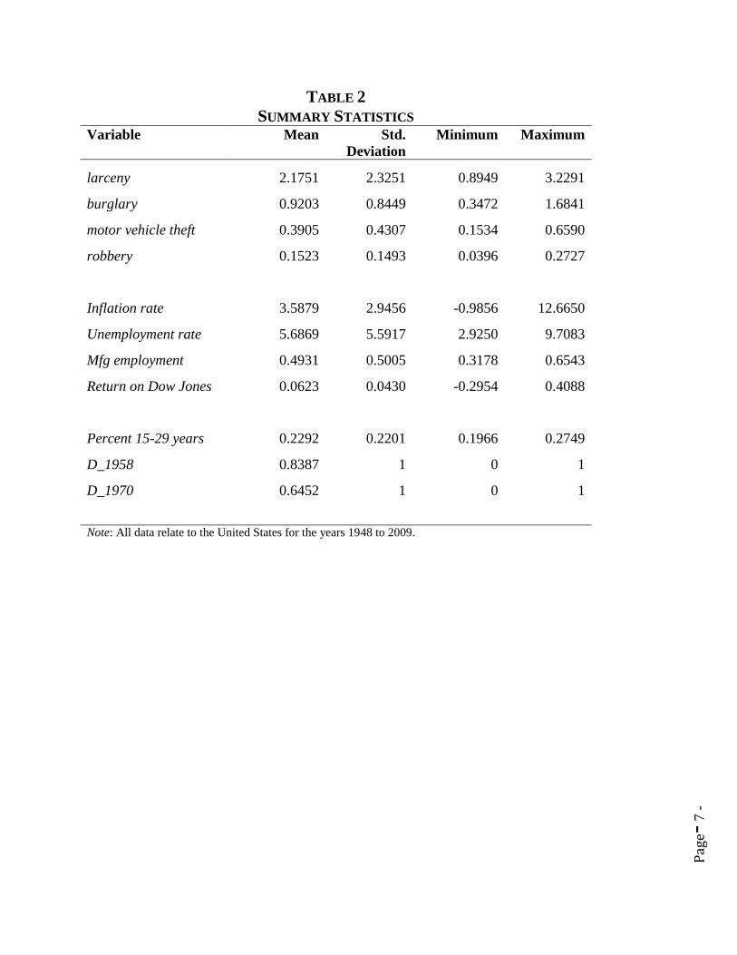
Table 1 provides variable names, definitions, and data sources. Table 2 presents summary

statistics of the variables used in the analysis. Figure 1 shows time-plots of the property crime

rates. The time-plots of the four crime rates behave similarly over time, each resembling a

bubble like series. All property crime rates rise in the 1960s, but the drop-off occurs at different

times. For example, the burglary rate drops from its peak much earlier than the other series.

Larceny is by far the largest crime category, as it is larger than the remaining three categories

combined. If all four categories were summed to an aggregate measure of property crime,

larceny would clearly dominate the results.

Because the dependent variables have some of the characteristics of a bubble series, they are

well-suited for an UCM. A bubble arises when the observable fundamental driving forces cannot

predict the magnitude of the upswing or downswing in the series. In our case, the "bubble" is the

rapid rise in the property crime rate in the 1960s and the strong decline in the 1990s. In this

study, we are interested in determining the impact on crime rates of macroeconomic influences.

These are observable fundamental drivers of property crime rates. The unobserved component

modeling allows us to decompose the crime rate into those observable factors and those

determinants, such as crime deterrence, that we know exist but are difficult to identify

theoretically or impossible to measure appropriately, especially over longer time horizons.

Time-plots for the explanatory variables are shown in Figure 2: (i) the inflation rate in the

upper-left panel, (ii) the unemployment rate in the upper-right panel, (iii) the manufacturing

employment index in the lower-left panel, and (iv) the return on the Dow Jones Industrial in the

Pag

e- 8

-

lower-right panel. A casual inspection of the trends in these variables does not reveal any

apparent relationships between them and the property crime rates. The only exception is the

inflation and unemployment rates, as these series track the changes in property crime rates

reasonably well.

As a robustness check, we include a control for the share of young people in the population

(i.e. 15-29 year-olds). The literature has stressed the importance of age composition as an

important predictor of crime (Hirschi and Gottfredson 1983; Allen 1996). However, empirical

research on the relationship between age composition and crime has produced mixed results

(Levitt 1999). Levitt (1999, 2001) argues that age composition can explain a relatively small

share of the variation in crime rates. However, a recent study using time-series data shows a

strong positive relationship between the percentage of the population aged 15-29 years and the

murder rate (Nunley et al. unpublished).

4. Econometric Methodology

The UCM decomposes each dependent variable into (a) a number of unobserved components

that are required by the particular application and (b) an observed component vector that consists

of the macroeconomic determinants of property crime and control variables identified in the last

section:8

' for 1,2,..., .t t t t ty x t T (1)

In equation (1), the parenthesis term consists of two unobserved components, a stochastic trend

(μ) and a stochastic cycle (ψ). The observed components are given by the regression vector x and

the associated coefficient vector α. The term ε is a zero mean constant variance disturbance term.

8 See Harvey (1989, 1997), Durbin and Koopman (2001) and Commandeur and Koopman (2007) for more

details on the UCM approach.

Pag

e- 9

-

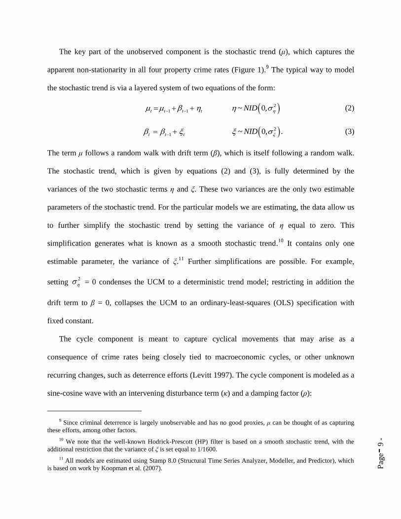
The key part of the unobserved component is the stochastic trend (μ), which captures the

apparent non-stationarity in all four property crime rates (Figure 1).9 The typical way to model

the stochastic trend is via a layered system of two equations of the form:

2

1 1 ~ 0,t t t t NID (2)

2

1 ~ 0,t t t NID . (3)

The term μ follows a random walk with drift term (β), which is itself following a random walk.

The stochastic trend, which is given by equations (2) and (3), is fully determined by the

variances of the two stochastic terms η and ξ. These two variances are the only two estimable

parameters of the stochastic trend. For the particular models we are estimating, the data allow us

to further simplify the stochastic trend by setting the variance of η equal to zero. This

simplification generates what is known as a smooth stochastic trend.10

It contains only one

estimable parameter, the variance of ξ.11

Further simplifications are possible. For example,

setting 2

= 0 condenses the UCM to a deterministic trend model; restricting in addition the

drift term to β = 0, collapses the UCM to an ordinary-least-squares (OLS) specification with

fixed constant.

The cycle component is meant to capture cyclical movements that may arise as a

consequence of crime rates being closely tied to macroeconomic cycles, or other unknown

recurring changes, such as deterrence efforts (Levitt 1997). The cycle component is modeled as a

sine-cosine wave with an intervening disturbance term (κ) and a damping factor (ρ):

9 Since criminal deterrence is largely unobservable and has no good proxies, μ can be thought of as capturing

these efforts, among other factors.

10 We note that the well-known Hodrick-Prescott (HP) filter is based on a smooth stochastic trend, with the

additional restriction that the variance of ξ is set equal to 1/1600.

11 All models are estimated using Stamp 8.0 (Structural Time Series Analyzer, Modeller, and Predictor), which

is based on work by Koopman et al. (2007).

Pag

e- 1

0 -

( ) (4)

(

) (5)

The frequency parameter ( ) determines the period in years as , and the two disturbance

terms and are uncorrelated with mean zero and common variance.

Previous studies that analyze aggregate crime rates use a variety of econometric techniques:

(i) OLS, (ii) vector autoregressions (VARs), and (iii) cointegration. In what follows, we briefly

mention some of the problems pointed out in the literature with these approaches and how the

unobserved component approach compares.

The non-stationary behavior of the crime rates over time (Figure 1) suggests that OLS can

produce spurious results, unexplainable lags on the variables, and residual series that indicate a

misspecification. Using instead first differences to eliminate the trend, as in Cantor and Land‟s

(1985) seminal paper on the effects of unemployment on aggregate crime rates, removes any

long-run relationship that may exist among the variables. It can also cause spurious relationships

among the variables to the extent they are of different order.12

In response to Cantor and Land

(1985), a number of alternative estimation techniques are used to investigate the relationship

between crime and unemployment in the short-run and long-run.

Corman et al. (1987) use a VAR approach to estimate the interrelationship between the

supply of crime in New York City and variables meant to capture changes in the business cycle,

demographic composition, and criminal deterrence. While VARs are useful for uncovering

dynamic relationships (i.e. crime and criminal deterrence) without imposing ad hoc identification

12

If the crime rate is an I(1) variable, differencing the crime rate would make it an I(0) variable. Assuming a

right-hand side variable is stationary over time, differencing this variable would result in over-differencing and

spurious estimation results.

Pag

e- 1

1 -

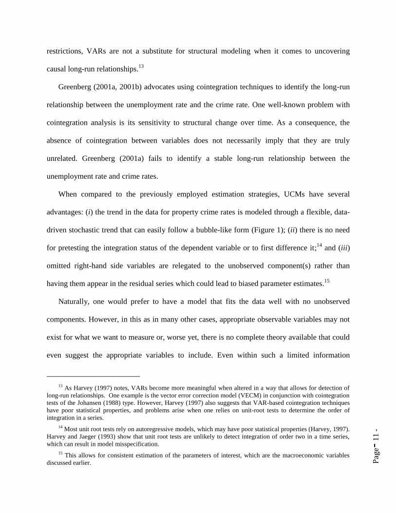
restrictions, VARs are not a substitute for structural modeling when it comes to uncovering

causal long-run relationships.13

Greenberg (2001a, 2001b) advocates using cointegration techniques to identify the long-run

relationship between the unemployment rate and the crime rate. One well-known problem with

cointegration analysis is its sensitivity to structural change over time. As a consequence, the

absence of cointegration between variables does not necessarily imply that they are truly

unrelated. Greenberg (2001a) fails to identify a stable long-run relationship between the

unemployment rate and crime rates.

When compared to the previously employed estimation strategies, UCMs have several

advantages: (i) the trend in the data for property crime rates is modeled through a flexible, data-

driven stochastic trend that can easily follow a bubble-like form (Figure 1); (ii) there is no need

for pretesting the integration status of the dependent variable or to first difference it;14

and (iii)

omitted right-hand side variables are relegated to the unobserved component(s) rather than

having them appear in the residual series which could lead to biased parameter estimates.15

Naturally, one would prefer to have a model that fits the data well with no unobserved

components. However, in this as in many other cases, appropriate observable variables may not

exist for what we want to measure or, worse yet, there is no complete theory available that could

even suggest the appropriate variables to include. Even within such a limited information

13

As Harvey (1997) notes, VARs become more meaningful when altered in a way that allows for detection of

long-run relationships. One example is the vector error correction model (VECM) in conjunction with cointegration

tests of the Johansen (1988) type. However, Harvey (1997) also suggests that VAR-based cointegration techniques

have poor statistical properties, and problems arise when one relies on unit-root tests to determine the order of

integration in a series.

14 Most unit root tests rely on autoregressive models, which may have poor statistical properties (Harvey, 1997).

Harvey and Jaeger (1993) show that unit root tests are unlikely to detect integration of order two in a time series,

which can result in model misspecification.

15 This allows for consistent estimation of the parameters of interest, which are the macroeconomic variables

discussed earlier.

Pag

e- 1

2 -

framework, however, the use of an UCM allows us, in principle, to generate believable

parameter estimates for those variables that are observable. In addition, it is sometimes possible

to derive some clues from the estimated representations of the unobserved components what

variables may likely be driving the unexplained portion of the trend in property crime rates. Such

clues may help in identifying some additional observable variables for the statistical analysis or

in making the underlying theory more precise.

5. Results

Larceny is by far the largest component of the four types of property crime we consider in

this study. Hence, movements in the larceny rate dominate the aggregate property crime rate. We

use the larceny rate to test a number of different specifications, including checking whether the

unemployment rate or manufacturing employment better captures movements in the property

crime rate.

Table 3 provides five alternative models for the larceny rate over the period 1948 to 2009.

All five models use the same unobserved component specification16

but differ in terms of the

included observable variables. Model 1 uses the standard unemployment rate as a measure of job

opportunity or the lack thereof. Model 2 is directly comparable to Model 1; it contains the well-

known SMI employment index for the manufacturing sector in lieu of the unemployment rate.

Both variables have the expected sign. However, Models 1 and 2 differ not only in their overall

goodness of fit, but also in the measured impact of several independent variables and their

statistical significance. Model 2 is the preferred model in terms of statistical fit. Both coefficients

of determination, the one around the trend (Rd2) and the overall R

2, are larger for Model 2 than

16

A smooth stochastic trend is used. It consists of a non-stochastic random walk with a drift, which follows

itself a standard random walk. This unobserved trend component is driven by only one parameter, the variance of

the random walk that is determining the drift term.

Pag

e- 1

3 -

for Model 1, and the two information criteria, Akaike (AIC) and Bayes-Schwartz (BIC), are

lower. Of the four macroeconomic variables, the return on the Dow Jones index is most affected

by switching the unemployment rate out with the manufacturing employment index. The

coefficient on the stock return rises appreciably in magnitude and becomes statistically

significant as one moves from Model 1 to Model 2. The coefficient of the inflation rate drops

somewhat and so does its statistical significance, but it remains statistically significant at the

five-percent level. Both control variables, the percentage of 15 to 29 year olds and the dummy

variable for the change in crime reporting procedures in 1958, receive lower coefficient values

and the dummy variable turns statistically insignificant.

Models 3, 4 and 5 of Table 3 provide some variation of the model specification relative to

our preferred larceny Model 2. In particular, we drop the stock market variable in Model 3,

which lowers the measured impact of both inflation and manufacturing employment on crime.

The coefficient of determination around the trend of the crime rate (Rd2) falls appreciably.

Model 4 drops instead the demographic control variable. The measured impact of all remaining

coefficients decreases and so does the explanatory power of the equation (Rd2). Model 5

removes all macroeconomic variables and leaves only the control variables in the model. The

impact of the demographic variable drops somewhat, but that of the dummy variable increases.

The equation loses a large amount of explanatory power around the trend as the Rd2 measure

falls to a fraction of its value for Model 2. Yet, we notice that the overall coefficient of

determination (R2) does not change much at all across models, which is expected for an UCM:

left-out variables are absorbed in the stochastic trend. This also explains why the coefficients of

the included variables do not change dramatically as the number of explanatory variables is

reduced. Overall, these results support the idea suggested in the methodology section: the impact

Pag

e- 1

4 -

of individual observed variables can be pinned down by UCMs even if some key variables are

missing from the equation because they are either unknown or not measurable.

Table 4 presents estimation results for burglary, motor vehicle theft, and robbery. The models

are analogous to Model 2 of Table 3. The explanatory power around the trend (Rd2) of the

included observable variables is slightly better than that for the preferred larceny model; but the

overall fit of the three models (R2) is somewhat less. The models for motor vehicle theft and

robbery use the same unobserved component model as the larceny model. The burglary model

also contains a cycle component, which is represented in Section 4 by equations (4) and (5).17

All four crime rate models (Model 2 of Table 3 and all models of Table 4) have in common

that inflation and manufacturing employment have the expected signs and are consistently

significant, although at different levels. The return on the Dow Jones price index has the positive

sign consistent with the relative deprivation or poverty theory. It is also statistically significant at

conventional levels, except for its impact on motor vehicle theft.

The impact of the two control variables on crime rates is mixed. Demographic change, as

proxied by the percentage of young adults in the population, is highly influential for larceny, but

has little perceptible influence on the rates of burglary, motor vehicle theft and robbery. A

possible explanation is that the latter three crimes require a greater investment of criminal human

capital than larceny. They may, therefore, be more likely conducted by career criminals rather

than young adults shifting into and out of property crime based on opportunistic behavior. The

1958 changes related to the collecting and processing of crime data have had a perceptible but

limited influence on the reported crime rates and their determining equations. They primarily

affect motor vehicle theft and robbery; they are not statistically significant at all for burglary,

17

We note that the cycle has a period of slightly under 6.5 years.

Pag

e- 1

5 -

which is the reason why it is left out of the final equation for this crime rate. Interestingly, the

sign of the impact is not consistent across crime rates.18

While Tables 3 and 4 focus on the statistical significance of the estimates, Table 5

emphasizes their economic significance. In particular, Table 5 converts the coefficients of Tables

3 and 4 into elasticities. For each coefficient and crime rate, four elasticities are provided, one for

the sample mean (1948-2009), and one for each of the three-year periods centered on 1960,

1980, and 2000. Table 5 reveals that the large estimated coefficients for larceny (Table 3) reflect

mostly that the larceny rate is far larger than any other crime rate, not that it reacts far more

strongly to a change in every independent variable. In fact, the elasticities of the larceny rate with

respect to the inflation rate are lower than for the other three property crime rates; the other two

elastiticies of larceny with respect to the other macroeconomic variables also tend to be on the

low side. Only the elasticity of larceny with respect to the demographic control variable is far

larger than those for the other property crime rates, which supports the earlier finding that the

percentage of young adults is only statistically significant for the larceny rate.

Table 5 also reveals a fair amount of variation in the elasticities over time. The elasticities of

the property crime rates with respect to inflation peak around the time when inflation reaches its

maximum, around 1980. At the same time, the crime rate elasticities with respect to

manufacturing employment reach a minimum. The elasticities with respect to both the return on

the Dow Jones index and the demographic control variable reach a maximum around 1960.

When the sample-average elasticities of Table 5 are combined with the percentage changes

of the average values of the dependent and independent variables (Table 6), it is possible to

18

It should be noted that the estimates for the macroeconomic variables are not materially affected by the

inclusion of the observation-specific dummy variable for 1958. The lack of sensitivity in the estimates highlights the

attractiveness of the unobserved component modeling strategy.

Pag

e- 1

6 -

gauge the relative importance of changes in the three macroeconomic variables in explaining the

observed changes in the crime rates over time. Table 7 presents such a comparison.

Table 7 presents in the first two rows the observed percentage changes in the four crime rates

based on the sample averages given in Table 6. The rise in crime rates from around 1960 to 1980

is dramatic, well over 100 percent for all four types of property crime. The predictions based on

the sample-average elasticities (Table 5) and the percentage changes of the three macroeconomic

variables as well as the demographic variable (implied by Table 6) fall significantly short of the

observed increases for three of the four crime rates. Only for the larceny rate is the predicted

increase of the correct order of magnitude. The significant underestimate of the increase in the

three other crime rates reveals that there are forces at work other than those related to

macroeconomic factors or the share of young adults in the population.19

The predictions of the

decrease in the four property crime rates from 1980 to 2000 are far better for burglary, motor

vehicle theft and robbery, but much worse for larceny.

The last seven rows of Table 7 present some numerical evidence on the extent to which the

three macroeconomic variables contribute to predicting percentage changes in the four crime

rates. The first two rows of this section of Table 7 relate the crime predictions based solely on

the macroeconomic variables to the predictions that also include the demographic variable. It is

apparent that the macroeconomic variables play only a small role in explaining the variation in

the larceny rate relative to the demographic variable. By contrast, the macroeconomic changes

between 1960 and 1980 play a sizable role in predicting the surge in burglary, motor vehicle

theft, and robbery relative to the demographic variable. But they are far less important in

explaining the downturn in the crime rates after 1980.

19

In the estimated model, these other forces are captured - although not economically explained - by the smooth

stochastic trend.

Pag

e- 1

7 -

The last five rows of Table 7 relate the predictions based on the macroeconomic variables to

the actual changes in the four crime rates. When taken together and averaged over the periods

1960 to 1980 and 1980 to 2000, the macroeconomic variables can explain about 15 percent of

the variation in the rate of motor vehicle theft. The contribution attributable to macroeconomic

variables is less for the other three property crime rates, on average about 10 percent for robbery,

9 percent for larceny, and 8 percent for burglary. The last three rows of Table 7 identify the

average contribution over the periods 1960 to 1980 and 1980 to 2000 for each of the three

macroeconomic variables. It is apparent that inflation accounts for almost all of the contribution

of the three macroeconomic variables. The contribution of manufacturing employment is hardly

noticeable and changes in the Dow Jones index appear irrelevant. These results suggest that

inflation is by far the most important macroeconomic variable that can account for variations in

property crime rates, with its impact being largest for motor vehicle theft.

6. Conclusions

This study analyzes to what extent changes in the macroeconomic environment have

contributed to changes in the rates of property crime over time. The empirical analysis is

conducted for the U.S. using annual data over the time period from 1948 to 2009. Three types of

macroeconomic variables are considered: the rate of inflation, employment in manufacturing,

and the rate of return on the Dow Jones stock price index. Four property crime rates are

investigated: larceny, burglary, motor vehicle theft, and robbery. The empirical analysis relies on

unobserved component models, also known as structural time series models. These models are

particularly useful for the analysis of crime rates over time because they generate meaningful

estimates of the role played by macroeconomic variables in determining property crime rates

even though our empirical models do not explicitly include measures of crime deterrence. By

Pag

e- 1

8 -

excluding variables for crime deterrence, we avoid the well-known issues associated with

endogeneity and lack of consistent data. In addition, we avoid the problems normally associated

with omitted variables in the context of standard estimation techniques, such as ordinary least

squares, by implicitly accounting for their influence through the specification of unobserved

components.

We find that our three macroeconomic variables have, on average, a statistically significant

impact on the four rates of property crime and in the expected direction. In particular, a rise in

inflation increases property crime rates, so does a decrease in manufacturing employment and an

increase in the annual return on the Dow Jones stock price index. We determine that our

manufacturing employment index fits the data better than the commonly used unemployment

rate. We also show that the percentage of young adults in the population significantly affects the

larceny rate, but that it has no statistical significance for the burglary, motor vehicle theft and

robbery rates. All property crime rates except the burglary rate are also significantly affected by

the change in crime reporting standards in 1958, although not all in the same direction.

In determining the economic significance of our findings, we examine to what extent the

surge in property crime rates from 1960 to the 1980s or their subsequent decline can be predicted

by the observed changes in our macroeconomic variables given our estimated crime rate

elasticities. We find that all three macroeconomic variables combined can, on average, explain

about 15 percent of the observed change in motor vehicle theft, and less of the change in other

property crime rates (10 percent for robbery, 9 percent for larceny and 8 percent for burglary). If

one asks which of our three macroeconomic variables has the most impact, the answer leaves no

room for interpretation. Almost all of the impact of the three macroeconomic variables falls on

the inflation rate. The predictive content of manufacturing employment is negligible and the

Pag

e- 1

9 -

impact of the return on the Dow Jones index is hardly noticeable. We conclude that containing

inflation is the key contribution of macroeconomics for the stabilization of property crime.

REFERENCES

Allen, Ralph C., (1996). 'Socioeconomic Conditions and Property Crime: A Comprehensive

Review and Test of the Professional Literature', American Journal of Economics and

Sociology, Vol. 55, pp. 293-308.

Becker, G. (1968). „Crime and Punishment: An Economic Approach‟, Journal of Political

Economy, Vol. 76, pp. 169-217.

Burtless, G. (1990a). „Introduction and Summary‟, in Burtless G. (ed.), A Future of Lousy Jobs:

The Changing Structure of U.S. Wages, The Brookings Institution, Washington, pp. 1-30.

Burtless, G. (1990b). „Earnings Inequality over the Business and Demographic Cylces‟, in

Burtless G. (ed.), A Future of Lousy Jobs: The Changing Structure of U.S. Wages, The

Brookings Institution, Washington, D.C., pp. 77-122.

Cantor, D. and Land, K. (1985). „Unemployment and Crime Rates in the Post-World War II

United States: A Theoretical and Empirical Analysis‟. American Sociological Review, Vol.

50, pp. 317-332.

Christiano, L. J., Eichenbaum, M., and Evans, C. L. (2005). „Nominal Rigidities and the

Dynamic Effects of a Shock to Monetary Policy‟, Journal of Political Economy, Vol. 113,

pp. 1-45.

Commandeur, J.J.F and Koopman, S.J. (2007). An Introduction to State Space Time Series

Analysis. Oxford and New York, Oxford University Press.

Corman, H., Joyce, T., and Lovitch, N. (1987). „Crime, Deterrence, and the Business Cycle in

New York City: A VAR Approach‟, Review of Economics and Statistics, Vol. 69, pp. 695-

700.

Pag

e- 2

-

Corman, H. and Mocan, N. (2000). „A Time-Series Analysis of Crime, Deterrence, and Drug

Abuse in New York City‟, American Economic Review, Vol. 90, pp. 584-604.

Chester, R.C., (1976). 'Perceived Relative Deprivation as a Cause of Property Crime.' Crime and

Delinquency, Vol. 22, pp. 17-30.

Deutsch, J., Spiegel, U., and Templeman, J. (1992). 'Crime and Economic Inequality: An

Economic Approach.' Atlantic Economic Journal, Vol. 20, pp. 46-54.

Devine, J., Sheley, J., and Smith, M. (1988). „Macroeconomic and Social-Control Policy

Influences on Crime Rate Changes, 1948-1985‟, American Sociological Review, Vol. 53, pp.

407-420.

DiIulio, J.J. (1996). „Help Wanted: Economists, Crime and Public Policy‟, Journal of Economic

Perspectives, Vol. 10, pp. 3-24.

Durbin, J. and Koopman, S.J. (2001). Time Series Analysis by State Space Methods. Oxford and

New York, Oxford University Press.

Ehrlich, I., (1973). 'Participation in Illegitimate Activities: A Theoretical and Empirical

Investigation.' Journal of Political Economy, Vol. 81, pp. 521-64.

Gould, E., Weinberg, B., and Mustard, D. (2002). „Crime Rates and Local Labor Market

Opportunities in the United States: 1979-1997‟, Review of Economics and Statistics, Vol. 84,

pp. 45-61.

Greenberg, D. (2001a). „Time Series Analysis of Crime Rates‟, Journal of Quantitative

Criminology, Vol. 17, pp. 291-327.

Greenberg, D. (2001b). „On Theory, Models, Model-Testing, and Estimation‟ Journal of

Quantitative Criminology, 17(4): 409-422.

Pag

e- 3

-

Grogger, J. (1992). „Arrests, Persistent Youth Joblessness, and Black/White Employment

Differentials‟, Review of Economics and Statistics, Vol. 71, pp. 100-106

Grogger, J. (1998). „Market Wages and Youth Crime‟, Journal of Human Resources, Vol. 16,

pp. 756-791.

Harvey, A. (1989). Forecasting Structural Time Series Models and the Kalman Filter,

Cambridge University Press, Cambridge.

Harvey, A. (1997). „Trends, Cycles, and Autoregressions‟, Economic Journal, Vol. 107, pp. 192-

201.

Harvey, A. and Jaeger, A. (1993). „Detrending, Stylized Facts and the Business Cycle‟, Journal

of Applied Econometrics, Vol. 8, pp. 31-47.

Hirschi, T. and Gottfredson, M. (1983). 'Age and the Explanation of Crime.' American Journal of

Sociology, Vo.l. 89, pp. 552-584.

Johansen, S. (1988). „Statistical Analysis of Cointegration Vectors‟ Journal of Economic

Dynamics and Control, Vol. 12, pp. 131-154.

Kelly, M. (2000). „Inequality and Crime‟, Review of Economics and Statistics, Vol. 82, pp. 530-

539.

Koopman S., Harvey, A., Doornik, J. and Shephard, N. (2000). Stamp: Structural Time Series

Analyzer, Modeller, and Predictor, Timberlake Consultants Press, London.

Land, K.C., and Felson, M. (1976). 'A General Framework for Building Macro Social Indicator

Models: Including an Analysis of Changes in Crime Rates and Police Expenditures',

American Journal of Sociology, Vol. 82, pp. 564-604.

Levitt, S. (1996). „The Effect of Prison Population Size on Crime Rates: Evidence from Prison

Overcrowding Litigation‟, Quarterly Journal of Economics, Vol. 111, pp. 319-351.

Pag

e- 4

-

Levitt, S. (1997). „Using Electoral Cycles in Police Hiring to Estimate the Effect of Police on

Crime‟, American Economic Review, Vol. 87, pp. 270-290.

Levitt, S. (1998a). „Why Do Increased Arrest Rates Appear to Reduce Crime: Deterrence,

Incapacitation, or Measurement Error?‟, Economic Inquiry, Vol. 36, pp. 353-372.

Levitt, S. (1998b). „The relationship between crime reporting and police: Implications for the use

of uniform crime reports‟, Journal of Quantitative Criminology, Vol. 14, pp. 61-81.

Levitt, S. (1999). "The Limited Role of Changing Age Structure in Explaining Aggregate Crime

Rates." Criminology 37, no. 3: 581-597.

Levitt, S. (2001). „Alternative Strategies for Identifying the Link Between Unemployment and

Crime‟, Journal of Quantitative Criminology, Vol. 17, pp. 377-390.

Myers, S. (1983). „Estimating the Economic Model of Crime: Employment Versus Punishment

Effects‟, The Quarterly Journal of Economics, Vol. 98, pp. 157-166.

Nunley, J.M., Seals Jr., R.A., and Zietz, J. (2011). „Demographic Change, Macroeconomic

Conditions, and the Murder Rate: The Case of the United States, 1934 to 2006‟, unpublished.

Stiles, B.L., Liu, X., and Kaplan, H. (2000). 'Relative Deprivation and Deviant Adaptations: The

Mediating Effects of Negative Self-Feelings', Journal of Research in Crime and

Delinquency, Vol. 37, pp. 64-90.

Tang, C.F., and Lean, H.H. (2009). „New Evidence from the Misery Index in the Crime

Funcion.‟ Economics Letters Vol. 102, pp. 112-115.

Walker, Iain and Smith, Heather J., (2001). Relative Deprivation: Specification, Development,

and Integration, Cambridge University Press.

Pag

e- 5

-

Williams, J. and Sickles, R. (2002). „An Analysis of the Crime as Work Model: Evidence from

the 1958 Philadelphia Birth Cohort Study‟. Journal of Human Resources, Vol. 37, pp. 479-

509.

Wilson, J. and Herrnstein, R. (1985). Crime and Human Nature. Simon and Schuster, New York,

NY.

Wilson, W. (1987). The Truly Disadvantaged: The Inner City, the Underclass, and Public

Policy, University of Chicago Press, Chicago, IL.

Wilson, W. (1996). When Work Disappears: The World of the New Urban Poor, Alfred A.

Knopf, Inc., New York, NY.

Pag

e- 6

-

TABLE 1

VARIABLE NAMES AND VARIABLE DEFINITIONS

Variable Variable Definition

larceny Larceny rate of the population per 100,000

burglary Burglary rate of the population per 100,000

motor vehicle theft

robbery Robbery rate of the population per 100,000

Inflation rate Log difference of the Consumer Price Index

Unemployment rate Percentage of workforce that is unemployed

Mfg employment Supply Management Institute (SMI) manufacturing employment

index (napmei)

Return on Dow Jones Log difference of Dow Jones stock price index

Percent 15-29 years percent of the population in the age bracket 15 to 29

D_1958 0/1 variable, 1 from 1958 onward

D_1970 0/1 variable, 1 from 1970 onward

Notes: All property crime rates come from the FBI‟s Uniformed Crime Report. The other variables all come

from the Bureau of Labor Statistics (BLS).

Pag

e- 7

-

TABLE 2

SUMMARY STATISTICS

Variable Mean Std.

Deviation

Minimum Maximum

larceny 2.1751 2.3251 0.8949 3.2291

burglary 0.9203 0.8449 0.3472 1.6841

motor vehicle theft 0.3905 0.4307 0.1534 0.6590

robbery 0.1523 0.1493 0.0396 0.2727

Inflation rate 3.5879 2.9456 -0.9856 12.6650

Unemployment rate 5.6869 5.5917 2.9250 9.7083

Mfg employment 0.4931 0.5005 0.3178 0.6543

Return on Dow Jones 0.0623 0.0430 -0.2954 0.4088

Percent 15-29 years 0.2292 0.2201 0.1966 0.2749

D_1958 0.8387 1 0 1

D_1970 0.6452 1 0 1

Note: All data relate to the United States for the years 1948 to 2009.

Pag

e- 8

-

TABLE 3

MODEL RESULTS FOR THE LARCENY RATE

Variables Model 1 Model 2 Model 3 Model 4 Model 5

Inflation rate 0.0188 0.0123 0.0093 0.0108

[0.002] [0.037] [0.125] [0.085]

Unemployment rate 0.0323

[0.008]

Mfg employment

-0.5000 -0.3570 -0.4682

[0.000] [0.008] [0.002]

Return on Dow Jones 0.0486 0.1237

0.1190

[0.236] [0.010]

[0.018]

Percent 15-29 years 37.1471 32.6926 32.4086

27.3278

[0.002] [0.003] [0.005]

[0.027]

D_1958 -0.2665 -0.1332 -0.1578 -0.0911 -0.1753

[0.003] [0.108] [0.066] [0.287] [0.044]

Rd2 0.3933 0.4238 0.3373 0.3107 0.1527

R2 0.9855 0.9863 0.9842 0.9836 0.9806

AIC -4.3380 -4.3895 -4.3003 -4.2610 -4.1711

BIC -4.0635 -4.1150 -4.0602 -4.0208 -3.9995

DW 2.154 2.050 2.081 2.060 1.970

p-values:

Normality 0.773 0.932 0.293 0.010 0.154

Heteroskedasticity 0.960 0.948 0.983 0.982 0.908

Notes: all models contain a smooth stochastic trend, i.e. a combination of fixed level and stochastic

slope. See the discussion in the text on the details. P-values are provided in brackets below the

coefficient estimates. The estimates relate to the United States for the years 1948 to 2009.

Variables are defined in Table 1.

Pag

e- 9

-

TABLE 4

MODEL RESULTS FOR BURGLARY, MOTOR VEHICLE THEFT,

AND ROBBERY

Variables Burglary Motor

Vehicle Theft Robbery

Inflation rate 0.0069 0.0029 0.0018

[0.054] [0.028] [0.012]

Mfg employment -0.3439 -0.0619 -0.0719

[0.000] [0.049] [0.000]

Return on Dow Jones 0.0648 0.0171 0.0122

[0.042] [0.135] [0.038]

Percent 15-29 years 4.6032 1.2965 0.9840

[0.129] [0.568] [0.411]

D_1958

-0.0395 0.0267

[0.044] [0.009]

Rd2 0.5280 0.4749 0.4407

R2 0.9843 0.9790 0.9766

DW 1.563 1.960 1.879

p-values:

Normality 0.091 0.184 0.289

Heteroskedasticity 0.089 0.938 0.315

Notes: all models contain a smooth stochastic trend, i.e. a combination of fixed level and

stochastic slope. The burglary model contains in addition a stochastic cycle component. See the

discussion in the text on the details. P-values are provided in brackets below the coefficient

estimates. The estimates relate to the United States for the years 1948 to 2009.

Pag

e- 1

0 -

Table 5

Economic Interpretation of Preferred Crime Rate Models

Crime Rate Elasticities

Driving variable Larceny Burglary Motor Robbery

vehicle theft

Inflation rate

evaluated at:

sample mean 0.020 0.027 0.027 0.042

average of 1959-61 0.013 0.016 0.017 0.035

average of 1979-81 0.044 0.047 0.065 0.082

average of 1999-01 0.014 0.025 0.019 0.034

Mfg employment

evaluated at:

sample mean -0.113 -0.184 -0.078 -0.233

average of 1959-61 -0.234 -0.352 -0.159 -0.628

average of 1979-81 -0.075 -0.099 -0.058 -0.138

average of 1999-01 -0.093 -0.214 -0.068 -0.226

Return on Dow Jones

evaluated at:

sample mean 0.004 0.004 0.003 0.005

average of 1959-61 0.013 0.015 0.010 0.025

average of 1979-81 0.002 0.002 0.002 0.003

average of 1999-01 0.003 0.005 0.002 0.004

Percent 15-29 years

evaluated at:

sample mean 3.445 1.146 0.761 1.481

average of 1959-61 5.827 1.792 1.268 3.272

average of 1979-81 2.889 0.781 0.719 1.111

average of 1999-01 2.716 1.282 0.640 1.385

Notes: The elasticities use the estimated coefficients of Model 2 (Table 3) and of the

models of Table 4. These coefficients are multiplied by the sample values of the driving

variables (left column) and divided by the corresponding values of the dependent variable.

Pag

e- 1

1 -

Table 6

Average Values of Dependent and Independent Variables over Time

Variables

Sample

Mean

Average

1959-61

Average

1979-81

Average

1999-01

Dependent Variables

Larceny 2.175 1.104 3.102 2.505

Burglary 0.920 0.505 1.615 0.747

Motor vehicle theft 0.391 0.201 0.494 0.422

Robbery 0.152 0.059 0.243 0.148

Independent Variables

Inflation rate 3.588 1.158 11.068 2.753

Mfg employment 0.493 0.517 0.465 0.464

Return on Dow Jones 0.062 0.119 0.059 0.053

Percent 15-29 years 0.229 0.197 0.274 0.208

Notes: See Table 1 for variable definitions and Table 2 for basic statistics over the complete sample.

Pag

e- 1

2 -

Table 7

Actual and Predicted Percentage Changes of Crime Rates

And Percentage Contribution of Macroeconomic Variables

Time

Horizon Larceny Burglary

Motor

vehicle theft Robbery

% change

Actual crime rates 1960-80 1.81 2.20 1.46 3.10

1980-00 -0.19 -0.54 -0.15 -0.39

Predicted rates based

on all variables

1960-80 1.54 0.70 0.53 0.97

1980-00 -0.85 -0.30 -0.20 -0.39

Predicted rates based

on macro variables only

1960-80 0.18 0.25 0.24 0.38

1980-00 -0.02 -0.02 -0.02 -0.03

% contribution of

macro variables

in generating predicted

crime rate changes 1960-80 0.12 0.35 0.44 0.40

1980-00 0.02 0.07 0.10 0.08

in predicting actual 1960-80 0.10 0.11 0.16 0.12

crime rate changes 1980-00 0.08 0.04 0.14 0.08

% contribution of

individual variables

Inflation rate average of 0.088 0.071 0.147 0.099

Mfg employment 1960-80 & 0.003 0.004 0.002 0.003

Return on Dow Jones 1980-00 0.000 0.000 0.000 0.000

Notes: predictions use mean elasticities, as given in Table 5, and percentage changes as given in Table 6.

Unobserved components are not used for any of the predictions. Therefore, differences between actual and predicted

values reflect the impact of estimated unobserved components and random noise.

Pag

e- 1

3 -

FIGURE 1: PROPERTY CRIME RATES OVER TIME

Note: The y-axis measures the various property crime rates per 100,000 persons.

0.5

1

1.5

2

2.5

3

3.5

1948 1958 1968 1978 1988 1998 2008

larceny

0.2

0.4

0.6

0.8

1

1.2

1.4

1.6

1.8

1948 1958 1968 1978 1988 1998 2008

burglary

0.1

0.2

0.3

0.4

0.5

0.6

0.7

1948 1958 1968 1978 1988 1998 2008

motor vehicle theft

0

0.05

0.1

0.15

0.2

0.25

0.3

1948 1958 1968 1978 1988 1998 2008

robbery

Pag

e- 1

4 -

FIGURE 2: EXPLANATORY MACROECONOMIC VARIABLES OVER TIME

Note: variable definitions are provided in Table 1.

-2

0

2

4

6

8

10

12

14

1948 1958 1968 1978 1988 1998 2008

inflation rate

2

3

4

5

6

7

8

9

10

1948 1958 1968 1978 1988 1998 2008

unemployment rate

0.3

0.35

0.4

0.45

0.5

0.55

0.6

0.65

0.7

1948 1958 1968 1978 1988 1998 2008

mfg employment

-0.3

-0.2

-0.1

0

0.1

0.2

0.3

0.4

0.5

1948 1958 1968 1978 1988 1998 2008

return on Dow Jones

Pag

e- 1

5 -

For Review Purposes Only

For those unfamiliar with the econometric methodology employed in this study, we also offer

some alternative estimates via ARMAX modeling. We consider these models to be inferior in

quality relative to the unobserved component models in the paper. But the parameter estimates

show a significant degree of similarity, at least in terms of order of magnitudes, to those of the

unobserved component models.

Appendix Table 1

Model Estimates by ARMAX Method

Variables Larceny Burglary Motor Robbery

vehicle theft

Inflation rate 0.0110 0.0093 0.0034 0.0022

[0.067] [0.009] [0.030] [0.002]

Mfg employment -0.3025 -0.3847 -0.0320 -0.0393

[0.019] [0.000] [0.359] [0.030]

Return on Dow Jones 0.0761 0.0834 0.0160 0.0037

[0.068] [0.017] [0.149] [0.496]

Percent 15-29 years 12.0336 7.4955 0.2742 0.9212

[0.009] [0.000] [0.803] [0.061]

D_1958 -0.1779

-0.0571 0.0257

[0.019]

[0.006] [0.002]

AR(1) 0.9833 0.9822 0.9769 0.9456

[0.000] [0.000] [0.000] [0.000]

MA(1) 0.6745

0.5238 0.6075

[0.000]

[0.000] [0.000]

constant -0.7063 -0.8242 0.2726 -0.0801

[0.564] [0.070] [0.325] [0.486]

Notes: all estimates are based on ARMAX models; the error terms are

specified as ARMA(1,1) models, except for the burglary equation, for

which an AR(1) suffices. P-values are provided below the coefficient

estimates.