School of Economics and Political Science, Department of Economics

University of St. Gallen

Shirk or Work? On How Legislators

React to Monitoring

Katharina E. Hofer

August 2016 Discussion Paper no. 2016-16

Editor: Martina Flockerzi University of St.Gallen School of Economics and Political Science Department of Economics Bodanstrasse 8 CH-9000 St. Gallen Phone +41 71 224 23 25 Fax +41 71 224 31 35 Email seps@unisg.ch

Publisher: Electronic Publication:

School of Economics and Political Science Department of Economics University of St.Gallen Bodanstrasse 8 CH-9000 St. Gallen Phone +41 71 224 23 25 Fax +41 71 224 31 35 http://www.seps.unisg.ch

Shirk or Work? On How Legislators React to Monitoring 1

Author’s address: Katharina E. Hofer Swiss Institute for Empirical Economic Research (SEW-HSG) Varnbüelstrasse 14 CH-9000 St.Gallen Phone +41 71 224 2320 Fax +41 71 224 2302 Email katharina.hofer@unisg.ch Website www.sew.unisg.ch

1 I thank the Swiss Parliamentary Services and in particular Martin Städeli for their support during the data

collection. I am grateful for comments received from Monika Bütler, Winfried Königer and Lukas Schmid, as

well as participants at the Annual Congress of the Swiss Society of Economics and Statistics.

Abstract

Does transparency affect the decision to shirk or work? The question is analyzed using the

example of parliamentary voting. Without transparency, politicians have little incentive to

attend all votes in parliament. But if voters have means to monitor their representatives'

effort, incumbents face the trade-off between shirking and deteriorating reelection prospects

the more votes they miss.

A 2014 institutional change in the Swiss Upper House allows testing the theoretical

prediction. The introduction of an electronic voting system involved individual decisions on

several types of votes to be automatically published whereas all other votes remained secret

to the public. Pre- and post-reform attendance during secret votes comes from video

recordings of all sessions. This variation in monitoring depending exogenously on vote types

allows identifying a causal effect of monitoring on shirking measured by attendance.

Legislators shirk less once attendance is monitored. The effect is particularly strong among

politicians for whom reelection is most valuable: incumbents aspiring for another term, full-

time politicians who devoted themselves to a career in parliament, and legislators with few

interest groups.

Keywords

Shirking; Absence; Monitoring; Transparency; Parliament; Legislators; Accountability

JEL Classification

D72, P16

1 Introduction

Voting and absenteeism during parliamentary sessions are the legislative analogues to working andshirking. Voting in parliament belongs to the legislators’ duties and requires their presence inthe chamber.1 However, when the media display pictures of half-empty assemblies this violatesthe “ideal” picture of the dutiful member of parliament. Attempts to count presence during leg-islative sessions document politicians missing considerable shares of votes: a third of all votes inItaly (Gagliarducci, Nannicini & Naticchioni 2010), 31% in the UK House of Commons (Besley &Larcinese 2011), and 8% in the German Bundestag (Arnold, Kauder & Potrafke 2014).

By democratic design, the electoral connection between voters and representatives is character-ized as a principal-agent relationship (Besley 2006). Legislators are thought of as accountable totheir electorate (Persson & Tabellini 2000). The form of accountability considered in this paper ispresence in parliament and participatory shirking defines departures from it (Rothenberg & Sanders2000).2

Attendance rates are calculated from official voting records. Whether participatory shirkingcan be detected thus hinges upon absences being recorded and readily accessible. If voting recordsare publicly unavailable and parliamentary minutes undisclosed, there is no way of controlling thelegislators’ behavior. Regulation regarding transparency of legislators’ behavior varies stronglyby assembly (Hug 2010; Hug, Wegmann & Wüest 2015): 25% of 92 parliaments are completelynontransparent, while all voting records are public in 22% of the assemblies and the remainderpublishes votes with some restrictions.

I address the question whether the possibility to track legislators’ presence during voting sessionsimpacts their dutifulness or effort measured by attendance rates. Absenteeism can be either excusedfor an entire day or selective: though legislators appear at the beginning of a meeting, they leavetheir seats during debates and speeches only to return for some of the votes. In the meantime, theyuse their time for communication with interest groups, work unrelated to politics or leisure.

Intuitively, if legislators cannot be detected while shirking, they have little incentive to attendall voting sessions. They will resort to participating in the most important votes but leave outless crucial ones. But if voters have the means to find out about politicians not fulfilling theirrepresentative duties, it is possible to punish shirking legislators. E.g., low attendance rates canbe negatively publicized by the press and ultimately, voters might choose not to reelect politicianswho put little effort into their representative function. This rationale is particularly appealingin settings allowing for earning non-political rents. Examples are the pursuit of a non-politicaloccupation, or fostering relationships with interest groups. Both might offer more attractive rentsthan participating in votes either in the short run or with the view to a post-political career.

In my model, I capture this intuition. Politicians allocate their time between doing political

1 Though political work also happens in committees outside the chamber, a member of parliament absent during avote cannot fulfill his representative duty.

2 Accountability or shirking can take many forms. Legislators are thought of as representing electoral preferences.Violating the electoral connection by voting against constituency interest is known as ideological shirking.

work in the chamber or shirking to earn non-political rents. Voters decide whether to reelectincumbents for a second term or replace them with a new politician. Legislators face the trade-offbetween shirking during the first term and getting reelected for a second one. The model showsthat while legislators with low non-political rents never shirk, attendance of legislators with highopportunity costs of doing politics depends on monitoring. In theory better monitoring leads tomore attendance on average. Part of the high-ability politicians optimally devote their time towork during their first term to secure reelection. Top-ability types, in contrast, have such highopportunity costs that they prefer shirking in the first term even though they are not gettingreelected for this. On average, the model predicts lower absence rates as a consequence of votetransparency. The effect should be small when legislators face their last term.

My model combines elements of the moonlighting model by Gagliarducci, Nannicini and Nat-icchioni (2010) and Besley’s (2004) optimal political wage model. Gagliarducci, Nannicini andNaticchioni (2010) extend the candidate selection literature (Caselli & Morelli 2004) by explicitlyallowing for earning ability-dependent wages in the private sector while holding a seat in parlia-ment. The main difference to their model lies in the modeling of attendance monitoring and howthat affects the electoral connection via reelection probabilities. In that my model spans overtwo political terms and thus one reelection decision, it shares similarities with Besley (2004) whowas mainly concerned with the effect of political salaries on implementing policies desirable to theelectorate.

I test the model predictions suggesting that legislators adjust their vote attendance dependingon the monitoring technology at the hands of their constituencies. I exploit an institutional changein the voting procedure of the Swiss Upper House, the Ständerat, which enhanced monitoring oflegislators for several legally defined types of votes but kept transparency constant for the remainingones. Before 2014 members of the Swiss Upper House voted exclusively by show of hands. Thepossibility of recorded votes on request was virtually never made use of. Though all sessions werevideo recorded, neither the media nor researchers have undertaken the effort of finding out aboutattendance rates in this chamber.3

Beginning in 2014, all votes in the Upper House are taken electronically. Individual decisions onseveral types of votes - emergency votes, debt brakes, ensemble votes, and final passage votes - areautomatically published online in pdf format. Monitoring legislators’ attendance has consequentlybeen facilitated for these vote types. Indeed, the independent policy platform Politnetz startedpublishing attendance rates of the Upper House on their webpage. In contrast and importantly forthis paper, the remaining vote types stay undisclosed to the public and are concealed from the eyesof the voters. Comparing the two types of votes before and after the change in voting rules allowsestimating a causal effect of monitoring on attendance rates during parliamentary voting sessionsusing a difference-in-difference estimator.

Since the change occurred in the middle of the 2011-2015 legislative period, the parliament’s

3 In contrast, the Swiss media report on attendance rates in the Lower House which takes all votes electronically andis consequently easily traceable.

4

composition remained largely unchanged. It is therefore possible to compare the same politiciansvoting under exogenously varying monitoring technologies while shutting down candidate-selectionmotifs. Moreover, the Swiss setting is ideal to test the model because Swiss Members of Parliamentare allowed to hold an occupation next to their position in parliament, and are affiliated with manyinterest groups.

The results confirm the theoretical expectations: the probability of being absent decreases frominitial levels of 19% by 3 percentage points if attendance is monitored. Legislators are more likelyto vote if shirking can be detected. The effects are particularly strong for subgroups of politicianstheoretically expected to be more accountable to their electorate. Legislators standing for reelectionshirk less but retiring politicians are not affected by the change in monitoring. Full-time politiciansreduce their absences considerably, whereas no effect can be found for legislators with outsideoccupations. Career politicians are dependent on reelection due to lack of alternative careers andmay thus react more responsive to monitoring. Legislators simultaneously employed in the privatesector, in contrast, have better outside options if their political mandate is terminated. Moreover,I find that legislators with only few interest groups reduce their absences significantly more thanlegislators with many interest groups. A potential interpretation is that interest groups as insidersto the political process have been more able to monitor “their” legislators even without recordedvoting. In contrast, legislators with few interest groups feel a stronger effect of monitoring.

This paper extends the literature dealing with effects of transparency on legislative behavior.It contributes to a better understanding of whether and how monitoring and observability affectthe way individuals behave (e.g., Benesch, Bütler and Hofer 2015; Fox 2007; Grossman and Hanlon2014; Prat 2005). Its main contribution is to exploit exogenous variation in the regulation regardingrecorded voting according to vote types and over time which allows estimating a causal effect.

The relevance of the results extends beyond the field of political economy towards areas in whichtransparency plays a role. Examples are among others labor economics and the setting of optimalwages (e.g., Barmby, Sessions & Treble 1994; Shapiro & Stiglitz 1984), or the communication ofmonetary policy decision-making processes (Gersbach & Hahn 2004, 2008).

The literature is reviewed and related to this paper in Section 2. Section 3 presents the theoret-ical model. The institutional setup and description of the data are in Section 4. The identificationstrategy is explained in Section 5. Results are reported in Section 6. Section 7 concludes.

2 Related Literature

Politicians are elected representatives of their constituencies. Empowered by their voters, they arethought of as accountable to their electorate in the spirit of a principal-agent relationship (Besley2004). This paper relates to literature on legislative accountability in general, and the role oftransparency.4

4 Bender and Lott (1996) provide literature review concerning the early foundations of this literature.

5

The principal-agent (or voter-legislator) relationship can be viewed from the angle of moralhazard or adverse selection. The role of transparency on moral hazard has been studied in anumber of contributions. In Holmström’s (1979) seminal contribution principals benefit from moreinformation on their agents’ actions. A more recent strand of the literature emphasizes potentiallyadverse effects of transparency (e.g., Gersbach & Hahn 2004; Prat 2005). Most research focuses onthe quality of outcomes resulting from public and secret voting (Mattozzi & Nakaguma 2016).

Closely to this paper, Benesch, Bütler and Hofer (2015) focus on a different aspect of the sameintroduction of electronic voting in the Swiss Upper House as in this paper. Concentrating on finalpassage votes, they investigate how transparency impacts party loyalty. They find more voting inaccordance with party lines once individual voting decisions become observable.

Other research is concerned with the effort invested in decision-making. Gersbach and Hahn(2012) show that transparency benefits the principal through better outcomes induced by theagent’s higher effort levels.

Adverse selection in agency models is at the heart of some candidate selection model. Rentsfrom being a politician determine whether a citizen becomes a candidate or not. Caselli andMorellis’ (2004) model predicts low-quality politicians because only those with low potential wageson the private market find it lucrative to earn political wages (. Gagliarducci, Nannicini andNaticchioni (2010) model legislators who additionally earn wages outside their political occupation,i.e., they moonlight. The authors provide evidence for their model mechanisms predicting high-ability candidates (as they can continue working on the private market), who, however, put lesseffort (in thems of floor voting) into their political mandate as a consequence of other activities.Fedele and Naticchioni (2015) distinguish between ability and motivation such that citizens fittingwell into public occupation receive higher intrinsic rewards from following such a profession. Datafrom Italy support their model showing that politicians who held some prior political appointmentare less likely to be absent than politicians with initial employment on the private market.

Grossman and Hanlon (2014) combine elements of moral hazard with adverse selection. Theymodel the effect of monitoring on leader effort in small communities, which is required to producea public good in combination with ability. While more monitoring positively impacts effort, itreduces average ability through adverse candidate selection, resulting in a u-shape relation betweenmonitoring intensity and the amount of the public good. They conclude that monitoring is notstrictly beneficial to the public.

My model is directly linked to the moral hazard literature as it models agents’ actions dependingon information available to the principal. If observability improves for a given set of incumbents,it is predicted to increase effort. Importantly, I also show that the setting is compatible withcandidate selection if elections take place under no transparency.

The model shares similarities with Gersbach and Hahn (2012), monitoring is beneficial to theprincipal but detrimental to agents who have to exert more effort.5 I discuss efficiency of trans-

5 In Gersbach and Hahn (2012) legislators choose higher effort so that they are perceived as competent by the voters.In my model voters have preferences over effort itself.

6

parency from an empirical view more closely in the results section.Most of the above-mentioned literature on transparency and monitoring is theoretical. Empir-

ical investigations in the above-mentioned literature rely mostly on panel or cross-sectional dataanalysis. The quasi-experimental setting in this paper constitutes a major advantage over pre-vious examinations. It exploits exogenous variation in monitoring and allows capturing a causalrelationship between transparency and effort.

This paper complements the literature exploring the determinants of effort and presence inparliament. Research has most prominently focused on the impact of salaries (Fisman et al. 2015;Mocan & Altindag 2013), outside earnings6 (Arnold, Kauder & Potrafke 2014; Gagliarducci, Nan-nicini & Naticchioni 2010), electoral competition (Bernecker 2014; Galasso & Nannicini 2011), andinstitutions (Gagliarducci et al. 2011) on participation in floor voting.

3 Theory

I draw from the theoretical framework of Gagliarducci, Nannicini and Naticchioni (2010) in whichpoliticians optimally choose how to allocate their time between work in the chamber and outsideactivities earning non-political rents. Their focus is on candidate selection. I extend their modelby introducing voter preferences over the legislators’ choice to shirk or work. My model is differentin that legislators have to consider whether voters are aware of their effort and how that impactsreelection prospects. My model spans over two legislative periods and models the threat of (no)reelection. It derives different predictions from the previous literature.

I begin with a baseline model temporarily disregarding candidate selection for the moment,and assuming that all potential candidates are willing to run for office. It allows me to isolateequilibrium behavior of elected legislators who unexpectedly get exposed to more monitoring bytheir constituencies. In a model extension, I deal with the issue of candidate selection and showunder which conditions model predictions remain unchanged.

3.1 Model Setup

Voters elect their representatives by a random draw from the pool of candidates. Legislators canstand for at most one reelection. Consequently, they are either in their first or second electoralterm, which is denoted by e ∈ [1, 2]. Future payoffs are discounted with factor β.

The only decision legislators make is what share of their time te ∈ [0, 1] in term e to allocateto work in parliament. The remainder is used for non-political work. Politicians thus face a timeconstraint which restricts their choice between political and outside work.

Legislator types α are uniformly distributed on [0, α]. The notion of type used in this modelrefers to opportunity costs. As in Caselli and Morelli (2004) or Gagliarducci, Nannicini and Natic-

6 Geys and Mause (2013) provide a survey of moonlighting in parliaments and also discuss the connection withlegislative effort.

7

chioni (2010) it might reflect the skills required to earn a salary on the non-political market. But itmight also be linked to other obligations outside politics like voluntary work, family or preferencesfor leisure. The higher α, the higher are legislator’s opportunity costs.

Legislators receive identical wages W for their work in parliament which is constant over time.It encompassed both monetary salary and image rents related to being a politician. Additionally,they earn political rent teR which linearly depends on the time devoted to parliament. They onlyearn the full rent, if they are full-time politicians, i.e. te = 1. This rent can be understood as thesatisfaction of affecting policy outcomes or dutifully executing the representative task they havebeen endowed with by their constituencies.

L(α) reflects the concept of opportunity costs of spending time in the chamber debating andvoting. Legislators receive rents L(α) if they engage in non-political activities parallel to theirpolitical mandate. Non-political rents increase with type α, L′(α) > 0.7

M(α) denotes the wage legislators would earn if they ceased to be politicians. It also increaseswith α, M ′(α) > 0. Conceptually, it characterizes the opportunity costs of becoming a politiciansince it is forgone income on the private market.

An elected legislator’s payoff π(te, α,W,R) in period e depends on the endogenous variabletime te, and the exogenous variables type α, salary W , rents R and L(α) weighted by time. Fornotational convenience, I will abbreviate it by π(te) henceforth.

π(te) = W + teR+ (1− te)L(α) (1)

= W + L(α) + (1− te)(R− L(α)) (2)

The timing of the model is as follows. In period 1 politicians choose time t1. Voters decidewhether to reelect the incumbent or elect a new one. In the second period, reelected politiciansmake another choice t2. If a legislator does not get reelected, he earns his ability-dependent marketwage M(α) in the second period.

Voters have a strict preference for dutiful legislators. The more time is devoted to work inparliament, the higher their payoff which I assume for simplicity to equal te.8

3.2 Equilibrium Choices

For comprehensiveness, I first assume no candidate selection. I.e., initially the pool of legislatorsis α ∈ [0, α]. In the model extensions I account for candidate selection driven by the fact thatsome individual might not find it optimal to run for office. I show that all results go through whenaccounting for candidate selection.

7 Gagliarducci, Nannicini and Naticchioni (2010) interpret L(α) directly as moonlighting wages.8 An alternative but similar modeling choice would be through the provision of public goods (e.g., Grossman &Hanlon 2014). Only if legislators devote some of their time to political work, they can produce the public goodfor their constituencies. While modeling constituents’ preferences over public goods rather than effort might seemmore realistic, the model would yield similar predictions.

8

I begin by solving for the optimal time allocation of reelected politicians in the second periodwhich is independent of reelection prospects. π(t2) = W + L(α) + t2(R − L(α)), the legislators’second-period payoff, is increasing in time t2 if the political payoff exceeds non-political rents,R > L(α). Conversely, if opportunity costs of floor voting are higher than political ego rents, theabove condition is reversed. This leads to two corner solutions depending on the relative size ofremuneration for doing political work and non-political rents. If R > L(α), all time is allocated topolitical work, t∗2 = 1, and vice versa. α = L−1 (R) denotes the marginal legislator type indifferentbetween working and shirking. t∗2(α) is the optimal type-dependent time allocation in the secondperiod.

t∗2(α) ={

1 if α < α

0 else

All types α > α earn higher market wages than political rents and thus always shirk in thesecond period. I will dub them H-types with i = H from hereon. The remaining L-types i = L

characterized by α < α always work in the second period.9 The lack of a punishment mechanism viaelections leads to a perfect separation of legislators into always-shirkers and never-shirkers accordingto their opportunity costs of voting.10 The interesting case is characterized by 0 < α < α. Thenboth types of shirking and working politicians occur in equilibrium in the second period. For valuesof α outside the domain of α either everyone works or everyone shirks.

Optimal legislative effort in the second period is summarized by the following Proposition:

Proposition 1 (Second Period) In the second period, H-type legislators (α ∈ [α, α]) always shirkwhereas L-type legislators (α ∈ [0, α)) always work.

This result coincides with the finding of Gagliarducci, Nannicini and Naticchioni (2010) whofind sorting into working and shirking depending on ability.

The next step is to solve for optimal allocation of time in the first period depending on mon-itoring. Consider first the case when no monitoring is available on behalf of the voters. Theyconsequently lack information on politicians’ attendance in chamber. Legislators in period 1 area random draw from the population of candidates α ∈ [0, α]. Not reelecting an incumbent for asecond term means replacing him by another random draw from this distribution. In expectation,a new legislator yields equivalent utility to voters as the old one. Voters are therefore indifferentbetween keeping legislators for a second term or replacing them. Any constant reelection probabil-ity 0 ≤ pr ≤ 1 is consistent with voters’ preferences. In this case when the reelection probabilityis independent of effort in the first term, legislators’ optimal first-period time t∗1(α) resembles therationale for choosing t∗2(α) optimally. Note that even certain reelection, pr = 1, would not induce

9 Types are defined endogenously in this case depending on political rents. This is in contrast to other modelsexogenously defining shares of “good” and “bad” politicians (e.g., Caselli & Morelli 2004).

10This outcome is generally known as the occurrence of lame duck legislators who shirk in absence of electoralpunishment (e.g., Barro 1973). Ideas to attenuate the lame duck problem have been, e.g., to make politicians’pension dependent on last-period behavior (Becker & Stigler 1974). Political dynasties or the continuation ofpolitical careers seem to (partly) reduce the lame duck problem (Lott 1990).

9

FIG. 1: Equilibrium without Monitoring

0 α

Work

R > L(α)

Shirk

R < L(α)α = L−1(R)

Note: Types α are distributed between 0 and α. All types below alpha have low opportunity costs of voting(L(α) < R) and work. All types above α have high opportunity costs of voting (L(α) ≥ R) and thus shirk.

H-types to exert effort if it is not observed. This leads to the next Proposition of optimal timeallocation without monitoring.

Proposition 2 (No Monitoring) Without monitoring, H-type legislators (α ∈ [α, α]) alwaysshirk while L-type legislators (α ∈ [0, α)) always work in the chamber. They get reelected withprobability 0 ≤ pr ≤ 1.

Figure 1 visualizes an example of equilibrium choices without monitoring. Legislators with typesdistributed on [0, α) are working L-types, while the top of the distribution [α, α] finds it optimalto shirk.

Now consider the case when voters observe t1. Perfect monitoring allows voters to make theirreelection decision depending on this information. When deciding about the optimal t∗1, legislatorstake into account that their choice affects their reelection probability and thus their second-periodpayoff.

Beginning with L-types, recall that they optimally choose t∗2 = 1. They will also work in thefirst period if the payoff from doing so and getting reelected for this exceeds the payoff from shirkingin the first period and not getting reelected. The following condition11 formalizes this intuition:

β(W +R−M(α)) ≥ L(α)−R (3)

By definition, L(α)− R < 0 for L-types. If the left-hand side is positive this would be a sufficientcondition such that L-types would work in the first period. Rearranging, it is required thatW+R ≥M(α) which has a straightforward interpretation: the payoff from working in the first period must belarger (or equal) than the wages legislators would earn if they were not politicians. In other words,this is the candidate selection condition for L-types. If L-types find it optimal to be politicians inthe first place, then working yields a higher payoff than shirking in the first period.12 Assume forthe moment that this guarantees them a second term (which will be shown to be consistent withvoter preferences later on). This leads to the next proposition.

Proposition 3 (L-type legislators) L-type legislators (α ∈ [0, α)) never shirk.

11Note that the inequality is basically the first order condition of a payoff maximization problem of the followingform: max

t1W + t1(R+ β(W +R)) + (1 − t1)(L(α) + βM(α)).

12 If W + L(α) ≥ M(α), then W +R ≥ M(α) holds for L-types because R > L(α) if α < α.

10

H-types always shirk in the second term if they get reelected. They earn their non-political rentsplus salary conditional on reelection. Their period 1 payoff is strictly decreasing in t1. Since theoutside option yields more attractive rents than floor voting, rents in period 1 incentivize to shirk.However, in contrast to the second-term decision, shirking deteriorates the reelection prospectsbecause it allows voters to distinguish H-types from L-types. Shirkers can be punished by notgetting reelected and falling back to earning the market wage. H-type legislators consequently facea trade-off between earning a lot by shirking in the first period and getting reelected for the secondterm.

What does it take to make H-type politicians mimic low-ability legislators and not to shirk inthe first period if this would guarantee them reelection? The intuition is analogous to the L-types.The sum of payoffs from serving two terms (working in the first and shirking in the second) mustbe larger than the payoff from serving one term without reelection (shirking in the first and earningmarket wages afterwards):

W +R+ β[W + L(α)] > W + L(α) + βM(α) (4)

β[W + L(α)−M(α)] > L(α)−R (5)

Equation (5) has a nice interpretation: the discounted future value of serving a second termhas to compensate for the forgone income from behaving well in the first period instead of shirking(assuming certain reelection). The right-hand side is positive by definition. The left-hand side ispositive if the candidate selection condition for H-type is fulfilled. Rearranging the equation to

βW +R > (1− β)L(α) + βM(α) (6)

it is easy to see that the right-hand side is increasing in ability α. For a critical ability α, the right-hand side will exceed the left-hand side. H-types with α below a critical α will opt for workingin the first period to secure a second term. Extreme types with α ≥ α, in contrast, are better offshirking in the first period and not getting reelected because their outside rents are better thananything a political career potentially can offer to them. The optimal time allocation in the firstperiod with guaranteed reelection is:

t∗1(α|pr = 1) ={

1 if α < α

0 else

The most interesting case occurs if α ∈ (α, α) such that H-types are split into workers andshirkers. In the less exciting cases either α < α such that all high types optimally shirk in the firstperiod, or α < α such that all high types work and get reelected.

Proposition 4 (Monitoring, H-type legislators) With monitoring, in the first period H-typelegislators (α ∈ [α, α)) always work if reelection for this is guaranteed, while the very able (α ∈ [α, α])always shirk and do not get reelected.

11

Are voters willing to reelect every politician who did not shirk in the first period and to discardall shirkers?13 When facing a first-period working politician, voters are uncertain regarding whetherhe is an L-type who will also work in the second period, or a H-type who will shirk after reelection.Using Bayesian updating, the probability that a politicians who was observed working in the firstperiod is an L-type is the following:

P (α < α|t1 = 1) = P (t1 = 1|α < α)P (α < α)P (α < α) + (1− P (α < α))P (t1 = 1|α > α) = α

α(7)

The numerator reflects the probability of not shirking conditional on being an L-type weightedby the probability of being an L-type. Since L-types always work, it simplifies to P (α < α) = α

α .The denominator is the type-weighted probability that a newly elected random politician will nevershirk in the first period. Equation (7) lends itself to significant simplification: the probability ofbeing an L-type among the working ones is the probability of randomly drawing an L-type α ∈ [0, α)from the distribution of working politicians [0, α).

After the first term, voters will only reelect a working politician if this yields a higher payoff thanrandomly drawing a new politician from the entire population of candidates. Under the followingcondition legislators are willing to reelect all working legislators

α

α>α

α(8)

The condition has a straightforward interpretation: reelecting working politicians pays off if theprobability that a first-period worker is an L-type, α

α , is larger than the probability that a newlyelected politician will work, α

α . On the contrary, if the share of high-ability types working in thefirst period is relatively high, voters would never reelect working politicians. The probability thatthe incumbent will shirk in the second term is too high. If nobody gets reelected for working in thefirst term, this affects the H-types first-period choice: all H-types would shirk in the first periodand not get reelected for that.

Reelections thus offer voters an institutional and effective control mechanism over their agents:it allows them to punish shirking by not reelecting incumbents putting too little effort into legislativework.

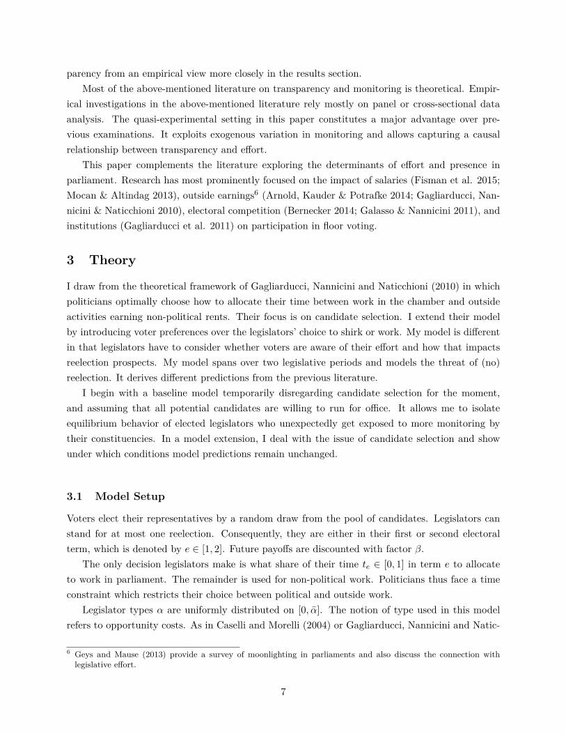
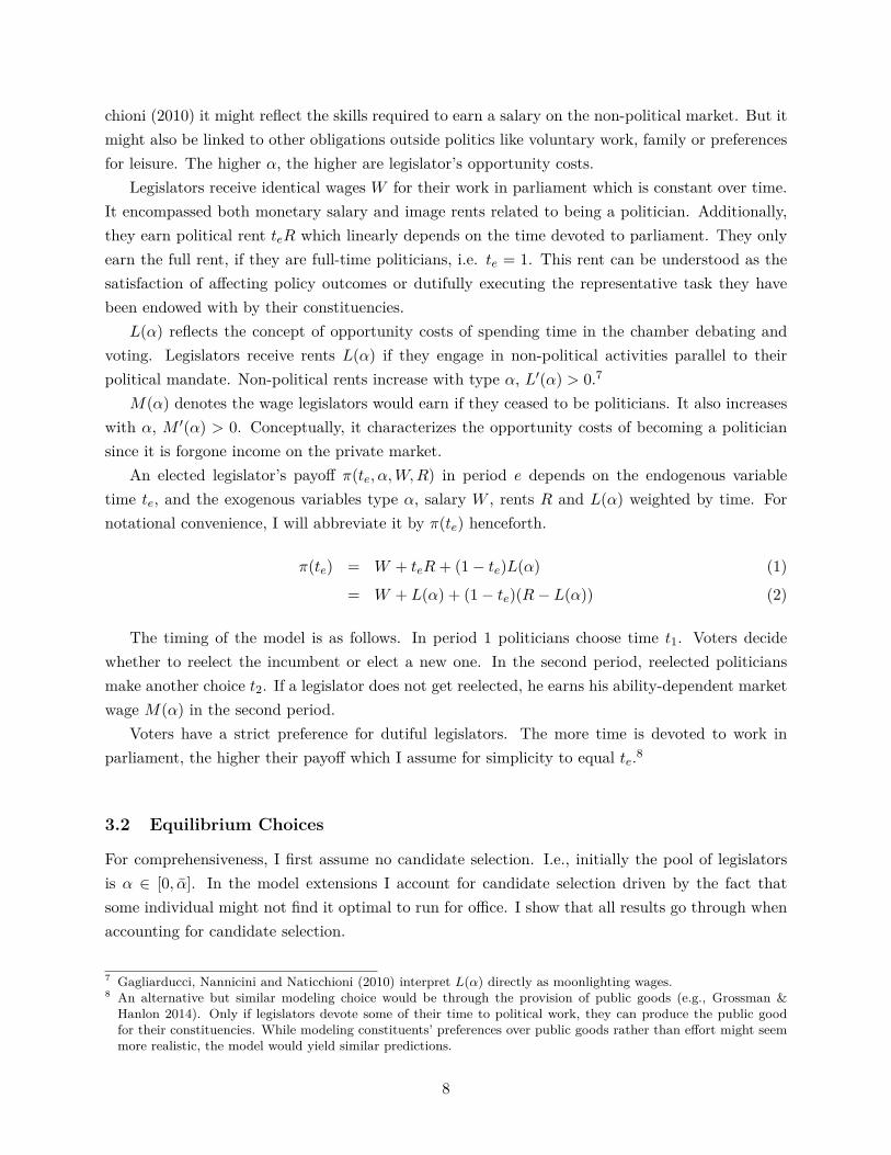
Figure 2 depicts an example of equilibrium choices with monitoring. While the lower and uppertails of the type distribution remain unchanged in comparison to the case without monitoring,types between [α, α] work during their first term and shirk in the second one. Suppose α = 0.6and α = 0.7, such that equation (8) is fulfilled and the share of working H-types is relatively low.In contrast, when α = 0.2 as in Figure 3, it is too likely that first-period workers will shirk in thesecond period. Then nobody gets reelected and legislators behave as without monitoring.

I now derive testable predictions from the model. Suppose that monitoring improves fromno monitoring to perfect monitoring during an ongoing term. L-types (α ∈ [0, α)) will continue

13The reelection mechanism is similar to the one in Besley (2004). Voters observe politicians implementing theirdesired policy but are uncertain over whether they will continue doing so in the second term.

12

FIG. 2: Equilibrium with Monitoring

0 α α

Work

R > L(α)

Shirk

R < L(α)α

t1 = 1t2 = 0

Note: Types α are distributed between 0 and α = 1. All types below α = 0.6 have low opportunity costs of voting(L(α) < R) and work. All types above α = 0.7 have high opportunity costs of voting (L(α) ≥ R) and thus shirk.Types between α and α work in the first period (t1 = 1) but shirk in the second one (t2 = 0). The reelection conditionαα> α

αis fulfilled since 0.6

0.7 >0.71 .

working and and legislators in the upper end of the distribution (α ∈ [α, α]) will continue shirking.All legislators in their second term will not adapt their behavior as well. If condition (8) holdsand the share of L-types in the population is relatively large such that working is rewarded withreelection, it will be optimal for H-type legislators α ∈ [α, α) in their first term to switch fromshirking to working. Averaging over all legislators, the expectation is that legislators will behavemore dutifully on average.

Prediction 1 If monitoring improves during an ongoing legislative period, absences will decreaseon average.

The average reduction in shirking is a consequence of some H-types adjusting their effort duringtheir fist term in order to please their voters. The main effect would therefore be expected in thesubgroup of incumbents running for reelection. In contrast, politicians ending their political careersdo not face reelection concerns and should not be affected by the change in monitoring. This isstated in the following prediction.

Prediction 2 If monitoring improves during an ongoing legislative period, absences will decreaseon average among politicians running for reelection. No change is expected for legislators in theirlast term.

This prediction can be generalized even more. Legislators who are particularly reliant on reelec-tion can be expected to be more responsive to monitoring than legislators who have less to loose ifnot reelected.

FIG. 3: Voters Do Not Reelect Working Incumbents

0 α αα

Note: Types α are distributed between 0 and α = 1. α = 0.2 and α = 0.7. The reelection condition αα> α

αis not

fulfilled since 0.20.7 <

0.71 .

13

3.3 Extension: Candidate Selection

The question is whether all politicians will find it optimal to become politicians in the first place.The empirically relevant case is the change in behavior when monitoring increases during an ongoinglegislative term. Therefore, I concentrate on candidate selection when monitoring is not available.I only have to distinguish L-types (α ∈ [0, α), who always work) from H-types (α ∈ [α, α], whoalways shirk).

To candidate, a legislator has to be better off being a politician than earning market wages.L-types candidate if W +R ≥M(α). Denote the type for which the condition holds with equalityby αL = M−1(W + R). Types above αL do not want to become politicians, whereas types belowthe threshold do. If 0 < αL < α, some L-types candidate; if αL < 0, nobody candidates; and ifαL > α, everybody candidates.

H-types candidate if W + L(α) ≥ M(α). If the condition holds (does not hold) for all types,everybody (nobody) becomes a politician. Maximizing the condition, allows to capture the interme-diate cases and arrive at the candidate selection result of Gagliarducci, Nannicini and Naticchioni(2010). If wages deteriorate when becoming a politician, L′(α) < M ′(α), negative hierarchicalsorting occurs and H-types with low α candidate. The opposite is true if earnings improve due tobecoming a politician, L′(α) > M ′(α).footnoteDiermeier, Keane and Merlo (2005) provide evidencefor such an earnings pattern in US Congress.

In order so sustain the model predictions and find an effect of monitoring on legislators’ effort,the existence of some H-types who are willing to mimic low α types in the first period, is required.Monitoring only has an effect if voters are uncertain over the legislators’ types even though theirbehavior can be observed. This is the case if either everybody becomes a politician, there is negativesorting (lower end of α distribution, or positive sorting with some working H-types running for office.

In sum, this extension provides the intuition that even when accounting for candidate selection,monitoring can have the expected effect derived from the main model.

3.4 Discussion

I briefly review and discuss some of the outcomes and modeling choices.The literature portrays a dark picture of politicians. Essentially voters are facing a trade-off

between diligent but incompetent representatives and able but shirking ones. Adding monitoringand the reelection rationale to the framework, slightly brightens the picture. Not only is it possiblethat high α types candidate for public appointment. Monitoring motivates part of them to exertmore effort. Extending the time horizon to a second period allows some high α types to committhemselves to work in the way preferred by voters if they get reelected for that.

If the ability to earn rents on the private market is correlated with political skills to, e.g., providepublic goods at a low cost, monitoring can improve the public goods provision. On the other hand,α may not only reflect wage-earning ability and competence, but the more general concept ofopportunity costs of doing politics. Electing low-α politicians then means selecting representatives

14

who are able to fully concentrate on their duties in parliament and not being distracted by othercompeting activities.

To keep with the literature, the punishment mechanism in the model is chosen to run via votersnot reelecting shirking politicians. Alternative punishment mechanisms through parties or interestgroups in the form of government functions or reduced campaign contributions would lead to thesame model predictions if they depended on (not) observing attendance.

4 Institutional Background and Descriptives

4.1 The Swiss Upper House

Switzerland has a bi-cameral parliamentary setup. The Lower House, the Nationalrat, is electedthrough a proportional system. The Upper House, the Ständerat, represents the Swiss cantons andis elected mostly through majoritarian elections. The two exceptions with proportional electionsare the cantons of Neuchâtel and Jura. Each of the 20 full cantons is represented by two legislators,and the six half-cantons hold one seat each. This adds up to 46 council members. The institutionalsetup closely resembles the one of the U.S. congress. The US Senate has many institutional analogiesto the Swiss Upper House. For more details on the Swiss political system, I refer the reader toKriesi and Trechsel (2008).

Importantly for this paper, the Swiss Parliament is traditionally viewed as a militia assembly.The original idea rests on the notion than citizens should engage themselves in politics or voluntaryactivities on top of their bread-earning work. Though both chambers have undergone significantprofessionalisation in the past decades (e.g., Müller 2015), the option to follow a salary-earningprofession next to holding a seat in parliament still exists and is made use off.

The focus of this paper is on the Upper House. It meets four times per year during pre-assigneddates in the spring, summer, fall and winter sessions. Each of the four yearly legislative sessionslasts three weeks. Meetings take place from Mondays to Thursdays. Monday meetings begin inthe afternoon allowing for same-day arrival from each part of Switzerland. Most of the remainingmeetings take place in the morning, though sometimes two meetings a day are scheduled. Finalpassage votes are decided upon almost exclusively on the very last Friday of a legislative session.This results in at least 13 and at most 15 meetings per legislative session. The legislative periodlasts for four years and commences with a winter session.

The 46 members of the Upper House who were elected in fall 2011 were born on average in 1956,the oldest member being born in 1945 and the youngest in 1979. Only roughly 20% are female andthe majority of 74% has German as their official language.14 22% hold a doctoral degree which issignificantly above the Swiss average of 5.6%.15 About a third have an officer rank in the Swissarmy. 72% are married and have 2 children on average. These are lower bounds since disclosure of14Note that legislators in the Upper House speak German, French and Italian. While the first two dominate, duringdebates legislators typically speak in their preferred language.

15The number was received on request from the Swiss Statistical Office and reflects the status quo in 2014.

15

marital status and number of children is not mandatory. 8.7% are elected through a proportionalsystem, the remainder is elected proportionally. At the beginning of the 49th legislative period,they have served 8 years in parliament or an equivalent of two terms. 20% are in their first term.Three quarters were running for reelection in the 2015 national elections, 12 retired afterwards.

More than two thirds of the members hold an occupation alongside their political mandatewhich I will refer to as moonlighting. However, already the four three-week sessions require timeimplying additional work load. On top, most councilors are members of specialized committees.Parallel careers with executive positions in the private sectors are therefore virtually impossible.16

The most commonly encountered professions among moonlighting politicians are lawyers (32.4%)and entrepreneurs (17.6%). Only roughly a third are full-time politicians.

Table 1 summarizes the descriptives. Personal information come from the parliament’s webpage.

Table 1: Descriptive Statistics of Individual Legisla-tors

Variable Mean Std. Dev Min. Max. Obs.

Birthyear 1956 7.464 1945 1979 46Female 0.196 0.401 0 1 46German 0.739 0.444 0 1 46Doctor 0.217 0.417 0 1 46Officer 0.348 0.482 0 1 46Married 0.717 0.455 0 1 46Children 2.0 1.530 0 6 46Proportional election 0.087 0.285 0 1 46Years in parliament 7.891 6.061 0 25.5 46First term 0.196 0.401 0 1 46Full-time politician 0.283 0.455 0 1 46Running for reelection 0.75 0.438 0 1 44

Note: Descriptive statistics. Characteristics of the 46 membersof the Upper House at the beginning of the 49th legislative periodin 2011. Source: Parliament homepage www.parlament.ch.

4.2 Institutional Change: Increase of Transparency

Traditionally, the Upper House has voted by show of hands. The president announced the votingalternatives and legislators raised their hands for their preferred alternative. Two designated mem-bers of the council served as vote counters. The aggregate voting outcome was documented in thechamber’s minutes. Since 2006 all sessions were recorded on video and are accessible online. Otherthan through the laborious screening of video records it was impossible to systematically monitorindividual legislators’ attendance and voting decisions.

The voting system was reformed to a more transparent one after a long and heated debate.

16The information is based on an interview with a current member of the Upper House conducted on 23 August,2016.

16

Though initially rejected by the majority of council members, the transparency bill17 was resumedafter counting mistakes were prominently detected by the media in winter 2012. It can thus beargued that the transparency bill was revived by an exogenous shock through media pressure.While the councilors generally agreed that a reduction in counting mistakes was desirable, concernswere voiced over the potential deterioration of discourse culture in the chamber. Increased pressurefrom the parties and the media were typically mentioned as arguments against publishing votingrecords. According to members of the Upper House, the partial publication of voting results wasthe result of a (very Swiss) compromise. The new voting system was approved with a majority of28 to 14 votes in spring 2013 and inaugurated one year later.

Starting in spring 2014, all votes in the Upper House are taken electronically. The system isoperationalized by a set of three buttons at every legislator’s desk. Each vote lasts for 30 secondsduring which vote choices can be adjusted flexibly. A flashing note on two clearly visible electronicboards signals the last eight seconds of the vote. The boards display a seating chart of the chamberand vote choices (green for yes, red for no, white for abstain) appear in real time. In cases of clearvoting majorities, it is common practice for chamber presidents to expedite the voting process.However, the last eight seconds of the vote are always visible and cannot be skipped.

While all votes are conducted electronically, individual decisions on four types of votes getpublished automatically on the parliament’s website in PDF format: a) final passage votes (ultimatedecision on acceptance/rejection of bill); b) total votes (votes taking place after several paragraph-by-paragraph votes before the bill is transferred to the Lower House); c) debt brakes (required forone-time expenses above CHF 20 million or recurring expenses above CHF 2 million); d) emergencyvotes (bills requiring immediate implementation). The PDF displays information on how eachindividual legislator votes (yes, no, abstain) and whether he was excused or did not participate inthe vote. It is also marked who acted as the chamber’s president. For the remainder of the paper,I will refer to vote types a) to d) as nominal votes, independent of the voting system at place. Theremaining votes, encompassing detail votes and procedural votes, remain unpublished. I will referto these types of votes as secret votes.18 The distinction of secret and nominal thus refers to thefact whether a type of vote is automatically published or not at some point in time.

The Swiss Lower House (Nationalrat) serves as a good example that changes in voting pro-cedures can transmit into public information on attendance rates. The Lower House takes allvotes electronically such that they are recorded and fully published online since 2007. Not onlyin theory, it is therefore easy to compute attendance rates for this chamber. Several newspapers,mostly tabloids with high circulation but also well-renowned newspapers, reported extensively onlegislators’ participatory shirking (e.g., 20 Minuten 2012a, 2012b; Neue Zürcher Zeitung 2014; SRF2012). They published rankings of the least dutifully acting legislators. Missing votes was exclu-sively framed as “bad” behavior. On top of newspaper articles, the independent policy platform

17The bill was the parliamentary initiative with bill number 11.490 by This Jenny 2011. All debates can be found in theparliament’s minutes, the Amtliches Bulletin (Parlamentsdienste) which are available online (www.parlament.ch).

18As before 2014, ten members of the Upper House suffice to request a recorded vote on any type of vote. However,legislators hardly ever make use of this option.

17

Politnetz offers rankings of attendance rates computed from nominal votes. It has started publish-ing this information for the Upper House precisely since the introduction of electronic voting.

4.3 Dataset and Measuring Absences

Absence during votes can take one of two forms: excused missing of a complete voting day orselective absence during some votes.

Excused absences are controlled daily by call of names at the beginning of each meeting (Stand-ing Orders of the Council of States 2015). Preferably, legislators should inform the House’s secretaryabout their absence in advance if possible. Excused members miss a complete meeting and con-sequently all votes taken on a particular day. The three recorded reasons for excused absenceare “illness”, “maternity leave”, and “other”. The residual category “other” encompasses absencesdue to commission work or travel abroad among others but cannot be directly attributed to morespecific causes.

Selective absences describe the cases when legislators fail to appear for a vote even though theywere present during the morning call of names. During the meetings, legislators are free to leavethe chamber at any point in time. Predominantly, they make use of this possibility to work, or formeetings with interest groups and lobbies. Other less frequent activities include private meetings,appointments with voters, school classes or simply taking a break.19 The chamber of the UpperHouse has two symmetric exits on the sides. They lead into antechambers equipped with tables andworking stations. When a vote is about to take place, a bell activated by the chamber president orthe secretary signals the legislators to return to the chamber. It is only audible in the antechambers.If councilors spend their time in the parliament’s cafe, they can follow the meetings on TV screenswhich, however, are not equipped with a sound system.20 The bell cannot be heard in other parts ofthe parliament building. In theory councilors have the opportunity to get back in time for votes.21

The data span the 49th legislative period commencing with the summer session 2012 and endingwith the last session in September 2015. All sessions and meetings are chronologically reported bydate in the parliamentary minutes (Wortprotokoll, Amtliches Bulletin). They cover all speeches,debates, and importantly votes including their aggregate voting outcomes. The type of vote isdocumented as well, allowing to code whether a vote was a nominal or a secret one. During thelegislative period, two of 46 members left the chamber prematurely, either due to health-relatedreasons or appointment into government. They were replaced by two new members. Table 9 in theAppendix reports the names and dates of the replacements.

Until 2014, a camera captures the councilors during votes. The videos allow me to construct a

19This information is based on an interview with a members of Upper House conducted on 18 August, 2016.20Traditionally, a member of the government is the last to speak before a vote. Seeing such a speech on screen istherefore one, albeit imprecise, indicator for an approaching vote.

21Fisman et al. (2015) report that members of the European Parliament only signed the register in the morning tosecure the daily allowance and subsequently leave the parliament for the entire day. Such a behavior on a regularbasis is uncommon in Switzerland. Legislators would typically remain within reach of the chamber.

18

dataset of individual attendance per vote prior to electronic voting.22 The seating arrangement inthe chamber varies little over time, facilitating the tracking of legislators. Legislators are countedas present if they sit on their designated places during a vote. They are treated as absent if theyhave left the chamber.

Starting in 2014 when electronic voting was first introduced, the video recordings of all meetingscontinued to exist. The difference with regard to filming lies in the camera capturing one of theelectronic boards during the time of the vote instead of the legislators. I use the final votingoutcome displayed on the board to code whether a legislator attended a vote or not.23

I deal with two special cases relating to the coding of absences. The first one regards the chamberpresidents, the other one the pre-reform vote counters. The chamber presidents are elected membersof the Upper House. They guide through the meetings, make all announcements, and conduct thevotes during a term of one year. During that time they do not actively participate in votes with theexception of debt brakes, emergency votes, and ties between yes and no votes. They consequentlyvote rarely (though they are present), and the vast majority of their voting activity concentrateson nominal votes. I treat legislators acting as chamber presidents as being present for this reason.

Vote counters constitute another special case in the pre-reform period. Though they are visibleon video, it is typically unclear whether they have voted since they do not actively raise their hand.I code all vote counters as present. I will run robustness tests regarding the special role of chamberpresidents and vote counters since they have much less leeway to strategic absence due to theirprominent institutional roles requiring the continuous presence during meetings.

Data sources are the following. I received the complete video recordings of all meetings coveringthe full 49th legislative period from the parliamentary services. Information on excused memberscomes from the parliament’s official attendance registers. Causes of absences were provided by theparliament’s office.

4.4 Descriptives and Voting Patterns

The main descriptives at vote level and regarding individual absences are summarized in Table 2.The data encompass a total of 1,782 votes. It corresponds to about 15 votes per meeting. Around56% were secret votes, the remainder were nominal ones. Total votes (21%) and final passage votes(14%) are the most frequent nominal categories. Debt brakes and emergency votes account for8.5% and 0.2% of all votes respectively. Most votes are taken on Wednesdays and Thursdays (25%respectively). They are least frequent on Mondays and Tuesdays (17% respectively).

Votes take place between the first minute of the meeting and after more than 6 hours with an

22The video records of the Upper Council have been used to explore the quality of political representation andvoting patterns in this chamber (e.g., Benesch, Bütler & Hofer 2015; Bütikofer 2014; Eichenberger, Stadelmann &Portmann 2012; Hug & Martin 2011; Portmann & Stadelmann 2013; Stadelmann, Portmann & Eichenberger 2013,2014).

23 In theory it is possible that a legislator is physically present during a vote but does not press any of the votebuttons. I count such behavior as absence since the legislator did not actively participate in the vote. This is alsohow absence statistics would be constructed.

19

average of 2 hours. Though many votes appear as single, “independent” votes (48.5%), clustersof several votes in a row are just as frequent. I define a “block” as consecutive votes withoutinterruption by speeches or debates. There are on average 4.8 votes in such a block. Excludingfinal passage votes, which are characterized by very long blocks with up to 29 votes in a row, theaverage is 2 votes per block. An exemplary distribution of votes can be found in Figure 4. It showsthe occurrence of nominal votes (circles) and secret votes (diamonds) over time in minutes on arandomly picked day (29 May, 2012). 8 out of 14 votes were nominal. The first four votes areexecuted in a block one after the other. They are followed by six independent votes every 9 to 13minutes. The meeting finishes with four consecutive votes in a block.

Independent votes are most likely to be secret (81%) and total votes (16.5%). Vote blocks areeither exclusively made of secret votes (24%), nominal votes (29%) or a mix thereof (46%). In suchmixed blocks, secret votes make up the largest share (42.6%) and they almost always commence ablock. Purely nominal blocks are dominated by total votes (75.4%) and debt votes (22.9%).

All time variables have the potential to affect absences. In the regression analysis, I will controlfor the time a vote was taken during a meeting, the number of votes in a block and the votesposition in a block, as well as the day of the week.

Absences account for 12.5% of individual observations, i.e., legislators miss one in eight votes.On average, 5 legislators are absent during votes. 1.7% can be attributed to excused absences.The share of votes missed at individual level, however, varies tremendously. While some legislators

FIG. 4: Distribution of votes over time during a meeting

1580

1585

1590

1595

Vot

e ID

140 160 180 200 220Time in minutes

Note: Vote patterns on 29 May, 2012. Occurrence of nominal (circle) and secret (diamonds) votes. Thex-axis shows time in minutes (with 0 defined as the beginning of the meeting). The y-axis shows a continuousvote ID.

20

Table 2: Descriptive Statistics of Vote Characteris-tics

Variable Mean Std. Dev Min. Max. Obs.

Secret 0.558 0.497 0 1 1782Total vote 0.212 0.409 0 1 1782Final vote 0.143 0.350 0 1 1782Debt brake 0.085 0.279 0 1 1782Emergency vote 0.002 0.047 0 1 1782

Absent 0.125 0.331 0 1 54019Excused 0.017 0.131 0 1 54019

Time 2.043 1.406 0 6.4 1782Votes per block 4.669 6.667 1 29 1782Position in block 2.834 4.068 1 29 1782Monday 0.173 0.379 0 1 309Tuesday 0.171 0.377 0 1 305Wednesday 0.251 0.434 0 1 447Thursday 0.253 0.435 0 1 451Friday 0.152 0.359 0 1 270

Note: Descriptive statistics of vote characteristics. Source:Parliament homepage www.parlament.ch.; Amtliches Bulletin;Videos of legislative sessions 2012-2015.

miss as little as 3.3% of all votes, others are absent during up to 27% of the votes. This gives anintuition for the strong individual variation in attendance rates across legislators. Absences arehighest during total votes (15%) and slightly below 12% during debt and secret votes.

As I will argue below, total votes belong to the vote category best suitable for the analysis ofnominal votes. Final passage votes, in contrast, have institutional characteristics which make atreatment effect of monitoring unlikely.24

A stylized fact about procedures on the final session day is that almost exclusively final passagevotes are taken which are nominal votes by definition.25 These meetings last for less than an hourwith all final votes taken consecutively without interruptions: the average time between one finalvote and the next one amounts to 45 seconds (and the maximum time to 2 minutes), compared to22 minutes on average for votes taken on all other days. Excluding excused legislators, only 0.49%of 11,262 observations from last session days are absences. In other words, if a legislator is presenton the final session day, he is going to participate in all votes almost with certainty. This holdsalready for pre-reform votes, such that no treatment effect can be expected.

24 Indeed, running the baseline regressions with final passage votes as the only nominal category, yields no significantresult. It suggests that no changes in absences during final passage votes were induced after reform, even thoughmonitoring improved for these vote categories.

25The exception are 10 secret votes which took place on Fridays.

21

5 Identification

Prediction 1

The aim is to identify the average treatment effect on the treated of monitoring on shirking byabsence from floor voting. The idea is to compare individual attendance in the Upper Houseduring nominal and secret votes before and after the reform. The main model Prediction 1 tobe tested suggests a drop in the probability of being absent once absences are monitored. Thedependent variable of interest Absenceij takes on value 1 if legislator i was absent during vote j,and 0 if he was present.

Identification is based on the exogenous variation of the monitoring technology for some votes(nominal votes) while the remaining ones are always kept undisclosed (secret votes). Nominalvotes therefore define the treatment group, and are compared to the non-treated votes in thecontrol group. The variable Nominalij takes on value 1 if vote j was such a vote. It is 0 for allsecret votes. Control and treatment are thus defined over vote categories. The allocation intocontrol and treatment group is defined by the legal form of the vote. There is no concern about apotential selection into treatment bias. Moreover, since complete video recordings of all legislativesessions exist, the sample is not selective.26

The focus on a single legislative period ensures an almost identical composition of the cham-ber. The same individuals are observed voting on the two different kinds of votes before and afterthe treatment. By controlling for individual legislator fixed effects, I estimate the within varia-tion of absences while shutting out all time-invariant legislator characteristics. Examples of suchtime-invariant control variables frequently used in the voting literature are birth year, outside em-ployment, marital status, number of children or party affiliation. Including legislator fixed effectsallows to estimate the individual treatment for legislators instead of estimating variation betweenthe politicians.

The variable Reformij is defined as 1 for all votes taken after the change in voting procedures,and 0 before the reform. Since the institutional change takes place almost in the middle of thelegislative period, a large number of votes takes place before and after the reform for both types ofvotes.

Are published and never-published votes randomly distributed or does a selection issue exist? Ifa difference between the pre- and post-reform period existed, it might affect the results. I examinethe distribution of votes types over time (cf. Figure 5). The share of votes getting published variesstrongly day by day. But a t-test rejects the hypothesis that the share of publishable votes issystematically different before and after the change of the voting system. I also run a t-test of theshares of votes taken by type and do not find any significant difference between the numbers of

26Recorded votes might constitute a selective sample of the universe of votes (Carrubba, Gabel & Hug 2008; Carrubaet al. 2006; Hug 2010). The bias is particularly strong if recorded votes are conducted on request: members ofparliament are called to order by the mere appearance of a roll call vote and consequently are present more oftenduring recorded votes. The bias is less severe in countries like Italy where most votes are taken electronically (cf.description by Gagliarducci et al. 2010).

22

votes before and after electronic voting. The common support assumption demanding a sufficientnumber of observations in all subgroups defined by treatment and control is thus fulfilled.

The reform itself was exogenously driven by the medial revelation of result-critical countingmistakes. The transparency bill had originally been rejected and was only revived through mediapressure - a process uncommon to Swiss politics.

Following the above argumentation allows me to run a difference-in-difference (DiD) regression.Let α be the intercept, β1 to β3 the main coefficients, Xij a vector of control variables as explainedin the previous section and ξ its vector of coefficients, ui the legislator fixed effects with coefficientsψ, and εij the error term. The estimation equation is of the following form:

Absentij = α+ β1Nominalij ×Reformij + β2Nominalij + β3Reformij + ξXij + ψui + εij

(9)

The coefficient of interest β1 identifies the average treatment effect on the treated (ATET) underseveral assumptions I will detail below. From theory, I expect the coefficient to be negative,reflecting a decrease of the probability of being absent once attendance rates can be monitored

FIG. 5: Distribution of Nominal Votes per Day

0.0

5.1

.15

.2

0 .5 1 0 .5 1

0 1

Frac

tion

Share of Nominal Votes per DayGraphs by reform

Note: Distribution of the share of nominal votes per day conducted before (0) and after (1) the reform.

23

for nominal votes. β2 represents the pre-reform difference in absences between nominal and secretvotes. There is no theoretical expectation for this coefficient. β3 is the change in absence ratesfor secret votes around the reform. In theory, the reform should have no effect on absences duringsecret votes. However, factors unrelated to monitoring but changing over time might be at play,making the use of a control group necessary in the first place. For instance, approaching electionsmight motivate legislators to be present more often during all kinds of votes. Lower absence ratesin the second half of the legislative period might thus be an artifact of an electoral cycle and havelittle to do with improved monitoring. Also, bills differ in their characteristics which might varyover time in a non-random fashion. Some of these characteristics, e.g. importance or topic, mightbe driving absence rates in a way orthogonal to the monitoring change.

The most important assumption for running a DiD regression is a common trend betweennominal and secret votes:

Assumption 1 (Common trend conditional on covariates) If the voting system in the Up-per House had not changed, the difference in absences between nominal and secret votes, conditional

FIG. 6: Inspection of common trend assumption

-.06

-.03

0.0

3.0

6

0 Spring 2013 Spring 2014 Spring 2015Session

Nominal Secret

Note: The x-axis is a continuous indicator of voting sessions. The y-axis shows the aggregate residuals persession and type of vote of a regression of Absent on a set of covariates.

24

on covariates, would have evolved as before the reform.

Though the validity of this assumption cannot be investigated in full since it relies on potentialoutcomes, the development of pre-reform trends in the control and treatment groups can be exam-ined. I regress the dependent variable Absent on control variables Xij and legislator fixed effectsfor each of the four subgroups defined by the combinations of nominal/secret votes and pre/postreform. I then calculate the residuals and plot the mean residuals aggregated by voting session.

Figure 6 shows the development of the residual over time, the dashed line representing nominalvotes and the solid line secret votes. The vertical line marks the timing of the reform. Thedevelopment between control and treatment group evolves in parallel, especially in the first fourperiods. The gap slightly widens in summer 2013. The fall session 2013 is an extreme outlier.For robustness, I will drop this session in the empirical analysis. But it does not affect the overallresults. After the treatment, the gap between the residuals closes and remains close to zero. Insum, this provides some evidence that treatment and control group evolved in a similar fashion inthe pre-treatment period. It also gives guidance to carefully deal with the outlier.

The next assumption relates to the fact that not only the rules regarding the publication ofindividual voting decisions have changed, but also the procedure switched from voting by show ofhand to electronic voting. This change occurred for all types of votes.

Assumption 2 (Electronic Voting) If electronic voting had an effect on the probability of beingabsent, the pure “electronic voting effect” is identical for nominal and secret votes.

In theory, the electronic voting system might have made it easier to submit a valid vote: theelectronic buttons can be pressed at any point in time as long as the electronic system operates.In contrast, when votes were still takes by show of hands, the questions to vote “yes”, “no” or“abstain” were taken one after each other. For legislators planning to accept a bill, presence wasrequired already at the start of the vote. Such an effect can be expected irrespective of the votetype.

Prediction 2

The second model prediction to be tested postulates a zero effect for legislators in their last term,in contrast to a negative effect of monitoring on absences for legislators continuing their politicalcareers. The prediction requires a test of a differential treatment effect in two exogenously definedgroups. Let Groupij = 1 denote one such group, and Groupij = 0 the remaining legislators. Thevariable is kept intentionally general as I will use several groups in the empirical analysis.

I start with the above estimation equation (9) and interact its main elements with the Group

25

variable.

Absentij = α+ γ1Nominalij ×Reformij + γ2Nominalij ×Reformij ×Groupij+γ3Reformij ×Groupij + γ4Nominalij ×Groupij + γ5Nominalij

+γ6Reformij + γ7Groupij + ξXij + ψui + εij (10)

γ1 and γ2 are the two most relevant coefficients. γ1 is the marginal reform effect for the subgroupdefined by Groupij = 0. γ2 indicates whether the reform effect differs by subgroup. The sum ofthe coefficients γ1 + γ2 reflects the marginal reform effect for Groupij = 1.

I will test for difference between running and retiring legislators. The next distinction will bebetween full-time politicians and legislators engaging in moonlighting. The last distinction is by thenumber of interest groups. Both choices are directly motivated by the model in which opportunitycosts of floor voting and the value of reelection play a role.

26

6 Results

6.1 Main Results

All regressions are run with ordinary least squares.27. Standard errors are clustered at legislatorlevel because treatment is at individual level and standard errors are most likely correlated atindividual level. With 46 legislators in the Upper House, the number of clusters is sufficiently high(Cameron, Gelbach & Miller 2008).

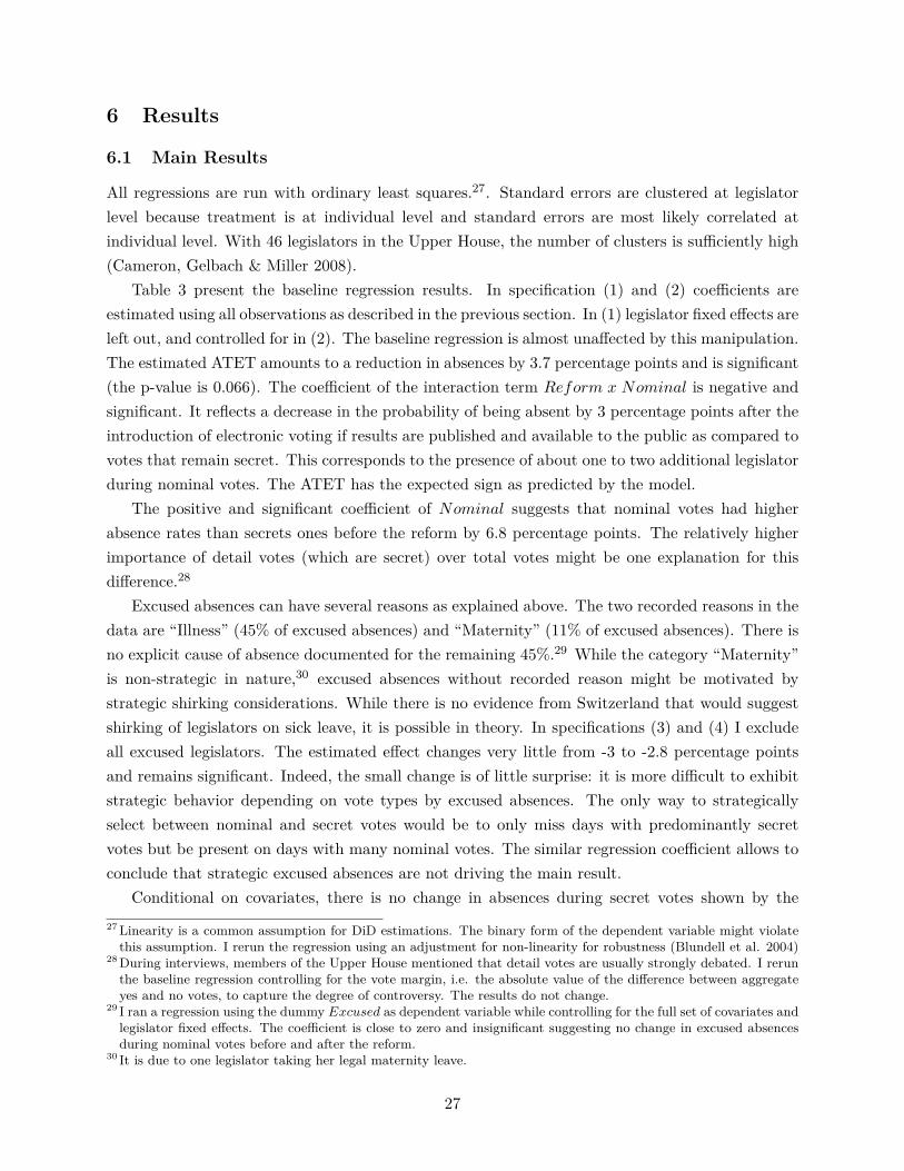
Table 3 present the baseline regression results. In specification (1) and (2) coefficients areestimated using all observations as described in the previous section. In (1) legislator fixed effects areleft out, and controlled for in (2). The baseline regression is almost unaffected by this manipulation.The estimated ATET amounts to a reduction in absences by 3.7 percentage points and is significant(the p-value is 0.066). The coefficient of the interaction term Reform x Nominal is negative andsignificant. It reflects a decrease in the probability of being absent by 3 percentage points after theintroduction of electronic voting if results are published and available to the public as compared tovotes that remain secret. This corresponds to the presence of about one to two additional legislatorduring nominal votes. The ATET has the expected sign as predicted by the model.

The positive and significant coefficient of Nominal suggests that nominal votes had higherabsence rates than secrets ones before the reform by 6.8 percentage points. The relatively higherimportance of detail votes (which are secret) over total votes might be one explanation for thisdifference.28

Excused absences can have several reasons as explained above. The two recorded reasons in thedata are “Illness” (45% of excused absences) and “Maternity” (11% of excused absences). There isno explicit cause of absence documented for the remaining 45%.29 While the category “Maternity”is non-strategic in nature,30 excused absences without recorded reason might be motivated bystrategic shirking considerations. While there is no evidence from Switzerland that would suggestshirking of legislators on sick leave, it is possible in theory. In specifications (3) and (4) I excludeall excused legislators. The estimated effect changes very little from -3 to -2.8 percentage pointsand remains significant. Indeed, the small change is of little surprise: it is more difficult to exhibitstrategic behavior depending on vote types by excused absences. The only way to strategicallyselect between nominal and secret votes would be to only miss days with predominantly secretvotes but be present on days with many nominal votes. The similar regression coefficient allows toconclude that strategic excused absences are not driving the main result.

Conditional on covariates, there is no change in absences during secret votes shown by the27Linearity is a common assumption for DiD estimations. The binary form of the dependent variable might violatethis assumption. I rerun the regression using an adjustment for non-linearity for robustness (Blundell et al. 2004)

28During interviews, members of the Upper House mentioned that detail votes are usually strongly debated. I rerunthe baseline regression controlling for the vote margin, i.e. the absolute value of the difference between aggregateyes and no votes, to capture the degree of controversy. The results do not change.

29 I ran a regression using the dummy Excused as dependent variable while controlling for the full set of covariates andlegislator fixed effects. The coefficient is close to zero and insignificant suggesting no change in excused absencesduring nominal votes before and after the reform.

30 It is due to one legislator taking her legal maternity leave.

27

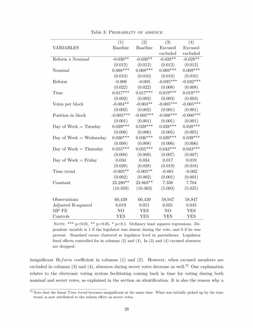
Table 3: Probability of absence

(1) (2) (3) (4)VARIABLES Baseline Baseline Excused Excused

excluded excludedReform x Nominal -0.030** -0.030** -0.028** -0.028**

(0.012) (0.012) (0.012) (0.012)Nominal 0.068*** 0.068*** 0.069*** 0.069***

(0.010) (0.010) (0.010) (0.010)Reform -0.008 -0.005 -0.035*** -0.032***

(0.022) (0.022) (0.008) (0.008)Time 0.017*** 0.017*** 0.019*** 0.019***

(0.002) (0.002) (0.003) (0.003)Votes per block -0.004** -0.004** -0.005*** -0.005***

(0.002) (0.002) (0.001) (0.001)Position in block -0.005*** -0.005*** -0.006*** -0.006***

(0.001) (0.001) (0.001) (0.001)Day of Week = Tuesday 0.029*** 0.029*** 0.028*** 0.028***

(0.006) (0.006) (0.005) (0.005)Day of Week = Wednesday 0.036*** 0.036*** 0.039*** 0.039***

(0.008) (0.008) (0.006) (0.006)Day of Week = Thursday 0.055*** 0.055*** 0.043*** 0.043***

(0.009) (0.009) (0.007) (0.007)Day of Week = Friday 0.034 0.034 0.017 0.019

(0.028) (0.028) (0.019) (0.018)Time trend -0.005** -0.005** -0.001 -0.002

(0.002) (0.002) (0.001) (0.001)Constant 23.280** 23.863** 7.338 7.704

(10.359) (10.363) (5.003) (5.025)

Observations 60,439 60,439 58,947 58,947Adjusted R-squared 0.019 0.051 0.021 0.045MP FE NO YES NO YESControls YES YES YES YESNote: *** p<0.01, ** p<0.05, * p<0.1. Ordinary least squares regressions. De-pendent variable is 1 if the legislator was absent during the vote, and 0 if he waspresent. Standard errors clustered at legislator level in parentheses. Legislatorfixed effects controlled for in columns (2) and (4). In (3) and (4) excused absencesare dropped.

insignificant Reform coefficient in columns (1) and (2). However, when excused members areexcluded in columns (3) and (4), absences during secret votes decrease as well.31 One explanationrelates to the electronic voting system facilitating coming back in time for voting during bothnominal and secret votes, as explained in the section on identification. It is also the reason why a

31Note that the linear T ime trend becomes insignificant at the same time. What was initially picked up by the timetrend, is now attributed to the reform effect on secret votes.

28

control group is necessary in the empirical setting. This intuition was confirmed in interviews withmembers of the Upper House.

The signs of the control variables can be explained intuitively. The larger Time, i.e., the longera meeting takes, the more legislators leave the chamber. Absences become less likely if more votestake place during a voting block. Similarly, the later a vote takes place during a voting block, thelower the absence rates. Though the coefficients are small in absolute terms, they go well with theinterpretation that if many votes take place after each other, legislators are more likely to finallyreturn to the chamber. On all days of the week absences are higher than on Mondays. The furtheralong the week, the more absences can be witnessed. The linear session time trend is negative andsignificant in columns (1) and (2) suggesting a reduction in absences over time.32

6.2 Robustness

Table 4 shows the results of a set of robustness checks. Legislator fixed effects and covariates arealways controlled for.

The data panel is largely balanced due to concentrating on a single legislative period. There arethree reasons why the panel is not perfectly balanced. I will explain each one of them and providea robustness check. First, pre-reform data are based on observing presence during votes on video.While the quality of the records is generally good, the videos suffer from some imperfections.Sometimes the camera does not capture the entire chamber. In many cases the chamber’s vicepresident, who’s seat is located in the front, is omitted on the records. In total, 1% of pre-reformobservations is missing, though there is no imbalance in missing between secret and nominal votes.In contrast, post-reform data have no missing observations by definition since the camera alwayscaptures the electronic board in full. The missing observations can be almost fully attributed to thetwo legislators acting as vice presidents in 2012 and 2013 because the camera captures them seldom.Dropping all observations from these two councilors in column (1) produces a similar coefficient asbefore (-0.027) which stays significant though at a lower level.33

Second, chamber presidents and counters have special duties and have - almost by definition -lower absence rates than their peers during this time. During their presidencies and time as votecounters, these legislators’ presence during vote is not based on strategic considerations. In column(2) I therefore drop all observations from legislators acting as either presidents or vote counters.The regression coefficient is almost unaffected by this reduction in the sample and gets even slightlymore negative (-0.031) .

Third, two legislators dropped out from the Upper House before the reform.34 Their substitutesreplaced them after the reform. They consequently lack either pre- or post-reform observations.

32Lindstädt and Vander Wielen (2011) show with US data that legislators moderate their policies before electionsdue to a peek in media attention. However, they vote more extremely once monitoring wanes.

33Even when dropping all eight legislators for whom observations are incomplete yields a significantly negative effect(-0.037).

34One legislator passed away in 2013. The other one stepped down due to deteriorating health.

29

Though the replacements are members of the same parties and come from the identical canton,they might react differently to monitoring. I drop the four legislators in question in column (3).The main coefficient changes only slightly to -0.029.

The occurrence of voting blocks has already been discussed: while some votes take place inde-pendently after a round of debates, other votes are taken in a “block” one after the other. Theblocks might consist of exclusively of nominal or secret votes: 72% of blocks in the sample consistof secret votes only, and 19 % of nominal votes only. The remainder of 9% contains both nominaland secret votes. Since absences in voting blocks are correlated, spill-over effects from one type ofvote to the other within the same block are possible in theory. E.g., lower post-reform absencesduring nominal votes might decrease absences during secret ones if the two types of votes are takenone after the other. This would bias the DiD coefficient towards zero. A possible test is to run theregressions based on a sample of voting blocks containing either secret votes or nominal ones, butnot the two of them. In column (4) I drop the 9% of mixed blocks reducing the sample to below50,000. The coefficient becomes even more negative (-0.04) and stays significant. Potentially, theabove-described spill-over mechanisms were at play and have led to a too small coefficient.

In theory it is possible that electronic voting affects the way bills are proposed such that billsbeing discussed differ systematically before and after the reform. Similarly to Benesch, Bütler andHofer (2015) I restrict my sample to bills that have been started before the reform in 2014 anddrop 348 votes from post-reform bills. This reduces the sample size and disregards a seizable shareof post-reform observations. Regardless of this manipulation, the main coefficient in column (5) isnegative and significant. Its size is changed to -0.024.

30

Table 4: Probability of absence - Robustness

(1) (2) (3) (4) (5)VARIABLES Missings Presidents New members Blocks Old Bills

dropped excluded excludedReform x Nominal -0.027* -0.031** -0.029** -0.040** -0.024**

(0.014) (0.013) (0.012) (0.015) (0.011)Nominal 0.066*** 0.074*** 0.067*** 0.089*** 0.065***

(0.010) (0.010) (0.010) (0.013) (0.010)Reform -0.005 -0.006 -0.006 -0.005 -0.004

(0.027) (0.024) (0.022) (0.023) (0.024)Constant 27.947** 27.871** 23.315** 24.208** 26.265**

(12.754) (11.007) (10.426) (10.492) (11.241)

Observations 47,464 55,409 58,018 49,939 44,457Adjusted R-squared 0.057 0.052 0.050 0.055 0.053MP FE YES YES YES YES YESControls YES YES YES YES YESNote: *** p<0.01, ** p<0.05, * p<0.1. Ordinary least squares regressions. Dependentvariable is 1 if the legislator was absent during the vote, and 0 if he was present. Standarderrors clustered at legislator level in parentheses. Legislator fixed effects and covariates arealways controlled for. In (1) all observations from legislators with missing observations areexcluded. In (2) all observations from presidents and vote counters are excluded. In (3) allobservations from two substitute legislators are dropped. In (4) voting blocks including bothsecret and nominal votes are excluded. In (5) only bills started before 2014 are included.

31

6.3 Heterogeneous Effects

In this section, I analyze differential effects for groups of legislators potentially differently affected bymonitoring. The mechanism at work runs through reelection prospects. Some groups of legislatorsare more dependent on getting elected for another terms while others have alternative opportunities.Three subgroups are distinguished. First, from the model differential effects can be expecteddepending on whether legislators were candidates in the 2015 election or decided to retire. Next,full-time politicians and legislators with an outside occupation in the private sector are checked fordifferences. While the former are reliant on getting reelected, moonlighters might have alternativecareers. Last, the number of interest groups of a legislator is taken into account. While interestgroups take time to deal with, they might be valuable in case the political career is terminated.

6.3.1 Running for Reelection

The literature documents differential behavior of legislators contained by reelection prospects.There is (partial) evidence for more shirking towards the end of the political career by votingagainst constituencies’ interests and (robust) evidence for reducing presence in parliament (e.g.,Lott 1990; Rothenberg & Sanders 2000).

Model Prediction 2 suggests that better monitoring should affect incumbents running for reelec-tion and those in their last term differently. Politicians aiming at continuing their political careershave to cater to their voters’ interests. Legislators not facing reelection constraints, in contrast,should be less susceptible to monitoring.

The expectation thus is that the change in the voting procedures should have a stronger effecton legislators standing for reelection than on legislators terminating their political careers at theend of the legislative period. In total 34 members of the Upper House were candidates for the nextelection, whereas 12 decided to step down.

Retirement can take two forms: voluntary or in anticipation of a potential defeat at the ap-proaching elections. Some legislators devote their lives to political work, while others utilize politicaloffices as stepping stones for non-political careers.35,36 In the case of the Swiss Upper House thenotion of career politicians seems to dominate. Office-holders not running in the 2015 election werebetween 63 and 70 years old in 2015. On average, they were ten years older than legislators runningfor the next term. This suggests that legislators are more likely going into voluntary retirement.However, an often used argument in the literature states that legislators anticipating electoral de-feat are more likely to retire. Or if legislators retired because they disliked transparency this wouldaffect the estimates. For robustness, I therefore use age in 2015 as an instrument for retirement.

The variableRetiring takes on value 0 if a legislator stood for reelection in 2015, and 1 otherwise.It is interacted with the standard DiD estimation equation such that a heterogeneous effect between

35Mattozzi and Merlo (2008) make this distinction between what they call “career politicians” and individuals with“political careers”.

36E.g., Diermeier, Keane and Merlo (2005) for the US Congress.

32

candidates and retiring legislators can be tested for. Observations from the two members leavingthe Upper House before 2014 are dropped because there is no retirement decision involved.

Comparing pre-reform absences among the two groups, no significant difference can be found:both miss around 14% of secret and 19% of nominal votes on average. Table 5 shows the regressionresults. I first repeat the baseline regression with the reduced sample to ensure that sample selectiondoes not affect the results. As column (1) shows, dropping the two legislators has little effect onthe main coefficient (-0.028).

Column (2) shows the estimation with heterogeneous effects. The coefficient of the DiD in-teraction Reform x Nominal can be interpreted as the reform effect for legislators running forreelection (Retiring = 0). It is significantly negative: incumbents standing for the 2015 electionreduce their absences during nominal votes by 4.2 percentage points. The effect is considerablylarger (i.e., more negative) than the baseline effect of -2.8 percentage points in the pooled samplein column (1). It is therefore the subsample of politicians exposed to the threat of (no) reelectionwho drive the average result.

The coefficient of the triple interaction has a negative and significant value. It means thatlegislators standing for reelection reduce their absences during nominal votes by 5.5 percentagepoints more than legislators retiring. The marginal reform effect for retiring politicians is the sumof the coefficients of the triple interaction and the DiD effect. It is not significantly different fromzero, indicating no effect of the reform on retiring politicians (results in the Appendix).

The results are robust to the exclusion of observations from the two new members who enteredthe Upper House as substitutes in 2014. This not only balances the panel but also drops twomembers who could have been expected to stand for reelection (in fact, they both did). The resultsare in column (3). In column (4) I exclude observations from excused absences. The marginalreform effect for candidates remains significant and is of similar size as before (-0.037). In column(5) retirement is instrumented with age which is an exogenous variable. All interactions withretirement are instrumented by interactions of the same variable with age. Results change verylittle and are thus not driven by the endogeneity of the retirement decision.

The results are in line with the theoretical expectation that politicians facing reelection con-straints are more susceptible to monitoring. In contrast, legislators who end their political careerare not concerned with punishment by their constituencies. The result thus confirms the modelprediction that legislators in their last term behave like lame ducks and do not react to incentivesrelated to reelection prospects.

33

Table 5: Heterogeneous Effects: Running for Reelection

(1) (2) (3) (4) (5)VARIABLES Baseline All New members Excused IV

excluded excludedReform x Nominal -0.028** -0.042*** -0.043*** -0.037** -0.030***

(0.012) (0.014) (0.013) (0.014) (0.008)Retiring x Reform x Nominal 0.055** 0.057** 0.046* 0.036*

(0.027) (0.027) (0.023) (0.022)Retiring x Reform -0.002 -0.003 -0.007 -0.017

(0.021) (0.021) (0.017) (0.013)Retiring x Nominal -0.009 -0.009 -0.012 0.022

(0.024) (0.024) (0.019) (0.016)Reform -0.004 -0.003 -0.006 -0.031*** 0.001

(0.022) (0.023) (0.023) (0.009) (0.007)Nominal 0.066*** 0.069*** 0.069*** 0.070*** 0.047***

(0.010) (0.012) (0.012) (0.012) (0.006)Retiring 0.025* 0.099*** 0.025* 0.005

(0.014) (0.011) (0.013) (0.080)

Observations 59,252 59,252 58,018 57,781 59,252Adjusted R-squared 0.050 0.050 0.050 0.043 0.050MP FE YES YES YES YES YESControls YES YES YES YES YESNote: *** p<0.01, ** p<0.05, * p<0.1. Ordinary least squares regressions. Dependent variable is 1if the legislator was absent during the vote, and 0 if he was present. Retired is 1 if the legislator doesnot run for reelection in 2015, and 0 else. Standard errors clustered at legislator level in parentheses.Two legislators leaving the Upper House before 2014 are excluded. Legislator fixed effects and covari-ates are always controlled for. (1) repeats the baseline regression. In (2) heterogeneous effects areestimated. In (3) all observations from two substitute legislators are dropped. In (4) excused absencesare dropped. (5) shows an IV regression using Age in 2015 as instrument for retirement from politics.

34

6.3.2 Moonlighters and Full-Time Politicians

All legislators have to provide information about their outside occupation. 14 original membersof the Upper House and one substitute are full-time politicians. They are classified accordingto official documentations and information on their personal websites. The information has beenconfirmed through interviews with legislators.37

Before the reform full-time politicians miss around 13% of all nominal votes on average. This issignificantly less than the 21% among moonlighting legislators. During secret pre-reform votes thetrend is similar: moonlighters miss about 16% of all votes in contrast to 9% by full-time politicians.Without monitoring, full-time politicians put more time into voting than politicians with outsideoccupation. It goes well with the notion that some legislators have dedicated their careers to politicsand thus put more effort into floor voting.38

The marginal reform effect for full-time politicians is negative and significant (column 1): full-time legislators reduce their absences during nominal votes significantly by 5.1 percentage points.The triple-interaction coefficient is positive though insignificant. Testing for the marginal reformeffect in the subgroup of moonlighting politicians reveals no significant impact of monitoring onthis subgroup.

Dropping the two newest members (column 2), or dropping all excused absences (column 3)yields an even more negative treatment effect among career politicians. The triple interactionbecomes significant in column (2), suggesting a difference in the marginal reform effect betweenfull-time politicians and moonlighters: politicians with outside occupations do not change theirabsences during nominal relative to secret votes.

The finding adds interesting insights about the behavior of legislators depending on their outsideoptions. Incumbents who have dedicated their lives to political careers, depend more strongly onreelection. Serving in the Upper House has become their main profession and alternative careersoutside politics are not immediately available. This is a potential interpretation of why careerpoliticians not only shirk less a priori but also react more strongly to monitoring. Moonlightingpoliticians, however, have an outside occupation they can focus on if voters choose not to reelectthem. They are thus less reliant on getting reelected.

37While in some countries the declaration of moonlighting wages is mandatory, e.g., in Germany or Italy, this is notthe case in Switzerland. Outside wages are not being communicated.

38These descriptives are compatible with Fedele and Naticchionis’ (2015) finding that “public-fit” politicians are morelikely present during votes that “private-fit” ones.

35

Table 6: Heterogeneous Effects: Moonlighting and Full-TimePoliticians

(1) (2) (3)VARIABLES Baseline New members Excused

excluded excludedReform x Nominal -0.051*** -0.060*** -0.053***

(0.019) (0.016) (0.019)Moonlight x Reform x Nominal 0.030 0.042* 0.036

(0.024) (0.022) (0.024)Moonlight x Reform -0.023 -0.026 -0.012

(0.023) (0.023) (0.016)Moonlight x Nominal 0.004 0.004 -0.008

(0.019) (0.019) (0.020)Reform 0.011 0.011 -0.024*

(0.030) (0.030) (0.012)Nominal 0.065*** 0.065*** 0.075***

(0.015) (0.015) (0.016)Moonlight 0.043** 0.103*** 0.029**

(0.020) (0.013) (0.013)Constant 23.832** 22.292** 7.675

(10.364) (10.432) (5.029)

Observations 60,439 59,205 58,947Adjusted R-squared 0.051 0.051 0.045MP FE YES YES YESControls YES YES YESNote: *** p<0.01, ** p<0.05, * p<0.1. Ordinary least squares regressions.Dependent variable is 1 if the legislator was absent during the vote, and 0 if hewas present. Moonlight is 1 if a legislator has an occupation in the private sec-tor, and 0 for full-time politicians. Standard errors clustered at legislator levelin parentheses. Legislator fixed effects and covariates are always controlled for.In (2) all observations from two substitute legislators are dropped. In (3) ex-cused absences are dropped.

36

6.3.3 Number of Interest Groups

Interest groups have an impact on legislative voting (e.g., Giger and Klüver (2016) in the Swisscontext). While some explicitly want to impact legislators’ votes, they all demand time and effort.

Legislators in the Swiss parliament are legally obliged to disclose their interest groups at thebeginning of each calendar year. The information is publicly available online in PDF format. Icollected the individual stock of declared interest groups for the years 2012 to 2015. The variableInterestgroups is defined as the number of officially declared interest groups per member of theUpper House in 2012.39 Fixing the variable at the beginning of the legislative term has the ad-vantage that potential strategic adjustments in the number of interest groups can be discarded. Iwill deal with such adjustments below. Figure 7 shows the variable’s histogram and density plotby each legislator in the Upper House. While many legislators have only few interest groups, somedeclare as many as 25. Both average and median are around 7.5 interest groups.

FIG. 7: Number of Interest Groups

0.0

5.1

.15

Fra

ctio

n

0 5 10 15 20 25Number of Interest Groups

Note: Distribution of yearly declared number of interest groups per legislator in the Swiss Upper House.The y-axis depicts the fraction of observations. Source: Official declaration of interest groups available onthe parliament’s website www.parlament.ch.

For the regressions, the variable Interestgroups is interacted with the rest of the DiD modelto find heterogeneous effects depending the declared number of interest groups.

Table 7 shows the regression results. The first specification shows a baseline model. Legislators

39The two legislators joining the Upper House in 2014 are allotted their respective 2014 values.

37

without interest groups have an average treatment effect of -6.5 percentage points. Increasingthe number of interest groups by 1, increases the probability of absence at nominal votes by 0.4percentage points. Since the effect is potentially non-linear, I redefine the variable Interestgroupsto its natural logarithm. The effect in column (2) is significant. The logarithm specification yieldssimilar results: a 10% increase in the number of interest groups leads to 4 percentage points increasein absences.

In specifications (3) to (6) I substitute the continuous measure of interest groups with indicatorsrelated to the distribution of interest groups. The goal is to find out which part of the distributionis driving the results. In column (3) the dummy takes on value 0 if a legislator has three or fewerinterest groups (below first quartile), and 1 else. In column (4) interest groups above the medianof 7.5 are classified as 1, and 0 below. In column (5) values above the third quartile of 11 is codedas a 1, and 0 below. In column (6) the indicator takes on value 1 if the number of interest groupsexceeds the 90th percentile of 17, and is 0 else. On average, the interest group indicator reflects ahigher number of interest groups if its value is 1.

Before the reform absences during secret votes were similar for legislators with more or lessthan three interest groups (about 14%). But during nominal votes, legislators with relativelymore interest groups had lower absence rates (17%) compared to councilors with few interestgroups (22%). Column (3) in Table 7 displays the regression results. The marginal effect ofthe reform in the subgroup of legislators with fewer interest groups is significantly negative. Thedecrease in absences for legislators with up to three interest groups amounts to 6.8 percentage pointswhich is more than double the average treatment effect estimated for the full sample. Politicianswith few interest groups consequently reduce absences during nominal votes to a level similar tolegislators with more interest groups. The triple interaction Interestgroups x Reform x Nominal

is significantly positive in columns (3) meaning that the marginal reform effect differs between thetwo subgroups. Indeed, testing for significance of the marginal reform effect in the subgroup abovethe 25th percentile, yields an insignificant result.

The marginal reform effect for subgroups with fewer interest groups becomes less negative thehigher the percentile defining the interest group variable (columns (4) to (6)). In absolute termsthe effect is largest for legislators with very few interest groups. In columns (5) and (6) there is nosignificant difference in the marginal reform effect in the subgroups with many and fewer interestgroups. However, the marginal reform effect is also insignificant.

Could any of the above be due to an adjustment in the number of interest groups? Assuminga negative “pure” reform effect of monitoring, the result might be rationalized by an adjustmentin the number of interest groups which would counteract the monitoring effect. E.g., if legislatorswith many interest groups even increased their number and this caused them to have less time forvoting, the total marginal reform effect of monitoring and adjustment of interest groups might bezero. Any such changes as response to the increase in monitoring would be expected between thereported numbers of interest groups between 2013 and 2014. The number for 2013 was reportedbefore the transparency bill was ratified such that no adjustment would be expected for 2013.

38

I run a t-test of the number of interest groups reported in 2013 and 2014 by year. Thoughthe average number increases from 8.6 to 9.9, the change is insignificant.40 I also run t-tests ofthe change in the number of interest groups between 2013 and 2014 by the percentile indicatorvariables used in the above regression analysis. None of the t-tests turns out to be significant. Thismeans that changes in the number of interest groups are not significantly different in the subgroupscharacterized by few or many interest groups.

The results allow concluding that the reduction in absences during nominal votes is particularlydue to legislators with relatively few interest groups. Legislators with many interest groups, incontrast, do not adjust their effort during votes. Having many interest groups might mean thatno more additional time is available to be invested into voting. Potentially, these interest groupseven demand the politicians’ presence in chamber to be able to influence political outcomes. Asinsiders to the political process they might posses information and depend less on formal monitoring.Legislators with few interest groups, on the other hand, have the capacity to increase their presencein chamber.

40Considering the entire legislative period, the number of interest groups reported is significantly larger after thereform than before. This trend might be due to many reasons, like time effects, or even occur randomly. The reallyinteresting change is therefore the one around the reform from 2013 to 2014.

39

Table 7: Heterogeneous Effects: Number of Interest Groups

(1) (2) (3) (4) (5) (6)VARIABLES All Logs p25 p50 p75 p90

Reform x Nominal -0.065*** -0.104*** -0.068*** -0.062*** -0.038*** -0.030**(0.019) (0.028) (0.020) (0.014) (0.013) (0.012)

Interestgroups x Reform x Nominal 0.004** 0.040** 0.053** 0.063*** 0.044 0.008(0.002) (0.015) (0.024) (0.022) (0.032) (0.068)

Interestgroups x Reform 0.002 0.009 0.017 0.007 0.026 0.023(0.002) (0.015) (0.019) (0.020) (0.033) (0.058)

Interestgroups x Nominal -0.004** -0.035*** -0.051** -0.048** -0.035 0.001(0.002) (0.013) (0.021) (0.019) (0.026) (0.057)

Reform -0.023 -0.021 -0.017 -0.009 -0.011 -0.007(0.025) (0.029) (0.023) (0.021) (0.020) (0.022)

Nominal 0.101*** 0.131*** 0.106*** 0.092*** 0.074*** 0.068***(0.018) (0.026) (0.019) (0.014) (0.012) (0.011)

Interestgroups -0.005*** -0.037*** -0.086*** -0.084*** -0.105*** -0.104**(0.002) (0.011) (0.015) (0.016) (0.029) (0.051)

Constant 23.717** 23.826** 23.853** 23.844** 23.812** 23.816**(10.375) (10.368) (10.364) (10.363) (10.362) (10.381)

Observations 60,439 60,439 60,439 60,439 60,439 60,439Adjusted R-squared 0.052 0.052 0.052 0.052 0.052 0.051MP FE YES YES YES YES YES YESControls YES YES YES YES YES YESNote: *** p<0.01, ** p<0.05, * p<0.1. Ordinary least squares regressions. Dependent variable is 1 if the legisla-tor was absent during the vote, and 0 if he was present. Interestgroups is the officially reported number of interestgroups for each legislator in2012. Standard errors clustered at legislator level in parentheses. Legislator fixed effectsand covariates are always controlled for. In (2) Interestgroups is the variable’s logarithm. In (3) to (6) the binaryvariable is 1 if the number of interest groups is above the pth percentile and 0 else, with p=25 in (3), p=50 in (4),p=75 in (5), and p=90 in (6).

40

6.4 Discussion and Consequences of Monitoring

The analysis yields a robust result indicating less shirking once attendance can be monitored.The results are in line with the notion that legislators depending more strongly on reelection,e.g., because of career concerns, reduce absences by more than the other other councilors. Themechanism through the threat of (no) reelection is theoretically appealing, especially since mediareporting of absence statistics is most likely going to have an impact on voters.

In addition, interviews with Swiss party officials have revealed that parties themselves care aboutattendance. They have a preference for a cohesive appearance of their members during votes whichalso includes united presences during votes. While voters and parties as the legislators’ principalscan have competing interests with respect to voting outcomes, their stance over participation seemsunited. In this context, participatory shirking is unlikely to be driven by competing principals.

The analysis remains silent about the desirability of more monitoring in terms of welfare. In themodel monitoring had an unambiguously positive effect on accountability towards voters. However,more attendance during votes goes hand in hand with forgone politicians’ rents. One importantquestion to ask is whether more attendance during votes is efficient in the sense of affecting votingoutcomes.

Nominal votes in Switzerland virtually always get accepted. The average share of yes votesduring total votes amounts to 95%. Seizable voting margins, i.e., the difference between yes andno votes, constitute a logical consequence. Total votes, for instance, have average vote margins of33 votes. Running t-test of both vote margins and the aggregate number of yes votes yields aninteresting result: both significantly increase by roughly two. It means that the additional turnoutof two legislators per vote was in favor of accepting the respective total votes. In other words, theoutcome does not change since the same policies get implemented. However, some legislators haveto invest more time into voting which clearly makes them worse off.

7 Concluding Remarks

Do individuals bound by principal-agent relationships react to incentives from differences in mon-itoring technologies? Using the example of legislators voting under differential monitoring tech-nologies, this paper shows that individuals react to such incentives. If legislators’ attendance ratescan be tracked, they are more likely to vote compared to situations when their attendance is notpublicly disclosed.

My research contributes to the understanding of parliamentary voting procedures on politicaloutcomes. While the predominant goal of electronic voting was the eradication of counting mistakesduring votes, it also changed the way legislators vote. Not only does the rationale of electoralaccountability drive them to put more effort into their parliamentary work. But also parties cancontrol their members better if institutionalized monitoring is available.

Changing the outcome of the vote by few additionally present legislators is unlikely if vote

41

margins are large. In conclusion, if vote attendance is a goal in itself, more monitoring can bea way to achieve that goal. But it leaves doubt over the efficient use and effectiveness of timeresources.

The estimation of the treatment effect was only possible due to the reform happening duringthe legislative period. Candidate selection effects can thus be ruled out in this analysis. For thefuture, the transparent setting might also affect who is willing to run for office and lead to differentlong-term effects.

42

References

Amtliches Bulletin, “Parlamentarische Initiative Jenny This. Transparentes Abstimmungsver-halten,” 2011.

Arnold, Felix, Björn Kauder, and Niklas Potrafke, “Outside earnings, absence, and activity:Evidence from German parliamentarians,” European Journal of Political Economy, 2014, 36,147–157.

Barmby, Tim, John Sessions, and John Treble, “Absenteeism, efficiency wages and shirking,”The Scandinavian Journal of Economics, 1994, 96 (4), 561–566.

Barro, Robert J, “The control of politicians: an economic model,” Public choice, 1973, 14 (1),19–42.

Becker, Gary S and George J Stigler, “Law enforcement, malfeasance, and compensation ofenforcers,” The Journal of Legal Studies, 1974, 3 (1), 1–18.

Bender, Bruce and John R Lott Jr, “Legislator voting and shirking: A critical review of theliterature,” Public Choice, 1996, 87 (1-2), 67–100.

Benesch, Christine, Monika Bütler, and Katharina E Hofer, “Transparency in Parliamen-tary Voting,” 2015.

Bernecker, Andreas, “Do politicians shirk when reelection is certain? Evidence from the Germanparliament,” European Journal of Political Economy, 2014, 36, 55–70.

Besley, Timothy, “Paying politicians: theory and evidence,” Journal of the European EconomicAssociation, 2004, 2 (2-3), 193–215.

, Principled agents? The political economy of good government, Oxford: Oxford University Press,2006.

and Valentino Larcinese, “Working or shirking? Expenses and attendance in the UK Parlia-ment,” Public choice, 2011, 146 (3-4), 291–317.

Blundell, Richard, Monica Costa Dias, Costas Meghir, and John Reenen, “Evaluatingthe employment impact of a mandatory job search program,” Journal of the European economicassociation, 2004, 2 (4), 569–606.

Bütikofer, Sarah, Das Schweizer Parlament Eine Institution auf dem Pfad der Moderne, Baden-Baden: Nomos, 2014.

Cameron, A. Colin, Jonah B Gelbach, and Douglas L Miller, “Bootstrap-Based Improve-ments for Inference with Clustered Errors,” Review of Economics and Statistics, 2008, 90 (3),414–427.

43

Carrubba, Clifford J, Matthew Gabel, Lacey Murrah, Ryan Clough, Elizabeth Mont-gomery, and Rebecca Schambach, “Off the Record: Unrecorded Legislative Votes, SelectionBias and Roll-Call Vote Analysis,” British Journal of Political Science, 2006, 36 (04), 691–704.

Carrubba, Clifford, Matthew Gabel, and Simon Hug, “Legislative voting behavior, seen andunseen: A theory of roll-call vote selection,” Legislative Studies Quarterly, 2008, 33 (4), 543–572.

Caselli, Francesco and Massimo Morelli, “Bad politicians,” Journal of Public Economics,2004, 88 (3), 759–782.

Diermeier, Daniel, Michael Keane, and Antonio Merlo, “A political economy model ofcongressional careers,” The American Economic Review, 2005, 95 (1), 347–373.

Eichenberger, Reiner, David Stadelmann, and Marco Portmann, “A Comparative Anal-ysis of the Voting Behavior of Constituents and Their Representatives for Public Debts,” Con-stitutional Political Economy, 2012, 23 (3), 244–260.

Fedele, Alessandro and Paolo Naticchioni, “Moonlighting politicians: motivation matters!,”German Economic Review, 2015.

Fisman, Raymond, Nikolaj A Harmon, Emir Kamenica, and Inger Munk, “Labor supplyof politicians,” Journal of the European Economic Association, 2015, 13 (5), 871–905.

Fox, Justin, “Government transparency and policymaking,” Public Choice, 2007, 131 (1-2), 23–44.

Gagliarducci, Stefano, Tommaso Nannicini, and Paolo Naticchioni, “Moonlighting politi-cians,” Journal of Public Economics, 2010, 94 (9), 688–699.

, , and , “Electoral rules and politicians’ behavior: a micro test,” American EconomicJournal: Economic Policy, 2011, pp. 144–174.

Galasso, Vincenzo and Tommaso Nannicini, “Competing on good politicians,” AmericanPolitical Science Review, 2011, 105 (01), 79–99.

Gersbach, Hans and Volker Hahn, “Voting transparency, conflicting interests and the appoint-ment of central bankers,” Economics and Politics, 2004, 16 (3), 321â–345.

and , “Should the individual voting records of central bankers be published?,” Social Choiceand Welfare, 2008, 30 (4), 655–683.

and , “Information acquisition and transparency in committees,” International Journal ofGame Theory, 2012, 41 (2), 427–453.

Geys, Benny and Karsten Mause, “Moonlighting politicians: a survey and research agenda,”The Journal of Legislative Studies, 2013, 19 (1), 76–97.

44

Giger, Nathalie and Heike Klüver, “Voting against your constituents? How lobbying affectsrepresentation,” American Journal of Political Science, 2016, 60 (1), 190–205.

Grossman, Guy and WWalker Hanlon, “Do better monitoring institutions increase leadershipquality in community organizations? Evidence from Uganda,” American Journal of PoliticalScience, 2014, 58 (3), 669–686.

Holmström, Bengt, “Moral Hazard and Observability,” The Bell Journal of Economics, 1979,10 (1), 74–91.

Hug, Simon, “Selection Effects in Roll Call Votes,” British Journal of Political Science, 2010, 40(1), 225–235.

and Danielle Martin, “Constituency Preferences and MP Preferences: The Electoral Con-nection,” 2011.

, Simone Wegmann, and Reto Wüest, “Parliamentary Voting Procedures in Comparison,”West European Politics, 2015, 38 (5), 940–968.

Kriesi, Hanspeter and Alexander H Trechsel, The politics of Switzerland: continuity andchange in a consensus democracy, New York: Cambridge University Press, 2008.

Lindstädt, René and Ryan J Vander Wielen, “Timely shirking: time-dependent monitoringand its effects on legislative behavior in the US Senate,” Public Choice, 2011, 148 (1-2), 119–148.

Lott, John R Jr., “Attendance rates, political shirking, and the effect of post-elective officeemployment,” Economic Inquiry, 1990, 28 (1), 133–150.

Mattozzi, Andrea and Antonio Merlo, “Political careers or career politicians?,” Journal ofPublic Economics, 2008, 92 (3), 597–608.

and Marcos Y Nakaguma, “Public versus secret voting in committees,” 2016.

Minuten, 20, “Hohe Tiere, tiefe Anwesenheitsquote,” 2012. http ://www.20min.ch/schweiz/news/story/20530587.

, “Sie schwänzen, sacken aber Taggeld ein,” 2012. http ://www.20min.ch/schweiz/news/story/15661856.

Mocan, Naci and Duha T Altindag, “Salaries and work effort: An analysis of the EuropeanUnion parliamentarians,” The Economic Journal, 2013, 123 (573), 1130–1167.

Müller, Andreas, in “Bürgerstaat und Staatsbürger: Milizpolitik zwischen Mythos und Mod-erne,” Avernir Suisse und Verlag Neue Zürcher Zeitung, 2015.

of the Council of States, Standing Orders, 2015.

45

Persson, Torsten and Guido Tabellini, Political economics: Explaining economic policy, Cam-bridge, MA: The MIT Press, 2000.

Portmann, Marco and David Stadelmann, “Testing the Median Voter Model and MovingBeyond Its Limits: Do Characteristics of Politicians Matter?,” 2013.

Prat, Andrea, “The Wrong Kind of Transparency,” American Economic Review, 2005, 95 (3),862–877.

Rothenberg, Lawrence S and Mitchell S Sanders, “Severing the electoral connection: Shirk-ing in the contemporary Congress,” American Journal of Political Science, 2000, pp. 316–325.

Shapiro, Carl and Joseph E Stiglitz, “Equilibrium unemployment as a worker discipline de-vice,” The American Economic Review, 1984, 74 (3), 433–444.

Stadelmann, David, Marco Portmann, and Reiner Eichenberger, “Evaluating the MedianVoter Model’s Explanatory Power,” Economics Letters, 2013, 114 (3), 312–314.

, , and , “Full Transparency of Politicians’ Actions Does Not Increase the Quality of PoliticalRepresentation,” Journal of Experimental Political Science, 2014, 1 (01), 16–23.

und Fernsehen, Schweizer Radio, “Die grössten Schwänzer im Nationalrat,” 2012. http ://www.srf.ch/news/schweiz/die− groessten− schwaenzer − im− nationalrat.

Zeitung, Neue Zürcher, “Blocher ganz vorne,” 2014. http : //www.nzz.ch/schweiz/blocher −ganz − vorne− 1.18215056.

46

Appendix

Data sources

Table 8: Overview of Variables and Data Sources

Variable Description Source(s)

Absences Votes before 2014 Videos provided by ParliamentaryServices

Final votes before 2014 Taken from Benesch, Bütler andHofer (2015)

Nominal votes since 2014 PDFs provided by ParliamentaryServices

Other votes since 2014 Videos provided by ParliamentaryServices

Gender, birthday, party, partygroup, canton

Obligatory MP personal informa-tion

Parliament homepage

Academic title, civil status, num-ber of children

Voluntary MP private information Parliament homepage

Interest groups Number of disclosed interest groups Register of interest groups 2012-2015

Profession Self-reported profession Register of interest groups 2012-2015

Note: This table provides an overview of the variables used with a short variable description, and the sourcefrom which it was retrieved.Academic title, military title, and civil status could vary over time. These variables were collected in Septem-ber 2015 and thus reflect the status at this point in time. Civil status and number of children are voluntaryinformation given by legislators.

Member mutations

Table 9: MP mutations over time

Name Date exit Replaced by Date entry

Jenny, This 13 February, 2014 Hefti, Thomas 3 March, 2014Freitag, Pankraz 5 October, 2013 Hösli, Werner 16 June, 2014

Note: Source: Parliament homepage.

47

Tables

Table 10: Heterogeneous Effects: Running for Reelection

(1) (2) (3) (4)VARIABLES Baseline All New members Excused

excluded excludedReform x Nominal -0.028** 0.013 0.013 0.008

(0.012) (0.023) (0.023) (0.018)Reform -0.004 -0.006 -0.008 -0.038**

(0.022) (0.025) (0.025) (0.015)Nominal 0.066*** 0.059*** 0.060*** 0.058***

(0.010) (0.021) (0.021) (0.015)Running -0.025* -0.099*** -0.025*

(0.014) (0.011) (0.013)Running x Reform x Nominal -0.055** -0.057** -0.046*

(0.027) (0.027) (0.023)Running x Reform 0.002 0.003 0.007

(0.021) (0.021) (0.017)Running x Nominal 0.009 0.009 0.012

(0.024) (0.024) (0.019)Constant 24.801** 24.802** 23.316** 7.594

(10.358) (10.357) (10.426) (4.964)

Observations 59,252 59,252 58,018 57,781Adjusted R-squared 0.050 0.050 0.050 0.043MP FE YES YES YES YESControls YES YES YES YESNote: *** p<0.01, ** p<0.05, * p<0.1. Ordinary least squares regressions. Depen-dent variable is 1 if the legislator was absent during the vote, and 0 if he was present.Standard errors clustered at legislator level in parentheses. Legislator fixed effects arealways controlled for.

48