Auburn University Department of Economics Working Paper Series

Crime and Unemployment: Evidence from Europe

Duha T. Altindag

AUWP 2011-13

This paper can be downloaded without charge from:

http://cla.auburn.edu/econwp/

http://econpapers.repec.org/paper/abnwpaper/

1

Crime and Unemployment: Evidence from Europe*

Duha T. Altindag

Auburn University Department of Economics

0334 Haley Center Auburn, AL 36849

altindag@auburn.edu

October 2011

Abstract

I investigate the impact of unemployment on crime using a country-level panel data set from

Europe that contains consistently-measured crime statistics. Unemployment has a positive

influence on property crimes. Using earthquakes, industrial accidents and the exchange rate

movements as instruments for the unemployment rate, I find that 2SLS point estimates are larger

than OLS estimates.

Keywords: Crime, Europe, Unemployment, Earthquakes, Industrial accidents, Instrumental

variables

JEL Codes: K42, J00

* I thank Naci Mocan, Julie Cullen and two anonymous referees for valuable comments and suggestions. Part of this paper was completed when the author was at Louisiana State University.

2

Introduction

The economics literature has suggested that criminal activity is primarily motivated by

net relative benefits to illegal activities. First pointed out by Becker (1968), potential criminals

weigh the costs and benefits of committing crime. Individuals can generate income both through

criminal activities and labor markets. Consequently, income earned in one of these alternatives is

included in the cost of participating in the other one (Mocan, Billups and Overland 2005, Machin

and Meghir 2004, Block and Heineke 1975, Erlich 1973). Individuals with potentially better

current and future opportunities in the legal labor market are less likely to commit crime.

One determinant of these opportunities in the labor market is the unemployment rate,

which fluctuates over the business cycle. During a recession, when the unemployment rate goes

up, employment chances in the legal labor market diminish. As long as the employment

prospects of individuals are influenced by the legal labor market conditions, the changes in the

unemployment rate will impact the crime rate which is an aggregation of individuals’ criminal

activities. During times of high unemployment, the relative benefit of working in the legal labor

market for an individual decreases on the margin, increasing the crime rate in the country.

Using data from one single country, several studies confirm that unemployment increases

crime. For example, Raphael and Winter-Ebmer (2001), Gould, Weinberg and Mustard (2002),

Corman and Mocan (2005), and Lin (2008) used data from the U.S. to investigate the impact of

unemployment on crime. Other researchers have examined the same question using non-U.S.

data, such as Edmark (2005) and Oster and Agell (2007) with Swedish data, and Buonanno

(2006) with Italian data.

However, in an international context, the impact of unemployment on crime has not been

studied extensively. Only Wolpin (1980) analyzed unemployment’s influence on crime by using

3

burglaries in Japan, U.K. and U.S.1 There is only a handful of studies which investigate other

aspects of crime using country-level data sets. For example, Lin (2007) investigated the

relationship between democracy and crime. Fajnzylber, Lederman and Loayza (2000, 2002)

analyzed the impact of income inequality on crime by analyzing only homicides and robberies.

Miron (2001) show that drug prohibition policies are one of the main determinants of crime

across countries.

The primary reason for the paucity of research based on international data is the absence

of comparable crime statistics across countries. Legal practices, such as definitions and recording

methods of crimes differ across countries. Another reason for non-comparability is the fact that

some crimes are underreported. Underreporting is a more serious issue for developing countries

and especially for low-value property crimes, such as theft and for crimes carrying a social

stigma for the victim, such as rape (Soares, 2004). Fajnzylber, Lederman and Loayza (2000,

2002) dealt with this measurement problem by assuming a time-invariant form for the

measurement error in crimes. In this paper, a similar approach is used to deal with potential

underreporting. In addition, differences in legal practices across countries are accounted for. The

crime data employed in this paper have the advantage of having consistent measures of crime

across countries as explained in more detail below.

This paper investigates the impact of unemployment on crime by employing a uniformly

collected international data set from European countries. In this international context, using the

unemployment rate as an explanatory variable has an additional advantage. Analyses based on

city level or state level data may suffer from reverse causality as crime may impact the local

unemployment rate (Cullen and Levitt 1999). However, variation in a country’s crime rate is not

expected to directly affect the unemployment rate of that specific country, reducing the concern 1 In his study U.S. is represented by California.

4

of a bias. However, for other reasons such as measurement error and confounding factors,

unemployment rate may be endogenous. Therefore, I also estimate IV models where the

exchange rate movements, industrial accidents and earthquakes are used as instruments for the

unemployment rate. Consistent with the previous literature, I find that 2SLS point estimates are

greater than the OLS estimates.

The overall unemployment rate may not be an appropriate measure to identify the

marginal criminal. Raphael and Winter-Ebmer (2001) and Lin (2008) suggest that employment

conditions among population subgroups may drive the impact of unemployment on crime. To

test this hypothesis, I decompose the overall unemployment rate into components according to

education levels of the unemployed individuals. The results provide evidence that unemployment

of the individuals with low education is more influential in the effect of the overall

unemployment rate on crime.

Empirical Framework

Following previous research, I estimate a crime equation that includes controls for

deterrence, economic incentives, consumption goods associated with crime and other socio-

demographic controls (Raphael and Winter-Ebmer, 2001, and Gould, Weinberg and Mustard,

2002). As described below, the empirical framework aims at isolating the influence of

unemployment on crime through mechanisms related to individuals’ labor market opportunities.

In the empirical analysis, homicide, assault, rape, robbery, property crimes, larceny,

burglary and motor vehicle theft are analyzed.2 The variable of interest is the unemployment

2 In the data source, property crimes are referred to as “thefts.” However, in order to make the presentation compatible with the previous literature, I use “property crimes” for the sum of larcenies, burglaries and vehicle thefts. Further, there is no separate larceny category. To construct the larceny variable, I took the difference between the property crime rate (theft rate) and sum of the burglary and motor vehicle theft rates.

5

rate. As explained in the introduction, in an individual level framework, participation in criminal

activity is associated with the employment status of the individual. As long as the current and

future employment prospects of individuals are influenced by the legal labor market

opportunities in the country, the changes in the unemployment rate will affect the crime rate

which is an aggregation of individuals’ criminal activities. The relationship between

unemployment and crime is expected to be stronger for property crimes (burglaries, larcenies and

motor vehicle thefts) which involve pecuniary benefits.3

There are mechanisms through which unemployment can influence crime other than

labor market opportunities. One of these channels is the consumption of crime-related goods. For

example, Ruhm (1995) has shown that alcohol consumption increases during expansions and

decreases during recessions. Raphael and Winter-Ebmer (2001) argue that gun availability and

drug use may also move pro-cyclically. In addition, the link between unemployment and crime

may be driven by the availability of theft-worthy goods. Specifically, during a recession

individuals’ incomes decline and this possibly reduces the consumption of high-value-storing

goods such as jewelry or consumer durables. The decrease in consumption of such wealth-

storing goods may decrease the expected returns to criminal activity and therefore, leads to a

reduction in crime rate. A third mechanism may work through income inequality. Mocan (1999)

and the papers he cites find that increases in unemployment worsen the relative position of low-

income groups in the income distribution. Kelly (2000) and Fajnzylber, Lederman and Loayza

(2002) suggest that a higher degree of income inequality induces greater criminal activity.

The first two of the mechanisms mentioned above are directly controlled for in this

analysis. The influence of unemployment on crime is isolated from the impact of consumption of

3 However, as noted by Corman and Mocan (2000), there may be some impact of unemployment on violent crimes as well. This is because violent crimes and property crimes can take place together in one incident. For example, a murder can follow a burglary. As a result, I included violent crimes in my analysis.

6

crime-related goods by controlling for alcohol consumption per capita and drug crime rate. In

addition, control variables include GDP per capita as a proxy for pecuniary returns to criminal

activity. A similar approach is taken by Witte (1980).

Income inequality is not explicitly controlled for in my main analysis because the sample

size would have been reduced to almost half if a measure of inequality such as the Gini

coefficient was added as a control variable. However, for a smaller sample, I run regressions that

additionally employ Gini as a covariate.4 The results are almost identical to those that do not

employ Gini.5 In order to conduct the empirical analysis with a larger sample, I do not employ

the Gini coefficient in my empirical analysis.

In addition to alcohol consumption per capita, drug crime rate and GDP per capita,

control variables include lagged police rate, urbanization rate and the ratio of young to old

people.6 I also control for country indicators and year dummies in the regressions. Police rate is

lagged by one year to avoid a potential reverse causality problem (Corman and Mocan 2000,

2005, Levitt 1997, Lin 2009).

The unit of observation in this paper is a country-year. Consequently, the estimation

strategy, as described above, may suffer from omitted variables that are not conventionally

considered by previous studies that use data from one country. For example, Lin (2007) shows

that the level of democracy in a country can be a significant determinant of crime. If the regime

type in a country also influences the employment opportunities in a country, then my estimation

4 For example, inclusion of the Gini coefficient reduces the sample size in my largest sample (property crime rate) from 187 to 95. The source of the Gini coefficient is World Bank’s World Development Indicators. 5 To do this analysis, I run the models that include and exclude Gini coefficient in the same samples to eliminate the influence of the reduction in sample size. Gini was always insignificant. Generally, the signs, magnitudes and significance of the coefficients of unemployment rate are unaffected by the inclusion of Gini. The only exception is the total property crimes. The coefficient of the unemployment rate turns significant (and positive) when Gini is additionally controlled for in property crime regressions. 6 Ratio of young to old population is computed by dividing the number of people who are aged between 15 and 39 to the number of people older than 39.

7

will be biased. Similarly, immigration may influence both crime and unemployment (Bianchi,

Buonanno and Pinotti 2011). Although I do not control for such influences in my main

regressions, I show in the OLS Results section that the estimates are robust to controlling for

these possibly-confounding factors.

Exogeneity of unemployment in a crime regression could be questionable. Previous

literature provided mixed evidence on the exogeneity of the unemployment rate in this context.

For example, with a state panel data set, Gould, Weinberg and Mustard (2002) have shown that

there is not much difference between OLS and IV estimates of the unemployment rate in a crime

equation, suggesting reverse causality is not a major issue with state level data. On the other

hand, Lin (2008) and Raphael and Winter-Ember (2001) have found that IV estimates of the

unemployment rate are consistently larger than the OLS estimates.

In this paper, reverse causality is not alarming since a panel of countries (more

aggregated units of observation) is employed in the empirical analysis. This is because variations

in the crime rate of a country in a given year are not expected to influence the unemployment

rate of the country in that same year. Moreover, in the empirical analysis, I control for several

country characteristics as well as country fixed effects to account for time-invariant unobservable

variables. However, for other reasons such as measurement error in the unemployment rate and

confounding factors, unemployment rate may be endogenous. Therefore, I also estimate

instrumental variable models in which the unemployment rate is instrumented by the exchange

rate, industrial accidents and earthquakes. Instrumental Variables section below provides a more

detailed discussion of the instruments and the estimation.

Lin (2008) and Raphael and Winter-Ember (2001) suggested that the unemployment of

population sub-groups may be the driving force behind the impact of the overall unemployment

8

rate on crime. To gauge the potentially differential impact on crime of the unemployment

prevailing in different education groups in a country, I constructed unemployment measures

according to the education level of the unemployed. Specifically, I calculate the share of the

individuals with low and high education in the labor force. Labor force share of the unemployed

with primary education is calculated by dividing the number of unemployed individuals whose

highest degree attained is primary school by the total labor force. Similarly, labor force share of

the unemployed with high education is the ratio of the number of unemployed individuals who

have completed at least secondary school to the total labor force.

Notice that the sum of the labor force shares of the unemployed with primary education

and high education equals to the overall unemployment rate. Therefore, employing the overall

unemployment rate in the specification restricts the coefficients of the labor force share variables

to be equal to each other. For example, the unrestricted form depicted by equation (1) below

would reduce to equation (2) under the restriction that the coefficients βp and βh are equal to βu.

(1) Crime = (βp Unemp. w/ Primary Educ. + βh Unemp. w/ High Educ.) / Labor Force + Xγ + ε

(2) Crime = βu Unemployment Rate + Xγ + ε

Data

The crime and police officers data are obtained from two waves of European Sourcebook

of Crime and Criminal Justice, covering the period between 1995 and 2003.7 The first wave of

the European Sourcebook, which covers the period between 1990 and 1994, is not included in

this analysis because police officers data are not available. Prosecutions and convictions are

available in all three waves and they can be considered as measures of deterrence. However, they

7 Since I use lagged police rate in estimation, the effective sample period becomes 1996-2003.

9

are not consistently measured between and within the countries over time, making the

comparison difficult.8

The data set used in this paper includes information from 33 countries. The list of the

countries and the years covered for each country is presented in Appendix Table 1. Some of the

European countries could not be included in the analysis, due to missing data. However, the

included countries represent an overall picture of Europe. As of 2009, three quarters of the

Europeans lived in the 33 countries that are included in this study. Further, these countries

account for the production of about 74 percent of the total European GDP.9

Crime statistics obtained from the European Sourcebook are similar to those provided by

the Uniform Crime Reports in US. Both sources present information about crime as measured by

reported complaints to the police. Another similarity between the European Sourcebook and

Uniform Crime Reports is the uniformity in what is counted as a crime. That is, crime definitions

in both sources are consistent over time. This quality of European Sourcebook is unique among

cross-country crime data sets.10

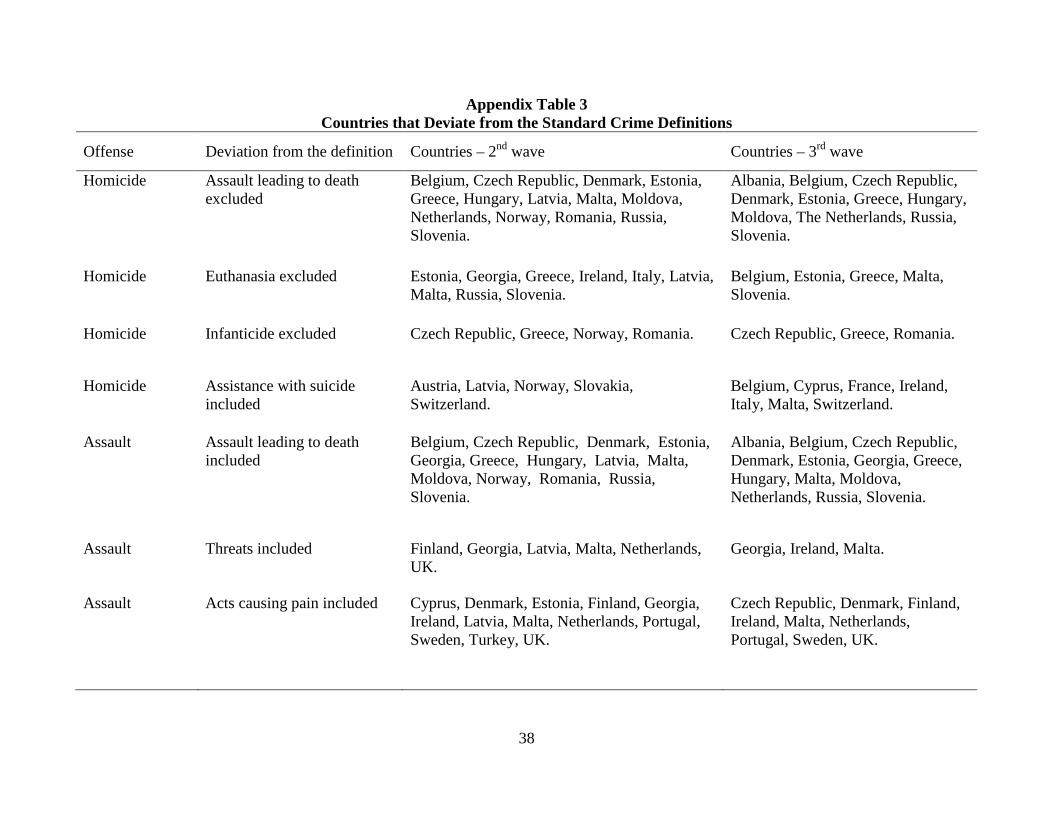
For all crimes included in the European Sourcebook, a standard definition is used and the

statistics follow this standard definition where possible. These definitions are provided in

Appendix Table 2. If a country’s crime statistics deviate from the standard definition, the

European Sourcebook provides information about what aspect of the standard definition is not

met. For example, the standard definition of homicide is “intentionally killing of a person.”

8 In most of the European countries the police and public prosecutors use discretion to decide whether to prosecute or not. For example, the criminal can get away with a warning for small scale thefts or burglaries. Most importantly, the crime definitions used by the judicial system and the police are not identical. Although offence definitions adopted by the various police systems present uniformity among countries, rules for recording punishments can vary substantially. 9 Source: World Bank, World Development Indicators. 10 For example, the United Nations Surveys of Crime Trends and Operations of Criminal Justice Systems provide data reported by law enforcement agencies in each country. The crime statistics in the U.N. dataset are not standard across countries, unlike the European Sourcebook data.

10

According to this definition, euthanasia should be included as homicide, since euthanasia

involves intentionally killing of a person in order to relieve pain and suffering. However,

euthanasia is not considered a homicide by some countries and it is impossible for these

countries to provide homicide data that include euthanasia cases. The European Sourcebook lists

the countries that follow the standard definition and also those that do not follow. The countries

that deviate from the standard crime definitions and the way they deviate from the standard

definitions are listed in Appendix Table 3. In the empirical analysis, any non-conformity to

definitions is controlled for by a set of dummy variables.11

The source of labor market variables, GDP per capita and urban population is the World

Development Indicators.12 The ratio of young population to the old population is the ratio of

population aged 15-39 to the population aged 40 or more. It is constructed using the data from

the U.S. Census Bureau's International database.13 Alcohol consumption per capita variable is

obtained from the World Health Organization’s Global Alcohol Database.14 Drug crime rate and

the police rate are crimes related to drugs and police officers per 100,000 individuals,

respectively. They are obtained from the European Sourcebook. Table 1 presents the definitions

and the descriptive statistics of all the variables as well as their sources.

Among the instrumental variables, exchange rate is obtained from the Penn World Tables

version 6.3. Exchange rate is measured as the amount of domestic currency that one US dollar 11 Specifically, I include indicator variables that take the value of one if the crime statistics for a country and year deviates from the standard definition in the way mentioned in the Appendix Table 3. For example, the standard definition of homicide imposes that euthanasia should be considered a homicide. However, homicide statistics of Estonia, Georgia, Greece, Ireland, Italy, Latvia, Malta, Russia, Slovenia in the second wave of the European Sourcebook (1995-1999) and those of Belgium, Estonia, Greece, Malta, and Slovenia in the third wave of the European Sourcebook (2000-2003) excludes euthanasia. Consequently, in the murder regressions I include an indicator variable that takes the value of one for these countries and years. Such a variable captures the differences between and within the countries in murder statistics due to exclusion of euthanasia. Similar indicator variables are included in the relevant regressions for each of the deviation from the standard definition reported by the European Sourcebook. The deviations are reported in the Appendix Table 3. 12 http://data.worldbank.org/indicator 13 http://www.census.gov/ipc/www/idb/ 14 http://www.who.int/globalatlas/default.asp

11

can buy. Share of manufacturing sector’s value added in GDP is obtained from World

Development Indicators. Finally, the data on industrial accidents and earthquakes are obtained

from EM-DAT data base (the international disaster data base).15 More details about the

instruments are provided in the Instrumental Variables section below.

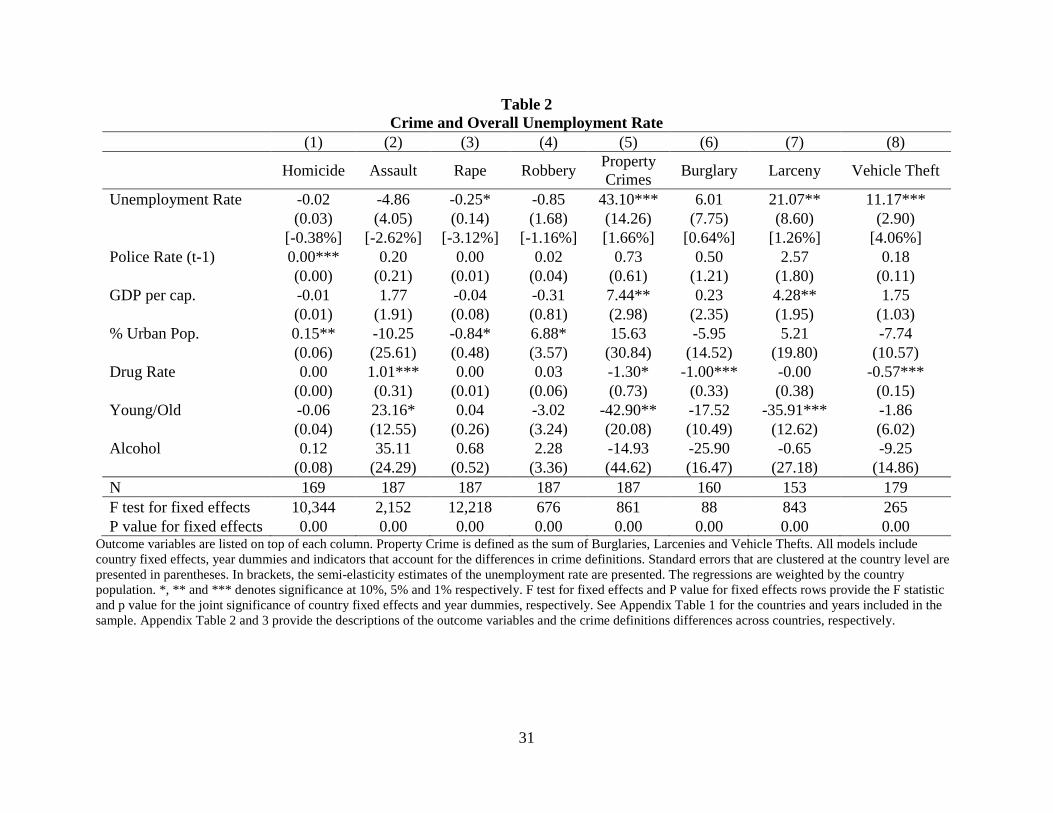
OLS Results

Overall Unemployment Rate

Figure 1 provides a visual presentation of the influence of the unemployment rate on

crime. In Figure 1, a measure of property crime rate and the unemployment rate for the set of the

countries with non-missing data are depicted. Property crime rate is chosen as it includes all

burglaries, larcenies and motor vehicle thefts together. The graphs of individual crime types are

similar to that of property crimes. The solid line represents the variation in the property crime

rate that is unexplained by the control variables. Specifically, the measure of the property crime

rate depicted in Figure 1 is obtained by calculating the residuals from the regression of property

crime rate on control variables used in the empirical analysis.16 The dashed line is the

unemployment rate.

Among the graphs of the 16 countries presented in Figure 1, most graphs show that the

unemployment rate and the property crime rate have very similar trends. Graphs of seven

countries (UK, Switzerland, Sweden, Poland, Italy, Hungary and Finland) display an obvious

positive partial correlation between the unemployment rate and the property crime rate for the

15 http://www.emdat.be/ 16 The control variables are Lagged Police Rate, GDP per capita, % Urban Population, Drug Rate, Young per Old population and Alcohol consumption per capita as well as country fixed effects, year dummies and indicators that account for the differences in crime definitions.

12

whole sample period.17 Another 6 graphs (Slovenia, Portugal, Ireland, Denmark, Czech Republic

and Croatia) reveal positive partial correlation for some years in the sample.

To quantify the relationship between unemployment and crime observed in Figure 1, I

regress the crime rates on the unemployment rate and the control variables using OLS. The

crimes considered are homicide, assault, rape, robbery, total property crimes, burglary, larceny

and motor vehicle theft.18 The variable of interest in this section is the unemployment rate.

Control variables include lagged police rate, GDP per capita, % urban population, drug rate,

young per old population and alcohol consumption per capita. The regressions also control for

country fixed effects and year dummies as well as indicators that account for the differences in

crime definitions. Standard errors that are clustered at the country level are reported in

parentheses. Regressions are weighted by the country population.19 The results are provided in

Table 2.

Being unemployed can induce motivation to earn income illegally, but it does not

necessarily increase violent behavior. The estimates in Table 2 support this hypothesis. The sign

of the unemployment rate’s coefficients are positive for all crimes that involve pecuniary

benefits except robbery. Further, this influence is statistically significant for total property

crimes, larcenies and motor vehicle thefts. A one percentage point increase in the unemployment

rate is associated with 2%, 1% and 4% increase in total property crimes, larcenies and motor

vehicle thefts, respectively.20 These results are consistent with previous studies that employ US

data, such as Lin (2008), Gould, Weinberg and Mustard (2002) and Levitt (2004). The

17 In this study UK refers to England and Wales. 18 The definitions of these variables are presented in Appendix Table 2. 19 The weights are the average country population in the sample period. 20 Similar elasticities are estimated when natural log of the crimes are used instead of the level of the crime. When standard errors are corrected for first-order serial correlation, the coefficients of the unemployment rate in total property crime, larceny and motor vehicle theft regressions are significant at conventional levels and the estimated elasticities are similar to those reported in Table 2.

13

unemployment rate is not significantly associated violent crimes. The negative sign of the

unemployment rate in violent crime regressions is not uncommon in the literature. For example,

OLS estimates in Lin (2008) show the same exact pattern.

GDP per capita is positively associated with property crimes but not with violent crimes.

This may be because GDP per capita is a proxy for the benefits associated with crimes. The

greater is the average income in a country, the greater returns to committing property crimes are

on average. Along the similar lines, the coefficient of Young per Old for crimes that involve

monetary benefits is negative. This variable may be indicative of wealth in a country. Generally

wealth is accumulated over the life cycle and the elderly have more valuable assets compared to

the young. If in a country there are more young individuals for each elderly individual, then there

is less to steal.21

The coefficient of Drug Crime Rate is consistently positive for violent crimes and

negative for property crimes.22 This pattern may arise because drug crimes can be substitutes for

property crimes, but complements for violent crimes. Individuals who choose to work in illegal

sector allocate their time between several illegal income-generating activities. The criminals

whose net returns to drug crimes are greater than net returns to property crimes are less likely to

commit larceny, burglary or motor vehicle theft. They rather earn income through drugs.

A similar pattern is observed for the coefficient of the Alcohol consumption. Alcohol

consumption per capita is correlated positively with violent crimes and negatively with property

crimes. A possible explanation of this pattern involves the impact of alcohol on individual

behavior. First, excessive alcohol consumption is associated with more aggressive and violent

21 On the other hand, it is well-known that the young are more likely to commit crimes compared to the old. In fact, this is reflected in the positive coefficient of Young per Old in the Assault regression. The greater the ratio of young individuals to old individuals is, the greater the number of assaults which has no monetary rewards to the offender. 22 The Drug Crime Rate is not only a proxy for the prevalence of drug use and possession, but also a measure of the extent of illegal income-generating activities related to drugs.

14

behavior (Markowitz 2005). Secondly, individuals who consume large amounts of alcohol may

suffer from judgment impairment and diminished physical performance. These and other

mechanisms that relate alcohol consumption and criminal activity are discussed in Carpenter and

Dobkin (2010). The side effects of alcohol consumption are reflected in the estimated

coefficients of alcohol. Potential criminals under the influence of alcohol are less likely to

effectively carry out activities related to property crimes. In fact, several property crimes require

some skills such as opening a locked door (in case of a burglary) or starting a car without keys

(in case of motor vehicle theft).

Although most of variables’ coefficients exhibit the expected signs, police rate and

urbanization rate do not. Nevertheless, those variables are not the variables of interest. Notice

that these control variables are included in the regressions to isolate the influence of the

unemployment rate on crime through mechanisms other than legal labor market opportunities.

The reason for the unexpected coefficient signs may be due to imprecise estimation as these

control variables may be a noisy measure. Therefore, I do not put much stake on these

coefficients.23

The sample I employ contains countries with both stable and unstable democracies.

Using a country-level data set, Lin (2007) shows the level of democracy in a country is a

significant determinant of crime. If the regime type in a country also influences the

unemployment rate, then my estimation will be biased. Further, the influence of unemployment

rate on crime may be different in democratic versus less democratic countries.24 To investigate

these possibilities, I obtained the Democracy index of the countries in my sample from Polity

23 Similarly, some previous studies had positive coefficients for police in crime regressions. Examples include Cornwell and Trumbull (1994). 24 I thank an anonymous referee for pointing this out.

15

IV.25 The Democracy index ranges between -10 (strongly autocratic) and 10 (strongly

democratic). European countries in my sample were mostly strongly democratic countries with

median Democracy level of 10. I construct an indicator variable that takes the value of one if a

country’s average democracy level during the years covered is equal to 10. 18 countries’ average

democracy levels are 10 the sample.26 In addition to all of the control variables mentioned above,

I included the democratic country indicator and its interaction with the unemployment rate in the

regressions. The coefficients of the unemployment rate variable remain unaffected, while the

interaction term is insignificant. The sum of the interaction term and the unemployment rate is

also positive and significant at conventional levels. These results indicate that there is no

systematic difference between the strongly democratic and less democratic countries in terms of

the influence of the unemployment rate on crime. In other words, findings reported in this

section are not driven by the countries with stable democracies.

Many mechanisms can motivate a positive influence of migration on crime. For example,

migrants are more likely to be poorly-educated and to be discriminated against. Customers may

reveal distaste against migrants. Alternatively, migrants may be less productive in some

industries. All of these mechanisms may cause migrants to have less lucrative labor market

opportunities and consequently lead them to involve in criminal activity. As a result, exclusion of

a measure of migration may result in biased estimates if migration influences both

unemployment and crime.27 To prevent against this possibility, I include the share of migrants in

country population in the regressions. The results are virtually unchanged. Despite a slight

decrease, the magnitude and significance of the unemployment rate remain almost identical to

25 http://www.systemicpeace.org/polity/polity4.htm 26 These countries are Austria, Belgium, Cyprus, Czech Republic, Denmark, Finland, Greece, Hungary, Ireland, Italy, Lithuania, Netherlands, Norway, Portugal, Slovenia, Sweden, Switzerland and UK. 27 I thank another anonymous referee for pointing this out.

16

Table 2 for property crimes. The share of migrants does not significantly influence any crime

except motor vehicle theft. The coefficient of the share of migrants is negative and significant for

motor vehicle thefts.28

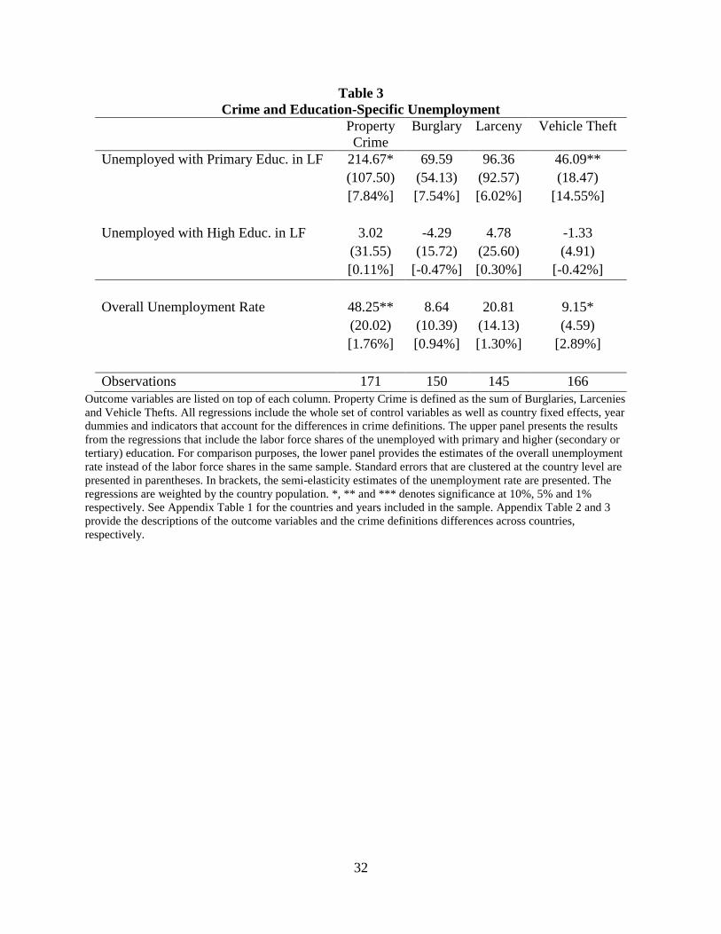
Education-Specific Unemployment

As discussed by Raphael and Winter-Ebmer (2001) and Lin (2008), the overall

unemployment rate may not be able to identify the marginal criminal. Individuals who belong to

two different population sub-groups (such as the highly-educated versus poorly-educated) and

who are financially at the margin of committing a crime may respond differently when they

become unemployed. For example, Becker and Mulligan (1997), Lochner (2004), and Lochner

and Moretti (2004) have suggested that greater schooling decreases criminal activity.

Furthermore, Grogger (1998) and Gould, Weinberg and Mustard (2002) report that unskilled and

uneducated males respond to changes in their employment statuses most significantly by

committing crimes.

In this section, the overall unemployment rate is decomposed into education-specific

unemployment measures. This allows me to gauge the differential impacts on crime of the

unemployment of individuals with higher and lower levels of education. Specifically, instead of

the overall unemployment rate, the shares of the unemployed people with primary education and

high education in the labor force are included in regressions.29 Since individuals with primary

education have worse labor market prospects than high educated individuals, the relationship

28 The coefficient of migrants share is negative but insignificant for other property crimes. This result may be due to migrants’ poverty. Migrants are associated with low levels of income and wealth. After all, poverty may be one reason why they migrate to another country. Therefore, an increase in the share of migrants in a country implies fewer pecuniary benefits of committing a crime on average. 29 Labor force share of the unemployed with primary education (high education) is the ratio of the unemployed individuals who has completed primary education (who has completed secondary or tertiary education) to the total labor force.

17

between crime and the unemployment of individuals with primary education is expected to be

stronger.

Table 3 displays the results. In the upper panel, results for total property crimes, burglary,

larceny and motor vehicle theft are summarized. For comparison purposes, the lower panel

presents the estimates from the specification where the overall unemployment rate is included

instead of the labor force share variables. The sample sizes in these regressions are smaller due

to missing education-specific unemployment data. Consequently, in Table 3, the coefficients

estimates of the overall unemployment rate are different from those reported in Tables 2.

Results presented in Table 3 provide evidence that unemployed individuals with primary

education are more influential in the effect of unemployment on crime. A one percentage point

increase in the labor force share of the unemployed with low education leads to about 7% and

16% increase in total property crimes and motor vehicle thefts, conditional on the unemployment

of the high educated individuals.30 The influence of the labor force share of the unemployed with

low education is greater than that of the unemployed with high education in magnitude for all

property crimes. The difference is statistically significant for total property crimes and motor

vehicle thefts.31

30 These elasticity estimates are consistent with the estimates of the overall unemployment rate. For example, a one percentage point increase in the overall unemployment rate is associated with two percent increase in the total property crime rate. In this sample, on average, one third of the all unemployed individuals have at most primary education. If individuals with low education and high education are equally likely to be laid off for example due to a recession, a one percentage point increase in the unemployment rate leads to a one third percentage point increase in the unemployment of individuals with primary education. According to the estimates in Table 3, such a change will lead to a two percent increase in the total property crime rate (six percent multiplied by one third). 31 However, the impact of education specific unemployment on violent crimes is statistically not different than zero with very high p-values. The results are not presented.

18

5. Instrumental Variables

As discussed in the Empirical Framework section, unemployment can be endogenous in a

crime regression. Although using a country-level panel data set minimizes this concern, there may be

other reasons that motivate IV estimation such as measurement errors and unobserved confounding

factors. Therefore, I estimate IV models where the unemployment rate is instrumented by several

instrumental variables.

First instrument is the exchange rate weighted by the manufacturing sector’s value added

to the country’s GDP in previous year. This instrument is similar to the one used by Lin (2008)

for his analysis of crime and unemployment in US, and by Oster and Agell (2007) for their

analyses of crime and unemployment in Sweden. The impact of the exchange rate on the

unemployment rate is theoretically well-founded.32 When the exchange rate appreciates, goods

and services in the country become more expensive compared to the rest of the world. This leads

to a decrease in foreign demand for domestic goods and an increase in domestic demand for

foreign goods. As a result, exports and eventually production in the domestic country declines

which increases the unemployment rate. That is, if the exchange is calculated as the amount of

domestic currency per U.S. dollar, then theoretically there should be an inverse relationship

between the exchange rate and the unemployment rate. Following the previous literature, I

weighted the exchange rate movements with the manufacturing sector’s value added in previous

year.

The second and third instruments are constructed based on disasters experienced by

countries. Data on occurrence of such disasters are obtained from EM-DAT (the international

disaster data base).33 For an event to be included in the EM-DAT database as a disaster, it has to

32 See the studies cited by Lin (2008) for a review. 33 http://www.emdat.be/

19

satisfy certain criteria. First, the event must be unforeseen and sudden. Because of this criterion,

the events included in the EM-DAT database are unquestionably random. Secondly, the event

must fit at least one of the following categories: A) 10 or more people got killed; B) 100 or more

people got affected34; C) the affected country declared a state of emergency; D) the affected

country called for international assistance. Consequently, the events listed in the EM-DAT

database can be considered to have caused great damage, destruction and human suffering.

One of the instruments that are created based on disasters is the occurrence of industrial

accidents in a country. EM-DAT defines an industrial accident as a technological accident of an

industrial nature or involving industrial buildings such as factories. Examples of industrial

accidents include collapse or explosion of mines, destruction of industrial buildings or

infrastructure and spill of hazardous/chemical materials. The list of industrial accidents in the

sample used is presented in Appendix Table 4.

Industrial accidents can be related to employment through two mechanisms. First,

industrial accidents lead to shut-down of a plant/factory and therefore cause termination of

employment of the workers. Secondly, because of the spill-over effects, employment in other

plants/factories may be affected as well. Specifically, the production of the businesses that use

the output of the closed plant/factory as an input in their production is expected to reduce.

Similarly, the production of the businesses that supply inputs to the closed factory/plant is

expected to decrease. Consequently, the employment in such businesses is likely to decrease as

well as the employment in the firm affected by the accident.

34 According to the EM-DAT, a person is considered affected if he/she has required immediate assistance during a period of emergency, i.e. requirement of basic survival needs such as food, water, shelter, sanitation and immediate medical assistance.

20

The mechanism can be explained better using an example of, say, a coal mine and a

transportation company that delivers the coal from the mine to other locations. When the coal

mine collapses, the production of the coal mine stops or gets reduced. This reduces the

employment in the coal mine. Further, the services of the transportation company will not be

needed which may lead to a reduction of employment in the transportation company. The

collapse of the coal mine will also reduce the employment in other businesses which use coal as

an intermediate good.

As a result, an increase in the unemployment rate is expected due to the industrial

accidents. The influence of industrial accidents on unemployment must be greater for the

countries with greater employment in manufacturing sector. Other things equal, manufacturing

employment is greater in the countries whose contribution of the manufacturing sector to the

GDP. As a result, I use the interaction of the indicator variable for the occurrence of industrial

accidents in a country with the share of manufacturing sector’s value-added to GDP in previous

year as an instrument.

The third instrument is the occurrence of earthquakes. An earthquake is defined as the

shaking and displacement of ground due to seismic waves by EM-DAT. As mentioned above,

these earthquakes were large enough to influence the lives of many individuals. The list of

earthquakes (observed by EM-DAT) used in the analysis is provided in Appendix Table 5.

Generally speaking, in the area where an earthquake is observed, buildings and the

infrastructure are destroyed or damaged and people are killed or injured and so on. Therefore,

the initial influence of an earthquake in the local area where it is observed is a reduction in

employment. There are multiple studies which show that the area struck by an earthquake suffers

extensive economic losses. For example, Cavallo, Powell and Becerra (2010) show that the Haiti

21

earthquake of 2010 has cost at least eight billion dollars to Haitians. Holden, Bahls, and Real

(2007) forecast that an earthquake with a magnitude of 6.9 in the Bay Area in Northern

California could result in a loss of employment in the Bay area by about 420,000.

Although the initial effect of disasters such as earthquakes can be devastating in the local

area affected, in the longer run both the local and the aggregate labor market improve. That is,

despite its initial damage on the local areas, an earthquake can improve the economic conditions

in the country as a whole in the longer run. The mechanism involves the reconstruction efforts in

the shaken locality. Specifically, in the local area hit by an earthquake, the demand for goods and

services such as demand for health care and especially construction services go up. In such a

case, employment opportunities for those individuals who are not affected by the earthquake can

get improved. This is demonstrated by Pereira (2009) who studies the economic impact of 1755

Lisbon Earthquake which is the largest natural catastrophe ever recorded in Europe. Pereira

(2009) argues that the earthquake lead to a rise in the wage premium of construction workers due

to the reconstruction efforts. Using evidence from hurricanes (which can have similar effects as

earthquakes), Ewing and Kruse (2005) suggest that “hurricanes may have a short run adverse

impact on a community; however, these storms may also be associated with a long run positive

impact on economic activity.” Similarly, Ewing, Kruse and Thompson (2009) argue that 1999

Oklahoma City tornado led to improvements in the labor market at the aggregate level. In the

light of the evidence provided above, an earthquake is expected to reduce the annual

unemployment rate in a country.35

35 Using earthquakes as an instrument, I assume that earthquakes do not directly influence crime, but only through the changes through the unemployment rate. This is indeed in line with the previous research. For example, using the Hurricane Katrina which was very destructive for New Orleans, Varano et.al. (2010) argue that there were not significantly large increases in the crime rates of Houston, San Antonio, and Phoenix which received largest numbers of displaced New Orleans residents due to Hurricane Katrina. Moreover, since the number of instruments is greater than the number of endogenous variables, I conduct test for over-identifying restrictions. In this test, the null

22

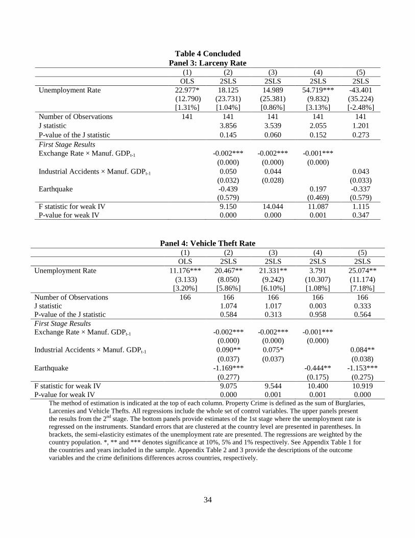
The 2SLS estimates of the impact of the unemployment rate on total property crimes,

burglaries, larcenies and motor vehicle thefts are presented in Panels 1 to 4 of Table 4. Panels for

each crime also provide the first stage results and test statistics pertaining to validity and strength

of the instruments (F statistic for the strength and J statistic for the validity). Notice that there are

differences between the samples used in each panel. Due to the unavailability of the outcome

variable, the sample sizes of burglary and larceny rate are much smaller than sample sizes of the

total property crime and motor vehicle theft rates. 36 In the first column of each panel, the OLS

estimate of the unemployment rate is given for comparison purposes. In each panel, columns 2 to

5 provide the 2SLS estimates where a different combination of the instruments is used in the first

stage. Specifically, second columns present the estimates of 2SLS model where exchange rate,

industrial accidents and earthquakes are included as instruments jointly. In columns 3, 4 and 5,

exchange rate and industrial accidents; exchange rate and earthquakes; and industrial accidents

and earthquakes are used as instruments, respectively.

For all samples the interaction of the exchange rate with the lagged manufacturing share

of GDP is a strong instrument. The other instruments, industrial accidents and earthquakes are

not always strong. Especially for the Burglary rate (Panel 2) and Larceny rate (Panel 3) samples,

earthquakes and industrial accidents are not significant determinants of the unemployment rate.

This is due to the reduced variation in industrial accidents and earthquakes in burglary rate and

larceny rate samples.37 Nonetheless, the F-statistic for the instruments in the first stage is around

hypothesis is that the instruments are valid instruments, and that the excluded instruments are correctly excluded from the estimated equation. The instruments used in the paper pass this test. 36 Depending on the availability of the outcome variable, the sample sizes differ for each panel. Also sample size in Table 4 is smaller than the size of the sample used in Table 2 (OLS results). This is due to the missing data on instruments for some years and countries. 37 For example, the sign of the industrial accident in the first stage is always positive in all samples but insignificant in burglary and larceny samples. This is just due to the smaller sample size. Table 4 presents change of sign for earthquake. This is due to fact that Greece and Italy are not in the burglary and larceny samples. Greece and Italy account for about half of the earthquakes in the estimation sample. See Appendix Table 5 for details.

23

10 which is the rule of thumb threshold for a weak instrument suggested by Stock and Watson

(2003).38 Admittedly, in some cases, the instruments barely pass this threshold. However, the

lowest F-statistic is about 9 (excluding the specification in the 5th columns of Panels 2 and 3 with

smaller samples and weaker instruments of industrial accidents and earthquakes). In addition,

Table 4 presents the J-statistic. This is a test of over-identifying restrictions.39 With the exception

of the larceny rate in Panel 3, all of the crime categories pass the over-identification test.

Moreover, most of the J-statistics are smaller than two. This indicates that the 2SLS method is

insensitive to the choice of instrumental variables.

According to the OLS estimates in columns 1 of each panel, a one percentage point

increase in the unemployment rate is associated with 1.7%, 0.8%, 1.3%, 3% increase in total

property crimes, burglaries, larcenies and motor vehicle thefts. 2SLS estimation (columns 2-5)

produces larger point estimates. For example, the 2SLS estimations of unemployment elasticity

for the property crime rate using different sets of instrumental variables range from 2.4 to 3.8

percent. These estimates are larger than the OLS estimates. Similar results are obtained for other

crime categories as well. For example, the 2SLS estimates of unemployment elasticity of

burglary rate range between 2.8 and 4.2 percent and of motor vehicle theft rate between 5.7 and 7

percent.

6. Economic Impact of Crime Due to Recessions

In this section, I simulate the economic impact of the increase in crime due to a one

percentage point increase in the unemployment rate. The back-of-the-envelope calculations rely

38 The null hypothesis is that all coefficient estimates of the instrumental variables in the first-stage regression are not jointly different from zero. 39 The null hypothesis is that the instruments are valid instruments, and that the excluded instruments are correctly excluded from the estimated equation.

24

on the cost of crime estimates of Anderson (1999) who decomposes the aggregate burden of

crime into several components.

Based on Anderson (1999)’s estimates, I calculate each property crime costs about

$46,000 in US in 1999 dollars. The calculations are summarized in Appendix Table 6. The OLS

estimates in this paper (similar to those in previous studies) suggest that a one percentage point

increase in the unemployment rate is associated with about one to two percent increase in

property crimes. Consequently, a one percentage point rise in the overall unemployment rate

translates into about 25,000-30,000 extra property crimes for a country with population similar to

France, Italy or UK (50-60 million). Therefore, for each percentage point increase in the

unemployment rate, the French, Italians and Britons incur about $1.2 – $1.4 billion additional

cost due to crime.

The 2SLS estimates in this paper draw a more pessimistic picture. According to the 2SLS

estimates, a one percentage point increase in the unemployment rate increases property crime

rate by about 2.4 – 3.8%. These elasticities translate into about $1.6 – $2.5 billion additional cost

of crime for Italy, France or UK due to the increase in the unemployment rate by one percentage

point.

7. Summary and Conclusion

This paper investigates the impact of unemployment on crime using a panel data set of 33

European countries, and it is one of the few papers which studies crime in an international

context. The primary advantage of the data set is that it contains consistently measured crime

variables across countries and over time.

25

The findings presented in this paper are consistent with the previous literature. I find that

a one percentage point increase in the unemployment rate increases property crimes by about 2

percent using OLS. Instrumenting the unemployment rate using the exchange rate, industrial

accidents and earthquakes produces larger point estimates. This finding is similar to that of the

previous research (Lin 2008 and Raphael Winter-Ebmer 2001).

Because the overall unemployment rate may not be able to identify people on the margin

of committing a crime (Lin 2008 and Raphael Winter-Ebmer 2001), the influence of education-

specific unemployment on crime is investigated. The overall unemployment rate is decomposed

into labor force shares of the unemployed with primary education and high education. The

results show that the unemployment of individuals with low education is a significant

determinant of the impact of the unemployment rate on crime.

The magnitude of the unemployment’s impact on crime is economically significant. For

example, France, Italy or UK suffer about 25,000-30,000 additional larcenies, burglaries and

motor vehicle thefts per year for one percentage point increase in the unemployment. Roughly,

cost of each property crime is $46,000. Due to one percentage point increase in the

unemployment rate, the French, Italian and British incur an extra crime cost of about $1.2-$1.4

billion according to the OLS estimates or $1.6 – $2.5 billion according to the 2SLS estimates.40

40 See Appendix Table 6 and section 6 for the details of this calculation.

26

References

Anderson, D., 1999. The aggregate burden of crime. Journal of Law and Economics 42 (2), 611-42.

Becker, G. S., 1968. Crime and punishment: an economic approach. The Journal of Political Economy 76 (2), 169-217.

Becker, G. S., Mulligan, C. B., 1997. The endogenous determination of time preference. Quarterly Journal of Economics 112 (3), 729-58.

Block, M., Heineke, M., 1975. A labor theoretic analysis of the criminal choice. American Economic Review 65 (3), 31425.

Bianchi, M., P. Buonanno, and P. Pinotti. 2011. Do immigrants cause crime?. Journal of the European Economic Association. Forthcoming.

Buonanno, P. 2006, Crime and labor market opportunities in Italy (1993-2002), Labour 20(4):601-24.

Cavallo, Eduardo; Powell, Andrew; Becerra, Oscar. 2010. “Estimating the Direct Economic Damages of the Earthquake in Haiti.” Economic Journal 120(546), pp. F298-312.

Carpenter, C. and Dobkin, C. 2010. Alcohol regulation and crime. NBER Working Paper Series No. 15828.

Corman, H., Mocan, H. N., 2000. A time-series analysis of crime, deterrence, and drug abuse in New York City. The American Economic Review 90 (3), 584-604.

Corman, H. and Mocan N. 2005. Carrots, sticks and broken windows. Journal of Law and Economics 48(1), pp.235-66.

Cornwell, C. and Trumbull W. 1994. Estimating the economic model of crime with panel data. The Review of Economics and Statistics 76(2), pp. 360-366.

Cullen, J. B., Levitt, S. D., 1999. Crime, urban flight, and the consequences for cities” The Review of Economics and Statistics 81 (2),159-69.

Edmark, K. 2005, Unemployment and crime: is there a connection? Scandinavian Journal of Economics 107(2):353-73.

Ehrlich, I. 1973. Participation in illegitimate activities: a theoretical and empirical investigation. Journal of Political Economy 81 (3), 52165.

Engelhardt, E. 2010. The effect of employment frictions on crime. Journal of Labor Economics 28(3), pp. 677-718.

EU ICS, The burden of crime in the EU, a comparative analysis of the European survey of crime and safety 2005”.

27

Ewing, Bradley T. and Jamie B. Kruse. 2005. “Hurricanes and unemployment.” East Carolina University Center for Natural Hazards Research Working Paper 0105-002.

Ewing, Bradley T., Jamie B. Kruse and Mark A. Thompson. 2009. “Twister! Employment responses to the 3 May 1999 Oklahoma City tornado.” Applied Economics 41, pp.691-702.

Fajnzylber, P., Lederman, D., Loayza, N., 2000. What causes violent crime? European Economic Review 46 (7), 1323-1357.

Fajnzylber, P., Lederman, D., Loayza, N., 2002. Inequality and violent crime. Journal of Law and Economics 45 (1), 1-40.

Freeman, R. B.. 1995. Why do so many young American men commit crimes and what might we do about it? The Journal of Economic Perspectives 10, 25-42.

Gould, E. D., Weinberg, B. A., Mustard, D. B., 2002. Crime rates and local labor market opportunities in the United States: 1979-1997. The Review of Economics and Statistics 84 (1), 45-61.

Grogger, J., 1998. Market wages and youth crime. Journal of Labor Economics 16 (4), 756-91.

Holden, Richard J., Bahls, Donna and Real, Charles. 2007. “Estimating Economic Losses in the Bay Area from a Magnitude-6.9 Earthquake.” Monthly Labor Review 130(12), pp.16-22.

Kelly, M., 2000, Inequality and Crime, The Review of Economics and Statistics 82 (4), 530–539.

LaGrange, T. C., and Silverman, R. A., 1999. Low self-control and opportunity: testing the general theory of crime as an explanation for gender differences in delinquency.” Criminology 37 (1), 41-72.

Levitt, S. 1997. Using electoral cycles in police hiring to estimate the effect of police on crime. The American Economic Review 87(3), pp.270-290.

Levitt , S. 2004. Understanding why crime fell in the 1990s: Four factors that explain the decline and six that do not. Journal of Economic Perspectives 18(1), pp. 163-190.

Lin, Ming-Jen. 2007. Does democracy increase crime? The evidence from international data. Journal of Comparative Economics 35, 467-483.

Lin, Ming-Jen. 2008. Does unemployment increase crime? Evidence from U.S. data 1974–2000. Journal of Human Resources 43 (2),413–436.

Lin, Ming-Jen. 2009. “More Police, Less Crime: Evidence from US State Data", International Review of Law and Economics 29(2), pp. 73-80

Lochner, L., 2004. Education, work, and crime: a human capital approach. International Economic Review 45 (3), 811-843.

Lochner, L., Moretti, E., 2004. The effect of education on crime: evidence from prison inmates, arrests, and self-reports. The American Economic Review 94 (1), 155-89.

28

Machin, S., Meghir, C., 2004. Crime and economic incentives. The Journal of Human Resources 39 (4), 958-79.

Markowitz, S. 2005. Alcohol, drugs and violent crime. International Review of Law and Economics 25(1), pp. 20-44.

Miron, Jeffrey. 2001. Violence, guns, and drugs: a cross-country analysis. Journal of Law and Economics 44(S02), pp.615-33.

Mocan, Naci. 1999. Structural unemployment, cyclical unemployment and income inequality. The Review of Economics and Statistics 81(1), pp.122-34.

Mocan, N., Billups, S., Overland, J., 2005. A dynamic model of differential human capital and criminal activity. Economica 72, pp. 655-81.

Oster, A. and J. Agell, 2007. Crime and unemployment in turbulent times, Journal of the European Economic Association 5(4):752-75.

Pereira, Alvaro S. 2009. “The opportunity of a disaster: the economic impact of the 1755 Lisbon Earthquake.” Journal of Economic History 69(2), pp. 466-99.

Raphael, S., Winter-Ebmer, R., 2001. Identifying the effect of unemployment on crime. Journal of Law and Economics 44 (1), 259-83.

Ruhm, Christopher J. (1995), economic conditions and alcohol problems. Journal of Health Economics 14, 583-603.

Soares, R. R., 2004. Development, crime and punishment: accounting for the international differences in crime rates. Journal of Development Economics 73 (1), 155-184.

Varano, Sean, Joseph Schafer, Jeffrey Cancino, Scott Decker, and Jack Greene. 2010. A tale of three cities: Crime and displacement after Hurricane Katrina. Journal of Criminal Justice 38, pp.42-50.

Witte, Ann D. 1980. Estimating the Economic Model of Crime with Individual Data. Quarterly Journal of Economics 94, pp. 57-84

Wolpin, K. I., 1980. A time series-cross section analysis of international variation in crime and punishment” The Review of Economics and Statistics 62 (3), 417-23.

29

Table 1 Summary Statistics and Descriptions

Variable Definition Source N Mean Std. Dev. Homicide Rate* Homicides per 100,000 individuals. A 169 5.28 3.94

Assault Rate* Assaults per 100,000 individuals. A 187 185.83 239.54 Rape Rate* Rapes per 100,000 individuals. A 187 8.01 6.41

Robbery Rate* Robberies per 100,000 individuals. A 187 73.74 67.75 Property Crime Rate* Sum of larcenies, burglaries and vehicle thefts per 100,000

individuals. A 187 2618.52 1991.86

Burglary Rate* Burglaries per 100,000 individuals. A 160 938.69 681.00 Larceny Rate Difference between the Property Crime Rate and the sum

of Burglary Rate and Motor Vehicle Theft Rate. A 153 1668.26 1339.17

Motor Vehicle Theft* Thefts of motor vehicles per 100,000 individuals. A 179 275.10 238.89 Unemployment Rate Ratio of unemployed population to labor force times 100. B 187 8.52 4.25

Share of the Poorly-Educated and Unemployed in Labor Force

Ratio of unemployed population with at most primary schooling to total labor force times 100.

B 172 2.67 1.58

Share of the Well-Educated and Unemployed in Labor Force

Ratio of unemployed population with more than primary schooling to total labor force times 100.

B 171 5.71 3.67

Lagged Police Rate Total number of police officers per 100,000 people A 187 349.21 168.69

GDP per capita Real GDP per capita in 2000 dollars. Scaled by 0.01. B 187 207.47 105.81 % Urban Population Ratio of the population living in urban areas to the total

population times 100. B 187 67.25 12.81

Drug Rate Crimes related to drugs per 100,000 individuals. A 187 145.55 180.67 Alcohol Alcohol consumption per capita per annum, in liters. C 187 9.69 3.09

30

Table 1 Continued Variable Definition Source N Mean Std. Dev. Young/Old Ratio of population aged 15-39 to the population aged

more than 40 times 100. D 187 83.09 9.80

Exchange Rate × Manuf. GDPt-1 Exchange rate weighted with the share of manufacturing sector’s value added to GDP

F, B 175 372.83 1155.74

Industrial Accidents × Manuf. GDPt-1

Dummy for industrial accidents weighted with the share of manufacturing sector’s value added to GDP

E,B 175 1.60 5.65

Earthquake Dummy for earthquakes E 187 0.09 0.29

* See Appendix Table 1 for the standard definitions and the Appendix Table 2 for the deviations of the countries from the standard definition A – European Sourcebook of Crime and Criminal Justice, B – World Development Indicators, C – World Health Organization, Global Alcohol Database,

D – U.S. Census Bureau, International Database, E – EM-DAT, the international disaster data base.

31

Table 2 Crime and Overall Unemployment Rate

(1) (2) (3) (4) (5) (6) (7) (8)

Homicide Assault Rape Robbery Property Crimes Burglary Larceny Vehicle Theft

Unemployment Rate -0.02 -4.86 -0.25* -0.85 43.10*** 6.01 21.07** 11.17***

(0.03) (4.05) (0.14) (1.68) (14.26) (7.75) (8.60) (2.90)

[-0.38%] [-2.62%] [-3.12%] [-1.16%] [1.66%] [0.64%] [1.26%] [4.06%] Police Rate (t-1) 0.00*** 0.20 0.00 0.02 0.73 0.50 2.57 0.18

(0.00) (0.21) (0.01) (0.04) (0.61) (1.21) (1.80) (0.11)

GDP per cap. -0.01 1.77 -0.04 -0.31 7.44** 0.23 4.28** 1.75

(0.01) (1.91) (0.08) (0.81) (2.98) (2.35) (1.95) (1.03)

% Urban Pop. 0.15** -10.25 -0.84* 6.88* 15.63 -5.95 5.21 -7.74

(0.06) (25.61) (0.48) (3.57) (30.84) (14.52) (19.80) (10.57)

Drug Rate 0.00 1.01*** 0.00 0.03 -1.30* -1.00*** -0.00 -0.57***

(0.00) (0.31) (0.01) (0.06) (0.73) (0.33) (0.38) (0.15)

Young/Old -0.06 23.16* 0.04 -3.02 -42.90** -17.52 -35.91*** -1.86

(0.04) (12.55) (0.26) (3.24) (20.08) (10.49) (12.62) (6.02)

Alcohol 0.12 35.11 0.68 2.28 -14.93 -25.90 -0.65 -9.25

(0.08) (24.29) (0.52) (3.36) (44.62) (16.47) (27.18) (14.86)

N 169 187 187 187 187 160 153 179 F test for fixed effects 10,344 2,152 12,218 676 861 88 843 265 P value for fixed effects 0.00 0.00 0.00 0.00 0.00 0.00 0.00 0.00

Outcome variables are listed on top of each column. Property Crime is defined as the sum of Burglaries, Larcenies and Vehicle Thefts. All models include country fixed effects, year dummies and indicators that account for the differences in crime definitions. Standard errors that are clustered at the country level are presented in parentheses. In brackets, the semi-elasticity estimates of the unemployment rate are presented. The regressions are weighted by the country population. *, ** and *** denotes significance at 10%, 5% and 1% respectively. F test for fixed effects and P value for fixed effects rows provide the F statistic and p value for the joint significance of country fixed effects and year dummies, respectively. See Appendix Table 1 for the countries and years included in the sample. Appendix Table 2 and 3 provide the descriptions of the outcome variables and the crime definitions differences across countries, respectively.

32

Table 3 Crime and Education-Specific Unemployment

Property Crime

Burglary Larceny Vehicle Theft

Unemployed with Primary Educ. in LF 214.67* 69.59 96.36 46.09** (107.50) (54.13) (92.57) (18.47) [7.84%] [7.54%] [6.02%] [14.55%] Unemployed with High Educ. in LF 3.02 -4.29 4.78 -1.33 (31.55) (15.72) (25.60) (4.91) [0.11%] [-0.47%] [0.30%] [-0.42%] Overall Unemployment Rate 48.25** 8.64 20.81 9.15* (20.02) (10.39) (14.13) (4.59) [1.76%] [0.94%] [1.30%] [2.89%] Observations 171 150 145 166

Outcome variables are listed on top of each column. Property Crime is defined as the sum of Burglaries, Larcenies and Vehicle Thefts. All regressions include the whole set of control variables as well as country fixed effects, year dummies and indicators that account for the differences in crime definitions. The upper panel presents the results from the regressions that include the labor force shares of the unemployed with primary and higher (secondary or tertiary) education. For comparison purposes, the lower panel provides the estimates of the overall unemployment rate instead of the labor force shares in the same sample. Standard errors that are clustered at the country level are presented in parentheses. In brackets, the semi-elasticity estimates of the unemployment rate are presented. The regressions are weighted by the country population. *, ** and *** denotes significance at 10%, 5% and 1% respectively. See Appendix Table 1 for the countries and years included in the sample. Appendix Table 2 and 3 provide the descriptions of the outcome variables and the crime definitions differences across countries, respectively.

33

Table 4 2SLS Estimates of Unemployment on Crime

Panel 1: Property Crime Rate (1) (2) (3) (4) (5) OLS 2SLS 2SLS 2SLS 2SLS Unemployment Rate 48.390*** 77.810** 70.747** 110.376*** 72.049 (13.662) (36.784) (32.188) (31.958) (47.157) [1.49%] [2.68%] [2.43%] [3.80%] [2.48%] Number of Observations 172 172 172 172 172 J statistic 0.992 0.426 0.200 0.777 P-value of the J statistic 0.609 0.514 0.655 0.378 First Stage Results Exchange Rate × Manuf. GDPt-1 -0.002*** -0.002*** -0.001*** (0.000) (0.000) (0.000) Industrial Accidents × Manuf. GDPt-1 0.090** 0.075* 0.084**

(0.037) (0.037) (0.038) Earthquake -1.175*** -0.450** -1.158*** (0.279) (0.174) (0.279) F statistic for weak IV 8.924 9.697 10.634 10.776 P-value for weak IV 0.000 0.001 0.000 0.000

Panel 2: Burglary Rate (1) (2) (3) (4) (5) OLS 2SLS 2SLS 2SLS 2SLS Unemployment Rate 7.266 39.908* 34.948** 26.511*** 51.645 (10.615) (20.729) (17.453) (9.676) (54.813) [0.76%] [4.15%] [3.63%] [2.76%] [5.37%] Number of Observations 145 145 145 145 145 J statistic 2.391 0.050 2.158 2.369 P-value of the J statistic 0.303 0.823 0.142 0.124 First Stage Results Exchange Rate × Manuf. GDPt-1 -0.002*** -0.002*** -0.001*** (0.000) (0.000) (0.000) Industrial Accidents × Manuf. GDPt-1 0.051 0.044 0.043

(0.031) (0.028) (0.033) Earthquake -0.437 0.200 -0.338 (0.575) (0.467) (0.577) F statistic for weak IV 9.395 14.458 11.156 1.135 P-value for weak IV 0.000 0.000 0.000 0.340

34

Table 4 Concluded Panel 3: Larceny Rate

(1) (2) (3) (4) (5) OLS 2SLS 2SLS 2SLS 2SLS Unemployment Rate 22.977* 18.125 14.989 54.719*** -43.401 (12.790) (23.731) (25.381) (9.832) (35.224) [1.31%] [1.04%] [0.86%] [3.13%] [-2.48%] Number of Observations 141 141 141 141 141 J statistic 3.856 3.539 2.055 1.201 P-value of the J statistic 0.145 0.060 0.152 0.273 First Stage Results Exchange Rate × Manuf. GDPt-1 -0.002*** -0.002*** -0.001*** (0.000) (0.000) (0.000) Industrial Accidents × Manuf. GDPt-1 0.050 0.044 0.043

(0.032) (0.028) (0.033) Earthquake -0.439 0.197 -0.337 (0.579) (0.469) (0.579) F statistic for weak IV 9.150 14.044 11.087 1.115 P-value for weak IV 0.000 0.000 0.001 0.347

Panel 4: Vehicle Theft Rate (1) (2) (3) (4) (5) OLS 2SLS 2SLS 2SLS 2SLS Unemployment Rate 11.176*** 20.467** 21.331** 3.791 25.074** (3.133) (8.050) (9.242) (10.307) (11.174) [3.20%] [5.86%] [6.10%] [1.08%] [7.18%] Number of Observations 166 166 166 166 166 J statistic 1.074 1.017 0.003 0.333 P-value of the J statistic 0.584 0.313 0.958 0.564 First Stage Results Exchange Rate × Manuf. GDPt-1 -0.002*** -0.002*** -0.001*** (0.000) (0.000) (0.000) Industrial Accidents × Manuf. GDPt-1 0.090** 0.075* 0.084**

(0.037) (0.037) (0.038) Earthquake -1.169*** -0.444** -1.153*** (0.277) (0.175) (0.275) F statistic for weak IV 9.075 9.544 10.400 10.919 P-value for weak IV 0.000 0.001 0.001 0.000

The method of estimation is indicated at the top of each column. Property Crime is defined as the sum of Burglaries, Larcenies and Vehicle Thefts. All regressions include the whole set of control variables. The upper panels present the results from the 2nd stage. The bottom panels provide estimates of the 1st stage where the unemployment rate is regressed on the instruments. Standard errors that are clustered at the country level are presented in parentheses. In brackets, the semi-elasticity estimates of the unemployment rate are presented. The regressions are weighted by the country population. *, ** and *** denotes significance at 10%, 5% and 1% respectively. See Appendix Table 1 for the countries and years included in the sample. Appendix Table 2 and 3 provide the descriptions of the outcome variables and the crime definitions differences across countries, respectively.

35

Figure 1 Property Crimes and the Unemployment Rate

Solid line represents the residuals from the regression where the Property Crime rate is regressed on all control variables except the unemployment rate (police rate, GDP per capita, alcohol consumption, drug rate, % urban population, young per old population country fixed effects, year dummies and indicators that account for differences in crime definitions). Property Crime is defined as the sum of Burglaries, Larcenies and Vehicle Thefts. Dashed line is the unemployment rate. Only graphs for the countries that have data for the whole sample period (1996-2003) are presented.

1996 1998 2000 2002 2004

Austria

1996 1998 2000 2002 2004

Croatia

1996 1998 2000 2002 2004

Czech Republic

1996 1998 2000 2002 2004

Denmark

1996 1998 2000 2002 2004

Finland

1996 1998 2000 2002 2004

Greece

1996 1998 2000 2002 2004

Hungary

1996 1998 2000 2002 2004

Ireland

1996 1998 2000 2002 2004

Italy

1996 1998 2000 2002 2004

Lithuania

1996 1998 2000 2002 2004

Poland

1996 1998 2000 2002 2004

Portugal

1996 1998 2000 2002 2004

Slovenia

1996 1998 2000 2002 2004

Sweden

1996 1998 2000 2002 2004

Switzerland

1996 1998 2000 2002 2004

UK: England & Wales

36

Appendix Table 1 Countries Covered in the Study

Country Years covered Albania 2001 Austria 1996 - 2003 Belgium 2000, 2003 Croatia 1996 - 2003 Cyprus 1999 - 2003 Czech Republic 1996 - 2003 Denmark 1996 - 2003 Estonia 1996 - 2001, 2003 Finland 1996 - 2003 France 1997, 2001, 2003 Georgia 1998 - 2003 Greece 1996 - 2003 Hungary 1996 - 2003 Iceland 2003 Ireland 1996 - 2003 Italy 1996 - 2003 Latvia 1996 - 1999 Lithuania 1996 - 2003 Luxembourg 2003 Malta 2000, 2001 Moldova 1999, 2000 Netherlands 1998 - 2003 Norway 1996 - 1999 Poland 1996 - 2003 Portugal 1996 - 2003 Romania 1996 - 1999, 2001 - 2003 Russia 2001 Slovakia 2001 - 2003 Slovenia 1996 - 2003 Sweden 1996 - 2003 Switzerland 1996 - 2003 Turkey 1996 - 1999 UK: England & Wales 1996 - 2003

37

Appendix Table 2 Standard Definitions of Crimes in the European Sourcebook

Crime Definition Homicide Intentional killing of a person. It includes assault leading to death, euthanasia and infanticide, excludes

assistance with suicide.

Assault Inflicting bodily injury on another person with intent. It excludes assault leading to death, threats, acts just causing pain, slapping/punching, sexual assault.

Rape Sexual intercourse with a person against her/his will (per vaginam or other). Where possible, the figures include other than vaginal penetration (e.g. buggery), violent intra-marital intercourse, sexual intercourse without force, with a helpless person, sexual intercourse with force with a minor, incestual sexual intercourse, with or without force with a minor. But it excludes sexual intercourse with a minor without force and other forms of sexual assault.

Robbery Stealing from a person with force or threat of force. Where possible, the figures include muggings (bag-snatching), theft with violence. But they exclude pick-pocketing, extortion and blackmail.

Property Crime* Depriving a person/organization of property without force with the intent to keep it. Where possible, the figures include burglary, theft of motor vehicles, theft of other items, theft of small value. But they exclude embezzlement, receiving/handling of stolen goods.

Burglary Gaining access to a closed part of a building or other premises by use of force with the intent to steal goods. Figures on burglary should, where possible, include theft from a factory, shop or office, from a military establishment, or by using false keys; they should exclude, however, theft from a car, from a container, from a vending machine, from a parking meter and from a fenced meadow/compound.

Motor Vehicle Theft According to the standard definition, figures on theft of a motor vehicle should, where possible, include joyriding, but exclude theft of motorboats and handling/receiving stolen vehicles.

* In the European Sourcebook, property crimes are referred to as “Thefts.”

38

Appendix Table 3 Countries that Deviate from the Standard Crime Definitions

Offense Deviation from the definition Countries – 2nd wave Countries – 3rd wave

Homicide Assault leading to death excluded

Belgium, Czech Republic, Denmark, Estonia, Greece, Hungary, Latvia, Malta, Moldova, Netherlands, Norway, Romania, Russia, Slovenia.

Albania, Belgium, Czech Republic, Denmark, Estonia, Greece, Hungary, Moldova, The Netherlands, Russia, Slovenia.

Homicide Euthanasia excluded Estonia, Georgia, Greece, Ireland, Italy, Latvia, Malta, Russia, Slovenia.

Belgium, Estonia, Greece, Malta, Slovenia.

Homicide Infanticide excluded Czech Republic, Greece, Norway, Romania. Czech Republic, Greece, Romania.

Homicide Assistance with suicide included

Austria, Latvia, Norway, Slovakia, Switzerland.

Belgium, Cyprus, France, Ireland, Italy, Malta, Switzerland.

Assault Assault leading to death included

Belgium, Czech Republic, Denmark, Estonia, Georgia, Greece, Hungary, Latvia, Malta, Moldova, Norway, Romania, Russia, Slovenia.

Albania, Belgium, Czech Republic, Denmark, Estonia, Georgia, Greece, Hungary, Malta, Moldova, Netherlands, Russia, Slovenia.

Assault Threats included Finland, Georgia, Latvia, Malta, Netherlands, UK.

Georgia, Ireland, Malta.

Assault Acts causing pain included Cyprus, Denmark, Estonia, Finland, Georgia, Ireland, Latvia, Malta, Netherlands, Portugal, Sweden, Turkey, UK.

Czech Republic, Denmark, Finland, Ireland, Malta, Netherlands, Portugal, Sweden, UK.

39

Appendix Table 3 Continued

Offense Deviation from the definition Countries – 2nd wave Countries – 3rd wave

Assault Sexual assault included Georgia, Ireland, Malta, Norway. Croatia.

Rape Acts other than vaginal penetration excluded

Latvia, Romania, Russia. Denmark, Georgia, Greece, Russia, UK.

Rape Violent intra-marital intercourse excluded

Greece, Romania, Russia. Greece, Moldova, Russia.

Rape Sexual intercourse without force with a helpless person excluded

Denmark, Greece, Netherlands, Norway, Sweden.

Denmark, Georgia, Greece, Netherlands, Slovenia, Sweden.

Rape Sexual intercourse with force with a minor excluded

-- Georgia, Greece, Slovenia.

Rape Incestual sexual intercourse with or without force with a minor excluded

Denmark, Finland, Hungary, the Netherlands, Poland, Russia, Slovakia, UK.

Austria, Czech Republic, Denmark, Finland, Georgia, Greece, Hungary, Poland, Russia, Slovakia, Slovenia, UK.

Rape Sexual intercourse with a minor without force included

Albania, Belgium, Cyprus, Georgia, Italy, Lithuania, Malta, Moldova, Portugal, Romania, Slovenia

Albania, Belgium, Cyprus, Czech Republic, Malta, Moldova, Portugal.

Rape Other forms of sexual assault included

Czech Republic, Georgia, Ireland, Italy, Lithuania, Malta, Portugal, Romania.

Romania.

Robbery Extortion and blackmail included

Cyprus. --

40

Appendix Table 3 Continued

Offense Deviation from the definition Countries – 2nd wave Countries – 3rd wave

Robbery Pick-pocketing included Turkey. Moldova, Netherlands.

Robbery Muggings excluded Czech Republic, Denmark, Italy, Lithuania, Norway, Poland, Slovakia, Sweden.

Czech Republic, Denmark, Greece, Poland, Slovakia, Sweden.

Robbery Theft with violence excluded Czech Republic, Denmark, Hungary, Italy, Norway.

Denmark, Greece, Hungary

Property Crime Burglary excluded Cyprus, Norway. --

Property Crime Theft of motor vehicles excluded

Denmark. Denmark, Moldova.

Property Crime Theft of small values excluded

Czech Republic, Hungary, Lithuania, Poland, Slovakia, , Switzerland.

Czech Republic, Hungary, Lithuania, Poland, Russia, Slovakia.

Property Crime Receiving/handling stolen property included

UK. --

Property Crime Embezzlement included -- Albania, Cyprus, Greece, Moldova.

Burglary Burglary from a factory, shop, or office excluded

Italy, Luxembourg, Norway. Italy.

Burglary Burglary from a military establishment excluded

Georgia, Italy, Luxembourg and Norway. Albania, , Georgia, Greece, Italy, Slovenia

41

Appendix Table 3 Continued

Offense Deviation from the definition Countries – 2nd wave Countries – 3rd wave

Burglary Theft (burglary) by gaining entrance with false keys excluded

Georgia, Norway, Switzerland. Greece, Switzerland

Burglary Theft from a car included Albania, Austria, Czech Republic, Estonia, Greece, Latvia, Malta, Moldova, Netherlands, Poland, Romania, Russia, Slovenia, Turkey.

Austria, Czech Republic, Estonia, Iceland, Malta, Moldova, Netherlands, Poland, Romania, Russia, Slovenia.

Burglary Theft from a container included

Albania, Austria, Croatia, the Czech Republic, Estonia, Finland, Georgia, Greece, Latvia, Malta, Moldova, the Netherlands, Poland, Romania, Russia, Slovenia, Sweden, Switzerland, Turkey.

Austria, Czech Republic, Estonia, Finland, Iceland, Moldova, Netherlands, Poland, Romania, Russia, Slovenia, Sweden, Switzerland.

Burglary Stealing from vending machine included

Albania, Austria, Czech Republic, Estonia, Finland, Greece, Latvia, Malta, Netherlands, Poland, Romania, Russia, Slovenia, Sweden, Switzerland.

Austria, Czech Republic, Estonia, Finland, Iceland, Malta, Moldova, Netherlands, Poland, Romania, Russia, Slovenia, Sweden, Switzerland.

Burglary Theft from a parking meter included

Albania, Austria, Czech Republic, Estonia, Finland, Greece, Latvia, Netherlands, Poland, Romania, Russia, Slovenia, Sweden, Switzerland.

Austria, Czech Republic, Estonia, Finland, Netherlands, Poland, Romania, Russia, Slovenia, Sweden, Switzerland.

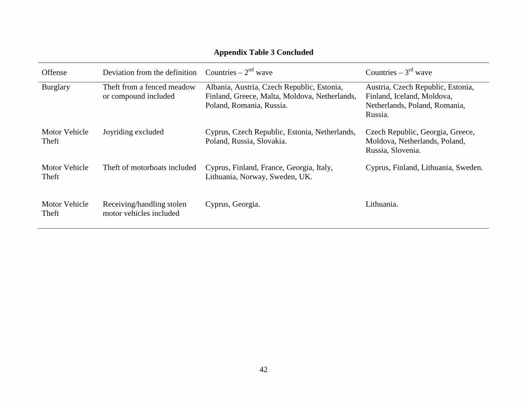
42

Appendix Table 3 Concluded

Offense Deviation from the definition Countries – 2nd wave Countries – 3rd wave

Burglary Theft from a fenced meadow or compound included

Albania, Austria, Czech Republic, Estonia, Finland, Greece, Malta, Moldova, Netherlands, Poland, Romania, Russia.

Austria, Czech Republic, Estonia, Finland, Iceland, Moldova, Netherlands, Poland, Romania, Russia.

Motor Vehicle Theft

Joyriding excluded Cyprus, Czech Republic, Estonia, Netherlands, Poland, Russia, Slovakia.

Czech Republic, Georgia, Greece, Moldova, Netherlands, Poland, Russia, Slovenia.

Motor Vehicle Theft

Theft of motorboats included Cyprus, Finland, France, Georgia, Italy, Lithuania, Norway, Sweden, UK.

Cyprus, Finland, Lithuania, Sweden.

Motor Vehicle Theft

Receiving/handling stolen motor vehicles included

Cyprus, Georgia. Lithuania.

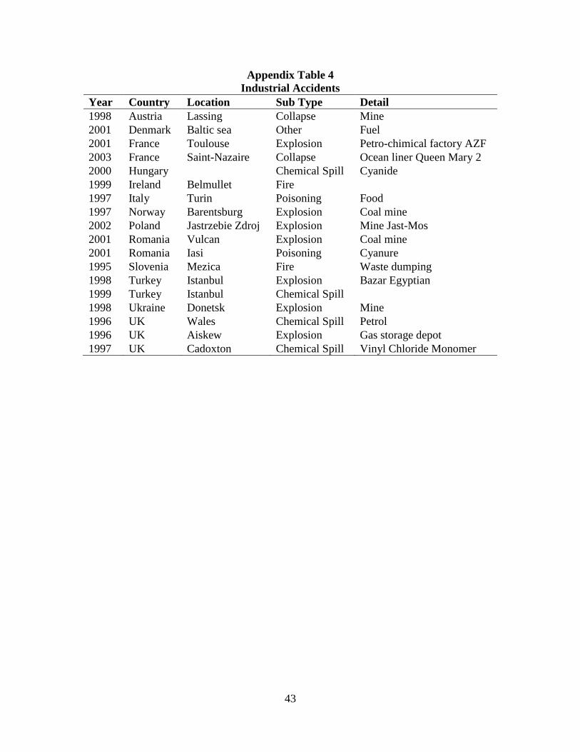
43

Appendix Table 4 Industrial Accidents

Year Country Location Sub Type Detail 1998 Austria Lassing Collapse Mine 2001 Denmark Baltic sea Other Fuel 2001 France Toulouse Explosion Petro-chimical factory AZF 2003 France Saint-Nazaire Collapse Ocean liner Queen Mary 2 2000 Hungary

Chemical Spill Cyanide

1999 Ireland Belmullet Fire 1997 Italy Turin Poisoning Food

1997 Norway Barentsburg Explosion Coal mine 2002 Poland Jastrzebie Zdroj Explosion Mine Jast-Mos 2001 Romania Vulcan Explosion Coal mine 2001 Romania Iasi Poisoning Cyanure 1995 Slovenia Mezica Fire Waste dumping 1998 Turkey Istanbul Explosion Bazar Egyptian 1999 Turkey Istanbul Chemical Spill

1998 Ukraine Donetsk Explosion Mine 1996 UK Wales Chemical Spill Petrol 1996 UK Aiskew Explosion Gas storage depot 1997 UK Cadoxton Chemical Spill Vinyl Chloride Monomer

44

Appendix Table 5 Earthquakes

Year Country Location 1998 Austria Arnoldstein 1996 Croatia Ston, Slano area 2002 Georgia Tbilisi area 1996 Greece Konitsa 1999 Greece Athens Suburbs of Menidi 2000 Greece Mihalitsi, Mitikas, Flabo 2001 Greece Aegean sea 2002 Greece Bartholomio 2003 Greece Lefkada 1997 Italy Umbria, Marche regions 1998 Italy Gualdo Tadino-Nocera 2002 Italy Sicily, Palermo 2002 Italy San Guliano di Puglia 2002 Italy Zafferana Etnea, Giarre 2003 Italy Alessandria (Piemont) 1998 Slovenia Bovec, Trenta, Kobarid 1996 Turkey Corum-Amasya 1998 Turkey Kayseri 1998 Turkey Ceyhan, Adana area 1998 Turkey Adana, Ceyhan, Hatay 1999 Turkey Duzce, Bolu, Kaynasli 1999 Turkey Sakarya Province 1999 Turkey Izmit 1999 Turkey Marmaris 1999 Turkey Kocaeli, Bursa, Istanbul 1999 Turkey Izmit, Kocaeli, Yalova

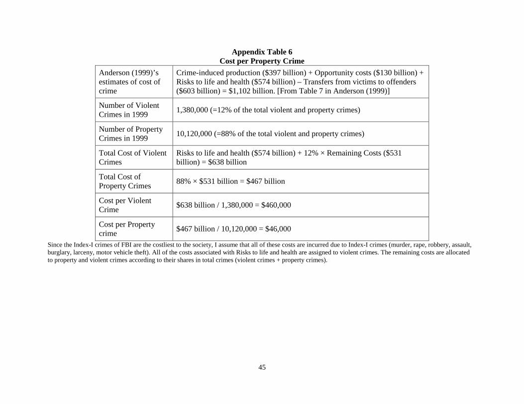
45

Appendix Table 6 Cost per Property Crime

Anderson (1999)’s estimates of cost of crime

Crime-induced production ($397 billion) + Opportunity costs ($130 billion) + Risks to life and health ($574 billion) – Transfers from victims to offenders ($603 billion) = $1,102 billion. [From Table 7 in Anderson (1999)]

Number of Violent Crimes in 1999 1,380,000 (=12% of the total violent and property crimes)

Number of Property Crimes in 1999 10,120,000 (=88% of the total violent and property crimes)

Total Cost of Violent Crimes

Risks to life and health ($574 billion) + 12% × Remaining Costs ($531 billion) = $638 billion

Total Cost of Property Crimes 88% × $531 billion = $467 billion

Cost per Violent Crime $638 billion / 1,380,000 = $460,000

Cost per Property crime $467 billion / 10,120,000 = $46,000

Since the Index-I crimes of FBI are the costliest to the society, I assume that all of these costs are incurred due to Index-I crimes (murder, rape, robbery, assault, burglary, larceny, motor vehicle theft). All of the costs associated with Risks to life and health are assigned to violent crimes. The remaining costs are allocated to property and violent crimes according to their shares in total crimes (violent crimes + property crimes).