statistical arbitrage: factor investing approach
TRANSCRIPT

Munich Personal RePEc Archive
Statistical arbitrage: Factor investing
approach
Akyildirim, Erdinc and Goncu, Ahmet and Hekimoglu, Alper
and Nguyen, Duc Khuong and Sensoy, Ahmet
University of Zurich and ETH Zurich, Switzerland, Xian
Jiaotong-Liverpool University, China, European Investment Bank,
Luxembourg, IPAG Business School, France and International
School, Vietnam National University, Vietnam, Bilkent University,
Turkey
February 2021
Online at https://mpra.ub.uni-muenchen.de/105766/
MPRA Paper No. 105766, posted 08 Feb 2021 11:10 UTC

Statistical arbitrage: Factor investing approach
Erdinc Akyildirim†, Ahmet Goncu‡, Alper Hekimoglu§,
Duc Khuong Nguyen¶k, Ahmet Sensoy
February, 2021
Abstract
We introduce a continuous time model for stock prices in a general factor represen-
tation with the noise driven by a geometric Brownian motion process. We derive the
theoretical hitting probability distribution for the long-until-barrier strategies and the
conditions for statistical arbitrage. We optimize our statistical arbitrage strategies
with respect to the expected discounted returns and the Sharpe ratio. Bootstrapping
results show that the theoretical hitting probability distribution is a realistic represen-
tation of the empirical hitting probabilities. We test the empirical performance of the
long-until-barrier strategies using US equities and demonstrate that our trading rules
can generate statistical arbitrage profits.
Keywords: Statistical arbitrage; factor models; trading strategies; geometric Brownian
motion; Monte Carlo simulation.
JEL: G11, G12, G17University of Zurich, Zurich, Switzerland ([email protected])†ETH Zurich, Zurich, Switzerland‡Xian Jiaotong-Liverpool University, Suzhou, China ([email protected])§European Investment Bank, Luxembourg ([email protected])¶Corresponding author. IPAG Business School, Paris, France ([email protected])kInternational School, Vietnam National University, Hanoi, Vietnam
Bilkent University, Ankara, Turkey ([email protected])
1

1 Introduction
Statistical arbitrage strategies emerge from the widely used pairs trading strategy which
dates back to 1980s. In pairs trading, it is assumed that there exist two stocks with similar
characteristics, which are highly correlated after removing the effects of the common risk
factors. Pairs trading exploits market overreaction to new information and whenever the
co-integration residual between the two assets is larger than its statistical equilibrium level,
the investor shorts the relatively more expensive asset while taking a long position in the
cheaper asset (see Elliott et al. (2005) for details on pairs trading). Accordingly, most of
the statistical arbitrage trading strategies exploit relative mispricing of assets based on the
long-run statistical equilibrium levels or trading signals, and they often require data mining,
advanced information technology infrastructure, and trading speed.
In the literature, the existence of statistical arbitrage opportunities refers to a riskless
profit opportunity as time or number of trades goes to infinity. Avellaneda and Lee (2010)
state that the trading strategies that exploit these opportunities have three common features
as follows: (i) trading signals are systematic or rule based, (ii) trading book is market-neutral,
and (iii) the mechanism for generating excess returns is statistical. Authors use this definition
on US equities to analyse the empirical performance of model driven statistical arbitrage
strategies. On the other hand, Hogan et al. (2004) provide a mathematical definition of
statistical arbitrage which is used in testing the existence of statistical arbitrage opportunities
in US equity markets. Later, Jarrow et al. (2012) revise this definition to relax the variance
condition of statistical arbitrage proposed by Hogan et al. (2004).
Amongst others, examples of empirical studies on the performance of statistical arbitrage
strategies are given by Elliott et al. (2005), Gatev et al. (2006), Do and Faff (2010), Avel-
laneda and Lee (2010) Cummins and Bucca (2012), Huck and Afawubo (2015). With the
accumulation of big data and availability of necessary infrastructure for the high frequency
trading, it also became possible to investigate statistical arbitrage in these environments
(Stubinger et al., 2018; Stubinger and Endres, 2018; Stubinger, 2019; Nasekin and Hardle,
2
2019). Recently, there are also machine learning approaches developed to exploit the statis-
tical arbitrage opportunities in different financial markets (Krauss et al., 2017; Knoll et al.,
2019; Huck, 2019). Most of the empirical studies conclude that stock prices appear to con-
tradict the efficient market hypothesis, where excess returns are obtained consistently with
the trading signals based on the publicly available information.
In this study, instead of comparing various trading strategies in terms of their excess
returns, we show under what conditions statistical arbitrage exists and how it can be ex-
ploited in an optimal way. Optimal statistical arbitrage trading for Ito diffusion processes
and Ornstein-Uhlenbeck processes are studied by Bertram (2010) and Bertram (2009), re-
spectively. However, these studies do not consider the existence issue with a mathematical
definition of statistical arbitrage. One of the few mathematical definitions of statistical
arbitrage is given by Bondarenko (2003). In this study, author derives a martingale type no-
statistical arbitrage restriction assuming that financial derivatives are traded in the market.
Goncu (2015) proves the existence of statistical arbitrage in the Black-Scholes framework via
trading strategies that consist of holding an over-performing stock until it hits a deterministic
barrier, whereas Goncu and Akyildirim (2017) extend these results for the multi-asset Black-
Scholes framework. Focardi et al. (2016) introduce a statistical arbitrage strategy based on
dynamic factor models of prices and empirically test it on US equities. Their results show
that prices allow for significantly more accurate forecasts than returns in their model and
their strategy passes the test for statistical arbitrage.1
In our study, we decompose asset returns in a general factor model framework which is
similar to the factor model representation given by Avellaneda and Lee (2010). Our main
contributions to the literature are as follows. First, we derive the statistical arbitrage con-
dition in the factor model framework which is written in terms of the stock drift, volatility,
and factor betas. Based on this condition, the trader decides the implementation of a long-
until-barrier strategy. We show that the statistical arbitrage strategies utilized in this work
1For other noteworthy studies, see Mayordomo et al. (2014); Jarrow et al. (2019); Lutkebohmert andSester (2020).
3

satisfy the definitions of statistical arbitrage given by Hogan et al. (2004) and Avellaneda
and Lee (2010). Second, we derive the theoretical hitting probabilities of the stock prices to
the deterministic barrier levels in the factor model. Based on the hitting probabilities, we
also derive optimal trading rules based on two types of objective functions, i.e., (i) maximiz-
ing the discounted expected trading profits, or (ii) maximizing a Sharpe ratio type objective
function. Then, we compare the empirical hitting probabilities with the theoretical distribu-
tion derived via bootstrapping experiments. Third, we conduct Monte Carlo simulations to
verify the convergence of the simulated hitting time probabilities to the theoretical hitting
time distribution for the time-dependent barrier levels. We also perform bootstrapping ex-
periments to verify the theoretical and empirical hitting probabilities. In this vein, statistical
arbitrage trading strategies are implemented with the stock return data from the US mar-
ket to check the empirical power of these strategies in terms of out-of-sample performance.
Finally, as a robustness, we apply White (2000)’s reality check to test for any potential data
snooping bias in the trading strategies considered.
The statistical arbitrage condition we derive for the factor model allows the trader to
optimize her/his trading strategy given her/his beliefs about the drift, volatility, and factor
loading of the stock or the portfolio. It is important to note that we are not suggesting
a method to forecast the future values of these parameters. Each investor might have a
different estimate of the physical measure of the stock price returns, and thus, they specu-
late in the market. As in our empirical examples, the historical estimates obtained from an
expanding in-sample estimation window might serve quite well to check the statistical arbi-
trage condition and generate statistical arbitrage profits. Furthermore, since the existence of
our statistical arbitrage condition depends on an inequality, the precision of the parameter
estimation does not need to be high as long as the direction of the inequality is estimated
correctly.
The motivation for employing the factor model framework is its effectiveness in explaining
stock returns, simplicity, and wide-spread use in the financial industry. Analytical tractabil-
4
ity of the factor-based model enables us to derive analytical formulas for the hitting time
distribution of the stock price for deterministic barriers. Furthermore, factor models are often
used for risk management and performance evaluation of portfolio managers. Our statistical
arbitrage methodology can be applied to sector or industry exchange traded funds (ETFs)
with a relative value market neutral strategy by a long position in an investor’s favourite
sector ETF combined with a short position in a less attractive sector ETF. Amongst many
choices of factor models in the literature, we employ the well-known Fama and French (1993)
three factor model for our empirical examples. However, we are not constrained by the choice
of this factor model and our framework applies to any other factor model as well. Another
advantage of the factor models is that the estimation of the correlation matrix for thousands
of assets is very difficult compared to finding or modelling the correlation between factors
that explain the stock returns. Furthermore, when the information explained by the factors
are extracted, the idiosyncratic noise in each asset is much closer to normality, which is
consistent with the use of Brownian motion for log-returns.
The rest of this article is organized as follows. Section 2 explains the the stock price
process in a general factor model. Section 3 presents our statistical arbitrage strategies with
the derivation of the statistical arbitrage condition and shows that our statistical arbitrage
strategies satisfy the definition by Avellaneda and Lee (2010). It also derives the optimal
statistical arbitrage trading rules with respect to two alternative objective functions with
possible constraints. Section 4 includes a variety of empirical and simulated experiments
verifying the theoretical results. Monte Carlo experiments are conducted to verify the con-
vergence of the simulated hitting probabilities to the derived theoretical hitting distribution
of the stock prices for the deterministic barriers, whereas bootstrapping experiments are
employed to verify the empirical hitting probabilities and the theoretical probabilities. Fur-
thermore, empirical performance of the statistical arbitrage long-until-barrier strategy is also
tested with the US equity market data. Finally, Section 5 concludes the article.
5

2 Statistical Arbitrage and Stock Price Model
Within our proposed framework, we utilize the following mathematical definition of sta-
tistical arbitrage as given by Hogan et al. (2004), but later we also show that our statistical
arbitrage strategies satisfy the definition given by Avellaneda and Lee (2010) as well. Given
the stochastic process v(t) : t 0 for the discounted cumulative trading profits, which is
defined on a probability space (Ω,F , P ), the statistical arbitrage is defined as follows (Hogan
et al., 2004):
Definition 1 A statistical arbitrage is a zero initial cost, self-financing trading strategy
v(t) : t 0 with cumulative discounted value v(t) such that
1. v(0) = 0
2. limt!1 E[v(t)] > 0,
3. limt!1 P (v(t) < 0) = 0, and
4. limt!1 var(v(t))/t = 0 if P (v(t) < 0) > 0, 8t < 1.
It is clear that a standard arbitrage opportunity is a special case of statistical arbitrage. A
standard arbitrage strategy V has V (0) = 0 (self-financing) with a finite time T such that
P (V (t) > 0) > 0 and P (V (t) 0) = 1 for t T and the proceeds of this profit can be
deposited into money market account for the rest of the infinite time horizon.
With regards to our stock price model, let F jt := F j
0 + jWjF (t) for j = 1, 2, .., p be
our factor processes where W 1F ,W
2F , ...,W
pF are independent Brownian motions and j is the
volatility for the factor process F jt . We define our factor based stock price process such that
it is based on the time averaged value of the integrated factors defined above,
St = exp
ln(S0) + (↵ 2/2)t+1
t
pX
j=1
j
Z t
0
F js ds+ WS(t)
!
, j = 1, 2, .., p, (1)
6

where WS and W jF are independent Brownian motions from each other for all j = 1, .., p.
Plugging in the definition of the factor process into the above equation, we obtain the
following stock price model with a regular Brownian motion process
St = exp
ln(S0) + (↵ 2/2)t+
pX
j=1
jFj0 +
1
t
pX
j=1
j
Z t
0
jWjF (s)ds+ WS(t)
!
, j = 1, 2, .., p,
(2)
wherePp
j=1 j
R t
0jW
jF (s)ds N
0,Pp
j=1
2j
2j t
3
3
. Hence, we obtain
St = exp
0
@ln(S0) + (↵ 2/2)t+
pX
j=1
jFj0 +
vuut
pX
j=1
2j
2j
3+ 2
!
W (t)
1
A , j = 1, 2, .., p,
(3)
where W (t) is a convoluted Brownian motion. Moreover, following definitions of the first
two moments of St will be useful further.
E (St) = exp
(↵ +1
6
pX
j=1
2j
2j )T +
pX
j=1
jFj0
!
(4)
V (St) = exp
2
↵ + 2 +
Ppj=1 j
2j
3
!
T +
pX
j=1
jFj0
!
(5)
exp
2↵ +
Ppj=1 j
2j
3
!
T + 2
pX
j=1
jFj0
!
Next, we define the following first passage time problem:
= inft : t 0, St S0(1 + k)erf t
(6)
where k is a constant which determines the barrier level together with the risk free rate rf .
Using the stock price process given in equation (3), we can rewrite the above problem as
= inf
0
@t : t 0,
↵ 1
22 rf
t+
pX
j=1
jFj0 +
0
@
sPp
j=1 2j
2j
3+ 2
1
AW (t) log(1 + k)
1
A (7)
7

Next, by using the analytical formulas given by Shreve (2004) for the first passage time
density of the Brownian motion, we can write the density for the discounted stock price in
the time averaged factor model as follows
p(t 2 dt) =log(1 + k)
Pp
j=1 jFj0
r
2Pp
j=1 2j
2j + 2
t3exp
0
B@
log(1 + k)Pp
j=1 jFj0 ↵ + rf + 2/2
2
2Pp
j=1 2j
2j
3+ 2
t
1
CA (8)
This gives us the hitting probability of the stock price to the barrier level as follows:
P ( t) = Φ
(↵ rf 2/2)tMp
Nt
+exp
2(↵ rf 2/2)M
N
Φ
(↵ + rf + 2/2)tMp
Nt
(9)
where
M = ln(1 + k)pX
j=1
jFj0 , (10)
N =
Ppj=1
2j
2j
3+ 2, (11)
and Φ is the cumulative distribution function for the normal distribution.
3 Statistical Arbitrage Strategy
We first start with a strategy that fails to satisfy the statistical arbitrage in Definition 1.
A simple buy-and-hold strategy is shown to fail the conditions of statistical arbitrage due to
the exponential growth of the variance of discounted cumulative profits over time whereas
long-until-barrier strategies are shown to satisfy the statistical arbitrage conditions. The
key in proving the statistical arbitrage conditions is to utilize a barrier level that grows
proportional to the risk free rate and to show the finite first passage time to such boundaries.
8

Therefore, by deriving the first passage time distribution under the factor model framework,
we are able to design a statistical arbitrage strategy with almost sure finite first passage
to the deterministic boundary that guarantees positive profit. The existence of statistical
arbitrage is given with respect to certain conditions on the model parameters. Next, we
discuss the buy-and-hold strategy.
3.1 Buy-and-Hold Strategy
The variance term derived in equation (5) shows that for ↵ > rf , buy-and-hold strategies
fail to yield statistical arbitrage since limt!1 var(v(t))/t = 1 and there is always a positive
probability of loss (see Proposition 2 by Goncu (2015) for details). Buy-and-hold strategy
fails to satisfy the Definition 1 since we are not able to control the variance as time increases.
To be able to control the variance of the trading profits, we need to reduce the risky asset
holding in our portfolio as time increases. Therefore, we introduce a barrier or termination
condition to sell the risky asset held and invest all the proceeds in the risk-free account.
3.2 Long-Until-Barrier Strategy
Since the buy-and-hold strategy fails to satisfy the definition of statistical arbitrage, we
define a deterministic barrier level S0(1+k)erf t for the risky asset to sell it whenever its price
reaches this level. This deterministic barrier grows proportional to the risk-free rate, which
guarantees the positivity of the discounted trading profits whenever we close the position in
the risky asset. However, in order to show the existence of statistical arbitrage in the sense
of Definition 1, we need the finite first passage time of the underlying stochastic process to
reach this barrier level.
The discounted cumulative trading profits from this strategy is given by
v(t) =
8
>><
>>:
S0k if k 2 [0, t],
Sterf t S0 else ,
(12)
9

where the first passage time to the barrier is given in equation (6).
As proved in the previous section, for defined in equation (6), if the drift term satis-
fies µ = ↵ 2
2+Pp
j=1 Fj0 > 0, then the first passage time of the stock price process to
the boundary given by S0erf t(1 + k) is guaranteed to be finite and the first passage time
distribution is given in equation (9).
Generating statistical arbitrage profits thus boils down to having a good guess about the
above condition. The finiteness of the first passage time to the barrier level implies that the
variance and the probability of loss in our trading strategy will decay to zero for sufficiently
large time t.
3.3 Optimal Barrier (Filter Rule)
The statistical arbitrage condition shows that as long as we have accurate estimation of
the model parameters of asset prices, there exists statistical arbitrage opportunities in the
economy. In this section, our goal is to find the optimal barrier level or in other words, the
optimal limit order level for each time t that maximizes the expected profits or Sharpe ratio
in a statistical arbitrage trading. Given the estimates or beliefs about the future alpha (↵)
and volatility of the stock, we find the optimal level k to buy/sell each risky asset in a
portfolio. First, we start the with the maximization of the expected profits:
maxk
E[v(T )] = maxk
E[v(T )|k < T ]P (k < T ) + E[v(T )|k T ]P (k T ) (13)
= maxk
(
kS0(1 P (k > T )) +
P (k > T )S0
exp
↵ rf +1
6
pX
j=1
2j
2j
!
T +
pX
j=1
jFj0
!
1
!)
10

The first order condition for the optimization is
@E[v(T )]/@k = S0(P (k < T )) + (14)
S0@P (k > T )
@k
exp
(↵ rf +1
6
pX
j=1
2j
2j )T +
pX
j=1
jFj0
!
1 k
!
= 0,
where the optimal k is the root of the non-linear equation (14). We can further rewrite
equation (14) in a more compact form,
@E[v(T )]/@k =@ ((k C)F (k) + C)
@k
= (k C)@F (k)
@k+ F (k)
= k +F (k)
F 0(k) C = 0 (15)
where F (k) refers to equation (9) and
C = exp
↵ rf +1
6
pX
j=1
2j
2j
!
T +
pX
j=1
jFj0
!
1
Clearly, we can find the optimal k by finding the roots of the above equation. By using
the cumulative distribution function for the first passage time density, equation (15) can be
written as
k +Φ (A) + e(ln(1+k)
Ppj=1 jF
j0 )Φ (B)
1(k+1)
h(A)
+ e(ln(1+k)Pp
j=1 jFj0 )
Φ (B) 1pt (B)
i + C = 0
11

where
A =(α− rf −
1
2σ2)t− ln(1 + k) +
Pp
j=1βjF
j0
σ√
t, (16)
B =(−α + rf +
1
2σ2)t− ln(1 + k) +
Pp
j=1βjF
j0
σ√
t,
γ = 2
α− rf −1
2σ2
,
σs =
v
u
u
t
Pp
j=1β2jσ
2j
3+ σ2
!
.
Our second method to find the optimal k is the optimization of Sharpe ratio which can be
defined as
maxk
ST = maxk
E[v(T )]
E[p
var(v(T ))](17)
To compute the above ratio, we need the variance of the cumulative profits v(t). Hence,
E[var(v(T ))] = var(v(T )|τk > T )P (τk > T ) + 0P (τk < T ) ,
and by using our stock model definition in equation (3), we obtain
E[p
var(v(T ))] = S0
v
u
u
u
t
0
@e2
α−rf+σ2+
Ppj=1
βjσ2j
3
!
T+Pp
j=1βjF
j0
− 1
1
AP (τk > T ) + 0P (τk < T ).
This finally leads to
maxk
ST = maxk
S0 (k − C)F (k) + C
S0
v
u
u
u
t
0
@e2
α−rf+σ2+
Ppj=1
βjσ2j
3
!
T+Pp
j=1βjF
j0
− 1
1
A (1− F (k))
, (18)
12

and the first order condition is derived as
1
C
F 0(k) (F (k) (k C) + C)
(1 F (k))3/2+
F 0(k) (1 F (k)) (k C) + F (k) (1 F (k))
F 0(k) (1 F (k))
!
= 0 (19)
where C =
vuuut
0
@e2
↵rf+2+
Ppj=1
βjσ2j
3
!
T+Pp
j=1 jFj0 1
1
A
After some tedious algebra we finally obtain:
kF 0(k) + F (k) F (k)2 = 0 =) k =F (k)2 F (k)
F 0(k)(20)
3.4 Monte Carlo Experiments
In this section, we discuss the Monte Carlo experiments utilized to verify our theoretical
results. Namely, we check whether the hitting probability distribution implied by the pro-
posed model and its parameters are numerically correct or not. Moreover, we use this exact
distribution to further generate optimal barrier parameter k using our different approaches.
Therefore, the precision of the theoretical results are of importance in this verification.
The simulation of the maximum of Brownian motion is not a trivial process and depends
on the simulation of Brownian motion paths. Here we provide a useful derivation which
helps us to simulate this maximum in an efficient way. Using the conditional distribution
for the maximum of Brownian motion together with the given Brownian motion path, we
can simulate the maximum value attained over a fixed time period. As explained by Shreve
(2004), we start by writing the conditional distribution of Brownian motion and its maximum
as follows
13
fM(t)|W (t)(m|w) =fM(t),W (t)(m,w)
fW (t)(w)
=2(2m w)
tp2t
p2te
(2m−w)2
2t+w2
2t
=2(2m w)
te
−2m(m−w)t
Using this conditional density, one can derive the maximum process as
P (Mt m|W (t) = w) =
Z m
w
2(2u w)
te
−2u(u−w)t du = 1 e
−2m(m−w)t
Given that any inverse cumulative distribution function is uniformly distributed, we can
start by simulating the uniform distribution and continue by inverse transformation method:
1 e−2m(m−w)
t = U
2m2 + 2mw
t= 1 ln(U)
2m2 2mw + t(1 ln(U)) = 2m2 2mw + C = 0
where C = t(1 ln(U)). This is a standard quadratic function hence it is trivial to find the
roots as
∆ = 4w2 8C,
m1,2 =2w ±
p∆
4(21)
Then using the positive root from the above formula, we can obtain the maximum of Brow-
nian motion. This exact solution for the roots of maximum process will help us to simulate
the maximum of the Brownian motion without using any numerical root finding algorithm.
The summary of our methodology can be outlined as follows,
14

(i) Simulate a Brownian motion path,
(ii) Simulate uniform random variable U(0, 1),
(iii) Then use equation (21) to find the roots m1 & m2 and select the positive root as the
simulated maximum value.
Using the procedure above, we generate the exact simulation of max(St) and obtain more
precise and efficient Monte Carlo results without resorting to fully discretized path simulation
which can be computationally more expensive. Therefore, at each time point tk, we simulate
the following
Stk = S0 exp
0
@(↵ 2/2)tk +
pX
j=1
jFj0 +
vuut
pX
j=1
2j
2j
3+ 2
!
tkMtk
1
A (22)
where Mtk = max(Wtk)|Wtk and Wtk =ptkZk where Zk is a standard normal random
variable. The parameters that are used in the simulation exercise are given in Table 1.
Insert Table 1 about here
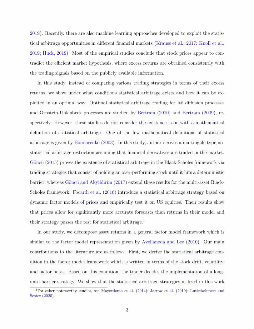
From Figure 1, we observe that the Monte Carlo procedure works well and the error is
quite low with even 10,000 simulations. These results verify that the simulated hitting time
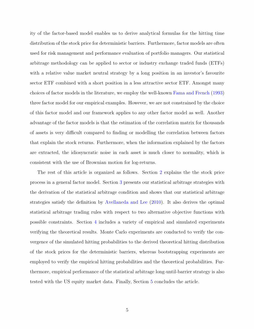
probabilities converge to the theoretical hitting time probabilities. We also conduct Monte
Carlo simulations to test our theoretical results given by equations (4) and (5). In Figure
2, we observe the average trading profits, time averaged variance and the probability of loss
for the buy-and-hold strategy. As it is consistent with our theoretical results, both mean
and time average of variance go to infinity as time increases. However, if we repeat the
same experiment for different investment horizons by introducing a barrier in the trading
strategy, from Figure 3 it is clear that time average variance decays to zero which in turn
yields statistical arbitrage.
15
Insert Figures 1 & 2 & 3 about here
4 Empirical Analysis
This section describes the dataset that we use in the empirical testing of our theoretical
results together with the estimation methodology to find the parameters for our factor based
stock price model. We also present the results of the bootstrapping experiments (see Section
4.3) comparing the theoretical hitting probabilities with the empirical hitting probabilities
of the long-until-barrier type strategies with different investment horizons. Finally, long-
until-barrier type strategies are back-tested in terms of out-of-sample performance for the
optimal barrier levels that we derived earlier (see Section 4.4).
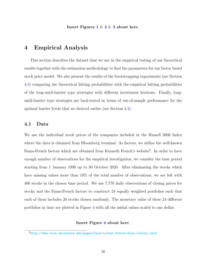
4.1 Data
We use the individual stock prices of the companies included in the Russell 3000 Index
where the data is obtained from Bloomberg terminal. As factors, we utilize the well-known
Fama-French factors which are obtained from Kenneth French’s website2. In order to have
enough number of observations for the empirical investigation, we consider the time period
starting from 1 January 1990 up to 30 October 2020. After eliminating the stocks which
have missing values more than 10% of the total number of observations, we are left with
480 stocks in the chosen time period. We use 7,770 daily observations of closing prices for
stocks and the Fama-French factors to construct 24 equally weighted portfolios such that
each of them includes 20 stocks chosen randomly. The monetary value of these 24 different
portfolios in time are plotted in Figure 4 with all the initial values scaled to one dollar.
Insert Figure 4 about here
2http://mba.tuck.dartmouth.edu/pages/faculty/ken.french/data_library.html
16

We see that all the portfolios suffer significant drawdown in three periods during the 1990
to 2020 period. The first major drawdown is observed during the 2001 dotcom bubble burst.
The second market crash happened during and after the 2008 subprime mortgage crisis,
whereas the last one is due to the global Covid-19 pandemic causing extreme downturns
in the stock markets. Therefore, the sample period gives us sufficiently rich scenarios for
testing the statistical arbitrage strategies and hitting probabilities not only during normal
market conditions but also during market crashes.
Insert Table 2 about here
With regards to pricing factors, we employ the Fama-French three factor model where
the factors are denoted by SMB (Small Minus Big), HML (High Minus Low), and Rm Rf
(market excess return over the risk-free rate). The descriptive statistics for the log-returns
of the equally weighted portfolios are given in Table 2. From this table, we observe that
the maximum (minimum) value of 0.00035 (0.00017) for the mean of the daily log-returns
is attained by the Portfolio 13 (7) which corresponds to around 8.82% (4.24%) in annual
terms. It is also clear from the table that there is not much variation across the portfolios
in terms of the daily fluctuations which on average corresponds to about 20% annualized
volatility. The daily loss/profit values across the portfolios range from as low as around -16%
up to 13% during the time period investigated. As mentioned before, it is important to note
that the time period includes both 2001 and 2008 financial crises and the economic crash
due to Covid-19 pandemic which are all worse than the great depression in terms of loss in
market value. All portfolios have negative skewness, meaning that the left side tail of the
log-returns distribution is longer or fatter than the right side of the distribution. Similarly,
all the portfolios have kurtosis greater than three which indicates that the distributions have
heavier tails than normal distribution because of the extreme events in the sample period.
17

4.2 Estimation
In order to estimate the parameters of our base model given in equation (1), we first
express the factors in an equivalent representation using the Ito’s lemma. For any factor j,
we have the following:
j
Z t
0
F j(s)ds = j
F j0 t+ j
Z t
0
W jF (s)ds
= j
F j0 t+W j
F (t)t j
Z t
0
sdW jF (s)
Then, using the stock price model in equation (1), we obtain:
log (St) = log (S0) +
↵ 2
2
t+
pX
j=1
j
t
Z t
0
F j(s)ds
+ WS(t)
= log (S0) +
↵ 2
2
t+
pX
j=1
0
B@jF
j0 + jjW
jF (t)
| z
jF j(t)
1
CA
pX
j=1
jj
t
Z t
0
sdW jF (s)
+ WS(t)
| z
(t)
Based on this representation, we obtain logarithmic returns through discretization:
log
St
St∆t
=
↵ 2
2
∆t+
pX
j=1
j∆F jt +∆(t)
| z
t
(23)
where t N
0,∆tPp
j=1 2j
2j
3
1 2∆t
3t
+ 2
. For large values of t, the variance of the
residuals t is equal to ∆tPp
j=1 2j
2j
3+ 2
.
Then, the regression equation can be written as
rt = a+
pX
j=1
jfjt + t (24)
18

where a =
↵ 2
2
∆t, rt = log
St
St−∆t
and F jt is the log of the factor, and thus, f j
t := ∆F jt
becomes the factor log-returns.
From the linear regression in equation (24) and setting the time increments to daily time
horizon, we obtain the model parameters. First, the factor coefficients j’s are obtained from
the regression formula, then we obtain the remaining parameters ↵ and as
2 =
1
T
TX
t=1
2t =
pX
j=1
2j
2j
3
1 2
3t
+ 2
=) 2 =1
T
TX
t=1
2t pX
j=1
2j
2j
3
1 2
3t
(25)
Using this result, we proceed to write ↵ as
↵ = a+2
2(26)
where ↵, a, are sample estimates of ↵, a, . The volatility of each factor is obtained from
the sample standard deviation over the considered sample of factors.
4.3 Bootstrapping
Theoretical hitting probability distribution derived in equation (9) is tested via bootstrapping
experiments. The main idea of bootstrapping follows selecting random subsamples of the
complete dataset and comparing the theoretical hitting probability obtained from equation
(9) with the actual hitting times of different portfolios of stocks over time. The theoretical
hitting probabilities can be calculated for a given barrier level k and time horizon T . The
inverse problem can be formulated as the calculation of the barrier level for a given holding
period T and probability of hitting the barrier before time T . Therefore, in order to work
with fixed probability events over random subsamples with fixed lengths, we vary the barrier
level k accordingly across different portfolios of assets and over time. Therefore, we do not
need to change the time span of each random subsample and probability, but instead use
19

different implied barrier levels in each bootstrapping subsample.
We briefly summarize the bootstrapping procedure. We start by selecting random block
of subsample of observations where the asset is held for T number of days to verify if the
barrier is reached or not. By repeating the frequency count of the number of hits relative to
the number of subsamples tested, we obtain the empirical probability of hitting the barrier
for a given level of fixed probability and corresponding barrier level k. In other words, the
bootstrapping procedure repeatedly selects a random starting point in time to check if the
barrier is reached for a fixed time period and fixed probability while the corresponding k
is calculated each time. For each subsample, the parameters are estimated by equation
(24) and solving for the original model parameters. For example, if the first subsample is
starting at the trading day 1,000, then we utilize all the past information to estimated model
parameters up to day 1,000. Depending on the holding period, we check if the barrier is
reached in the next T trading days or not. In the bootstrapping process, the subsampling
is repeated for 300 times. By counting the ratio of barrier hits out of 300 trials, we obtain
the estimate for the empirical hitting probability at different theoretical probability levels
for given holding periods. Note that the barrier level k is calculated for a given time horizon
and probability level. Bootstrapping is repeated for 24 different portfolios for different time
horizons and different probability levels.
In Figure 5, we consider four different holding periods given as 20, 40, 60 and 80 business
days and results are presented for theoretical hitting probabilities of 0.5, 0.6, 0.7, 0.8 and
0.9. Theoretical probabilities are given along the line, whereas the empirical probabilities
obtained from the hitting ratios are given for 24 different portfolios. It is often observed
that the empirical hitting ratios are relatively more likely than the theoretical probabilities.
The normality of the noise term in the stock price model in equation (1) is not a perfect
assumption to capture the properties of stock price returns. However, it allows for ana-
lytical tractability in the derivation of theoretical hitting density for long-until-barrier type
strategies. Therefore, the bootstrapping exercise reveals the fact that asset returns exhibit
20

jumps.
Insert Figure 5 about here
In Figure 5, lower probability levels such as at the 0.5 or 0.6 level, we observe relative
larger difference between the empirical hitting probability versus the theoretical probabilities.
In Tables 3-6, the empirical and theoretical probabilities are given for each portfolio and the
corresponding barrier level k with different holding periods. Each portfolio has different set
of parameters for the given sample of observations until the start date of the investment in
the stock. Therefore, for each portfolio we calculate the barrier level k that gives us the same
probability for the given holding period. From the Tables 3-6, it can be verified that the
implied k levels that yield the fixed probability levels are stable across different portfolios
with the average implied k values presented in the columns next to the empirical probability
obtained from 300 randomly bootstrapped subsamples.
Insert Tables 3 & 4 & 5 & 6 about here
It can be observed that the empirical versus theoretical probabilities show similar behavior
with larger differences at the lower probability levels. Note that lower probabilities such as 0.5
or 0.6 correspond to larger barrier level k and thus with the excess kurtosis of stock returns,
it is not surprising to observe a higher difference for larger barrier levels. Empirical hitting
ratios are higher than the theoretical rates and this shows that the likelihood of obtaining
the statistical arbitrage is higher than what the model assumes. Therefore, bootstrapping
results verify that the theoretical hitting distribution of the stock prices to the barrier level
is a conservative approximation to the empirical hitting probabilities.
4.4 Backtesting the Statistical Arbitrage Strategies
In Section 3, we have given the statistical arbitrage condition for the long-until-barrier
strategy and now, we verify the empirical performance of long-until-barrier strategies with
21

the same 24 portfolios of stocks used in the bootstrapping method. For this purpose, we
consider the long-until-barrier strategy with the optimal barrier levels calculated from the
expected return and Sharpe ratio maximization given in equations (16) and (20), respectively.
In doing so, the first 200 observations are utilized as the initial in sample portion for
the empirical backtesting. Parameters of the model are estimated dynamically with all
the available past information up to the current trading day. For example, when a long
position is opened on day i, all the previous data up to day i is used for the parameter
estimation. Based on the estimated parameters, optimal barrier levels k are calculated from
the expected return and Sharpe ratio maximization. Similar to the bootstrapping method,
out-of-sample backtesting experiments are conducted for 20, 40, 60, and 80 holding days. The
investor has the choice of implementing the long-until-barrier strategy at different investment
horizons. However, if the investor has a short investment horizon then this strategy should
be backtested with a higher frequency dataset instead of the daily price data.
In our framework, reasonable holding periods can be in the order of months. Holding
periods that are too short would not be suitable for testing with the daily data, whereas
very long holding periods would imply very few instances of the stock price process reaching
the barrier levels empirically. Most importantly, the critical parameter is the trend of the
stock price process. If the trend is expected to remain bullish for the near future, then
the long-until-barrier strategy would perform and achieve its target price and the position
is closed. On the other hand, if the investment horizon is much longer, the barrier level
should be re-calculated daily with the re-calibrated parameters on a daily basis as well. In
our backtesting methodology, an expanding window is utilized and we estimate the model
parameters using all the data available until the date we open the long position and do
not re-calibrate model parameters during the maximum holding period of 20, 40, 60, and 80
days, respectively. Once the trader opens a long position, we allow for the position to remain
open up until three times the investment horizon. If the stock price still does not reach the
barrier level by the maximum waiting period then the position is closed at the close price
22

by the end of the maximum waiting period.
If the trader has the target holding period of 20 days implementing the long-until-barrier
strategy, he opens the position at the closing price of the trading day i and is allowed to
wait at most three times the 20 days, i.e. 60 trading days, to reach the barrier to close the
position. At the end of the 60 days, the position is closed if the barrier level is not reached
yet.
In Table 7, for all portfolios, we present the average returns arising from the out-of-sample
backtesting with barrier levels obtained from the expected return maximization algorithm. In
Table 8, the out-of-sample backtesting results from the Sharpe ratio maximization algorithm
are given. It can be seen that in terms of the average performance across portfolios, barrier
levels that optimize expected return and Sharpe ratio to perform indistinguishably similar.
It should also be noted that we are using the closing prices in the backtesting methodology
and it is possible that such a selection can cause an underestimation of the profitability of
the strategy since the highest prices attained intraday are higher than the closing prices with
more frequent realizations of the target profit levels. The smoother performance of the equal
weighted statistical arbitrage strategies shows that by implementing such strategies across
different portfolios or assets would also reduce the probability of loss due to unexpected
changes in the trends of assets.
Insert Tables 7 & 8 about here
In Figures 6 and 7, we provide the histograms of the trading profits for the equally
weighted statistical arbitrage trading strategies for the out-of-sample period with respect to
different investment horizons. In Figure 6, the histogram is given for the statistical arbitrage
strategy with the barrier levels derived from the expected return maximization, whereas in
Figure 7, the barriers level are obtained from the Sharpe ratio optimization method.
Insert Figures 6 & 7 about here
23

Overall, the performance of the statistical arbitrage strategies are better at the 80-days
investment horizon both with the expected return or Sharpe ratio maximizing barrier levels.
For this investment horizon, we reach to an average annualized return of 11% with an annual
volatility of 33%. The maximum drawdown in all the strategies are low, showing that such
strategies can be implemented over diversified portfolios of assets as long as the trend of the
asset remains the same over the short investment horizons.
4.5 Testing for Data Snooping Bias
Statistical arbitrage trading strategies should be tested for the existence of data snooping
bias. In particular, trading strategies that utilize the long-until-barrier strategies might suffer
from the data snooping effects due to potential biases in the considered time period. Trading
scenarios that study the performance of general trading strategies end up with too many
combinations or trading rules that produce a wide range of performance results. However,
by using expected return and Sharpe ratio maximization methods for the selection of the
optimal barrier levels as two main alternatives for the implementation of the trading strategy,
we obtain only two types of trading strategies that is applied in the same way for all the
wide range of random portfolios constructed. Therefore, our methodology is not expected to
suffer from data snooping bias due to its standardized methodology for the implementation
of trading strategies. In any case, we control for potential data snooping bias over different
sample periods and with new datasets.
Due to the convention in testing trading strategies, White (2000)’s reality check is applied
to verify for any potential data snooping bias in our trading strategies. We test the null
hypothesis which states that the maximum average return of the trading rules being tested
is same as the average return of the benchmark, against the alternative that the maximum
average return of the trading rules is greater than the average return of the benchmark. The
data mining test is employed on the daily return series obtained from the implementation
of the long-until-barrier type trading strategies. Four different bootstrap block sizes are
24

considered, namely 20, 40, 60 and 80 business days of block sub-sampling. As each size of
the robustness test, the bootstrapping method is implemented on 500 replications.
Insert Tables 9 about here
In Table 9, the p-values obtained from the White’s reality check are given for the expected
return and Sharpe ratio maximization strategies, respectively. The findings show that our
results do not suffer from data snooping bias since the majority of the portfolios have p-
values less than %10. Especially, we observe that the p-values decrease significantly for the
Sharpe ratio optimization with increasing holding periods.
5 Conclusion
In this article, we introduce a factor model framework for the statistical arbitrage strate-
gies. Within this framework, we derive the the hitting probability distribution of the stock
prices to deterministic barrier levels. Furthermore, Monte Carlo simulations are utilized to
verify the theoretical probabilities of the hitting time distribution derived. Derivation of the
hitting time distribution of the stock price process to the barrier level is crucial in order to
prove the existence of a statistical arbitrage strategy. Although the factor model framework
offers us analytical tractability in the derivation of the hitting time distribution of the stock
prices to a deterministic barrier level, it has its own limitations. The major limitation is the
normality assumption of the noise term of the factor model representation. This assumption
reflects itself as the underestimation of the empirical hitting probabilities in comparison to
the theoretical hitting time distribution derived. This implies that the likelihood of reaching
and obtaining the target profit levels in the long-until-barrier strategies is higher compared
to the model assumptions as long as the trend of the stock price process remains positive.
Bootstrapping exercises are implemented to verify the behavior of the empirical hitting time
probabilities versus the theoretical probabilities from the distribution function derived.
25

Next, we derive the condition (in terms of the drift, volatility, and factor loadings of the
stock price process) that guarantees the existence of the statistical arbitrage. As the second
step, we consider alternative methods to obtain best barrier level by optimizing different
objective functions. Optimal statistical arbitrage trading strategies are derived based on the
probability of hitting a deterministic barrier level to terminate the strategy. We derive the
optimal barrier levels to close the long positions for a given investment horizon based on the
expected discounted profit, or alternatively, with respect to the Sharpe ratio maximization.
Finally, we apply backtesting to verify the out-of-sample performance of long-until-barrier
type strategies across a wide range of portfolios of assets in the US equity market. Results
show that although the definition of statistical arbitrage depends on the information on the
future values of the model parameters, with relatively short holding periods, most of the
time barrier levels are reached and the investor can lock in the excess return. This is simply
because during the sample period, we observe overall positive drift and trend in the portfolios
with the exception of two major financial turmoil periods. It is also natural that statistical
arbitrage strategies introduced in our theoretical framework are not perfect and they also
show higher drawdown during unexpected market crashes. However, with the use of intraday
data, such strategies can be modified to control for drawdown at intraday holding periods
and accompanying stop-loss levels can be introduced for designing trading strategies that
can handle the market risk better.
References
Avellaneda, M., Lee, J.H., 2010. Statistical arbitrage in the us equities market. Quantitative
Finance 10, 761–782.
Bertram, W.K., 2009. Optimal trading strategies for Ito diffusion processes. Physica A:
Statistical Mechanics and its Applications 388, 2865–2873.
26

Bertram, W.K., 2010. Analytical solutions for optimal statistical arbitrage trading. Physica
A: Statistical Mechanics and its Applications 389, 2234–2243.
Bondarenko, O., 2003. Statistical arbitrage and securities prices. Review of Financial Studies
16, 875–919.
Cummins, M., Bucca, A., 2012. Quantitative spread trading on crude oil and refined products
markets. Quantitative Finance 12, 1857–1875.
Do, B., Faff, R., 2010. Does simple pairs trading still work? Financial Analysts Journal 66,
83–95.
Elliott, R.J., Van Der Hoek, J., Malcolm, W.P., 2005. Pairs trading. Quantitative Finance
5, 271–276.
Fama, E.F., French, K.R., 1993. Common risk factors in the returns on stocks and bonds.
Journal of Financial Economics 33, 3–56.
Focardi, S.M., Fabozzi, F.J., Mitov, I.K., 2016. A new approach to statistical arbitrage:
Strategies based on dynamic factor models of prices and their performance. Journal of
Banking and Finance 65, 134–155.
Gatev, E., Goetzmann, W.N., Rouwenhorst, K.G., 2006. Pairs trading: Performance of a
relative-value arbitrage rule. Review of Financial Studies 19, 797–827.
Goncu, A., 2015. Statistical arbitrage in the black–scholes framework. Quantitative Finance
15, 1489–1499.
Goncu, A., Akyildirim, E., 2017. Statistical arbitrage in the multi-asset black–scholes econ-
omy. Annals of Financial Economics 12, 1750004.
Hogan, S., Jarrow, R., Teo, M., Warachka, M., 2004. Testing market efficiency using statis-
tical arbitrage with applications to momentum and value strategies. Journal of Financial
Economics 73, 525–565.
27

Huck, N., 2019. Large data sets and machine learning: Applications to statistical arbitrage.
European Journal of Operational Research 278, 330–342.
Huck, N., Afawubo, K., 2015. Pairs trading and selection methods: is cointegration superior?
Applied Economics 47, 599–613.
Jarrow, R., Li, H., Ye, X., Hu, M., 2019. Exploring mispricing in the term structure of CDS
spreads. Review of Finance 23, 161–198.
Jarrow, R., Teo, M., Tse, Y.K., Warachka, M., 2012. An improved test for statistical
arbitrage. Journal of Financial Markets 15, 47–80.
Knoll, J., Stubinger, J., Grottke, M., 2019. Exploiting social media with higher-order fac-
torization machines: Statistical arbitrage on high-frequency data of the S&P 500. Quan-
titative Finance 19, 571–585.
Krauss, C., Do, X.A., Huck, N., 2017. Deep neural networks, gradient-boosted trees, random
forests: Statistical arbitrage on the S&P 500. European Journal of Operational Research
259, 689–702.
Lutkebohmert, E., Sester, J., 2020. Robust statistical arbitrage strategies. Quantitative
Finance (forthcoming).
Mayordomo, S., Pena, J.I., Romo, J., 2014. Testing for statistical arbitrage in credit deriva-
tives markets. Journal of Empirical Finance 26, 59–75.
Nasekin, S., Hardle, W.K., 2019. Model-driven statistical arbitrage on letf option markets.
Quantitative Finance 19, 1817–1837.
Shreve, S.E., 2004. Stochastic Calculus for Finance II: Continuous-Time Models. Springer-
Verlag, New York.
Stubinger, J., 2019. Statistical arbitrage with optimal causal paths on high-frequency data
of the S&P 500. Quantitative Finance 19, 921–935.
28
Stubinger, J., Endres, S., 2018. Pairs trading with a mean-reverting jump–diffusion model
on high-frequency data. Quantitative Finance 18, 1735–1751.
Stubinger, J., Mangold, B., Krauss, C., 2018. Statistical arbitrage with vine copulas. Quan-
titative Finance 18, 1831–1849.
White, H., 2000. A reality check for data snooping. Econometrica 68, 1097–1126.
29

Figure 1: Convergence of empirical hitting probabilities to the theoretical hitting probabili-ties derived in the hitting time distribution.
0 5 10 15 20 25 30
Holding Period
0.4
0.5
0.6
0.7
0.8
0.9
1# of Simulations: 100 Avg.MC error: -0.03017
theoretical
Monte Carlo
0 5 10 15 20 25 30
Holding Period
0.4
0.5
0.6
0.7
0.8
0.9
1# of Simulations: 1000 Avg.MC error: 0.01583
theoretical
Monte Carlo
0 5 10 15 20 25 30
Holding Period
0.4
0.5
0.6
0.7
0.8
0.9
1# of Simulations: 10000 Avg.MC error: 0.0056299
theoretical
Monte Carlo
0 5 10 15 20 25 30
Holding Period
0.4
0.5
0.6
0.7
0.8
0.9
1# of Simulations: 100000 Avg.MC error: 0.00028993
theoretical
Monte Carlo
30

Figure 2: Evolution of mean, time averaged variance and probability of loss for the buy-and-hold strategy. Investment horizons considered: 1, 2, 5, 10, 20, 50 years.
10 20 30 40 50 60 70
Holding Period
20
40
60
80
100
120
PnLbuyhold
E(PnL) T->
10 20 30 40 50 60 70
Holding Period
0.15
0.2
0.25
0.3
0.35
Prob.of Loss
P(Loss) T->
10 20 30 40 50 60 70
Holding Period
0.5
1
1.5
2
2.5
Vola
tility
104 Var(PnLbuyhold) T->
31

Figure 3: Evolution of mean, time averaged variance and probability of loss for the long-until-barrier strategy. Investment horizons considered: 1, 2, 5, 10, 20, 50 years.
10 20 30 40 50 60 70
Holding Period
0.08
0.1
0.12
0.14
0.16
0.18
PnL
E(PnL) T->
10 20 30 40 50 60 70
Holding Period
0.02
0.04
0.06
0.08
0.1
0.12
0.14
0.16
Prob.of Loss
P(Loss) T->
10 20 30 40 50 60 70
Holding Period
0.005
0.01
0.015
0.02
0.025
Vola
tility
Var(PnL) T->
32

Figure 4: The price series of twenty four stock portfolios in the time period from 1/1/1990to 30/10/2020 with all the initial prices scaled to one dollar.
33

Figure 5: Empirical hitting probabilities of 24 portfolios to the barrier level for a givenholding period of 20-, 40-, 60-, 80-days compared to theoretical probabilities.
0.5 0.55 0.6 0.65 0.7 0.75 0.8 0.85 0.90.5
0.6
0.7
0.8
0.9T= 20 days
theoretical
empirical
0.5 0.55 0.6 0.65 0.7 0.75 0.8 0.85 0.90.5
0.6
0.7
0.8
0.9
1T= 40 days
theoretical
empirical
0.5 0.55 0.6 0.65 0.7 0.75 0.8 0.85 0.90.5
0.6
0.7
0.8
0.9
1T= 60 days
theoretical
empirical
0.5 0.55 0.6 0.65 0.7 0.75 0.8 0.85 0.90.5
0.6
0.7
0.8
0.9
1T= 80 days
theoretical
empirical
34

Figure 6: Out-of-sample performance of the long-until-barrier strategies using the optimalbarrier levels from expected return maximization where each position is held for differentinvestment horizons of 20-, 40-, 60-, and 80-days, respectively. The out-of-sample test periodis divided into time periods with given investment horizons.
-0.5 -0.4 -0.3 -0.2 -0.1 0 0.1 0.2
0
20
40
60
80
10020 days
-0.6 -0.5 -0.4 -0.3 -0.2 -0.1 0 0.1 0.2 0.3
0
10
20
30
4040 days
-0.5 -0.4 -0.3 -0.2 -0.1 0 0.1 0.2 0.3
0
5
10
15
20
2560 days
-0.6 -0.5 -0.4 -0.3 -0.2 -0.1 0 0.1 0.2 0.3 0.4
0
5
10
15
2080 days
35

Figure 7: Out-of-sample performance of the long-until-barrier strategies using the optimalbarrier levels from Sharpe ratio maximization where each position is held for different in-vestment horizons of 20-, 40-, 60-, and 80-days, respectively. The out-of-sample test periodis divided into time periods with given investment horizons.
-0.5 -0.4 -0.3 -0.2 -0.1 0 0.1 0.2 0.3 0.4
0
20
40
60
80
100
12020 days
-0.6 -0.4 -0.2 0 0.2 0.4 0.6
0
10
20
30
40
5040 days
-0.5 -0.4 -0.3 -0.2 -0.1 0 0.1 0.2 0.3 0.4
0
5
10
15
20
25
3060 days
-0.6 -0.4 -0.2 0 0.2 0.4 0.6 0.8
0
5
10
15
20
2580 days
36

Table 1: Parameters considered throughout the Monte Carlo experiments.
Stock parameters 0.0002↵ 0.0774
Factor parametersRm Rf SMB HML
j 0.1254 0.0725 0.0644j 1.0960 0.4270 0.2300F0 -0.0016 -0.0126 0.0210
Table 2: Descriptive statistics for the daily-log returns of the equally weighted portfolios ofRussell 3000 stocks for the period 01 Jan 1990 to 30 Oct 2020. P-i refers to i-th portfolio.
mean median std min max skewness kurtosisP-1 0.00027 0.00059 0.013 -0.150 0.130 -0.592 16.333P-2 0.00021 0.00058 0.012 -0.145 0.117 -0.589 15.309P-3 0.00021 0.00059 0.013 -0.146 0.096 -0.799 14.284P-4 0.00026 0.00053 0.011 -0.136 0.106 -0.517 18.605P-5 0.00031 0.00045 0.012 -0.136 0.104 -0.694 16.758P-6 0.00019 0.00050 0.012 -0.143 0.086 -0.690 14.074P-7 0.00017 0.00048 0.013 -0.140 0.089 -0.599 11.902P-8 0.00025 0.00059 0.014 -0.126 0.113 -0.508 13.754P-9 0.00029 0.00059 0.013 -0.138 0.100 -0.630 14.073P-10 0.00022 0.00053 0.013 -0.124 0.088 -0.690 13.256P-11 0.00034 0.00064 0.012 -0.120 0.092 -0.414 13.140P-12 0.00032 0.00069 0.013 -0.108 0.097 -0.494 12.091P-13 0.00035 0.00073 0.013 -0.168 0.111 -0.730 15.627P-14 0.00021 0.00052 0.012 -0.120 0.103 -0.613 16.095P-15 0.00028 0.00048 0.013 -0.155 0.092 -0.546 14.144P-16 0.00025 0.00065 0.012 -0.135 0.103 -0.718 15.510P-17 0.00020 0.00060 0.014 -0.151 0.097 -0.639 13.624P-18 0.00027 0.00075 0.013 -0.136 0.097 -0.510 12.739P-19 0.00031 0.00053 0.012 -0.128 0.123 -0.396 15.769P-20 0.00025 0.00076 0.013 -0.137 0.112 -0.636 15.083P-21 0.00025 0.00047 0.012 -0.119 0.106 -0.454 13.021P-22 0.00030 0.00065 0.012 -0.117 0.122 -0.368 16.631P-23 0.00030 0.00056 0.012 -0.134 0.110 -0.757 15.801P-24 0.00026 0.00059 0.014 -0.131 0.111 -0.405 11.203
average 0.00026 0.00058 0.013 -0.135 0.104 -0.583 14.534
37

Table 3: Empirical hitting probabilities of 24 portfolios together with the correspondingbarrier levels k for a holding period of T= 20 days. theoretical probability (tp), empiricalprobability (ep), implied k (impK). P-i refers to i-th portfolio.
tp = 0.5 tp = 0.6 tp = 0.7 tp = 0.8 tp = 0.9ep impK ep impK ep impK ep impK ep impK
P-1 0.58 0.017 0.61 0.013 0.71 0.010 0.75 0.007 0.83 0.004P-2 0.57 0.019 0.63 0.015 0.68 0.011 0.77 0.008 0.86 0.005P-3 0.56 0.016 0.62 0.013 0.69 0.009 0.78 0.006 0.85 0.004P-4 0.58 0.020 0.65 0.015 0.75 0.011 0.78 0.008 0.85 0.004P-5 0.57 0.021 0.64 0.016 0.68 0.012 0.78 0.008 0.83 0.005P-6 0.58 0.022 0.67 0.017 0.72 0.012 0.77 0.008 0.82 0.005P-7 0.63 0.021 0.69 0.016 0.77 0.012 0.79 0.008 0.83 0.005P-8 0.60 0.020 0.65 0.015 0.69 0.011 0.75 0.008 0.82 0.005P-9 0.63 0.018 0.67 0.014 0.80 0.010 0.84 0.007 0.86 0.004P-10 0.59 0.020 0.65 0.015 0.73 0.011 0.81 0.008 0.85 0.004P-11 0.61 0.019 0.71 0.014 0.76 0.011 0.85 0.007 0.86 0.005P-12 0.62 0.019 0.71 0.015 0.78 0.011 0.79 0.008 0.83 0.005P-13 0.62 0.017 0.68 0.013 0.75 0.010 0.81 0.007 0.85 0.004P-14 0.67 0.020 0.71 0.015 0.74 0.011 0.78 0.008 0.83 0.005P-15 0.67 0.018 0.75 0.014 0.76 0.010 0.81 0.007 0.82 0.004P-16 0.54 0.021 0.63 0.016 0.70 0.012 0.74 0.008 0.80 0.005P-17 0.65 0.019 0.70 0.014 0.74 0.011 0.79 0.007 0.87 0.005P-18 0.61 0.018 0.65 0.014 0.74 0.010 0.78 0.007 0.85 0.004P-19 0.58 0.021 0.65 0.017 0.73 0.012 0.80 0.008 0.87 0.005P-20 0.57 0.017 0.65 0.013 0.71 0.010 0.79 0.007 0.85 0.004P-21 0.60 0.017 0.66 0.013 0.74 0.010 0.80 0.007 0.87 0.004P-22 0.50 0.021 0.59 0.016 0.66 0.012 0.72 0.008 0.79 0.005P-23 0.62 0.019 0.72 0.015 0.76 0.011 0.82 0.008 0.85 0.005P-24 0.69 0.018 0.76 0.014 0.79 0.011 0.85 0.007 0.86 0.005average 0.60 0.019 0.67 0.015 0.73 0.011 0.79 0.007 0.84 0.004
38

Table 4: Empirical hitting probabilities of 24 portfolios together with the correspondingbarrier levels k for a holding period of T= 40 days. theoretical probability (tp), empiricalprobability (ep), implied k (impK). P-i refers to i-th portfolio.
tp = 0.5 tp = 0.6 tp = 0.7 tp = 0.8 tp = 0.9ep impK ep impK ep impK ep impK ep impK
P-1 0.66 0.025 0.70 0.019 0.76 0.014 0.83 0.009 0.88 0.005P-2 0.68 0.027 0.72 0.021 0.76 0.015 0.81 0.010 0.92 0.006P-3 0.63 0.023 0.72 0.018 0.76 0.013 0.84 0.009 0.89 0.005P-4 0.70 0.028 0.74 0.022 0.83 0.016 0.89 0.011 0.90 0.006P-5 0.68 0.029 0.74 0.023 0.80 0.017 0.86 0.011 0.91 0.006P-6 0.64 0.032 0.70 0.024 0.79 0.018 0.88 0.012 0.93 0.006P-7 0.76 0.030 0.78 0.023 0.84 0.017 0.89 0.011 0.93 0.006P-8 0.65 0.028 0.71 0.022 0.80 0.016 0.82 0.010 0.89 0.006P-9 0.69 0.026 0.75 0.020 0.79 0.014 0.87 0.010 0.90 0.006P-10 0.64 0.028 0.76 0.022 0.80 0.016 0.87 0.010 0.91 0.006P-11 0.74 0.026 0.77 0.020 0.79 0.015 0.87 0.010 0.95 0.006P-12 0.69 0.027 0.77 0.021 0.82 0.015 0.87 0.010 0.89 0.006P-13 0.68 0.024 0.75 0.019 0.81 0.014 0.89 0.009 0.93 0.005P-14 0.70 0.028 0.76 0.022 0.84 0.016 0.86 0.011 0.92 0.006P-15 0.75 0.026 0.81 0.020 0.87 0.015 0.88 0.010 0.89 0.005P-16 0.60 0.031 0.66 0.024 0.72 0.017 0.77 0.011 0.84 0.006P-17 0.63 0.027 0.74 0.021 0.81 0.015 0.86 0.010 0.90 0.006P-18 0.73 0.026 0.79 0.020 0.82 0.015 0.90 0.010 0.93 0.005P-19 0.60 0.030 0.70 0.023 0.76 0.017 0.85 0.011 0.91 0.006P-20 0.60 0.024 0.70 0.019 0.76 0.014 0.82 0.009 0.90 0.005P-21 0.66 0.024 0.76 0.018 0.84 0.013 0.87 0.009 0.90 0.005P-22 0.53 0.030 0.63 0.023 0.74 0.017 0.82 0.011 0.85 0.006P-23 0.68 0.027 0.74 0.021 0.81 0.015 0.85 0.010 0.92 0.006P-24 0.73 0.026 0.78 0.020 0.85 0.015 0.90 0.010 0.93 0.006average 0.67 0.027 0.74 0.021 0.80 0.015 0.86 0.010 0.91 0.006
39

Table 5: Empirical hitting probabilities of 24 portfolios together with the correspondingbarrier levels k for a holding period of T= 60 days. theoretical probability (tp), empiricalprobability (ep), implied k (impK). P-i refers to i-th portfolio.
tp = 0.5 tp = 0.6 tp = 0.7 tp = 0.8 tp = 0.9ep impK ep impK ep impK ep impK ep impK
P-1 0.63 0.031 0.69 0.024 0.75 0.017 0.81 0.011 0.88 0.006P-2 0.62 0.034 0.75 0.026 0.79 0.019 0.81 0.012 0.93 0.007P-3 0.65 0.029 0.72 0.022 0.78 0.016 0.84 0.011 0.90 0.006P-4 0.70 0.035 0.76 0.027 0.81 0.020 0.87 0.013 0.91 0.007P-5 0.66 0.036 0.74 0.028 0.84 0.020 0.89 0.013 0.91 0.007P-6 0.63 0.039 0.69 0.030 0.75 0.022 0.86 0.014 0.94 0.007P-7 0.79 0.037 0.83 0.029 0.87 0.021 0.90 0.014 0.94 0.007P-8 0.65 0.034 0.73 0.027 0.79 0.019 0.87 0.013 0.89 0.007P-9 0.66 0.032 0.75 0.024 0.79 0.018 0.83 0.012 0.91 0.006P-10 0.61 0.035 0.74 0.027 0.85 0.019 0.90 0.013 0.93 0.007P-11 0.77 0.033 0.85 0.025 0.86 0.018 0.89 0.012 0.94 0.007P-12 0.67 0.034 0.75 0.026 0.80 0.019 0.88 0.012 0.88 0.007P-13 0.67 0.030 0.72 0.023 0.81 0.017 0.88 0.011 0.93 0.006P-14 0.65 0.035 0.74 0.027 0.84 0.020 0.86 0.013 0.92 0.007P-15 0.73 0.032 0.79 0.024 0.88 0.018 0.89 0.012 0.92 0.006P-16 0.64 0.038 0.66 0.029 0.73 0.021 0.79 0.014 0.83 0.007P-17 0.67 0.033 0.73 0.025 0.82 0.018 0.84 0.012 0.91 0.007P-18 0.67 0.032 0.78 0.025 0.85 0.018 0.92 0.012 0.96 0.006P-19 0.60 0.038 0.67 0.029 0.76 0.021 0.85 0.014 0.92 0.007P-20 0.64 0.030 0.71 0.023 0.76 0.017 0.82 0.011 0.90 0.006P-21 0.70 0.029 0.72 0.022 0.80 0.016 0.89 0.011 0.91 0.006P-22 0.52 0.037 0.59 0.029 0.72 0.021 0.82 0.014 0.89 0.007P-23 0.63 0.034 0.69 0.026 0.79 0.019 0.86 0.012 0.91 0.007P-24 0.74 0.032 0.80 0.025 0.86 0.018 0.91 0.012 0.94 0.007average 0.66 0.034 0.73 0.026 0.80 0.019 0.86 0.012 0.91 0.007
40
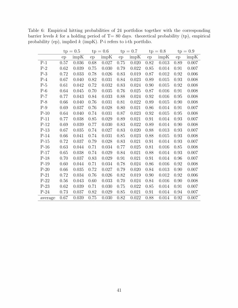
Table 6: Empirical hitting probabilities of 24 portfolios together with the correspondingbarrier levels k for a holding period of T= 80 days. theoretical probability (tp), empiricalprobability (ep), implied k (impK). P-i refers to i-th portfolio.
tp = 0.5 tp = 0.6 tp = 0.7 tp = 0.8 tp = 0.9ep impK ep impK ep impK ep impK ep impK
P-1 0.57 0.036 0.68 0.027 0.75 0.020 0.82 0.013 0.89 0.007P-2 0.62 0.039 0.75 0.030 0.79 0.022 0.85 0.014 0.91 0.007P-3 0.72 0.033 0.78 0.026 0.83 0.019 0.87 0.012 0.92 0.006P-4 0.67 0.040 0.82 0.031 0.84 0.023 0.89 0.015 0.93 0.008P-5 0.61 0.042 0.72 0.032 0.83 0.024 0.90 0.015 0.92 0.008P-6 0.64 0.045 0.70 0.035 0.76 0.025 0.87 0.016 0.91 0.008P-7 0.77 0.043 0.84 0.033 0.88 0.024 0.92 0.016 0.95 0.008P-8 0.66 0.040 0.76 0.031 0.81 0.022 0.89 0.015 0.90 0.008P-9 0.69 0.037 0.76 0.028 0.80 0.021 0.86 0.014 0.91 0.007P-10 0.64 0.040 0.74 0.031 0.87 0.023 0.92 0.015 0.95 0.008P-11 0.77 0.038 0.85 0.029 0.89 0.021 0.91 0.014 0.93 0.007P-12 0.69 0.039 0.77 0.030 0.83 0.022 0.89 0.014 0.90 0.008P-13 0.67 0.035 0.74 0.027 0.83 0.020 0.88 0.013 0.93 0.007P-14 0.66 0.041 0.74 0.031 0.85 0.023 0.88 0.015 0.93 0.008P-15 0.72 0.037 0.79 0.028 0.83 0.021 0.91 0.014 0.93 0.007P-16 0.63 0.044 0.71 0.034 0.77 0.025 0.81 0.016 0.85 0.008P-17 0.65 0.038 0.74 0.029 0.84 0.021 0.88 0.014 0.93 0.007P-18 0.70 0.037 0.83 0.029 0.91 0.021 0.91 0.014 0.96 0.007P-19 0.60 0.044 0.71 0.034 0.78 0.024 0.86 0.016 0.92 0.008P-20 0.66 0.035 0.72 0.027 0.79 0.020 0.84 0.013 0.90 0.007P-21 0.72 0.034 0.76 0.026 0.82 0.019 0.90 0.012 0.92 0.006P-22 0.56 0.043 0.60 0.033 0.70 0.024 0.84 0.016 0.90 0.008P-23 0.62 0.039 0.71 0.030 0.75 0.022 0.85 0.014 0.91 0.007P-24 0.73 0.037 0.82 0.029 0.85 0.021 0.91 0.014 0.94 0.007average 0.67 0.039 0.75 0.030 0.82 0.022 0.88 0.014 0.92 0.007
41

Table 7: The out-of-sample backtesting results from the expected return maximization algorithm for the target holding periodof 20-, 40-, 60-, 80- days. P-i refers to i-th portfolio. Rets (Vol) stands for the annualized returns (volatility). MaxDD is themaximum drawdown.
20-days 40-days 60-days 80-daysRets Vol Sharpe MaxDD Rets Vol Sharpe MaxDD Rets Vol Sharpe MaxDD Rets Vol Sharpe MaxDD
P-1 0.11 0.25 0.18 0.25 0.09 0.24 0.24 0.25 0.10 0.21 0.34 0.25 0.13 0.37 0.35 0.23P-2 0.07 0.22 0.14 0.23 0.07 0.22 0.19 0.23 0.08 0.22 0.26 0.23 0.10 0.28 0.29 0.23P-3 0.09 0.26 0.15 0.22 0.08 0.24 0.20 0.22 0.09 0.23 0.27 0.22 0.14 0.47 0.27 0.21P-4 0.09 0.17 0.23 0.22 0.09 0.17 0.30 0.22 0.09 0.17 0.40 0.22 0.09 0.17 0.45 0.22P-5 0.13 0.23 0.24 0.22 0.11 0.21 0.33 0.22 0.12 0.19 0.46 0.22 0.15 0.32 0.48 0.22P-6 0.08 0.23 0.15 0.21 0.07 0.21 0.20 0.21 0.07 0.27 0.27 0.21 0.14 0.41 0.25 0.21P-7 0.08 0.27 0.12 0.21 0.06 0.25 0.15 0.21 0.07 0.25 0.20 0.21 0.16 0.62 0.20 0.18P-8 0.13 0.31 0.18 0.21 0.09 0.27 0.21 0.21 0.10 0.29 0.31 0.21 0.18 0.52 0.30 0.20P-9 0.12 0.29 0.18 0.22 0.10 0.27 0.23 0.22 0.10 0.25 0.30 0.22 0.15 0.46 0.31 0.21P-10 0.09 0.26 0.15 0.20 0.08 0.25 0.18 0.20 0.09 0.23 0.26 0.20 0.10 0.38 0.26 0.19P-11 0.11 0.18 0.29 0.19 0.13 0.18 0.40 0.19 0.13 0.18 0.54 0.19 0.20 0.31 0.50 0.19P-12 0.12 0.23 0.23 0.19 0.12 0.23 0.31 0.19 0.13 0.24 0.42 0.19 0.17 0.38 0.43 0.19P-13 0.15 0.28 0.23 0.25 0.13 0.26 0.30 0.25 0.14 0.25 0.41 0.25 0.20 0.46 0.41 0.25P-14 0.10 0.22 0.18 0.20 0.08 0.20 0.24 0.20 0.09 0.19 0.33 0.20 0.09 0.21 0.39 0.20P-15 0.13 0.28 0.19 0.23 0.10 0.23 0.27 0.23 0.12 0.23 0.37 0.23 0.19 0.42 0.36 0.23P-16 0.10 0.23 0.19 0.22 0.09 0.22 0.24 0.22 0.10 0.22 0.34 0.22 0.13 0.31 0.38 0.21P-17 0.10 0.28 0.14 0.23 0.08 0.26 0.18 0.23 0.09 0.32 0.27 0.23 0.13 0.48 0.23 0.22P-18 0.10 0.25 0.18 0.21 0.10 0.23 0.25 0.21 0.10 0.23 0.32 0.21 0.14 0.38 0.35 0.21P-19 0.11 0.21 0.23 0.22 0.12 0.23 0.30 0.22 0.12 0.21 0.43 0.22 0.15 0.27 0.44 0.20P-20 0.10 0.24 0.18 0.22 0.10 0.24 0.25 0.22 0.11 0.31 0.33 0.22 0.16 0.45 0.31 0.21P-21 0.10 0.22 0.20 0.20 0.10 0.22 0.28 0.20 0.09 0.20 0.34 0.20 0.10 0.22 0.39 0.19P-22 0.12 0.21 0.24 0.21 0.12 0.22 0.32 0.21 0.11 0.18 0.46 0.21 0.12 0.21 0.51 0.21P-23 0.12 0.20 0.25 0.22 0.11 0.21 0.34 0.22 0.11 0.19 0.45 0.22 0.23 0.40 0.45 0.20P-24 0.11 0.29 0.15 0.22 0.10 0.28 0.20 0.22 0.10 0.28 0.28 0.22 0.13 0.46 0.27 0.19
42

Table 8: The out-of-sample backtesting results from the Sharpe ratio maximization algorithm for the target holding period of20-, 40-, 60-, 80- days. P-i refers to i-th portfolio. Rets (Vol) stands for the annualized returns (volatility). MaxDD is themaximum drawdown.
20-days 40-days 60-days 80-daysRets Vol Sharpe MaxDD Rets Vol Sharpe MaxDD Rets Vol Sharpe MaxDD Rets Vol Sharpe MaxDD
P-1 0.11 0.25 0.18 0.25 0.08 0.23 0.22 0.25 0.11 0.23 0.34 0.23 0.13 0.37 0.44 0.23P-2 0.07 0.22 0.13 0.23 0.07 0.23 0.16 0.23 0.08 0.21 0.27 0.23 0.09 0.35 0.26 0.23P-3 0.09 0.26 0.15 0.22 0.07 0.25 0.16 0.22 0.08 0.25 0.21 0.22 0.10 0.49 0.24 0.21P-4 0.09 0.18 0.21 0.22 0.09 0.19 0.28 0.22 0.09 0.17 0.38 0.22 0.09 0.19 0.39 0.22P-5 0.11 0.22 0.23 0.22 0.11 0.22 0.30 0.22 0.12 0.20 0.42 0.22 0.13 0.32 0.44 0.22P-6 0.08 0.23 0.15 0.21 0.06 0.22 0.17 0.21 0.09 0.25 0.29 0.21 0.09 0.48 0.27 0.21P-7 0.05 0.27 0.08 0.21 0.05 0.27 0.10 0.21 0.06 0.26 0.15 0.21 0.09 0.69 0.21 0.21P-8 0.11 0.28 0.17 0.21 0.09 0.27 0.19 0.21 0.12 0.32 0.29 0.21 0.15 0.67 0.32 0.21P-9 0.10 0.28 0.16 0.22 0.10 0.30 0.19 0.22 0.10 0.26 0.24 0.22 0.14 0.54 0.29 0.22P-10 0.09 0.27 0.13 0.20 0.08 0.26 0.17 0.20 0.08 0.24 0.24 0.20 0.08 0.41 0.23 0.19P-11 0.13 0.19 0.29 0.19 0.13 0.19 0.39 0.19 0.13 0.18 0.50 0.19 0.15 0.29 0.55 0.17P-12 0.12 0.24 0.21 0.19 0.12 0.23 0.29 0.19 0.11 0.22 0.36 0.19 0.13 0.40 0.40 0.19P-13 0.13 0.27 0.20 0.25 0.12 0.26 0.25 0.25 0.12 0.24 0.35 0.25 0.18 0.45 0.46 0.25P-14 0.09 0.23 0.17 0.20 0.07 0.22 0.19 0.20 0.08 0.21 0.27 0.20 0.09 0.23 0.33 0.20P-15 0.12 0.27 0.18 0.23 0.10 0.25 0.22 0.23 0.11 0.24 0.31 0.23 0.14 0.46 0.41 0.23P-16 0.10 0.24 0.18 0.22 0.09 0.24 0.22 0.22 0.10 0.22 0.29 0.22 0.12 0.35 0.36 0.21P-17 0.07 0.26 0.12 0.23 0.07 0.26 0.16 0.23 0.11 0.31 0.27 0.23 0.16 0.77 0.28 0.22P-18 0.10 0.26 0.17 0.21 0.09 0.25 0.21 0.21 0.11 0.24 0.29 0.21 0.13 0.39 0.35 0.21P-19 0.11 0.21 0.23 0.22 0.10 0.21 0.27 0.22 0.10 0.20 0.35 0.22 0.11 0.33 0.37 0.20P-20 0.09 0.25 0.16 0.22 0.09 0.25 0.23 0.22 0.10 0.25 0.31 0.22 0.14 0.52 0.39 0.22P-21 0.10 0.23 0.19 0.20 0.08 0.21 0.23 0.20 0.10 0.21 0.31 0.20 0.10 0.24 0.34 0.19P-22 0.12 0.22 0.24 0.21 0.11 0.21 0.30 0.21 0.12 0.18 0.47 0.21 0.13 0.23 0.51 0.21P-23 0.13 0.22 0.25 0.22 0.11 0.21 0.29 0.22 0.12 0.20 0.43 0.20 0.13 0.29 0.49 0.20P-24 0.09 0.29 0.13 0.22 0.08 0.28 0.18 0.22 0.10 0.29 0.26 0.20 0.13 0.66 0.28 0.20
43

Table 9: Probability values coming from the White’s reality check for the expected return and Sharpe ratio maximizationalgorithms are given for the 20-, 40-, 60-, and 80- days holding periods, respectively. P-i refers to i-th portfolio.
Expected Return Sharpe Ratio20-days 40-days 60-days 80-days 20-days 40-days 60-days 80-days
P-1 0.044 0.014 0.024 0.028 0.028 0.026 0.038 0.036P-2 0.122 0.078 0.092 0.122 0.144 0.092 0.048 0.066P-3 0.110 0.078 0.094 0.124 0.118 0.092 0.110 0.080P-4 0.012 0.008 0.012 0.014 0.018 0.002 0.008 0.006P-5 0.006 0.006 0.010 0.002 0.012 0.002 0.008 0.004P-6 0.102 0.082 0.104 0.124 0.116 0.068 0.046 0.036P-7 0.270 0.238 0.270 0.308 0.422 0.342 0.340 0.300P-8 0.064 0.048 0.080 0.076 0.084 0.046 0.054 0.102P-9 0.092 0.088 0.072 0.066 0.110 0.062 0.064 0.058P-10 0.148 0.138 0.102 0.154 0.192 0.160 0.124 0.144P-11 0.000 0.000 0.004 0.002 0.002 0.000 0.000 0.000P-12 0.004 0.008 0.010 0.010 0.022 0.010 0.014 0.006P-13 0.018 0.008 0.012 0.008 0.042 0.024 0.028 0.002P-14 0.024 0.016 0.024 0.032 0.046 0.034 0.012 0.028P-15 0.038 0.044 0.028 0.038 0.048 0.036 0.060 0.042P-16 0.026 0.022 0.014 0.010 0.038 0.022 0.032 0.018P-17 0.110 0.144 0.134 0.128 0.162 0.118 0.052 0.020P-18 0.056 0.036 0.048 0.028 0.066 0.066 0.092 0.044P-19 0.008 0.002 0.008 0.008 0.006 0.012 0.008 0.000P-20 0.084 0.074 0.050 0.084 0.182 0.102 0.102 0.028P-21 0.058 0.036 0.040 0.026 0.046 0.036 0.020 0.024P-22 0.000 0.002 0.004 0.000 0.004 0.002 0.000 0.000P-23 0.002 0.004 0.002 0.008 0.000 0.000 0.000 0.002P-24 0.116 0.146 0.144 0.142 0.196 0.182 0.102 0.052
44