Marquette Universitye-Publications@Marquette

Master's Theses (2009 -) Dissertations, Theses, and Professional Projects

Factor Based Statistical Arbitrage in the U.S. EquityMarket with a Model Breakdown DetectionProcessSeoungbyung parkMarquette University

Recommended Citationpark, Seoungbyung, "Factor Based Statistical Arbitrage in the U.S. Equity Market with a Model Breakdown Detection Process" (2017).Master's Theses (2009 -). 419.http://epublications.marquette.edu/theses_open/419

i

FACTOR BASED STATISTICAL ARBITRAGE IN THE U.S. EQUITY MARKET WITH A MODEL

BREAKDOWN DETECTION PROCESS

by

Seoungbyung Park

A Thesis submitted to the Faculty of the Graduate School, Marquette University,

in Partial Fulfillment of the Requirements for the Degree of Master of Computational Science

Milwaukee, Wisconsin

August 2017

i

ABSTRACT FACTOR BASED STATISTICAL ARBITRAGE IN THE

U.S. EQUITY MARKET WITH A MODEL BREAKDOWN DETECTION

PROCESS

Seoungbyung Park

Marquette University, 2017

Many researchers have studied different strategies of statistical arbitrage to provide a steady stream of returns that are unrelated to the market condition. Among different strategies, factor-based mean reverting strategies have been popular and covered by many. This thesis aims to add value by evaluating the generalized pairs trading strategy and suggest enhancements to improve out-of-sample performance. The enhanced strategy generated the daily Sharpe ratio of 6.07% in the out-of-sample period from January 2013 through October 2016 with the correlation of -.03 versus S&P 500. During the same period, S&P 500 generated the Sharpe ratio of 6.03%.

This thesis is differentiated from the previous relevant studies in the following

three ways. First, the factor selection process in previous statistical arbitrage studies has been often unclear or rather subjective. Second, most literature focus on in-sample results, rather than out-of-sample results of the strategies, which is what the practitioners are mainly interested in. Third, by implementing hidden Markov model, it aims to detect regime change to improve the timing the trade.

i

ACKNOWLEDGMENTS

Seoungbyung Park

In no particular order, I would like to thank my family, my teachers, my faculty, my committee, and my thesis supervisor Dr. Stephen Merrill. I would like to thank the Graduate School and all of the Marquette University administration for providing me an opportunity to learn.

ii

TABLE OF CONTENTS

ACKNOWLEDGMENTS………………………………………………………………....i LIST OF TABLES…………………………………………………………………….... iii LIST OF FIGURES……………………………………………………………..………..iv CHAPTER

I. INTRODUCTION……………………………………………………………1

II. STATISTICAL ARBITRAGE.……………………………………….............3

III. GENERALIZED PAIRS TRADING MODEL………………………………5

IV. FACTOR ANALYSIS………………………………………..........................8

V. SELECTING THE RIGHT NUMBER OF FACTORS……………………..11

VI. EMPIRICAL ANALYSIS………………………………………..................15

VII. EXTRACTING IDIOSYNCRATIC RETURNS AND CREATING TRADING SIGNALS..……………………………………….......................17

VIII. OUT OF SAMPLE FORECAST AND PERFORMANCE ANALYSIS…...22

IX. FAILURE DETECTION AND STRATEGY IMPROVEMENT TECHNIQUES…………………………………….......................................31

X. CONCLUSION……………………………………......................................45

iii

XI. BIBLIOGRAPHY………………………………………….………………..47

iv

LIST OF TABLES

Table 6.1: The Suggested Number of Factors……………………………….…………16 Table 7.2: Portfolio Correlation In-Sample…………………………………………….19 Table 7.3: Portfolio Statistics In-Sample……………………………………………….20 Table 8.4: Out-of-Sample Factor……………………………………………………….26 Table 8.5: In-Sample and Out-of-Sample Comparison………………………………...27 Table 8.6: Out-of-Sample Correlation………………………………………………….28 Table 8.7: Out-of-Sample Performance Analysis………………………………………28 Table 9.3: OU Process and Out-of-Sample Returns………………………………...….36 Table 9.4: Out-of-Sample Returns and Stationarity………………...………………….37 Table 9.6: Enhanced Out-of-Sample Returns Correlations……………………...……..43 Table 9.7: Enhanced Out-of-Sample Returns Statistics………………………………..43

v

LIST OF FIGURES Figure 4.1: % of Variance Explained by The First 30 Factors…………….……………9 Figure 7.1: Plot of Cumulative Idiosyncratic Components of Returns………….……..17 Figure 7.4: Portfolio Performance In-Sample………………………………….………21 Figure 8.1: Number of Buy and Sell Signals at Each Observation Period…………….22 Figure 8.2: Out-of-Sample Cumulative Idiosyncratic Returns…………..…………….24 Figure 8.3: Out-of-Sample Performance………………………………………………25 Figure 9.1: Out-of-Sample Returns Per Securities………………….…………………33 Figure 9.2: Out-of-Sample Returns Versus Goodness of Fit………………………….34 Figure 9.5: Enhanced Out-of-Sample Returns………………………………………...42

1

I. Introduction

Since Wall Street Quant Nunzio Tartaglia led his quantitative group with

physicists, computer scientists, and mathematicians, at Morgan Stanley to search for

arbitrage opportunities in the market in 1980s, many different statistical arbitrage

strategies have been studied (Gatev et al, 2006). Commonly, statistical arbitrage refers to

taking advantage of assets that are “statistically mispriced” and believed to revert to back

to their equilibrium values. Many different combinations of assets have been observed to

exhibit mean-reverting nature, such as foreign exchange rates (Engel 1994) or equities

(Bock, 2008). Among many statistical arbitrage strategies, the pairs trading strategy is

simple but one of the most well-known strategies. It generates profits off mean-reversion

of spreads between two stocks by buying the relative losers and selling the relative

winners. Gatev at al. (2006) presented a pairs trading strategy that yielded annualized

excess returns of 11%, while showing that simple mean reversion of individual stocks is

not the main driver of the performance.

Although many strategies present successful results, there seems to be three areas

that can be further improved. First, many factor-based statistical arbitrage strategies seem

to be unclear about the factor selection process. For example, Avellaneda and Lee (2010)

explains that PCA factors that explain 55% of variance were used in their statistical

arbitrage model because it performed better than other models. Avellaneda and Lee

(2010) discuss how difficult it is to interpret equity return PCA factors, unlike how

interest rate curves can be explained with three PCA components of level, spread, and

curvature. Second, most literatures might suffer from data-snooping bias as most of them

present in-sample performance results. Third, by implementing hidden Markov model, it

2

aims to detect regime changes to improve the timing the trade. This paper aims to add

value by addressing these three issues.

3

II. Statistical Arbitrage

Many researchers have studied different strategies of statistical arbitrage to

provide a steady stream of returns that are unrelated to the market condition. Statistical

arbitrage refers to the umbrella term that include many different forms of pairs trading

strategies, such as distance strategy, cointegration strategy, or stochastic control approach

(Krauss, 2015). Gatev et al. (2006) applied the distance strategy to U.S. stocks from 1962

to 2002. In this method, at each trading period, one year cumulative returns for each stock

are collected. Then the sum of Euclidean squared distance for all possible pairs is

calculated. When the distance between pairs becomes larger than the estimated threshold,

a trade is opened. When the distance closes, the trade gets closed. This simple strategy

generated annualized excess returns of 11%. Hong and Susmel (2003) applied

cointegration approach to 64 different American Depository Receipt shares of Asian

equity markets and showed annualized profits over 33%. Lo and MacKinlay (1990)

applied a simple contrarian approach. In this approach, among individual U.S. equities

returns, at each rebalancing interval, they will purchase securities that have performed

relatively worse compared to others and short-sell securities that have performed

relatively better – expecting them to fall. Due to positive cross-autocovariances among

securities, the strategy performed well. Even if the returns of each securities cannot be

correctly forecasted, an investor can still generate profits if relative performance can be

correctly forecasted by cross-relationships. Khandani and Lo (2007) offered two possible

explanations on why this strategy worked. First, the market often overreacts. Second, this

strategy provides liquidity to the market.

4

This thesis extends a generalized version of pairs trading strategy, trading clusters

of stocks versus another cluster of stocks. Several generalizations have been described. A

generalized version of the pair trading strategy that we will build on was proposed by

Avellaneda and Lee (2010). Avellaneda and Lee (2010) first decompose stock returns

into returns that are explained by systematic exposures and returns that are idiosyncratic.

These idiosyncratic portions of the returns are summed up cumulatively. By fitting the

cumulative idiosyncratic portions of the returns into Orstein-Ulhembeck process, the

mean reverting speeds and the standard deviations are estimated. Trading signals are

generated based on how far the cumulative residuals have deviated compared to their

corresponding standard deviations. With this strategy, Avellaneda and Lee (2010)

demonstrated an annualized Sharpe ratio, risk adjusted performance measure that can be

calculated by dividing the return by the standard deviation, of 1.44 from 1997 to 2007.

Liew and Roberts (2013) extended Avellaneda and Lee (2010) methodology by

applying Black and Litterman framework. Liew and Roberts (2013) employ exchange

traded funds as observable systematic factors in the market. In setting trading rules, Liew

and Roberts applied the Black Litterman framework while estimating an Orstein and

Ulhembeck process to determine the parameters of the mean-reversion process. Liew and

Roberts (2013) suggest that a mean-reversion strategy might be profitable because of

premiums received by providing liquidity in the market by selling when others are buying

and buying when others are selling. Masindi (2014) applied the model by Avellaneda and

Lee (2010) to South African equity market from 2001 to 2013.

5

III. Generalized Pairs Trading Model

This study extends the generalized pairs trading model by Avellaneda and Lee

(2010) as noted above. Let 𝒙𝒙1,𝒙𝒙2, … ,𝒙𝒙𝑛𝑛 be the returns of the stocks that are in our

investable universe with a length of t time periods and 𝑿𝑿𝑡𝑡×𝑛𝑛 be a matrix of returns.

𝒙𝒙1,𝒙𝒙2, … ,𝒙𝒙𝑛𝑛 are standardized by their sample means and standard deviation so that each

column of 𝑿𝑿𝑡𝑡×𝑛𝑛 has a mean of zero and a standard deviation of one. If we let 𝑭𝑭𝑡𝑡×𝑟𝑟 be a

matrix of 𝑟𝑟 factors that indicate systematic movements in the equity market, 𝑿𝑿𝑡𝑡×𝑛𝑛 can be

expressed in the following way.

𝑋𝑋 = 𝐹𝐹 × β + 𝜀𝜀

where β is a 𝑘𝑘 by 𝑛𝑛 matrix that indicates stocks sensitivities to factors and 𝜀𝜀 is a 𝑡𝑡 by 𝑛𝑛

matrix that includes components of stock returns that are not explained by the factors.

Arbitrage Pricing Theory by Ross (1980) suggests that the expected returns of

equity returns are determined by systematic factor exposures only and idiosyncratic parts

of the returns are expected to be zero. Ross relies on three assumptions. First, factors that

can explain systematic returns exist, such as exposures to the job market. Second, if

investors build a large enough portfolio, idiosyncratic risks can be diversified away.

Third, market participants are likely to take advantages of any mispriced assets, therefore

making them hard to persist. In such market, any non-zero idiosyncratic returns are not

sustainable. Since Ross (1980), many studies have attempted to apply different

observable systematic factors. Benaković and Posedel (2010) emphasize industrial

production, interest rates, and oil prices to decompose stock returns. Chen, Roll and Ross

6

(1986) use bonds spread, interest term structure, industrial production growth, inflation,

and NYSE stock market returns to decompose returns of a portfolio. Although observable

factors offer insights, many tend to suffer from multicollinearity issues and subjectivities

in factor selection process as the arbitrage pricing theory does not need any particular

variable to be used (Azeez, 2006).

The generalized pairs trading strategy by Avellaneda and Lee (2010) relies on the

idea that no non-zero idiosyncratic returns are sustainable in the long run and was tested

with both observable factors and statistical latent factors. It is implemented as follows.

First, U.S. equities that exceed 1 billion dollars in market capitalization were selected.

Second, exchange trade funds were selected as observable factors and Principal

Component Analysis was performed to extract latent factors. Third, systematic returns

were removed from each stock returns to extract idiosyncratic returns. By regressing the

original dataset with either observable factors or a selected number of extracted PCA

factors, residuals, which indicate the portion of the returns not explained by the

systematic factors, are extracted from the original dataset. The cumulative series of these

idiosyncratic returns are believed to fluctuate over time but have unconditional mean of

zero. Trading signals are generated if cumulative residuals go above or below pre-

determined threshold. For example, high cumulative residuals indicate that their stock

returns that were not explained by systematic exposures have been consistently high and

are likely to decrease going forward. The strategy with PCA factors generated an average

annual Sharpe Ratio, calculated by dividing the return by the standard deviation, of 1.44

from 1997 to 2007 and the strategy with factors based on existing exchange traded funds

generated an average annual Sharpe Ratio of 1.1 from 1997 to 2007.

7

This paper implements a similar trading algorithm to U.S. equities. Instead of

testing both observable factors and PCA factors, this study focuses on PCA factors. The

daily stock returns of the constituents of S&P 500 index from 2004 January through 2016

October were used in the analysis. The data was imported through Pandas, a Python data

analysis toolkit. The prices were transformed into returns by taking the log difference.

After excluding stocks without full samples, 420 securities were included in the analysis.

The actual estimation of the model was conducted by using the data from 2004 January

through 2012 December and the data from 2013 January through 2016 October were used

to conduct an out-of-sample analysis. The returns were standardized prior to the

estimation. Principal component analysis was conducted to extract systematic factors

from the data. After determining the appropriate number of factors to be used,

idiosyncratic returns were extracted by removing systematic returns from each security.

Whenever the cumulative residuals are above or below determined threshold, trades are

executed. Whenever a warning signal is generated from the failure detection algorithm, a

security is removed from the investment universe.

8

IV. Factor Analysis

Factor analysis is the most important part of this trading strategy as it plays a

direct role in the creation of mean-reverting variable. To remove systematic returns based

on factor exposures from the individual equity returns, we first need factors. In this study,

Principal Component Analysis factors were generated from the original dataset. Principal

Component Analysis has been a popular method to reduce dimensions of the asset returns

(Avellaneda and Lee, 2010). PCA factors can be generated as follows. First, the empirical

correlation or covariance matrix is calculated. Next, through singular value

decomposition, it can be decomposed into eigenvectors and eigenvalues. Eigenvalues are

then ranked in a decreasing order. Then the original data matrix X can be expressed in the

following way.

𝐹𝐹 = 𝑋𝑋 × W

where 𝐹𝐹 denotes the matrix of principal component score vectors and W denotes the

matrix of vectors of factor loadings. Then the 𝑖𝑖th component can be found by multiplying

the original data by the 𝑖𝑖th estimated loadings.

𝐹𝐹𝑖𝑖 = 𝑋𝑋 × 𝑊𝑊𝑖𝑖

The following scree plot [Figure 4.1] illustrates the largest 30 eigenvalues in the

data. After the first factor, which is likely to illustrate the general market movement, we

see a gradual decrease in the variance.

9

Figure 4.1: % of Variance Explained by The First 30 Factors

After eigenvalues are then ranked in decreasing order, depending on how much

variance in the data needs to be explained, a certain number of factors can be chosen

chronologically. In stock market universe, it is well known that the first factor, the

component with the highest eigenvalue, is associated with the general market

movements. There are two main advantages of using PCA factors over macroeconomic

factors in finding systematic factors. First, this approach does not require to rely on a

subjective exogenous factor selection process. Second, the factors are guaranteed to be

independent with each other. From the correlation matrix, eigen-decomposition

10

algorithms draw eigenvectors one by one that are orthogonal to each other. This results in

factors that are uncorrelated with each other. This prevents any issues that can arise from

multicollinearity.

PCA factors do come with some disadvantages as well. One of the main

disadvantages is that it can be unclear how many factors should be chosen. Often, either a

fixed number of factors are selected or the number of factors that explains a pre-

determined amount of variance. Avellaneda and Lee (2010) selected the number of

factors that explained 55% of the total variance of the correlation matrix and suggested

that it provided the superior performance compared to selecting a fixed number of

factors, such as 15 factors, or different numbers of factors that explain different amount

of total variance, such as 75% of the total variance. Josse and Husson (2011) note that if

the number of factors are too small, not enough information would be analyzed and if the

number of factors are too large, too much noise will be included in the analysis.

11

V. Selecting the right number of factors

Avellaneda and Lee (2010) suggested that the performance of the strategy was

superior when PCA factors explained 55% of the total variance. In this study, a

standardized method of determining an appropriate number of factors by Bai and Ng

(2002) was implemented. There are several advantages of applying the approach taken by

Bai and Ng (2002) to the generalized pairs trading strategy. First, the approach does not

require homoscedasticity across time or cross-section. As many stock returns often

demonstrate heteroscedasticity, this is quite necessary. Second, it does not require

sequential limits. For example, the approach by Connor and Korajczyk (1993) assumes

that the number of cross-section converges to infinity with a fixed number of observation

period, then the number of observation period converges to infinity.

Bai and Ng (2002) approaches the problem as a model selection problem and

point out that Akaike information criterion (AIC) and Bayesian information criterion

(BIC), typically used for model selection problems, do not yield robust results in

selecting the appropriate number of factors when the data are large in dimensions in time

and cross-section. The problem with estimating the appropriate number of factor arises

from the fact that the theory established for classical models do not hold well when both

time dimension and cross-section dimension approaches infinity. For example, the

previous matrix form of return dataset can be written in the following way for the 𝑖𝑖 th

asset.

𝑋𝑋 = 𝐹𝐹 × β + 𝜀𝜀

𝑥𝑥𝑖𝑖 = 𝜇𝜇𝑖𝑖 + β𝑖𝑖1 × 𝑓𝑓1 + β𝑖𝑖2 × 𝑓𝑓2 + … + β𝑖𝑖𝑟𝑟 × 𝑓𝑓𝑟𝑟 + 𝜀𝜀𝑖𝑖

12

𝜇𝜇𝑖𝑖 is the mean return on the security i. β𝑖𝑖 is the sensitivity of the security i to

factors. 𝜀𝜀𝑖𝑖 is the idiosyncratic portion of the returns. In theory, the appropriate number of

factors can be found by comparing eigenvalues of the covariance matrix of the data

because if the data are truly represented by 𝑟𝑟 number of factors, only the first 𝑟𝑟 number of

largest eigenvalues should diverge as the cross-sectional dimension size increases to

infinity (Bai and Ng, 2002). However, this is not a realistic solution as the estimation of

the covariance matrix is often an ill-posed problem, which does not necessarily result in

only 𝑟𝑟 eigenvalues to diverge. Bai and Ng (2002) suggest a penalty function that is a

function of the size of the cross section, the number of the observations, and the number

of selected factors to penalize for overfitting. Bai and Ng (2002) proposes estimating 𝑟𝑟 by

solving the following optimization function.

PC(k) = V(𝑘𝑘,𝐹𝐹𝑘𝑘) + 𝑘𝑘𝑘𝑘(𝑁𝑁,𝑇𝑇)

V(𝑘𝑘,𝐹𝐹𝑘𝑘) = 𝑚𝑚𝑖𝑖𝑛𝑛1𝑁𝑁𝑇𝑇

��(𝑋𝑋𝑖𝑖𝑡𝑡 − λ𝑖𝑖𝑘𝑘′F𝑖𝑖𝑘𝑘)2

𝑇𝑇

𝑡𝑡=1

𝑁𝑁

𝑖𝑖=1

k indicates the number of factors that are being estimated. V(𝑘𝑘,𝐹𝐹𝑘𝑘)indicates the

sum of squared residuals. 𝑘𝑘𝑘𝑘(𝑁𝑁,𝑇𝑇) indicates the penalty function. The authors suggest

two crucial conditions that the penalty function needs to meet as 𝑙𝑙𝑖𝑖𝑚𝑚𝑁𝑁,𝑇𝑇→∞. (i) 𝑘𝑘(𝑁𝑁,𝑇𝑇) →

0. (ii) 𝐶𝐶𝑁𝑁𝑇𝑇2 × 𝑘𝑘(𝑁𝑁,𝑇𝑇) → ∞, where 𝐶𝐶𝑁𝑁𝑇𝑇2 = min {√𝑁𝑁,√𝑇𝑇}. The penalty functions that meet

these two conditions will ensure that any under-parameterized or over-parameterized

models will not be selected. The authors suggest six functional forms of loss functions

that meet these two conditions. The first three are named as PC criteria.

13

P𝐶𝐶𝑝𝑝1(𝑘𝑘) = V(𝑘𝑘,𝐹𝐹𝑘𝑘) + 𝑘𝑘σ�2 �𝑁𝑁 + 𝑇𝑇𝑁𝑁𝑇𝑇

� 𝑙𝑙𝑛𝑛 �𝑁𝑁𝑇𝑇𝑁𝑁 + 𝑇𝑇

�

P𝐶𝐶𝑝𝑝2(𝑘𝑘) = V(𝑘𝑘,𝐹𝐹𝑘𝑘) + 𝑘𝑘σ�2 �𝑁𝑁 + 𝑇𝑇𝑁𝑁𝑇𝑇

� 𝑙𝑙𝑛𝑛(𝐶𝐶𝑁𝑁𝑇𝑇2 )

P𝐶𝐶𝑝𝑝3(𝑘𝑘) = V(𝑘𝑘,𝐹𝐹𝑘𝑘) + 𝑘𝑘σ�2𝑙𝑙𝑛𝑛 �ln (𝐶𝐶𝑁𝑁𝑇𝑇2 )𝐶𝐶𝑁𝑁𝑇𝑇2

�

These criteria generalize the idea from Mallow’s 𝐶𝐶𝑝𝑝, shown below.

𝐶𝐶𝑝𝑝 = 𝑆𝑆𝑆𝑆𝑆𝑆𝑝𝑝𝑆𝑆2

− 𝑁𝑁 + 2𝑃𝑃

where 𝑆𝑆𝑆𝑆𝑆𝑆𝑝𝑝 is the error sum of squares for the model with P number of regressors, N is

the sample size, 𝑆𝑆2 is the residual mean square with the complete set of regressors, and P

is the number of regressors. Bai and Ng (2002) applies the same idea by multiplying the

penalty function by σ�2 to scale. The three criteria will likely to be asymptotically

equivalent but will have different properties in finite samples. Of the three different PC

methods, PC3 method is likely to be less robust when N or T is small. The next three

criteria extend the idea of Akaike information criterion (AIC) and Bayesian information

criterion (BIC), which are penalized log-likelihood measure to select the appropriate

number of parameters. AIC and BIC are of the following forms, where L is the

likelihood, n is the number of data points, and k is the number of parameters estimated.

AIC = 2k − 2ln (L)

14

BIC = ln (n)k− 2ln (L)

By extending the ideas from these two information criteria, Bai and Ng (2002) suggest

the next three criteria.

I𝐶𝐶𝑝𝑝1(𝑘𝑘) = ln (V(𝑘𝑘,𝐹𝐹𝑘𝑘)) + 𝑘𝑘 �𝑁𝑁 + 𝑇𝑇𝑁𝑁𝑇𝑇

� 𝑙𝑙𝑛𝑛 �𝑁𝑁𝑇𝑇𝑁𝑁 + 𝑇𝑇

�

I𝐶𝐶𝑝𝑝2(𝑘𝑘) = ln (V(𝑘𝑘,𝐹𝐹𝑘𝑘)) + 𝑘𝑘 �𝑁𝑁 + 𝑇𝑇𝑁𝑁𝑇𝑇

� 𝑙𝑙𝑛𝑛(𝐶𝐶𝑁𝑁𝑇𝑇2 )

I𝐶𝐶𝑝𝑝3(𝑘𝑘) = ln (V(𝑘𝑘,𝐹𝐹𝑘𝑘)) + 𝑘𝑘𝑙𝑙𝑛𝑛 �ln (𝐶𝐶𝑁𝑁𝑇𝑇2 )𝐶𝐶𝑁𝑁𝑇𝑇2

�

The main advantage of these three panel information criteria (𝐼𝐼𝐶𝐶𝑝𝑝) is that scaling

by multiplying by variance is not necessary. In PC criteria, a maximum allowable number

of k needs to be determined to properly scale the penalty term. In IC, the scaling is

implicitly performed by the logarithmic transformation of V. Robustness test through

simulations by Bai and Ng (2002) suggests that PC and IC methods suggested the number

of factors that were close to the true number of factors, whereas the traditional AIC and

BIC tend to suggest the number of factors that are too often bigger than the true number

of factors. In this study, all three PC criteria and IC criteria were tested to determine the

appropriate number of factors to be used.

15

VI. Empirical Analysis

S&P 500 daily stock returns from the estimation period of 2004 January to 2012

December were standardized and analyzed. The dataset includes 430 stock returns with

3230 estimation periods. Three IC criteria, three PC criteria, and one BIC, noted as BIC

3, and one AIC, noted as AIC3, are computed to compare.

AI𝐶𝐶3(𝑘𝑘) = V(𝑘𝑘,𝐹𝐹𝑘𝑘) + 𝑘𝑘σ�2 �2(𝑁𝑁 + 𝑇𝑇 − 𝑘𝑘)

𝑁𝑁𝑇𝑇�

BI𝐶𝐶3(𝑘𝑘) = V(𝑘𝑘,𝐹𝐹𝑘𝑘) + 𝑘𝑘σ�2 �(𝑁𝑁 + 𝑇𝑇 − 𝑘𝑘)ln (𝑁𝑁𝑇𝑇)

𝑁𝑁𝑇𝑇�

The sample periods include two different periods. January 2004 through

December 2012 includes the entire sample period. January 2009 through December 2012

was also tested to test for robustness of the estimation. The maximum number of factors

to be tested is set at 50.

16

Table 6.1: The Suggested Number of Factors

Although three IC and three PC criteria yield different conclusions across

different sample sizes, they are generally consistent. As Bai and Ng (2002) suggested, the

criteria PC3 is likely to yield less robust results compared to the other two when N or T is

small, as shown above. This results suggest that this set of data might require somewhere

between seven to twelve factors. Since the market and economy evolves over time, it is

hard to conclude if the estimated results from the longer sample is necessarily more

correct than the estimated results from the more recent but shorter sample. Based on this

estimation, twelve factors were selected, which explained 57% of the variance in the

sample. This is consistent with 55% of Avellaneda and Lee (2010).

N = 430 Jan 2004 - Dec 2012 Jan 2009 - Dec 2012

IC1 7 7

IC2 7 7

IC3 9 10

PC1 11 11

PC2 10 11

PC3 12 20

AIC3 50 50

BIC3 5 5

The Suggested Number of Factors

17

VII. Extracting Idiosyncratic Returns and Creating Trading Signals

After the appropriate number of factors r was estimated to be 12, the first twelve

PCA factors were regressed on each stock returns to estimate individual sensitivities to

each systematic factors. The residuals 𝜀𝜀𝑖𝑖 from each Ordinary Least Square regression

were collected to form a residual matrix 𝑆𝑆. Cumulative impacts of idiosyncratic

components were gathered by taking the cumulative summation of the residual matrix,

noted as 𝐶𝐶.

𝑥𝑥𝑖𝑖 = 𝜇𝜇𝑖𝑖 + β𝑖𝑖1 × 𝑓𝑓1 + β𝑖𝑖2 × 𝑓𝑓2 + … + β𝑖𝑖𝑟𝑟 × 𝑓𝑓𝑟𝑟 + 𝜀𝜀𝑖𝑖

𝑆𝑆 = [𝜀𝜀1, 𝜀𝜀2 , 𝜀𝜀3, … 𝜀𝜀𝑛𝑛]

𝐶𝐶𝑡𝑡𝑖𝑖 = �𝜀𝜀𝑡𝑡𝑖𝑖

𝑡𝑡

𝑡𝑡=1

Figure 7.1: Plot of Cumulative Idiosyncratic Components of Returns

18

For each cumulative residual set, the empirical standard deviation is estimated to

set up a trading rule. Simply, if the cumulative residual is lower than -1 standard

deviation, we hold a positive position. If the cumulative residual is higher than 1 standard

deviation, we hold a negative position, which can be achieved by short-selling the

security.

𝑍𝑍𝑖𝑖 = �1

𝑁𝑁 − 1�(𝑐𝑐𝑖𝑖𝑡𝑡− 𝜇𝜇𝑖𝑖)2𝑁𝑁

𝑡𝑡=1

𝑆𝑆𝑖𝑖𝑡𝑡 = 0 𝑎𝑎𝑛𝑛𝑎𝑎 𝐵𝐵𝑖𝑖𝑡𝑡 = 0 𝑢𝑢𝑛𝑛𝑙𝑙𝑢𝑢𝑢𝑢𝑢𝑢

𝑆𝑆𝑖𝑖𝑡𝑡 = −1 𝑖𝑖𝑓𝑓 𝑐𝑐𝑖𝑖𝑡𝑡 > 𝑍𝑍𝑖𝑖

𝐵𝐵𝑖𝑖𝑡𝑡 = 1 𝑖𝑖𝑓𝑓 𝑐𝑐𝑖𝑖𝑡𝑡 < −𝑍𝑍𝑖𝑖

𝑍𝑍𝑖𝑖 is the standard deviation for the ith cumulative residuals, 𝑐𝑐𝑖𝑖. N is the size of the

sample. 𝜇𝜇𝑖𝑖 denotes the mean of the ith cumulative residual. 𝑆𝑆𝑖𝑖𝑡𝑡 and 𝐵𝐵𝑖𝑖𝑡𝑡 indicate the

trading signals of the ith asset at time t. 1 indicates that we choose to hold the security

and -1 indicates that we choose to short-sell the security to benefit from the decrease in

the price. The returns for the portfolio can then be calculated as following

𝑃𝑃𝑡𝑡 = 12∑ |𝑆𝑆𝑖𝑖,𝑡𝑡−1|𝑛𝑛

𝑖𝑖=1∑ 𝑆𝑆𝑖𝑖,𝑡𝑡−1𝑛𝑛𝑖𝑖=1 × 𝒙𝒙𝑖𝑖𝑡𝑡 + 1

2∑ |𝐵𝐵𝑖𝑖,𝑡𝑡−1|𝑛𝑛𝑖𝑖=1

∑ 𝐵𝐵𝑖𝑖,𝑡𝑡−1𝑛𝑛𝑖𝑖=1 × 𝑥𝑥𝑖𝑖𝑡𝑡

19

where 𝒙𝒙𝑖𝑖𝑡𝑡 is the return of 𝑖𝑖th asset at time 𝑡𝑡, 𝑛𝑛 is the total number of securities, 𝑃𝑃𝑡𝑡 is the

realized return of the portfolio at time 𝑡𝑡.

The first part of the return above indicates the returns generated by short positions

and the second part indicates the returns generated by the long positions. There exists a

time lag between the position and realized returns to avoid looking-ahead bias. The

portfolio return at time 𝑡𝑡 is based on the information up to the previous period. Each short

and long position are weighted so that the portfolio is staying market neutral, instead of

taking excessive positions in long, short, or both. The one of the main goal of statistical

arbitrage strategy is to generate stable stream of profits that are uncorrelated to the

market. This can be tested by measuring correlations of returns to the market portfolio

(S&P 500) and sensitivities. Sensitivities are calculated by regressing each time series

with S&P 500 returns.

Correlations Comparison Portfolio

(Short Portion)

Portfolio

(Long

Portion)

Portfolio S&P 500

Portfolio (Short Portion) 1.00

Portfolio (Long Portion) (0.96) 1.00

Portfolio 0.21 0.08 1.00

S&P 500 (0.95) 0.96 (0.04) 1.00

Table 7.2: Portfolio Correlation In-Sample

20

Sensitivity Comparison Beta

Coefficient 𝑅𝑅2

Standard

Deviation

Sharpe

Ratio

Portfolio (0.23) 0.00 0.22% 35.37%

Portfolio (Short

Portion) (1.67) 0.91 0.76% 3.26%

Portfolio (Long

Portion) 1.72 0.93 0.75% 7.24%

S&P 500 1.00 1.00 1.33% 1.42%

Table 7.3: Portfolio Statistics In-Sample

The first table [Table 7.2] is the correlation table and the second [Table 7.3] is the

results of regressing each series to S&P 500 returns. As expected, short position return is

negatively correlated to S&P 500 whereas long position return is positively correlated to

S&P 500. Portfolio and S&P 500 is not correlated as desired, shown by the correlation of

-.04 and 𝑅𝑅2 of 0. Short position beta of -1.67 and long position beta of 1.72 suggest that

our short and long components might be more sensitive to the market than the market

portfolio, although the entire portfolio is market-neutral. The below plot [Figure 7.4]

shows the cumulative log returns of in-sample performance and the benchmark (S&P

500). The statistical arbitrage strategy yielded a lot higher returns than the S&P 500

index. The Sharpe ratio, calculated by dividing the mean return by standard deviation, of

the strategy was 35.37% versus 1.42% of S&P 500.

21

Figure 7.4: Portfolio Performance In-Sample

22

VIII. Out of Sample Forecast and Performance Analysis

Although the in-sample results look impressive, often practitioners are mainly

interested in strategy that can perform robust results out-of-sample. One of the biggest

challenge of a strategy that is based on the cumulative residuals of regressions is a lack of

signal at the beginning of the out-of-sample period.

Figure 8.1: Number of Buy and Sell Signals at Each Observation Period

The above chart [Figure 8.1] shows the number of buy and sell signals in the

estimation period. At the end of the estimation period, cumulative residuals for all

securities will be at zero, by the nature of the linear regression, which prevents us to

make any investment decision for the out-of-sample period. Therefore, we need a process

23

to generate factors, extract idiosyncratic returns, and cumulate idiosyncratic returns,

without any looking-forward bias. This can be achieved in the following way at each out-

of-sample period.

Step 1. Generate factors

𝐹𝐹𝑡𝑡+1,𝑖𝑖 = 𝑋𝑋𝑡𝑡+1 × 𝑊𝑊𝑖𝑖

where 𝐹𝐹𝑖𝑖,𝑡𝑡+1 is the ith factor in t + 1 period, which is the beginning of the forecasting

period. 𝑋𝑋𝑡𝑡+1 is the returns observation, transformed by subtracting by the estimation

period mean and dividing by the estimation period standard deviation to duplicate the

standardization procedure that took place in the estimation procedure. 𝑊𝑊𝑖𝑖 is the factor

loadings for the ith component. The length of estimation period is denoted as t, and the

t + 1 denotes the first period of the out-of-sample period. The first 12 components are

generated to form 1 by 12 matrix 𝐹𝐹𝑡𝑡+1.

Step 2. Extract idiosyncratic returns by subtracting systematic portions of the returns.

𝜀𝜀𝑡𝑡+1,𝑖𝑖 = 𝑋𝑋𝑡𝑡+1,𝑖𝑖 − 𝐹𝐹𝑡𝑡+1 × 𝛽𝛽𝑖𝑖

where 𝜀𝜀𝑡𝑡+1,𝑖𝑖 is the idiosyncratic return for the ith asset at the period t + 1, 𝛽𝛽𝑖𝑖 is the

previously estimated sensitivities to systematic factors for the ith asset.

Step 3. Cumulate idiosyncratic returns at each step and follow the same trading rules

discussed previously.

The below chart [Figure.8.2] shows the cumulated idiosyncratic returns over the out-of-

sample period.

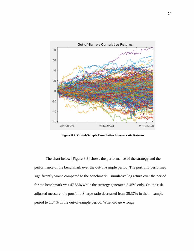
24

Figure 8.2: Out-of-Sample Cumulative Idiosyncratic Returns

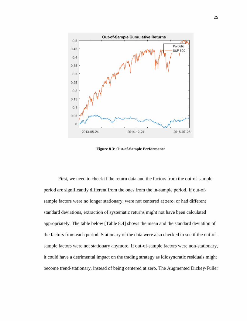
The chart below [Figure 8.3] shows the performance of the strategy and the

performance of the benchmark over the out-of-sample period. The portfolio performed

significantly worse compared to the benchmark. Cumulative log return over the period

for the benchmark was 47.56% while the strategy generated 3.45% only. On the risk-

adjusted measure, the portfolio Sharpe ratio decreased from 35.37% in the in-sample

period to 1.84% in the out-of-sample period. What did go wrong?

25

Figure 8.3: Out-of-Sample Performance

First, we need to check if the return data and the factors from the out-of-sample

period are significantly different from the ones from the in-sample period. If out-of-

sample factors were no longer stationary, were not centered at zero, or had different

standard deviations, extraction of systematic returns might not have been calculated

appropriately. The table below [Table 8.4] shows the mean and the standard deviation of

the factors from each period. Stationary of the data were also checked to see if the out-of-

sample factors were not stationary anymore. If out-of-sample factors were non-stationary,

it could have a detrimental impact on the trading strategy as idiosyncratic residuals might

become trend-stationary, instead of being centered at zero. The Augmented Dickey-Fuller

26

test was conducted to test for the null hypothesis of a presence of a unit root to test for

stationarity.

Table 8.4: Out-of-Sample Factor

The null hypothesis of a presence of a unit root was rejected for all 12 factors in

both periods, suggesting that stationary is maintained in the out-of-sample period. Out-of-

sample factors exhibit means that are slightly different from 0 and standard deviations

that are generally smaller than the standard deviations from the in-sample period. This

can suggest that either the estimated factor loadings were not robust or the short-term

market condition for the out-of-sample might be different from the long-term market

condition of the estimation period. To test that, a further analysis on the first factor,

Factor

Number

In-

Sample

Out-of-

Sample

In-

Sample

Out-of-

Sample

In-

Sample

Out-of-

Sample

In-

Sample

Out-of-

Sample

1 0.0000 0.1535 13.5146 8.1029 TRUE TRUE 0.001 0.001

2 0.0000 -0.0907 3.8392 2.3240 TRUE TRUE 0.001 0.001

3 0.0000 -0.2034 3.2998 3.1833 TRUE TRUE 0.001 0.001

4 0.0000 0.0076 2.9769 2.0501 TRUE TRUE 0.001 0.001

5 0.0000 0.1351 2.2948 2.0975 TRUE TRUE 0.001 0.001

6 0.0000 0.0783 2.0529 1.3555 TRUE TRUE 0.001 0.001

7 0.0000 -0.1206 1.9483 1.5516 TRUE TRUE 0.001 0.001

8 0.0000 -0.0330 1.7899 1.1707 TRUE TRUE 0.001 0.001

9 0.0000 0.0133 1.7629 1.5203 TRUE TRUE 0.001 0.001

10 0.0000 -0.0688 1.5699 1.0748 TRUE TRUE 0.001 0.001

11 0.0000 -0.0906 1.5087 1.0498 TRUE TRUE 0.001 0.001

12 0.0000 0.0254 1.4284 0.9899 TRUE TRUE 0.001 0.001

Mean Standard Deviation Stationary P value

27

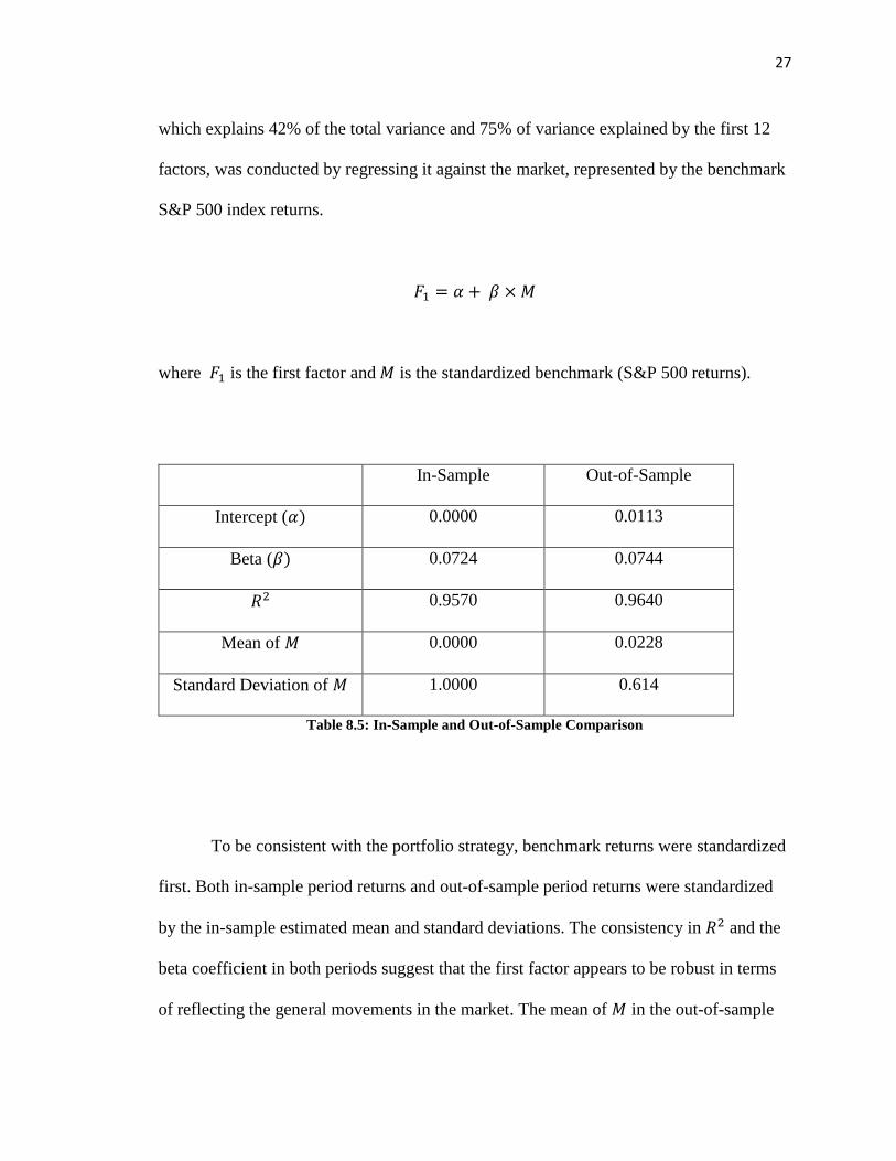
which explains 42% of the total variance and 75% of variance explained by the first 12

factors, was conducted by regressing it against the market, represented by the benchmark

S&P 500 index returns.

𝐹𝐹1 = 𝛼𝛼 + 𝛽𝛽 × 𝑀𝑀

where 𝐹𝐹1 is the first factor and 𝑀𝑀 is the standardized benchmark (S&P 500 returns).

In-Sample Out-of-Sample

Intercept (𝛼𝛼) 0.0000 0.0113

Beta (𝛽𝛽) 0.0724 0.0744

𝑅𝑅2 0.9570 0.9640

Mean of 𝑀𝑀 0.0000 0.0228

Standard Deviation of 𝑀𝑀 1.0000 0.614

Table 8.5: In-Sample and Out-of-Sample Comparison

To be consistent with the portfolio strategy, benchmark returns were standardized

first. Both in-sample period returns and out-of-sample period returns were standardized

by the in-sample estimated mean and standard deviations. The consistency in 𝑅𝑅2 and the

beta coefficient in both periods suggest that the first factor appears to be robust in terms

of reflecting the general movements in the market. The mean of 𝑀𝑀 in the out-of-sample

28

period is higher than the mean from the in-sample period. The standard deviation of 𝑀𝑀 in

the out-of-sample period is lower than the standard deviation from the in-sample period.

These suggest that the general market movements in the out-of-sample period have been

characterized by higher average returns with lower volatility compared to the estimation

period. This can be analyzed further by comparing the performance of the long portion of

the portfolio, which benefits when the selected securities increase in prices, and the short

portion of the portfolio, which benefits when the selected securities decrease in prices.

Correlations Comparison Portfolio

Portfolio

(Short

Portion)

Portfolio

(Long

Portion)

S&P 500

Portfolio 1.00

Portfolio (Short Portion) 0.33 1.00

Portfolio (Long Portion) 0.10 (0.91) 1.00 0.93

S&P 500 (0.17) (0.95) 0.93 1.00

Table 8.6: Out-of-Sample Correlation

Sensitivity Comparison Beta

Coefficient 𝑅𝑅2

Standard

Deviation

Sharpe

Ratio

Portfolio (0.72) 0.03 0.19% 1.84%

Portfolio (Short Portion) (1.69) 0.91 0.46% -4.32%

29

Portfolio (Long Portion) 1.73 0.86 0.44% 5.37%

S&P 500 1.00 1.00 0.82% 6.03%

Table 8.7: Out-of-Sample Performance Analysis

The correlation between the long portion of the portfolio and S&P 500 is .93 and

the correlation of the short portion of the portfolio and S&P 500 is -.95. This shows that

the relationship between our long and short positions to the market movement has not

changed compared to the estimation period. However, the correlation between the

portfolio strategy and S&P 500 is -.17, which is lower than the estimation period

correlation of -.04 between them. This change in correlation is likely to be the result of

the underperformance of the portfolio, rather than the portfolio becoming more

negatively correlated with the market in the forecasting period as the sensitivities of our

short and long components to the market, measured by beta, and correlation structure

have not changed. Our portfolio appears to remain uncorrelated to the market as desired.

The low 𝑅𝑅2 value of .03 from the regressing the out-of-sample portfolio results with S&P

500 reinforces this conclusion. Analysis can be further decomposed into long side of the

positions and short side of the positions to locate where the losses might be coming from.

During the out-of-sample period, the total cumulative log return from the long

positions was 22.69% with a Sharpe ratio of 5.37%. The total cumulative log return from

the short positions was -19.24% with a Sharpe ratio of -4.32%. These two components

add up to the total cumulative return of 3.45% for the portfolio. Clearly, most

underperformance came from the short positions. This illustrates a typical case of a

mean-reversion failure due to a prolonged directional movement in the market. As the

30

market moved upward for an unusually long period, the sell strategy greatly suffered. In

the next section, we will first discuss how to ensure that our strategy maintain

profitability even in directional markets without sacrificing returns excessively. Then we

will also discuss if any other enhancements can be made to further improve out-of-

sample performance.

31

IX. Failure Detection and Strategy Improvement Techniques

There are some previous studies on how to improve statistical arbitrage strategies

or detect potential big losses. Some try seek the optimal threshold to enter and exit with

respect to transaction cost to enter and exit. Leung and Li (2015) derive the optimal entry

and exit prices with respect to transaction cost by maximizing the expected difference

between the maximum expected profit and the distance between the current price and the

transaction cost. Leung and Li (2015) extends the model by incorporating a stop-loss

constraint to ensure that each position does not lose more than a certain amount. This

paper approaches the problem from a slightly different perspective. Rather than finding

an optimal threshold with respect to a given transaction cost, this paper aims to focus on

improving and testing the fundamental forecasting ability of the strategy.

Yeo and Papanicolaou (2016) points out that how few literature covers the risk of

relying on the mean reverting assumptions of the idiosyncratic returns in statistical

arbitrage literatures. Yeo and Papanicolaou (2016) suggest to control the risk of the

statistical arbitrage strategies by selecting securities that show high mean-reversion

speeds and selecting securities that showed a high goodness-of-fit. By testing the strategy

with the daily returns of 378 stocks in S&P 500 constituents from 2000 through 2014,

Yeo and Papanicolaou (2016) showed that the suggested strategy provided higher Sharpe

ratio. Mean-reversion speeds were estimated by fitting the mean-reverting cumulative

residuals into an Ornstein-Uhlenbeck process. Goodness-of-fit was measured by

comparing 𝑅𝑅2 values of the Ornstein-Uhlenbeck process. Based on out-of-sample test

results, Yeo and Papanicolaou (2016) suggest that both mean-reversion speed control and

𝑅𝑅2 control boosted the performance.

32

To improve the out-of-sample performance of the statistical arbitrage strategy

implemented in this study, we can start by searching for any patterns in successful

positions and unsuccessful positions. Furthermore, instead of looking at the aggregate

performance, each security performance is analyzed. The aggregate performance can be

decomposed into the following way, where 𝐵𝐵𝑖𝑖,𝑡𝑡 indicates return generated by ith security

in time t by taking a long position in the ith security. S indicates returns generated by

taking short positions.

𝑃𝑃𝑢𝑢𝑟𝑟𝑓𝑓 = ��𝐵𝐵𝑖𝑖,𝑡𝑡 + ��𝑆𝑆𝑖𝑖,𝑡𝑡

𝑇𝑇

𝑡𝑡=1

𝑛𝑛

𝑖𝑖=1

𝑇𝑇

𝑡𝑡=1

𝑛𝑛

𝑖𝑖=1

The out-of-sample portfolio returns can be sorted by their performance in the

following way. The below chart [Figure 9.1] illustrates aggregate cumulative

performance over the out-of-sample period per security.

33

Figure 9.1: Out-of-Sample Returns Per Securities

First, we can check if assets that fitted better in the estimation period tend to

perform better in the out-of-sample period. Two different goodness-of-fit can be

compared. First, 𝑅𝑅2 from the systematic exposure measuring step can be compared.

Higher 𝑅𝑅2 means that a larger part of returns was explained by systematic factors. The

out of sample performances were regressed in the following way. 𝑍𝑍 indicates a 430 by 1

vector in which each element indicates the cumulative out-of-sample performance for

each security. 𝑍𝑍𝑙𝑙 indicates cumulative returns generated by the long positions and 𝑍𝑍𝑠𝑠

indicates cumulative returns generated by the short positions. R indicates a 430 by 1

vector that includes individual 𝑅𝑅2 from the estimation of the systematic exposures. The

figure [Figure 9.2] below illustrates a scatterplot of returns and 𝑅𝑅2. Each regression

0 50 100 150 200 250 300 350 400 450

-2

-1

0

1

Cum

ulat

ive

Log

Ret

urns

Sorted Short Position Returns

0 50 100 150 200 250 300 350 400 450

-2

-1

0

1

2

Cum

ulat

ive

Log

Ret

urns

Sorted Long Position Returns

34

yielded 𝑅𝑅2 values of .006 and .048, suggesting that securities that were fitted well with

systematic factors did not necessarily performed better out-of-sample.

𝑍𝑍𝑙𝑙 = 𝛼𝛼𝑙𝑙 + 𝛽𝛽𝑙𝑙 × R + 𝜀𝜀𝑙𝑙

𝑍𝑍𝑠𝑠 = 𝛼𝛼𝑠𝑠 + 𝛽𝛽𝑠𝑠× R + 𝜀𝜀𝑠𝑠

Figure 9.2: Out-of-Sample Returns Versus Goodness of Fit

Next, 𝑅𝑅2 and mean reversion speed from fitting OU process in the cumulative

idiosyncratic process can be compared as Yeo and Papanicolaou (2016) suggested.

Ornstein-Uhlenbeck process is a stochastic process that is similar to an auto-regressive

process in the discrete time series realm. It illustrates a time series that follow Brownian

35

motion but shows a mean reverting tendency in the long run (Masindi, 2014). By fitting

the cumulative idiosyncratic returns into Ornstein-Uhlenbeck process, we can measure

standard deviations and mean reverting speeds. Yeo and Papanicolaou (2016) suggested

that cumulative idiosyncratic returns with faster mean-reversion speeds and higher

goodness-of-fit are likely to generate superior performances. Faster mean-reversion

speeds suggest that mean reversion will take place quickly and higher goodness-of-fit

suggests that the time series is more likely to follow the Ornstein-Uhlenbeck process

instead of the geometric Brownian motion with a unit root. The Ornstein-Uhlenbeck

process can be expressed in the following way where Ci is the cumulative idiosyncratic

returns for the ith asset, 𝑚𝑚𝑖𝑖 is the mean reversion level for the ith asset, 𝜅𝜅𝑖𝑖 is the mean

reversion parameter for the ith asset, and σ𝑖𝑖 is the standard deviation for the ith asset, and

W𝑖𝑖 is the Brownian motion (Wiener) process.

𝑎𝑎Ci(t) = 𝜅𝜅𝑖𝑖 �𝑚𝑚𝑖𝑖 − Ci(t)�𝑎𝑎t + σ𝑖𝑖𝑎𝑎W𝑖𝑖(t), 𝜅𝜅𝑖𝑖 > 0

The parameters for the Ornstein-Uhlenbeck process can be estimated as a discrete

autoregressive process with lag one. Estimated mean reversion speeds and goodness-of-

fit were regressed with the out of sample performance in the same way as the equation

above. The below table [Table 8.10] shows the result. Mean reversion speed was

measured as 1𝜅𝜅𝑖𝑖

. As low 𝑅𝑅2 for four different regressions illustrate, mean reversion speed

and goodness-of-fit of Ornstein-Uhlenbeck process do not seem to be correlated with out-

of-sample performance, unlike as Yeo and Papanicolaou (2016) suggested.

36

𝑍𝑍𝑙𝑙 = 𝛼𝛼𝑙𝑙 + 𝛽𝛽𝑙𝑙 × R + 𝜀𝜀𝑙𝑙

𝑍𝑍𝑠𝑠 = 𝛼𝛼𝑠𝑠 + 𝛽𝛽𝑠𝑠× R + 𝜀𝜀𝑠𝑠

𝑅𝑅2 of the Regression Result

Short Positions

Returns

Long Positions

Returns

R = Goodness of Fit of OU Process 0.0016 0.0148

R = Mean Reversion Speed 0.0010 0.0186

Table 9.3: OU Process and Out-of-Sample Returns

There might be several reasons why screening method by Yeo and Papanicolaou

(2016) did not seem consistent in this dataset. First, estimation window and the selected

individual stocks are different. Second, instead of screening with parameters based on the

entire sample period, Yeo and Papanicolaou (2016) estimated the parameters with

different estimation windows and made stock selections at each time step. Yeo and

Papanicolaou (2016) explain that the mean-reversion speed is normalized by the

estimation window since the estimated mean-reversion parameter usually depends on the

length of the estimation window.

The strategy tends to perform worse out-of-sample when cumulative idiosyncratic

returns do not oscillate as they did in-sample and no longer show mean-reverting nature.

Checking for stationarity can inform us whether the time series is likely to be stationary

37

or not. Augmented Dickey-Fuller test was conducted to test for this. The Augmented

Dickey-Fuller test on the cumulative idiosyncratic returns in-sample yielded the

following results. Out of 430 securities, the null hypothesis of a unit root was rejected in

195 securities, suggesting that these time series are stationary. The rest 235 securities

failed to reject the null hypothesis of a unit root. The average achieved returns per

securities that were stationary were compared with the average achieved returns per

securities that were not stationary. The cumulative returns per security were divided by

the number of time periods to compare in-sample and out-of-sample performance fairly.

As shown below, returns generated by the securities that were stationary outperformed.

This is not surprising as the strategy relies on buy-low and sell-high concept.

Stationary Not

Stationary

In-Sample

Number of Securities 195 235

Average Returns Per

Security Per Time-Period

Short Positions 0.01429% 0.00347%

Long Positions 0.02894% 0.01789%

Out-Of-

Sample

Number of Securities 24 406

Average Returns Per

Security Per Time-Period

Short Positions -0.00017% -0.00704%

Long Positions 0.00600% 0.00769%

Table 9.4: Out-of-Sample Returns and Stationarity

38

However, out-of-sample analysis yielded an interesting result. Only 24 out of 430

cumulative idiosyncratic returns of the securities were considered as stationary.

Furthermore, returns underperformed compared to in-sample returns across both

stationary and non-stationary time series. Whether taking positions only when the time

series is believed to be stationary can add value was further tested by testing a modified

version of the strategy. The strategy is performed as followed. At each time step,

stationary test for the individual cumulative idiosyncratic returns is conducted. If it is

considered as stationary, the same one standard deviation trading rule is followed. If the

time series is not considered as stationary, no trading decision takes place. Out of 966

time-periods in the out-of-sample period, this strategy was implemented starting with 16th

time-period to ensure that there are enough observations to conduct the ADF test.

𝑆𝑆𝑖𝑖𝑡𝑡 = 0 𝑎𝑎𝑛𝑛𝑎𝑎 𝐵𝐵𝑖𝑖𝑡𝑡 = 0 𝑢𝑢𝑛𝑛𝑙𝑙𝑢𝑢𝑢𝑢𝑢𝑢

𝑆𝑆𝑖𝑖𝑡𝑡 = −1 𝑖𝑖𝑓𝑓 𝑐𝑐𝑖𝑖𝑡𝑡 > 𝑍𝑍𝑖𝑖 and 𝒙𝒙𝑖𝑖,1:𝑡𝑡 𝑖𝑖𝑢𝑢 𝑢𝑢𝑡𝑡𝑎𝑎𝑡𝑡𝑖𝑖𝑠𝑠𝑛𝑛𝑎𝑎𝑟𝑟𝑠𝑠

𝐵𝐵𝑖𝑖𝑡𝑡 = 1 𝑖𝑖𝑓𝑓 𝑐𝑐𝑖𝑖𝑡𝑡 < −𝑍𝑍𝑖𝑖 and 𝒙𝒙𝑖𝑖,1:𝑡𝑡 𝑖𝑖𝑢𝑢 𝑢𝑢𝑡𝑡𝑎𝑎𝑡𝑡𝑖𝑖𝑠𝑠𝑛𝑛𝑎𝑎𝑟𝑟𝑠𝑠

𝑃𝑃𝑡𝑡 = 12∑ |𝑆𝑆𝑖𝑖,𝑡𝑡−1|𝑛𝑛

𝑖𝑖=1∑ 𝑆𝑆𝑖𝑖,𝑡𝑡−1𝑛𝑛𝑖𝑖=1 × 𝒙𝒙𝑖𝑖𝑡𝑡 + 1

2∑ |𝐵𝐵𝑖𝑖,𝑡𝑡−1|𝑛𝑛𝑖𝑖=1

∑ 𝐵𝐵𝑖𝑖,𝑡𝑡−1𝑛𝑛𝑖𝑖=1 × 𝑥𝑥𝑖𝑖𝑡𝑡

The performance result suggests that this is not likely to be a superior strategy.

The average returns per security per time-period for the short positions was -.1700% and

0.0797% for the long positions. Although the long positions returns were better, the short

positions returns were significantly worse, which caused the total cumulative return of

the strategy to wind up at -94.18%. Although the stationarity is necessary for the strategy

to perform well, the actual implementation of it is not easy without looking-back bias. If

39

the times series to be invested can be selected by the stationarity of the full-length time

series, it can enhance the performance, as shown in the above table. However, at each

time step, without looking forward in the future, the best information about the

stationarity of the time series can be only estimated by the time series up to that point,

which might not reflect if the time series will stay stationary throughout the trading

period.

Markov regime switching model was tested to improve the strategy as well. Many

pairs trading strategies often assume that spreads between two cointegrated stocks can

oscillate around a mean of the spread. However, fundamental change in the company or

the market structure might cause the spread to no longer revert to the historical mean or

revert to a different equilibrium level. Bock and Mestel (2008) applied Markov regime

switching model with switching mean and variance to improve pairs trading strategy.

Markov chains were originally developed as a part of extension of the law of large

numbers to dependent events (Merrill, 2010). Markov chain introduce the concept that,

instead of a sequence of random observations generated by one state, there might be

multiple states that generates random variables and the determination of current states

might depend on what the previous states were.

In finance, hidden Markov Models are more often used as most of states are

unobservable. We can assume that the current observations are generated by an

unobservable state 𝑆𝑆𝑡𝑡. 𝑆𝑆𝑡𝑡 emits observations based on its distribution. At each time step,

based on transition probabilities, the state might change and the probability distribution

will also change accordingly. Often, the transition from one state to another state is

simplified and assumed to be dependent on only the previous state. Instead of assuming

40

that the transition of states are deterministic, HHM assumes that there must have been

predictable stochastic process that causes states to shift from one to another (Hamilton,

2005). Although we cannot directly observe states, we can estimate the states based on

observed emissions. Consider the following process where 𝐾𝐾𝑡𝑡 = 1,2 and 𝜀𝜀𝑡𝑡 follows a

normal distribution with zero mean and variance given by 𝜎𝜎K2.

𝑋𝑋𝑡𝑡 = 𝜇𝜇𝐾𝐾𝑡𝑡 + 𝜀𝜀𝑡𝑡

𝜀𝜀𝑡𝑡 ~ 𝑁𝑁(0,𝜎𝜎𝐾𝐾𝑡𝑡2 )

This is a simple case of how normally distributed variable can behave across

different latent regimes (Perlin, 2015). This process can be estimated by Bayesian

inference or maximum likelihood. In this study, maximum likelihood estimation method

of Perlin (2015) was implemented. The log likelihood function can be estimated as

follows.

ln 𝐿𝐿 = � ln�(𝑓𝑓(2

𝑗𝑗=1

𝑇𝑇

𝑡𝑡=1

𝑋𝑋𝑡𝑡 | 𝐾𝐾𝑡𝑡 = 𝑗𝑗,𝛩𝛩)Pr ( 𝐾𝐾𝑡𝑡 = 𝑗𝑗))

𝛩𝛩 indicates the set of parameters. Likelihood function in each state are weighted

averaged by the probabilities of each states. Although it is possible to estimate the model

with many regimes, estimating parameters accurately becomes difficult as the number of

regimes increase. Therefore, most HHM applications assume two or three different

regimes (Hamilton, 2010). In this study, HHM is implemented to check if it can improve

41

the trading strategy. States and parameters were estimated for each idiosyncratic return.

Then, the adjusted trading rule was applied to check if knowing the current state of the

idiosyncratic returns can improve the performance. The states and trading rules are as

follows.

𝑋𝑋𝑖𝑖,𝑡𝑡 = 𝜇𝜇𝐾𝐾𝑖𝑖,𝑡𝑡 + 𝜀𝜀𝑖𝑖,𝑡𝑡

𝜀𝜀𝑖𝑖,𝑡𝑡 ~ 𝑁𝑁(0,𝜎𝜎𝐾𝐾𝑖𝑖,𝑡𝑡2 )

𝑆𝑆𝑖𝑖𝑡𝑡 = 0 𝑎𝑎𝑛𝑛𝑎𝑎 𝐵𝐵𝑖𝑖𝑡𝑡 = 0 𝑢𝑢𝑛𝑛𝑙𝑙𝑢𝑢𝑢𝑢𝑢𝑢

𝑆𝑆𝑖𝑖𝑡𝑡 = −1 𝑖𝑖𝑓𝑓 𝑐𝑐𝑖𝑖𝑡𝑡 > 𝑍𝑍𝑖𝑖 and 𝜇𝜇𝐾𝐾𝑖𝑖,𝑡𝑡 < 0

𝐵𝐵𝑖𝑖𝑡𝑡 = 1 𝑖𝑖𝑓𝑓 𝑐𝑐𝑖𝑖𝑡𝑡 < −𝑍𝑍𝑖𝑖 and 𝜇𝜇𝐾𝐾𝑖𝑖,𝑡𝑡 > 0

𝑃𝑃𝑡𝑡 = 12∑ |𝑆𝑆𝑖𝑖,𝑡𝑡−1|𝑛𝑛

𝑖𝑖=1∑ 𝑆𝑆𝑖𝑖,𝑡𝑡−1𝑛𝑛𝑖𝑖=1 × 𝒙𝒙𝑖𝑖𝑡𝑡 + 1

2∑ |𝐵𝐵𝑖𝑖,𝑡𝑡−1|𝑛𝑛𝑖𝑖=1

∑ 𝐵𝐵𝑖𝑖,𝑡𝑡−1𝑛𝑛𝑖𝑖=1 × 𝑥𝑥𝑖𝑖𝑡𝑡

where 𝑋𝑋 indicates idiosyncratic return, 𝜇𝜇𝐾𝐾𝑖𝑖,𝑡𝑡 indicates expected idiosyncratic return for ith

asset at time t in state K.

This is based on assumption that there might be two different states that

idiosyncratic returns are generated from and we can benefit from factoring that into the

trading strategy. The strategy goes as follows. In the original strategy, if cumulative

residual of ith asset at time t reaches the level that is higher than the Z score, the sell

signal was generated. In this Markov enhanced version, sell signal is only generated if the

expected value of the idiosyncratic returns is less than zero. The rationale behind this is

that, even if the cumulative idiosyncratic returns might be higher than the threshold and

we expect it to come down, the idiosyncratic returns might be in the state where

42

cumulative idiosyncratic returns are expected to continue to rise. This can be viewed

consistent with the “momentum” trading strategies. The same logic applies to buy

signals.

The signal generation procedure was conducted in the following way. 430 Each

stock’s in-sample period idiosyncratic returns and out-of-sample period idiosyncratic

returns were combined and the hidden Markov model was fitted. After gathering filtered

state probabilities and expected idiosyncratic return parameters, the trading signals were

generated at each time step. The performance of the new strategy is shown below.

Figure 9.5: Enhanced Out-of-Sample Returns

43

The enhanced strategy returned 19.49% cumulative returns among the period

compared to the benchmark performance of 47.56%. The Sharpe ratio was 6.07%

compared to the Sharpe ratio of 6.03% for the benchmark. The correlation between two

returns was -.03. Low correlation and the satisfactory Sharpe ratio suggest that this

strategy can add value. Although the absolute performance is low, if the stream of returns

is not correlated to the market and has a high Sharpe ratio, the leverage can be often used

to enhance the magnitude of the performance. Both long position returns and short

position returns appeared acceptable as shown below.

Correlations Comparison Portfolio

Portfolio

(Short

Portion)

Portfolio

(Long

Portion)

S&P 500

Portfolio 1.00

Portfolio (Short Portion) 0.18 1.00

Portfolio (Long Portion) 0.46 (0.79) 1.00

S&P 500 (0.03) (0.93) 0.82 1.00

Table 9.6: Enhanced Out-of-Sample Returns Correlations

Sensitivity Comparison Beta

Coefficient 𝑅𝑅2

Standard

Deviation

Sharpe

Ratio

44

Portfolio (0.08) 0.00 0.33% 6.07%

Portfolio (Short Portion) (1.57) 0.87 0.49% -2.05%

Portfolio (Long Portion) 1.25 0.68 0.54% 5.60%

S&P 500 1 1 0.82% 6.03%

Table 9.7: Enhanced Out-of-Sample Returns Statistics

A few things need to be noted. First, short position returns have improved but it

still yields negative returns. However, as the goal of the strategy is to provide a positive

return net of short and long positions, this is not as big of a concern. Second, both betas

of short and long position returns are over 1 in absolute values, suggesting that the each

components of the strategy might be riskier than the benchmark. Third, most importantly,

this might suffer from a forward looking bias. The filtered probability of the states and

the expected value parameter 𝜇𝜇𝐾𝐾𝑖𝑖,𝑡𝑡 for the Hidden Markov Models for each stock were

estimated with the idiosyncratic returns from both in-sample and out-of-sample periods.

To truly test this strategy in out-of-sample period, the estimation of filtered probability

and the expected values has to take place at each time step for each stocks. However, this

was computationally too expensive for the scope of this study. Each estimation took

roughly 30 seconds, which took a total of 215 minutes (30*430/60) for 430 securities. To

repeat this at each 966 time periods in the out-of-sample period would have taken 3461

hours without any parallel computing.

45

X. Conclusion

The purpose of this thesis was to evaluate a statistical arbitrage strategy and

suggest enhancements to improve out-of-sample performance by extending the

generalized pairs trading model by Avellaneda and Lee (2010). By removing systematic

returns from stock returns, we extracted idiosyncratic returns. Based on previous

empirical findings and theoretical support (Arbitrage Pricing Theory), we constructed a

trading strategy that assumes the mean reversion of cumulative idiosyncratic returns of

stocks.

Implementation of the strategy to U.S. equities from 2004 January through 2012

December yielded a daily Sharpe ratio, calculated by dividing daily returns by daily

standard deviation, of 35.37% versus 1.42% of the benchmark S&P 500. As desired,

implementation of long and short positions resulted in an uncorrelated strategy, as shown

by the correlation of -.04 during the period.

However, the out-of-sample performance result did not appear impressive. From

January 2013 through October 2016, the portfolio Sharpe ratio decreased from 35.37% in

the in-sample period to 1.84% in the out-of-sample period while the Sharpe ratio of S&P

was 6.03%. Stationarity of factors, stationarity of cumulative idiosyncratic returns,

goodness of estimations, mean reverting speeds of Ornstein-Uhlenbeck process, and

Hidden Markov regimes were analyzed to enhance the original strategy. Hidden Markov

regime switching model was the only enhancement that improved the result. The

enhanced strategy generated the Sharpe ratio of 6.07% while still uncorrelated to the

market. However, it should be noted that it might have suffered from a forward looking

bias.

46

There are several areas of this study that can be further improved. For example, it

will be valuable to test if any specific sectors yield better results. Some sectors are known

to be more cyclical and some are known to be less cyclical. Factors can be further studies

as well. Unlike interest rates factor models, equity PCA factors are more difficult to tie

with economic theories. The first factor is likely to represent the general market

movement. It might be valuable to test if any pattern can be found between factors and

stocks. For example, one can test if stocks with high leverage have positive correlation

with any of the factors. Lastly, testing different estimation windows can yield interesting

insights on the ideal length of data to capture both long enough and relevant enough data.

47

BIBLIOGRAPHY Avellaneda, Marco, and Jeong-Hyun Lee. "Statistical arbitrage in the US equities

market." Quantitative Finance 10.7 (2010): 761-782. Azeez, A. A., and Yasuhiro Yonezawa. "Macroeconomic factors and the empirical

content of the Arbitrage Pricing Theory in the Japanese stock market." Japan and the world economy 18.4 (2006): 568-591.

Bai, Jushan, and Serena Ng. "Determining the number of factors in approximate factor

models." Econometrica 70.1 (2002): 191-221. Benaković, Dubravka, and Petra Posedel. "Do macroeconomic factors matter for stock

returns? Evidence from estimating a multifactor model on the Croatian market." Business Systems Research 1.1-2 (2010): 39-46.

Bock, Michael, and Roland Mestel. "A regime-switching relative value arbitrage

rule." Operations Research Proceedings 2008. Springer Berlin Heidelberg, 2009. 9-14. Connor, Gregory, and Robert A. Korajczyk. "A test for the number of factors in an

approximate factor model." the Journal of Finance 48.4 (1993): 1263-1291. Engel, Charles. "Can the Markov switching model forecast exchange rates?." Journal of

International Economics 36.1-2 (1994): 151-165. Gatev, Evan, William N. Goetzmann, and K. Geert Rouwenhorst. "Pairs trading:

Performance of a relative-value arbitrage rule." Review of Financial Studies 19.3 (2006): 797-827.

Hamilton, James D. "Regime switching models." Macroeconometrics and Time Series

Analysis. Palgrave Macmillan UK, 2010. 202-209. Hong, Gwangheon, and Raul Susmel. "Pairs-trading in the Asian ADR

market." University of Houston, Unpublished Manuscript (2003).

48

Josse, Julie, Jérôme Pagès, and François Husson. "Multiple imputation in principal

component analysis." Advances in data analysis and classification 5.3 (2011): 231-246.

Khandani, A., and A. Lo. "What happened to the quants in august 2007?(digest

summary)." Journal of investment management 5.4 (2007): 29-78. Krauss, Christopher, and Johannes Stübinger. Nonlinear dependence modeling with

bivariate copulas: Statistical arbitrage pairs trading on the S&P 100. No. 15/2015. IWQW Discussion Paper Series, 2015.

Leung, Tim, and Xin Li. "Optimal mean reversion trading with transaction costs and

stop-loss exit." International Journal of Theoretical and Applied Finance 18.03 (2015): 1550020.

Liew, Jim, and Ryan Roberts. "US equity mean-reversion examined." Risks 1.3 (2013): 162-175.

Lo, Andrew W., and A. Craig MacKinlay. "When are contrarian profits due to stock market overreaction?." Review of Financial studies 3.2 (1990): 175-205.

Masindi, Khuthadzo. Statistical arbitrage in South African equity markets. Diss.

University of Cape Town, 2014. Merrill, S. "Markov chains for identifying nonlinear dynamics." Nonlinear dynamical

systems analysis for the behavioral sciences using real data (2010): 401-423. Papanicolaou, George, and Joongyeub Yeo. "Risk Control of Mean-Reversion Time in

Statistical Arbitrage." (2016). Perlin, Marcelo. "MS_Regress-the MATLAB package for Markov regime switching models." (2015). Roll, Richard, and Stephen A. Ross. "An empirical investigation of the arbitrage pricing

theory." The Journal of Finance 35.5 (1980): 1073-1103.