Finance and Economics Discussion Series Divisions of Research & Statistics and Monetary Affairs

Federal Reserve Board, Washington, D.C.

An Arbitrage-Free Three-Factor Term Structure Model and the Recent Behavior of Long-Term Yields and Distant-Horizon

Forward Rates

Don H. Kim and Jonathan H. Wright 2005-33

NOTE: Staff working papers in the Finance and Economics Discussion Series (FEDS) are preliminary materials circulated to stimulate discussion and critical comment. The analysis and conclusions set forth are those of the authors and do not indicate concurrence by other members of the research staff or the Board of Governors. References in publications to the Finance and Economics Discussion Series (other than acknowledgement) should be cleared with the author(s) to protect the tentative character of these papers.

An Arbitrage-Free Three-Factor Term Structure Model and the Recent Behavior of Long-

Term Yields and Distant-Horizon Forward Rates

Don H. Kim and Jonathan H. Wright*

Federal Reserve Board, Washington DC

August 2005

Abstract: This paper reviews a simple three-factor arbitrage-free term structure model

estimated by Federal Reserve Board staff and reports results obtained from fitting this

model to U.S. Treasury yields since 1990. The model ascribes a large portion of the

decline in long-term yields and distant-horizon forward rates since the middle of 2004 to

a fall in term premiums. A variant of the model that incorporates inflation data indicates

that about two-thirds of the decline in nominal term premiums owes to a fall in real term

premiums, but estimated compensation for inflation risk has diminished as well.

JEL Classification: E43

Keywords: Forward Rates, Term-Structure Model, Arbitrage-Free Pricing, Term

Premiums

* Division of Monetary Affairs, Federal Reserve Board, Washington DC 20551. We are grateful to Mary Zaki for excellent research assistance and to Jim Clouse and Brian Madigan for helpful comments. All remaining errors are our own. The views expressed in this paper are solely the responsibility of the authors and should not be interpreted as reflecting the views of the Board of Governors of the Federal Reserve System or of any other employee of the Federal Reserve System. Email addresses for the authors are don.h.kim@frb.gov and jonathan.h.wright@frb.gov.

1

1. Introduction.

The target federal funds rate of the Federal Open Market Committee (FOMC) increased

225 basis points from just before the June 2004 FOMC meeting to July 2005. This

tightening of monetary policy was greater than had been expected in June 2004, judging

from money market futures quotes. Nevertheless, longer-term yields dropped over this

time period, with the ten-year yield falling 50 basis points, while the ten year

instantaneous forward rate declined 150 basis points.

This drop in long-term forward rates during a tightening episode is quite unusual.

During the tightening episodes of 1994 and 1999, for example, forward rates moved up

appreciably, on net, as the stance of policy firmed.

The yield on a nominal Treasury security can be decomposed into the sum of the

compounded expected future short-term interest rate over the maturity of the bond and a

risk or term premium to compensate investors for the uncertain return on holding the

bond (over a horizon less than its maturity). The expected future short-term interest rate

and the term premium are, of course, not directly observable. This paper uses an

arbitrage-free three-factor term structure model of Kim and Orphanides (2004) that is

based on the work of Duffie and Kan (1996) and Duffee (2002) to estimate a

decomposition of the term structure of nominal interest rates into expected future short

rates and term premiums. The model attributes much of the decline in longer-term yields

over the last year to a fall in term premiums. This paper also uses a variant of the model

that incorporates inflation data (Kim (2004)) to further parse expected future short rates

and term premiums into real and inflation components.

2

This main focus of this paper is on describing the estimation of expected future

rates and term premiums, rather than on discussing the reasons why term premiums might

have fallen over the last year. However, we briefly review some of the possible

explanations that analysts have discussed. These explanations can essentially be reduced

to an assertion that the demand for longer-maturity obligations has increased relative to

supply, leading investors to demand smaller excess returns for holding these securities.

In turn, the increase in relative demand for longer-maturity fixed-income obligations

might be traced to the following factors:

1. Increased attractiveness of longer-maturity obligations owing to better anchored

inflation expectations and a reduction in the volatility of real activity. Several authors

have documented a decline in real volatility in the early 1980s (see e.g. McConnell and

Perez-Quiros (2000)). Some authors have also found a decline in inflation volatility at

about that time (see e.g. Ahmed, Levin, and Wilson (2002)). One question in the Survey

of Professional Forecasters asks respondents to assign probabilities to real GDP growth

and inflation being in each of ten bins the current and subsequent years. The averages of

these forecasts across respondents give simple density forecasts that can be used to

construct standard deviations for output growth and inflation1 which are direct measures

of agents' uncertainty, not merely the dispersion of their beliefs. Figure 1 shows the

standard deviation of the density forecasts for this year's and next year's output growth

1 For example, for output growth, the density forecast gives probabilities of real GDP growth in the current and subsequent years being greater than 6 percent, between 5 and 6 percent, between 4 and 5 percent, and so on, with the lowest bin being less than -2 percent. To construct the implied standard deviations, we assign the probability in each bin to the midpoint of that bin (e.g. the probability of growth being between 5 and 6 percent is assumed to be the probability of growth being 5.5 percent) and we assign the probabilities in the highest and lowest bins to +6.5 percent and -2.5 percent, respectively. We then simply compute the square root of the variance of this discretized density function.

3

and inflation from the Survey of Professional Forecasters each May since 1992. These

standard deviations have indeed declined over the last couple of years to historically low

levels, giving a very direct sense in which macroeconomic uncertainty has diminished.

Implied volatility on short-term interest rates implied by options has also trended down in

recent years.

2. Increased foreign interest in U.S. longer-term obligations as a result of intervention by

official institutions2 (Bernanke, Reinhart and Sack (2004)), less home bias of foreign

investors, and rapid economic growth rates in countries with high savings rates. Figure 2

shows the proportions of Treasury securities held by foreign official institutions in

custody accounts at the Federal Reserve Bank of New York and by all foreign investors.

Both have been trending up in recent years, though the proportion of Treasury securities

held by foreign official institutions has actually edged lower so far this year.

3. Increased demand for longer-maturity securities stemming from the prospect of

corporate pension fund reform in the United States, Europe, and elsewhere that might

encourage pension funds to be more fully funded and to take steps to better match the

duration of their assets and liabilities. U.S. defined-benefit pension plans held about $1¾

trillion in assets as of the first quarter of this year, but only about 30 percent of assets

were held in the form of Treasury, agency, and corporate securities.3 To date, there has

2 On July 21, 2005, ten-year Treasury yields jumped about 11 basis points, with foreign yields relatively little changed, immediately after the announcement of the renminbi revaluation by the People's Bank of China. This is consistent with a market perception that foreign official demand has been a factor driving down U.S. yields, though it could also owe at least in part to many other explanations, such as the potential for slightly higher import price inflation in the U.S. 3 Source: Supplementary Table L119b of the Flow of Funds Accounts.

4

been little evidence of a sizable portfolio shift at pension funds toward long-duration

bonds, and in any case equities are likely to be longer duration assets than any bonds.

Nonetheless, judging from anecdotal reports, bond investors might be attaching some

odds to scenarios in which pension funds tilt the composition of their portfolios toward

such assets substantially over time.

4. Apparently modest appetite for business capital spending, relative to the level of

corporate profits, in many countries in the industrialized and developing world.

5. Some analysts have pointed to demographics, as substantial cohorts of the populations

of industrialized economies near retirement. In this story, aging populations in many

industrialized countries are expected to increasingly shift their holdings away from risky

assets such as equities towards bonds and other assets that are perceived to be relatively

safe, and those anticipated portfolio shifts are thought by some to be placing downward

pressures on long-term yields at present. However, it can hardly be claimed that there

has been a substantial or unexpected shift in demographics since June 2004.

6. Low supply of longer-term fixed-income obligations, reflecting subdued corporate

bond issuance and the Treasury's decision in 2001 to discontinue auctions of the thirty-

year bond. However, in the May mid-quarter refunding statement, the Treasury

announced that it was considering reintroducing regular issuance of a thirty-year nominal

bond in February 2006.

5

Whatever the merits of any of these explanations, the term premium estimates that we

report in this paper should be thought of as "catch-all" measures that combine all of these

effects and indeed anything else that might affect the price of Treasury securities other

than expected future monetary policy.

The plan for the remainder of the paper is as follows. In section 2, we describe

the three-factor nominal arbitrage-free term structure model. Section 3 reports the

implied decomposition of Treasury yields and forward rates into expected future rates

and term premiums. Section 4 briefly describes the extension of this model to the real

term structure, by incorporating data on inflation. Finally, section 5 reports the implied

decomposition of nominal Treasury yields and forward rates into expected future real

rates, expected future inflation, real term premiums, and inflation risk premiums. Section

6 concludes and discusses some directions for future work.

2. Three-Factor Arbitrage-Free Term Structure Model

2.1 Pricing of real and nominal zero-coupon bonds.

Consider an n-period real zero-coupon bond that is being priced at time t and that pays

one unit of the consumption good at time t n+ . First consider a discrete-time model in

which the representative investor has a utility function of the form

0 ( )jj t ju cβ∞= +Σ (1)

where tc denotes consumption in period t and ( )tu c is the utility in that time period.

The first-order condition for maximization of (1) requires that the price of this n-period

real zero-coupon bond be

6

,'( )

( )'( )

R n t nn t t

t

u cP E

u cβ +=

where '(.)u denotes marginal utility in a given time period. Next consider a continuous-

time model in which the representative investor maximizes a utility function of the form

0( ( ( )))st sE e u c t s dsδ∞ −

=∫ + (2)

where ( )c t denotes instantaneous consumption at time t and (.)u denotes the

instantaneous utility function. The first-order condition for utility maximization of (2) is

entirely analogous, requiring that the price of the n-period real zero-coupon bond be

,'( ( ))( )

'( ( ))R n

n t tu c t nP E e

u c tδ− +

=

where '(.)u denotes instantaneous marginal utility. This can be written as

,( )( )

( )

RR

n t t R

m t nP Em t

+= (3)

where ( ) '( ( ))R tm t e u c tδ−= is the continuous-time stochastic discount factor, or pricing

kernel.4

This paper, however, focuses mainly on nominal rather than real bonds. A

nominal n-period zero-coupon bond pays $1 in nominal terms at time t n+ , or 1( )Q t n+

in real terms, where ( )Q t denotes the price index. The first-order condition for utility

maximization requires that the price of the n-period nominal zero-coupon bond be

4 Stochastic discount factors have different interpretations in discrete and continuous-time. The discrete-time stochastic discount factor is the marginal rate of substitution between consumption in two time periods. As can be seen from the definition here, the continuous-time stochastic discount factor refers instead to the level of marginal utility. See Cochrane (2001).

7

,'( ( )) ( )( )

'( ( )) ( )n

n t tu c t n Q tP E e

u c t Q t nδ− +

=+

which can be written as

,( )( )

( )n t tm t nP E

m t+

= (4)

where ( )( )( )

Rm tm tQ t

= is the continuous-time nominal stochastic discount factor.

2.2 The Model. The model of the nominal term structure described here is the implementation by Kim

and Orphanides (2004) of an arbitrage-free three-factor term structure model proposed by

Duffee (2002), building on work of Duffie and Kan (1996). The model of Kim and

Orphanides (2004) is model EA0(3) in the terminology of Duffee (2002), but it adopts a

different normalization of the factors and has the novel feature of being augmented by

survey data. The model assumes that the pricing relationship (4) holds for all bonds.

Hence, there are no arbitrage opportunities—once risk is taken into account—from

buying one security and selling short some combination of other securities. This is what

is meant by arbitrage-free pricing. The model furthermore assumes that the time-series

behavior of the yield curve can be described quite well by three underlying latent factors.

In principle, the factors could be proxies for the level, slope, and curvature of the yield

curve, or macroeconomic variables as used by authors such as Rudebusch and Wu

(2003). But the model discussed in this paper leaves the factors as latent variables.5

5 Specifying the factors as latent variables has the advantage of being more robust to model misspecification, but the disadvantage of making the factors harder to interpret.

8

Concretely, the model specifies that ( )x t is a three-dimensional vector of latent factors6

that follow the continuous-time analogue of a vector autoregression known as a

multivariate Ornstein-Uhlenbeck process, assuming that

( ) ( ) ( )dx t Kx t dt dB t= + Σ (5)

where K and Σ are 3x3 constant matrices and ( )B t is a three-dimensional standard

Brownian motion and that the instantaneous interest rate is an affine function of these

factors:

0( ) ' ( )r t x tρ ρ= + (6)

where 0ρ is a constant and ρ is a 3x1 vector. Assume further that

( ) ( ) ( ) ' ( )( )

dm t r t dt t dB tm t

λ= − − (7)

and

( ) ( )t x tλ φ= + Φ (8)

where φ is a 3x1 vector, Φ is a 3x3 matrix and ( )tλ is a 3x1 vector. The interpretation

of equation (7) is that the growth rate of ( )m t reflects the risk-free interest rate and an

adjustment for the sources of uncertainty in this model—the three Brownian motions in

( )B t , while the elements of ( )tλ give the market prices of each of these risks. And

equation (8) specifies that ( )tλ is an affine function of the factors ( )x t .7 Substituting

equations (5), (6), (7) and (8) into equation (4) yields

, exp( ( ) ( ) ' ( ))n tP a n b n x t= +

6 This theoretical model could of course easily be adapted to have any number of latent factors. 7 The model as it stands is not identified--rotations of the factors would imply the same yields with different parameters. Identification can be achieved by imposing the normalization that K is a lower triangular matrix and Σ is a diagonal matrix.

9

where the functions ( )a n and ( )b n are given as the solutions to a set of ordinary

differential equations (Duffie and Kan (1996), Duffee (2002)). Closed-form expressions

for these functions can be found in Langetieg (1980) and Kim and Orphanides (2004).

Hence the yield on an n-year nominal zero-coupon bond, ,n ty , will be affine in the

factors:

, ,1 1log ( ( ) ( ) ' ( ))n t n ty P a n b n x tn n

= − = − +

and the n-year instantaneous forward rate, ,n tf will be

,,

log ( ) ( ) ' ( )n tn t

P da n db nf x tn dn dn

∂= − = − −

∂

The model can be written in state space form in which weekly observations of

zero-coupon bond yields8 are the observed data and the factors ( )x t are the unobservable

state variables. The measurement equation is

't t to a B x η= + +

where to is an qx1 vector of zero-coupon yields of maturities 1n , 2n ... qn ,

1 2( , ,... ) '

qn n na a a a= , B is a 3xq matrix, the ith column of which is inb and tη is a vector of

measurement errors, assumed to be Gaussian. The transition equation is

( ) ( 1)Ktx t e x t ε= − +

where 1 '0~ (0, ' )Ks K s

t N e e dsε ∫ ΣΣ which is the discretization of (5), with the units of time

measured in weeks.9 This model may be estimated by the Kalman filter, and filtered and

8 The data used are weekly (Wednesday) zero-coupon term structure data, with maturities of 3 months, 6 months, 1 year, 2 years, 4 years, 7 years and 10 years. The zero-coupon yields for maturities of at least one year used in the estimation are taken from the Svensson curve that is fitted to off-the-run Treasury coupon securities at the Federal Reserve Board. Treasury bill yields are used for 3 month and 6 month interest rates.

10

smoothed estimates of the state vector ( )x t may be deduced. Filtered estimates give the

expectation of ( )x t conditional on the information set at time t; smoothed estimates give

the expectation of ( )x t conditional on all the observed data.

It is straightforward to include survey data within this Kalman filter framework.

The model uses monthly data on the six-month and twelve-month-ahead forecasts of the

three-month T-Bill yield from Blue Chip Financial Forecasts and semiannual data on the

average expected three-month T-Bill yield from six to eleven years hence, also from Blue

Chip. In weeks where these surveys are observed, they are incorporated in the

measurement equation and treated as noisy estimates of the underlying latent expected

three-month interest rate (the expected three-month interest rate plus Gaussian

measurement error). The dimension of the observable vector thus varies between m and

m+3. For more details of the incorporation of survey data into the estimation, see Kim

and Orphanides (2004).

The sample period for the estimation results reported in this paper is from July

1990 to July 2005. With this relatively short sample, the survey is quite helpful in

identifying parameters that would otherwise be very imprecisely estimated. Structural

stability remains, of course, an issue, but less so than it would be if data from the 1970s

and early 1980s were used in estimation.

From the estimates of the parameters and the factors, we can predict the future

evolution of the factors since ( | ) Kwt w t tE x x e x+ = . Hence, we can obtain the estimates of

the expected future instantaneous short-term interest rate, since 0( ) ' ( )r t x tρ ρ= + . As

the yields and expected future short rates are affine functions of the factors, so are the

9 The notation eX, where X is a square matrix, denotes the matrix exponential eX=I+X+X2/2!+X3/3!...

11

term premiums. Our estimate of the n-year instantaneous forward term premium is the n-

year instantaneous forward rate less the n-year-ahead expected future short rate.

Likewise, our estimate of the n-year zero coupon term premium is the yield on an n-year

zero coupon bond less the average of expected future short rates.

3. Empirical Results

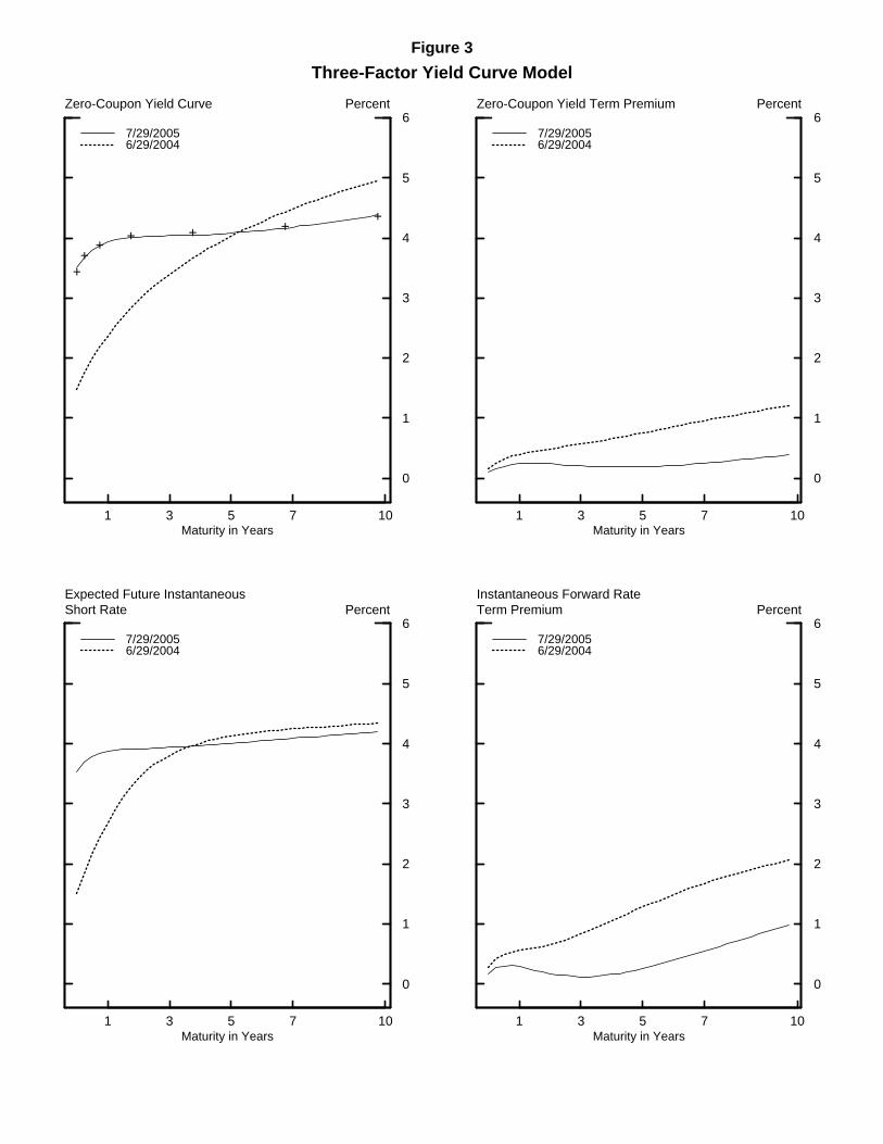
The top left panel of Figure 3 shows the fitted zero-coupon yield curve on two dates: June

29, 2004, and July 29, 2005, and the top right panel shows the schedule of associated

zero-coupon term premiums on these two dates, with these estimates derived from the

model described in the previous section. Over this time period, the ten-year zero-coupon

yield fell 50 basis points, but the associated term premium is estimated to have declined

by about 80 basis points. Accordingly, the model estimates imply that if the term

premium had not changed, ten-year yields would have risen modestly over this time

period, as one would expect in an environment of monetary policy tightening.

The decline in yields since the FOMC began tightening monetary policy in June

2004 is more stark when viewed in terms of instantaneous forward rates. The bottom two

panels of Figure 3 show the model-implied expectations of future short-term rates on

June 29, 2004, and July 29, 2005, and the schedule of associated instantaneous forward

term premiums on these two dates. Over this time period, near-term expected future

instantaneous interest rates rose. Part of this reflects the tightening of monetary policy

that was anticipated in June 2004, and part of it reflects a firming of policy expectations

since then. Distant-horizon expected future short-term interest rates fell slightly. But the

ten-year instantaneous forward rate declined 150 basis points over this time period, and

12

the model attributes most of this to a fall in the term premium as the ten-year

instantaneous forward rate term premium is estimated to have fallen 120 basis points.

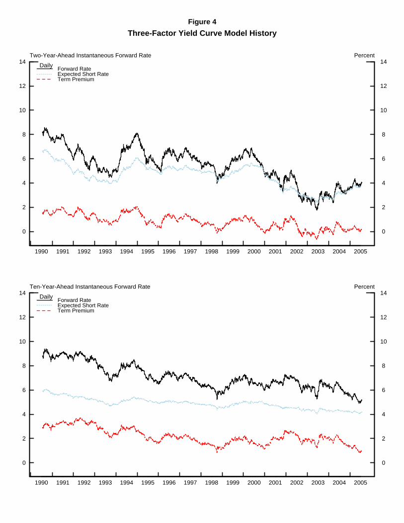
Figure 4 shows the time series of two- and ten-year-ahead instantaneous forward

rates, decomposed into estimated term premium and expected short-rate components. As

can be seen, the estimated ten-year instantaneous forward term premium has been

generally trending lower since 1990 and, with the recent fall since the middle of last year,

now stands below its historical range. Some other patterns in the historical estimated

term premiums are also noteworthy. In 1994, as the FOMC was raising rates, estimated

term premiums actually increased, in contrast to the recent experience. Estimated term

premiums dipped lower in October 1998, perhaps owing to "flight-to-quality" demand for

Treasury securities. The estimated ten-year instantaneous forward term premium rose

somewhat during and immediately after the two most recent recessions, consistent with

much of the literature on term premiums and the business cycle (e.g. Fama (1990)).

3.1 Relationship to Some Other Term Premium Estimates.

This three-factor arbitrage-free term structure model uses historical interest rate data and

an assumption that bonds are priced in a way that is internally consistent to parse today's

yield curve into a trajectory of expected future short-term interest rates and a schedule of

term premiums. It does not, however, make transparent why the model predicts smaller

term premiums now than it did one year ago. Recently Cochrane and Piazzesi (2005)

estimated bond term premiums by regressing excess bond returns on the term structure of

forward rates, where the excess bond returns are the returns on holding an n-year bond

over those on holding a one-year bond, for a holding period of one year. This gives a

13

very transparent link between changes in expected future bond returns and changes in the

term structure of forward rates—they found that the same tent shaped function of forward

rates could explain up to 44 percent of the variation in excess bond returns of different

maturities. The correlation between our estimate of the ten-year instantaneous forward

term premium and the return forecasting factor10 of Cochrane and Piazzesi is 0.83,

indicating that these two term premium measures are quite closely associated.

A very crude term-premium proxy that some have proposed is the spread between

the one-year forward rate ending four years hence and the one-year forward rate ending

five years hence. Some argue that monetary policy expectations might be fairly flat

between four and five years hence, and accordingly that the slope of the forward curve

may be mainly a reflection of the slope of the forward term premium. If the forward term

premium were moreover approximately linear, then this would give an approximation to

the expected excess returns on bonds of all maturities. We believe that the level and slope

of the distant-horizon forward curve reflects some combination of the trajectory of future

expected real rates, expected inflation, and term premiums and are skeptical of any

research that starts from an a priori assumption that movements in the forward curve at

distant horizons must reflect changes in just one of these three components. Nonetheless,

we agree that it is likely that the slope of the distant-horizon forward curve is affected by

term premiums among other things. The correlation between our estimate of the ten-year

instantaneous forward term premium and this term premium measure is 0.27.

We estimated the model of Cochrane and Piazzesi (2005), using Fama-Bliss

yields spliced onto data from the Svensson curve that is fitted to off-the-run Treasury

10 That is, -3.24-2.14f1+0.82f2+3.00f3+0.80f4-2.08f5 where fn denotes the one-year forward rate ending n years hence, estimates taken directly from Cochrane and Piazzesi (2005).

14

coupon securities at the Federal Reserve Board. This also indicates that expected excess

returns on longer maturity bonds have substantially declined since June 2004. Also, the

spread between the one-year forward rates ending four and five years hence has declined

from over 40 basis points just before the June 2004 FOMC meeting to about 10 basis

points in late July 2005.

3.2 Implications of the Stationarity of the Factors.

This three-factor arbitrage-free term structure model has the feature that so long as the

factors are stationary (all eigenvalues of K are negative), the forecasts of the factors will

always eventually converge to zero as the horizon goes to infinity. Thus the forecast of

the future instantaneous short rate at a sufficiently long horizon must converge to 0ρ .

Thus, movements in sufficiently distant-horizon instantaneous forward rates will always

be attributed exclusively to time-varying term premiums.11 This feature of the model,

while shared with all other arbitrage-free factor term structure models with stationary

factors (including stationary models with Markovian regime switching), seems somewhat

unrealistic. However, particularly when survey data are incorporated, the point at which

the forecast of the future instantaneous short rate asymptotes is well beyond the

maturities that we are considering in this paper.

11 Of course, the estimation method does not impose that the eigenvalues of K have to be negative, but in small samples, even if some eigenvalues of the K are zero in population, the probability is high that all three eigenvalues of the estimated K matrix will be negative (the analog of the usual downward small-sample bias in estimating an autoregression).

15

4. An Extension Incorporating Inflation.

In section 2, we gave expressions relating the price of a real bond to a real pricing kernel

(equation (3)) and of a nominal bond to a nominal pricing kernel (equation (4)). The real

pricing kernel, ( )Rm t , is equal to the nominal pricing kernel, ( )m t , multiplied by the

price level, ( )Q t . We do not observe prices of real bonds, other than prices of Treasury

Inflation Protected Securities (TIPS) which have only been trading since late 1997 and

which had evidently large liquidity premiums in the years shortly after their inception,

and which are not used in the models discussed in this paper. But we do observe inflation

data, and can combine inflation data and nominal yields data to price synthetic real

bonds. Other papers that have constructed real term structure models from inflation and

nominal yields data include Ang and Bekaert (2005).

The model of the real term structure described in this paper is due to Kim (2004).

The key extra feature that allows the model to price real bonds is to assume a

specification that relates inflation to the factors. It is assumed that equations (3), (4), and

(5) hold and that

0( ) ( ) ( ) ' ( )

( )dQ t t dt dW t dB tQ t

π σ σ= + + (9)

( ) ( ) ( ) ' ( )( )

dm t r t dt t dB tm t

λ= − −

0( ) ' ( )t x tπ μ μ= +

'0( ) ( )r t x tρ ρ= +

and ( ) ( )t x tλ φ= + Φ

16

where 0μ , 0ρ , and 0σ are constants, μ , ρ , σ , and φ are 3x1 vectors, Φ is a 3x3

matrix and ( )W t is a standard Brownian motion that is independent of ( )B t . Equation

(9) can be interpreted as implying that inflation is the sum of expected and unexpected

components and that the latter is driven by some combination of the Brownian motions in

(5) and by a fourth independent Brownian motion. Apart from the specification for

inflation, the model is identical to the nominal term structure model discussed earlier.

Kim (2004) shows how this gives a model that can be written in state space form in

which inflation, nominal yields and survey expectations12 are the observed data and the

latent factors ( )x t are the state variables. This provides a four-way decomposition of

yields into expected future real rates, expected future inflation, a real term premium, and

an inflation risk premium that is defined as the difference between nominal and real term

premiums. The model is estimated using weekly data over the sample period from 1990

to July 2005, with inflation measured by total seasonally adjusted CPI.

5. Empirical Results from the Real Term Structure Model.

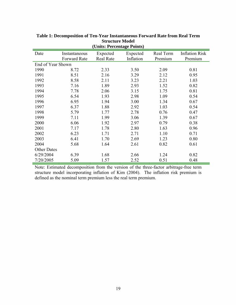
Table 1 shows the decomposition of the ten-year instantaneous forward rate into the

expected future real short rate ten years hence, expected future inflation ten years hence,

the real term premium and the inflation risk premium at the end of each year, using the

model described in the previous section. Results are also shown for June 29, 2004 and

for July 20, 2005.

12 In addition to the Blue Chip survey expectations of interest rates used as in the nominal term structure model, inflation survey expectations from the Survey of Professional Forecasters at one- and ten-year horizons are also incorporated. These are likewise treated as noisy measures of the true underlying latent inflation expectations (i.e. it is assumed that the survey measures of inflation expectations are equal to true inflation expectations plus Gaussian measurement error).

17

As can be seen in Table 1, long-horizon inflation expectations implied by the

model drifted lower over the 1990s from about 3½ percent at the end of 1990 to about 2½

percent in July 2005. The expected real rate also fell from 2¼ percent to about 1½

percent. Recall that inflation is measured by total CPI—to whatever extent that this is

likely to overstate inflation, the inflation expectation will be biased upwards and the real

rate biased downwards. Both the estimated real term premium and the inflation risk

premium have fallen, on net, since 1990.

Comparing the decomposition just before the June 2004 FOMC meeting with the

latest data, both expected future real rates and expected future inflation have edged lower

by about 10 basis points. The real term premium is estimated to have plunged from 125

basis points to 50 basis points. The estimated nominal term premium declined even

more, leaving the estimated inflation risk premium down about 30 basis points. The

nominal instantaneous ten-year forward term premium was estimated to be about 2

percent in June 2004, and more than half of this was parsed by the model to be the real

term premium. The nominal instantaneous ten-year forward term premium is now

estimated to be down to about 1 percent, about evenly split between real and inflation

premiums.

6. Conclusions and Future Work.

This paper has described a three-factor arbitrage free nominal term structure model

(Duffee (2002) and Kim and Orphanides (2004)) and an extension to incorporate inflation

(Kim (2004)). Judging from these models, the phenomenon of falling long-term yields

and distant-horizon forward rates since before the June 2004 FOMC meeting owes to

18

declining term premiums. In the real term structure model, real term premiums are

estimated to have fallen by about two-thirds as much as nominal term premiums, leaving

inflation risk premiums down about 30 basis points.

We have not reported standard errors associated with estimates of term premiums

and expected future short rates, but we see no special difficulty in computing bootstrap

standard errors. It would also be interesting to fit a model imposing that one of the

factors be nonstationary, as this would allow the point at which the expected future short-

rate asymptotes to vary over time, as discussed in subsection 3.2. Although the real term

structure model described here does not incorporate TIPS data, it is possible to include

TIPS yields, specifying that the TIPS yields, where available, are equal to the

unobservable synthetic real yields less an unobservable liquidity premium. These topics,

among others, are the subject of ongoing and future research on the term structure by

Federal Reserve Board staff.

19

Table 1: Decomposition of Ten-Year Instantaneous Forward Rate from Real Term

Structure Model (Units: Percentage Points)

Date Instantaneous Forward Rate

Expected Real Rate

Expected Inflation

Real Term Premium

Inflation Risk Premium

End of Year Shown 1990 8.72 2.33 3.50 2.09 0.81 1991 8.51 2.16 3.29 2.12 0.95 1992 8.58 2.11 3.23 2.21 1.03 1993 7.16 1.89 2.93 1.52 0.82 1994 7.78 2.06 3.15 1.75 0.81 1995 6.54 1.93 2.98 1.09 0.54 1996 6.95 1.94 3.00 1.34 0.67 1997 6.37 1.88 2.92 1.03 0.54 1998 5.79 1.77 2.78 0.76 0.47 1999 7.11 1.99 3.06 1.39 0.67 2000 6.06 1.92 2.97 0.79 0.38 2001 7.17 1.78 2.80 1.63 0.96 2002 6.23 1.71 2.71 1.10 0.71 2003 6.41 1.70 2.69 1.23 0.80 2004 5.68 1.64 2.61 0.82 0.61 Other Dates 6/29/2004 6.39 1.68 2.66 1.24 0.82 7/20/2005 5.09 1.57 2.52 0.51 0.48 Note: Estimated decomposition from the version of the three-factor arbitrage-free term structure model incorporating inflation of Kim (2004). The inflation risk premium is defined as the nominal term premium less the real term premium.

20

References

Ahmed, Shaghil, Andrew Levin and Beth-Anne Wilson (2002), “Recent U.S.

Macroeconomic Stability: Good Policies, Good Practices, or Good Luck?,” International

Finance Discussion Paper 730, Board of Governors of the Federal Reserve System.

Ang, Andrew and Geert Bekaert (2005), “The Term Structure of Real Rates and

Expected Inflation,” working paper, Columbia University Graduate School of Business.

Bernanke, Ben, Vincent Reinhart, and Brian Sack (2004), “Monetary Policy Alternatives

at the Zero Bound,” Brookings Papers on Economic Activity, 2, pp.1-100.

Cochrane, John (2001), Asset Pricing, Princeton University Press, Princeton, New Jersey.

Cochrane, John and Monika Piazzesi (2005), “Bond Risk Premia,” American Economic

Review, 95, pp.138-160.

Duffee, Gregory (2002), “Term Premia and Interest Rate Forecasts in Affine Models,”

Journal of Finance, 57, pp.405-443.

Duffie, Darrell and Rui Kan (1996), “Yield Factor Models of Interest Rates,”

Mathematical Finance, 64, pp.379-406.

Fama, Eugene (1990), “Term-structure Forecasts of Interest Rates, Inflation and Real

Returns,” Journal of Monetary Economics, 25, pp.59-76.

Kim, Don (2004), “Inflation and the Real Term Structure,” working paper, Board of

Governors of the Federal Reserve System.

Kim, Don and Athanasios Orphanides (2004), “Term structure estimation with survey

data on interest rate forecasts,” working paper, Board of Governors of the Federal

Reserve System.

21

Langetieg, Terence (1980): “A Multivariate Model of the Term Structure,” Journal of

Finance, 35, pp.71-97.

McConnell, Megan and Gabriel Perez-Quiros (2000): “Output Fluctuations in the United

States: What has Changed Since the Early 1980s,” American Economic Review, 90,

pp.1464-1476.

Rudebusch, Glenn and Tao Wu (2003), “A Macro-Finance Model of the Term

Structure, Monetary Policy, and the Economy,” Working Papers in Applied Economic

Theory, Federal Reserve Bank of San Francisco.

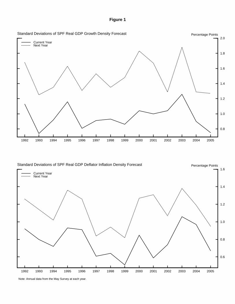
Figure 1

Note: Annual data from the May Survey at each year.

1992 1993 1994 1995 1996 1997 1998 1999 2000 2001 2002 2003 2004 2005

0.8

1.0

1.2

1.4

1.6

1.8

2.0Percentage Points

Current YearNext Year

Standard Deviations of SPF Real GDP Growth Density Forecast

1992 1993 1994 1995 1996 1997 1998 1999 2000 2001 2002 2003 2004 2005

0.6

0.8

1.0

1.2

1.4

1.6Percentage Points

Current YearNext Year

Standard Deviations of SPF Real GDP Deflator Inflation Density Forecast

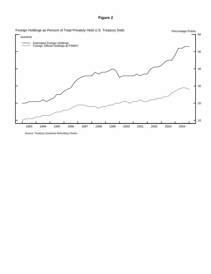
Figure 2

1993 1994 1995 1996 1997 1998 1999 2000 2001 2002 2003 2004

10

20

30

40

50

60Percentage Points

Estimated Foreign HoldingsForeign Official Holdings at FRBNY

Foreign Holdings as Percent of Total Privately Held U.S. Treasury Debt

Source: Treasury Quarterly Refunding Charts.

Quarterly

1 3 5 7 10

0

1

2

3

4

5

6Zero-Coupon Yield Curve Percent

7/29/20056/29/2004

Maturity in Years

++

++ + +

+

1 3 5 7 10

0

1

2

3

4

5

6Zero-Coupon Yield Term Premium Percent

7/29/20056/29/2004

Maturity in Years

1 3 5 7 10

0

1

2

3

4

5

6

Expected Future InstantaneousShort Rate Percent

7/29/20056/29/2004

Maturity in Years1 3 5 7 10

0

1

2

3

4

5

6

Instantaneous Forward RateTerm Premium Percent

7/29/20056/29/2004

Maturity in Years

Figure 3

Three-Factor Yield Curve Model

0

2

4

6

8

10

12

14

1990 1991 1992 1993 1994 1995 1996 1997 1998 1999 2000 2001 2002 2003 2004 2005

0

2

4

6

8

10

12

14Two-Year-Ahead Instantaneous Forward Rate Percent

Forward RateExpected Short RateTerm Premium

Daily

0

2

4

6

8

10

12

14

1990 1991 1992 1993 1994 1995 1996 1997 1998 1999 2000 2001 2002 2003 2004 2005

0

2

4

6

8

10

12

14Ten-Year-Ahead Instantaneous Forward Rate Percent

Forward RateExpected Short RateTerm Premium

Daily

Figure 4

Three-Factor Yield Curve Model History