an empirical test of factor likelihood arbitrage pricing ... · pdf filean empirical test of...

European Journal of Accounting Auditing and Finance Research

Vol.1, No.4, pp.95-114, December 2013

Published by European Centre for Research Training and Development UK(www.ea-journals.org)

95

AN EMPIRICAL TEST OF FACTOR LIKELIHOOD ARBITRAGE PRICING THEORY

IN NIGERIA

Arewa, Ajibola

Lagos State University, Lagos, Nigeria.

Faculty of Management Sciences,

Department of Accounting and Finance.

Nwakanma Prince C

University of Port-Harcourt, River State, Nigeria

Faculty of Management Sciences,

Department of Finance and Banking.

ABSTRACT: The study employs the Principal Component Analytical (PCA) technique to derive

proxies for the factor likelihood APT of Rose using monthly security returns of 53 companies

listed in NSE over the period 1 Jan 2003 to 31 Dec 2011. The results of the PCA methodology

reveal that 17 latent factors are identified in the Nigerian equity market; while the estimated

results of the cross-sectional APT pricing model show that only 4 of the factors are priced.

However, the evidence of systematic hypothesis is not ascertained in this study. Thus, the

unsystematic risk associate with arbitrage portfolios in the market cannot be reduced/ eliminated

no matter the level of diversification.

KEYWORDS: Latent factors, APT, Idiosyncratic risk, Diversification, Arbitrage Portfolios,

PCA

Jel Code: C4; D4; D8; E4; G1

INTRODUCTION

The foundational works on asset pricing models begin with the development of the Capital Asset

Pricing Model (CAPM) by (Shape, 1964) and late (Lintner, 1965). The CAPM is a single factor

model whose empirical testability hinged on the market portfolio but the argument that the true

market portfolio cannot be inspected poses serious limitation to the acceptability of the model.

Thus, Ross (1976) argues persuasively that since the market portfolio is not identifiable the

CAPM has never been tested and never will it be. Roll (1977) extended the criticisms up to the

point of rejecting the CAPM completely and becomes the ardent supporter of the Ross’ (1976)

Arbitrage Pricing Theory (APT). The APT is an elegant model with two pricing identifications.

The earlier one is called factor likelihood APT (FLAPT) while the later one is referred to pre-

specified macroeconomic variables APT (PMVAPT). The PMVAPT shows a relationship

between expected return and a set of randomly selected macroeconomic variables. In an equal

token, the FLAPT provides intuitive linear relationship between expected return and




96

asymptotically large latent factors. However, the focus of this study is directed to the FLAPT

which is proposed, developed and introduced to the frontier of core Finance by (Ross, 1976) and

(Ross & Roll, 1977).

Ross’ empirical proof of the FLAPT model is an indication that the linearity assumption of the

model is a necessary condition to attain equilibrium in a market where investors arbitrage to take

advantage of price differentials in order to maximize their utilities. Therefore, investors hold

arbitrage portfolios that allow them to maximize return by varying the proportions of their assets

but leaving the total investable income unchanged. The latent factors attached to these portfolios

are the covariance risks which are measures of risk factors investors cannot eliminate/reduce

through diversification. The popular opinion of the FLAPT is that the latent factors or the

unobservable market factors explain variations in asset return better than the CAPM beta factor;

therefore in an ideal capital market their some risk factors which investors cannot observe yet

they command risk premium. The empirical testability of the FLAPT right from inspection

begins with the work of (Gehr, 1975). He employs principal components analysis (PCA) method

to extract the common factors and then regresses them against average return and finds that only

one factor is significant in explain asset return while Ross and Roll’s (1980) test provides

evidence for three priced factors. In a recent time, Mohseni (2007), Tursoy, Guisel and Rjoub

(2008) examine the empirical validity of the FLAPT model and find that the pricing

identification of this model suffices to explain average return very well; even Subramanyam

(2010) has made important contribution. The beauty of this model is that it helps to reveal the

market risks that cannot be identified using the CAPM and its subsequent versions. Hence, a

market that has not been subjected to FLAPT test will undoubtedly leave its participants to be

completely unaware of un-diversifiable latent risks.

Our survey of literature has revealed that much of the works on the FLAPT are centered on

advanced and Asian emerging countries neglecting most of the African nations particularly

Nigeria. Several studies such as Asaolu and Ogunmuyiwa (2011), Izedonmi and Abdullahi

(2011) have made attempts in Nigeria to shrink this gap but they fail to subject their studies to

two-pass regression technique. Also, their studies are only based on macroeconomic variables

and therefore do not incorporate the contracting tests. In the spirit to ameliorate this egregious

shortcoming, we are motivated to price the FLAPT identification in Nigerian stock market with

the aim of determining the number of the latent factors that investors cannot avoid no matter the

level of their diversification. However, the outline for this study is organized as follows: section

1 introduction which we have already discussed, section 2, reviews the prior literature works of

some selected authors, section 3, describes the methodology and data; while empirical findings,

concluding remarks and recommendations are respectively presented in sections 4,5,& 6.

LITERATURE REVIEW

Ross’ (1976, 1977) Arbitrage Pricing Theory (APT) provides an alternative theoretical pricing

model to the CAPM from which a partial equilibrium asset pricing model could be obtained.

Even though the APT celebrates the intuitive simplicity of linearity between returns and

unobservable or observable market factors, yet it does not expressly follow quadratic relationship

or mean-variance efficient feature of the CAPM for return distributions in any stock market.




97

These undoubtedly lead to some pertinent merits as follows: Roll's criticisms are plausibly

reasonable since the market portfolio is not directly incorporated in the equilibrium pricing

models. Also, an ex ante APT pricing model rests on relatively weak/few assumptions, lastly, the

one-factor APT framework now serves as a benchmark in which the existing findings on the tests

of the CAPM can be re-interpreted. The derivation of the APT pricing equation is rooted on two

major assumptions: firstly, that there is perfect competition in the capital markets and secondly,

that investors are rational economic agents who always prefer more wealth to less wealth under

the context of certainty. Thus, according to (Ross, 1976, 1970), even (Hubermann, 1980) and

(Chen, 1980), the return generating process of the APT specification can be expressed as:

Ri = CO + βiδi + βjδp +…. + ej …………………………….. (1)

Where:

Rj is the return on security i

βi is defined as the sensitivity of security i to movements in the common

factor δj

E(ej) = 0;

Cov(δi,ej) = 0;

Cov(ei,ej) = 0;

Var(ei) = δ2 < ∞;

It is theoretically assumed that investors consider all assets in a capital market as a set of

arbitrage portfolios, which give them opportunity to rationalise their wealth across array of

competitive stocks but their total wealth remained unchanged. Thus, arbitrage portfolios are

perfectly diversified portfolios with zero non-systematic risk. Assuming the weights of the

portfolios securities are chosen such that the systematic risk is also zero, then it means that each

of these portfolios must exhibit zero total risk. This also involves zero net wealth which must

earn zero expected return in equilibrium suppose there are no arbitrage opportunities. Ross

(1976) critically observed that if returns are generated by equation (1), then a pricing equation

such as (2) can directly follow from the orthogonality of risk and return of investment

proportions.

Ri = CO + λ1βi1 + λ2βi2 ... + λpβip …………………………….(2)

C0 = constants

λ1 = 1, 2... p

Equation (2) states that the expected return on any asset is linearly related to the sensitivity or

covariance of the asset return with the p common factor. Hence, there is a functional similarity

between equations (1&2), and if p = 1 then, the CAPM and APT have identical pricing

implications. However, to derive equation (2), Ross (1976) did not follow the assumption of

mean-variance sufficiency for either return distributions or utility functions. Also, it is clear that

the market portfolio does not play a central role in the formulation of the APT pricing equation.

It is also worth mentioning that the APT and CAPM are distinguished solely on the basis of the

generality of the return generating process in respect of each of the pricing equations. Stapleton

and Subrahmanyam (1980, p.9) argued that "... Given a linear underlying structure of returns, the

only distribution that permits linear regression with constant variance is the normal distribution".

It implies that multivariate normality would be a required assumption for the APT to hold. Ross

(1976) explicitly specified that a large number of assets exist and the specification errors losses

sufficient independence, therefore the error terms converge to zero in arbitrage portfolios. If the

errors fail to converge to zero in arbitrage portfolios, then the orthogonality arguments leading to




98

equation (2) do not stand. Literature survey has shown a clear picture that experimental design of

the APT is still emerging and hence relatively few empirical tests of the APT have been

performed to date. Also, some of these tests are centered in advanced markets of American,

European, emerging Asian countries and very few studies are carried out in African countries.

Obviously, the tests of the APT are conducted on the individual securities returns rather than

groups and then the factor analytic techniques are employed to derived proxies for the APT

factor risk. Based on these two steps measured above, Gehr (1975) collected 30 years monthly

securities’ returns data from the CRSP tape. He adoptes the principal components analysis (PCA)

method to extract the common factors and the factors are obliquely rotated. In the first step, he

regresses each industry index on the factor scores to extract the latent factors and their

correspondent loadings. In the next step, he conducted Cross Sectional OLS regression to obtain

the estimate of the coefficients in the APT model. His results show that only one factor appeared

to be significantly priced over the complete 30 years period of investigation. We note that Gehr’s

empirical ground was not tested against a specified alternative and therefore, lack empirical

power to separate the CAPM from the APT. Also, Gehr’s work lack power for several other

reasons- one the factor solutions are arbitrarily rotated to one of a large number of acceptable

solutions leading to strong multicollinearity among the explanatory variables in the second stage

of his experiment and hence, the difficulties of interpreting t-statistics on the explanatory

variables are ignored. Two, the explained variables in his experimental design are average

(mean) returns on industry indices instead of individual securities’ returns. This places an

implicit limitation to his experimental design on APT test. Finally, he does not make attempt to

deal with the errors in variables in the cross sectional OLS regressions used and as such, the

estimated risk premia are grossly biased. Roll and Ross (1980), otherwise known as RR have

been seen to have performed the most compressive test of the APT to date. They are able to

overcome the first and second deficiencies of Gehr’s test but their cross sectional pricing tests

still fall victims of the errors in variables. In the study of RR, about 42 groups of 30 securities

each quoted in NYSE were alphabetically selected to cover a period of July 3 1962 to December

31 1972. They conduct the following experiments for each of the groups using daily arithmetic

returns adjusted for all capital changes and dividend payments.

i. They compute the covariance matrix for the time series sample for each of the group of 30

securities covering the period of their analysis

ii. They employ Maximum Likelihood Factor Analysis (MLFA) technique to extract the number of

factors and the corresponding factor loadings.

iii. Finally, they regress the factor loading matrix on the average securities returns to provide

estimates of the factor risk premia which are evaluated for significance.

In order to test for the validity of the systematic risk hypothesis, they repeat the cross sectional

regression by importing the standard deviation of returns into the APT model. Hence, the

explanatory variables are now the estimates of the factor loadings and the standard deviation of

returns. Their results indicate that out of the four factors being priced cross sectionally, three

factors are significantly priced. Thus, their findings provide a support to APT and empirically

distinguish it from the CAPM on the basis of the pricing equation. Brown and Weinstein (1981)

attempt to replicate part of Roll and Ross’ (1980) empirical findings based on an alternative

method. They discover that a 5 factor return generating process is not evident in any of the




99

grouped securities. Also, the cross-sectional pricing results indicate that the average returns are

not consistent with the APT framework for the five or even fewer factors. They finally note that

their results are slightly sensitive to normality due to the surprising sensitivity of the APT

evidence to the test method or methodology. Reinganum (1980) also uses alternative

methodology to test the APT’s validity over time. His test requires that the APT explains the size

anomaly which arises from the market efficiency studies that use the equilibrium market model.

However, it is noted that Reinganum could not resolve the problem of size anomaly using the

APT methodological framework. Even, it is discovered that the use of more complex return

generating model does not do better than the parsimonious one factor model related to CAPM.

Connor and Korajczyk (1986) employ the Principal Component Analysis (PCA) proposed by

(Chamberlain & Rothchild, 1983) and document five factors explaining the asset returns.

Kryzanowski and To (1983) tested APT on the Canadian data and discover that on the average,

the number of factors explaining returns remain approximately the same across various samples

of the same size and across various time intervals, except that the numbers of significant factors

increase with group size. Dhankar and Esq (2005) analyze APT in the Indian stock market using

monthly and weekly returns for the period, 1991-2002 and show that the APT with multiple

factors provides a better explanation of risk- return relationship than CAPM which used beta as

the single measure of risk. Mohseni (2007) applies the APT on selected firms in the Tehran

Stock Exchange (TSE) using the (Fama & Macbeth`s 1973) methods. The two risk factors are

measured for these groups of firms (money supply and oil price) and the sensitivity of each

firm’s return is estimated by the two factors and documentes that APT model is significant in

explaining the returns on his selected sample of firms. Tursoy, Guisel and Rjoub (2008)

empirically examine the validity of the APT in Istanbul Stock Exchange (ISE) using monthly

security returns data that ranged from February 2001 to September 2005 and found that stock

returns are influenced by different systematic factors as opposed to the claims of the CAPM.

Subramanyam (2010) reviewed the literature on cross-section of expected stock returns for the

past twenty-five years and drew the following conclusions. Too many predictive variables were

used without a proper analysis of their correlation structure which might give rise to the presence

of multi-collearity. Hence, generally speaking these studies lack the ability to account for control

of variables imported in the APT framework. Wang et, al (2011) re-modify the classical FLAPT

and provide overwhelming evidence in support of the model as a good benchmark for explaining

stock return. Pooya et, al (2011) carry out an empirical test of the APT in the Iranian stock

market over a period 1991 to 2008 using the principal component analysis and canonical

correlation model which show that at least one to three factors can explain the cross-section of

expected returns in this market and they document that financial and economical sanctions

possibly explain the negative stock market returns which reflect the reaction of investors to the

announcement of sanctions. In general, their findings reveal a weak applicability of APT in this

market. Florin (2012) investigates the factor that influence stock return in Romanian stock

market over six year time span ranging from first January 2005 to thirty-first December 2010

using APT framework and documents that four to six factors are significant in explaining asset

return in this market.

METHODOLOGY




100

The factor likelihood APT pricing model adopted in this study takes its leads from the a-priori

works of Ross (1976), Ross and Roll (1977) and it is stated as follows in a modified form:

rit = y0 + y1bî1 + y2b

î2 +……….. + ykb

îk + e

~i………………(1)

Where: ri is the average return of i`th securities

bi1, bi2……..bik are the estimated factor loadings

y1, y2………….yk are the estimated risk premia associated with the i`th factors.

y0 and e~

i are the constants and error terms respectively.

Thus, the first APT hypothesis is tested when equation (1) is estimated and the numbers of

parameters that are significant are known. A-priori demands that if at least one of the parameters

is significant, it means that APT is empirically fair. To test the second hypothesis that the

standard deviation of return does not command a premium in addition to the factor risk

coefficients; we have to obtain the residuals from equation (1) and then make them the explained

variables in the following regression:

e~

i = λ0 + λ1S^r~

i + W~

I ………………………(2)

Where: S^r~

i is the estimated standard deviation of returns calculated over the same period as the

factor loading estimates in equation (1). On the a-priori ground E(λ1) = 0 meaning that the

estimate of the standard deviation of return is not expected to be statistically significant. If this a-

priori ground holds, it means that the systematic risk hypothesis that the only risk that commands

premium is the systematic risk is valid.

The principal component factor model is essentially used for deriving proxies for the bi’s in

equation 1, and it has the following forms:

x~

i = bi1F~

1 + bi2 F~

2 + ………. + bim F~

m + eiµ~

i ……….(3)

i = 1, 2, 3 ……p

Where: Xj = is the observed variables (i. e. security returns)

bji's are the systematic risk estimates associated with the

representative common factors and they are (P x M) matrices

F's are the (M x 1) random vector of M common factors.

µj is a (P x P) diagonal matrix, called the unique factor pattern.

x is an (M x 1) random vector of P unique factors, while M and

P is the number of factor extracted and number of security respectively.

Thus, in a matrix form equation 3 can be restated as follows:

x~

i = E(x~

i) + ΒF + µy………………………………………….(4)

Where: E(x~

i) is the expected security return.

β is the systematic risk factors

µy is the idiosyncratic risk

If E(F) = 0, E(µy) = 0 and E(Fµy) = 0; the beta (β) matrix is given as:

β = E[x~

i – E(x~

i)F1] [E(FF

1)-1

] ………………………………………….(5)

Equation 5 is defined as a standard linear projection where xi is the vector of asset return and F is

a vector of zero-mean variates. The linear projection has divided the returns into expected returns

which correlate with F and zero-mean idiosyncratic factor which is uncorrelated with F. This

shows evidence that the risk factors in equation (4) are not diversifiable but the idiosyncratic risk

can be diversified.

In the strict Factor Models, it is arguably true that the systematic factor risks and specific or

idiosyncratic risks are uncorrelated, and as such the covariance matrix of securities’ returns

(COV) which is given as E[(x~

i – E(x~

i)) (x~

i – E(x~

i))1] can be expressed as the sum of the




101

covariance matrix of each security’s systematic risk factor and covariance matrix of the

idiosyncratic risk. Thus:

COV = βE[FF1]β

1 + W…………………………………………(6)

Where:

W = E(µyµy) …………………………………………(7)

Since the idiosyncratic returns are assumed to be uncorrelated with one another, therefore, the

covariance matrix of the idiosyncratic risk (w) is referred to diagonal matrix. Of course, this

captures the essential feature of the strict factor model with undiversifiable covariance risks. It

has been contended that the strict factor model can only have empirical content if the number of

securities (k) is much less than number of observation (n). The empirical studies in US have k

within the range of 1 to 15 while n ranges from 1000 – 6000 depending upon the selection

criteria. Ross (1976) based his argument on the strict diagonality of the idiosyncratic risk (w) to

assert that this risk can be diversified away in a portfolio of many assets and as such it should

command no premium. Chamberlain (1983) and Chamberlain and Rothschild (1983) develop an

asymptotic statistical model for asset returns data known as approximate factor. This model

supports the diversifiability of the idiosyncratic risk but weakens the diagonality condition on W,

and it also presents a condition in which the factor risks are non diversifiable. In essence, the

Chamberlain and Rothschild’s approximate factor structure is defined as factor decomposition

where the µy’s are considered to be irrelevant but the F’s are pervasive. They persuasively

demonstrate that the condition of diversifiability is equal to a finite upper bound on the

maximum Eigen value of Wn as n tends toward infinity (α) and to a finite upper bound on the

minimum Eigen value βn and n goes to infinity (α). It is suggested by (Connoor & Korajczyk,

1993) that for an econometric work, introducing a mixing condition on the sequence of

idiosyncratic risk is more relevant than the bounded Eigen value condition alone.

Let us consider equation (3) with white noise once again; if the unique factors are removed, by a

priori the formal statement of this model becomes:

x~

i = bi2F1 + bi2F2 + ………………..bimFm ……………………..(8)

Equation (8) is a noiseless factor model that is it does not have idiosyncratic risk. This is rather

too strong a restriction on asset returns but it is useful for the intuition it provides. In this case an

exact arbitrage argument is sufficient for the APT. here, we do not need a large number of assets

and there is no approximate error in the APT pricing restriction (Ross (1977)). The need for a

priori adjustment of the correlation matrix relating to equation (8) has made the estimation of

communalities an important step in performing principal Factor Analysis (PFA); as a result the

number of estimation factors has been pointed to approximate the amount of communality for

any variable. Note, whist the PFA method requires initial estimates of communalities, maximum

Likelihood Factor Analysis (MLFA) techniques only demands on the number of common factors

(see, Harman 1976, p. 84-90). MLFA directly depends on the assumption that the sample

employed in a study is drawn from a multivariate normal distribution in which case the

distribution function of the covariance elements is known and the estimation of the factor scores

by maximum likelihood methods is then possible which is subject to an a priori specification of

the number of factor (Harman, 1976, p. 201).




102

Data

The data employed in this study are purely secondary data of raw stock prices and market indices

which are respectively sourced from NSE web-site: www.cscsnigerialtd.com. The data cover a

sampling period of Jan 2003 to December 2011. However, they are transformed to monthly stock

returns using logarithmic equation.

EMPIRICAL RESULTS

Generally, the tests of the APT’s validity hinge on two theoretical prepositions/hypotheses as

discussed in section three. However, since the empirical tests of the APT is linked with factor

theory, the authors present and discuss first, the results of the factor model in relation to the

version of the APT applied in this study before proceeding to test the pricing implication of the

APT.

Factor Results and Estimation

A procedure is followed prior to the estimation of the formal factor model stated in section 3 (i.e.

equation 3). This procedure includes: calculating the sample KMO and the individual security

KMO so as to determine the optimum sampling size on which the factor analysis can be carried

out. These steps are adherent to in this study and the results are discussed as follows:

Overall KMO Result

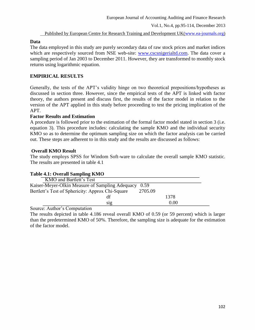
The study employs SPSS for Windom Soft-ware to calculate the overall sample KMO statistic.

The results are presented in table 4.1

Table 4.1: Overall Sampling KMO

KMO and Bartlett’s Test

Kaiser-Meyer-Olkin Measure of Sampling Adequacy 0.59

Bertlett’s Test of Sphericity: Approx Chi-Square 2705.09

df 1378

sig 0.00

Source: Author’s Computation

The results depicted in table 4.186 reveal overall KMO of 0.59 (or 59 percent) which is larger

than the predetermined KMO of 50%. Therefore, the sampling size is adequate for the estimation

of the factor model.

http://www.cscsnigerialtd.com/




103

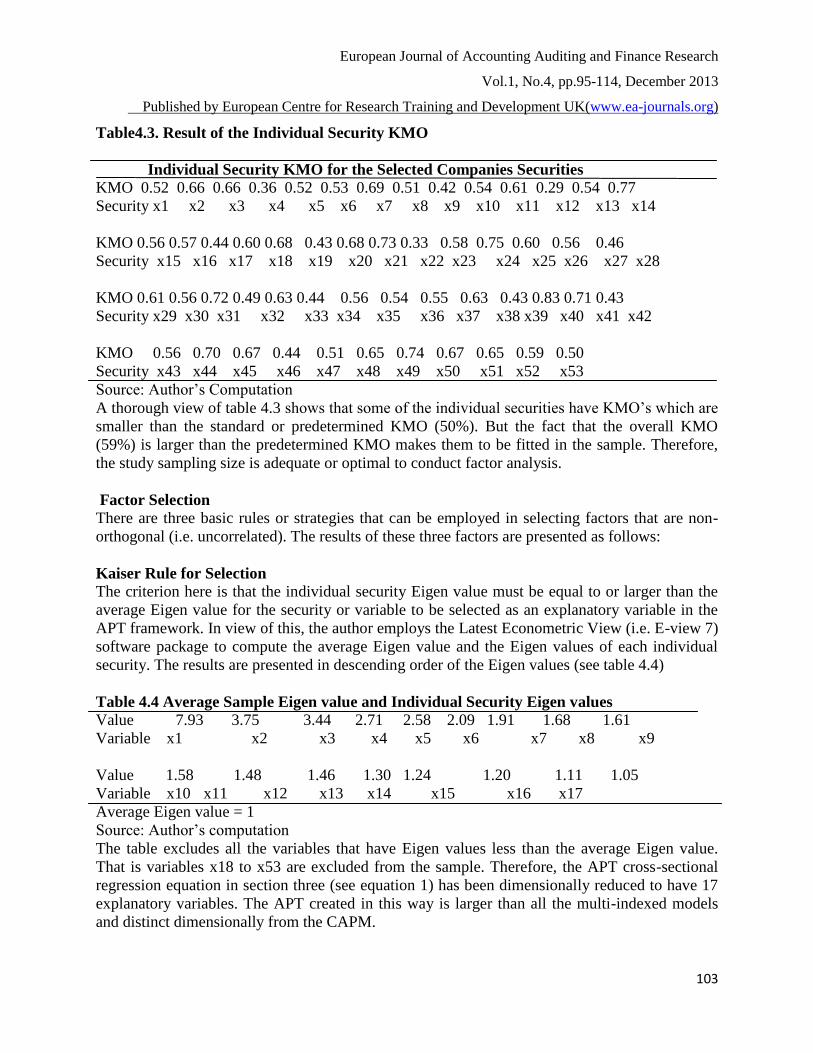
Table4.3. Result of the Individual Security KMO

Individual Security KMO for the Selected Companies Securities

KMO 0.52 0.66 0.66 0.36 0.52 0.53 0.69 0.51 0.42 0.54 0.61 0.29 0.54 0.77

Security x1 x2 x3 x4 x5 x6 x7 x8 x9 x10 x11 x12 x13 x14

KMO 0.56 0.57 0.44 0.60 0.68 0.43 0.68 0.73 0.33 0.58 0.75 0.60 0.56 0.46


KMO 0.61 0.56 0.72 0.49 0.63 0.44 0.56 0.54 0.55 0.63 0.43 0.83 0.71 0.43


KMO 0.56 0.70 0.67 0.44 0.51 0.65 0.74 0.67 0.65 0.59 0.50

Security x43 x44 x45 x46 x47 x48 x49 x50 x51 x52 x53


A thorough view of table 4.3 shows that some of the individual securities have KMO’s which are

smaller than the standard or predetermined KMO (50%). But the fact that the overall KMO

(59%) is larger than the predetermined KMO makes them to be fitted in the sample. Therefore,

the study sampling size is adequate or optimal to conduct factor analysis.

Factor Selection

There are three basic rules or strategies that can be employed in selecting factors that are non-

orthogonal (i.e. uncorrelated). The results of these three factors are presented as follows:

Kaiser Rule for Selection

The criterion here is that the individual security Eigen value must be equal to or larger than the

average Eigen value for the security or variable to be selected as an explanatory variable in the

APT framework. In view of this, the author employs the Latest Econometric View (i.e. E-view 7)

software package to compute the average Eigen value and the Eigen values of each individual

security. The results are presented in descending order of the Eigen values (see table 4.4)

Table 4.4 Average Sample Eigen value and Individual Security Eigen values

Value 7.93 3.75 3.44 2.71 2.58 2.09 1.91 1.68 1.61

Variable x1 x2 x3 x4 x5 x6 x7 x8 x9

Value 1.58 1.48 1.46 1.30 1.24 1.20 1.11 1.05

Variable x10 x11 x12 x13 x14 x15 x16 x17

Average Eigen value = 1

Source: Author’s computation

The table excludes all the variables that have Eigen values less than the average Eigen value.

That is variables x18 to x53 are excluded from the sample. Therefore, the APT cross-sectional

regression equation in section three (see equation 1) has been dimensionally reduced to have 17

explanatory variables. The APT created in this way is larger than all the multi-indexed models

and distinct dimensionally from the CAPM.




104

Variance Explained Strategy

This is an arbitrary rule that considers the first factors that explain 70 to 80 percent of the

cumulative variance. The cumulative percentage of variance explained and the percentage of

variance explained by each factor/variable are presented in table 4.18

Table 4.5 Percentage of Individual Factor Variance and Cumulative Variance Factor x1 x2 x3 x4 x5 x6 x7 x8 x9

% of variance explained

by each factor 14.96 7.08 6.48 5.12 4.88 3.93 3.6 3.17 3.04

Cumulative % 14.96 22.04 28.53 33.65 38.52 42.46 46.06 49.23 52.27

Factor x10 x11 x12 x13 x14 x15 x16 x17

% of variance explained

by each factor 2.99 2.8 2.76 2.46 2.34 2.27 2.09 1.96

Cumulative % 55.25 58.06 60.81 63.27 65.61 67.88 69.97 71.16


Looking at table 4.5, it is seen that the proportion of variance explained by each factor declines

as the cumulative percentage variance increases. Arbitrarily, the authors decide to stop at the

seventeen factor because after that the proportion of variance contributed by successive factors

becomes infinite decimal or negligible. Thus, seventeen factors contribute about 71.16 percent

variance to the cumulative percentage variance of the sample. Based on this rule, seventeen

factors are also selected.

Cattell Rule for Selection This rule is based on the scree plot method as shown in figure 4.1

Figure 4.4: Scree Plot on Cattell Rule for Selection

A visual view of the curve on figure (4.1), shows that it descends slightly up to number 17 and

thereafter, it starts descending very sharply. This means that by this rule, seventeen factors can

0.6

0.7

0.8

0.9

1.0

1.1

1.2

2 4 6 8 10 12 14 16

Scree Plot: Observed Matrix




105

be extracted. Therefore, it seems that the three rules suggest that seventeen factors can be

selected to test the empirical stance of the APT in Nigerian capital market. These factors are

loaded using the Principal Component Analysis (PCA)

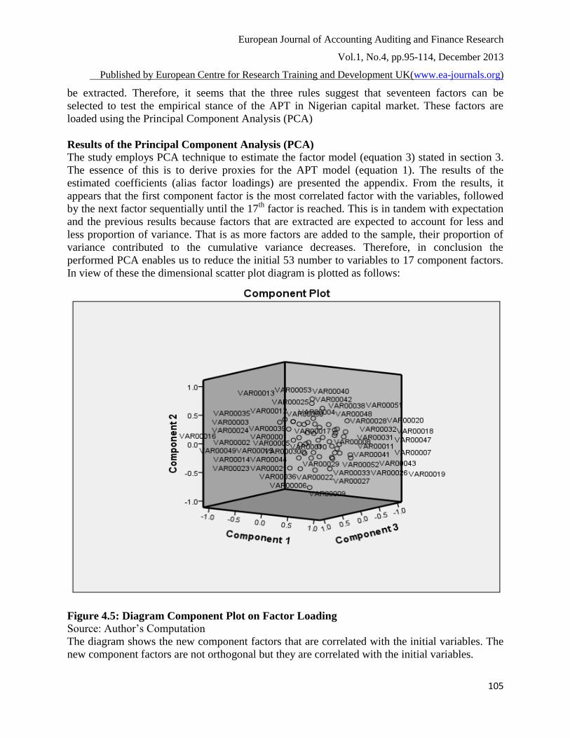
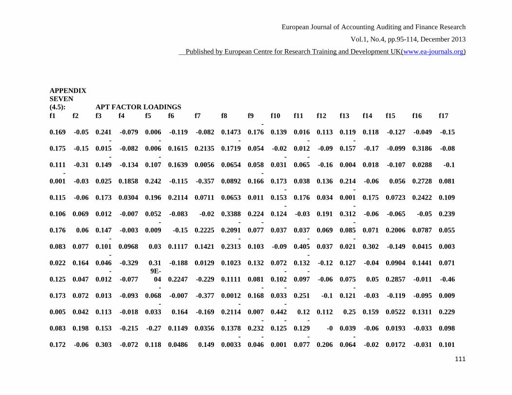
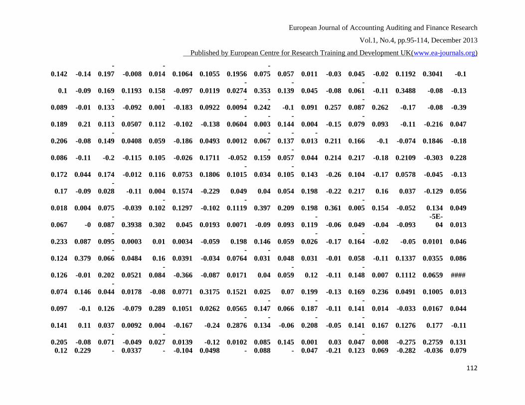
Results of the Principal Component Analysis (PCA) The study employs PCA technique to estimate the factor model (equation 3) stated in section 3.

The essence of this is to derive proxies for the APT model (equation 1). The results of the

estimated coefficients (alias factor loadings) are presented the appendix. From the results, it

appears that the first component factor is the most correlated factor with the variables, followed

by the next factor sequentially until the 17th

factor is reached. This is in tandem with expectation

and the previous results because factors that are extracted are expected to account for less and

less proportion of variance. That is as more factors are added to the sample, their proportion of

variance contributed to the cumulative variance decreases. Therefore, in conclusion the

performed PCA enables us to reduce the initial 53 number to variables to 17 component factors.

In view of these the dimensional scatter plot diagram is plotted as follows:

Figure 4.5: Diagram Component Plot on Factor Loading


The diagram shows the new component factors that are correlated with the initial variables. The

new component factors are not orthogonal but they are correlated with the initial variables.




106

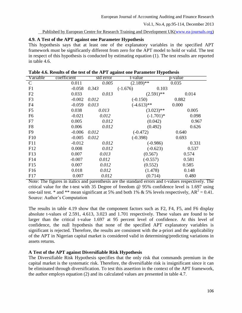
4.9. A Test of the APT against one Parameter Hypothesis

This hypothesis says that at least one of the explanatory variables in the specified APT

framework must be significantly different from zero for the APT model to hold or valid. The test

in respect of this hypothesis is conducted by estimating equation (1). The test results are reported

in table 4.6.

Table 4.6. Results of the test of the APT against one Parameter Hypothesis

Variable coefficient std error t-value p-value

C 0.011 0.005 (2.189)** 0.035

F1 -0.058 0.343 (-1.676) 0.103

F2 0.033 0.013 (2.591)** 0.014

F3 -0.002 0.012 (-0.150) 0.882

F4 -0.059 0.013 (-4.613)** 0.000

F5 0.038 0.013 (3.023)** 0.005

F6 -0.021 0.012 (-1.701)* 0.098

F7 0.005 0.012 (0.042) 0.967

F8 0.006 0.012 (0.492) 0.626

F9 -0.006 0.012 (-0.472) 0.640

F10 -0.005 0.012 (-0.398) 0.693

F11 -0.012 0.012 (-0.986) 0.331

F12 0.008 0.012 (-0.623) 0.537

F13 0.007 0.013 (0.567) 0.574

F14 -0.007 0.012 (-0.557) 0.581

F15 0.007 0.012 (0.552) 0.585

F16 0.018 0.012 (1.478) 0.148

F17 0.007 0.012 (0.714) 0.480

Note: The figures in italics and parenthesis are the standard errors and t-values respectively. The

critical value for the t-test with 35 Degree of freedom @ 95% confidence level is 1.697 using

one-tail test. * and ** mean significant at 5% and both 1% & 5% levels respectively, AR2 = 0.41.


The results in table 4.19 show that the component factors such as F2, F4, F5, and F6 display

absolute t-values of 2.591, 4.613, 3.023 and 1.701 respectively. These values are found to be

larger than the critical t-value 1.697 at 95 percent level of confidence. At this level of

confidence, the null hypothesis that none of the specified APT explanatory variables is

significant is rejected. Therefore, the results are consistent with the a-priori and the applicability

of the APT in Nigerian capital market is considered valid in determining/predicting variations in

assets returns.

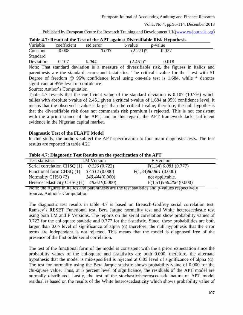
A Test of the APT against Diversifiable Risk Hypothesis

The Diversifiable Risk Hypothesis specifies that the only risk that commands premium in the

capital market is the systematic risk. Therefore, the diversifiable risk is insignificant since it can

be eliminated through diversification. To test this assertion in the context of the APT framework,

the author employs equation (2) and its calculated values are presented in table 4.7.




107

Table 4.7: Result of the Test of the APT against Diversifiable Risk Hypothesis Variable coefficient std error t-value p-value

Constant -0.008 0.003 (2.271)* 0.027

Standard

Deviation 0.107 0.044 (2.451)* 0.018

Note: That standard deviation is a measure of diversifiable risk, the figures in italics and

parenthesis are the standard errors and t-statistics. The critical t-value for the t-test with 51

Degree of freedom @ 95% confidence level using one-tale test is 1.684, while * denotes

significant at 95% level of confidence.


Table 4.7 reveals that the coefficient value of the standard deviation is 0.107 (10.7%) which

tallies with absolute t-value of 2.451.given a critical t-value of 1.684 at 95% confidence level, it

means that the observed t-value is larger than the critical t-value; therefore, the null hypothesis

that the diversifiable risk does not commands risk premium is rejected. This is not consistent

with the a-priori stance of the APT, and in this regard, the APT framework lacks sufficient

evidence in the Nigerian capital market.

Diagnostic Test of the FLAPT Model

In this study, the authors subject the APT specification to four main diagnostic tests. The test

results are reported in table 4.21

Table 4.7: Diagnostic Test Results on the specification of the APT

Test statistics LM Version F Version

Serial correlation CHSQ (1) 0.126 (0.722) F(1,34) 0.081 (0.777)

Functional form CHSQ (1) 37.312 (0.000) F(1,34)80.861 (0.000)

Normality CHSQ (2) 140.444(0.000) not applicable.

Heteroscedasticity CHSQ (1) 48.621(0.000) F(1,51)566.206 (0.000)

Note: the figures in italics and parenthesis are the test statistics and p-values respectively


The diagnostic test results in table 4.7 is based on Breusch-Godfrey serial correlation test,

Ramsey’s RESET Functional test, Bera Jarque normality test and White heteroscedastic test

using both LM and F Versions. The reports on the serial correlation show probability values of

0.722 for the chi-square statistic and 0.777 for the f-statistic. Since, these probabilities are both

larger than 0.05 level of significance of alpha (α) therefore, the null hypothesis that the error

terms are independent is not rejected. This means that the model is diagnosed free of the

presence of the first order serial correlation.

The test of the functional form of the model is consistent with the a priori expectation since the

probability values of the chi-square and f-statistics are both 0.000, therefore, the alternate

hypothesis that the model is mis-specified is rejected at 0.05 level of significance of alpha (α).

The test for normality using the Bera-Jarque statistic shows probability value of 0.000 for the

chi-square value. Thus, at 5 percent level of significance, the residuals of the APT model are

normally distributed. Lastly, the test of the stochastic/heteroscedastic nature of APT model

residual is based on the results of the White heteroscedasticity which shows probability value of




108

0.000 for both chi-square and f-statistics. Since this value is actually less than the 0.05 level of

significance of α, the null hypothesis that the variance of the residuals is constant is rejected.

Therefore, in the overall assessment the diagnostic test results reveal that the APT is fitted and

robust.

AUTHORS’ CONTRIBUTION TO KNOWLEDGE

We have transplanted the factor likelihood APT pricing model of Ross (1976) into Nigerian

capital market of which the model has not been tested since it was introduced. In order to deal

with error in variables which the earliest tests of (Ross, & Roll, 1977) and Gehr (1975) neglect,

we employ moving average regression technique to price the APT identification and show that

there are four significant latent factors. The implication of this is that there are four un-

observable risk factors in the Nigerian capital market which investors cannot diversify but they

must be rewarded for these risks.

CONCLUSION AND RECOMMENDATIONS

The study is a fresh and first attempt to test the factor likelihood APT pricing model of (Ross,

1976) and (Ross & Roll, 1977) in Nigerian stock market. We employ research procedure similar

to that of (Ross & Roll, 1980) which enables us to detect 17 uncorrelated latent factors. However

and as usual, we subsequently subject these factors to the APT cross-sectional pricing

implication and discover that 4 of the factors command risk premium. Thus, our findings have

provided overwhelming evidence in support of the APT pricing model as a good description of

expected return which is also confirmed in the recent studies of (Wang et al, 2011), (Pooya et al,

2011) and (Florin, 2012).Finally, we discover that the diversifiable risk hypothesis does not hold

in Nigerian capital market thereby debunking the popular claim of the APT and the CAPM.

Therefore, it can be deduced that the unsystematic risk in the market cannot be reduced by

holding Arbitrage Portfolios; in view of this, we recommend that investors should diversify their

wealth to different investment media such as: bonds, real estate and other related economic

properties. The 4 latent factors in this market cannot be observed; therefore it is recommended

that investors should properly hedge their investments against these risks by employing their

holdings as underlying assets for other assets. Hence, it is equally recommended that the

authorities in the Nigerian stock market should float debt securitized instruments that will give

strength to the third recommendation.

REFERENCE

Asaolu, T.O & Ogunmuyiwa, M.S. (2011). An econometric analysis of the impact of

macroeconomic variables on stock market movement in Nigeria. Asian Journal of

Business Management, 3 (1), 72-78

Chamberlain, G., & Rothschilid, M. (1983). Arbitrage, factor structure and mean variance

analysis on large asset markets. Econometrica, 51(5), 1281-1304.

Chamberlain, & Gary, (1983). Funds, factors and diversification in arbitrage pricing models.

Econometrica 51, 1305-1323.




109

Chen, N.F. (1980). Arbitrage Pricing Theory: Estimation and applications. Working Paper,

Graduate School of Management, University of California, Los Angles.

Connor, G., & Korajczyk, R. (1986). Performance measurement with the Arbitrage Pricing

Theory: A new framework for analysis. Journal of Financial Economics. 15, 373-394

Fama, E.F., & Macbeth, J.D. (1973). Risk, return and equilibrium: Empirical tests. Journal of

Political Economics, 81(3), 607-636.

Gehr, A. J. (1978). Some tests of Arbitrage Pricing Theory. Journal of the Midwest Finance

Association, 91-105.

Florin, D. P. (2012). Empirical testing of the APT model with pre-specifying the factors in the

case of Romanian stock market. International Journal of Advances in Management and

Economics. 1 (2), 27-41

Harman, H.H. (1976). Modern factor analysis. Chicago, University of Chicago Press.

Huberman, G. (1980). A simple approach to Arbitrage Pricing Theory.Working Paper No: 44,

University of Chicago.

Izedonmi, P.F., & Abdullahi I. B. (2011). The effects of macroeconomic factors on the Nigerian

stock returns: A sectoral approach. Global Journal of Management and Business

Research, 11 (7)

Kryzanowski, L., & To, M. (1983). General factors models and structure of security returns.

Journal of Financing and Quantitative Analysis, 18, 31-52.

Lintner, J. (1965). The valuation of risk assets and selection of risky investments in stock

portfolios and capital budgets. Review of Economics and Statistics, 47, 13-37.

Mohseni, G.H. (2007). How we can test APT? Journal of Economic Investigation, University

Tehran, 19, 65-95.

Pooya, S., Cheng, F. F., Shamsher, M., & Bany, A.A.N. (2011). Test of Arbitrage Pricing Theory

on the Tehran Stock Exchange: The case of a Shariah-compliant close economy.

International Journal of Economics and Finance, 3(3), 109-118.

Roll, R. (1977). A critique of the asset pricing theory’s tests; part I: On past and potential

testability of the theory. Journal of Financial Economics, 4(2) 129-176.

Roll, R., & Ross, S.A. (1980). An empirical investigation of the Arbitrage Pricing Theory.

Journal of Finance, 35(5) 1073-1103

Ross, S.A. (1976). The arbitrage theory of capital asset pricing. Journal of Economic Theory,

13(6) 341-360.

Reignanum, M.R. (1981). A new empirical perspective on the CAPM. Journal of Financial and

Quantitative Analysis, 16(4) 439-462.

Sharpe, W.F. (1964). Capital asset prices: A theory of market equilibrium under conditions of

risk. Journal of Finance, 19, 425-442.

Sharpe, W.F. (1964). Capital asset prices: A theory of market equilibrium under conditions of

risk. Journal of Finance, 19, 425-442.

Stapleton, R.C., & Subrahmanyam, M.C. (1980). The market model and capital asset pricing

theory. Unpublished Manuscript, New York University.

Subrahmanyam, A. (2010). The cross-section of expected stock returns: What have we learnt

from the past twenty-five years of research? European Finance Management,16 (1), 27-

42.




110

Wang, S.J., Yang, X.P., Cheng, J., Zhang, Y.F., & Zhao, P.B. (2011).The amendment and

empirical test of arbitrage pricing models. Journal of Applied Finance & Banking, 1(1)

163-177.




111

APPENDIX

SEVEN

(4.5): APT FACTOR LOADINGS

f1 f2 f3 f4 f5 f6 f7 f8 f9 f10 f11 f12 f13 f14 f15 f16 f17

0.169 -0.05 0.241 -0.079 0.006 -0.119 -0.082 0.1473

-

0.176 0.139 0.016 0.113 0.119 0.118 -0.127 -0.049 -0.15

0.175 -0.15

-

0.015 -0.082

-

0.006 0.1615 0.2135

-

0.1719 0.054 -0.02

-

0.012 -0.09

-

0.157 -0.17 -0.099 0.3186 -0.08

0.111 -0.31

-

0.149 -0.134

-

0.107 0.1639 0.0056 0.0654 0.058

-

0.031

-

0.065 -0.16 0.004 0.018 -0.107 0.0288 -0.1

-

0.001 -0.03 0.025 0.1858 0.242 -0.115 -0.357 0.0892

-

0.166 0.173 0.038 0.136 0.214 -0.06 0.056 0.2728 0.081

0.115 -0.06 0.173 0.0304 0.196 0.2114 0.0711 0.0653 0.011

-

0.153 0.176 0.034

-

0.001 0.175 0.0723 0.2422 0.109

0.106 0.069 0.012 -0.007 0.052 -0.083 -0.02 0.3388 0.224

-

0.124 -0.03 0.191

-

0.312 -0.06 -0.065 -0.05 0.239

0.176 0.06 0.147 -0.003

-

0.009 -0.15 0.2225

-

0.2091

-

0.077 0.037 0.037 0.069

-

0.085 0.071 0.2006 0.0787 0.055

0.083 0.077

-

0.101 0.0968 0.03 0.1117 0.1421

-

0.2313 0.103 -0.09

-

0.405 0.037

-

0.021 0.302 -0.149 0.0415 0.003

0.022 0.164

-

0.046 -0.329 0.31 -0.188 0.0129 0.1023 0.132 0.072

-

0.132 -0.12 0.127 -0.04 0.0904 0.1441 0.071

0.125 0.047

-

0.012 -0.077

9E-

04 0.2247 -0.229 0.1111 0.081

-

0.102

-

0.097 -0.06 0.075 0.05 0.2857 -0.011 -0.46

0.173 0.072 0.013 -0.093

-

0.068 -0.007 -0.377 0.0012

-

0.168

-

0.033 0.251 -0.1

-

0.121 -0.03 -0.119 -0.095 0.009

0.005 0.042 0.113 -0.018

-

0.033 0.164 -0.169

-

0.2114 0.007

-

0.442 0.12 0.112 0.25 0.159 0.0522 0.1311 0.229

0.083 0.198 0.153 -0.215 -0.27 0.1149 0.0356 0.1378

-

0.232

-

0.125

-

0.129 -0 0.039 -0.06 0.0193 -0.033 0.098

0.172 -0.06 0.303 -0.072 0.118 0.0486 0.149

-

0.0033

-

0.046 0.001

-

0.077 0.206

-

0.064 -0.02 0.0172 -0.031 0.101




112

0.142 -0.14

-

0.197 -0.008

-

0.014 0.1064 0.1055 0.1956

-

0.075 0.057 0.011 -0.03 0.045 -0.02 0.1192 0.3041 -0.1

0.1 -0.09 0.169 0.1193 0.158 -0.097 0.0119

-

0.0274 0.353

-

0.139 0.045 -0.08

-

0.061 -0.11 0.3488 -0.08 -0.13

0.089 -0.01

-

0.133 -0.092

-

0.001 -0.183 0.0922

-

0.0094

-

0.242 -0.1 0.091 0.257

-

0.087 0.262 -0.17 -0.08 -0.39

0.189 0.21

-

0.113 0.0507 0.112 -0.102 -0.138

-

0.0604

-

0.003

-

0.144 0.004 -0.15

-

0.079 0.093 -0.11 -0.216 0.047

0.206 -0.08

-

0.149 0.0408 0.059 -0.186 0.0493 0.0012

-

0.067

-

0.137

-

0.013 0.211 0.166 -0.1 -0.074 0.1846 -0.18

0.086 -0.11 -0.2 -0.115 0.105 -0.026 0.1711 -0.052

-

0.159

-

0.057 0.044 0.214 0.217 -0.18 0.2109 -0.303 0.228

0.172 0.044 0.174 -0.012 0.116 0.0753 0.1806

-

0.1015 0.034

-

0.105 0.143 -0.26 0.104 -0.17 0.0578 -0.045 -0.13

0.17 -0.09

-

0.028 -0.11 0.004 0.1574 -0.229 0.049 0.04 0.054 0.198 -0.22 0.217 0.16 0.037 -0.129 0.056

0.018 0.004 0.075 -0.039

-

0.102 0.1297 -0.102

-

0.1119 0.397 0.209 0.198 0.361

-

0.005 0.154 -0.052 0.134 0.049

0.067 -0

-

0.087 0.3938 0.302 0.045 0.0193 0.0071 -0.09 0.093

-

0.119 -0.06 0.049 -0.04 -0.093

-5E-

04 0.013

0.233 0.087

-

0.095 0.0003 0.01 0.0034 -0.059 0.198 0.146 0.059

-

0.026 -0.17

-

0.164 -0.02 -0.05 0.0101 0.046

0.124 0.379

-

0.066 0.0484 0.16 0.0391 -0.034

-

0.0764

-

0.031 0.048 0.031 -0.01 0.058 -0.11 0.1337 0.0355 0.086

0.126 -0.01 0.202 0.0521

-

0.084 -0.366 -0.087 0.0171 0.04

-

0.059 0.12 -0.11

-

0.148 0.007 0.1112 0.0659 ####

0.074 0.146

-

0.044 0.0178 -0.08 0.0771 0.3175 0.1521 0.025 0.07 0.199 -0.13 0.169 0.236 0.0491 0.1005 0.013

0.097 -0.1 0.126 -0.079 0.289 0.1051 0.0262 0.0565

-

0.147 0.066

-

0.187 -0.11

-

0.141 0.014 -0.033 0.0167 0.044

0.141 0.11 0.037 0.0092 0.004 -0.167 -0.24

-

0.2876

-

0.134 -0.06

-

0.208 -0.05

-

0.141 0.167 0.1276 0.177 -0.11

0.205 -0.08

-

0.071 -0.049

-

0.027 0.0139 -0.12 0.0102 0.085 0.145 0.001 0.03

-

0.047 0.008 -0.275 0.2759 0.131

0.12 0.229 - 0.0337 - -0.104 0.0498 - 0.088 - 0.047 -0.21 0.123 0.069 -0.282 -0.036 0.079




113

0.098 0.002 0.1948 0.161

0.145 -0.06

-

0.216 -0.08 0.04 0.0119 -0.056 0.0107 0.08 0.073 0.004 0.196 0.162 -0.1 0.2223 -0.098 -0.05

0.106 -0.11 0.11 0.0254

-

0.207 -0.143 0.0765

-

0.0786 0.133 0.221

-

0.181 -0.07 0.358 0.124 0.0007 -0.02 0.021

0.052 0.32

-

0.056 -0.033 0.059 0.2981 -0.018

-

0.0595

-

0.079 0.166

-

0.133 0.011 0.193 -0.17 -0.121 0.03 0.023

0.128 0.012 0.128 0.0989

-

0.091 -0.074 0.0295

-

0.0041 0.036 0.051 0.077 -0.07 0.115 -0.39 -0.299 -0.129 -0.15

0.157 -0.02 0.054 0.0145 0.125 0.181 -0.149

-

0.1417 0.028 0.26 0.075 0.134 -0.04 0.19 0.0194 -0.203 -0.08

0.149 -0.08 0.293 0.0199 0.072 0.0807 -0.02 0.1169

-

0.184

-

0.114

-

0.139 0.136 0.082 -0.12 -0.112 -0.019 0.127

0.057 -0.01

-

0.003 0.3783

-

0.175 0.1999 0.0082

-

0.0191

-

0.143

-

0.223

-

0.041 0.113 0.036 -0.05 0.0887 -0.059 -0.08

0.204 -0.06

-

0.203 -0.093

-

0.096 -0.12 0.0866

-

0.1243

-

0.095 0.082 0.148 -0.01

-

0.051 -0.11 0.1044 0.02 0.182

0.166 -0.08 -0.1 0.265

-

0.227 0.047 -0.081 0.0125

-

0.096 0.034 0.09 0.023

-

0.109 -0.13 -0.023 0.158 0.139

3E-

04 0.293

-

0.058 0.1441 0.069 0.0996 0.0851 -0.04

-

0.063 0.163 0.072 0.108

-

0.253 -0.13 0.1337 0.0836 -0.23

0.157 -0.05

-

0.053 -0.074 0.042 0.1345 -0.042 0.0589 0.064 0.075

-

0.309 0.097

-

0.184 0.1 0.0286 -0.263 0.126

0.232 -0.03

-

0.056 -0.059

-

0.099 -0.196 -0.029

-

0.0997 0.111

-

0.118

-

0.202 0.042 0.061 -0.07 0.0812 0.1116 0.079

0.209 0.138 0.115 0.0358

-

0.003 0.0409 0.1583 0.1934 0.097 -0.16 0.14 0.167

-

0.021 0.036 -0.116 -0.081 -0.09

0.067 0.018

-

0.048 0.1889 0.024 -0.058 0.1229 0.4195

-

0.147

-

0.026

-

0.002 -0.19 0.064 0.322 0.0872 0.037 0.081

0.103 0.04

-

0.031 0.1916

-

0.152 -0.153 0.1043

-

0.0521

-

0.132 0.265 0.004 -0

-

0.008 0.191 0.1751 -0.101 0.133

0.162 -0.11

-

0.034 -0.106 0.029 0.1981 0.0862

-

0.2174 -0.16 0.131 0.247 -0.12

-

0.212 0.038 0.0623 -0.105 0.102

0.174 -0.06 0.236 -0.059

-

0.042 -0.068 0.0456

-

0.0504 -0.01 0.175

-

0.109 -0.03 0.112 -0.04 -0.057 -0.082 -0.15




114

0.186 -0.12

-

0.309 0.014

-

0.085 0.0014 -0.107 0.0684 0.044

-

0.177

-

0.108 0.046

-

0.013 -0.06 0.0696 -0.087

8E-

04

0.103 0.357

-

0.067 -0.07

-

0.174 -0.006 0.0573 0.1454 0.164 0.083 0.055 0.186 0.094 -0.01 -0.01 0.0181 -0.06

0.095 -0.03 0.139 0.3436

-

0.215 0.0887 -0.066 0.0269 0.184 0.094

-

0.123 -0.09 0.024 -0.06 0.0823 -0.096 0.068

0.047 -0.15

-

0.117 0.2084 0.337 -0.082 0.0854

-

0.0597 0.179

-

0.051 0.178 0.059 0.107 0.081 -0.219 -0.154 -0.03

an empirical test of factor likelihood arbitrage pricing ... · pdf filean empirical test of...

Documents