state highway administration research report …ground penetrating radar (gpr) for bridge decks 119...
TRANSCRIPT

STATE HIGHWAY ADMINISTRATION
RESEARCH REPORT
Effective Implementation of Ground Penetrating Radar (GPR) for Condition Assessment & Monitoring of Critical
Infrastructure Components of Bridges and Highways
PROF. DIMITRIOS GOULIAS UNIVERSITY OF MARYLAND
& DR. MICHAEL L. SCOTT
ADOJAM
Project number SP309B4R FINAL REPORT
January, 2015
MD-15-SHA-UM-3-11
Martin O’Malley, Governor Anthony G. Brown, Lt. Governor
James T. Smith, Jr., Secretary Melinda B. Peters, Administrator

The contents of this report reflect the views of the author who is responsible for the facts and the accuracy of the data presented herein. The contents do not necessarily reflect the official views or policies of the Maryland State Highway Administration. This report does not constitute a standard, specification, or regulation.

Technical Report Documentation Page1. Report No.
MD-15-SHA-UM-3-11 2. Government Accession No. 3. Recipient's Catalog No.
4. Title and Subtitle
Effective Implementation of Ground Penetrating Radar (GPR) for Condition Assessment & Monitoring of Critical Infrastructure Components of Bridges and Highways.
5. Report Date
January, 2015 6. Performing Organization Code
7. Author/s
Dimitrios Goulias1, & Michael Scott2. 8. Performing Organization Report No.
9. Performing Organization Name and Address 1 University of Maryland, Department of Civil & Environmental Engineering, 0147A G.L. Martin Hall, College park, MD 20742. 2 ADOJAM LLC, 11100 Kensington Blvd. Kensington, MD 20895.
10. Work Unit No. (TRAIS) 11. Contract or Grant No.
SHA/UM/3-11
12. Sponsoring Organization Name and Address Maryland State Highway Administration Office of Policy & Research 707 North Calvert Street Baltimore MD 21202
13. Type of Report and Period Covered
Final Report 14. Sponsoring Agency Code
(7120) STMD - MDOT/SHA
15. Supplementary Notes
16. Abstract Recently Maryland State Highway Administration (SHA) started to explore use of Ground Penetrating Radar (GPR) technology to provide quantitative information for improved decision making and reduced operating costs. To take full advantage of the GPR capabilities, improved analysis techniques need to be developed and implemented. The objective of this study was to assist SHA engineers, technicians, and decision makers in their current effort to explore the use of GPR in assessing the condition of critical infrastructure components and to identify potential improvements in GPR data analysis. The research team closely interacted with representatives from selected divisions of the Office of Materials Technology (OMT) to identify potential GPR applications using existing equipment accessible to SHA, targeting critical high priority areas for analysis and improvement. In regards to pavement structures, a new methodology was suggested to improve the accuracy of GPR data analysis. The initial analysis and results indicated that Multi-scale Pavement GPR data Analysis (MPGA) has significant potential to add value and accuracy to pavement thickness data used in pavement management and rehabilitation analysis. The MPGA results indicate that pavement thickness data trends can be identified based on either automated or semi-automated procedures based on target variability levels of thickness uniformity, and thus can be used to efficiently evaluate pavement material layers. Similarly, for bridge deck analysis, techniques such as migration imaging (for concrete cover depth measurement applications among others) and Fourier analysis of GPR waveforms (for qualitative bridge deck moisture analysis) were used in addition to emerging techniques such as Short Time Fourier Transform analysis (for anticipated quantitative moisture analysis) for improving GPR data interpretation. Migration and Fourier techniques were illustrated corresponding to GPR data collected using a GPR array on selected bridge decks in the Salisbury, MD area. When applied appropriately, such techniques can provide more reliable analysis of bridge deck inspection than conventional means. In terms of precast concrete, this study has shown how GPR can be used to address several of the inspections needed in precast concrete production, including an evaluation of concrete cover depth, reinforcement location, and section thicknesses. The testing and demonstration showed significant potential for quality control using GPR. 17. Key Words
GPR, pavements, bridge decks, precast concrete.
18. Distribution Statement: No restrictions
This document is available from the Research Division upon request.
19. Security Classification (of this report)
None 20. Security Classification (of this page)
None 21. No. Of Pages
173 22. Price
Form DOT F 1700.7 (8-72) Reproduction of form and completed page is authorized.

University of Maryland, College Park
Department of Civil and Environmental Engineering
Effective Implementation of Ground Penetrating Radar (GPR) for Condition Assessment & Monitoring of Critical Infrastructure Components of Bridges and Highways
Final Research Report
Maryland State Highway Administration
Research Project SP309B4R
Prof. Dimitrios Goulias (PI) &
Dr. Michael L. Scott (Co-PI) (ADOJAM)
December 16, 2014

ii
TABLE OF CONTENTS Page EXECUTIVE SUMMARY iii LIST OF ACRONYMS iv LIST OF FIGURES v LIST OF TABLES vii CHAPTER 1: INTRODUCTION
INTRODUCTION 1 RESEARCH APPROACH 1 ORGANIZATION OF THE REPORT 2
CHAPTER 2: GPR APPLICATIONS 3 CHAPTER 3: GPR MULTI-SCALE PAVEMENT ANALYSIS 10 CHAPTER 4: GPR BRIDGE DECK ANALYSIS 23 CHAPTER 5: GPR PRECAST CONCRETE ANALYSIS 40 CHAPTER 6: GPR TESTING PROTOCOLS AND TRAINING MODULES 53 CHAPTER 7: SUMMARY, CONCLUSIONS & RECOMMENDATIONS
SUMMARY & CONCLUSIONS 54 RECOMMENDATIONS FOR FUTURE DEVELOPMENT 56
REFERENCES 57 APPENDIX A. TESTING PROTOCOLS
GPR FOR PAVEMENT STRUCTURES 61 GPR FOR BRIDGE DECKS 82
APPENDIX B. TRAINING MODULES GROUND PENETRATING RADAR (GPR) FOR PAVEMENT
STRUCTURES 96 GROUND PENETRATING RADAR (GPR) FOR BRIDGE DECKS 119 GROUND PENETRATING RADAR (GPR) FOR PRECAST CONCRETE ELEMENTS 150
APPENDIX C. SCI-LAB SCRIPT 162

iii
EXECUTIVE SUMMARY The objective of this study was to assist State Highway Administration (SHA) engineers, technicians, and decision makers in their current effort to explore the use of Ground Penetrating Radar (GPR) in assessing the condition of critical infrastructure components and to identify potential improvements in GPR data analysis. The research team closely interacted with representatives from selected divisions of the Office of Materials Technology (OMT) to identify potential GPR applications using existing equipment accessible to SHA, targeting critical high priority areas for analysis and improvement. With regard to pavement structures, a new methodology was suggested to improve the accuracy of GPR data analysis. The initial analysis and results indicate that this new method, Multi-scale Pavement GPR data Analysis (MPGA), has the potential to add value and accuracy to pavement thickness data used in pavement management and rehabilitation analysis. For bridge deck evaluation, the need to capture moisture effects and detailed depth information are imperative. The use of advanced GPR data analysis techniques such as migration imaging (for concrete cover depth measurement applications among others), Fourier analysis of GPR waveforms (for qualitative bridge deck moisture analysis) and emerging techniques such as Short Time Fourier Transform analysis (for anticipated quantitative moisture analysis) were suggested. Current quality control (QC) on precast concrete elements is based on plant inspections and periodic audits that have important limitations. Specifically, current precast quality assurance practices include labor intensive activities and sporadic inspections with the potential to miss important problems. This study showed how GPR can be used to address several of the inspection applications needed in precast concrete production, including an evaluation of concrete cover depth, reinforcement location and section thickness. For the high priority areas of pavement structures and bridge decks, the project team developed the required testing protocols to facilitate implementation of GPR and assist SHA engineers and technicians to conduct surveys. The protocols include information related to the method (background), equipment requirements, calibration guidelines, testing procedures and recommendations for data analysis and reporting. Training material for using GPR on pavement structures, bridge decks and precast concrete elements were also developed

iv
LIST OF ACRONYMS HMA Hot Mix Asphalt GPR Ground Penetrating Radar GSSI Geophysical Survey Systems, Inc. MPGA Multi-scale Pavement GPR data Analysis MSMT Maryland Standard Method of Test OMT Office of Materials Technology PMS Pavement Management System QA Quality Assurance QC Quality Control SHA State Highway Administration S&S Sensors & Software Inc.

v
LIST OF FIGURES Figure 3.1 US15 – HMA Pavement Data with Global Means (3 Layers) 13 Figure 3.2 US15 – HMA Pavement Data with MPGA Results (3 Layers) 13 Figure 3.3 US15 – HMA Pavement Layer 1 Data with Eight Subdivided Means 14 Figure 3.4 US15 – HMA Pavement Layer 1 Data with MPGA Applied (Using Eight
Subdivisions) 14 Figure 3.5 US15 – HMA Pavement Layer 2 Data with Eight Subdivided Means 15 Figure 3.6 US15 – HMA Pavement Layer 2 Data with MPGA Applied (Using Eight
Subdivisions) 15 Figure 3.7 US15 – HMA Pavement Layer 2 Data with Sixteen Subdivided Means 16 Figure 3.8 US15 – HMA Pavement Layer 2 Data with MPGA Applied (Using Sixteen
Subdivisions) 16 Figure 3.9 US15 – HMA Pavement Layer 3 Data with Eight Subdivided Means 17 Figure 3.10 US15 – HMA Pavement Layer 3 Data with MPGA Applied (Using Eight
Subdivisions) 17 Figure 3.11 US15 – HMA Pavement Layer 3 Data with Sixteen Subdivided Means 18 Figure 3.12 US15 – HMA Pavement Layer 3 Data with MPGA Applied (Using Sixteen
Subdivisions) 18 Figure 3.13 US15 – HMA Pavement Data with MPGA Results (3 Layers) – Common Interlayer Trend Highlighted in Light Green 19 Figure 3.14 MD675 – Concrete Pavement Data with MPGA Results (2 Layers) 19 Figure 3.15 MD675 – Concrete Pavement Data with Global Means (2 Layers) 20 Figure 3.16 MD675 – Concrete Pavement Layer 1 Data with Sixteen Subdivided Means 20 Figure 3.17 MD675 – Concrete Pavement Layer 1 Data with MPGA Applied (Using Sixteen Subdivisions) 21 Figure 3.18 MD675 – Concrete Pavement Layer 2 Data with Sixteen Subdivided Means 21 Figure 3.19 MD675 – Concrete Pavement Layer 2 Data with MPGA Applied (Using Sixteen Subdivisions) 22 Figure 3.20 15 MD675 – Concrete Pavement Data with MPGA Results (2 Layers)
Common Interlayer Trend Highlighted in Light Green 22 Figure 4.1 US 13 Northbound Over Norfolk Southern RR Migration Results (Above) vs.
Attenuation Map (Below) 25 Figure 4.2 US 13 Northbound Over Norfolk Southern RR at 1” Depth 26 Figure 4.3. US 13 Northbound Over Norfolk Southern RR at 2” Depth 26 Figure 4.4 US 13 Northbound Over Norfolk Southern RR at 3” Depth 27 Figure 4.5 US 13 Northbound Over Norfolk Southern RR at 4” Depth 27 Figure 4.6 US 13 Northbound Over Norfolk Southern RR at 5” Depth 28 Figure 4.7 US 13 Northbound Over Norfolk Southern RR at 6” Depth 28 Figure 4.8 US 13 Northbound Over Norfolk Southern RR at 7” Depth 29 Figure 4.9 US 13 Northbound Over Norfolk Southern RR at 8” Depth 29 Figure 4.10 US 13 Northbound Over Norfolk Southern RR – Moisture 30 Figure 4.11 Route 290 Over Chester River Migration Results (Above) vs. Attenuation Map (Below) 30 Figure 4.12 Route 290 Over Chester River Migration Results at 1” Depth 31

vi
Figure 4.13 Route 290 Over Chester River Migration Results at 2” Depth 31 Figure 4.14 Route 290 Over Chester River Migration Results at 3” Depth 32 Figure 4.15 Route 290 Over Chester River Migration Results at 4” Depth 32 Figure 4.16 Route 290 Over Chester River Migration Results at 5” Depth 33 Figure 4.17 Route 290 Over Chester River Migration Results at 6” Depth 33 Figure 4.18 Route 290 Over Chester River Migration Results at 7” Depth 34 Figure 4.19 Route 290 Over Chester River Migration Results at 8” Depth 34 Figure 4.20 Route 290 Over Chester River Migration Results – Moisture 35 Figure 4.21 Short Time Fourier Transform (STFT) Analysis of Bridge Deck GPR Data 35 Figure 4.22 Time Domain Bridge Deck GPR Data Comparison (Analytical Waveform
Simulation of GPR Response to Wet vs. Dry Concrete) 36 Figure 4.23 Dry Concrete STFT Analysis 36 Figure 4.24 Wet/Moist Concrete STFT Analysis 37 Figure 4.25 Applying STFT Analysis Principles Using a Fourier Transform Filter 37 Figure 4.26 Fourier Transform Filtered Bridge Deck Data (Low Pass) – Rte 346 Bridge Part 1 38 Figure 4.27 Fourier Transform Filtered Bridge Deck Data (Low Pass) – Rte 346 Bridge Part 2 38 Figure 4.28 Plan View Results 39 Figure 4.29 US 13 SB over MD 346 SB FT Filtered Results (Upper) vs Attenuation Map (Lower) 39 Figure 5.1 Grid GPR Data Collected From a Precast Concrete Wall Panel: Integrated 0 to 1 Inch Depth 43 Figure 5.2 Grid GPR Data Collected From a Precast Concrete Wall Panel: Integrated 1 to 2 Inch Depth 44 Figure 5.3 Grid GPR Data Collected From a Precast Concrete Wall Panel: Integrated 2 to 3 Inch Depth 44 Figure 5.4 Grid GPR Data Collected From a Precast Concrete Wall Panel: Integrated 3 to 4 Inch Depth 45 Figure 5.5 Line Scan GPR Data Collected From a Precast Concrete Header Wall Element (Scan 1 – Horiz.): Assumed Velocity/Dielectric 45 Figure 5.6 Line Scan GPR Data Collected From a Precast Concrete Header Wall Element (Scan 1 - Horiz): Correct Velocity/Dielectric 46 Figure 5.7 Line Scan GPR Data Collected From a Precast Concrete Header Wall Element (Scan 1 – Horiz.): Correct Velocity/Dielectric (Hot/Red Color Map) 46 Figure 5.8 Line Scan GPR Data Collected From a Precast Concrete Header Wall Element (Scan 1 – Horiz.): Data Collection Parameters Shown 47 Figure 5.9 Line Scan GPR Data Collected From a Precast Concrete Header Wall Element (Scan 2 – Horiz.) 47 Figure 5.10 Line Scan GPR Data Collected From a Precast Concrete Header Wall Element (Scans 3 and 4 – Vert.) 48 Figure 5.11 Line Scan GPR Data Collected From a Precast Concrete Cylinder Element (Scan 5 – Horiz.) 48 Figure 5.12 Precast Concrete Cylinder Element 49 Figure 5.13 Line Scan GPR Data Collected From Side of a Precast Concrete Manhole Element (Scan 10 – Horiz.) 49

vii
Figure 5.14 Precast Concrete Manhole Element 50 Figure 5.15 Line Scan GPR Data Collected From a Moist Precast Concrete Cylinder Element (Scan 11 – Horiz.) 50 Figure 5.16 Line Scan GPR Data Collected From a Moist Precast Concrete Cylinder Element (Scan 17 – Vert.) 51 Figure 5.17 Line Scan GPR Data Collected From a Sound Wall (Scan 20 – Vert.) 51 Figure 5.18 Line Scan GPR Data Collected From a Sound Wall (Scans 21, 22 – Horiz.) 52 LIST OF TABLES Table 2.1 Technical Features of GPR Equipment Accessible to SHA 4 Table 2.2 Current & Potential GPR Applications for SHA 5 Table 2.3 MD SHA Priority Ranking 9

1
CHAPTER 1: INTRODUCTION
INTRODUCTION State highway agencies are dealing with the evaluation of critical infrastructure components to assess the condition of materials and structures. Maryland State Highway Administration (SHA) can benefit from increased efficiency and reduced life cycle asset costs by taking proactive steps to apply Ground Penetrating Radar (GPR) to civil infrastructure in new and innovative ways. In the past, GPR applications to civil infrastructure have primarily been focused on localized anomaly detection and qualitative evaluations of subsurface features. These types of applications have been identified and evaluated for pavement materials, concrete structures, and other engineered civil infrastructure materials. Recently SHA has started to explore use of GPR technology. GPR can provide quantitative information for improved decision making and reduced operating costs. Efficient GPR data collection and rapid test area coverage are additional advantages discussed and considered for potential MDSHA applications. The objectives for this research included the following:
1. Applications. Identify the specific areas for the application of GPR utilizing the existing equipment either in SHA’s inventory and accessible through consultant contracts. Also identify GPR applications of critical interest to SHA where SHA may want to gain access to new equipment;
2. Testing Standards/ Protocols. Develop protocols of testing for identified GPR applications;
3. Data Interpretation & Training. Suggest potential improvements in GPR data
interpretation analysis and develop training procedures for SHA technicians and engineers for each of the identified applications.
RESEARCH APPROACH To achieve the objectives of this research study the following tasks were undertaken. The tasks were identified and discussed with SHA representatives from the following Office of Materials Technology (OMT) teams: Research and Technology; Soils and Aggregates Technology; Concrete Technology; Structural Materials and Pavement Marking. Task 1: Define applications of the existing GPR equipment. The objective of this task was to identify the applications of the existing GPR equipment accessible to SHA. SHA has access to GPR equipment, either available in-house, or through their consultants, including the following:
Noggin Smart Cart, (250 MHz) Conquest (1000, 1500 MHz)

2
GSSI SIR-30/ SIR-20 USRadar
The research team reviewed the capability of such equipment and identified the areas of current and potential applications. Task 2: Establish current and potential needs and applications. The objective of this task was to identify a broader set of GPR applications for monitoring the spatial and functional conditions of infrastructure components. The research team identified the required GPR technology for each one of the applications identified in Objective 1 and determined which applications can be fulfilled by the existing GPR equipment identified in Task 1, and provided recommendations of alternative equipment if needed. Task 3: Protocol and Maryland Standard method of Test (MSMT) Development The research team identified the required methods of testing and equipment for selected critical applications and developed testing protocols (MSMTs). Task 4: Data interpretation & training The objective of this task was to assist SHA technicians and engineers with GPR testing and data interpretation / analysis. The research team developed training guidelines for the data collection and interpretation of GPR surveys for identified applications in Task 2.
Task 5: Final research report The research results were included in the following chapters of this report. ORGANIZATION OF THE REPORT This first chapter presents the introduction, research approach and organization of this report. Chapter 2 presents the broader set of GPR applications for monitoring the conditions of infrastructure components, and the high priority areas for SHA. Chapter 3 covers the GPR post processing data analysis for pavement structures. Chapter 4 provides the methods for enhancing bridge deck analysis. Chapter 5 provides example analysis for GPR testing of precast concrete elements. Chapter 6 provides a brief description of the testing protocols and training manuals included in the appendices of this report. Finally, Chapter 7 provides conclusions and recommendations for future development.
3
CHAPTER 2: GPR APPLICATIONS Under task 1, the research team reviewed the capabilities and identified potential applications for the GPR equipment accessible to SHA (including equipment available in-house, or through SHA consultants). The results included in Table 2.1 and 2.2 were discussed and reviewed with SHA representatives from four SHA teams (i.e., Research and Technology, Soils and Aggregates Technology, Concrete Technology, and the Structural Materials and Pavement Marking) and representatives provided their feedback. Priority ranking regarding the applications of interest are presented in Table 3. In order to further examine current and potential GPR needs and applications, the research team prepared and forwarded a questionnaire to the four SHA teams for assessing the current applications. The feedback from the questionnaires was discussed with the four teams along with: (i) the broader set of GPR applications for monitoring the spatial and functional conditions of infrastructure components, and (ii) the needs and required GPR technology for each one of the applications identified.

4
Table 2.1 Technical Features of GPR Equipment Accessible to SHA
GPR System Feature GSSI SIR 20/30 S&S Conquest S&S Noggin US Radar Competing Makes/Models
Antenna Center Freq.
400 MHz, 900 MHz, 1.0 GHz, 2.0 GHz
1.0 GHz 100 MHz, 250 MHz, 500 MHz, and 1.0 GHz
250 MHz, 500 MHz, 1.0 GHz 100 MHz to 3.0 MHz
No. of Ant. Channels
SIR 20: 2 ant. channels SIR 30: 4 ant. channels
1 ant. channel Standard: 2 ant. channels SPIDAR: up to 7 ant. channels
1 ant. Channel 1 to >20 ant. channels
Air Coupled Ant. Avail.
Yes No No No Yes
Ground Coupled Ant. Avail.
Yes Yes No Yes Yes
High Speed Avail. >30 mph
Yes Yes Yes No Yes
Ant. Array (3 or more elements)
SIR 20: No SIR 30: Yes
No Standard: No SPIDAR: Yes
No Yes
Multiplex antennas (Tx – Rx combinations)
No No Standard: No SPIDAR: Yes
No Yes
Pulse Repetition Freq.
100 KHz 100 KHz 100 KHz Unspecified 100 KHz or Adjustable Dwell Time for Step Freq.
Time Range
Up to 8,000 ns Unspecified Up to 10,400 ns Up to 820 ns Adjustable
Samples/Scan
256 to 8192 Unspecified Up to 104,000 Unspecified Up to 104,000
Output
8 bit or 16 bit 16 bit (2’s complement) 16 bit (2’s complement) Unspecified 8 bit or 16 bit
Stacking (N average scans)
Unspecified Unlimited Unlimited Unspecified Unlimited
Operating Temp.
-10 deg. C to 40 deg. C 40 deg. C to 50 deg. C -20 deg. C to 50 deg. C (SL model)
40 deg. C to 50 deg. C -11 deg. C to 50 deg. C -10 deg. C to 50 deg. C
Power
12V battery @ 60 Watts 12V battery @ 40 Watts or 120V AC @ 40 Watts
12V battery @ 8 Watts 12V @ 24 Watts Varies

5
* Significant body of literature available Range of capabilities: Poor Limited capability ! Emerging body of literature available Potential capability ^ Further new developments supported by theory Basic capability + Reference standards available for consideration Excellent Capable
Table 2.2 Current & Potential GPR Applications for SHA Application MD SHA
Priority Current GPR System Models Accessible by MD SHA Other
GPR (Rank) GSSI
SIR 20/30 S&S
Conquest S&S
Noggin US Radar
(Various Models) Competing
Makes/Models Thickness Detection*+^
Capable: - High resolution - Calibration required - Given dielectric contrast - Can be refined - Semi-auto analysis: 3rd party software
Limited capability: - Medium resolution - Calibration required - Given dielectric contrast - Can be refined - Semi-auto analysis: Barriers to progress
Capable: - Medium/high resolution - Calibration required - Given dielectric contrast - Can be refined - Semi-auto analysis: 3rd party analysis/soft.
Limited capability: - Low resolution - Calibration required - Given dielectric contrast - Less refinement available - Semi-auto analysis: Barriers to progress
Capable: - Highest resolution - Calibration required - Given dielectric contrast - Typically can be refined - Semi-automated analysis: 3rd party analysis/soft.
Subsurface Void Detection!
Capable: - Detect various sizes - Categorize type Air filled Water filled - Material dependent
Limited capability: - Detect some sizes only - Categorize type Air filled Water filled - Material dependent
Capable: - Detect various sizes - Categorize type Air filled Water filled - Material dependent
Limited capability: - Detect large sizes only - Categorize type Air filled Water filled - Material dependent
Capable: - Detect various sizes - Categorize type Air filled Water filled - Material dependent
Cracking and Delamination Detection!^
Potential capability: - Few investigations - Crack size dependent - Crack material dependent - 3rd party analysis options
Limited capability: - Low resolution - Features too small to detect
Potential capability: - Few investigations - Crack size dependent - Crack material dependent - 3rd party analysis options
Limited capability: - Low resolution - Features too small to detect
Potential capability: - Few investigations - Crack size dependent - Crack material dependent - 3rd party analysis options
Corrosion Detection!
Potential capability: - Few investigations - Environmental condition dependent
Limited capability: - Low resolution - Features too small to detect
Potential capability: - Few investigations - Environmental condition dependent
Limited capability: - Low resolution - Features too small to detect with this system
Potential capability: - Few investigations - Environmental condition dependent
Rebar: Location, Depth, Orientation*+
Capable: - High resolution - Imaging can be refined - Depth calibration needed - Diameter only estimated
Basic capability: - Medium resolution - Limited refinement avail.
Capable: - High resolution - Imaging can be refined - Depth calibration needed - Diameter only estimated
Limited capability: - Low resolution - Features too small to detect with this system
Capable: - Highest resolution - Imaging can be refined - Depth calibration needed - Diameter only estimated
Rate of Cement Hydration!
Potential capability: - Initial investigations completed - New opportunities
Limited capability: - Impractical for medium resolution system
Potential capability: - Initial investigations completed - New opportunities
Limited capability: - Impractical for low resolution System
Potential capability: - Initial investigations completed - New opportunities
Density Monitoring!
Potential capability: - Calibration required - Limited investigations
Potential capability: - Calibration required - Limited investigations
Potential capability: - Calibration required - Limited investigations
Limited capability: - Impractical for low resolution System
Potential capability: Calibration required Limited investigations
Drainage Related Issues!
Potential capability: - Qualitative detection - Emerging analysis options
Limited capability: - Limited penetration - Impractical coverage area
Potential capability: - Qualitative detection - Emerging analysis options
Limited capability: - Qualitative detection - Few analysis options
Potential capability: - Qualitative detection - Emerging analysis options
Other Applications!
- High speed data acquisition available - Precast QC/QA +more
- High speed data acquisition NOT possible - Precast QC/QA + more
- High speed data acquisition available - Precast QC/QA +more
- High speed data acquisition NOT possible - Other
- High speed data acquisition available - Precast QC/QA +more

6
Explanatory Notes for Table 2.2 Thickness detection – refinement methods Several potential options are available to refine GPR thickness detection measurement:
1. Semi-automated layer interface detection (for enhanced analysis speed and consistency); 2. Multiple options for velocity/dielectric property calibration techniques can be considered; 3. Signal filtering and decluttering for enhanced accuracy.
Void size detection Detectable void size using GPR can be theoretically estimated using theory/modeling and experimentally tested.
Approximate detectable void sizes based on experience using impulse GPR systems with comparable center frequencies are: Make/Model Center Frequency Range Approx. Void Detection Size GSSI SIR 20/30 200 MHz – 2 GHz >1 ft. down to >1 in. S&S Conquest 1 GHz >2 in. S&S Noggin 500 MHz – 1.5 GHz >4 in. down to >1.5 in. US Radar (various models) 100 MHz – 1 GHz (MD SHA) >2 ft. down to >2 in. Cracking and delamination detection Cracking and delamination detection using GPR are not always straightforward. In addition, some aspects are not fully understood. Some specific cracking and delamination phenomena have been detected, but their detection is dependent on crack geometry, morphology, depth, and material in addition to parameters of the GPR system of interest. Therefore, it is currently difficult to predict the detectability of cracks for a given GPR application. The effort required to develop such a solution (within a prescribed range in most dielectric materials) may require a future investigation in a separate project. For this project, it might be possible to evaluate conditions that impact capabilities to detect cracks using conventional GPR. Corrosion detection Corrosion detection using GPR includes some well understood aspects and several important issues that remain poorly understood. Two phenomena that often occur in a GPR response to corrosion of reinforcing steel in concrete are scattering loss and attenuation (often measured in
7
dB/meter). If moisture is also present (as when active corrosion is happening) then dispersion phenomena will also occur (which spreads the GPR frequency response spectrum). One of the key impediments to a more complete understanding of the GPR response to corrosion phenomena is the combination of a GPR response to physical features and a GPR response to chemical features. Each of these GPR response phenomena can include complicated features in its own right. Physical response features frequently involve cracking and chemical response features generally include corrosion products. The combination of these features can produce a complete GPR response that can be hard to interpret. Developing new ways to analyze and interpret corrosion related physical response features and corrosion related chemical response features has the potential to improve the reliability of GPR inspection where current interpretation is confounded and unclear. Rebar location, depth, orientation Using GPR to obtain rebar location, depth, and orientation information is well understood. It begins with the resolution of the GPR system applied. High resolution rebar imaging is achieved using Ultra Wideband (UWB) GPR systems with center frequencies of 1.5 GHz and higher. Medium resolution rebar imaging is achieved using GPR systems with center frequencies between 750 MHz and 1.5 GHz. Low resolution rebar imaging is achieved using GPR systems with center frequencies below 750 MHz. Image refinement is obtained using analysis techniques that focus distributed synthetic aperture radar energy to its original reflector location, such as migration and wave field back-propagation. Rate of cement hydration New opportunities exist to measure the rate of cement hydration in distributed areas using GPR in combination with conventional instrumentation. This has the potential to be achieved by correlating GPR sensitivity to moisture with fixed location measurements and complementary measurement of temperature using thermocouples. This approach has the potential to identify areas where uneven or problematic cement hydration issues may be occurring. Low resolution GPR systems (with center frequencies below 750 MHz) have frequency content that is less efficient in exciting polarized molecules such as water. This reduces the measurable effects of GPR attenuation and dispersion phenomena at low GPR frequencies relative to high GPR frequencies. Therefore, rate of hydration GPR measurements and analysis are anticipated to be most effective at high frequencies (equal to 1.5 GHz or higher) where the response is most pronounced. Density monitoring Density monitoring is of interest for pavement evaluation applications where high resolution GPR is needed to detect individual pavement layers. Low frequency GPR smears out responses to pavement layer interfaces, which can also become unclear for successive layers. Therefore
8
high frequency GPR is desirable to obtain clear, high resolution response features in signals to be analyzed. Current GPR density monitoring techniques are correlated with calibrated cores analyzed in the laboratory. Drainage related issues As discussed in the “rate of cement hydration” response above, low frequency GPR is not as effective as high frequency GPR in exciting polarized water molecules (and is therefore somewhat less sensitive to moisture than high frequency GPR). In addition, current techniques require multiple phenomena to be analyzed by an expert to evaluate “qualitative detection” phenomena. Therefore, several obstacles to “quantitative” analysis of moisture exist. In the future, development of “quantitative” techniques that are more consistent and straightforward might become available. “Limited penetration” is due to medium to high GPR frequency content that does not provide ideal penetration depth for drainage applications. Where deep penetration is desired low GPR frequencies should be used. Other applications Precast bridge deck elements and many other precast bridge elements can be practical targets for QC and Quality Assurance (QA) applications using GPR. Thick concrete columns or elements that contain dense reinforcing steel mesh can be difficult to evaluate with GPR due to penetration issues.

9
Table 2.3 MD SHA Priority Ranking
CONCRETE TECHNOLOGY
DIVISION (Precast Inspection)
FIELD EXPLORATION DIVISION
(Bridge/Structure Side)
STRUCTURAL MATERIALS AND
PAVEMENT MARKINGS DIVISION
FIELD EXPLORATION DIVISION
(Pavement Side)
Thickness Detection Secondary Concern Primary Concern Secondary Concern Primary Concern
Rebar Location and Depth Primary Concern Primary Concern Primary Concern Secondary Concern
Subsurface Void Detection Secondary Concern Primary Concern Secondary Concern Secondary Concern
Other Concerns Other Concerns Other Concerns Other Concerns
Portability Portability Portability Speed/Efficiency (large areas)
Corrosion

10
CHAPTER 3: GPR MULTI-SCALE PAVEMENT ANALYSIS Among the objectives of this research project was to identify potential improvements of GPR post processing data analysis. MPGA was developed to address relevant, diverse Pavement Management Systems (PMS) needs and requirements efficiently. This MPGA approach can be used to accurately evaluate pavement thickness data at appropriate length scales and to produce these results quickly. In addition MPGA can enhance the utility of complementary data for other diverse applications. Relevant to PMS, pavement layer thickness information is a crucial input parameter frequently analyzed in practice based on limited information resources such as: (i) pavement layer design information often assumed to be homogeneous throughout a section of the roadway under evaluation, (ii) measured pavement core data from selected locations and (iii) GPR pavement thickness data with variability issues that can present problems for accurate PMS analysis. GPR data from an eleven mile section of US-15 HMA pavement and a MD 675 concrete pavement in Maryland was selected for initial analysis using the MPGA algorithm. This pavement GPR data was preprocessed using GPR manufacturer recommended procedures to identify and label three pavement layer interfaces corresponding to the asphalt pavement overlay depth, the asphalt pavement depth and the asphalt pavement base depth, respectively. This pavement data was selected for MPGA analysis due to the variety of characteristics observed. Conventional GPR data interpretation is not designed to capture these characteristics efficiently for subsequent pavement management calculations. Figure 3.1 shows the data points corresponding to three color coded pavement layers along with horizontal lines representing the mean pavement depth, while Figure 3.2 shows the results from MPGA analysis. Qualitatively, Figure 3.1 pavement layer thickness mean values shown do not appear to represent the overall pavement thicknesses well, and also do not account for the smaller scale trends in pavement thickness of Layer 2 or Layer 3. By contrast, Layer 1 data is more consistent with a representative mean value that corresponds to the entire data section since this layer has a more uniform as-built thickness. MPGA was thus developed and applied in order to account for such broad qualitative thickness data trends, as shown in Figure 3.2. The horizontal lines in Figure 3.2 indicate relatively large scale segments of continuity and shorter discontinuity (based on the observed length characteristics). Figures 3.3 through 3.20 illustrate more details regarding how MPGA works to identify features of interest in the GPR layer data, providing detailed input data to pavement management systems. The MPGA analysis starts by dividing a project data set into sub-segments of equal length at a scale of interest, as shown in Figure 3.3 for this example. Statistics corresponding to each subdivided data section are compared with the global statistics for the entire pavement project. Using this information, longer continuous data segments are separated from shorter, choppy segments as shown in Figure 3.4. In automated or semi-automated MPGA procedures (using default or user input criteria), data is further subdivided from larger segment sizes (Figure 3.5 segmented and corresponding Figure 3.6 MPGA output) into smaller subsections in Figure 3.7 and the results from another round of MPGA continuity checks and consolidations are shown in Figure 3. 8. The layer 3 MPGA
11
results shown in Figure 3.12 are relevant in comparison with Figure 3.10, where changes in localized MPGA analysis trends at different scales are evident from one step to the next. More uniform data with less thickness variability can be observed between mileposts 4 and 9. Figures 3.9 and 3.11 show the initially subdivided data segments prior to MPGA consolidation in Figures 3.10 and 3.12 respectively. Figure 3.13 shows a light green highlighted area where MPGA criteria in all three pavement layers indicate pavement layer continuity at a consistent shallow depth (indicating a thin pavement section). This thin, highlighted pavement region contrasts with thicker, more variable pavement areas outside the highlighted region for Layers 2 and 3. Therefore the thin, highlighted region may be considered to control input data for pavement management evaluation purposes in this pavement section. As noted previously, Layer 1 maintains a consistent data trend throughout the analyzed pavement section. The longest consistent pavement layer thickness data trend shown in Figure 3.13 represents in this specific case the thinnest pavement section. This is particularly relevant to pavement management input data corresponding to Layers 2 and 3, where substantially thicker pavement layer assumptions would have been used with conventional analysis. Without identifying this thinner pavement region the implications on PMS data analysis and identification of alternative rehabilitation strategies could imply a shorter life span for this section than the remaining pavement segments. In addition, Layer 2 and 3 data show an abrupt transition into the highlighted region at mile 4 and out of the highlighted region at mile 9. This is significant for its consistency of pavement thickness behavior among layers bounded by thickness anomalies. Layer to layer inconsistency at the transitions related to abrupt anomalies may indicate that pavement design, construction, repair, or maintenance issues exist at these boundaries throughout the depth of the pavement section, and particularly beneath the asphalt overlay.
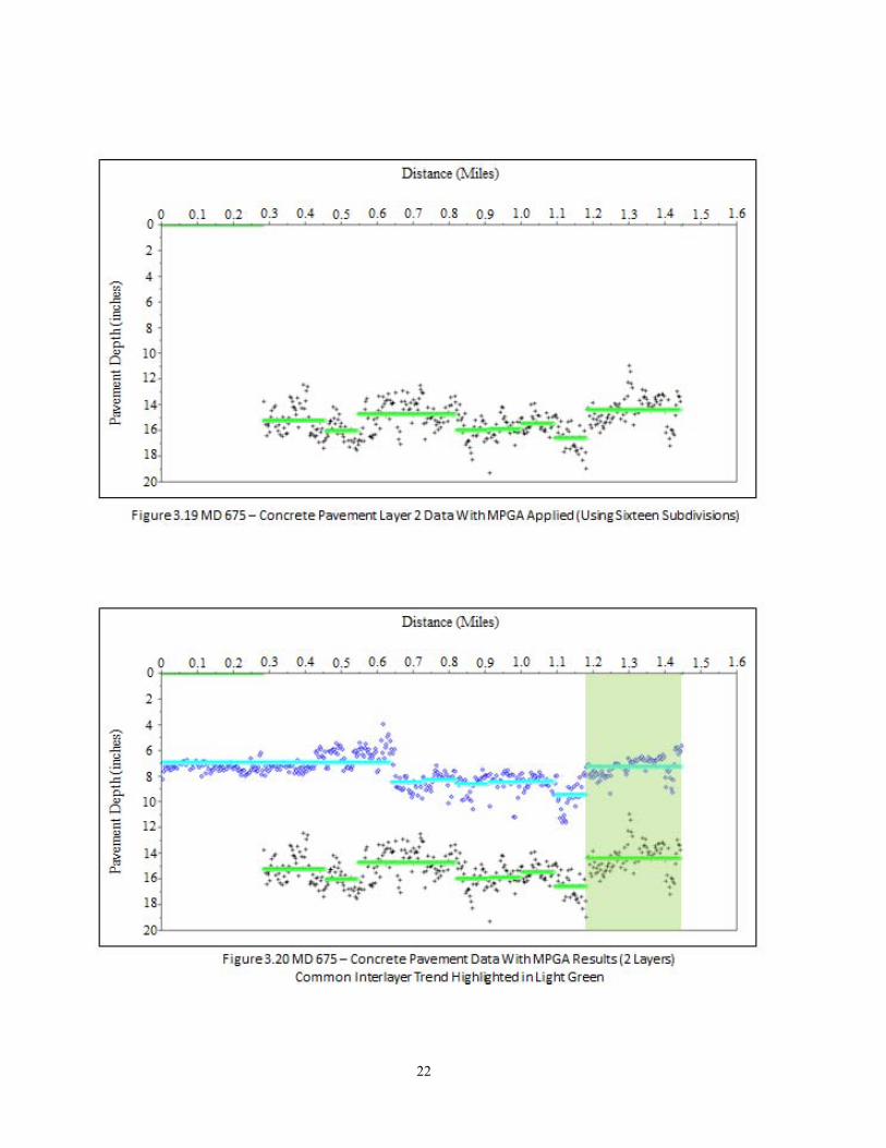
Figures 3.14 through 3.20 provide MPGA results for a section of MD 675 concrete pavement thickness data. The length of this data section is about 1.5 miles, which is significantly shorter than the 11 mile section of US 15 analyzed in Figures 3.1 through 3.13. Figure 3.14 illustrates the final output from the MPGA algorithm for this pavement section, while subsequent figures illustrate how these results were obtained. Figure 3.14 provides MPGA results and thickness data for a two layer concrete pavement. The near surface layer (Layer 1) indicates two segments of consistent thickness (mile 0 to mile 0.65 and mile 1.15 to 1.45) while segments with deeper Layer 1 thickness (mile 0.65 to 1.15) indicate greater thickness variability. MPGA results (shown in aqua for Layer 1) indicate relatively consistent thickness segments. A continuous line while a broken line indicates shorter localized data trends. Similarly, deeper base layer pavement data results are shown in green (corresponding to Layer 2). Layer 2 information was not detected between 0 and 0.25 miles. Also, there are more discontinuities in Layer 2 results than in Layer 1 results. Even so, two continuous segment trends were identified in Layer 2 (mile 0.5 to 0.8 and mile and mile 1.15 to 1.45). An interlayer relationship trend corresponding to one of these continuous Layer 2 segments was identified and discussed later in this summary of results.

12
MPGA criteria and length scales of interest were initially selected by a user. Subsequently, analysis results were produced by the algorithm without further user intervention. Identical user selected MPGA criteria were used on both the US 15 pavement and the MD 675 pavement. Different analysis length scales were selected for each pavement to identify relevant data trends. Figure 3.15 illustrates how mean layer thickness values corresponding to the entire MD 675 data analysis section of interest do not capture thickness variability, while global mean trends pass through local discontinuities but fail to accurately represent continuous thickness segments (where data in these segments appear consistently above or below the global mean trend). Figure 3.16 illustrates how MPGA initially subdivides the MD 675 Layer 1 data section into equal size segments. Subsequently, neighboring local segments with statistical qualities in common are joined together by MPGA, while those that exhibit greater variability in these qualities remain separated, as shown in Figure 17. In a similar manner, subdivision of data into local segments and the subsequent process of joining segments with statistical qualities in common is shown in Figures 3.18 and 3.19 respectively for MD 675 Layer 2 data. Finally, interlayer trends in MPGA results were examined with respect to significant data segment continuity and discontinuity in Figure 3.20, similar to the Figure 3.13 plot for the US 15 data set. Segments that exhibit interlayer continuity characteristics were highlighted in light green in Figure 3.20 (between mile 1.15 and 1.45). A matching discontinuity appears in both Layer 1 and Layer 2 data immediately before this continuous segment (~mile 1.05 to 1.15). Other interlayer trends in the data can quickly be assessed to have less in common than these highlighted segments based on MPGA. These initial analysis results indicate that MPGA has the potential to improve accuracy in pavement thickness data that are used in pavement management and rehabilitation analysis. The MPGA results presented herein indicate that pavement thickness data trends can be identified based on either automated or semi-automated procedures using target variability levels of thickness uniformity, and thus can be used to efficiently evaluate pavement material layers. The MPGA approach is able to effectively identify variable and thin pavement thickness subsections, construction pavement thickness discontinuities, and trends among multiple pavement layers which may indicate possible damage, deterioration, or defects.

13

14
-

15

16

17

18

19

20

21
22

23
CHAPTER 4: GPR BRIDGE DECK ANALYSIS Accurate, efficient bridge deck inspection and evaluation is an important aspect of maintaining valuable MD SHA bridge infrastructure assets. Bridge decks usually wear out much faster than other bridge components, motivating a focus on this aspect of bridge inspection. Key problems with the state of practice bridge inspection have been identified in previous studies including bridge rating accuracy and reliability concerns using conventional techniques. Also, bridge inspections and evaluations are required by U.S. Federal rules to address practical needs to identify bridge safety and maintenance issues quickly and cost effectively. Specific reliability problems with qualitative bridge inspection and evaluation practices using existing visual inspection and complementary techniques such as chain drag sounding further motivate development and implementation of new and emerging alternatives. Therefore, there was a need to investigate how MD SHA can address bridge deck inspection problems more effectively with emerging state of the art solutions. Development and study of bridge deck inspection and evaluation techniques using emerging Ground Penetrating Radar (GPR) technologies is a significant technique to consider due to features such as fast data acquisition speed and quantitative measurement capabilities (described below). This study examined ways to develop and implement more reliable bridge inspection and evaluation using GPR techniques. Currently available GPR data analysis techniques such as migration imaging (for concrete cover depth measurement applications among others), Fourier analysis of GPR waveforms (for qualitative bridge deck moisture analysis) and emerging techniques such as Short Time Fourier Transform analysis (for anticipated quantitative moisture analysis) can be used. Migration and Fourier techniques are illustrated corresponding to GPR data collected using a GPR array on selected bridge decks in the Salisbury, MD area. Figures 4.1 through 4.9 illustrate GPR migration analysis results from a US 13 north bound bridge over a Norfolk Southern railroad track. Migration results are presented as a series of plan view images at 1 inch depth intervals (corresponding to the upper image in each figure). In the migration images, dark colors represent low magnitude responses (low or no GPR reflection) and light colors represent high magnitude responses (strong GPR reflection). The lower image in each of the Figures corresponds to an amplitude/attenuation map of waveform reflections from the top layer of reinforcing steel in the deck (identical in all nine figures). An important observation in Figure 4.3 is the GPR migration image corresponding to a 2 inch depth. This image indicates shallow cover depth reinforcing steel in a few key locations (circled in blue). These locations correlate well with several areas in the Figure 4.3 GPR amplitude/attenuation map (where high amplitude responses indicated in red and yellow are associated with a high probability of deterioration). This correlation is consistent with an increased probability of corrosion deterioration in shallow concrete cover depth areas due to fast diffusion of salts and moisture down to the steel depth. The opposite phenomenon is observed where slower diffusion to deeper steel depths typically results in slower corrosion processes corresponding to areas with greater concrete cover depth. Figure 4.4 indicates the remaining migrated reinforcing steel response features around a cover depth of 3 inches. Subsequent Figures 4.5 through 4.9 illustrate responses at increasing depths down to the underside of the bridge deck.

24
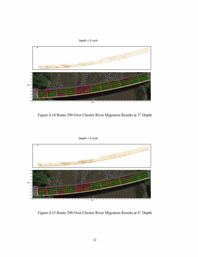
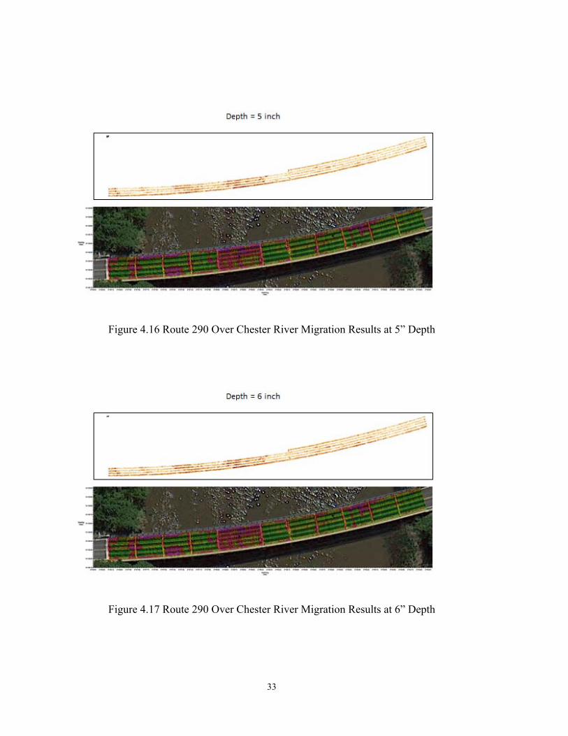
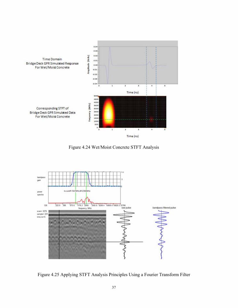
In addition, the top Figure 4.10 image shows a relative moisture map of the US 13 north bound bridge deck over Norfolk Southern Railroad. This relative moisture map was generated by a Fourier analysis of attenuation of migrated GPR response magnitudes through the bridge deck thickness (where the method that produced the top Figure 4.10 image is described later in this section). Probable high moisture content areas are indicated in dark blue while probable low moisture content areas are indicated in aqua. In this Figure 4.10 moisture analysis image, high moisture content areas generally correlate with probable deterioration areas in the corresponding amplitude/attenuation map below it. Figures 4.11 through 4.19 are migration results from an analysis of GPR data collected on a Route 290 bridge crossing the Chester River. Like prior results, these Figures are presented as plan view images of GPR migration outputs at 1 inch depth intervals (from the surface to an 8 inch depth). For this example case, a very shallow cover depth area appears in Figure 4.12, corresponding to a 1 inch depth and circled in blue. This shallow cover depth area generally coincides with the location of the largest probable deterioration area in the corresponding amplitude/attenuation map in Figure 4.12. This feature further reinforces the hypothesis that shallow reinforcing steel often leads to premature corrosion and subsequent bridge deck deterioration. In addition, a few anomalies in Figure 4.16 through 4.19 depth images correlate well with deterioration areas in the amplitude/attenuation map. Finally, the Figure 4.20 map of relative moisture generally indicates higher moisture content in areas where deterioration is most prevalent. A summary of the motivation and theoretical support for a Short Time Fourier Transform (STFT) analysis to quantitatively evaluate bridge deck moisture is presented next in Figures 4.21 through 4.24. This is followed by a practical application of a related Fourier analysis to qualitatively evaluate bridge deck moisture in Figures 4.25 through 4.29. Upon further development, the quantitative STFT approach is anticipated to provide a rapid means to evaluate absolute bridge deck moisture content which can account for the significant effects of moisture on GPR responses (which currently present some important challenges to GPR data interpretation and analysis). The related Fourier analysis presented offers a rapid technique to obtain qualitative (relative) moisture information about bridge decks, which can already improve GPR data analysis and interpretation in a few significant ways. Figure 4.21 shows a ray path diagram corresponding to two theoretical GPR response models, a dry concrete bridge deck and a moist concrete bridge deck. Complex dielectric properties associated with each model are provided and the basic ray path diagrams corresponding to response features of interest (top surface and bottom surface) are shown. Figure 4.22 illustrates how time domain responses to the bridge deck top surface and bottom surface appear in an analytical waveform simulation of moist versus dry concrete. Figure 4.22 shows that the back surface reflection of the moist deck is delayed versus the dry deck and that moisture related dispersion reduces bottom surface GPR response signal energy versus a dry deck. Figures 4.23 and 4.24 show two dimensional STFT responses corresponding to the dry and moist cases respectively. The dominant phenomena revealed by the STFT analysis plot (a frequency versus time representation of the amplitude versus time information) are reduced high frequency content and reduced signal amplitudes (both caused by moisture dispersion phenomena). A time delay associated with the moisture is also observed. In the future an STFT analysis can be developed to quantitatively evaluate bridge deck moisture content based on these response phenomena. Currently, a qualitative Fourier transform analysis of relative moisture content can be performed using related principles and is presented in Figures 4.25 through 4.29.

25
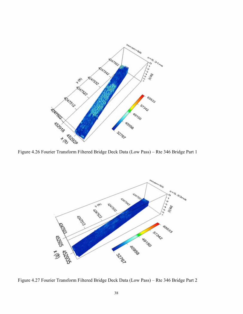
Figure 4.25 presents an example radargram image (position versus time) in the lower left where a vertical line corresponds to the location of a raw waveform pulse shown to its right. A band pass filtered waveform pulse is shown at the far right, which primarily removes high frequency noise and multi-path scattering phenomena from small features (leaving low frequency response features from larger scale features such as the bridge deck surface and back surface). Example GPR waveform frequency content is shown in red above along with the band pass gain filter profile in blue. The filter profile emphasizes frequencies between 1 GHz and 2.3 GHz, which are the lower frequencies of interest for the relative moisture analysis. Figures 4.26 through 4.29 provide Fourier analysis plots corresponding to response features at the depth of the bridge deck bottom surface. In these plots, darker blue areas represent areas with more moisture while aqua and other bright colors represent low moisture areas. Multiple views of the results are shown in Figures 4.26 through 4.29. In Figure 4.29 higher moisture content areas are observed to correlate well with many probable deterioration areas in the corresponding amplitude/attenuation plot. Improved information about these moisture phenomena can be used to enhance the interpretation of GPR data, as shown. Additional moisture plots that used the same analysis for other bridge deck examples were already shown in Figures 4.10 and 4.20. Further development of quantitative STFT moisture analysis can make GPR results even more reliable and effective.
Figure 4.1 US 13 Northbound Over Norfolk Southern RR Migration Results (Above) vs. Attenuation Map (Below)

26
Figure 4.3 US 13 Northbound Over Norfolk Southern RR at 2” Depth
Figure 4.2 US 13 Northbound Over Norfolk Southern RR at 1” Depth

27
Figure 4.4 US 13 Northbound Over Norfolk Southern RR at 3” Depth
Figure 4.5 US 13 Northbound Over Norfolk Southern RR at 4” Depth

28
Figure 4.6 US 13 Northbound Over Norfolk Southern RR at 5” Depth
Figure 4.7 US 13 Northbound Over Norfolk Southern RR at 6” Depth

29
Figure 4.8 US 13 Northbound Over Norfolk Southern RR at 7” Depth
Figure 4.9 US 13 Northbound Over Norfolk Southern RR at 8” Depth

30
Figure 4.10 US 13 Northbound Over Norfolk Southern RR - Moisture
Figure 4.11 Route 290 Over Chester River Migration Results (Above) vs. Attenuation Map (Below)

31
Figure 4.12 Route 290 Over Chester River Migration Results at 1” Depth
Figure 4.13 Route 290 Over Chester River Migration Results at 2” Depth
32
Figure 4.14 Route 290 Over Chester River Migration Results at 3” Depth
Figure 4.15 Route 290 Over Chester River Migration Results at 4” Depth
33
Figure 4.16 Route 290 Over Chester River Migration Results at 5” Depth
Figure 4.17 Route 290 Over Chester River Migration Results at 6” Depth

34
Figure 4.18 Route 290 Over Chester River Migration Results at 7” Depth
Figure 4.19 Route 290 Over Chester River Migration Results at 8” Depth

35
Figure 4.20 Route 290 Over Chester River Migration Results - Moisture
Figure 4.21 Short Time Fourier Transform (STFT) Analysis of Bridge Deck GPR Data

36
Figure 4.22 Time Domain Bridge Deck GPR Data Comparison
(Analytical Waveform Simulation of GPR Response to Wet vs. Dry Concrete)
Figure 4.23 Dry Concrete STFT Analysis
37
Figure 4.24 Wet/Moist Concrete STFT Analysis
Figure 4.25 Applying STFT Analysis Principles Using a Fourier Transform Filter
38
Figure 4.26 Fourier Transform Filtered Bridge Deck Data (Low Pass) – Rte 346 Bridge Part 1
Figure 4.27 Fourier Transform Filtered Bridge Deck Data (Low Pass) – Rte 346 Bridge Part 2

39
Figure 4.28 Plan View Results
Figure 4.29 US 13 SB over MD 346 SB FT Filtered Results (Upper) vs. Attenuation Map (Lower)

40
CHAPTER 5: GPR PRECAST CONCRETE ANALYSIS MD SHA uses precast concrete elements to produce many diverse civil infrastructure components in increasing quantities each year. Using precast concrete elements can be responsive to MD SHA goals to reduce civil infrastructure construction costs, increase construction efficiency, and facilitate quality control improvements versus conventional on site concrete casting. Among these potential benefits, effective implementation of precast concrete element quality control has lagged behind the others for MD SHA applications. Unfortunately, diverse precast concrete element defects and problems have the potential to undermine precast efficiency and cost advantages if they are not addressed. Therefore, precast quality control can benefit from increased MD SHA attention and new tools and methods to address it. Precast quality control (QC) is currently done using labor intensive, reactive performance audits and sporadic inspections with the potential to miss important problems. In fact, these audits and inspections have not been shown to be effective unless many violations of MD SHA protocols and specifications occur frequently at a given precast facility. Quality control of precast concrete elements should be improved consistent with cost and function benefits of precast concrete elements. If not, benefits of construction using precast concrete elements are at risk due to potential performance issues of undetected defects and issues. Precast concrete element quality control may lag other benefits due to a lack of information about systematic quality control tools and resources such as Ground Penetrating Radar (GPR). GPR and complementary tools have potential to address quality control issues rapidly and proactively by detecting relevant defects and issues. Without reliable quality control, MD SHA precast concrete elements are susceptible to:
1. Inadequate concrete cover depth to protect reinforcing steel from premature corrosion. 2. Missing or substandard steel reinforcement components to meet MD SHA strength and
durability requirements. 3. Material thickness that may not meet MD SHA design specifications (too thin and weak or
too thick and heavy). 4. Physical or material issues that do not meet MD SHA specifications.
Using appropriate tools and resources including GPR, precast concrete element testing and evaluation has potential to detect problems before they leave the plant. This can minimize the risk of precast defect or material issues. Appropriate test plans and statistical sampling are also important to achieving desired results. This study included an initial assessment in detecting precast concrete defects using GPR with scans carried out at a precast plant MD SHA sources from. Introductory aspects of GPR imaging relevant to precast concrete component evaluation are illustrated by example three dimensional data (Figures 5.1 through 5.4). Example two dimensional results are shown in Figures 5.5 through 5.18. Diverse precast concrete specimen geometries were evaluated including a wall panel, a header wall, a cylinder, a manhole, a fresh concrete cylinder, and a sound wall. Figures 5.1 through 5.4 present a series of four plan view GPR depth slice images of a reinforcing steel grid, increasing in depth from 1 to 4 inches in each successive image. Each of the four figures
41
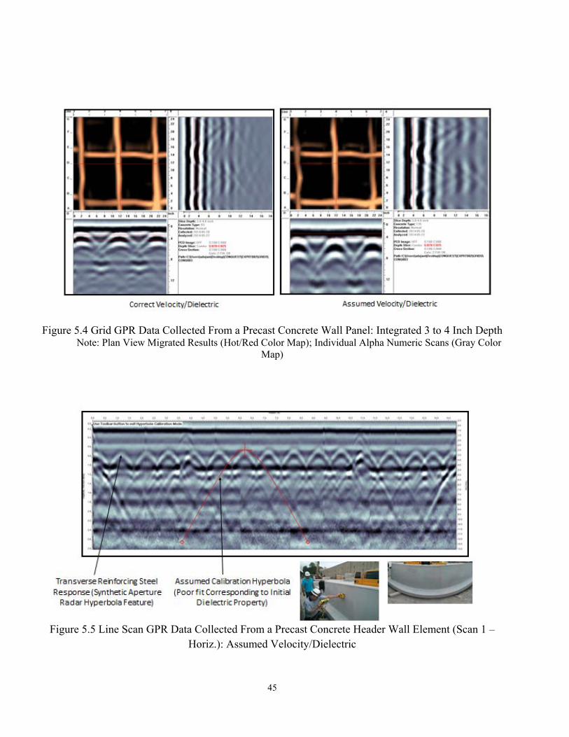
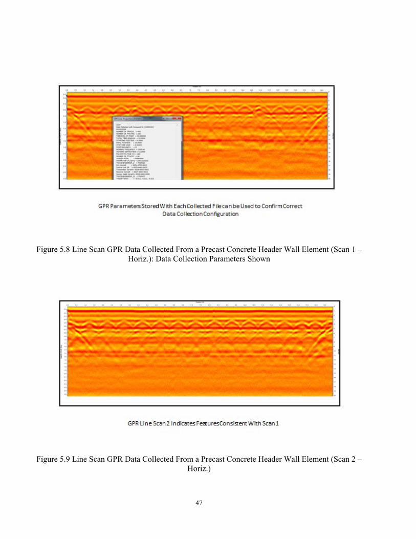
includes a side by side comparison between results corresponding to correct dielectric material properties (at left) and assumed/estimated dielectric material properties (at right). This analysis indicates that correct dielectric material properties allow correct GPR depth measurement results to be determined, but further details about features in the images and details of the analysis are explained later. First, a brief summary of principles used to collect and represent each Synthetic Aperture Radar (SAR) image are reviewed immediately below. In the Figure 5.1 through 5.4 examples, SAR images were built up from a series of GPR antenna scans. During each GPR scan, an antenna consisting of a single transmitter and receiver pair (bistatic) was manually moved along a straight, linear path (following a fixed, marked line). As the GPR antenna moved forward, a GPR encoder wheel turned in proportion to the distance traveled and triggered collection of a GPR waveform approximately three times per inch. Each time of flight GPR waveform measurement includes a series of reflections returned from features with dielectric contrast at increasing depth in the path of the incident GPR wave transmitted by the GPR antenna at a given location. Strong response features in each waveform often correspond to features directly below the antenna pair. However, the incident wave propagates with an approximately cone shaped energy distribution and therefore reflections from some subsurface features adjacent to GPR waveform data collection locations appear in raw GPR waveforms as well. A series of collected waveforms are stacked adjacent to one another to form a SAR image (gray color map images in Figures 5.1 through 5.4). A SAR image collected on a path orthogonal to the detected reinforcing steel appears as a hyperbola shape (as shown in the lower left gray color map images in Figures 5.1 through 5.4). This distributed hyperbola reflection can be focused back to its original reflection source using a technique called migration imaging (reducing the hyperbola shape to the point like shape corresponding to the original reflector). Seven SAR GPR scans were collected in two orthogonal directions and migrated (focused) in three dimensions to produce the focused image of a reinforcing steel grid at upper left in Figures 5.1 through 5.4 (allowing cover depth to be evaluated). Precise alignment of all fourteen GPR scans was maintained by scanning the GPR antenna along a 2 foot square grid template fixed in position on the wall. Various grid template sizes and shapes are available. For migration imaging, the dielectric properties (and corresponding propagation velocity) of the concrete material are accounted for to produce a focused result. One approach involves fitting a hyperbola to a point feature in an SAR image as shown in Figures 5.5 and 5.6. The correct propagation velocity corresponds to the fitted hyperbola shape that matches the reinforcing steel response imaged (for an SAR path orthogonal to the steel orientation). Using the correctly calibrated velocity and dielectric properties results in a correct mapping of depth information to GPR time of flight measurements (as shown in Figure 6 for the header wall pictured in Figure 5). Figure 5.7 presents Figure 5.6 GPR results using an alternative color map (a hot/red Figure 7 color map versus a Figure 5.6 gray color map) illustrating how GPR results can be customized while representing the same underlying information. Figure 5.8 adds a data collection properties window, which specifies parameters such as how many waveform traces make up the SAR image (445 traces) and how far apart each waveform trace sample interval is (0.033 ft). In addition, the center frequency of 1000 MHz is indicated, corresponding to a practical compromise between medium to high resolution and relatively deep penetration capabilities. A parallel scan of the same header wall

42
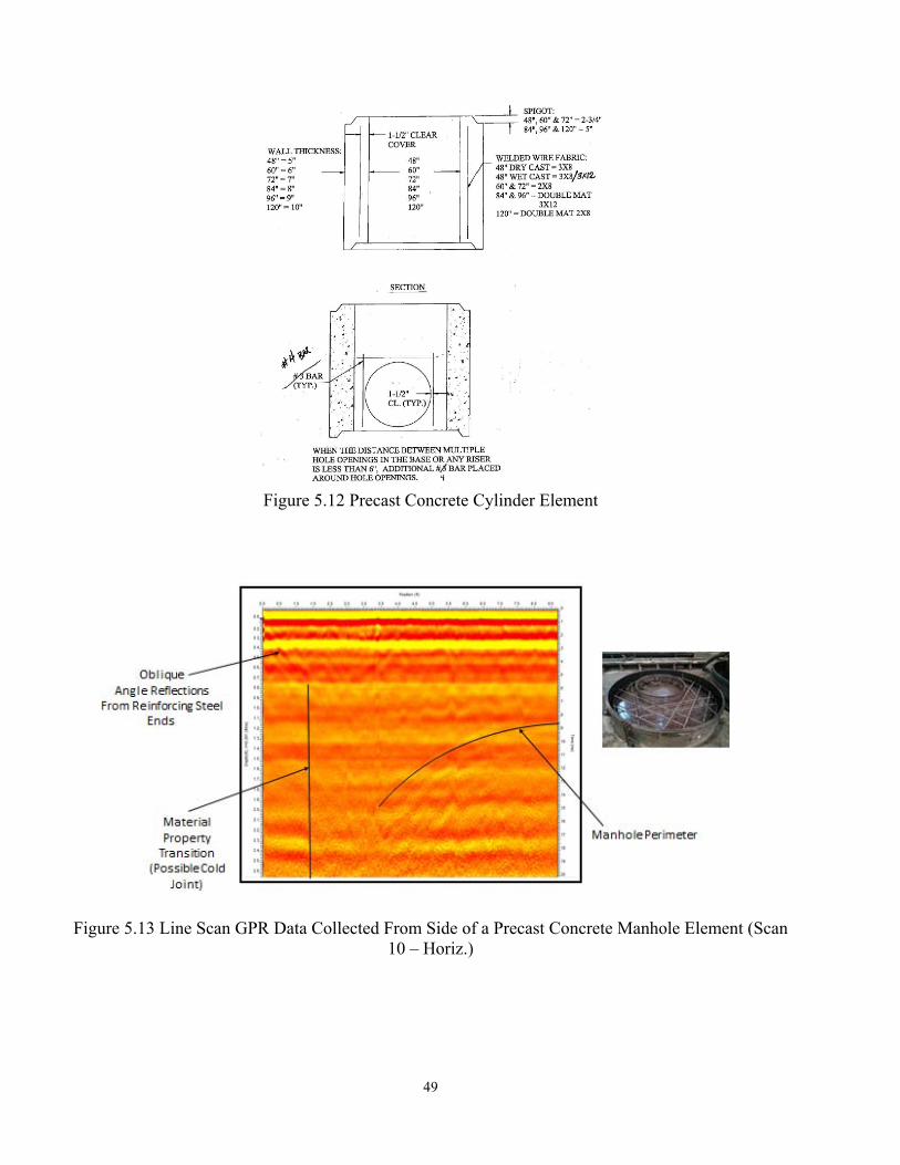
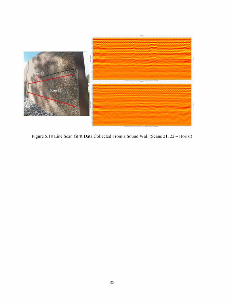
associated with Figures 5.5 through 5.8 is shown in Figure 5.9. The Figure 5.9 scan has the same transverse reinforcing steel spacing as Figure 5.8, indicating vertically oriented reinforcing steel are aligned parallel to each other. Figure 5.10 shows the same header wall reinforcing steel information collected in an orthogonal direction relative to Figure 5.8 and 5.9 scans. Near identical hyperbola features and back wall features between the two scans indicate the precast concrete element was built consistently in the horizontal direction as well. A precast concrete cylinder can present challenges to practical GPR evaluation versus a flat wall due to curved surfaces. However, some GPR system features can make collecting GPR scan data from these cylinder elements more straightforward and reliable. One of these features is a small antenna head size. A small antenna head size can facilitate consistent contact and orientation between the GPR and the test piece. Another feature is an encoder/trigger wheel centered in the antenna head that can maintain surface contact during small orientation changes while the GPR is scanned tangent to the cylinder surface. An example precast concrete cylinder is pictured in Figure 5.11 (scanned during on-site GPR testing at the precast plant) and a drawing corresponding to this example cylinder is shown as provided by the precast plant (Figure 5.12). The cylinder wall reinforcing steel was imaged using GPR and a back wall depth response is indicated in addition to reinforcing steel hyperbola response features. The small antenna size and the centered GPR trigger wheel position on the antenna scan head provided clear, useful Figure 5.12 data (collected orthogonal to the cylinder axis). In addition, GPR cover depth and wall thickness are accurately represented based on a hyperbola calibration fit. Figure 5.13 shows a GPR response to a concrete manhole element. Example formwork is also pictured in Figure 5.13 and illustrated in a plan provided by the precast plant (shown in Figure 5.14). The GPR results obtained indicate why this type of test piece presents challenges to address quality control needs. The GPR was scanned along the perimeter of the cylindrical manhole slab to evaluate for adequate cover depth (while directed inward toward its center). Ideally, reinforcing steel bar ends in several orientations should be clearly imaged in addition to other complementary features to obtain quality control metrics from. These bars are observable in the data, but further refinement and testing of antenna data collection paths is recommended due to sensitivity to unique reinforcing steel orientations. This refinement could improve imaging effectiveness and contrast for useful GPR evaluation of this complex shape. Never the less, significant features such as a material property transition (possibly moisture related) and the manhole perimeter were detected in the data as shown in Figure 5.13. Another concrete cylinder was evaluated inside the precast plant building to show the effects of fresh concrete material properties on GPR response characteristics (Figure 5.15). Hyperbola fitting confirmed GPR wave velocities were reduced to 0.249 ft/ns in fresh, moist concrete versus a velocity of 0.261 ft/ns in more mature, dry concrete (Figure 5.11). Significant GPR signal energy losses were also observed in reinforcing steel responses when Figure 5.11 (dry concrete) and Figure 5.15 (moist concrete) images were compared. It is evident that this was due to GPR energy losses that occur as GPR waves pass through moist material. A vertical scan of the same moist, fresh concrete cylinder in Figure 16 exhibits similar imaging characteristics observed in Figure 5.15, but the thin gage wire mesh produces a diffraction effect rather than a hyperbola response due to its mall diameter. Finally, a sound wall in the field is shown in Figures 5.17 and 5.18. A vertical GPR wall scan is shown in Figure 5.17 and two horizontal scans of the wall are shown in Figure 5.18. Even though the

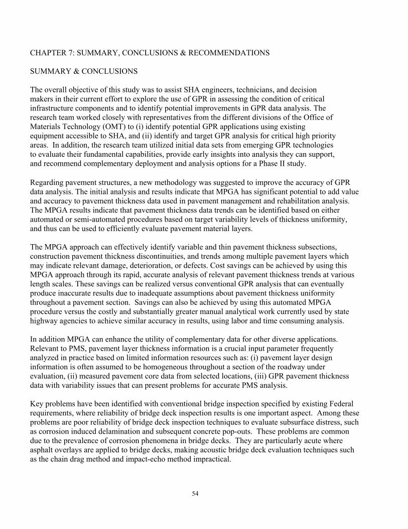
43
surface of the wall was uneven, steel reinforcement depth and orientation were consistently detected by the GPR in both scan orientations. The reinforcement appears to be thin wire rather than steel bars based on the close spacing and diffraction response observed. Refinement of sampling and test methodology is recommended. Hand held GPR techniques were tested and demonstrated for applications to precast concrete elements on-site at a precast concrete plant MD SHA sources from. Key GPR system features that enabled effective, practical testing were highlighted. The testing and demonstration showed significant potential for quality control using GPR parameter measurement such as concrete cover depth and geometry, concrete moisture content, and more. Further testing and refinement of GPR techniques for evaluation of specific defects is recommended to design more complete data collection scan patterns, hardware settings, and to refine post processing analysis.
Figure 5.1 Grid GPR Data Collected From a Precast Concrete Wall Panel: Integrated 0 to 1 Inch Depth
Note: Plan View Migrated Results (Hot/Red Color Map); Individual Alpha Numeric Scans (Gray Color Map)

44
Figure 5.2 Grid GPR Data Collected From a Precast Concrete Wall Panel: Integrated 1 to 2 Inch Depth
Note: Plan View Migrated Results (Hot/Red Color Map); Individual Alpha Numeric Scans (Gray Color Map)
Figure 5.3 Grid GPR Data Collected From a Precast Concrete Wall Panel: Integrated 2 to 3 Inch Depth Note: Plan View Migrated Results (Hot/Red Color Map); Individual Alpha Numeric Scans (Gray Color
Map)
45
Figure 5.4 Grid GPR Data Collected From a Precast Concrete Wall Panel: Integrated 3 to 4 Inch Depth Note: Plan View Migrated Results (Hot/Red Color Map); Individual Alpha Numeric Scans (Gray Color
Map)
Figure 5.5 Line Scan GPR Data Collected From a Precast Concrete Header Wall Element (Scan 1 –
Horiz.): Assumed Velocity/Dielectric

46
Figure 5.6 Line Scan GPR Data Collected From a Precast Concrete Header Wall Element (Scan 1 - Horiz): Correct Velocity/Dielectric
Figure 5.7 Line Scan GPR Data Collected From a Precast Concrete Header Wall Element (Scan 1 – Horiz.): Correct Velocity/Dielectric (Hot/Red Color Map)
47
Figure 5.8 Line Scan GPR Data Collected From a Precast Concrete Header Wall Element (Scan 1 – Horiz.): Data Collection Parameters Shown
Figure 5.9 Line Scan GPR Data Collected From a Precast Concrete Header Wall Element (Scan 2 –
Horiz.)

48
Figure 5.10 Line Scan GPR Data Collected From a Precast Concrete Header Wall Element (Scans 3
and 4 – Vert.)
Figure 5.11 Line Scan GPR Data Collected From a Precast Concrete Cylinder Element (Scan 5 –
Horiz.)
49
Figure 5.12 Precast Concrete Cylinder Element
Figure 5.13 Line Scan GPR Data Collected From Side of a Precast Concrete Manhole Element (Scan
10 – Horiz.)

50
Figure 5.14 Precast Concrete Manhole Element
Figure 5.15 Line Scan GPR Data Collected From a Moist Precast Concrete Cylinder Element (Scan 11
– Horiz.)

51
Figure 5.16 Line Scan GPR Data Collected From a Moist Precast Concrete Cylinder Element (Scan 17
– Vert.)
Figure 5.17 Line Scan GPR Data Collected From a Sound Wall (Scan 20 – Vert.)
52
Figure 5.18 Line Scan GPR Data Collected From a Sound Wall (Scans 21, 22 – Horiz.)

53
CHAPTER 6: GPR TESTING PROTOCOLS AND TRAINING MODULES The research team developed the testing protocols for GPR evaluation of pavement structures and bridge decks. The testing protocols follow the SHA structure for MSMTs and include sections describing the following:
• Scope;
• Reference Documents;
• Terminology;
• Summary Method (background);
• Apparatus;
• Periodic Calibration;
• Testing Procedure & Data Collection;
• Routine Calibration;
• Data Analysis;
• Reporting;
The protocols are included in the Appendix A. The research team also developed training modules for the assessment of pavement structures, bridge decks and precast concrete elements. These modules are included in Appendix B and include information related to:
• Summary Method (background);
• Apparatus Characteristics & Applicable Calibrations;
• Examples of Data Analysis.
54
CHAPTER 7: SUMMARY, CONCLUSIONS & RECOMMENDATIONS SUMMARY & CONCLUSIONS The overall objective of this study was to assist SHA engineers, technicians, and decision makers in their current effort to explore the use of GPR in assessing the condition of critical infrastructure components and to identify potential improvements in GPR data analysis. The research team worked closely with representatives from the different divisions of the Office of Materials Technology (OMT) to (i) identify potential GPR applications using existing equipment accessible to SHA, and (ii) identify and target GPR analysis for critical high priority areas. In addition, the research team utilized initial data sets from emerging GPR technologies to evaluate their fundamental capabilities, provide early insights into analysis they can support, and recommend complementary deployment and analysis options for a Phase II study. Regarding pavement structures, a new methodology was suggested to improve the accuracy of GPR data analysis. The initial analysis and results indicate that MPGA has significant potential to add value and accuracy to pavement thickness data used in pavement management and rehabilitation analysis. The MPGA results indicate that pavement thickness data trends can be identified based on either automated or semi-automated procedures based on target variability levels of thickness uniformity, and thus can be used to efficiently evaluate pavement material layers. The MPGA approach can effectively identify variable and thin pavement thickness subsections, construction pavement thickness discontinuities, and trends among multiple pavement layers which may indicate relevant damage, deterioration, or defects. Cost savings can be achieved by using this MPGA approach through its rapid, accurate analysis of relevant pavement thickness trends at various length scales. These savings can be realized versus conventional GPR analysis that can eventually produce inaccurate results due to inadequate assumptions about pavement thickness uniformity throughout a pavement section. Savings can also be achieved by using this automated MPGA procedure versus the costly and substantially greater manual analytical work currently used by state highway agencies to achieve similar accuracy in results, using labor and time consuming analysis. In addition MPGA can enhance the utility of complementary data for other diverse applications. Relevant to PMS, pavement layer thickness information is a crucial input parameter frequently analyzed in practice based on limited information resources such as: (i) pavement layer design information is often assumed to be homogeneous throughout a section of the roadway under evaluation, (ii) measured pavement core data from selected locations, (iii) GPR pavement thickness data with variability issues that can present problems for accurate PMS analysis. Key problems have been identified with conventional bridge inspection specified by existing Federal requirements, where reliability of bridge deck inspection results is one important aspect. Among these problems are poor reliability of bridge deck inspection techniques to evaluate subsurface distress, such as corrosion induced delamination and subsequent concrete pop-outs. These problems are common due to the prevalence of corrosion phenomena in bridge decks. They are particularly acute where asphalt overlays are applied to bridge decks, making acoustic bridge deck evaluation techniques such as the chain drag method and impact-echo method impractical.

55
GPR data collection speed, coverage, and material penetration for practical concrete bridge deck applications, has improved steadily over the years due to features such as synchronized antenna arrays (for rapid, parallel path data collection using several antenna elements together) and improved instrument signal to noise ratios (within practical and regulatory limits). These GPR hardware advances have made many potential bridge deck evaluation advances possible, but relatively few GPR systems have been applied broadly in practice by agencies such as MD SHA to the present. In part, this may be due to recognition of needs to improve analysis of GPR data to extract valuable, potentially reliable information (such as locations and quantities of bridge deck deterioration phenomena to scope repair, rehabilitation, or replacement decisions). In addition, there is a need to control for variables such as concrete moisture content, which can impact existing bridge deck GPR results significantly in some scenarios. Thus, in this study, currently available GPR data analysis techniques such as migration imaging (for concrete cover depth measurement applications among others) and Fourier analysis of GPR waveforms (for qualitative bridge deck moisture analysis) in addition to emerging techniques such as Short Time Fourier Transform analysis (for anticipated quantitative moisture analysis) were applied in novel ways. Migration and Fourier techniques were illustrated corresponding to GPR data collected using a GPR array on selected bridge decks in the Salisbury, MD area. When applied appropriately, such techniques can provide more reliable analysis of bridge deck inspection then conventional means. Currently precast concrete QC is based on plant inspections and periodic audits. These quality assurance practices include labor intensive activities and sporadic inspections with the potential to miss important problems. In fact, these audits and inspections have not been shown to be effective unless many violations of MD SHA protocols and specifications occur frequently at a given precast facility. This study has shown how GPR can be used to address several of the inspections needed in precast concrete production, including an evaluation of concrete cover depth, reinforcement location, and section thicknesses. The testing and demonstration showed significant potential for quality control using GPR. Further testing and refinement of GPR techniques for evaluation of specific defects is recommended to design more complete data collection scan patterns, hardware settings, and to refine post processing analysis. For the high priority areas of pavement structures and bridge decks the project team developed the required testing protocols, in MSMT format, to facilitate the implementation of GPR and assist SHA engineers and technicians to conduct such surveys. The protocols include among other information related to the method (background), equipment requirements, calibration guidelines, testing procedure and recommendations for data analysis and reporting. Along with the testing protocols the research team developed training material for pavement structures, bridge decks and precast concrete elements. In parallel to this project SHA contracted the use of emerging GPR technologies in bridge decks including an efficient ground coupled impulse GPR antenna array system and a high speed, step frequency GPR array system with many configuration options for advanced applications. Initial pilot analysis by the project team included (i) bridge deck deterioration evaluation (where relative moisture content was estimated as a contributing factor), and (ii) quality control/quality assurance parameters (including concrete cover depth) to predict probable deterioration areas. Both technologies provided promising initial information for this study, but high speed (30+ mph) step frequency GPR capabilities and wider coverage area per data collection pass (in addition to potential refinement of versatile

56
materials evaluation and geometry measurements) were recognized by SHA as high priorities for future work. Therefore, techniques to quantitatively evaluate deterioration factors such as moisture content and active bridge deck corrosion will be developed to leverage step frequency GPR in a Phase II study of bridge decks (at project and network levels) and pavements (at the project level). In addition, step frequency GPR technology can be used to advance MPGA analysis for improved ease of use and further refinement of the analysis. The expected benefits of the proposed GPR based condition assessment techniques include: i) higher precision and accuracy of the condition assessment of key infrastructure components and materials; ii) higher speed of condition assessment reducing monitoring time and cost; iii) increasing accuracy of the specific locations where failures occur; iv) improving overall condition assessment methods and more accurate performance and life cycle predictions; v) facilitating a method of non-destructive testing for Quality Assurance testing and forensic investigations.
RECOMMENDATIONS FOR FUTURE DEVELOPMENT
The results of this study provide the following recommendations in order to improve and successfully implement GPR surveys within SHA:
Further refine the post processing analysis techniques for pavement structures for their adoption in the routine GPR analysis by SHA;
Develop analysis techniques to capture moisture effects more precisely in bridge deck GPR analysis, and better relate moisture with deterioration;
Develop GPR based deterioration criteria for project level (i.e., density/ location of distress) and network level (i.e., overall condition ranking) analysis of pavement structures and bridge decks;
Custom tailor testing techniques for different configuration/ shape of precast concrete elements in order to improve accuracy of GPR analysis;
Develop NDE/GPR based criteria for QA/QC procedures and acceptance of pavements, bridge decks and precast concrete elements;
Augment existing SHA GPR equipment to expand capabilities and pilot test a universal system for multiple applications;
Enhance in-house SHA GPR expertise by identifying GPR team leaders within each division and establishing a GPR focus group within OMT.

57
REFERENCES Al-Qadi, I.L., Lahouar, S., Loulizi, A., “Successful Application of GPR for Quality Assurance/Quality
Control of New Pavements,” Paper No. 03-3512, Proceedings of the Transportation Research Board 2003 Annual Meeting, pp. 1-21, 2003.
Al-Qadi, I.L., Lahouar, S., Loulizi, A., “Ground-Penetrating Radar Calibration at the Virginia Smart Road and Signal Analysis to Improve Prediction of Flexible Pavement Layer Thicknesses,” Report No. FHWA/VTRC 05-CR7, January 2005, pp. 1-65.
Al-Qadi, I.L., Lahouar, S., “Part 4: Portland Cement Concrete Pavement: Measuring Rebar Cover Depth in Rigid Pavements With Ground Penetrating Radar,” Transportation Research Record: Journal of the Transportation Research Board, 2005, pp. 81-85.
Bois, K., Benally, A., Zoughi, R., “Near-Field Microwave Reflection Property Analysis of Concrete Using Open-Ended Rectangular Waveguites at S- and X-Band”, Poceedings of SPIE Vol. 3396, Nondestructive Evaluation of Materials and Composites II, No. 37, March 31, 1998, pp. 37-46.
Cabrera R. “ Optimal GPR Antena Selection.” Geoscanners AB , Enviromental Expert Article, May 2012.
Daniels, D.J., Ground Penetrating Radar, 2nd Edition, IEEE, pp. 1-726, 2004. De Souza T., Anna, A., Redman J., Hu, N. “ Monitoring the Ground Penetrating Radar Response of
Curing Concrete.” 16th WCNDT 2004 - World Conference on NDT. Montreal, Canada. Aug 30 - Sep 3, 2004.
Diefenderfer, B.K., Mokarem, D.W., Sharp, S.R., “Use of Nondestructive Evaluation to Detect Moisture in Flexible Pavements,” VTRC Report No. 06-R37., 2006, pp. 1-32.
Evans, R., Optimizing Ground Penetrating Radar (GPR) to Assess Pavements.” Loughborough University, Thesis, U.K. 2009.
FHWA. GPR Measuring Pavement Layer Thickness.” FHWA publication HIF 00015. Office of Asset Management., Washington D.C. 2000.
Finck., F. “ Introduction of GPR System for Investigations on Concrete Structures.” Otto-Graf-Journal Vol. 14, 2003.
Gehrig, M., Morris, D., Bryant J. “Ground Penetrating Radar for Concrete Evaluation Studies.” Foundation Performance Association Meeting, March 2004.
GSSI. “ GSSI Handbook for RADAR Inspection of Concrete.” Geophysical Survey Systems Inc., Salem, New Hampshire. August 2006.
Huston, D., Fuhr, P., Maser, K., Weedon, W., “Nondestructive Testing of Reinforced Concrete Bridges Using Radar Imaging Techniques,” New England Transportation Consortium, NETCR 94-2 Final Report, pp. 1-182, July 1, 2002.
Kim, S., Surek, J., Baker-Jarvis, J., “Electromagnetic Metrology on Concrete and Corrosion,” Journal of Research of the National Institute of Standards and Technology, Vol. 116, No. 3, May-June 2011, pp. 655-669.
Lahouar, S., “Development of Data Analysis Algorithms for Interpretation of GPR Data,” Virginia Polytechnic Institute and State University Thesis, 2003.
Loken., W. “ Use of Ground Penetration Radar to Evaluate Minnesota Roads.” Minnesota DOT. Report MN/RC-2007-01. Saint Paul, MN. 2007
Maser, K., “Use of Ground Penetrating Radar Data for Rehabilitation of Composite Pavements on High-Volume Roads, Transportation Research Record, Vol 1808, 2002, pp. 122-126.
Maser, K., “Ground Penetrating Radar Data for Pavement Evaluation, Annual Road Profiler Users Group: Pavement Evaluation, Roanoke, VA, 2010.

58
Maser, K., Martino, N., Doughty, J., Briken, R., “Understanding and Detecting Bridge Deck Deterioration Using Ground Penetrating Radar,” TRB 91st Annual Meeting, Paper 12-1765, 2012.
Morey R. “ GPR for Evaluating Subsrafce Conditions for Transpoortation Facilities.” Synthesis of Highway Practice 255. TRB, Washington D.C. 1998.
Minnesota DOT, “Pavement Evaluation Using Ground Penetration Radar.” Technical Summary 2008-10TS, Saint Paul, MN. 2008.
Olhoeft, G., Smith S. “Automatic Processing and Modeling of GPR Data for Pavement Thickness and Properties.” Eighth International Conference on Ground Penetrating Radar, Gold Coast, Australia, April 2000.
Pailes, B.M., Gucunski, N., Brown, M., “Correlation of Non-destructive Testing Results to Improve Assessment of Corrosion and Corrosion Damage of a Reinforced Concrete Deck,” Proceedings of the Transportation Research Board 92nd Annual Meeting, Washington, D.C., January 13-17, 2013.
Perkins, A.D., Amrol, J.J., Romero, F.A., Roberts, R.L., “DOT Specification Development Based on Evaluation of Ground-Penetrating Radar System Performance in Measuring Concrete Cover (Reinforcement Depth) on New Bridge Deck Construction,” Structural Materials Technology IV: an NDT Conference, Editor: Sreenivas Alampalli, New York State Dept. of Transportation, March 2000, pp. 53-60.
Scott, M., Rezaizadeh, A., Delahaza, A., Santos, C.G., Moore, M., Graybeal, B., Washer, G., “A Comparison of Nondestructive Evaluation Methods for Bridge Deck Assessment,” Nondestructive Testing and Evaluation International, Vol. 36, 2003, pp. 245-255.
Scott, M., Nondestructive Testing Handbook, Vol. 5, Electromagnetic Testing, Chapter 17, Part 2, Infrastructure Applications of Electromagnetic Testing, American Society for Nondestructive Testing, 2004, pp. 430-436.
Scullion, T., “Implementing Ground Penetrating Radar Technology Within TXDOT,” Texas Department of Transportation, Report No. FHWA/TX-05/5-1702-01-1, March 2005.
SHRP 2, Report S2-R06-RW: “A Plan for Developing High-Speed, Nondestructive Testing Procedures for Both Design Evaluation and Construction Inspection.” TRB, Washington D.C., 2009.
SHRP 2, Report S2-R06A-RR-1: “Nondestructive Testing to Identify Concrete Bridge Deck Deterioration.” TRB, Washington D.C., 2013.
SHRP 2, Report S2-R06C-RR-1: “Using Infrared and High-Speed Ground Penetrating Radar for Uniformity Measurements on New HMA Layers.” TRB, Washington D.C., 2013.
SHRP 2 Renewal Project R06D, “Nondestructive Testing to Identify Delaminations between HMA Layers.” TRB, Washington D.C., 2013.
Smith, S.S., Scullion, T., “Development of Ground-Penetrating Radar Equipment for Detecting Pavement Condition Preventive Maintenance,” Strategic Highway Research Program, Report No. SHRP-H-672, October 1993, pp. 1-178.
Stolt, R., “Migration by Fourier Transform,” Geophysics, Vol. 43, No. 1, February 1978, pp. 23-48. South Dakota DOT. “Feasibility of Using Ground Penetrating Radar (GPR) for Pavements, Utilities,
and Bridges.” Report SD2005-05-X. South Dakota Department of Transportation, Pierre, SD. 2006.

59
Tinkey, Y., Miller, P., Leonard, M., Pott, A., Olson, L., “Bridge Deck Scanning for Condition Assessments of Bare Concrete and Asphalt Overlaid Decks,” Proceedings of the Transportation Research Board 92nd Annual Meeting, Washington, D.C., January 13-17, 2013.
White, J., Wolf, J., Shokouhi, P., Hurlebaus, S., Wimsatt, A., “Concrete Tunnel Lining Evaluation Using Nondestructive Techniques: A Multi-Method Case Study at Eisenhower Tunnel,” Proceedings of the Transportation Research Board 92nd Annual Meeting, Washington, D.C., January 13-17, 2013.
Willett, D., Rister B. “GPR Pavement Layer Thickness Evaluation.” Kentucky Transportation Center, Report KTC 02—29, Lexington, Kentucky. 2002
Zoughi, R., Cone, G.L., Nowak, P.S., “Microwave Non-destructive Detection of Rebars in Concrete Slabs,” Materials Evaluation, Vol. 49, No. 11, November 1991, pp. 1385-1388.

60
APPENDIX A TESTING PROTOCOLS

61
Approval:
Maryland Department of Transportation State Highway Administration Office of Materials Technology
MARYLAND STANDARD METHOD OF TESTS
Approved:
GPR FOR PAVEMENT STRUCTURES
MSMT xxx
SCOPE: This procedure is used to determine the thickness of pavement layers using ground penetration radar. This non‐destructive pavement evaluation method could identify defects in pavement materials and structures, such as material property deterioration, voids, moisture concentration, other. REFERENCE DOCUMENTS: ASTM 4748‐10, “Standard Test Method for Determining the Thickness of Bound Pavement Layers
Using Short‐Pulse Radar.” AASHTO, “Standard Practice for Application of Ground Penetrating Radar (GPR) to Highways,” Report
No. R037‐04‐UL, 2009, pp. 12. Daniels, D.J., Surface Penetrating Radar, The Institution of Electrical Engineers, pp. 320, December
1996. Sebesta, S., Scullion, T., Saarenketo, T., “Using Infrared and High‐Speed Ground‐Penetrating Radar for
Uniformity,” Transportation Research Board (TRB), Strategic Highway Research Program (SHRP2) Renewal Research, Report No. S2‐R06C‐RR‐1, pp. 80, 2013.
Wenzlick, J.D., Scullion, T., Maser, K., “High Accuracy Pavement Thickness Measurement Using Ground Penetrating Radar (Nondestructive Testing for Quality Control of New Pavement),” MoDOT Report No. RDT 99‐003, February 1999, pp. 104.
Zhou, F., Scullion, T., “Guidelines for Evaluation of Existing Pavements for HMA Overlay,” Report FHWA/TX‐07/0‐5123‐2, May 2007, pp. 110.
TERMINOLOGY: Antenna is a transmitting GPR antenna that converts an excitation in the form of a voltage pulse or wave train into EM waves. A receiving GPR antenna converts energy contained in EM waves into voltages, which are regarded as GPR data upon digital sampling of analog voltages, and storage of quantized values. Bistatic Antenna is an antenna configuration that incorporates two antennas, where the first antenna radiates incident EM waves toward the ground and the second antenna receives the reflected waves.
62
Bandwidth is the operating frequency range of an antenna, typically the difference between the upper and lower 3‐dB frequencies (i.e., upper and lower 3 dB frequencies relative to the antenna’s resonant frequency).
Coupling between the GPR antenna and the ground is indicated by the efficiency of the antenna transmitting electromagnetic energy into the ground, where “good” coupling is indicated by efficient transmission of EM energy from the antenna into the ground within the antenna bandwidth and “poor” coupling is indicated by low efficiency transmission of EM energy from the antenna into the ground within the antenna bandwidth.
Depth of Penetration is the maximum depth range a radar signal can penetrate into a given material.
Attenuation is the loss of EM wave energy due to conduction currents.
Scattering is the change in direction of electromagnetic wave propagation that occurs at a change in material properties over a short distance compared to a wavelength for an interval comparable to or greater than a wavelength. Scattering includes reflection (reverse change in direction), refraction (forward change in direction), and diffraction (caused by rapid changes that are small compared to a wavelength in both occurrence and interval).
Time gain is the amplification applied to a trace as a function of time, where the function can be continuous or piecewise depending on data analysis requirements.
Transmit Pulse is the voltage impulse that excites the transmitting antenna.
Polarization (polarization vector) is the orientation of the direction of the vector electromagnetic field. Many GPR antennas are linearly polarized.
Conductivity is the ability of a material to support movement of electrons or ions due to an applied electrical field.
Diffusion is the movement of charges in response to an applied electric fieldor in response to an applied time‐varying magnetic field. Diffusion is the low‐frequency, high‐loss, limiting behavior of electromagnetic wave propagation and is descriptive of behavior that decays rapidly (exponentially) with distance and time.
Dispersion is a material characteristic where wave velocity is no longer uniquely defined, giving rise to the distinction of phase velocity and group velocity. For example, elevated water content in dielectric civil engineering materials (such as concrete and asphalt) results in increased dispersion effects, where electromagnetic waves become increasingly spread out as a function of frequency.
Dielectric Permittivity is the property that describes the ability of a material to store electric energy by separating opposite polarity charges in space. It relates ability of a material to be polarized in response to the application of an electric field.
Relative Permittivity (relative dielectric permittivity; Dielectric Constant) is the ratio of the dielectric permittivity of a material to the permittivity of free space (or vacuum).

63
Magnetic Permeability (μ) is the property that describes the ability of a material to store magnetic energy by realignment of electron spin and motion. It relates ability of a material to be magnetized (magnetic polarization).
SUMMARY OF METHOD (background): This test method provides the means for measuring pavement layer thicknesses of existing, new, or rehabilitated pavements. Furthermore, follow‐up data processing could reveal potential defects and deterioration in pavement materials and structures. As the electromagnetic wave generated by radar propagates through the pavement layers, the wave is attenuated, diffused, and dispersed within material layers and scattered (reflected, refracted, or diffracted) at layer interfaces. The maximum penetration depth depends (among other things): on the ground penetration radar system used (such as transmitted power, receiver sensitivity, center frequency and bandwidth) of the radar system, the electromagnetic properties of the pavement materials; and environmental factors (such as moisture content). The detection of an interface between two different materials depends upon the partial reflection of incident energy at that interface. The amplitude of the reflected energy at that interface, with respect to the incident energy, is related to the relative dielectric constants of the two materials:
(1) where: A = the reflected energy, amplitude A0 = the incident energy, amplitude
1 = the dielectric constant material 1, and
2 = the dielectric constant material 2.
The ability to detect the thickness of a layer depends on the contrast between the dielectric constant of that layer and the layer beneath. Layer thickness can be determined using radar technology if the dielectric constant of that material and the two‐way travel time for the radar wave to pass through the layer are known. The relationship is defined by the following equation:
(2) where: T = layer thickness, c = speed of light in air, 300 mm/nsec for T in mm (11.8 in/nsec for T in inches),
r = relative dielectric constant of layer, and t = two‐way pulse travel time through layer (in nanoseconds). The dielectric constant of a pavement material can vary within a typical range depending on aggregate types, asphalt cement sources, density, cracking, voids, foreign matter, moisture content, and other less common variables. Using an air‐coupled horn antenna radar the real part of this

64
variation may be calculated directly from the radar data by using the known dielectric constant of air and equation (1). Determining the dielectric constant when using ground coupled dipole antenna radar requires an independent means, such as coring, or a radar based dielectric constant measurement. Radar based dielectric constant measurements can be performed using multi‐static antenna pairs positioned at two or more transmitter to receiver location offsets. Using this approach, material properties are subsequently analyzed with techniques such as the Common Midpoint (CMP) method. APPARATUS: The radar system for this application should have a resolution sufficient to determine a minimum layer thickness of 40 mm (1.5 in.) to an accuracy of 6.5 mm (0.25 in.). The apparatus consists of an antenna, radar transducer, and display. The radar transducer consists of a transmitter, receiver, and timing and control electronics. The display device includes a personal computer with a data acquisition board. The transducer generates, transmits, and receives broad band radio frequency (rf) signals through the antenna, that are then converted into an audio frequency signal for display and data interpretation. For HMA applications, an air‐coupled horn antenna of ≥ 1.5 GHz center frequency is used with the manufacturer suggested distance above the pavement surface. Additional antennas of the same frequency or medium (900 MHz) to low (400 MHz) frequency may be incorporated into the radar system in a cross polarized configuration to evaluate pavement cracking phenomena. A medium to low frequency (≤ 1 GHz) ground coupled GPR in a sled configuration may be used is used to provide deep penetration. For concrete pavements medium to low frequency (≤ 1 GHz) ground coupled GPR in a sled configuration is used to provide deep penetration. The transmitter has a short‐pulse (0.5 to 2.0 ns) rate compatible with United States/FCC restrictions. A wide band receiver is used for processing time signals corresponding to a depth of several feet. The data reduction process has the capability to provide pavement thickness within 7% of actual (as measured using reference pavement cores). The GPR system output includes *.kml format files that include geo‐referenced position information. PERIODIC CALIBRATION The following GPR system calibrations should be performed at least once annually.
‐ Time Constant, CT, Calibration: Perform time constant calibration and stability measurement procedures (such as noise‐to‐signal ratio, signal stability, and long‐term signal stability tests) as described in Appendix A.
‐ Signal Calibration: Perform calibration and stability measurement procedures (such as signal‐to‐noise ratio, signal stability, long‐term signal stability tests) as described in Appendix A.
TESTING PROCEDURE & DATA COLLECTION:
‐ Select GPR antenna frequency to penetrate expected depth of pavement structure. A GPR antenna with center frequency of ≥ 2 GHz and wide bandwidth will provide high resolution.

65
‐ Mount GPR antenna at manufacturer specified height and vehicle clearance.
‐ Electronic equipment should be turned on and allowed to warm up and stabilize before any
testing is performed. Refer to manufacturer’s manual for the stabilization period.
‐ Set the GPR configuration to the maximum Pulse Repetition Frequency (PRF) available for the
GPR equipment specified for the application. Select this configuration to maximize the Ground
Penetrating Radar (GPR) response waveform Signal to Noise Ratio (SNR).
‐ Perform routine calibration described next.
‐ For flexible pavement surveys collect GPR data using a GPR system with an air coupled antenna (≥2 GHz center frequency horn antenna or equivalent) that has stable, calibrated signal characteristics. For rigid concrete pavements, collect GPR data using a high speed ground coupled GPR antenna configuration (ex: antenna sled). Lower frequency GPR antennas (<2GHz) may be selected to penetrate concrete materials or thick flexible pavement sections.
‐ Set GPR waveform sampling interval at ≤2 ft.
‐ Identify project location (mileposts) and spacing of radar scans using markers that can be observed in GPR data such as metal plates positioned on the pavement surface.
ROUTINE CALIBRATION ‐ Calibrate the data collection triggering device (ex: hub mounted Distance Measurement
Instrument [DMI]). A DMI calibration is performed by accurately measuring a length of pavement, driving in a straight line along this path length and correlating the measured length with the corresponding number of DMI pulses recorded by the GPR along this path length. (Accuracy of DMI measurements is improved for properly inflated and “warmed up” vehicle tires).
‐ Calibrate Signal Characteristics. Collect initial metal plate reflection response:
i. Use a copper or aluminum plate (minimum 1.21 x 1.21 m ‐ 4 ft. x 4 ft. dimensions) target placed flat on the ground.
ii. Collect a metal plate response from the GPR in a stationary configuration and while bouncing the vehicle suspension using an individual’s body weight.
DATA ANALYSIS:
The analysis should include the following steps:

66
‐ Perform manufacturer GPR data pre‐processing analysis including:
a. Adjust zero time offset b. Subtract average background response c. Apply appropriate signal gain for material (linear, piecewise linear, exponential, etc.)
to achieve signal processing and analysis objectives by equalizing dynamic range as a function of depth
‐ Evaluate pavement layer thicknesses based on manufacturer software and using estimated dielectric properties (material specific). Alternatively, use the “Computation of Layer Relative Dielectric Constant” technique for computing the layer relative dielectric constants.
‐ Identify initial set of homogeneous subsections in terms of pavement layer thickness based on initial GPR data and perform iterative alternatives of homogeneous subsections based on the observed statistical variability of the calculated pavement thicknesses. Compare statistical results at successive length scales to determine homogeneous subsections (where layers are consistently identified). Plot thickness results and compute thickness statistics (mean and standard deviation) for each pavement layer at homogeneous subsections. Produce summary plots for pavement layer thickness and layer thickness variability
‐ Use core data to refine the dielectric layer properties within homogeneous pavement
subsections and recalculate the corresponding pavement thickness results.
‐ Identify areas of concern in error adjusted multi‐scale analysis locations. Areas of concern include pavement subsections that may be too thin to meet MD SHA specifications or design requirements.
Computation of Layer Relative Dielectric Constant System calibration involves a two‐step process for GPR measurement quality control and quality assurance (QC/QA). First, the calibration time constant, CT, is established for the radar system. Subsequently a material with known thickness and dielectric properties is evaluated to confirm accurate dielectric property evaluation based on the calibrated CT value. CT is determined by measuring the time interval between reflections from two spaced metal plates (Appendix A, Figure 1). Initially, the time delay between the two reflections from the pair of plates is monitored for stability during a period of two hours (consistent with signal calibration step 2 measurement requirements). The upper plate response time should be determined from this collected data. Next, the upper plate is removed to allow the lower plate response time to be measured alone (consistent with straight line measurement ray paths between the GPR antenna and each respective metal
plate). Finally, the relative dielectric constant, r, for a pavement layer of interest must be evaluated at a calibration location using equation 3 and compared with a known reference value for the dielectric constant (also using a known reference value for the material thickness in the calculation).
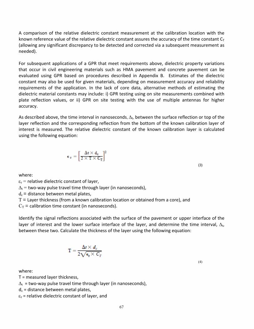
67
A comparison of the relative dielectric constant measurement at the calibration location with the known reference value of the relative dielectric constant assures the accuracy of the time constant CT (allowing any significant discrepancy to be detected and corrected via a subsequent measurement as needed). For subsequent applications of a GPR that meet requirements above, dielectric property variations that occur in civil engineering materials such as HMA pavement and concrete pavement can be evaluated using GPR based on procedures described in Appendix B. Estimates of the dielectric constant may also be used for given materials, depending on measurement accuracy and reliability requirements of the application. In the lack of core data, alternative methods of estimating the dielectric material constants may include: i) GPR testing using on site measurements combined with plate reflection values, or ii) GPR on site testing with the use of multiple antennas for higher accuracy.
As described above, the time interval in nanoseconds, t, between the surface reflection or top of the layer reflection and the corresponding reflection from the bottom of the known calibration layer of interest is measured. The relative dielectric constant of the known calibration layer is calculated using the following equation:
(3) where:
r = relative dielectric constant of layer, t = two‐way pulse travel time through layer (in nanoseconds), dc = distance between metal plates, T = Layer thickness (from a known calibration location or obtained from a core), and CT = calibration time constant (in nanoseconds). Identify the signal reflections associated with the surface of the pavement or upper interface of the
layer of interest and the lower surface interface of the layer, and determine the time interval, t, between these two. Calculate the thickness of the layer using the following equation:
(4)
where: T = measured layer thickness,
t = two‐way pulse travel time through layer (in nanoseconds), dc = distance between metal plates,
r = relative dielectric constant of layer, and

68
CT = calibration time constant (in nanoseconds). REPORT: Quality control/quality assurance results obtained for the CT calibration value using the above procedure should be reported and evaluated based on comparison with known reference calibration values. If the measured value of the relative dielectric constant of the layer determined using CT is within acceptable measurement tolerances at the known calibration location, measurement work with the GPR system may proceed. A report should be provide analysis results in graphical and/or bar chart forms based on referenced analysis steps in Appendix B. Pavement layer thickness results can be reported versus mile post for analysis of overall variability. Statistical variability of pavement layer thickness within homogeneous pavement sections can be specifically reported using procedures in Appendix B.

69
APPENDIX A. (from ASTM 4748 and SHRP2 Report S2‐R06C‐RR1)
TIME CONSTANT, CT, CALIBRATION The calibration of the time constant, CT, is established by measuring the time interval between reflections from two metal plates spaced by a distance, dc, of approximately 300 ±5 mm (12 ± 0.2 in.) using four small non‐conductive spacers, one attached to each corner of the metal plates, Figure 1. The upper plate is approximately 125 by 125mm (5 by 5 in.) and the lower plate is approximately 300 by 300 mm (12 by 12 in.). The time delay between the two reflections from the pair of plates by observing the received signal on the display device represents the time constant, CT, in nanoseconds, Figure 2. CT accuracy can be refined further using the following procedure modification: (a) collect a GPR waveform measurement corresponding to the upper metal plate, (b) remove the upper metal plate and nonconductive spacers from the measurement area, and (c) measure a GPR waveform corresponding to the lower metal plate alone. A modified procedure CT value (with higher accuracy) is obtained by calculating the time difference between the peak response in waveform “c” and the peak response in waveform “a.”
Figure 1. Time Constant, CT, Calibration Setup (ASTM 4748)

70
Figure 2. Time Constant, CT, Measurement (ASTM 4748) SIGNAL CALIBRATION Perform the following calibration and signal stability measurements (SHRP2 Report S2‐R06C‐RR1)

71

72

73
APPENDIX B. EXAMPLE DATA ANALYSIS:
Step 1. Perform manufacturer recommended GPR data pre‐processing steps such as the following:
a. Adjust zero time offset (focus analysis on target data time window) b. Subtract average background response c. Apply appropriate signal gain for material (linear, piecewise linear, exponential, etc.)
to achieve signal processing and analysis objectives by equalizing dynamic range as a function of depth
Step 2. Perform semi‐automated GPR pavement layer processing in manufacturer software and initially evaluate pavement thickness based on estimated dielectric properties (material specific [Daniels, 1996]).
Step 3. Import initial GPR thickness data into MS Excel to perform multi‐scale data analysis and statistical analysis procedures using an ADOJAM MS Excel Macro.
a. Import pre‐processed GPR thickness data into macro spreadsheet
i. Estimated pavement thickness information is imported layer by layer ii. Measured pavement core layer thickness is entered manually
b. Execute spreadsheet macro provided by ADOJAM to analyze layer features at multiple length scales (multi‐scale data analysis)
i. Compare statistical results from large scales down to successively smaller length scales to determine homogeneous length scales of data subsections (where layers can be consistently identified, Figure 1). In Figures 2 and 3, homogeneous subsection statistics are highlighted in yellow when statistical thickness criteria have been met and are subsequently highlighted in green upon further subdivision.
ii. Multi‐scale data analysis criteria (user adjustable to address specific needs) include:
i. Maximum difference between average pavement layer thickness of adjacent data subsections (layer by layer)
ii. Maximum difference between the standard deviation of pavement layer thickness of adjacent data subsections (layer by layer)
iii. After minimum length scale subdivisions have been reached, define a minimum standard deviation (or a complete lack of detected data features) within a data subsection to identify a subsection transition zone.

74
Step 4. Use results from Step 3 in an ADOJAM macro to produce results for decision making (example figures developed using MD SHA data)
a. Use existing MD SHA plotting spreadsheet to plot thickness results
b. Extract thickness statistics of each pavement layer at homogeneous length scales, determined in Step 3.b. (Figures 2 and 3, plus Table 1)
i. Mean ii. Standard deviation
c. Produce statistical summary for MD SHA analysis of i. Pavement layer thickness (at homogenous length scales) ii. Pavement layer thickness variability (at homogenous length scales)

75
Figure 1. Multi‐scale data analysis showing homogeneous pavement subsections for pavement layer
1 and pavement layer 2 based on current MD SHA GPR pavement layer analysis.
Figure 2. Multi‐scale analysis structure shown in ADOJAM MS Excel macro(zoom in view).

76
Figure 3. Multi‐scale analysis structure shown in ADOJAM MS Excel (zoom out view).
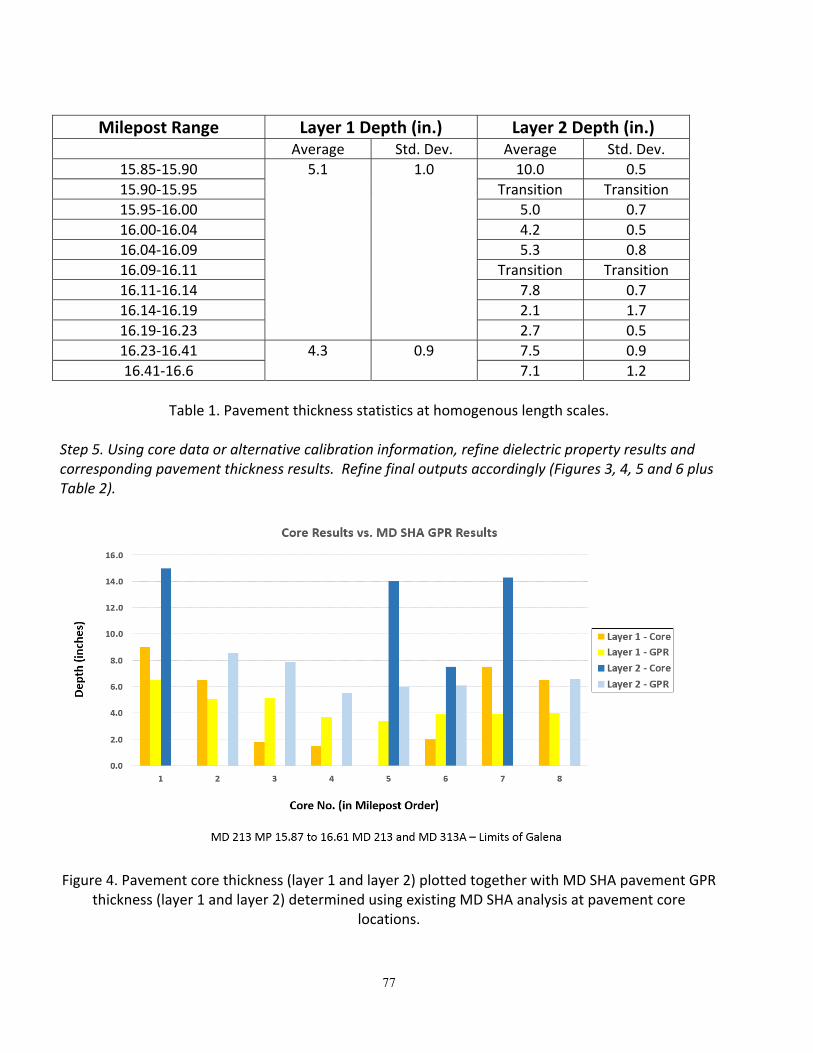
77
Milepost Range Layer 1 Depth (in.) Layer 2 Depth (in.) Average Std. Dev. Average Std. Dev.
15.85‐15.90 5.1 1.0 10.0 0.5
15.90‐15.95 Transition Transition
15.95‐16.00 5.0 0.7
16.00‐16.04 4.2 0.5
16.04‐16.09 5.3 0.8
16.09‐16.11 Transition Transition
16.11‐16.14 7.8 0.7
16.14‐16.19 2.1 1.7
16.19‐16.23 2.7 0.5
16.23‐16.41 4.3 0.9 7.5 0.9
16.41‐16.6 7.1 1.2
Table 1. Pavement thickness statistics at homogenous length scales.
Step 5. Using core data or alternative calibration information, refine dielectric property results and corresponding pavement thickness results. Refine final outputs accordingly (Figures 3, 4, 5 and 6 plus Table 2).
Figure 4. Pavement core thickness (layer 1 and layer 2) plotted together with MD SHA pavement GPR
thickness (layer 1 and layer 2) determined using existing MD SHA analysis at pavement core locations.

78
Figure 5. Present GPR thickness measurement error with respect to pavement core results based on
existing MD SHA analysis procedure at eight core locations.
Figure 6. Residual errors after proposed analysis of GPR results and pavement core results (designed to minimize error).
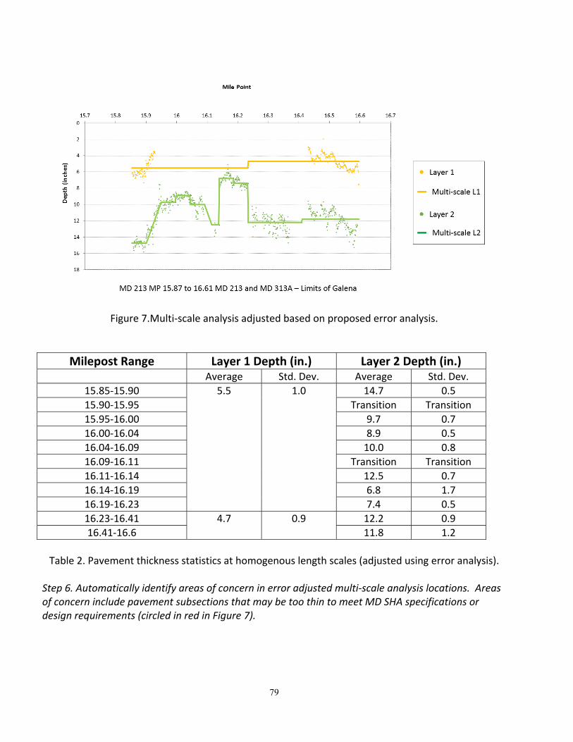
79
Figure 7.Multi‐scale analysis adjusted based on proposed error analysis.
Milepost Range Layer 1 Depth (in.) Layer 2 Depth (in.) Average Std. Dev. Average Std. Dev.
15.85‐15.90 5.5 1.0 14.7 0.5
15.90‐15.95 Transition Transition
15.95‐16.00 9.7 0.7
16.00‐16.04 8.9 0.5
16.04‐16.09 10.0 0.8
16.09‐16.11 Transition Transition
16.11‐16.14 12.5 0.7
16.14‐16.19 6.8 1.7
16.19‐16.23 7.4 0.5
16.23‐16.41 4.7 0.9 12.2 0.9
16.41‐16.6 11.8 1.2
Table 2. Pavement thickness statistics at homogenous length scales (adjusted using error analysis).
Step 6. Automatically identify areas of concern in error adjusted multi‐scale analysis locations. Areas of concern include pavement subsections that may be too thin to meet MD SHA specifications or design requirements (circled in red in Figure 7).

80
Figure 8. Layer 2 areas of concern circled in red.

81
APPENDIX C
MULTI‐SCALE ANALYSIS MACRO ALGORITHM For “Lyr” = 1 to # of pavement layer interfaces
Partition current “Lyr” thickness data equally into “part 1” and “part 2” per milepost location Compute average “part 1” thickness, “L#P1a” Compute average “part 2” thickness, “L#P2a” Compute “part 1” thickness standard deviation, “L#P1sd” Compute “part 2” thickness standard deviation, “L#P2sd” If ABS(L#P1a‐L#P2a) < Threshold average (user specified) Store “L#P1a” and “L#P2a” values and EndIf Else Subdivide current “Lyr” # into equally into parts, “p1i,” “p2i,” “p3i,” and “p4i” Compute average “p1i” thickness, “L#P1ia” Compute average “p2i” thickness, “L#P2ia”
Compute “p1isd” thickness standard deviation, “L#P1isd” Compute “p2isd” thickness standard deviation, “L#P2isd”
If ABS(L#P1ia‐L#P2ia) < Threshold average (user specified) Store “L#P1ia” and “L#P2ia” values and EndIf
Else Else subdivide current “Lyr” # subpart equally into four parts and evaluate subparts consistent with established pattern
EndIf Compute average “p3i” thickness, “L#P3ia” Compute average “p4i” thickness, “L#P4ia” Compute “p3i” thickness standard deviation, “L#P3isd” Compute “p4i” thickness standard deviation, “L#P4isd”
If ABS(L#P3ia‐L#P4ia) < Threshold average (user specified) Store “L#P3ia” and “L#P4ia” values and EndIf
Else If AVERAGE(p3isd,p4isd) > Threshold st dev (user specified) or null (and minimum subdivision length scale has been reached)
Categorize as “transition” area Else
Subdivide current “Lyr” # subpart equally into eight parts, evaluate subparts consistent with established pattern until all segments have been categorized
EndIf EndIf Endif Next

82
Approval:
Maryland Department of Transportation
State Highway Administration
Office of Materials Technology
MARYLAND STANDARD METHOD OF TESTS
Approved:
GPR FOR BRIDGE DECKS
MSMT
xxx
SCOPE:
This procedure is used to determine the condition of concrete bridge decks. Specifically, this this
non‐destructive evaluation method could identify defects related to concrete and rebar
deterioration.
REFERENCE DOCUMENTS:
ASTM D6087‐08, “Evaluating Asphalt‐Covered Concrete Bridge Decks Using Ground Penetrating
Radar.”
ASTM D6432‐11, “Standard Guide for Using the Surface Ground Penetrating Radar Method for
Subsurface Investigation.”
AASHTO, “Standard Practice for Application of Ground Penetrating Radar (GPR) to Highways,” Report
No. R037‐04‐UL, 2009, pp. 12.
ACI 228.2R‐13 “Report on Nondestructive Test Methods for Concrete in Structures,” American
Concrete Institute, June 2013, pp. 53‐61.
Daniels, D.J., Surface Penetrating Radar, The Institution of Electrical Engineers, pp. 320, December
1996.
Scott, M.L., Nondestructive Testing Handbook, 3rd Edition, Volume 5, Electromagnetic Testing,
Chapter 17. Infrastructure Applications, Part 2. Applications of Ground Penetrating
Radar to Bridge Decks, American Society of Nondestructive Testing, 2004, pp. 430‐436.
Scott, M., Rezaizadeh, A., Moore, M., “Phenomenology Study of HERMES Ground Penetrating Radar
Technology for Detection and Identification of Common Bridge Deck Features,” Report
FHWA‐RD‐01‐090, Federal Highway Administration, McLean, VA, 2001, pp 1‐27.

83
TERMINOLOGY:
Antenna is a transmitting GPR antenna that converts an excitation in the form of a voltage pulse or
wave train into EM waves. A receiving GPR antenna converts energy contained in EM waves into
voltages, which are regarded as GPR data upon digital sampling of analog voltages, and storage of
quantized values.
Bistatic Antenna is an antenna configuration that incorporates two antennas, where the first antenna
radiates incident EM waves toward the ground and the second antenna receives the reflected waves.
Bandwidth is the operating frequency range of an antenna, typically the difference between the
upper and lower 3‐dB frequencies (i.e., upper and lower 3 dB frequencies relative to the antenna’s
resonant frequency).
Coupling between the GPR antenna and the ground is indicated by the efficiency of the antenna
transmitting electromagnetic energy into the ground, where “good” coupling is indicated by efficient
transmission of EM energy from the antenna into the ground within the antenna bandwidth and
“poor” coupling is indicated by low efficiency transmission of EM energy from the antenna into the
ground within the antenna bandwidth.
Depth of Penetration is the maximum depth range a radar signal can penetrate into a given material.
Attenuation is the loss of EM wave energy due to conduction currents.
Scattering is the change in direction of electromagnetic wave propagation that occurs at a change in
material properties over a short distance compared to a wavelength for an interval comparable to or
greater than a wavelength. Scattering includes reflection (reverse change in direction), refraction
(forward change in direction), and diffraction (caused by rapid changes that are small compared to a
wavelength in both occurrence and interval).
84
Time gain is the amplification applied to a trace as a function of time, where the function can be
continuous or piecewise depending on data analysis requirements.
Transmit Pulse is the voltage impulse that excites the transmitting antenna.
Polarization (polarization vector) is the orientation of the direction of the vector electromagnetic
field. Many GPR antennas are linearly polarized.
Conductivity is the ability of a material to support movement of electrons or ions due to an applied
electrical field.
Diffusion is the movement of charges in response to an applied electric field or in response to an
applied time‐varying magnetic field. Diffusion is the low‐frequency, high‐loss, limiting behavior of
electromagnetic wave propagation and is descriptive of behavior that decays rapidly (exponentially)
with distance and time.
Dispersion is a material characteristic where wave velocity is no longer uniquely defined, giving rise
to the distinction of phase velocity and group velocity. For example, elevated water content in
dielectric civil engineering materials (such as concrete and asphalt) results in increased dispersion
effects, where electromagnetic waves become increasingly spread out as a function of frequency.
Dielectric Permittivity is the property that describes the ability of a material to store electric
energy by separating opposite polarity charges in space. It relates ability of a material to be polarized
in response to the application of an electric field.
Relative Permittivity (relative dielectric permittivity; Dielectric Constant) is the ratio of the dielectric
permittivity of a material to the permittivity of free space (or vacuum).

85
Magnetic Permeability (μ) is the property that describes the ability of a material to store magnetic
energy by realignment of electron spin and motion. It relates ability of a material to be magnetized
(magnetic polarization).
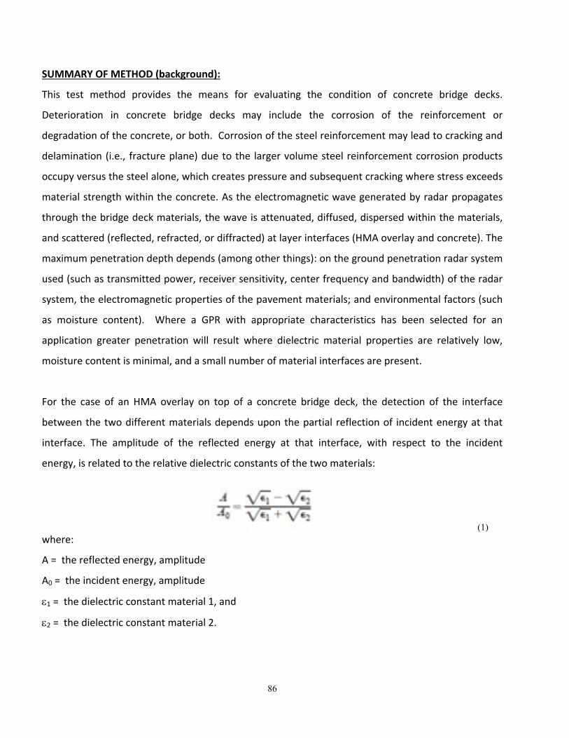
86
SUMMARY OF METHOD (background):
This test method provides the means for evaluating the condition of concrete bridge decks.
Deterioration in concrete bridge decks may include the corrosion of the reinforcement or
degradation of the concrete, or both. Corrosion of the steel reinforcement may lead to cracking and
delamination (i.e., fracture plane) due to the larger volume steel reinforcement corrosion products
occupy versus the steel alone, which creates pressure and subsequent cracking where stress exceeds
material strength within the concrete. As the electromagnetic wave generated by radar propagates
through the bridge deck materials, the wave is attenuated, diffused, dispersed within the materials,
and scattered (reflected, refracted, or diffracted) at layer interfaces (HMA overlay and concrete). The
maximum penetration depth depends (among other things): on the ground penetration radar system
used (such as transmitted power, receiver sensitivity, center frequency and bandwidth) of the radar
system, the electromagnetic properties of the pavement materials; and environmental factors (such
as moisture content). Where a GPR with appropriate characteristics has been selected for an
application greater penetration will result where dielectric material properties are relatively low,
moisture content is minimal, and a small number of material interfaces are present.
For the case of an HMA overlay on top of a concrete bridge deck, the detection of the interface
between the two different materials depends upon the partial reflection of incident energy at that
interface. The amplitude of the reflected energy at that interface, with respect to the incident
energy, is related to the relative dielectric constants of the two materials:
(1) where:
A = the reflected energy, amplitude
A0 = the incident energy, amplitude
1 = the dielectric constant material 1, and
2 = the dielectric constant material 2.

87
The ability to detect the overlay thickness of a layer depends on the contrast between the dielectric
constant of the overlay and the concrete bridge deck beneath. Overlay thickness can be determined
using radar technology if the dielectric constant of that material and the two‐way travel time for the
radar wave to pass through the layer are known. The relationship is defined by the following
equation:
(2) where:
T = overlay thickness,
c = speed of light in air, 300 mm/nsec for T in mm (11.8 in/nsec for T in inches),
r = relative dielectric constant of layer, and
t = two‐way pulse travel time through layer (in nanoseconds).
The dielectric constant of a pavement material can vary within a typical range depending on
aggregate types, asphalt cement sources, density, cracking, voids, foreign matter, moisture content,
and other less common variables. Using an air‐coupled horn antenna radar the real part of this
variation may be calculated directly from the radar data by using the known dielectric constant of air
and equation (1).
Determining the dielectric constant when using ground coupled dipole antenna radar requires an
independent means, such as coring, or a radar based dielectric constant measurement. Radar based
dielectric constant measurements can be performed using multi‐static antenna pairs positioned at
two or more transmitter to receiver location offsets. Using this approach, material properties are
subsequently analyzed with techniques such as the Common Midpoint (CMP) method.
APPARATUS:
Two alternative GPR systems may be used for this evaluation:
‐ Air‐coupled antennas with central frequencies 1 GHz and greater, with control unit able to
transmit at a sufficient rate to collect 20 scans/m (25 scans/ft). The equipment may consist of
88
either an air‐coupled, short‐pulse monostatic or bistatic radar(s) with a monocycle pulse 150
mm (6 in.) free space resolution and a 50 scan/s minimum data rate.
‐ Ground‐coupled antennas with central frequencies greater than 1 GHz with control unit able
to transmit at a sufficient rate to collect 80 scans/m.
The data acquisition system should be able to gather radar data at the minimum rate of the radar
system(s), 50 kHz for one radar, 100 kHz for two radars, and 150 kHz for three radars. The system
shall be capable of accurately acquiring radar data with a 60‐dB dynamic range. A distance
measurement instrument (DMI) with accuracy of 6100 mm/km (66.5 in./mile) and a resolution of 25
mm (1 in.) should be used.
PERIODIC CALIBRATION
For air coupled systems perform calibration and stability measurement procedures (such as signal‐to‐
noise ratio, signal stability, long‐term signal stability tests) as described in Appendix A.
PRE‐OPERATION MEASUREMENTS:
Free Space Signal (FSP): The equipment manufacturer may require the radar antenna to be mounted
in an operational configuration, and 100 waveforms gathered in the absence of the material to be
inspected. Use the average of 100 waveforms as a template for clutter removal.
Flat Metal Plate (FMP): Position the radar in an operation configuration, and gather 100 waveforms
while illuminating a flat plate with dimensions recommended by the manufacturer. This is a measure
of the emitted energy to be used in subsequent measurements, and as a template for correlation or
background removal, or both.
DATA COLLECTION PROCEDURE:
Air‐Coupled Systems:
89
‐ Make radar inspection passes in a longitudinal direction parallel to the centerline of the
bridge deck with the antenna mounted to maintain a manufacturer‐recommended distance
from the bridge deck surface.
‐ Use a transverse distance (dt) between radar inspection passes <1 m (3 ft).
‐ Use a longitudinal distance (dl) between radar scans <150 mm (6 in).
‐ Determine the starting location for passes, that is, at abutments, joints, or a predetermined
location.
‐ Determine the speed of operation for contiguous longitudinal coverage based on the radar
range sweep rate and the manufacturer‐recommended scan‐spacing.
Ground‐Coupled Systems:
‐ Make radar inspection passes either parallel or perpendicular to the direction of traffic,
depending on the direction of the top layer of reinforcing. The pass direction should be
chosen so that the antenna crosses over the top layer of reinforcing at an angle nearest to
90°.
DATA ANALYSIS:
Two different data processing methodologies are commonly used based on reflection amplitudes.
The first method, the “attenuation technique,” calculates deterioration based on the relative
reflection amplitudes from the bridge deck bottom relative to the bridge deck surface. The second
method, the “top reinforcing reflection technique,” utilizes the relative reflection amplitudes from
the top layer of reinforcing to assess deterioration.
Deterioration Measurements at Top Reinforcing Steel—Attenuation Technique:
‐ Measure and record the applied signal strength, Vt, at the deck surface.
‐ Measure and record the maximum signal strength of the deck bottom echo, Vbs.

90
‐ If Vbs is < 0.0264 Vt after repeating the longitudinal radar inspection pass, the data are not
reliable for determining removal quantities of bridge deck concrete. Processing of the data
will require an alternative technique (such as the one used by the Ontario Ministry of
Transportation).
‐ Measure and record the amplitude of the deck bottom echo, Vb, for each waveform.
‐ Determine delamination at the top reinforcing steel using the attenuation technique as
follows:
o Consider the concrete delaminated if: Vb ≤ 0.385 Vbs
where: Vb = bottom echo amplitude, each scan; Vbs = bottom echo maximum
amplitude, all scans; and 0.385 = a constant derived from research data.
o Calculate the percent delaminated at the top steel in each radar inspection pass using
the following:
Xtn = [ [Wdt)/(Wdt + Wst) ] [100] (3)
where: Xtn = percent delaminated in a radar inspection pass n, at top steel; n = radar
inspection pass identification number; Wdt = concrete delaminated at top steel, m;
and, Wst = sound concrete at top steel, m.
o Calculate the estimated quantity of deck delaminated at top steel for each radar
inspection pass using the following:
Qt = (Xtn) (Ln) (dt) (4)
where: Qt = square meters (feet) of deck delaminated at top steel; Ln = length of radar
inspection pass, n, m; and dt = transverse distance between radar inspection passes,
m.

91
o Calculate the total estimated quantity of deck delaminated at top steel using the
following:
Q Tt = Qt (5) where: QTt = total square meters (feet) of deck delaminated at top steel for all radar
inspection passes.
Deterioration Measurements at or above Top Reinforcing Steel—Top Reinforcing Reflection
Technique:
‐ Extract the reflection amplitudes from the top layer of reinforcing.
Air‐Coupled System:
Data collected with the air‐coupled system should be obtained with two antennas (a transmitter and
receiver pair) positioned in‐line with the longitudinal direction and radiating with a polarization
orientation perpendicular to the transverse reinforcing steel direction. The first step in data
processing involves clutter removal by normalizing the reflection amplitudes of the metal plate
reflections to the asphalt reflection (when HMA overlay exist), then subtracting the free space (FSP)
scan from each data scan starting at the mid‐point of the asphalt surface reflection. This method may
not be reliable for bridge decks containing longitudinal rebar on top of transverse rebar with on‐
center spacing less than 20 cm (8 in.). For this situation, ground‐coupled antenna data should be
collected in the direction transverse to traffic flow in addition to longitudinal ground‐coupled data,
data should be collected and evaluated using the “attenuation technique” or cross‐polarized GPR
antenna methods may be implemented.
If the orientation of the top layer of reinforcing is not skewed at close to 45° relative to the direction
of traffic: (a) normalize the asphalt reflection amplitude of the antenna polarized parallel to the top
layer of reinforcing relative to (b) the same reflection amplitude in the other antenna and subtract
(b) from (a) for each data scan. This is done to isolate the reflection from the top layer of reinforcing
from the asphalt bottom reflection. For top layer of reinforcing angles near 45°, no subtraction
should be performed. However, for this case, if the reinforcing reflection amplitudes cannot visually
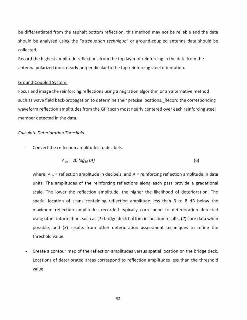
92
be differentiated from the asphalt bottom reflection, this method may not be reliable and the data
should be analyzed using the “attenuation technique” or ground‐coupled antenna data should be
collected.
Record the highest amplitude reflections from the top layer of reinforcing in the data from the
antenna polarized most nearly perpendicular to the top reinforcing steel orientation.
Ground‐Coupled System:
Focus and image the reinforcing reflections using a migration algorithm or an alternative method
such as wave field back‐propagation to determine their precise locations. Record the corresponding
waveform reflection amplitudes from the GPR scan most nearly centered over each reinforcing steel
member detected in the data.
Calculate Deterioration Threshold.
‐ Convert the reflection amplitudes to decibels.
Adb = 20 log10 (A) (6)
where: Adb = reflection amplitude in decibels; and A = reinforcing reflection amplitude in data
units. The amplitudes of the reinforcing reflections along each pass provide a gradational
scale. The lower the reflection amplitude, the higher the likelihood of deterioration. The
spatial location of scans containing reflection amplitude less than 6 to 8 dB below the
maximum reflection amplitudes recorded typically correspond to deterioration detected
using other information, such as (1) bridge deck bottom inspection results, (2) core data when
possible, and (3) results from other deterioration assessment techniques to refine the
threshold value.
‐ Create a contour map of the reflection amplitudes versus spatial location on the bridge deck.
Locations of deteriorated areas correspond to reflection amplitudes less than the threshold
value.

93
‐ Calculate the percent deterioration at or above the top steel in each radar inspection pass
using the following:
Xtn = [ [Wdt)/(Wdt + Wst) ] [100] (7)
where: Xtn = percent deteriorated in a radar inspection pass, n, at or above top steel; n =
radar inspection pass identification number; Wdt = concrete deteriorated at or above top
steel, m, obtained from reflection amplitudes below deterioration threshold value; and Wst =
sound concrete at top steel, m, obtained from reflection amplitudes above the deterioration
threshold value.
‐ Estimate the quantity of deck deteriorated at or above the top reinforcing using equations 4 and 5.
REPORT:
Report should provide bridge identification and location, survey date and weather conditions, deck
status relative to moisture and debris, and any unusual conditions or circumstances. In terms of radar
results, the report should include:
‐ Percent of bridge deck area delaminated, otherwise distressed, or defective for each radar
pass, at top steel, in tabular form;
‐ Bridge deck area, in square meters (feet) delaminated, otherwise distressed, or defective for
each radar pass, at top steel, in tabular form;
‐ Total bridge deck area, in square meters (feet), delaminated, otherwise distresses, or
defective for the bridge deck, at top steel, in tabular form;
‐ Plan view map of bridge deck, depicting radar inspection pass versus longitudinal distance
and showing location and extent of detected delamination, other distress, or defects at
top steel; and,
‐ Plan view map of cover depth corresponding to the top layer of bridge deck reinforcing
steel.

94
APPENDIX A. (per ASTM D6087)
SYSTEM PERFORMANCE COMPLIANCE
1. Signal‐to‐Noise Ratio Test: Position the antenna at its far field distance approximately equal to
maximum dimension of antenna aperture above a square metal plate with a width of 4 times the
antenna aperture, minimum. Turn on the radar unit and allow to operate for a 20‐min warm‐up
period or the time. After warming up the unit, record 100 waveforms. Then evaluate the recorded
waveform for signal‐to‐noise ratio. The signal‐to‐noise ratio is described by the following equation:
[Signal Level ( Amp ) / Noise Level (An ) ] > 20 (26.0 dB)
This will be performed on each of the 100 waveforms and the average signal‐to‐noise value of the
100 waveforms will be taken as the “signal‐to‐noise of the system.” Noise voltage (An) is defined as
the maximum amplitude occurring between metal plate reflection and region up to 50 % of the time
window after the metal plate reflection, normally used with the antenna (that is, 1.0 GHz/20 ns: 10
ns.). The signal level (Amp) is defined as the amplitude of the echo from the metal plate. 6.2.1.3 The
signal‐to‐noise ratio test results for the GPR unit should be greater than or equal to 20 (+26.0 dB).
2. Signal Stability Test: Use the same test configuration as described in the signal‐to‐noise ratio
test. Record 100 traces at the maximum data acquisition rate. Evaluate the signal stability using the
following equation:
[ Amax – Amin / Aavg ] ≤ 0.01 (1%)
where:
Amax = the maximum amplitude of the metal plate reflection for all 100 traces,
Amin = the minimum amplitude of the metal plate reflection for all 100 traces, and
Aavg = the average trace amplitude of all 100 traces.
The signal stability test results for the GPR system should be less than or equal to 1 %.

95
3. Variations in Time Calibration Factor: Use the same test configuration as described in the signal‐
to‐noise ratio test, except that the metal plate can be replaced by any reflecting object. Collect a
single waveform and measure the distance from the antenna to the reflector. Perform this test at
three different distances corresponding to approximately 15, 30, and 50 % of the time window
normally used with the system. The time delay between the echo from the aperture of the
transmitting antenna and that from the reflecting object is measured as time t1 (where subscript 1
represents position 1, and so forth). The difference between t2 and t1 and between t3 and t2
represents the travel time for a fixed distance in air. The factor Ci represents the speed between
distance i and i+1. The allowable variation in measured speed is shown as follows:
[ C1 – C2 / Mean of C1 and C2] ≤ 0.02 (2%)
where:
C1 = distance from Position 2 to Position 1/ t1
C2 = distance from position 3 to Position 2 / t2
The variation in time calibration factor should be less than 2 %.
4. Long‐Term Amplitude Variation: Use the same test configuration as described in the signal‐to‐
noise ratio test. Switch on the radar and allow to operate for 2 h continuously. As a minimum,
capture a single waveform every 1 min, 120 total. Calculate the amplitude of a metal plate reflection
and plot against time for each waveform. For the system to perform adequately, the amplitude of
reflection should remain constant after a short warm‐up period. The stability criteria is as follows:
[ Amax – A20 / A20 ] ≤ 0.03 (3%)
Amax = the largest amplitude measured between 20 min and 120 min.
A20 = the amplitude measured after 20 min.

96
APPENDIX B TRAINING MODULES

97

98

99

100

101

102

103

104

105

106

107

108

109

110
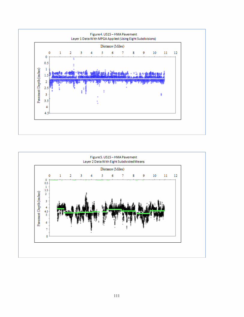
111

112

113
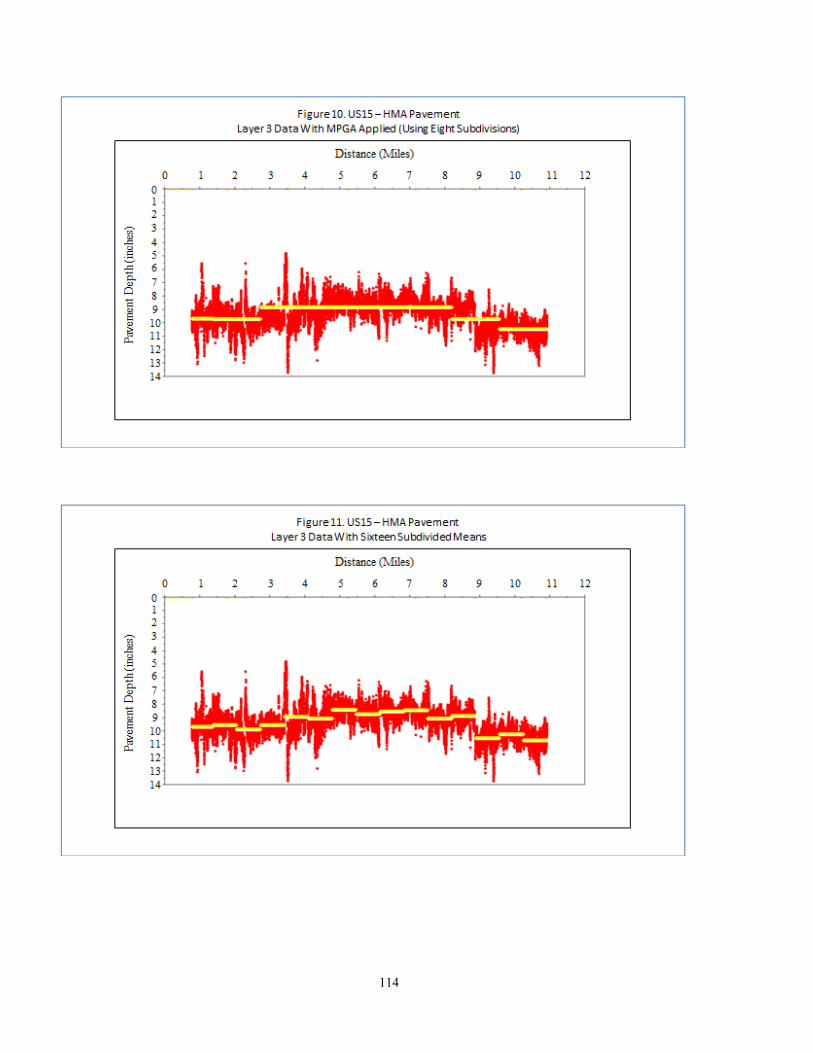
114

115
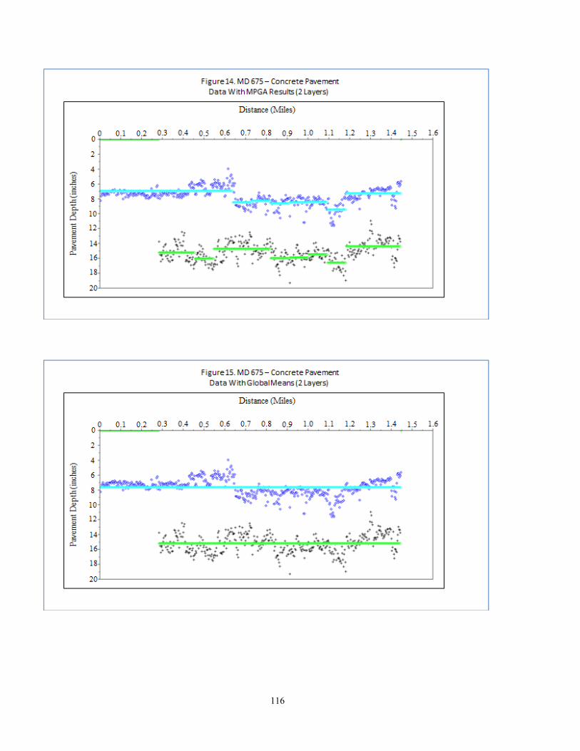
116
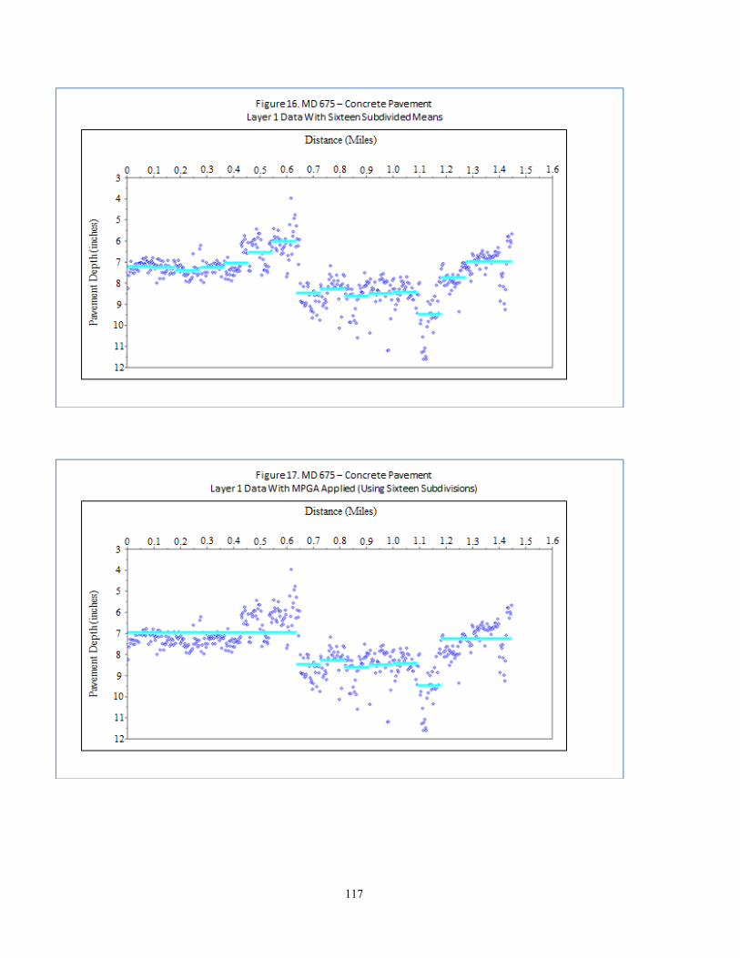
117

118

119

120

121

122

123

124

125

126

127

128

129

130

131

132
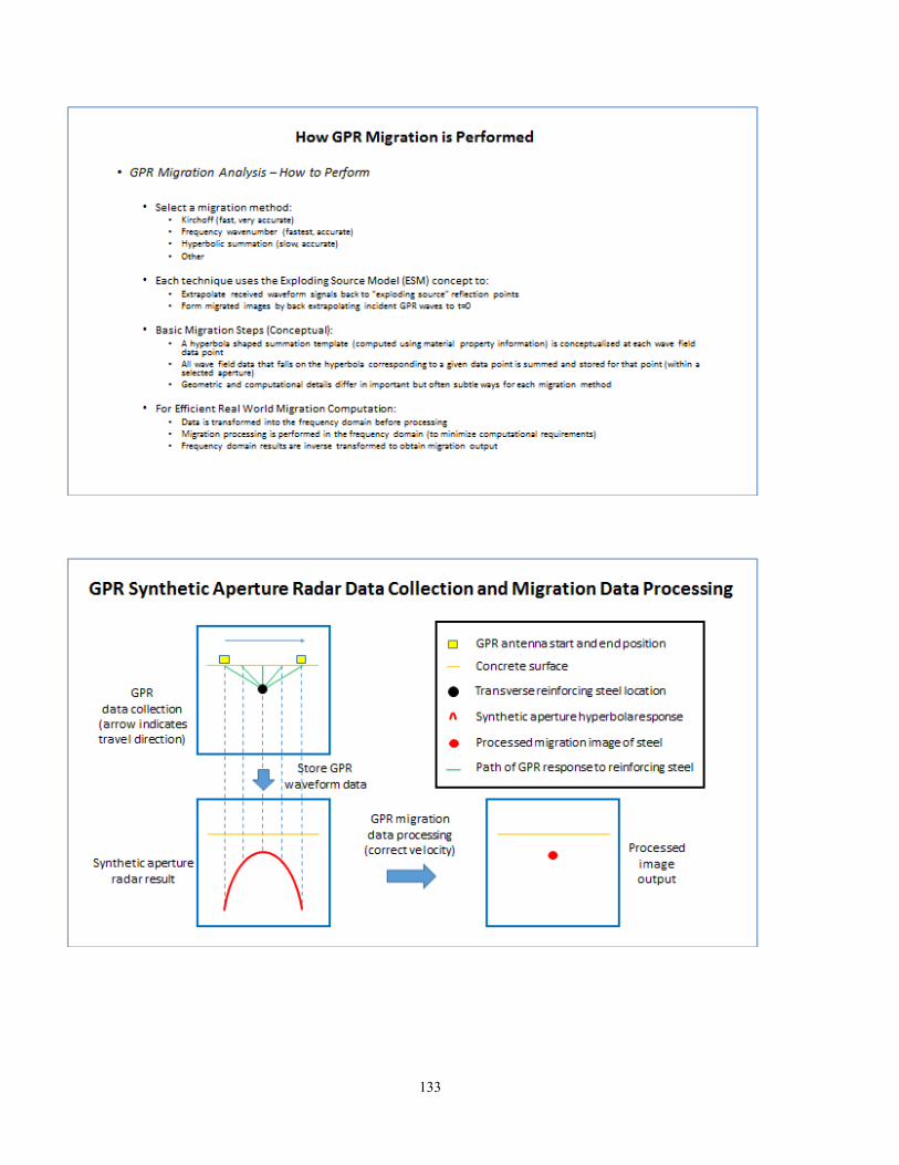
133

134

135

136

137

138

139

140
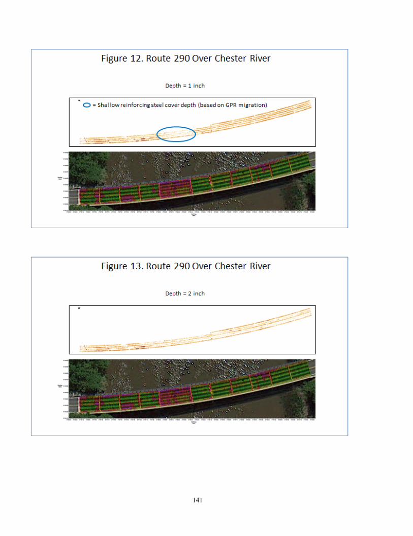
141
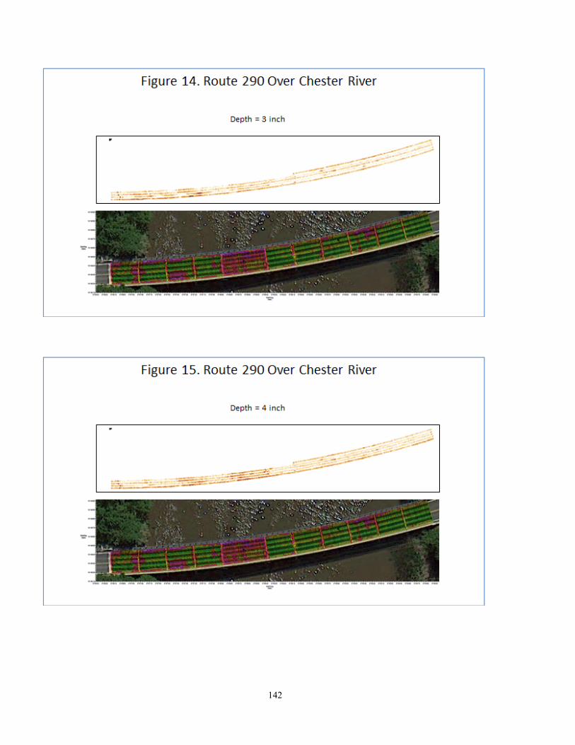
142

143

144
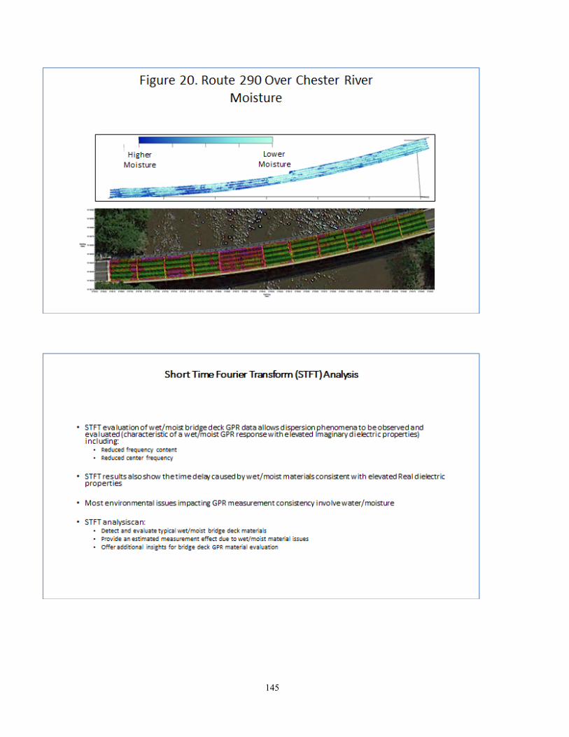
145
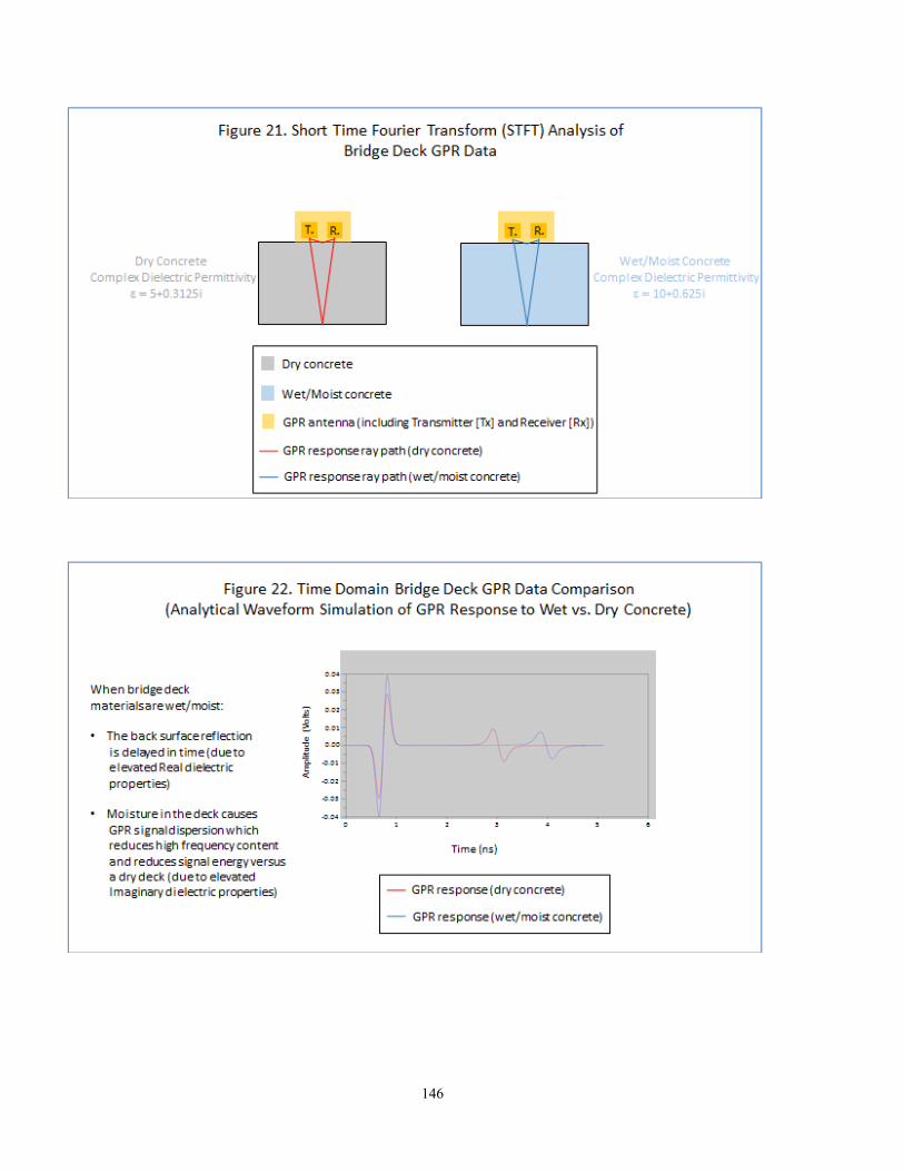
146

147

148

149

150

151
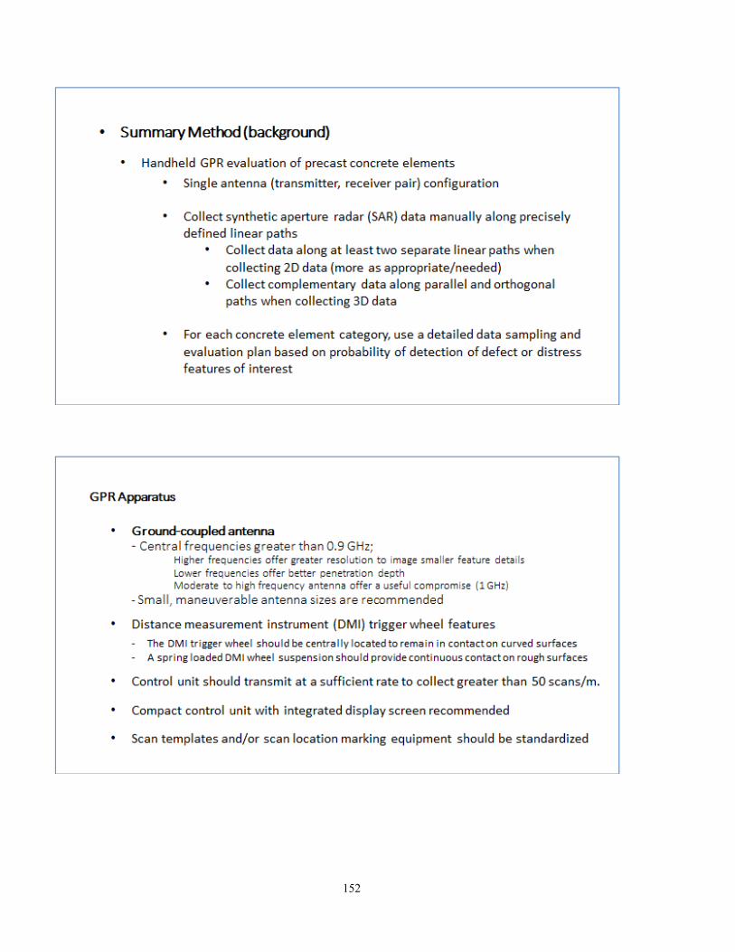
152

153

154

155

156
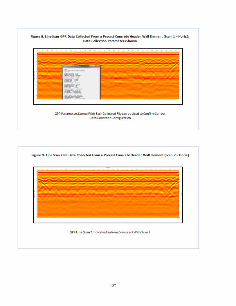
157

158

159

160

161

162

163
APPENDIX C SCI-LAB SCRIPT

164
The SciLab script code beta version 3 is composed of an executable file (MSA25.sce and two custom functions (compsrcipt1.sci and Rmsf2.sci) called by the executable file. The purpose of each script is described next.
1. MSA25.sce SciLab executable script. Purpose: Evaluates and summarizes GPR pavement layer data trends and features using automated or semi‐automated techniques. //* Multi Scale Analysis (Revision 3 Beta) //* //* Purpose: //* Evaluates and summarizes GPR pavement layer data trends and //* features using automated or semi-automated techniques //* //* Inputs: //* Milepost data filename: pathai definition (Line 24) //* Layer1 depth data filename: patha definition (Line 25) //* Layer2 depth data filename: pathb definition (Line 26) //* Layer3 depth data filename: pathc definition (Line 26) //* //* Final Output: //* Plot presenting multi-scale results corresponding to three //* GPR pavement data layers //* //* User adjustable parameters: //* 1. path = Current directory (where all data files, executables //* and subroutines are stored) //* 2. initsub = number of multi-scale analysis (MPGA) subdivisions //* desired by the user for analysis mode(0) clear all; //**Adjust number of multi-scale subdivisions by defining initsub initsub=16.0; //**Change path string below to match directory selected path='C:\test\Rev3\'; //**Change file names to reflect input file names pathai='MP.csv'; patha='US15L1.csv'; pathb='US15L2.csv'; pathc='US15L3.csv'; //Set current directory to path cd(path); //Initialize *.sci functions to use as program subroutines funcprot(0); exec("rmsf2.sci"); exec("compcrit1.sci");

165
//Load Data Strings samp=35832; path1i=strcat([path,pathai]); fd_ri=mopen(path1i,'rt'); txti=mgetl(fd_ri, samp); //mprintf('%s\n',txt); di=strtod(txti); [di,endstr]=strtod(txti); clear(txti); erri=mclose([fd_ri]); path1=strcat([path,patha]); path2=strcat([path,pathb]); path3=strcat([path,pathc]); fd_r=mopen(path1,'rt'); txt=mgetl(fd_r, samp); //mprintf('%s\n',txt); d=strtod(txt); [d,endstr]=strtod(txt); clear(txt); err=mclose([fd_r]); fd_r2=mopen(path2,'rt'); txt2=mgetl(fd_r2, samp); //mprintf('%s\n',txt2); d2=strtod(txt2); [d2,endstr]=strtod(txt2); clear(txt2); err2=mclose([fd_r2]); fd_r3=mopen(path3,'rt'); txt3=mgetl(fd_r3, samp); //mprintf('%s\n',txt3); d3=strtod(txt3); [d3,endstr]=strtod(txt3); clear(txt3); err3=mclose([fd_r3]); //Threshold Values for Difference in Mean and Standard Dev Between Segments and initial subdivision size MeanDif1=0.3; StDevDif1=0.1; MeanDif2=0.3; StDevDif2=0.1; MeanDif3=0.3; StDevDif3=0.1;

166
szd=size(d); szdone=szd(1); szd2=size(d2); szd2one=szd2(1); szd3=size(d3); szd3one=szd3(1); //Initial Layer 1 Statistics (Full Data Set) x2=0; for x=1:szdone if isnan(d(x)) then d(x)=0; end if d(x)<>0|d(x)<>%nan then x2=x2+1; ds(x2)=d(x); end end [ij, v, mn]=spget(sparse(ds)); dstdev=stdev(v); dmean=mean(v); //Initial Layer 2 Statistics (Full Data Set) y2=0; for x=1:szd2one if isnan(d2(x)) then d2(x)=0; end if d2(x)<>0|d2(x)<>%nan then y2=y2+1; d2sa=d2(x); d2s(y2)=d2sa; end end [ij, v, mn]=spget(sparse(d2s)); dstdev2=stdev(v); dmean2=mean(v); //Initial Layer 3 Statistics (Full Data Set) z2=0; for x=1:szd3one if isnan(d3(x)) then d3(x)=0; end if d3(x)<>0|d3(x)<>%nan then z2=z2+1; d3sa=d3(x); d3s(z2)=d3sa;
167
end end [ij, v, mn]=spget(sparse(d3s)); dstdev3=stdev(v); dmean3=mean(v); // Filter significant layer crossover phenomena for x=1:szd2one if d2(x)<>0&d2(x)<dmean then d2(x)=0.; end end for x=1:szd3one if d3(x)<>0&d3(x)<dmean2 then d3(x)=0.; end end //Initial plot with three data layers and mean values presented for x=1:szdone if d(x)<>0 then mn1(x)=dmean; di1(x)=di(x); else mn1(x)=0.; end end for x=1:szd2one if d2(x)<>0 then mn2(x)=dmean2; di2(x)=di(x); else mn2(x)=0.; end end for x=1:szd3one if d3(x)<>0 then mn3(x)=dmean3; di3(x)=di(x); else mn3(x)=0.; end end //[dmeans,dmean2s,dmean3s,dstdvs,dstdv2s,dstdv3s]=substat(d,d2,d3);
168
figure(2); plot(di,d,'bd',di,d2,'k+',di,d3,'r.'); plot(di,mn1,'wd'); plot(di,mn2,'gd'); plot(di,mn3,'yd'); for x=1:szd3one // plot(di3,mn3,'y-'); end xlabel("Milepost"); ylabel("Depth (inches)"); //Initial Multi-Scale Subdivision Function Call - Layer 1 [L1subm,L1substd,mn1seg,std1seg]=rmsf2(szdone,initsub,di,d,MeanDif1,StDevDif1); figure(100); plot(di,d,'d'); plot(di,L1subm,'wd'); //Initial Multi-Scale Subdivision Function Call - Layer 2 [L2subm,L2substd,mn2seg,std2seg]=rmsf2(szd2one,initsub,di,d2,MeanDif2,StDevDif2); figure(101); plot(di,d2,'k+'); plot(di,L2subm,'gd'); //Initial Multi-Scale Subdivision Function Call - Layer 3 [L3subm,L3substd,mn3seg,std3seg]=rmsf2(szd3one,initsub,di,d3,MeanDif3,StDevDif3); figure(102); plot(di,d3,'r.'); plot(di,L3subm,'yd'); //Initial layer 1 subdivision criteria evaluation [L1submo1,mn1sega,std1sega,crit1,lbl]=compcrit1(szdone,mn1seg,std1seg,initsub,L1subm,MeanDif1,StDevDif1,dmean,dstdev); figure(200); plot(di,d,'d'); plot(di,L1submo1,'wd'); //Initial layer 2 subdivision criteria evaluation [L2submo2,mn2sega,std2sega,crit2,lbl2]=compcrit1(szd2one,mn2seg,std2seg,initsub,L2subm,MeanDif2,StDevDif2,dmean2,dstdev2); figure(400); plot(di,d2,'k+'); plot(di,L2submo2,'gd'); //Initial layer 1 subdivision criteria evaluation

169
[L3submo3,mn3sega,std3sega,crit3,lbl3]=compcrit1(szd3one,mn3seg,std3seg,initsub,L3subm,MeanDif3,StDevDif3,dmean3,dstdev3); figure(600); plot(di,d3,'r.'); plot(di,L3submo3,'yd'); //Plot final mult-scale output results figure(1000); plot(di,d,'bd',di,d2,'k+',di,d3,'r.'); plot(di,L1submo1,'wd'); plot(di,L2submo2,'gd'); plot(di,L3submo3,'yd');
2. compscrit1.sci Purpose: Evaluate multiscale phenomena based on statistical criteria at a user selected scale of interest. Consistent data trends and data variability are detected and passed to the main program script as output via the Lsubmo2 variable based on the analysis scale selected. function [Lsubmo2, mnsegn, stdsegn, crit, lbl]=compcrit1(sz, mnseg, stdseg, initsub, Lsubm, MeanDif1cr, StDevDif1cr, dmean, dstdev) //* Function call for MSA25.sce SciLab script //* //* Purpose: Evaluate multiscale phenomena based on statistical //* criteria at a user selected scale of interest. Consistent data //* trends and data variability are detected and passed to the main //* program script as output via the Lsubmo2 variable based on //* the analysis scale selected. //Evaluate initial segmented results versus multiscale criteria for xi=1:initsub mndif1=mnseg(xi)-dmean; stddif1=stdseg(xi)-dstdev; if mndif1<MeanDif1cr&stddif1<StDevDif1cr then mnsegn(xi)=dmean; stdsegn(xi)=dstdev; crit(xi)=1; else mnsegn(xi)=mnseg(xi); stdsegn(xi)=stdseg(xi); crit(xi)=0; end end incr=round(sz/initsub); sbst=0; lblinc=1;

170
for xi=1:initsub clear subset; clear mn1; clear std1; clear dep; sbst=sbst+incr; ref=1; if xi>1 then; ref=sbst-incr+1; end if xi==initsub then ref=sz-incr+1; sbst=sz; end for y=ref:sbst if Lsubm(y)<>0 then if crit(xi)==1 then Lsubmo(y)=dmean; lbl(y)=lblinc; else Lsubmo(y)=Lsubm(y); lbl(y)=0; end else Lsubmo(y)=0; lbl(y)=0; end end if crit(xi)==0 then lblinc=lblinc+1; lbl(y)=0; end end incr=round(sz/initsub); sbst=0; lblinc=1; for xi=1:initsub sbst=sbst+incr; ref=1; if xi>1 then; ref=sbst-incr+1; end if xi==initsub then ref=sz-incr+1; sbst=sz; end for y=ref:sbst if Lsubm(y)<>0 then if lbl(y)>=1 then lblcur=lbl(y);

171
vals(lblcur,y)=Lsubm(y); end end end end valsmn(1:lblcur)=0; incrm(1:lblcur)=0; incr=round(sz/initsub); sbst=0; for xi=1:initsub sbst=sbst+incr; ref=1; if xi>1 then; ref=sbst-incr+1; end if xi==initsub then ref=sz-incr+1; sbst=sz; end for y=ref:sbst if lbl(y)>=1 then valsmn(lbl(y))=valsmn(lbl(y))+vals(lbl(y),y); incrm(lbl(y))=incrm(lbl(y))+1; lblinc=lbl(y); lblr(y)=lbl(y); end if lbl(y)==0 then lblr(y)=50; end end end mnlbl=min(lblr); for incs=mnlbl:lblinc mn(incs)=(valsmn(incs)/incrm(incs)); end //substitute local means for broad calculated means where //apropriate sbst=0; for xi=1:initsub sbst=sbst+incr; ref=1; if xi>1 then; ref=sbst-incr+1; end if xi==initsub then ref=sz-incr+1; sbst=sz;

172
end for y=ref:sbst if lblr(y)>=1&lblr(y)<50 then Lsubmo2(y)=mn(lbl(y)); else Lsubmo2(y)=Lsubmo(y); end end end endfunction
3. Rmsf2.sci SciLab script.
Purpose: Evaluate statistical parameters of pavement layer depth data corresponding to data segments at user defined scale.
function [mns1, stds1, mn1seg, std1seg]=rmsf2(sz, initsub, milepost, depth, MeanDif, StDevDif) //* Function call for MSA25.sce SciLab script //* //* Purpose: Evaluate statistical parameters of pavement layer depth //* data corresponding to data segments at user defined scale clear mns1; clear stds1; incr=round(sz/initsub); sbst=0; for xi=1:initsub clear subset; clear mn1; clear std1; clear dep; sbst=sbst+incr; ref=1; if xi>1 then; ref=sbst-incr+1; end if xi==initsub then ref=sz-incr+1; sbst=sz; end dep=depth; incr=0; totz=1; tot=0; for zi=ref:sbst

173
if isnan(dep(zi)) then dep(zi)=0; end if dep(zi)>0|dep(zi)<>%nan then incr=incr+1; subset(incr)=dep(zi); end end [ij, v, mn]=spget(sparse(subset)); mn1=mean(v); mn1seg(xi)=mn1; std1=stdev(v); std1seg(xi)=std1; for y=ref:sbst if dep(y)<>0 then mns1(y)=mn1; stds1(y)=std1; else mns1(y)=0.; stds1(y)=0.; end end end endfunction