spotlight sar interferometry for terrain elevation mapping

SANDIA REPORT

Unlimited Release Printed February 1996

SAND93-2072 UC-700

*

3

OSTII

Spotlight SAR Interferometry for Terrain Elevation Mapping and Interferometric Change Detection

P. H. Eichel, D. C. Ghiglia, C. V. Jakowatz, Jr., P. A. Thompson, D. E. Wahl

Issued by Sandia National Laboratories, operated for the United States Department of Energy by Sandia Corporation. NOTICE: This report was prepared as an account of work sponsored by an agency of the United States Government. Neither the United States Govern- ment nor any agency thereof, nor any of their employees, nor any of their contractors, subcontractors, or their employees, makes any warranty, express or implied, or assumes any legal liability or responsibility for the accuracy, completeness, or usefulness of any information, apparatus, product, or process disclosed, or represents that its use would not infringe pri- vately owned rights. Reference herein to any specific commercial product, process, or service by trade name, trademark, manufacturer, or otherwise, does not necessarily constitute or imply its endorsement, recommendation, or favoring by the United States Government, any agency thereof or any of their contractors or subcontractors. "he views and opinions expressed herein do not necessarily state or reflect those of the United States Govern- ment, any agency thereof or any of their contractors.

Printed in the United States of America. This report has been reproduced directly from the best available copy.

Available to DOE and DOE contractors from Office of Scientific and Technical Information PO Box 62 Oak Ridge, TN 37831

Prices available from (615) 576-8401, F'TS 626-8401

Available to the public from National Technical Information Service US Department of Commerce 5285 Port Royal Rd Springfield, VA 22161

NTIS price codes Printed copy: A03 Microfiche copy: A01

SAND93-2072 Distribution Unlimited Release Category UC-700

Printed February 1996

c

Spotlight SAR Interferometry for Terrain Elevation Mapping and Interferometric

Change Detection P. H. Eichel, C. V. Jakowatz, Jr., P. A. Thompson, D. E. Wahl

Analysis Department II

D. C. Ghiglia Algorithms and Discrete Mathematics Department

Sandia National Laboratories Albuquerque, NM 87185

Abstract

In this report, we employ an approach quite different from any previous work; we show that a new methodology leads to a simpler and clearer understanding of the fundamental principles of S A R interferometry. This methodology also allows implementation of an important collection mode that has not been demonstrated to date. Specifically, we introduce the following six new concepts for the processing of interferometric S A R (INSAR) data: 1) processing using spotlight mode S A R imaging (allowing ultra-high resolution), as opposed to conventional strip-mapping techniques; 2) derivation of the collection geometry constraints required to avoid decorrelation effects in two-pass INSAR, 3) derivation of maximum likelihood estimators for phase difference and the change parameter employed in interferometric change detection (ICD); 4) processing for the two-pass case wherein the platform ground tracks make a large crossing angle; 5 ) a robust least-squares method for two-dimensional phase unwrapping formulated as a solution to Poisson’s equation, instead of using traditional path-following techniques; and 6) the existence of a simple linear scale factor that relates phase differences between two SAR images to terrain height. We show both theoretical analysis, as well as numerous examples that employ real SAR collections to demonstrate the innovations listed above.

3

This research was performed at Sandia National Laboratories for the U. S. Department of Energy under contract DE-AC04-76DP00789. This contract and the research reported herein was current as of October 1993.

Acknowledgments We wish to acknowledge several of our colleagues at Sandia National Labora- tories for their contributions to the SAR data collections used in this paper. They are Bill Hensley, Grant Sander, and the rest of the Twin Otter team. In addition, we thank Scott Burgett for providing the accurate ground truth measurements from which we verified out terrain elevation results.

4

Contents 1.0 Introduction ..................................................... 7 2.0 Major Processing Steps ............................................ 9

2.1 SAR Image Formation: Fundamental Principles .................... 9 2.2 Coherent Pair Processing ..................................... 12 2.3 Complex Image Registration .................................. 14

2.3.1 Introduction to Registration ............................. 14 2.3.2 Image Registration Methodology ......................... 16

2.4 Spatial Correlation and Interferometric Change Detection ........... 19 2.5 2D Phase Unwrapping ....................................... 21

2.5.1 2D Unweighted Least-Squares Phase Unwrapping ........... 22 2.5.2 Phase Distortion Correction from Wavefront Curvature ....... 25 2.5.3 Scale Factor Calibration for Surface Elevation .............. 26

3.0 Examples ...................................................... 28 3.1 Terrain Elevation Mapping .................................... 28 3.2 Cross-Track Interferometry .................................... 31 3.3 Interferometric Change Detection ............................... 32

4.0 Future Research ................................................. 33

5.0 Conclusions .................................................... 34

References .......................................................... 35

APPENDIX . Derivation of the Maximum Likelihood Estimate of the Amount of Change in Two Collections ........................................... 39

1 . A Series of Demodulated Spotlight S A R Returns Spanning the Synthetic Aperture Evaluates the Fourier Transform on a Surface in 3D Fourier

Ground Plane Projection of Acquired Fourier Domain Data . A two-dimensional Fourier transform of the projected data yields the ground plane radar image . . 11

Space ......................................................... 10 2 .

3 . Extracting Overlapping Region of Fourier Domain Data for Two-Pass Interferometry .................................................. 13

4 . Perspective View of Geometry to Compute Layover Position . . . . . . . . . . . . . 16

Figures (continued) 5 . 6 . 7 .

8 . 9 .

10 . 11 .

12 . 13 .

Two-Pass Imaging and Coordinate System Geometry ................... 26 SARImageofTestSite ........................................... 29 Interferometric Fringe Image (a) Wavefront Curvature is Uncorrected (b) Wavefront Curvature is Corrected ................................ 29 Digital Terrain Elevation Map ...................................... 30 Perspective View of Digital Terrain Elevation Data (DTED) Map .......... 30 Comparison of Contour Maps (a) SAR Derived (b)Commercial ........... 31 Interferometric Fringe Image: Twenty-Degree Track Crossing Angle (a) Uncompensated (b) Compensated ................................ 31 Detected Images of Landfill (a) Before Disturbance (b) After Disturbance ... 32 Change Map of Landfill (a) Short Interval (b) Long Interval .............. 33

6

I - Spotlight SAR Interferometry for Terrain Elevation Mapping and Interferometric

Change Detection

1.0 Introduction The concept of using a synthetic aperture radar (SAR) in an interferometric mode was introduced as early as 1974 by L. C. Graham El], who demonstrated that data obtained using a pair of displaced phase centers on an aircraft could be utilized to produce topographic maps. Since that time researchers at the Jet Propulsion Laboratory and other insti- tutions have further developed the theory of interferometric S A R (INSAR) and have demonstrated its utility from both aircraft and satellite platforms [2]-[5].

In this paper we outline a development of INSAR that was conducted independently of the research referenced above, and that employs an approach quite different from any previous work. This new methodology not only leads to a simpler and clearer understanding of the fundamental principles of SAR interferometry, but also allows implementation of an important collection mode that has not been demonstrated to date. Specifically, we introduce the following six new concepts for the processing of INSAR data: 1) processing using spotlight mode S A R imaging (allowing ultra-high resolution), as opposed to conventional strip-mapping via convolutional techniques; 2) derivation of the collection geometry constraints that are required to avoid decorrelation effects in two-pass INSAR; 3) derivation of maximum likelihood estimators for phase difference and the change parameter employed in interferometric change detection (ICD); 4) processing for the two- pass case wherein the platform ground tracks make a large crossing angle; 5) a robust least squares method for two-dimensional phase unwrapping formulated as a solution to Pois- son’s equation, instead of using traditional path-following techniques; and 6 ) the existence of a simple linear scale factor that relates phase differences between two SAR images to terrain height. We show both theoretical analysis, as well as numerous examples employ- ing real SAR collections to demonstrate the innovations listed above.

Single-pass multiple-antenna, or multiple-pass single-antenna SAR image collections can be processed in interferometric pairs to yield digital terrain-elevation maps accurate in relative elevation on the order of the radar wavelength, typically a few millimeters to a few centimeters. The spatial resolution of the terrain map is governed by the spatial resolution of the SAR images, typically less than a few feet to tens of feet. Elevation resolution is governed by the antenna separation (baseline), radar wavelength, and imaging geometry. No other previously developed terrain elevation mapping technology such as optical stereoscopy, can yield maps with such precision, especially considering the dayhight, d l weather capability and long standoff distances possible with S A R s .

7

In addition, multiple-pass S A R image collections, with precise imaging repeat geometry but significant time lapse between collections, can be processed to detect extremely subtle sub-wavelength surface disturbances, ground motion, or other environmental changes [6]- [8]. Clever exploitation of amplitude and phase information in the interferometric pair images make this possible. For example, with high-resolution SAR interferometric imaging, it is possible to detect vehicle tracks or footprints made in dry terrain between image collections, whereas those surface disturbances are not discernible in the SAR images themselves. Examples will be shown in a later section of this paper.

Recent publications concerning S A R interferometry have developed the theory and applications based primarily on what we would consider moderate to low resolution systems; resolution cell sizes of greater than a few tens of feet on a side. In addition, the SAR imaging collection and subsequent processing were based on large swath “stripmap” images collected in a side-looking (line of sight from antenna to ground aim point is orthogonal to the platform velocity vector) geometry [9]-[12]. In most cases, we believe, the restrictions imposed by this imaging geometry and subsequent tightly coupled processing not only makes it difficult to meet the requirements for useful interferometric imaging, it masks the fundamental properties of S A R imaging and processing that ultimately define the full capabilities for terrain elevation mapping and interferometric change detection.

Before delving into the specifics of S A R interferometric processing, it is instructive, per- haps, to provide a “road map” of the route we are taking. All of our research thus far has been directed toward theory and application of two- or more pass spotlight mode collections to create ultra-high resolution imagery under considerably more diverse imaging geometries than would be allowed with multiple antennas (restricted to small interferometric baselines) on a single platform. We indeed acknowledge the utility of the single platform, multiple antenna system for wide area interferometric mapping at moderate spatial resolution and moderate elevation accuracies (i-e., a few feet to tens of feet). However, this modality in our opinion, does not allow the ultimate potential of interferometric imaging to be developed and exploited.

Specifically, if temporal changes are to be detected and studied, multiple-pass collections and processing are required. Or, if extremely subtle terrain elevation mapping is required, large baselines are necessary. In addition, the ability to collect and process imagery with accurately repeated boresights to the ground patch, but with large ground track crossing angles, might significantly increase the opportunities for imaging, especially for satellite systems that have parallel orbit repeat constraints. The fundamental limitations must be well understood, and the fundamental constraints imposed on the collections and subsequent processing must be accommodated.

With the above-mentioned motivation in mind, the required image collection and processing sequence is as follows. 1. Collect two or more coherent S A R spotlight mode images of the desired ground patch.

Collection repeat geometries are constrained by the fundamental limitations discussed in Section 2.1.

8

2. Process each coherent S A R dataset into a coherent full-scene image in a common reference plane (typically the ground plane). Section 2.2 provides additional insight as to how this is accomplished.

throughout the scene to typically less than one tenth of the mainlobe width of the system impulse response. Sections 2.3 and 2.3.2 emphasize the complexity of this task and the care in which it must be accomplished.

4. Compute the complex spatial correlation between the now registered complex images. The magnitude of this complex spatial correlation can be displayed as a two- dimensional image indicating regions of temporal change or low correlation. The phase of the complex spatial correlation encodes the relative terrain elevation. This phase is wrapped in the range [-n, n] and must be unwrapped to provide unambiguous elevation. Section 2.4 develops the mathematics and methodology for maximum likelihood computation of this complex spatial correlation.

5 . Unwrap the phase of the complex correlation to obtain data proportional to relative terrain elevation without the 2n: phase discontinuities. Since the phase unwrapping cannot always be done in a consistent manner by path following techniques, a robust least- squares method highlighted in Section 2.5 is used. If wavefront curvature causes non- elevation-induced phase distortions, these distortions must be removed prior to unwrapping. The Section 2.5.2 describes the cause and the cure.

3. Two images selected to form an interferometric pair must be precisely registered

6. It is straightforward to compute a simple scale factor that relates change-in-phase caused by change-in-height. This scale factor is applied to the unwrapped phase data to produce the terrain elevation. See the Section 2.5.3 for the details. Because of the existence of this scale factor, it is a simple matter to relate the phase noise variance to the terrain elevation variance.

7. Display the various results in any useful format. See Section 3.0.

We will now explain, in some detail, the above processing steps.

2.0 Major Processing Steps

2.1 SAR Image Formation: Fundamental Principles

We begin our development of SAR interferometry with a discussion of the image formation process because (1) an understanding of the subtleties of the complex-valued images to be interfered relies on an understanding of the process used to produce them, and (2) the process of interfering two images will be facilitated if certain appropriate steps are taken during their formation in anticipation of their eventual use.

9

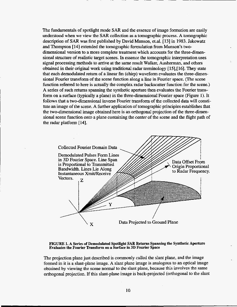
The fundamentals of spotlight mode S A R and the essence of image formation are easily understood when we view the SAR collection as a tomographic process. A tomographic description of S A R was first published by David Munson, et.al. [ 131 in 1983. Jakowatz and Thompson [ 141 extended the tomographic formulation from Munson's two- dimensional version to a more complete treatment which accounts for the three-dimensional structure of realistic target scenes. In essence the tomographic interpretation uses signal processing methods to arrive at the same result Walker, Ausherman, and others obtained in their original work using traditional radar terminology [ 15],[ 161. They state that each demodulated return of a linear fm (chirp) waveform evaluates the three-dimensional Fourier transform of the scene function along a line in Fourier space. (The scene function referred to here is actually the complex radar backscatter function for the scene.) A series of such returns spanning the synthetic aperture then evaluates the Fourier transform on a surface (typically a plane) in the three-dimensional Fourier space (Figure 1). It follows that a two-dimensional inverse Fourier transform of the collected data will constitute an image of the scene. A further application of tomographic principles establishes that the two-dimensional image obtained here is an orthogonal projection of the three-dimensional scene function onto a plane containing the center of the scene and the flight path of the radar platform [ 141.

\ Collected Fourier Domain Data Demodulated Pulses Form Lines

in is Proportional 3D Fourier Space. to T r a n s m i t t 2 6 Line Span Bandwidth. Lines Lie Along Instantaneous Xmitmeceive Vectors.

Data Origin Offset Proportional Frdm to Radar Frequency.

Data Projected to Ground Plane \ x

FIGURE 1. A Series of Demodulated Spotlight SAR Returns Spanning the Synthetic Aperture Evaluates the Fourier 'Ikansform on a Surface in 3D Fourier Space

The projection plane just described is commonly called the slant plane, and the image formed in it is a slant-plane image. A slant plane image is analogous to an optical image obtained by viewing the scene normal to the slant plane, because this involves the same orthogonal projection. If this slant-plane image is back-projected (orthogonal to the slant

10

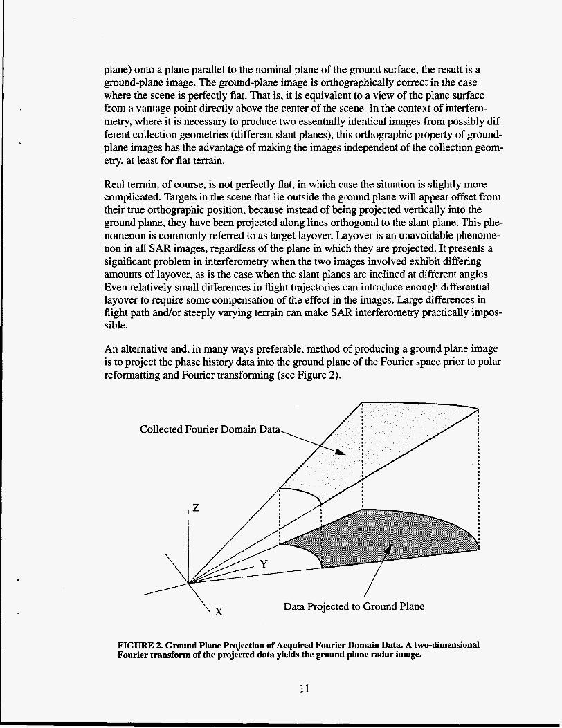
plane) onto a plane parallel to the nominal plane of the ground surface, the result is a ground-plane image. The ground-plane image is orthographically correct in the case where the scene is perfectly flat. That is, it is equivalent to a view of the plane surface from a vantage point directly above the center of the scene. In the context of interferometry, where it is necessary to produce two essentially identical images from possibly different collection geometries (different slant planes), this orthographic property of ground- plane images has the advantage of making the images independent of the collection geometry, at least for flat terrain.

Real terrain, of course, is not perfectly flat, in which case the situation is slightly more complicated. Targets in the scene that lie outside the ground plane will appear offset from their true orthographic position, because instead of being projected vertically into the ground plane, they have been projected along lines orthogonal to the slant plane. This phenomenon is commonly referred to as target layover. Layover is an unavoidable phenomenon in all S A R images, regardless of the plane in which they are projected. It presents a significant problem in interferometry when the two images involved exhibit differing amounts of layover, as is the case when the slant planes are inclined at different angles. Even relatively small differences in flight trajectories can introduce enough differential layover to require some compensation of the effect in the images. Large differences in flight path and/or steeply varying terrain can make SAR interferometry practically impos- sible.

An alternative and, in many ways preferable, method of producing a ground plane image is to project the phase history data into the ground plane of the Fourier space prior to polar reformatting and Fourier transforming (see Figure 2).

Collected F Collected Fourier Domain Data

\ / \ /

'ourier Domain Data

/ Data Projected to Ground Plane

FIGURE 2. Ground Plane Projection of Acquired Fourier Domain Data. A two-dimensional Fourier transform of the projected data yields the ground plane radar image.

11

To see that this procedure yields the same orthographic view of a scene as the image domain projection described above, it is necessary only to observe that a perfectly flat scene will exhibit no variation in the vertical dimension of the Fourier space in which the data were collected. In this case the data sampled in the slant plane are identical to data that would have been obtained by sampling directly in the ground plane of the Fourier domain. A slice of Fourier space in, or parallel to, the ground plane will produce an orthographic image by the projection arguments already given. The layover effect in this method of forming a ground plane image can be attributed to the fact that targets lying outside the ground plane of the scene will exhibit some variation in the vertical dimension of Fourier space. This variation is transduced into the data to the extent that the region of the slant plane spanned by the data covers some vertical distance. This in turn will be manifested in the image as an offset in position proportional to target height, which consti- tutes layover.

2.2 Coherent Pair Processing

Conventional S A R imaging emphasizes the magnitude of the formed image and generally ignores the phase, even though the image formation product is actually a complex valued map. Coherent pair processing for interferometry, by contrast, utilizes both magnitude and phase of the complex valued image. Since a coherent radar preserves the phase of the return signal, the Fourier space sampled in the S A R collection is the Fourier transform of the complex valued radar backscatter function for the terrain. Furthermore, because the polar reformatting and Fourier transformation involved in our image formation are linear operations, the formed image is a phase-preserving coherent image of the complex terrain backscatter function. The preservation of phase during the image formation process is essential to making SAR interferometry possible. Image formation processors that do not maintain phase integrity in this way are not compatible with coherent image processing.

A fundamental requirement for two SAR images to comprise a coherent pair suitable of interferometry is that they must have been collected with closely matched azimuth and grazing angles. A more precise statement of this requirement is that the Fourier-domain data collection regions for the two images, when projected into the ground plane, must significantly overlap one another. To see that this is the case, consider first a pair of coherent images that have been formed using identical collection geometries. In this case both collections involve sampling the same region of the Fourier space, so the two complex images will be identical in both magnitude and phase, and they may be thought of as “completely coherent.” Now imagine that the two collection geometries differ somewhat, so that the ground plane projections of the two phase history regions are offset, but still partially overlapping. It is a property of Fourier transform theory that a translation in one domain introduces a linear phase shift in the transform domain. Thus, if a pair of SAR phase histories are relatively offset, the corresponding images will differ by a linear phase ramp in a certain direction. If the slope of this phase ramp is small, corresponding, say, to several cycles of phase difference across the scene, the images will remain essentially coherent in local regions. But as the slope of the differential phase ramp increases, the regions of local coherence will shrink and finally vanish completely as the phase gradient approaches a full cycle per pixel. One cycle of phase shift per pixel would correspond to a relative phase history offset equal to the width of the aperture, i.e., the point at which the

12

phase histories no longer contain any overlapping region. We conclude that successful interferometry of a pair of images will require their respective phase histories (in ground plane projection) to significantly overlap one another.

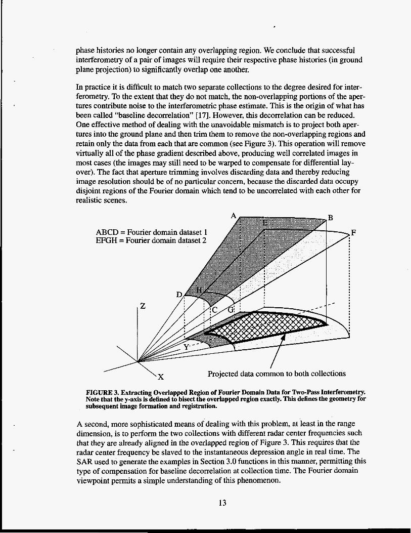
In practice it is difficult to match two separate collections to the degree desired for interferometry. To the extent that they do not match, the non-overlapping portions of the aper- tures contribute noise to the interferometric phase estimate. This is the origin of what has been called “baseline decorrelation” [ 171. However, this decorrelation can be reduced. One effective method of dealing with the unavoidable mismatch is to project both aper- tures into the ground plane and then him them to remove the non-overlapping regions and retain only the data from each that are common (see Figure 3). This operation will remove virtually all of the phase gradient described above, producing well correlated images in most cases (the images may still need to be warped to compensate for differential layover). The fact that aperture trimming involves discarding data and thereby reducing image resolution should be of no particular concern, because the discarded data occupy disjoint regions of the Fourier domain which tend to be uncorrelated with each other for realistic scenes.

ABCD = Fourier domain dataset 1 EFGH = Fourier domain dataset 2 ,

F

w

/ Projected data common to both collections

FIGURE 3. Extracting Overlapped Region of Fourier Domain Data for Wo-Pass Interferometry. Note that the y-axis is defined to bisect the overlapped region exactly. This defines the geometry for subsequent image formation and registration.

A second, more sophisticated means of dealing with this problem, at least in the range dimension, is to perform the two collections with different radar center frequencies such that they are already aligned in the overlapped region of Figure 3. This requires that the radar center frequency be slaved to the instantaneous depression angle in real time. The S A R used to generate the examples in Section 3.0 functions in this manner, permitting this type of compensation for baseline decorrelation at collection time. The Fourier domain viewpoint permits a simple understanding of this phenomenon.

13

2.3 ComDlex Image Registration

S A R interferometry is based on obtaining the difference in phase of the complex reflectivity of two images. This requires that the two images be precisely registered, as the complex reflectivity of natural terrain is essentially delta correlated [18]. Thus, entire images need to be registered to a fraction of the main lobe of an impulse response function. For single pass, displaced phase center systems, this is not a burdensome requirement, especially at low spatial resolutions. However, two-pass, high resolution SAFt interferometry demands data driven automatic registration of the image pairs. Platform position and imaging geometry errors introduce misregistrations that are considerable compared to image resolution. Large track crossing angles further compound this problem. In this Sec- tion, we explore the issues and techniques of complex image registration.

2.3.1 Introduction to Registration. Image registration techniques developed for low- resolution strip map SARs [19][20], and for small track crossing angles [21], are inadequate for this task and computationally inefficient. In this section we develop a robust, efficient, and automatic registration procedure applicable to a wide range of high resolution, two-pass, parallel or non-parallel ground track interferometric collections.

Data driven image registration techniques abound in the literature [22]. Generally, these techniques make local measurements of image-to-image displacement, called control points, at many locations. One image is then warped or resampled to overlay the second. The control point measurements can be made using projection properties [23], feature identification [24], or correlation. Variations include multiresolution, recursive, and iterative methods. For this application, the authors use a multiresolution, correlation based technique. Because of differential layover effects (discussed below), high resolution two- pass interferometric image pairs cannot always be registered by global transformations. This necessitates a dense set of control points. Substantial translation and rotation between the pair of images may also be present, which argues for a multiresolution approach. The method of obtaining control point information described in [21] is effective but computationally expensive. In that reference, the data are shifted, conjugate multiplied, and trans- formed to ascertain the presence of a fringe spectrum. A conjugate multiply and a 2D transform is required for every shift value. It is much more efficient to obtain the cross correlation function through the use of fast transform methods. Since interferometric image pairs are coherent, the complex data have a much more pronounced autocorrelation peak than the magnitude only data. A potential problem with this method would result from the presence of phase ramps in one image relative to the other. A two dimensional relative phase ramp between the two images is indicative of an offset between their corresponding spatial frequency domain data. Thus, it is imperative to avoid such an offset by processing into imagery that phase history data lying in the overlapped region of spatial frequencies, as described in Section 2.2. If the imagery is not processed from phase histories in this fashion, it is possible to estimate and remove the dominant image domain fringe frequency. This situation will not be considered further here.

14

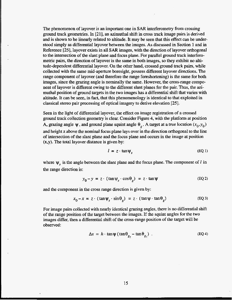
The phenomenon of layover is an important one in SAR interferometry from crossing ground track geometries. In [21], an azimuthal shift in cross track image pairs is derived and is shown to be linearly related to altitude. It may be seen that this effect can be understood simply as differential layover between the images. As discussed in Section 1 and in Reference [25], layover exists in all SAR images, with the direction of layover orthogonal to the intersection of the slant plane and focus plane. For parallel ground track interferometric pairs, the direction of layover is the same in both images, so they exhibit no altitude-dependent differential layover. On the other hand, crossed ground track pairs, while collected with the same mid-aperture boresight, possess different layover directions. The range component of layover (and therefore the range foreshortening) is the same for both images, since the grazing angle is nominally the same. However, the cross-range component of layover is different owing to the different slant planes for the pair. Thus, the azimuthal position of ground targets in the two images has a differential shift that varies with altitude. It can be seen, in fact, that this phenomenology is identical to that exploited in classical stereo pair processing of optical imagery to derive elevation [25].

Seen in the light of differential layover, the effect on image registration of a crossed ground track collection geometry is clear. Consider Figure 4, with the platform at position A, grazing angle v , and ground plane squint angle 8,. A target at a true location (xo ,yo) and height z above the nominal focus plane lays over in the direction orthogonal to the line of intersection of the slant plane and the focus plane and occurs in the image at position (x,y). The total layover distance is given by:

where v, is the angle between the slant plane and the focus plane. The component of I in the range direction is:

and the component in the cross range direction is given by:

For image pairs collected with nearly identical grazing angles, there is no differential shift of the range position of the target between the images. If the squint angles for the two images differ, then a differential shift of the cross-range position of the target will be observed:

hx = h - tanv(tanegZ- tan€),,) . (EQ 4)

15

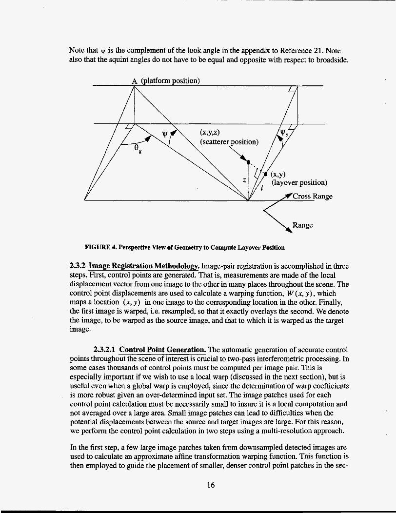
Note that w is the complement of the look angle in the appendix to Reference 21. Note also that the squint angles do not have to be equal and opposite with respect to broadside.

A (platform position)

(layover position)

/Cross Range

\Range

FIGURE 4. Perspective View of Geometry to Compute Layover Position

2.3.2 Image Registration Methodology. Image-pair registration is accomplished in three steps. First, control points are generated. That is, measurements are made of the local displacement vector from one image to the other in many places throughout the scene. The control point displacements are used to calculate a warping function, W (x, y ) , which maps a location (x, y) in one image to the corresponding location in the other. Finally, the first image is warped, i.e. resampled, so that it exactly overlays the second. We denote the image, to be warped as the source image, and that to which it is warped as the target image.

2.3.2.1 Control Point Generation. The automatic generation of accurate control points throughout the scene of interest is crucial to two-pass interferometric processing. In some cases thousands of control points must be computed per image pair. This is especially important if we wish to use a local warp (discussed in the next section), but is useful even when a global warp is employed, since the determination of warp coefficients is more robust given an over-determined input set. The image patches used for each control point calculation must be necessarily small to insure it is a local computation and not averaged over a large area. Small image patches can lead to difficulties when the potential displacements between the source and target images are large. For this reason, we perform the control point calculation in two steps using a multi-resolution approach.

In the first step, a few large image patches taken from downsampled detected images are used to calculate an approximate affine transformation warping function. This function is then employed to guide the placement of smaller, denser control point patches in the sec-

16

ond step. If we denote the data from one image patch as If( i, j ) 1, the data from the second image as [ g (i, j) 1, and their corresponding 2D Fourier transform pairs as [ F (my n) 1, and [ G (my n) 1, then we form:

where !T1 denotes an inverse 2D Fourier transform. The cross correlation function [ r (i, j ) ] contains a sharp peak whose offset from the origin is a measure of the local displacement vector from f to g . The precise location of the correlation peak is obtained by a quadratic interpolation of the four nearest sample points. Since the image data is pos- itive (magnitude), the dc term F (0,O) G* (0,O) is set to zero before the inverse transform is taken to remove the bias. Poor control points may result from a variety of conditions. The image patches might fall in a portion of the SAR image that is in radar shadow, over water, in a region of temporal change, etc. Poor control points are edited by establishing a threshold on the peak-to-variance ratio of the cross correlation function.

Having determined an approximate affine transformation from the source image to the target image, we proceed to the second, high resolution control point step. The source image need not be warped at this time. Rather, the affine transform is used to calculate the position of image patches in the source image that roughly correspond to the position of similar patches in the target image. Control points are then calculated using full resolution complex data in the correlator. Since complex data are correlated in this step, two modifi- cations of (EQ 5) are necessary. The dc term does not have to be zeroed, as complex image data has no appreciable dc component. Also we must accommodate variations in the local terrain slope. Sloping terrain introduces a relative phase gradient across the patch from one image to the other. We therefore form the Fourier transform of the image domain data as before, but evaluate a number of cross correlation arrays:

and choose that [I ( i, j ) ] (k, E) with the largest peak-to-variance ratio. Since any large phase gradient has been avoided by forming imagery from the overlapped portion of the phase history data (see Section 2.2), small values of the search parameter p (0 or 1) may be employed. As before, the set of high resolution control points is edited to remove those with a poor peak-to-variance ratio.

A final consideration arises from differential layover in the case of crossed ground track geometries. After taking into account the affine transformation measured by the low resolution step, the cross range shift given by (EQ 4) may result in height induced local displacements which exceed the high resolution image patch size. In this case, we must either use larger image patches or correlate several image patches of the target image, displaced in the cross range direction, with the source image patch. The latter is more efficient since we are confining the additional search space to one direction (cross range).

17

2.3.2.2 Image Warping. After a dense set of accurate control points is obtained by the procedure described above, the source image must be resampled. We may proceed in one of two ways. We may perform a global warp based on a 2D polynomial fit to the control point displacements, or we may perform a local warp. As discussed Section 2.3.1, if parallel ground track collection geometries are employed, there is no differential layover induced misregistration present no matter what the terrain relief. However, crossing ground track collection geometries, in the presence of terrain relief, introduce cross range positional shifts due to differential layover. Thus, a global polynomial warp may be used when: a) the ground track angles differ only slightly (parallel collections), and/or b) the terrain relief is small, and/or c) the images are small. Otherwise, a local warp must be employed to accommodate the terrain-induced displacements.

A global polynomial warping function W (x, y ) is determined by linear regression. A least squares solution to an overdetermined system of linear equations AX = B is obtained by conventional methods. The authors employ a second order 2D polynomial for global warps. Once the polynomial W is determined, the source image is resampled using a bilinear interpolator to register it with the target image.

Local warps are somewhat more complicated. We combine both a polynomial and a spline warp in this processing step. A first order 2D polynomial (affine transformation) is first determined as above. This is done principally to accommodate image rotation, since spline function surface fitting is ill suited to that task. Beyond the affine transformation, any residual misregistration results from the differential layover in the cross range direction given by (EQ 4). This residual, which varies across the image as a function of terrain height, can be accommodated by a surface fitting technique. We use a triangular mesh spline fitting method. The processing proceeds as follows. An affine transformation A ( x , y ) is calculated from the control point displacements by linear regression. For each control point, the displacement predicted by the affine transformation is subtracted from the actual displacement:

where D ( x , y ) is the control point displacement at (x, y ) . The residual displacements are then fit by the surface fitting routine to obtain a surface function, S ( x , y ) . Note that this function S is a scaled approximation to the terrain relief. The final warping function is therefore equal to the sum of the affine transformation and the surface fit:

With the warping function in hand, the source image can then be resampled to overlay the target image.

18

2.4 Spatial Correlation and Interferometric Change Detection

After the pair of complex images are appropriately registered, we may form the interferometric products. The registered images may be combined to yield: a) a “change” map, and b) a phase difference map. The change map is a two dimensional image showing where the complex reflectivity of the terrain has either remained the same or been altered between the image collections. This product is only applicable to two-pass collections. As will be shown later in Section 3.3, this technique is extraordinarily sensitive to physical disturbances, as compared to non-coherent change detection, since the phase of a distrib- uted reflector such as the ground is easily perturbed. We may also calculate a phase difference map in those portions of the image pair that have not undergone temporal changes. Where the images do not correlate, the phase difference values will be random on the interval [ -.n‘,n: 1. However, if they do correlate, the spatial pattern of wrapped phase differences gives rise to the interference fringe patterns typical of these datasets. Furthermore, these values contain the highly accurate path length difference information which allows post-processing techniques to measure terrain elevation with extraordinary accuracy as we shall later demonstrate.

We now show the derivation of an optimal estimate of the phase difference map obtained from the two complex input images used for the INSAR processing. This in turn provides the input for the phase unwrapping algorithm, from which terrain elevation maps are ultimately computed. We denote the measured complex reflectivity at pixel k from the first and second collections as g, and h, respectively. These measured values are represented by the model:

where Sk denotes the true scene reflectivity, n l , and n2, , are the additive measurement noise terms, and Q is a phase rotation induced by the terrain elevation. It is Q that we wish to estimate. The random variables s,, n l , ,, n2, k , and zk are all assumed to be zero-mean, Gaussian, and mutually independent with the following statistics:

E { $ } = E{zZ} = 0,’

e 0,’ *

In addition, the signal-to-noise ratio of the process is defined as SNR = -

19

At this point it is convenient to define the observation for pixel k in vector form as:

Using the above statistical assumptions, one can easily write the conditional probability density function (PDF) of conditioned on the parameters Q and a as:

1 P ( 2 k / @ ) = -eXp {-kHkQ-lkk}, . ~ c ~ l Q l

where the superscript H denotes the complex-conjugate transpose and

In reality, we assume there exists a neighborhood of N pixels, all of Nc.,ich have "een rotated by the same phase angle Q . These pixels are treated as independent observations, since the noise is uncorrelated from sample to sample, which allows the conditional PDF of all observations to be written as the product of the individual PDFs. The resulting conditional PDF is then:

where fi denotes a vector containing all N complex observations.

The ML estimate of Q will be denoted as $ml and is that value of Q that maximizes (EQ 48) or equivalently the logarithm of (EQ 48). The logarithm is given by:

Note that the term I Ql is not a function of Q , because:

20

As a result, the solution for 6ml can be obtained by maximizing the second term of (EQ 15). It is easily shown that this is equivalent to maximizing:

Inspection of (EQ 17) reveals that the solution for f ~ ~ l is:

In order to obtain a map to depict changes that occurred between pre- and post-collections, we compute the sample complex spatial correlation coefficient over a sliding local window:

I N I

k = 1 k = l

We show in the Appendix that eml is a maximum likelihood estimate of the change. Fur- thermore, this statistic may be computed recursively, with an execution time that is independent of the window size. The choice of the sample sti‘ stic window size is a function of the radar clutter-to-system noise ratio and spatial resolution desired. For the examples presented in Section 3.0, a window size of 5 x 5 was used.

2.5 2D Phase Unwrapping

Two-dimensional phase unwrapping is the final major computational step required in forming the terrain elevation estimate. Computation of the phase values from the argument of the complex correlation coefficient yields wrapped values. That is, all wrapped phase samples lie between +n: radians. These phase values must be unwrapped over a 2D grid and then scaled to represent an estimate of the true terrain elevation.

21

The mathematical formalism for reconstructing a 2D phase surface from noisy phase difference measurements had its roots in adaptive optics and speckle imaging, Since the phase differences were usually obtained in two orthogonal directions (i.e., x and y) from wave-front tilt sensors, the problem was to reconstruct the phase, in a least-squares sense, from those noisy measurements. The papers by Fried [26], Hudgin [27], No11 [28], and Hunt [29], provide a thorough background.

Recent research has shown that the least-squares solution to the phase unwrapping problem is mathematically identical to the solution of Poisson’s equation on a rectangular grid with Neumann boundary conditions [30],[3 11. SAR interferometry for terrain elevation mapping forces the requirement for phase unwrapping on very large grids (i.e.,up to O(16K by 16K)), efficient use of available memory, and 32-bit precision, as is commonly available on modern workstations. All the above requirements can be met, without numer- ical difficulty, by solving Poisson’s equation using a specific form of the fast cosine transform [32]. This approach is numerically stable and robust, exactly solves Poisson’s equation, automatically imposes the proper boundary conditions, can be posed as a separa- ’ble process (computationally efficient), can be performed “in place” with regard to available memory, and does not require any cumbersome “path-following” logic or heuristics [33]. This new unweighted 2D phase unwrapping algorithm, originally presented in [32], will be summarized below. Weighted 2D phase unwrapping, which can elegantly solve problems containing phase dislocations andor arbitrary region partitioning will not be presented here. The reader is encouraged to consult [32] for a thorough treatment.

2.5.1 2D Unweighted Least-Squares Phase Unwrapping. Let us assume that we know the phase, @ modulo 2n, of a function on a discrete grid of points:

W i , j = @i,j + 2nk, k an integer, (EQ 20)

-n<lyii jIn, i = O...M-1, j = O...N-1.

Given the wrapped phase values yj, , we wish to determine the unwrapped phase values $ i , j , at the same grid locations with the requirement that the phase differences of the @i,

agree with those of the vi, in the least-squares sense. To see how this is done, let us first define a wrapping operator W , that wraps all values of its argument into the range (-n, n) by adding or subtracting an integral number of 2n radians from its argument.

Therefore, for example, W { @i, j } = vi, j .

Next, we compute two sets of phase differences: those differences with respect to the i index, and those with respect to the j index. Specifically, from our known values of the wrapped phase vi, , we compute the following wrapped phase differences,

22

i = O...M-2, j = O . . . N - 1

A t j = 0 , otherwise,

and,

Ai: j = W {Vi, j + 1 - Vi, j l

i = O . . . M - 1 , j = O . . . N - 2

A[ j = 0 , otherwise,

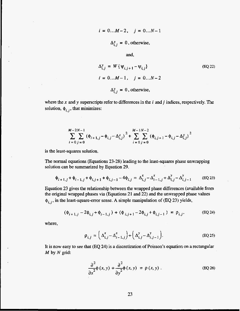
where the x and y superscripts refer to differences in the i and j indices, respectively. The solution, @i, j , that minimizes:

is the least-squares solution.

The normal equations (Equations 23-28) leading to the least-squares phase unwrapping solution can be summarized by Equation 29.

Equation 23 gives the relationship between the wrapped phase differences (available from the original wrapped phases via (Equations 21 and 22) and the unwrapped phase values $i, j 9 in the least-square-error sense. A simple manipulation of (EQ 23) yields,

where,

Pi , j = [A; - AT- 1 , j ) + [A: - A: j - J.

It is now easy to see that (EQ 24) is a discretization of Poisson’s equation on a rectangular M by N grid:

23

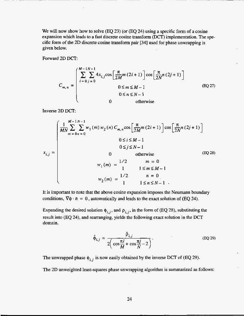
We will now show how to solve (EQ 23) (or (EQ 24) using a specific form of a cosine expansion which leads to a fast discrete cosine transform (DCT) implementation. The specific form of the 2D discrete cosine transform pair [34] used for phase unwrapping is given below.

Forward 2D DCT

Inverse 2D DCT

0

OlmSM-1 0 5 n I N - 1

otherwise

M - 1 N - 1

- 1 c c wl(m)w2(n)~m,ncos[~m(2i+l)]cos[~n(2j+ n: 111

m = O n = O MN

(EQ 27)

O S i l M - 1 OIj5N-1

0 otherwise 1 /2 m = O

1 1 I m S M - 1 w1(m> =

n = O 15nlN-1 -

It is important to note that the above cosine expansion imposes the Neumann boundary conditions, V$ R = 0 , automatically and leads to the exact solution of (EQ 24).

Expanding the desired solution $i, j , and pi, , in the form of (EQ 28), substituting the result into (EQ 24), and rearranging, yields the following exact solution in the DCT domain.

The unwrapped phase Oj, is now easily obtained by the inverse DCT of (EQ 29).

The 2D unweighted least-squares phase unwrapping algorithm is summarized as follows:

24

1. Perform the 2D forward DCT (EQ 27) of the array of values, pi, j , computed by (EQ

2. Modify the values according to (EQ 29) to obtain $ i , j .

3. Perform the 2D inverse DCT (EQ 28) of $ i , j to obtain the least-squares unwrapped phase values + c j .

25), to yield the 2D DCT values pi, j .

2.5.2 Phase Distortion Correction from Wavefront Curvature. In general, because of wavefront curvature, there is a global phase distortion imposed on the interferometric phase data that must be removed prior to phase unwrapping. If not removed, the unwrapped phase will be an inaccurate representation of the underlying terrain. For example, the phase distortion is more severe (for a given patch diameter) when imaging at short ranges (as compared to long ranges) because of the wavefront curvature.

Recall that the interferometric phase (to be unwrapped) is derived as the phase of the complex spatial correlation coefficient. This phase is the result of a moving window spatial average of a complex function whose argument is the &Terence of phases of the underlying complex imagery. Because of wavefront curvature the phase resulting from imaging perfectly flat terrain will not be strictly planar.

Whether it be a two-antenna or two-pass interferometry collection, SAR spotlight collection and processing allows simple descriptions for image collections, phase history domain geometry, and differential layover effects. With reference to Figure 5, we can assume that two spotlight images were collected from two slightly different vantage points. Images 1 and 2 were collected with the SAR platform at (effectively) points (xl, y l , zl) and (x2, y2, z2) , respectively, whereas a scatterer is located at the point (x, y , z ) . The slant ranges from each vantage point to the scatterer is represented as:

1

The differential phase (between images 1 and 2) for a scatterer at height z is given by:

where h is the nominal radar wavelength in the desired units.

The phase distortion (in x and y) results from the non-planar component of (EQ 31) when z = 0 in (EQ 30). This phase distortion function will be designated as cp (x, y ) and can be computed directly from (EQ 3 1) as x and y cover the image space over the allowable range of values. Once cp (x, y ) is computed, it is removed from the second image in the

25

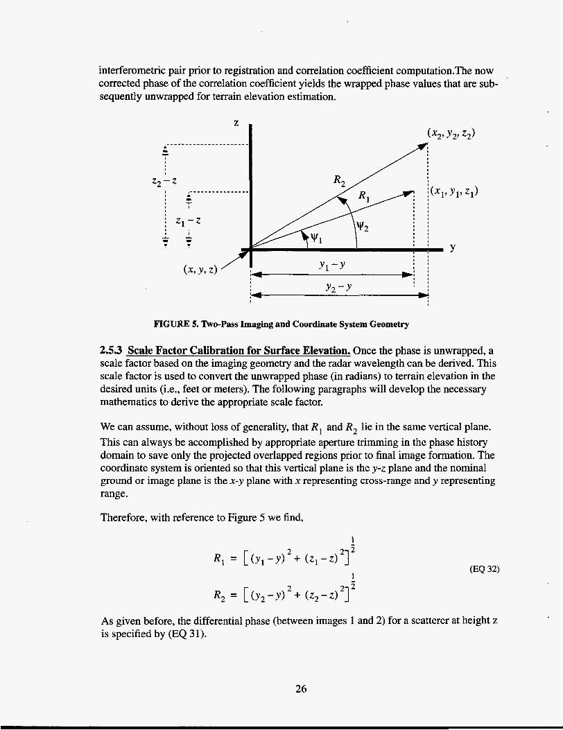
interferometric pair prior to registration and correlation coefficient computation.The now corrected phase of the correlation coefficient yields the wrapped phase values that are sub- sequently unwrapped for terrain elevation estimation.

FIGURE 5. Two-Pass Imaging and Coordinate System Geometry

2.5.3 Scale Factor Calibration for Surface Elevation. Once the phase is unwrapped, a scale factor based on the imaging geometry and the radar wavelength can be derived. This scale factor is used to convert the unwrapped phase (in radians) to terrain elevation in the desired units (i.e., feet or meters). The following paragraphs will develop the necessary mathematics to derive the appropriate scale factor.

We can assume, without loss of generality, that R , and R, lie in the same vertical plane. This can always be accomplished by appropriate aperture trimming in the phase history domain to save only the projected overlapped regions prior to final image formation. The coordinate system is oriented so that this vertical plane is the y-z plane and the nominal ground or image plane is the x-y plane with x representing cross-range and y representing range.

Therefore, with reference to Figure 5 we find,

1

As given before, the differential phase (between images 1 and 2) for a scatterer at height z is specified by (EQ 31).

26

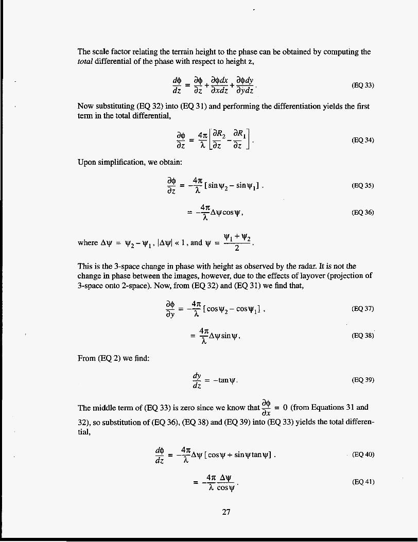
The scale factor relating the terrain height to the phase can be obtained by computing the total differential of the phase with respect to height z,

(EQ 33)

Now substituting (EQ 32) into (EQ 31) and performing the differentiation yields the first term in the total differential,

Upon simplification, we obtain:

9 = -@ [sinv2 - sinvl] . az h

VI + w 2 2 where Ay = y2- yl, IAyI << 1 , and v =

This is the 3-space change in phase with height as observed by the radar. It is not the change in phase between the images, however, due to the effects of layover (projection of 3-space onto 2-space). Now, from (EQ 32) and (EQ 31) we find that,

4n 3 = -- [cosy2- cosy1] , aY h

= g A y s i n y , h

(EQ 37)

(EQ 38)

From (EQ 2) we find:

(EQ 39) dY - = -tan\y. dz

a+ ax The middle term of (EQ 33) is zero since we know that - = 0 (from Equations 31 and

32), so substitution of (EQ 36), (EQ 38) and (EQ 39) into (EQ 33) yields the total differential,

4n h '+ - --AV [cosv + sinvtanv] .

dz - - (EQ 40)

- 4n A y - --- h cosy .

27

Finally, the scale factor relating height to total phase shift is given by:

The unwrapped phase surface is multiplied by the above scale factor to obtain the terrain elevation in the appropriate units. In addition, any residual planar component is removed by tying three non-colinear points to actual surveyed elevations. The final elevation map is accurate relative to these surveyed points and to within the limits imposed by phase noise and phase aliasing from overly steep terrain relative to the interferometric baseline.

3.0 Examples In this section, we step through the processing required to produce an interferometric terrain elevation map. The imagery for these examples was acquired with the SAR test bed system. This radar flies aboard a DHC-6-300 “Twin-Otter” aircraft. The imagery is collected in a spotlight mode with a nominal resolution of 1 meter. A significant feature of this system is the navigation equipment available. The navigator uses a high precision and miniaturized ring laser gyro inertial measurement unit tightly coupled to differential GPS. This allows the collection geometry to be controlled and known to a high degree of accuracy. The navigator is described in some detail in Reference 35.

3.1 Terrain Elevation Mapping

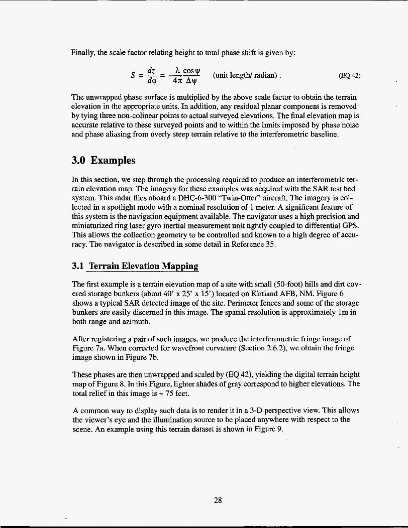
The first example is a terrain elevation map of a site with small (50-foot) hills and dirt cov- ered storage bunkers (about 40’ x 25’ x 15,) located on Kirtland AFB, NM. Figure 6 shows a typical SAR detected image of the site. Perimeter fences and some of the storage bunkers are easily discerned in this image. The spatial resolution is approximately lm in both range and azimuth.

After registering a pair of such images, we produce the interferometric fringe image of Figure 7a. When corrected for wavefront curvature (Section 2.6.2), we obtain the fringe image shown in Figure 7b.

These phases are then unwrapped and scaled by (EQ 42), yielding the digital terrain height map of Figure 8. In this Figure, lighter shades of gray correspond to higher elevations. The total relief in this image is - 75 feet.

A common way to display such data is to render it in a 3-D perspective view. This allows the viewer’s eye and the illumination source to be placed anywhere with respect to the scene. An example using this terrain dataset is shown in Figure 9.

28

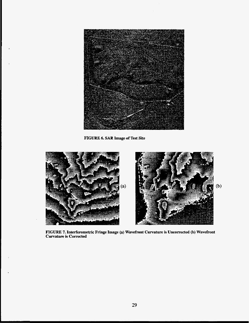
FIGURE 7. Interferometric Fringe Image (a) Wavefront Curvature is Uncorrected (b) Wavefront Curvature is Corrected

29

FIGURE 8. Digital Terrain Elevation Map

FIGURE 9. Perspective View of Digital Terrain Elevation Data (DTED) Map

Many small features are quite evident in this Figure. For example, where the perimeter fence is seen in Figure 6, it is also noticeable in Figure 9 as an elevated feature. The storage bunkers are also easily discernible.

Finally, in Figure 10, we show a contour map derived from DTED data next to a contour map generated by a commercial surveying company using optical stereoscopy techniques (at very low altitudes). The contour interval is two feet.

30

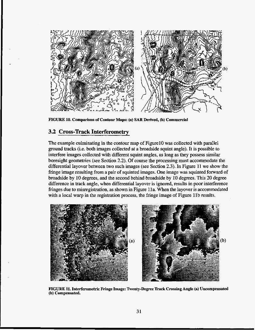
FIGURE 10. Comparison of Contour Maps: (a) SAR Derived, (b) Commercial

3.2 Cross-Track Interferometw

The example culminating in the contour map of Figure10 was collected with parallel ground tracks (Le. both images collected at a broadside squint angle). It is possible to interfere images collected with different squint angles, as long as they possess similar boresight geometries (see Section 2.2). Of course the processing must accommodate the differential layover between two such images (see Section 2.3). In Figure 11 we show the fringe image resulting from a pair of squinted images. One image was squinted forward of broadside by 10 degrees, and the second behind broadside by 10 degrees. This 20 degree difference in track angle, when differential layover is ignored, results in poor interference fringes due to misregistration, as shown in Figure 1 la. When the layover is accommodated with a local warp in the registration process, the fringe image of Figure l l b results.

FIGURE 11. Interferometric Fringe Image: Twenty-Degree Track Crossing Angle (a) Uncompensated (b) Compensated.

31

3.3 Interferometric Change Detection

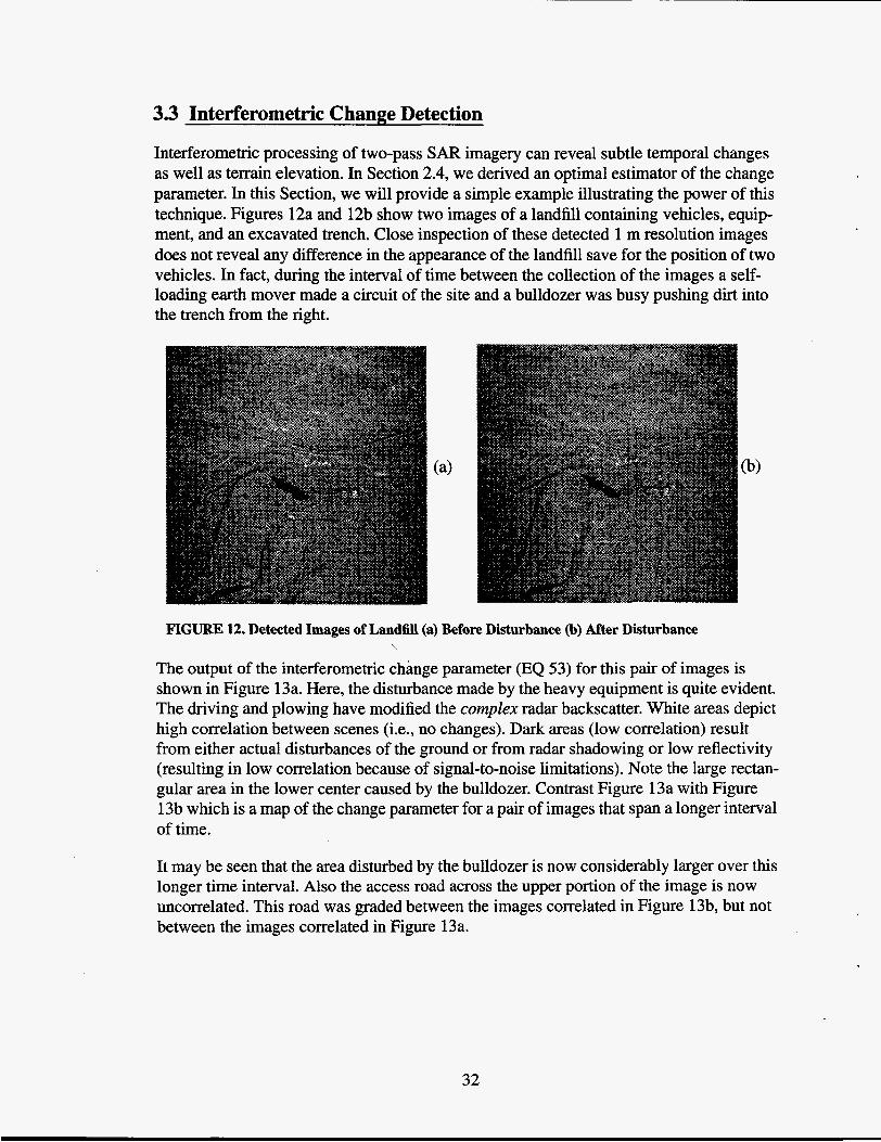
Interferometric processing of two-pass SAR imagery can reveal subtle temporal changes as well as terrain elevation. In Section 2.4, we derived an optimal estimator of the change parameter. In this Section, we will provide a simple example illustrating the power of this technique. Figures 12a and 12b show two images of a landfill containing vehicles, equipment, and an excavated trench. Close inspection of these detected 1 m resolution images does not reveal any difference in the appearance of the landfill save for the position of two vehicles. In fact, during the interval of time between the collection of the images a self- loading earth mover made a circuit of the site and a bulldozer was busy pushing dirt into the trench from the right.

FIGURE 12. Detected Images of Landfill (a) Before Disturbance (b) After Disturbance

The output of the interferometric change parameter (EQ 53) for this pair of images is shown in Figure 13a. Here, the disturbance made by the heavy equipment is quite evident. The driving and plowing have modified the compEex radar backscatter. White areas depict high correlation between scenes (i.e., no changes). Dark areas (low correlation) result from either actual disturbances of the ground or from radar shadowing or low reflectivity (resulting in low correlation because of signal-to-noise limitations). Note the large rectangular area in the lower center caused by the bulldozer. Contrast Figure 13a with Figure 13b which is a map of the change parameter for a pair of images that span a longer interval of time.

It may be seen that the area disturbed by the bulldozer is now considerably larger over this longer time interval. Also the access road across the upper portion of the image is now uncorrelated. This road was graded between the images correlated in Figure 13b, but not between the images correlated in Figure 13a.

32

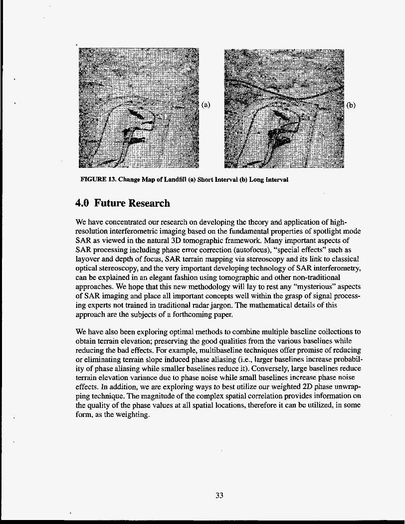
FIGURE 13. Change Map of Landfill (a) Short Interval (b) Long Interval

4.0 Future Research We have concentrated our research on developing the theory and application of high- resolution interferometric imaging based on the fundamental properties of spotlight mode S A R as viewed in the natural 3D tomographic framework. Many important aspects of S A R processing including phase error correction (autofocus), “special effects” such as layover and depth of focus, SAR terrain mapping via stereoscopy and its link to classical optical stereoscopy, and the very important developing technology of SAR interferometry, can be explained in an elegant fashion using tomographic and other non-traditional approaches. We hope that this new methodology will lay to rest any “mysterious” aspects of SAR imaging and place all important concepts well within the grasp of signal processing experts not trained in traditional radar jargon. The mathematical details of this approach are the subjects of a forthcoming paper.

We have also been exploring optimal methods to combine multiple baseline collections to obtain terrain elevation; preserving the good qualities from the various baselines while reducing the bad effects. For example, multibaseline techniques offer promise of reducing or eliminating terrain slope induced phase aliasing (i.e., larger baselines increase probability of phase aliasing while smaller baselines reduce it). Conversely, large baselines reduce terrain elevation variance due to phase noise while small baselines increase phase noise effects. In addition, we are exploring ways to best utilize our weighted 2D phase unwrapping technique. The magnitude of the complex spatial correlation provides information on the quality of the phase values at all spatial locations, therefore it can be utilized, in some form, as the weighting.

33

5.0 Conclusions We have developed much of the theory of interferometric S A R from a non-traditional viewpoint and delineated, in this paper, the required sequence of events, processing steps, and innovations resulting from that viewpoint. We have shown several practical examples of very accurate terrain elevation maps and subtle interferometric change detection results. The two-pass spotlight modality and 3D tomographic construct allowed exploration of the full range of interferometric possibilities and allowed derivation of the fundamental limitations and constraints imposed on practical S A R interferometry.

34

References [l] L. C. Graham, “Synthetic interferometer radar for topographic mapping,” Proc.

[2] H. A. Zebker, and R. M. Goldstein, “Topographic mapping from interfero- IEEE, Vol. 62, No. 6, pp. 763-768, June 1974.

metric synthetic aperture radar observations,” J. Geophysical Res., Vol. 91, No. B5, pp. 4993-4999, April 10,1986.

[3] E K. Li, and R. M. Goldstein, “Studies of multibaseline spaceborne interferometric synthetic aperture radars,” IEEE Trans. Geoscience and Remote Sensing, Vol. 28, NO. 1, pp. 88-97, January 1990.

[4] E. Rodriguez, and J. M. Martin, “Theory and design of interferometric synthetic aperture radars,” IEE Proceedings F, Vol. 139, No. 2, pp. 147-159, April 1992.

[SI A. L. Gray, and P. J. Farris-Manning, “Repeat-pass interferometry with air- borne synthetic aperture radar,” IEEE Trans. Geoscience and Remote Sensing, Vol. 3 1, NO. 1, pp. 180-191, January 1993.

f6] J. Villasenor, and H. A. Zebker, “Studies of temporal change using radar inter-

[7] A. K. Gabriel, R. M. Goldstein, and H. A. Zebker, “Mapping small elevation ferometry,” Synthetic Aperture Radar, SPIE Vol. 1630, pp. 187-198, (1992).

changes over large areas: Differential radar interferometry,” J. Geophysical Res., Vol. 94, NO. B7, pp. 9183-9191, July 10, 1989.

[SI D. Massonnet, M. Rossi, C. Carmona, F. Adragna, G. Peltzer, K. Feigl, and T. Rabaute, “The displacement field of the Landers earthquake mapped by radar interferometry,” Nature, Vol. 364, pp. 138-142, July 8, 1993.

S A R focusing: Interferometrical applications,” IEEE Trans. Geoscience and Remote Sensing, Vol. 28, No. 4, pp. 627-640, July 1990.

[lo] Q. Lin, J. E Vesecky, and H. A. Zebker, “New approaches in interferometric SAR data processing,” E E E Trans. Geoscience and Remote Sensing, Vol. 30, No. 3, pp. 560-567, May 1992.

interferometry: Processing techniques,” IEEE Trans. Geoscience and Remote Sensing,

[9] C. Prati, F. Rocca, A. M. Guamieri, and E. Damonti, “Seismic migration for

[ 113 S. N. Madsen, H. A. Zebker, and J. Martin, “Topographic mapping using radar

Vol. 31, NO. 1, pp. 246-256, Jan~ary 1993. [12] J. 0. Hagberg, and L. M. H. Ulander, “On the optimization of interferometric

SAR for topographic mapping,” IEEE Trans. Geoscience and Remote Sensing, Vol. 3 1 , NO. 1, pp. 303-306, January 1993.

[13] D. C. Munson, Jr., J.D. Obrien, K.W. Jenkins, “A tomographic formulation of

[ 141 C. V. Jakowatz and P. A. Thompson, “A new look at spotlight-mode synthetic spotlight-mode synthetic aperture radar,” IEEE Proc., 71, No. 8, pp. 917-925, (1983).

aperture radar as tomography: Imaging three-dimensional targets,” submitted to IEEE Trans. on Image Roc.

35

[15] D. A. Ausherman, A. Kozma, J. L. Walker, H. M. Jones, and E. C. Poggio, “Developments in radar imaging,” IEEE Transactions on Aerospace and Electronics Sys- tem, AES-20, No. 4, pp. 363-400, (1984).

[ 161 J. Walker, “Range-Doppler imaging of rotating objects,” EEE Transactions,

[ 171 H. A. Zebker, and J. Villasenor, “Decorrelation in interferometric radar echoes,” IEEE Trans. Geoscience and Remote Sensing, Vol. 30, No. 5, pp. 950-959, September 1992.

[18] J. W. Goodman, “Some fundamental properties of speckle,” J. Opt. SOC. Am., Vol. 66, No. 11, pp. 1145-1150, November 1976.

[19] J.C. Curlander, R. Kwok, and S.S. Pang, “A post-processing system for auto- mated rectification and registration of spaceborne SAR imagery,” International Journal of Remote Sensing, Vol. 8, No. 4, pp. 621-638, April 1987.

[20] C. Elachi, T. Elachi, R.L. Jordan, and C. Wu, “Spaceborne synthetic aperture imaging radars: applications, techniques, and technology,” Proceedings of the Institute of Electrical and Electronic Engineers, Vol. 70, pp. 1174-1209, October 1982.

[21] A.K. Gabriel and R.M. Goldstein, “Crossed orbit interferometry: theory and experimental results from SIR-B,” Int. J. Remote Sensing, Vol. 9, No. 5, pp. 88-97, May 1988.

[22] E W. Leberl, Radarmammetric Image Processing, see p. 34, Artech House, Inc., Nonvood, MA, 1990.

[23] S. Alliney and C. Morandi, “Digital image registration using projections,” IEEE Trans. Pattern Analysis and Machine Intelligence, Vol. PAMI-8, pp. 222-233, March 1986.

[24] D. Lee, S. Mitra, and T. Krile, “Analysis of sequential complex images using feature extraction and two-dimensional cepstrum techniques,” J. Optical Society of Amer- ica, Vol. 6, No. 6, pp. 863-870, June 1989.

[25] C.V. Jakowatz and P.A.Thompson, “The tomographic formulation of spotlight mode synthetic aperture radar extended to three dimensional targets,” presented at IEEE DSP Workshop, Starved Rock, IL, Sept. 13-16, 1992.

[26] D. L. Fried, “Least-squares fitting a wave-front distortion estimate to an array of phase-difference measurements,” J. Opt. SOC. Am., Vol. 67, No. 3, pp. 370-375, March 1977.

[27] R. H. Hudgin, “Wave-front reconstruction for compensated imaging,” J. Opt.

[28] R. J. Noll, “Phase estimates from slope-type wave-front sensors,” J. Opt. SOC.

[29] B. R. Hunt, “Matrix formulation of the reconstruction of phase values from

[30] D. C. Ghiglia and G. A. Mastin, “Two-dimensional phase correction of

AES-16, NO. 1, pp. 23-51, (1980).

SOC. Am., Vol. 67, NO. 3, pp. 375-378, March 1977.

Am. Vol. 68, No. 1, pp. 139-140, January 1978.

phase differences,” J. Opt. SOC. Am., Vol. 69, No. 3, pp. 393-399, March 1979.

synthetic-aperture-radar imagery,” Optics Letters, Vol. 14, pp. 1104-1106, Oct. 15, 1989.

36

[31] D. C. Ghiglia and L. A. Romero, “Direct phase estimation from phase differences using fast elliptic partial differential equation solvers,” Optics Letters, Vol. 14, pp. 1107-1109, Oct. 15,1989.

[32] D. C. Ghiglia and L. A. Romero, “Robust two-dimensional weighted and unweighted phase unwrapping using fast transforms and iterative methods,” J. Opt. SOC. Am. A, to be published..

ometry: Two-dimensional phase unwrapping,” Radio Science, Vol. 23, No. 4, pp. 713-720 [33] R. M. Goldstein, H. A. Zebker and C. L. Werner, “Satellite radar interfer-

July-August 1988. [34] J. S. Lim, “The discrete cosine transform,” in lbo-Dimensional Signal and

Imape Processing, Prentice-Hall, Englewood Cliffs, NJ, 1990, pp. 148- 157. [35] J. R. Fellerhoff, and S. M. Kohler, “Development of a high-accuracy motion

compensation, pointing, and stabilization system for a synthetic aperture radar,” Proc. 48 th Annual Meeting, Institute of Navigation, Washington, D. C., July 1, 1992.

37

This page intentionally left blank.

38

APPENDIX

Derivation of the Maximum Likelihood Estimate of the Amount of Change in Two Collections

In this appendix, we derive a maximum likelihood (ML) estimate of the degree of change encountered in two separate S A R data collections. We denote the measured complex reflectivity at pixel k from the first and second collections as g k and h k respectively. These measured values are represented by the model

g k = S k + n l , k

where sk denotes the true scene reflectivity, nl, k and n2, k are the additive measurement noise terms, and @ is a phase rotation included to model any data collection mismatches occurring between the first and second collections. The amount of change occurring between the first and second pass is given by a which ranges from 0 to 1. The random vari- able z k is Completely uncorrelated from s k and represents the 'change' which occurred between the first and second measurement. For example if a = 1 the reflectivity of this pixel on the second pass is identical to that of the first pass, except for an arbitrary phase rotation @ . On the other hand if a = 0, then hk has been completely randomized since it is comprised entirely of the term z k .

The random variables sk, n l , k , n2, k , and zk are all assumed to be zero-mean, Gaussian, and mutually independent with the following statistics:

E { $ } = E(zk2) = 0,"

4 0,'

In addition, the signal-to-noise ratio of the process is defined as SNR = - .

At this point it is convenient to define the observation for pixel k in vector form as:

39

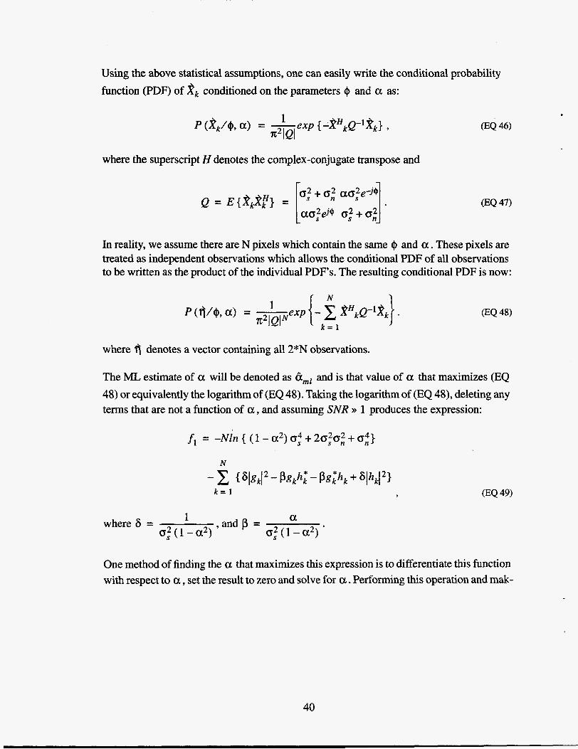
Using the above statistical assumptions, one can easily write the conditional probability function (PDF) of 2 k conditioned on the parameters Q and a as:

where the superscript H denotes the complex-conjugate transpose and

(EQ 47)

In reality, we assume there are N pixels which contain the same Q and a. These pixels are treated as independent observations which allows the conditional PDF of all observations to be written as the product of the individual PDF's. The resulting conditional PDF is now:

where fi denotes a vector containing all 2*N observations.

The ML estimate of a will be denoted as hrnl and is that value of a that maximizes (EQ 48) or equivalently the logarithm of (EQ 48). Taking the logarithm of (EQ 48), deleting any terms that are not a function of a, and assuming SNR P 1 produces the expression:

a where 6 = ,and p = 0 , 2 ( 1 - a 2 ) o,2(1-a2) *

One method of finding the a that maximizes this expression is to differentiate this function with respect to a, set the result to zero and solve €or a. Performing this operation and mak-

40

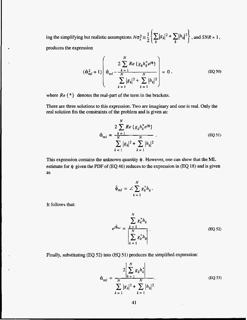
. ing the simplifying but realistic assumptions NG: = { c lgkl I hkl ’} , and S h X >> 1 ,

- 2 k k produces the expression

= 0 ,

where Re { *} denotes the real-part of the term in the brackets.

There are three solutions to this expression. Two are imaginary and one is real. Only the real solution fits the constraints of the problem and is given as:

N

k = l k = 1

This expression contains the unknown quantity 41. However, one can show that the ML estimate for + given the PDF of (EQ 46) reduces to the expression in (EQ 18) and is given as

It follows that:

Finally, substituting (EQ 52) into (EQ 5 1) produces the simplified expression:

(EQ 53)

41

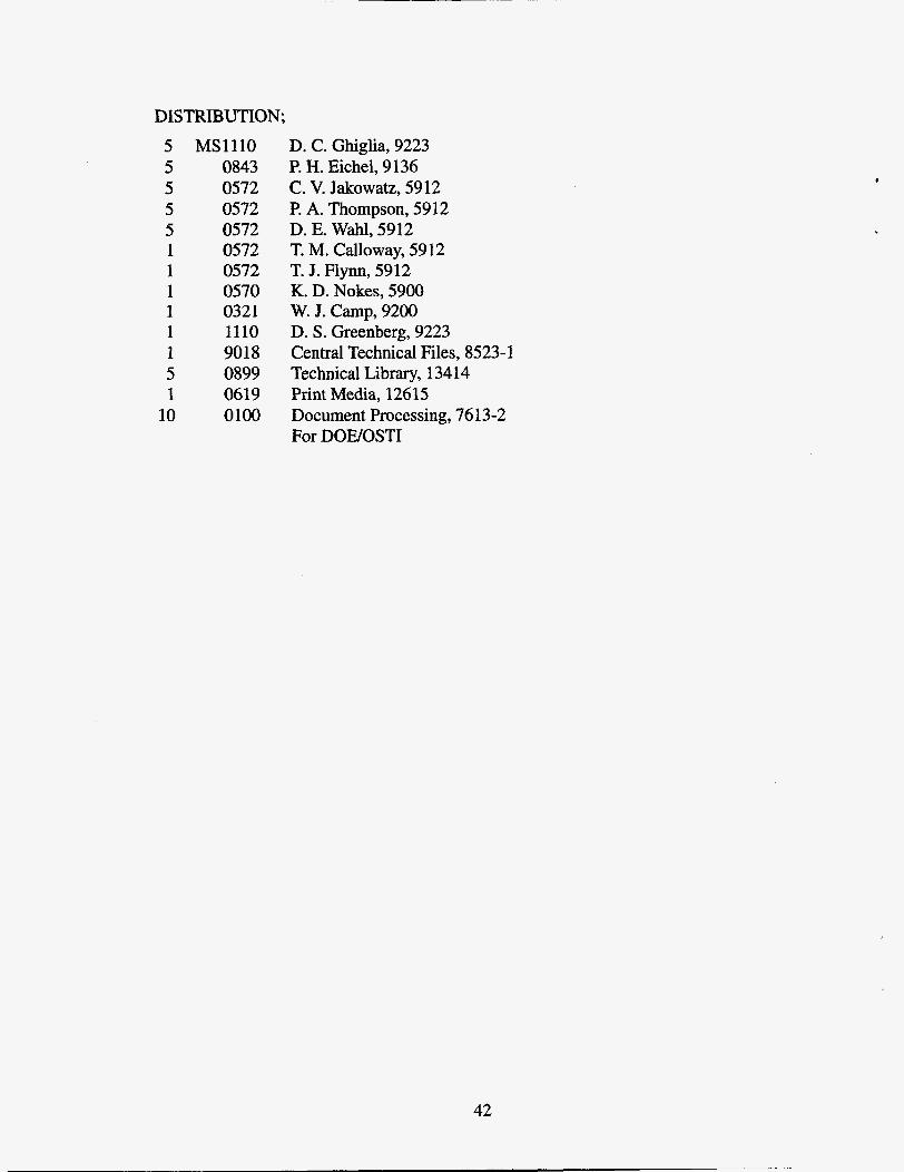
DISTRIBUTION; 5 MSlllO 5 0843 5 0572 5 0572 5 0572 1 0572 1 0572 1 0570 1 0321 1 1110 1 9018 5 0899 1 0619

10 0100

D. C. Ghiglia, 9223 P. H. Eichel, 9136 C. V. Jakowatz, 5912 P. A. Thompson, 5912 D. E. Wahl, 5912 T. M. Calloway, 5912 T. J. Flynn, 5912 K. D. Nokes, 5900 W. J. Camp, 9200 D. S. Greenberg, 9223 Central Technical Files, 8523-1 Technical Library, 13414 Print Media, 12615 Document Processing, 7613-2 For DOEYOSTI

42

spotlight sar interferometry for terrain elevation mapping

Documents