span wagner
TRANSCRIPT

Solution of the Span-Wagner equation of state using
a density-energy state function for fluid-dynamic
simulation of carbon dioxide
Knut Erik Teigen Giljarhus,∗ Svend Tollak Munkejord,∗ and Geir Skaugen∗
SINTEF Energy Research, P.O. Box 4761 Sluppen, NO-7465 Trondheim, Norway
E-mail: [email protected]; [email protected]; [email protected]
Abstract
With the introduction of carbon capture and storage (CCS) as a means to reduce carbon
emissions, a need has arisen for accurate and efficient simulation tools. In this work, we propose
a method for dynamic simulations of carbon dioxide using the Span–Wagner reference equation
of state. The simulations are based on using the density and internal energy as states, which
is a formulation naturally resulting from mass and energy balances. The proposed numerical
method uses information about saturation lines to choose between single-phase and two-phase
equation systems, and is capable of handling phase transitions. To illustrate the potential of the
method, it is applied to simulations of tank depressurization, and to fluid-dynamic simulations
of pipe transport.
∗To whom correspondence should be addressed
1

Introduction
Carbon capture and storage (CCS) has been proposed as a strategy to reduce carbon emissions
to the atmosphere. An important part of the CCS chain is transportation, either in pipelines or in
tanks (on boats, vehicles or trains), from a capture point to a storage site. To ensure efficiency and
safety in these operations, it is important to have accurate simulation tools to control the processes,
and also to perform risk analysis. For instance, an issue with transportation of the supercritical
substance (CO2 is transported at high pressure, in order to minimize pipeline dimensions) is crack
propagation. If a pipeline ruptures, the crack may propagate along the pipe depending on the speed
of the crack relative to the speed of the expansion wave inside the pipe.1,2 To simulate this process,
an accurate model for the flow inside the pipe is needed. Another example is the global trade
of CO2 quotas, which has also been suggested as a means to reduce CO2 emissions.3 From an
economic perspective, it is important to accurately describe the CO2 properties in order to determine
the amount of CO2 stored and transported.
To perform a dynamic simulation, an appropriate mass balance and energy balance is often required
for the system of interest. As an example, consider the depressurization of a rigid tank as illustrated
in Figure 1. We can set up the following mass balance and energy balance for the problem:
Vdρ
dt=−m(T,ρ), (1a)
dUdt
= Q(T )− m(T,ρ)h(T,ρ). (1b)
Here, V is the total volume of the tank, which is constant since the tank is assumed rigid, ρ is
the density, m is the mass flow rate, U is the internal energy, Q is the heat transfer rate, T is
the temperature and h is the specific enthalpy. At each time step of a dynamic simulation, we
know ρ and U . In order to update these, we need to find the temperature and enthalpy from an
equation of state (EOS). The fact that none of the intensive variables are known makes this problem
harder to solve than other formulations. The equilibrium condition represents a maximum in the
2

Q V
m
Figure 1: Schematic illustration of a tank.
entropy of the system.4 This problem has only been sporadically studied in the literature, and
usually for multi-component mixtures. In the context of multi-component mixtures, it is known
as the isoenergetic-isochoric flash, or the UV nnn flash, where nnn is the total number of moles of
each component. In this work, however, we work with systems of the type considered in Eq. (1),
which translates into a ρu problem, where u = U/(ρV ) is the specific internal energy. The first
appearance of the UV nnn-formulation known to the authors is Gani et al.,5 where it is argued that this
formulation has advantages over more traditional approaches. In Flatby et al.,6 dynamic simulations
of propane-butane mixtures in distillation columns were performed with a UV nnn-flash algorithm
based on a Newton-Raphson procedure. In Eckert and Kubícek,7 a rigorous model for simulating
multiple gas-liquid equilibrium stages was developed. This model includes complex multi-phase
systems of type gas-liquid-liquid and gas-liquid-liquid-liquid. New phases are dynamically removed
and added during the simulation. In Müller and Marquardt,8 a faster algorithm for the determination
of the number of phases was introduced. In Saha and Carroll,9 a partial Newton method was used,
along with a novel procedure for generating good initial estimates, to simulate the dynamic filling
of a vessel with nitrogen. In Michelsen,4 a more sophisticated flash algorithm is devised, which
uses stability analysis to determine the number of phases, and a combined solution procedure where
a nested-loop procedure is used together with the Newton method to give a robust method with
good performance. In Gonçalves et al.,10 a similar algorithm was used to simulate storage tanks
and flash drums. In Castier,11 an optimization algorithm is used to directly maximize the entropy.
3

This algorithm is used in Castier 12 to simulate vessels with various fluid mixtures. In Arendsen
and Versteeg,13 the UV nnn formulation is used to simulate a liquefied gas tank with a propane-butane
mixture.
In this work, we are interested in the dynamic simulations involving pure CO2. This allows
several simplifications to be made compared to a multi-component mixture. Most importantly, the
composition is constant (since we only have one component), so saturation curves can be generated
a priori and this information can be utilized during simulation. To obtain the thermodynamic
properties, we use the Span–Wagner equation of state. In Span and Wagner,14 an extensive body
of experimental data for CO2 was reviewed, and an EOS fitted to these data was presented. The
fitting procedure was based on the thermal properties of the single-phase region, the liquid-vapor
saturation curve, the speed of sound, the specific heat capacities, the specific internal energy and
the Joule-Thomson coefficient. The equation gives very accurate results, even in the region around
the critical point, and is now considered as the most accurate reference equation for CO2. It is
for instance used in the NIST Chemistry WebBook.15 There are other alternatives available that
are simpler computationally while retaining most of the accuracy, for instance Huang et al. 16 and
Kim,17 and the proposed method can be used with these equations of state as well.
In this work, we present an efficient method for solving the ρu problem for pure CO2 using the
Span–Wagner (SW) EOS. Although the equation is complicated and contains many terms, we
demonstrate that it is feasible to use it in dynamic simulations. We compare the speed of the method
to an equivalent procedure from the NIST software package REFPROP.18 We also compare the
results to results obtained with simpler equations of state, the stiffened gas (SG) EOS19,20 and
the Peng–Robinson (PR) cubic EOS.21 The presented method can also easily be used with other
equations of state, for instance the two alternative equations of state mentioned above,16,17 or
equations of state for other substances like the reference equation of state for nitrogen from Span
et al..22 It can also be applied to multi-component mixtures, if the composition is constant. To
demonstrate the utility of the proposed method, we apply the algorithm to the dynamic simulation of
4
tank filling, and to a fluid-dynamic simulation of pipe transport. In a fluid-dynamic simulation, there
can be sharp gradients in the solution due to shock waves and other discontinuities. Additionally,
the simulation can potentially be time consuming due to a large number of cells and small time
steps. This puts high demands on the accuracy, robustness and efficiency of the methods used.
Thermodynamics
Thermodynamic properties
If an expression for the (specific) Helmholtz free energy, a(T,ρ) is known, along with its derivatives,
all other thermodynamic properties can be derived from this expression. Important properties in this
work are pressure, specific entropy, specific enthalpy and specific internal energy, which expressed
in terms of the Helmholtz function and its derivatives are
P(T,ρ) = ρ2(
∂a∂ρ
)T, (2)
s(T,ρ) =−(
∂a∂T
)ρ
(3)
h(T,ρ) = a+ρ
(∂a∂ρ
)T−T
(∂a∂T
)ρ
, (4)
u(T,ρ) = a−T(
∂a∂T
)ρ
. (5)
It is common to define a non-dimensional Helmholtz function, φ = a/(RT ), and split this function
into an ideal-gas part, φ0, and a residual part, φr,
φ(τ,δ) = φ0(δ,τ)+φ
r(δ,τ). (6)
This reduced Helmholtz function is expressed in terms of the reduced density, δ = ρ/ρc and the
inverse reduced temperature, τ = Tc/T . ρc and Tc are the critical density and the critical temperature,
5
respectively. The critical properties of CO2 are summarized in Table 1. Expressed in terms of the
reduced Helmholtz energy, the pressure, specific entropy, specific enthalpy and specific internal
energy are
P(τ,δ)ρRT
= 1+δ∂φr
∂δ, (7)
s(τ,δ)R
= τ∂φ
∂τ−φ, (8)
h(τ,δ)RT
= 1+ τ∂φ
∂τ+δ
∂φr
∂δ, (9)
u(τ,δ)RT
= τ∂φ
∂τ. (10)
The Span–Wagner equation of state
The Span–Wagner equation of state is expressed in terms of the reduced Helmholtz energy as
described above. The expression for the ideal part is
φ0(τ,δ) = ln(δ)+a0
1 +a02τ+a0
3 ln(τ)
+8
∑i=4
a0i ln[1− exp(−τθ
0i )].
(11)
The expression for the residual part is
φr(τ,δ) =
7
∑i=1
niδdiτ
ti
+34
∑i=8
niδdiτ
ti exp(−δci)
+39
∑i=35
niδdiτ
ti exp(−αi(δ− εi)2−βi(τ− γi)
2)
+42
∑i=40
ni∆biδexp(−Ci(δ−1)2−Di(τ−1)2),
(12)
6
Temperature (K)
Pre
ssu
re (
MP
a)
225 250 275 300 325 350 375
100
101
102
103
Liquid
Gas
Solid
Supercritical
Figure 2: Phase diagram for CO2.
where ∆ = {(1− τ)+Ai[(δ−1)2]1/(2Bi)}2 +Bi[(δ−1)2]ai . The coefficients a0i , θi
0, ni, ai, bi, βi, Ai,
Bi, Ci and Di can be found in the original paper by Span and Wagner,14 along with expressions for
the derivatives of the Helmholtz function.
We see that the equation contains a total of 51 terms, many of which include logarithms and
exponentials. This means that this is an expensive function to evaluate, and efficient numerical
methods are critical to obtain satisfactory run times for dynamic simulations.
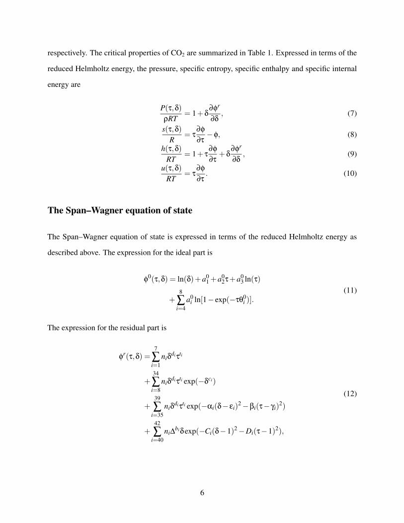
The Span–Wagner equation of state covers the fluid region from the triple-point temperature up
to 1100K and pressures up to 800MPa. In Span and Wagner,14 correlations are also given for the
vapor pressure, melting pressure and sublimation pressure. Figure 2 shows the phase diagram for
CO2 generated using these correlations.
Table 1: Critical properties of CO2.
Property Symbol Value
Critical density ρc 467.6kg/m3
Critical temperature Tc 304.1282KCritical pressure Pc 7.3773MPa
7
Vapor-liquid equilibrium and the ρu algorithm
In an ideally isolated system, all internal processes lead to an increase in the total entropy of the
system. When the entropy reaches its maximum value, the system is at equilibrium. In a system
with liquid and vapor with no chemical reactions, the equilibrium condition is that the temperature,
pressure and the Gibbs free energy must be equal in both phases.
As seen from Eq. (1) for the rigid tank, at each time step of a dynamic simulation, we know the
specific internal energy, uin, and the density, ρin, and want to find the rest of the thermodynamic
properties. If the system is single phase, it is sufficient to solve
u(T,ρin) = uin, (13)
to find the temperature. The rest of the thermodynamic properties can then be found from the
Helmholtz free energy. If the system is vapor-liquid, we need to solve
αρvu(T,ρv)+(1−α)ρlu(T,ρl) = ρinuin, (14a)
αρv +(1−α)ρl = ρin, (14b)
P(T,ρv) = P(T,ρl), (14c)
G(T,ρv) = G(T,ρl), (14d)
to find T , ρv, ρl and α, where α =Vv/V is the vapor volume fraction and G is the Gibbs free energy.
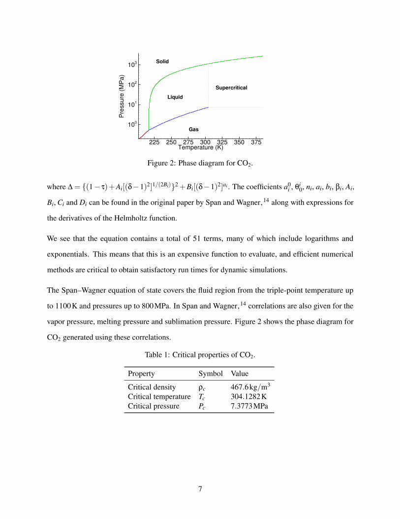
Our algorithm is based on the fact that we can determine whether we have one or two phases based
on the values ρin and uin. Figure 3 shows the phase boundary in the (ρ,u) plane, drawn using the
Span–Wagner equation of state. Before the simulation starts, this phase diagram is generated and
stored as a polygon, where the inside of the polygon denotes the vapor-liquid region. The phase
diagram can be generated by using the Span–Wagner equation of state to find saturation lines using
an iterative procedure, see e.g. Michelsen and Mollerup,23 Chap. 12. During the simulation, it is
8

Internal energy (kJ/kg)
De
nsity (
kg
/m^3
)
400 500 600 700
102
103
Twophase
Liquid
Gas
Critical point
Figure 3: Phase diagram for CO2 in the (ρ,u) plane.
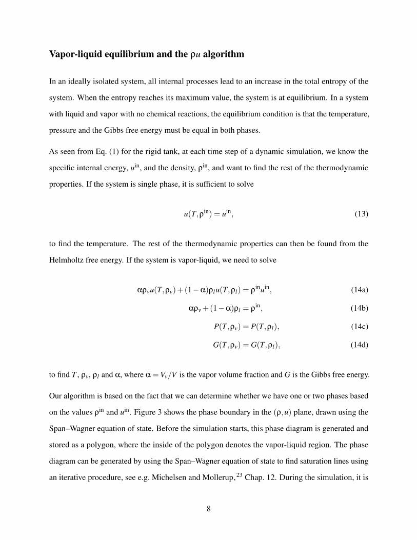
Three crossings, inside
Two crossings, outside
Figure 4: Illustration of the ray-crossing algorithm.
determined if a given point lies within the polygon. If it does, Eq. (14) is solved, and if it is outside,
Eq. (13) is solved. Several different strategies for determining whether a point is inside a polygon
exist, and a good summary is given in Haines.24 Here, we choose a general algorithm based on
ray-crossing. Faster point-in-polygon algorithms exist, for instance by using lookup grids. However,
this introduces higher complexity and higher memory use, and as demonstrated later, the point
inclusion test only constitutes a small part of the total run time. The ray-crossing algorithm works
by shooting a ray from the test point along the x-axis and counting the number of times the ray
crosses the polygon boundary. According to the Jordan curve theorem, every time the boundary
is crossed, the ray switches between inside and outside. If the number of ray crossings is odd, the
point is inside the polygon. See Figure 4 for an illustration. This algorithm has a computational
complexity of O(n), where n is the number of points in the polygon. In this work, we use 200 points.
Since the (ρ,u) polygon is a convex polygon, a simple optimization is to stop the inclusion test after
two crossings have occurred, since by definition a ray shot through a convex polygon can only cross
9

the boundary two times.
After it has been determined if the point lies in the single-phase or vapor-liquid region, the appropri-
ate equation system must be solved. The actual equations are solved using the Newton-Raphson
method. This method can be sensitive to the initial conditions, but since good initial estimates
are often available in dynamic simulations, the fast convergence of this method makes it attractive
for this application. As initial conditions for the solver, we use values from the previous time
step, which are usually close to the actual solution. We evaluate the Jacobian analytically. For the
one-phase system, Eq. (13), the Jacobian is
(∂u∂T
)ρ
= cV , (15)
where cV is the specific heat capacity at constant volume. For the two-phase system, Eq. (14), the
Jacobian is
αρvcV,v +(1−α)ρlcV,l 0 PT,v−PT,l −sv +Pρvρv
+ sl−Pρvρl
αuv +α
ρv
(Pl−T Pρl
)α Pρv
Pρvρg
(1−α)ul +1−α
ρl
(Pl−T Pρl
)1−α −Pρl −Pρl
ρl
ρvuv−ρlul ρv−ρl 0 0
. (16)
The pressure derivatives are derived in terms of the derivatives of the reduced residual Helmholtz
energy as
PT (δ,τ) = ρcδR(1+δφrδ(δ,τ)−δτφ
rδτ(δ,τ)), (17)
Pρ(δ,τ) =RTc
τ(1+2δφ
rδ(δ,τ)+δ
2φ
rδδ(δ,τ)). (18)
If the time step of the dynamical simulation is large, the initial conditions for the Newton iterations
may not be good enough to obtain convergence. This is especially the case for the more complex
vapor-liquid equilibrium equation system. For this system, the required initial conditions are
10

T,ρl,ρg and α. If the Newton-Raphson method fails to converge, it is possible to use estimations for
the saturation conditions to get a better guess for the densities. In Span and Wagner,14 the following
simplified correlations for the saturated liquid density and the saturated vapor density are given,
ln(
ρl
ρc
)=
4
∑i=1
ai
(1− T
Tc
)ti, (19)
ln(
ρg
ρc
)=
5
∑i=1
ai
(1− T
Tc
)ti. (20)
The constants ai and ti are unique for each expression and can be found in the original paper by
Span and Wagner.
Fluid dynamics
Governing equations
As an example of the application of the above algorithm, we consider a 1D flow model of two-phase
CO2. For simplicity, we assume that the two phases have equal velocities. The flow can then be
described by the Euler equations,
∂ρ
∂t+
∂(ρv)∂x
= 0, (21)
∂(ρv)∂t
+∂(P+ρv2)
∂x= 0, (22)
∂(ρe)∂t
+∂[v(ρe+P)]
∂x= 0. (23)
Here, ρ=αgρg+αlρl is the mixture density, v is the velocity and e= u+ 12v2 is the total energy. This
model is often denoted the homogeneous model, and can be accurate if the interphase momentum
transfer is high, for instance in highly dispersed flows. An advantage of using this model is that
the method to solve the ρu problem also can be applied to multi-component mixtures, since the
11

composition is constant. Drift-flux models or two-fluid models can also be used without any
modifications of the thermodynamic solver, but then only for pure CO2.
Since this model is meant to illustrate the ρu problem, we ignore other physical effects like pipe
friction and gravity. These would typically be included as source terms in the above equation
system.
Numerical method
The numerical method we employ is the multi-stage centred approach (MUSTA).25,26 This is a
finite-volume method which retains much of the simplicity of centred schemes, while approaching
the accuracy of more sophisticated upwind schemes. It has also been found to be robust. The
method has been employed for various two-phase flow models, including drift-flux models.27,28 In
the present problem, the complexity lies in the EOS, and the scheme of Titarev and Toro 26 can be
used rather directly.
The system of Eqs. (21) to (23) can be cast in the following form:
∂qqq∂t
+∂ fff (qqq)
∂x= 000, (24)
where qqq = [ρ,ρv,ρe]T is the vector of conserved variables. Employing the finite-volume method,
we obtain the discretized system
qqqm+1j = qqqm
j −∆t∆x
(fff m
j+1/2− fff mj−1/2
), (25)
where qqqmj denotes the numerical approximation to the cell average of the vector of unknowns qqq(x, tm)
in control volume j at time step m. In the MUSTA scheme, the numerical flux at the cell interface is
12

a function of the cell averages on each side:
fff j+1/2 = fff MUSTA(qqq j,qqq j+1). (26)
Further details can be found in Titarev and Toro 26 and Munkejord et al. 27
The numerical method, Eq. (25), is subject to the Courant–Friedrichs–Lewy (CFL) stability condi-
tion. The CFL number is
R =‖λ‖∞∆t
∆x, (27)
where ‖λ‖∞ is the maximum eigenvalue of the flux Jacobian matrix of the model (24) in the
computational domain. Here we have
‖λ‖∞ = max|v±C|, (28)
where C is the speed of sound. Note that in the two-phase region, the sound speed of the mixture is
the combined result of the thermodynamic relations and the flow model. Further, in large parts of
the two-phase region, the sound speed of the mixture is smaller than that of pure gas or pure liquid.
For the present homogeneous flow model, the mixture speed of sound can be calculated analytically
using Eq. (6.15) of Flåtten and Lund,29
C−2mix = ρmix(Zp +ZpT +ZpT µ), (29)
Zp =αg
ρgcg+
αl
ρlcl, (30)
ZpT =cp,gcp,lTcp,g + cp,l
(Γl
ρlcl−
Γg
ρgcg
)2
, (31)
ZpT µ =ρmixT
cp,g + cp,l
(ρg−ρl
ρgρl(hg−hl)(cp,g + cp,l)+
Γgcp,g
ρgC2g+
Γlcp,l
ρlC2l
)2
, (32)
13

Entropy (kJ/kgK)
Pre
ssu
re (
MP
a)
3 3.5 4
2
4
6
810
Twophase
Gas Liquid
Figure 5: Phase diagram for CO2 in the (P,s) plane.
where Γi is the Grüneisen coefficient,
Γi =1ρi
(∂p∂ui
)ρi
. (33)
Boundary conditions
In a fluid-dynamic simulation, boundary conditions must be specified at the domain boundaries.
Here, we implement the boundaries using ghost cells. The specified-pressure boundary condition
requires extra care. For this boundary condition, we assume an isentropic process, which means
that the specific entropy, s, in the ghost cell is taken to be the same value as the first inner cell.
The pressure is set to the specified value. The rest of the variables must then be calculated in
the ghost cell. The equilibrium value for this Ps problem corresponds to a global minimum in
the enthalpy of the system.4 However, here we employ the same approach as for the ρu problem.
Before the simulation starts, the saturation curve is drawn in the (P,s) plane. This curve is shown in
Figure 5. This curve is then used to determine which equation system has to be solved using the
14

point-in-polygon algorithm. For a single-phase system, the equation system to solve is
P(T,ρ) = Pin, (34a)
s(T,ρ) = sin, (34b)
with T and ρ as unknowns. For a two-phase system, we know that the pressure is the vapor pressure,
and we can then determine the temperature and densities directly from the saturation line. It then
remains to find the vapor mass fraction, x, which is found by solving
xsg(T,ρg)+(1− x)sl(T,ρl) = sin. (35)
To solve the equations, we use the Newton-Raphson method with numerical derivatives.
Results
This section presents some results from using the proposed algorithm. First, a convergence test is pre-
sented to test correctness and efficiency. Then, the algorithm is applied to the tank depressurization
problem from the introduction. Finally, some fluid dynamics simulations are presented.
Convergence test
To get an indication of the robustness and performance of the proposed approach, a set of prob-
lems was generated by choosing pressures and temperatures, calculating the density and internal
energy, and then checking the necessary number of iterations for the algorithm to converge to the
initial pressure and temperature. A comparison is also being made to the NIST software package
REFPROP,18 which contains a subroutine DEFLSH that also solves the ρu problem.
Two sets of pressures and temperatures are considered. First, we choose 10000 points in the
15

single-phase regime, with temperatures ranging from 220K to 350K and pressures ranging from
0.1MPa to 20MPa. Second, we choose 10000 points along the saturation line with a gas fraction
of 0.5 to test convergence in the two-phase regime. In dynamic simulations, the results from the
previous time step can often provide a good initial estimate for the non-linear solver. Here, we get
the initial condition by perturbing the exact solution by 10%.
The algorithm was able to find the correct solution for all problems, even in the vicinity of the critical
region. The total runtime and average number of iterations are given in Table 2. The programs
are written in the Fortran programming language, and compiled with the GNU Fortran compiler
with the -O3 optimization flag. The times were taken using the cpu_time subroutine on an Intel(R)
Core(TM)2 Duo T7700 CPU. The two-phase problems took about 24 times longer to complete.
This is because they require more iterations to converge coupled with a more expensive function
evaluation. Overall, the total runtime is low considering the number of problems, and is considered
adequate for dynamic simulations. The runtime is dominated by the solution of the non-linear
system. For the single-phase cases, the point-inclusion test represents about 3% of the total runtime,
while for the two-phase cases, only about 0.2% of the time is spent in the point-inclusion test. This
justifies the use of the general point-in-polygon algorithm over more sophisticated approaches.
The REFPROP program takes significantly more time to find the solution. For the single-phase case,
REFPROP is about 20 times slower, while for the two-phase case, REFPROP is about 16 times
slower. Additionally, REFPROP failed to converge for single-phase problems near the melting line.
Table 2: Comparison of total runtime and average number of iterations for solving 10000 ρu-problems in the single-phase and two-phase regimes.
Regime Total time (s) Average # of iterations REFPROP (s)
Single-phase 0.39 2.5 7.54Two-phase 9.25 5.0 148.35
16

Tank simulations
In this section, we use the tank model from the introduction, Eq. (1), to simulate the depressurization
of a tank. To close the tank model, we need expressions for the heat transfer rate, Q, and the mass
flow rate, m. We model the heat transfer as the heat transfer rate multiplied with the temperature
difference between the tank temperature and the ambient temperature, Tamb,
Q(T ) = ηA(Tamb−T ) , (36)
where η is the overall heat-transfer coefficient and A is the surface area of the tank. The flow rate is
modeled using a valve equation,
m = Kv√
ρ(P−Pamb), (37)
where Kv is a flow coefficient for the valve and Pamb is the ambient pressure. To solve the equations,
we use the DASSL differential algebraic equation solver.30
As a test case, we consider a cylindrical tank with diameter 0.2m and height 1.0m, with initial state
P0 = 80bar and T0 = 25◦C. The ambient conditions are Pamb = 6bar and Tamb = 5◦C. A moderate
value of ηA = 10W/K is used, and the valve coefficient is set to Kv = 8×10⁻⁷ m2. At t = 0, the
valve is opened to the surroundings. Note that initially, CO2 is in a compressible liquid state, above
the critical pressure, while at steady state it will reach the ambient condition which is in the vapor
region. This is a challenging test case, since it covers pure liquid, transition to two-phase and finally
transition to pure vapor.
Figure 6 shows the transient development of the contained mass inside the tank, the pressure, the
temperature and the vapor volume fraction. There is a fast reduction in temperature and pressure
down to the saturation line. The CO2 then starts to evaporate, and the temperature and pressure
continues to decrease until all the liquid has evaporated. When all the liquid has evaporated, the
pressure in the vessel has reached about 7.7bar. Now, heat transfer starts to dominate, and the gas
is heated by the ambient and further expanded until the final state of 5◦C and 6bar is reached. In
17

Time (h)
P (
ba
r), T
(°C
), M
(kg
)
α
0 0.1 0.2 0.3 0.4 0.5 0.6
40
20
0
20
40
60
80
0
0.2
0.4
0.6
0.8
1
P
T
M
α
Figure 6: Depressurization of a CO2 tank. Pressure (P), temperature (T ), mass (M) and vaporvolume fraction (α) as a function of time.
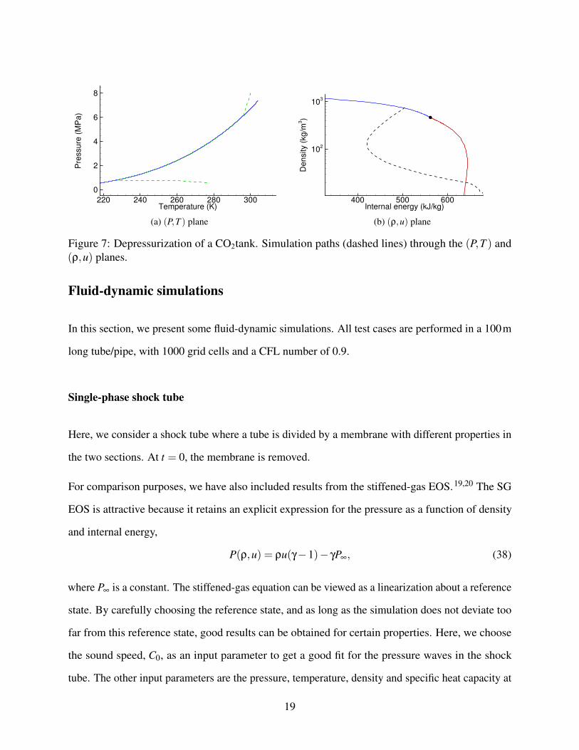
Figure 7a the same development is shown in a pressure-temperature diagram. The vapor pressure
line is indicated as a solid line and the simulation path is shown as a dashed line. The initial point
of the simulation is in the liquid region. Saturated conditions are reached after only about 10s at
approximately 61bar and 296K where vapor starts forming due to expansion. At 7.7bar all the
(remaining) liquid has evaporated and the vapor is superheated until the ambient temperature is
reached. The same process is also shown in the (ρ,u)-plane in Figure 7b. The initial state is just
above the saturation line for liquid internal specific energy. Then it expands into, and through, the
two-phase region and finally into the vapor region where it is further expanded to reach ambient
temperature and pressure. In the first part of the expansion, the internal energy decreases due to the
fast initial expansion due to the opening of the valve. After this initial abrupt decrease in pressure,
the heat transfer starts to dominate, and the internal energy starts to increase. The density continues
to decrease due to the open valve. When all the liquid has evaporated, the vapor is superheated and
expanded until the ambient temperature and pressure is reached. The expansion is faster in the pure
vapor phase due to the higher compressibility of the vapor.
18
Temperature (K)
Pre
ssu
re (
MP
a)
220 240 260 280 300
0
2
4
6
8
(a) (P,T ) plane
Internal energy (kJ/kg)
De
nsity (
kg
/m3)
400 500 600
102
103
(b) (ρ,u) plane
Figure 7: Depressurization of a CO2tank. Simulation paths (dashed lines) through the (P,T ) and(ρ,u) planes.
Fluid-dynamic simulations
In this section, we present some fluid-dynamic simulations. All test cases are performed in a 100m
long tube/pipe, with 1000 grid cells and a CFL number of 0.9.
Single-phase shock tube
Here, we consider a shock tube where a tube is divided by a membrane with different properties in
the two sections. At t = 0, the membrane is removed.
For comparison purposes, we have also included results from the stiffened-gas EOS.19,20 The SG
EOS is attractive because it retains an explicit expression for the pressure as a function of density
and internal energy,
P(ρ,u) = ρu(γ−1)− γP∞, (38)
where P∞ is a constant. The stiffened-gas equation can be viewed as a linearization about a reference
state. By carefully choosing the reference state, and as long as the simulation does not deviate too
far from this reference state, good results can be obtained for certain properties. Here, we choose
the sound speed, C0, as an input parameter to get a good fit for the pressure waves in the shock
tube. The other input parameters are the pressure, temperature, density and specific heat capacity at
19
constant pressure. The rest of the parameters in Eq. (38) are then found from
γ =C2
0cP,0T0
+1, (39)
cV =cP,0
γ, (40)
P∞ = ρ0cV T0(γ−1)−P0. (41)
As a reference state, we use the arithmetic mean of the two tube sections.
Here, we look at a case in the gas phase. The left section is at P = 3MPa and the right section is
at P = 1MPa, with a uniform temperature of T = 300K. The results at t = 0.08s are plotted in
Figure 8. Due to the pressure difference, the gas starts flowing towards the right. A shock wave also
propagates to the right, while a rarefaction wave propagates to the left. We also observe a contact
discontinuity in the density and temperature. Our ρu solver is clearly capable of finding the solution
even in the presence of sharp gradients. Typically, 2–4 iterations are required in the non-linear
solver. We also observe good agreement with the stiffened-gas equation for the pressure waves. For
the temperature and density, however, the agreement is not as good, which is due to the inability of
the stiffened-gas equation to fully capture the thermodynamic behavior of CO2.
The numerical method should converge as the grid size is increased, and no oscillations should be
introduced. A demonstration of convergence with grid refinement is shown in Figure 9.
Transition from one-phase to two-phase
Transport of CO2 in a gaseous state is inefficient because of the low density which gives a relatively
high pressure drop per unit length of the pipe. Hence, the transport of CO2 is typically done in a
dense liquid-like state, since this is the most energy efficient condition.31 The pressure should also
be higher than the critical pressure, to avoid the possibility of evaporation if temperature changes
occur along the pipeline. However, during events such as startup and shutdown, or due to critical
events such as pipe rupture, the pressure can quickly drop causing transition to two-phase. Here, we
20

0 20 40 60 80 100Pipe length (m)
1.0
1.5
2.0
2.5
3.0
Pres
sure
(MPa
) Span-WagnerStiffened gas
0 20 40 60 80 100Pipe length (m)
260
280
300
320
340
Tem
pera
ture
(K)
0 20 40 60 80 100Pipe length (m)
20
30
40
50
60
Den
sity
(kg/
m3
)
0 20 40 60 80 100Pipe length (m)
0
20
40
60
80
100
120
Velo
city
(m/s
)
Figure 8: Shock tube test case in the gas phase. Comparison between Span–Wagner and stiffenedgas at t = 0.08s.
70 72 74 76 78 80 82Pipe length (m)
0.91.01.11.21.31.41.51.61.7
Pres
sure
(MPa
) 501002003200
Figure 9: Shock tube test case in the gas phase. Convergence of the pressure with grid refinement.
21

consider such a depressurization case in which the pipe is initially at 10MPa and T = 300K. At
t = 0, the pressure at the right-hand boundary is set to 3MPa. A pressure wave will propagate into
the pipe and induce a flow towards the right-hand boundary. Due to the reduction in pressure, some
of the liquid will evaporate.
The results at t = 0.2s is shown in Figure 10. At the right boundary, the liquid evaporates and the
gas fraction eventually reaches a value of 0.48. We also see that the pressure wave splits in two
parts. The first part is from the initial pressure down to the vapor pressure, and the second part is
in the two-phase region from the vapor pressure down to the outlet pressure. A similar case was
considered in Lund et al. 32 with the SG EOS. As discussed in that article, the split in the pressure
wave is due to a discontinuity in the sound speed when going from pure liquid to two-phase. This is
caused by the assumption of equilibrium in pressure, temperature and chemical potential, and is
further discussed in Flåtten and Lund.29
Figure 10 shows results for both the SW EOS and the PR EOS. We see that there is an appreciable
difference in the results. In particular, the liquid fraction at the end of the domain is very different.
Accurate prediction of the liquid fraction can be important, for instance to determine the amount of
carbon dioxide released due to a pipeline fracture.
The methods used for solving the ρu problem for the PR EOS are the flash algorithms described
in e.g. Michelsen.4 The total time of the PR simulation was 20m54s. For the simulation with
the SW EOS, the total time was 29m13s. Since the flash algorithms used for the PR EOS are
computationally expensive, the PR simulation has similar runtimes as the method presented here,
even though the SW EOS is a significantly more complex EOS. We note that the method presented
in this work could also be applied to the PR EOS, although that was not attempted here. We also
note that the runtimes are obviously dependent on the implementation, so the numbers are only
intended as an indication of the computational complexity.
22

0 20 40 60 80 100Pipe length (m)
3456789
10Pr
essu
re (M
Pa) Span-Wagner
Peng-Robinson
0 20 40 60 80 100Pipe length (m)
265270275280285290295300
Tem
pera
ture
(K)
75 80 85 90 95 100Pipe length (m)
0.2
0.4
0.6
0.8
1.0Li
quid
frac
tion
Figure 10: Two-phase depressurization test case. t = 0.2s. Note that the liquid fraction is onlyplotted for the right end of the domain.
Conclusions
In this work, an algorithm for performing dynamic simulations of systems with pure CO2 with
the Span–Wagner equation of state was presented. The algorithm assumes a density-energy state
function and explicitly employs information about the saturation lines which allows for a simpler
and more efficient implementation than other approaches. The algorithm was applied to two
different problems, a tank model and a fluid-dynamic pipe flow model. The method was shown to
be both robust and efficient, and it was demonstrated that the method tackles both single-phase and
vapor-liquid problems, and transition between phases.
Further work with respect to the ρu algorithm could be to apply it to other equations of state, either
to reference equations for other substances or to simpler equations like the cubic equations of state.
It could also be tested for multi-component problems where the composition is constant. A similar
approach was for instance used in Arendsen and Versteeg 13 and Flatby et al. 6 for tank simulations.
For the homogeneous model used in this work for the fluid dynamics, the composition is constant
23
since the gas and liquid velocities are equal. Hence, the presented method can be used to compute
multi-component mixtures together with this fluid dynamic model. To determine which situations
this model can be applied to requires experimental validation.
As demonstrated by the final test case, the sound velocity is discontinuous when going from single-
phase to two-phase flow for a full equilibrium model. In Flåtten and Lund,29 it is shown that
relaxation models can be used to remedy this issue. It would be interesting to see if this concept can
be used together with the Span–Wagner equation of state.
Finally, only the presence of gas and liquid was considered in this work. It is well known that
dry ice can form for severe depressurizations. The model developed here can be extended with
additional equation systems for the solid-vapor and the solid-liquid phases. Together with a model
for the thermodynamic properties of the solid phase, this could provide a solid-liquid-vapor model
which could be solved with an extension of the presented method.
Acknowledgement
This publication has been produced with support from the BIGCCS Centre, performed under the
Norwegian research program Centres for Environment-Friendly Energy Research (FME). The
authors acknowledge the following partners for their contributions: Aker Solutions, ConocoPhillips,
Det Norske Veritas, Gassco, Hydro, Shell, Statkraft, Statoil, TOTAL, GDF SUEZ and the Research
Council of Norway (193816/S60).
We are grateful to our colleagues Øivind Wilhelmsen, Tore Flåtten, Halvor Lund for fruitful
discussions, and Morten Hammer for his assistance with some of the simulations.
We thank the anonymous reviewers for carefully reading the manuscript and making several useful
remarks.
24
References
1. Aihara, S.; Misawa, K. Numerical simulation of unstable crack propagation and arrest in CO2
pipelines. The First International Forum on the Transportation of CO2 in Pipelines. Newcastle,
UK, 2010.
2. Berstad, T.; Dørum, C.; Jakobsen, J. P.; Kragset, S.; Li, H.; Lund, H.; Morin, A.; Munke-
jord, S. T.; Mølnvik, M. J.; Nordhagen, H. O.; Østby, E. CO2 pipeline integrity: A new
evaluation methodology. Energy Procedia 2011, To appear.
3. Chichilnisky, G.; Heal, G. Markets for Tradeable CO2 Emission Quotas Principles and Practice;
OECD Economics Department Working Papers 153, 1995.
4. Michelsen, M. L. State function based flash specifications. Fluid Phase Equilib. 1999, 158-160,
617 – 626.
5. Gani, R.; Perregaard, J.; Johansen, H. Simulation strategies for design and analysis of complex
chemical processes. Chem. Eng. Res. and Design 1990, 68, 407–417.
6. Flatby, P.; Lundström, P.; Skogestad, S. Rigorous dynamic simulation of distillation columns
based on UV-flash. IFAC Symposium ADCHEM’94, Kyoto, Japan. 1994.
7. Eckert, E.; Kubícek, M. Modelling of dynamics for multiple liquid–vapour equilibrium stage.
Chem. Eng. Sci. 1994, 49, 1783 – 1788.
8. Müller, D.; Marquardt, W. Dynamic multiple-phase flash simulation: Global stability analysis
versus quick phase determination. Comput. Chem. Eng. 1997, 21, S817 – S822.
9. Saha, S.; Carroll, J. J. The isoenergetic-isochoric flash. Fluid Phase Equilib. 1997, 138, 23 –
41.
10. Gonçalves, F.; Castier, M.; Araújo, O. Dynamic simulation of flash drums using rigorous
physical property calculations. Braz. J. Chem. Eng. 2007, 24, 277–286.
25

11. Castier, M. Solution of the isochoric-isoenergetic flash problem by direct entropy maximization.
Fluid Phase Equilib. 2009, 276, 7 – 17.
12. Castier, M. Dynamic simulation of fluids in vessels via entropy maximization. J. Ind. Eng.
Chem. 2010, 16, 122 – 129.
13. Arendsen, A. R. J.; Versteeg, G. F. Dynamic Thermodynamics with Internal Energy, Volume,
and Amount of Moles as States: Application to Liquefied Gas Tank. Ind. Eng. Chem. Res. 2009,
48, 3167–3176.
14. Span, R.; Wagner, W. A New Equation of State for Carbon Dioxide Covering the Fluid Region
from the Triple-Point Temperature to 1100 K at Pressures up to 800 MPa. J. Phys. Chem. Ref.
Data 1996, 25, 1509–1596.
15. Linstrom, P., Mallard, W., Eds. NIST Chemistry WebBook; National Institute of Standards and
Technology, Gaithersburg MD, 20899, 2011; http://webbook.nist.gov, (retrieved February 16,
2011).
16. Huang, F.; Li, M.; Lee, L. L.; Starling, K. E.; Chung, F. T. H. An accurate equation of state for
carbon dioxide. J. Chem. Eng. Japan 1975, 18, 490–496.
17. Kim, Y. Equation of state for carbon dioxide. J. Mech. Sci. Tech. 2007, 21, 799–803.
18. Lemmon, E. W.; Huber, M. L.; McLinden, M. O. NIST Standard Reference Database 23:
Reference Fluid Thermodynamic and Transport Properties-REFPROP, Version 9.0, National
Institute of Standards and Technology, Standard Reference Data Program. 2010, Gaithersburg.
19. Menikoff, R.; Plohr, B. J. The Riemann problem for fluid flow of real materials. Rev. Mod. Phys.
1989, 61, 75–130.
20. Menikoff, R. Shock Wave Science and Technology Reference Library, Volume 2 – Solids;
Springer-Verlag: Berlin, 2007; pp 143–188.
26
21. Peng, D.; Robinson, D. B. A New Two-Constant Equation of State. Ind. Eng. Chem. Funda-
mentals 1976, 15, 59–64.
22. Span, R.; Lemmon, E. W.; Jacobsen, R. T.; Wagner, W.; Yokozeki, A. A Reference Equation of
State for the Thermodynamic Properties of Nitrogen for Temperatures from 63.151 to 1000 K
and Pressures to 2200 MPa. J. Phys. Chem. Ref. Data 2000, 29, 1361–1433.
23. Michelsen, M. L.; Mollerup, J. Thermodynamic Models: Fundamentals and Computational
Aspects; Tie-Line Publications, 2007.
24. Haines, E. Graphics Gems IV: “Point in polygon strategies”; Academic Press, 1994.
25. Toro, E. F. MUSTA: A multi-stage numerical flux. Appl. Numer. Math. 2006, 56, 1464–1479.
26. Titarev, V. A.; Toro, E. F. MUSTA schemes for multi-dimensional hyperbolic systems: analysis
and improvements. Int. J. Numer. Meth. Fluids 2005, 49, 117–147.
27. Munkejord, S. T.; Evje, S.; Flåtten, T. The multi-stage centred-scheme approach applied to a
drift-flux two-phase flow model. Int. J. Numer. Meth. Fluids 2006, 52, 679–705.
28. Munkejord, S. T.; Jakobsen, J. P.; Austegard, A.; Mølnvik, M. J. Thermo- and fluid-dynamical
modelling of two-phase multi-component carbon dioxide mixtures. Int. J. Greenh. Gas Cont.
2010, 4, 589–596.
29. Flåtten, T.; Lund, H. Relaxation two-phase flow models and the subcharacteristic condition.
Math. Models Methods Appl. Sci. 2011, Accepted.
30. Petzold, L. Description of DASSL: a differential/algebraic system solver. 1982, SAND-82-8637,
Sandia National Laboratories.
31. Zhang, Z.; Wang, G.; Massarotto, P.; Rudolph, V. Optimization of pipeline transport for CO2
sequestration. Energy Convers. Manage. 2006, 47, 702 – 715.
27
32. Lund, H.; Flåtten, T.; Munkejord, S. T. Depressurization of carbon dioxide in pipelines - models
and methods. Energy Procedia 2011, To appear.
28