21st Computer Vision Winter WorkshopLuka Cehovin, Rok Mandeljc, Vitomir Struc (eds.)Rimske Toplice, Slovenia, February 3–5, 2016

Solving Dense Image Matching in Real-Time using Discrete-ContinuousOptimization

Alexander Shekhovtsov, Christian Reinbacher, Gottfried Graber and Thomas PockInstitute for Computer Graphics and Vision, Graz University of Technology

{shekhovtsov,reinbacher,graber,pock}@icg.tugraz.at

Abstract. Dense image matching is a fundamental low-level problem in Computer Vision, which has receivedtremendous attention from both discrete and continuousoptimization communities. The goal of this paper is tocombine the advantages of discrete and continuous op-timization in a coherent framework. We devise a modelbased on energy minimization, to be optimized by bothdiscrete and continuous algorithms in a consistent way.In the discrete setting, we propose a novel optimizationalgorithm that can be massively parallelized. In the con-tinuous setting we tackle the problem of non-convex reg-ularizers by a formulation based on differences of convexfunctions. The resulting hybrid discrete-continuous algo-rithm can be efficiently accelerated by modern GPUs andwe demonstrate its real-time performance for the applica-tions of dense stereo matching and optical flow.

1. IntroductionThe dense image matching problem is one of the most

basic problems in computer vision: The goal is to findmatching pixels in two (or more) images. The applica-tions include stereo, optical flow, medical image registra-tion, face recognition [1], etc. Since the matching problemis inherently ill-posed, typically optimization is involvedin solving it. We can distinguish two fundamentally dif-ferent approaches: discrete and continuous optimization.Whereas discrete approaches (see [14] for a recent com-parison) assign a distinct label to each output pixel, con-tinuous approaches try to solve for a function using thecalculus of variations [6, 8, 21]. Both approaches havereceived enormous attention, and there exist state-of-the-art algorithms in both camps: continuous [23, 24, 28] anddiscrete [18, 30]. Due to the specific mathematical toolsavailable to solve the problems (discrete combinatorial op-timization vs. continuous calculus of variations), both ap-proaches have distinct advantages and disadvantages.

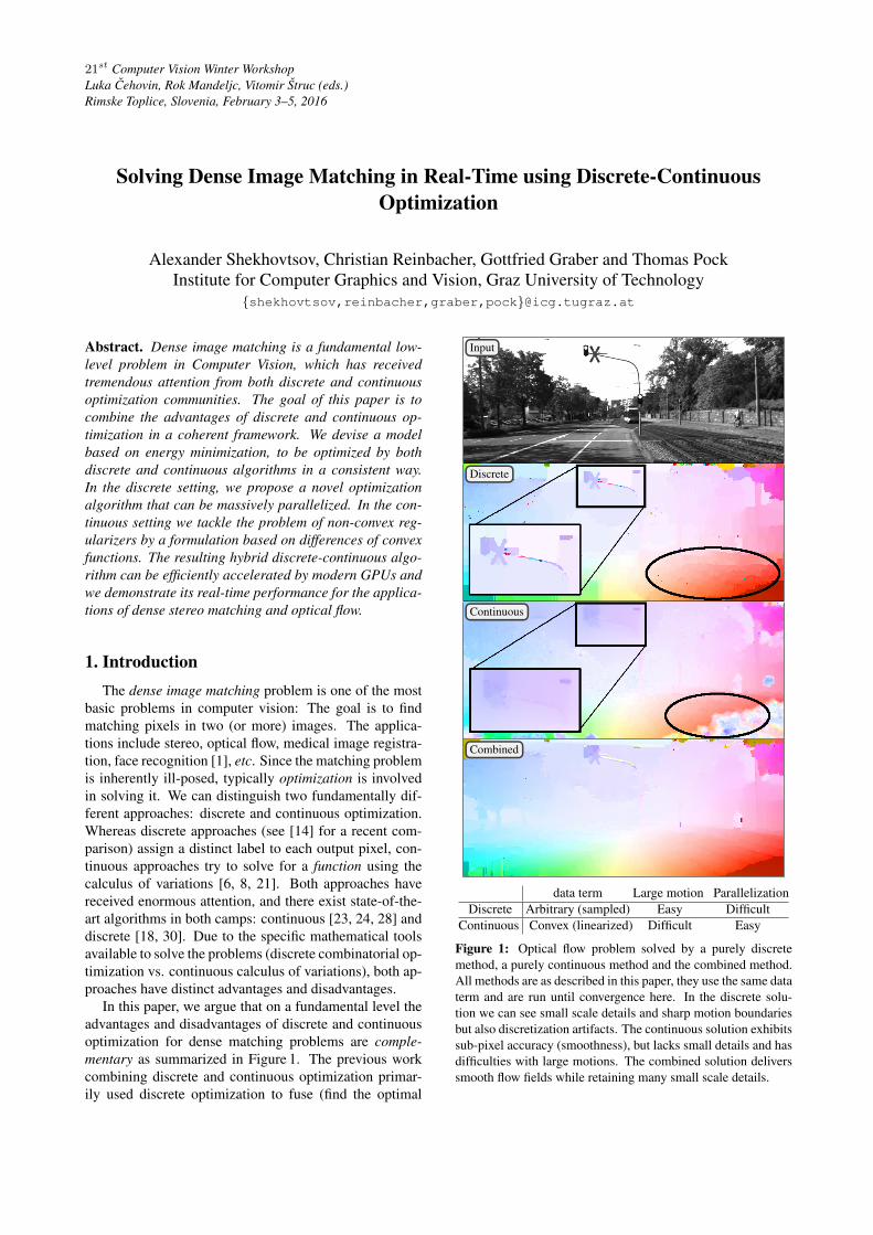
In this paper, we argue that on a fundamental level theadvantages and disadvantages of discrete and continuousoptimization for dense matching problems are comple-mentary as summarized in Figure 1. The previous workcombining discrete and continuous optimization primar-ily used discrete optimization to fuse (find the optimal

Input

Discrete

Continuous

Combined

data term Large motion ParallelizationDiscrete Arbitrary (sampled) Easy Difficult

Continuous Convex (linearized) Difficult Easy

Figure 1: Optical flow problem solved by a purely discretemethod, a purely continuous method and the combined method.All methods are as described in this paper, they use the same dataterm and are run until convergence here. In the discrete solu-tion we can see small scale details and sharp motion boundariesbut also discretization artifacts. The continuous solution exhibitssub-pixel accuracy (smoothness), but lacks small details and hasdifficulties with large motions. The combined solution deliverssmooth flow fields while retaining many small scale details.

crossover) of candidate continuous proposals, e.g. [36, 30](stereo) and [25] (flow). The latter additionally per-forms local continuous optimization of the so-found solu-tion. Many works also alternate between continuous anddiscrete optimizations, addressing a Mumford-Shah-likemodel, e.g., [5]. Similarly to [25] we introduce a continu-ous energy which is optimized using a combined method.However, we work with a full (non-local) discretization ofthis model and propose new parallel optimization meth-ods.

The basic difference in discrete and continuous ap-proaches lies in the handling of the data term. The dataterm is a measure how well the solution (i.e. value of apixel) fits the underlying measurement (i.e. input images).In the discrete setting, the solution takes discrete labels,and hence the number of labels is finite. Typically thedata cost is precomputed for all possible labels. The dis-crete optimization then uses the data cost to find the opti-mal label for each pixel according to a suitable model inan energy minimization framework. We point out that dueto the sampling in both label space and spatial domain, thediscrete algorithm has access to the full information at ev-ery step. I.e. it deals with a global optimization model andin some lucky cases can find a globally optimal solution toit or provide an approximation ratio or partial optimalityguarantees [27].

In the continuous setting, the solution is a continuousfunction. This means it is not possible to precompute thedata cost; an infinite number of solutions would requireinfinite amount of memory. More importantly, the datacost is a non-convex function stemming from the similar-ity measure between the images. In order to make theoptimization problem tractable, a popular approach is thelinearization of the data cost. However, this introducesa range of new problems, namely the inability to dealwith large motions due to the fact that the linearization isvalid only in a small neighborhood around the lineariza-tion point. Most continuous methods relying on lineariza-tion therefore use a coarse-to-fine framework in an attemptto overcome this problem [4]. One exception is a recentwork [16], which can handle piece-wise linear data termsand truncated TV regularization.

Our goal in this paper is to combine the advantages ofboth approaches, as well as real-time performance, whichimposes tough constraints on both methods resulting in anumber of challenges:

Challenges The discrete optimization method needs tobe highly parallel and able to couple the noisy / ambigu-ous data over large areas. The continuous energy shouldbe a refinement of the discrete energy so that we can evalu-ate the two-phase optimization in terms of a single energyfunction. The continuous method needs to handle robust(truncated) regularization terms.

Contribution Towards the posed challenges, we pro-pose: i) a new method for the discrete problem, working inthe dual (i.e. making equivalent changes of the data costvolume), in parallel on multiple chains; ii) a continuous

optimization method, reducing non-convex regularizers toa primal-dual method with non-linear operators [31]; iii)an efficient implementation of both methods on GPU andproof of concept experiments showing advantages of thecombined approach.

2. MethodIn this section we will describe our two-step approach

to the dense image matching problem. To combine thepreviously discussed advantages of discrete and continu-ous optimization methods it is essential to minimize thesame energy in both optimization methods. Starting froma continuous energy formulation in § 2.1, we first showhow to discretize the energy in § 2.2 and subsequentlyminimize it using a novel discrete parallel block coordi-nate descent, described in § 2.3. The output of this algo-rithm will be the input to a refinement method which isposed as a continuous optimization problem, solved by anon-linear primal-dual algorithm described in § 2.4.

2.1. Model

Let us formally define the dense image matching prob-lem to be addressed by the discrete-continuous optimiza-tion approach. In both formulations we consider that theimage domain is a discrete set of pixels V . The continuousformulation has continuous ranged variables u = (uki ∈R | k = 1, . . . d, i ∈ V), where d = 1, 2 for stereo / flow,respectively. The matching problem is formulated as

minu∈U

[E(u) = D(u) +R(Au)

], (1)

where U = Rd×V ; D is the data term and R(Au) is aregularizer (A is a linear operator explained below). Thediscrete formulation will quantize variable ranges.

Data Term We assume D(u) =∑i∈V Di(ui), where

Di : Rd → R encodes the deviation of ui from some un-derlying measurement. A usual choice for dense imagematching are robust filters like Census Transform or Nor-malized Cross Correlation, computed on a small windowaround a pixel. This data term is non-convex in u andpiecewise linear. In the discrete setting, the data term issampled at discrete locations, in the continuous setting,the data term is convexified by linearizing or approximat-ing it around the current solution. The details will be de-scribed in the respective sections.

Regularization Term The regularizer encodes prop-erties of the solution of the energy minimization like localsmoothness or preservation of sharp edges. The choice ofthis term is crucial in practice, since the data term may beunreliable or uninformative in large areas of dense match-ing problems. We assume

R(Au) =∑ij∈E

ωij

d∑k=1

r((Auk)ij), (2)

where E ⊂ V × V is the set of edges, i.e., pairs ofneighboring pixels; linear operator A : RV → RE : uk 7→

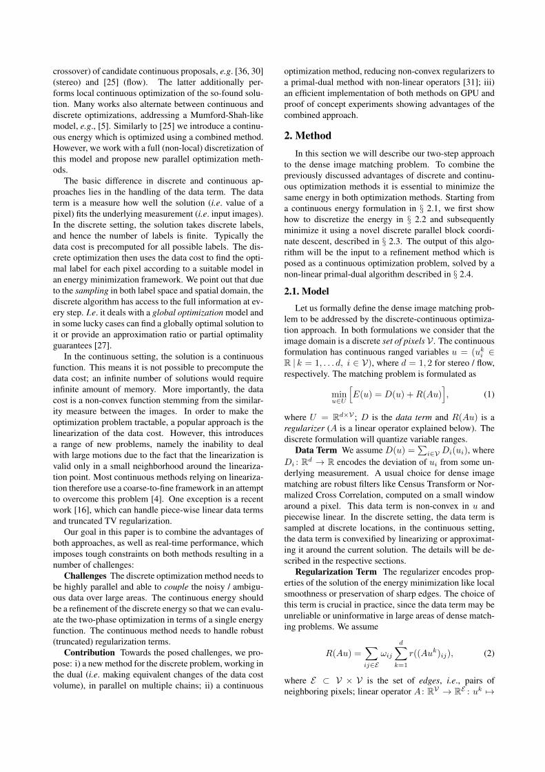
(uki − ukj ∈ R | ∀ij ∈ E) essentially computes gradientsalong the edges in E for the solution dimension k; the gra-dients are penalized by the penalty function r : R → Rand ωij are image dependent per-edge strength weights,reducing the penalty around sharp edges. Our particularchoice for the penalty function r is depicted in Fig. 2. Wechose to use a truncated norm which has shown to be ro-bust against noise that one typically encounters in densematching problems. It generalizes truncated Total Vari-ation in the continuous setting. In the discrete setting itgeneralizes the P1-P2 penalty model [11], Potts modeland the truncated linear model.

δεδ

C

−4 −2 0 2 40

2

4r+(t)

r−(t)r(t)

Figure 2: Regularizer function r. In our continuous optimiza-tion method it is decomposed into a difference of convex func-tions r+−r−. For the discrete optimization it is sampled at labellocations depicted as dots.

2.2. Discrete Formulation

In the discrete representation we will use the followingformalism. To a continuous variable ui we associate adiscrete variable xi ∈ L. The discrete label space L canbe chosen to our convenience as long as it has the desirednumber of elements, denoted K. We let L to be vectorsin {0, 1}K with exactly one component equal 1 (the 1-hotencoding of natural numbers from 1 to K). For fi ∈ RKwe denote fi(xi) = 〈fi, xi〉 = fTi xi and for fij ∈ RK×Kwe denote fij(xi, xj) = xTi fijxj . Let f = (fw |w ∈V ∪E) denote the energy cost vector. The energy functioncorresponding to the cost vector f is given by

f(x) =∑i∈V

fi(xi) +∑ij∈E

fij(xi, xj). (3)

Whenever we need to refer to f as a function and not asthe cost vector, we will always use the argument notation,e.g. f(x) ≥ g(x) is different from f ≥ g.

Energy function f that can be written as∑i fi(xi) =

〈f, x〉 is called modular, separable or linear. Formally,all components fij of f are identically zero. If fij is non-zero only for a subgraph of (V, E) which is a set of chains,we say that f is a chain.

The discrete energy minimization problem is defined as

minx∈LV

f(x). (4)

Stereo We discretize a range of disparities and letu(x) ∈ RV denote the continuous solution correspond-ing to the labeling x. We set fi(xi) = Di(u(xi)) andfij(xi, xj) = ωijr((Au(x))ij).

Flow Discretization of the flow is somewhat morechallenging. Since ui is a 2D vector, assuming large dis-placements, discretizing all combinations is not tractable.Instead, components u1

i and u2i can be represented as sep-

arate discrete variables xi1 , xi2 , where (i1, i2) is a pairof nodes duplicating i, leading to the decomposed formu-lation [26]. To retain the pairwise energy form (3), thisapproach assigns the data terms Di(ui) to a pairwise costfi1i2(xi1 , xi2) and the regularization is imposed on eachlayer of variables (xi1 | i ∈ V) and (xi2 | i ∈ V) sepa-rately. To this end, we tested a yet simpler representation,in which we assign optimistic data costs, given by

fi1(xi1) = minxi2Di(xi1 , xi2), (5a)

fi2(xi2) = minxi1Di(xi1 , xi2), (5b)

where Di(xi1 , xi2) is the discretized data cost, and reg-ularize in each layer individually. This makes the twolayers fully decouple into, essentially, a two indepen-dent stereo-like problems. At the same time, the cou-pled scheme [26], passing messages between the two lay-ers, differs merely in recomputing (5) for a reparametrizeddata costs in a loop. Our simplification then is not a prin-cipled limitation but an intermediate step.

2.3. Discrete Optimization

In this section we give an overview of a new methodunder development addressing problem (4) through itsLP-relaxation dual. In real-time applications like stereoand flow there seem to be a demand in methods per-forming fast approximate discrete optimization, prefer-ably well-parallelizable. It has motivated a significant re-search. The challenge may sound as “best solution in alimited time budget”.

Well-performing methods, from local to global, rangefrom cost volume filtering [12], semi-global match-ing (SGM) [11] (has been implemented in GPU andFPGA [2]), dynamic programming on spanning trees ad-justing the cost volume [3] and more-global matching(MGM) [10] to the sequential dual block coordinatesmethods, such as TRW-S [15]. Despite being called se-quential, TRW-S exhibits a fair amount of parallelism inits computation dependency graph, which is exploited inthe parallel GPU/FPGA implementations [7, 13]. At thesame time SGM has been interpreted [9] as a single stepof parallel TRW algorithm [32] developed for solving thedual. MGM goes further in this direction, resembling evenmore the structure of a dual solver: it combines togethermore messages but in a heuristic fashion and introducingmore computation dependencies, in fact similar to TRW-S. It appears that all these approaches go somehow in thedirection of a fast processing of the dual.

We propose a new dual update scheme, which: i) is amonotonous block-coordinate ascent; ii) performs as good

as TRW-S for an equal number of iterations while having acomparable iteration cost; and iii) offers more parallelism,better mapping to current massively parallel compute ar-chitectures. Thus it bridges the gap between highly paral-lel heuristics and the best “sequential” dual methods with-out compromising on the speed and performance.

On a higher level, the method is most easily presentedin the dual decomposition framework. For clarity, let usconsider a decomposition into two subproblems only (hor-izontal and vertical chains). Consider minimizing the en-ergy function E(x) that separates as

E(x) = f(x) + g(x), (6)

where f, g : LV → R are chains.Primal Majorize-Minimize Even before introducing

the dual, we can propose applying the majorize-minimizemethod (a well-known optimization technique) to the pri-mal problem in the form (6). It is instructive for the subse-quent presentation of the dual method and has an intrigu-ing connection to it, which we do not yet fully understand.

Definition 2.1. A modular function f is a majorant (up-per bound) of f if (∀x) f(x) ≥ f(x), symbolicallyf � f . A modular minorant

¯f of f is defined similarly.1

Noting that minimizing a chain function plus a modu-lar function is easy, one could straightforwardly proposeAlgorithm 1, which alternates between majorizing one off or g by a modular function and minimizing the result-ing chain problem f + g (resp. f + g). We are not awareof this approach being evaluated before. Somewhat novel,the sum of two chain functions is employed rather than,say, difference of submodular [19], but the principle is thesame. To ensure monotonicity of the algorithm we needto pick a majorant f of f which is exact in the current pri-mal solution xk as in Line 1. Then f(xk+1) + g(xk+1) ≤f(xk+1) + g(xk+1) ≤ f(xk) + g(xk) = f(xk) + g(xk).Steps 3-4 are completely similar. Algorithm 1 has the fol-lowing properties:• primal monotonous;• parallel, since, e.g., minx(f + g)(x) decouples over

all vertical chains;• uses more information about subproblem f than

just the optimal solution (as in most primal block-coordinate schemes: ICM, alternating lines, etc.).

The performance of this method highly depends on thestrategy of choosing majorants. This will be also the mainquestion to address in the dual setting.

Dual Decomposition Minimization of (6) can be writ-ten as

minx1=x2

f(x1) + g(x2). (7)

Introducing a vector of Lagrange multipliers λ ∈ RL×Vfor the constraint x1 = x2, we get the Lagrange dual prob-

1

¯f reads “f underbar”.

Algorithm 1: Primal MM

Input: Initial primal point xk;Output: New primal point xk+2;

1 f � f , f(xk) = f(xk); /* Majorize */

2 xk+1 ∈ argminx

(f + g)(x); /* Minimize */

3 g � g, g(xk+1) = g(xk+1); /* Majorize */

4 xk+2 ∈ argminx

(f + g)(x); /* Minimize */

lem:

maxλ

[minx

(f(x) + 〈λ, x〉

)︸ ︷︷ ︸

D1(λ)

+ minx

(g(x)− 〈λ, x〉

)︸ ︷︷ ︸

D2(λ)

]. (8)

The so-called slave problems D1(λ) and D2(λ) have theform of minimizing an energy function with a data costmodified by λ. The goal of the master problem (8) is tobalance the data cost between the slave problems such thattheir solutions agree. The slave problems are minima offinitely many functions linear in λ, the objective of themaster problem (8) D(λ) = D1(λ) + D2(λ) is thus aconcave piece-wise linear function. Problem (8) is a con-cave maximization. However, since xwas taking values ina discrete space, there is only a weak duality: (7) ≥ (8). Itis known that (8) can be written as a linear program (LP),which is as difficult in terms of computation complexityas a general LP [22].

Dual Minorize-Maximize In the dual, which is amaximization problem, we will speak of a minorize-maximize method. The setting is similar to the primal.We can efficiently maximize D1, D2 but not D1 + D2.Suppose we have an initial dual point λ0 and let x0 ∈argminx(f + λ0)(x) be a solution to the slave subprob-lem D1, that is, D1(λ0) = f(x0) + λ0(x0).

Proposition 2.2. Let¯f be a modular minorant of f exact

in x0 and such that¯f + λ0 ≥ D1(λ0) (component-wise).

Then the function¯D1(λ) = minx(

¯f+λ)(x) is a minorant

of D1(λ) exact at λ = λ0.

Proof. Since¯f(x) ≤ f(x) for all x it follows that

minx(¯f + λ)(x) ≤ minx(f + λ)(x) for all λ and there-

fore¯D1 is a minorant of D1. Next, on one hand we

have¯D1(λ0) ≤ D1(λ0) and on the other, D1(λ0) ≤

(¯f + λ0)(x) for all x and thus D1(λ0) ≤

¯D1(λ0).

We have constructed a minorant of D1 which is itselfa (simple) piece-wise linear concave function. The maxi-mization step of the minorize-maximize is to solve

maxλ

(¯D1(λ) +D2(λ)). (9)

Proposition 2.3. λ∗ = −¯f is a solution to (9).

Proof. Substituting λ∗ into the objective (9) we obtain

¯D1(λ∗) + D2(λ∗) = minx(

¯f −

¯f)(x) + D2(−

¯f) =

minx(¯f + g)(x). This value is the maximum because

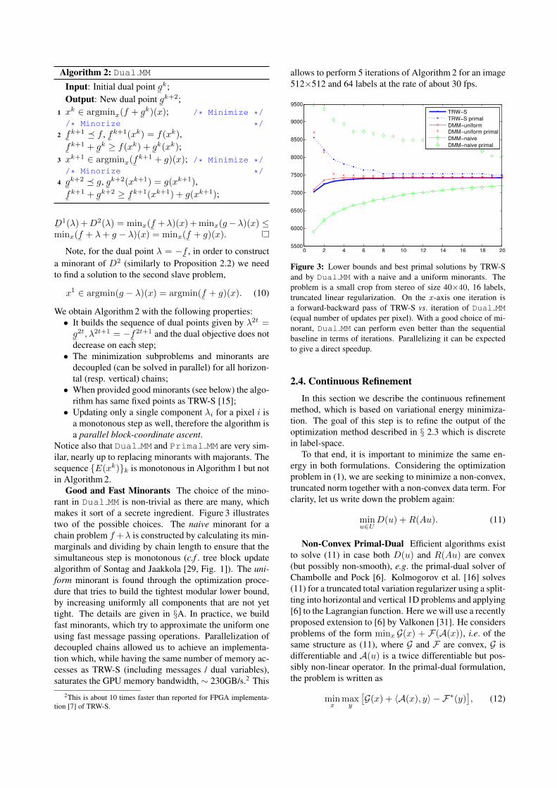
Algorithm 2: Dual MM

Input: Initial dual point¯gk;

Output: New dual point¯gk+2;

1 xk ∈ argminx(f +¯gk)(x); /* Minimize */

/* Minorize */

2¯fk+1 � f ,

¯fk+1(xk) = f(xk),

¯fk+1 +

¯gk ≥ f(xk) +

¯gk(xk);

3 xk+1 ∈ argminx(¯fk+1 + g)(x); /* Minimize */

/* Minorize */

4¯gk+2 � g,

¯gk+2(xk+1) = g(xk+1),

¯fk+1 +

¯gk+2 ≥

¯fk+1(xk+1) + g(xk+1);

¯D1(λ) +D2(λ) = minx(

¯f +λ)(x) + minx(g−λ)(x) ≤

minx(¯f + λ+ g − λ)(x) = minx(

¯f + g)(x).

Note, for the dual point λ = −¯f , in order to construct

a minorant of D2 (similarly to Proposition 2.2) we needto find a solution to the second slave problem,

x1 ∈ argmin(g − λ)(x) = argmin(¯f + g)(x). (10)

We obtain Algorithm 2 with the following properties:• It builds the sequence of dual points given by λ2t =

¯g2t, λ2t+1 = −

¯f2t+1 and the dual objective does not

decrease on each step;• The minimization subproblems and minorants are

decoupled (can be solved in parallel) for all horizon-tal (resp. vertical) chains;

• When provided good minorants (see below) the algo-rithm has same fixed points as TRW-S [15];

• Updating only a single component λi for a pixel i isa monotonous step as well, therefore the algorithm isa parallel block-coordinate ascent.

Notice also that Dual MM and Primal MM are very sim-ilar, nearly up to replacing minorants with majorants. Thesequence {E(xk)}k is monotonous in Algorithm 1 but notin Algorithm 2.

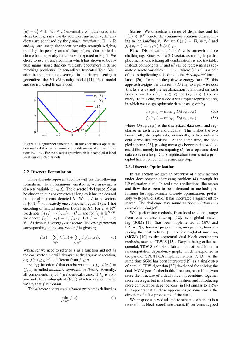
Good and Fast Minorants The choice of the mino-rant in Dual MM is non-trivial as there are many, whichmakes it sort of a secrete ingredient. Figure 3 illustratestwo of the possible choices. The naive minorant for achain problem f +λ is constructed by calculating its min-marginals and dividing by chain length to ensure that thesimultaneous step is monotonous (c.f . tree block updatealgorithm of Sontag and Jaakkola [29, Fig. 1]). The uni-form minorant is found through the optimization proce-dure that tries to build the tightest modular lower bound,by increasing uniformly all components that are not yettight. The details are given in §A. In practice, we buildfast minorants, which try to approximate the uniform oneusing fast message passing operations. Parallelization ofdecoupled chains allowed us to achieve an implementa-tion which, while having the same number of memory ac-cesses as TRW-S (including messages / dual variables),saturates the GPU memory bandwidth, ∼ 230GB/s.2 This

2This is about 10 times faster than reported for FPGA implementa-tion [7] of TRW-S.

allows to perform 5 iterations of Algorithm 2 for an image512×512 and 64 labels at the rate of about 30 fps.

0 2 4 6 8 10 12 14 16 18 205500

6000

6500

7000

7500

8000

8500

9000

9500

TRW−S

TRW−S primal

DMM−uniformDMM−uniform primal

DMM−naive

DMM−naive primal

Figure 3: Lower bounds and best primal solutions by TRW-Sand by Dual MM with a naive and a uniform minorants. Theproblem is a small crop from stereo of size 40×40, 16 labels,truncated linear regularization. On the x-axis one iteration isa forward-backward pass of TRW-S vs. iteration of Dual MM(equal number of updates per pixel). With a good choice of mi-norant, Dual MM can perform even better than the sequentialbaseline in terms of iterations. Parallelizing it can be expectedto give a direct speedup.

2.4. Continuous Refinement

In this section we describe the continuous refinementmethod, which is based on variational energy minimiza-tion. The goal of this step is to refine the output of theoptimization method described in § 2.3 which is discretein label-space.

To that end, it is important to minimize the same en-ergy in both formulations. Considering the optimizationproblem in (1), we are seeking to minimize a non-convex,truncated norm together with a non-convex data term. Forclarity, let us write down the problem again:

minu∈U

D(u) +R(Au). (11)

Non-Convex Primal-Dual Efficient algorithms existto solve (11) in case both D(u) and R(Au) are convex(but possibly non-smooth), e.g. the primal-dual solver ofChambolle and Pock [6]. Kolmogorov et al. [16] solves(11) for a truncated total variation regularizer using a split-ting into horizontal and vertical 1D problems and applying[6] to the Lagrangian function. Here we will use a recentlyproposed extension to [6] by Valkonen [31]. He considersproblems of the form minx G(x) + F(A(x)), i.e. of thesame structure as (11), where G and F are convex, G isdifferentiable and A(u) is a twice differentiable but pos-sibly non-linear operator. In the primal-dual formulation,the problem is written as

minx

maxy

[G(x) + 〈A(x), y〉 − F∗(y)

], (12)

where ∗ is the convex conjugate. Valkonen proposes thefollowing modified primal-dual hybrid gradient method:

xk+1 =(I + τ∂G)−1(xk − τ[∇A(xk)

]Tyk) (13a)

yk+1 =(I + σ∂F∗)−1(yk + σA(2xk+1 − xk)). (13b)

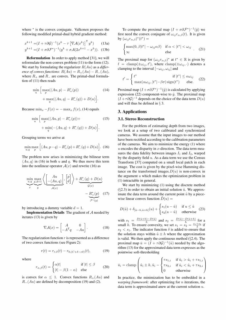
Reformulation In order to apply method [31], we willreformulate the non-convex problem (11) to the form (12).We start by formulating the regularizer R(Au) as a differ-ence of convex functions: R(Au) = R+(Au)−R−(Au),where R+ and R− are convex. The primal-dual formula-tion of (11) then reads

minu

[maxp

(〈Au, p〉 −R∗+(p)) (14)

+ maxq

(〈Au, q〉 −R∗−(q)) +D(u)].

Because minx−f(x) = −maxx f(x), (14) equals

minu

[maxp

(〈Au, p〉 −R∗+(p))+ (15)

+ minq

(−〈Au, q〉+R∗−(q)) +D(u)].

Grouping terms we arrive at

minu,q

maxp

[〈Au, p−q〉−R∗+(p)+R∗−(q)+D(u)

]. (16)

The problem now arises in minimizing the bilinear term〈Au, q〉 in (16) in both u and q. We thus move this terminto the nonlinear operator A(x) and rewrite (16) as

minu,q︸︷︷︸x

maxp,d=1︸ ︷︷ ︸y

⟨[Au

−〈Au, q〉

]︸ ︷︷ ︸A(x)

,

[pd

]⟩+R∗−(q) +D(u)︸ ︷︷ ︸

G(x)

−R∗+(p)︸ ︷︷ ︸F∗(y)

(17)

by introducing a dummy variable d = 1.Implementation Details The gradient ofA needed by

iterates (13) is given by

∇A(x) =

[A 0−ATq −Au

]. (18)

The regularization function r is represented as a differenceof two convex functions (see Figure 2):

r(t) = rε,δ(t)− r0,(C+δ−εδ)(t), (19)

where

rα,β(t) =

{α|t| if |t| ≤ β|t| − β(1− α) else

(20)

is convex for α ≤ 1. Convex functions R+(Au) andR−(Au) are defined by decomposition (19) and (2).

To compute the proximal map (I + σ∂F∗)−1(y) wefirst need the convex conjugate of ωijrα,β(t). It is givenby (ωijrα,β)∗(t∗) ={

max(0, β|t∗| − ωijαβ) if α < |t∗| < ωij

∞ else. (21)

The proximal map for (ωijrα,β)∗ at t∗ ∈ R is given byt = clamp(±ωij , t′), where clamp(±ωij , ·) denotes aclamping to the interval [−ωij , ωij ] and

t′ =

{t∗ if |t∗| ≤ αωijmax(αωij , |t∗|−βσ) sign(t∗) else.

(22)

Proximal map (I+σ∂F∗)−1(y) is calculated by applyingexpression (22) component-wise to y. The proximal map(I+τ∂G)−1 depends on the choice of the data termD(u)and will thus be defined in § 3.

3. Applications3.1. Stereo Reconstruction

For the problem of estimating depth from two images,we look at a setup of two calibrated and synchronizedcameras. We assume that the input images to our methodhave been rectified according to the calibration parametersof the cameras. We aim to minimize the energy (1) whereu encodes the disparity in x-direction. The data term mea-sures the data fidelity between images I1 and I2, warpedby the disparity field u. As a data term we use the CensusTransform [37] computed on a small local patch in eachimage. The cost is given by the pixel-wise Hamming dis-tance on the transformed images.D(u) is non-convex inthe argument u which makes the optimization problem in(1) intractable in general.

We start by minimizing (1) using the discrete method(§2.3) in order to obtain an initial solution u. We approx-imate the data term around the current point u by a piece-wise linear convex function D(u) =

D(u) + δ[u−h,u+h](u) +

{s1(u− u) if u ≤ us2(u− u) otherwise

(23)

with s1 = D(u+h)−D(u)h and s2 = D(u)−D(u+h)

h for asmall h. To ensure convexity, we set s1 = s2 = s1+s2

2 ifs2 < s1. The indicator function δ is added to ensure thatthe solution stays within u ± h where the approximationis valid. We then apply the continuous method (§2.4). Theproximal map u = (I + τ∂G)−1(u) needed by the algo-rithm (13) for the approximated data term expresses as thepointwise soft-thresholding

ui = clamp

ui ± h, ui −τs1,i if ui > ui + τs1,i

τs2,i if ui < ui + τs2,i

0 otherwise

In practice, the minimization has to be embedded in awarping framework: after optimizing for n iterations, thedata term is approximated anew at the current solution u.

3.2. Optical Flow

The optical flow problem for two images I1, I2 is posedagain as model (1). In contrast to stereo estimation, wenow have ui ∈ R2 encoding the flow vector. For thediscrete optimization step (§2.3) the flow problem is de-coupled into two independent stereo-like problems as dis-cussed in §2.2.

For the continuous refinement step, the main prob-lem is again the non-convexity of the data term. In-stead of a convex approximation with two linear slopeswe build a quadratic approximation, now in 2D, follow-ing [34]. The approximated data term reads Di(ui) =δ[ui−h,ui+h](ui)+

Di(ui) +LTi (ui − ui) +

1

2(ui − ui)TQi(ui − ui), (24)

where Li ∈ R2 and Qi ∈ R2×2 are finite difference ap-proximations of the gradient and the Hessian with step-size h. Convexity of (24) is ensured by retaining onlypositive-semidefinite part of Qi as in [34]. The proximalmap u = (I + τ∂G)−1(u) for data term (24) is givenpoint-wise by

uki = clamp

(uki ± h,

uki + τ(Qiui − Li)k1 + τLki

). (25)

Optimizing (1) is then performed as proposed in §2.4.

4. Experiments4.1. Stereo Reconstruction

We evaluate our proposed real-time stereo method ondatasets where Ground-Truth data is available as well ason images captured using a commercially available stereocamera.

4.1.1 Influence of Truncated Regularizer

We begin by comparing the proposed method to a sim-plified version that does not use a truncated norm as reg-ularizer but a standard Total Variation. We show the ef-fect of this change in Fig. 4, where one can observe muchsharper edges, when using a robust norm in the regulariza-tion term. On the downside it is more sensitive to outliers,which however can be removed in a post-processing steplike a two-side consistency check.

4.1.2 Live Dense Reconstruction

To show the performance of our stereo matching methodin a real live setting, we look at the task of creating alive dense reconstruction from a set of depth images. Tothat end, we are using a reimplementation of KinectFusionproposed by Newcombe et al. [20] together with the out-put of our method. This method was originally designedto be used with the RGBD output of a Microsoft Kinectand tracks the 6 DOF position of the camera in real-time.

(a) Input (b) Groundtruth

(c) TV regularization (d) Proposed Method

Figure 4: Influence of the robust regularizer in the continuousrefinement on stereo reconstruction quality.

(a) Refinement (b) No Refinement

Figure 5: Influence of continuous refinement on the reconstruc-tion quality of KinectFusion.

For the purpose of this experiment we replace the Kinectwith a Point Grey Bumblebee2 stereo camera. KinectFu-sion can only handle relatively small camera movementsbetween images, so a high framerate is essential. We setthe parameters to our method to achieve a compromisebetween highest quality and a framerate of ≈ 4 − 5 fps:camera resolution 640× 480, 128 disparities, 4 iterationsof Dual MM, 5 warps and 40 iterations per warp of thecontinuous refinement.

Influence of Continuous Refinement The first stageof our reconstruction method, Dual MM, already delivershigh quality disparity images that include details on finestructures and depth discontinuities that are nicely alignedwith edges in the image. In this experiment we want toshow the influence of the second stage, the continuous re-finement, on the reconstruction quality of KinectFusion.To that end we mount the camera on a tripod and collect300 depthmaps live from our full method and 300 frameswith the continuous refinement switched off. By switch-ing off the camera tracking, the final reconstruction willshow us the artifacts produced by the stereo method. Fig-ure 5 depicts the result of this comparison. One can easilysee that the output of the discrete method contains fine de-tails, but suffers from staircasing artifacts on slanted sur-faces due to the integer solution. The increase in qual-ity due to the refinement stage can be especially seen onfar away objects, where a disparity step of 1 pixel is notenough to capture smooth surfaces.

Timing To show the influence of the individual stepsin our stereo method on runtime, we break down the total

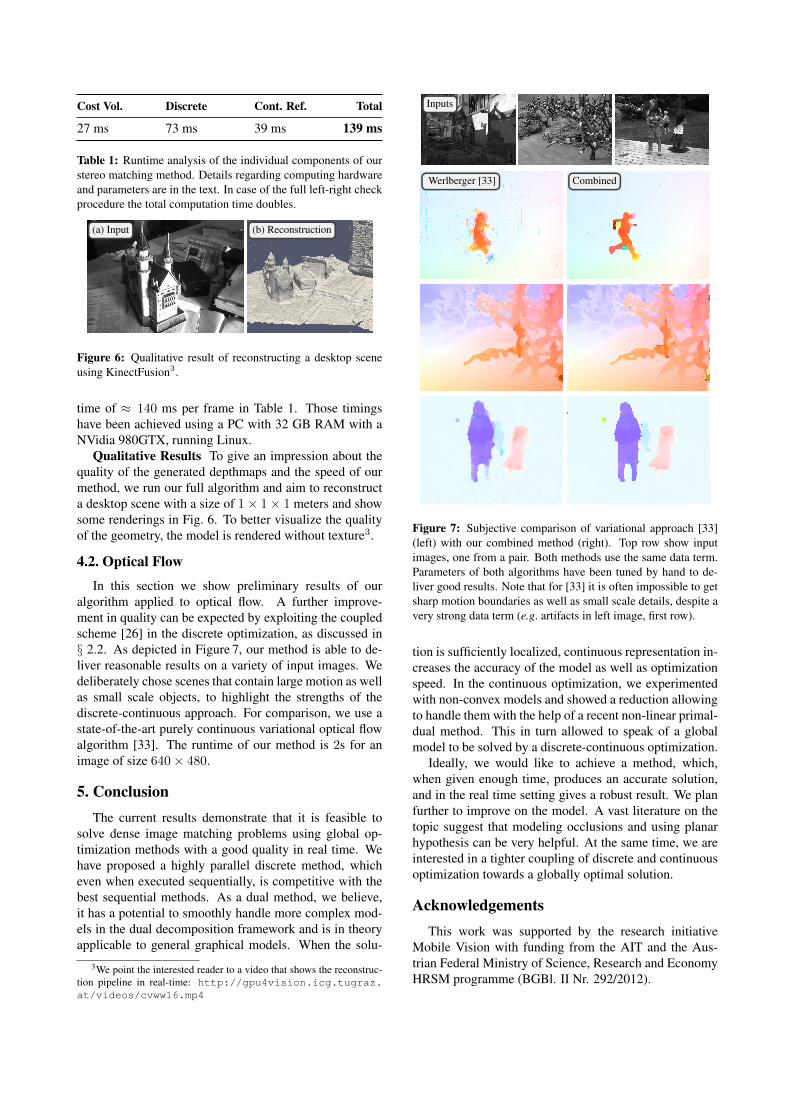
Cost Vol. Discrete Cont. Ref. Total

27 ms 73 ms 39 ms 139 ms

Table 1: Runtime analysis of the individual components of ourstereo matching method. Details regarding computing hardwareand parameters are in the text. In case of the full left-right checkprocedure the total computation time doubles.

(a) Input (b) Reconstruction

Figure 6: Qualitative result of reconstructing a desktop sceneusing KinectFusion3.

time of ≈ 140 ms per frame in Table 1. Those timingshave been achieved using a PC with 32 GB RAM with aNVidia 980GTX, running Linux.

Qualitative Results To give an impression about thequality of the generated depthmaps and the speed of ourmethod, we run our full algorithm and aim to reconstructa desktop scene with a size of 1× 1× 1 meters and showsome renderings in Fig. 6. To better visualize the qualityof the geometry, the model is rendered without texture3.

4.2. Optical Flow

In this section we show preliminary results of ouralgorithm applied to optical flow. A further improve-ment in quality can be expected by exploiting the coupledscheme [26] in the discrete optimization, as discussed in§ 2.2. As depicted in Figure 7, our method is able to de-liver reasonable results on a variety of input images. Wedeliberately chose scenes that contain large motion as wellas small scale objects, to highlight the strengths of thediscrete-continuous approach. For comparison, we use astate-of-the-art purely continuous variational optical flowalgorithm [33]. The runtime of our method is 2s for animage of size 640× 480.

5. ConclusionThe current results demonstrate that it is feasible to

solve dense image matching problems using global op-timization methods with a good quality in real time. Wehave proposed a highly parallel discrete method, whicheven when executed sequentially, is competitive with thebest sequential methods. As a dual method, we believe,it has a potential to smoothly handle more complex mod-els in the dual decomposition framework and is in theoryapplicable to general graphical models. When the solu-

3We point the interested reader to a video that shows the reconstruc-tion pipeline in real-time: http://gpu4vision.icg.tugraz.at/videos/cvww16.mp4

Inputs

Werlberger [33] Combined

Figure 7: Subjective comparison of variational approach [33](left) with our combined method (right). Top row show inputimages, one from a pair. Both methods use the same data term.Parameters of both algorithms have been tuned by hand to de-liver good results. Note that for [33] it is often impossible to getsharp motion boundaries as well as small scale details, despite avery strong data term (e.g. artifacts in left image, first row).

tion is sufficiently localized, continuous representation in-creases the accuracy of the model as well as optimizationspeed. In the continuous optimization, we experimentedwith non-convex models and showed a reduction allowingto handle them with the help of a recent non-linear primal-dual method. This in turn allowed to speak of a globalmodel to be solved by a discrete-continuous optimization.

Ideally, we would like to achieve a method, which,when given enough time, produces an accurate solution,and in the real time setting gives a robust result. We planfurther to improve on the model. A vast literature on thetopic suggest that modeling occlusions and using planarhypothesis can be very helpful. At the same time, we areinterested in a tighter coupling of discrete and continuousoptimization towards a globally optimal solution.

AcknowledgementsThis work was supported by the research initiative

Mobile Vision with funding from the AIT and the Aus-trian Federal Ministry of Science, Research and EconomyHRSM programme (BGBl. II Nr. 292/2012).

References[1] Arashloo, S. R. and Kittler, J. (2014). Fast pose invariant

face recognition using super coupled multiresolution Markovrandom fields on a GPU. Pattern Recognition Letters, 48.

[2] Banz, C., Hesselbarth, S., Flatt, H., Blume, H., and Pirsch,P. (2010). Real-time stereo vision system using semi-globalmatching disparity estimation: Architecture and FPGA-implementation. In ICSAMOS.

[3] Bleyer, M. and Gelautz, M. (2008). Simple but effective treestructures for dynamic programming-based stereo matching.In VISAPP.

[4] Brox, T., Bruhn, A., Papenberg, N., and Weickert, J. (2004).High accuracy optical flow estimation based on a theory forwarping. In ECCV.

[5] Brox, T., Bruhn, A., and Weickert, J. (2006). Variationalmotion segmentation with level sets. In ECCV, volume 3951.

[6] Chambolle, A. and Pock, T. (2011). A first-order primal-dual algorithm for convex problems with applications toimaging. Journal of Mathematical Imaging and Vision, 40(1).

[7] Choi, J. and Rutenbar, R. A. (2012). Hardware implementa-tion of MRF MAP inference on an FPGA platform. In FieldProgrammable Logic.

[8] Combettes, P. L. and Pesquet, J.-C. (2011). Proximal split-ting methods in signal processing. In Fixed-Point Algorithmsfor Inverse Problems in Science and Engineering.

[9] Drory, A., Haubold, C., Avidan, S., and Hamprecht, F.(2014). Semi-global matching: A principled derivation interms of message passing. In Pattern Recognition, volume8753.

[10] Facciolo, G., de Franchis, C., and Meinhardt, E. (2015).MGM: A significantly more global matching for stereovision.In BMVC.

[11] Hirschmuller, H. (2011). Semi-global matching-motivation, developments and applications.

[12] Hosni, A., Rhemann, C., Bleyer, M., Rother, C., andGelautz, M. (2013). Fast cost-volume filtering for visual cor-respondence and beyond. PAMI, 35(2).

[13] Hurkat, S., Choi, J., Nurvitadhi, E., Martınez, J. F., andRutenbar, R. A. (2012). Fast hierarchical implementation ofsequential tree-reweighted belief propagation for probabilis-tic inference. In Field Programmable Logic.

[14] Kappes, J. H., Andres, B., Hamprecht, F. A., Schnorr, C.,Nowozin, S., Batra, D., Kim, S., Kausler, B. X., Lellmann, J.,Komodakis, N., and Rother, C. (2013). A comparative studyof modern inference techniques for discrete energy minimiza-tion problem. In CVPR.

[15] Kolmogorov, V. (2006). Convergent tree-reweighted mes-sage passing for energy minimization. PAMI, 28(10).

[16] Kolmogorov, V., Pock, T., and Rolinek, M. (2015). Totalvariation on a tree. CoRR, abs/1502.07770.

[17] Lawler, E. (1966). Optimal cycles in doubly weighted di-rected linear graphs. In Intl Symp. Theory of Graphs.

[18] Menze, M., Heipke, C., and Geiger, A. (2015). Discreteoptimization for optical flow. In GCPR.

[19] Narasimhan, M. and Bilmes, J. (2005). A supermodular-submodular procedure with applications to discriminativestructure learning. In Uncertainty in Artificial Intelligence.

[20] Newcombe, R. A., Izadi, S., Hilliges, O., Molyneaux, D.,Kim, D., Davison, A. J., Kohli, P., Shotton, J., Hodges, S.,and Fitzgibbon, A. (2011). Kinectfusion: Real-time densesurface mapping and tracking. In ISMAR.

[21] Ochs, P., Chen, Y., Brox, T., and Pock, T. (2014). ip-iano: Inertial proximal algorithm for non-convex optimiza-tion. SIAM JIS, 7(2).

[22] Prusa, D. and Werner, T. (2015). Universality of the localmarginal polytope. PAMI, 37(4).

[23] Ranftl, R., Bredies, K., and Pock, T. (2014). Non-localtotal generalized variation for optical flow estimation. InECCV.

[24] Ranftl, R., Gehrig, S., Pock, T., and Bischof, H. (2012).Pushing the limits of stereo using variational stereo estima-tion. In Intelligent Vehicles Symposium.

[25] Roth, S., Lempitsky, V., and Rother, C. (2009). Discrete-continuous optimization for optical flow estimation. In Statis-tical and Geometrical Approaches to Visual Motion Analysis,volume 5604.

[26] Shekhovtsov, A., Kovtun, I., and Hlavac, V. (2008). Effi-cient MRF deformation model for non-rigid image matching.CVIU, 112.

[27] Shekhovtsov, A., Swoboda, P., and Savchynskyy, B.(2015). Maximum persistency via iterative relaxed inferencewith graphical models. In CVPR.

[28] Sinha, S. N., Scharstein, D., and Szeliski, R. (2014).Efficient high-resolution stereo matching using local planesweeps. In CVPR.

[29] Sontag, D. and Jaakkola, T. S. (2009). Tree block coordi-nate descent for MAP in graphical models. In AISTATS.

[30] Taniai, T., Matsushita, Y., and Naemura, T. (2014). Graphcut based continuous stereo matching using locally shared la-bels. In CVPR.

[31] Valkonen, T. (2014). A primal-dual hybrid gradient methodfor nonlinear operators with applications to MRI. InverseProblems, 30(5).

[32] Wainwright, M., Jaakkola, T., and Willsky, A. (2005).MAP estimation via agreement on (hyper)trees: Message-passing and linear-programming approaches. IEEE Trans-actions on Information Theory, 51(11).

[33] Werlberger, M. (2012). Convex Approaches for High Per-formance Video Processing. PhD thesis, Institute for Com-puter Graphics and Vision, Graz University of Technology,Graz, Austria.

[34] Werlberger, M., Pock, T., and Bischof, H. (2010). Motionestimation with non-local total variation regularization. InCVPR.

[35] Werner, T. (2007). A linear programming approach to max-sum problem: A review. PAMI, 29(7).

[36] Woodford, O., Torr, P., Reid, I., and Fitzgibbon, A. (2009).Global stereo reconstruction under second-order smoothnesspriors. PAMI, 31(12).

[37] Zabih, R. and Woodfill, J. (1994). Non-parametric localtransforms for computing visual correspondence. In ECCV,volume 801.

Appendix A. Details of Dual MMIn this section we specify details regarding computa-

tion of minorants in Dual MM. The minorants are com-puted using message passing and we’ll also need the no-tion of min-marginals.

A.1. Min-Marginals and Message Passing

Definition A.1. For cost vector f its min-marginal atnode i is the function mf : L → R given by

mf (xi) = minxV\i

f(x). (26)

Function mf (xi) is a min projection of f(x) onto xionly. Given the choice of xi, it returns the cost of the bestlabeling in f that passes through xi. For a chain problemit can be computed using dynamic programming. Let usassume that the nodes V are enumerated in the order ofthe chain and E = {(i, i+ 1) | i = 1 . . . |V| − 1}. We thenneed to compute: left min-marginals: ϕi−1,i(xi) :=

minx1,...i−1

∑i′<i

fi′(xi′) +∑

i′j′∈E | i′<ifi′j′(xi′ , xj′); (27)

and right min-marginals: ϕi+1,i(xi) :=

minxi+1,...|V |

∑i′>i

fi′(xi′) +∑

i′j′∈E | i′≥ifi′j′(xi′ , xj′). (28)

These values for all ij ∈ E , xi, xj ∈ L can be computeddynamically (recursively). After that, the min-marginalmf (xi) expresses as

mf (xi) = fi(xi) + ϕi−1,i(xi) + ϕi+1,i(xi). (29)

TRW-S method [15] can be derived as selecting onenode i at a time and maximizing (8) with respect to λionly. For the two slave problems in (8) TRW-S needsto compute min-marginals mf+λ(xi) and mg−λ(xi). A(non-unique) optimal choice for λi would be to ensure that

mf+λ(xi) = mg−λ(xi) ∀xi ∈ L (30)

by setting

λi := λi + (mg−λ(xi)−mf+λ(xi))/2. (31)

If i and j are two nodes in a chain f+λ then performingthe update of λi changes the min-marginal at j and vice-versa. The updates must be implemented sequentially orotherwise one gets a non-monotonous behavior and themethod may fail to converge (see [15]).

TRW-S gains its efficiency in that after the update (31),the min-marginal at a neighboring node can be recom-puted by a single step of dynamic programming. Let theneighboring node be j = i + 1. The expression for theright min-marginal at j remains correct and the expres-sion for left min-marginal is updated using its recurrentexpression ϕij(xj) :=

minxi

[ϕi−1,i(xi) + fi(xi) + fij(xi, xj)

], (32)

also known as message passing. Then min-marginal at jbecomes available through (29).

It is possible to perform update (31) in parallel by scal-ing down the step size by the number of variables (orthe length of the chain). This is equivalent to decom-posing a chain f into n copies with costs f/n so thatthey contribute one for each node i with a min-marginalmf (xi)/n. Confer to the parallel tree block update algo-rithm of Sontag and Jaakkola [29, Fig. 1]). However, thegain from the palatalization does not pay off the decreasein the step size.

A.2. Slacks

In the following we will also use the term slack.Shortly, it is explained as follows. The dual problem (8)can be written as a linear program, see e.g., [35]. Dual in-equality constraints in that program can satisfied as equal-ities, in which case they are tight, or they can be satisfiedas strict inequalities in which case there is a slack. Equiv-alent reparametrization of the problem (change of the dualvariables) can propagate a slack from one constraint (cor-responding to a label-node pair) to another one. If allconstraints in a group becomes non-tight, their minimumslack can be subtracted and increments the lower bound.Since for a chain problem the LP relaxation is tight, themaximum slack that can be concentrated in a label-nodeequals the corresponding min-marginal.

A.3. Good Minoratns

Definition A.2. A modular minorant λ of f is maximalif there is no other modular minorant λ′ ≥ λ such thatλ′(x) > λ(x) for some x.

Lemma A.3. For a maximal minorant λ of f all min-marginals of f − λ are identically zero.

Proof. Since λ is a minorant, min-marginals mi(xi) =minxV\i [f(x)− λ(x)] are non-negative. Assume for con-tradiction that ∃i, ∃xi such that mi(xi) > 0. Clearly,λ′(x) := λ(x) + mi(xi) is also a minorant and λ′ >λ.

Even using maximal minorants, the Algorithm 2 canget stuck in fixed points which do not satisfy weak tree

agreement [15], e.g. suboptimal even in the class of mes-sage passing algorithms. Consider the following exampleof a minorant leading to a poor fixed point.

Example A.4. Consider a model in Figure 8 with two la-bels and strong Ising interactions ensuring that the optimallabeling is uniform. If we select minorants that just takesthe unary term, without redistributing it along horizontalor vertical chains, the lower bound will not increase. Forexample, for the horizontal chain (v1, v2), the minorant(1, 0) (displayed values correspond to λv(1) − λv(2)).This minorant is maximal, but it does not propagate theinformation available in v1 to v2 for the exchange withthe vertical chain (v2, v4).

+0.5

+1

Figure 8: Example minorize-minimize stucks with a minorantthat does not redistribute slack.

A.3.1 Uniform Minorants

Dual algorithms, by dividing the slacks between subprob-lems ensure that there is always a non-zero fraction of it(depending on the choice of weights in the scheme) prop-agated along each chain. We need a minorant, which willexpose in every variable what is the preferable solutionfor the subproblem. We can even try to treat all variablesuniformly. The practical strategy proposed below is moti-vated by the following.

Proposition A.5. Let f∗ = minx f(x) and let Ou be thesupport set of all optimal solutions x∗u in u ∈ V . Con-sider the minorant λ given by λu(xu) = ε(1 − Ou) andmaximizing ε:

max{ε | (∀x) ε〈1−O, x〉 ≤ f(x)}. (33)

The above minorant assigns cost ε to all labels butthose in the set of optimal solutions. If the optimal so-lution x∗ is unique, it takes the form λ = ε(1 − x∗).This minorant corresponds to the direction of the subgra-dient method and ε determines the step size which ensuresmonotonicity. However it is not maximal. In f − λ therestill remains a lot of slack that can be useful when ex-changing to the other problem. It is possible to considerf − λ again. If we have solved (33), it will necessarilyhave a larger set of optimal solutions. We can search fora maximal ε1 that can be subtracted from all non-optimallabel-nodes in f −λ and so on. The algorithm is specifiedas Algorithm 3.

Algorithm 3: Maximal Uniform Minorant

Input: Chain subproblem f ;Output: Minorant λ;

1 λ := 0;2 while true3 Compute min-marginals m of f − λ;4 if m = 0 then return λ;5 Let O := [[m = 0]], the support set of optimal

solutions of m− λ;6 Find max{ε | (∀x) ε〈1−O, x〉 ≤ (f − λ)(x)};7 Let λ := λ+ ε(1−O);

The optimization problem in Line 6 can be solved us-ing the minimum ratio cycle algorithm of Lawler [17]. Wesearch for a path with a minimum ratio of the cost givenby (f − λ)(x) to the number of selected labels with non-zero min-marginals given by 〈1−O, x〉. This algorithm israther efficient, however Algorithm 3 it is still too costlyand not well-suited for a parallel implementation. We willnot use this method in practice directly, rather it estab-lishes a sound baseline that can be compared to.

The resulting minorant λ is maximal and uniform inthe following sense.

Lemma A.6. Let m be the vector of min-marginals of f .The uniform minorant λ found by Algorithm 3 satisfies

λ ≥ m/n, (34)

where n is the length of the longest chain in f .

Proof. This is ensured by Algorithm 3 as in each step theincrement ε results from dividing the min-marginal by〈1−O, x〉 which is at most the length of the chain.

In fact, when the chain is strongly correlated, the mi-norant will approach m/n and we cannot do better thanthat. However, if the correlation is not as strong the mi-norant becomes tighter, and in the limit of zero pairwiseinteractions there holds λ = m. In a sense the minorantcomputes “decorrellated” min-marginals.

The next example illustrates uniform minorants andsteps of the algorithm.

Example A.7. Consider a chain model with the followingdata unary cost entries (3 labels, 6 nodes):

0 0 1 0 0 89 7 0 3 2 87 3 6 9 1 0

The regularization is a Potts model with costfuv(xu, xv) = 1[[xu 6= xv]]. Min-marginals of theproblem and iteration of Algorithm 3 are ilustrated inFigure 9. At the first iteration the constructed minorant is

0 0 0 0 0 11 1 1 1 1 11 1 1 1 1 0

And the final minorant is:

0 0 0 0 0 78 7 1 2 2 76 4 6 7 1 0

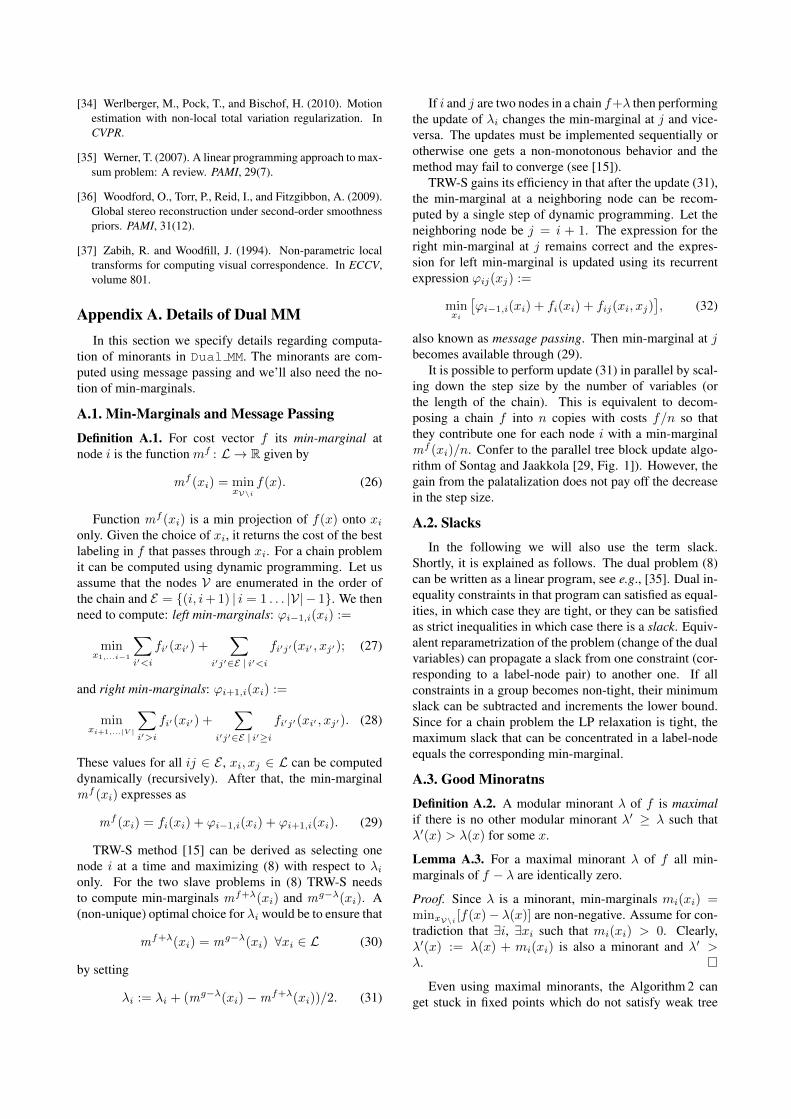
The minorant follows min-marginals (first plot in Fig-ure 9), because the interaction strength is relatively weakand min-marginals are nearly independent. If we in-crease interaction strength to 5, we find the following min-marginals and minorant, respectively:0 0 0 0 0 314 15 8 8 7 812 13 15 10 1 00 0 0 0 0 35.5 5.5 3 3 3 34.75 4.75 4.75 4.75 1 0

It is seen that in this case min-marginals are correlated andonly a fraction can be drained in parallel. The uniformapproach automatically divides the cost equally betweenstrongly correlated labels.

(a)

0

10

8

0

8

5

0

1

7

0

4

10

0

3

1

7

8

0

(b)

0

9

7

0

6

3

0

0

6

0

1

7

0

2

0

6

7

0

(c)

0

8

6

0

5

2

0

0

5

0

0

6

0

0

0

5

5

0

Figure 9: (a) Min-marginals (normalized by subtracting thevalue of the minimum) at vertices and arrows allowing to back-track the optimal solution passing through a given vertex. (b),(c) min-marginals of f −λ after one (resp. two) iterations of Al-gorithm 3 (ε1 = 1 and ε2 = 1). With each iteration the numberof vertices having zero min-marginal strictly increases.

A basic performance test of Dual MM with uniformminorants versus TRW-S is shown in Figure 3. It demon-strates that the Dual MM can be faster, when providedgood minorants. The only problem is that determining theuniform minorant involves repeatedly solving minimumratio path problems, plus there is a numerical instabilityin determining the support set of optimal solutions O.

A.3.2 Iterative Minorants

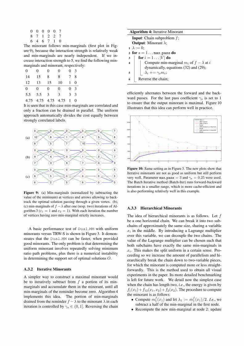
A simpler way to construct a maximal minorant wouldbe to iteratively subtract from f a portion of its min-marginals and accumulate them in the minorant, until allmin-marginals of the reminder become zero. Algorithm 4implements this idea. The portion of min-marginalsdrained from the reminder f −λ to the minorant λ in eachiteration is controlled by γs ∈ (0, 1]. Reversing the chain

Algorithm 4: Iterative Minorant

Input: Chain subproblem f ;Output: Minorant λ;

1 λ := 0;2 for s = 1 . . . max pass do3 for i = 1 . . . |V | do4 Compute min-marginal mi of f − λ at i

dynamically, equations (32) and (29);5 λi += γsmi;

6 Reverse the chain;

efficiently alternates between the forward and the back-ward passes. For the last pass coefficient γs is set to 1to ensure that the output minorant is maximal. Figure 10illustrates that this idea can perform well in practice.

2 3 4 5 6 7 8 9 10

7200

7400

7600

7800

8000

8200

TRW−STRW−S primalDMM−uniformPrimalDMM−Iterative-s−3−frac−0.25PrimalDMM−Batch-Iter−3−frac−0.25Primal

Figure 10: Same setting as in Figure 3. The new plots show thatIterative minorants are not as good as uniform but still performvery well. Parameter max pass = 3 and γs = 0.25 were used.The Batch Iterative method (Batch-Iter) runs forward-backwarditerations in a smaller range, which is more cache-efficient andis also performing relatively well in this example.

A.3.3 Hierarchical Minorants

The idea of hierarchical minorants is as follows. Let fbe a one horizontal chain. We can break it into two sub-chains of approximately the same size, sharing a variablexi in the middle. By introducing a Lagrange multiplierover this variable, we can decouple the two chains. Thevalue of the Lagrange multiplier can be chosen such thatboth subchains have exactly the same min-marginals inxi. This makes the split uniform in a certain sense. Pro-ceeding so we increase the amount of parallelism and hi-erarchically break the chain down to two-variable pieces,for which the minorant is computed more or less straight-forwardly. This is the method used to obtain all visualexperiments in the paper. Its more detailed benchmarkingis left for future work. We detail now the simplest casewhen the chain has length two, i.e., the energy is given byf1(x1)+f12(x1, x2)+f2(x2). The procedure to computethe minorant is as follows:• Compute mf

1 (x1) and let λ1 := mf1 (x1)/2. I.e., we

subtract a half of the min-marginal in the first node.• Recompute the new min-marginal at node 2: update

Algorithm 5: HandshakeInput: Energy terms fi, fj , fij , messages ϕi−1,i(xi)

and ϕj,j+1(xj) ;Output: Messages for decorrellated chains: ϕji(xi)

and ϕij(xj) ;/* Message from j to i */

1 ϕji(xi) := Msgji(fj + ϕj,j+1);/* Total min-marginal at i */

2 mi(xi) := ϕi−1,i(xi) + fi(xi) + ϕji(xi);/* Share a half to the right */

3 ϕij(xj) := Msgij(mi/2− ϕji);/* Bounce back what cannot be shared */

4 ϕji(xi) := Msgji(−ϕij);5 Procedure Msgij(a)

Input: Unary cost a ∈ RK ;Output: Message from i to j;

6 return ϕ(xj) := minxi∈L[a(xi) + fij(xi, xj)

];

the message ϕ12(x2) := Msg12(f1 − λ1); Reassem-ble mf−λ

2 (x2) = ϕ12(x2) + f2(x2).• Take this whole remaining min-marginal to the mi-

norant: let λ2 := mf−λ2 (x2).

• Recompute the new min-marginal at node 1: updatethe message ϕ21(x1) := Msg21(f2−λ2); It still maybe non-zero. For example, if the pairwise term of fis zero we recover the remaining half of the initialmin-marginal at node 1. Let λ1 += mf−λ

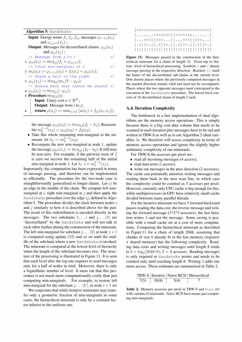
1 (x1).Importantly, the computation has been expressed in termsof message passing, and therefore can be implementedas efficiently. The procedure fro the two-node case isstraightforwardly generalized to longer chains. Let ij bean edge in the middle of the chain. We compute left min-marginal at i, right min-marginal at j and then apply theHandshake procedure over the edge ij, defined in Algo-rithm 5. The procedure divides the slack between nodes iand j similarly to how it is described above for the pair.The result of this redistribution is encoded directly in themessages. The two subchains 1, . . . i and j, . . . |V| are“decorrellated” by the Handshake and will not talk toeach other further during the construction of the minorant.The left min-marginal for subchain j, . . . |V| at node j+ 1is computed using update (32) and so on until the mid-dle of the subchain where a new Handshake is invoked.The minorant is computed at the lowest level of hierarchywhen the length of the subchain becomes two. The struc-ture of the processing is illustrated in Figure 11. It is seenthat each level after the top one requires to send messagesonly for a half of nodes in total. Moreover, there is onlya logarithmic number of level. It turns out that this pro-cedure is not much more computationally costly than justcomputing min-marginals. For example, to restore leftmin-marginal for the subchain j, . . . |V |, in node i+ 1 we

We conjecture that while iterative minorants may trans-fer only a geometric fraction of min-marginals in somecases, the hierarchical minorant is only by a constant fac-tor inferior to the uniform one.

[>>>>>>>>>>>>>>><<<<<<<<<<<<<<<][.......<<<<<<<][>>>>>>>.......][...<<<][>>>...][...<<<][>>>...][.<][>.][.<][>.][.<][>.][.<][>.][][][][][][][][][][][][][][][][]

Figure 11: Messages passed in the construction of the hier-archical minorant for a chain of length 32. From top to bot-tom: level of hierarchical processing. Symbols > and < denotemessage passing in the respective direction. Brackets [] markthe limits of the decorrellated sub-chains at the current level.Dots denote places where the previously computed messages inthe needed direction remain valid and need not be recomputed.Places where the two opposite messages meet correspond to theexecution of the Handshake procedure. The lowest level con-sists of 16 decorrellated chains of length 2 each.

A.4. Iteration Complexity

The bottleneck in a fast implementation of dual algo-rithms are the memory access operations. This is simplybecause there is a big cost data volume that needs to bescanned in each iteration plus messages have to be red andwritten in TRW-S as well as in out Algorithm 2 (dual vari-ables λ). We therefore will assess complexity in terms ofmemory access operations and ignore the slightly higherarithmetic complexity of our minorants.

For TRW-S the accesses per pixel are:• read all incoming messages (4 access);• read data term (1 access);• write out messages in the pass direction (2 accesses).

The cache can potentially amortize writing messages andreading them back in the next scan line, in which casethe complexity could be counted as 5 accesses per pixel.However, currently only CPU cache is big enough for this,while multiprocessors in GPU have relatively small cachedivided between many parallel threads.

For the iterative minorant we have 3 forward-backwardpasses reading the data cost, the reverse message and writ-ing the forward message (3*2*3 accesses), the last itera-tion writes λ and not the message. Some saving is pos-sible with a small cache set at a cost of more computa-tions. Computing the hierarchical minorant as describedin Figure 11 for a chain of length 2048, assuming thatchunks of size 8 already fit in the fast memory (registers+ shared memory) has the following complexity. Read-ing data costs and writing messages until length 8 totalsto 2 + log2(2048/8)/2 = 6 accesses. Reading messagesis only required at Handshake points and needs to becounted only until reaching length 8. Writing λ adds onemore access. These estimates are summarized in Table 2.

TRW-S Iterative Naive BCD Hierarchical7(5) 18(8) 5(4) 7

Table 2: Memory accesses per pixel in TRW-S and Dual MMwith variants of minorants. Naive BCD here means just comput-ing min-marginals.