Scholars' Mine Scholars' Mine

Masters Theses Student Theses and Dissertations

1965

Matching of a horn antenna to its dense surrounding media by the Matching of a horn antenna to its dense surrounding media by the

use of artificial dielectric methods use of artificial dielectric methods

Paul Arthur Ray

Follow this and additional works at: https://scholarsmine.mst.edu/masters_theses

Part of the Electrical and Computer Engineering Commons

Department: Department:

Recommended Citation Recommended Citation Ray, Paul Arthur, "Matching of a horn antenna to its dense surrounding media by the use of artificial dielectric methods" (1965). Masters Theses. 5202. https://scholarsmine.mst.edu/masters_theses/5202

This thesis is brought to you by Scholars' Mine, a service of the Missouri S&T Library and Learning Resources. This work is protected by U. S. Copyright Law. Unauthorized use including reproduction for redistribution requires the permission of the copyright holder. For more information, please contact scholarsmine@mst.edu.

MATCHING OF A HORN ANTENNA TO ITS DENSE SURROUNDING MEDIA BY THE USE OF ARTIFICIAL DIELECTRIC METHODS

BY~ PAUL A. RAY J l1t.J)

A

THESIS

submitted to the faculty of the

UNIVERSITY OF MISSOURI AT ROLLA

in partial fulfilLment of the requirements for the

Degree of

MASTER OF SCIENCE IN ELECTRICAL ENGINEERING

Rolla, Missouri

1965

115t&q

~ , Approved by

~(advisor) d?. t. otr~ ~ R 8~ ~4! tJa&~

ABSTRACT

The purpose of this thesis is to design an artificial

dielectric slug to match a horn in a media such as water

and to discuss a method of determining experimentally its

dielectric properties.

The design is based on known artificial dielectric

methods. The method of determining the dielectric proper­

ties is by microwave waveguide reflection techniques.

This thesis deals with the theoretical aspects and

suggests an experimental method of determining the practi­

cability of such a matching method.

ii

ACKNOWLEDGEMENTS

The author wishes to acknowledge the special assist­

ance given to him by his advisor, Gabriel G. Sketek,

Professor of Electrical Engineering at the University of

Missouri at Rolla.

The author is also indebted to Frank Huskey of the

Electrical Machine Shop for his help in constructing the

experimental equipment.

iii

TABLE OF CONTENTS

ABSTRACT • . • • • • . . . . . . . . ACKNOWLEDGEMENTS . • . . . • LIST OF SYMBOLS . • . • • • LIST OF FIGURES

. . . . I.

II.

INTRODUCTION . .

REVIEW OF THE LITERATURE .

A.

B.

Literature Concerning Artificial Dielectrics • . • • • • . . . • . • . Literature Cencerning Measurement of Dielectric Properties • • . • . . • .

III. DESIGN OF AN ARTIFICIAL DIELECTRIC SLUG

A.

. .

. . . . . .

. . .

B. c.

Introduction • . • • • • . • • Theoretical Analysis • . • • • Experimental Design of Slug to Placed ~n the Horn Antenna • •

. . . . . . . . be . . . .

IV. DISCUSSION OF THE MEASUREMENT OF DIELECTRIC

iv

:page

ii iii

v vi

1

3

3

3

5

5 8

14

PROPERTIES • . . • . • • . • . . . 20

A. Introduction • . • • • . • • • B. c.

Theoretical Analysis • . • . • Procedure for Measuring the Dielectric Properties • • • . • •

V. CONCLUSIONS . . . . . . APPENDIX . • . . . . . . • . . BIBLIOGRAPHY • • • . . . • . VITA • • • . • •

. . . . . . 20 20

37

41

43 45 47

Symbol

E, H

E p

E e

E. ~

E pa' E ea'

p

p

e:

1l ..

e:g, llo

a.

r

t

y

n

cr

w

A.g, A.o, A.l

z X

E. ~a

v

LIST OF SYMBOLS

Analytical or Physical Meaning of Symbol

General vector electric and magnetic field strength respectively.

Dipole field produced by all obstacles in the array.

Effective field acting to polarize the obstacle at the origin.

Interaction field.

Fields averaged over the volume of a unit cell (abc).

Average dipole polarization vector.

Dipole moment vector.

Permittivity.

Permeability.

Permittivity and permeability of free space.

Polarizability constant.

Reflection coefficient.

Transmission coefficient.

Propagation constant.

Intrinsic impedance.

Conductivity.

Radian frequency.

Waveguide, free space, and region 1 wavelength respectively.

Wave impedance in x direction.

LIST OF FIGURES

Figure No.

1. Artificial Dielectric Structure .• ~ . . . . 2. Three-dimensional Artificial Dielectric .

3. Lattice Structure . . . . . . . . . . . . . . . . 4. Top View and Side View of Antenna • . . . . . . . 5.

6.

Top View of Antenna • • . . . . Cross-sectional View of Antenna •

7. Cross-section with Numbers . . 8. Graph of E versus N • • • • . . . . . . . 9. ~Transmitting-and Receiving Systems

10. Angle Conditions at Boundary

11. Formation of Standing Waves . •

12. Wave ReBleotion on a Dielectric Layer

13. Arrangement for Measuring a Dielectric 2

14. Block Diagram of Equipment to be used in the Laboratory . . . . . . . . . . . . . . . . .

15. Standing Wave Pattern in Slotted Section . . 16. Square Law Measurements . • • . • • • • •

vi

Page

8

10

13

15

16

16

17

18

18

21

23

28

31

38

39

40

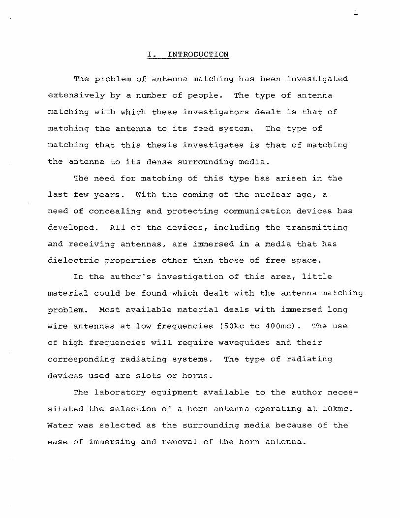
I. INTRODUCTION

The problem of antenna matching has been investigated

extensively by a number of people. The type of antenna

matching with wmich these investigators dealt is that of

matching the antenna to its feed system. The type of

matching that this thesis investigates is that of matching

the antenna to its dense surrounding media.

The need for matching of this type has arisen in the

last few years. With the coming of the nuclear age, a

need of concealing and protecting communication devices has

developed. All of the devices, including the transmitting

and receiving antennas, are immersed in a media that has

dielectric properties other than those of free space.

1

In the author's investigation of this area, little

material could be found which dealt with the antenna matching

problem. Most available material deals with immersed long

wire antennas at low frequencies (SOkc to 400rnc) . The use

of high frequencies will require waveguides and their

corresponding radiating systems. The type of radiating

devices used are slots or horns.

The laboratory equipment available to the author neces­

sitated the selection of a horn antenna operating at lOkmc.

Water was selected as the surrounding media because of the

ease of immersing and removal of the horn antenna.

The purpose of this thesis is to design a device that

will match a horn antenna to its surrounding media. The

procedure for determining the properties of this device

will also be discussed.

2

3

II. REVIEW OF THE LITERATURE

Literature Concerning Artificial Dielectrics

The subject of artificial dielectrics had its beginning

in the mid 1940's. Kock(l), in the period 1944-1948, sug­

gested the use of artificial dielectrics to replace the

actual dielectric in order to overcome their major disadvan­

tage. This disadvantage is the vast weight and mass of

solid dielectrics.

In the following years, various authors contributed to

this area; those who performed the major work are Carlson

and Heins(2) in 1947, Brown(3) in 1950, Cohn(4) in 1949,

Susskind(5) in 1952, and El-Kharadly and Jackson(6) in

1953. The reference, upon which most of the first part of

this thesis is based, is by Collin(?).

Literature Concerning Measurement of Dielectric Properties

In the microwave range, ordinary dielectric measurement

techniques become inferior. The macroscopic size of the wave­

length proves of great advantage if standing-wave methods

are applied, because a detector may travel directly through

the profile of the wave pattern. Drude's(B) two classical

methods utilize this possibility and have since been employed

in many variations. These variations are too numerous to

mention. Later, open transmission lines (Lecher systams{9))

were used but they had several handicaps. An empirical

calibration of the condenser system was required, and

extreme care had to be taken to avoid perturbation of the

waves by the detector system. These limitations have been

overcome by enclosing the electromagnetic field in wave

guides(lO). The type of wave-guide equipment still used

today was developed for research during World War II(ll).

The references, upon which most of this thesis is based,

are A. von Hippel(l2,13).

4

III. DESIGN OF AN ARTIFICIAL DIELECTRIC SLUG

Introduction

The permittivity s of the slug to be designed will

vary gradually with distance within the horn to produce a

match between the feed and the media. This will necessi­

tate the use of a variable dielectric material.

A major disadvantage of solid dielectric materials

is their excessive bulk and weight. This disadvantage has

been overcome by the use of artificia.l dielectrics. The

properties of an artificial dielectric can also be more

easily controlled.

An artificial dielectric is a large-scale model of an

actual dielectric, obtained by arranging a large number of

identical conducting obstacles in a regular three dimen­

sional pattern. The obstacles are supported by a light­

weight binder or filler material.

A dielectric material can react to an electric field

because it contains charge carriers that can be displaced.

Under the action of an externally applied electric field,

the charges on each conducting obstacle are displaced so

as to set up an induced field which will oppose and thus

cancel the applied field at the surface of the obstacle.

This produces an electrically neutral obstacle which re­

sults in a dipole field. Each obstacle resembles a

molecule in a regular dielectric in that it exhibits a

dipole moment. The resultant effect of all the obstacles

5

is to produce a net average dipole polarization P per unit

volume. The interpretation of P provides a transition

6

from the macroscopic view to the molecular view. The dipole

moment per unit volume can be thought of as resulting from

the .additive action of n elementary dipole moments p. Thus

P = np (1)

The average dipole moment p of the particle may be assumed

to be p~oportional to the local electric field E' that acts

on the particle. Therefore,

(2)

The proportionality factor a, called polarizability, mea­

sures the electric pliability of the particle, that is,

the average dipole moment per unit field strength.

If E is the average net field in the medium, the dipole

polarization p is r~lated to E as follows:

P = eE - eoE = (e - e 0)E (3)

Equations (1), (2), and (3) are three alternative expres­

sions for the polarization, linking the macroscopically

measured permittivity e, to three molecular parameters:

the .number n of contribution particles per unit volume;

their polarizability a; and the local acting electric field

E'. This field E' will normally be different from the

applied field E due to the polarization of the surrounding

dielectric medium.

In the next section a relationship will be formulated

relating the dielectric constant as a function of the

7

polarizability, number of conducting obstacles and an inter­

action constant C which results from E. In this section

there will be some discussion on the polarizability ~ and

the interaction constant C, but most of it will be concerned

with the number of conducting obstacles N. The reason for

this is that the design criteria will be based on the number

of conducting obstacles placed in a given volume. The ac­

tual value of these parameters will not be needed because

a method of determining the dielectric constant, as a

function of the number of conducting obstacles N, will be

discussed in the latter part of this thesis. All that is

required for the design is that the dielectric constant

varies with the number of conducting obstacles N.

In the preceding discussion, nothing was mentioned

about the magnetic properties of the artificial dielectrics.

Obstacles which have magnetic dipole moments, will have

induced magnetic dipoles that oppose the inducing fields.

Therefore, in general, an artificial dielectric exhibits

magnetic dipole polarization as well as electric dipole

polarization. In the following discussion, obstacles with

magnetic dipole moments will be neglected. All discussion

will be limited to symmetrical configurations (isotropic

properties) .

8

Theoretical Analysis

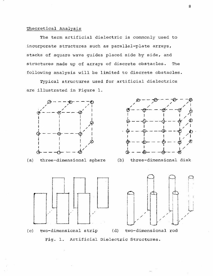
The term artificial dielectric is commonly used to

incorporate structures such as parallel-plate arrays,

stacks of square wave guides placed side by side, and

structures made up of arrays of discrete obstacles. The

following analysis will be limited to discrete obstacles.

Typical structures used for artificial dielectrics

are illustrated in Figure 1.

!Cr-- -e--- -0- - -(f) / / / /I

/ / / / ~- - -qr-- - -(lf - -qf ~ I 1 I I "'I I J. / &---4+-- -'-41-- .k <t> I I I T //I <r- -·-f-- --@-- --<? /b I I I I _, I t- - -tP- - - ~ - - t1S /®

~- -~--.--J---.Js/ (a) three-dimensional sphere (b) three-dimensional disk

1: u

/ / / / / /

/ / /

-~

(-o) two-dimensional strip (d) two-dimensional rod

Fig. 1. Artificial Dielectric Structures.

When .the electric f.ield is perpendicular to the rods in (d)

above, capacitive loading is produced, and E: is increased.

This method of increasing E: will be used in the design

criteria.

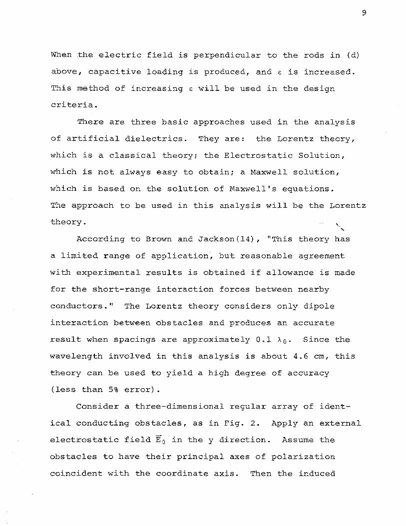
There are three basic approaches used in the analysis

of artificial dielectrics. They are: the Lorentz theory,

which is a classical theory; the Electrostatic Solution,

which is not always easy to obtain; a Maxwell solution,

which is based on the solution of Maxwell's equations.

9

The approach to be used in this analysis will be the Lorentz

theory.

According to Brown and Jackson(l4), "This theory has

a limited range of application, but reasonable agreement

with experimental results is obtained if allowance is made

for the short-range interaction forces between nearby

conductors." The Lorentz theory considers only dipole

interaction between obstacles and produces an accurate

result when spacings are approximately 0.1 AQ· Since the

wavelength involved in this analysis is about 4.6 em, this

theory can be used to yield a high degree of accuracy

(less than 5% error).

Consider a three-dimensional regular array of ident-

ical conducting obstacles, as in Fig. 2. Apply an external

electrostatic field Eo in the y direction. Assume the

obstacles to have their principal axes of polarization

coincident with the coordinate axis. Then the induced

dipole moment p of one obstacle is in the y direction for

an applied field in the y direction. y

z

/ /

G~-' I I ; I ;

d{--

·----~, -- -~~"'r / l " I / ~

--<r--t--EP I r l I I

- -t-- -C9-- J ---0 I //J I /'I l,/ I 1/' I

-4--t- -0 ;J'1 T ' I c I I I I /

a --..:::..... I' b " ........ , ~' .L I ~'

- - - -e--- :t -(!)"'

X

Fig. 2. Three-dimensional Artificial Dielectric.

10

If the dimensions of the obstacles are small compared

with their spacings, the field acting to polarize any one

obstacle may be assumed to be.a uniform field equal to the

field at the center of the obstacle. The polarizing field

at the obstacle located at the origin has only a y component

Eey because of symmetry. As stated before, the induced

dipole moment is proportional to the field E as follows; ey

p = a e: 0E • e ey (4)

For nonsymmetrical obstacles, a is different along differ­e

ent directions, and in general is a tensor quantity. The

number N of obstacles per unit volume is equal to (abc)- 1 ,

therefore, the dipole polarization per unit volume is

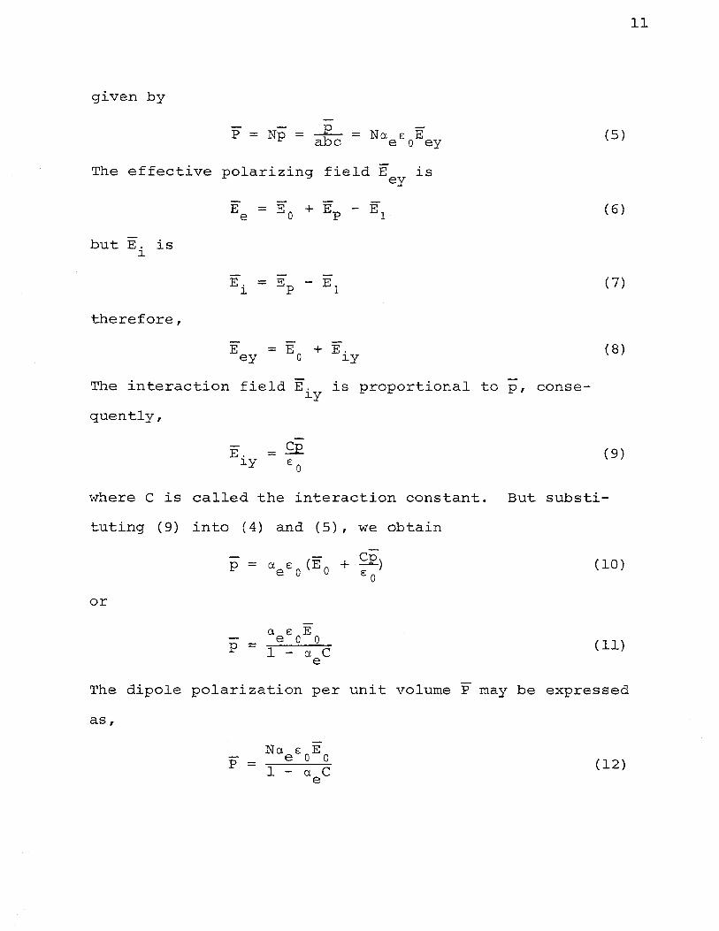
given by

= _.E__ab c = N a e: E e o ey P= Np

The effective polarizing field E is ey

but E. is 1.

therefore,

The interaction field E. is proportional to p, conse­l.Y

quently,

E. l.Y

( 5)

(6)

(7)

( 8)

(9)

where C is called the interaction constant. But substi-

tuting (9) into (4) and (5}, we obtain

P = aee:o (Eo + Cp) e:o

or

a e: E P = e o o

1 - (l c e

(10)

(11)

The dipole polarization per unit volume P may be expressed

as,

p = Na e: E e o o 1 - (l c

e (12)

11

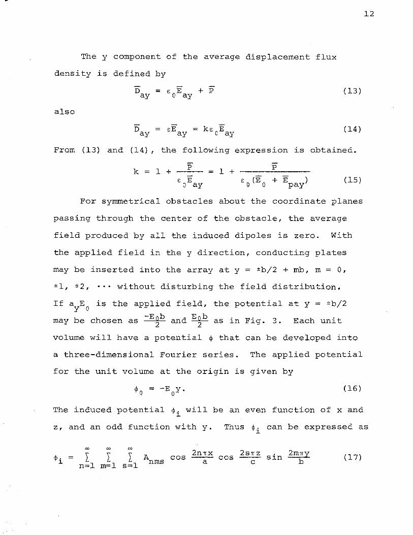
The y component of the average displacement flux

density is defined by

D =e:E +P ay o ay (13)

also

Day = e:Eay = ke:OEay (14)

From (13) and (14) 1 the following expression is obtained.

k = 1 + p = 1 +

p

e: E o ay (15)

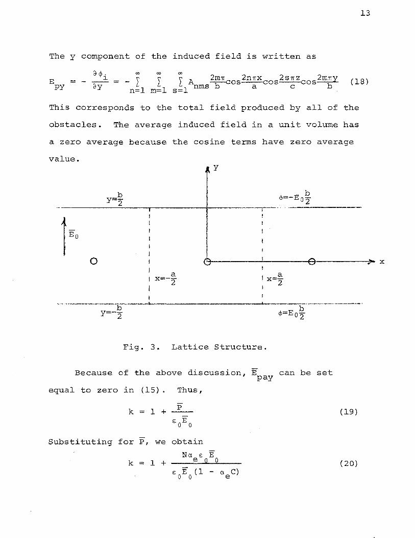
For symmetrical obstacles about the coordinate planes

passing through the center of the obstacle, the average

field produced by all the induced dipoles is zero. With

the applied field in the y direction, conducting plates

may be inserted into the array at y = ±b/2 + mb, m = 0,

±1, ±2, ···without disturbing the field distribution.

If a E is the applied field, the potential at y = ±b/2 y 0

may be chosen as -E~b and E~b as in Fig. 3. ~ach unit

volume will have a potential $ that can be developed into

a three-dimensional Fourier series. The applied potential

for the unit volume at the origin is given by

$ = -E y. 0 0

(16)

The induced potential $· will be an even function of x and ~

12

z, and an odd function with y. Thus ~i can be expressed as

00 00 00

cfl· = I I I Anms cos 2n7rx cos 2s7rz sin 2m7ry (17) ~ n=l m=l s=l a c b

13

The y component of the induced field is written as

E py

d ¢. ~

=- -- = ay (18)

This corresponds to the total field produced by all of the

obstacles~ The average induced field in a unit volume has

a zero average because the cosine terms have zero average

value.

0 a x=--2

y

(~----------~--------~+-----------~ X

Fig. 3. Lattice Structure.

Because of the above discussion, E can be set pay

equal to zero in ( 15) . Thus,

k 1 + p

= (19) e: OE 0

Su~stituting for P, we obtain

k = 1 + N.a e: E " ~ Q 0 (20)

e: E ( 1 - aeC) 0 0

14

which yields

k = Na e

1 + 1 - 0'. c e

( 21)

This expression is known as the Clausius-Massotti relation.

This expresses the dielectric constant k as a function of

the obstacle polarizability a , the interaction constant e

C, and the number of obstacles N. As stated in the intro-

duction, the obstacles are immersed in a low-dielectric

constant filler. Equation (21) is the dielectric constant

relative to the dielectric constant of the filler material.

The main reason for the preceding analysis is to show

that the dielectric constant varies with the number of

conducting obstacles N.

Experimental Design of Slug to be Placed in the Horn Antenna.

The design of the slug will be based on the fact that

the dielectric constant can be made to vary from the feed

end of the horn to the media. The techniques of designing

a variable dielectric constant slug (as a function of

distance) will make use of the expressions established in

the theoretical analysis.

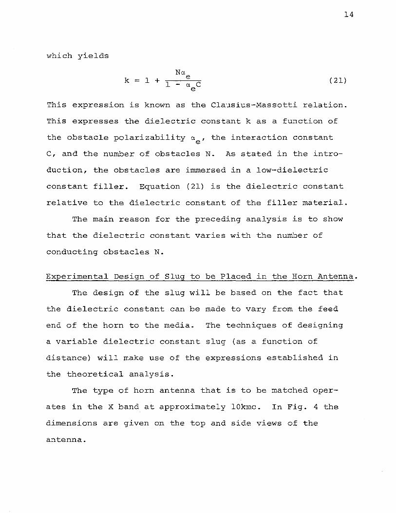
The type of horn antenna that is to be matched oper-

ates in the X band at approximately lOkmc. In Fig. 4 the

dimensions are given on the top and side views of the

antenna.

15

The dielectric constant of water is approximately 55

at 25°C. The dielectric constant of air is 1, therefore,

e: will have to be increased (in a manner which will be

discussed later) in order to match the antenna. As stated

previously, the obstacles will have to be perpendicular to

the electric fields, in order to increase e:. Also, for

the analysis in the previous section to coincide, the

obstacle {rods in this case) will have to be as in Fig. 5.

The oross~sectional view now coincides with that of Fig. 2.

3.5'

3.3"

t 1'

(a) top view

.5"

toE'------ 4 • ...1:::-"'11----;;.t

(b) side view

.9~

Fig. 4. Top and Side View of Horn Antenna

16

The size of the holes that are drilled in the slug will

have to be small compared with the spacings. The spacings

are limited to 0.1 A0 or about 0.46cm. This will necessi­

tate the use of small drill bits. In order for small holes

to be drilled, a material will have to be selected which is

tightly packed (nonporous) such as polystyrene. The mater-

ial chosen should have a dielectric constant close to one.

Styrofoam, which has a k of 1.03, was chosen by the author

and tested. The type of conducting obstacles used in the

drilled holes was water. The results will be discussed in

the conclusion.

I'-............. ,.....__ -

~~---------------------~ ~...,..... __ _

Fig. 5. Top View of Antenna. y

0 0

a 0 0

c Cl 0 0 0 0

0

drilled holes

.. X

X

Fig. 6. Cross-sectional View of Antenna.

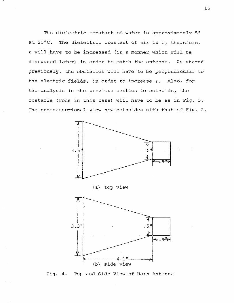
A method of increasing E by increasing the number of

obstacles will now be discussed. The cross-section of the

slug should be divided into a number of equal sections as

in Fig. 7.

l l

9 I 8 I 7 I I I I

~

I I I --...---..

1 I l I 6j5!4~312tl

\ I I I I I

..1··· • ~ _J. ................... :.-...............

1_ .. ..-t--·

Fig. 7. Cross-section

Next a distribution (straight-line, logarithmic, etc.)

should be chosen which describes the variation of e in the

range 1 .::_ £ < 55 with distance. A sample of the material

used for the slug should be prepared in order that it may

17

be placed in the waveguide and its properties determined.

The sample should consist of a 1" x ~~~ x 1 11 block of mater­

ial with holes drilled in it. This size was chosen because

of the dimensions of the waveguide. Whatever conducting

material is chosen the obstacle will be in the holes. The

dielectric constant is found £or.each different hole distri-

bution. A graph is plotted of the dielectric constant £

versus the number of holes as in Fig. 8. Given the £

needed in the chosen distribution, the number of holes that

hap to be drilled per unit volume can be found from this

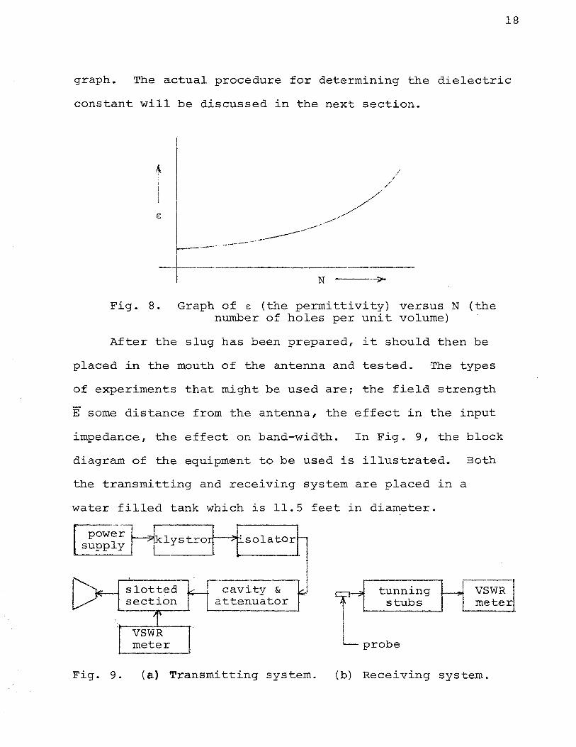
18

graph. The actual procedure for determining the dielectric

constant will be discussed in the next section.

e:

N • >

Fig. 8. Graph of e: (the permittivity) versus N {the number of holes per unit volume)

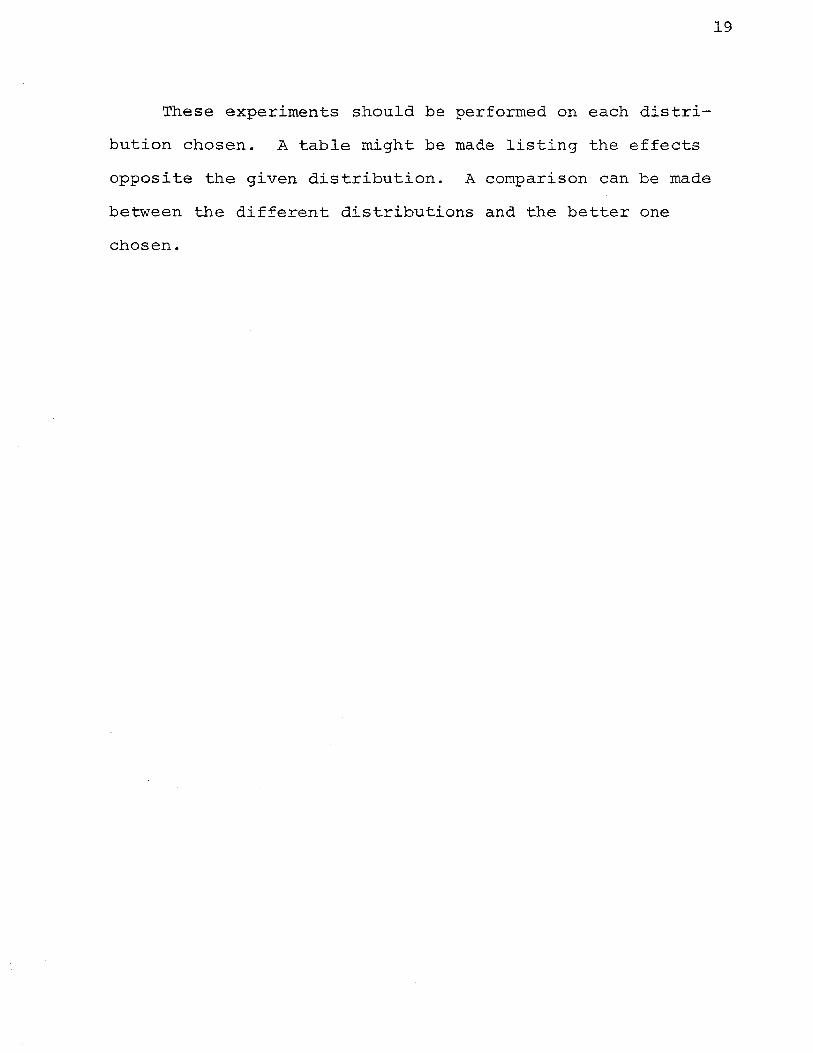
After the slug has been prepared, it should then be

placed in the mouth of the antenna and tested. The types

of experiments that might be used are; the field strength

E some distance from the antenna, the effect in the input

impedance, the effect on band-width. In Fig. 9, the block

diagram of the equipment to be used is illustrated. Both

the transmitting and receiving system are placed in a

water filled tank which is 11.5 feet in diameter.

'•

slotted section

I!J--v-----sw~R----r

meter

cavity & attenuator

tunning t-.,~7

~ stubs

.___ probe

~ VSWR meter

Fig. 9. (a) Transmitting system. (b) Receiving system.

These experiments should be performed on each distri­

bution chosen. A table might be made listing the effects

opposite the given distribution. A comparison can be made

between the different distributions and the better one

chosen.

19

20

IV. DISCUSSION OF THE MEASUREMENT OF DIELECTRIC PROPERTIES

Introduction

In the laboratory, electromagnetic waves are confined

by various types of boundaries. This might be looked upon

as a disadvantage, but the reflection and refraction of

fields by conductors or dielectrics provide the means for

quiding and alternating the fields and for measuring the

dielectric properties of media.

Theoretical Analysis

The incident, reflected, and refracted waves are

"tied together" by the boundary condition which states

that the tangential component of E and H must be continuous

in traveling from one media to another. The amplitudes as

well as the phases must be continuous. The first condition

(amplitudes are continuous) leads to Fresnel's equation.

The second condition (phases being continuous) introduces

Snell's laws of reflection and refraction. Snell's laws

and Fresnel's equations together determine the intensity,

direction, and polarization of the reflected and refracted

waves as a function of the properties of the two adjoining

media.

When dealing with reflection and refraction character­

istics, the relative amplitude and intensities of the waves

are of importance, not the absolute values.

21

The ratio of the reflected amplitude to the incident

amplitude at the boundary is defined as the reflection

coefficient r.

r ~ Er E ' Eo

( 22)

The subscript 1 indicates the reflected wave and the sub-

script 0 indicates the indicent wave. By defining the

ratio of the amplitudes of the transmitted to the incident

as the transmission coefficient t, we have

( 23)

The subscript 2 indicates the transmitted wave. After

es'tablishing the above relationships, one of Fresnel's

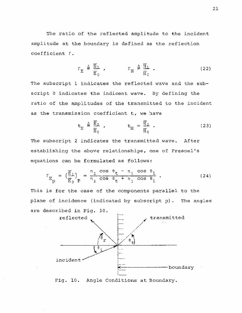
equations can be formulated as follows:

= (~) Eo P

n2 cos et - n1 cos ai -

n 2 cos et + n 1 cos ei ( 24)

This is for the case of the components parallel to the

plane of incidence (indicated by subscript p}. The angles

are described in Fig. 10.

reflected transmitted

incident

IE'-----------boundary

Fig. 10. Angle Conditions at Boundary.

In the above equation, n 1 and n 2 are the intrinsic imped­

ances of media 1 and 2.

22

The angle of incidence ei and the angle of refraction

(or transmission) et are interrelated by Snell's refraction

law: y2 . sin e. =-- s~n et

~ 'Y]. ( 25)

where y 1 and y 2 are the propagation constants of media 1

and 2 respectively, or in another form

s~n et = *~ s~n e. v~

~ 2 2

In order to simplify Fresnel's equation, perpendicular

( 26)

incidence is assumed (ei = et = 0), therefore Fresnel's

equation becomes

( 2 7)

The incident and reflected waves superpose and form

by interference a standing-wave pattern. This resulting

standing-wave pattern will help in determining the dielec-

tric properties of the media.

Let Ey and Hz propagate in the positive x direction

through medium 1 and strike the boundary of medium 2 at

x = 0 as shown in Fig. 11. The reflected wave returning

in the negative x direction combines with the forward

wave to yield the resulting standing wave. The E and H

fields of the standing wave pattern are expressed as follows:

23

E = E e ( j wt-y 1 x) + E (jwt+y 1x) y1 0 1e

( 28)

H = H ( jwt-y 1 x) + H e (j wt+y 1 x) z1 oe 1

Now l@t r 0 and -r 0 be the reflection coefficients of the

electric and magnetic waves at the boundary x = 0. Express-

ing the resulting fields we have

E = Eoe (jwt-yl x) + r E (jwt+ylx) yl o oe

(29)

H = H (jwt-y 1x) - r H (jwt+ylx) zl oe o o e

E = Eoejwt[e-ylx + r 0e Y 1 xl yl

H Eo jwt[ -y 1x r 0 e Y 1 x] = e e -

zl nl

(30)

z

Fig. 11. Formation of Standing Waves.

X

24

Assume, for the present, that the wave in media 2 continues

without further interference. Thus,

(31)

The reflection r 0 for normal incidence is given by

n - n 2 1 r -o - n2 + nl ( 32)

It can be seen from the above equation that if the

intrinsic impedances of the two media are equal, there

will be no reflection. Therefore,

nl = n2

anq, ( 33)

e:* 1

e:* 2

e:* 1 ll!

ll* = or e:* = ll* ll* 1 2 2 2

where * indicates a complex quantity. This condition re-

quires that both the electric and magnetic flux densities

must change by the same amounts in traveling across the

boundary between the two media.

The opposite extreme, total reflection, requires that

one intrinsic impedance must be much higher than the other

impedance. This can be accomplished by using a metal for

Gne of the media. The intrinsic impedance of a metal

(magneti9 loss n~glected} may be written as

jwll~ where jw /c:*)..l* n2 = m= y2 = * y2 2 2 2

~ but c:" cr2

n2 = = ffii = u 2 w I

2

n2 = ~ 2.

Because of the high conductivity a 2 , n 2 << n 1, the

reflection coefficient at the metal boundary becomes

ro = :::: -1

Now assume that media 1 is loss-free. Then

Under the above conditions Eqs. (29} become

E '2E jwt sin 21fX = -J e yl 0 A1

H 2E 0 ejwt 27TX

= cos zl nl A1

2j

j27TX + j-21fX e -- e A A 1 1

2

25

( 3 4)

( 35)

( 3 6)

( 38)

(39)

Now by changing over to the real field components we obtain

R (II ) 2E 0 sin wt sin 27TX - Al e . YI

2E 0 (40)

R (H ) wt 21fX = cos cos

A.l e z 1 n1

These equations represent a standing wave for which

the electric field has its nodes at the metal boundary and

at a distance which is given by

21rX sin = 0 A.l

= n1T nA.l

X = -2- ( 41)

In this case, x is the distance from the metal surface as

shown in Fig. 13.

The antinodes of E are located at the following

points:

sin 27rX ffi1T (2k 1) = 2 m = -A.l

mA.l ( 4 2)

where X = -4- k = 1, 2, 3, 4, ...

Again x is the distance explained above. The nodes and

antinodes for the magnetic field are in reverse order.

The ratio of a component of E to a component of H is

called the wave impedance in the direction defined by the

26

cross-product rule as applied to the two components. Thus,

continu~ty of tangential E and H requires that wave imped-

ances normal to a material boundary must be continuous.

Using the symbol Z to represent the wave impedance in the X

x direction, we have

The ratio of the two fields at the boundary (x = 0) , is

given by

( 43)

( 44)

The wave impedance (Zx(O)) can be found by measuring

the amplitude jr 0 ! and the phase angle 2~ of the reflec­

tion coefficient r 0 •

27

By measuring the distance x 0 of the first minimum from

the boundary of the dielectric(l2), the phase angle is

given by

( 45)

The ratio of the electric to the magnetic field strength

at this minimum is expressed as

= nl

1- lro je-2a.lxo

1 + lr 0 je-2 a.1xo

Since media 1 was assumed loss-free, (a. 1 ::::: 0) equation

(46) reduces to

E 1 + I r 1· MAX o EMIN . = l - I r o I

(46)

( 4 7)

This ratio is called the voltage standing-wave ratio (VSWR) •

By measuring the VSWR and the distance to the first

minimum (x 0 ), the magnitude and phase of the reflection

coefficient may be determined. After the reflection

coefficient is known, the wave impedance Z (0) is found X

providing the intrinsic impedance n1 is known.

From the previous discussion on wave impedances, it

is clear that the wave impedance for normal incidence is

the same whether traveling toward the boundary or away

from the boundary. Thus,

z ( 0) X

=

E {0) yl

H (0) zl

=

E ( 0) Yz

( 48)

If no further reflection takes place in medium 2, the wave

impedance measured by the VSWR in medium 1 is directly

equal to the intrinsic impedance of medium 2. Therefore,

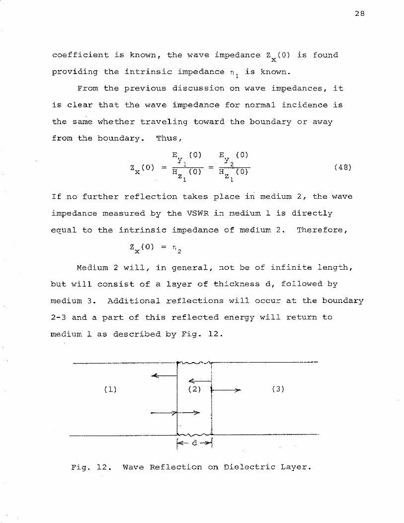
Medium 2 will, in general, not be of infinite length,

but will consist of a layer of thickness d, followed by

28

medium 3. Additional reflections will occur at the boundary

2-3 and a part of this reflected energy will return to

medium 1 as described by Fig. 12.

'* -(1) (2) .... ( 3) , '

, ,

-

......

Fig. 12. Wave Reflection on Dielectric Layer.

29

This complex situation will not effect the measurement

of the standing-wave pattern in medium 1, but will change

the requirements for the reflection coefficient r 0 and the

wave impedance Z (0) • Before going on with this discussion, X

the wave impedance Z (0) will be reformulated in terms of X

the directly measurable quantities, inverse VSWR, x 0 , and

A 1 , in order to arrive at a usable expression for actual

expression for actual calculations. Let

ro -2u = e

where u = p + • tp J

then the wave impedance is given

1 + r Zx(O) 0 = Tll 1 - r

0

-u u zx (0}

e (e = Tll -u u e (e

u + -u e e

zx (0} 2 = Tll = Tli u -u e - e 2

and the inverse VSWR becomes

by

1 + -2u e = Tll -2u 1 - e

( 4 9)

-u + e ) -u - e }

(50}

cosh u = n 1 coth u (51) sinh u

EMIN

EMAX =

1 -2p - e = tanh p (52)

By expanding coth u and using the relation for tp and

x 0 , the wave intpedance can be expressed (This development

may be found in the Appendix.) in terms of measurable

quantities.

30

Z(O) = n1 tanh E - j cot 1jJ

1 - j tanh p cot 1jJ

EMIN 2rrx 0 (53)

- j tan EMAX A.l

1 j EMIN 2rrx 0

- tan EMAX A.l

Z(O) = n 1

The wave impedance Z (0) is now determined experiment­x

ally by measurements of the VSWR pattern in medium 1.

In order to obtain from the previous equation the

properties of medium 2, the situation at the boundary 2-3

at x = d has to be considered.

Due to the reflection at the boundary 2-3, there will

be a standing wave set up in medium 2. The fields are

given by

E y2

= E jwt[ -y (x-d) + r y 2 (x-d)] 2 e e 2 2 3e

(54)

The wave impedance in the negative x direction at x = 0

Z (0) is expressed as -x

z ( 0) = -x

r e-y2d 2 3

r e-y2d 2 3

(55)

If the transmitted wave continues in medium without inter-

ference, th~n the r~flection coefficient at boundary 2-3

bec:ome·s

r23 = (56)

Now, if the medium 3 is metal, total reflection will occur

at X = d. ThUS,

Substituting the above result into Eq. (55), the wave

impedance Z (0) becomes -x

z ( 0) -x e y2d - e -yzd

= n2 ey2d + e-y2d

This will be called the "short-circuit measurement" of

medium 2.

(57)

This one measurement will not suffice for all media,

therefore, another measurement must be performed. In this

case, the shorting metal plate will be placed a distance

~ behind d as shown in Fig. 13.

(1) (3)

/ L.

~- d +"----- ~ -~ x=O

Fig. 13. Arrangement for Measuring a Dielectric 2.

Due to the reflection at boundary 2-3, a standing wave

patt~rn will be formed in medium 3. These fields are

expressed as

31

(58)

= jwt[ -y3(x-d-6) y 3 (x-d-6)] e e ~ e

As stated before, the wave impedance at x = d is the same

in either direction (-x or +x}. Thus,

zx (d) = z (d) -x (59)

E E y2 ~ = H H

( 60} z2 z3

1 + r 2 3 e Y 3!::. -y3h. e n2 = n3 1 - r23 e Y 3!::. -y36 + e

1 + r23 n3 eY36 -y3h.. e = -1 - r23 n2 y 36 -y36. e + e ( 61)

n3(1- e-2y3h.) - n2(1 + e-2y36.)

n3(1- e-2y3!::.) + n2(1 + e-2y3!::.)

A.3 Now if h. is made equal to~ (quarter wave length),

this measurement will be called an "open-circuit measure-

t '' th d . 3 . 1 f ( .. 2 1T) men • Assume at me 1um 1s ass- ree y 3 =-Jr-. 3

From the above equation, r 23 then becomes equal to 1.

The wave impedance Z (0} becomes X

z ( 0) = n 2 coth y 2 d ( 6 2)

32

The ratio of input impedance at x = 0 to the intrinsic

impedance is given in Eq. (53). Thus,.

EMIN j tan

21fXO

z ( 0) EMAX A.l (63) = nl EMIN 2rrx 0

1 - j EMAX

tan A.l

When medium 2 is terminated in a shorting plate (~ = 0)

the impedance becomes

( 6 4)

Dividing by n 1 and transposing gives

( 65)

The relationship between·the intrinsic impedance and the

propagation factor is

n =

Now (66)

=

Substituting this into Eq. (65) and dividing by d gives

= z ( 0)

yldnl

If medium 1 is loss-free {y = j 2 'TT), this reduces to 1 1.. 1

= -jA.

1 2rrd

( 6 7)

( 6 8)

When A is equal to a quarter wavelength of medium 3, the

open-circuit condition results. Therefore,

Z ( 0) = n coth y d ( 6 9) 2 2

33

' and again for a loss-free medium 1, we have

= -j A

1 21Td

Z(O) n1

( 7 0)

Equations (68) and (70) are expressions relating the

unknown y to the measured quantities d, A1 , EMIN/EMAX'

and x 0 • Equation (68) is for the sample mounted in front

of a shorting plate and equation (70) is for the sample

a quarter wavelength away. One stipulation on these

expressions is that the bounding conductor walls are uni-

form throughout the three media. Equations (68) and (70)

may be rewritten as follows:

=

=

-j A 1

2'JTd

-jA 1

2'JTd

E MIN . t - J an

EMAX

21TX 0

EMIN Z'ITXO l - j tan

EMAX Al

These equations may be expressed in polar form:

tanh TejL J·r = Ce .,.

= Cejz;;

( 71)

( 72)

A survey map has been drawn by S. ROO:>erts ( 10) using the

argument L as the ordinate, and the absolute value of T as

34

the abscissa, where C and ~ are parameters of intersecting

curves; and T and ~ are expressed in degrees. Detailed

charts may be found in work by von Hippel(l2).

The relationship between e~ and y 2 depends on the

cut-off wavelength A of the wave guide. The cut-off c

35

wavelength A is the lowest free-space wavelength for which c

propagation in a particular mode is possible. For the

rectangular wave guide (TE 01 m~e), the cut-off wavelength

Ac is two times the width.

For TE modes in rectangular wave guides, the separation

equation can be expressed as

where

( 7 3)

where k = -jy z z

[em;) 2 + (n~) 2~

(7 4)

Yl = j~w2ll£- [(m~)2 + (n~)2]

For propagation, the radical must be positive. Therefore:

w2ll e: > (~) 2 + (!!.!) 2 - a b ( 7 5)

(!!!.:!!..) 2 + (n7T)2. a b

w > c - 'j.IE:

(~) 2 + (!!.,._) 2 f 2a 2b

> c - 'j.IE:

1 ( 7 6)

"c v l'j.le: 1 = r = =

1(~) 2 c (!!!.-) 2 + '{£.._,) 2 + (!!..__) 2 2a 2b 2a 2b

'j.IE

The propagation constant can be written for region (2) as

follows:

k2 = k2 + {27T) 2 2 z2 A. c

k2 = k2 - (27T)2 zl 1 "c

But, from previous paragraphs, we recall that

From the above equations, we obtain

e:* = 2

Multiplying by e: 0 gives

2 w 11 0 e: 0

( 77)

( 78)

( 79)

36

From previous work, we have

y (2.) 2

2'1T

Now by making a substitution we obtain

e::* = e: 2 0

37

( 80)

(81)

(82)

From.the above equation, the complex permittivity e::; can be

found from the measureable quantities A1 , Ac' d and the

calculated quantity y 2 d.

Procedure for Measuring the Dielectric Properties

The laboratory equipment available determines the

procedure and method that should be used. A type of wave-

guide instrument has been developed for dielectric

38

measurements. A stabilized reflex klystron oscillator

radiates monochromatic waves of a eertain frequency into a

hollow, rectangular wave guide; they are reflected by a

shorting metallic boundary at the other end. Standing waves

' are set up and can be measured by a traveling probe detect-

or along a narrow slot in the top of the guide parallel to

its axis. The dielectric sample is placed in the closed

end of the guide opposite the ·r ransmi tter. For the open

circuit measurement; the sample is located a quarter wave-

length ahead of the short; for the short~circuit measurement,

the sample is placed in direct contact with the short. The

sample should fit as closely as possible to the short and

walls of the guide, and its faces should be perpendicular

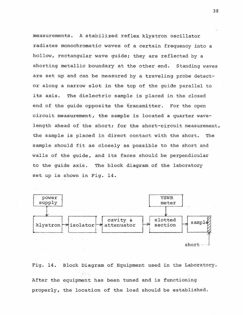
to the guide axis. The block diagram of the laboratory

set up is shown in Fig. 14.

----------, cavity &

attenuator

[ VSWR J meter -- . . .

slotted section sampl

short -- ·- -- -

Fig. 14. Block Diagram of Equipment used in the Laboratory.

After the equipm~nt has been tuned and is functioning

properly, the location of the load should be established.

39

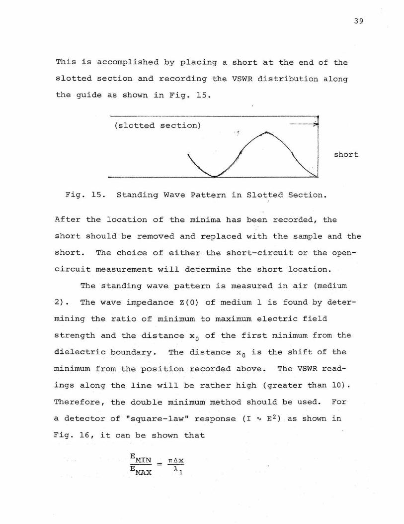
This is accomplished by placing a short at the end of the

slotted section and recording the VSWR distribution along

the guide as shown in Fig. 15.

(slotted section) ________ ;J.

. <

short

Fig. 15. Standing Wave Pattern in Slotted Section.

After the location of the minima has been recorded, the

short should be removed and replaced with the sample and the

short. The choice of either the short-circuit or the open-

circuit measurement will determine the short location.

The standing wave pattern is measured in air (medium

2). The wave impedance Z(O} of medium 1 is found by deter-

mining the ratio of minimum to maximum electric field

strength and the distance x 0 of the first minimum from the

dielectric boundary. The distance x 0 is the shift of the

minimum from the position recorded above. The VSWR read-

ings along the line will be rather high (greater than 10) .

Therefore, the double minimum method should be used. For

a detector of "square-law" response (I rv E 2 ) . as shown in

Fig. 16, it can be shown that

EMIN

EMAX

40

A.l The half wavelength ~ in the air space of the guide may be

obtained by measuring the distance between two minima of

the standing wave pattern. The measurable quantities

EMIN/EMAX' x 0 , d, and A. 1 can be determined from this

procedure.

I I

T --- 1MIN

----~--------~~--------~--------------~ X

Fig. 16. Square Law Measurements.

Summarizing, the procedure of determining £~ begins

with measurements of EMIN/EMAX' x 0 , d and ;,. 1 • From these

measured values, C and s are calculated from Eq. (71).

From C and s the values of T and ' are found by using the

specified charts. By dividing Tej' by d, y 2 is obtained.

Finally £ ~ is determined from y 2 by Eq. (81) or Eq. (85).

For nonmagnetic materials, just one of the two measure-

ment methods (short-circuit or open-circuit) has to be

performed. Magnetic materials require a separate calcula-

tion for Z2 (0) and y 2 because the impedance is of ratio

form and the propa<J~tion factor is of product form, both

forms involving lJ~ and s~. In this case both measurement

methods have to be performed.

41

V. CONCLUSIONS

The main problem in this matching technique is the

selection of the material for the slug and also that of the

conducting obstacles.

The material for the slug must be a nonporous, light­

weight dielectric with a dielectric constant close to one.

The only restriction placed on the obstacle, aside from

being small, is that it have low losses. There is a wide

variety of these materials from which to choose.

In the author's actual experiments on styrofoam

dielectric, difficulties came up because of the choice of

materials and obstacles. Styrofoam was chosen because of

its light weight and low dielectric constant (1. 03). The

only problem with this material is that it is too porous.

After the holes were drilled and water placed in these

holes, the sample was then placed in the waveguide equip­

ment. Before all of the measurements needed could be taken,

most of the water either had leaked out of the sample or

was absorbed by the styrofoam. From this problem, irratic

data resulted. The problem may be bypassed by the use of

a different obstacle (a solid material). If water is to

be used as the obstacle, a different material should be

used for the slug. Polystyrene is a non-porous, light­

weight material with a dielectric constant of 2.56. Some

compromise will have to be made with the materials to get

the best results.

The method of determining the dielectric properties

discussed in the thesis gave reasonably accurate results

of solid samples tested. The value of the dielectric

constant of styrofoam was found to be 1.035 which compares

favorably with that given by von Hippe!.

The author feels that a suitable matching slug can

be designed using the procedure discussed under artificial

dielectrics to match an antenna such as a horn to a dense

media such as water. The dielectric properties of this

matching slug may be determined by the proper use of the

techniques discussed under the measurement of dielectric

properties section.

42

43

APPENDIX

Wave Impedance Expressed in Te~ of Measurable Quantities.

Starting with the wave impedance,

Z(O) = n 1 coth u

Make the substitution,

u :::: p + jljl

where

and expand coth u.

z ( 0) cosh (E + = nl sinh (p +

Z(O) cosh p cos = nl sinh p cos

Divide (A-4) by sinh p.

z (0) coth E cos = nl cos l/1 + j

Divide (A-5) by sin t/J

z ( 0) coth E cot = n I cot lJ! + j

cot 1/J + j

j $) j ,P}

$ + $ +

$ + coth

$ + coth

tanh

z ( 0) = nl tanh E

tanh E cot t/J + tanh p

z (0) cot 1/J + . tanh = nl " . J j + tanh p cot

Multiply (A-8) by ( -j) .

tanh E - j cot =

j j

j p

j. p

E

j

E t/J

1jJ z (0) nl 1 - j tanh p cot

sinh cosh

sin sin

t/J

(A-1)

(A-2)

(A-3)

p sin 1/J p sin $

(A-4)

~ lj1

(A-5)

(A-6)

(A-7)

(A-8)

(A-9)

44

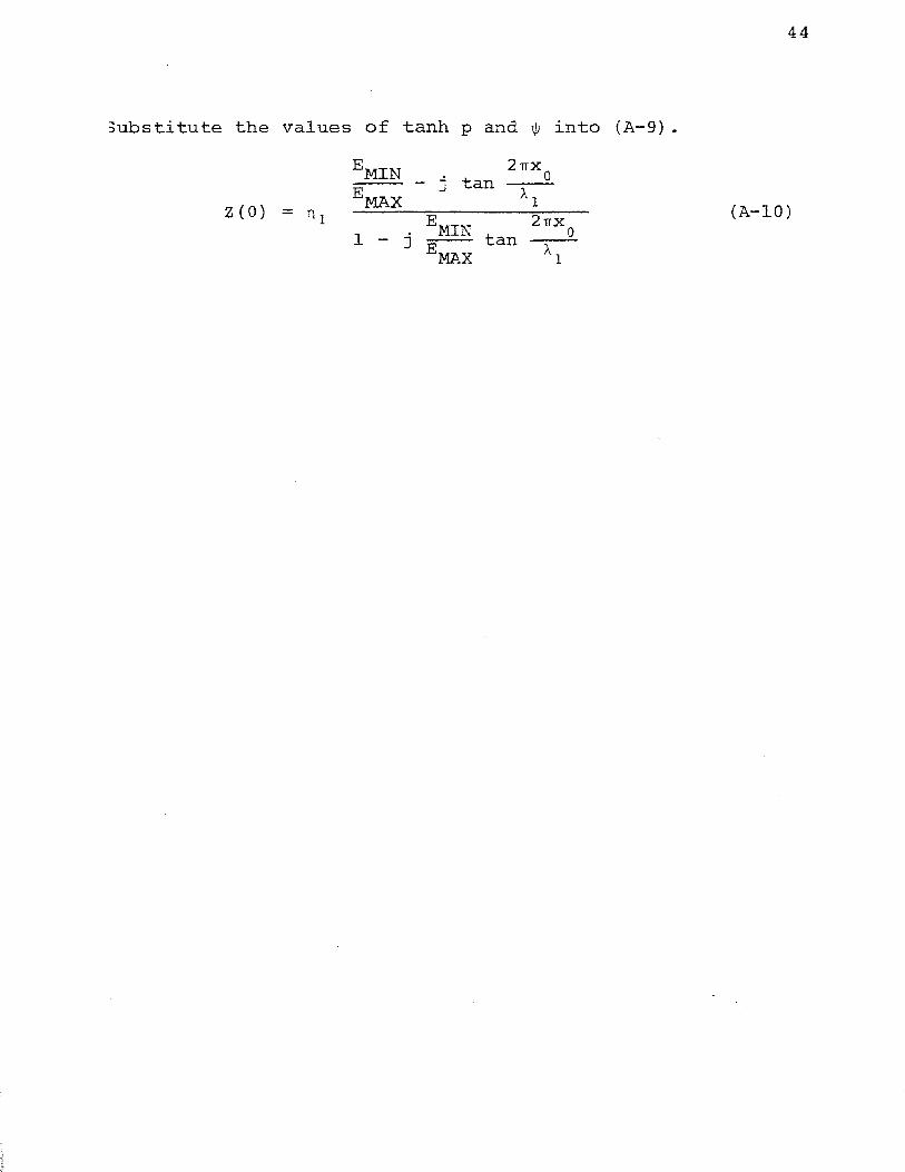
:iubstitute the values of tanh p and I)J into (A-9).

Z{O) = n 1 EMIN

1 - j tan EMAX

(A-10)

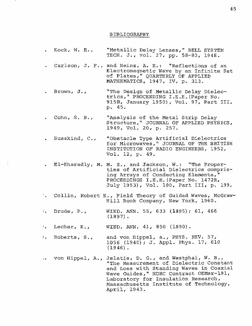
BIBLIOGRAPHY

Kock, W. E., "Metallic Delay Lenses," BELL SYSTEM TECH. J., vol. 27, pp. 58-83, 1948.

45

Carlson, J. F., and Heins, A. E.: "Reflections of an Electromagnetic Wave by an Infinite Set of Plates," QUARTERLY OF APPLIED MATHEMATIGS, 1947, IV, p. 313.

Brown, J., "~he Design of Metallic Delay Dielec­trics 1 " PROCEEDING I • E. E. (Paper No. 915R, January 1950), Vol. 97, Part III, p. 45.

Cohn, S. B., 11Analysis of the Metal Strip Delay Structure," JOURNAL OF APPLIED PHYSICS, 1949, Vol. 20, p. 257.

Susskind, C., "Obstacle Type Artificial Dielectrics for Microwaves, " JOURNAL OF THE BRITISH INSTITUTION OF RADIO ENGINEERS, 1952, Vol. 12, p. 49.

El-Kharadly 1 M. M. Z., and Jackson, W.: "The Proper­ties of Artificial Dielectrics compris­ing Arrays of Conducting Elements," PROCEEDINGS I.E.E. (Paper No. 1472R, July 1953), Vol. 100, Part III, p. 199.

Collin, Robert E., Field Theory of Guided Waves, McGraw­Hill Book Company, New York, 1960.

: . Drude , P. ,

1. Lecher, E. ,

1 • Roberts , S . ,

WIED. ANN. 55, 633 (1895); 61, 466 (1897).

WIED. ANN. 41, 850 (1890).

and von Hippel, a., PHYS. REV. 57, 1056 (1940); J. Appl. Phys. 17, 610 (1946) .

von Rippel, A., Jelatis, D. G., and Westphal, W. B., "The Measurement of Dielectric Constant and Loss with Standing Waves in Coaxial Wave Guides," NDRC Contract OEMsr-191, Laboratory for Insulation Research, Massachusetts Institute of Technology, April, 1943.

von Hippel, A., DIELECTRIC MATERIALS AND APPLICATIONS, Technology Press of M. I. T. and John Wiley and Sons, New York, 1954, Sec. II a, 2.

von Hippel, A., DIELECTRICS AND WAVES, John Wiley and Sons, New York, 1954.

Brown, J. and · ..

Jackson, W., "The Properties of Arti­ficial Die~ectrics at Centimetre Wavelengths, 11 PROCEEDINGS I.E .E. (Paper No. 1699i., January 1955), Vol. 102 Part B, pp. 11-16.

46

VITA

Paul Arthur Ray was born on December 21, 1941, in

'lla, Missouri. He received his primary and secondary

lucation in the Rolla Public Schools.

In 1959 he enrolled in the Missouri School of Mines

1d Metallurgy. He completed his course work for his

tchelor of Science degree in Electrical Engineering in

1ly 1963, and enrolled in the graduate school.

He was married to Patricia Strothkamp in August 1963.

While in school, he was a member of Blue Key, Theta

tu, Interfraternity Council, Student Union Board and

)uncil, Sigma Tau Gamma, and '!'he Institute of Electrical

1d Electronics Engineers.

47