shear strength and displacement …prltap.org/eng/wp-content/uploads/2017/10/carlos-adorno.pdfshear...

SHEAR STRENGTH AND DISPLACEMENT CAPACITY

OF SQUAT REINFORCED CONCRETE SHEAR WALLS

by

Carlos M. Adorno-Bonilla

Dissertation submitted in partial fulfillment

of the requirements for the degree of

DOCTOR OF PHILOSOPHY

in

CIVIL ENGINEERING

UNIVERSITY OF PUERTO RICO

MAYAGÜEZ CAMPUS

2016

Approved by:

________________________________

Daniel A. Wendichansky-Bard, Ph.D.

Member, Graduate Committee

__________________

Date

________________________________

Luis A. Montejo-Valencia, Ph.D.


__________________

Date

________________________________

Ricardo R. López-Rodríguez, Ph.D.


__________________

Date

________________________________

Aidcer L. Vidot-Vega, Ph.D.

President, Graduate Committee

__________________

Date

________________________________

Ismael Pagán-Trinidad, M.S.C.E.

Chairperson of the Department

__________________

Date

________________________________

Elsie I. Parés-Matos, Ph.D.

Representative of Graduate School

__________________

Date

ii

ABSTRACT

Squat reinforced concrete (RC) walls are essential structural components in nuclear power

facilities (NPP) and in many civil structures. An adequate prediction of the shear strength and

displacement capacity of these elements are important for the seismic design and performance

assessment of structures whose primary lateral force resisting system is comprised by squat

walls. These walls have aspect ratios less than or equal to 2. Due to their geometry, squat shear

walls tend to have shear-dominated behavior while exhibiting strong coupling between flexural

and shear responses. This dissertation presents an evaluation of current expressions for the

prediction of peak shear strength and displacement capacity of squat RC walls available in US

design codes and in the literature. An updated database was assembled with the results of

moderate to large-scale experimental tests walls with shear-dominated failures and subjected to

cyclic loads found in the literature. Key parameters influencing the peak shear strength and

displacement capacity were identified and improved predictive equations were developed by

calibration against the available data. Multiple-linear regression analyses were used to develop

the predictive equations. It was found that the peak shear strength of such walls has not been

adequately addressed by current US code equations in ASCE 43-05 and ACI 349-13 / ACI 318-

14 since there is significant scatter on the predictions. It was also found that the peak shear

strength equations in current US codes and standards tend to over-estimate the strength of squat

RC walls with rectangular cross section, as well as to considerably under-estimate the peak shear

strength of the squat RC walls with enlarged boundary elements considered in the assembled

database. Experimental data suggested that allowable drift limits requred by ASCE 7-10 design

code provisions for damage control are unconservative for the case of squat walls. Finally, two

simplified analytical modeling approaches were presented. A Fiber-Based Model with flexure-

shear interaction and a Macro-Hysteretic model were studied. A tri-linear backbone, calculated

with the developed strength and displacement capacity expressions, was proposed to use in

conjunction with the Macro-Hysteretic model for the nonlinear-cyclic analysis of squat RC

walls.

iii

RESUMEN

Los muros robustos de hormigón armado son componentes estructurales esenciales en plantas de

energía nuclear y en muchas otras estructuras civiles. Una predicción adecuada de su resistencia

a cortante y capacidad de desplazamiento es importante para el diseño y evaluación de

desempeño de estructuras cuyo sistema de resistencia a carga lateral consiste de muros robustos.

Estos muros tienen una relación de aspecto igual o menor a 2. Debido a su geometría, los muros

de corte robustos tienden a mostrar un comportamiento dominado por cortante y un fuerte

acoplamiento entre las respuestas a flexión y a cortante. Esta disertación presenta una evaluación

de algunas expresiones existentes para la predicción de la capacidad a cortante y la capacidad de

desplazamiento, encontradas en los reglamentos de diseño de EEUU y en la literatura. Se

ensambló una base de datos actualizada, con los resultados experimentales de muros robustos de

escala moderada a grande, con falla dominada por cortante y sujetos a carga lateral cíclica,

hallados en la literatura. Se identificaron los parámeteros influyentes en la resistencia a cortante

y en la capacidad de desplazamiento, y se desarrollaron ecuaciones para la predicción de ambos,

mediante la calibración con los datos experimentales disponibles. Se usó el análisis de regresión

lineal multi-variable para el desarrollo de las ecuaciones. Se encontró que en los tres reglamentos

de construcción de EEUU, ASCE 43-05, ACI 349-13 y ACI 318-14, no se estima

adecuadamente la resistencia a cortante de los muros robustos de hormigón armado ya que estos

producen gran dispersión en los estimados de capacidad. Además se encontró que las provisiones

de los reglamentos de diseño de EEUU tienden a sobre-estimar la resistencia de muros robustos

con sección rectangular y a sub-estimar considerablemente la resistencia de muros robustos con

elementos de borde agrandados. El código ASCE 7-10 recomienda límites de distorción de

entrepiso permisibles que resultan no-conservadores para el caso de los muros robustos de

hormigón armado. Finalmente, se evaluaron dos metodologías existentes para la modelación de

muros robustos: un modelo basado en fibras con interacción flexión-cortante y un modelo

Macro-Histerético. Se propuso una curva tri-linear para estimar la envolvente de carga-

desplazamiento, calculada con las ecuaciones desarrolladas para la predicción de resistencia

máxima a cortante y la capacidad de desplazamiento. Se propuso utilizar el modelo de

envolvente tri-lineal en conjunto con el modelo Macro-Histerético estudiado para el análisis

cíclico no-lineal de muros robustos de hormigón armado.

iv

© Carlos M. Adorno-Bonilla 2016

v

This dissertation is dedicated to my parents, Eng. Ángel M. Adorno-Castro and Mrs. Carmen L.

Bonilla-Maldonado, for their patience and unconditional support during my academic career.

vi

ACKNOWLEDGEMENTS

I would like to thank my research advisor, Dr. Aidcer L. Vidot, for her continuous guidance and

support throughout the course of this research work. Her patience, dedication, willingness to

discuss ideas and findings, and disposition to clarify doubts during the whole research work has

been key for the completion of this dissertation.

I would also like to thank Professor Ismael Pagán-Trinidad, and Dr. Luis A. Montejo for their

availability to review this manuscript.

The help and technical support of Dr. Luis A. Montejo and Dr. Aidcer L. Vidot on the use of the

OpenSees analysis platform is greatly valued.

I would like to express my gratitude to Dr. Daniel A. Wendichansky and Dr. Ricardo R. López

for their review and insightful comments on this manuscript. Also, their encouragement and

helpful advices provided during my graduate student career is gratefully appreciated.

Special thanks are given to my family for their trust and unconditional support during every step

of my academic career, which has always allowed me to pursue my goals.

This research work was supported by awards NRC-HQ-12-G-38-0018 and NRC-HQ-84-14-G-

0057 from the US Nuclear Regulatory Commission. The statements, findings, conclusions, and

recommendations are those of the author and do not necessarily reflect the view of the US

Nuclear Regulatory Commission. Additional financial support was provided by Intelligent

Diagnostics for Aging Civil Infrastructure, under the IGERT Fellowship Program of the National

Science Foundation (Award Number DGE-0654176).

vii

TABLE OF CONTENTS

INTRODUCTION .................................................................................................. 1

1.1 Research Significance and Motivation ............................................................................. 1

1.2 Scope and Research Objectives........................................................................................ 3

1.3 Methodology .................................................................................................................... 4

1.4 Squat Wall Behavior ........................................................................................................ 5

1.5 Failure Modes of Squat Reinforced Concrete Walls ........................................................ 8

1.5.1 Diagonal Tension Failure .......................................................................................... 8

1.5.2 Diagonal Compression Failure ................................................................................. 9

1.5.3 Sliding Shear Failure............................................................................................... 10

1.5.4 Flexural Failure ....................................................................................................... 11

1.6 Review of Experimental Studies .................................................................................... 12

1.7 Organization of Dissertation .......................................................................................... 30

SQUAT WALLS DATABASE ............................................................................ 32

2.1 Introduction .................................................................................................................... 32

2.2 Walls with Rectangular Cross Section ........................................................................... 36

2.3 Walls with Boundary Elements ...................................................................................... 39

SHEAR STRENGTH OF SQUAT WALLS WITH RECTANGULAR

CROSS SECTION ................................................................................................................... 42

3.1 Introduction .................................................................................................................... 42

3.2 Current Expressions for Peak Shear Strength ................................................................ 43

3.2.1 ACI 318-14 ............................................................................................................. 43

3.2.2 ASCE 43-05 ............................................................................................................ 48

3.2.3 Barda et al. (1977)................................................................................................... 49

3.2.4 Wood (1990) ........................................................................................................... 50

3.3 Development of New Peak Shear Strength Predictive Equation ................................... 50

3.4 Evaluation of Selected Peak Shear Strength Equations ................................................. 56

DISPLACEMENT CAPACITY OF SQUAT WALLS WITH

RECTANGULAR CROSS SECTION ..................................................................................... 61

4.1 Introduction .................................................................................................................... 61

4.2 Current Expressions for Estimation of Displacement Capacity ..................................... 62

4.2.1 Hidalgo et al. (2000) ............................................................................................... 62

4.2.2 Carrillo (2010) ........................................................................................................ 64

viii

4.2.3 Sánchez (2013)........................................................................................................ 65

4.2.4 Gérin and Adebar (2004) ........................................................................................ 67

4.2.5 ASCE 41-13 ............................................................................................................ 69

4.2.6 Duffey et al. (1994a, 1994b) ................................................................................... 71

4.3 Development of New Displacement Capacity Predictive Equations ............................. 71

4.3.1 Drift Ratio at Diagonal Cracking ............................................................................ 74

4.3.2 Drift Ratio at Peak Strength .................................................................................... 75

4.3.3 Drift Ratio at Ultimate Damage State ..................................................................... 76

4.4 Evaluation of Selected Displacement Capacity Equations ............................................ 78

4.4.1 Drift Ratio at Diagonal Cracking ............................................................................ 78

4.4.2 Drift Ratio at Peak Strength .................................................................................... 80

4.4.3 Drift Ratio at Ultimate Damage State ..................................................................... 84

SHEAR STRENGTH OF SQUAT WALLS WITH BOUNDARY

ELEMENTS…. ........................................................................................................................ 88

5.1 Introduction .................................................................................................................... 88

5.2 Current Expressions for Peak Shear Strength ................................................................ 88

5.3 Development of New Peak Shear Strength Predictive Equation ................................... 89

5.4 Evaluation of Selected Peak Shear Strength Equations ................................................. 95

DISPLACEMENT CAPACITY OF SQUAT WALLS WITH

BOUNDARY ELEMENTS ................................................................................................... 101

6.1 Introduction .................................................................................................................. 101

6.2 Current Expressions for Estimation of Displacement Capacity ................................... 101

6.3 Development of New Displacement Capacity Predictive Equations ........................... 104

6.3.1 Drift Ratio at Diagonal Cracking .......................................................................... 105

6.3.2 Drift Ratio at Peak Strength .................................................................................. 107

6.3.3 Drift Ratio at Ultimate Damage State ................................................................... 107

6.4 Evaluation of Selected Displacement Capacity Equations .......................................... 109

6.4.1 Drift Ratio at Diagonal Cracking .......................................................................... 109

6.4.2 Drift Ratio at Peak Strength .................................................................................. 111

6.4.3 Drift Ratio at Ultimate Damage State ................................................................... 115

ANALYTICAL MODELING OF SQUAT WALLS ......................................... 120

7.1 Introduction .................................................................................................................. 120

7.2 Fiber-Based Flexure-Shear Interaction Model ............................................................. 121

7.3 Macro-Hysteretic Model .............................................................................................. 131

ix

7.3.1 Basic Parameters Calibration ................................................................................ 132

7.3.2 Developed Backbone Model ................................................................................. 137

7.3.3 Macro-Hysteretic Model using Developed Backbone Model .............................. 142

SUMMARY AND CONCLUSIONS ................................................................. 146

8.1 Summary ...................................................................................................................... 146

8.2 Conclusions .................................................................................................................. 147

8.3 Future Work ................................................................................................................. 150

REFERENCES ........................................................................................................................... 152

Appendix A Squat RC Walls Database ...................................................................................... 161

A.1 Squat RC Walls with Rectangular Cross Sections .......................................................... 161

A.2 Squat RC Walls with Enlarged Boundary Elements ....................................................... 170

Appendix B Opensees Hysteretic Model Input File Example .................................................... 186

Appendix C Opensees Flexure-shear Interaction Model Input File Example ............................ 192

Appendix D Opensees Moment-curvature Cross Section Analysis Input File Example............ 200

x

LIST OF FIGURES

Figure 1-1. Stable hysteretic behavior of a ductile wall structure (Paulay and Priestley, 1992). ... 6

Figure 1-2. Hysteretic response of a structural wall controlled by shear (Paulay and Priestley,

1992). ........................................................................................................................... 7

Figure 1-3. Typical wall cross sectional shapes: (a) rectangular cross section (adapted from

Whyte and Stojadinovic, 2013); (b)barbell cross section (adapted from Matsui

et al., 2004); (c) flanged cross section (adapted from Barda, 1972)………………… 7

Figure 1-4. Diagonal tension failure modes (Paulay et al., 1982): (a) corner-to corner crack;

(b) steep-angle crack. .................................................................................................. 9

Figure 1-5. Diagonal compression failure modes (Paulay et al., 1982): (a) crushing under

monotonic loading; (b) crushing under cyclic loading. ............................................. 10

Figure 1-6. Sliding shear failure mode (Paulay et al., 1982). ....................................................... 11

Figure 1-7. Typical flexural cracking pattern at a moderate stage of damage (ATC, 1998). ....... 12

Figure 2-1. Histogram of cross section shape of specimens used in our assembled database. ..... 33

Figure 2-2. Variation of normalized maximum average shear stress with shear span-to-length

ratio for different cross sectional shapes. .................................................................. 33

Figure 2-3. Histogram of loading type for the walls population included in the assembled

database. .................................................................................................................... 34

Figure 2-4. Histograms of geometric and loading properties of wall specimens with

rectangular cross section. .......................................................................................... 37

Figure 2-5. Histograms of reinforcement and material properties of wall specimens with

rectangular cross section. .......................................................................................... 38

Figure 2-6. Histograms of geometric and loading properties of walls with flanged and

barbell cross section. ................................................................................................. 40

Figure 2-7. Histograms of reinforcement and material properties of walls with flanged and

barbell cross section. ................................................................................................. 41

Figure 3-1. Contribution to peak shear strength attributed to each of the equation 3-13

parameters for wall specimen MRN100C. ................................................................ 52

Figure 3-2. Variation of effective reinforcement constants with aspect ratio. .............................. 54

Figure 3-3. Correlation between calculated nominal shear stress and measured peak shear

stress using various available equations: (a) to (e); and the new equation

proposed in this study (f). .......................................................................................... 57

xi

Figure 3-4. Distribution of the ratio of predicted-to-measured peak strength. ............................. 59

Figure 3-5. Variation of the predicted and measured normalized peak shear strength with

wall aspect ratio compared to ACI 318 upper limit. ................................................. 60

Figure 4-1. Tri-linear backbone model proposed by Hidalgo et al. (2000). ................................. 63

Figure 4-2. Backbone model proposed by Sánchez (2013). ......................................................... 66

Figure 4-3. Backbone model proposed by Gérin and Adebar (2004). .......................................... 68

Figure 4-4. Backbone model proposed by Wallace (2007) and ASCE 41-13. ............................. 70

Figure 4-5. Representative experimental load-displacement envelope (adapted from

Palermo and Vecchio, 2002). .................................................................................... 73

Figure 4-6. Correlation between calculated drift ratio at 60% peak strength and measured

drift ratio at 60% peak strength for walls with rectangular cross section included

in the database. .......................................................................................................... 79

Figure 4-7. Correlation between calculated drift ratio at peak strength and measured drift

ratio at peak strength using various available equations: (a) to (e); and the new

equation proposed in this study (f). ........................................................................... 81

Figure 4-8. Distribution of the ratio of predicted-to-measured drift at peak strength. ................. 83

Figure 4-9. Correlation between calculated ultimate drift ratio and measured ultimate drift

ratio using various available equations: (a) to (e); and the new equation


Figure 4-10. Distribution of the ratio of predicted-to-measured ultimate drift. ............................ 86

Figure 5-1. Contribution to peak shear strength attributed to each of the equation 3-13

parameters for wall specimen U-1. .......................................................................... 91

Figure 5-2. Effective flange width concept (adapted from Moehle et al., 2011). ......................... 94

Figure 5-3. Correlation between calculated nominal shear stress and measured peak shear

stress using various available equations: (a) to (e); and the new equation


Figure 5-4. Distribution of the ratio of predicted-to-measured peak strength. ............................. 99

Figure 5-5. Variation of the predicted and measured normalized peak shear strength with

wall aspect ratio compared to ACI 318 and ASCE 43-05 upper limits .................. 100

Figure 6-1. Correlation between calculated drift ratio at 60% peak strength and measured

drift ratio at 60% peak strength for walls with boundary elements included in

the database. ............................................................................................................ 110

xii

Figure 6-2. Correlation between calculated drift ratio at peak strength and measured drift

ratio at peak strength using various available equations: (a) to (e); and the new

equation proposed in this study (f). ......................................................................... 112

Figure 6-3. Distribution of the ratio of predicted-to-measured drift at peak strength. ............... 114

Figure 6-4. Correlation between calculated ultimate drift ratio and measured ultimate

drift ratio using various available equations: (a) to (e); and the new equation

proposed in this study (f). ........................................................................................ 116

Figure 6-5. Distribution of the ratio of predicted-to-measured ultimate drift. ............................ 118

Figure 7-1. Wall model using Flexure-Shear Interaction Displacement-Based Beam-

Column Element (Adapted from Massone, 2010a). ................................................ 122

Figure 7-2. Flexure-Shear Interaction Displacement-Based Beam-Column Element:

(a) model element (adapted from Orackal et al., 2006), and (b) element

section modeling (Massone et al., 2012). ................................................................ 122

Figure 7-3. Constitutive models for concrete and steel: (a) Concrete06 (adapted from

Massone, 2010b) and (b) Steel02 (adapted from Massone et al., 2004). ................ 123

Figure 7-4. Cross section discretization model for the studied specimens SW1, SW3

and SW6. ................................................................................................................. 126

Figure 7-5. Experimental and flexure-shear interaction model load-displacement results

for wall SW1. .......................................................................................................... 126


for wall SW3. .......................................................................................................... 127


for wall SW6. .......................................................................................................... 127

Figure 7-8. Sensitivity of the Fiber-Based Flexure-Shear Interaction Model to vertical wall

discretization (No. vertical elements) on wall specimen SW3. ............................... 128

Figure 7-9. Sensitivity of the Fiber-Based Flexure-Shear Interaction Model to concrete

tension stiffening curve exponent (b) on wall specimen SW3. ............................... 129

Figure 7-10. Backbone curve definition parameters for the hysteretic material model

(Scott and Filippou, 2013). .................................................................................... 131

Figure 7-11. Effect of hysteretic parameters on the Hysteretic Material model:

(a) pinching, (b) strength degradation, (c) and unloading stiffness degradation

(Scott and Filippou, 2013). .................................................................................... 132

Figure 7-12. Example backbone curve fitting for the Macro-Hysteretic Model (SW1). ............ 133

xiii

Figure 7-13. Experimental and calibrated Macro-Hysteretic model results of the cyclic

load- displacement behavior for walls SW1, SW3 and SW6. ............................... 135

Figure 7-14. Calculated backbone compared to experimental load-drift ratio envelope

for squat RC walls with rectangular cross section. ................................................ 138

Figure 7-15. Calculated backbone compared to experimental load-drift ratio envelope

for squat RC walls with enlarged boundary elements. .......................................... 140

Figure 7-16. Experimental and Macro-Hysteretic model results of the cyclic load-

displacement behavior for walls SW7, SW9 and SW11 using calculated

backbone and base hysteretic parameters. ............................................................. 144

xiv

LIST OF TABLES

Table 3-1. Summary of statistics of the ratio of predicted shear strength to the measured

peak shear strength for walls included in the database. .............................................. 58

Table 4-1. Summary of statistics of the ratio of predicted-to-measured drift at 60%

peak strength for walls with rectangular cross section included in the database. ....... 80

Table 4-2. Summary of statistics of the ratio of predicted-to-measured drift at peak

strength for walls with rectangular cross section included in the database. ............... 82

Table 4-3. Summary of statistics of the ratio of predicted-to-measured ultimate drift

for walls with rectangular cross section included in the database. ............................. 86

Table 5-1. Trials for effective flange width determination. .......................................................... 94

Table 5-2. Summary of statistics of the ratio of predicted shear strength to the measured

peak shear strength for walls included in the database. .............................................. 98

Table 6-1. Summary of statistics of the ratio of predicted-to-measured drift at 60% peak

strength for walls with boundary elements included in the database........................ 111

Table 6-2. Summary of statistics of the ratio of predicted-to-measured drift at peak

strength for flanged/barbell walls included in the database. ..................................... 113

Table 6-3. Summary of statistics of the ratio of predicted-to-measured ultimate drift

for flanged/barbell walls included in the database. ................................................... 117

Table 7-1. Properties of the studied specimens. ......................................................................... 121

Table 7-2. Concrete06 constitutive model calibrated parameters. ............................................. 125

Table 7-3. Steel02 constitutive model calibrated parameters. .................................................... 125

Table 7-4. Experimental vs. Fiber-Based Model peak shear strength. ....................................... 130

Table 7-5. Calibrated backbone control points parameters. ....................................................... 134

Table 7-6. Calibrated pinching and damage parameters. ............................................................ 134

Table 7-7. Calculated backbone control points parameters. ....................................................... 142

Table 7-8. Selected pinching and damage parameters. ............................................................... 143

Table A-1. Geometric properties of squat RC walls with rectangular cross section. ................. 161

Table A-2. Reinforcement configuration of squat RC walls with rectangular cross section. ..... 164

Table A-3. Materials properties of squat RC walls with rectangular cross section. ................... 166

Table A-4. Loading, strength and drift ratio of squat RC walls with rectangular cross

section. ...................................................................................................................... 168

xv

Table A-5. Geometric properties of squat RC walls with enlarged boundary elements............. 170

Table A-6. Reinforcement configuration of squat RC walls with enlarged boundary

elements. ................................................................................................................... 174

Table A-7. Material properties of squat RC walls with enlarged boundary elements. ............... 178

Table A-8. Loading, strength and drift ratio of squat RC walls with enlarged boundary

elements. ................................................................................................................... 182

xvi

GLOSSARY

A efficiency factor for vertical reinforcement

Abe gross area of each boundary element, mm2

Acv gross area of concrete section bounded by web thickness and length of section in the

direction of shear force considered, mm2

Acw area of concrete section of an individual pier, horizontal wall segment, or coupling

beam resisting shear, mm2

Ag gross area of wall cross section, mm2

Asbe effective longitudinal boundary element reinforcement area in tension, mm2

Av area of shear reinforcement within spacing s, mm2

Avf area of shear friction reinforcement (total area of vertical reinforcement in wall), mm2

B efficiency factor for horizontal reinforcement

beff effective flange width to determine Asbe for walls with flanged cross sections, mm

bf actual flange width for walls with flanged cross sections, mm

c1 factor to include flexural cracking effects on stiffness (1.0 for uncracked)

c2 factor to include shear cracking effects on stiffness (1.0 for uncracked)

d distance from extreme compression fiber to centroid of longitudinal tension

reinforcement, mm

Ec modulus of elasticity of concrete

Es modulus of elasticity of reinforcement

f’c compressive strength of concrete, MPa

√𝑓𝑐′ square root of compressive strength of concrete, MPa

fybe yield strength of longitudinal boundary element reinforcement, MPa

fube ultimate strength of longitudinal boundary element reinforcement, MPa

fy yield strength of reinforcement, MPa

fyh yield strength of horizontal reinforcement, MPa

fuh ultimate strength of horizontal reinforcement, MPa

fyse effective yield strength of shear reinforcement, MPa

fyv yield strength of vertical reinforcement, MPa

xvii

fuv ultimate strength of vertical reinforcement, MPa

Gc shear modulus of concrete

hw wall panel height, mm

hL height of lateral load application, mm

hw/lw wall panel aspect ratio, mm

hbe length of boundary element (out of plane direction), mm

Ig moment of inertia of gross concrete section about centroidal axis

Kcr cracked initial stiffness including both shear and flexural deformations

Ke initial elastic stiffness considering flexural and shear deformations and uncracked

properties (c1 = c2 = 1.0).

lbe length of boundary element (in-plane direction), mm

lw total length of wall, mm

M moment at section, N•mm

M/Vlw wall shear span-to-length ratio, mm

P axial load normal to cross section, taken as positive in compression, N

Rcr drift ratio at diagonal cracking

Rpeak drift ratio at peak strength

Ru drift ratio at ultimate damage state

s center-to-center spacing of reinforcement bars, mm

sh center-to-center spacing of horizontal reinforcement bars, mm

sv center-to-center spacing of vertical reinforcement bars, mm

tf flange thickness, mm

tw wall web thickness, mm

V shear force at section, N

Vc nominal shear strength provided by concrete, N

vcr shear stress at diagonal cracking

Vflexure Calculated shear force associated to the development of flexural strength of the cross

section at the maximum moment location (base of wall), N

Vn nominal shear strength of wall, N

vn nominal shear stress strength of wall, N

xviii

Vpeak measured peak shear strength as reported from experimental tests (average from

positive and negative excursions), N

Vs nominal shear strength provided by shear reinforcement, N

vy shear stress at yield (taken as the shear strength)

αc coefficient defining the relative contribution of concrete strength to wall shear strength

γcr shear strain at diagonal cracking

γu shear strain at ultimate displacement

γy shear strain at yield

Δcr drift at diagonal cracking, mm

Δcr-f drift at flexural cracking, mm

Δf drift due to flexural deformations, mm

Δs drift due to shear deformations, mm

Δu drift at ultimate damage state, mm

Δρh horizontal reinforcement contribution to drift, mm

λ modification factor reflecting the reduced mechanical properties of lightweight concrete

relative to normalweight concrete of the same compressive strength

ρbe longitudinal boundary element reinforcement ratio, calculated as the ratio of effective

longitudinal boundary element reinforcement area (Asbe) to the effective shear area (Acv)

ρh reinforcement ratio of distributed horizontal web reinforcement in wall

ρse effective shear reinforcement ratio

ρv reinforcement ratio of distributed vertical web reinforcement in wall

φ design strength reduction factor

1

INTRODUCTION

1.1 Research Significance and Motivation

Short or squat reinforced concrete walls are important structural components in nuclear power

facilities and in many other civil structures. The seismic performance of these type of walls, with

height to length ratio less than or equal to 2, is important to the structural safety since they are

designed to provide most of the lateral stiffness and strength of the structure. Recent

experimental research has shown that squat walls are prone to undesirable (non-ductile) shear

failures characterized by sudden loss of strength and stiffness under lateral cyclic loading.

According to Li and Manoly (2012), the US Nuclear Regulatory Commission (NRC) determined

that the estimates of seismic hazard for many operating nuclear power plants (NPP) in central

and eastern United States have increased from earlier seismic hazard evaluations. It is important

to note that the seismic hazard has not changed for a specific location but its estimation is

continuously changing due to advances in the understanding of potential earthquake sources,

ground motion propagation, site response and occurrence of seismic events. Also, the

methodology for seismic hazard estimation used a few decades ago was based on a deterministic

approach and has moved to a probabilistic approach which is the current state of practice.

Recently, nuclear power plants have experienced strong ground motions during earthquakes in

Japan and the US. One of these cases is the North Anna nuclear power station which experienced

ground motions at the site exceeding those of the design basis earthquake (DBE). This occurred

during the magnitude 5.8 (Mw) Mineral, Virginia earthquake on August 23, 2011 and initiated

the safety shutdown procedures. After extensive evaluation of the plant’s structures, systems and

components (SSCs), some minor damage was found but deemed not significant (Li and Manoly,

2012). According to Li and Manoly (2012), horizontal and inclined hairline cracks were found

on interior walls of non-safety-related structures. The horizontal cracks were found to occur in

pre-existing weaker interfaces such as in construction joints between concrete pour lifts.

Other documented events involving NPPs are the Kashiwazaki-Kariwa NPP in 2007 Niigata

Earthquake and the Fukushima Daiichi NPP in the 2011 Tohoku earthquake. As reported by

2

Takada (2012), the Kashiwazaki-Kariwa NPP was struck by the Niigata earthquake on July 16,

2007 inducing recorded seismic input at the base of the reactor building exceeding twice its

design level considerations. However, the plant behaved in a safe manner, with damage

concentrated in non-safety related systems, and restarted operations in 2009 (Takada, 2012). The

reason for the good performance of NPPs under unexpectedly large ground motions is thought to

be due to the implicit conservatism in the seismic design procedures, requiring the structure to

perform in the linear (elastic) range and thus, providing a considerable safety margin.

On the other hand, the March 11, 2011 Tohoku earthquake and tsunami generated a great

disaster in Japan, and produced heavy damage to the Fukushima Daiichi NPP resulting in an

environmental damage of unexpected proportions (Takada, 2012). In this case the major damage

was caused by the tsunami flood, which damaged the emergency power supply subsequently

interrupting the operation of the cooling system.

These issues along with the updated data from recent earthquakes have triggered a program that

requires site seismic hazard re-evaluation and flood hazard for all US operating NPPs and that

may require some plants to perform a seismic risk analysis to determine if the plant´s seismic

design provides adequate seismic margin (Li and Manoly, 2012). Similarly, seismic and flood

hazards re-evaluation are being carried out in Japan reflecting the lessons learned from the

Niigata and Tohoku earthquakes (Takada, 2012).

An adequate understanding of the lateral loading behavior of squat walls is essential for the

seismic design and performance assessment of NPP structures and other low rise shear wall civil

structures. The key instruments for seismic design, evaluation and retrofitting of structures are

the accuracy in the prediction of strength and stiffness of individual members and the ability to

incorporate the behavior of such elements to model the global behavior of the structure.

Depending on the required type of analysis, the estimation of the drift or displacement capacity

and cyclic behavior may be necessary.

Many equations are found in current design codes (e.g., ACI 318, ACI 349, ASCE 43-05) and

literature (e.g., Barda et al., 1977; Wood et al., 1990) for the prediction of the peak shear strength

of reinforced concrete walls. However, recent studies (e.g., Orbovic et al., 2007; Gulec and

Whittaker, 2009; Massone, 2010a) have shown that these equations yield significantly scattered

3

strength predictions. In general, it is agreed that the development of better equations to assess the

peak shear strength of squat RC walls is necessary, since the lateral strength and performance of

these walls depends mostly on its shear strength. Also, for performance-based design and

assessment of structures, displacement or drift capacity becomes more important. Predictive

equations for the drift capacity have not been widely addressed in literature.

Various nonlinear modeling approaches for RC squat walls have been proposed by different

researchers. Detailed finite element models (Xu et al., 2007) have produced acceptable results

against experimental data for both static cyclic analysis and dynamic simulation. However, such

degree of refinement may not be feasible for a design environment due to the high modeling and

computational efforts. For design and performance assessment, macro-level hysteretic models

(Gulec and Whittaker, 2009) or extended fiber-based approaches (Orakcal et al., 2006) have been

proposed. The research performed and related to this topic includes the evaluation of current

strength design equations and simplified modeling approaches for further development and

calibration as well as the development of new predictive equations for the strength and

displacement capacity of RC squat walls.

1.2 Scope and Research Objectives

The scope of this work is limited to the analytical modeling, peak shear strength and force-

displacement characteristics of shear-critical RC squat walls with conventional (vertical and

horizontal) reinforcement which may have rectangular cross section or include boundary

elements (flanges or barbells). Such walls investigated herein shall also have an aspect ratio

(height-to-length ratio) less than or equal to 1.5, cross sectional shape be symmetric, be tested

under cyclic loading in a cantilever setup, and have no web openings. A detailed description of

the assembled database is found in Chapter 2.

The research objectives of this work can be summarized as follows:

Comprehensive evaluation of currently available and most widely used equations for the

prediction of peak shear strength of squat RC shear walls in the US.

Given that the commonly used equations for strength prediction have been developed on

a “best fit” basis of the limited data available at the corresponding time, and that current

code provisions have remained unchanged in the last four decades (Gulec and Whittaker,

4

2009), development of improved equations for the prediction of peak strength using an

updated database was presented.

Since the seismic design and assessment of existing structures has been moving toward a

performance-based philosophy, the development of predictive equations for the

displacement capacity (in terms of drift ratio) at various performance stages of squat

shear walls using experimental data available from literature was presented.

Evaluation of simplified modeling approaches for further calibration and their feasibility

to be used for performance-based design and assessment of existing structures was

discussed.

1.3 Methodology

In order to achieve the aforementioned research objectives, the following tasks have been

performed:

A database including the latest experimental data of moderate to large scale shear-critical

squat walls under cyclic lateral loading was assembled. Force-displacement data were

recorded on the database when available from the reported information.

Statistical analyses were used to evaluate the accuracy of the predictions of widely used

peak shear strength equations. Each equation central tendency and dispersion measures of

the ratio of predicted-to-measured strength were presented. Also, the level of confidence

was assessed with the number of over-predictions.

Walls with boundary elements usually achieved higher peak shear strength than similar

walls of rectangular cross sections (ASCE 43-05). Therefore, the database was divided

into two groups and all analyses were performed separately for each group.

New empirical equations for the prediction of peak shear strength were developed by

performing multivariable linear regression procedures based on the data of qualifying

tests compiled into the database.

Statistical analyses were used to evaluate the accuracy of the predictions of several

displacement capacity equations found in the literature. Statistical analyses were carried

out in a similar fashion as for peak strength equations.

New empirical equations for the prediction of the displacement capacity of squat RC

walls were developed by performing multivariable linear regression procedures based on

5

the data of qualifying tests compiled into the database. Empirical equations were

developed for various performance levels resembling diagonal cracking point, peak

strength, and at ultimate damage state.

Two analytical modeling approaches were evaluated by simulation of experimental tests.

One of the modeling approaches outlined in this work was an extended Fiber-Based

Model capable of predicting the monotonic response (including internal stresses and

strains) of a 2-D shear wall, called Flexure-Shear Interaction Displacement-Based Beam-

Column element, which have been proposed by Massone et al. (2006) and introduced into

the OpenSees analytical platform. Several walls were modeled using this analytical tool

giving reasonable monotonic load-displacement results for walls of different aspect

ratios. Also, analyses using a Macro-Hysteretic model called the Hysteretic Material

available within OpenSees platform have been undertaken. This model is capable of

reasonably simulating the hysteretic global response (shear force-displacement) of the

selected squat RC shear walls including pinching and the deterioration of strength and

stiffness under cyclic loading through the use of calibrated parameters.

1.4 Squat Wall Behavior

Reinforced concrete (RC) shear walls are commonly used in building systems and other

structures such as nuclear facilities to resist most of the lateral loads due to wind and earthquake

while also carrying vertical (gravity) loads transmitted by floor systems. As a result, these

elements will be subjected to axial loads, bending moments and shear forces. Shear walls are

typically categorized as two different types: tall (or slender) and squat (low rise, short) based on

the aspect ratio hw/lw (height to length ratio). Walls with an aspect ratio less than or equal to 2 are

considered as squat walls while walls with a higher aspect ratio are considered as slender walls.

Slender walls are more likely to have failure mechanisms controlled by flexural yielding near the

base. These walls should be detailed to provide adequate load carrying capacity (axial-flexure)

and ductility while brittle shear failures are prevented by providing the necessary strength to

resist the maximum probable shear forces that may occur at the formation of the plastic hinge.

The design of such slender walls is similar, in concepts, to the design of an axial-flexure (beam-

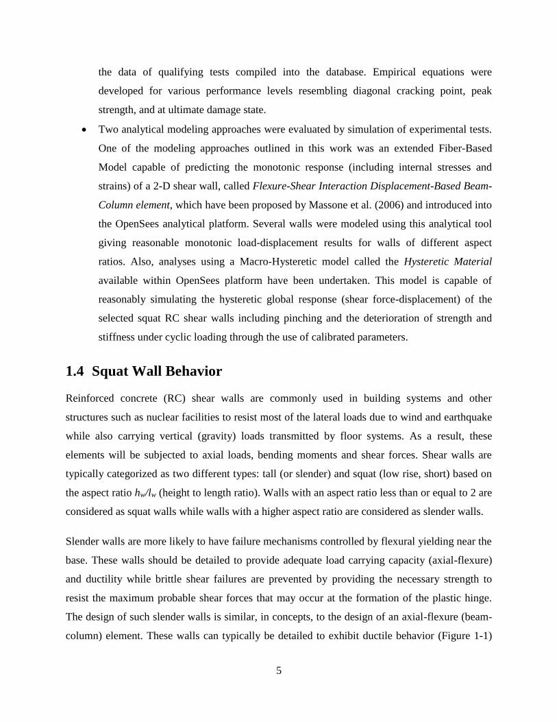
column) element. These walls can typically be detailed to exhibit ductile behavior (Figure 1-1)

6

under cyclic lateral loading since they are typically designed to fail by flexure (Paulay and

Priestley, 1992).

Figure 1-1. Stable hysteretic behavior of a ductile wall structure (Paulay and Priestley, 1992).

Due to their geometry, squat shear walls tend to have shear-dominant failure mechanisms.

Generally, the flexural demand of such walls is relatively low when compared to the flexural

capacity provided by the section. Therefore, it may be difficult or not economically feasible to

prevent a shear failure by matching the shear resistance with the flexural strength as in the case

of slender walls (Paulay and Priestley, 1992). Thus, typical squat walls are prone to undesirable

(non-ductile) shear failures characterized by sudden loss of strength and stiffness under lateral

cyclic loading (Figure 1-2). The main shear failure mechanisms associated with squat walls are

diagonal tension, diagonal compression, sliding shear or a combination of the aforementioned

(Paulay and Priestley, 1992; Gulec and Whittaker, 2009).

Typical cross section shapes found on experimental tests are shown in Figure 1-3. Squat walls

with boundary elements (barbell or flanged) can usually achieve higher peak shear strength than

7

similar walls of rectangular cross sections (ASCE 43-05). This effect may be attributed to the

additional reinforcement and wall web confinement provided by the boundary elements.

Figure 1-2. Hysteretic response of a structural wall controlled by shear (Paulay and Priestley, 1992).

(a)

(b)

(c)

Figure 1-3. Typical wall cross sectional shapes: (a) rectangular cross section (adapted from Whyte and

Stojadinovic, 2013); (b) barbell cross section (adapted from Matsui et al., 2004); (c) flanged cross section

(adapted from Barda, 1972).

Walls with intermediate aspect ratios between 1.5 and 3.0 (often called medium-rise or moderate

slenderness shear walls) tend to show a behavior influenced by both shear and flexure (ASCE

8

41-06). Thus, shear walls with aspect ratio higher than 3.0 can be considered as slender

meanwhile walls with aspect ratio less than 1.5 can be considered as squat. Engineering

judgment must be used when evaluating walls with intermediate aspect ratio since even when a

shear capacity higher than the shear force corresponding to flexural yielding is provided, the wall

can exhibit a shear failure when subjected to cyclic loading. This kind of failure can occur when

the wall initially yields in flexure (denoted by horizontal cracking and reinforcement yielding

initiated at the wall flexural tension zones or boundary elements) but then, the shear strength is

degraded after various displacement cycles falling below the shear force associated with flexural

yielding (Gulec and Whittaker, 2009). The shear failure leads to a sudden degradation of

strength, stiffness and ductility, diminishing the wall energy dissipation capacity which is one of

the main resources for earthquake resistance when the structure is designed to perform in the

nonlinear (inelastic) range. This type of failure is often referred in the literature as to mixed

flexure-shear failure.

1.5 Failure Modes of Squat Reinforced Concrete Walls

This work focuses in the behavior of squat shear walls with aspect ratio less than or equal to 1.5.

For such walls, the mechanisms of shear resistance observed from extensive studies of reinforced

concrete beams and slender walls are not entirely applicable due to the significant differences in

relative dimensions, boundary conditions, and the shear load application mechanism (Paulay et

al., 1982). Based on the studies of Barda (1977) and Paulay et al. (1982), among other

researchers who studied the behavior of squat walls, it was found that besides the contribution of

horizontal shear reinforcement, a large amount of the shear applied at the top of the wall is

transmitted directly to the foundation by means of diagonal compression. This load transmission

mechanism leads to the shear failure mechanisms mentioned before which will be briefly

discussed in the following sections.

1.5.1 Diagonal Tension Failure

This failure mechanism is likely to occur when the wall has insufficient horizontal reinforcement

and is characterized by one or more wide corner-to-corner crack as shown in Figure 1-4(a). This

mechanism is initiated with the tension cracking of concrete in a principal state of stress;

thereafter the steel yields significantly resulting in large crack widths and loss of the shear

9

friction resistance. The inclination of the crack is highly affected by wall geometry and the load

distribution at the top of the wall. The presence of a stiff element such as a beam induces the

formation of a corner-to-corner crack. The diagonal crack may also develop in a steeper angle

(Figure 1-4b). This diagonal crack may result in failure if there is no way of redistributing the

excess shear load to the rest of the wall top edge. A top slab or beam capable of redistributing the

shear can suppress this premature failure after the crack formation. The damage associated with

this failure mode is typically concentrated in one or few cracks which develop in both directions

of loading (if loading is cycled) forming an X-pattern.

(a) (b)

Figure 1-4. Diagonal tension failure modes (Paulay et al., 1982): (a) corner-to corner crack; (b) steep-

angle crack.

1.5.2 Diagonal Compression Failure

Diagonal compression failure could take place when a diagonal tension failure is prevented

through an adequate horizontal reinforcement and large shear stresses are induced. The

characteristic widespread crack pattern of this failure mode is shown in Figure 1-5a. Such

mechanism is produced when stresses in diagonal compression struts become large enough as to

exceed the concrete crushing strength. During cyclic loading interconnecting diagonal shear

cracks develop in the two opposite directions and progressively degrade the concrete strength,

which leads to concrete crushing at considerably lower shear load levels (Paulay et al., 1982). It

has been observed (Figure 1-5b) that the crushing frequently extends through the length of the

wall within few cycles of inelastic response (Paulay and Priestley, 1992). Walls with boundary

elements are more prone to diagonal compression failure than walls with rectangular sections,

10

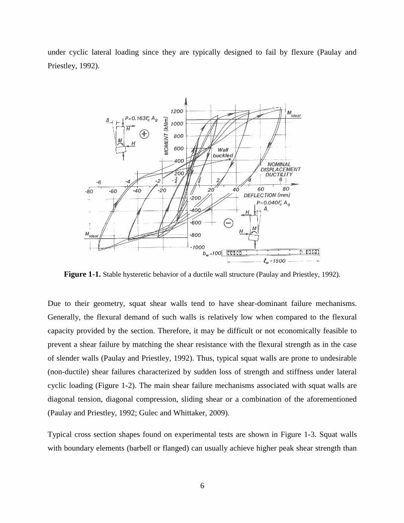
since they can produce higher flexural strength, thus increasing the shear demand on the web

(Gulec and Whittaker, 2009).

(a) (b)

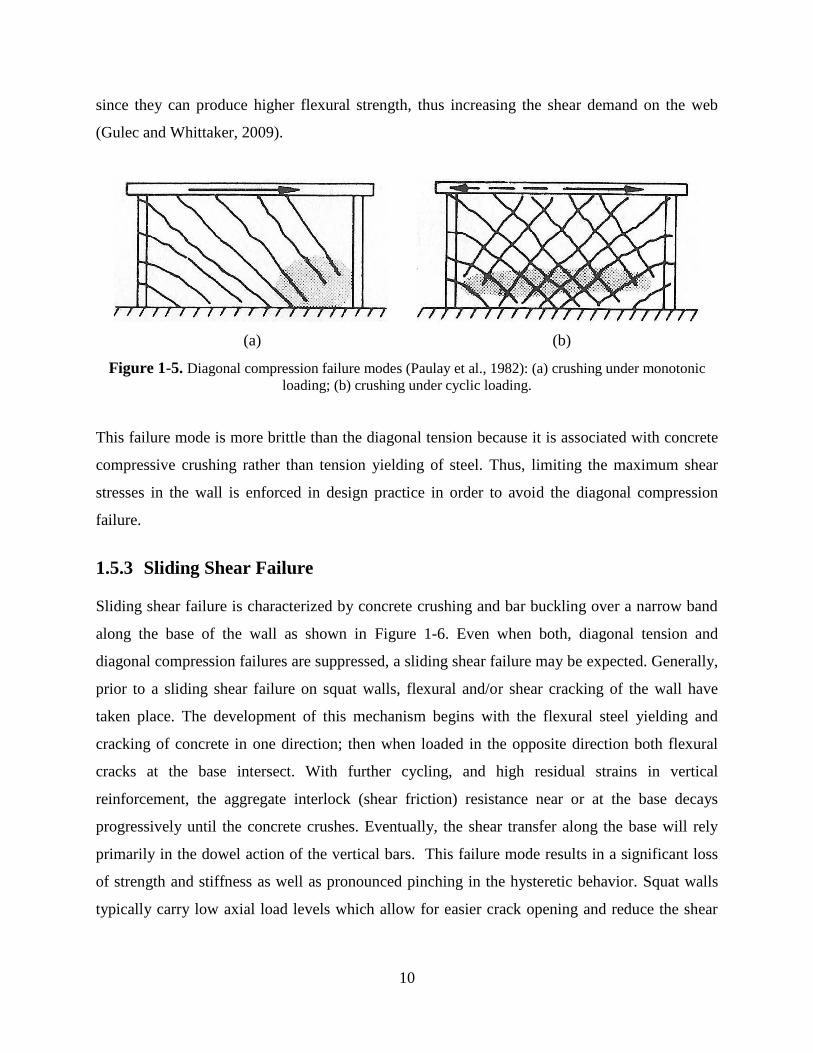
Figure 1-5. Diagonal compression failure modes (Paulay et al., 1982): (a) crushing under monotonic

loading; (b) crushing under cyclic loading.

This failure mode is more brittle than the diagonal tension because it is associated with concrete

compressive crushing rather than tension yielding of steel. Thus, limiting the maximum shear

stresses in the wall is enforced in design practice in order to avoid the diagonal compression

failure.

1.5.3 Sliding Shear Failure

Sliding shear failure is characterized by concrete crushing and bar buckling over a narrow band

along the base of the wall as shown in Figure 1-6. Even when both, diagonal tension and

diagonal compression failures are suppressed, a sliding shear failure may be expected. Generally,

prior to a sliding shear failure on squat walls, flexural and/or shear cracking of the wall have

taken place. The development of this mechanism begins with the flexural steel yielding and

cracking of concrete in one direction; then when loaded in the opposite direction both flexural

cracks at the base intersect. With further cycling, and high residual strains in vertical

reinforcement, the aggregate interlock (shear friction) resistance near or at the base decays

progressively until the concrete crushes. Eventually, the shear transfer along the base will rely

primarily in the dowel action of the vertical bars. This failure mode results in a significant loss

of strength and stiffness as well as pronounced pinching in the hysteretic behavior. Squat walls

typically carry low axial load levels which allow for easier crack opening and reduce the shear

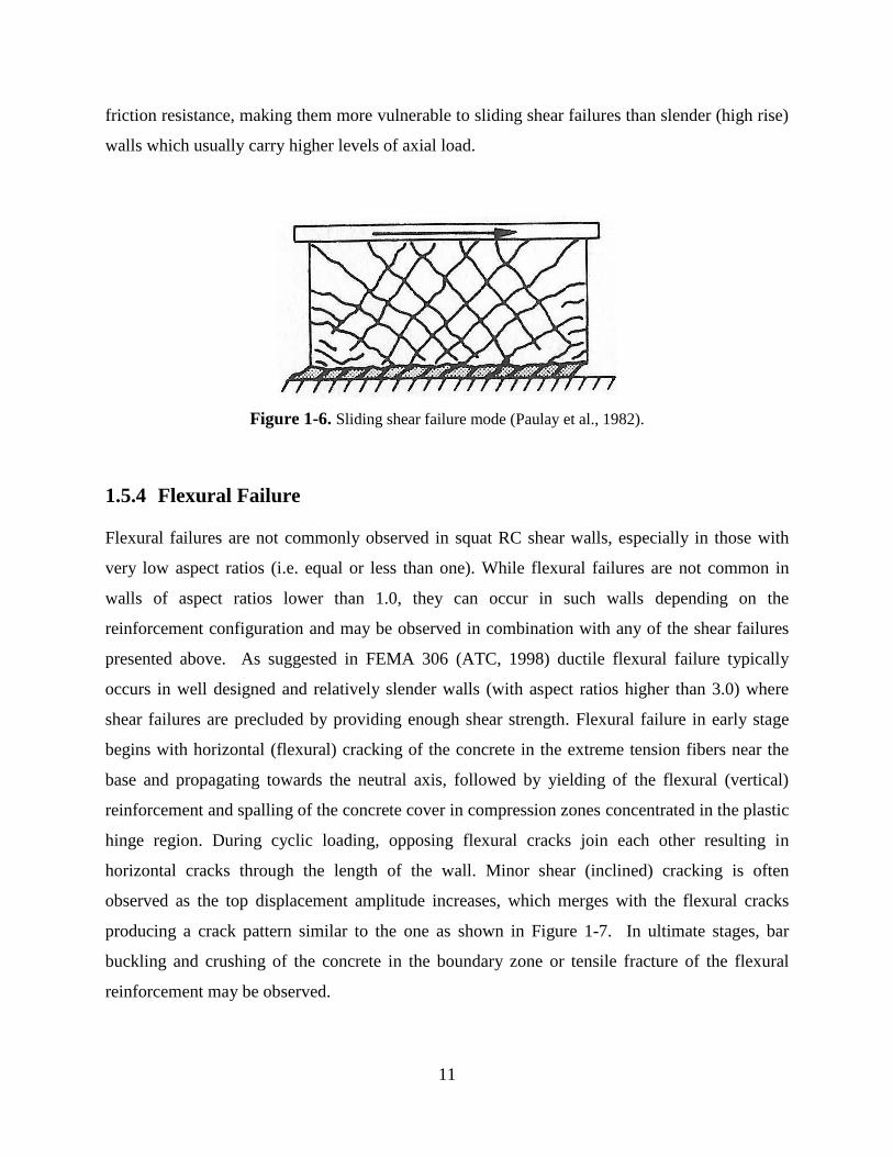
11

friction resistance, making them more vulnerable to sliding shear failures than slender (high rise)

walls which usually carry higher levels of axial load.

Figure 1-6. Sliding shear failure mode (Paulay et al., 1982).

1.5.4 Flexural Failure

Flexural failures are not commonly observed in squat RC shear walls, especially in those with

very low aspect ratios (i.e. equal or less than one). While flexural failures are not common in

walls of aspect ratios lower than 1.0, they can occur in such walls depending on the

reinforcement configuration and may be observed in combination with any of the shear failures

presented above. As suggested in FEMA 306 (ATC, 1998) ductile flexural failure typically

occurs in well designed and relatively slender walls (with aspect ratios higher than 3.0) where

shear failures are precluded by providing enough shear strength. Flexural failure in early stage

begins with horizontal (flexural) cracking of the concrete in the extreme tension fibers near the

base and propagating towards the neutral axis, followed by yielding of the flexural (vertical)

reinforcement and spalling of the concrete cover in compression zones concentrated in the plastic

hinge region. During cyclic loading, opposing flexural cracks join each other resulting in

horizontal cracks through the length of the wall. Minor shear (inclined) cracking is often

observed as the top displacement amplitude increases, which merges with the flexural cracks

producing a crack pattern similar to the one as shown in Figure 1-7. In ultimate stages, bar

buckling and crushing of the concrete in the boundary zone or tensile fracture of the flexural

reinforcement may be observed.

12

Figure 1-7. Typical flexural cracking pattern at a moderate stage of damage (ATC, 1998).

1.6 Review of Experimental Studies

In the past, the performance of squat walls has been compared to that of deep beams but their

behavior is considerably different in terms of the load application and load resisting mechanism

through arching action. Therefore, research findings from deep beam testing are not directly

applicable to shear walls. Considerable experimental research on squat RC shear walls have been

performed worldwide since 1950s yielding significant amount of experimental data. Most of

these tests have been carried out at the component level, as isolated shear walls with a cantilever

setup, where the load is applied to the wall panel through a rigid element at the top of the wall

simulating a slab or beam of a structure and transferred through the wall panel to a stiff concrete

foundation beam anchored to a strong floor. Other studies have tested specimens with fully

restrained rotation at the top of the wall. These conditions may be representative of coupling

beams and wall-piers where rotation is restricted at both ends instead of a cantilever shear wall

within a structure, therefore they are not included in this study. In earlier times, most of the tests

were conducted using monotonically increasing lateral load and using small scale specimens.

Due to the size limitations, several of these small scaled specimens were constructed using

cementitious mixes without coarse aggregates. Concrete containing a well distributed aggregate

matrix, including coarse aggregates can behave differently to a mortar-like mix without coarse

aggregates under the action of stresses. Therefore, these small scale specimens may not be

representative of the actual construction practices and are not included in the present study.

13

Eventually, quasi-static cyclic loading and larger scale specimens were commonly used. Also,

quasi-static hybrid-simulated earthquake loading and dynamic earthquake loading tests have

been carried out in more recent research. The main characteristics of the specimens are the type

of cross section (rectangular or flanged/barbell), aspect ratio (height to length ratio),

reinforcement quantities, concrete and steel strength and presence of coexisting axial load. A

summary of each experimental program included in the database have been considered within

this section.

Barda (1972)

A total of eight walls with heavily reinforced flanges were tested without axial loading. All walls

had the same cross sectional dimensions: 190 cm length, 10 cm thick web and flanges and 60 cm

wide flanges. All walls were over-designed for flexure in a way that shear failure modes were

expected. Two of the walls were tested under monotonic loading while other six were subject to

reversed cyclic loading. Shear span-to-length ratios ranged between 0.25 and 1.0. Barda (1972)

reported that load reversals produced around 10% peak shear strength reduction when compared

to a companion specimen loaded monotonically. This study also concluded that both the

horizontal and the vertical steel were effective providing shear strength and the proportion varies

with aspect ratio. It was reported that horizontal reinforcement did not contribute to shear

strength for walls with aspect ratios of 0.25 and 0.5 while vertical reinforcement was effective

providing shear strength for those walls. Horizontal reinforcement improved wall behavior by

inducing the formation of more distributed crack pattern and reducing crack widths on specimens

with aspect ratios of 0.25 and 0.5. Effectiveness of vertical reinforcement in lateral strength

decreased for the wall specimen with aspect ratio of 1.0. Therefore, recommendations were given

on minimum reinforcement quantities in vertical as well as in horizontal direction. Decreasing

wall aspect ratio (or shear span-to-length ratio) produced higher shear strengths. Well confined

boundary elements helped in maintaining a gradual decrease in post-peak residual strength

instead of sudden failure. Barda’s design recommendations with slight modifications are still

used on the design provisions for squat walls with flanged or barbell cross sections on the ASCE

43-05 standard.

14

Alexander et al. (1973)

Alexander’s group tested a series of five walls at McMaster University at Ontario, Canada. The

wall specimens had rectangular cross section, thickness of 10 cm, height of 137 cm and aspect

ratios ranging between 0.5 and 1.5. Three of the walls had axial compressive load which ranged

from 4.6% to 9.3% of the gross axial strength. Four of the panels included additional

reinforcement at the foundation beam to panel interface (starter bars) which was reported to

dramatically change the failure mechanisms and the force-displacement characteristics. The tests

also aimed to evaluate the effects of axial load and wall aspect ratio. They found that axial loads

increase the lateral load carrying capacity and improves stiffness degradation but reduces panel

ductility. Also, higher panel aspect ratios produced lower maximum shear stresses.

Hirosawa (1975)

Hirosawa described a compilation of past experimental studies of RC shear walls under

combined axial, shear and flexural loading carried out in Japan. Hirosawa’s database included

walls with rectangular, flanged and barbell cross sections. Experimental setup and main

specimen properties along with experimental results have been listed on Hirosawa’s report.

Cardenas et al. (1980)

Seven walls with rectangular cross-sections and aspect ratio of 1.0 (M/Vlw =1.08) and without

axial load were tested. Six of the walls were loaded monotonically and only one was subject to

cyclic load. The main objective of this experimental program was to investigate the contribution

of vertical and horizontal reinforcement on the shear strength. It was reported that both vertical

and horizontal reinforcement contributed to the shear strength and effectively restrained crack

widths of squat walls with aspect ratio of 1.0 under lateral loading. However, variation of

effectiveness of vertical and horizontal reinforcement with aspect ratio was not investigated. It

was also reported that the cyclically loaded specimen yielded lower shear strength than an

identical specimen loaded monotonically.

Endo (1980)

Twenty wall specimens with barbell cross section were tested in Japan under this experimental

program. Three specimens were tested under monotonic lateral load while reversed cyclic

15

loading was applied to the others. Main parameters were: aspect ratio of 0.78 and 1.22 (M/Vlw of

0.83 and 1.28), wall thickness ranging from 5 cm to 10 cm, boundary element reinforcement

ratio varying from 0.81% to 2.44%, wall web reinforcement ratio ranging from 0.23% to 0.71%

and variations in boundary element confinement. Coexisting axial loads were applied to all walls

which resulted in an axial load ratio ranging from 4.0% to 9.7%. One of the main findings from

these tests was that the ductility of walls tested monotonically is different from the walls tested

cyclically. By comparison of companion specimens tested under reversed-cyclic and monotonic

loading, it was observed that monotonically loaded specimens can reach moderately higher

strength and considerably higher drifts levels before failure. In concurrence the findings of other

researchers, as the shear span-to-length ratio increases, the strength decreases but the

displacement capacity (drift ratio) increases. The longitudinal boundary element reinforcement

contributed significantly to the shear strength of the walls. Also, their tests reveal that the hoop

reinforcement ratio of the boundary elements does not contribute significantly to the shear

strength, but the higher confinement allows the walls to sustain the loads to higher drift ratios

after peak strength as well as to minimize post-peak strength degradation.

Hernández (1980)

A total of twenty-two small scaled wall specimens including rectangular, flanged and barbell

cross sections were tested in Mexico. All specimens had a coexisting axial load corresponding to

7% of Ag f’c. While the scale of the specimens in this experimental program was very small

(thickness of 2.5 cm), some important findings on general behavior were noted. Cyclic load

reversals resulted in an average of 15% strength reduction when compared to similar

monotonically loaded specimens. Lower aspect ratios resulted in increased shear strength, but

reduced displacement capacities. Shear critical walls resulted in poor hysteretic behavior and

progressive deterioration of strength under reversed cyclic loading.

Synge (1980)

Synge’s group worked under the supervision of Dr. Thomas Paulay and Dr. Nigel Priestley at the

University of Catenbury, New Zealand. Four walls of 300 cm long, 150 cm high and 10 cm thick

were tested under reversed cyclic loading. Two of the specimens had rectangular cross section

and other two had flanges. One wall of each cross section type included diagonal reinforcement

16

which was found to reduce sliding shear and improve hysteretic behavior. Synge’s group

reviewed failure mechanisms of squat walls with particular attention on sliding shear, as it was

deemed that all squat walls with zero or very low axial load levels are prone to this failure mode.

Saatcioglu (1985-1994)

Dr. Murat Saatcioglu directed the work of Wiradinata (1985), Pilette (1987), Wasiewicz (1988)

and Mohamaddi-Doostdar (1994) at the University of Toronto and the University of Ottawa,

Canada. For a series of walls tested without axial load (wall 1 to wall 8), the concrete

compressive strength ranged from 22 to 45 MPa, the aspect ratio varied from 0.25 to 1.0 (M/Vlw

between 0.33 and 1.09). Vertical reinforcement ratios ranged from 0.7 to 1.15, while horizontal

reinforcement ratios ranged from 0.21 to 1.15. All walls had rectangular cross sections

measuring 10 cm x 200 cm, except Wall 8 which length was 150 cm. Wasiewicz’s group tested

two specimens including additional reinforcement at the foundation to wall interface, intended to

control sliding shear. These specimens with an additional interface reinforcement showed

significantly different behavior to similar companion specimens tested by Wiradinata (1985).

Their main findings, as described on their experimental program, have been summarized as

follows:

Wall aspect ratio is a key factor in wall strength and behavior.

While all wall specimens showed sliding shear damage (with the exception of walls with

additional joint reinforcement), walls with aspect ratios below 0.5 are more prone to

sliding shear failure.

Specially detailed additional reinforcement at construction joint effectively suppressed

sliding shear failure.

Walls with lower aspect ratios develop higher shear strength.

Walls with aspect ratios of 0.5 and below showed predominant shear behavior.

Walls with aspect ratios between 0.75 and 1.0 showed equally important deformation

components for shear and flexure.

Chiba et al. (1985)

A series of 20 shear wall specimens without openings and 13 specimens with web openings were

tested in Japan. The main parameters of the study were the reinforcement ratio of the wall

17

(ranging from 0 to 2.76%), the shear span-to-length ratio (M/Vlw ranging from 0.35 to 0.70), the

axial load ratio (ranging from 0 to 12.4%), and the presence and arrangement of openings. All

wall specimens were tested under reversed cyclic loading and had thickness of 8 cm, boundary

elements measuring 30 cm x 30 cm and total wall length of 230 cm. Gulec and Whittaker (2009)

reported the results of these and several other wall experiments collected from Japanese literature

which are part of a Japanese research program called “Load-Deflection Characteristics of

Nuclear Reactor Building Structures”. Experimental results for a total of 29 wall specimens

without openings were collected from this program which are included in the database under the

following researcher names: Chiba, Yagishita, Fukuzawa, Hatori and Taga. General findings

were well in agreement with the reported tendencies from other researchers as the shear strength

increased with increasing axial loads, increasing web reinforcement and decreasing shear span-

to-length ratio (or conversely aspect ratio). It was also found that the specimens with higher web

reinforcement ratios, which had closer bar spacing, showed more uniform and closely spaced

diagonal cracks than those with lower reinforcement ratios. As reported by the authors,

contribution of web reinforcement in shear strength was observed even on reinforcement ratios

higher than 1.2% which was considered as maximum effective reinforcement in the Architectural

Institute of Japan standards.

Hwang and Sheu (1988)

An experimental program on low-rise shear walls was conducted by M. S. Sheu at the National

Cheng-Kung University at Taiwan, China. Gulec and Whittaker (2009) collected and reported

the results of twenty-seven walls with rectangular cross section and seventeen walls with barbell

cross section tested by Sheu. As reported by Gulec, shear span-to-length ratio (M/Vlw) ranged

between 0.65 and 1.90, four walls with rectangular cross sections were tested with a coexisting

axial force of 0.12 Ag f’c and one wall with barbell cross-section was tested with a coexisting

axial force of 0.063 Ag f’c. Nineteen walls were tested under monotonic lateral load, 3 walls were

subjected to repeated (one direction) loading, and 22 walls were tested under reversed cyclic

loading. Analyzing the test results, it can be noted that: as aspect ratio decreases higher strengths

are attained, the presence of axial loads produced a significant increment in shear strength, and

both vertical and horizontal web reinforcement had a significant contribution in shear strength

for the range of aspect ratios tested.

18

Saito et al. (1989)

Nine flanged specimens were tested with f’c ranging from 23.5 MPa to 41.2 MPa, fy of 369 MPa,

equal horizontal and vertical reinforcement ratios ranging from 0.90% to 1.69%, shear span-to-

length ratio M/Vlw of 0.5 and 1.0, Axial load ratios P/ Ag f’c ranging from 2.38% to 8.33%. The

main objective of the study was to evaluate the applicability of design practices used for walls

with normal strength concrete of that time (around 24 MPa) to walls with higher strength (around

35 MPa). The effects of axial loads, reinforcement ratios and aspect ratio of the wall were similar

to the observed tendencies from other researchers.

Sato et al. (1989)

Twenty-two flanged walls were tested. These walls have the following properties: f’c ranging

from 24.5 to 44.6 MPa, fy from 296 to 528 MPa, equal horizontal and vertical reinforcement

ratios ranging from 0.45% to 1.60%, shear span-to-length ratio ranging from 0.6 to 1.2, and axial

load ratios ranging from 4.5% to 8.2%. The main purpose of these tests was to use different steel

grades and reinforcement ratios, but varying only the product of the two (ρfy) as the web

reinforcement parameter. The study concluded that the load-deflection relationship and failure

mechanisms of such squat RC walls are directly related to the product of reinforcement ratio and

reinforcement yield strength regardless of the grade of steel. As of that time, Japan standards

restricted the shear reinforcement yield strength to a maximum of 300 MPa. The authors

recommended to allow the use of higher yield strength up to 500 MPa for the shear

reinforcement in the design practice, as the walls behavior and performance resulted to be similar

to those designed using lower yield strength.

Maier (1991)

Seven walls with flanged cross section and three walls with rectangular cross section were tested.

All wall specimens had aspect ratio hw/lw = 1.02 (M/Vlw = 1.12), 120 cm height and 10 cm web

thickness. One flanged wall (S8) had an opening in the compression zone at the bottom of the

wall. All walls were tested under combined constant axial load and increasing shear loading.

Only two flanged specimens (S5 and S7) were tested under reversed cyclic loading. Concrete

compressive strength ranged from 29.2 to 37.3 MPa while axial loads ranged from 6.8% to

27.9%. The study revealed that vertical reinforcement was effective in providing shear strength

19

while horizontal reinforcement had marginal contribution to lateral strength on the tested walls.

Higher axial loads and higher vertical reinforcement ratios produced higher strength but

decreased ductility. Horizontal reinforcement contributed to the improvement of wall

deformation capacity. Cyclically loaded specimens with low axial load did not show significant

change in behavior when compared to their monotonic companion specimens. However,

decreased strength was observed on cyclically loaded walls with higher axial loads.

Rothe (1992)

Gulec and Whittaker (2009) collected and reported the test results of shear walls tested by Rothe.

As reported by Gulec and Whittaker, six walls with barbell and five walls with rectangular cross-

sections were tested. All walls had shear span-to-length ratio (M/Vlw) of 1.5. Three walls were

subject to constant axial forces ranging from 0.065 Ag f’c to 0.096 Ag f’c. Five walls were tested

under reversed cyclic loading, one wall was loaded monotonically, and 5 walls were tested under

dynamic earthquake simulated loads.

Seki et al. (1995)

Six flanged walls were tested by pseudo-dynamic (hybrid simulated) loading method. Their

objectives were to characterize the lateral force-displacement behavior and equivalent viscous

damping of the walls, and to verify the feasibility of hybrid simulation testing for squat shear

walls. Their test specimens had shear span-to-length ratios (M/Vlw) of 0.6, 0.8 and 1.0. All

specimens had uniform reinforcement ratios of 1.2% (vertical and horizontal) and thickness of 75

mm in both, web and flanges. All walls had similar compressive strength ranging from 28.9 to

31.6 MPa at the age of testing. Steel yield stress ranged from 349 to 381 MPa. Axial load ratio

was varied from 0% to 3.5%. They found that the shear displacement component was

predominant in all the tested specimens ranging from 90% to 60%. The shear displacement

component percentage decreased as the shear span-to-length ratio increased. Lateral strength

tended to increase with application of axial loads, as well as with decreasing shear span-to-length

ratio. Equivalent viscous damping ratio generally fell between 2% and 6%, but was highly

scattered for small displacement demands and for near-failure displacements. Equivalent viscous

damping showed a tendency to increase at high displacement demands. The authors concluded

20

that the pseudo-dynamic loading was a feasible method to simulate seismic response of squat

shearwall structures.

CNSI/NUPEC (1996)

In 1991, the Japanese Nuclear Power Engineering Corporation (NUPEC) conducted tests in two

flanged wall specimens (U-1 and U-2) under dynamic excitation in one direction. These test

results were published on 1996 by the OECD – NEA Committee on the Safety of Nuclear

Installations (CSNI). Both wall models were identical and were subjected to the same dynamic

input records to verify the reproducibility of the tests. The response of both walls was reported to

be very similar in terms of force, deformation, crack pattern, and failure mode. Wall specimens

were 202 cm high, 310 cm long, with 10 cm x 298 cm flanges and web thickness of 7.5 cm. Web

reinforcement ratio was set to1.2% and concrete strength 28.6 MPa. Axial load was applied by

additional mass attached to the top slab with a resultant axial load ratio of 3.9% of f'cAg. The

study aimed to provide data on the seismic response characteristics of squat RC shear walls

typically found in nuclear power plants under loading levels that ranged from the essentially

elastic state to the elasto-plastic ultimate state. Their data were used to develop and calibrate

analytical computer models by allowing to be utilized by several organizations and hosting

workshops under a program named “Seismic Shear Wall International Standard Problem”

(SSWISP).

Kabeyasawa and Hiraishi (1998)

A total of twenty-one high-strength reinforced concrete shear walls specimens were tested under

reversed cyclic loading as part of a national research project in Japan. Concrete with compressive

strength ranging from 54.6 MPa to 137.5 MPa, and reinforcing steel with yield strength ranging

761 MPa to 1,395 MPa were used. All specimens had barbell cross sections with 8 cm web panel

thickness, 20 cm x 20 cm confined boundary elements and total wall length of 170 cm. Web

reinforcement ratios varied from 0.20% to 1.45%, and axial load ratios ranging from

approximately 10% to 14% of Agf’c were applied to the wall specimens. The purpose of the

program was to investigate the feasibility of the design and construction of reinforced concrete

shearwall structures using ultra-high strength materials.

21

Salonikios et al. (1999)

The research program involved testing of eleven rectangular cross section walls with aspect

ratios of 1.0 and 1.5 (M/Vlw = 1.1 and 1.6) under reversed cyclic loading. Two specimens were

tested with axial load corresponding to 7% Ag f’c while the other nine had zero axial load. All

wall specimens had adequately confined reinforcement at the boundary element zones. Four of

the specimens (two of each aspect ratio) included diagonal reinforcement. Pilot specimen MSW2

was reported to show out-of-plane buckling behavior due to the lack of lateral restrain in the test

setup. Specimen MSW1 is considered flexure controlled after cross section analysis. The shear

deformation components (sliding + web shear) contributed between 20% to 80% to the total wall

deformation and usually increased with the ductility level. Sliding shear deformations increased

substantially for displacement ductilities above 2.5. For most walls, sliding shear deformations

were significantly higher than the diagonal (web distortion) shear deformations. Walls with

diagonal reinforcement showed improved hysteretic behavior with higher energy dissipation and

reduced sliding at the base. Compressive axial load had a favorable effect in reducing sliding

shear. Walls with lower aspect ratio showed significantly higher sliding and strength

degradation. Axially loaded members as well as those with increased reinforcement ratios

showed less strength degradation.

XiangDong (1999)

The experimental program at the University of Houston, Texas included the testing of thirteen

framed wall specimens and a frame specimen without wall panel. Specimens named FSW-1,

FSW-2 and FSW-3 had different shortcomings and served as pilot specimens to test and improve

the experimental setup. Wall specimen FSW-11 was also reported to fail prematurely and

therefore is not included in the database on this research. All the specimens had the same

dimensions and frame element longitudinal reinforcement: frame elements were 152.4 mm x

152.4 mm, wall thickness 76.2 mm and 914.4 x 914.4 mm of clear wall panel. Concrete target

compressive strength was 55 MPa. However, it varied from 48.3 MPa to 57.1 MPa. Main

parameters were the axial load ratio (varying from 1.3% to 9.3%), web reinforcement ratio

(varying from 0.23% to 1.11%) and hoop spacing on the frame members. The authors reported

that when the axial load ratio increased from about 1.4% to 4.5%, the lateral shear strength

increased significantly by 40%. However, when axial load ratio increases from about 4.5% to

22

8.5%, the strength increased by only 13%. In contrast, varying the steel ratio of the wall panel

from 0.25% to 0.5%, did not change the lateral strength appreciably but when panel

reinforcement ratio was increased from 0.5% to 1.0%, the shear strength was improved by an

average of 25%. As the panel reinforcement ratio increased, the spacing and width of cracks

decreased and were more evenly distributed in the panel resulting in better ductility and

hysteretic behavior. When minimum panel reinforcement was used, the diagonal tension failure

mode - characterized by one or few substantially wide diagonal crack in the panel - was predominant.

Thus, the authors suggested that a minimum reinforcement ratio of 0.5% would be more

appropriate. Increasing boundary element confinement (hoops) helped to prevent crushing of

concrete and longitudinal bar buckling at the boundary elements, and reduced pinching effect. Shear

displacement component ranged from 68% to 95% of the total displacement.

Palermo and Vecchio (2002)

Two identical flanged wall specimens (DP1 and DP2) were tested under reversed cyclic loading.

Axial load of 5.45% of f’cAg was applied to specimen DP1 while specimen DP2 had no axial

load. These wall specimens were similar to NUPEC’s dynamic loaded specimens. Wall

specimens were 202 cm high, 307.5 cm long, with 9.5 cm x 304.5 cm flanges and web thickness

of 7.5 cm. Web reinforcement ratio was set to 0.73% and 0.79% in the horizontal and vertical

directions, respectively. Concrete compressive strength was 21.7 MPa and 18.8 MPa for

specimens DP1 and DP2, respectively. Test results show that axial load has a significant effect

on wall behavior. In their case, a small amount of axial load (5.45% of f’cAg) significantly

improved shear strength. In contrast to typically observed behavior on other experiments, the

wall with axial load showed improved ductility and energy dissipation characteristics. The

authors attributed this non-typical ductility behavior to the fact that both walls showed different

failure modes. The wall without axial load showed sliding shear plane formed at the top of the

wall web (possibly due to weaker concrete near the top of the wall section) while the wall with

axial load showed web crushing failure mechanism.

Matsui et al. (2004)

Two identical specimens with barbell cross section were tested at the University of Tokyo under

uni-directional dynamic shake table loading. Both specimens had a wall clear height of 180 cm,

23

web thickness of 8 cm, well confined boundary elements measuring 20 cm x 20 cm, web

reinforcement ratios of 0.40%, and axial load ratios of nearly 6.5% of Agf'c. Only the height from

the base to the top weight center of mass was changed on the two specimens which resulted in

shear span-to-length ratio (M/Vlw) of 1.38 and 1.76 for Wall-A and Wall-B, respectively. The

two specimens were subjected to equal series of scaled earthquake motion records. The failure

modes of both walls were different which shows the influence of the shear span-to-length ratio

on the response of these walls. Wall A, with lower shear span-to-length ratio, resulted in higher

shear strength and significantly higher shear deformation component. Wall B (M/Vlw = 1.76)

showed equally important flexural and shear deformation components, while for Wall A shear

deformation was about twice the flexural deformation.

Dabbagh (2005)

A series of six squat walls with barbell cross section and high strength concrete were tested

under reversed cyclic loading at the University of New South Wales, Sydney, Australia. All

specimens had the same dimensions with thickness of 7.5 cm, length of 100 cm and aspect ratio

of 1.0 (M/Vlw = 1.10). Five specimens were tested with axial load ratio of nearly 10% of Ag f’c

and one had no axial load. Boundary element reinforcement ratio was set to 6.43% while web

reinforcement ratios varied from 0.45% to 1.34%. Concrete compressive strength ranged from 83

MPa to 96 MPa, while reinforcement yield strength varied from 498 MPa to 536 MPa. They

observed that, at this aspect ratio, an increase only in the vertical reinforcement ratio led to an

increase in peak shear strength but this effect was not as significant as in normal strength

concrete walls. Horizontal reinforcement ratio did not have a significant effect on peak strength

but caused an increase in wall’s displacement capacity. Dabbagh’s group also found that the

axial load significantly increased peak shear strength, but at the same time reduced ductility.

Greifenhagen and Lestuzzi (2005)

Results of four lightly reinforced, reversed cyclic loading, rectangular cross section specimens

were reported. Axial load ranged from 2.2% to 9.4% of Ag f’c and aspect ratio of 0.57 (M/Vlw =

0.69 to 0.76). Vertical and horizontal reinforcement ratios were set to 0.003. Concrete strength

ranged from 20 MPa to 51 MPa. Specimens M1 and M2 were excluded from database since the

actuator reached the maximum capacity of 200 kN during the test, and the axial load level had to

24

be reduced in order to achieve strength degradation of the specimen at higher displacement

levels. Specimen M3 was deemed to be controlled by flexure after cross section analysis. Shear

deformation components (sliding + shear distortion) contributed between 20% to 47% (average

30%) to the total deformation, depending on the ductility level. The portion of total deflection

due to flexure decreased as the lateral displacement increased, whereas sliding portions generally

increased as ductility and drift increased. Higher axial loads prevented the sliding shear failure

mode and thus, diagonal tension failure was induced because the walls had low reinforcement

ratios. In the cases with lower axial loads, where sliding shear failure mode predominated,

damage was concentrated at the bottom area near the foundation and the horizontal

reinforcement became ineffective. Higher axial load ratios produced less drift capacity. By

comparing their test results with other tests from literature, the authors suggested that the drift

capacity of squat walls depends mostly on axial force ratio, vertical reinforcement arrangement,

and degree of restraining at the top of the wall. They also found that cantilever shear walls

without rotation restraints at the top are less susceptible to brittle shear failures than those with

fixed top end.

Akita et al. (2006)

Two wall specimens with barbell cross section were tested under coexisting axial and shear

loading. The two specimens were nominally identical to the specimens on the dynamic tests by

Matsui et al. (2004), but these were subjected to quasi-static reversed cyclic loading. The main

objective of their study was to compare the behavior of RC shear walls under quasi-static cyclic

loading and dynamic loading. In general, the lateral load-displacement characteristics and failure

modes observed on the quasi-static tests were similar to those of the dynamic tests.

Sanada and Kabeyasawa (2006)

Two companion walls with barbell cross-section were tested under reversed cyclic loading at the

University of Tokyo. Constant axial load corresponding to nearly 0.10 of Agf'c was applied to

both walls during testing. Both walls had web reinforcement of 0.25% on each direction, web

thickness of 8 cm, 140 cm clear height, 25 cm x 25 cm boundary elements and aspect ratio hw/lw

of 0.68. One of the specimens (Type-N) was built with normal base consisting of a stiff

continuous foundation beam, while the other (Type-S) had a special base split into four pieces.

25

Each piece of the base was individually anchored and equipped with a biaxial load cell to

measure the local shear and axial forces. The hysteretic behavior, cracking pattern and failure

mode were similar for both walls, and therefore, the split base specimen reproduced the behavior

of the normal specimen. The authors found that about 70% of the total lateral force was carried

around the boundary column on the compressive side at the shear failure damage state. At lower

damage state (i.e. onset of shear cracking) the compression boundary column region carried

around 40% of the total lateral force. The shear force transfer at the tensile boundary element

zone was negligible at all damage states, which was to be expected because the cracks on the

tensile side are open and shear friction forces cannot effectively develop. These observations

suggested that forces were mainly transferred in a diagonal compression strut mechanism as the

wall experienced higher demands.

Kuang and Ho (2008)

Kuang and Ho’s group tested 8 walls with aspect ratios of 1.0 and 1.5, rectangular cross section

of 100 mm x 1200 mm. The intent of their study was to evaluate the behavior of non-seismically

detailed squat walls and the effectiveness of improved confinement detailing to enhance ductility

of such walls for moderate earthquake hazard. Concrete strength ranged from 30.4 MPa to 37.7

MPa and steel yield strength was 520 MPa. Axial load ratios ranged from 10% to 30% of Ag f’c.

All specimens exhibited a flexural failure mode. The authors observed that providing

confinement at the wall boundary zones resulted in significantly higher ductility and improved

energy dissipation. This may be attributed to the added concrete confinement in the compression

zone and the prevention of outer bars buckling as the bars lateral support becomes more closely

spaced. In the same manner, addition of crossties throughout the cross-section of the wall panel

provided confining stresses to the entire section, and thus, it enhanced walls ductility, energy

dissipation as well as shear strength. Concentrating the longitudinal reinforcement at the

boundary zones resulted in increased flexural strength but marginal improvement in ductility and

energy dissipation. The increased flexural strength induced the formation of more diagonal shear

cracks on the wall panel.

26

Xiang (2009)

Five walls with aspect ratio of 1.0 (M/V/lw = 1.125) and three walls with aspect ratio of 1.5

(M/Vlw = 1.625) were tested under reversed cyclic loading at Nanyang Technological University

in Singapore. Six of the walls were subjected to axial loads corresponding to 5% of f’c Ag while

the other two were tested without axial load. All walls had the same cross section with a 200 cm

length, 12 cm web thickness and boundary elements measuring 15 cm x 30 cm. The

reinforcement arrangement was the same for all specimens. Web reinforcement ratio of 0.5% and

boundary element reinforcement ratio of 1.4% were used. Most of the wall specimens were cast

monolithically with the top beam and bottom foundation except for three wall spaecimens that

included a construction joint at the base. All wall specimens had lower yield strength

longitudinal reinforcement at the boundary elements and showed flexure-controlled failure

mode. Higher confinement of the boundary elements produced higher ductility, higher energy

dissipation, and less strength degradation. Walls with axial load ratio of 5% showed higher

strength and higher energy dissipation and less pinching behavior due to the reduction of sliding.

The presence of a construction joint at the wall base resulted in higher sliding displacements.

Stiffness characteristics did not appear to be affected by the boundary element confinement. The

authors found that walls stiffness is mostly influenced by the outermost (boundary element)

reinforcement, axial load and aspect ratio.

Terzioğlu (2011) – As reported by Gutiérrez (2012) and Opazo (2012)

Eleven squat wall specimens with rectangular cross section were tested under reversed cyclic

loading at the University of Bogaziçi, Turkey. All cross sections measured 12 cm x 150 cm.

Aspect ratios ranged from 0.33 to 1.0. Two of the wall specimens carried axial loads

corresponding to 5.1% and 9.9% of Ag f’c while the rest were tested without axial loads. Web

reinforcement ratios were either 0.34% or 0.67%. Boundary element reinforcement ratios varied

from 0% to 9.75%. Concrete strength varied from 19.3 MPa to 35 MPa and steel yield strength

varied from 437 MPa to 572 MPa. All specimens showed shear failure modes. Test results

showed that increasing boundary element reinforcement ratio can significantly increase the shear

strength of shear-dominated walls with aspect ratios as low as 0.5. The presence of axial loads

produced higher shear strengths. The authors noted that wall specimens with lower aspect ratios

reached higher strengths and had predominant shear deformation components, whereas the wall

27

with higher aspect ratio (1.0) showed equally important flexural and shear deformation

components. The authors also noted that the wall specimens with lower web reinforcement

ratios tend to fail in diagonal tension, while higher panel reinforcement ratio suppressed the

diagonal tension mechanism leading to either diagonal compression or sliding failure

mechanisms. Wall specimens with diagonal compression failures showed the most brittle

behavior.

Altin et al. (2013)

Altin’s group tested five shear-deficient walls with aspect ratio of 1.5 (M/Vlw = 1.65) and 100

mm X 1000 mm rectangular cross section. The aim of their study was to investigate the effect of

different shear strengthening configurations using carbon fiber reinforced polymer (CFRP). One

reference specimen without CFRP reinforcement and other four specimens with CFRP

strengthening were tested. Steel yield strength ranged from 325 MPa to 425 MPa and concrete

strength was around 15.5 MPa. Walls had considerable concentrated longitudinal reinforcement

at the edges with no confining hoops and sub-minimum reinforcement ratios of 0.15% and

0.18% in the horizontal and vertical directions, respectively. No axial loads were applied to the

specimens. The reference specimen showed a diagonal tension shear failure mode with typical

wide and concentrated cracks along both of the diagonals. This failure mode was to be expected

due to the low panel reinforcement ratios and suppression of flexural failure by the boundary

longitudinal reinforcement. The CFRP strengthened specimens attained considerably higher

strength, ductility and energy dissipation.

Carrillo and Alcocer (2013)

This experimental program carried out in Mexico involved the testing of 39 isolated rectangular

cross section walls. The walls were full scale (10 cm thick and 250 cm height) models of typical

walls found in housing construction in Latin American countries. Four specimens had large web

openings representative of windows and doors. The tests included specimens with monotonic

loading, reversed cyclic, and dynamic loading. Aspect ratios were set to 0.44, 1.0 and 1.94.

Twelve of the specimens were reinforced with welded wire mesh made of cold drawn wire

having low tensile strain at fracture. On these specimens reinforced with wire mesh, the fracture

of web reinforcement led to brittle failure modes at lower displacements compared to specimens

28

with similar amount of mild rebar reinforcement. Therefore, these wall tests were not considered

in the database shown on Appendix A of this document. Three types of concrete were used,

namely, normalweight, lightweight and self-consolidating. Concrete strength ranged from 16.0

MPa to 24.7 MPa with the exception of few very low strength specimens whose concrete

strength was as low as 5.2 MPa. All specimens had confined boundary elements within the

rectangular cross section and were over-designed in flexure to induce shear failure modes. Equal

horizontal and vertical web reinforcement ratios ranging from 0% to 0.28% were used. Constant

axial stress of 0.25 MPa was applied to all specimens, which in general corresponded to axial

load ratios below 0.03f’cAg. Lower strength on reversed cyclic tests was noted when comparing

similar specimens tested under monotonic load from this program. The authors proposed a shear

strength predictive equation for walls with the characteristics found in one to two story concrete

housing based on calibration of the ACI 318 seismic provisions equation with their experimental

results. The authors found that shear strength increases as the shear span-to-length ratio (M/Vlw)

decreases; concrete strength corresponds to the diagonal tension strength of the wall; and that

web steel contributed to the shear strength, though it was not fully efficient. The authors

observed that the efficiency factor for the web steel ranged from 78% to 86%, but noted that as

the reinforcement ratios increased the efficiency factor decreased. The efficiency factor

accounted for the fact that the distribution of strains in the steel is not uniform along the wall

height and not all steel crossing the cracks reached yielding. Diagonal cracks usually grew wider

at the central panel zone and tended to be minimal near the top beam and bottom foundation.

Thus, authors deemed that yield potential is higher for the bars around the center of the panel.

Whyte and Stojadinovic (2013)

Two walls nominally identical to specimen SW3 (tested under cyclic loading at the University at

Buffalo) were tested under quasi-static hybrid-simulated earthquake loading at the NEES

facilities at Berkeley, California. Concrete compressive strength at day of testing was 35.5 MPa

and 37.3 MPa for Wall 1 and Wall 2, respectively. Reinforcement yield stress was 464 MPa.

Equal horizontal and vertical reinforcement ratios of 0.71% were used. Neither wall had axial

loading. By comparison of global responses of the walls tested at Berkeley and the nominally

identical wall tested at Buffalo, the authors observed that the responses were very similar, and

deemed that the quasi-static hybrid-simulated test method was adequate to represent the global

29

behavior of squat shear walls and very stiff members under ground motion sequences. They also

pointed out that the main advantage of quasi-static hybrid-simulation over traditional quasi-static

cyclic and dynamic methods is that it enables incorporation of ground motion inputs within a

large-scale test. Both tested walls initially experienced shear and flexural deformations. With

increased displacements, the flexural cracks from each end of the wall joined to form a

continuous crack along the wall-foundation joint which triggered a sliding shear failure

mechanism.

Park et al. (2015)

Seven walls with rectangular cross section and one with barbell cross section were tested. High

strength reinforcing steel with yield stress ranging from 477 MPa to 667 MPa was used. Wall

aspect ratio was set to 1.0 (M/Vlw =1.17), constant axial load ratio was set to 7%, and thickness

was 200 mm for all the specimens. Concrete strength was varied from 46.1 MPa to 70.3 MPa.

All walls were designed to fail in shear with the exception of one which was designed to yield in

flexure. The intent of their research was to verify the adequacy of the current shear design

provisions of ACI 349 for RC squat walls with high strength (Grade 550 MPa) reinforcement.

The specimen with barbell cross section resulted in 18% higher strength and better ductility than

the similar specimen with rectangular cross-section which could be attributed to the confinement

provided by hoops of the boundary elements and the additional confinement that the boundary

elements themselves provided to the compressive zones of the wall panels. The authors noted

that the failure modes in comparable specimens with Grade 420 and Grade 550 horizontal

reinforcement bars were identical but that the specimen with Grade 420 showed marginally

larger strength. The authors attributed the lesser strength of the wall with higher grade horizontal

reinforcement to the greater spacing of the high strength bars which allowed an increase in crack

widths and thus, reduced the frictional force transfer along cracks. It is important to note that the

steel grade was changed only in the horizontal direction, whereas other studies suggest that

vertical reinforcement is often more influential to shear strength than the horizontal

reinforcement in walls with low aspect ratio. The shear controlled specimens without boundary

confinement failed due to sliding followed by web crushing whereas the ones with boundary

confinement failed due to web crushing without significant sliding. Walls with confinement

30

hoops at wall boundary elements showed significantly higher strength and enhanced ductility by

restraining the diagonal cracking propagation into the wall boundaries.

Luna et al. (2015)/NEES-UB

Twelve large scale squat walls with rectangular cross section were tested under reversed cyclic

loading and without axial load at the University at Buffalo, New York. All wall specimens’ cross

section measured 20.3 cm x 305 cm. All wall specimens were reinforced with two curtains of

No. 13 (12.7 mm nominal diameter) mild rebars. Yield stress between 434 MPa and 462 MPa

and reinforcement ratios ranging from 0.33% to 1.5% were used. Two of the wall specimens

included confined boundary zones with concentrated reinforcement. Aspect ratios varied from

0.33 to 0.94 and concrete strength varied from 24.1 MPa to 53.8 MPa. The experimental setup

did not fully prevent the out-of-plane twisting of the walls which, as reported, led to notable

differences on the measured peak shear strength between the first and third quadrant of the

hysteresis curves. Their study also aimed to evaluate the initial stiffness of squat walls and

revealed that experimental stiffnesses were substantially lower than those calculated using

current US standards. The following conclusions were also drawn by the authors:

Horizontal reinforcement was considered effective up to a certain threshold value where

sufficient confinement to the diagonal compression struts is provided. Above the

threshold value the effect of horizontal reinforcement on shear strength was minimal.

All web reinforcement provided confinement to the compression struts, and therefore

contributed to the shear strength. Walls failing in diagonal compression mode showed

higher strength when web reinforcement was increased.

Confined boundary elements helped to maintain strength at displacement levels beyond

peak strength. Walls without confined boundary elements showed rapid strength

degradation with further cycling after peak strength was attained.

Walls with low aspect ratio were more prone to base sliding, especially after reaching

peak strength. Pinching in the hysteresis loops was mainly attributed to sliding.

1.7 Organization of Dissertation

This dissertation includes eight chapters. Chapter 1 presented the motivation, scope, objectives,

and methodology of the conducted research, as well as a discussion on RC squat walls behavior

31

and summaries of experimental programs from which data was obtained for the elaboration of

this dissertation. Chapter 2 describes the assembled database using reported data from the

considered experimental studies; including statistical distribution of several parameters within

the database (detailed data is included on Appendix A). Chapter 3 presents the development of

an empirical equation for the prediction of peak shear strength of RC squat walls with

rectangular cross sections, developed from the database described in Chapter 2; and investigates

the performance of other widely used equations available in the literature and US standards. In

Chapter 4 empirical equations for the prediction of displacement capacities of RC squat walls

with rectangular cross sections at diagonal cracking (or principal stiffness degradation of the

global force-displacement response), at peak strength, and at ultimate state (at 20% strength

drop) are proposed. The development of the proposed equations is based on the assembled

database described in Chapter 2. Chapter 4 also investigates the performance of other equations

available in the literature. Chapters 5 and 6 are similar to Chapters 3 and 4, but focused on walls

with boundary elements (i.e. barbell and flanged cross sections). Chapter 7 presents and

compares two analytical modeling approaches for RC squat walls using the OpenSees analytical

platform. The first model is based on the OpenSees Hysteretic Material, while the second is

based on the Flexure-Shear Interaction Displacement-Based Beam-Column Element, developed

by Massone et al. (2006). Sample OpenSees input files are included on Appendix B and

Appendix C. Chapter 8 summarizes the key findings and conclusions, and provides

recommendations for future studies.

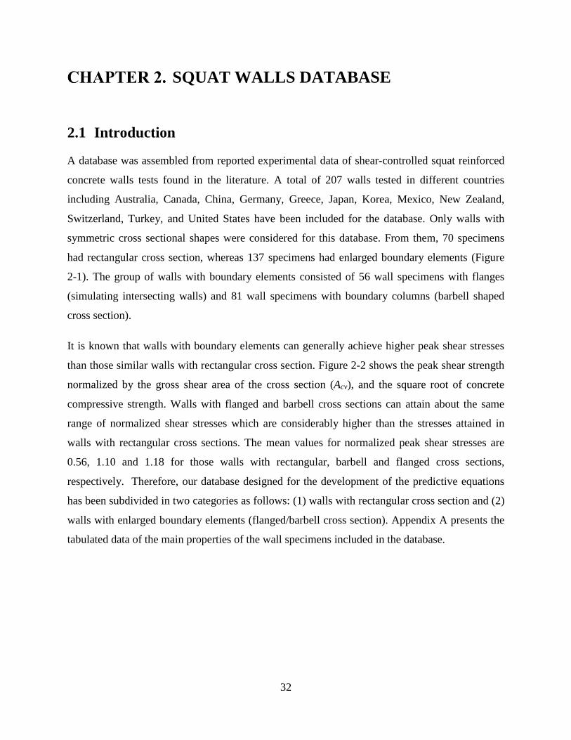
32

SQUAT WALLS DATABASE

2.1 Introduction

A database was assembled from reported experimental data of shear-controlled squat reinforced

concrete walls tests found in the literature. A total of 207 walls tested in different countries

including Australia, Canada, China, Germany, Greece, Japan, Korea, Mexico, New Zealand,

Switzerland, Turkey, and United States have been included for the database. Only walls with

symmetric cross sectional shapes were considered for this database. From them, 70 specimens

had rectangular cross section, whereas 137 specimens had enlarged boundary elements (Figure

2-1). The group of walls with boundary elements consisted of 56 wall specimens with flanges

(simulating intersecting walls) and 81 wall specimens with boundary columns (barbell shaped

cross section).

It is known that walls with boundary elements can generally achieve higher peak shear stresses

than those similar walls with rectangular cross section. Figure 2-2 shows the peak shear strength

normalized by the gross shear area of the cross section (Acv), and the square root of concrete

compressive strength. Walls with flanged and barbell cross sections can attain about the same

range of normalized shear stresses which are considerably higher than the stresses attained in

walls with rectangular cross sections. The mean values for normalized peak shear stresses are

0.56, 1.10 and 1.18 for those walls with rectangular, barbell and flanged cross sections,

respectively. Therefore, our database designed for the development of the predictive equations

has been subdivided in two categories as follows: (1) walls with rectangular cross section and (2)

walls with enlarged boundary elements (flanged/barbell cross section). Appendix A presents the

tabulated data of the main properties of the wall specimens included in the database.

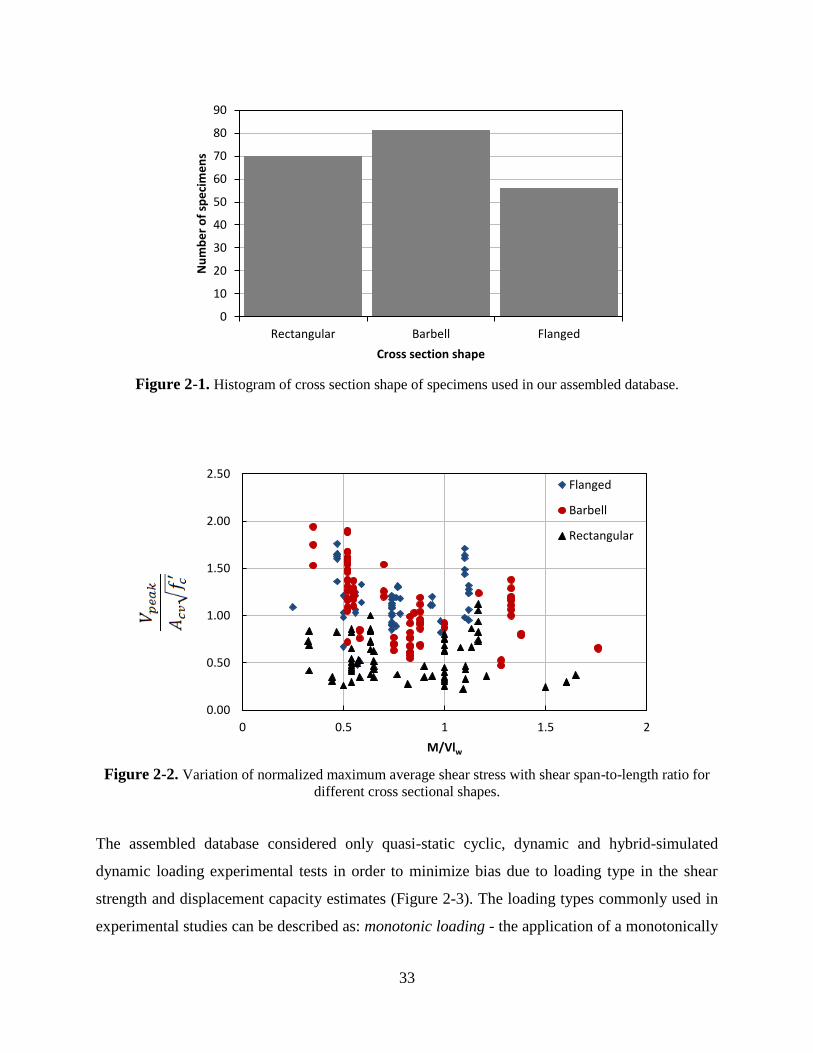
33

Figure 2-1. Histogram of cross section shape of specimens used in our assembled database.

Figure 2-2. Variation of normalized maximum average shear stress with shear span-to-length ratio for

different cross sectional shapes.

The assembled database considered only quasi-static cyclic, dynamic and hybrid-simulated

dynamic loading experimental tests in order to minimize bias due to loading type in the shear

strength and displacement capacity estimates (Figure 2-3). The loading types commonly used in

experimental studies can be described as: monotonic loading - the application of a monotonically

0

10

20

30

40

50

60

70

80

90

Rectangular Barbell Flanged

Nu

mb

er

of

spe

cim

en

s

Cross section shape

0.00

0.50

1.00

1.50

2.00

2.50

0 0.5 1 1.5 2

M/Vlw

Flanged

Barbell

Rectangular

34

increasing load in only one direction; cyclic loading - application of quasi-static lateral load

reversals with increasing force or displacement (typically two to four cycles per load step are

applied); repeated loading - similar to quasi-static cyclic loading but loaded only in one direction

(no load reversals); dynamic loading - the use of “shake tables” which simulate earthquake

loading by application of earthquake ground motion records at the foundation of the specimen;

and hybrid-simulated that consists of the simulation of earthquake ground motion loading by

application of a quasi-static lateral load (this method uses computational analysis to calculate the

corresponding lateral load at each step of the simulated input ground motion). By evaluation of

collected data, we have found that cyclic tests can yield lower shear strength than monotonically

loaded similar specimens. Since the focus of this work is on earthquake loading, tests using

monotonic or repeated loading schemes were excluded from the database as these can lead to

higher strength and considerably larger drift capacities due to the lack of cyclic cumulative

damage and/or the absence of cracking from loading in the opposite direction which may not be

representative of earthquake loading.

Figure 2-3. Histogram of loading type for the walls population included in the assembled database.

Only conventionally reinforced walls with symmetric horizontal and vertical reinforcement

arrangements, no diagonal reinforcement, and no additional dowel reinforcement at foundation

to wall interface have been considered, as commonly found in US design and construction

0

20

40

60

80

100

120

140

160

180

200

220

Cyclic Hybrid Dynamic

Nu

mb

er

of

spe

cim

en

s

Loading type

35

practice. Moderate to large scale tests, with minimum web thicknesses of 75 mm, were used here

in order to reduce bias due to small scale and material properties. Also, only walls using

conventional normalweight concrete were included in order to minimize the bias due to reduced

strength and stiffness of lightweight concrete, or due to improved tensile stress-strain behavior of

fiber-modified concrete. Only walls deemed as shear-controlled were included in the database.

Walls were considered to be shear-controlled by comparing the shear load associated with

flexural failure (Vflexure) with the peak strength (Vpeak) measured from test. A ratio of Vflexure /Vpeak

higher than one suggests that the wall is expected to have a shear-controlled failure. Walls with

aspect ratios lower than 1.5 were selected in order to further minimize the possibilities of

including flexure-controlled and mixed failure modes. Walls flexural strength was calculated by

fiber cross-section analysis using an OpenSees code (code sample can be found on Appendix D);

implementing reported steel and concrete materials properties.

OpenSees Concrete04 material (Lowes and Berry, 2009) was used as constitutive model for

concrete in the fiber cross section analyses. Conservatively, no strength increase due to

transverse steel confinement was considered and concrete tensile strength was neglected.

Reported values for the concrete parameters were used whenever possible, but when values were

not reported in the literature then the following assumptions have been made:

concrete modulus of elasticity, as per ACI 318-14 code provisions,

concrete strain at peak compressive strength, 0.002,

concrete ultimate strain, 0.004 as suggested by Mander et al. (1988).

OpenSees ReinforcingSteel material (Mohle and Kunnath, 2010) was used as the steel

constitutive model in the fiber cross section analyses. Reported values for the steel parameters

were used whenever possible, but when values were not reported in the literature then the

following assumptions have been made:

ultimate tensile strength of the steel reinforcement, 1.2fy ,

steel modulus of elasticity, 200 GPa,

steel ultimate tensile strain, 0.12,

steel strain at the onset strain hardening, 0.015,

tangent at initial strain hardening, 8275 MPa.

36

Selected wall specimens were tested in a cantilever setup with a load applied in the direction of

the plane of the wall so that the aspect ratio (hw/lw) was generally similar to M/Vlw. Note that

walls tested with restricted rotation at the top will have a hw/lw of nearly twice M/Vlw thus,

representing boundary conditions found in wall-piers which are connected to very stiff elements

at both ends. Only cantilever (fixed-free) tests were selected to eliminate bias due to boundary

conditions. Walls with openings and asymmetric cross sections were excluded from database.

Some of the walls from Carrillo and Alcocer (2013) were reinforced with non-ductile wire mesh

and were reported to fail prematurely by fracture of web reinforcement. This type of non-ductile

wire mesh reinforcement is not representative of the common US design and construction

practice and therefore, corresponding wall specimens were excluded from database. Terzioglu

tests data were reported by Opazo (2012) and Gutierrez (2012).

2.2 Walls with Rectangular Cross Section

Rectangular walls database was assembled using the results from 70 wall specimens meeting the

selection criteria found in the literature. It includes wall specimens of moderate to large scale,

built with normal and high strength concrete and steel materials. Sixty-seven of the 70 wall

specimens were tested under cyclic loading, two were tested using hybrid-simulated earthquake

loading, and one was tested using dynamic loading. Their thicknesses ranged from 76 mm to 203

mm. Aspect ratio of the walls (hw/lw) varied from 0.25 to 1.50 whereas the shear span-to-length

ratio (M/Vlw) varied from 0.33 to 1.65. About 90% of the wall specimens had aspect ratio

between 0.25 and 1.0. Length-to-thickness ratio varied from 7.5 to 54.0, but more than 95 % of

the wall specimens had a ratio below 30. Forty-two of the 70 wall specimens were tested

without axial loads, in addition to the self-weight of the specimen (wall plus top slab or top

beam). Axial load ratios were calculated as the additional applied load (P) divided by the product

of the concrete compressive strength and the gross cross sectional area (f’cAg). The remaining

walls had axial load ratios ranging from 1% to 14%. Figure 2-4 shows a summary of the

geometric properties and axial loading values for the rectangular walls used in this study. Figure

2-5 shows a summary of the reinforcement and material properties for the same population of

wall specimens.

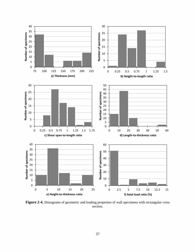
37

Figure 2-4. Histograms of geometric and loading properties of wall specimens with rectangular cross

section.

75 100 125 150 175 200 225

0

5

10

15

20

25

30

35

40

a) Thickness (mm)

Nu

mb

er

of

spe

cim

en

s

0 0.25 0.5 0.75 1 1.25 1.5

0

5

10

15

20

25

30

b) Height-to-length ratio

Nu

mb

er

of

spe

cim

en

s

0 0.25 0.5 0.75 1 1.25 1.5 1.75

0

5

10

15

20

25

30

c) Shear span-to-length ratio

Nu

mb

er

of

spe

cim

en

s

0 10 20 30 40 50 60

0

5

10

15

20

25

30

35

40

45

50

d) Length-to-thickness ratio

Nu

mb

er

of

spe

cim

en

s

0 5 10 15 20 25

0

5

10

15

20

25

30

35

40

e) Height-to-thickness ratio

Nu

mb

er

of

spe

cim

en

s

0 2.5 5 7.5 10 12.5 15

0

10

20

30

40

50

60

f) Axial load ratio (%)

Nu

mb

er

of

spe

cim

en

s

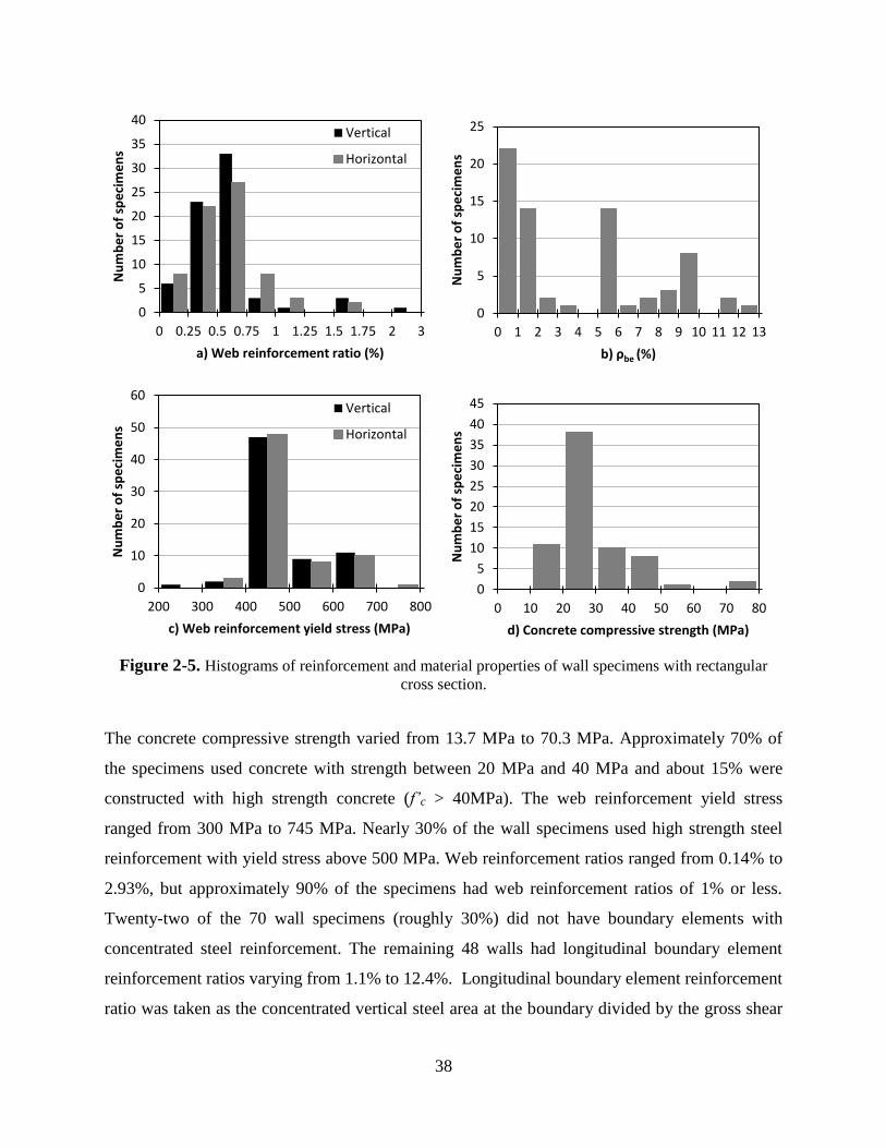
38

Figure 2-5. Histograms of reinforcement and material properties of wall specimens with rectangular

cross section.

The concrete compressive strength varied from 13.7 MPa to 70.3 MPa. Approximately 70% of

the specimens used concrete with strength between 20 MPa and 40 MPa and about 15% were

constructed with high strength concrete (f’c > 40MPa). The web reinforcement yield stress

ranged from 300 MPa to 745 MPa. Nearly 30% of the wall specimens used high strength steel

reinforcement with yield stress above 500 MPa. Web reinforcement ratios ranged from 0.14% to

2.93%, but approximately 90% of the specimens had web reinforcement ratios of 1% or less.

Twenty-two of the 70 wall specimens (roughly 30%) did not have boundary elements with

concentrated steel reinforcement. The remaining 48 walls had longitudinal boundary element

reinforcement ratios varying from 1.1% to 12.4%. Longitudinal boundary element reinforcement

ratio was taken as the concentrated vertical steel area at the boundary divided by the gross shear

0 0.25 0.5 0.75 1 1.25 1.5 1.75 2 3

0

5

10

15

20

25

30

35

40

a) Web reinforcement ratio (%)

Nu

mb

er

of

spe

cim

en

sVertical

Horizontal

0 1 2 3 4 5 6 7 8 9 10 11 12 13

0

5

10

15

20

25

b) ρbe (%)

Nu

mb

er

of

spe

cim

en

s

200 300 400 500 600 700 800

0

10

20

30

40

50

60

c) Web reinforcement yield stress (MPa)

Nu

mb

er

of

spe

cim

en

s

Vertical

Horizontal

0 10 20 30 40 50 60 70 80

0

5

10

15

20

25

30

35

40

45

d) Concrete compressive strength (MPa)

Nu

mb

er

of

spe

cim

en

s

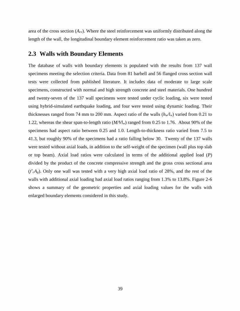
39

area of the cross section (Acv). Where the steel reinforcement was uniformly distributed along the

length of the wall, the longitudinal boundary element reinforcement ratio was taken as zero.

2.3 Walls with Boundary Elements

The database of walls with boundary elements is populated with the results from 137 wall

specimens meeting the selection criteria. Data from 81 barbell and 56 flanged cross section wall

tests were collected from published literature. It includes data of moderate to large scale

specimens, constructed with normal and high strength concrete and steel materials. One hundred

and twenty-seven of the 137 wall specimens were tested under cyclic loading, six were tested

using hybrid-simulated earthquake loading, and four were tested using dynamic loading. Their

thicknesses ranged from 74 mm to 200 mm. Aspect ratio of the walls (hw/lw) varied from 0.21 to

1.22, whereas the shear span-to-length ratio (M/Vlw) ranged from 0.25 to 1.76. About 90% of the

specimens had aspect ratio between 0.25 and 1.0. Length-to-thickness ratio varied from 7.5 to

41.3, but roughly 90% of the specimens had a ratio falling below 30. Twenty of the 137 walls

were tested without axial loads, in addition to the self-weight of the specimen (wall plus top slab

or top beam). Axial load ratios were calculated in terms of the additional applied load (P)

divided by the product of the concrete compressive strength and the gross cross sectional area

(f’cAg). Only one wall was tested with a very high axial load ratio of 28%, and the rest of the

walls with additional axial loading had axial load ratios ranging from 1.3% to 13.8%. Figure 2-6

shows a summary of the geometric properties and axial loading values for the walls with

enlarged boundary elements considered in this study.

40

Figure 2-6. Histograms of geometric and loading properties of walls with flanged and barbell cross

section.

The concrete compressive strength varied from 17.4 MPa to 103.4 MPa. Approximately 70% of

wall specimens used concrete with strength between 20 MPa and 40 MPa, and about 25% of

50 75 100 125 150 175 200

0

20

40

60

80

100

120

a) Thickness (mm)

Nu

mb

er

of

spe

cim

en

s

0 0.25 0.5 0.75 1 1.25 1.5

0

10

20

30

40

50

60

b) Height -to-length ratio

Nu

mb

er

of

spe

cim

en

s

0 0.25 0.5 0.75 1 1.25 1.5 1.75 2

0

10

20

30

40

50

60

70

c) Shear span-to-length ratio

Nu

mb

er

of

spe

cim

en

s

0 10 20 30 40 50

0

10

20

30

40

50

60

70

80

d) Length-to-thickness ratio

Nu

mb

er

of

spe

cim

en

s

0 5 10 15 20 25 30 35

0

10

20

30

40

50

60

70

e) Height-to-thickness ratio

Nu

mb

er

of

spe

cim

en

s

0 5 10 15 20 25 30

0

10

20

30

40

50

60

70

f) Axial load ratio (%)

Nu

mb

er

of

spe

cim

en

s

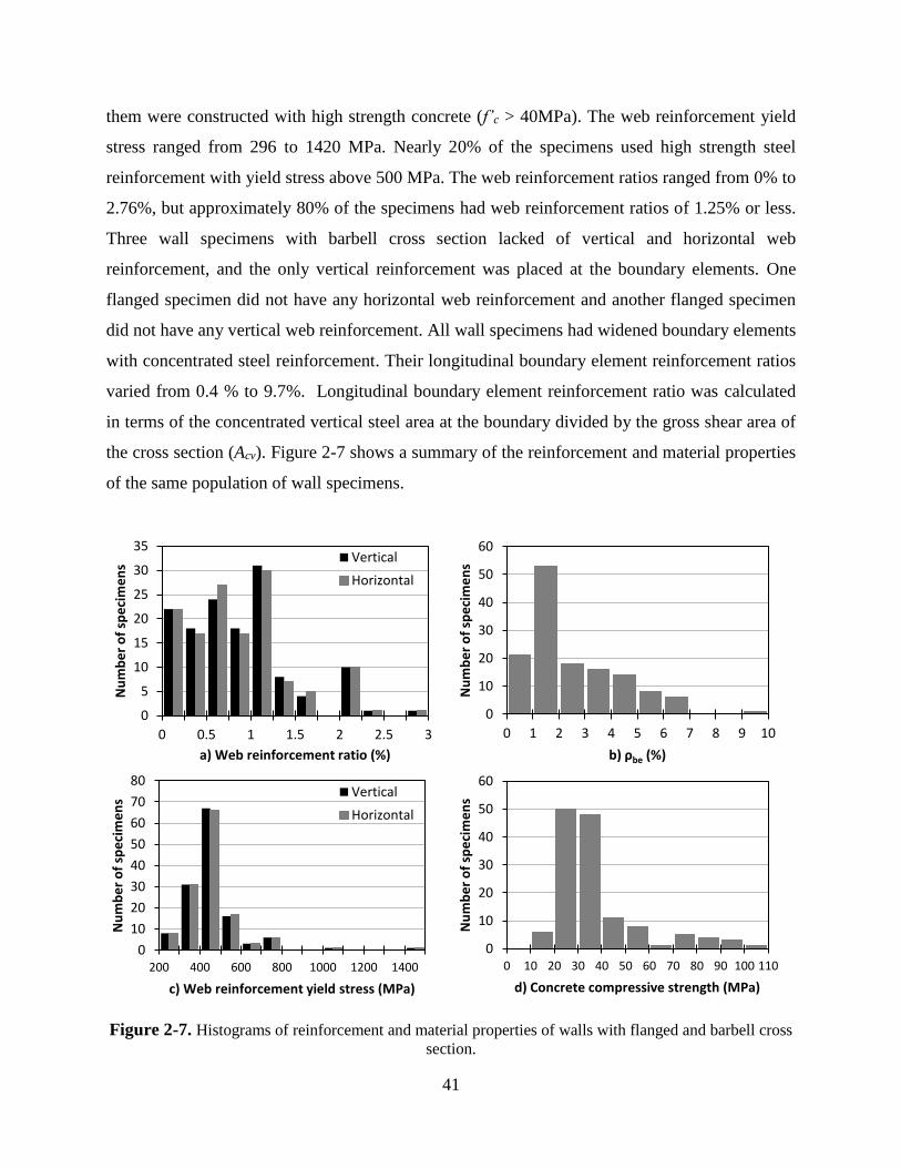
41

them were constructed with high strength concrete (f’c > 40MPa). The web reinforcement yield

stress ranged from 296 to 1420 MPa. Nearly 20% of the specimens used high strength steel

reinforcement with yield stress above 500 MPa. The web reinforcement ratios ranged from 0% to

2.76%, but approximately 80% of the specimens had web reinforcement ratios of 1.25% or less.

Three wall specimens with barbell cross section lacked of vertical and horizontal web

reinforcement, and the only vertical reinforcement was placed at the boundary elements. One

flanged specimen did not have any horizontal web reinforcement and another flanged specimen

did not have any vertical web reinforcement. All wall specimens had widened boundary elements

with concentrated steel reinforcement. Their longitudinal boundary element reinforcement ratios

varied from 0.4 % to 9.7%. Longitudinal boundary element reinforcement ratio was calculated

in terms of the concentrated vertical steel area at the boundary divided by the gross shear area of

the cross section (Acv). Figure 2-7 shows a summary of the reinforcement and material properties

of the same population of wall specimens.

Figure 2-7. Histograms of reinforcement and material properties of walls with flanged and barbell cross

section.

0 0.5 1 1.5 2 2.5 3

0

5

10

15

20

25

30

35

a) Web reinforcement ratio (%)

Nu

mb

er

of

spe

cim

en

s

Vertical

Horizontal

0 1 2 3 4 5 6 7 8 9 10

0

10

20

30

40

50

60

b) ρbe (%)

Nu

mb

er

of

spe

cim

en

s

200 400 600 800 1000 1200 1400

0

10

20

30

40

50

60

70

80

c) Web reinforcement yield stress (MPa)

Nu

mb

er

of

spe

cim

en

s

Vertical

Horizontal

0 10 20 30 40 50 60 70 80 90 100 110

0

10

20

30

40

50

60

d) Concrete compressive strength (MPa)

Nu

mb

er

of

spe

cim

en

s

42

SHEAR STRENGTH OF SQUAT WALLS

WITH RECTANGULAR CROSS SECTION

3.1 Introduction

Statistical analyses have been carried out from the assembled database, as described in Chapter

2. As previously noted, wall specimens with enlarged boundary elements (i.e. barbell and

flanged cross section) generally achieved higher shear strength than comparable specimens with

rectangular cross section. Therefore, the assessment of available predictive equations and

development of new predictive equations were addressed separately for both groups of walls.

The discussion on the strength of walls with boundary elements is presented in Chapter 5.

It has been found that the commonly used equations, as described in US standards and literature,

vary significantly in functional form as well as in predictive performance. Even when the

behavior of squat walls is significantly different from walls with higher aspect ratios, these

equations have been generated based on experimental data, including walls of different

characteristics which do not necessarily focus on squat walls. Also, some of the commonly used

equations do not differentiate between walls with rectangular or barbell cross section.

Many equations were found in current US design codes (ACI 318, ACI 349, ASCE 43-05) and in

literature (e.g., Barda et al., 1977; Wood et al., 1990) for the prediction of the peak shear strength

of reinforced concrete walls. However, comparison against experimental results show that these

equations yield significantly scattered strength predictions for squat walls. Some reasons for their

scattered predictions originate from the limited data on which the expressions are based. For

example, ACI 318-14 equations are mostly based on data from moderate aspect ratio walls, and

were modified by either imposing limits of reinforcement and/or incorporating a factor to include

the strength characteristics of low aspect ratio walls (Cardenas et al., 1973). ASCE 43 equation is

based on Barda’s experiments (Barda, 1972; Barda et al., 1977) and was modified to provide a

lower-bound solution when compared with some experiments available at that time. It is

important to note that the US code equations have remained basically unchanged for over 30

years, while significant new experimental data is now available. Extensive research has been

43

performed during the past few years (e.g., Carrillo et al., 2013; Gulec and Whittaker 2009;

Massone, 2010a; etc.) to address this situation, however the development of better equations to

assess the peak shear strength of squat RC walls is still necessary, since the lateral strength and

performance of these walls relies mostly on its shear strength.

This chapter presents an evaluation of current expressions for the prediction of peak shear

strength of squat reinforced concrete walls with rectangular cross section available in US design

codes and in literature. The performance of each of the selected equations is assessed by

comparing the strength predictions with experimental strength from the assembled database for

walls with rectangular cross section. The experimental peak shear strength of each wall was

taken as the average of the peak strengths measured from the first and third quadrants (i.e.

positive and negative loading directions, respectively). Key parameters influencing the peak

shear strength were identified and a new equation to predict the peak shear strength of squat

walls with rectangular cross sections is presented. The new equation was obtained from

multivariable regression analyses using an assembled experimental database and aims to improve

current peak shear estimates. The new expression presented herein is intended to be used in the

design and assessment of structures with RC squat walls.

3.2 Current Expressions for Peak Shear Strength

The following subsections discuss the selected current equations for shear strength prediction.

The equations shown are similar to those found on the corresponding references, but the names

and subscripts for parameters have been modified to maintain uniformity within equations,

database and manuscript. Also, the equations are expressed in terms of nominal loads and

nominal strength (without applying any strength reduction factor) for the purpose of comparison.

3.2.1 ACI 318-14

The ACI 349-13 Code Requirements for Nuclear Safety Related Concrete Structures uses all the

same provisions of the ACI 318-14 for evaluating peak shear strength of walls, with the

difference that provisions for lightweight aggregates (i.e., λ factor) were omitted from the entire

code and commentary, since the structural configuration and structural member sizing is

typically controlled by live loads, seismic loads or shielding requirements, and not floor dead

44

loads. Section R21.2.4 of the ACI 349-13 commentary states that lightweight concrete is not

permitted in nuclear safety-related structures.

The ACI 318-14 has two different sets of provisions for evaluating the peak shear strength of

reinforced concrete walls. The first set, given in section 11.5 of the code, is intended to be used

for shear walls with general loading. The second set, specified in section 18.10, is intended to be

used specifically for special structural walls of earthquake resistant structures.

For design purposes, the strength shall be calculated by multiplying the nominal strength by the

strength reduction factor (φ). This factor is determined according to section 9.3 of the code and is

equal to 0.75 for most cases of shear and torsion. The code requires that, for any structural

member designed to resist earthquake effects, the strength reduction factor (φ) shall be 0.60 if its

nominal shear strength is less than the shear corresponding to the development of the nominal

flexural strength of the member. This is commonly applicable to squat walls and other structural

members with low shear span-to-length ratio (M/Vlw), where the necessary reinforcement to

provide shear strength in excess of the corresponding shear at flexural strength becomes

impractical.

3.2.1.1 Chapter 11 of ACI 318-14

The provisions first appeared in Chapter 11 of ACI 318-71 and have remained unchanged since

then. The wall nominal shear strength loaded in the direction of the plane of the wall is

calculated using equation 3-1, which attributes part of the strength to the concrete and the rest to

the web reinforcement as it has been typically used in the US design practice for many reinforced

concrete members. Although research show that higher shear stresses can be obtained in some

types of walls, an upper limit of 0.83√𝑓𝑐′ is conservatively imposed in the nominal shear stress

to preclude diagonal compression failure and to limit the redistribution of shear force.

dtfVVV wcscn

'83.0

(3-1)

where Vn is the nominal shear strength (N); f’c is the uniaxial compressive strength of concrete

(MPa); tw is the wall web thickness (mm); d is the effective depth of the cross section (mm) and

45

is taken as 80% of the length of wall (0.8lw) or determined by strain compatibility analysis; Vc is

the nominal shear strength carried by concrete (N); and Vs is the shear strength carried by steel

reinforcement (N).

The nominal shear strength provided by concrete is taken as the lesser of the values obtained by

equations 3-2 and 3-3. When the term (𝑀𝑢 𝑉𝑢⁄ − 𝑙𝑤 2)⁄ is negative equation 3-3 shall not apply.

The nominal shear strength provided by horizontal reinforcement can be calculated using

equation 3-4.

w

wccl

PddtfV

427.0 '

(3-2)

dtl

V

M

tl

Pfl

fV ww

ww

cw

cc

2

2.01.0

05.0

'

'

(3-3)

s

dfAV

yv

s

(3-4)

where P is the total applied axial load normal to the cross section (N); M is the flexural moment

at section (N•mm); V is the shear loading at section (N); Av is the area of shear reinforcement

(mm2) within spacing s; s is center-to-center spacing of horizontal reinforcement (mm); fy is the

yield stress of the shear reinforcement (MPa); and λ is the modification factor reflecting the

reduced mechanical properties of lightweight concrete (1.0 for normalweight concrete, 0.85 for

sand-lightweight concrete and 0.75 for all-lightweight concrete).

As reported by Cardenas et al. (1973), ACI 318 assumes that shear strength provided by concrete

corresponds to shear force that would produce significant inclined cracking. Inclined cracks are

generally classified as either “web-shear” or “flexure-shear”. Web shear cracks are those that

form near the neutral axis of the cross section and propagate inclined to the member axis before

any flexural cracking has occurred in their vicinity. On the other hand, flexure-shear cracks begin

with a flexural crack at the extreme tension fiber and, as a result of the applied shear, becomes

inclined in the direction of increasing moment as it propagates through the cross section.

46

Equation 3-2 has been derived based upon the assumption that the development of inclined or

“web-shear” cracking of a wall with combined axial and shear loading will occurs when the

maximum principal tensile stress in an interior point of the cross section reaches a value

of 0.33√𝑓𝑐′. Equation 3-3 predicts flexure-shear cracking strength as the shear that produces

flexural cracking stress of 0.5√𝑓𝑐′ at a section located lw/2 above the section being investigated,

plus the shear required to transform the incipient flexural crack into an inclined and fully

developed flexure-shear crack (conservatively taken as 0.05√𝑓𝑐′ ). According to section 11.5.4.7

of the ACI 318-14, the critical section for design in the lower portions of the wall can be taken at

a distance of the lesser of lw/2 and hw/2 from the base.

Sections 11.6 and 11.7 also establish limits on the quantity and spacing of reinforcement as

follows:

Spacing for horizontal reinforcement shall not exceed the smallest of lw/5, 3tw and 450

mm.

Spacing of vertical reinforcement shall not exceed the smallest of lw/3, 3tw and 450 mm.

The ratio of vertical reinforcement (ρv) shall not be smaller than 0.0025 and the

calculated by equation 3-5. The value calculated with equation 3-5 need not be larger

than the required to meet the design strength (φVn ≥ Vu).

Where Vu ≥ 0.5 φVc, the horizontal (transverse) reinforcement ratio shall be at least

0.0025 and the vertical (longitudinal) reinforcement ratio shall be the greater of 0.0025

and the value calculated with the following equation as established in code section 11.6.2.

𝜌𝑣 = 0.0025 + 0.5 (2.5 −ℎ𝑤

𝑙𝑤) (𝜌ℎ − 0.0025) (3-5)

Where Vu < 0.5 φVc, more relaxed reinforcement limits are allowed as per section 11.6.1.

As stated by Barda et al. (1977), horizontal reinforcement becomes less effective than vertical

reinforcement for shear strength in low rise walls. Their findings also suggests that for walls with

aspect ratios lower than 0.5 the shear strength was almost insensitive to the horizontal

reinforcement ratio, but was effective to produce more distributed crack patterns with reduced

crack widths, which enhances energy dissipation. In a similar manner, for walls with higher

aspect ratios (hw/lw ≥ 1.0), vertical reinforcement is less effective for shear strength, but promotes

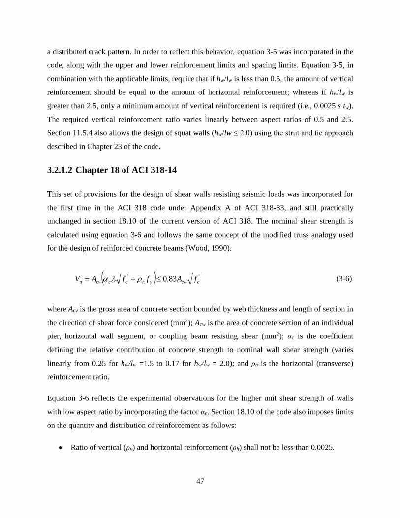
47

a distributed crack pattern. In order to reflect this behavior, equation 3-5 was incorporated in the

code, along with the upper and lower reinforcement limits and spacing limits. Equation 3-5, in

combination with the applicable limits, require that if hw/lw is less than 0.5, the amount of vertical

reinforcement should be equal to the amount of horizontal reinforcement; whereas if hw/lw is

greater than 2.5, only a minimum amount of vertical reinforcement is required (i.e., 0.0025 s tw).

The required vertical reinforcement ratio varies linearly between aspect ratios of 0.5 and 2.5.

Section 11.5.4 also allows the design of squat walls (hw/lw ≤ 2.0) using the strut and tie approach

described in Chapter 23 of the code.

3.2.1.2 Chapter 18 of ACI 318-14

This set of provisions for the design of shear walls resisting seismic loads was incorporated for

the first time in the ACI 318 code under Appendix A of ACI 318-83, and still practically

unchanged in section 18.10 of the current version of ACI 318. The nominal shear strength is

calculated using equation 3-6 and follows the same concept of the modified truss analogy used

for the design of reinforced concrete beams (Wood, 1990).

'' 83.0 ccwyhcccvn fAffAV (3-6)

where Acv is the gross area of concrete section bounded by web thickness and length of section in

the direction of shear force considered (mm2); Acw is the area of concrete section of an individual

pier, horizontal wall segment, or coupling beam resisting shear (mm2); αc is the coefficient

defining the relative contribution of concrete strength to nominal wall shear strength (varies

linearly from 0.25 for hw/lw =1.5 to 0.17 for hw/lw = 2.0); and ρh is the horizontal (transverse)

reinforcement ratio.

Equation 3-6 reflects the experimental observations for the higher unit shear strength of walls

with low aspect ratio by incorporating the factor αc. Section 18.10 of the code also imposes limits

on the quantity and distribution of reinforcement as follows:

Ratio of vertical (ρv) and horizontal reinforcement (ρh) shall not be less than 0.0025.

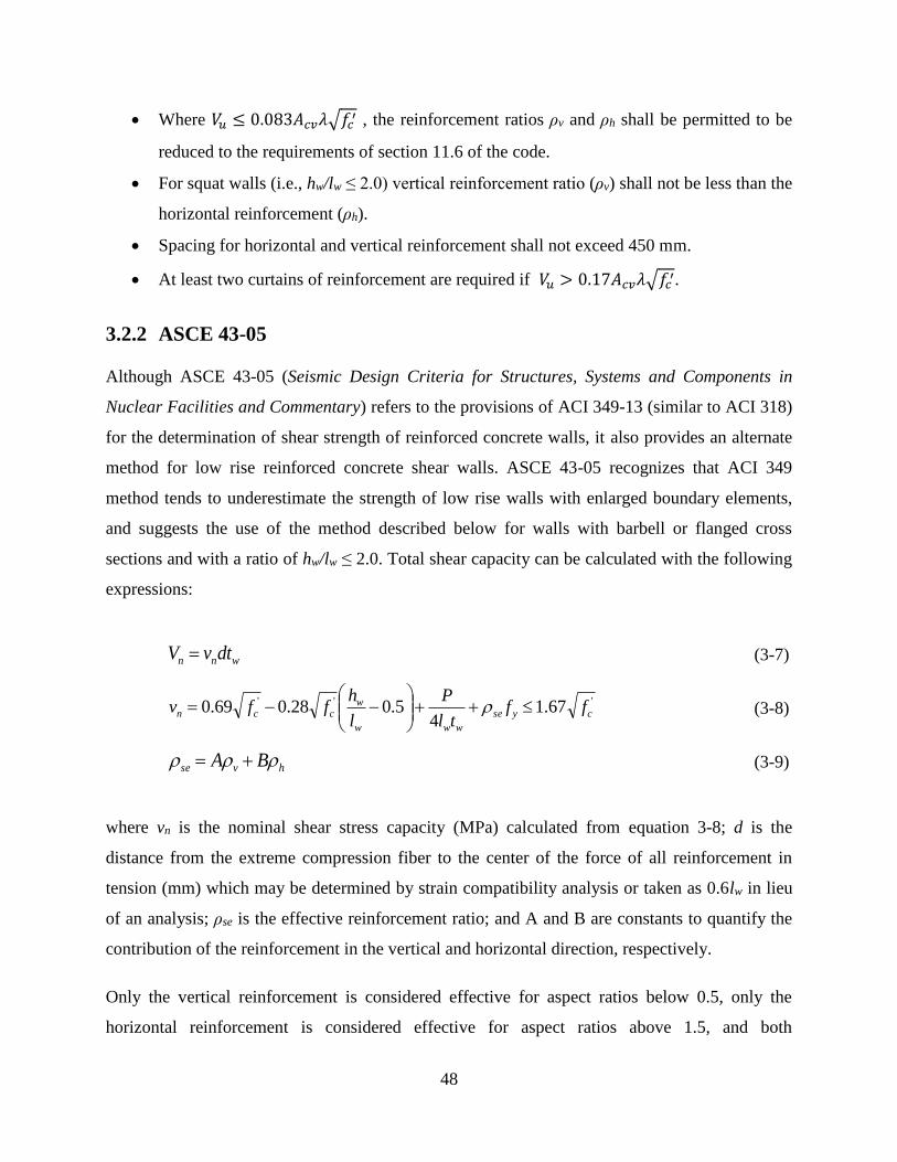
48

Where 𝑉𝑢 ≤ 0.083𝐴𝑐𝑣𝜆√𝑓𝑐′ , the reinforcement ratios ρv and ρh shall be permitted to be

reduced to the requirements of section 11.6 of the code.

For squat walls (i.e., hw/lw ≤ 2.0) vertical reinforcement ratio (ρv) shall not be less than the

horizontal reinforcement (ρh).

Spacing for horizontal and vertical reinforcement shall not exceed 450 mm.

At least two curtains of reinforcement are required if 𝑉𝑢 > 0.17𝐴𝑐𝑣𝜆√𝑓𝑐′.

3.2.2 ASCE 43-05

Although ASCE 43-05 (Seismic Design Criteria for Structures, Systems and Components in

Nuclear Facilities and Commentary) refers to the provisions of ACI 349-13 (similar to ACI 318)

for the determination of shear strength of reinforced concrete walls, it also provides an alternate

method for low rise reinforced concrete shear walls. ASCE 43-05 recognizes that ACI 349

method tends to underestimate the strength of low rise walls with enlarged boundary elements,

and suggests the use of the method described below for walls with barbell or flanged cross

sections and with a ratio of hw/lw ≤ 2.0. Total shear capacity can be calculated with the following

expressions:

wnn dtvV

(3-7)

''' 67.1

45.028.069.0 cyse

www

wccn ff

tl

P

l

hffv

(3-8)

hvse BA

(3-9)

where vn is the nominal shear stress capacity (MPa) calculated from equation 3-8; d is the

distance from the extreme compression fiber to the center of the force of all reinforcement in

tension (mm) which may be determined by strain compatibility analysis or taken as 0.6lw in lieu

of an analysis; ρse is the effective reinforcement ratio; and A and B are constants to quantify the

contribution of the reinforcement in the vertical and horizontal direction, respectively.

Only the vertical reinforcement is considered effective for aspect ratios below 0.5, only the

horizontal reinforcement is considered effective for aspect ratios above 1.5, and both

49

reinforcement contributions vary linearly for aspect ratios between 0.5 and 1.5. Constants A and

B are calculated as follows based on the aspect ratio hw/lw:

if hw/lw ≤ 0.5 A = 1 B = 0

if 0.5 < hw/lw < 1.5 A = - hw/lw + 1.5 B = hw/lw – 0.5

if hw/lw ≥ 1.5 A = 0 B = 1

According to ASCE 43-05, equation 3-8 is applicable to shear walls with reinforcement ratios (ρv

and ρh) less than or equal to 0.01. When ρv or ρh exceeds 0.01, the effective reinforcement ratio

(ρse) shall be limited to 0.01 in the calculation of strength. The ASCE 43 method is based on the

equations proposed by Barda (Barda, 1972; Barda et al., 1977) and was modified to account for

both horizontal and vertical steel, and provide a lower-bound solution when compared with some

experiments available at that time.

3.2.3 Barda et al. (1977)

Eight RC squat wall specimens with heavily reinforced and well-confined flanges (end walls)

were tested in under lateral load and without axial load. Their study involved six walls with

cyclic loading, two walls with monotonic loading and one wall that was repaired and retested

after attaining heavy damage. The shear span-to-length ratios of the test specimens varied from

0.25 to 1.0. They calibrated equation 3-10 to give a close prediction of the shear strength of the

tested wall specimens. However, they proposed equation 3-11 for design purposes to include the

effect of axial load.

dtfl

hffV wyv

w

w

ccn

2

128.069.0 '' (3-10)

dtf

tl

P

l

hffV wyv

www

wccn

421.067.0 ''

(3-11)

Equations 3-10 and 3-11 include only the vertical reinforcement ratio since the authors observed

that the horizontal reinforcement did not show significant contribution to shear strength on the

tested specimens with lower aspect ratios. However, they noted that horizontal reinforcement had

50

a considerable effect in generating more evenly distributed, closely spaced, and narrow width

crack pattern that enhanced hysteretic behavior and post peak strength. Therefore, they

recommended providing equal reinforcement ratio in both, vertical and horizontal directions.

Also, based on the characteristics of the wall specimens tested in their experimental program, the

authors suggested that the equations were applicable for aspect ratios equal or less than one; and

reinforcement ratios ranging from 0.0025 to 0.005 and somewhat higher. For the calculations

presented herein, d was assumed as 0.6lw.

3.2.4 Wood (1990)

Wood (1990) evaluated the results of 143 low-rise wall specimens which included rectangular,

flanged and barbell cross sections. Wood proposed the equation 3-12 to estimate the shear

strength of squat RC walls:

'' 83.04

5.0 ccv

yvf

ncvc fAfA

VAf (3-12)

where, Avf is the total vertical reinforcement area in the wall (mm2).

Wood observed that the maximum average shear stress tended to increase with an increase in the

amount of vertical reinforcement in both web and boundary elements. The author proposed a

semi-empirical expression (Equation 3-12), derived by using a shear-friction analogy, and

calibrated against experimental data of squat RC walls tests collected from literature. The author

found that lower bounds for the strength of the walls considered were well represented by

0.5𝐴𝑐𝑣√𝑓𝑐′ and 𝐴𝑣𝑓𝑓𝑦 4⁄ but also established an upper limit of 0.83𝐴𝑐𝑣√𝑓𝑐

′ to avoid failure

modes associated with compressive strength of concrete.

3.3 Development of New Peak Shear Strength Predictive Equation

A statistical approach was used to develop and calibrate an equation that improves the actual

estimates of peak shear strength of squat RC walls with rectangular cross section. Multivariable

linear regression analyses were performed to produce an empirical equation that better fits the

included database of 70 squat RC walls with rectangular cross section. The goal was to lower the

51

standard deviation and coefficient of variation of the predicted-to-measured shear strength ratio.

The goal was also to obtain a mean predicted-to-measured strength ratio near to 1.0, while

keeping the percentage of over-predictions around 50% which means that the predicted strength

would be, on average, nearer to the experimental strength. Experimental peak strength was taken

as the average of the peak strengths recorded in the positive (first quadrant of hysteresis) and

negative (third quadrant of hysteresis) loading directions.

A functional equation form was selected based on Barda’s proposed expressions and based on

common ACI seismic design expressions. The parameters found on these equations are in

general agreement with the parameters having important influence on shear strength as reported

by several researchers. Additional predictive parameters were identified by reviewing the

findings from numerous experimental programs and extended to account for the vertical,

horizontal and boundary element reinforcement. To arrive to the final parameter selection,

multivariable linear regression analysis was run using several different combinations of the

previously identified parameters to generate a calibrated equation on each run. Finally, the

calibrated equation with the parameter combination that yields less variability when compared to

the assembled database was selected. The following set of expressions includes the parameters

that were found to be better correlated to the experimental strength and is calibrated to best fit

the data within the database:

cvybebeysese

gw

w

ccn AffA

P

l

hffV

39.047.041.0080.0068.035.0 '' (3-13)

yhyvyse BfAff (3-14)

hvse BA (3-15)

cv

sbebe A

A

(3-16)

where ρbe is the longitudinal boundary element reinforcement ratio; Asbe is the longitudinal

boundary reinforcement area (mm2); and constants A and B are calculated as follows depending

on the aspect ratio hw/lw:

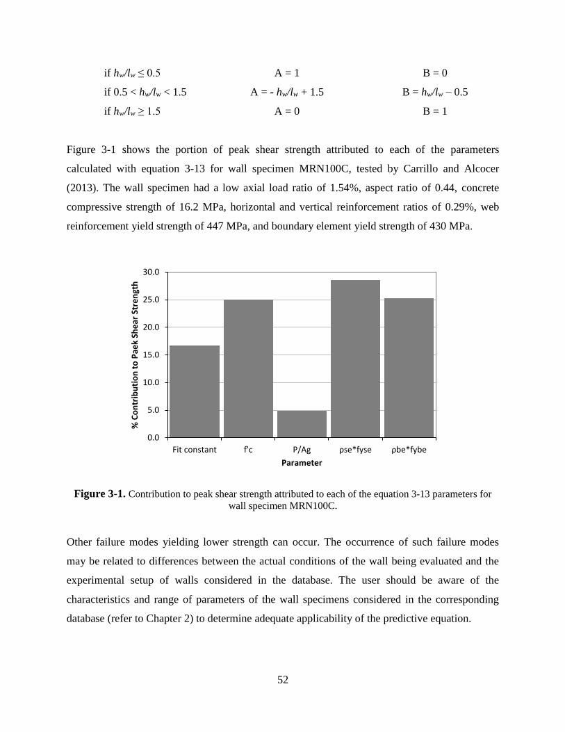
52

if hw/lw ≤ 0.5 A = 1 B = 0


if hw/lw ≥ 1.5 A = 0 B = 1

Figure 3-1 shows the portion of peak shear strength attributed to each of the parameters

calculated with equation 3-13 for wall specimen MRN100C, tested by Carrillo and Alcocer

(2013). The wall specimen had a low axial load ratio of 1.54%, aspect ratio of 0.44, concrete

compressive strength of 16.2 MPa, horizontal and vertical reinforcement ratios of 0.29%, web

reinforcement yield strength of 447 MPa, and boundary element yield strength of 430 MPa.

Figure 3-1. Contribution to peak shear strength attributed to each of the equation 3-13 parameters for

wall specimen MRN100C.

Other failure modes yielding lower strength can occur. The occurrence of such failure modes

may be related to differences between the actual conditions of the wall being evaluated and the

experimental setup of walls considered in the database. The user should be aware of the

characteristics and range of parameters of the wall specimens considered in the corresponding

database (refer to Chapter 2) to determine adequate applicability of the predictive equation.

0.0

5.0

10.0

15.0

20.0

25.0

30.0

Fit constant f'c P/Ag ρse*fyse ρbe*fybe

% C

on

trib

uti

on

to

Pae

k Sh

ear

Str

en

gth

Parameter

53

Some disagreement among research findings and common equations in terms of the effectiveness

of the vertical and horizontal reinforcement to provide shear strength was found. The majority of

researchers (e.g., Barda, 1977; Greifenhagen and Lestuzzi, 2005, etc.) agree in the fact that

horizontal reinforcement contribution to shear strength is marginal while vertical reinforcement

has significant effect on shear strength in walls with very low aspect ratios (e.g., 0.5 or less).

However, the results of walls with aspect ratios around 1.0 show some inconsistency in terms of

the effectiveness of vertical and horizontal reinforcements (Cardenas et al., 1980; Maier, 1991;

Dabbagh, 2005; Luna et al., 2015; etc.). For walls with aspect ratios around 1.0, some

researchers found both reinforcements to be effective in contributing to peak shear strength while

others reported that horizontal reinforcement did not contribute significantly to the shear

strength. However, those researchers who found horizontal reinforcement not very effective in

providing shear strength, reported that horizontal reinforcement was more influent on improving

crack distribution, energy dissipation and post-peak response. On the other hand, the

effectiveness of horizontal reinforcement in providing shear strength on slender walls (e.g.,

aspect ratios of 2.0 or higher) has been well established in literature.

In general, it appears that the shear strength of walls with very low aspect ratios tend to be more

influenced by the vertical reinforcement; and the horizontal reinforcement helps on improving

the hysteretic behavior, energy dissipation and maintaining the strength at higher drift levels.

However, the role of vertical and horizontal reinforcements seems to gradually invert as the

aspect ratio increases. To address this issue ASCE 43-05 standard implements an effective

reinforcement ratio, which varies the effectiveness of the vertical and horizontal reinforcement

ratios as a function of the wall aspect ratio (Figure 3-2). ACI 318-14 and ACI 349-13 do not

directly consider the vertical reinforcement contribution but require vertical reinforcement ratio

to be at least equal to the calculated horizontal reinforcement ratio for squat walls with aspect

ratios equal or less than 2.0 to assure adequate steel reinforcement.

In order to identify which parameter produced a better prediction, the parameter associated with

the strength provided by the reinforcement was evaluated by one-at-a-time parameter variation.

The use of vertical distributed reinforcement only, total vertical reinforcement (including

boundary element reinforcement) only, horizontal reinforcement only, both horizontal and

vertical distributed reinforcements in separate terms and an effective reinforcement ratio that

54

combines both distributed reinforcements in one term (in the same fashion as in ASCE 43-05)

were considered. The last resulted to be a better predictive parameter for steel contribution to

shear strength as it produced the least variability. Using the effective reinforcement ratio to

consider the contribution of both steel reinforcements as a function of aspect ratio (Figure 3-2)

seems to be a reasonable assumption and is in good general agreement with experimental

findings.

Figure 3-2. Variation of effective reinforcement constants with aspect ratio.

It has been consistently reported by researchers that walls with lower aspect ratios or lower shear

span-to-length ratios can yield higher shear stress capacities. This has been commonly attributed

to an increase in the shear carried by concrete as the aspect ratio decreases. In a preliminary

study, the aspect ratio was treated as a separate term and compared to equation calibration using

a term that considers the product of a concrete strength parameter and the aspect ratio. It was

found that using the product of aspect ratio and a concrete strength parameter produced better

predictions than using the aspect ratio separately. Additional to the term considering the product

of aspect ratio and concrete strength, the use of another term with concrete strength parameter

only was also considered, which further improved the predictions. Different combinations using

the aspect ratio and the shear span-to-length ratio were evaluated. Also, the use of the square root

-0.2

0.0

0.2

0.4

0.6

0.8

1.0

1.2

0 0.5 1 1.5 2

Co

nst

ants

A a

nd

B

hw/lw

A

B

55

of the concrete compressive strength (√𝑓𝑐′) versus using the compressive strength itself (f’c) was

considered.

The aspect ratio (hw/lw) was found to produce better correlation with the included database (with

cantilever test setup) than the shear span (M/Vlw). The aspect ratio is a more practical parameter

for design purposes, since it does not depend on structural analysis to calculate values for

moment and shear. However, if a wall pier with both ends fixed is being considered, then the use

of the M/Vlw would be more appropriate. The concrete compressive strength (f’c) resulted to be a

better strength prediction parameter; with best results when a concrete strength term and another

term with the product of concrete strength and wall aspect ratio were included in the equation.

The boundary element reinforcement ratio is not considered in most equations. However, several

researchers (e.g., Endo, 1980; Wood, 1990; and Terzioğlu, 2011) have found that the boundary

element reinforcement affects both the shear load transfer mechanism and the peak shear

strength even in shear-dominated walls with very low aspect ratios. Therefore, a term with the

longitudinal boundary element reinforcement ratio (ρbe), calculated as the ratio of longitudinal

boundary reinforcement area in tension to the effective shear area (Asbe/Acv), was included

resulting in an enhancement in the predictive performance of the equation. Another option where

the ρbe was calculated as the ratio of longitudinal boundary reinforcement area in tension to the

gross area of the corresponding boundary element (Asbe/Abe) was evaluated as well, but better

predictions were obtained using (Asbe/Acv).

It has also been widely recognized that axial loads can enhance the shear load carrying capacity

of reinforced concrete walls of higher aspect ratios. The same behavior was observed from

different researchers for squat RC walls. Therefore, the axial load ratio (P/Ag) was incorporated

in the equation form. The increase in shear strength due to axial loads may be attributed to two

major mechanisms. First, the axial force enhances the frictional force transfer through cracks and

construction joints. Secondly, the change in the biaxial stress state of the concrete panel can

increase concrete shear strength. Results from several researchers (e.g., Salonikios et al., 1999;

Palermo and Vecchio, 2002; Greifenhagen and Lestuzzi, 2005; Xiang, 2009; etc.) suggest that

low axial load ratios in the order of 5% are enough to effectively reduce the base sliding

56

displacements (in walls with construction joints), and thus help prevent premature sliding failure

of squat RC walls.

3.4 Evaluation of Selected Peak Shear Strength Equations

In this section the selected commonly used predictive equations and the new expression

developed herein (presented in last section) will be evaluated in terms of their predictive

performance by using a statistical approach and comparing to the experimental results compiled

in the assembled database. In order to eliminate bias due to load amplification factors and

resistance reduction factors between codes, the equations are modified to use nominal loads and

nominal strengths. Also, the calculated peak and nominal shear strengths (Vpeak and Vn) were then

normalized with the effective shear area of the section (Acv) to eliminate the test scale differences

between different experimental programs, so that all the parameters were worked in terms of

stress instead of force. The normalization of the shear force with Acv also allows for a fair

comparison between the available equations and the developed equation since different effective

depth (d) definitions are suggested among the available expressions.

In order to evaluate the suitability of the proposed equation, it is compared against several

widely-used equations in terms of the predicted-to-measured strength ratio. Figure 3-3 shows a

graphic representation of the correlation of the calculated shear stress capacity vs the measured

peak shear stress for the 70 rectangular cross section wall tests in the database, and for each of

the equations discussed on section 3.2.

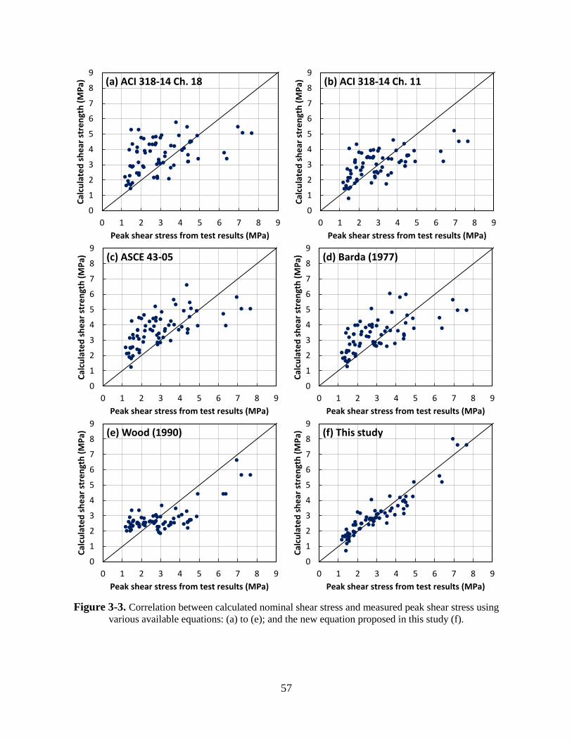
57

Figure 3-3. Correlation between calculated nominal shear stress and measured peak shear stress using

various available equations: (a) to (e); and the new equation proposed in this study (f).

0

1

2

3

4

5

6

7

8

9

0 1 2 3 4 5 6 7 8 9

Cal

cula

ted

sh

ear

str

en

gth

(M

Pa)

Peak shear stress from test results (MPa)

(a) ACI 318-14 Ch. 18

0

1

2

3

4

5

6

7

8

9

0 1 2 3 4 5 6 7 8 9

Cal

cula

ted

sh

ear

str

en

gth

(M

Pa)


(b) ACI 318-14 Ch. 11

0

1

2

3

4

5

6

7

8

9

0 1 2 3 4 5 6 7 8 9

Cal

cula

ted

sh

ear

str

en

gth

(M

Pa)


(c) ASCE 43-05

0

1

2

3

4

5

6

7

8

9

0 1 2 3 4 5 6 7 8 9

Cal

cula

ted

sh

ear

str

en

gth

(M

Pa)


(d) Barda (1977)

0

1

2

3

4

5

6

7

8

9

0 1 2 3 4 5 6 7 8 9

Cal

cula

ted

sh

ear

str

en

gth

(M

Pa)


(e) Wood (1990)

0

1

2

3

4

5

6

7

8

9

0 1 2 3 4 5 6 7 8 9

Cal

cula

ted

sh

ear

str

en

gth

(M

Pa)


(f) This study

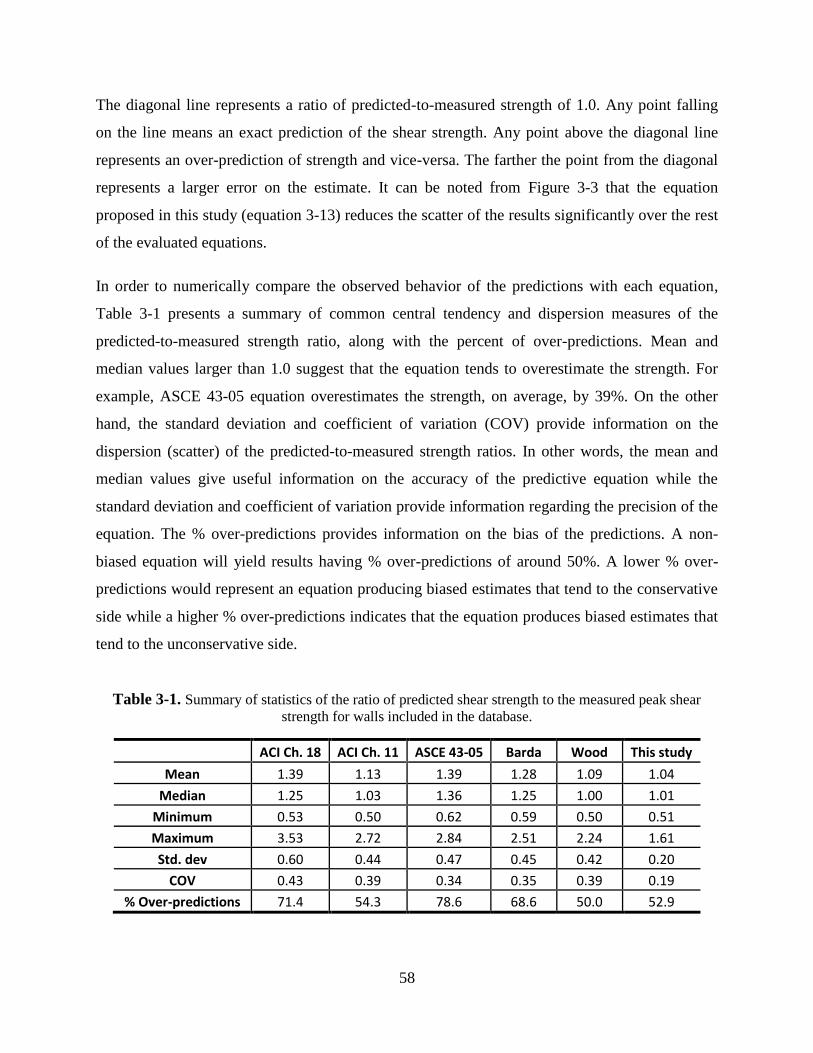
58

The diagonal line represents a ratio of predicted-to-measured strength of 1.0. Any point falling

on the line means an exact prediction of the shear strength. Any point above the diagonal line

represents an over-prediction of strength and vice-versa. The farther the point from the diagonal

represents a larger error on the estimate. It can be noted from Figure 3-3 that the equation

proposed in this study (equation 3-13) reduces the scatter of the results significantly over the rest

of the evaluated equations.

In order to numerically compare the observed behavior of the predictions with each equation,

Table 3-1 presents a summary of common central tendency and dispersion measures of the

predicted-to-measured strength ratio, along with the percent of over-predictions. Mean and

median values larger than 1.0 suggest that the equation tends to overestimate the strength. For

example, ASCE 43-05 equation overestimates the strength, on average, by 39%. On the other

hand, the standard deviation and coefficient of variation (COV) provide information on the

dispersion (scatter) of the predicted-to-measured strength ratios. In other words, the mean and

median values give useful information on the accuracy of the predictive equation while the

standard deviation and coefficient of variation provide information regarding the precision of the

equation. The % over-predictions provides information on the bias of the predictions. A non-

biased equation will yield results having % over-predictions of around 50%. A lower % over-

predictions would represent an equation producing biased estimates that tend to the conservative

side while a higher % over-predictions indicates that the equation produces biased estimates that

tend to the unconservative side.

Table 3-1. Summary of statistics of the ratio of predicted shear strength to the measured peak shear

strength for walls included in the database.

ACI Ch. 18 ACI Ch. 11 ASCE 43-05 Barda Wood This study

Mean 1.39 1.13 1.39 1.28 1.09 1.04

Median 1.25 1.03 1.36 1.25 1.00 1.01

Minimum 0.53 0.50 0.62 0.59 0.50 0.51

Maximum 3.53 2.72 2.84 2.51 2.24 1.61

Std. dev 0.60 0.44 0.47 0.45 0.42 0.20

COV 0.43 0.39 0.34 0.35 0.39 0.19

% Over-predictions 71.4 54.3 78.6 68.6 50.0 52.9

59

Figure 3-4 shows a typical box and whisker plot comparing the distribution of the predicted-to-

measured strength for each presented equation model. The graph shows the lower quartile (25th

percentile), median, upper quartile (75th percentile), the extreme values and the mean value

marked with “+” symbol. The box in the box and whisker plot is constituted by the second and

third quartile and represents the spread of the central 50% of the observations. The range of this

box is commonly known as the inter-quartile range (IQR), midspread, or middle fifty. The

narrower this range (or box in the graph) is, indicates the lesser the variability since the central

50% of the observations are nearer to the median value. The lower and upper whiskers of the

plot represent the spread of the first and fourth quartile, being the ends of the whiskers the

extreme (i.e. maximum and minimum) values marked with “-” tick mark.

Figure 3-4. Distribution of the ratio of predicted-to-measured peak strength.

It can be observed that the proposed equation produces a significantly improved estimate of the

shear strength since the mean and median values are very close to 1.0 and all the dispersion

measures indicate that the scatter is considerably reduced in comparison with the rest of the

evaluated equations. It is also observed that the midspread falls between 0.91 and 1.14, showing

the smallest IQR. Also, the range (difference between maximum and minimum values) has been

reduced, which suggests a reduction in scatter. In the same manner, the proposed equation yields

52.9% of over-predictions which is very near to the intended value. Note that ACI 318 Ch. 18,

ASCE 43-05 and Barda expressions tend to over-predict shear strength of squat walls with

0.00

0.50

1.00

1.50

2.00

2.50

3.00

3.50

4.00

0.00

0.50

1.00

1.50

2.00

2.50

3.00

3.50

4.00


Pre

dic

ted

str

en

gth

/ m

eas

ure

d s

tre

ngt

h

60

rectangular cross sections. This is observed on the box and whisker plot, central tendency

statistics, and on the high % over-predictions. Generally, an equation yielding mean and median

values near to 1.0 will produce nearly 50% over-predictions if the data is not severely skewed.

To further evaluate the proposed equation, a plot of the peak shear strength normalized with

𝐴𝑐𝑣√𝑓𝑐′ vs aspect ratio is presented in Figure 3-5. This figure shows that the upper strength limit

of the ACI 318-14 (0.83𝐴𝑐𝑣√𝑓𝑐′) is a reasonable value for squat shear walls with rectangular

cross sections. Thus, the use of this limit with the proposed equation 3-13 is recommended for

the estimation of peak shear strength. This limit has been traditionally imposed as an upper-

bound to avoid non-ductile diagonal compression failure in walls, wall piers, deep beams and

coupling beams. Figure 3-5 also suggests that the upper strength limit becomes more important

for walls of lower aspect ratios. In addition, a good correlation between the predicted and

measured normalized peak shear strengths can be noted.

Figure 3-5. Variation of the predicted and measured normalized peak shear strength with wall aspect

ratio compared to ACI 318 upper limit.

0.0

0.2

0.4

0.6

0.8

1.0

1.2

1.4

1.6

1.8

2.0

0.0 0.5 1.0 1.5 2.0

hw/lw

Measured

Calculated

ACI Upper Limit

61

DISPLACEMENT CAPACITY OF SQUAT

WALLS WITH RECTANGULAR CROSS

SECTION

4.1 Introduction

Many equations are found in current US design codes and literature for the prediction of the peak

shear strength of reinforced concrete walls. However, the available expressions for the prediction

of the displacement capacity of these structural systems are more limited. Current design codes

and standards usually provide fixed values for the allowable drift to control structural damage.

Duffey et al. (1994a, 1994b) found that design codes and standards tend to provide

unconservative drift limits for the case of low-rise RC walls as most of them are focused on high

rise buildings generally having slender walls. It has been generally accepted that squat walls tend

to exhibit brittle shear controlled failures while slender walls tend to fail in more ductile flexural

failure modes with less influence of shear deformations.

Some researchers (e.g. Hidalgo, 2000; Carrillo, 2010; Sánchez, 2013) have proposed different

expressions to calculate the displacement or drift capacity of squat RC walls based on calibration

against limited experimental data. While significant research has been performed during the past

years to address this situation, the development of better equations to assess the displacement

capacity of squat RC walls is still necessary. It is important to note that the scatter on the

predictions of displacement capacity is considerable. The accurate prediction of the displacement

capacity of squat walls is a challenging task since it involves several complex failure

mechanisms and other displacement sources, which are individually highly variable in nature.

Squat RC walls are commonly shear controlled elements and generally its load displacement

behavior does not show a clear yielding point. A major stiffness reduction is commonly observed

prior to peak strength development and followed by prompt strength degradation with relatively

low ductility. For structural analysis purposes, this behavior can be represented with a hysteretic

model using a tri-linear backbone curve. This chapter presents an evaluation of current

expressions for the prediction of the displacement capacity of squat reinforced concrete walls

62

with rectangular cross section found in the literature. The performance of each of the selected

equations was assessed by comparing the displacement predictions with experimental

displacements from the assembled database for walls with rectangular cross section. Key

parameters influencing the displacement capacity were identified. The experimental

displacements of each wall were taken as the average of the displacements measured from the

first and third quadrants (i.e. positive and negative loading directions, respectively). New

equations to predict the displacement capacities of squat walls at diagonal cracking, peak

strength, and ultimate state, are presented to improve current displacement estimates. These

displacement capacity estimates, in conjunction with the peak strength estimate presented in

Chapter 3 can be used to define the backbone curve for a hysteretic model. The equations were

obtained from multivariable linear regression analyses using an assembled experimental database

from various experimental programs which is presented on Chapter 2 and Appendix A. The

expressions presented herein are intended to apply for squat walls with rectangular cross section

and a wide range of characteristics.

4.2 Current Expressions for Estimation of Displacement Capacity

The following subsections discuss the selected current equations for displacement capacity

prediction. The equations shown are similar to those presented on the corresponding references

but the names and subscripts of the parameters have been modified to maintain uniformity within

equations, database and script throughout this document.

4.2.1 Hidalgo et al. (2000)

Hidalgo et al. (2000) developed a hysteretic model for the analysis of cyclic lateral load-

displacement behavior of squat RC shearwalls. The authors used a tri-linear hysteresis envelope

and proposed the following equations for the estimation of the drift at shear cracking, peak

strength, and the ultimate drift, based on linear regression from experimental results.

w

w

cr hVl

M

00175.0 for 0.1wVlM

(4-1)

63

w

w

cr hVl

M

0002.000155.0 for 0.1wVlM

(4-2)

w

w

peak hVl

M

0033.00027.0 for 0.1wVlM

(4-3)

w

w

peak hVl

M

00033.00056.0 for 0.1wVlM

(4-4)

w

w

u hVl

M

012.0002.0 for 0.1wVlM

(4-5)

wu h014.0 for 0.1wVlM

(4-6)

Figure 4-1. Tri-linear backbone model proposed by Hidalgo et al. (2000).

The authors recommended to use the ACI 318 seismic design provisions for determining the

peak shear strength with slight modifications to increase the concrete strength coefficient (αc) for

walls with aspect ratios below 1.5 and taking the wall area (Acv) as the thickness times the

minimum of the wall length and wall height. Further information can be found on Hidalgo and

Jordán (1996). The shear force corresponding to the cracking point was recommended to be

64

taken as the concrete contribution to strength of the ACI 318 seismic provisions and using the

same recommendations as for peak strength. The ultimate displacement was defined as the

displacement associated to a 20% decrease in strength (80% Vpeak) after peak point.

4.2.2 Carrillo (2010)

Carrillo (2010) presented a tri-linear backbone model for the analysis of squat walls. The model

was based on the observations from an experimental program carried-out at Universidad

Nacional Autónoma de México (UNAM) which was focused on studying the seismic behavior of

squat RC walls representative of typical housing in several Latin American countries. In the

same manner as in Hidalgo et al. (2000), the model presented by Carrillo (2010) included a

stiffness reduction which was deemed to be associated to the occurrence of significant diagonal

web cracking. Model backbone shape is similar to the model presented by Hidalgo et al. (2000)

but different expressions for the estimation of the cracking, peak and ultimate points were

proposed (refer to Figure 4-1). Carrillo (2010) proposed the following equations to calculate the

drift ratio at diagonal cracking as a percentage:

wcr

crcr

hK

VR

100%

(4-7)

cvc

w

gc

w

cr

AGc

h

IEc

hK

21

3

3

1

(4-8)

where Vcr is the diagonal cracking strength, Kcr is the cracked stiffness of the wall considering

both flexural and shear deformations, Ig is the strong axis gross moment of inertia of the wall

cross section, Gc is the shear modulus of elasticity of concrete, Ec is the modulus of elasticity of

concrete, c1 is a factor to account for flexural stiffness reduction due to cracking, and c2 is a

factor to account for reduced shear stiffness due to cracking. Carrillo (2010) recommended

taking both stiffness modifiers equal to 0.5 to represent the cracked stiffness. For an uncracked

element both factors should be taken equal to 1.0.

65

Ultimate displacement was defined as the displacement associated to a 20% decrease in strength

(80% Vpeak) after peak point. Carrillo (2010) proposed the following equations to calculate the

drift ratio at peak strength and ultimate drift ratio as a percentage:

wVl

M

cw

peak

peak eft

VR

30.1

' 5200

1% (4-9)

wVl

M

cw

peak

u eft

VR

35.1

' 3650

1% (4-10)

The peak shear strength can be calculated with the equation proposed by Carrillo (2010) which

was based on calibration of the ACI 318 equation form against experimental data. The cracking

strength was assumed as the concrete contribution to strength. Further information can be found

on Carrillo (2010).

4.2.3 Sánchez (2013)

Sánchez (2013) proposed a backbone model similar to the proposed by Hidalgo et al. (2000) and

Carrillo (2010) but modified to include a first stiffness reduction due to flexural cracking and a

second stiffness reduction due to distributed diagonal cracking. An additional line segment to

represent the initial uncracked stiffness and the reduced stiffness after flexural cracking was

included. Based on the experimental results from RC shear walls with similar characteristics of

those used for housing in Mexico, Sánchez (2013) proposed equations to estimate the strength

and displacement at flexural cracking, diagonal cracking, peak strength and ultimate damage

state as shown in Figure 4-2. Further information regarding the strength estimates can be found

on Sánchez (2013).

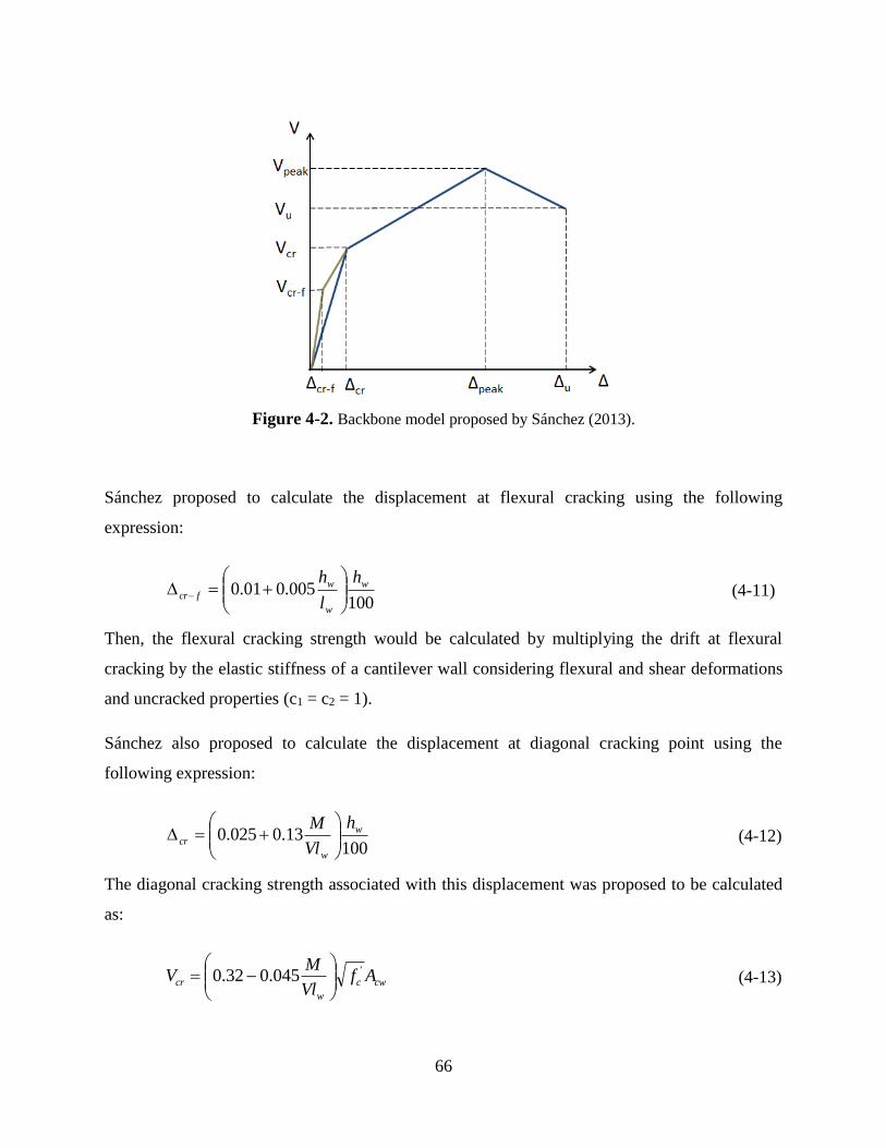
66

Figure 4-2. Backbone model proposed by Sánchez (2013).

Sánchez proposed to calculate the displacement at flexural cracking using the following

expression:

100

005.001.0 w

w

w

fcr

h

l

h

(4-11)

Then, the flexural cracking strength would be calculated by multiplying the drift at flexural

cracking by the elastic stiffness of a cantilever wall considering flexural and shear deformations

and uncracked properties (c1 = c2 = 1).

Sánchez also proposed to calculate the displacement at diagonal cracking point using the

following expression:

100

13.0025.0 w

w

cr

h

Vl

M

(4-12)

The diagonal cracking strength associated with this displacement was proposed to be calculated

as:

cwc

w

cr AfVl

MV '045.032.0

(4-13)

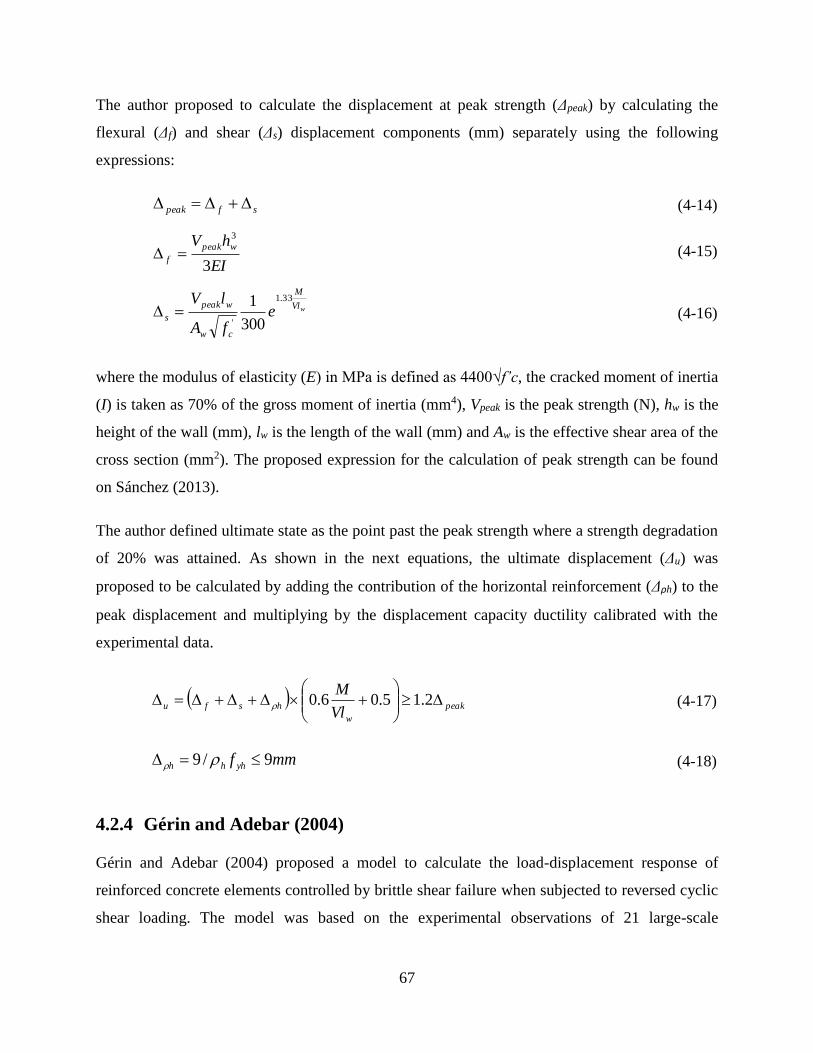
67

The author proposed to calculate the displacement at peak strength (Δpeak) by calculating the

flexural (Δf) and shear (Δs) displacement components (mm) separately using the following

expressions:

sfpeak (4-14)

EI

hV wpeak

f3

3

(4-15)

wVl

M

cw

wpeak

s efA

lV 33.1

' 300

1 (4-16)

where the modulus of elasticity (E) in MPa is defined as 4400√f’c, the cracked moment of inertia

(I) is taken as 70% of the gross moment of inertia (mm4), Vpeak is the peak strength (N), hw is the

height of the wall (mm), lw is the length of the wall (mm) and Aw is the effective shear area of the

cross section (mm2). The proposed expression for the calculation of peak strength can be found

on Sánchez (2013).

The author defined ultimate state as the point past the peak strength where a strength degradation

of 20% was attained. As shown in the next equations, the ultimate displacement (Δu) was

proposed to be calculated by adding the contribution of the horizontal reinforcement (Δρh) to the

peak displacement and multiplying by the displacement capacity ductility calibrated with the

experimental data.

peak

w

hsfuVl

M

2.15.06.0 (4-17)

mmf yhhh 9/9 (4-18)

4.2.4 Gérin and Adebar (2004)

Gérin and Adebar (2004) proposed a model to calculate the load-displacement response of

reinforced concrete elements controlled by brittle shear failure when subjected to reversed cyclic

shear loading. The model was based on the experimental observations of 21 large-scale

68

membrane-type element tests. The backbone curve of the model can be represented by the curve

shown on the following figure.

Figure 4-3. Backbone model proposed by Gérin and Adebar (2004).

The stress (vcr) and shear strain (γcr) at shear cracking were proposed to be calculated with the

following expressions:

cr

vcrcr

ffv

1 (4-19)

c

cr

crG

v (4-20)

'33.0 ccr ff (4-21)

cc EG 4.0 (4-22)

where fcr is the concrete tensile cracking stress, σv is the vertical axial stress (positive sign for

compression), Gc is the uncracked shear modulus of elasticity of concrete and Ec is the modulus

of elasticity of concrete.

On this model the yield (peak) stress (vy) is recommended to be calculated per ACI 318-08 and

the shear strain at yield (shear strain at peak strength - γy) is calculated using the following

equation:

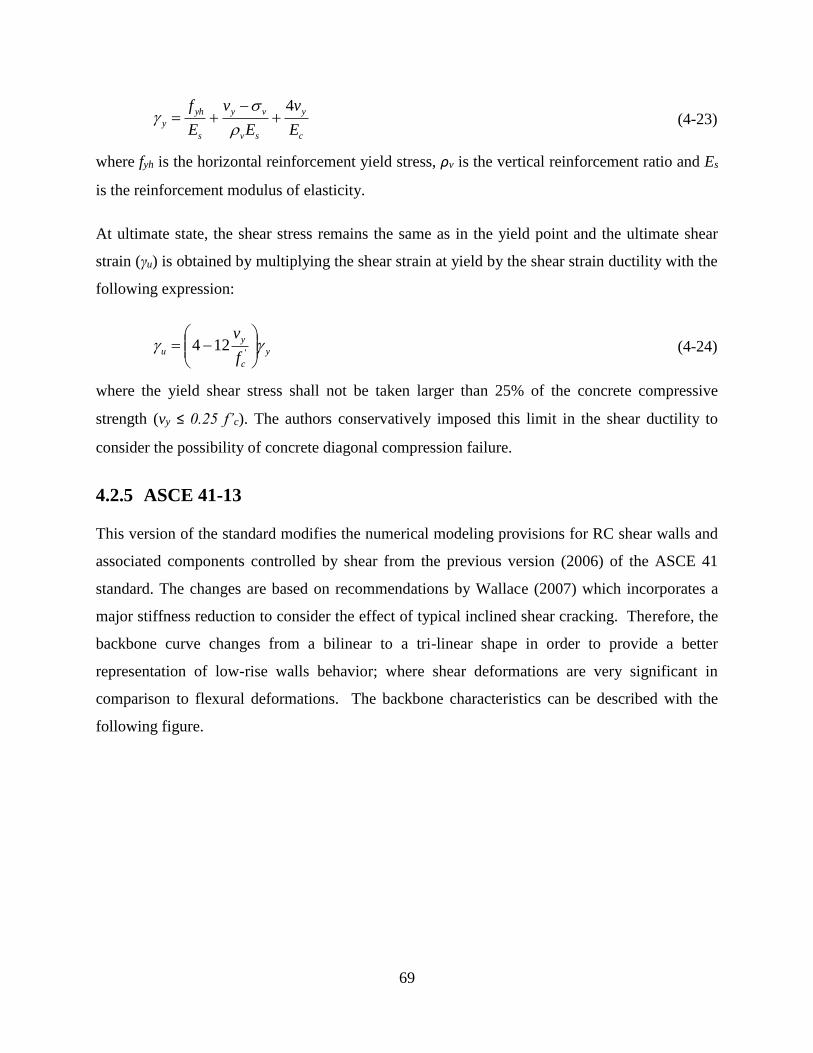
69

c

y

sv

vy

s

yh

yE

v

E

v

E

f 4

(4-23)

where fyh is the horizontal reinforcement yield stress, ρv is the vertical reinforcement ratio and Es

is the reinforcement modulus of elasticity.

At ultimate state, the shear stress remains the same as in the yield point and the ultimate shear

strain (γu) is obtained by multiplying the shear strain at yield by the shear strain ductility with the

following expression:

y

c

y

uf

v

'124 (4-24)

where the yield shear stress shall not be taken larger than 25% of the concrete compressive

strength (vy ≤ 0.25 f’c). The authors conservatively imposed this limit in the shear ductility to

consider the possibility of concrete diagonal compression failure.

4.2.5 ASCE 41-13

This version of the standard modifies the numerical modeling provisions for RC shear walls and

associated components controlled by shear from the previous version (2006) of the ASCE 41

standard. The changes are based on recommendations by Wallace (2007) which incorporates a

major stiffness reduction to consider the effect of typical inclined shear cracking. Therefore, the

backbone curve changes from a bilinear to a tri-linear shape in order to provide a better

representation of low-rise walls behavior; where shear deformations are very significant in

comparison to flexural deformations. The backbone characteristics can be described with the

following figure.

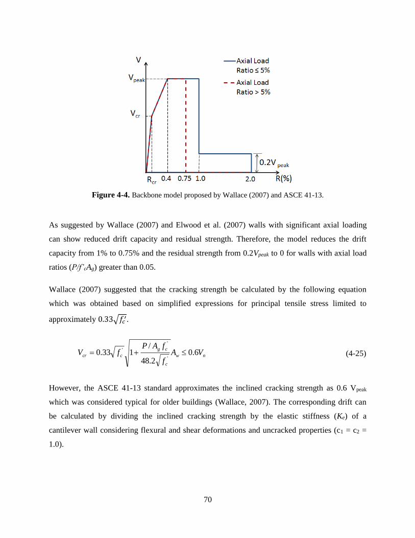
70

Figure 4-4. Backbone model proposed by Wallace (2007) and ASCE 41-13.

As suggested by Wallace (2007) and Elwood et al. (2007) walls with significant axial loading

can show reduced drift capacity and residual strength. Therefore, the model reduces the drift

capacity from 1% to 0.75% and the residual strength from 0.2Vpeak to 0 for walls with axial load

ratios (P/f’cAg) greater than 0.05.

Wallace (2007) suggested that the cracking strength be calculated by the following equation

which was obtained based on simplified expressions for principal tensile stress limited to

approximately 0.33√𝑓𝑐′.

nw

c

cg

ccr VAf

fAPfV 6.0

2.48

/133.0

'

'

' (4-25)

However, the ASCE 41-13 standard approximates the inclined cracking strength as 0.6 Vpeak

which was considered typical for older buildings (Wallace, 2007). The corresponding drift can

be calculated by dividing the inclined cracking strength by the elastic stiffness (Ke) of a

cantilever wall considering flexural and shear deformations and uncracked properties (c1 = c2 =

1.0).

71

4.2.6 Duffey et al. (1994a, 1994b)

Duffey et al. (1994a, 1994b) suggested average values for drift ratio at peak strength and at

several stages of strength degradation past the peak strength, based on statistical analysis of

experimental data compiled from numerous experimental studies. They found mean and median

drift ratio at peak strength of 0.80% and 0.72%, respectively. The authors also published the

central tendency values for subsequent damage stages such as attaining 90, 80, 70, 60 and 50%

of the peak strength. However, the authors stated that care must be exercised when modelling

using values of drift beyond the peak strength since relatively small energy dissipation capacity

may remain in the wall (due to rapid strength and stiffness degradation) while the earthquake

motion may still impart significant energy. Even though some walls may have enough energy

dissipation capacity after attaining peak strength, data for this advanced damage stage was

scarcer since many of the early experimental studies presented data only up to the peak load.

Therefore, they recommended using the drift ratio values associated to the peak strength as the

ultimate drift capacity when performing analyses using hysteretic models. Duffey et al. (1994a,

1994b) also noted that the allowable drift limits on most design codes and standards tend to be

unconservative for low-rise RC shearwalls because those are mainly focused on high rise

buildings comprised of slender walls which generally have higher ductility.

4.3 Development of New Displacement Capacity Predictive

Equations

The experimental load-displacement envelope of these type of shear-controlled walls does not

typically show a clear yielding point, but major stiffness reduction is generally observed prior to

the peak strength, and the post-peak response is characterized by rapid strength degradation

showing relatively low ductility (see Figure 4-5). For structural analysis purposes, this behavior

can be represented with a hysteretic model using a tri-linear backbone curve (see Figure 4-1).

Drift data was collected from numerous experiments found in literature and were included in the

assembled database. The availability of displacement data is more limited than peak strength data

since not all the references included in this study included displacements, drift or global force-

displacement data. Drift data collection was possible for 63 of the 70 specimens with rectangular

cross section listed in the database (Appendix A). The drift data for the ultimate state (20%

72

strength drop) was even scarcer since many of the early experimental studies presented data only

up to the peak load. Therefore, only 58 qualifying datasets of ultimate drift could be obtained

from the evaluated references for walls with rectangular cross section.

Most of the data was obtained from global force-displacement hysteresis curves found on the

evaluated references. Therefore, it considers the total drift instead of separate shear and flexural

displacement components. The vast majority of cyclic tests were displacement controlled, where

the wall specimen is loaded to a specific displacement in one direction, then the load is reversed

to the same displacement in the opposite direction. Typically, specimens were subjected to

several load reversal cycles (2 or 3) at the same displacement level as shown on Figure 4-5. In

order to obtain the drift data, first, the cyclic envelope was traced from the hysteresis curves, and

the displacement data was converted to drift ratio (taken as the ratio between the lateral

displacement to height where displacement was measured). Straight lines connecting the peaks

of the first cycle at each displacement level were used to trace the experimental envelope (see

Figure 4-5). The load-displacement envelope was not extrapolated further than the last loading

peaks. Afterwards, the drift ratios corresponding to the assumed diagonal cracking condition

(Rcr), peak strength (Rpeak) and at ultimate state (Ru) were retrieved from the obtained cyclic

envelope. The average drift ratio from 1st and 3rd quadrants of each wall were recorded for each

of the three states. Cracking drift ratio was defined as that corresponding to the development of

60% of peak strength, while ultimate drift ratio was defined as that corresponding to the post-

peak point where a strength degradation of 20% is attained. Further details are discussed in the

next sub-sections. For tests where ultimate displacement data was not available for one of the

loading directions (commonly when test is stopped due to sudden failure in the opposite

direction), the single value available for the ultimate displacement was recorded.

73

Figure 4-5. Representative experimental load-displacement envelope (adapted from Palermo and

Vecchio, 2002).

Regression analyses were performed to develop empirical equations that better fits the collected

drift data. The goal was to lower the coefficient of variation and to obtain a mean value near to

1.0 for the ratio of predicted-to-measured drift capacity. Key parameters were identified by

evaluating the correlation coefficient with the drift capacity. The correlation coefficient can

range from 0 to 1.0 and indicates the degree of linear relationship between two variables. A

correlation coefficient with a value of 1 indicates a perfect correlation while a value of 0

indicates that no correlation exists. Multivariable linear regression analyses were carried to

derive the equations with the selected parameters. In order to simplify the equations, the least

meaningful parameters were eliminated (one at a time), based on the highest p-value, and the

equation was recalibrated by regression. This process was repeated until the scatter of the

prediction was observed to increase. In order to minimize bias due to test specimens’ scale, the

collected displacement data was converted to drift ratio, reinforcement spacing was normalized

with wall thickness and any parameter involving forces was normalized with the effective shear

area of the section (Acv) for the calibration and development of equations. The following sub-

74

sections present the simplified expressions using the most significant parameters that were found

to produce a better correlation with the database, and are proposed for the prediction of drift ratio

at diagonal cracking, drift ratio at peak strength and at ultimate drift ratio, respectively.

4.3.1 Drift Ratio at Diagonal Cracking

Researchers have used different approaches to estimate the point at which the first main stiffness

reduction occurs. It has been reported by some researchers (e.g. Salonikios et al., 2000; Carrillo,

2010; and Greifenhagen and Lestuzzi, 2005) that first significant yield generally occurred close

to the development of 75 to 80% of the maximum lateral strength of RC squat walls specimens.

However, most researchers coincide on the assumption that the first major stiffness decrease is

related to the occurrence of significant inclined cracking across the web with enough crack width

as to start mobilizing a shear friction mechanism through crack surfaces. Carrillo and Alcocer

(2012) suggested that distributed diagonal cracking occurs at a lateral load higher than that

associated with the first inclined web crack and that it generally occur at load levels lower than

that associated with onset yielding of reinforcement. Carrillo and Alcocer (2012) also proposed

to assume the cracking shear equal to the concrete contribution to shear strength.

Sánchez (2013) points out that the first significant diagonal cracking does not cover the whole

length of the wall and the typical crack width at this stage is in the order of 0.3 mm to 0.6 mm.

Therefore, Sánchez (2013) defined the significant diagonal cracking strength as the lateral force

at which the cracks have widened to 0.5 mm and cracking covers 40% of the wall length.

Calibrated expressions for the cracking strength and cracking drift based on experimental

observations were proposed by Sánchez (2013).

Wallace (2007) suggested modifications to the ASCE 41-06 standard to include a point of

stiffness reduction associated to the concrete diagonal cracking into the backbone curves for

shear-controlled walls and wall segments, and recommended an expression to calculate the

cracking strength. ASCE 41-13 incorporated the recommendations by Wallace (2007) and

provides fixed drift ratio values for determining the drift capacities, but allows the cracking

strength to be taken as 60% of the peak strength.

75

For the purpose of simplicity, it was assumed in this study that both, the significant inclined

cracking and ultimate damage states occur at a fixed portion of the peak strength. In order to

better represent the squat shear walls behavior, two options for the estimation of the cracking or

“first yield” point were considered. In the first option, the main decrease in stiffness was

assumed to occur upon loading to 60% of peak strength, which has been considered to be the

typical lateral force associated to significant inclined cracking (Wallace, 2007 and ASCE 41-13).

On the second option, it was assumed that the main stiffness reduction occurs upon loading to

75% of the peak strength which could be representative of the onset reinforcement yielding. The

definition of the first stiffness reduction point, based on the 60% of the peak strength (diagonal

cracking), was found to generally better approximate the ascending branch of the experimental

envelope and the initial stiffness. Therefore, the cracking drift equation was fitted based on the

assumption that significant web cracking occurs at the point where 60% of the maximum

strength is attained. The parameter selection and equation calibration approach by multiple linear

regression analyses was described on previous section (4.3). The following simplified

expression includes the most significant parameters that were found to produce a better

correlation with the database and is proposed for the prediction of drift ratio at significant

diagonal cracking state (Rcr) of squat RC walls with rectangular cross section.

w

w

hbecrt

lR 000024.0093.0124.00006.0 (4-26)

where ρbe is the boundary element reinforcement ratio (Asbe/Acv), ρh is the horizontal

reinforcement ratio, lw is the wall length and hw is the wall height.

4.3.2 Drift Ratio at Peak Strength

Different approaches to obtain the displacement capacity at peak strength have been used in

other studies presented earlier. Carrillo (2010) and Sánchez (2013) calibrated their displacement

capacity at peak strength expressions based on the observed peak strength and the moment-to-

shear span ratio as main predictive parameters. Gérin and Adebar (2004) used a theoretical

mechanics approach to determine the shear strain at peak strength. Hidalgo et al. (2000) used the

moment-to-shear span ratio as the only predictive parameter for their expressions. ASCE 41-13

establishes a typical fixed value for the estimation of displacement at peak strength.

76

Based on the observed approaches made by other researchers, two main options were evaluated

in this study for the development of equations to estimate the displacement capacity at peak

strength of squat RC walls with rectangular cross section. The first option considered that the

peak shear strength was an influential parameter on the displacement at peak strength, while

other parameters were selected based on the correlation coefficient. On the second option, all the

influential parameters were preliminarily selected based on their correlation coefficient with the

displacement data. In both options the same general approach in terms of the iterative process of

simplifying the equations by eliminating the least meaningful parameters based on the p-value as

described earlier was employed.

While some researchers have found that the peak strength is a good predictive parameter, no

strong correlation between the peak strength and the displacement at peak strength was found in

the database included in this study. The following simplified equation includes the parameters

found to produce a better correlation with experimental data considered in this study; and is

proposed for the estimation of the drift ratio at peak strength (Rpeak) of squat RC walls with

rectangular cross sections.

w

h

cyhpeakt

sffR 00044.0000063.0000006.00094.0 ' (4-27)

where fyh is the horizontal reinforcement yield stress (MPa), f’c is the concrete compressive

strength (MPa), sh is the horizontal reinforcement spacing (mm), and tw is the wall thickness

(mm).

4.3.3 Drift Ratio at Ultimate Damage State

The ultimate drift equation was fitted based on the definition of ultimate damage state as the

point where the strength degrades to attain 80% of the peak strength. Similar assumptions have

been used by numerous researchers to define the ultimate damage state. Kazaz et al. (2012)

defined ultimate state as the point on the load-deformation curve where strength drops abruptly

or degrades to 85% of the maximum strength. Several researchers (i.e. Sánchez, 2013; Carrillo,

2010; Kuang and Ho, 2008; Greifenhagen and Lestuzzi, 2005; Hidalgo, 1996; Park, 1989;

among others) have defined the ultimate drift as that corresponding to a 20% strength drop after

77

peak strength. Salonikios et al. (2000) defined the ultimate damage state when the strength has

dropped 25% of the peak strength. This ultimate state criterion has been conventionally used for

RC walls and other type of concrete members subject to lateral loading.

Regarding the estimation of displacement capacity at ultimate state, different approaches have

been used by other researchers as well. Carrillo (2010) based his estimated capacity on he

observed peak strength and the moment-to-shear span ratio. Sánchez (2013) and Gérin and

Adebar (2004) used a calibrated ductility expression to estimate the ultimate displacement.

Hidalgo et al. (2000) used the moment-to-shear span ratio as the only predictive parameter for

the ultimate drift capacity. ASCE 41-13 establishes a typical fixed value for the estimation of

ultimate drift capacity for walls with low axial load ratio and for walls with significant axial load

ratio, respectively.

In a similar fashion as for the displacement at peak strength, several options using multiple linear

regressions were evaluated in this study. The two options used for the displacement at peak

strength (i.e. considering a term related to the peak strength, and considering other parameters

but peak strength) were evaluated for the ultimate displacement as well. An additional option

based on the calibration of the observed displacement ductility (Δu/Δpeak) was considered for this

damage state. The same iterative approach for parameters selection and simplification of the final

equation described on earlier sections was used herein for all three options.

The following expression is proposed for the estimation of ultimate displacement (Ru) of squat

RC walls with rectangular cross section in terms of drift ratio:

peak

gw

v

w

h

vu RA

P

t

s

t

sR 001.00042.00046.0302.0013.0 (4-28)

where ρv is the vertical reinforcement ratio, sh is the horizontal reinforcement spacing (mm), sv is

the vertical reinforcement spacing (mm), P is the axial load (N), and Ag is the gross cross

sectional area (mm2).

78

4.4 Evaluation of Selected Displacement Capacity Equations

In this section the selected predictive equations found in literature and the new expressions

developed herein were evaluated in terms of their predictive performance by using a statistical

analysis approach and comparing to the experimental data compiled in the assembled database

(Appendix A). In order to minimize bias due to test specimens scale, all the displacement

predictions were converted to drift ratio for comparison.

The following subsections show detailed analysis of the performance of each of the equations

developed in this study for each of the three defined damage states, and compares them to the

performance of the corresponding equations found in literature. Tabulated summaries of

common central tendency and dispersion measures of the predicted-to-measured drift ratios,

along with the percent of over-predictions, are presented in the same fashion as presented on

Chapter 3 for the strength predictions. Mean and median values larger than 1.0 suggest that the

equation tends to overestimate the drift ratio. On the other hand, the standard deviation and

coefficient of variation (COV) provide information on the dispersion (scatter) of the predicted-

to-measured drift ratio. In other words, the mean and median values give useful information on

the accuracy of the predictive equation while the standard deviation and coefficient of variation

provide information regarding the precision of the equation. The % over-predictions provides

information on the bias of the predictions. A non-biased equation will yield results having %

over-predictions of around 50%. A lower % of over-predictions would represent an equation

producing biased estimates that tend to underestimate drift ratios, while a higher % of over-

predictions indicates that the equation produces biased estimates that tend to overestimate drift

ratios.

Sections 4.4.1, 4.4.2 and 4.4.3 will discuss the findings for the displacement at diagonal

cracking, displacement at peak strength and ultimate displacement, respectively.


The performance of the equations for the prediction of the cracking or “first yield” displacement

will not be compared as all of them are based on different assumptions of the corresponding

strength at which the stiffness reduction occurs, and therefore, are not directly comparable. Thus,

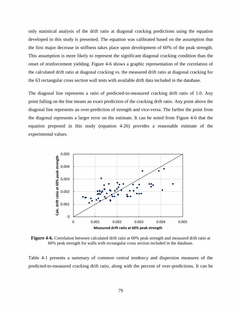
79

only statistical analysis of the drift ratio at diagonal cracking predictions using the equation

developed in this study is presented. The equation was calibrated based on the assumption that

the first major decrease in stiffness takes place upon development of 60% of the peak strength.

This assumption is more likely to represent the significant diagonal cracking condition than the

onset of reinforcement yielding. Figure 4-6 shows a graphic representation of the correlation of

the calculated drift ratio at diagonal cracking vs. the measured drift ratio at diagonal cracking for

the 63 rectangular cross section wall tests with available drift data included in the database.

The diagonal line represents a ratio of predicted-to-measured cracking drift ratio of 1.0. Any

point falling on the line means an exact prediction of the cracking drift ratio. Any point above the

diagonal line represents an over-prediction of strength and vice-versa. The farther the point from

the diagonal represents a larger error on the estimate. It can be noted from Figure 4-6 that the

equation proposed in this study (equation 4-26) provides a reasonable estimate of the

experimental values.

Figure 4-6. Correlation between calculated drift ratio at 60% peak strength and measured drift ratio at

60% peak strength for walls with rectangular cross section included in the database.


predicted-to-measured cracking drift ratio, along with the percent of over-predictions. It can be

0

0.001

0.002

0.003

0.004

0.005

0 0.001 0.002 0.003 0.004 0.005

Cal

c. d

rift

rat

io a

t 6

0%

pe

ak s

tre

ngt

h

Measured drift ratio at 60% peak strength

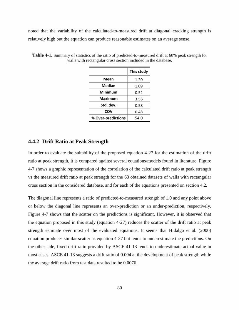
80

noted that the variability of the calculated-to-measured drift at diagonal cracking strength is

relatively high but the equation can produce reasonable estimates on an average sense.

Table 4-1. Summary of statistics of the ratio of predicted-to-measured drift at 60% peak strength for

walls with rectangular cross section included in the database.

This study

Mean 1.20

Median 1.09

Minimum 0.52

Maximum 3.56

Std. dev. 0.58

COV 0.48

% Over-predictions 54.0


In order to evaluate the suitability of the proposed equation 4-27 for the estimation of the drift

ratio at peak strength, it is compared against several equations/models found in literature. Figure

4-7 shows a graphic representation of the correlation of the calculated drift ratio at peak strength

vs the measured drift ratio at peak strength for the 63 obtained datasets of walls with rectangular

cross section in the considered database, and for each of the equations presented on section 4.2.

The diagonal line represents a ratio of predicted-to-measured strength of 1.0 and any point above

or below the diagonal line represents an over-prediction or an under-prediction, respectively.

Figure 4-7 shows that the scatter on the predictions is significant. However, it is observed that

the equation proposed in this study (equation 4-27) reduces the scatter of the drift ratio at peak

strength estimate over most of the evaluated equations. It seems that Hidalgo et al. (2000)

equation produces similar scatter as equation 4-27 but tends to underestimate the predictions. On

the other side, fixed drift ratio provided by ASCE 41-13 tends to underestimate actual value in

most cases. ASCE 41-13 suggests a drift ratio of 0.004 at the development of peak strength while

the average drift ratio from test data resulted to be 0.0076.

81

Figure 4-7. Correlation between calculated drift ratio at peak strength and measured drift ratio at peak

strength using various available equations: (a) to (e); and the new equation proposed in this study (f).

0

0.005

0.01

0.015

0.02

0.000 0.005 0.010 0.015 0.020

Cal

c. d

rift

rat

io a

t p

eak

str

en

gth

Measured drift ratio at peak strength

(a) Hidalgo et al.

0

0.005

0.01

0.015

0.02

0 0.005 0.01 0.015 0.02

Cal

c. d

rift

rat

io a

t p

eak

str

en

gth


(b) Carrillo

0

0.005

0.01

0.015

0.02

0 0.005 0.01 0.015 0.02

Cal

c. d

rift

rat

io a

t p

eak

str

en

gth


(c) Sánchez

0

0.005

0.01

0.015

0.02

0 0.005 0.01 0.015 0.02

Cal

c. d

rift

rat

io a

t p

eak

str

en

gth


(d) Gérin & Adebar

0

0.005

0.01

0.015

0.02

0 0.005 0.01 0.015 0.02

Cal

c. d

rift

rat

io a

t p

eak

str

en

gth


(e) ASCE 41-13

0

0.005

0.01

0.015

0.02

0 0.005 0.01 0.015 0.02

Cal

c. d

rift

rat

io a

t p

eak

str

en

gth


(f) This study

82

In order to numerically compare the predictive performance of each equation, Table 4-2 presents

a summary of common central tendency and dispersion measures of the predicted-to-measured

drift ratio at peak strength, along with the percent of over-predictions. Figure 4-8 shows a typical

box and whisker plot comparing the distribution of the predicted-to-measured drift ratio for each

selected equations/models. The graph shows the lower quartile (25th percentile), median, upper

quartile (75th percentile), the extreme values and the mean value marked with “+” symbol. The

central box in the box and whisker plot is constituted by the second and third quartile and

represents the spread of the central 50% of the observations. The range of this box is commonly

known as the inter-quartile range (IQR), midspread or middle fifty. The narrower this range (or

box in the graph) is, indicates the lesser the variability since the central 50% of the observations

are nearer to the median value. The lower and upper whiskers of the plot represent the spread of

the first and fourth quartile, being the ends of the whiskers the extreme (i.e. maximum and

minimum) values marked with “-” tick mark.

Table 4-2. Summary of statistics of the ratio of predicted-to-measured drift at peak strength for walls

with rectangular cross section included in the database.

Hidalgo et al. Carrillo Sánchez Gérin & Adebar ASCE 41-13 This study

Mean 0.78 0.90 1.14 0.77 0.59 1.11

Median 0.67 0.87 1.19 0.70 0.56 1.08

Minimum 0.31 0.30 0.36 0.17 0.28 0.54

Maximum 1.52 1.84 3.23 1.58 1.12 2.13

Std. dev. 0.29 0.38 0.50 0.33 0.21 0.36

COV 0.38 0.42 0.44 0.42 0.35 0.33


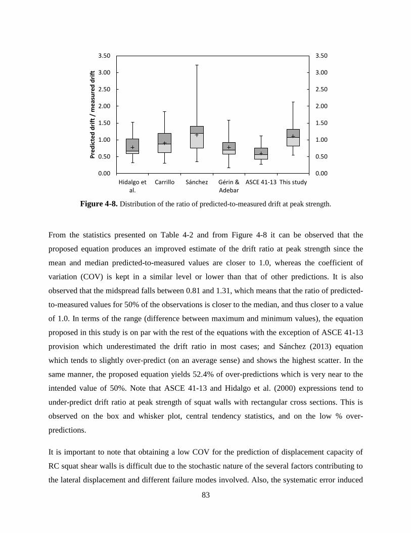
83

Figure 4-8. Distribution of the ratio of predicted-to-measured drift at peak strength.

From the statistics presented on Table 4-2 and from Figure 4-8 it can be observed that the

proposed equation produces an improved estimate of the drift ratio at peak strength since the

mean and median predicted-to-measured values are closer to 1.0, whereas the coefficient of

variation (COV) is kept in a similar level or lower than that of other predictions. It is also

observed that the midspread falls between 0.81 and 1.31, which means that the ratio of predicted-

to-measured values for 50% of the observations is closer to the median, and thus closer to a value

of 1.0. In terms of the range (difference between maximum and minimum values), the equation

proposed in this study is on par with the rest of the equations with the exception of ASCE 41-13

provision which underestimated the drift ratio in most cases; and Sánchez (2013) equation

which tends to slightly over-predict (on an average sense) and shows the highest scatter. In the

same manner, the proposed equation yields 52.4% of over-predictions which is very near to the

intended value of 50%. Note that ASCE 41-13 and Hidalgo et al. (2000) expressions tend to

under-predict drift ratio at peak strength of squat walls with rectangular cross sections. This is

observed on the box and whisker plot, central tendency statistics, and on the low % over-

predictions.

It is important to note that obtaining a low COV for the prediction of displacement capacity of

RC squat shear walls is difficult due to the stochastic nature of the several factors contributing to

the lateral displacement and different failure modes involved. Also, the systematic error induced

0.00

0.50

1.00

1.50

2.00

2.50

3.00

3.50

0.00

0.50

1.00

1.50

2.00

2.50

3.00

3.50

Hidalgo etal.

Carrillo Sánchez Gérin &Adebar

ASCE 41-13 This study

Pre

dic

ted

dri

ft /

me

asu

red

dri

ft

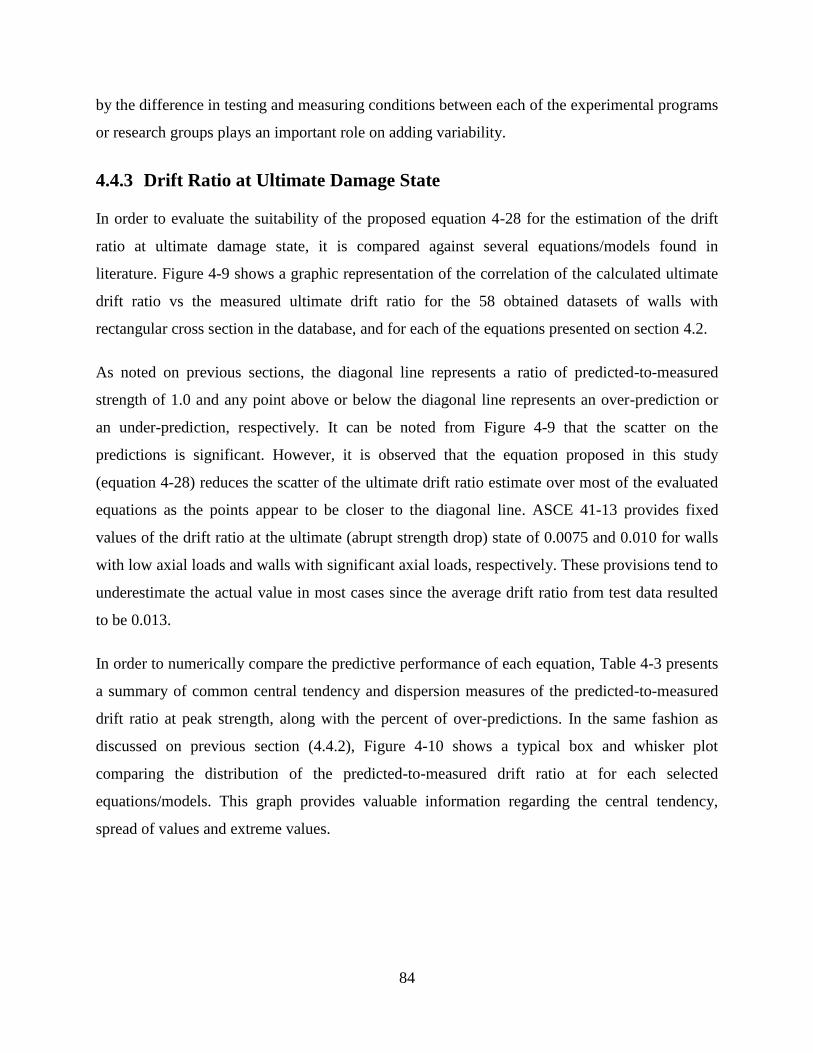
84

by the difference in testing and measuring conditions between each of the experimental programs

or research groups plays an important role on adding variability.



ratio at ultimate damage state, it is compared against several equations/models found in

literature. Figure 4-9 shows a graphic representation of the correlation of the calculated ultimate

drift ratio vs the measured ultimate drift ratio for the 58 obtained datasets of walls with

rectangular cross section in the database, and for each of the equations presented on section 4.2.

As noted on previous sections, the diagonal line represents a ratio of predicted-to-measured

strength of 1.0 and any point above or below the diagonal line represents an over-prediction or

an under-prediction, respectively. It can be noted from Figure 4-9 that the scatter on the

predictions is significant. However, it is observed that the equation proposed in this study

(equation 4-28) reduces the scatter of the ultimate drift ratio estimate over most of the evaluated

equations as the points appear to be closer to the diagonal line. ASCE 41-13 provides fixed

values of the drift ratio at the ultimate (abrupt strength drop) state of 0.0075 and 0.010 for walls

with low axial loads and walls with significant axial loads, respectively. These provisions tend to

underestimate the actual value in most cases since the average drift ratio from test data resulted

to be 0.013.



drift ratio at peak strength, along with the percent of over-predictions. In the same fashion as

discussed on previous section (4.4.2), Figure 4-10 shows a typical box and whisker plot

comparing the distribution of the predicted-to-measured drift ratio at for each selected

equations/models. This graph provides valuable information regarding the central tendency,

spread of values and extreme values.

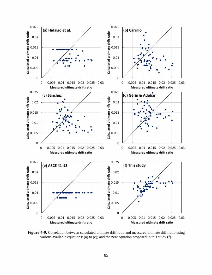
85

Figure 4-9. Correlation between calculated ultimate drift ratio and measured ultimate drift ratio using


0

0.005

0.01

0.015

0.02

0.025

0 0.005 0.01 0.015 0.02 0.025 0.03

Cal

cula

ted

ult

imat

e d

rift

rat

io

Measured ultimate drift ratio

(a) Hidalgo et al.

0

0.005

0.01

0.015

0.02

0.025

0 0.005 0.01 0.015 0.02 0.025 0.03

Cal

cula

ted

ult

imat

e d

rift

rat

io


(b) Carrillo

0

0.005

0.01

0.015

0.02

0.025

0 0.005 0.01 0.015 0.02 0.025 0.03

Cal

cula

ted

ult

imat

e d

rift

rat

io


(c) Sánchez

0

0.005

0.01

0.015

0.02

0.025

0 0.005 0.01 0.015 0.02 0.025 0.03

Cal

cula

ted

ult

imat

e d

rift

rat

io


(d) Gérin & Adebar

0

0.005

0.01

0.015

0.02

0.025

0 0.005 0.01 0.015 0.02 0.025 0.03

Cal

cula

ted

ult

imat

e d

rift

rat

io


(e) ASCE 41-13

0

0.005

0.01

0.015

0.02

0.025

0 0.005 0.01 0.015 0.02 0.025 0.03

Cal

cula

ted

ult

imat

e d

rift

rat

io


(f) This study

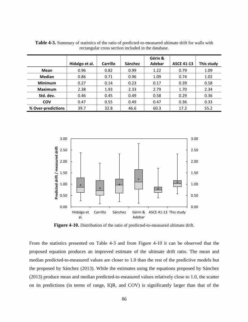
86

Table 4-3. Summary of statistics of the ratio of predicted-to-measured ultimate drift for walls with

rectangular cross section included in the database.


Mean 0.96 0.82 0.99 1.22 0.79 1.09

Median 0.86 0.71 0.96 1.09 0.74 1.02

Minimum 0.27 0.14 0.23 0.17 0.39 0.58

Maximum 2.38 1.93 2.33 2.79 1.70 2.34

Std. dev. 0.46 0.45 0.49 0.58 0.29 0.36

COV 0.47 0.55 0.49 0.47 0.36 0.33


Figure 4-10. Distribution of the ratio of predicted-to-measured ultimate drift.

From the statistics presented on Table 4-3 and from Figure 4-10 it can be observed that the

proposed equation produces an improved estimate of the ultimate drift ratio. The mean and

median predicted-to-measured values are closer to 1.0 than the rest of the predictive models but

the proposed by Sánchez (2013). While the estimates using the equations proposed by Sánchez

(2013) produce mean and median predicted-to-measured values relatively close to 1.0, the scatter

on its predictions (in terms of range, IQR, and COV) is significantly larger than that of the

0.00

0.50

1.00

1.50

2.00

2.50

3.00

0.00

0.50

1.00

1.50

2.00

2.50

3.00

Hidalgo etal.



Pre

dic

ted

dri

ft /

me

asu

red

dri

ft

87

equation proposed in this study. Similarly, the equation 4-28 (this study) produced lower COV of

the predicted-to-measured drift ratio than other predictions. It is also observed that the midspread

falls between 0.90 and 1.16, which means that the ratio of predicted-to-measured values for 50%

of the observations is closer to the median, and thus closer to a value of 1.0. In terms of the range

(difference between maximum and minimum values), the equation proposed in this study is on

par or narrower than the rest of the equations with the exception of ASCE 41-13 provision

which, in most cases, underestimated the drift ratio. This is observed on the box and whisker

plot, central tendency statistics, and on the low % over-predictions. The proposed equation yields

55.2% of over-predictions which is close to the intended value of 50%.

In the same manner as in the drift ratio at peak strength case, obtaining a low COV for the

prediction of displacement capacity of RC squat shear walls is challenging due to the stochastic

nature of the several factors contributing to the post-peak lateral displacement and the different

failure modes involved. Also, the systematic error induced by the difference in testing and

measuring conditions between each of the experimental programs or research groups appears to

be an influent source of variability.

On the other hand, drift limits have been conventionally imposed in building codes for the

purpose of controlling damage and as a measure of collapse prevention during an earthquake

event. The allowable drift ratios for RC shearwall building systems provided on most current

building design codes tend to be unconservative since they appear to be mainly focused on tall

buildings, where the main earthquake force resisting system commonly consists of slender

shearwalls. For example, ASCE 7-10 seismic provisions allow a drift ratio of 0.02, which is far

beyond the typical ultimate drift capacity of squat RC walls. The average ultimate drift ratio

obtained from the experimental values on the collected database of squat walls with rectangular

cross sections was 0.013. At a drift ratio of 0.02 most squat walls would be expected to have

undergone very severe damage where structural stability would be compromised. Duffey el al.

(1994a, 1994b) also noted that the characteristic lower ductility and lower drift capacity of squat

(low-rise) RC shearwalls was not recognized in building design codes. Further research is needed

to establish reasonable drift limits for damage control of squat RC wall structural systems.

88

SHEAR STRENGTH OF SQUAT WALLS

WITH BOUNDARY ELEMENTS

5.1 Introduction

Statistical analyses have been carried out from the assembled database described in Chapter 2.

As previously noted, walls with enlarged boundary elements (i.e. barbell and flanged cross

section) can generally achieve higher shear strength than comparable specimens with rectangular

cross section. Therefore, the assessment of available predictive equations and development of

new predictive equations were addressed separately for both groups of walls. The discussion on

strength of walls with rectangular cross section was presented on Chapter 3.

This chapter presents an evaluation of current expressions for the prediction of peak shear

strength of squat reinforced concrete walls with enlarged boundary elements available in US

design codes and in the literature. The performance of each of the selected equations was

assessed by comparing the strength predictions with experimental strength from the assembled

database for walls with boundary elements. The experimental peak shear strength of each wall

was taken as the average of the peak strengths measured from the first and third quadrants (i.e.

positive and negative loading directions, respectively). Key parameters influencing the peak

shear strength were identified and a new equation to predict the peak shear strength of squat

walls with boundary elements (flanged or barbell) is presented. The new equation was obtained

from multivariable regression analyses using an assembled experimental database and aimed to

improve current peak shear estimates. The improved expression presented herein was intended to

be used in the design and assessment of structures with RC squat walls.

5.2 Current Expressions for Peak Shear Strength

The current equations selected for evaluation are available in US standards and codes and in

literature. These include ACI 318-14 (Building Code Requirements for Structural Concrete and

commentary), ASCE 43-05 (Seismic Design Criteria for Structures, Systems and Components in

Nuclear Facilities and Commentary), Barda et al. (1977) and Wood (1990). A brief introduction

89

of the provisions included on these references is given on this section and a detailed discussion

was presented on Chapter 3 (section 3.2) of this document.

The selected references from US standards are ACI 318-14 and ASCE 43-05. On ACI 318-14,

two sets of equations for the shear strength prediction are presented: one in Chapter 11 and

another in Chapter 18. The provisions of Chapter 11 were intended for non-seismic loading,

whereas the provisions of Chapter 18 were intended for seismic loading. ASCE 43-05 presents a

set of predictive equations for squat RC walls with boundary elements, which is mainly based on

Barda et al. (1977) study. For walls with rectangular cross section, ASCE 43-05 refers to ACI

349-06 Code Requirements for Nuclear Safety Related Concrete Structures which uses all the

same provisions as in ACI 318-14 for evaluating peak shear strength of walls, with the difference

that provisions for lightweight aggregates (i.e., λ factor) are omitted from the entire code and

commentary.

The selected references from literature are Wood (1990) and Barda (1977). Wood (1990)

evaluated the results of 143 low-rise wall specimens which included rectangular, flanged and

barbell cross sections. A semi-empirical equation, derived by using a shear-friction analogy and

calibrated against experimental data from squat wall tests was proposed. Barda (1977) developed

an empirical expression based on the experimental results of eight RC squat walls with heavily

reinforced and well-confined flanges (end walls) tested in shear and without axial load.

The following sections present the development of a new improved equation to predict shear

strength of squat RC walls with boundary elements (flanges and barbell) and evaluate the

performance of the selected current equations for shear strength prediction. The equations shown

are similar to the presented on the corresponding references but are presented in terms of

nominal loads and nominal strength (without applying any strength reduction factor) for the

purpose of comparison.

5.3 Development of New Peak Shear Strength Predictive Equation

A statistical approach was used to develop and calibrate an equation that improves the actual

estimates of peak shear strength of squat RC walls with boundary elements. Multivariable linear

regression analyses were performed to produce an empirical equation that fits better to the

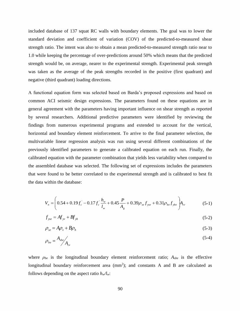
90

included database of 137 squat RC walls with boundary elements. The goal was to lower the

standard deviation and coefficient of variation (COV) of the predicted-to-measured shear

strength ratio. The intent was also to obtain a mean predicted-to-measured strength ratio near to

1.0 while keeping the percentage of over-predictions around 50% which means that the predicted

strength would be, on average, nearer to the experimental strength. Experimental peak strength

was taken as the average of the peak strengths recorded in the positive (first quadrant) and

negative (third quadrant) loading directions.

A functional equation form was selected based on Barda’s proposed expressions and based on

common ACI seismic design expressions. The parameters found on these equations are in

general agreement with the parameters having important influence on shear strength as reported

by several researchers. Additional predictive parameters were identified by reviewing the

findings from numerous experimental programs and extended to account for the vertical,

horizontal and boundary element reinforcement. To arrive to the final parameter selection, the

multivariable linear regression analysis was run using several different combinations of the

previously identified parameters to generate a calibrated equation on each run. Finally, the

calibrated equation with the parameter combination that yields less variability when compared to

the assembled database was selected. The following set of expressions includes the parameters

that were found to be better correlated to the experimental strength and is calibrated to best fit

the data within the database:

cvybebeysese

gw

w

ccn AffA

P

l

hffV

31.039.045.017.019.054.0 '' (5-1)

yhyvyse BfAff (5-2)

hvse BA (5-3)

cv

sbebe A

A

(5-4)

where ρbe is the longitudinal boundary element reinforcement ratio; Asbe is the effective

longitudinal boundary reinforcement area (mm2); and constants A and B are calculated as

follows depending on the aspect ratio hw/lw:

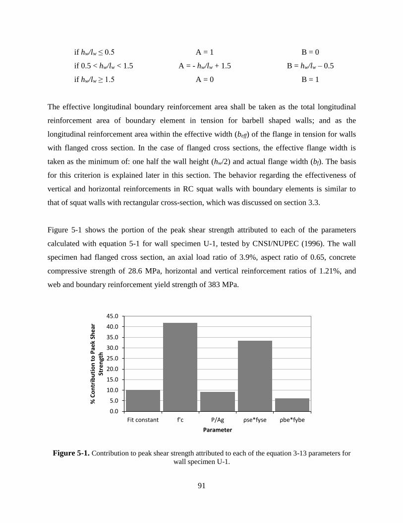
91

if hw/lw ≤ 0.5 A = 1 B = 0


if hw/lw ≥ 1.5 A = 0 B = 1

The effective longitudinal boundary reinforcement area shall be taken as the total longitudinal

reinforcement area of boundary element in tension for barbell shaped walls; and as the

longitudinal reinforcement area within the effective width (beff) of the flange in tension for walls

with flanged cross section. In the case of flanged cross sections, the effective flange width is

taken as the minimum of: one half the wall height (hw/2) and actual flange width (bf). The basis

for this criterion is explained later in this section. The behavior regarding the effectiveness of

vertical and horizontal reinforcements in RC squat walls with boundary elements is similar to

that of squat walls with rectangular cross-section, which was discussed on section 3.3.

Figure 5-1 shows the portion of the peak shear strength attributed to each of the parameters

calculated with equation 5-1 for wall specimen U-1, tested by CNSI/NUPEC (1996). The wall

specimen had flanged cross section, an axial load ratio of 3.9%, aspect ratio of 0.65, concrete

compressive strength of 28.6 MPa, horizontal and vertical reinforcement ratios of 1.21%, and

web and boundary reinforcement yield strength of 383 MPa.

Figure 5-1. Contribution to peak shear strength attributed to each of the equation 3-13 parameters for

wall specimen U-1.

0.0

5.0

10.0

15.0

20.0

25.0

30.0

35.0

40.0

45.0

Fit constant f'c P/Ag ρse*fyse ρbe*fybe

% C

on

trib

uti

on

to

Pae

k Sh

ear

St

ren

gth

Parameter

92

Other failure modes yielding lower strength can occur. The occurrence of such failure modes

may be related to differences between the actual conditions of the wall being evaluated and the

experimental setup of walls considered in the database. The user should be aware of the

characteristics and range of parameters of the wall specimens considered in the corresponding

database to determine applicability of the predictive equation.

In the same manner as for the rectangular squat walls, the parameter associated with the strength

provided by the reinforcement was evaluated by one-at-a-time parameter variation. The use of

vertical distributed reinforcement only, total vertical reinforcement (including boundary element

reinforcement) only, horizontal reinforcement only, both horizontal and vertical distributed

reinforcements in separate terms, and an effective reinforcement ratio that combines both

distributed reinforcements in one term (in the same fashion as in ASCE 43-05) were considered.

The last resulted to be a better predictive parameter for steel contribution to shear strength as it

produced the least variability. Using the effective reinforcement ratio to consider the contribution

of both steel reinforcements as a function of aspect ratio seems to be a reasonable assumption

and is in good general agreement with experimental findings (Figure 3-2).

It has been consistently reported by researchers that walls with lower aspect ratios or lower shear

span-to-length ratios can yield higher shear stress capacities. This has been commonly attributed

to an increase in the shear carried by concrete as the aspect ratio decreases. In a preliminary

study (Adorno-Bonilla and Vidot-Vega, 2015), the aspect ratio was treated as a separate term and

compared to equation calibration using a term that considers the product of a concrete strength

parameter and the aspect ratio. It was found that using the product of aspect ratio and a concrete

strength parameter produced better predictions than using the aspect ratio separately. Additional

to the term considering the product of aspect ratio and concrete strength, the use of another term

with concrete strength parameter only was also considered, which further improved the

predictions. Different combinations using the aspect ratio and the shear span-to-length ratio were

evaluated. Also, the use of the square root of the concrete compressive strength (√𝑓𝑐′) versus

using the compressive strength itself (f’c) was considered.

The aspect ratio (hw/lw) was found to produce better correlation with the included database (with

cantilever test setup) than the shear span (M/Vlw). The aspect ratio is a more practical parameter

93

for design purposes, since it does not depend on structural analysis to calculate values for

moment and shear. However, if a wall pier with both ends fixed is being considered, then the use

of the M/Vlw would be more appropriate. The concrete compressive strength (f’c) resulted to be a

better strength prediction parameter; with best results when a concrete strength term and another

term with the product of concrete strength and wall aspect ratio were included in the equation.

The boundary element reinforcement ratio is not considered in most currently available

equations. However, several researchers (e.g., Endo, 1980; Wood, 1990; and Terzioğlu, 2011)

have found that the boundary element reinforcement affects both the shear load transfer

mechanism and the peak shear strength even in shear-dominated walls with very low aspect

ratios. Therefore, a term with the longitudinal boundary element reinforcement ratio (ρbe),

calculated as the ratio of longitudinal boundary reinforcement area in tension to the effective

shear area (Asbe/Acv), was included resulting in an enhancement in prediction performance.

Another option where the ρbe was calculated as the ratio of longitudinal boundary reinforcement

area in tension to the gross area of the corresponding boundary element (Asbe/Abe) was evaluated

as well, but better predictions were obtained using Asbe/Acv.

This group of walls is comprised of barbell and flange cross sections which, in general, can reach

higher shear stresses than those of rectangular cross section. Specifically, the walls with flanged

cross section can have a shear lag effect which makes the tensile steel stresses to be non-uniform

along the flange width. These stresses are higher at the center of the flange width (nearer to the

web), and decrease with increasing distance from the web in the outward direction as shown in

Figure 5-2. Therefore, if we consider all the steel within the whole flange width to be effective,

we might be using an unrealistic assumption especially for the case of walls with wide flanges.

A typical approach used in design codes and standards, is to assume an effective flange width

where the steel is fully effective. In order to address this effect, and to obtain a more accurate

predictive equation, different criteria found in standards and in literature for determining the

effective flange width were considered. Then, the boundary element reinforcement ratios were

calculated for each case and the equations were fitted by multiple linear regression against the

data of walls with flanged cross section. This allowed determining which assumption of the

effective flange width would give a better predictive performance by comparing the variability of

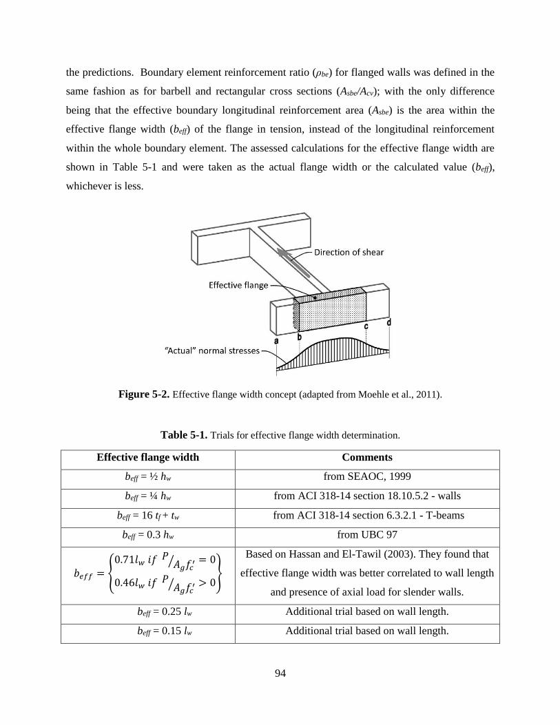
94

the predictions. Boundary element reinforcement ratio (ρbe) for flanged walls was defined in the

same fashion as for barbell and rectangular cross sections (Asbe/Acv); with the only difference

being that the effective boundary longitudinal reinforcement area (Asbe) is the area within the

effective flange width (beff) of the flange in tension, instead of the longitudinal reinforcement

within the whole boundary element. The assessed calculations for the effective flange width are

shown in Table 5-1 and were taken as the actual flange width or the calculated value (beff),

whichever is less.

Figure 5-2. Effective flange width concept (adapted from Moehle et al., 2011).

Table 5-1. Trials for effective flange width determination.

Effective flange width Comments

beff = ½ hw from SEAOC, 1999

beff = ¼ hw from ACI 318-14 section 18.10.5.2 - walls

beff = 16 tf + tw from ACI 318-14 section 6.3.2.1 - T-beams

beff = 0.3 hw from UBC 97

𝑏𝑒𝑓𝑓 = {0.71𝑙𝑤 𝑖𝑓 𝑃

𝐴𝑔𝑓𝑐′⁄ = 0

0.46𝑙𝑤 𝑖𝑓 𝑃𝐴𝑔𝑓𝑐

′⁄ > 0}

Based on Hassan and El-Tawil (2003). They found that

effective flange width was better correlated to wall length

and presence of axial load for slender walls.

beff = 0.25 lw Additional trial based on wall length.

beff = 0.15 lw Additional trial based on wall length.

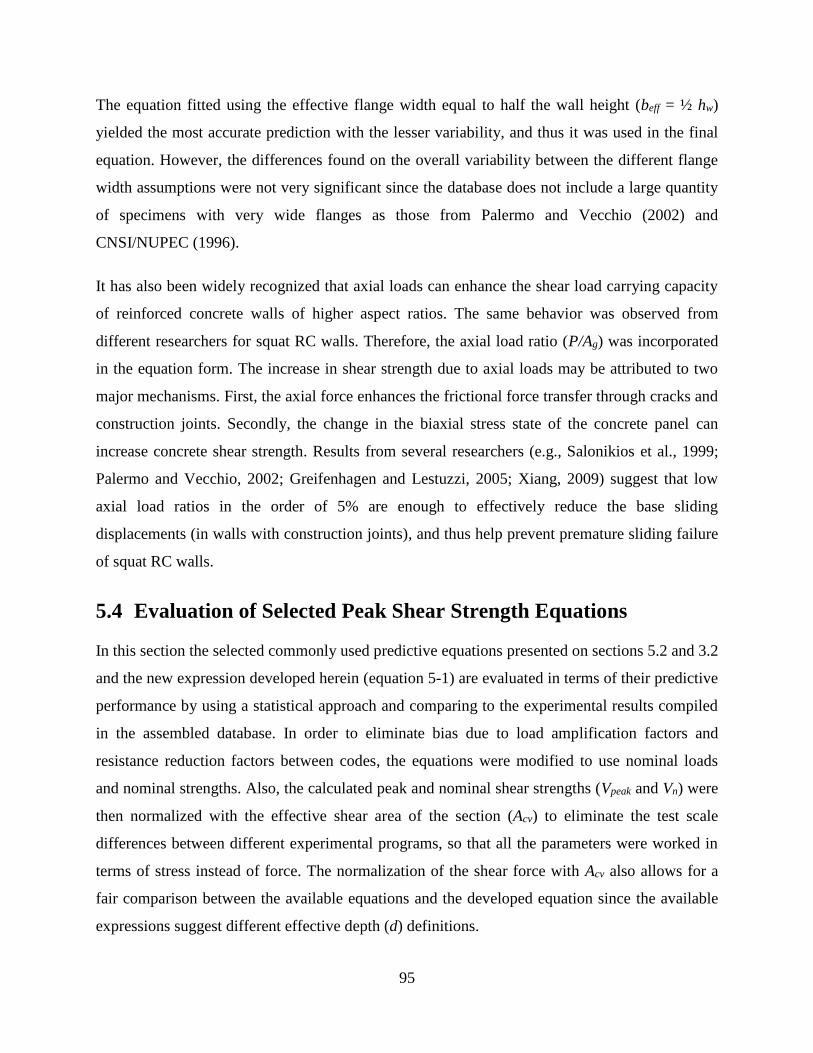
95

The equation fitted using the effective flange width equal to half the wall height (beff = ½ hw)

yielded the most accurate prediction with the lesser variability, and thus it was used in the final

equation. However, the differences found on the overall variability between the different flange

width assumptions were not very significant since the database does not include a large quantity

of specimens with very wide flanges as those from Palermo and Vecchio (2002) and

CNSI/NUPEC (1996).

It has also been widely recognized that axial loads can enhance the shear load carrying capacity

of reinforced concrete walls of higher aspect ratios. The same behavior was observed from

different researchers for squat RC walls. Therefore, the axial load ratio (P/Ag) was incorporated

in the equation form. The increase in shear strength due to axial loads may be attributed to two

major mechanisms. First, the axial force enhances the frictional force transfer through cracks and

construction joints. Secondly, the change in the biaxial stress state of the concrete panel can

increase concrete shear strength. Results from several researchers (e.g., Salonikios et al., 1999;

Palermo and Vecchio, 2002; Greifenhagen and Lestuzzi, 2005; Xiang, 2009) suggest that low

axial load ratios in the order of 5% are enough to effectively reduce the base sliding

displacements (in walls with construction joints), and thus help prevent premature sliding failure

of squat RC walls.

5.4 Evaluation of Selected Peak Shear Strength Equations

In this section the selected commonly used predictive equations presented on sections 5.2 and 3.2

and the new expression developed herein (equation 5-1) are evaluated in terms of their predictive

performance by using a statistical approach and comparing to the experimental results compiled

in the assembled database. In order to eliminate bias due to load amplification factors and

resistance reduction factors between codes, the equations were modified to use nominal loads

and nominal strengths. Also, the calculated peak and nominal shear strengths (Vpeak and Vn) were

then normalized with the effective shear area of the section (Acv) to eliminate the test scale

differences between different experimental programs, so that all the parameters were worked in

terms of stress instead of force. The normalization of the shear force with Acv also allows for a

fair comparison between the available equations and the developed equation since the available

expressions suggest different effective depth (d) definitions.

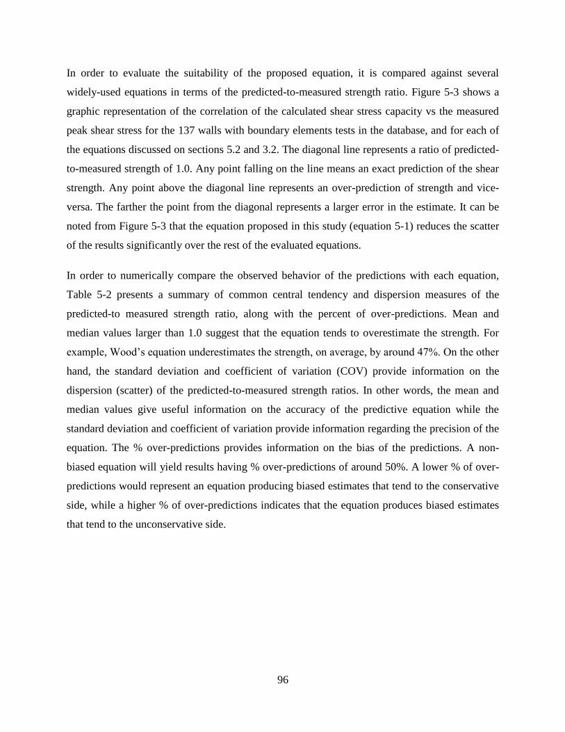
96

In order to evaluate the suitability of the proposed equation, it is compared against several

widely-used equations in terms of the predicted-to-measured strength ratio. Figure 5-3 shows a

graphic representation of the correlation of the calculated shear stress capacity vs the measured

peak shear stress for the 137 walls with boundary elements tests in the database, and for each of

the equations discussed on sections 5.2 and 3.2. The diagonal line represents a ratio of predicted-

to-measured strength of 1.0. Any point falling on the line means an exact prediction of the shear

strength. Any point above the diagonal line represents an over-prediction of strength and vice-

versa. The farther the point from the diagonal represents a larger error in the estimate. It can be

noted from Figure 5-3 that the equation proposed in this study (equation 5-1) reduces the scatter

of the results significantly over the rest of the evaluated equations.

In order to numerically compare the observed behavior of the predictions with each equation,


predicted-to measured strength ratio, along with the percent of over-predictions. Mean and

median values larger than 1.0 suggest that the equation tends to overestimate the strength. For

example, Wood’s equation underestimates the strength, on average, by around 47%. On the other

hand, the standard deviation and coefficient of variation (COV) provide information on the

dispersion (scatter) of the predicted-to-measured strength ratios. In other words, the mean and

median values give useful information on the accuracy of the predictive equation while the

standard deviation and coefficient of variation provide information regarding the precision of the

equation. The % over-predictions provides information on the bias of the predictions. A non-

biased equation will yield results having % over-predictions of around 50%. A lower % of over-

predictions would represent an equation producing biased estimates that tend to the conservative

side, while a higher % of over-predictions indicates that the equation produces biased estimates

that tend to the unconservative side.

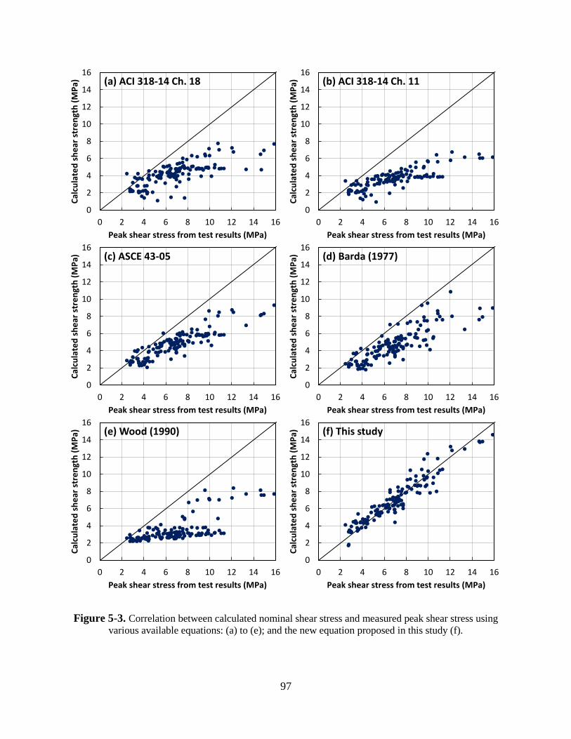
97

Figure 5-3. Correlation between calculated nominal shear stress and measured peak shear stress using


0

2

4

6

8

10

12

14

16

0 2 4 6 8 10 12 14 16

Cal

cula

ted

sh

ear

str

en

gth

(M

Pa)


(a) ACI 318-14 Ch. 18

0

2

4

6

8

10

12

14

16

0 2 4 6 8 10 12 14 16

Cal

cula

ted

sh

ear

str

en

gth

(M

Pa)


(b) ACI 318-14 Ch. 11

0

2

4

6

8

10

12

14

16

0 2 4 6 8 10 12 14 16

Cal

cula

ted

sh

ear

str

en

gth

(M

Pa)


(c) ASCE 43-05

0

2

4

6

8

10

12

14

16

0 2 4 6 8 10 12 14 16

Cal

cula

ted

sh

ear

str

en

gth

(M

Pa)


(d) Barda (1977)

0

2

4

6

8

10

12

14

16

0 2 4 6 8 10 12 14 16

Cal

cula

ted

sh

ear

str

en

gth

(M

Pa)


(e) Wood (1990)

0

2

4

6

8

10

12

14

16

0 2 4 6 8 10 12 14 16

Cal

cula

ted

sh

ear

str

en

gth

(M

Pa)


(f) This study

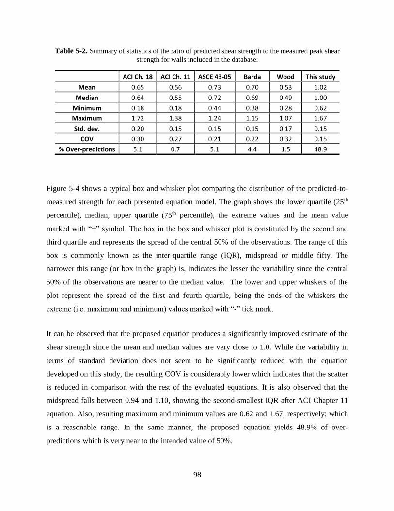
98

Table 5-2. Summary of statistics of the ratio of predicted shear strength to the measured peak shear

strength for walls included in the database.


Mean 0.65 0.56 0.73 0.70 0.53 1.02

Median 0.64 0.55 0.72 0.69 0.49 1.00

Minimum 0.18 0.18 0.44 0.38 0.28 0.62

Maximum 1.72 1.38 1.24 1.15 1.07 1.67

Std. dev. 0.20 0.15 0.15 0.15 0.17 0.15

COV 0.30 0.27 0.21 0.22 0.32 0.15



measured strength for each presented equation model. The graph shows the lower quartile (25th

percentile), median, upper quartile (75th percentile), the extreme values and the mean value

marked with “+” symbol. The box in the box and whisker plot is constituted by the second and

third quartile and represents the spread of the central 50% of the observations. The range of this

box is commonly known as the inter-quartile range (IQR), midspread or middle fifty. The

narrower this range (or box in the graph) is, indicates the lesser the variability since the central

50% of the observations are nearer to the median value. The lower and upper whiskers of the

plot represent the spread of the first and fourth quartile, being the ends of the whiskers the

extreme (i.e. maximum and minimum) values marked with “-” tick mark.

It can be observed that the proposed equation produces a significantly improved estimate of the

shear strength since the mean and median values are very close to 1.0. While the variability in

terms of standard deviation does not seem to be significantly reduced with the equation

developed on this study, the resulting COV is considerably lower which indicates that the scatter

is reduced in comparison with the rest of the evaluated equations. It is also observed that the

midspread falls between 0.94 and 1.10, showing the second-smallest IQR after ACI Chapter 11

equation. Also, resulting maximum and minimum values are 0.62 and 1.67, respectively; which

is a reasonable range. In the same manner, the proposed equation yields 48.9% of over-

predictions which is very near to the intended value of 50%.

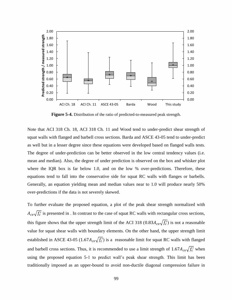
99

Figure 5-4. Distribution of the ratio of predicted-to-measured peak strength.

Note that ACI 318 Ch. 18, ACI 318 Ch. 11 and Wood tend to under-predict shear strength of

squat walls with flanged and barbell cross sections. Barda and ASCE 43-05 tend to under-predict

as well but in a lesser degree since these equations were developed based on flanged walls tests.

The degree of under-prediction can be better observed in the low central tendency values (i.e.

mean and median). Also, the degree of under prediction is observed on the box and whisker plot

where the IQR box is far below 1.0, and on the low % over-predictions. Therefore, these

equations tend to fall into the conservative side for squat RC walls with flanges or barbells.

Generally, an equation yielding mean and median values near to 1.0 will produce nearly 50%

over-predictions if the data is not severely skewed.

To further evaluate the proposed equation, a plot of the peak shear strength normalized with

𝐴𝑐𝑣√𝑓𝑐′ is presented in . In contrast to the case of squat RC walls with rectangular cross sections,

this figure shows that the upper strength limit of the ACI 318 (0.83𝐴𝑐𝑣√𝑓𝑐′) is not a reasonable

value for squat shear walls with boundary elements. On the other hand, the upper strength limit

established in ASCE 43-05 (1.67𝐴𝑐𝑣√𝑓𝑐′) is a reasonable limit for squat RC walls with flanged

and barbell cross sections. Thus, it is recommended to use a limit strength of 1.67𝐴𝑐𝑣√𝑓𝑐′ when

using the proposed equation 5-1 to predict wall’s peak shear strength. This limit has been

traditionally imposed as an upper-bound to avoid non-ductile diagonal compression failure in

0.00

0.20

0.40

0.60

0.80

1.00

1.20

1.40

1.60

1.80

2.00

0.00

0.20

0.40

0.60

0.80

1.00

1.20

1.40

1.60

1.80

2.00


Pre

dic

ted

str

en

gth

/ m

eas

ure

d s

tre

ngt

h

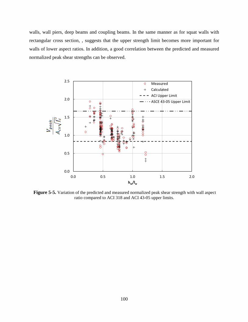
100

walls, wall piers, deep beams and coupling beams. In the same manner as for squat walls with

rectangular cross section, , suggests that the upper strength limit becomes more important for

walls of lower aspect ratios. In addition, a good correlation between the predicted and measured

normalized peak shear strengths can be observed.

Figure 5-5. Variation of the predicted and measured normalized peak shear strength with wall aspect

ratio compared to ACI 318 and ACI 43-05 upper limits.

0.0

0.5

1.0

1.5

2.0

2.5

0.0 0.5 1.0 1.5 2.0

hw/lw

Measured

Calculated

ACI Upper Limit

ASCE 43-05 Upper Limit

101

DISPLACEMENT CAPACITY OF SQUAT

WALLS WITH BOUNDARY ELEMENTS

6.1 Introduction

It was noted on Chapters 3 and 5 that squat RC walls with enlarged boundary elements can show

different behavior than those with rectangular cross section. This difference was mainly observed

in the strength but, in order to maintain uniformity, the assessment of available predictive

equations and development of new predictive equations was addressed separately for both groups

of walls.

This chapter presents an evaluation of current expressions for the prediction of the displacement

capacity of squat reinforced concrete walls with enlarged boundary elements (i.e. flanged and

barbell-shaped cross section) found in the literature. The performance of each of the selected

equations was assessed by comparing the displacement predictions with experimental

displacements from the assembled database for walls with enlarged boundary elements. Key

parameters influencing the displacement capacity were identified. The experimental

displacements of each wall were taken as the average of the displacements measured from the

first and third quadrants (i.e. positive and negative loading directions, respectively). New

equations to predict the cracking, peak, and ultimate displacement capacities of squat walls with

boundary elements are presented to improve current displacement estimates. These displacement

capacity estimates, in conjunction with the peak strength estimate presented in Chapter 5 can be

used to define the backbone curve for a hysteretic model. The equations were obtained from

multivariable linear regression analyses using an assembled experimental database from various

experimental programs which is presented on Chapter 2 and Appendix A. The expressions

presented herein were intended to apply for squat walls with rectangular cross section and a wide

range of characteristics.

6.2 Current Expressions for Estimation of Displacement Capacity

The selected predictive equations for displacement capacity were found in US standards and in

literature. The models proposed by Hidalgo et al. (2000), Carrillo (2010), Sánchez (2013), Gérin

102

and Adebar (2004) and ASCE 41-13 were considered. A brief introduction to these models is

given in this section and section 4.2 presents a detailed discussion of the selected current

equations for displacement capacity prediction.

Hidalgo et al. (2000) developed a hysteretic model for the analysis of cyclic lateral load-

displacement behavior of squat RC shear walls. The authors used a tri-linear hysteresis envelope

and proposed equations 4-1 to 4-6 for the estimation of the drift at shear cracking, peak strength,

and the ultimate drift based on linear regression from experimental results. The authors

recommended using a modified version of ACI 318 seismic design provisions for determining

the peak shear strength. The shear force corresponding to the cracking point was recommended

to be taken as the calculated concrete contribution to strength. The ultimate displacement was

defined as that associated to a 20% drop in strength (80% Vpeak) past the peak point.

Carrillo (2010) presented a tri-linear backbone model for the analysis of squat walls. The model

was based on the observations from experimental tests representative of typical squat RC walls

of housing construction in several Latin American countries. In the same manner as in the model

by Hidalgo et al. (2000), the model presented by Carrillo (2010) has a tri-linear backbone with a

stiffness reduction point associated to significant diagonal web cracking. Carrillo (2010)

proposed equations 4-7 to 4-10 equations to calculate the drift ratio at diagonal cracking, peak

strength and ultimate state as a percentage. Ultimate displacement was defined as the

displacement associated to a 20% decrease in strength (80% Vpeak) after peak point. The cracking

strength was assumed as the concrete contribution to shear strength.

Sánchez (2013) proposed a backbone model similar to that proposed by Hidalgo et al. (2000) and

Carrillo (2010), but modified to include a first stiffness reduction due to flexural cracking and a

second stiffness reduction due to distributed diagonal cracking. An additional line segment to

represent the initial uncracked stiffness and the reduced stiffness after flexural cracking was

included. Based on the experimental results from RC shear walls with similar characteristics of

those used for housing construction in Mexico, Sánchez (2013) proposed equations 4-11 to 4-18

to estimate the points of the backbone curve corresponding to flexural cracking, diagonal

cracking, peak strength and ultimate damage state. The author proposed to estimate the

displacement at peak strength (Δpeak) by adding the flexural (Δf) and shear (Δs) displacement

103

components and proposed separate equations for their calculation. Sánchez (2013) used the same

20% strength degradation criterion to define the ultimate damage state as used by other

researchers. Sánchez (2013) used a ductility-based approach to calibrate the expressions for

estimation of the ultimate displacement (Δu).

Gérin and Adebar (2004) proposed a model to calculate the load-displacement response of

reinforced concrete elements controlled by brittle shear failure under reversed cyclic shear

loading. The model was based on theoretical mechanics and the experimental observations of 21

large-scale membrane-type element tests. The backbone curve shows major stiffness degradation

due to diagonal cracking and a yield plateau after attaining peak strength. Equations 4-19 to 4-

24 were proposed by Gérin and Adebar (2004) to calculate the backbone points corresponding to

diagonal cracking, yield (peak strength) and ultimate damage state. On this model, the yield

(peak) stress (vy) is recommended to be calculated per seismic provisions of ACI 318-08. The

model assumes that shear yielding is associated to the yield of reinforcement. A ductility

expression calibrated with experimental data was proposed to obtain ultimate shear strain (γu);

associated to a concrete shear failure due to large displacements along cracks. A conservative

limit in the shear ductility was imposed to consider the possibility of concrete diagonal

compression failure which could occur in walls with high reinforcement ratios.

ASCE 41-06 standard has been updated to ASCE 41-13 which now incorporates a major

stiffness reduction prior to peak strength in the backbone curve to consider the effect of typical

inclined shear cracking and provide a better representation of low-rise walls behavior. The

changes are based on recommendations by Wallace (2007). Shear cracking is assumed to occur

at the development of 60% of the peak strength and the corresponding displacement is calculated

using the elastic stiffness of a cantilever wall considering flexural and shear deformations and

uncracked properties. Shear strength is calculated using ACI 318 seismic provisions. The model

provides fixed drift ratio values for the drift capacity. In order to consider the effects of axial

load, the model reduces the drift capacity from 1% to 0.75% and the residual strength from

0.2Vpeak to 0 for walls with axial load ratios (P/f’cAg) greater than 0.05.

Duffey et al. (1994a, 1994b) suggested average values for drift ratio at peak strength and at

several post-peak strength degradation stages, based on statistical analysis of experimental data

104

compiled from numerous experimental studies. Due to the typical brittle response of squat RC

walls, and the lack of sufficient experimental data of post-peak response, the authors

recommended using the drift ratio values associated to the peak strength as the ultimate drift

capacity when performing analyses using hysteretic models. Duffey et al. (1994a, 1994b) also

noted that the allowable drift limits on most design codes and standards tend to be

unconservative for low-rise RC shear walls since those are mainly focused on high rise buildings

comprised of slender walls, which generally have higher ductility.

6.3 Development of New Displacement Capacity Predictive

Equations

As discussed on section 4.3 the lateral load-displacement envelopes of squat RC walls can be

adequately represented by a tri-linear backbone as shown in Figure 4-1. Therefore, drift data was

collected from numerous experiments found in literature and were included in the assembled

database for the three main points defining the tri-linear backbone (i.e. significant diagonal

cracking, peak strength, and ultimate damage state). The availability of displacement data is

more limited than peak strength data since no drift data was reported on some of the evaluated

references, while for some other tests only data of drift at peak strength was available. From the

137 wall specimens with enlarged boundary elements (barbell and flanged cross section) listed in

the database, drift data collection was possible for 67 and 82 specimens for the cracking and

peak points, respectively. The drift data for the ultimate damage state was even scarcer since

many of the early experimental studies presented data only up to the peak strength. Therefore,

only 59 qualifying datasets could be obtained from the evaluated references for ultimate drift of

walls with enlarged boundary elements.

In the same manner as for the walls with rectangular cross section, most of the data was obtained

from global force-displacement hysteresis curves, including the contribution of both shear and

flexural deformations, found on the evaluated references. The vast majority of cyclic loading

tests were displacement controlled, typically with two or three cycles at each displacement level

as shown on Figure 4-5. The drift data was obtained from the experimental envelopes which

were extracted by tracing straight lines connecting all the first cycle peaks of the hysteresis loops

(see Figure 4-5). The load-displacement envelope was not extrapolated beyond the last loading

105

peaks. The data was converted to drift ratio to make all the measurements comparable.

Afterwards, the drift ratios corresponding to the assumed diagonal cracking condition (Rcr), peak

strength (Rpeak) and ultimate state (Ru) were retrieved from the obtained cyclic envelope. The

average drift ratio from 1st and 3rd quadrants of each wall was recorded for each of the three

states. Cracking drift ratio was defined as that corresponding to the development of 60% of peak

strength, while ultimate drift ratio was defined as that corresponding to the post-peak point

where a strength degradation of 20% is attained. For tests where ultimate displacement data was

not available for one of the loading directions (commonly when test is stopped due to sudden

failure in the opposite direction), the single value available for the ultimate displacement was

recorded. Further details are discussed in the next sub-sections and in Chapter 4.

The same methodology used in Chapter 4 for the walls with rectangular cross sections is used in

this chapter for the walls with enlarged boundary elements. Regression analyses were performed

to develop empirical equations that better fits the collected drift data. The goal was to lower the

coefficient of variation and to obtain a mean value near to 1.0 for the ratio of predicted-to-

measured drift capacity. Key parameters were identified by evaluating the correlation coefficient

with the drift capacity. Multivariable linear regression analyses were carried to derive the

equations with the selected parameters. An iterative process of eliminating the least meaningful

parameter based on the highest p-value, and re-calibration until the scatter of the prediction was

observed to increase, was used to simplify the equations. In order to minimize bias due to test

specimens’ scale, the collected displacement data was converted to drift ratio, reinforcement

spacing was normalized with wall thickness and any parameter involving forces was normalized

with the effective shear area of the cross section (Acv) for the calibration and development of

equations. The following sub-sections present the simplified expressions using the most

significant parameters that were found to produce a better correlation with the barbell/flanged

walls database, and are proposed for the prediction of drift ratio at diagonal cracking, drift ratio

at peak strength and at ultimate drift ratio, respectively.


As previously discussed, it was considered that the main stiffness reduction on the load-

displacement envelope of squat RC shear walls is related to the development of significant

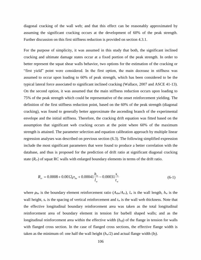
106

diagonal cracking of the wall web; and that this effect can be reasonably approximated by

assuming the significant cracking occurs at the development of 60% of the peak strength.

Further discussion on this first stiffness reduction is provided on section 4.3.1.

For the purpose of simplicity, it was assumed in this study that both, the significant inclined

cracking and ultimate damage states occur at a fixed portion of the peak strength. In order to

better represent the squat shear walls behavior, two options for the estimation of the cracking or

“first yield” point were considered. In the first option, the main decrease in stiffness was

assumed to occur upon loading to 60% of peak strength, which has been considered to be the

typical lateral force associated to significant inclined cracking (Wallace, 2007 and ASCE 41-13).

On the second option, it was assumed that the main stiffness reduction occurs upon loading to

75% of the peak strength which could be representative of the onset reinforcement yielding. The

definition of the first stiffness reduction point, based on the 60% of the peak strength (diagonal

cracking), was found to generally better approximate the ascending branch of the experimental

envelope and the initial stiffness. Therefore, the cracking drift equation was fitted based on the

assumption that significant web cracking occurs at the point where 60% of the maximum

strength is attained. The parameter selection and equation calibration approach by multiple linear

regression analyses was described on previous section (6.3). The following simplified expression

include the most significant parameters that were found to produce a better correlation with the

database, and thus is proposed for the prediction of drift ratio at significant diagonal cracking

state (Rcr) of squat RC walls with enlarged boundary elements in terms of the drift ratio.

where ρbe is the boundary element reinforcement ratio (Asbe/Acv), lw is the wall length, hw is the

wall height, sv is the spacing of vertical reinforcement and tw is the wall web thickness. Note that

the effective longitudinal boundary reinforcement area was taken as the total longitudinal

reinforcement area of boundary element in tension for barbell shaped walls; and as the

longitudinal reinforcement area within the effective width (beff) of the flange in tension for walls

with flanged cross section. In the case of flanged cross sections, the effective flange width is

taken as the minimum of: one half the wall height (hw/2) and actual flange width (bf).

w

v

w

w

becrt

s

l

hR 00031.000041.00012.00008.0 (6-1)

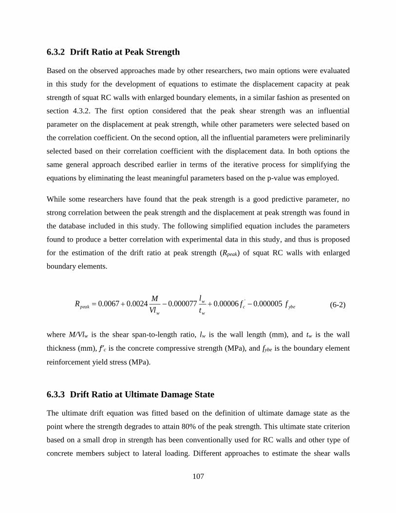
107


Based on the observed approaches made by other researchers, two main options were evaluated

in this study for the development of equations to estimate the displacement capacity at peak

strength of squat RC walls with enlarged boundary elements, in a similar fashion as presented on

section 4.3.2. The first option considered that the peak shear strength was an influential

parameter on the displacement at peak strength, while other parameters were selected based on

the correlation coefficient. On the second option, all the influential parameters were preliminarily

selected based on their correlation coefficient with the displacement data. In both options the

same general approach described earlier in terms of the iterative process for simplifying the

equations by eliminating the least meaningful parameters based on the p-value was employed.

While some researchers have found that the peak strength is a good predictive parameter, no

strong correlation between the peak strength and the displacement at peak strength was found in

the database included in this study. The following simplified equation includes the parameters

found to produce a better correlation with experimental data in this study, and thus is proposed

for the estimation of the drift ratio at peak strength (Rpeak) of squat RC walls with enlarged

boundary elements.

where M/Vlw is the shear span-to-length ratio, lw is the wall length (mm), and tw is the wall

thickness (mm), f’c is the concrete compressive strength (MPa), and fybe is the boundary element

reinforcement yield stress (MPa).


The ultimate drift equation was fitted based on the definition of ultimate damage state as the

point where the strength degrades to attain 80% of the peak strength. This ultimate state criterion

based on a small drop in strength has been conventionally used for RC walls and other type of

concrete members subject to lateral loading. Different approaches to estimate the shear walls

ybec

w

w

w

peak fft

l

Vl

MR 000005.000006.0000077.00024.00067.0 ' (6-2)

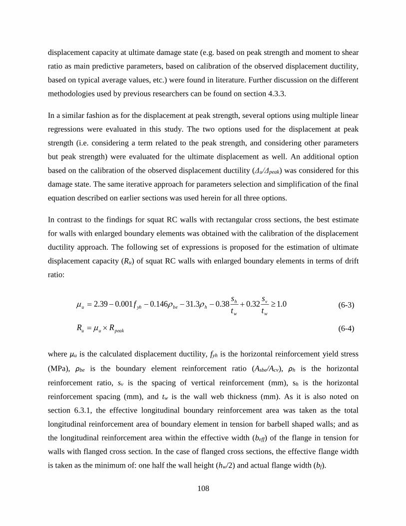
108

displacement capacity at ultimate damage state (e.g. based on peak strength and moment to shear

ratio as main predictive parameters, based on calibration of the observed displacement ductility,

based on typical average values, etc.) were found in literature. Further discussion on the different

methodologies used by previous researchers can be found on section 4.3.3.

In a similar fashion as for the displacement at peak strength, several options using multiple linear

regressions were evaluated in this study. The two options used for the displacement at peak

strength (i.e. considering a term related to the peak strength, and considering other parameters

but peak strength) were evaluated for the ultimate displacement as well. An additional option

based on the calibration of the observed displacement ductility (Δu/Δpeak) was considered for this

damage state. The same iterative approach for parameters selection and simplification of the final

equation described on earlier sections was used herein for all three options.

In contrast to the findings for squat RC walls with rectangular cross sections, the best estimate

for walls with enlarged boundary elements was obtained with the calibration of the displacement

ductility approach. The following set of expressions is proposed for the estimation of ultimate

displacement capacity (Ru) of squat RC walls with enlarged boundary elements in terms of drift

ratio:

where μu is the calculated displacement ductility, fyh is the horizontal reinforcement yield stress

(MPa), ρbe is the boundary element reinforcement ratio (Asbe/Acv), ρh is the horizontal

reinforcement ratio, sv is the spacing of vertical reinforcement (mm), sh is the horizontal

reinforcement spacing (mm), and tw is the wall web thickness (mm). As it is also noted on

section 6.3.1, the effective longitudinal boundary reinforcement area was taken as the total

longitudinal reinforcement area of boundary element in tension for barbell shaped walls; and as

the longitudinal reinforcement area within the effective width (beff) of the flange in tension for

walls with flanged cross section. In the case of flanged cross sections, the effective flange width

is taken as the minimum of: one half the wall height (hw/2) and actual flange width (bf).

0.132.038.03.31146.0001.039.2 w

v

w

h

hbeyhut

s

t

sf (6-3)

peakuu RR (6-4)

109

6.4 Evaluation of Selected Displacement Capacity Equations

In this section the selected predictive equations found in literature and the new expressions

developed herein are evaluated in terms of their predictive performance by using a statistical

analysis approach and comparing to the experimental data compiled in the assembled database

(Appendix A). In order to minimize bias due to test specimens scale, all the displacement

predictions were converted to drift ratio for comparison.

The following subsections show detailed analysis of the performance of each of the equations

developed in this study for the prediction of displacement capacity of squat RC walls with

enlarged boundary elements, at each of the three defined damage states, and compared to the

performance of the corresponding equations found in literature. Tabulated summaries of

common central tendency and dispersion measures of the predicted-to-measured drift ratios,

along with the percent of over-predictions are presented in the same fashion as presented on

Chapter 4 for the prediction of displacement capacity of squat RC walls with rectangular cross

sections. Mean and median values larger than 1.0 suggest that the equation tends to overestimate

the drift ratio. Standard deviation and coefficient of variation (COV) provide information on the

dispersion (scatter) of the predicted-to-measured drift ratio, where lower values mean less

variability. The % over-predictions provides information on the bias of the predictions where a

non-biased equation will yield around 50% over-predictions. A lower % of over-predictions

would represent an equation producing biased estimates that tend to underestimate drift ratios,

while a higher % of over-predictions indicates that the equation produces biased estimates that

tend to overestimate drift ratios.

Sections 6.4.1, 6.4.2 and 6.4.3 will discuss the findings for the displacement at diagonal

cracking, displacement at peak strength and ultimate displacement, respectively.


The performance of the equations for the prediction of the cracking or “first yield” displacement

will not be compared because all of them are based on different assumptions of the

corresponding strength at which the stiffness reduction occurs, and therefore, are not directly

comparable. Thus, only statistical analysis of the drift ratio at diagonal cracking predictions

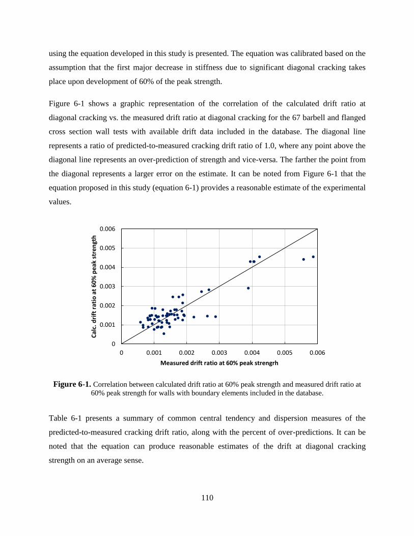
110

using the equation developed in this study is presented. The equation was calibrated based on the

assumption that the first major decrease in stiffness due to significant diagonal cracking takes

place upon development of 60% of the peak strength.

Figure 6-1 shows a graphic representation of the correlation of the calculated drift ratio at

diagonal cracking vs. the measured drift ratio at diagonal cracking for the 67 barbell and flanged

cross section wall tests with available drift data included in the database. The diagonal line

represents a ratio of predicted-to-measured cracking drift ratio of 1.0, where any point above the

diagonal line represents an over-prediction of strength and vice-versa. The farther the point from

the diagonal represents a larger error on the estimate. It can be noted from Figure 6-1 that the

equation proposed in this study (equation 6-1) provides a reasonable estimate of the experimental

values.

Figure 6-1. Correlation between calculated drift ratio at 60% peak strength and measured drift ratio at

60% peak strength for walls with boundary elements included in the database.


predicted-to-measured cracking drift ratio, along with the percent of over-predictions. It can be

noted that the equation can produce reasonable estimates of the drift at diagonal cracking

strength on an average sense.

0

0.001

0.002

0.003

0.004

0.005

0.006

0 0.001 0.002 0.003 0.004 0.005 0.006

Cal

c. d

rift

rat

io a

t 6

0%

pe

ak s

tre

ngt

h

Measured drift ratio at 60% peak strengrh

111

Table 6-1. Summary of statistics of the ratio of predicted-to-measured drift at 60% peak strength for

walls with boundary elements included in the database.

This study

Mean 1.08

Median 1.06

Minimum 0.41

Maximum 1.99

Std. dev 0.35

COV 0.32

% Over-predictions 61.2

The equation for the drift at diagonal cracking obtained for walls with enlarged boundary

elements in this section produced a better correlation with experimental data than the developed

on section 4.3.1 for walls with rectangular cross section since the mean and median values are

closer to 1.0 and yields a lower COV in terms of the ratio of predicted-to-measured cracking

drift. The % of over-predictions is slightly high which means that the backbone model would

tend to slightly underestimate the initial stiffness.



ratio at peak strength, it is compared against several equations/models found in literature. Figure

6-2 shows a graphic representation of the correlation of the calculated drift ratio at peak strength

vs. the measured drift ratio at peak strength for the 82 obtained datasets of walls with enlarged

boundary elements in the database, and for each of the equations presented on section 4.2.

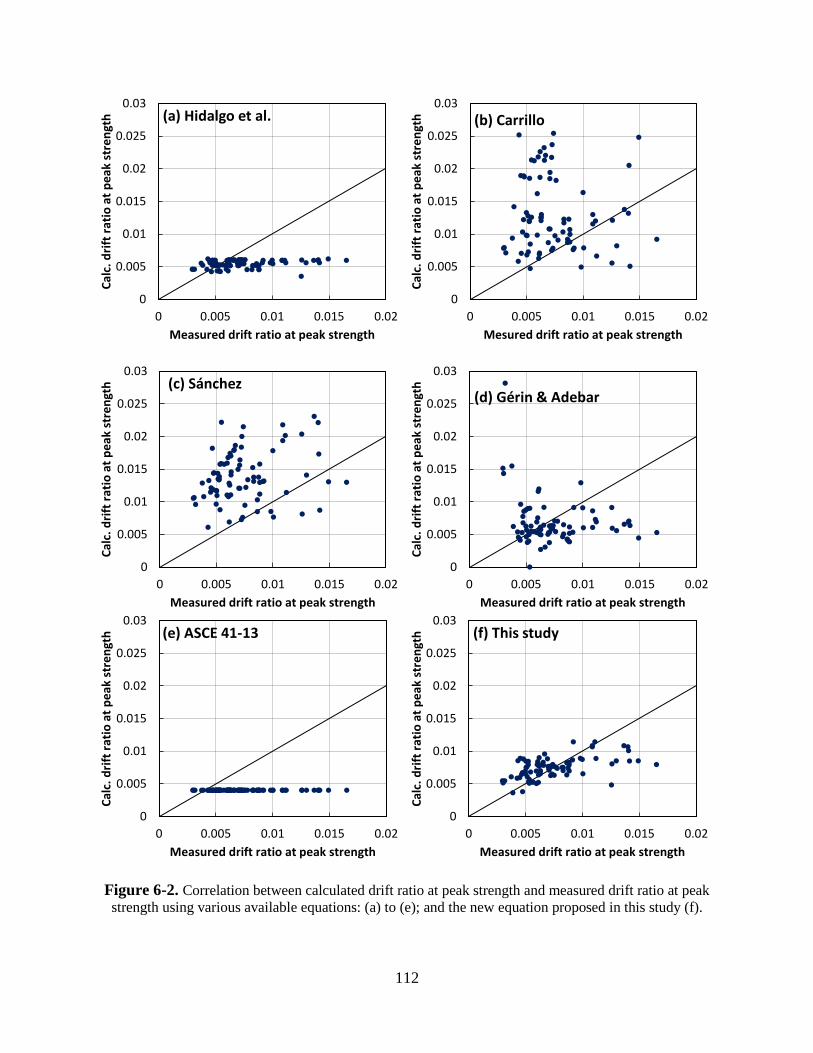
112

Figure 6-2. Correlation between calculated drift ratio at peak strength and measured drift ratio at peak

strength using various available equations: (a) to (e); and the new equation proposed in this study (f).

0

0.005

0.01

0.015

0.02

0.025

0.03

0 0.005 0.01 0.015 0.02

Cal

c. d

rift

rat

io a

t p

eak

str

en

gth


(a) Hidalgo et al.

0

0.005

0.01

0.015

0.02

0.025

0.03

0 0.005 0.01 0.015 0.02

Cal

c. d

rift

rat

io a

t p

eak

str

en

gth

Mesured drift ratio at peak strength

(b) Carrillo

0

0.005

0.01

0.015

0.02

0.025

0.03

0 0.005 0.01 0.015 0.02

Cal

c. d

rift

rat

io a

t p

eak

str

en

gth


(c) Sánchez

0

0.005

0.01

0.015

0.02

0.025

0.03

0 0.005 0.01 0.015 0.02

Cal

c. d

rift

rat

io a

t p

eak

str

en

gth


(d) Gérin & Adebar

0

0.005

0.01

0.015

0.02

0.025

0.03

0 0.005 0.01 0.015 0.02

Cal

c. d

rift

rat

io a

t p

eak

str

en

gth


(e) ASCE 41-13

0

0.005

0.01

0.015

0.02

0.025

0.03

0 0.005 0.01 0.015 0.02

Cal

c. d

rift

rat

io a

t p

eak

str

en

gth


(f) This study

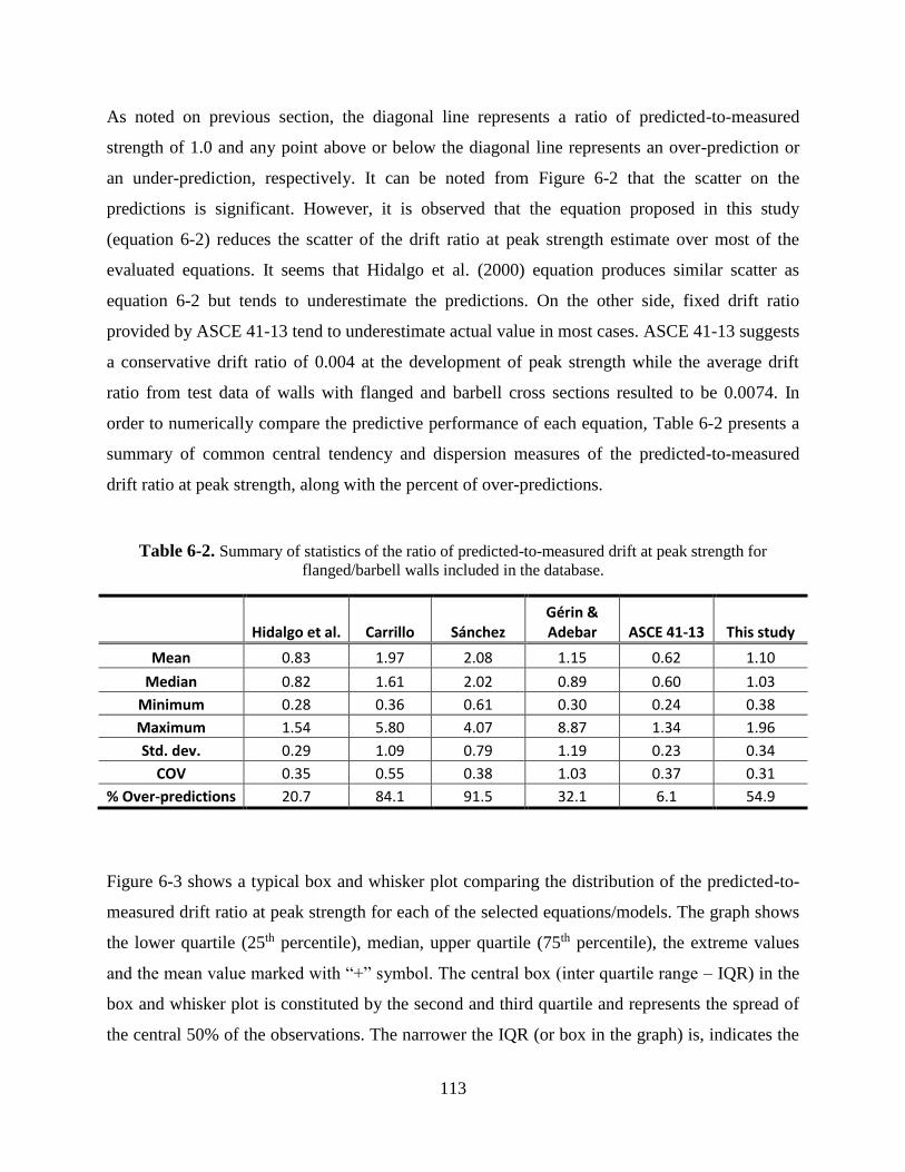
113

As noted on previous section, the diagonal line represents a ratio of predicted-to-measured



predictions is significant. However, it is observed that the equation proposed in this study

(equation 6-2) reduces the scatter of the drift ratio at peak strength estimate over most of the

evaluated equations. It seems that Hidalgo et al. (2000) equation produces similar scatter as

equation 6-2 but tends to underestimate the predictions. On the other side, fixed drift ratio

provided by ASCE 41-13 tend to underestimate actual value in most cases. ASCE 41-13 suggests

a conservative drift ratio of 0.004 at the development of peak strength while the average drift

ratio from test data of walls with flanged and barbell cross sections resulted to be 0.0074. In

order to numerically compare the predictive performance of each equation, Table 6-2 presents a

summary of common central tendency and dispersion measures of the predicted-to-measured

drift ratio at peak strength, along with the percent of over-predictions.

Table 6-2. Summary of statistics of the ratio of predicted-to-measured drift at peak strength for

flanged/barbell walls included in the database.


Mean 0.83 1.97 2.08 1.15 0.62 1.10

Median 0.82 1.61 2.02 0.89 0.60 1.03

Minimum 0.28 0.36 0.61 0.30 0.24 0.38

Maximum 1.54 5.80 4.07 8.87 1.34 1.96

Std. dev. 0.29 1.09 0.79 1.19 0.23 0.34

COV 0.35 0.55 0.38 1.03 0.37 0.31



measured drift ratio at peak strength for each of the selected equations/models. The graph shows

the lower quartile (25th percentile), median, upper quartile (75th percentile), the extreme values

and the mean value marked with “+” symbol. The central box (inter quartile range – IQR) in the

box and whisker plot is constituted by the second and third quartile and represents the spread of

the central 50% of the observations. The narrower the IQR (or box in the graph) is, indicates the

114

lesser the variability since the central 50% of the observations are nearer to the median value.

The lower and upper whiskers of the plot represent the spread of the first and fourth quartile,

being the ends of the whiskers the extreme (i.e. maximum and minimum) values marked with “-”

tick mark.

Figure 6-3. Distribution of the ratio of predicted-to-measured drift at peak strength.

From the statistics presented on Table 6-2 and from Figure 6-3, it can be observed that the

proposed equation produces an improved estimate of the drift ratio at peak strength since the

mean and median predicted-to-measured values are closer to 1.0, while the coefficient of

variation (COV) is kept in a similar level or lower than other predictions. It is also observed that

the midspread falls between 0.87 and 1.31, which means that the ratio of predicted-to-measured

values for 50% of the observations is closer to the median, and thus closer to a value of 1.0. In

the same manner, the proposed equation yields 54.9% of over-predictions which is very near to

the intended value of 50%.

In terms of the range (difference between maximum and minimum values), the equation

proposed in this study is on par with the estimates using ASCE 41-13 provisions and Hidalgo et

al. (2000) equations. However, these last two tend to underestimate the drift ratio at peak

strength as it can be noted from the low values of mean, median and % of over-predictions. On

the contrary, the predictions using the equations proposed by Carrillo (2010), Sánchez (2013),

0.00

1.00

2.00

3.00

4.00

5.00

6.00

0.00

1.00

2.00

3.00

4.00

5.00

6.00

Hidalgo etal.



Pre

dic

ted

dri

ft /

me

asu

red

dri

ft

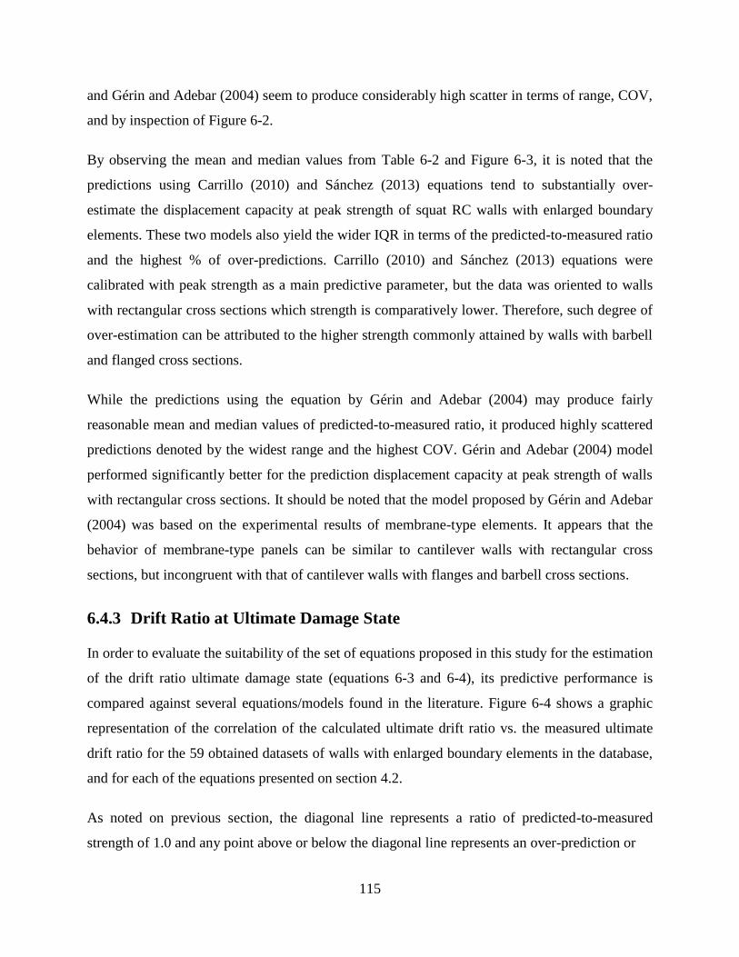
115

and Gérin and Adebar (2004) seem to produce considerably high scatter in terms of range, COV,

and by inspection of Figure 6-2.

By observing the mean and median values from Table 6-2 and Figure 6-3, it is noted that the

predictions using Carrillo (2010) and Sánchez (2013) equations tend to substantially over-

estimate the displacement capacity at peak strength of squat RC walls with enlarged boundary

elements. These two models also yield the wider IQR in terms of the predicted-to-measured ratio

and the highest % of over-predictions. Carrillo (2010) and Sánchez (2013) equations were

calibrated with peak strength as a main predictive parameter, but the data was oriented to walls

with rectangular cross sections which strength is comparatively lower. Therefore, such degree of

over-estimation can be attributed to the higher strength commonly attained by walls with barbell

and flanged cross sections.

While the predictions using the equation by Gérin and Adebar (2004) may produce fairly

reasonable mean and median values of predicted-to-measured ratio, it produced highly scattered

predictions denoted by the widest range and the highest COV. Gérin and Adebar (2004) model

performed significantly better for the prediction displacement capacity at peak strength of walls

with rectangular cross sections. It should be noted that the model proposed by Gérin and Adebar

(2004) was based on the experimental results of membrane-type elements. It appears that the

behavior of membrane-type panels can be similar to cantilever walls with rectangular cross

sections, but incongruent with that of cantilever walls with flanges and barbell cross sections.


In order to evaluate the suitability of the set of equations proposed in this study for the estimation

of the drift ratio ultimate damage state (equations 6-3 and 6-4), its predictive performance is

compared against several equations/models found in the literature. Figure 6-4 shows a graphic

representation of the correlation of the calculated ultimate drift ratio vs. the measured ultimate

drift ratio for the 59 obtained datasets of walls with enlarged boundary elements in the database,

and for each of the equations presented on section 4.2.

As noted on previous section, the diagonal line represents a ratio of predicted-to-measured


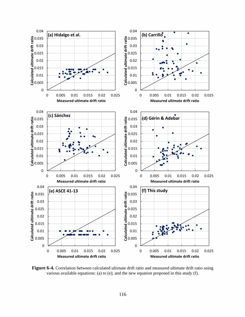
116

Figure 6-4. Correlation between calculated ultimate drift ratio and measured ultimate drift ratio using


0

0.005

0.01

0.015

0.02

0.025

0.03

0.035

0.04

0 0.005 0.01 0.015 0.02 0.025

Cal

cula

ted

ult

imat

e d

rift

rat

io


(a) Hidalgo et al.

0

0.005

0.01

0.015

0.02

0.025

0.03

0.035

0.04

0 0.005 0.01 0.015 0.02 0.025

Cal

cula

ted

ult

imat

e d

rift

rat

io


(b) Carrillo

0

0.005

0.01

0.015

0.02

0.025

0.03

0.035

0.04

0 0.005 0.01 0.015 0.02 0.025

Cal

cula

ted

ult

imat

e d

rift

rat

io


(c) Sánchez

0

0.005

0.01

0.015

0.02

0.025

0.03

0.035

0.04

0 0.005 0.01 0.015 0.02 0.025

Cal

cula

ted

ult

imat

e d

rift

rat

io


(d) Gérin & Adebar

0

0.005

0.01

0.015

0.02

0.025

0.03

0.035

0.04

0 0.005 0.01 0.015 0.02 0.025

Cal

cula

ted

ult

imat

e d

rift

rat

io


(e) ASCE 41-13

0

0.005

0.01

0.015

0.02

0.025

0.03

0.035

0.04

0 0.005 0.01 0.015 0.02 0.025

Cal

cula

ted

ult

imat

e d

rift

rat

io


(f) This study

117


predictions is significant. However, it is observed that the set of equations proposed in this study

(equations 6-3 and 6-4) reduces the scatter of the drift ratio at peak strength estimate over most

of the evaluated equations.

It seems that Hidalgo et al. (2000) equation produces similar scatter as equations 6-3 and 6-4, but

tends to over-estimate the predictions. On the other side, ASCE 41-13 provides fixed values of

the drift ratio at the ultimate state (abrupt strength drop) of 0.0075 and 0.010 for walls with low

axial loads and walls with significant axial loads, respectively. These provisions tend to

underestimate the actual value in most cases since the average drift ratio from test data resulted

to be 0.011. Also, by observing Figure 6-4(e) it is noted that most of the points fall below the

diagonal line.

Table 6-3. Summary of statistics of the ratio of predicted-to-measured ultimate drift for flanged/barbell

walls included in the database.


Mean 1.23 1.93 1.83 1.56 0.87 1.10

Median 1.19 1.76 1.70 1.09 0.85 1.06

Minimum 0.13 0.21 0.53 0.34 0.27 0.28

Maximum 2.44 4.82 3.52 13.59 2.26 2.30

Std. dev. 0.45 1.17 0.84 1.84 0.42 0.37

COV 0.37 0.61 0.46 1.19 0.48 0.34




drift ratio at peak strength, along with the percent of over-predictions. In the same fashion as

discussed on previous section (6.4.2), Figure 6-5 shows a typical box and whisker plot

comparing the distribution of the predicted-to-measured drift ratio for each selected

equations/models. The graph provides valuable information regarding the central tendency,

spread of values and extreme values.

118

Figure 6-5. Distribution of the ratio of predicted-to-measured ultimate drift.

From the statistics presented on Table 6-3 and from Figure 6-5, it can be observed that the

proposed set of equations produce an improved estimate of the drift ratio at peak strength since

the mean and median predicted-to-measured values are closer to 1.0, while the coefficient of

variation (COV) is kept in a similar level or lower than other predictions. It is also observed that

the midspread falls between 0.83 and 1.34, which means that the ratio of predicted-to-measured

values for 50% of the observations is closer to the median, and thus closer to a value of 1.0. In

the same manner, the proposed equation yields 55.9% of over-predictions which is very near to

the intended value of 50%.

In terms of the range (difference between maximum and minimum values), the equation

proposed in this study is on par with the estimates using ASCE 41-13 provisions and Hidalgo et

al. (2000) equations. However, ASCE 41-13 provisions tend to underestimate the drift ratio at

peak strength as it can be noted from the low values of mean, median, % of over-predictions, and

by inspection of Figure 6-4(e).

On the contrary, the predictions using the equations proposed by Carrillo (2010), Sánchez

(2013), and Gérin and Adebar (2004) seem to produce considerably high scatter in terms of

range, COV, and by inspection of Figure 6-4. Hidalgo et al. (2000) equations tend to slightly

over-estimate the ultimate drift capacity on an average sense.

0.00

0.50

1.00

1.50

2.00

2.50

3.00

3.50

4.00

4.50

5.00

0.00

0.50

1.00

1.50

2.00

2.50

3.00

3.50

4.00

4.50

5.00

Hidalgo etal.



Pre

dic

ted

dri

ft /

me

asu

red

dri

ft

119

By observing the mean and median values from Table 6-3 and Figure 6-5, it is noted that the

predictions using Carrillo (2010) and Sánchez (2013) equations tend to substantially over-

estimate the displacement capacity at peak strength of squat RC walls with enlarged boundary

elements. These two models also yield the widest IQR in terms of the predicted-to-measured

ratio and the highest % of over-predictions. The range of the predicted-to-measured ratio of these

two models is wider than all but the obtained using Gérin and Adebar (2004) equation. In the

same manner as for the displacement at peak strength, the higher strength commonly attained by

walls with barbell and flanged cross sections seems to bias the predictions of these two models

since both use the peak strength to predict the ultimate drift capacity.

While the predictions using the equation by Gérin and Adebar (2004) may produce fairly

reasonable median value of predicted-to-measured ratio, a considerable disparity is observed

between its mean and median values of 1.09 and 1.56, respectively, which represents a

significantly biased distribution. The equation by Gérin and Adebar (2004) produces highly

scattered predictions represented by the widest range and the highest COV. It is again observed

that Gérin and Adebar (2004) model performed significantly better for the prediction ultimate

drift capacity of walls with rectangular cross sections. It appears that the behavior of membrane-

type panels can be similar to cantilever walls with rectangular cross sections, but significantly

different to that of cantilever walls with flanges and barbell cross sections.

Finally, it was noted that the allowable drift ratios for RC shear wall building systems provided

on most current building design codes tend to be unconservative for squat RC walls with

enlarged boundary elements as well as for squat RC walls with rectangular cross sections. For

example, ASCE 7-10 seismic provisions allow a drift ratio of 0.02, while the average drift ratio

at ultimate damage state (20% strength degradation) obtained from the experimental values on

the collected database of squat walls with enlarged boundary elements was 0.011. This issue was

discussed in more detail on section 4.4.3.

120

ANALYTICAL MODELING OF SQUAT

WALLS

7.1 Introduction

As noted previously, squat RC shear walls tend to have shear-dominated behavior and to exhibit

strong coupling between flexural and shear responses. An adequate understanding of the lateral

load vs. deformation behavior along with analytical modeling tools that can simulate such

behavior is essential for the seismic design and performance assessment of nuclear power plant

structures and other low rise shear wall civil structures. This chapter evaluates the applicability

of two simplified modeling approaches for further calibration; and assesses their feasibility for

design and evaluation of squat RC walls.

Monotonic and cyclic analyses were performed within the OpenSees analytical platform. Data

from existing experimental tests of squat RC walls were used to develop and calibrate the

models. This chapter discusses the advantages and disadvantages of each method and provides

recommendations for future research in this topic. A Fiber-Based Model with flexure-shear

interaction and a Macro-Hysteretic Model available in the OpenSees analytical platform were

studied by comparing the simulated behavior with experimental data from several large scale

tests of RC squat walls with rectangular cross sections. Performed analyses show that both, the

Fiber-Based Model with shear-flexure interaction and the Macro-Hysteretic models can be

calibrated to obtain a reasonable prediction of the lateral load-displacement behavior of squat

reinforced concrete walls. Finally, the backbones for the presented Macro-Hysteretic model were

calculated using the expressions for the prediction of strength and displacement capacity

developed in previous chapters (Chapters 3 to 6) and analyses were performed to simulate the

cyclic behavior of several large scale RC squat walls with rectangular cross sections. The

obtained analysis results were then compared to experimental data for the corresponding test

specimens.

The experimental data considered on this chapter was obtained from experimental tests of twelve

large-size, low aspect ratio, RC shear walls that were conducted at the University at Buffalo

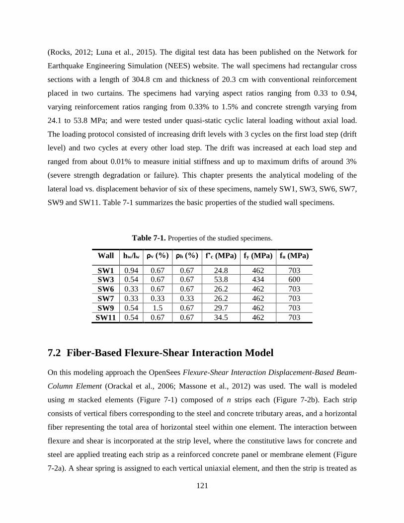
121

(Rocks, 2012; Luna et al., 2015). The digital test data has been published on the Network for

Earthquake Engineering Simulation (NEES) website. The wall specimens had rectangular cross

sections with a length of 304.8 cm and thickness of 20.3 cm with conventional reinforcement

placed in two curtains. The specimens had varying aspect ratios ranging from 0.33 to 0.94,

varying reinforcement ratios ranging from 0.33% to 1.5% and concrete strength varying from

24.1 to 53.8 MPa; and were tested under quasi-static cyclic lateral loading without axial load.

The loading protocol consisted of increasing drift levels with 3 cycles on the first load step (drift

level) and two cycles at every other load step. The drift was increased at each load step and

ranged from about 0.01% to measure initial stiffness and up to maximum drifts of around 3%

(severe strength degradation or failure). This chapter presents the analytical modeling of the

lateral load vs. displacement behavior of six of these specimens, namely SW1, SW3, SW6, SW7,

SW9 and SW11. Table 7-1 summarizes the basic properties of the studied wall specimens.

Table 7-1. Properties of the studied specimens.

Wall hw/lw ρv (%) ρh (%) f’c (MPa) fy (MPa) fu (MPa)

SW1 0.94 0.67 0.67 24.8 462 703

SW3 0.54 0.67 0.67 53.8 434 600

SW6 0.33 0.67 0.67 26.2 462 703

SW7 0.33 0.33 0.33 26.2 462 703

SW9 0.54 1.5 0.67 29.7 462 703

SW11 0.54 0.67 0.67 34.5 462 703

7.2 Fiber-Based Flexure-Shear Interaction Model

On this modeling approach the OpenSees Flexure-Shear Interaction Displacement-Based Beam-

Column Element (Orackal et al., 2006; Massone et al., 2012) was used. The wall is modeled

using m stacked elements (Figure 7-1) composed of n strips each (Figure 7-2b). Each strip

consists of vertical fibers corresponding to the steel and concrete tributary areas, and a horizontal

fiber representing the total area of horizontal steel within one element. The interaction between

flexure and shear is incorporated at the strip level, where the constitutive laws for concrete and

steel are applied treating each strip as a reinforced concrete panel or membrane element (Figure

7-2a). A shear spring is assigned to each vertical uniaxial element, and then the strip is treated as

122

an RC panel with membrane action (i.e., with uniform normal and shear stresses applied in the

plane) as shown in Figure 7-2(a). A rotating-angle softened-truss-model (Pang and Hsu, 1995)

approach is implemented to represent the membrane (panel) behavior. Constitutive stress-strain

material models are applied along the principal strain field, to obtain the stresses in the principal

directions and then transformed to the reference (x, y) coordinates in order to obtain forces in the

global directions. In this formulation, it is assumed that the principal stress and strain directions

coincide. The parameter c (Figure 7-2(a)) is called the element center of rotation factor and is

defined as the relative distance from the bottom of the element to the center of rotation. Massone

(2006) suggested a value of c = 0.4 which was adopted in this study.

Figure 7-1. Wall model using Flexure-Shear Interaction Displacement-Based Beam-Column Element

(Adapted from Massone, 2010a).

(a) (b)

Figure 7-2. Flexure-Shear Interaction Displacement-Based Beam-Column Element: (a) model element

(adapted from Orackal et al., 2006), and (b) element section modeling (Massone et al., 2012).

m

.

.

.

.

.

.

3

2

1

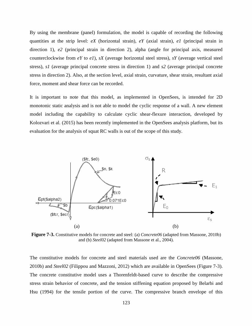
123

By using the membrane (panel) formulation, the model is capable of recording the following

quantities at the strip level: eX (horizontal strain), eY (axial strain), e1 (principal strain in

direction 1), e2 (principal strain in direction 2), alpha (angle for principal axis, measured

counterclockwise from eY to e1), sX (average horizontal steel stress), sY (average vertical steel

stress), s1 (average principal concrete stress in direction 1) and s2 (average principal concrete

stress in direction 2). Also, at the section level, axial strain, curvature, shear strain, resultant axial

force, moment and shear force can be recorded.

It is important to note that this model, as implemented in OpenSees, is intended for 2D

monotonic static analysis and is not able to model the cyclic response of a wall. A new element

model including the capability to calculate cyclic shear-flexure interaction, developed by

Kolozvari et al. (2015) has been recently implemented in the OpenSees analysis platform, but its

evaluation for the analysis of squat RC walls is out of the scope of this study.

(a) (b)

Figure 7-3. Constitutive models for concrete and steel: (a) Concrete06 (adapted from Massone, 2010b)

and (b) Steel02 (adapted from Massone et al., 2004).

The constitutive models for concrete and steel materials used are the Concrete06 (Massone,

2010b) and Steel02 (Filippou and Mazzoni, 2012) which are available in OpenSees (Figure 7-3).

The concrete constitutive model uses a Thorenfeldt-based curve to describe the compressive

stress strain behavior of concrete, and the tension stiffening equation proposed by Belarbi and

Hsu (1994) for the tensile portion of the curve. The compressive branch envelope of this

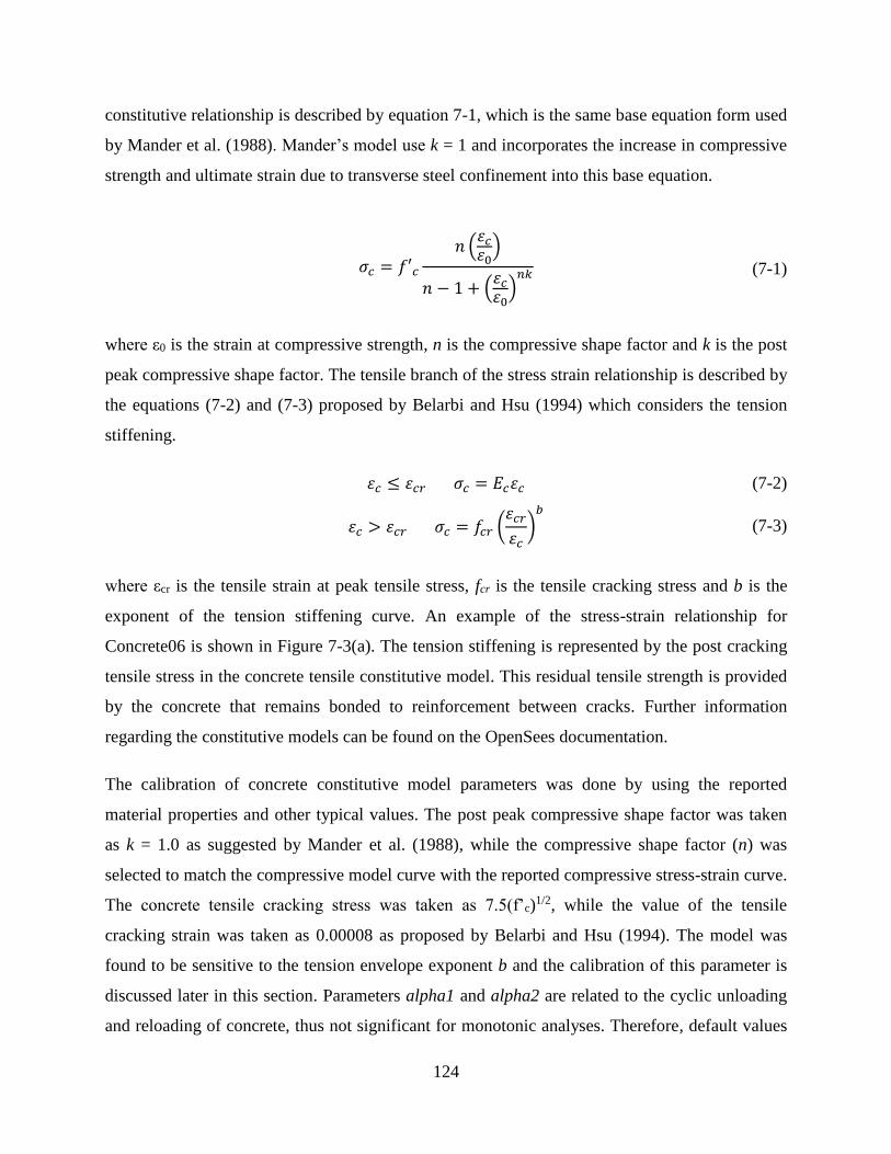
http://opensees.berkeley.edu/wiki/images/c/c6/Concrete06C.png

124

constitutive relationship is described by equation 7-1, which is the same base equation form used

by Mander et al. (1988). Mander’s model use k = 1 and incorporates the increase in compressive

strength and ultimate strain due to transverse steel confinement into this base equation.

𝜎𝑐 = 𝑓′𝑐

𝑛 (𝜀𝑐

𝜀0)

𝑛 − 1 + (𝜀𝑐

𝜀0)

𝑛𝑘 (7-1)

where ε0 is the strain at compressive strength, n is the compressive shape factor and k is the post

peak compressive shape factor. The tensile branch of the stress strain relationship is described by

the equations (7-2) and (7-3) proposed by Belarbi and Hsu (1994) which considers the tension

stiffening.

𝜀𝑐 ≤ 𝜀𝑐𝑟 𝜎𝑐 = 𝐸𝑐𝜀𝑐 (7-2)

𝜀𝑐 > 𝜀𝑐𝑟 𝜎𝑐 = 𝑓𝑐𝑟 (𝜀𝑐𝑟

𝜀𝑐)

𝑏

(7-3)

where εcr is the tensile strain at peak tensile stress, fcr is the tensile cracking stress and b is the

exponent of the tension stiffening curve. An example of the stress-strain relationship for

Concrete06 is shown in Figure 7-3(a). The tension stiffening is represented by the post cracking

tensile stress in the concrete tensile constitutive model. This residual tensile strength is provided

by the concrete that remains bonded to reinforcement between cracks. Further information

regarding the constitutive models can be found on the OpenSees documentation.

The calibration of concrete constitutive model parameters was done by using the reported

material properties and other typical values. The post peak compressive shape factor was taken

as k = 1.0 as suggested by Mander et al. (1988), while the compressive shape factor (n) was

selected to match the compressive model curve with the reported compressive stress-strain curve.

The concrete tensile cracking stress was taken as 7.5(f’c)1/2, while the value of the tensile

cracking strain was taken as 0.00008 as proposed by Belarbi and Hsu (1994). The model was

found to be sensitive to the tension envelope exponent b and the calibration of this parameter is

discussed later in this section. Parameters alpha1 and alpha2 are related to the cyclic unloading

and reloading of concrete, thus not significant for monotonic analyses. Therefore, default values

125

were used. Table 7-2 shows the parameters used in the analyses for the concrete constitutive

model. Negative values on Table 7-2 indicate compressive concrete related parameters.

Table 7-2. Concrete06 constitutive model calibrated parameters.

Wall fc

(MPa) e0 n k alpha1 fcr ecr b alpha2

SW1 - 24.8 -0.003 2.0 1.0 0.32 450.0 0.00008 4.0 0.08

SW3 - 53.8 -0.003 3.75 1.0 0.32 662.4 0.00008 4.0 0.08

SW6 - 26.2 -0.003 2.0 1.0 0.32 462.3 0.00008 4.0 0.08

The reinforcement is modeled using the monotonic branch of uniaxial material model Steel02

available in OpenSees. This constitutive model is based on the model described by Filippou et al.

(1983) and uses a simple bi-linear relationship with a softened transition between the initial and

post-yield tangents as shown in Figure 7-3(b). Further information regarding the constitutive

models can be found on the OpenSees documentation.

Calibration of constitutive model parameters for the reinforcing steel was obtained from the

reported material properties. Nevertheless, some parameters require experimental data from

cyclic tests which is not usually available. Therefore, the values of R0, cR1 and cR2 were taken

from recommended values found on the OpenSees documentation and the values for the

hardening parameters a1 and a2 calibrated with experimental data by prior researchers were

obtained from Elmorsi et al. (1998). Default values were used for a3 and a4 (no hardening in

tension was considered). However, these isotropic hardening parameters are not as significant for

monotonic analyses as they are for cyclic analyses. Table 7-3 presents the parameters used for

the steel constitutive model.

Table 7-3. Steel02 constitutive model calibrated parameters.

Wall fy

(MPa)

E0

(MPa) bs R0 cR1 cR2 a1 a2 a3 a4

SW1 462 200x103 0.018 15 0.925 0.15 18.5 0.0015 0 1.0

SW3 434 200x103 0.013 15 0.925 0.15 18.5 0.0015 0 1.0

SW6 462 200x103 0.018 15 0.925 0.15 18.5 0.0015 0 1.0

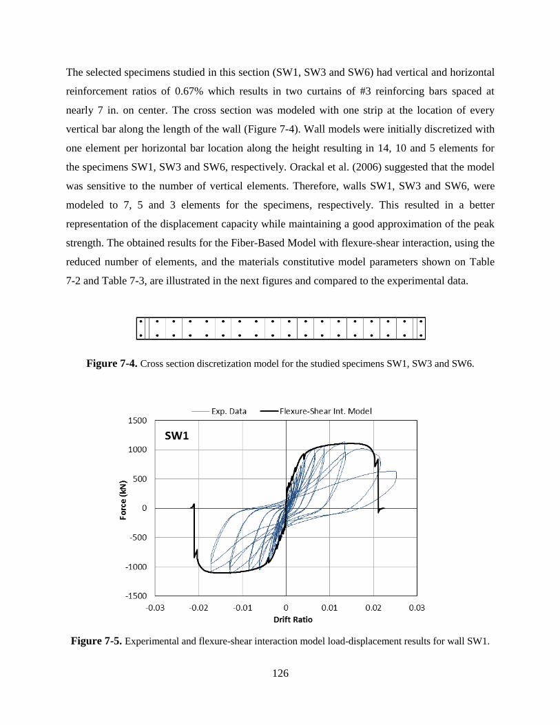
126

The selected specimens studied in this section (SW1, SW3 and SW6) had vertical and horizontal

reinforcement ratios of 0.67% which results in two curtains of #3 reinforcing bars spaced at

nearly 7 in. on center. The cross section was modeled with one strip at the location of every

vertical bar along the length of the wall (Figure 7-4). Wall models were initially discretized with

one element per horizontal bar location along the height resulting in 14, 10 and 5 elements for

the specimens SW1, SW3 and SW6, respectively. Orackal et al. (2006) suggested that the model

was sensitive to the number of vertical elements. Therefore, walls SW1, SW3 and SW6, were

modeled to 7, 5 and 3 elements for the specimens, respectively. This resulted in a better

representation of the displacement capacity while maintaining a good approximation of the peak

strength. The obtained results for the Fiber-Based Model with flexure-shear interaction, using the

reduced number of elements, and the materials constitutive model parameters shown on Table

7-2 and Table 7-3, are illustrated in the next figures and compared to the experimental data.

Figure 7-4. Cross section discretization model for the studied specimens SW1, SW3 and SW6.

Figure 7-5. Experimental and flexure-shear interaction model load-displacement results for wall SW1.

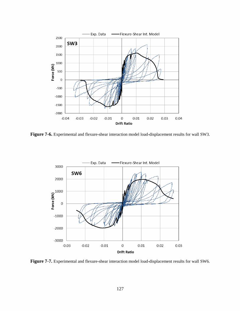
127



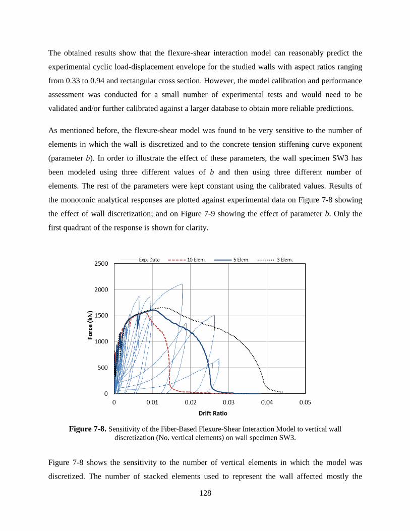
128

The obtained results show that the flexure-shear interaction model can reasonably predict the

experimental cyclic load-displacement envelope for the studied walls with aspect ratios ranging

from 0.33 to 0.94 and rectangular cross section. However, the model calibration and performance

assessment was conducted for a small number of experimental tests and would need to be

validated and/or further calibrated against a larger database to obtain more reliable predictions.

As mentioned before, the flexure-shear model was found to be very sensitive to the number of

elements in which the wall is discretized and to the concrete tension stiffening curve exponent

(parameter b). In order to illustrate the effect of these parameters, the wall specimen SW3 has

been modeled using three different values of b and then using three different number of

elements. The rest of the parameters were kept constant using the calibrated values. Results of

the monotonic analytical responses are plotted against experimental data on Figure 7-8 showing

the effect of wall discretization; and on Figure 7-9 showing the effect of parameter b. Only the

first quadrant of the response is shown for clarity.

Figure 7-8. Sensitivity of the Fiber-Based Flexure-Shear Interaction Model to vertical wall

discretization (No. vertical elements) on wall specimen SW3.

Figure 7-8 shows the sensitivity to the number of vertical elements in which the model was

discretized. The number of stacked elements used to represent the wall affected mostly the

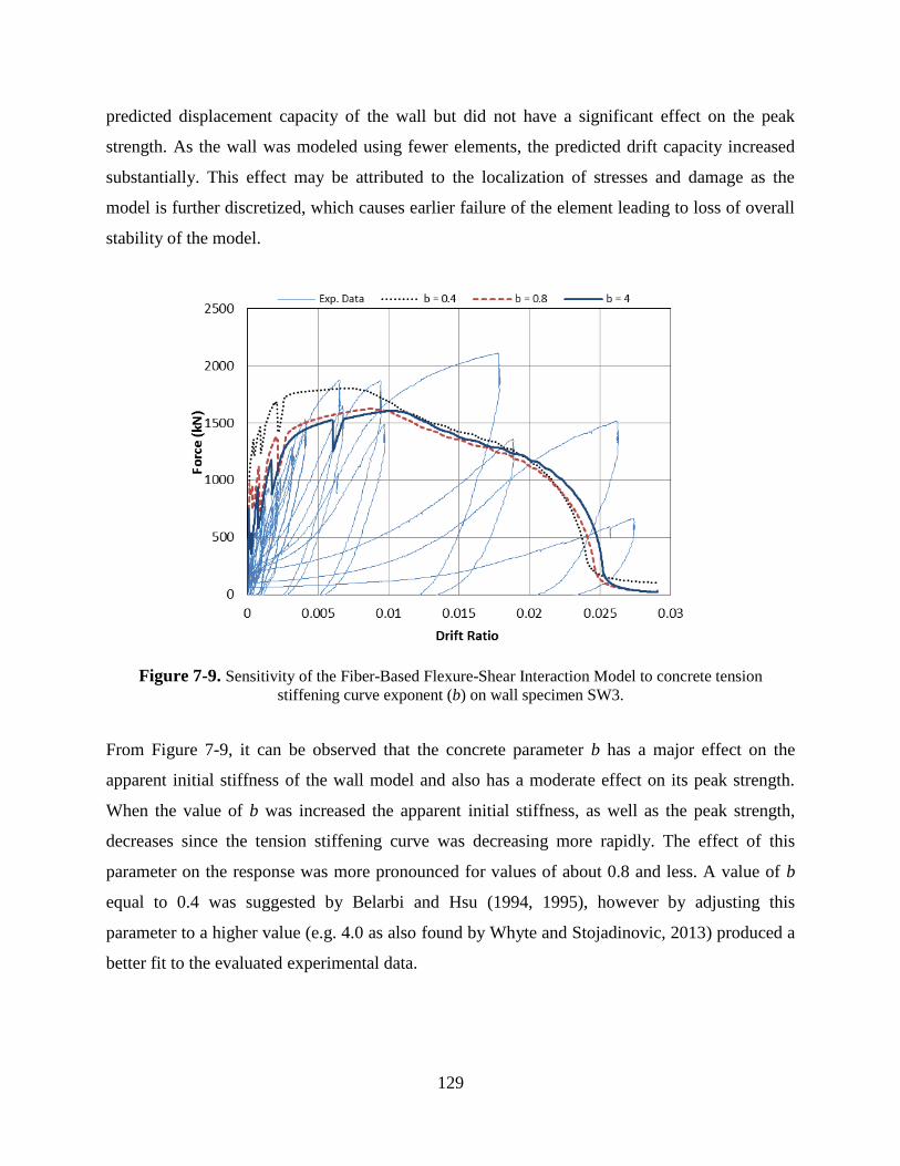
129

predicted displacement capacity of the wall but did not have a significant effect on the peak

strength. As the wall was modeled using fewer elements, the predicted drift capacity increased

substantially. This effect may be attributed to the localization of stresses and damage as the

model is further discretized, which causes earlier failure of the element leading to loss of overall

stability of the model.

Figure 7-9. Sensitivity of the Fiber-Based Flexure-Shear Interaction Model to concrete tension

stiffening curve exponent (b) on wall specimen SW3.

From Figure 7-9, it can be observed that the concrete parameter b has a major effect on the

apparent initial stiffness of the wall model and also has a moderate effect on its peak strength.

When the value of b was increased the apparent initial stiffness, as well as the peak strength,

decreases since the tension stiffening curve was decreasing more rapidly. The effect of this

parameter on the response was more pronounced for values of about 0.8 and less. A value of b

equal to 0.4 was suggested by Belarbi and Hsu (1994, 1995), however by adjusting this

parameter to a higher value (e.g. 4.0 as also found by Whyte and Stojadinovic, 2013) produced a

better fit to the evaluated experimental data.

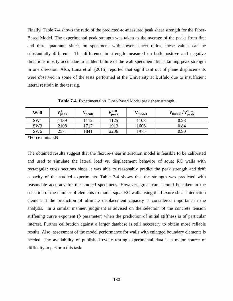
130

Finally, Table 7-4 shows the ratio of the predicted-to-measured peak shear strength for the Fiber-

Based Model. The experimental peak strength was taken as the average of the peaks from first

and third quadrants since, on specimens with lower aspect ratios, these values can be

substantially different. The difference in strength measured on both positive and negative

directions mostly occur due to sudden failure of the wall specimen after attaining peak strength

in one direction. Also, Luna et al. (2015) reported that significant out of plane displacements

were observed in some of the tests performed at the University at Buffalo due to insufficient

lateral restrain in the test rig.

Table 7-4. Experimental vs. Fiber-Based Model peak shear strength.

Wall 𝐕𝐩𝐞𝐚𝐤+ 𝐕𝐩𝐞𝐚𝐤

− 𝐕𝐩𝐞𝐚𝐤𝐚𝐯𝐠

𝐕𝐦𝐨𝐝𝐞𝐥 𝐕𝐦𝐨𝐝𝐞𝐥 𝐕𝐩𝐞𝐚𝐤𝒂𝒗𝒈

⁄

SW1 1139 1112 1125 1108 0.98

SW3 2108 1717 1913 1606 0.84

SW6 2571 1841 2206 1975 0.90

*Force units: kN

The obtained results suggest that the flexure-shear interaction model is feasible to be calibrated

and used to simulate the lateral load vs. displacement behavior of squat RC walls with

rectangular cross sections since it was able to reasonably predict the peak strength and drift

capacity of the studied experiments. Table 7-4 shows that the strength was predicted with

reasonable accuracy for the studied specimens. However, great care should be taken in the

selection of the number of elements to model squat RC walls using the flexure-shear interaction

element if the prediction of ultimate displacement capacity is considered important in the

analysis. In a similar manner, judgment is advised on the selection of the concrete tension

stiffening curve exponent (b parameter) when the prediction of initial stiffness is of particular

interest. Further calibration against a larger database is still necessary to obtain more reliable

results. Also, assessment of the model performance for walls with enlarged boundary elements is

needed. The availability of published cyclic testing experimental data is a major source of

difficulty to perform this task.

131

7.3 Macro-Hysteretic Model

In this modeling approach the cyclic lateral load vs. displacement behavior of the wall was

modeled as a single degree of freedom structure and the experimental displacements were

applied at the free end. The hysteretic material model from OpenSees called Hysteretic Material

(Scott and Filippou, 2013) was used. This model requires the definition of a backbone curve as

shown in Figure 7-10, which was calibrated with the experimental data.

Figure 7-10. Backbone curve definition parameters for the hysteretic material model (Scott and

Filippou, 2013).

The Hysteretic Material model has the capability to capture commonly observed pinching and

strength and stiffness degradation of hysteresis loops. This can be accomplished by the

calibration of the model with experimental data. In order to illustrate the effect of each of the

model parameters Figure 7-11 is presented. Figure 7-11(a) shows an example of the effect of the

pinching parameters (pinchX and pinchY) where the black line corresponds to both parameters

set to a value of 1.0 (no pinching), while the red line corresponds to pinchX = 0.8 and pinchY =

0.2. Note that the pinchX parameter is the pinching factor for deformation during reloading,

while the pinchY parameter corresponds to the pinching factor for force during reloading.

The model has two strength-reducing damage parameters referred to as damage1 and damage2.

The damage1 parameter incorporates strength deterioration due to ductility, whereas the

damage2 parameter incorporates strength deterioration damage due to the energy dissipated by

132

inelastic deformation. This means that the first produces a strength reduction proportional to the

cumulative plastic deformation, while the second produces a strength reduction proportional to

the cumulative inelastic energy dissipation. Figure 7-11(b) shows an example of the effect of

strength degradation parameters where the black line corresponds to both damage parameters set

to zero (no damage) and the red line corresponds to damage parameters higher than zero.

This model also includes a parameter to adjust unloading stiffness degradation based on the

ductility demand (beta). This parameter is the power used to determine ductility-dependent

degraded unloading stiffness as a portion of the initial unloading stiffness (μ-beta). Figure 7-11(c)

shows an example of the effect of unloading stiffness degradation parameter where the black line

corresponds to beta = 0 (no damage), and the red line corresponds to beta = 0.5.

(a) (b) (c)

Figure 7-11. Effect of hysteretic parameters on the Hysteretic Material model: (a) pinching, (b) strength

degradation, (c) and unloading stiffness degradation (Scott and Filippou, 2013).

7.3.1 Basic Parameters Calibration

The calculated backbone curve was optimized by taking the peak strength and maximum drift

points equal to the experimental values. The initial stiffness was also set to be equal to the

obtained experimentally. The control point associated with the “yielding”, or cracking in the case

133

of shear-controlled squat RC walls, was adjusted so that the area under the experimental cyclic

envelope equals the area under the calculated backbone (Figure 7-12).

Table 7-5 shows the calculated backbone parameters for the considered walls. The intent of

calibrating the backbone curve to the experimental envelope was to evaluate if the tri-linear

backbone is capable of reasonably represent the experimental load-displacement envelopes, and

afterwards, to assess the model’s ability to capture the hysteretic behavior of the considered

walls by calibrating the hysteretic parameters. From this calibration, initial values for the

Hysteretic Model parameters were identified for modeling squat RC walls. The intent was not to

provide a statistically robust calibration of the hysteresis parameters, but to identify a reasonable

range of values for the parameters and show the capability of the simple model to capture the

typical hysteretic behavior of these walls.

(a) Experimental cyclic envelope (b) Backbone curve fitting

Figure 7-12. Example backbone curve fitting for the Macro-Hysteretic Model (SW1).

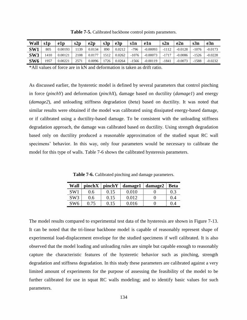
134

Table 7-5. Calibrated backbone control points parameters.

Wall s1p e1p s2p e2p s3p e3p s1n e1n s2n e2n s3n e3n

SW1 805 0.00193 1139 0.0134 890 0.0212 -796 -0.00093 -1112 -0.0128 -1076 -0.0173

SW3 1410 0.00121 2108 0.0177 1512 0.0262 -1076 -0.00073 -1717 -0.0086 -1526 -0.0228

SW6 1957 0.00221 2571 0.0096 1726 0.0264 -1566 -0.00119 -1841 -0.0073 -1588 -0.0232

*All values of force are in kN and deformation is taken as drift ratio.

As discussed earlier, the hysteretic model is defined by several parameters that control pinching

in force (pinchY) and deformation (pinchX), damage based on ductility (damage1) and energy

(damage2), and unloading stiffness degradation (beta) based on ductility. It was noted that

similar results were obtained if the model was calibrated using dissipated energy-based damage,

or if calibrated using a ductility-based damage. To be consistent with the unloading stiffness

degradation approach, the damage was calibrated based on ductility. Using strength degradation

based only on ductility produced a reasonable approximation of the studied squat RC wall

specimens’ behavior. In this way, only four parameters would be necessary to calibrate the

model for this type of walls. Table 7-6 shows the calibrated hysteresis parameters.

Table 7-6. Calibrated pinching and damage parameters.

Wall pinchX pinchY damage1 damage2 Beta

SW1 0.6 0.15 0.010 0 0.3

SW3 0.6 0.15 0.012 0 0.4

SW6 0.75 0.15 0.016 0 0.4

The model results compared to experimental test data of the hysteresis are shown in Figure 7-13.

It can be noted that the tri-linear backbone model is capable of reasonably represent shape of

experimental load-displacement envelope for the studied specimens if well calibrated. It is also

observed that the model loading and unloading rules are simple but capable enough to reasonably

capture the characteristic features of the hysteretic behavior such as pinching, strength

degradation and stiffness degradation. In this study these parameters are calibrated against a very

limited amount of experiments for the purpose of assessing the feasibility of the model to be

further calibrated for use in squat RC walls modeling; and to identify basic values for such

parameters.

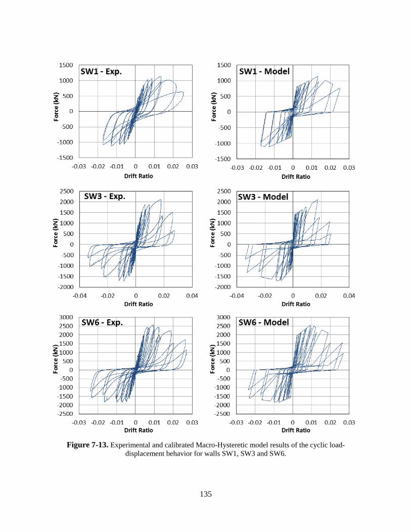
135

Figure 7-13. Experimental and calibrated Macro-Hysteretic model results of the cyclic load-

displacement behavior for walls SW1, SW3 and SW6.

136

One of the limitations of the Hysteretic Material model is that the backbone curve has only three

linear segments. These types of walls and other shear-controlled RC structural members tend to

show an initial stiffness reduction upon flexural cracking. Then they would experience a larger

reduction in stiffness at the “yielding” point (which is not necessarily related to the yielding of

the reinforcement but more likely to significant diagonal cracking) until it reaches the peak

strength or “capping point”, where the strength degradation becomes more pronounced and the

slope of the envelope becomes negative until reaching failure. While this behavior would be

more accurately modeled with the incorporation of a fourth line segment into the backbone curve

to include the flexural cracking point, the stiffness reduction due to diagonal cracking appears to

be more significant, and therefore, the tri-linear backbone can reasonably capture the typical

experimental load-displacement envelope shape of members controlled by shear.

Among the most significant advantages of Macro-Hysteretic model over the Fiber-Based

Flexure-Shear Interaction Model presented herein are the substantially less computational effort

and the ability to simulate the cyclic performance of a wall with reasonable accuracy. Also, the

use of simplified Macro-Hysteretic models for structures that include squat walls would be

generally preferred for performance based assessment of structures due to their ability to

represent the cyclic force-deformation behavior at the story level with relative simplicity. This

model can be conveniently calibrated to fit a given experimental dataset since it has fewer

pinching and degradation parameters than other hysteretic models that have been proposed in

literature. Despite the few parameters required, it is shown that the Hysteretic Material can

reasonably capture the key characteristics of the hysteretic behavior of squat walls with

rectangular cross sections. Having a calibrated model to determine the backbone control points,

such as the equations proposed in Chapters 3 to 6, is key to use this model for the simulation of

squat RC walls behavior. The simplicity of the model makes it suitable for empirical calibration

of the backbone and hysteresis parameters with a larger database which would allow to use this

model to simulate the behavior of squat RC walls with reasonable accuracy and without the need

of having experimental data available.

137

7.3.2 Developed Backbone Model

On previous section (7.3.1) it was shown that the experimental load displacement envelope of a

squat RC wall can be reasonably represented with a tri-linear backbone. On Chapters 4 and 6 it

was noted that these walls show a first major stiffness reduction that is associated with the

occurrence of significant diagonal cracking. This point was associated to a characteristic lateral

force level of 0.6 Vpeak. Then the wall would keep developing lateral strength until reaching the

peak strength, where the strength degradation becomes more noticeable, and the strength

envelope will start to decrease in a pronounced manner as the displacement is increased. This

behavior can be represented with a straight line of negative slope. While several walls were taken

to extreme strength degradation levels showing considerable energy dissipation, data for these

advanced damage states was very scarce, and therefore predictions of behavior derived thereof

would be considered unreliable. To these effects, ultimate damage state was defined using a

conventional 20% strength drop criterion (when attaining 0.8Vpeak).

Calibrated expressions obtained from multiple linear regression analyses were proposed on

Chapters 4 and 6 for the determination of the drift ratio capacity at each of the control points (i.e.

diagonal cracking, peak strength, and ultimate damage state), for walls with rectangular cross

sections and with enlarged boundary elements, respectively. Likewise, expressions were

proposed on Chapters 3 and 5, for the prediction of the peak strength of squat RC walls with

rectangular cross section and with enlarged boundary elements, respectively. Using the

aforementioned sets of expressions, the proposed tri-linear backbone curve can be estimated by

determining the three control points: cracking point (Rcr , 0.6Vpeak), peak point (Rpeak , Vpeak), and

ultimate state point (Ru , 0.8Vpeak).

Figure 7-14 and Figure 7-15 show the calculated backbones using the methodology proposed

herein, compared to the experimental load-drift ratio envelope for several squat RC walls of

rectangular cross sections and with enlarged boundary elements, respectively. The studied wall

specimens were selected from different research programs within the assembled database and

have variety of characteristics (e.g. aspect ratio, reinforcement ratios concrete strength, etc.). The

specimens with rectangular cross section shown on Figure 7-14 were selected from the test

programs by Carrillo and Alcocer (2013), Terzioğlu (2011), Luna et al. (2015),

Saatcioglu/Wiradinata (1985), and Park et al. (2015). The specimens with enlarged boundary

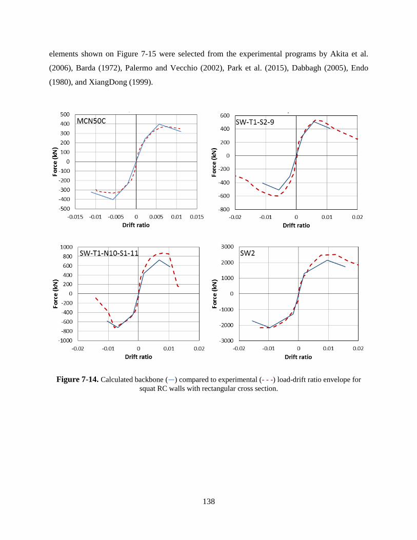
138

elements shown on Figure 7-15 were selected from the experimental programs by Akita et al.

(2006), Barda (1972), Palermo and Vecchio (2002), Park et al. (2015), Dabbagh (2005), Endo

(1980), and XiangDong (1999).

Figure 7-14. Calculated backbone (―) compared to experimental (- - -) load-drift ratio envelope for

squat RC walls with rectangular cross section.

139

Figure 7.14. Continued.

140

Figure 7-15. Calculated backbone (―) compared to experimental (- - -) load-drift ratio envelope for

squat RC walls with enlarged boundary elements.

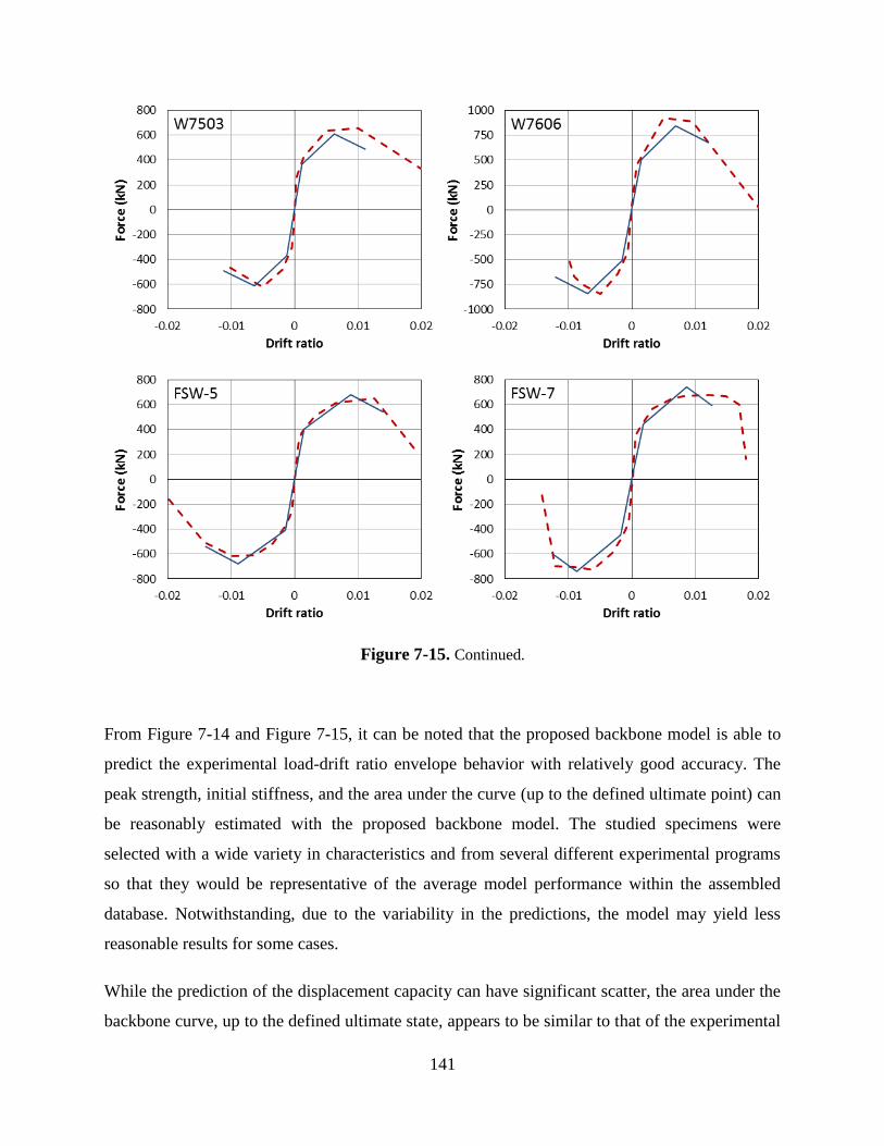
141

Figure 7-15. Continued.

From Figure 7-14 and Figure 7-15, it can be noted that the proposed backbone model is able to

predict the experimental load-drift ratio envelope behavior with relatively good accuracy. The

peak strength, initial stiffness, and the area under the curve (up to the defined ultimate point) can

be reasonably estimated with the proposed backbone model. The studied specimens were

selected with a wide variety in characteristics and from several different experimental programs

so that they would be representative of the average model performance within the assembled

database. Notwithstanding, due to the variability in the predictions, the model may yield less

reasonable results for some cases.

While the prediction of the displacement capacity can have significant scatter, the area under the

backbone curve, up to the defined ultimate state, appears to be similar to that of the experimental

142

envelope. This indicates that the proposed backbone model can adequately simulate the energy

dissipation characteristics of squat RC walls under monotonic lateral loading. In the same

manner, these findings suggest that the proposed backbone model, when used in conjunction

with a hysteretic model, can reasonably represent the cyclic energy dissipation of squat RC

walls; provided that the hysteresis damage parameters of the model (i.e. pinching, strength

degradation and stiffness degradation) are well calibrated.

The next section discusses the analysis results for several walls using the Macro-Hysteretic

model (OpenSees Hysteretic Material model) presented earlier in this chapter, with the basic

calibration of hysteretic parameters presented on section 7.3.1 in conjunction with the backbone

model proposed herein.

7.3.3 Macro-Hysteretic Model using Developed Backbone Model

As it was shown on previous section, the proposed tri-linear backbone model, using the

equations developed in Chapters 3 to 6 to determine its control points, is capable of reasonably

estimate the experimental load-drift ratio behavior of the studied walls. Furthermore, if the

backbone and hysteretic parameters are well calibrated against experimental data, the presented

Macro-Hysteretic model is capable of simulating the experimental hysteretic behavior with very

good accuracy. In this section an additional three walls from the Luna et al. (2015)/NEES-UB

experimental program were modeled using the proposed Macro-Hysteretic model (OpenSees

Hysteretic Material model) presented earlier in this chapter, with the hysteretic parameters

identified by the basic calibration presented on section 7.3.1, and with the calibrated backbone

model discussed on previous section (7.3.2). The calculated backbone control points are shown

on Table 7-7 and the selected hysteretic parameters are shown on Table 7-8.

Table 7-7. Calculated backbone control points parameters.

Wall s1p e1p s2p e2p s3p e3p s1n e1n s2n e2n s3n e3n

SW7 803 0.0013 1338 0.0076 1071 0.0132 -803 -0.0013 -1338 -0.0076 -1071 -0.0132

SW9 1581 0.0016 2635 0.0082 2108 0.0152 -1581 -0.0016 -2635 -0.0082 -2108 -0.0152

SW11 1147 0.0019 1912 0.0085 1529 0.0147 -1147 -0.0019 -1912 -0.0085 -1529 -0.0147

*All values of force are in kN and deformation is taken as drift ratio.

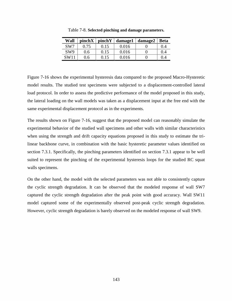
143

Table 7-8. Selected pinching and damage parameters.

Wall pinchX pinchY damage1 damage2 Beta

SW7 0.75 0.15 0.016 0 0.4

SW9 0.6 0.15 0.016 0 0.4

SW11 0.6 0.15 0.016 0 0.4

Figure 7-16 shows the experimental hysteresis data compared to the proposed Macro-Hysteretic

model results. The studied test specimens were subjected to a displacement-controlled lateral

load protocol. In order to assess the predictive performance of the model proposed in this study,

the lateral loading on the wall models was taken as a displacement input at the free end with the

same experimental displacement protocol as in the experiments.

The results shown on Figure 7-16, suggest that the proposed model can reasonably simulate the

experimental behavior of the studied wall specimens and other walls with similar characteristics

when using the strength and drift capacity equations proposed in this study to estimate the tri-

linear backbone curve, in combination with the basic hysteretic parameter values identified on

section 7.3.1. Specifically, the pinching parameters identified on section 7.3.1 appear to be well

suited to represent the pinching of the experimental hysteresis loops for the studied RC squat

walls specimens.

On the other hand, the model with the selected parameters was not able to consistently capture

the cyclic strength degradation. It can be observed that the modeled response of wall SW7

captured the cyclic strength degradation after the peak point with good accuracy. Wall SW11

model captured some of the experimentally observed post-peak cyclic strength degradation.

However, cyclic strength degradation is barely observed on the modeled response of wall SW9.

144

Figure 7-16. Experimental and Macro-Hysteretic model results of the cyclic load- displacement

behavior for walls SW7, SW9 and SW11 using calculated backbone and base hysteretic parameters.

145

The Macro-Hysteretic model starts to show significant strength degradation after the peak point

is reached. Prior to the peak point the model does not show noticeable strength degradation. The

strength degradation on the model increases with further cycling past the peak point, which is

also observed on the experimental response. However, due to the differences between the

displacement at peak strength of the estimated backbone and the actual (experimental)

displacement at peak strength, the model may start to degrade in strength at a different stage than

in the test. It is observed that the estimated displacement at peak strength is larger than the

corresponding experimental value for all the three walls studied in this section. Notwithstanding,

walls SW7, SW11 and SW9 undertook six, four, and three full cycles past the peak control point,

respectively. That explains the observed differences in cyclic strength degradation where wall

SW7 showed the highest degradation while wall SW9 showed the lowest degradation.

In terms of the unloading stiffness degradation, the selected value of beta = 0.4 produced a

reasonable but slightly underestimated prediction in the modeled response. It appears that a

lower value (e.g. beta = 0.3) would produce a better estimate of the unloading stiffness of the

three specimens modeled in this section. Notwithstanding, considering the values found on

section 7.3.1 (Table 7-6) it seems that a value of beta between 0.3 and 0.4 could be a reasonable

assumption for the studied walls and walls with similar characteristics.

In order to improve this Macro-Hysteretic model for modeling of squat RC walls, further

calibration of the hysteretic damage parameters against experimental data is needed. In this

manner, the user could select adequate hysteretic degradation parameters for the analysis, based

on the main features of the wall. A first step would be to identify wall features (e.g. aspect ratio,

reinforcement ratios, wall boundary element to wall web sectional area, axial load ratio, concrete

strength, etc.) that could be correlated to pinching, cyclic strength degradation and stiffness

degradation. Then characteristic parameters may be obtained by calibration against experimental

data. Such calibration should be performed with a larger database including walls with enlarged

boundary elements. The availability of further digital cyclic test data is key for the calibration of

the hysteretic model parameters.

146

SUMMARY AND CONCLUSIONS

8.1 Summary

An experimental database was assembled for this study by collecting data from published

literature and compiled into a database. Database is described in Chapter 2 and tabulated data is

presented on Appendix A. The database was divided in two groups (i.e. walls with rectangular

cross sections and with enlarged boundary elements) due to significant differences in

characteristics, strength and behavior found between the two types of walls. Therefore, both

groups of walls were treated individually throughout the research work in order to produce more

accurate results.

For both groups of walls, new equations for the prediction of peak shear strength were developed

based on multiple linear regressions of the compiled experimental data. The expressions include

the parameters that were found more meaningful in the prediction of peak shear strength. The

predictive performance of the new proposed equations was compared with some of the widely

used equations found in the literature and US codes and standards by means of statistical

analysis. It was found that the evaluated existing equations, except that proposed by Wood

(1990), tend to over-estimate the peak shear strength of squat RC walls with rectangular cross

section considered in the assembled database. All the evaluated existing equations tend to

considerably under-estimate the peak shear strength of the squat RC walls with enlarged

boundary elements considered in the assembled database. Better correlation with the

experimental data and reduced variability of the predicted-to-measured strength ratio was found

with the new equations proposed in this study for each group of walls.

In a similar fashion as for the peak shear strength of squat RC walls, new predictive equations to

estimate the displacement (drift ratio) capacity of squat RC walls were developed for both groups

of walls by means of multiple linear regressions with the compiled experimental data. The

equations for the prediction of displacement capacity proposed in this study were compared with

other equations found in the literature and produced a better correlation with the experimental

data in the collected database. Predictive expressions were developed for the displacement

147

capacity in terms of drift ratio at diagonal cracking (at development of 0.6 Vpeak), peak strength,

and at ultimate damage state (at 20% strength degradation); for each group of walls.

Finally, two analytical modeling approaches for the analysis of squat RC walls were evaluated.

The first is a Fiber-Based Model with flexure-shear interaction, and the second is a Macro-

Hysteretic Model. A backbone curve, calculated with the equations developed in this study for

the prediction of strength and displacement capacity, was proposed. The backbone curve was

used with the hysteretic model to assess its feasibility to model the non-linear cyclic response of

squat RC walls.

8.2 Conclusions

Chapter 3 evaluated the peak shear strength of squat RC walls with rectangular cross sections

using the experimental data from an assembled database including 70 walls tests found in the

literature. Chapter 5 evaluated the peak shear strength of squat RC walls with enlarged boundary

elements (i.e. flanged and barbell cross sections) using the experimental data from an assembled

database including 137 walls tests found in the literature. The assembled experimental database

considered only quasi-static cyclic, dynamic and hybrid-simulated dynamic loading squat walls

tested in a cantilever setup with no restrain at top. Several equations to predict peak shear

strength that are available in the literature (i.e. Wood, 1990 and Barda et al. 1977) and on several

design standards (i.e. ASCE 43-05 and ACI 349-13 / ACI 318-14) were evaluated. From this

evaluation, significant scatter was found in the peak shear strength predictions among existing

equations. It was also found that the peak shear strength equations in ASCE 43-05 standard and

in seismic provisions of ACI 318-14 / ACI 349-13 codes tend to over-estimate the strength of

squat RC walls with rectangular cross section. The best estimates for squat RC walls of

rectangular cross section, using the existing equations, were obtained using the expressions

proposed by Wood (1990). For the case of squat RC walls with enlarged boundary elements, all

the existing equations tend to under-estimate peak strength. The provisions of ASCE 43-05 yield

the best estimates among existing equations. New equations to predict peak shear strength of

squat walls with rectangular cross sections and with flanged/barbell cross sections were proposed

in Chapters 3 and 5, respectively. Equations were developed using multivariable linear

regression analyses, considering the parameters that were found to produce a better correlation

148

with the database. The new equations produced results of predicted-to-measured strength ratios

with less variability (e.g. lower coefficient of variation) and average values nearer to 1.0, when

compared with the other equations evaluated in this study. An improved correlation of the

predicted peak shear strength to the measured peak shear strength was obtained with the

proposed equations. Therefore, equations 3-13 and 5-1 are recommended for the prediction of

squat RC shear walls having rectangular cross sections and enlarged boundary elements,

respectively.

In addition, it was found that the upper shear strength limit established on ACI 318-14

(0.83𝐴𝑐𝑣√𝑓𝑐′), intended to avoid non-ductile diagonal compression failure in walls with high

web reinforcement ratios, is a reasonable value for squat shear walls with rectangular cross

sections. However, this limit tends to be too conservative for squat RC walls with enlarged

boundary elements, which can generally achieve higher strength. On the other hand, the upper

strength limit established in ASCE 43-05 (1.67𝐴𝑐𝑣√𝑓𝑐′) was found to be a more reasonable limit

for squat RC walls with flanged and barbell cross sections. This limit becomes more important as

the aspect ratio of the wall decreases. Therefore, the upper strength limits established in ACI

318-14 and ASCE 43-05 are recommended for squat RC shear walls having rectangular cross

sections and enlarged boundary elements, respectively.

Chapter 4 evaluated the drift capacity of squat RC walls with rectangular cross sections while

Chapter 6 evaluated the drift capacity of squat walls with enlarged boundary elements, using the

data from the assembled database. Several equations to predict drift capacities at cracking

strength, peak shear strength, and ultimate drift that are available in the literature (i.e. Hidalgo et

al., 2000; Carrillo, 2010; Sánchez, 2013; and Gérin and Adebar, 2004) and the model proposed

on ASCE 41-13 were evaluated. From this evaluation, it was found significant scatter in the drift

ratio capacities predictions among the equations. New equations to predict the drift capacity at

diagonal cracking state, peak shear strength, and at ultimate state (20% strength drop) were

proposed, based on multivariable linear regression analyses. Parameters that were found to

produce a better correlation with the database were considered. The evaluation of equations for

displacement capacity was carried in the same fashion as it was done for peak shear strength.

The new equations produced results for ratio of predicted-to-measured drift capacity with lower

coefficient of variation and central tendency values nearer to 1.0 when compared with the other

149

equations evaluated in this study. The proposed equations for displacement capacity of squat RC

walls with rectangular cross sections and with enlarged boundary elements are presented on

Chapters 4 and 6, respectively.

The developed equations for the prediction of displacement capacity showed higher coefficients

of variation (COV) than the strength prediction equations. Obtaining a low COV for the

prediction of displacement capacity of RC squat shear walls is difficult due to the stochastic

nature of the several factors contributing to the lateral displacement and different failure modes

involved. Also, the systematic error induced by the difference in testing and measuring

conditions between each of the experimental programs or research groups appears to be a

significant source of variability.

The ASCE 41-13 load displacement backbone model suggests fixed values for the estimation of

the drift ratio capacity at each of the aforementioned damage states depending on whether the

wall has significant axial loading or not. These suggested values appeared to be reasonable in

terms of scatter as they yield comparatively low coefficients of variation in the predicted-to-

measured ratio, but the prediction seems to be conservative since it underestimated the drift

capacity at peak strength and at ultimate state for most tests.

On the other hand, it was found that the allowable drift limits for damage control of shear wall

structural systems suggested on ASCE 7-10 design code tend to be unconservative for low-rise

RC shear walls. ASCE 7-10 drift limits are mainly focused on high rise buildings comprised of

slender walls which generally have higher ductility. Thus, the use of ASCE 7-10 drift limits are

not recommended for use with squat RC wall structural systems. A much lower value should be

recommended, but further research on this topic is still necessary to establish a reasonable drift

limit.

A Fiber-Based Model and a Macro-Hysteretic Model were evaluated on Chapter 7. The Fiber-

Based Model with flexure-shear interaction model (OpenSees Flexure-Shear Interaction

Displacement-Based Beam-Column Element) as presented herein, is not capable of calculating

the hysteretic response, but was able to reasonably calculate the load-displacement envelope for

the studied wall specimens. While the shear flexure interaction model may predict the monotonic

response of the studied specimens, it still needs to be calibrated and validated against

150

considerable amount of experimental squat RC walls data in order to consider it more reliable.

The modeled post-peak response using flexure-shear interaction model was found to be sensitive

to the vertical discretization of the wall (number of stacked elements). The modeled initial

stiffness using the flexure-shear interaction model was found to be sensitive to the tension

stiffening parameter (b) of the concrete constitutive model.

On the other hand, the hysteretic model (OpenSees Hysteretic Material model) is capable of

calculating the cyclic response of squat shear walls with good accuracy if the backbone and

hysteretic parameters are well calibrated. The model is simple in terms of computational effort

and output assessment. However, this model needs the definition of a backbone curve in order to

perform an analysis. A tri-linear backbone is proposed to be used in conjunction with the

hysteretic model for the analysis of squat RC walls. For the proposed backbone, the control

points associated to diagonal cracking, peak strength, and ultimate state are calculated using the

shear strength and displacement capacity predictive equations developed in this study. Diagonal

cracking was assumed to occur at the development of 60% of the peak strength, while ultimate

damage state was defined as the point where the strength drops by 20% after attaining peak

strength. The calculated backbones showed generally good agreement with experimental cyclic

load-drift ratio envelopes. Values for the hysteretic parameters were obtained by calibration with

experimental data. The results of the modeled cyclic response using the calculated backbone in

combination with the presented Macro-Hysteretic model showed reasonably good agreement

with experimental data for the studied tests. The hysteretic parameters related to cyclic damage

can be further calibrated against experimental data to obtain characteristic values for walls with

other features such as barbell/flanged cross section, significant axial loads, among others.

8.3 Future Work

In order to improve the capability of the Macro-Hysteretic model presented on Chapter 7 for

modeling of squat RC walls, additional calibration of the hysteretic damage parameters against

experimental data is needed. Further work can be done in the calibration of the hysteretic model

using more experimental data as to better characterize the loading and unloading parameters (i.e.

strength degradation, loading stiffness degradation, unloading stiffness degradation, pinching

characteristics, etc.). In this manner, the user could select adequate hysteretic degradation

151

parameters for the analysis, based on the main features of the wall. A first step might be to

identify wall features (e.g. aspect ratio, reinforcement ratios, wall boundary element to wall web

sectional area, axial load ratio, concrete strength, etc.) that could be correlated to pinching, cyclic

strength degradation and stiffness degradation. Then characteristic parameters may be obtained

by calibration against experimental data. Such calibration should be performed with a larger

database including walls with enlarged boundary elements. However, this task seems to be

limited by the availability of digital data for sufficient number of tests.

Further calibration is needed to validate the ability of the flexure shear interaction model to

represent the behavior of squat RC walls with other features such as: axial load, different

reinforcement ratios and enlarged boundary elements, etc. Additional sensitivity analysis of the

tension stiffening curve exponent (b parameter) and model discretization should be performed to

put forward recommendations.

The assessment of other analytical modeling approaches for squat RC walls such as: OpenSees

Cyclic Shear-Flexure Interaction Model for RC Walls (SFI MVLEM) developed by Kolozvari et

al. (2015), the cyclic softened membrane model (CSMM) proposed by Hsu and Mo (2010), and

other finite element models would be valuable for the identification of adequate modeling

methods.

Additional research aiming to establish appropriate drift limits for common design performance

levels (i.e. immediate occupancy, life protection and collapse prevention) for squat RC wall

systems under seismic loading needs to be conducted. Also, further research on the behavior of

squat RC walls at more advanced damage states is necessary. The availability of load -

displacement test data of squat RC walls subjected to advanced strength degradation stages is

limited at the present time. More experimental data on the hysteretic behavior of squat walls at

very advanced damage states (i.e. residual strength region) needs to become available to the

research community, in order to expand the general knowledge on this topic.

152

REFERENCES

ACI Committee 318, 1971, "Building Code Requirements for Structural Concrete and

Commentary (ACI 318-71)," American Concrete Institute, Detroit, MI.


Commentary (ACI 318-83)," American Concrete Institute, Detroit, MI.

ACI Committee 349, 2006, "Code Requirements for Nuclear Safety Related Concrete

Structures (ACI 349-06) and Commentary (ACI 349R-06)," American Concrete Institute,

Farmington Hills, MI.


Commentary (ACI 318-08)," American Concrete Institute, Farmington Hills, MI.

ACI Committee 349, 2014, "Code Requirements for Nuclear Safety Related Concrete

Structures (ACI 349-13) and Commentary (ACI 349R-13)," American Concrete Institute,

Farmington Hills, MI.


Commentary (ACI 318-14)," American Concrete Institute, Farmington Hills, MI.

Adorno, C., and Vidot, A., 2015, “Shear Strength of Squat Reinforced Concrete Walls Under

Cyclic Loading” Proceedings, Eleventh Canadian Conference on Earthquake Engineering,

Victoria, BC, Canada.

Akita, T., Kuramoto, H., Matsui, T., and Kabeyasawa, T., 2006, “Hysteresis Modeling of RC

Shear Walls Based on Static Loading Test” Proceedings, Eighth U.S. National Conference on

Earthquake Engineering, No. 1291, San Francisco, CA.

Alexander, C. M., Heidebrecht, A. C., and Tso, W. K., 1973, "Cyclic Load Tests on Shear Wall

Panels," Proceedings, Fifth World Conference on Earthquake Engineering, Rome, Italy, pp.

1116-1119.

Altin, S., Anil, Ö., Kopraman, Y., and Kara, M. E., 2012, “Hysteretic Behavior of RC Shear

Walls Strengthened with CFRP Strips,” Composites Part B: Engineering, Elsevier, Vol. 44, No.

1, pp. 321-329.

American Society of Civil Engineers, 2005, "Seismic Design Criteria for Structures,

Systems, and Components in Nuclear Facilities (ASCE/SEI 43-05)," ASCE, Reston, VA.

American Society of Civil Engineers, 2007, "Seismic Rehabilitation of Existing Buildings

(ASCE/SEI 41-06)," ASCE, Reston, VA.

153

American Society of Civil Engineers, 2007, “Supplement to Seismic Rehabilitation of Existing

Buildings (ASCE/SEI 41-06)”, pp. S1-S498.

American Society of Civil Engineers, 2010, “Minimum Design Loads for Buildings and Other

Structures (ASCE/SEI 7-10)”, ASCE, Reston, VA.

American Society of Civil Engineers, 2014, "Seismic Rehabilitation and Retrofit of Existing

Buildings (ASCE/SEI 41-13)," ASCE, Reston, VA.

ATC, 1998, "Evaluation of Earthquake Damaged Concrete and Masonry Buildings - Basic

Procedures Manual (FEMA 306)," Federal Emergency Management Agency, Washington,

DC.

Barda, F., 1972, “Shear Strength of Low-Rise Walls with Boundary Elements,” PhD

Dissertation, Lehigh University, Bethlehem, PA.

Barda, F., Hanson, J. M., and Corley, W. G., 1977, "Shear Strength of Low-Rise Walls with

Boundary Elements," Reinforced Concrete Structures in Seismic Zones, SP 53-8, American

Concrete Institute, Farmington Hills, MI, pp. 149-202.

Belarbi, A., and Hsu, T. T. C., 1994, “Constitutive Laws of Concrete in Tension and Reinforcing

Bars Stiffened by Concrete,” ACI Structural Journal, Vol. 91, No. 4, Jul.-Aug., pp. 465–474.

Belarbi, A., and Hsu, T. T. C., 1995, “Constitutive Laws of Softened Concrete in Biaxial Tension

Compression,” ACI Structural Journal, Vol. 92, No. 5, Sept.-Oct., pp. 562–573.

Cardenas, A. E., Hanson, J. M., Corley, W. G., and Hognestad, E., 1973, "Design Provisions

for Shear Walls," ACI Journal, Vol. 70-23, March, pp. 221-230.

Cardenas, A. E., Russell, H. G., and Corley, W. G., 1980, "Strength of Low Rise Structural

Walls," Reinforced Concrete Structures Subjected to Wind and Earthquake Forces, SP 63-

10, American Concrete Institute, Farmington Hills, MI, pp. 221-241.

Carrillo, J., 2010, “Evaluación del Comportamiento a Cortante de Muros de Concreto para

Vivienda por Medio de Ensayos Dinámicos,” PhD Dissertation, Instituto de Ingeniería,

Universidad Nacional Autónoma de México, Mexico City, Mexico, 474 pp. (in Spanish)

Carrillo, J., and Alcocer, S., 2012, “Backbone Model for Performance-Based Seismic Design of

RC Walls for Low-Rise Housing,” Earthquake Spectra, Vol. 28, No. 3, August, pp. 943-964.

Carrillo, J., and Alcocer, S. M., 2013, “Shear Strength of Reinforced Concrete Walls for Seismic

Design of Low-Rise Housing,” ACI Structural Journal, Vol. 110, No. 3, May-June, pp. 415-426.

Chiba, O., Fukuzawa, R., Hatori, T., and Yagishita, K., 1985, “Experimental Study on Heavily

Reinforced Concrete Shear Walls,” Transactions, Eighth International Conference on Structural

Mechanics in Reactor Technology, H4/1, Brussels, Belgium.

154

Dabbagh, H., 2005, “Strength and Ductility of High-Strength Concrete Shear Walls Under

Reversed Cyclic Loading,” PhD Dissertation, School of Civil and Environmental Engineering,

The University of New South Wales, Sydney, Australia.

Duffey, T. A., Farrar, C. R., and Goldman, A., 1994a, “Shear Wall Ultimate Drift Limits,”

Report No. NUREG/CR-6104, Los Alamos National Laboratory, Los Alamos, NM.

Duffey, T. A., Farrar, C. R., and Goldman, A., 1994b, “Low-Rise Shear Wall Ultimate Drift

Limits,” Earthquake Spectra, Vol. 10, No. 4, Nov., pp. 655-674.

Elmorsi, M., Kianush, M. R., and Tso, W. K.., 1998, “Nonlinear Analysis of Cyclically Loaded

Reinforced Concrete Structures,” ACI Structural Journal, Vol. 95, No. 6, Nov.-Dec., pp. 725–

739.

Elwood, K., Matamoros, A., Wallace, J., Lehman, D., Heintz, J., Mitchell, A., Moore, M.,

Valley, M., Lowes, L., Comartin, C., and Moehle, J., 2007, “Update to ASCE/SEI 41 concrete

provisions,” Earthquake Spectra, Vol. 23, No. 3, pp. 493–523.

Endo, T. Adachi H., and Nakanishi, M., 1980, “Force-Deformation Hysteresis Curves of

Reinforced Concrete Shear Walls,” Proceedings, Seventh World Conference on Earthquake

Engineering, Istanbul, Turkey, Vol. 6, pp. 315-322.

Filippou, F., Mazzoni, S., Steel02 Material - Giuffré-Menegotto-Pinto Model with Isotropic

Strain Hardening, OpenSees, September 20, 2012.

http://opensees.berkeley.edu/wiki/index.php/Steel02_Material_--_Giuffr%C3%A9-Menegotto-

Pinto_Model_with_Isotropic_Strain_Hardening (accessed November 16, 2013).

Filippou, F. C., Popov, E. P., Bertero, V. V., 1983, "Effects of Bond Deterioration on Hysteretic

Behavior of Reinforced Concrete Joints". Report No. EERC 83-19, Earthquake Engineering

Research Center, University of California, Berkeley, CA.

Fukuzawa, R., Chiba, O., Hatori, T., Yagishita, K., and Watabe, M., 1988, "Study on Load-

Deflection Characteristics of Heavily Reinforced Concrete Shear Walls," Proceedings, Ninth

World Conference on Earthquake Engineering, Tokyo-Kyoto, Japan, pp. 4/517-4/522.

Gérin, M., and Adebar, P., 2004, “Accounting for Shear in Seismic Analysis of Concrete

Structures,” Proceedings, Thirteenth World Conference on Earthquake Engineering, No. 1747,

Vancouver, BC, Canada.

Greifenhagen, C., Lestuzzi, P., 2005, “Static Cyclic Tests on Lightly Reinforced Concrete Shear

Walls,” Engineering Structures, Vol. 27, pp. 1703-1712.

Gulec, C. K., and Whittaker, A. S., 2009, “Performance-Based Assessment and Design of Squat

Reinforced Concrete Shear Walls,” Report No. MCEER-09-0010, Multidisciplinary Center for

Earthquake Engineering Research, Buffalo, NY.

http://www.iitk.ac.in/nicee/wcee/article/7_vol6_315.pdf

http://www.iitk.ac.in/nicee/wcee/article/7_vol6_315.pdf

155

Gutiérrez, S. A., 2012, “Estudio del Comportamiento de Muros Cortos de Hormigón

Armado con Carga Axial por un Modelo de Interacción de Corte-flexión”, Thesis, Departamento

de Ingeniería Civil, Universidad de Chile, Santiago, Chile, 110 pp. (in Spanish)

Hassan, M., and El-Tawil, S., 2003, "Tension Flange Effective Width in Reinforced Concrete

Shear Walls," ACI Structural Journal, Vol. 100, No. 3, May-Jun., pp. 349-356.

Hernández, O. B., 1980, "Diseño de Muros de Concreto con Falla por Cortante," PhD

Dissertation, Instituto de Ingeniería, Universidad Nacional Autónoma de México, Mexico City,

Mexico, 165 pp. (in Spanish)

Hidalgo, P. A., and Jordán, R. M., 1996, “Strength and Energy Dissipation Characteristics of

Reinforced Concrete Walls Under Shear Failure” Proceedings, Eleventh World Conference on

Earthquake Engineering, No. 816, Acapulco, Mexico.

Hidalgo, P. A., Jordán, R. M., and Martínez, R. P., 2000, “Development and Use of an

Analytical Model to Predict the Inelastic Seismic Behavior of Shear Wall, Reinforced Concrete

Buildings” Proceedings, Twelfth World Conference on Earthquake Engineering, No. 472,

Auckland, New Zealand.

Hirosawa, M., 1975, “Past Experimental Results on Reinforced Concrete Shear Walls and

Analysis on Them,” Kenchiku Kenkyu Shiryo, No. 6, Building Research Institute, Ministry of

Construction, Tokyo, Japan, 277 pp. (in Japanese)

Hsu, T.T.C., Mo, Y.L., 2010, Unified Theory of Concrete Structures, 2nd Ed., John Wiley and

Sons.

Huang, C. C., and Sheu, M. S., 1988, "Experimental and Theoretical Study on Aseismic

Behaviors of Low-Rise RC Shear Walls," Proceedings, Ninth World Conference on Earthquake

Engineering, Tokyo-Kyoto, Japan, pp. 6/35-6/40.

International Council of Building Officials (ICBO), 1997, “Uniform Building Code”, Vol. 2,

Whittier, CA.

Kabeyasawa, T., and Hiraishi, T., 1998, “Tests and Analyses of High-Strength Reinforced

Concrete Shear Walls in Japan,” High-Strength Concrete in Seismic Regions, SP 176-13,

American Concrete Institute, Farmington Hills, MI, pp. 281-310.

Kazaz, İ., Gülkan, P., and Yakut, A., 2012, “Deformation Limits for Structural Walls with

Confined Boundaries,” Earthquake Spectra, Vol. 28, No. 3, August, pp. 1019-1046.

Kolozvari K., Orakcal K., and Wallace J. W., 2015, "Shear-Flexure Interaction Modeling of

reinforced Concrete Structural Walls and Columns under Reversed Cyclic Loading", Report No.

PEER 2015/12, Pacific Earthquake Engineering Research Center, University of California,

Berkeley, CA, 116 pp.

156

Kuang, J. S., and Ho, Y. B., 2008, “Seismic Behavior and Ductility of Squat Reinforced

Concrete Shear Walls with Nonseismic Detailing,” ACI Structural Journal, Vol. 105, No. 2,

Mar.-Apr., pp. 225–231.

Li, Y., Manoly, K., 2012, “GI 199 and 2011 Mineral VA Earthquake Impact to North Anna

Nuclear Power Plant,” Fifteenth World Conference on Earthquake Engineering, Lisbon,

Portugal.

Lowes, L., and Berry M., Concrete04 Material – Popovics Concrete Material, OpenSees,

October 23, 2009.

http://opensees.berkeley.edu/wiki/index.php/Concrete04_Material_--_Popovics_ Concrete_

Material

Luna, B. N., Rivera, J. P., and Whittaker, A. S., 2015, “Seismic Behavior of Low-Aspect-Ratio

Reinforced Concrete Shear Walls,” ACI Structural Journal, Vol. 112, No. 5, Sep.-Oct., pp. 593–

604.

Maier, J., 1991, “Shear Wall Tests,” Preliminary Proceedings Volume, International Workshop

on Concrete Shear in Earthquake, Department of Civil and Environmental Engineering,

University of Houston, Houston, TX.

Mander, J. B.; Priestley, M. J. N.; and Park, R., 1988, “Theoretical Stress-Strain Model for

Confined Concrete,” Journal of Structural Engineering, Vol. 114, No. 8, pp. 1804-1826.

Massone, L. M., Orakcal, K., and Wallace, J. W., 2004, “Flexural and Shear Responses In

Slender RC Shear Walls,” Proceedings, Thirteenth World Conference on Earthquake

Engineering, No. 1067, Vancouver, BC, Canada.

Massone, L. M., 2006, “RC Wall Shear-Flexure Interaction: Analytical and Experimental

Responses,” PhD Dissertation, Department of Civil and Environmental Engineering,

University of California, Los Angeles, CA.

Massone, L. M.; Orakcal, K.; and Wallace, J. W. , 2006; "Shear - Flexure Interaction for

Structural Walls"; SP-236, ACI Special Publication – Deformation Capacity and Shear Strength

of Reinforced Concrete Members Under Cyclic Loading, editors: Adolfo Matamoros & Kenneth

Elwood, p. 127-150.

Massone, L. M., 2010a, “Strength Prediction of Squat Structural Walls Via Calibration of a

Shear-Flexure Interaction Model,” Engineering Structures, Vol. 32, pp. 922-932.

Massone, L., Concrete06 Material, OpenSees, March 24, 2010b.

http://opensees.berkeley.edu/wiki/index.php/Concrete06_Material (accessed November 16,

2013.

157

Massone L, Orakcal K, Wallace J., Flexure-Shear Interaction Displacement-Based Beam-

Column Element, OpenSees, December 12, 2012.

http://opensees.berkeley.edu/wiki/index.php/Flexure-Shear_Interaction_Displacement-

Based_Beam-Column_Element (accessed November 16, 2013).

Matsui, T., Kabeyasawa, T., Koto, A., Kuramoto, H., and Nagashima, I., 2004, “Shaking Table

Test and Analysis of Reinforced Concrete Walls,” Proceedings, Thirteenth World Conference on

Earthquake Engineering, No. 419, Vancouver, BC, Canada.

Moehle, J. P., Ghodsi, T., Hooper, J. D., Fields, D. C., and Gedhada, R., 2011. “Seismic Design

of Cast-in-Place Concrete Special Structural Walls and Coupling Beams: A Guide for Practicing

Engineers,” NEHRP Seismic Design Technical Brief No. 6, Report No. NIST GCR 11-917-

11REV-1, National Institute of Standards and Technology, Gaithersburg, MD.

Mohle, J. and Kunnath, S., Reinforcing Steel Material, OpenSees, June 16, 2010.

http://opensees.berkeley.edu/wiki/index.php/Reinforcing_Steel_Material (Accessed 16

November 2013).

Mohammadi-Doostdar, H., 1994, "Behavior and Design of Earthquake Resistant Low-Rise Shear

Walls," PhD Thesis, Department of Civil Engineering, University of Ottawa, Ottawa, ON,

Canada, 234 pp.

OECD/NEA/CSNI, 1996, "Seismic Shear Wall ISP NUPEC's Seismic Ultimate Dynamic

Response Test, Comparison Report," Report No. OCDE/GD(96)188, Committee on the Safety of

Nuclear Installations OECD Nuclear Energy Agency, Issy-Les-Moulineaux, France, 412 pp.

Opazo, G. A., 2012, “Análisis y Modelación de Ensayos de Muros Cortos de Hormigón

Armado”, Thesis, Departamento de Ingeniería Civil, Universidad de Chile, Santiago, Chile, 105

pp. (in Spanish)

OpenSees. Open System for Earthquake Engineering Simulation. Pacific Earthquake

Engineering Research Center, University of California. Berkeley, California.

Orakcal, K., Massone, L. M., and Wallace, J. W., 2006, "Analytical Modeling of Reinforced

Concrete Walls for Predicting Flexural and Coupled-Shear-Flexural Responses," Report No.

PEER 2006/07, Pacific Earthquake Engineering Research Center, University of California, Los

Angeles, CA.

Orbovic, N., 2007, “The Comparison of Design Code Provisions for the Seismic Capacity of

Reinforced Concrete Squat Shear Walls in Nuclear Facilities," Proceedings, 7ème Colloque

National AFPS, A048, Ecole Centrale, Paris.

Palermo, D., and Vecchio, F. J., 2002, "Behavior of Three-Dimensional Reinforced Concrete

Shear Walls," ACI Structural Journal, Vol. 99, No. 1, Jan.-Feb., pp. 81-89.

158

Pang, X. D., and Hsu, T. T. C., 1995, “Behavior of Reinforced Concrete Membrane Elements in

Shear,” ACI Structural Journal, Vol. 92, No. 6, Nov.-Dec., pp. 665–679.

Park, R., 1989, “Evaluation of Ductility of Structures and Structural Assemblages from

Laboratory Testing,” Bulletin of the New Zealand National Society for Earthquake Engineering,

Vol. 22, No. 3, pp. 155-166.

Park, H. G., Baek, J. W., Lee, J. H., and Shin, H. M., 2015, “Cyclic Loading Tests for Shear

Strength of Low-Rise Reinforced Concrete Walls with Grade 550 MPa Bars,” ACI Structural

Journal, Vol. 112, No. 3, May-June, pp. 299-310.

Paulay, T., Priestley, M. J. N., and Synge, A. J., 1982, "Ductility in Earthquake Resisting Squat

Shearwalls," ACI Journal, Vol. 79, No. 4, Jul.-Aug., pp. 257-269.

Paulay, T., and Priestley, M. J. N., 1992, Seismic Design of Reinforced Concrete and

Masonry Buildings, John Wiley & Sons.

Pilette, F. C., 1987, "Behavior of Earthquake Resistant Squat Shear Walls," MS Thesis,

Department of Civil Engineering, University of Ottawa, Ottawa, ON, Canada, 177 pp.

Rocks J. F., 2012, “Large Scale Testing of Low Aspect Ratio Reinforced Concrete Walls,” MS

Thesis, Department of Civil, Structural and Environmental Engineering, University at Buffalo,

Buffalo, NY, 164 pp.

Rothe, D., 1992, "Untersuchungen zum Nichtlinearen Verhalten von Stahlbeton Wandschieben

unter Erdbebenbeanspruchung," PhD Dissertation, Fachbereich Konstruktiver Ingenieurbau, der

Technischen Hochschule Darmstadt, Darmstadt, Germany, 161 pp. (in German)

Saito, H., Kikuchi, R., Kanechika, M., and Okamoto, K., 1989, “Experimental Study of the

Effect of Concrete Strength on Shear Wall Behavior,” Transactions, Tenth International

Conference on Structural Mechanics in Reactor Technology, H08/292, Anaheim, CA.

Salonikios, T. N., Kappos, A. J., Tegos, I. A., and Penelis, G. G., 1999, "Cyclic Load Behavior

of Low-Slenderness Reinforced Concrete Walls: Design Basis and Test Results," ACI Structural

Journal, Vol. 96, No. 4, Jul.-Aug., pp. 649-660.

Salonikios, T. N., Kappos, A. J., Tegos, I. A., and Penelis, G. G., 2000, "Cyclic Load Behavior

of Low-Slenderness Reinforced Concrete Walls: Failure Modes, Strength and Deformation

Analysis, and Design Implications," ACI Structural Journal, Vol. 97, No. 1, Jan.-Feb., pp. 132-

142.

Sanada, Y., and Kabeyasawa, T., 2006, “Local Force Characteristics of Reinforced Concrete

Shear Wall” Proceedings, Eighth U.S. National Conference on Earthquake Engineering, No.

324, San Francisco, CA.

159

Sánchez, A., 2013, "Comportamiento Sísmico de Muros de Concreto para Vivienda," PhD

Dissertation, Instituto de Ingeniería, Universidad Nacional Autónoma de México, Mexico City,

Mexico, 436 pp. (in Spanish)

Sato S., Ogata Y., Yoshizaki S., Kanata K., Yamaguchi T., Nakayama T., Inada Y., and

Kadoriku J., 1989, “Behavior of Shear Wall Using Various Yield Strength of Rebar Part 1: An

Experimental Study,” Transactions, Tenth International Conference on Structural Mechanics in

Reactor Technology, H09/293, Anaheim, CA.

Scott, M., Filippou, F., Hysteretic Material, OpenSees, September 30, 2013.

http://opensees.berkeley.edu/wiki/index.php/Hysteretic_Material (Accessed 16 November 2013).

SEAOC, 1999, Recommended Lateral Force Requirements and Commentary, 7th Ed., Structural

Engineers Association of California, Sacramento, CA.

Seki, M., Kobayashi, J., Shibata, A., Kubo, T., Taira, T., and Akino, K., 1995, "Restoring Force

Verification Test on RC Shear Wall," Transactions, Thirteenth International Conference on

Structural Mechanics in Reactor Technology, H06/1, Porto Alegre, Brazil.

Synge, A. J., 1980, “Ductility of Squat Shear Walls,” Report No. 80-8, Department of Civil

Engineering, University of Canterbury, Christchurch, New Zealand, 142 pp.

Takada, T., 2012, “On Seismic Design Qualification of NPPs After Fukushima Event in Japan,”

Fifteenth World Conference on Earthquake Engineering, Lisbon, Portugal.

Wallace, J. W., 2007, “Modeling Issues for Tall Reinforced Concrete Core Wall Buildings”.

Journal of Structural Design of Tall and Special Buildings, Vol. 16, No. 5, pp. 615–632.

Wasiewicz, Z. F., 1988, "Sliding Shear in Low-Rise Walls under Lateral Load Reversals," MS

Thesis, Department of Civil Engineering, University of Ottawa, Ottawa, ON, Canada, 127 pp.

Whittaker A., Lowes L., and Stojadinovic B., “Performance-Based Design of Squat Concrete

Walls of Conventional and Composite Construction,” NEEShub Project Warehouse, Project 676.

Retrieved from: https://nees.org/warehouse/project/676.

Whyte C.A., Stojadinovic B., 2013, “Hybrid Simulation of Seismic Response of Squat

Reinforced Concrete Shear Walls,” Report No. PEER 2013/02, Pacific Earthquake Engineering

Research Center, University of California, Los Angeles, CA, 196 pp.

Wiradinata, S., 1985, “Behavior of Squat Walls Subjected to Load Reversals,” MS Thesis,

Department of Civil Engineering, University of Toronto, Toronto, ON, Canada, 171 pp.

Wood, S. L., 1990, "Shear Strength of Low-Rise Reinforced Concrete Walls," ACI Structural

Journal, Vol. 87, No. 1, Jan.-Feb., pp. 99-107.

160

XiangDong, G., 1999, "Framed Shear Walls under Cyclic Loading," PhD Dissertation,

Department of Civil and Environmental Engineering, University of Houston, Houston, TX, 285

pp.

Xiang, W. Z., 2009, “Seismic Performance of RC Structural Squat Walls with Limited

Transverse Reinforcement,” PhD Dissertation, School of Civil and Environmental Engineering,

Nanyang Technological University, Singapore, 261 pp.

Xu, J., Nie, J., Braverman J., and Hofmayer, C., 2007, “Assessment of Analysis Methods for

Seismic Shear Wall Capacity Using JNES/NUPEC Multi-Axial Cyclic and Shaking Table Test

Data,” Report No. BNL-NUREG-77370-2006, Brookhaven National Laboratory, Upton, NY.

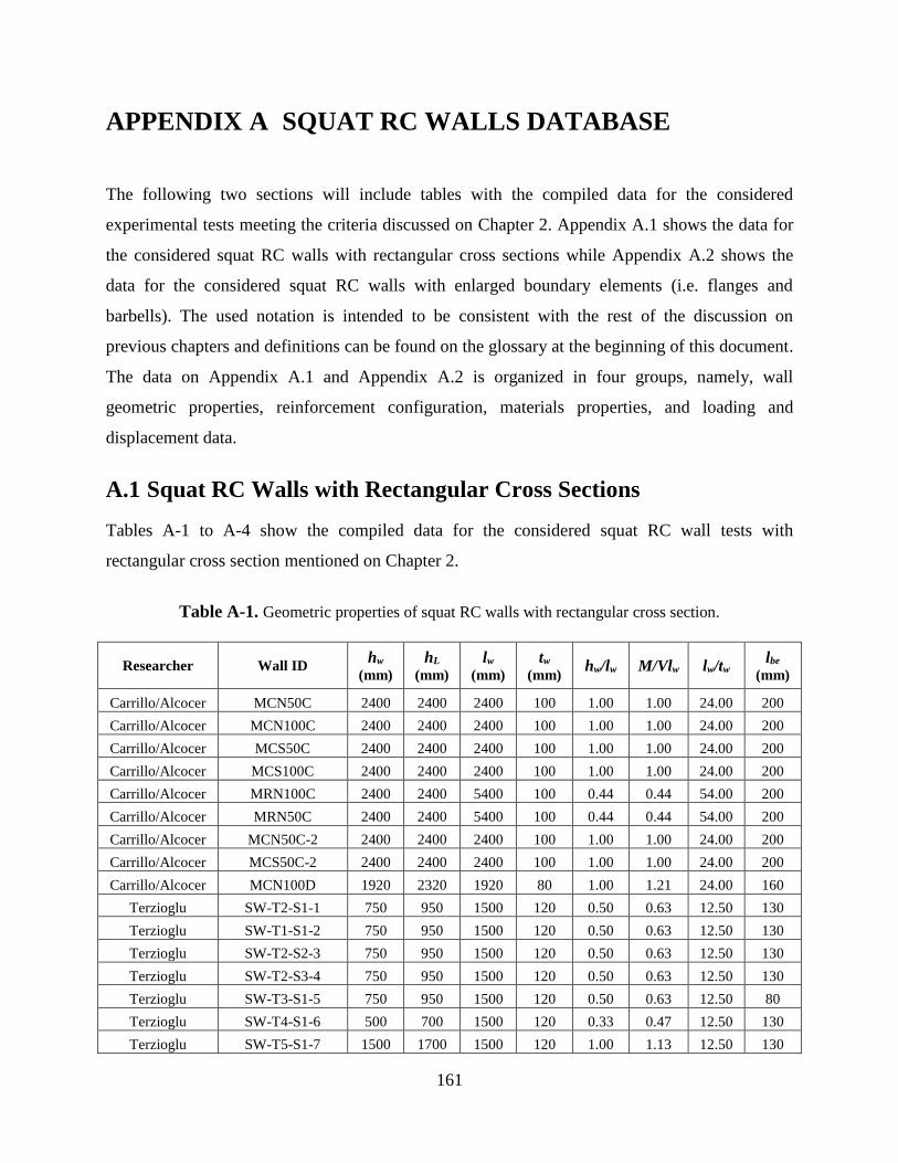
161

APPENDIX A SQUAT RC WALLS DATABASE

The following two sections will include tables with the compiled data for the considered

experimental tests meeting the criteria discussed on Chapter 2. Appendix A.1 shows the data for

the considered squat RC walls with rectangular cross sections while Appendix A.2 shows the

data for the considered squat RC walls with enlarged boundary elements (i.e. flanges and

barbells). The used notation is intended to be consistent with the rest of the discussion on

previous chapters and definitions can be found on the glossary at the beginning of this document.

The data on Appendix A.1 and Appendix A.2 is organized in four groups, namely, wall

geometric properties, reinforcement configuration, materials properties, and loading and

displacement data.

A.1 Squat RC Walls with Rectangular Cross Sections

Tables A-1 to A-4 show the compiled data for the considered squat RC wall tests with

rectangular cross section mentioned on Chapter 2.

Table A-1. Geometric properties of squat RC walls with rectangular cross section.

Researcher Wall ID hw

(mm)

hL (mm)

lw (mm)

tw

(mm) hw/lw M/Vlw lw/tw

lbe

(mm)

Carrillo/Alcocer MCN50C 2400 2400 2400 100 1.00 1.00 24.00 200

Carrillo/Alcocer MCN100C 2400 2400 2400 100 1.00 1.00 24.00 200

Carrillo/Alcocer MCS50C 2400 2400 2400 100 1.00 1.00 24.00 200

Carrillo/Alcocer MCS100C 2400 2400 2400 100 1.00 1.00 24.00 200

Carrillo/Alcocer MRN100C 2400 2400 5400 100 0.44 0.44 54.00 200

Carrillo/Alcocer MRN50C 2400 2400 5400 100 0.44 0.44 54.00 200

Carrillo/Alcocer MCN50C-2 2400 2400 2400 100 1.00 1.00 24.00 200

Carrillo/Alcocer MCS50C-2 2400 2400 2400 100 1.00 1.00 24.00 200

Carrillo/Alcocer MCN100D 1920 2320 1920 80 1.00 1.21 24.00 160

Terzioglu SW-T2-S1-1 750 950 1500 120 0.50 0.63 12.50 130

Terzioglu SW-T1-S1-2 750 950 1500 120 0.50 0.63 12.50 130

Terzioglu SW-T2-S2-3 750 950 1500 120 0.50 0.63 12.50 130

Terzioglu SW-T2-S3-4 750 950 1500 120 0.50 0.63 12.50 130

Terzioglu SW-T3-S1-5 750 950 1500 120 0.50 0.63 12.50 80

Terzioglu SW-T4-S1-6 500 700 1500 120 0.33 0.47 12.50 130

Terzioglu SW-T5-S1-7 1500 1700 1500 120 1.00 1.13 12.50 130

162


(mm)

hL (mm)

lw (mm)

tw


lbe

(mm)

Terzioglu SW-T6-S1-8 1500 1700 1500 120 1.00 1.13 12.50 130

Terzioglu SW-T1-S2-9 750 950 1500 120 0.50 0.63 12.50 130

Terzioglu SW-T1-N5-S1-10 750 950 1500 120 0.50 0.63 12.50 130

Terzioglu SW-T1-N10-S1-11 750 950 1500 120 0.50 0.63 12.50 130

NEES-UB SW1 2865 2865 3048 203 0.94 0.94 15.01 N/A

NEES-UB SW2 1646 1646 3048 203 0.54 0.54 15.01 N/A

NEES-UB SW3 1646 1646 3048 203 0.54 0.54 15.01 N/A

NEES-UB SW4 1646 1646 3048 203 0.54 0.54 15.01 N/A

NEES-UB SW5 1006 1006 3048 203 0.33 0.33 15.01 N/A

NEES-UB SW6 1006 1006 3048 203 0.33 0.33 15.01 N/A

NEES-UB SW7 1006 1006 3048 203 0.33 0.33 15.01 N/A

NEES-UB SW8 1646 1646 3048 203 0.54 0.54 15.01 N/A

NEES-UB SW9 1646 1646 3048 203 0.54 0.54 15.01 N/A

NEES-UB SW10 1646 1646 3048 203 0.54 0.54 15.01 N/A

NEES-UB SW11 1646 1646 3048 203 0.54 0.54 15.01 380

NEES-UB SW12 1646 1646 3048 203 0.54 0.54 15.01 380

Whyte Wall 1 1646 1646 3048 203 0.54 0.54 15.01 N/A

Whyte Wall 2 1646 1646 3048 203 0.54 0.54 15.01 N/A

Salonikios MSW3 1800 1925 1200 100 1.50 1.60 12.00 240

Salonikios MSW6 1800 1925 1200 100 1.50 1.60 12.00 240

Salonikios LSW1 1200 1325 1200 100 1.00 1.10 12.00 240

Salonikios LSW2 1200 1325 1200 100 1.00 1.10 12.00 240

Salonikios LSW3 1200 1325 1200 100 1.00 1.10 12.00 240

Wiradinata Wall 1 1000 1150 2000 100 0.50 0.58 20.00 320

Wiradinata Wall 2 500 650 2000 100 0.25 0.33 20.00 320

Pilette Wall4 1000 1160 2000 100 0.50 0.58 20.00 320

Pilette Wall 5 1000 1160 2000 100 0.50 0.58 20.00 250

M. Doostdar Wall 7 1500 1638 2000 100 0.75 0.82 20.00 320

M. Doostdar Wall 8 1500 1638 1500 100 1.00 1.09 15.00 360

Synge Wall 1 1500 1700 3000 100 0.50 0.57 30.00 200

Cardenas SW-13 1905 2057 1905 76 1.00 1.08 25.00 N/A

Greifenhagen M4 610 690 900 80 0.68 0.77 11.25 N/A

Park S1 1500 1750 1500 200 1.00 1.17 7.50 300

Park S2 1500 1750 1500 200 1.00 1.17 7.50 300

Park S3 1500 1750 1500 200 1.00 1.17 7.50 300

Park S5 1500 1750 1500 200 1.00 1.17 7.50 200

Park S6 1500 1750 1500 200 1.00 1.17 7.50 200

Park S7 1500 1750 1500 200 1.00 1.17 7.50 200

Hirosawa 72 1600 1700 1700 160 0.94 1.00 10.63 170

163


(mm)

hL (mm)

lw (mm)

tw


lbe

(mm)

Hirosawa 73 1600 1700 1700 160 0.94 1.00 10.63 170

Hirosawa 74 1600 1700 1700 160 0.94 1.00 10.63 170

Hirosawa 75 1600 1700 1700 160 0.94 1.00 10.63 170

Hirosawa 76 1600 1700 1700 160 0.94 1.00 10.63 170

Hirosawa 77 1600 1700 1700 160 0.94 1.00 10.63 170

Altin 1 1500 1650 1000 100 1.50 1.65 10.00 150

Alexander 1 1372 1372 2743 102 0.50 0.50 27.00 N/A

Rothe T10 1100 1200 800 80 1.38 1.50 10.00 150

Hwang/Sheu SWN-1D 500 650 1000 100 0.5 0.65 10 N/A

Hwang/Sheu SWN-5D 750 900 1000 100 0.75 0.9 10 N/A

Sheu SW-2 500 650 1000 100 0.5 0.65 10 N/A

Sheu SW-5 500 650 1000 100 0.5 0.65 10 N/A

Sheu SW-6 500 650 1000 100 0.5 0.65 10 N/A

Sheu SW-11 500 650 1000 100 0.5 0.65 10 N/A

Sheu SW-17 750 900 1000 100 0.75 0.9 10 N/A

N/A – Not Applicable

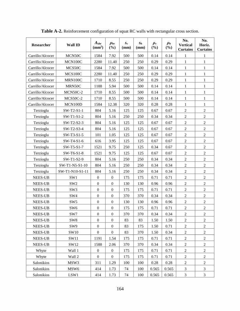
164

Table A-2. Reinforcement configuration of squat RC walls with rectangular cross section.

Researcher Wall ID Asbe

(mm2)

ρbe

(%)

sv (mm)

sh (mm)

ρv (%)

ρh (%)

No.

Vertical

Curtains

No.

Horiz.

Curtains

Carrillo/Alcocer MCN50C 1584 7.92 500 500 0.14 0.14 1 1

Carrillo/Alcocer MCN100C 2280 11.40 250 250 0.29 0.29 1 1

Carrillo/Alcocer MCS50C 1584 7.92 500 500 0.14 0.14 1 1

Carrillo/Alcocer MCS100C 2280 11.40 250 250 0.29 0.29 1 1

Carrillo/Alcocer MRN100C 1710 8.55 250 250 0.29 0.29 1 1

Carrillo/Alcocer MRN50C 1188 5.94 500 500 0.14 0.14 1 1

Carrillo/Alcocer MCN50C-2 1710 8.55 500 500 0.14 0.14 1 1

Carrillo/Alcocer MCS50C-2 1710 8.55 500 500 0.14 0.14 1 1

Carrillo/Alcocer MCN100D 1584 12.38 320 320 0.28 0.28 1 1

Terzioglu SW-T2-S1-1 804 5.16 125 125 0.67 0.67 2 2

Terzioglu SW-T1-S1-2 804 5.16 250 250 0.34 0.34 2 2

Terzioglu SW-T2-S2-3 804 5.16 125 125 0.67 0.67 2 2

Terzioglu SW-T2-S3-4 804 5.16 125 125 0.67 0.67 2 2

Terzioglu SW-T3-S1-5 101 1.05 125 125 0.67 0.67 2 2

Terzioglu SW-T4-S1-6 616 3.95 125 125 0.67 0.67 2 2

Terzioglu SW-T5-S1-7 1521 9.75 250 125 0.34 0.67 2 2

Terzioglu SW-T6-S1-8 1521 9.75 125 125 0.67 0.67 2 2

Terzioglu SW-T1-S2-9 804 5.16 250 250 0.34 0.34 2 2

Terzioglu SW-T1-N5-S1-10 804 5.16 250 250 0.34 0.34 2 2

Terzioglu SW-T1-N10-S1-11 804 5.16 250 250 0.34 0.34 2 2

NEES-UB SW1 0 0 175 175 0.71 0.71 2 2

NEES-UB SW2 0 0 130 130 0.96 0.96 2 2

NEES-UB SW3 0 0 175 175 0.71 0.71 2 2

NEES-UB SW4 0 0 370 370 0.34 0.34 2 2

NEES-UB SW5 0 0 130 130 0.96 0.96 2 2

NEES-UB SW6 0 0 175 175 0.71 0.71 2 2

NEES-UB SW7 0 0 370 370 0.34 0.34 2 2

NEES-UB SW8 0 0 83 83 1.50 1.50 2 2

NEES-UB SW9 0 0 83 175 1.50 0.71 2 2

NEES-UB SW10 0 0 83 370 1.50 0.34 2 2

NEES-UB SW11 1191 1.54 175 175 0.71 0.71 2 2

NEES-UB SW12 1588 2.06 370 370 0.34 0.34 2 2

Whyte Wall 1 0 0 175 175 0.71 0.71 2 2

Whyte Wall 2 0 0 175 175 0.71 0.71 2 2

Salonikios MSW3 311 1.29 100 100 0.28 0.28 2 2

Salonikios MSW6 414 1.73 74 100 0.565 0.565 3 3

Salonikios LSW1 414 1.73 74 100 0.565 0.565 3 3

165

Researcher Wall ID Asbe

(mm2)

ρbe

(%)

sv (mm)

sh (mm)

ρv (%)

ρh (%)

No.

Vertical

Curtains

No.

Horiz.

Curtains

Salonikios LSW2 311 1.29 100 100 0.28 0.28 2 2

Salonikios LSW3 311 1.29 100 100 0.28 0.28 2 2

Wiradinata Wall 1 401 1.25 284 300 0.71 0.21 2 2

Wiradinata Wall 2 401 1.25 284 300 0.71 0.21 2 2

Pilette Wall4 401 1.25 284 250 0.71 0.80 2 2

Pilette Wall 5 401 1.60 175 175 1.15 1.15 2 2

M. Doostdar Wall 7 401 1.25 284 250 0.71 0.80 2 2

M. Doostdar Wall 8 401 1.11 285 250 0.70 0.80 2 2

Synge Wall 1 452 2.26 140 120 0.81 1.68 1 1

Cardenas SW-13 0 0.00 89 95.3 2.93 0.98 1 1

Greifenhagen M4 0 0.00 219 122 0.32 0.26 2 2

Park S1 5819 9.70 300 250 0.66 0.51 2 2

Park S2 5819 9.70 300 180 0.66 0.70 2 2

Park S3 5819 9.70 300 250 0.66 0.51 2 2

Park S5 3879 9.70 550 500 0.36 0.25 2 2

Park S6 3879 9.70 550 500 0.36 0.25 2 2

Park S7 3879 9.70 550 500 0.36 0.25 2 2

Hirosawa 72 1546 5.68 132 264 0.52 0.26 2 2

Hirosawa 73 1546 5.68 132 264 0.52 0.26 2 2

Hirosawa 74 1546 5.68 132 132 0.52 0.52 2 2

Hirosawa 75 1546 5.68 132 132 0.52 0.52 2 2

Hirosawa 76 1546 5.68 132 66 0.52 1.04 2 2

Hirosawa 77 1546 5.68 132 66 0.52 1.04 2 2

Altin 1 1005 6.70 250 400 0.23 0.14 2 2

Alexander 1 0 0 114 114.3 0.30 0.30 1 1

Rothe T10 169 1.41 120 158 0.71 0.51 2 2

Hwang/Sheu SWN-1D 0 0 180 133 0.40 0.54 1 1

Hwang/Sheu SWN-5D 0 0 180 130 0.40 0.55 1 1

Sheu SW-2 0 0 180 133 0.40 0.54 1 1

Sheu SW-5 0 0 180 133 0.71 0.97 1 1

Sheu SW-6 0 0 180 133 0.71 0.97 1 1

Sheu SW-11 0 0 225 133 0.70 0.54 1 1

Sheu SW-17 0 0 225 130 0.70 0.55 1 1

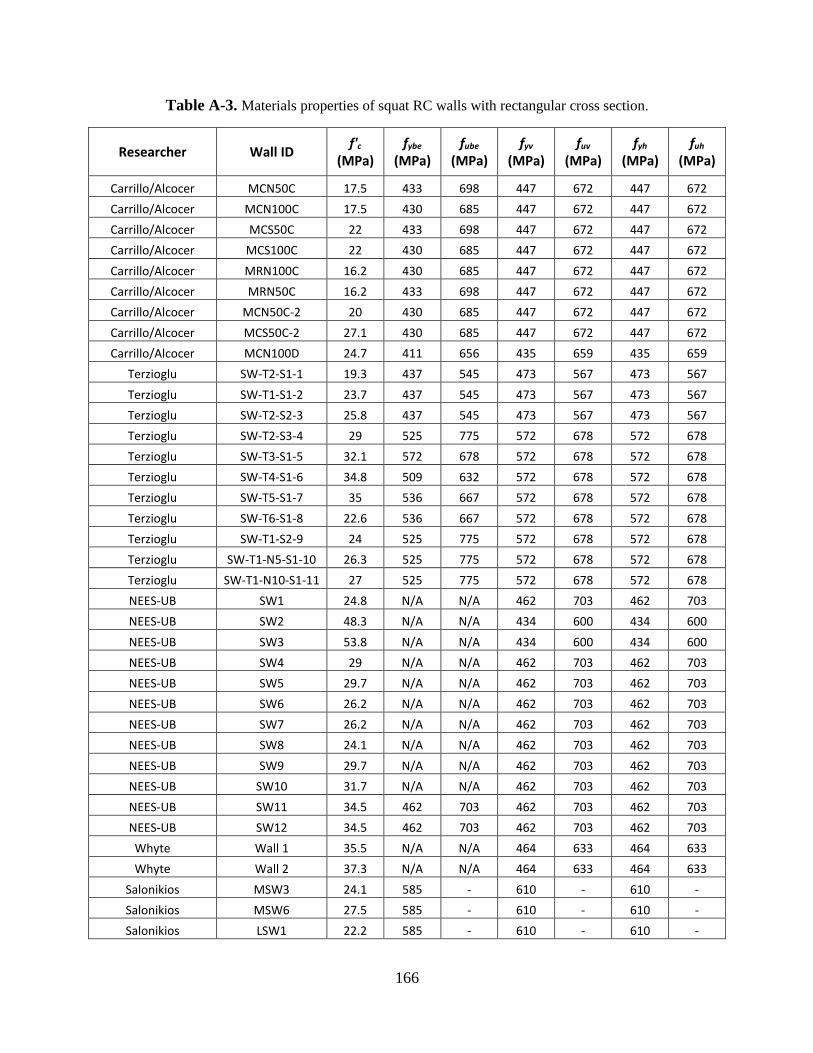
166

Table A-3. Materials properties of squat RC walls with rectangular cross section.

Researcher Wall ID f'c

(MPa) fybe

(MPa) fube

(MPa) fyv

(MPa) fuv

(MPa) fyh

(MPa) fuh

(MPa)

Carrillo/Alcocer MCN50C 17.5 433 698 447 672 447 672

Carrillo/Alcocer MCN100C 17.5 430 685 447 672 447 672

Carrillo/Alcocer MCS50C 22 433 698 447 672 447 672

Carrillo/Alcocer MCS100C 22 430 685 447 672 447 672

Carrillo/Alcocer MRN100C 16.2 430 685 447 672 447 672

Carrillo/Alcocer MRN50C 16.2 433 698 447 672 447 672

Carrillo/Alcocer MCN50C-2 20 430 685 447 672 447 672

Carrillo/Alcocer MCS50C-2 27.1 430 685 447 672 447 672

Carrillo/Alcocer MCN100D 24.7 411 656 435 659 435 659

Terzioglu SW-T2-S1-1 19.3 437 545 473 567 473 567

Terzioglu SW-T1-S1-2 23.7 437 545 473 567 473 567

Terzioglu SW-T2-S2-3 25.8 437 545 473 567 473 567

Terzioglu SW-T2-S3-4 29 525 775 572 678 572 678

Terzioglu SW-T3-S1-5 32.1 572 678 572 678 572 678

Terzioglu SW-T4-S1-6 34.8 509 632 572 678 572 678

Terzioglu SW-T5-S1-7 35 536 667 572 678 572 678

Terzioglu SW-T6-S1-8 22.6 536 667 572 678 572 678

Terzioglu SW-T1-S2-9 24 525 775 572 678 572 678

Terzioglu SW-T1-N5-S1-10 26.3 525 775 572 678 572 678

Terzioglu SW-T1-N10-S1-11 27 525 775 572 678 572 678

NEES-UB SW1 24.8 N/A N/A 462 703 462 703

NEES-UB SW2 48.3 N/A N/A 434 600 434 600

NEES-UB SW3 53.8 N/A N/A 434 600 434 600

NEES-UB SW4 29 N/A N/A 462 703 462 703

NEES-UB SW5 29.7 N/A N/A 462 703 462 703

NEES-UB SW6 26.2 N/A N/A 462 703 462 703

NEES-UB SW7 26.2 N/A N/A 462 703 462 703

NEES-UB SW8 24.1 N/A N/A 462 703 462 703

NEES-UB SW9 29.7 N/A N/A 462 703 462 703

NEES-UB SW10 31.7 N/A N/A 462 703 462 703

NEES-UB SW11 34.5 462 703 462 703 462 703

NEES-UB SW12 34.5 462 703 462 703 462 703

Whyte Wall 1 35.5 N/A N/A 464 633 464 633

Whyte Wall 2 37.3 N/A N/A 464 633 464 633

Salonikios MSW3 24.1 585 - 610 - 610 -

Salonikios MSW6 27.5 585 - 610 - 610 -

Salonikios LSW1 22.2 585 - 610 - 610 -

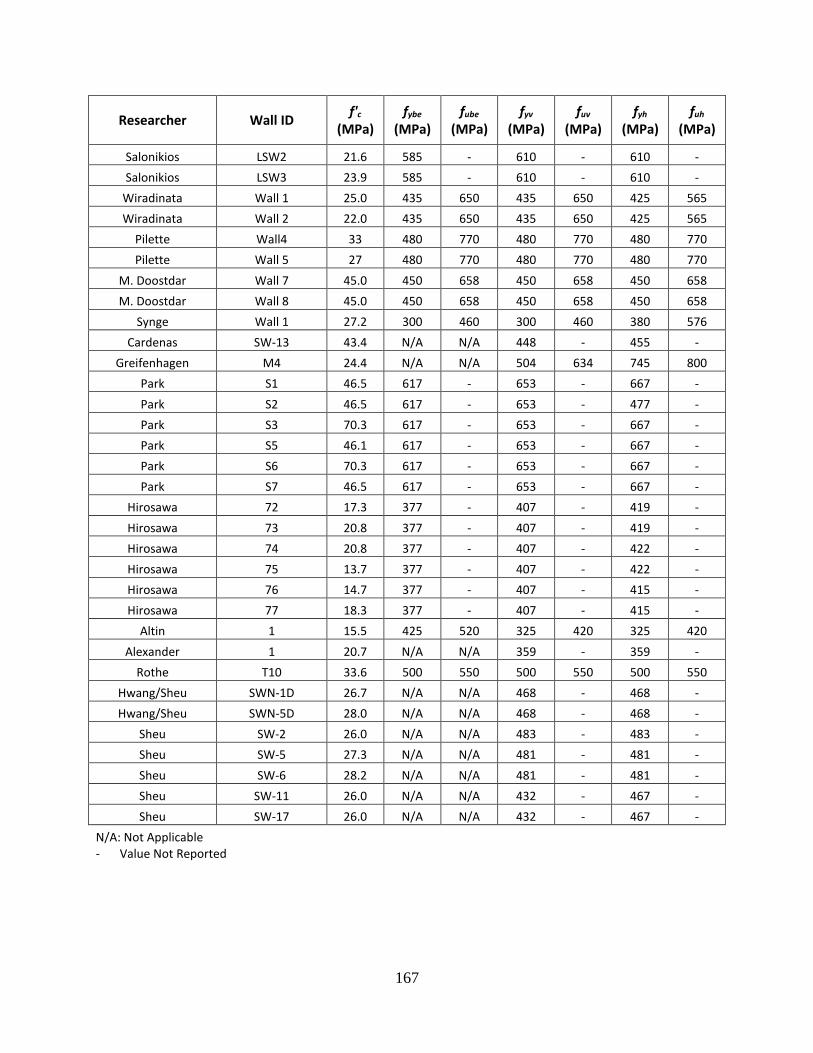
167

Researcher Wall ID f'c

(MPa) fybe

(MPa) fube

(MPa) fyv

(MPa) fuv

(MPa) fyh

(MPa) fuh

(MPa)

Salonikios LSW2 21.6 585 - 610 - 610 -

Salonikios LSW3 23.9 585 - 610 - 610 -

Wiradinata Wall 1 25.0 435 650 435 650 425 565

Wiradinata Wall 2 22.0 435 650 435 650 425 565

Pilette Wall4 33 480 770 480 770 480 770

Pilette Wall 5 27 480 770 480 770 480 770

M. Doostdar Wall 7 45.0 450 658 450 658 450 658

M. Doostdar Wall 8 45.0 450 658 450 658 450 658

Synge Wall 1 27.2 300 460 300 460 380 576

Cardenas SW-13 43.4 N/A N/A 448 - 455 -

Greifenhagen M4 24.4 N/A N/A 504 634 745 800

Park S1 46.5 617 - 653 - 667 -

Park S2 46.5 617 - 653 - 477 -

Park S3 70.3 617 - 653 - 667 -

Park S5 46.1 617 - 653 - 667 -

Park S6 70.3 617 - 653 - 667 -

Park S7 46.5 617 - 653 - 667 -

Hirosawa 72 17.3 377 - 407 - 419 -

Hirosawa 73 20.8 377 - 407 - 419 -

Hirosawa 74 20.8 377 - 407 - 422 -

Hirosawa 75 13.7 377 - 407 - 422 -

Hirosawa 76 14.7 377 - 407 - 415 -

Hirosawa 77 18.3 377 - 407 - 415 -

Altin 1 15.5 425 520 325 420 325 420

Alexander 1 20.7 N/A N/A 359 - 359 -

Rothe T10 33.6 500 550 500 550 500 550

Hwang/Sheu SWN-1D 26.7 N/A N/A 468 - 468 -

Hwang/Sheu SWN-5D 28.0 N/A N/A 468 - 468 -

Sheu SW-2 26.0 N/A N/A 483 - 483 -

Sheu SW-5 27.3 N/A N/A 481 - 481 -

Sheu SW-6 28.2 N/A N/A 481 - 481 -

Sheu SW-11 26.0 N/A N/A 432 - 467 -

Sheu SW-17 26.0 N/A N/A 432 - 467 -

N/A: Not Applicable - Value Not Reported

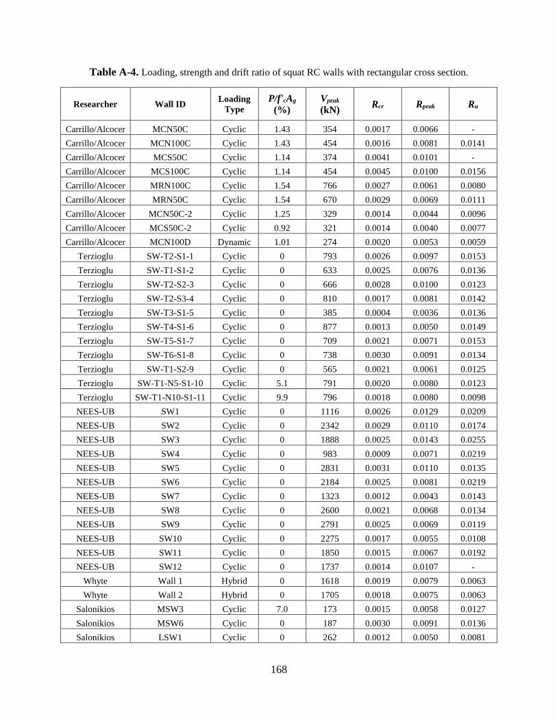
168

Table A-4. Loading, strength and drift ratio of squat RC walls with rectangular cross section.

Researcher Wall ID Loading

Type P/f'cAg

(%)

Vpeak

(kN) Rcr Rpeak Ru

Carrillo/Alcocer MCN50C Cyclic 1.43 354 0.0017 0.0066 -

Carrillo/Alcocer MCN100C Cyclic 1.43 454 0.0016 0.0081 0.0141

Carrillo/Alcocer MCS50C Cyclic 1.14 374 0.0041 0.0101 -

Carrillo/Alcocer MCS100C Cyclic 1.14 454 0.0045 0.0100 0.0156

Carrillo/Alcocer MRN100C Cyclic 1.54 766 0.0027 0.0061 0.0080

Carrillo/Alcocer MRN50C Cyclic 1.54 670 0.0029 0.0069 0.0111

Carrillo/Alcocer MCN50C-2 Cyclic 1.25 329 0.0014 0.0044 0.0096

Carrillo/Alcocer MCS50C-2 Cyclic 0.92 321 0.0014 0.0040 0.0077

Carrillo/Alcocer MCN100D Dynamic 1.01 274 0.0020 0.0053 0.0059

Terzioglu SW-T2-S1-1 Cyclic 0 793 0.0026 0.0097 0.0153









Terzioglu SW-T1-N5-S1-10 Cyclic 5.1 791 0.0020 0.0080 0.0123

Terzioglu SW-T1-N10-S1-11 Cyclic 9.9 796 0.0018 0.0080 0.0098

NEES-UB SW1 Cyclic 0 1116 0.0026 0.0129 0.0209

NEES-UB SW2 Cyclic 0 2342 0.0029 0.0110 0.0174

NEES-UB SW3 Cyclic 0 1888 0.0025 0.0143 0.0255

NEES-UB SW4 Cyclic 0 983 0.0009 0.0071 0.0219

NEES-UB SW5 Cyclic 0 2831 0.0031 0.0110 0.0135

NEES-UB SW6 Cyclic 0 2184 0.0025 0.0081 0.0219

NEES-UB SW7 Cyclic 0 1323 0.0012 0.0043 0.0143

NEES-UB SW8 Cyclic 0 2600 0.0021 0.0068 0.0134

NEES-UB SW9 Cyclic 0 2791 0.0025 0.0069 0.0119

NEES-UB SW10 Cyclic 0 2275 0.0017 0.0055 0.0108

NEES-UB SW11 Cyclic 0 1850 0.0015 0.0067 0.0192

NEES-UB SW12 Cyclic 0 1737 0.0014 0.0107 -

Whyte Wall 1 Hybrid 0 1618 0.0019 0.0079 0.0063

Whyte Wall 2 Hybrid 0 1705 0.0018 0.0075 0.0063

Salonikios MSW3 Cyclic 7.0 173 0.0015 0.0058 0.0127

Salonikios MSW6 Cyclic 0 187 0.0030 0.0091 0.0136

Salonikios LSW1 Cyclic 0 262 0.0012 0.0050 0.0081

169

Researcher Wall ID Loading

Type P/f'cAg

(%)

Vpeak

(kN) Rcr Rpeak Ru

Salonikios LSW2 Cyclic 0 185 0.0011 0.0044 0.0077

Salonikios LSW3 Cyclic 7.0 252 0.0008 0.0042 0.0115

Wiradinata Wall 1 Cyclic 0 531 0.0005 0.0079 0.0100

Wiradinata Wall 2 Cyclic 0 685 0.0006 0.0036 0.0120

Pilette Wall4 Cyclic 0 401 0.0019 0.0071 0.0204

Pilette Wall 5 Cyclic 0 545 0.0036 0.0140 0.0251

M. Doostdar Wall 7 Cyclic 0 375 0.0012 0.0050 0.0144

M. Doostdar Wall 8 Cyclic 0 225 0.0012 0.0089 0.0177

Synge Wall 1 Cyclic 0 774 0.0013 0.0044 0.0094

Cardenas SW-13 Cyclic 0 632 0.0022 0.0053 -

Greifenhagen M4 Cyclic 4.3 135 0.0007 0.0051 0.0186

Park S1 Cyclic 7.0 2158 0.0039 0.0101 0.0108

Park S2 Cyclic 7.0 2298 0.0041 0.0100 0.0119

Park S3 Cyclic 7.0 2085 0.0032 0.0082 0.0093

Park S5 Cyclic 7.0 1478 0.0023 0.0079 0.0102

Park S6 Cyclic 7.0 1876 0.0036 0.0095 0.0101

Park S7 Cyclic 7.0 1916 0.0035 0.0092 0.0112

Hirosawa 72 Cyclic 11.3 773 0.0012 0.0051 0.0096

Hirosawa 73 Cyclic 9.4 770 0.0011 0.0070 0.0080

Hirosawa 74 Cyclic 9.4 790 0.0011 0.0050 0.0091

Hirosawa 75 Cyclic 14.3 812 0.0013 0.0137 -

Hirosawa 76 Cyclic 13.4 791 0.0014 0.0052 0.0126

Hirosawa 77 Cyclic 10.7 875 0.0036 0.0099 -

Altin 1 Cyclic 0.0 146 0.0020 0.0056 0.0084

Alexander 1 Cyclic 0.0 329 - - -

Rothe T10 Cyclic 0.0 89 - - -

Hwang/Sheu SWN-1D Cyclic 12 323 0.0017 0.0063 0.0175

Hwang/Sheu SWN-5D Cyclic 12 247 0.0011 0.0097 -

Sheu SW-2 Cyclic 0 179 - - -





- Corresponding drift ratio value could not be obtained from the reported data.

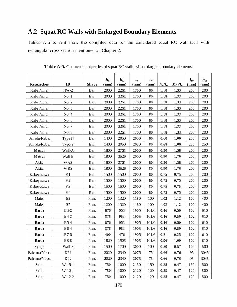
170

A.2 Squat RC Walls with Enlarged Boundary Elements

Tables A-5 to A-8 show the compiled data for the considered squat RC wall tests with

rectangular cross section mentioned on Chapter 2.

Table A-5. Geometric properties of squat RC walls with enlarged boundary elements.

Researcher ID Shape

hw (mm)

hL

(mm)

lw (mm)

tw (mm) hw/lw M/Vlw

lbe

(mm)

hbe (mm)

Kabe./Hira. NW-2 Bar. 2000 2261 1700 80 1.18 1.33 200 200

Kabe./Hira. No. 1 Bar. 2000 2261 1700 80 1.18 1.33 200 200

Kabe./Hira. No. 2 Bar. 2000 2261 1700 80 1.18 1.33 200 200

Kabe./Hira. No. 3 Bar. 2000 2261 1700 80 1.18 1.33 200 200

Kabe./Hira. No. 4 Bar. 2000 2261 1700 80 1.18 1.33 200 200

Kabe./Hira. No. 6 Bar. 2000 2261 1700 80 1.18 1.33 200 200

Kabe./Hira. No. 7 Bar. 2000 2261 1700 80 1.18 1.33 200 200

Kabe./Hira. No. 8 Bar. 2000 2261 1700 80 1.18 1.33 200 200

Sanada/Kabe. Type N Bar. 1400 2050 2050 80 0.68 1.00 250 250

Sanada/Kabe. Type S Bar. 1400 2050 2050 80 0.68 1.00 250 250

Matsui Wall-A Bar. 1800 2761 2000 80 0.90 1.38 200 200

Matsui Wall-B Bar. 1800 3526 2000 80 0.90 1.76 200 200

Akita WAS Bar. 1800 2761 2000 80 0.90 1.38 200 200

Akita WBS Bar. 1800 3526 2000 80 0.90 1.76 200 200

Kabeyasawa K1 Bar. 1500 1500 2000 80 0.75 0.75 200 200

Kabeyasawa K2 Bar. 1500 1500 2000 80 0.75 0.75 200 200

Kabeyasawa K3 Bar. 1500 1500 2000 80 0.75 0.75 200 200

Kabeyasawa K4 Bar. 1500 1500 2000 80 0.75 0.75 200 200

Maier S5 Flan. 1200 1320 1180 100 1.02 1.12 100 400

Maier S7 Flan. 1200 1320 1180 100 1.02 1.12 100 400

Barda B3-2 Flan. 876 953 1905 101.6 0.46 0.50 102 610

Barda B4-3 Flan. 876 953 1905 101.6 0.46 0.50 102 610

Barda B5-4 Flan. 876 953 1905 101.6 0.46 0.50 102 610

Barda B6-4 Flan. 876 953 1905 101.6 0.46 0.50 102 610

Barda B7-5 Flan. 400 476 1905 101.6 0.21 0.25 102 610

Barda B8-5 Flan. 1829 1905 1905 101.6 0.96 1.00 102 610

Synge Wall-3 Flan. 1500 1700 3000 100 0.50 0.57 100 500

Palermo/Vecc. DP1 Flan. 2020 2340 3075 75 0.66 0.76 95 3045

Palermo/Vecc. DP2 Flan. 2020 2340 3075 75 0.66 0.76 95 3045

Saito W-15-1 Flan. 750 1000 2150 150 0.35 0.47 150 500

Saito W-12-1 Flan. 750 1000 2120 120 0.35 0.47 120 500

Saito W-12-2 Flan. 750 1000 2120 120 0.35 0.47 120 500

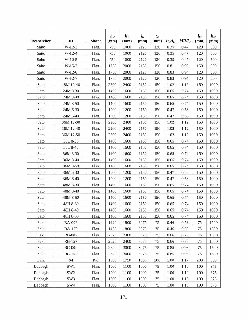
171

Researcher ID Shape

hw (mm)

hL

(mm)

lw (mm)

tw (mm) hw/lw M/Vlw

lbe

(mm)

hbe (mm)

Saito W-12-3 Flan. 750 1000 2120 120 0.35 0.47 120 500

Saito W-12-4 Flan. 750 1000 2120 120 0.35 0.47 120 500

Saito W-12-5 Flan. 750 1000 2120 120 0.35 0.47 120 500

Saito W-15-2 Flan. 1750 2000 2150 150 0.81 0.93 150 500

Saito W-12-6 Flan. 1750 2000 2120 120 0.83 0.94 120 500

Saito W-12-7 Flan. 1750 2000 2120 120 0.83 0.94 120 500

Sato 18M 12-40 Flan. 2200 2400 2150 150 1.02 1.12 150 1000

Sato 24M 8-30 Flan. 1400 1600 2150 150 0.65 0.74 150 1000

Sato 24M 8-40 Flan. 1400 1600 2150 150 0.65 0.74 150 1000

Sato 24M 8-50 Flan. 1400 1600 2150 150 0.65 0.74 150 1000

Sato 24M 6-30 Flan. 1000 1200 2150 150 0.47 0.56 150 1000

Sato 24M 6-40 Flan. 1000 1200 2150 150 0.47 0.56 150 1000

Sato 36M 12-30 Flan. 2200 2400 2150 150 1.02 1.12 150 1000

Sato 36M 12-40 Flan. 2200 2400 2150 150 1.02 1.12 150 1000

Sato 36M 12-50 Flan. 2200 2400 2150 150 1.02 1.12 150 1000

Sato 36L 8-30 Flan. 1400 1600 2150 150 0.65 0.74 150 1000

Sato 36L 8-40 Flan. 1400 1600 2150 150 0.65 0.74 150 1000

Sato 36M 8-30 Flan. 1400 1600 2150 150 0.65 0.74 150 1000

Sato 36M 8-40 Flan. 1400 1600 2150 150 0.65 0.74 150 1000

Sato 36M 8-50 Flan. 1400 1600 2150 150 0.65 0.74 150 1000

Sato 36M 6-30 Flan. 1000 1200 2150 150 0.47 0.56 150 1000

Sato 36M 6-40 Flan. 1000 1200 2150 150 0.47 0.56 150 1000

Sato 48M 8-30 Flan. 1400 1600 2150 150 0.65 0.74 150 1000

Sato 48M 8-40 Flan. 1400 1600 2150 150 0.65 0.74 150 1000

Sato 48M 8-50 Flan. 1400 1600 2150 150 0.65 0.74 150 1000

Sato 48H 8-30 Flan. 1400 1600 2150 150 0.65 0.74 150 1000

Sato 48H 8-40 Flan. 1400 1600 2150 150 0.65 0.74 150 1000

Sato 48H 8-50 Flan. 1400 1600 2150 150 0.65 0.74 150 1000

Seki RA-00P Flan. 1420 1800 3075 75 0.46 0.59 75 1500

Seki RA-15P Flan. 1420 1800 3075 75 0.46 0.59 75 1500

Seki RB-00P Flan. 2020 2400 3075 75 0.66 0.78 75 1500

Seki RB-15P Flan. 2020 2400 3075 75 0.66 0.78 75 1500

Seki RC-00P Flan. 2620 3000 3075 75 0.85 0.98 75 1500

Seki RC-15P Flan. 2620 3000 3075 75 0.85 0.98 75 1500

Park S4 Bar. 1500 1750 1500 200 1.00 1.17 200 300

Dabbagh SW1 Flan. 1000 1100 1000 75 1.00 1.10 100 375

Dabbagh SW2 Flan. 1000 1100 1000 75 1.00 1.10 100 375

Dabbagh SW3 Flan. 1000 1100 1000 75 1.00 1.10 100 375

Dabbagh SW4 Flan. 1000 1100 1000 75 1.00 1.10 100 375

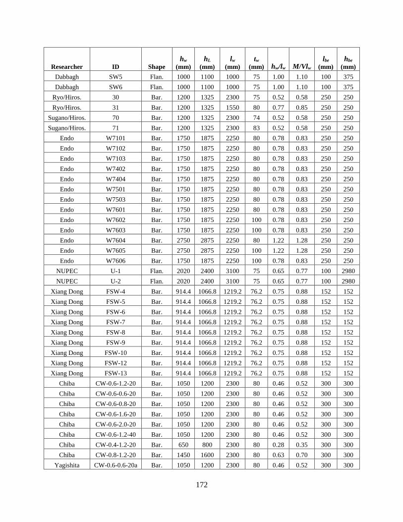
172

Researcher ID Shape

hw (mm)

hL

(mm)

lw (mm)

tw (mm) hw/lw M/Vlw

lbe

(mm)

hbe (mm)

Dabbagh SW5 Flan. 1000 1100 1000 75 1.00 1.10 100 375

Dabbagh SW6 Flan. 1000 1100 1000 75 1.00 1.10 100 375

Ryo/Hiros. 30 Bar. 1200 1325 2300 75 0.52 0.58 250 250

Ryo/Hiros. 31 Bar. 1200 1325 1550 80 0.77 0.85 250 250

Sugano/Hiros. 70 Bar. 1200 1325 2300 74 0.52 0.58 250 250

Sugano/Hiros. 71 Bar. 1200 1325 2300 83 0.52 0.58 250 250

Endo W7101 Bar. 1750 1875 2250 80 0.78 0.83 250 250

Endo W7102 Bar. 1750 1875 2250 80 0.78 0.83 250 250

Endo W7103 Bar. 1750 1875 2250 80 0.78 0.83 250 250

Endo W7402 Bar. 1750 1875 2250 80 0.78 0.83 250 250

Endo W7404 Bar. 1750 1875 2250 80 0.78 0.83 250 250

Endo W7501 Bar. 1750 1875 2250 80 0.78 0.83 250 250

Endo W7503 Bar. 1750 1875 2250 80 0.78 0.83 250 250

Endo W7601 Bar. 1750 1875 2250 80 0.78 0.83 250 250

Endo W7602 Bar. 1750 1875 2250 100 0.78 0.83 250 250

Endo W7603 Bar. 1750 1875 2250 100 0.78 0.83 250 250

Endo W7604 Bar. 2750 2875 2250 80 1.22 1.28 250 250

Endo W7605 Bar. 2750 2875 2250 100 1.22 1.28 250 250

Endo W7606 Bar. 1750 1875 2250 100 0.78 0.83 250 250

NUPEC U-1 Flan. 2020 2400 3100 75 0.65 0.77 100 2980

NUPEC U-2 Flan. 2020 2400 3100 75 0.65 0.77 100 2980

Xiang Dong FSW-4 Bar. 914.4 1066.8 1219.2 76.2 0.75 0.88 152 152









Chiba CW-0.6-1.2-20 Bar. 1050 1200 2300 80 0.46 0.52 300 300

Chiba CW-0.6-0.6-20 Bar. 1050 1200 2300 80 0.46 0.52 300 300

Chiba CW-0.6-0.8-20 Bar. 1050 1200 2300 80 0.46 0.52 300 300

Chiba CW-0.6-1.6-20 Bar. 1050 1200 2300 80 0.46 0.52 300 300

Chiba CW-0.6-2.0-20 Bar. 1050 1200 2300 80 0.46 0.52 300 300

Chiba CW-0.6-1.2-40 Bar. 1050 1200 2300 80 0.46 0.52 300 300

Chiba CW-0.4-1.2-20 Bar. 650 800 2300 80 0.28 0.35 300 300

Chiba CW-0.8-1.2-20 Bar. 1450 1600 2300 80 0.63 0.70 300 300

Yagishita CW-0.6-0.6-20a Bar. 1050 1200 2300 80 0.46 0.52 300 300

173

Researcher ID Shape

hw (mm)

hL

(mm)

lw (mm)

tw (mm) hw/lw M/Vlw

lbe

(mm)

hbe (mm)

Yagishita CW-0.6-0.8-20a Bar. 1050 1200 2300 80 0.46 0.52 300 300

Yagishita CW-0.6-1.2-0 Bar. 1050 1200 2300 80 0.46 0.52 300 300

Fukuzawa CW-0.6-0-20 Bar. 1050 1200 2300 80 0.46 0.52 300 300

Fukuzawa CW-0.6-0.3-20 Bar. 1050 1200 2300 80 0.46 0.52 300 300

Fukuzawa CW-0.6-2.4-20 Bar. 1050 1200 2300 80 0.46 0.52 300 300

Fukuzawa CW-0.6-2.8-20 Bar. 1050 1200 2300 80 0.46 0.52 300 300

Fukuzawa CW-0.6-0-0 Bar. 1050 1200 2300 80 0.46 0.52 300 300

Fukuzawa CW-0.6-0-40 Bar. 1050 1200 2300 80 0.46 0.52 300 300

Fukuzawa CW-0.6-0.6-0 Bar. 1050 1200 2300 80 0.46 0.52 300 300

Fukuzawa CW-0.6-0.6-40 Bar. 1050 1200 2300 80 0.46 0.52 300 300

Fukuzawa CW-0.4-0.6-20 Bar. 650 800 2300 80 0.28 0.35 300 300

Fukuzawa CW-0.8-0.6-20 Bar. 1450 1600 2300 80 0.63 0.70 300 300

Fukuzawa CW-0.4-2.0-20 Bar. 650 800 2300 80 0.28 0.35 300 300

Fukuzawa CW-0.8-2.0-20 Bar. 1450 1600 2300 80 0.63 0.70 300 300

Hatori CW-0.6-2-0 Bar. 1050 1200 2300 80 0.46 0.52 300 300

Hatori CW-0.6-2-40 Bar. 1050 1200 2300 80 0.46 0.52 300 300

Hatori CW-0.6-2-20B Bar. 1050 1200 2300 80 0.46 0.52 300 300

Hatori CW-0.6-0.6-20L Bar. 1050 1200 2300 80 0.46 0.52 300 300

Hatori CW-0.6-1.2-20L Bar. 1050 1200 2300 80 0.46 0.52 300 300

Hatori CW-0.6-2-20L Bar. 1050 1200 2300 80 0.46 0.52 300 300

Taga No 1 Bar. 1050 1200 2180 80 0.48 0.55 180 180

Taga No 2 Bar. 1050 1200 2180 80 0.48 0.55 180 180

Taga No 3 Bar. 1050 1200 2180 80 0.48 0.55 180 180

Taga No 4 Bar. 1050 1200 2180 80 0.48 0.55 180 180

Taga No 5 Bar. 1050 1200 2180 80 0.48 0.55 180 180

Taga No 6 Bar. 1050 1200 2180 80 0.48 0.55 180 180

Bar. – Barbell cross section

Flan. – Flanged cross section

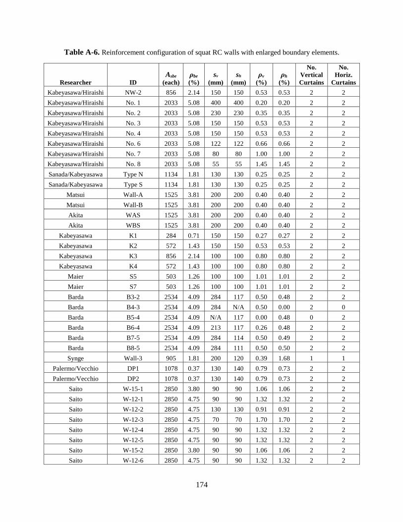
174

Table A-6. Reinforcement configuration of squat RC walls with enlarged boundary elements.

Researcher ID

Asbe

(each)

ρbe

(%)

sv

(mm)

sh

(mm)

ρv

(%)

ρh

(%)

No.

Vertical

Curtains

No.

Horiz.

Curtains

Kabeyasawa/Hiraishi NW-2 856 2.14 150 150 0.53 0.53 2 2

Kabeyasawa/Hiraishi No. 1 2033 5.08 400 400 0.20 0.20 2 2







Sanada/Kabeyasawa Type N 1134 1.81 130 130 0.25 0.25 2 2

Sanada/Kabeyasawa Type S 1134 1.81 130 130 0.25 0.25 2 2

Matsui Wall-A 1525 3.81 200 200 0.40 0.40 2 2

Matsui Wall-B 1525 3.81 200 200 0.40 0.40 2 2

Akita WAS 1525 3.81 200 200 0.40 0.40 2 2

Akita WBS 1525 3.81 200 200 0.40 0.40 2 2

Kabeyasawa K1 284 0.71 150 150 0.27 0.27 2 2

Kabeyasawa K2 572 1.43 150 150 0.53 0.53 2 2

Kabeyasawa K3 856 2.14 100 100 0.80 0.80 2 2

Kabeyasawa K4 572 1.43 100 100 0.80 0.80 2 2

Maier S5 503 1.26 100 100 1.01 1.01 2 2

Maier S7 503 1.26 100 100 1.01 1.01 2 2

Barda B3-2 2534 4.09 284 117 0.50 0.48 2 2

Barda B4-3 2534 4.09 284 N/A 0.50 0.00 2 0

Barda B5-4 2534 4.09 N/A 117 0.00 0.48 0 2

Barda B6-4 2534 4.09 213 117 0.26 0.48 2 2

Barda B7-5 2534 4.09 284 114 0.50 0.49 2 2

Barda B8-5 2534 4.09 284 111 0.50 0.50 2 2

Synge Wall-3 905 1.81 200 120 0.39 1.68 1 1

Palermo/Vecchio DP1 1078 0.37 130 140 0.79 0.73 2 2

Palermo/Vecchio DP2 1078 0.37 130 140 0.79 0.73 2 2

Saito W-15-1 2850 3.80 90 90 1.06 1.06 2 2

Saito W-12-1 2850 4.75 90 90 1.32 1.32 2 2

Saito W-12-2 2850 4.75 130 130 0.91 0.91 2 2

Saito W-12-3 2850 4.75 70 70 1.70 1.70 2 2

Saito W-12-4 2850 4.75 90 90 1.32 1.32 2 2

Saito W-12-5 2850 4.75 90 90 1.32 1.32 2 2

Saito W-15-2 2850 3.80 90 90 1.06 1.06 2 2

Saito W-12-6 2850 4.75 90 90 1.32 1.32 2 2

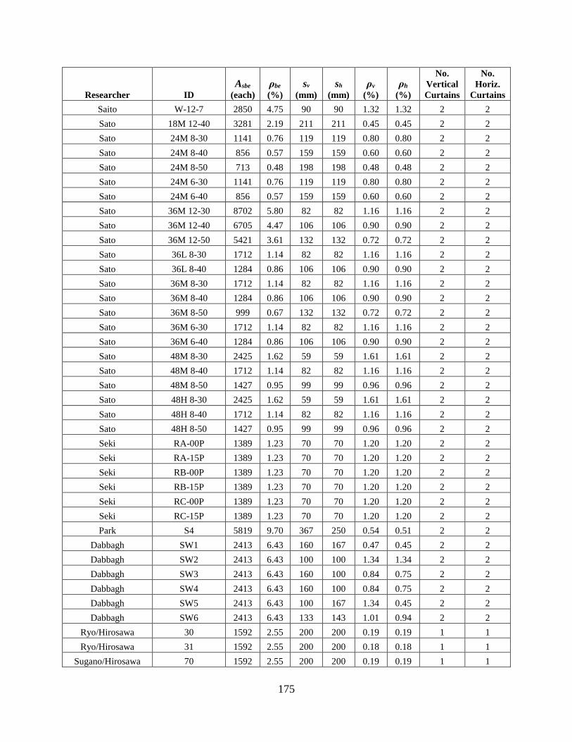
175

Researcher ID

Asbe

(each)

ρbe

(%)

sv

(mm)

sh

(mm)

ρv

(%)

ρh

(%)

No.

Vertical

Curtains

No.

Horiz.

Curtains

Saito W-12-7 2850 4.75 90 90 1.32 1.32 2 2

Sato 18M 12-40 3281 2.19 211 211 0.45 0.45 2 2

Sato 24M 8-30 1141 0.76 119 119 0.80 0.80 2 2

Sato 24M 8-40 856 0.57 159 159 0.60 0.60 2 2

Sato 24M 8-50 713 0.48 198 198 0.48 0.48 2 2

Sato 24M 6-30 1141 0.76 119 119 0.80 0.80 2 2

Sato 24M 6-40 856 0.57 159 159 0.60 0.60 2 2

Sato 36M 12-30 8702 5.80 82 82 1.16 1.16 2 2

Sato 36M 12-40 6705 4.47 106 106 0.90 0.90 2 2

Sato 36M 12-50 5421 3.61 132 132 0.72 0.72 2 2

Sato 36L 8-30 1712 1.14 82 82 1.16 1.16 2 2

Sato 36L 8-40 1284 0.86 106 106 0.90 0.90 2 2

Sato 36M 8-30 1712 1.14 82 82 1.16 1.16 2 2

Sato 36M 8-40 1284 0.86 106 106 0.90 0.90 2 2

Sato 36M 8-50 999 0.67 132 132 0.72 0.72 2 2

Sato 36M 6-30 1712 1.14 82 82 1.16 1.16 2 2

Sato 36M 6-40 1284 0.86 106 106 0.90 0.90 2 2

Sato 48M 8-30 2425 1.62 59 59 1.61 1.61 2 2

Sato 48M 8-40 1712 1.14 82 82 1.16 1.16 2 2

Sato 48M 8-50 1427 0.95 99 99 0.96 0.96 2 2

Sato 48H 8-30 2425 1.62 59 59 1.61 1.61 2 2

Sato 48H 8-40 1712 1.14 82 82 1.16 1.16 2 2

Sato 48H 8-50 1427 0.95 99 99 0.96 0.96 2 2

Seki RA-00P 1389 1.23 70 70 1.20 1.20 2 2

Seki RA-15P 1389 1.23 70 70 1.20 1.20 2 2

Seki RB-00P 1389 1.23 70 70 1.20 1.20 2 2

Seki RB-15P 1389 1.23 70 70 1.20 1.20 2 2

Seki RC-00P 1389 1.23 70 70 1.20 1.20 2 2

Seki RC-15P 1389 1.23 70 70 1.20 1.20 2 2

Park S4 5819 9.70 367 250 0.54 0.51 2 2

Dabbagh SW1 2413 6.43 160 167 0.47 0.45 2 2

Dabbagh SW2 2413 6.43 100 100 1.34 1.34 2 2

Dabbagh SW3 2413 6.43 160 100 0.84 0.75 2 2

Dabbagh SW4 2413 6.43 160 100 0.84 0.75 2 2

Dabbagh SW5 2413 6.43 100 167 1.34 0.45 2 2

Dabbagh SW6 2413 6.43 133 143 1.01 0.94 2 2

Ryo/Hirosawa 30 1592 2.55 200 200 0.19 0.19 1 1

Ryo/Hirosawa 31 1592 2.55 200 200 0.18 0.18 1 1

Sugano/Hirosawa 70 1592 2.55 200 200 0.19 0.19 1 1

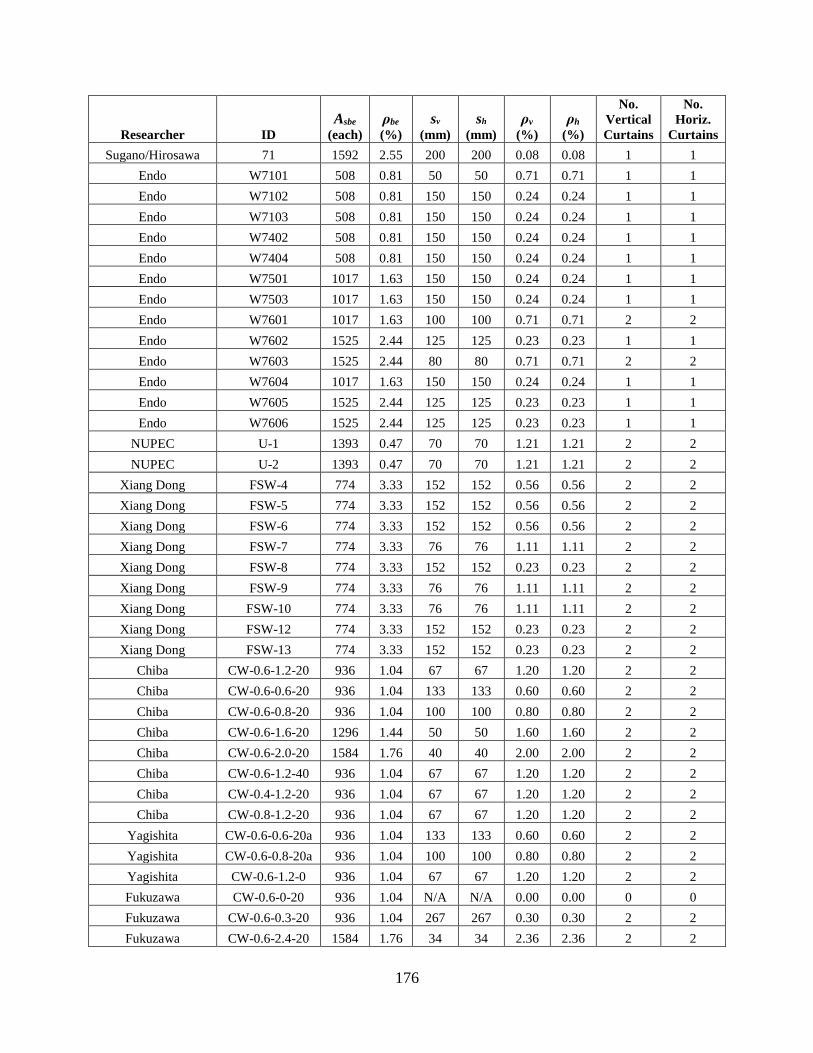
176

Researcher ID

Asbe

(each)

ρbe

(%)

sv

(mm)

sh

(mm)

ρv

(%)

ρh

(%)

No.

Vertical

Curtains

No.

Horiz.

Curtains

Sugano/Hirosawa 71 1592 2.55 200 200 0.08 0.08 1 1

Endo W7101 508 0.81 50 50 0.71 0.71 1 1

Endo W7102 508 0.81 150 150 0.24 0.24 1 1

Endo W7103 508 0.81 150 150 0.24 0.24 1 1

Endo W7402 508 0.81 150 150 0.24 0.24 1 1

Endo W7404 508 0.81 150 150 0.24 0.24 1 1

Endo W7501 1017 1.63 150 150 0.24 0.24 1 1

Endo W7503 1017 1.63 150 150 0.24 0.24 1 1

Endo W7601 1017 1.63 100 100 0.71 0.71 2 2

Endo W7602 1525 2.44 125 125 0.23 0.23 1 1

Endo W7603 1525 2.44 80 80 0.71 0.71 2 2

Endo W7604 1017 1.63 150 150 0.24 0.24 1 1

Endo W7605 1525 2.44 125 125 0.23 0.23 1 1

Endo W7606 1525 2.44 125 125 0.23 0.23 1 1

NUPEC U-1 1393 0.47 70 70 1.21 1.21 2 2

NUPEC U-2 1393 0.47 70 70 1.21 1.21 2 2

Xiang Dong FSW-4 774 3.33 152 152 0.56 0.56 2 2

Xiang Dong FSW-5 774 3.33 152 152 0.56 0.56 2 2

Xiang Dong FSW-6 774 3.33 152 152 0.56 0.56 2 2

Xiang Dong FSW-7 774 3.33 76 76 1.11 1.11 2 2

Xiang Dong FSW-8 774 3.33 152 152 0.23 0.23 2 2

Xiang Dong FSW-9 774 3.33 76 76 1.11 1.11 2 2

Xiang Dong FSW-10 774 3.33 76 76 1.11 1.11 2 2

Xiang Dong FSW-12 774 3.33 152 152 0.23 0.23 2 2

Xiang Dong FSW-13 774 3.33 152 152 0.23 0.23 2 2

Chiba CW-0.6-1.2-20 936 1.04 67 67 1.20 1.20 2 2

Chiba CW-0.6-0.6-20 936 1.04 133 133 0.60 0.60 2 2

Chiba CW-0.6-0.8-20 936 1.04 100 100 0.80 0.80 2 2

Chiba CW-0.6-1.6-20 1296 1.44 50 50 1.60 1.60 2 2

Chiba CW-0.6-2.0-20 1584 1.76 40 40 2.00 2.00 2 2

Chiba CW-0.6-1.2-40 936 1.04 67 67 1.20 1.20 2 2

Chiba CW-0.4-1.2-20 936 1.04 67 67 1.20 1.20 2 2

Chiba CW-0.8-1.2-20 936 1.04 67 67 1.20 1.20 2 2

Yagishita CW-0.6-0.6-20a 936 1.04 133 133 0.60 0.60 2 2

Yagishita CW-0.6-0.8-20a 936 1.04 100 100 0.80 0.80 2 2

Yagishita CW-0.6-1.2-0 936 1.04 67 67 1.20 1.20 2 2

Fukuzawa CW-0.6-0-20 936 1.04 N/A N/A 0.00 0.00 0 0

Fukuzawa CW-0.6-0.3-20 936 1.04 267 267 0.30 0.30 2 2

Fukuzawa CW-0.6-2.4-20 1584 1.76 34 34 2.36 2.36 2 2

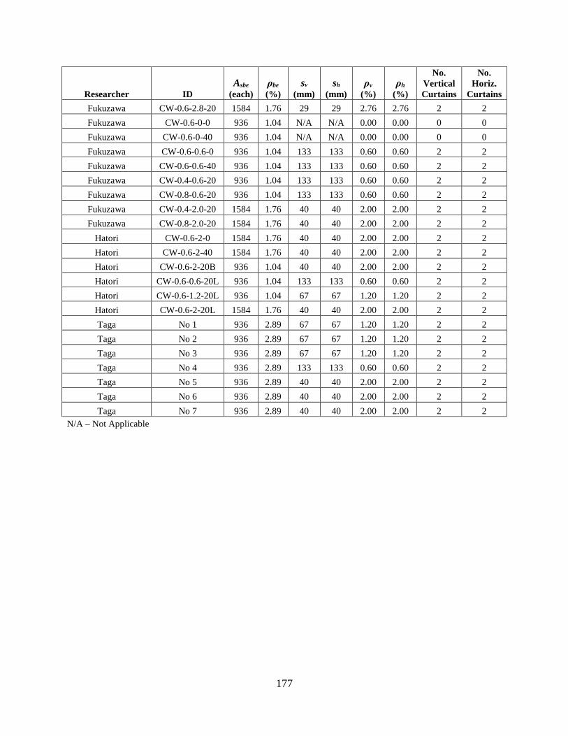
177

Researcher ID

Asbe

(each)

ρbe

(%)

sv

(mm)

sh

(mm)

ρv

(%)

ρh

(%)

No.

Vertical

Curtains

No.

Horiz.

Curtains

Fukuzawa CW-0.6-2.8-20 1584 1.76 29 29 2.76 2.76 2 2

Fukuzawa CW-0.6-0-0 936 1.04 N/A N/A 0.00 0.00 0 0

Fukuzawa CW-0.6-0-40 936 1.04 N/A N/A 0.00 0.00 0 0

Fukuzawa CW-0.6-0.6-0 936 1.04 133 133 0.60 0.60 2 2

Fukuzawa CW-0.6-0.6-40 936 1.04 133 133 0.60 0.60 2 2

Fukuzawa CW-0.4-0.6-20 936 1.04 133 133 0.60 0.60 2 2

Fukuzawa CW-0.8-0.6-20 936 1.04 133 133 0.60 0.60 2 2

Fukuzawa CW-0.4-2.0-20 1584 1.76 40 40 2.00 2.00 2 2

Fukuzawa CW-0.8-2.0-20 1584 1.76 40 40 2.00 2.00 2 2

Hatori CW-0.6-2-0 1584 1.76 40 40 2.00 2.00 2 2

Hatori CW-0.6-2-40 1584 1.76 40 40 2.00 2.00 2 2

Hatori CW-0.6-2-20B 936 1.04 40 40 2.00 2.00 2 2

Hatori CW-0.6-0.6-20L 936 1.04 133 133 0.60 0.60 2 2

Hatori CW-0.6-1.2-20L 936 1.04 67 67 1.20 1.20 2 2

Hatori CW-0.6-2-20L 1584 1.76 40 40 2.00 2.00 2 2

Taga No 1 936 2.89 67 67 1.20 1.20 2 2

Taga No 2 936 2.89 67 67 1.20 1.20 2 2

Taga No 3 936 2.89 67 67 1.20 1.20 2 2

Taga No 4 936 2.89 133 133 0.60 0.60 2 2

Taga No 5 936 2.89 40 40 2.00 2.00 2 2

Taga No 6 936 2.89 40 40 2.00 2.00 2 2

Taga No 7 936 2.89 40 40 2.00 2.00 2 2

N/A – Not Applicable

178

Table A-7. Material properties of squat RC walls with enlarged boundary elements.

Researcher ID

f'c

( MPa)

fybe

(MPa)

fube

(MPa)

fyv

(MPa)

fuv

(MPa)

fyh

(MPa)

fuh

(MPa)

Kabeyasawa/Hiraishi NW-2 93.6 776 968 1001 1128 1001 1128

Kabeyasawa/Hiraishi No. 1 65.1 1009 - 792 - 792 -







Sanada/Kabeyasawa Type N 22.4 398 557 340 560 340 560

Sanada/Kabeyasawa Type S 24.5 398 557 340 560 340 560

Matsui Wall-A 28.2 434 605 377 493 377 493

Matsui Wall-B 27.4 434 605 377 493 377 493

Akita WAS 27 434 605 377 493 377 493

Akita WBS 27 434 605 377 493 377 493

Kabeyasawa K1 19.2 392 557 395 526 395 526

Kabeyasawa K2 19.2 392 557 395 526 395 526

Kabeyasawa K3 19.2 392 557 395 526 395 526

Kabeyasawa K4 20.8 392 557 395 526 395 526

Maier S5 37.3 574 - 574 - 574 -

Maier S7 34.1 555 - 555 - 555 -

Barda B3-2 27.0 414 667 545 850 513 672

Barda B4-3 19.0 527 808 535 825 N/A N/A

Barda B5-4 28.9 527 807 N/A N/A 495 678

Barda B6-4 21.2 529 802 496 654 496 654

Barda B7-5 25.7 539 794 531 830 501 662

Barda B8-5 23.4 489 778 527 755 496 675

Synge Wall-3 26 300 460 315 440 380 576

Palermo/Vecchio DP1 21.7 605 652 605 652 605 652

Palermo/Vecchio DP2 18.8 605 652 605 652 605 652

Saito W-15-1 24.8 369 526 369 526 369 526

Saito W-12-1 35.2 369 526 369 526 369 526

Saito W-12-2 38.1 369 526 369 526 369 526

Saito W-12-3 35.8 369 526 369 526 369 526

Saito W-12-4 35.8 369 526 369 526 369 526

Saito W-12-5 40.4 369 526 369 526 369 526

Saito W-15-2 25.9 369 526 369 526 369 526

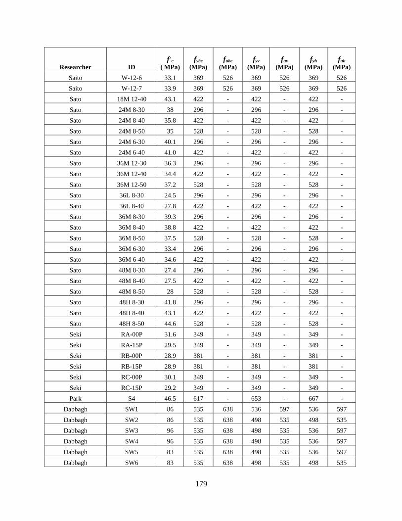
179

Researcher ID

f'c

( MPa)

fybe

(MPa)

fube

(MPa)

fyv

(MPa)

fuv

(MPa)

fyh

(MPa)

fuh

(MPa)

Saito W-12-6 33.1 369 526 369 526 369 526

Saito W-12-7 33.9 369 526 369 526 369 526

Sato 18M 12-40 43.1 422 - 422 - 422 -

Sato 24M 8-30 38 296 - 296 - 296 -

Sato 24M 8-40 35.8 422 - 422 - 422 -

Sato 24M 8-50 35 528 - 528 - 528 -

Sato 24M 6-30 40.1 296 - 296 - 296 -

Sato 24M 6-40 41.0 422 - 422 - 422 -

Sato 36M 12-30 36.3 296 - 296 - 296 -

Sato 36M 12-40 34.4 422 - 422 - 422 -

Sato 36M 12-50 37.2 528 - 528 - 528 -

Sato 36L 8-30 24.5 296 - 296 - 296 -

Sato 36L 8-40 27.8 422 - 422 - 422 -

Sato 36M 8-30 39.3 296 - 296 - 296 -

Sato 36M 8-40 38.8 422 - 422 - 422 -

Sato 36M 8-50 37.5 528 - 528 - 528 -

Sato 36M 6-30 33.4 296 - 296 - 296 -

Sato 36M 6-40 34.6 422 - 422 - 422 -

Sato 48M 8-30 27.4 296 - 296 - 296 -

Sato 48M 8-40 27.5 422 - 422 - 422 -

Sato 48M 8-50 28 528 - 528 - 528 -

Sato 48H 8-30 41.8 296 - 296 - 296 -

Sato 48H 8-40 43.1 422 - 422 - 422 -

Sato 48H 8-50 44.6 528 - 528 - 528 -

Seki RA-00P 31.6 349 - 349 - 349 -

Seki RA-15P 29.5 349 - 349 - 349 -

Seki RB-00P 28.9 381 - 381 - 381 -

Seki RB-15P 28.9 381 - 381 - 381 -

Seki RC-00P 30.1 349 - 349 - 349 -

Seki RC-15P 29.2 349 - 349 - 349 -

Park S4 46.5 617 - 653 - 667 -

Dabbagh SW1 86 535 638 536 597 536 597

Dabbagh SW2 86 535 638 498 535 498 535

Dabbagh SW3 96 535 638 498 535 536 597

Dabbagh SW4 96 535 638 498 535 536 597

Dabbagh SW5 83 535 638 498 535 536 597

Dabbagh SW6 83 535 638 498 535 498 535

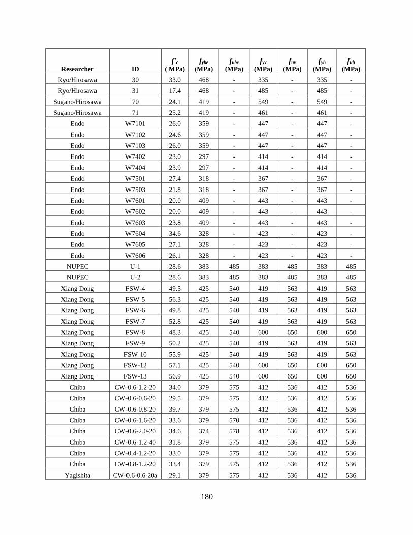
180

Researcher ID

f'c

( MPa)

fybe

(MPa)

fube

(MPa)

fyv

(MPa)

fuv

(MPa)

fyh

(MPa)

fuh

(MPa)

Ryo/Hirosawa 30 33.0 468 - 335 - 335 -

Ryo/Hirosawa 31 17.4 468 - 485 - 485 -

Sugano/Hirosawa 70 24.1 419 - 549 - 549 -

Sugano/Hirosawa 71 25.2 419 - 461 - 461 -

Endo W7101 26.0 359 - 447 - 447 -

Endo W7102 24.6 359 - 447 - 447 -

Endo W7103 26.0 359 - 447 - 447 -

Endo W7402 23.0 297 - 414 - 414 -

Endo W7404 23.9 297 - 414 - 414 -

Endo W7501 27.4 318 - 367 - 367 -

Endo W7503 21.8 318 - 367 - 367 -

Endo W7601 20.0 409 - 443 - 443 -

Endo W7602 20.0 409 - 443 - 443 -

Endo W7603 23.8 409 - 443 - 443 -

Endo W7604 34.6 328 - 423 - 423 -

Endo W7605 27.1 328 - 423 - 423 -

Endo W7606 26.1 328 - 423 - 423 -

NUPEC U-1 28.6 383 485 383 485 383 485

NUPEC U-2 28.6 383 485 383 485 383 485

Xiang Dong FSW-4 49.5 425 540 419 563 419 563

Xiang Dong FSW-5 56.3 425 540 419 563 419 563

Xiang Dong FSW-6 49.8 425 540 419 563 419 563

Xiang Dong FSW-7 52.8 425 540 419 563 419 563

Xiang Dong FSW-8 48.3 425 540 600 650 600 650

Xiang Dong FSW-9 50.2 425 540 419 563 419 563

Xiang Dong FSW-10 55.9 425 540 419 563 419 563

Xiang Dong FSW-12 57.1 425 540 600 650 600 650

Xiang Dong FSW-13 56.9 425 540 600 650 600 650

Chiba CW-0.6-1.2-20 34.0 379 575 412 536 412 536

Chiba CW-0.6-0.6-20 29.5 379 575 412 536 412 536

Chiba CW-0.6-0.8-20 39.7 379 575 412 536 412 536

Chiba CW-0.6-1.6-20 33.6 379 570 412 536 412 536

Chiba CW-0.6-2.0-20 34.6 374 578 412 536 412 536

Chiba CW-0.6-1.2-40 31.8 379 575 412 536 412 536

Chiba CW-0.4-1.2-20 33.0 379 575 412 536 412 536

Chiba CW-0.8-1.2-20 33.4 379 575 412 536 412 536

Yagishita CW-0.6-0.6-20a 29.1 379 575 412 536 412 536

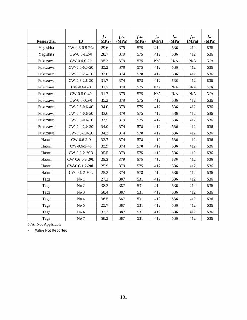
181

Researcher ID

f'c

( MPa)

fybe

(MPa)

fube

(MPa)

fyv

(MPa)

fuv

(MPa)

fyh

(MPa)

fuh

(MPa)

Yagishita CW-0.6-0.8-20a 29.6 379 575 412 536 412 536

Yagishita CW-0.6-1.2-0 28.7 379 575 412 536 412 536

Fukuzawa CW-0.6-0-20 35.2 379 575 N/A N/A N/A N/A

Fukuzawa CW-0.6-0.3-20 35.2 379 575 412 536 412 536

Fukuzawa CW-0.6-2.4-20 33.6 374 578 412 536 412 536

Fukuzawa CW-0.6-2.8-20 31.7 374 578 412 536 412 536



Fukuzawa CW-0.6-0.6-0 35.2 379 575 412 536 412 536

Fukuzawa CW-0.6-0.6-40 34.0 379 575 412 536 412 536

Fukuzawa CW-0.4-0.6-20 33.6 379 575 412 536 412 536

Fukuzawa CW-0.8-0.6-20 33.5 379 575 412 536 412 536

Fukuzawa CW-0.4-2.0-20 34.0 374 578 412 536 412 536

Fukuzawa CW-0.8-2.0-20 34.3 374 578 412 536 412 536

Hatori CW-0.6-2-0 33.7 374 578 412 536 412 536

Hatori CW-0.6-2-40 33.9 374 578 412 536 412 536

Hatori CW-0.6-2-20B 35.5 379 575 412 536 412 536

Hatori CW-0.6-0.6-20L 25.2 379 575 412 536 412 536

Hatori CW-0.6-1.2-20L 25.9 379 575 412 536 412 536

Hatori CW-0.6-2-20L 25.2 374 578 412 536 412 536

Taga No 1 27.2 387 531 412 536 412 536

Taga No 2 38.3 387 531 412 536 412 536

Taga No 3 58.4 387 531 412 536 412 536

Taga No 4 36.5 387 531 412 536 412 536

Taga No 5 25.7 387 531 412 536 412 536

Taga No 6 37.2 387 531 412 536 412 536

Taga No 7 58.2 387 531 412 536 412 536

N/A: Not Applicable

- Value Not Reported

182

Table A-8. Loading, strength and drift ratio of squat RC walls with enlarged boundary elements.

Researcher ID Loading

Type P/f'cAg

(%)

Vpeak (kN)

Rcr Rpeak Ru

Kabeyasawa/Hiraishi NW-2 Cyclic 10.2 1464 0.0026 0.0141 0.0169

Kabeyasawa/Hiraishi No. 1 Cyclic 13.1 1101 0.0019 0.0071 -

Kabeyasawa/Hiraishi No. 2 Cyclic 12.0 1208 0.0019 0.0071 0.0080





Kabeyasawa/Hiraishi No. 8 Cyclic 11.2 1638 0.0027 0.0074 0.0080

Sanada/Kabeyasawa Type N Cyclic 10.8 712 0.0011 0.0050 0.0095

Sanada/Kabeyasawa Type S Cyclic 9.8 702 0.0022 0.0063 -

Matsui Wall-A Dynamic 6.3 686 0.0016 0.0062 0.0115

Matsui Wall-B Dynamic 6.5 554 0.0017 0.0043 0.0124

Akita WAS Cyclic 6.6 654 0.0019 0.0076 0.0118

Akita WBS Cyclic 6.6 542 0.0019 0.0149 0.0175

Kabeyasawa K1 Cyclic 9.8 441 - - -




Maier S5 Cyclic 6.8 683 0.0029 0.0165 0.0177

Maier S7 Cyclic 27.9 855 0.0011 0.0063 0.0072

Barda B3-2 Cyclic 0.0 1039 0.0014 0.0052 0.0081

Barda B4-3 Cyclic 0.0 1017 0.0014 0.0053 0.0065

Barda B5-4 Cyclic 0.0 699 0.0003 0.0053 0.0134

Barda B6-4 Cyclic 0.0 876 0.0009 0.0061 0.0122

Barda B7-5 Cyclic 0.0 1075 0.0013 0.0126 0.0374

Barda B8-5 Cyclic 0.0 851 0.0009 0.0047 0.0096

Synge Wall-3 Cyclic 0.0 738 0.0010 0.0043 0.0065

Palermo/Vecchio DP1 Cyclic 5.4 1277 0.0012 0.0048 0.0058

Palermo/Vecchio DP2 Cyclic 0.0 892 0.0011 0.0039 0.0046

Saito W-15-1 Cyclic 7.9 2187 0.0015 0.0047 0.0075

Saito W-12-1 Cyclic 5.6 2658 0.0019 0.0055 0.0078

Saito W-12-2 Cyclic 5.1 2511 - - -

Saito W-12-3 Cyclic 5.5 2511 - - -

Saito W-12-4 Cyclic 2.7 2481 - - -

Saito W-12-5 Cyclic 4.9 2668 - - -

Saito W-15-2 Cyclic 7.6 1814 - - -

Saito W-12-6 Cyclic 5.9 1755 - - -

183


Type

P/f'cAg (%)

Vpeak (kN)

Rcr Rpeak Ru

Saito W-12-7 Cyclic 2.9 1648 - - -

Sato 18M 12-40 Cyclic 4.6 2250 - 0.0048 -

Sato 24M 8-30 Cyclic 5.3 1680 0.0006 0.0086 -

Sato 24M 8-40 Cyclic 5.6 1740 0.0007 0.0051 -

Sato 24M 8-50 Cyclic 5.7 1740 0.0007 0.0060 -

Sato 24M 6-30 Cyclic 5.0 2100 - 0.0088 -

Sato 24M 6-40 Cyclic 4.9 2190 - 0.0078 -

Sato 36M 12-30 Cyclic 5.5 2490 - 0.0062 -

Sato 36M 12-40 Cyclic 5.8 2490 - 0.0066 -

Sato 36M 12-50 Cyclic 5.4 2430 - 0.0060 -

Sato 36L 8-30 Cyclic 8.2 1800 - 0.0088 -

Sato 36L 8-40 Cyclic 7.2 1830 - 0.0083 -

Sato 36M 8-30 Cyclic 5.1 1890 0.0008 0.0088 -

Sato 36M 8-40 Cyclic 5.2 2040 0.0012 0.0070 0.0132

Sato 36M 8-50 Cyclic 5.3 1980 0.0015 0.0071 -

Sato 36M 6-30 Cyclic 6.0 2250 - 0.0082 -

Sato 36M 6-40 Cyclic 5.8 2370 - 0.0088 -

Sato 48M 8-30 Cyclic 7.3 1980 0.0014 0.0051 0.0084

Sato 48M 8-40 Cyclic 7.3 2040 0.0017 0.0063 -

Sato 48M 8-50 Cyclic 7.1 2040 0.0019 0.0063 -

Sato 48H 8-30 Cyclic 4.8 2280 - 0.0053 -

Sato 48H 8-40 Cyclic 4.6 2340 - 0.0053 -

Sato 48H 8-50 Cyclic 4.5 2430 - 0.0083 -

Seki RA-00P Pseudo Dyn. 0.0 1473 - - -

Seki RA-15P Pseudo Dyn. 3.4 1671 0.0009 0.0060 0.0097

Seki RB-00P Pseudo Dyn. 0.0 1264 - - -

Seki RB-15P Pseudo Dyn. 3.5 1464 0.0009 0.0053 0.0060

Seki RC-00P Pseudo Dyn. 0.0 1032 - - -

Seki RC-15P Pseudo Dyn. 3.5 1170 0.0009 0.0045 0.0096

Park S4 Cyclic 7.3 2544.5 0.0039 0.0100 0.0136

Dabbagh SW1 Cyclic 10.3 999.5 0.0041 0.0109 -

Dabbagh SW2 Cyclic 10.3 1191 0.0059 0.0137 0.0145

Dabbagh SW3 Cyclic 9.3 1098.5 0.0041 0.0111 0.0121

Dabbagh SW4 Cyclic 0.0 718 0.0039 0.0092 0.0117

Dabbagh SW5 Cyclic 10.7 1103.5 0.0042 0.0109 0.0118

Dabbagh SW6 Cyclic 10.7 1121 0.0056 0.0140 -

Ryo/Hirosawa 30 Cyclic 0.0 829 0.0009 0.0030 -

Ryo/Hirosawa 31 Cyclic 0.0 534 0.0010 0.0038 -

Sugano/Hirosawa 70 Cyclic 0.0 707 0.0010 0.0030 0.0044

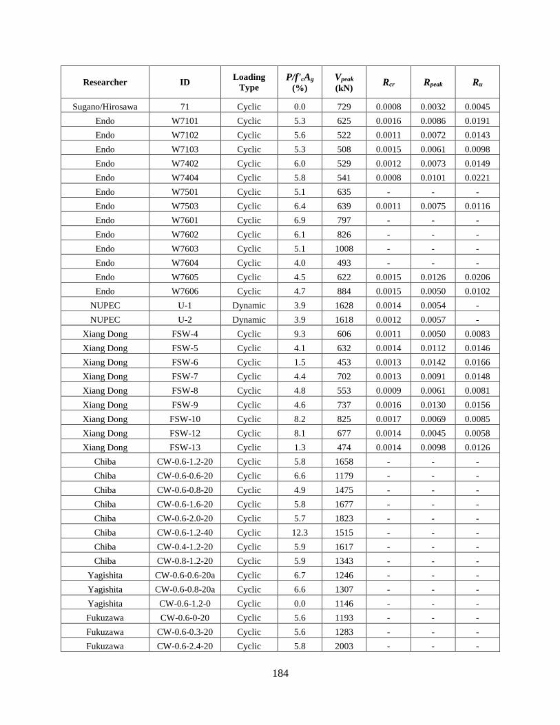
184


Type

P/f'cAg (%)

Vpeak (kN)

Rcr Rpeak Ru

Sugano/Hirosawa 71 Cyclic 0.0 729 0.0008 0.0032 0.0045

Endo W7101 Cyclic 5.3 625 0.0016 0.0086 0.0191

Endo W7102 Cyclic 5.6 522 0.0011 0.0072 0.0143

Endo W7103 Cyclic 5.3 508 0.0015 0.0061 0.0098

Endo W7402 Cyclic 6.0 529 0.0012 0.0073 0.0149

Endo W7404 Cyclic 5.8 541 0.0008 0.0101 0.0221

Endo W7501 Cyclic 5.1 635 - - -

Endo W7503 Cyclic 6.4 639 0.0011 0.0075 0.0116

Endo W7601 Cyclic 6.9 797 - - -

Endo W7602 Cyclic 6.1 826 - - -

Endo W7603 Cyclic 5.1 1008 - - -

Endo W7604 Cyclic 4.0 493 - - -

Endo W7605 Cyclic 4.5 622 0.0015 0.0126 0.0206

Endo W7606 Cyclic 4.7 884 0.0015 0.0050 0.0102

NUPEC U-1 Dynamic 3.9 1628 0.0014 0.0054 -

NUPEC U-2 Dynamic 3.9 1618 0.0012 0.0057 -

Xiang Dong FSW-4 Cyclic 9.3 606 0.0011 0.0050 0.0083









Chiba CW-0.6-1.2-20 Cyclic 5.8 1658 - - -

Chiba CW-0.6-0.6-20 Cyclic 6.6 1179 - - -

Chiba CW-0.6-0.8-20 Cyclic 4.9 1475 - - -

Chiba CW-0.6-1.6-20 Cyclic 5.8 1677 - - -

Chiba CW-0.6-2.0-20 Cyclic 5.7 1823 - - -

Chiba CW-0.6-1.2-40 Cyclic 12.3 1515 - - -

Chiba CW-0.4-1.2-20 Cyclic 5.9 1617 - - -

Chiba CW-0.8-1.2-20 Cyclic 5.9 1343 - - -

Yagishita CW-0.6-0.6-20a Cyclic 6.7 1246 - - -

Yagishita CW-0.6-0.8-20a Cyclic 6.6 1307 - - -

Yagishita CW-0.6-1.2-0 Cyclic 0.0 1146 - - -

Fukuzawa CW-0.6-0-20 Cyclic 5.6 1193 - - -

Fukuzawa CW-0.6-0.3-20 Cyclic 5.6 1283 - - -


185


Type

P/f'cAg (%)

Vpeak (kN)

Rcr Rpeak Ru










Hatori CW-0.6-2-0 Cyclic 0.0 1712 - - -

Hatori CW-0.6-2-40 Cyclic 11.6 2035 - - -

Hatori CW-0.6-2-20B Cyclic 5.5 1775 - - -

Hatori CW-0.6-0.6-20L Cyclic 7.8 1276 - - -

Hatori CW-0.6-1.2-20L Cyclic 7.6 1390 - - -

Hatori CW-0.6-2-20L Cyclic 7.8 1491 - - -

Taga No 1 Cyclic 7.2 1088 - - -

Taga No 2 Cyclic 5.1 1334 - - -

Taga No 3 Cyclic 3.4 1461 - - -

Taga No 4 Cyclic 5.4 1236 - - -

Taga No 5 Cyclic 7.6 1137 - - -

Taga No 6 Cyclic 5.3 1461 - - -

Taga No 7 Cyclic 3.4 1677 - - -

- Corresponding drift ratio value could not be obtained from the reported data.

186

APPENDIX B OPENSEES HYSTERETIC MODEL

INPUT FILE EXAMPLE

# ================================================================

# Squat RC Shear Walls Hysteretic Behavior Modeling

# Carlos M. Adorno ([email protected])

# University of Puerto Rico at Mayaguez

# ===================== DESCRIPTION ==============================

# Date: NOV 3, 2013 #

# Wall's behavior modeled as a single truss element with unit length and unit area

#_____________ <----> Q

# L=1,A=1 _O_

# Hysteretic behavior at the uniaxial material: Hysteretic Material

# Refer to Hysteretic Material at oppensees wiki for full explanation of the material model &

parameters

# Model subjected to reverse Cyclic Loading - using procedure: procRCycDAns.tcl (By: N.

Mitra)

# File Name: RCyclicHyst.tcl

# Experimental Test: SW1 (NEES/Buffalo)

# Units: lb, in (Other units can be used)

# ======================= DATA DIRECTORY =========================

wipe; # removes all constructed objects

set dataDir DataOut_SW1; # set up name of output data directory

file mkdir $dataDir; # create data directory

#=========================== BACKBONE ===========================

# Positive envelope Load vs Drift

set Qcr 181.1; # Cracking Shear

set Drifcr 0.00193; # Cracking Drift

set Qy 256; # Yielding Shear

set Drify 0.0134; # Yielding Drift

set Qcap 171.28; # Capping Shear

set Drifcap 0.0252; # Capping Drift

# Negative envelope Load vs Drift

set Qcrn -179; # Cracking Shear - neg. branch

set Drifcrn -0.000926; # Cracking Drift - neg. branch

set Qyn -250; # Yielding Shear - neg. branch

set Drifyn -0.0128; # Yielding Drift - neg. branch

set Qcapn -242; # Capping Shear - neg. branch

187

set Drifcapn -0.0173; # Capping Drift - neg. branch

# Hysteretic Behavior Parameters

set pinchX 0.6; # pinching factor for strain (or deformation) during reloading

set pinchY 0.15; # pinching factor for stress (or force) during reloading

set damage1 0.01; # damage due to ductility: D1(mu-1)

set damage2 0; # damage due to energy: D2(Eii/Eult)

set beta 0.3; # power used to determine the degraded unloading stiffness based on

ductility

puts "OK hyst param read"

# =============== END OF INPUT DATA (Exept displacement peaks)=============

# -------------------------------- MODEL SET UP ---------------------------------

model BasicBuilder -ndm 2 -ndf 2; # define spatial dimension of model and number of DOF per

node

# add nodes - command: node nodeId xCrd yCrd

node 1 0.0 0.0; # start node

node 2 1.0 0.0; # end node

#*** keep the follwoing procedure on the same directory of the model ***#

#source procRCycDAns.tcl; # procedure to apply the reversed cyclic pushover

#------------------------ UNIAXIAL MATERIAL GENERATION --------------------------

set matID 1; # material ID: assigns a tag number to the material behavior

# add the material to domain

uniaxialMaterial Hysteretic $matID $Qcr $Drifcr $Qy $Drify $Qcap $Drifcap $Qcrn $Drifcrn

$Qyn $Drifyn $Qcapn $Drifcapn $pinchX $pinchY $damage1 $damage2 $beta;

puts "OK material created"

#-------------------------- TRUSS ELEMENT GENERATION ----------------------------

# Element Conectivity

# add truss elements - command: element truss trussID node1 node2 A matID

element truss 1 1 2 1.0 1;

#------------------------------ Boundary Conditions -----------------------------

fix 1 1 1; # command: fix nodeID xResrnt? yRestrnt? (1=fixed; 0=free)

fix 2 0 1;

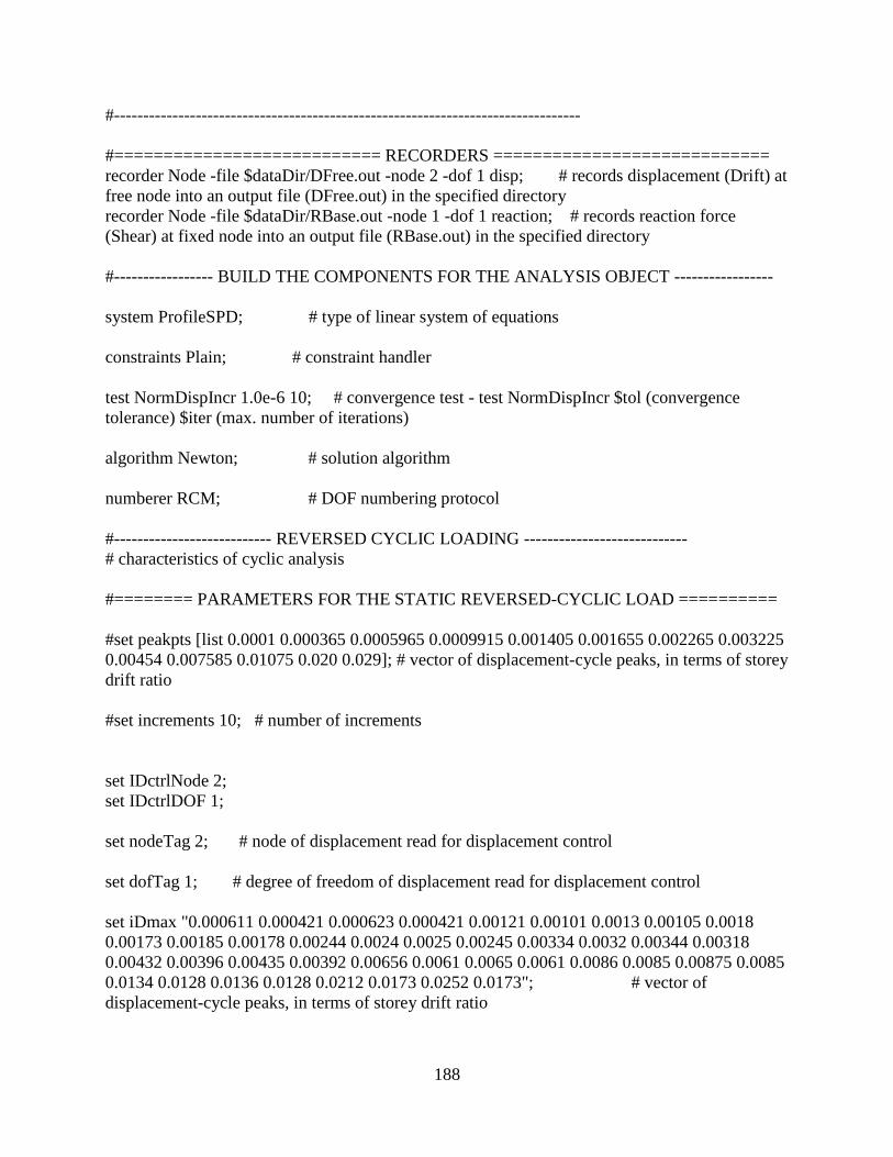
188

#--------------------------------------------------------------------------------

#=========================== RECORDERS ============================

recorder Node -file $dataDir/DFree.out -node 2 -dof 1 disp; # records displacement (Drift) at

free node into an output file (DFree.out) in the specified directory

recorder Node -file $dataDir/RBase.out -node 1 -dof 1 reaction; # records reaction force

(Shear) at fixed node into an output file (RBase.out) in the specified directory

#----------------- BUILD THE COMPONENTS FOR THE ANALYSIS OBJECT -----------------

system ProfileSPD; # type of linear system of equations

constraints Plain; # constraint handler

test NormDispIncr 1.0e-6 10; # convergence test - test NormDispIncr $tol (convergence

tolerance) $iter (max. number of iterations)

algorithm Newton; # solution algorithm

numberer RCM; # DOF numbering protocol

#--------------------------- REVERSED CYCLIC LOADING ----------------------------

# characteristics of cyclic analysis

#======== PARAMETERS FOR THE STATIC REVERSED-CYCLIC LOAD ==========

#set peakpts [list 0.0001 0.000365 0.0005965 0.0009915 0.001405 0.001655 0.002265 0.003225

0.00454 0.007585 0.01075 0.020 0.029]; # vector of displacement-cycle peaks, in terms of storey

drift ratio

#set increments 10; # number of increments

set IDctrlNode 2;

set IDctrlDOF 1;

set nodeTag 2; # node of displacement read for displacement control

set dofTag 1; # degree of freedom of displacement read for displacement control

set iDmax "0.000611 0.000421 0.000623 0.000421 0.00121 0.00101 0.0013 0.00105 0.0018

0.00173 0.00185 0.00178 0.00244 0.0024 0.0025 0.00245 0.00334 0.0032 0.00344 0.00318

0.00432 0.00396 0.00435 0.00392 0.00656 0.0061 0.0065 0.0061 0.0086 0.0085 0.00875 0.0085

0.0134 0.0128 0.0136 0.0128 0.0212 0.0173 0.0252 0.0173"; # vector of

displacement-cycle peaks, in terms of storey drift ratio

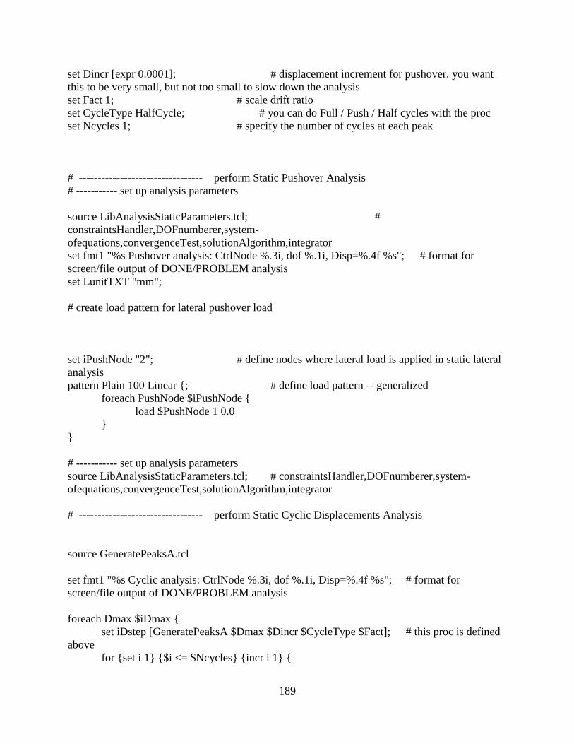
189

set Dincr [expr 0.0001]; # displacement increment for pushover. you want

this to be very small, but not too small to slow down the analysis

set Fact 1; # scale drift ratio

set CycleType HalfCycle; # you can do Full / Push / Half cycles with the proc

set Ncycles 1; # specify the number of cycles at each peak

# --------------------------------- perform Static Pushover Analysis

# ----------- set up analysis parameters

source LibAnalysisStaticParameters.tcl; #

constraintsHandler,DOFnumberer,system-

ofequations,convergenceTest,solutionAlgorithm,integrator

set fmt1 "%s Pushover analysis: CtrlNode %.3i, dof %.1i, Disp=%.4f %s"; # format for

screen/file output of DONE/PROBLEM analysis

set LunitTXT "mm";

# create load pattern for lateral pushover load

set iPushNode "2"; # define nodes where lateral load is applied in static lateral

analysis

pattern Plain 100 Linear {; # define load pattern -- generalized

foreach PushNode $iPushNode {

load $PushNode 1 0.0

}

}

# ----------- set up analysis parameters

source LibAnalysisStaticParameters.tcl; # constraintsHandler,DOFnumberer,system-

ofequations,convergenceTest,solutionAlgorithm,integrator

# --------------------------------- perform Static Cyclic Displacements Analysis

source GeneratePeaksA.tcl

set fmt1 "%s Cyclic analysis: CtrlNode %.3i, dof %.1i, Disp=%.4f %s"; # format for

screen/file output of DONE/PROBLEM analysis

foreach Dmax $iDmax {

set iDstep [GeneratePeaksA $Dmax $Dincr $CycleType $Fact]; # this proc is defined

above

for {set i 1} {$i <= $Ncycles} {incr i 1} {

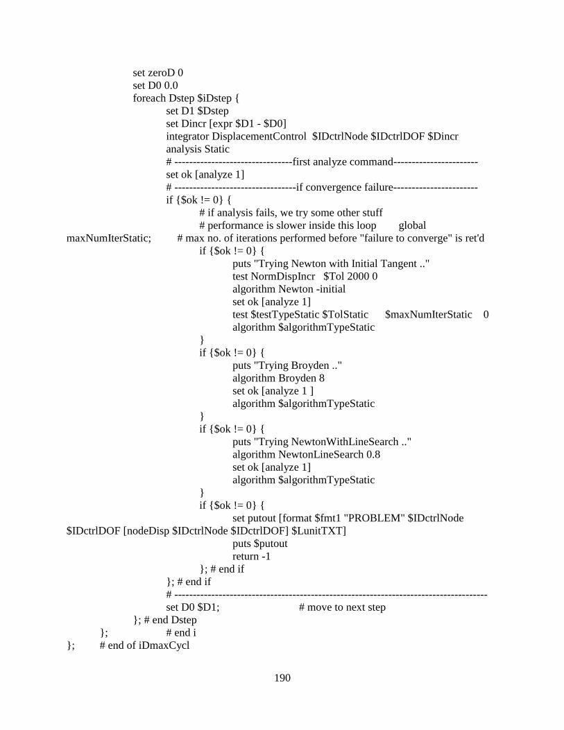
190

set zeroD 0

set D0 0.0

foreach Dstep $iDstep {

set D1 $Dstep

set Dincr [expr $D1 - $D0]

integrator DisplacementControl $IDctrlNode $IDctrlDOF $Dincr

analysis Static

# --------------------------------first analyze command-----------------------

set ok [analyze 1]

# ---------------------------------if convergence failure-----------------------

if {$ok != 0} {

# if analysis fails, we try some other stuff

# performance is slower inside this loop global

maxNumIterStatic; # max no. of iterations performed before "failure to converge" is ret'd

if {$ok != 0} {

puts "Trying Newton with Initial Tangent .."

test NormDispIncr $Tol 2000 0

algorithm Newton -initial

set ok [analyze 1]

test $testTypeStatic $TolStatic $maxNumIterStatic 0

algorithm $algorithmTypeStatic

}

if {$ok != 0} {

puts "Trying Broyden .."

algorithm Broyden 8

set ok [analyze 1 ]


}

if {$ok != 0} {

puts "Trying NewtonWithLineSearch .."

algorithm NewtonLineSearch 0.8

set ok [analyze 1]


}

if {$ok != 0} {

set putout [format $fmt1 "PROBLEM" $IDctrlNode

$IDctrlDOF [nodeDisp $IDctrlNode $IDctrlDOF] $LunitTXT]

puts $putout

return -1

}; # end if

}; # end if

# -------------------------------------------------------------------------------------

set D0 $D1; # move to next step

}; # end Dstep

}; # end i

}; # end of iDmaxCycl

191

# -----------------------------------------------------------------------------------------------------

if {$ok != 0 } {

puts [format $fmt1 "PROBLEM" $IDctrlNode $IDctrlDOF [nodeDisp $IDctrlNode

$IDctrlDOF] $LunitTXT]

} else {

puts [format $fmt1 "DONE" $IDctrlNode $IDctrlDOF [nodeDisp $IDctrlNode

$IDctrlDOF] $LunitTXT]

}

print node; # print the results at nodes

print node; # print the results at nodes

192

APPENDIX C OPENSEES FLEXURE-SHEAR

INTERACTION MODEL INPUT FILE

EXAMPLE

# file to analyze a RC wall using the flexure-shear interaction element

# this file is intended to model an individual wall with rectangular cross section and uniformly

distributed vertical and horizontal reinforcement

wipe; # clear memory of all past model definitions

model BasicBuilder -ndm 2 -ndf 3; # Define the model builder, ndm=#dimension, ndf=#dofs

set dataDir wall_SW1; # set up name of data directory (can remove this)

file mkdir $dataDir; # create data directory

#set GMdir "../GMfiles/";

# units psi, in (this can be changed while maintaining consistent units)

# Analysis parameters---------------------------------------------------------------------

set tolAx 1.0e-5; set iterAx 100;

set tolLatNew .00035; set iterLatNew 8000;

set tolLatIni 1.0e-3; set iterLatIni 1000;

set dUi 0.001; # Displacement increment

set maxU 2.3; # Max. Displacement

#Nodes--------------------------------------------------------------------------------------------------------

#Define nodal coordinates

#set n 7

set y1 0; set y2 16.11; set y3 32.22; set y4 48.33; set y5 64.44;

set y6 80.55; set y7 96.66; set y8 112.8;

#Define nodes by assigning defined coordinates

node 1 0 $y1 0; node 3 0 $y2 0; node 4 0 $y3 0; node 5 0 $y4 0;

node 6 0 $y5 0; node 7 0 $y6 0; node 8 0 $y7 0; node 2 0 $y8 0;

#Define fixed base boundary condition

fix 1 1 1 1;

print node;

# Set up parameters that are particular to the model for displacement control

set IDctrlNode 2; # node where displacement is read for displacement control

193

set IDctrlDOF 1; # degree of freedom of displacement read for displacement control

#concrete parameters for Concrete 06 uniaxial model----------------------------------------------------

# Unconfined concrete

set fc -3600; set eo -0.003; set nc 2; set k 1; set fcr 450; set alphaC 0.32; set ecr 0.00008; set b 4;

set alphaT 0.08;

#steel parameters for Steel 02 uniaxial model----------------------------------------------------------

#steel02($Fy $E $b $R0 $CR1 $CR2 $a1 $a2 $a3 $a4)

# Vertical steel web

set fyv 67300; set E 29000000; set bs 0.018; set Ro 15; set cR1 0.925; set cR2 0.15; set a1 18.5;

set a2 0.0015; set a3 0; set a4 1.0;

# Vertical steel boundary element

#set fyvb 413.9; set Eb 200000; set bsb 0.016; set Rob 15; set cR1b 0.925; set cR2b 0.15; set a1b

18.5; set a2b 0.0015;

# Horizontal steel

set fyh 67300; set Eh 29000000; set bsh 0.018; set Roh 15; set cR1h 0.925; set cR2h 0.15; set

a1h 18.5; set a2h 0.0015; set a3h 0; set a4h 1.0;

#concrete (confined and unconfined)-----------------------------------------------------------------------

#uniaxialMaterial Concrete06 $matTag $fc $e0 $n $k $alpha1 $fcr $ecr $b $alpha2

#uniaxialMaterial Concrete06 1 $fcc $ecc $ncc $kcc $alphaC $fcrc $ecr $b $alphaT;

uniaxialMaterial Concrete06 2 $fc $eo $nc $k $alphaC $fcr $ecr $b $alphaT;

#Steel (vertical and horizontal)-----------------------------------------------------------------------------

#web steel

uniaxialMaterial Steel02 1002 $fyv $E $bs $Ro $cR1 $cR2 $a1 $a2 $a3 $a4;

#boundary element steel

#uniaxialMaterial Steel02 1003 $fyvb $Eb $bsb $Rob $cR1b $cR2b $a1b $a2b;

#horiz. steel

uniaxialMaterial Steel02 1004 $fyh $Eh $bsh $Roh $cR1h $cR2h $a1h $a2h $a3h $a4h;

194

# Define cross-section-----------------------------------------------------------------------------------------

set t1 8; set NStrip1 1; # thickness 1



geomTransf LinearInt 1

set np 1; # int. points

set C 0.4; # center of rotation

# Section definition ------------------------------------------------------------------------------------------

#section FiberInt $secTag -NStrip $nStrip1 $thick1 $nStrip2 $thick2 $nStrip3 $thick3

{fiber...Hfiber ...}

#fiber $yLoc $zLoc $A $matTag

#coordinates for each strip

set yLoc 3.43; set yLoc1 10.28; set yLoc2 17.13; set yLoc3 23.98; set yLoc4 30.84;

set yLoc5 37.69; set yLoc6 44.54; set yLoc7 51.40; set yLoc8 55.66; set yLoc9 58.25

set zLoc 0;

# Tributary areas for each strip

set Au1 54.42; set Au2 13.41; set Au3 27.6

set As1 0.4

set Ah 0.8;

#---------

section FiberInt 2 -NStrip $NStrip1 $t1 $NStrip2 $t2 $NStrip3 $t3 {

#vertical fibers

fiber -$yLoc9 $zLoc $Au3 2; fiber -$yLoc9 $zLoc $As1 1002;

fiber -$yLoc8 $zLoc $Au2 2;



195






fiber -$yLoc $zLoc $Au1 2; fiber -$yLoc $zLoc $As1 1002;

fiber $yLoc $zLoc $Au1 2; fiber $yLoc $zLoc $As1 1002;

fiber $yLoc1 $zLoc $Au1 2; fiber $yLoc1 $zLoc $As1 1002;







fiber $yLoc8 $zLoc $Au2 2;


#horiz. reinf.

Hfiber 0 $zLoc $Ah 1004;

}

# Element definition-------------------------------------------------------------------------------------------

#element dispBeamColumnInt $eleTag $iNode $jNode $numIntgrPts $secTag $transfTag $cRot

element dispBeamColumnInt 1 1 3 $np 2 1 $C


196






print element;

# Create a recorder to monitor nodal displacement and element forces---------------------------------

recorder Node -file $dataDir/nodeTop.out -time -node 2 -dof 1 2 3 disp;

recorder Element -file $dataDir/elesX.out -time -ele 1 globalForce;

# recorder for element1 section1 steel stress/strain and section force-def.-----------------------------

recorder Element -file $dataDir/Sect_FandD.out -ele 1 section 1 forceAndDeformation

recorder Element -file $dataDir/Sect_FandD2.out -ele 1 section 2 forceAndDeformation

recorder Element -file $dataDir/Sect_eX.out -ele 1 section 1 eX

recorder Element -file $dataDir/Sect_eY.out -ele 1 section 1 eY

recorder Element -file $dataDir/Sect_sXsteel.out -ele 1 section 1 sX

recorder Element -file $dataDir/Sect_sYsteel.out -ele 1 section 1 sY

recorder Element -file $dataDir/Sect_e1.out -ele 1 section 1 e1

recorder Element -file $dataDir/Sect_e2.out -ele 1 section 1 e2

recorder Element -file $dataDir/Sect_s1conc.out -ele 1 section 1 s1

recorder Element -file $dataDir/Sect_s2conc.out -ele 1 section 1 s2

recorder Element -file Element1.out -time -ele 1 section 1 fiber 0 0 stressStrain

197

# Set axial load-------------------------------------------------------------------------------------------------

set PCol 0;

pattern Plain 1 Constant {

load 2 0 -$PCol 0;

}

# Gravity-analysis parameters -- load-controlled static analysis

initialize; integrator LoadControl 0;

system SparseGeneral -piv; test NormUnbalance $tolAx $iterAx 0;

numberer Plain; constraints Plain;

algorithm ModifiedNewton -initial; analysis Static;

# perform the gravity load analysis,

analyze [expr 1]

loadConst -time 0.0

# ------------------------------------ maintain constant gravity loads and reset time to zero

puts "Model Built"

# create load pattern for lateral pushover load

pattern Plain 200 Linear {; # define load pattern -- generalized

load 2 100 0.0 0.0 ; # define lateral load in static lateral analysis

}

test NormDispIncr $tolLatNew $iterLatNew;

algorithm Newton -initial

analysis Static

198

set dU $dUi;

set numSteps [expr int($maxU/$dU)];

integrator DisplacementControl 2 1 $dU 1 $dU $dU

#source cycle2.tcl

#### end

set ok [analyze $numSteps]; set jump 1;

if {$ok != 0} {

set currentDisp [nodeDisp 2 1]

set ok 0

while {abs($currentDisp) < abs($maxU)} {

set ok [analyze 1]

puts "\n Trying.. $currentDisp\n"

# if the analysis fails try initial tangent iteration

if {$ok != 0} {

puts "\n regular newton failed .. try an initial stiffness"

test NormDispIncr $tolLatIni $iterLatIni 0;

algorithm ModifiedNewton -initial ;

set ok [analyze 1]

puts "\n Trying.. $currentDisp\n"

if {$ok == 0} {

puts " that worked .. back to regular newton \n"

set jump 1

199

integrator DisplacementControl 2 1 $dU 1

} else {

puts "\n that didn't worked .. Try next point\n"

set jump [expr $jump+1];

integrator DisplacementControl 2 1 [expr $dU*$jump] 1

}

test NormDispIncr $tolLatNew $iterLatNew

algorithm Newton

} else {set jump 1

integrator DisplacementControl 2 1 $dU 1

}

set currentDisp [expr $currentDisp+$dU]

}

}

#### end

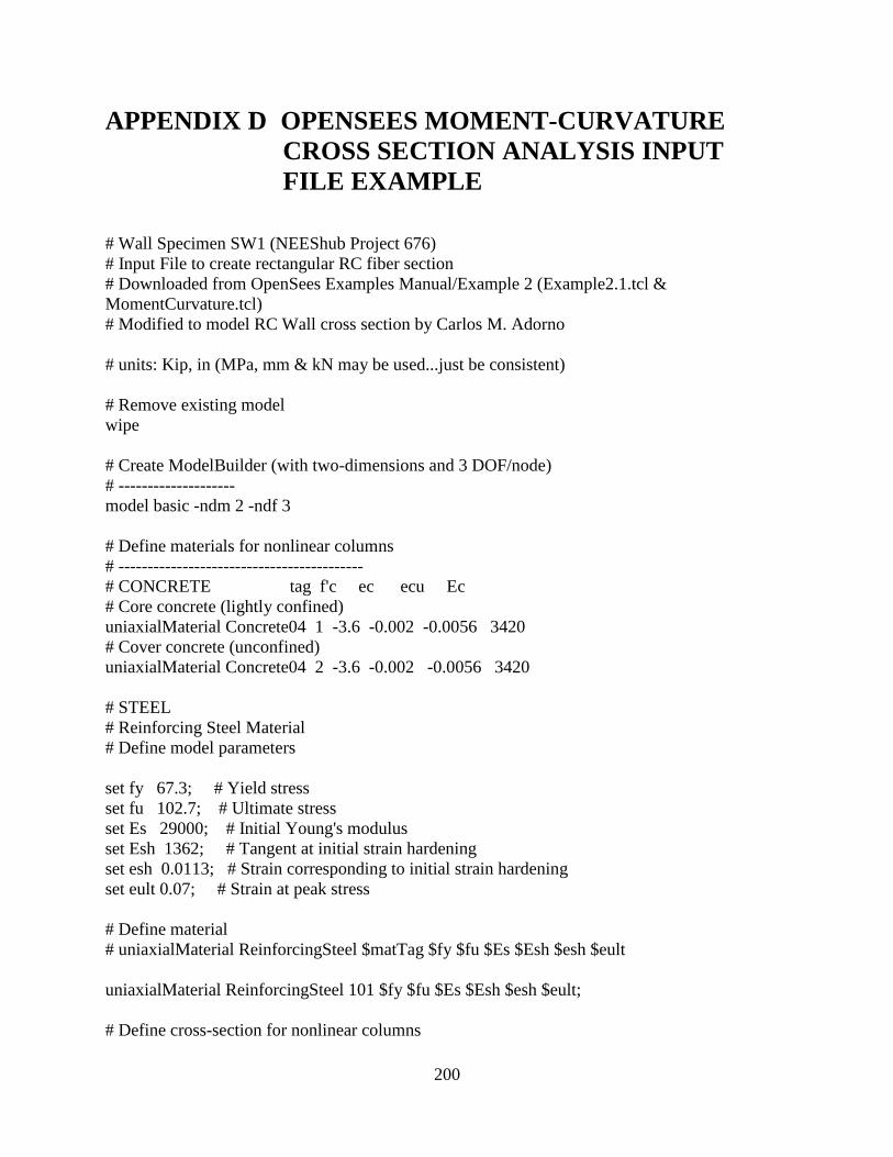
200

APPENDIX D OPENSEES MOMENT-CURVATURE

CROSS SECTION ANALYSIS INPUT

FILE EXAMPLE

# Wall Specimen SW1 (NEEShub Project 676)

# Input File to create rectangular RC fiber section

# Downloaded from OpenSees Examples Manual/Example 2 (Example2.1.tcl &

MomentCurvature.tcl)

# Modified to model RC Wall cross section by Carlos M. Adorno

# units: Kip, in (MPa, mm & kN may be used...just be consistent)

# Remove existing model

wipe

# Create ModelBuilder (with two-dimensions and 3 DOF/node)

# --------------------

model basic -ndm 2 -ndf 3

# Define materials for nonlinear columns

# ------------------------------------------

# CONCRETE tag f'c ec ecu Ec

# Core concrete (lightly confined)

uniaxialMaterial Concrete04 1 -3.6 -0.002 -0.0056 3420

# Cover concrete (unconfined)

uniaxialMaterial Concrete04 2 -3.6 -0.002 -0.0056 3420

# STEEL

# Reinforcing Steel Material

# Define model parameters

set fy 67.3; # Yield stress

set fu 102.7; # Ultimate stress

set Es 29000; # Initial Young's modulus

set Esh 1362; # Tangent at initial strain hardening

set esh 0.0113; # Strain corresponding to initial strain hardening

set eult 0.07; # Strain at peak stress

# Define material

# uniaxialMaterial ReinforcingSteel $matTag $fy $fu $Es $Esh $esh $eult

uniaxialMaterial ReinforcingSteel 101 $fy $fu $Es $Esh $esh $eult;

# Define cross-section for nonlinear columns

201

# ------------------------------------------

# set some paramaters

set tw 8; # wall thickness

set lw 120; # wall length

set cover 1.5; # concrete clear cover

set As 0.20; # area of no. 4 bars

# some variables derived from the parameters

set y1 [expr $lw/2.0]

set z1 [expr $tw/2.0]

section Fiber 1 {

# Create the concrete core fibers

# patch rect $matTag $numSubdivY $numSubdivZ $yI $zI $yJ $zJ

patch rect 1 120 1 [expr $cover-$y1] [expr $cover-$z1] [expr $y1-$cover] [expr $z1-$cover]

# Create the concrete cover fibers (bottom,top,right, left)

patch rect 2 120 1 [expr $cover-$y1] [expr $z1-$cover] [expr $y1-$cover] $z1

patch rect 2 120 1 [expr $cover-$y1] [expr -$z1] [expr $y1-$cover] [expr $cover-$z1]

patch rect 2 2 1 [expr -$y1] [expr -$z1] [expr $cover-$y1] $z1

patch rect 2 2 1 [expr $y1-$cover] [expr -$z1] $y1 $z1

# Create the reinforcing fibers (bottom, top)

# layer straight $matTag $numFiber $areaFiber $yStart $zStart $yEnd $zEnd

layer straight 101 17 $As [expr $cover-$y1] [expr $cover-$z1] [expr $y1-$cover] [expr

$cover-$z1]

layer straight 101 17 $As [expr $cover-$y1] [expr $z1-$cover] [expr $y1-$cover] [expr $z1-

$cover]

}

# Estimate yield curvature

# (Assuming no axial load and only top and bottom steel)

set d [expr $lw-$cover] ;# d -- from cover to rebar

set epsy [expr $fy/$Es] ;# steel yield strain

# Yield furvature for walls (Paulay & Priestley Seismic Design of RC & Masonry Buildings pp.

405)

set Ky [expr 0.0033/$lw]

#set Ky [expr $epsy/(0.7*$d)] # For other sections (OpenSees Example)

# Print estimate to standard output

puts "Estimated yield curvature: $Ky"

# Set axial load

set P 0

202

set mu 100; # Target ductility for analysis

set numIncr 1000; # Number of analysis increments

# Call the section analysis procedure

source MomentCurvature.tcl

MomentCurvature 1 $P [expr $Ky*$mu] $numIncr

shear strength and displacement …prltap.org/eng/wp-content/uploads/2017/10/carlos-adorno.pdfshear...

Documents