ascalablearchitecturefortheinterconnectionof microgrids
TRANSCRIPT

A Scalable Architecture for the Interconnection ofMicrogrids
byAllison FeroB.A. Physics
University of California (2013)Submitted to the Institute for Data, Systems, and Societyin partial fulfillment of the requirements for the degree of
Master of Science in Technology and Policyat the
MASSACHUSETTS INSTITUTE OF TECHNOLOGYJune 2017
c○ Massachusetts Institute of Technology 2017. All rights reserved.
Author . . . . . . . . . . . . . . . . . . . . . . . . . . . . . . . . . . . . . . . . . . . . . . . . . . . . . . . . . . . . . . . .Institute for Data, Systems, and Society
May 12, 2017Certified by. . . . . . . . . . . . . . . . . . . . . . . . . . . . . . . . . . . . . . . . . . . . . . . . . . . . . . . . . . . .
Munther DahlehWilliam A. Coolidge Professor, Electrical Engineering and Computer
ScienceThesis Supervisor
Certified by. . . . . . . . . . . . . . . . . . . . . . . . . . . . . . . . . . . . . . . . . . . . . . . . . . . . . . . . . . . .Mardavij Roozbehani
Senior Research ScientistLaboratory for Information and Decision Systems
Thesis SupervisorAccepted by . . . . . . . . . . . . . . . . . . . . . . . . . . . . . . . . . . . . . . . . . . . . . . . . . . . . . . . . . . .
Munther DahlehWilliam A. Coolidge Professor, Electrical Engineering and Computer
ScienceDirector of the Institute for Data, Systems, and Society

2
A Scalable Architecture for the Interconnection of Microgrids
by
Allison Fero
Submitted to the Institute for Data, Systems, and Societyon May 12, 2017, in partial fulfillment of the
requirements for the degree ofMaster of Science in Technology and Policy
Abstract
Electrification is a global challenge that is especially acute in India, where about onefifth of the population has no access to electricity. Solar powered microgrid technologyis a viable central grid alternative in the electrification of India, especially in remoteareas where grid extension is cost prohibitive. However, the upfront costs of microgriddevelopment, coupled with inadequate financing, have led to the implementation ofsmall scale, stand alone systems. Thus, the costs of local generation and storage area substantial barrier to acquisition of the technology. Furthermore, the issues of un-certainty, intermittency, and variability of renewable generation are daunting in smallmicrogrids due to lack of aggregation. In this work, a methodology is provided thatmaximizes system-wide reliability through the design of a computationally scalablecommunication and control architecture for the interconnection of microgrids. Anoptimization based control system is proposed that finds optimal load scheduling andenergy sharing decisions subject to system dynamics, power balance constraints, andcongestion constraints, while maximizing network-wide reliability. The model is firstformulated as a centralized optimization problem, and the value of interconnectionis assessed using supply and demand data gathered in India. The model is then for-mulated as a layered decomposition, in which local scheduling optimization occurs ateach microgrid, requiring only nearest neighbor communication to ensure feasibilityof the solutions. Finally, a methodology is proposed to generate distributed optimalpolicies for a network of Linear Quadratic Regulators that are each making decisionscoupled by network flow constraints. The LQR solution is combined with networkflow dual decomposition to generate a fully decomposed algorithm for finding thedynamic programming solution of the LQR subject to network flow constraints.
Thesis Supervisor: Munther DahlehTitle: William A. Coolidge Professor, Electrical Engineering and Computer Science
Thesis Supervisor: Mardavij RoozbehaniTitle: Senior Research ScientistLaboratory for Information and Decision Systems
3

4

Acknowledgments
I am incredibly thankful for the experience I have had at MIT over the last two
years, and the amount of support that I received on the way. First I must thank my
advisors Professor Munther Dahleh and Dr. Mardavij Roozbehani. The growth that
I experienced while I was at MIT would not have been possible without them, and
their depth of knowledge never fails to surprise me. It was a priviledge to develop my
research with such talented advisors. I’d like to thank the other members of LIDS
for such a warm and stimulating community, especially Dr. Daria Madjidian, whose
patience allowed for many multi-houred discussions. I’d also like to thank the Tata
Center for Technology and Design, as well as Professor Rajeev Ram and Dr. Reja
Amataya, for providing the resources that allowed me to explore otherwise theoretical
ideas in such an important and applied domain as electrification in India.
Finally, I must thank my friends and family for being my foundation throughout
this experience. The Technology and Policy Program attracts an incredible cohort of
people who have been indispensable to my success at MIT. Thank you to my friends
all over the world who never missed a beat, and even visited me across the country.
Thank you to my sisters Kelly and Shelby and my brother Mostyn for the consistent
group text updates, check-ins, and phone calls. Thank you Kyle for being there when
I needed support of any kind, and being selfless without hesitation over the last couple
years. And thank you to my parents, Mike and Katy, for all of the encouragement
that got me to MIT and the unconditional love and guidance that inspire me every
day.
5

6

Contents
1 Electrification in India 9
1.1 Motivation . . . . . . . . . . . . . . . . . . . . . . . . . . . . . . . . . 9
1.2 Political Landscape . . . . . . . . . . . . . . . . . . . . . . . . . . . . 10
1.2.1 Energy Policies . . . . . . . . . . . . . . . . . . . . . . . . . . 10
1.2.2 Implementation . . . . . . . . . . . . . . . . . . . . . . . . . . 11
1.3 Microgrids in India . . . . . . . . . . . . . . . . . . . . . . . . . . . . 13
1.4 Microgrid Control Overview and Prior Art . . . . . . . . . . . . . . . 15
1.4.1 Demand Respose . . . . . . . . . . . . . . . . . . . . . . . . . 15
1.5 Energy Optimization in Offgrid India . . . . . . . . . . . . . . . . . . 18
1.5.1 Interconnection as a Solution . . . . . . . . . . . . . . . . . . 19
2 Modeling Interconnection 21
2.1 Constrained LQR . . . . . . . . . . . . . . . . . . . . . . . . . . . . . 24
2.2 Centralized Solution . . . . . . . . . . . . . . . . . . . . . . . . . . . 26
2.3 Discussion and Simulations . . . . . . . . . . . . . . . . . . . . . . . . 28
2.3.1 Centralized Simulations . . . . . . . . . . . . . . . . . . . . . 29
2.3.2 Discussion . . . . . . . . . . . . . . . . . . . . . . . . . . . . . 38
3 Layered Optimization for Local Implementation 41
3.1 Dual Decomposition . . . . . . . . . . . . . . . . . . . . . . . . . . . 42
3.2 Notes on the Lagrangian . . . . . . . . . . . . . . . . . . . . . . . . . 46
3.2.1 Existence of a Unique Solution . . . . . . . . . . . . . . . . . 46
3.2.2 Strong Duality . . . . . . . . . . . . . . . . . . . . . . . . . . 48
7

3.3 Subgradient Method . . . . . . . . . . . . . . . . . . . . . . . . . . . 50
3.3.1 Sub-optimality bounds . . . . . . . . . . . . . . . . . . . . . . 51
3.4 Fast Gradient Method . . . . . . . . . . . . . . . . . . . . . . . . . . 52
3.5 Dual Decomposition Example . . . . . . . . . . . . . . . . . . . . . . 56
4 Dual Decomposition of the LQR Problem Under Network Flow Con-
straints 59
4.1 The Model . . . . . . . . . . . . . . . . . . . . . . . . . . . . . . . . . 61
4.2 Policy Generation . . . . . . . . . . . . . . . . . . . . . . . . . . . . . 64
4.3 Price update and Receding Horizon Control . . . . . . . . . . . . . . 67
4.4 Performance . . . . . . . . . . . . . . . . . . . . . . . . . . . . . . . . 69
5 Conclusions and Future Work 73
5.1 Overview . . . . . . . . . . . . . . . . . . . . . . . . . . . . . . . . . . 73
5.2 Value of Interconnection . . . . . . . . . . . . . . . . . . . . . . . . . 73
5.3 Decomposability of the Model . . . . . . . . . . . . . . . . . . . . . . 74
5.4 Extension to the Distributed LQR . . . . . . . . . . . . . . . . . . . . 75
5.5 Future Work . . . . . . . . . . . . . . . . . . . . . . . . . . . . . . . . 75
5.6 Final Remarks . . . . . . . . . . . . . . . . . . . . . . . . . . . . . . . 77
8

Chapter 1
Electrification in India
1.1 Motivation
Electricity access is a global issue with an estimated 1.2 billion people, or 17% of
the global population, lacking access to electricity. A large portion of those without
electricity reside in India, where about 20% of the country’s population, about 240
million people, remain un-electrified [1]. Although India represents about one-sixth
of the global population, it uses only 6% of global energy [1]. However, India’s de-
mographics and economy are rapidly evolving, with over a decade of strong economic
growth. Alongside this economic growth there is an increased demand for energy.
Given wage increases and population growth, electricity demand in India is expected
to increase 4.4% annually from 2012 to 2040, tripling its overall demand [2]. India
has shown a commitment to supplying a meaningful portion of this energy demand
with renewable alternative energies, especially solar power. In its 2015-2016 federal
budget, India has pledged to deploy 175 gigawatts of renewable energy by 2022, 100
of which will come from solar energy.
Solar powered microgrids are being installed throughout India in order to meet
the goals of electrification through renewable generation, but often these microgrids
are installed as independent, standalone systems. Due to the intermittent nature of
renewable power such systems require either a large storage system (and therefore are
quite expensive) or suffer from a lack of reliability. We propose a solution to mitigate
9

adverse behavior and maximize reliability through the design of a computationally
scalable communication and control architecture for the interconnection of microgrids.
By allowing microgrids to share their flexibility and excess supply and demand across
a larger system, such a solution would smooth supply-demand imbalances, lead to
more efficient use of energy, and reduce capital costs.
1.2 Political Landscape
1.2.1 Energy Policies
Utilities in India reside in a complex interface between politically mandated obli-
gations and commercial goals. To understand the position of the utilities and the
ability to onboard distributed renewable energy, some political context is necessary.
Prior to 2003, State Electricity Boards (SEBs) were completely responsible for power
generation, transmission, and distribution in India. With the passage of the Elec-
tricity Act of 2003, India fundamentally altered the power sector by unbundling the
SEBs and de-licensing generation [3]. However, unbundling is only an option, and
as of 2010, 11 states had yet to unbundle. The Electricity Act also established the
Central Electricity Regulatory Commission (CERC), and the State Electricity Regu-
latory Commissions (SERCs). By 2011 all 29 states including Delhi had created state
electricity regulators [4]. This means that each state has a uniquely structured power
sector that responds to statewide regulation, but is also accountable to mandates
passed at the national level.
Under the Electricity Act, universal access to electricity was also prioritized
across the nation. The Act states that "State Government and the Central Gov-
ernment shall jointly endeavour to provide access to electricity to all." In order to
provide for electrification of areas with low ability to pay, a system of cross subsi-
dies was put in place. Cross-subsidization involves charging a subset of consumers
higher rates than the cost of generation in order to apply discounted rates to other
consumers with less ability to pay [5]. Competing with the subsidized price of power
10

is a fundamental challenge to implementing new electrification projects in India.
However, the Governemnt of India does not hope to achieve universal access by
means of centralized, conventional fuel alone. The mission purported by the central
Government of India is also sustainability focused, pushing an agenda of renewable
power generation that is administered by the Ministry of New and Renewable Energy
(MNRE). For example, India’s Twelfth Five Year Plan (FYP) is scheduled to end in
March, 2017. Over this period, the target is to add 29.8 GW of renewables, making
total capacity 55 GW by 2017.
The MNRE’s goal of advancing the development of renewable technologies is
spearheaded by the Jawaharlal Nehru National (JNN) Solar Mission. The JNN Solar
Mission is broken down into three phases. The first phase was completed in 2012-
2013. The goal of the first phase was to add 1,000 MW of solar capacity by focusing
on the "low-hanging" solar thermal options and promoting off grid development [6].
Phase 2 takes place between 2013-2017, and should bring an additional 6,000 MW
online. The main strategy for the first 3,000 MW in Phase 2 is the enforcement
of the distribution company’s renewable purchase obligations (RPOs), as defined by
the SERC in 2003. RPOs require a certain percentage of total electricity to be
produced through renewable resources; states with low renewable potential are able
to buy renewable energy certificates in lieu of production [7]. The second 3,000 MW
should be enabled by international financing and technology transfer. Finally, phase
3 is planned from 2017-2022, bringing an additional 20,000 MW online, based on
information from the first two phases.
1.2.2 Implementation
The goals of the Ministry of Power are important and have brought financing for re-
newable energy projects into the country. However, at the same time the conventional
power sector in India continues to suffer a host of technical issues, challenging the
effort for universal electricity access. Rapid expansion has left the grid overextended
and unreliable. There are a series of instances in which the grid is underperforming:
11

∙ One fifth of India’s population does not have access to electricity [1]
∙ 9% of electricity demand went unmet in 2012 [2]
∙ For those who do have access, the limited goal of providing 6 hours a day of
electricity has gone unmet. For example, in 2008-2009, Bihar received between
1.3 to 6.3 hours a day of electricity [3]
∙ Electricity distribution also suffers from enormous, costly losses. In 2010-2011
India’s nationwide losses were 23.97% [3]
Part of the problem is that the policies in place do not reflect the challenges
of the actual system. For example, in many cases grid extension is infeasible in
practice. In their 2014 review, Aggarwal et al. found that the price consumers paid
to distribution companies per kWh was roughly 3 Rs. on average. However, the cost
of generating, transmission, and distribution to remote areas between 5 and 25 km
from the nearest grid would be between Rs. 3.18/kWh and 231/kWh [3]. Similarly,
the lowest bid for a solar project in Phase 1 of the JNN Solar Mission was much lower
than expected at Rs 7.49/kWh [8], but still more costly than conventional generation
which is priced in the range of Rs 2-3/kWh . The goal of universal access from the
2003 Electricity Act is hampered by the cross subsidy policies laid out in the same
act. Moreover, Phase 2 and 3 of the JNN Solar Mission are relying heavily on the
fulfillment and enforcement of RPOs at the state level. However, because of the grid
expansion and tariff structures, many distribution companies are financially stressed.
Given the ailing state of the distributors, it is not certain whether regulators will be
willing to further burden them with strict enforcement.
In contrast, the Solar Mission had success fulfilling its goals in Phase 1. The
total share of renewable energy in India increased from 7.8% in 2008 to 12.3% in
2013 [8]. However, in the first phase, the metrics allowed for its goals to be achieved
with conventional technology. Solar was installed off site, or in central thermal gener-
ation units. Cheap thermal energy from coal was bundled with more expensive solar
generation to mask the high cost of solar [9]. As the phases of the JNN Solar Mission
12

get more ambitious, solar energy is expected to come online in all manners possible,
including through distributed generation via microgrids. The introduction of novel
microgrid technology that allows microgrids to operate more cost effectively has the
potential to contribute to the success of both the JNN Solar Mission and the goal of
electricity access for all in India.
1.3 Microgrids in India
There is a large diversity in what is considered a ‘microgrid’ in different contexts.
In India, a microgrid can range anywhere in capacity from 200-500 W through up-
wards of 100kW. Microgrids are defined by onsite generation which can be provided
by any number of resources such as biomass, hydro, wind, solar, diesel, or some com-
bination. Microgrids do not require a renewable generation source, but there is a
large potential for renewable integration in India because India has around 900 GW
of commercially exploitable renewable energy sources, about 750 GW of which are
solar [10]. Already 1.1 million households rely on solar energy for lighting needs, and
roughly 51% of distributed renewable energy providers use solar as the main source
of power [10] [11]. Microgrids are alternatives to conventional grid extension. Some
advantages of microgrids include low upfront costs as compared to grid extension,
limited maintenance, and the ability to incorporate renewables. On site generation
and distribution also means transmission line losses are minimized.
However, even despite the relatively low capital investment required to develop
a microgrid as compared to grid extension, cost is still a substantial barrier to entry
for small microgrid companies. A larger 10 kW system can cost upwards of $30,000
dollars [11]. Companies attempting to finance microgrids must secure upfront capital
as well as long term financing. Often these long term financing products are subject
to high interest rates because of high percieved risk of entrepreneurs without a long
financial history [11]. Entrepreneurs also have to contend with uncertainty of grid
extension into rural areas, and communities inability to consistently pay for energy
[11, 12]. Subsidies are available to offset large upfront costs, such as the "Rajiv
13
Gandhi Grameen Vidyutikaran Yojana" (RGGVY) scheme which subsidizes 90% of
capital costs towards qualified rural electrification projects. Subsidizing upfront costs
alone can incentivize developers to build microgrids without investing in long term
operations [3, 12].
These challenges, combined with bureaucratic challenges to receiving subsidies,
have culminated with many entrepreneurs choosing to bypass subsidies and long term
financing altogether, in favor of a business plan that is more tractable. In an assess-
ment of solar home systems in Uttar Pradesh, one survey based study found that
the willingness to pay for access to the system was about 1, 828 rupees per year,
which is roughly equivalent to $2.40 per month, well under many microgrids oper-
ating costs [13]. In order to overcome concerns regarding financing and uncertain
payback, many existing microgrid companies choose to make very small systems that
only offer lighting and cellular telephone charging at a competitive price to kerosene
consumption. These systems cost around $1,000 to implement and thus recovery
time is as little as 2-3 years [11]. For example, the microgrid company Mera Gao
offers its 240 W system for around $900 and serves energy for lighting and cell phone
charging for about 30 households. Sizing a system to be small has allowed compa-
nies to achieve success in regions such as the one surveyed in Uttar Pradesh, where
consumers are looking to replace kerosene power with comparably priced electricity
services. In Section 2.3, microgrid interconnection will be assessed under these types
of microgrid assumptions.
14

1.4 Microgrid Control Overview and Prior Art
Microgrid implementation provides an array of novel technical challenges, regard-
less of the political surroundings. In general, control systems for microgrids can fall
into three categories: primary, secondary and tertiary [14,15]. Primary controllers are
fast and independent, allowing distributed generators (DG) to operate autonomously,
while secondary and tertiary controllers support operations [15]. This work is con-
cerned with the tertiary level of microgrid control. The focus is on the operation of the
power system via energy sharing and management, in order to maximize systemwide
efficiency and reliability.
The overarching goal in any power system is to match the demand for electric-
ity with the supply at all times. Conventionally this balance is done on the supply
side; system operators estimate forecasted demand and commit a certain amount of
generation capacity accordingly. Standalone microgrids in India challenge this con-
ventional approach, because renewable energy generation such as solar is exogenous
and cannot be controlled. However, there are two controllable features that an iso-
lated microgrid operator can influence. Fist, in lieu of controlling generation assets,
standalone microgrid operators can choose how and when to dispatch one’s battery
storage resource. Second, operators can partake in demand-side management, or de-
mand response, in order to balance supply and demand. This section reviews existing
literature on demand side management techniques, and contextualizes it to the case
in India.
1.4.1 Demand Respose
Demand response is the provision of incentives through pricing or another mechanism
to reduce or offset peak demand through load shedding or shifting. There are two main
mechanisms to incentive behavior changes amongst customers: direct participation
with energy prices, and deferrable load scheduling.
15

Demand Management Through Energy Markets
The first major approach to implement demand response is to have consumers partic-
ipate directly with the energy market. This concept can be generalized into demand
response through dynamic retail pricing of electricity, in which price signaling is used
to prompt voluntary load shedding or fulfillment. By providing a market mechanism,
consumers ultimately make the decision on the priority of each load relative to the
price of fulfillment. Many different pricing policies have been discussed in the litera-
ture. Borenstein et. al. compares the dynamics of real time pricing (RTP), in which
the price is updated constantly, of electricity against critical peak pricing (CPP) and
time-of-use (TOU). Time-of-use pricing is the simplest model, in which electricity
prices vary throughout the day on a predetermined schedule, has already been imple-
mented in some areas, and has been demonstrated as a means to implement intelligent
dispatching with storage (Pepermans 2005, Hopkins 2012). However, the evaluation
by Borenstein et. al. found that real-time pricing is most effective [16].
Enabling technology for real-time pricing has been studied extensively. Pipat-
tanasomporn et. al. discusses the design of a multi-agent system that would allow
for real-time price response though communication between agents [17]. Tsikalakis,
et al. discussed the concept of a central microgrid central controller (MGCC) [15].
The MGCC’s function is to optimize the microgrid’s operation through participation
in a real-time electricity market. Such a market based strategy would take bids from
distributed generation units at fixed time intervals, as well as bids for supply or de-
mand curtailment from customers, then optimize operation according to open market
prices [18]. However, Roozbehani et. al. points out that there are challenges that
must be addressed in the application of real-time pricing. Customer access and re-
sponse to the real prices of electricity interacts with the market, creating a closed-loop
feedback system that may increase system volatility and decrease robustness [19,20].
Pricing mechanisms and the associated control systems must be designed to appro-
priately address the issue of robustness in the system.
16

Demand Management through Deferment
Another control solution to supply-demand balancing is by introducing demand side
flexibility through ‘deferrable’ loads. Deferrable loads are loads that do not need to
be served immediately, but must be satisfied within a fixed period of time. Often
this technique is used with price response as the mechanism for incentivizing flexibil-
ity, although it does not have to be. Examples of possibly deferrable loads include
temperature control, refrigeration, agricultural pumping, and ventilation. Such loads
would behave similarly to storage resources from the perspective of the system op-
erator [21, 22], and could therefore decrease the need for system backup. Scheduling
deferrable loads can be optimized in response to direct load control [23], or can be in
response to dynamic pricing policies as described above [24], [18], [21].
Many deferrable demand strategies attempt to offset supply side variability from
renewable generation with demand side flexibility in the form of deferred demand
fulfillment to flexible customers using price mechanisms [18, 24]. Papavasiliou et. al.
proposes that a central scheduler should receive information about energy requests
and their respective deadlines, optimizing resource allocation. Should the scheduler be
unable to fulfill demand by its deadlines, power could be purchased from an electricity
spot market. [24]. Neely et. al. also attempts to mitigate supply variability concerns
with demand flexibility, using a Lyapunov optimization to improve performance [25].
Materassi et al. considers the scheduling of aggregate deferrable demand that must
be satisfied by a finite time horizon, and derive a hierarchical coordination mechanism
to achieve feasible policies [18]. Madjidian et al. shows that aggregated deferrable
loads can emulate certain types of storage given appropriate mixed-slack policies. [22].
These models outline the potential for using load deferment in lieu of storage or
expensive generation ramp-up to mitigate the effects of supply side uncertainty and
balance supply and demand.
17

1.5 Energy Optimization in Offgrid India
The benefits of demand-side optimization have been well studied in countries such
as the United States, but in India are just beginning to be seriously considered. A
preliminary assessment of a smart grid test pilot conducted by the Tata Power Delhi
Distribution Limited (TPDDL) in Delhi underscored the substantial benefits demand
response can bring to the power sector, for both utilities and consumers [26]. In
this case, TPDDL relied on non-price based signals; instead, customers received an
automated signal from the utility and automatically reduced or increased demand,
effectively shedding and shifting demand. The study found:
∙ On the utility side, DR provides savings by reducing unscheduled interchange
(UI) withdrawals, lower purchase costs on the wholesale day-ahead market, and
the ability to avoid generation from high-cost marginal generators
∙ An estimated between 4 to 6 Rs can be saved per kWh depending on when the
demand is offset
In general, much of the literature in the field has been done in the United States
and other nations with fully developed centralized generation. Thus, the available lit-
erature has done little to assess the value of energy management on microgrid systems
in rural and off-grid areas. Solar powered microgrids are being installed throughout
India in order to meet the goals of electrification through renewable generation, but
often these microgrids are installed are small and independent, which are not ade-
quately addressed by existing research (see Section 1.3). Immediately problems arise
with the existing status quo on energy management. The two techniques described
above, price response and load deferment, both have failings in the context of off-grid
India. First, one issue with promoting demand management through price response is
the possibility of inequity. Relying on demand elasticity through pricing could price
some users out of the market, especially when the system isolated and is resource con-
strained. Although not a technical issue, the notion of preserving fairness in energy
systems is important when attempting to provide universal access to energy. Sec-
ond, demand response as a mechanism alone may provide limited flexibility given low
18
power consumption of typical residential loads in India. Finally, having deferrable
loads with a fixed deadline often assumes the existence of types of loads that are
not readily available in rural India, such as heating, cooling, and refrigeration. Fur-
thermore, knowing a load’s ‘deadline’ requires data collection that is infeasible under
existing circumstances in microgrid implementation.
1.5.1 Interconnection as a Solution
The solution proposed here is the interconnection of microgrids with each other or
with the central grid. By allowing microgrids to share their flexibility and excess sup-
ply and demand across a larger system, such a solution should lead to more efficient
use of energy, and reduce capital costs. Interconnection would take advantage of vari-
ations between individual microgrids to enable supply and demand matching on an
aggregate level across the network. The system would have control not only of local
storage dispatch and demand scheduling, but also energy sharing across the network.
Interconnected demand scheduling and power sharing combines concepts from both
real time pricing and load deferment in a way that is applicable to the implementation
of microgrids in India, while addressing the issues discussed above. Explicit deadline
constrained load deferment is a challenge given the size and type of loads typical in
Indian microgrids. Instead, the scheduler is given the ability to defer loads by back-
logging the energy demand and holding it over into the next period. This is allowed,
but is penalized. Thus, all load is considered somewhat “deferrable," but the backlog
of unmet demand is minimized. Plus, microgrid interconnection would improve the
flexibility and reliability of each grid in the network, at limited cost. In one estimate
of solar mini grid costs for a very small, 100W capacity system, the battery, panels,
and LED lights were 67% of total system costs, while cables, switches, and other mis-
cellaneous installation costs were only 15% [27]. By incorporating interconnection,
the same levels of reliability can be obtained with lower costs spent on materials and
storage.
19

20
Chapter 2
Modeling Interconnection
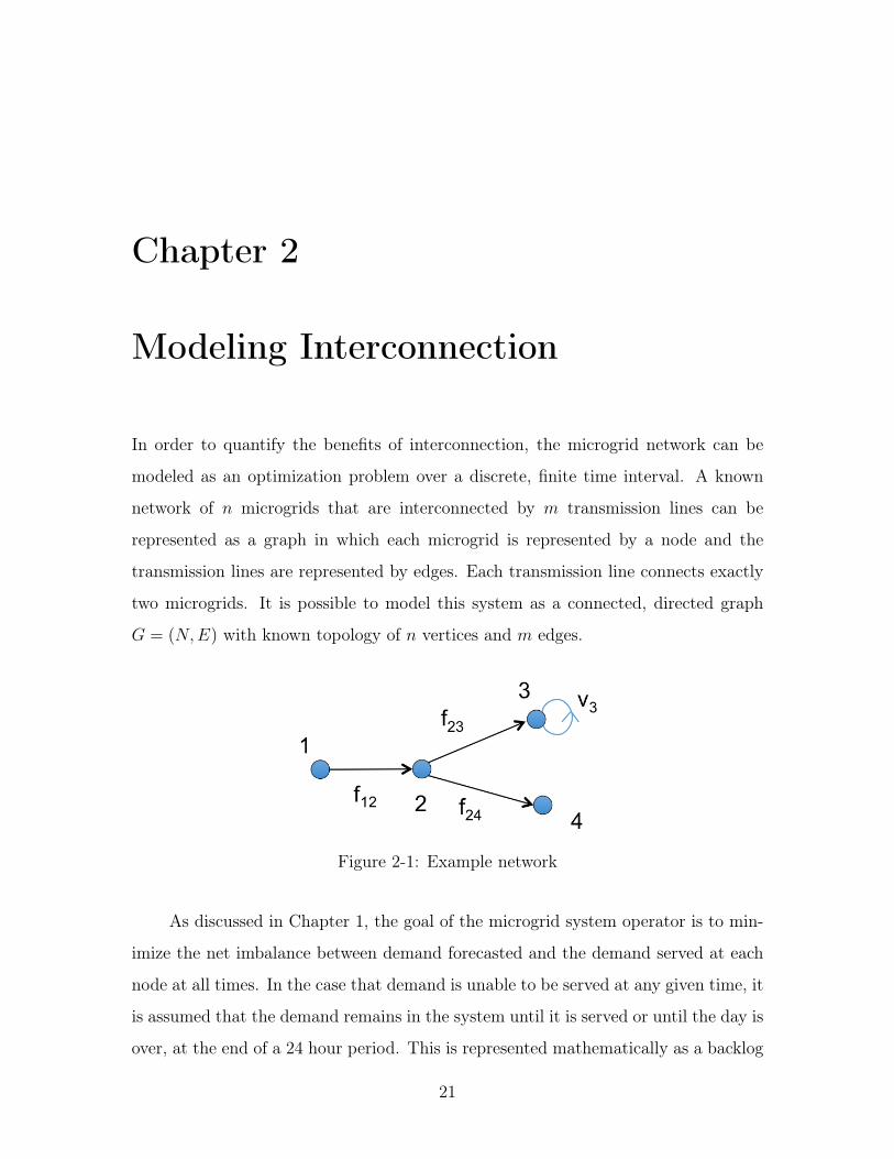
In order to quantify the benefits of interconnection, the microgrid network can be
modeled as an optimization problem over a discrete, finite time interval. A known
network of 𝑛 microgrids that are interconnected by 𝑚 transmission lines can be
represented as a graph in which each microgrid is represented by a node and the
transmission lines are represented by edges. Each transmission line connects exactly
two microgrids. It is possible to model this system as a connected, directed graph
𝐺 = (𝑁,𝐸) with known topology of 𝑛 vertices and 𝑚 edges.
Figure 2-1: Example network
As discussed in Chapter 1, the goal of the microgrid system operator is to min-
imize the net imbalance between demand forecasted and the demand served at each
node at all times. In the case that demand is unable to be served at any given time, it
is assumed that the demand remains in the system until it is served or until the day is
over, at the end of a 24 hour period. This is represented mathematically as a backlog
21

state. The cost function has two terms in it. Costs are associated with the backlog of
unmet demand and transmitting energy between microgrids across the transmission
lines. The cost of backlog is quadratic so that larger deviations are penalized more
heavily
We keep track of two states. The first state, 𝑥(𝑡) ∈ R𝑛 is a vector recording
the total imbalance between energy served and energy demanded at every node. The
imbalanced is backlogged, with a negative balance implying that there is unserved
demand from earlier time periods. We require state 𝑥 to be less than or equal to
zero at all times which ensures that demand is not over-served. The second state is
a vector of battery states 𝑏(𝑡) ∈ R𝑛 at each node at time t, which tracks the amount
of storage available at each node 𝑖. Each battery is limited by its maximum capacity
and a positivity constraint.
We assume that we have some forecasted exogenous supply and demand, where
𝑑𝑖(𝑡) represents aggregate local demand at node 𝑖 and 𝑠𝑖(𝑡) is aggregate local supply at
node 𝑖. Supply and demand forecasts are assumed to be given as positive values. Our
decisions at every time point 𝑡 are 𝑣𝑖(𝑡): how much demand to serve locally, as well as
𝑓𝑖𝑗(𝑡) ∀(𝑖, 𝑗) ∈ 𝐸: the amount of energy to be traded with other microgrids in the
network through the links. The demand served is constrained to be positive so as not
to allow for the battery to draw energy back from the consumers. The flow variables,
or amount of energy exchanged with the network at each node, are subject to the
capacity constraints of the transmission line and to network flow conservation. In
the directed graph, negative flow implies that energy is flowing against the direction
of the link (for example 𝑓23 ≤ 0 implies that energy flows from node 3 to node 2 in
Figure 2-1). Thus the model is formulated as follows:
min𝑣𝑖,𝑓𝑖𝑗
∑︁𝑖∈𝑁
𝑇∑︁𝑡=1
𝑄𝑖𝑥2𝑖 (𝑡) +
∑︁(𝑖,𝑗)∈𝐸
𝑇−1∑︁𝑡=1
𝑅𝑖𝑗𝑓2𝑖𝑗(𝑡) (2.1)
subject to:
𝑥𝑖(𝑡+ 1) = 𝑥𝑖(𝑡) + 𝑣𝑖(𝑡)− 𝑑𝑖(𝑡) (2.2)
22
𝑏𝑖(𝑡+ 1) = 𝑏𝑖(𝑡) +∑︁𝑗∈𝐼(𝑖)
𝑓𝑗𝑖(𝑡)−∑︁
𝑗∈𝑂(𝑖)
𝑓𝑖𝑗(𝑡)− 𝑣𝑖(𝑡) + 𝑠𝑖(𝑡) (2.3)
𝑣𝑖(𝑡) ≥ 0 (2.4)
𝑥𝑖(𝑡) ≤ 0 (2.5)
𝑏𝑖(𝑡) ≥ 0 (2.6)
𝑏𝑖(𝑡) ≤ 𝑏𝑚𝑎𝑥 (2.7)
−𝑐 ≤ 𝑓𝑖𝑗(𝑡) ≤ 𝑐 (2.8)
Note that the battery state 𝑏𝑖(𝑡) has no cost associated with it. The role of the
battery is to provide flexibility in our decision making at each time point. While
decision variables 𝑣𝑖(𝑡) are not explicitly upper-bounded, the lower bound on battery
state 𝑏𝑖 serves to dynamically provide a maximum for the energy available at time 𝑡.
We can describe our system in a more compact form by defining new variables
�̃�, 𝑢, and 𝑤:
�̃�(𝑡) = [𝑥1(𝑡) 𝑏1(𝑡) ... 𝑥𝑁(𝑡) 𝑏𝑁(𝑡)]⊤
𝑢(𝑡) = [𝑣1(𝑡) ... 𝑣𝑁(𝑡) 𝑓𝑖𝑗(𝑡)]⊤
𝑤(𝑡) = [𝑑1(𝑡) 𝑠1(𝑡) ... 𝑑𝑁(𝑡) 𝑠𝑁(𝑡)]⊤
Our problem can now be written:
min𝑢
�̃�(𝑇 )⊤𝑄�̃�(𝑇 ) +𝑇−1∑︁𝑡=1
{�̃�(𝑡)⊤𝑄�̃�(𝑡) + 𝑢(𝑡)⊤𝑅𝑢(𝑡)} (2.9)
subject to:
�̃�(𝑡+ 1) = 𝐴�̃�(𝑡) + �̂�𝑢(𝑡) + 𝑤(𝑡) (2.10)
𝐷�̃�(𝑡)− 𝛾 ≤ 0
𝑢 ∈ U
23

Define
𝐷𝑖 =
⎡⎢⎢⎢⎣1 0
0 −1
0 1
⎤⎥⎥⎥⎦𝑄 =
⎡⎣1 0
0 0
⎤⎦ , 𝛾 =
⎡⎢⎢⎢⎣0
0
−𝑏𝑚𝑎𝑥
⎤⎥⎥⎥⎦then D is the block diagonal matrix with blocks 𝐷𝑖 and 𝛾 = [𝛾𝑖]
⊤ for 𝑖 = 1...𝑁 . 𝐴 is
block diagonal matrix of [2× 2] identity vectors, 𝑅 is a diagonal matrix with entry 1
for 𝑓𝑖𝑗 and 0 for 𝑣𝑖, and �̂� is the matrix of decision variable coefficients.
2.1 Constrained LQR
The linear quadratic regulator is a well studied dynamic programming problem. It
refers to the optimization of a linear dynamic system over a quadratic cost function
𝐽(𝑥𝑡, 𝑢𝑡):
𝐽(𝑥𝑡, 𝑢𝑡) = min𝑢
E𝑤𝑡{𝑥(𝑇 )⊤𝑄𝑥(𝑇 ) +𝑇−1∑︁𝑡=0
𝑥⊤(𝑡)𝑄𝑥(𝑡) + 𝑢⊤(𝑡)𝑅𝑢(𝑡)}
subject to: 𝑥(𝑡+ 1) = 𝐴𝑥(𝑡) +𝐵𝑢(𝑡) + 𝑤(𝑡)
where matrix 𝑄 is assumed to be positive semi-definite and 𝑅 is positive definite,
and the expected value of disturbances 𝑤 is assumed to be zero. In the case of a
linear quadratic system with no other constraints, it is possible to find an analytical
solution even under uncertain conditions [28]. The optimal control 𝜇𝑡(𝑥𝑡) is found to
be linear in 𝑥 with the form
𝜇𝑡(𝑥𝑡) = 𝐿𝑡𝑥𝑡
where 𝐿𝑡 is determined by solving the discrete time Ricatti equation
𝐿𝑡 = −(𝐵⊤𝐾𝑡+1𝐵 +𝑅)−1𝐵⊤𝐾𝑡+1𝐴
with 𝐾 defined as
𝐾𝑡 = 𝑄+ 𝐴⊤𝐾𝑡+1𝐴− 𝐴⊤𝐾𝑡+1𝐵(𝑅 +𝐵⊤𝐾𝑡+1𝐵)−1𝐵⊤𝐾𝑡+1𝐴
24
and the optimal cost is given by:
𝐽0(𝑥0) = 𝑥⊤0 𝐾0𝑥0 +
𝑇−1∑︁𝑡=0
E{𝑤⊤𝑡 𝐾𝑡+1𝑤𝑡} [28]
Our problem formulation given in Equation 2.9 is similar to the well studied
linear-quadratic regulator (LQR) problem, in that we are minimizing a quadratic
cost function of a system whose dynamics are described by a linear time invariant
system. However, the optimization problem presented in Equation 2.1 has key dis-
tinctions. First, the addition of even simple constraints destroys the structure of
the Ricatti equation, and can quickly make the classical dynamic programming ap-
proach computationally intractable [29]. Second, matrix R in Equation 2.9 is positive
semidefinite, not positive definite.
The constrained LQR (CLQR) problem has also been studied extensively for
deterministic problems. Given the deterministic CLQR problem:
𝐽(𝑥𝑡, 𝑢𝑡) = min𝑢
𝑥(𝑇 )⊤𝑄𝑥(𝑇 ) +𝑇−1∑︁𝑡=0
𝑥⊤(𝑡)𝑄𝑥(𝑡) + 𝑢⊤(𝑡)𝑅𝑢(𝑡)
subject to: 𝑥(𝑡+ 1) = 𝐴𝑥(𝑡) +𝐵𝑢(𝑡) + 𝑤(𝑡)
𝑢 ∈ 𝑈
It is possible to reformulate the LQR as a quadratic programming problem parametrized
by the initial conditions 𝑥𝑜 [30]. This can be shown directly by defining matrices:
𝑥 =
⎡⎢⎢⎢⎣�̃�(1)
...
�̃�(𝑇 )
⎤⎥⎥⎥⎦ , 𝑢 =
⎡⎢⎢⎢⎣𝑢(1)
...
𝑢(𝑇 )
⎤⎥⎥⎥⎦ , 𝑤 =
⎡⎢⎢⎢⎣𝑤(1)
...
𝑤(𝑇 )
⎤⎥⎥⎥⎦
𝐹 =
⎡⎢⎢⎢⎣𝐴...
𝐴𝑇
⎤⎥⎥⎥⎦ , 𝐻 =
⎡⎢⎢⎢⎢⎢⎢⎣𝐵
𝐴𝐵 𝐵... · · · . . .
𝐴𝑇−1𝐵 𝐴𝑇−2𝐵 · · · 𝐵
⎤⎥⎥⎥⎥⎥⎥⎦ ,
25
�̃� =
⎡⎢⎢⎢⎣𝑄
. . .
𝑄
⎤⎥⎥⎥⎦ , �̃� =
⎡⎢⎢⎢⎣𝑅
. . .
𝑅
⎤⎥⎥⎥⎦Re-writing the LQR in terms of 𝐹 , 𝐻, �̃�, and �̃�, one can equivalently write the
problem as:
min𝑢
𝑥⊤𝑜 𝐹
⊤�̃�𝐹𝑥𝑜 + 2𝑥⊤𝑜 𝐹
⊤�̃�𝐻𝑢+ 𝑢⊤(�̃� +𝐻⊤�̃�𝐻)𝑢
subject to: 𝑢 ∈ 𝑈
Therefore, the CLQR problem can also be formulated as a quadratic program over
some constraint set, and solved explicitly given some initial value 𝑥0 [31, 32]. Be-
mporad et al. extended this to show that for any initial value, the CLQR can be
formulated as a multi-parametric quadratic program and solved for all 𝑥0 within a
polyhedral set of values, leading to a piece-wise affine optimal control policy [33].
2.2 Centralized Solution
Instead of taking the dynamic programming approach, the problem can be formulated
as a Quadratic Program (QP). Given initial values 𝑥0 and 𝑏0 at every node and known
supply and demand forecasts, backlog state 𝑥𝑖 and battery state 𝑏𝑖, as defined by
equations 2.2 and 2.3, can each be explicitly written as T static constraints. Define
vectors 𝑥𝑖 and 𝑏𝑖:
𝑥𝑖 =
⎡⎢⎢⎢⎣𝑥𝑖(1)
...
𝑥𝑖(𝑇 )
⎤⎥⎥⎥⎦ , 𝑏𝑖 =
⎡⎢⎢⎢⎣𝑏𝑖(1)
...
𝑏𝑖(𝑇 )
⎤⎥⎥⎥⎦26
Also, define L as the T*T lower triangular matrix of ones:
𝐿 =
⎡⎢⎢⎢⎢⎢⎢⎣1
1 1... · · · . . .
1 1 · · · 1
⎤⎥⎥⎥⎥⎥⎥⎦Then
𝑥𝑖 = 1⃗𝑥0 + 𝐿(𝑣𝑖 − 𝑑𝑖) (2.11)
𝑏𝑖 = 1⃗𝑏0 + 𝐿(−𝑣𝑖 + 𝑠𝑖 −∑︁
𝑗∈𝑂(𝑖)
𝑓𝑖𝑗 +∑︁𝑗∈𝐼(𝑖)
𝑓𝑗𝑖) (2.12)
where each 𝑣𝑖 and 𝑓𝑖𝑗 are [(𝑇 − 1)x1] vectors:
𝑣𝑖 = [𝑣𝑖(1) 𝑣𝑖(2) ... 𝑣𝑖(𝑇 − 1)]⊤
𝑓𝑖𝑗 = [𝑓𝑖𝑗(1) 𝑓𝑖𝑗(2) ... 𝑓𝑖𝑗(𝑇 − 1)]⊤
Therefore, the model is written as:
min𝑣,𝑓𝑖𝑗
∑︁𝑖∈𝑁
𝑥⊤𝑖 𝑄𝑖𝑥𝑖 +
∑︁(𝑖,𝑗)∈𝐸
𝑓⊤𝑖𝑗𝑅𝑖𝑗𝑓𝑖𝑗 (2.13)
subject to:
𝑥𝑖 = 1⃗𝑥0 + 𝐿(𝑣𝑖 − 𝑑𝑖) (2.14)
𝑏𝑖 = 1⃗𝑏0 + 𝐿(−𝑣𝑖 + 𝑠𝑖 −∑︁
𝑗∈𝑂(𝑖)
𝑓𝑖𝑗 +∑︁𝑗∈𝐼(𝑖)
𝑓𝑗𝑖) (2.15)
𝑣𝑖 ≥ 0 (2.16)
𝑥𝑖 ≤ 0 (2.17)
𝑏𝑖 ≥ 0 (2.18)
𝑏𝑖 ≤ 𝑏𝑖𝑚𝑎𝑥 (2.19)
27

−𝑐 ≤ 𝑓𝑖𝑗 ≤ 𝑐 (2.20)
This problem formulation can be solved online with a QP solver for a finite period of
time T.
2.3 Discussion and Simulations
The value of microgrid interconnection relies on the heterogeneity of the network.
Realistically, neighboring microgrids in off-grid India will be faced with very similar
supply and demand distributions. Thus, it is reasonable to assume that the supply
and demand forecasts at each microgrid will be highly correated, and therefore be
drawn from the same distribution 𝑠𝑖 ∈ 𝑠𝑜 and 𝑑𝑖 ∈ 𝑑𝑜. However, one way in which to
ensure that the network is not homogenous is to vary the amount of storage capacity
at each microgrid.
For the simulations, solar data was retrieved from the National Renewable En-
ergy Laboratory (NREL) from Ranchi, India from January through December. An
aggregate demand load profile was generated from information was collected from 5
residential households which had access to a cell charger, two LED light bulb, and
a fan [34]. To generate multiple forecasts to use at each node, a random offset was
(a) Annual Power Output of 250 W Solar Panel,Ranchi, India
(b) Aggregated Demand, 5 households
Figure 2-2: Supply and Demand Data
28

added to the original distribution by sampling from a scaled uniform distribution with
zero mean 𝑟 ∈ R(−.5, .5). Call the original supply and demand forecasts 𝑠𝑜 and 𝑑𝑜
respectively, then:
𝑠𝑖 = 𝑠𝑜 + 𝑟𝑖 * 𝑠𝑜
𝑑𝑖 = 𝑑𝑜 + 𝑟𝑖 * 𝑑𝑜
Typical offsets can be seen in Figure 2-3.
(a) Randomly Offset Supply (b) Randomly Offset Demand
Figure 2-3
2.3.1 Centralized Simulations
Simulations are used to assess the benefits of interconnection under varied circum-
stances. In each simulation, the optimization period is over 24 hours. The optimiza-
tion is run each day, then at the end of each day backlog is forgiven but battery
state is remembered. There is one case in which the model can become infeasible:
if there is excess generation capacity and the battery is full, the model will become
infeasible. To overcome this issue, a decision to “spill” energy can be added to the
battery constraint:
𝑏𝑖(𝑡+ 1) = 𝑏𝑖(𝑡) +∑︁𝑗∈𝐼(𝑖)
𝑓𝑗𝑖(𝑡)−∑︁
𝑗∈𝑂(𝑖)
𝑓𝑖𝑗(𝑡)− 𝑣𝑖(𝑡) + 𝑠𝑖(𝑡)− 𝑠𝑝𝑖𝑙𝑙𝑖(𝑡)
29
where spill is always positive. This would be avoided unless where entirely necessary
by adding a significantly large penalty in the cost term. For the simulations, spill
with linearly penalized with a coefficient of 100, 000.
There are two reasons why the microgrid system may become strained. First,
upon inspection of the data it is clear that there is a surge in power usage from
Month 2 through Month 7 when the temperature is higher. The upsurge in power
consumption is mostly attributed to the use of fan, which are assumed to turn on after
reaching an ambient temperature of 32∘ Celsius in the load profile generation [34].
The system can be sized such that this power usage is taken into account, or it can
be sized to only serve “critical” demand, which in this case refers to LED lighting and
cell phone charging.
Often solar microgrids being implemented in India are sized to support small,
critical loads (See Section 1.3). For example, microgrid companies such as Mera
Gao would outfit a village of 25-30 households with a 240W capacity solar panel.
A small microgrid like this would generally be supported with a 12V, 100-150Ahr
battery. Transmission line capacity is dependent on a series of factors that are cable
dependent. Antoniou et. al analyzes low voltage DC distribution networks, including
an analysis of total power capacity of 3-core cables under various DC configurations.
The lowest total power for a DC unipolar cable was 61 kW [35]. We conservatively
set the maximum transmission between the microgrids at 10 kW. Let 𝑄 be the 𝑛x𝑛
and and 𝑅 be the 𝑚x𝑚 identity matrices.
For the simulations, the supply data is taken directly from the 250W solar panel
output data. This is roughly equivalent to the size of microgrids currently being
implemented in rural India. The demand data is multiplied by five to represent
aggregate load of 25 households, which is the size of a typical small microgrid, then
an offset is added at each microgrid, as described above. Aggregate supply and
demand for the year are shown in Figure 2-4.
30

Figure 2-4: Aggregate Annual Supply and Demand Profile for 25 Households, 250WSolar Panel
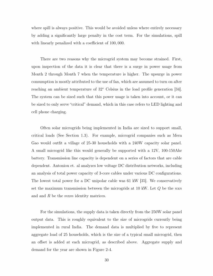
Network Effects and Battery Placement
First we are interested in studying the effect of the network on the optimization
results. As mentioned above, a realistic way to introduce heterogeneity into the
network is through battery placement strategies. Here, we evaluate the impact of
the location of batteries with respect to the network topology to identify the impact
of relative position of microgrids with and without storage capacity. We assess the
impact using a linear network of 20 microgrids, shown in Figure 2-5a. First, storage is
increased from 0 Whr capacity to 72,000 Whr capacity (equivalent to 20 12V, 100Ahr
batteries), but the battery bank is always placed at the end of the network (Node 1
- red). Second, batteries are placed in the middle of the network (Node 10 - green).
Finally, batteries are distributed throughout the network, with 1200 Whr at each
node with a battery. Results are shown in Figure 2-5.
This is an example of how the heterogeneity of the nodes in relation to the
topology of the network has consequence. By placing the batteries at the end of the
network, not only does average performance decrease overall, but power is distributed
31
(a) 20 Node Network (b) Reliability Over Time - Dif-ferent Battery Configurations
(c) Nodal Demand Served,3000 Whr Total Storage Ca-pacity
Figure 2-5: Impact of Battery Placement, Linear Network
less equitably. Figure 2-5c shows the disparity in demand served nodally given equal
sized capacity distributed either at the end or evenly throughout the network. De-
mand at the nodes further from the batteries will only be served until the costs of
transmission outweigh the costs of backlog. This can be explored further with an
extreme case.
Say there are only two nodes on the system. We examine the extreme case in
which Node 1 has an abundance of supply (𝑠1 >> 𝑑1, 𝑏𝑚𝑎𝑥 = ∞) and a very large
storage bank, while Node 2 has constrained supply (∑︀𝑇
𝑡=1(𝑠2(𝑡) − 𝑑2(𝑡) < 0) and no
storage capacity. Following from Equation 2.13, the cost function can be written as:
min𝑓12,𝑣1,𝑣2
𝑥⊤1 𝑄1𝑥1 + 𝑥⊤
2 𝑄2𝑥22 + 𝑓⊤
12𝑅12𝑓12
where
𝑥𝑖 = 1⃗𝑥0 + 𝐿(𝑣𝑖 − 𝑑𝑖) (2.21)
Plugging in from 2.21 for 𝑥1 and 𝑥2, and assuming 𝑥0 = 0 for both microgrids we
have:
min𝑓12,𝑣1,𝑣2
(𝑣1 − 𝑑1)⊤𝐿⊤𝑄1𝐿(𝑣1 − 𝑑1) + (𝑣2 − 𝑑2)
⊤𝐿⊤𝑄2𝐿(𝑣2 − 𝑑2) + 𝑓⊤12𝑅12𝑓12
32
subject to:
𝐿(𝑣1 − 𝑑1) ≤ 0 (2.22)
𝐿(𝑣2 − 𝑑2) ≤ 0 (2.23)
𝑏1 = 1⃗𝑏0 + 𝐿(−𝑣1 + 𝑠1 − 𝑓12) (2.24)
0 = −𝑣2 + 𝑠2 + 𝑓12 (2.25)
𝑣1 ≥ 0 (2.26)
𝑣2 ≥ 0 (2.27)
−𝑐 ≤ 𝑓12 ≤ 𝑐 (2.28)
For convenience, define new variable 𝑣𝑖 = 𝑣𝑖 − 𝑑𝑖
Under the assumptions that 𝑠1 >> 𝑑1, and 𝑏𝑚𝑎𝑥 = ∞, the battery constraint
on Node 1, Equation 2.24, is not active. Let us also assume that the congestion
constraint is not active. Without the active battery constraint, the optimization over
𝑣1 is separable, and can be found to optimally be 𝑑1 for all time points. This leaves
us with decisions 𝑓12 and demand to serve at Node 2 𝑣2.
min𝑓12,𝑣2
𝑣⊤2 𝐿⊤𝑄2𝐿𝑣2 + 𝑓⊤
12𝑅12𝑓12
subject to:
𝐿𝑣2 ≤ 0
0 = −𝑣2 + 𝑠2 − 𝑑2 + 𝑓12
−𝑣2 + 𝑑2 ≤ 0
Replacing 𝑣2 with the equality constraint 𝑣2 = 𝑠2 − 𝑑2 + 𝑓12 and taking the
gradient with respect to decision variables 𝑓12:
2𝐿⊤𝑄2𝐿(𝑠2 − 𝑑2 + 𝑓12) + 2𝑅12𝑓12
33

Applying KKT Conditions where 𝜇 ≥ 0:
−𝐿⊤𝑄2𝐿(𝑠2 − 𝑑2 + 𝑓12)−𝑅12𝑓12 =1
2(𝜇1𝐿− �⃗�2)
𝑓12 = −(𝐿⊤𝑄2𝐿+𝑅12)−1(
1
2(𝜇1𝐿− �⃗�2) + 𝐿⊤𝑄2𝐿(𝑠2 − 𝑑2))
In the extreme case that 𝑠2 − 𝑑2 is always negative, for example if 𝑠2 = 0, then
the negativity constraint is not active at the optimal solution, and we have:
𝑓12 = (𝐿⊤𝑄2𝐿+𝑅12)−1(𝐿⊤𝑄2𝐿𝑑2)
The impact of the network is captured in the cost of transmitting energy between
the microgrids. There is a trade-offf when removing local resources in favor of a
networked system; the overall system costs may be reduced, but individual microgrids
whose utilities are locally defined only by unmet backlog could suffer. This stresses
the importance of tuning the parameters Q and R to reflect the value of microgrids.
In this example, in the case that backlog is weighted very heavily, ie 𝑄2 >> 𝑅12, then
all demand can be served. However, the larger the relative cost of transmission, the
less demand will be served despite the generation capacity to do so.
Performance As a Function of Batteries in Network
Microgrid interconnection has the potential to lessen the need for on-site storage
throughout the network. In this section, different storage capacities are compared for
varying microgrid networks. Battery capacity is measured by total capacity in Whr,
or by “battery saturation,” which we define by the number of microgrids that are
outfitted with a 12V 100Ahr battery out of the total number of microgrids. Batteries
are placed such that they have an equal number of nearest nodes without batteries at
an equal distance. For the initial analysis, Month 7 is used as a representative month
in which the system is strained (during the end of monsoon season) but without an
excess of non-critical load.
To test the effects of battery saturation directly, six graphs are simulated with
34

various battery saturations (see Figure 2-7). There was little difference between the
network configurations because batteries were dispersed throughout the network. In
each situation, there were some clear trends. First, the value of interconnection first
increases then decreases in number of batteries removed from the network. Second,
and importantly, the overall reliability of the network does not immediately decrease.
This implies that the storage capacity at each microgrid is not being fully utilized.
Therefore, until a certain point, microgrid interconnection can replace physical bat-
teries in the network without significantly retracting from reliability.
(a) Network 1 (b) Network 2 (c) Network 3
(d) Network 4 (e) Network 5 (f) Network 6
Figure 2-6: Microgrid Networks Compared
Year-round Simulations
As shown above, batteries that are evenly dispersed throughout a network will perform
comparably. Thus, for the remaining analysis we use the 10-node linear network
(Network 6). In this section, the same analysis is performed on the 10-node linear
network over the course of the entire year. Simulating over the entire year includes
more demand side variance because of the high levels of non-critical fan loads during
hotter months. Figure 2-8 shows that even with high demand variance, a 40% decrease
35
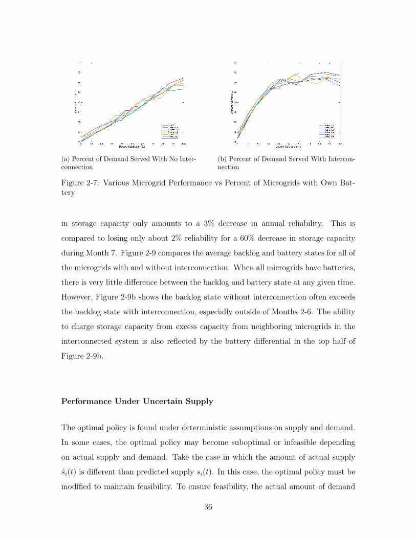
(a) Percent of Demand Served With No Inter-connection
(b) Percent of Demand Served With Intercon-nection
Figure 2-7: Various Microgrid Performance vs Percent of Microgrids with Own Bat-tery
in storage capacity only amounts to a 3% decrease in annual reliability. This is
compared to losing only about 2% reliability for a 60% decrease in storage capacity
during Month 7. Figure 2-9 compares the average backlog and battery states for all of
the microgrids with and without interconnection. When all microgrids have batteries,
there is very little difference between the backlog and battery state at any given time.
However, Figure 2-9b shows the backlog state without interconnection often exceeds
the backlog state with interconnection, especially outside of Months 2-6. The ability
to charge storage capacity from excess capacity from neighboring microgrids in the
interconnected system is also reflected by the battery differential in the top half of
Figure 2-9b.
Performance Under Uncertain Supply
The optimal policy is found under deterministic assumptions on supply and demand.
In some cases, the optimal policy may become suboptimal or infeasible depending
on actual supply and demand. Take the case in which the amount of actual supply
𝑠𝑖(𝑡) is different than predicted supply 𝑠𝑖(𝑡). In this case, the optimal policy must be
modified to maintain feasibility. To ensure feasibility, the actual amount of demand
36

(a) Month 7 (b) All Year
Figure 2-8: Percent of Demand Served vs Storage Capacity for Network 6
(a) 10 Batteries
(b) 6 Batteries
Figure 2-9: Network 6 Backlog and Battery State Over Time
served locally 𝑣𝑖(𝑡) can be adjusted at any given time:
𝑣𝑖(𝑡) = min(𝑣𝑖(𝑡), 𝑏𝑖(𝑡− 1) +𝐵𝑖𝑢*(𝑡) + 𝑠𝑖(𝑡))
37
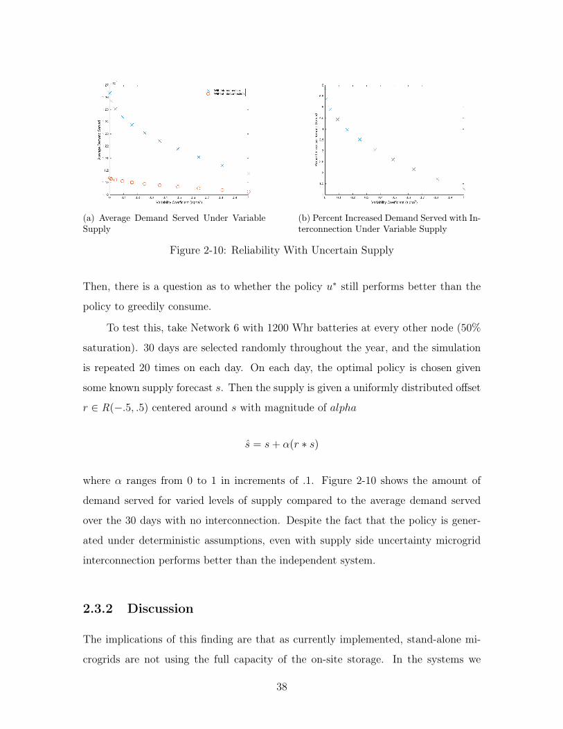
(a) Average Demand Served Under VariableSupply
(b) Percent Increased Demand Served with In-terconnection Under Variable Supply
Figure 2-10: Reliability With Uncertain Supply
Then, there is a question as to whether the policy 𝑢* still performs better than the
policy to greedily consume.
To test this, take Network 6 with 1200 Whr batteries at every other node (50%
saturation). 30 days are selected randomly throughout the year, and the simulation
is repeated 20 times on each day. On each day, the optimal policy is chosen given
some known supply forecast 𝑠. Then the supply is given a uniformly distributed offset
𝑟 ∈ R(−.5, .5) centered around 𝑠 with magnitude of 𝑎𝑙𝑝ℎ𝑎
𝑠 = 𝑠+ 𝛼(𝑟 * 𝑠)
where 𝛼 ranges from 0 to 1 in increments of .1. Figure 2-10 shows the amount of
demand served for varied levels of supply compared to the average demand served
over the 30 days with no interconnection. Despite the fact that the policy is gener-
ated under deterministic assumptions, even with supply side uncertainty microgrid
interconnection performs better than the independent system.
2.3.2 Discussion
The implications of this finding are that as currently implemented, stand-alone mi-
crogrids are not using the full capacity of the on-site storage. In the systems we
38

simulated, giving each system a 12V, 100 Ahr battery provides excess capacity. This
storage capability could instead be replaced by interconnection with a network of
existing microgrids. Whether or not a small microgrid should be outfitted with a
battery would depend on the exact network configuration of the microgrid network,
and which microgrids already had batteries. Overall, microgrid interconnection was
shown to provide value even for microgrids that are near by and would have highly
correlated supply and demand. During Month 7 when the demand was mostly crit-
ical load and supply was reduced due to monsoon season, it was possible to remove
storage capacity from 6/10 of the microgrids with only a %2 reduction in reliability.
This means that for microgrids that are sized to serve critical demand, just 40% of
the microgrids could be outfitted with batteries without significantly detracting from
reliability of critical load. Simulating over the entire year which included both crit-
ical and non-critical load, Figure 2-8 shows that even with high demand variance, a
40% decrease in storage capacity only amounts to a 3% decrease in annual reliability.
Depending on the sizing and types of load on the system, microgrid networks could
greatly reduce the total number of storage devices system-wide.
39

40

Chapter 3
Layered Optimization for Local
Implementation
The centralized approach gives a sense of the value that microgrid interconnection
can bring to a network of nearby villages. This problem can be directly solved via a
centralized optimization as long as the controller has access to full information across
all microgrids. However, it is often the case that microgrids would not have full ac-
cess to each other’s information for privacy or communication reasons. Furthermore,
it may be unrealisitc to assume that a centralized controller would exist and that
the other microgrids would be comfortable relinquishing decision making to a single
controller. Because of this we are interested in formulating this problem in a decom-
posed way. The goal is to allow microgrids to retain their own proprietary supply
and demand data, while still participating in the networked system. Instead of one
global optimization, microgrids should make decisions autonomously, then participate
in a marketplace to adjust the response to be globally optimal. To do this, the opti-
mization problem is decomposed into a 2-layer scheme. The local “scheduling” layer
encompasses on-site decision making on the amount of demand to serve locally, and
the second, “congestion” layer ensures the feasibility of the local results by updating
price signals.
41

Figure 3-1: Layered Decomposition
3.1 Dual Decomposition
To compute the optimizations locally, we use a decomposition method known as dual
decomposition. Dual decomposition is a layered optimization technique that relies
on taking the Lagrangian dual of a subset of the constraint set. In general, the
Lagrangian dual is formulated as follows. Given a problem
min𝑢
𝑓0(𝑢)
subject to:
𝑓𝑖(𝑢) ≤ 0 𝑖 = 1, ...,𝑚 (3.1)
ℎ𝑗(𝑢) ≤ 0 𝑗 = 1, ..., 𝑝 (3.2)
To formulate the Lagrangian 𝐿 : R𝑛 × R𝑚 → R with constraint (3.1), introduce
Lagrange multipliers 𝜆𝑖:
𝐿(𝑢, 𝜆) = 𝑓0(𝑢) +𝑚∑︁𝑖=1
𝜆⊤𝑖 𝑓𝑖(𝑢)
Define the Lagrangian dual function 𝑔 : R𝑚 → R
𝑔(𝜆) = min𝑢
𝐿(𝑢, 𝜆) = 𝑓0(𝑢) +𝑚∑︁𝑖=1
𝜆⊤𝑖 𝑓𝑖(𝑢)
subject to: ℎ𝑗(𝑢) ≤ 0 𝑗 = 1, ..., 𝑝
42

The Lagrangian dual function gives us a lower bound on the optimal value of the
original optimization problem [36]. In order to find the best lower bound one then
solves the optimization problem
max𝜆
𝑔(𝜆)
subject to: 𝜆𝑖 ≥ 0 𝑖 = 1, ...,𝑚
In dual decomposition, the cost function of the problem is separable in decision vari-
ables 𝑢, but decisions are coupled by a subset of the constraint set. The Lagrangian
dual is applied to the coupling constraints in order to decompose the problem into in-
dependent subproblems. A secondary, “master” problem then finds the optimal value
for the dual vector. This can be interpreted as the setting of prices for the coupled
resources that are optimized in each subproblem in order to guarantee feasibility of
the primal problem [37].
Upon inspection, it is clear that our model may lend itself to a decomposition
method because the cost function is fully separable in 𝑖. However, the constraints are
coupled by the flow variables 𝑓𝑖𝑗 and 𝑓𝑗𝑖 in Equation 2.3. In order to decompose this
problem, we define a new variable 𝑘𝑗𝑖 where
𝑘𝑗𝑖 = 𝑓𝑗𝑖 ∀𝑗 ∈ 𝐼(𝑖) (3.3)
The problem is now written as:
min𝑣,𝑓𝑖𝑗 ,𝑘
∑︁𝑖∈𝑁
𝑥⊤𝑖 𝑄𝑖𝑥𝑖 +
∑︁𝑗∈𝑂(𝑖)
𝑓⊤𝑖𝑗 �̂�𝑖𝑗𝑓𝑖𝑗 +
∑︁𝑗∈𝐼(𝑖)
𝑘⊤𝑗𝑖�̂�𝑗𝑖𝑘𝑗𝑖 (3.4)
subject to:
𝑥𝑖 = 1⃗𝑥0 + 𝐿(𝑣𝑖 − 𝑑𝑖) (3.5)
𝑏𝑖 = 1⃗𝑏0 + 𝐿(−𝑣𝑖 + 𝑠𝑖 +∑︁𝑗∈𝐼(𝑖)
𝑘𝑗𝑖 −∑︁
𝑗∈𝑂(𝑖)
𝑓𝑖𝑗) (3.6)
𝑣𝑖 ≥ 0 (3.7)
43
𝑥𝑖 ≤ 0 (3.8)
𝑏𝑖 ≥ 0 (3.9)
𝑏𝑖 ≤ 𝑏𝑖𝑚𝑎𝑥 (3.10)
−𝑐 ≤ 𝑓𝑖𝑗 ≤ 𝑐 (3.11)
𝑘𝑗𝑖 = 𝑓𝑗𝑖 ∀𝑗 ∈ 𝐼(𝑖) (3.12)
This problem is completely decomposable except for Equation 3.12. To eliminate
the coupling constraint we formulate the Lagrangian dual problem:
L(𝜆, 𝑣, 𝑓, 𝑘) = max𝜆
min𝑘𝑗𝑖,𝑓𝑖𝑗 ,𝑣𝑖
∑︁𝑖∈𝑁
𝑥⊤𝑖 𝑄𝑖𝑥𝑖+
∑︁𝑗∈𝑂(𝑖)
𝑓⊤𝑖𝑗 �̂�𝑖𝑗𝑓𝑖𝑗+
∑︁𝑗∈𝐼(𝑖)
{𝑘⊤𝑗𝑖�̂�𝑗𝑖𝑘𝑗𝑖+𝜆⊤
𝑗𝑖(𝑘𝑗𝑖−𝑓𝑗𝑖)}
(3.13)
where every 𝜆𝑗𝑖 is a [(𝑇 − 1)× 1] vector:
𝜆𝑗𝑖 = [𝜆𝑗𝑖(1) 𝜆𝑗𝑖(2) ... 𝜆𝑗𝑖(𝑇 − 1)]⊤ ∀𝑗 ∈ 𝐼(𝑖)
Define 𝑔(𝜆) as
𝑔(𝜆) = min𝑘𝑗𝑖,𝑓𝑖𝑗 ,𝑣𝑖
∑︁𝑖∈𝑁
[𝑥⊤𝑖 𝑄𝑖𝑥𝑖 +
∑︁𝑗∈𝑂(𝑖)
𝑓⊤𝑖𝑗 �̂�𝑖𝑗𝑓𝑖𝑗 +
∑︁𝑗∈𝐼(𝑖)
{𝑘⊤𝑗𝑖�̂�𝑗𝑖𝑘𝑗𝑖 + 𝜆⊤
𝑗𝑖(𝑘𝑗𝑖 − 𝑓𝑗𝑖)}] (3.14)
We first compute 𝑔(𝜆) subject to constraints 3.5 through 3.11 to find 𝑓(𝜆) and 𝑘(𝜆).
The master problem is then:
max𝜆
𝑔(𝜆) (3.15)
Equation 3.14 is not yet fully separable. The battery constraint, Equation 3.6, only
contains flow variables 𝑓𝑖𝑗 for all 𝑗 ∈ 𝑂(𝑖), but the cost function is over all flow
variables 𝑓𝑖𝑗 for all (𝑖, 𝑗) ∈ 𝐸.
Proposition 1 𝑔(𝜆) can be fully decoupled across nodes, written as:
𝑔(𝜆) =∑︁𝑖∈𝑁
min𝑓𝑖𝑗∀𝑗∈𝑂(𝑖),𝑘𝑗𝑖∀𝑗∈𝐼(𝑖),𝑣𝑖
[𝑥⊤𝑖 𝑄𝑖𝑥𝑖 + 𝑓⊤
𝑖𝑗 �̂�𝑖𝑗𝑓𝑖𝑗 + 𝑘⊤𝑗𝑖�̂�𝑗𝑖𝑘𝑗𝑖 +𝜆⊤
𝑗𝑖𝑘𝑗𝑖−𝜆⊤𝑖𝑗𝑓𝑖𝑗)] (3.16)
44

Proof: We can show this directly. First, 𝑔(𝜆) can be written as:
𝑔(𝜆) = min𝑘𝑗𝑖,𝑓𝑖𝑗 ,𝑣𝑖
∑︁𝑖∈𝑁
[𝑥⊤𝑖 𝑄𝑖𝑥𝑖 +
∑︁𝑗∈𝑂(𝑖)
𝑓⊤𝑖𝑗 �̂�𝑖𝑗𝑓𝑖𝑗 +
∑︁𝑗∈𝐼(𝑖)
{𝑘⊤𝑗𝑖�̂�𝑗𝑖𝑘𝑗𝑖 + 𝜆⊤
𝑗𝑖(𝑘𝑗𝑖 − 𝑓𝑗𝑖)}]
=∑︁𝑖∈𝑁
min𝑓𝑖𝑗∀𝑗∈𝑂(𝑖),𝑘𝑗𝑖∀𝑗∈𝐼(𝑖)
𝑥⊤𝑖 𝑄𝑖𝑥𝑖 + 𝑓⊤
𝑖𝑗 �̂�𝑖𝑗𝑓𝑖𝑗 + 𝑘⊤𝑗𝑖�̂�𝑗𝑖𝑘𝑗𝑖 + min
𝑘𝑗𝑖,𝑓𝑗𝑖
∑︁𝑖∈𝑁
∑︁𝑗∈𝐼(𝑖)
𝜆⊤𝑗𝑖(𝑘𝑗𝑖 − 𝑓𝑗𝑖)
(3.17)
We can show that the second term can also be written in terms of local decision
variables 𝑓𝑖𝑗 for all 𝑗 ∈ 𝑂(𝑖) and 𝑘𝑗𝑖 for all 𝑗 ∈ 𝐼(𝑖):
min𝑘𝑗𝑖,𝑓𝑗𝑖
∑︁𝑖∈𝑁
∑︁𝑗∈𝐼(𝑖)
(𝜆⊤𝑗𝑖𝑘𝑗𝑖 − 𝜆⊤
𝑗𝑖𝑓𝑗𝑖)
= min𝑘𝑗𝑖,𝑓𝑖𝑗
∑︁𝑖∈𝑁
∑︁𝑗∈𝐼(𝑖)
𝜆⊤𝑗𝑖𝑘𝑗𝑖 −
∑︁𝑖∈𝑁
∑︁𝑗∈𝑂(𝑖)
𝜆⊤𝑖𝑗𝑓𝑖𝑗
=∑︁𝑖∈𝑁
min𝑓𝑖𝑗∀𝑗∈𝑂(𝑖),𝑘𝑗𝑖∀𝑗∈𝐼(𝑖)
𝜆⊤𝑗𝑖𝑘𝑗𝑖 − 𝜆⊤
𝑖𝑗𝑓𝑖𝑗
(3.18)
Putting the two terms together, we have
𝑔(𝜆) =∑︁𝑖∈𝑁
min𝑓𝑖𝑗∀𝑗∈𝑂(𝑖),𝑘𝑗𝑖∀𝑗∈𝐼(𝑖),𝑣𝑖
[𝑥⊤𝑖 𝑄𝑖𝑥𝑖 + 𝑓⊤
𝑖𝑗 �̂�𝑖𝑗𝑓𝑖𝑗 + 𝑘⊤𝑗𝑖�̂�𝑗𝑖𝑘𝑗𝑖 +𝜆⊤
𝑗𝑖𝑘𝑗𝑖−𝜆⊤𝑖𝑗𝑓𝑖𝑗)] (3.19)
This means that each node 𝑖 optimizes its own total “inflow” 𝑘𝑗𝑖(𝑡) and chooses each
“outflow” 𝑓𝑖𝑗(𝑡) based on price variables 𝜆𝑖𝑗 and 𝜆𝑗𝑖, which are communicated from
neighboring microgrids. Note that “inflow” and “outflow” are defined by graph struc-
ture and do not represent power inflow and outflow - each can be either positive or
negative.
Proposition 2 Each entry of the matrix �̂�𝑖𝑗 is equal to one half of the corresponding
entry of the matrix 𝑅𝑖𝑗.
45
Proof: The links of the graph 𝑓𝑖𝑗 can be equivalently written as:
∑︁(𝑖,𝑗)∈𝐸
𝑓⊤𝑖𝑗𝑅𝑖𝑗𝑓𝑖𝑗 =
∑︁𝑖∈𝑁
∑︁𝑗∈𝑂(𝑖)
𝑓⊤𝑖𝑗𝑅𝑖𝑗𝑓𝑖𝑗 =
∑︁𝑖∈𝑁
∑︁𝑗∈𝐼(𝑖)
𝑓⊤𝑗𝑖𝑅𝑖𝑗𝑓𝑗𝑖
=1
2
∑︁𝑖∈𝑁
∑︁𝑗∈𝑂(𝑖)
𝑓⊤𝑖𝑗𝑅𝑖𝑗𝑓𝑖𝑗 +
1
2
∑︁𝑖∈𝑁
∑︁𝑗∈𝐼(𝑖)
𝑓⊤𝑗𝑖𝑅𝑖𝑗𝑓𝑗𝑖 (3.20)
Then if �̂�𝑖𝑗 =12𝑅𝑖𝑗:
∑︁𝑖∈𝑁
∑︁𝑗∈𝑂(𝑖)
𝑓⊤𝑖𝑗 �̂�𝑖𝑗𝑓𝑖𝑗 +
∑︁𝑗∈𝐼(𝑖)
𝑘⊤𝑗𝑖�̂�𝑗𝑖𝑘𝑗𝑖 =
∑︁𝑖∈𝑁
∑︁𝑗∈𝑂(𝑖)
1
2𝑓⊤𝑖𝑗𝑅𝑖𝑗𝑓𝑖𝑗 +
∑︁𝑗∈𝐼(𝑖)
𝑘⊤𝑗𝑖
1
2𝑅𝑗𝑖𝑘𝑗𝑖 (3.21)
Since 𝑘𝑗𝑖 = 𝑓𝑗𝑖 for all 𝑗 ∈ 𝐼(𝑖), Equation 3.21 is equivalent to Equation 3.20.
3.2 Notes on the Lagrangian
3.2.1 Existence of a Unique Solution
A generic quadratic function 𝑓(𝑥) = 1/2𝑥⊤𝑃𝑥+ 𝑞⊤𝑥+ 𝑟 is strictly convex if and only
if the matrix P is positive defintie (𝑃 ≻ 0) [36]. We show here that both the dual and
primal problem are strictly convex. Recall that the primal cost function is given by
min𝑣𝑖,𝑓𝑖𝑗
∑︁𝑖∈𝑁
𝑥⊤𝑖 𝑄𝑖𝑥𝑖 +
∑︁(𝑖,𝑗)∈𝐸
𝑓⊤𝑖𝑗𝑅𝑖𝑗𝑓𝑖𝑗
where 𝑅𝑖𝑗 > 0 and 𝑄𝑖 > 0. We can plug in 𝑥𝑖 defined by
𝑥𝑖 = 1⃗𝑥0 + 𝐿(𝑣𝑖 − 𝑑𝑖)
to formulate the cost function in terms of 𝑥0:
min𝑣,𝑓𝑖𝑗
∑︁𝑖∈𝑁
𝑇𝑥20 + (𝑣𝑖 − 𝑑𝑖)
⊤𝐿⊤𝐿(𝑣𝑖 − 𝑑𝑖) + 2�⃗�0𝐿(𝑣𝑖 − 𝑑𝑖) +∑︁
(𝑖,𝑗)∈𝐸
𝑓⊤𝑖𝑗𝑅𝑖𝑗𝑓𝑖𝑗 (3.22)
46

Redefine 𝑣𝑖 = 𝑣𝑖 − 𝑑𝑖 and define decision vector
𝑢(𝑡) = [𝑣1(𝑡) ... 𝑣𝑁(𝑡) 𝑓𝑖𝑗(𝑡)]⊤
Then we have
𝑓(𝑢) = min𝑢
𝑇𝑥20 + 𝑢𝐻𝑢+ 2⃗1𝑥0𝐹𝑢 (3.23)
where H as the positive definite block diagonal matrix with
𝐻 =
⎡⎢⎢⎢⎢⎢⎢⎣𝐿⊤𝐿
. . .
𝐿⊤𝐿
𝑅
⎤⎥⎥⎥⎥⎥⎥⎦with 𝑛 𝐿⊤𝐿 blocks, and where R is an 𝑚x𝑚 diagonal matrix of 𝑅𝑖𝑗. This implies the
cost function 𝑓(𝑢) is strongly convex.
The decomposed problem is also strongly convex. In section 3, we decomposed
the problem by adding new variables 𝑘𝑗𝑖(𝑡) = 𝑓𝑗𝑖(𝑡) for all outgoing links 𝑗 ∈ 𝐼(𝑖). As
shown in Equation 3.20, �̂� = 12𝑅, so the cost function can be equivalently written as
∑︁𝑖∈𝑁
min𝑣,𝑓𝑖𝑗∀𝑗∈𝑂(𝑖),𝑘𝑗𝑖∀𝑗∈𝐼(𝑖)
𝑇*𝑥20+(𝑣𝑖−𝑑𝑖)⊤𝐿⊤𝐿(𝑣𝑖−𝑑𝑖)+
1
2𝑓⊤𝑖𝑗𝑅𝑖𝑗𝑓𝑖𝑗+
1
2𝑘⊤𝑗𝑖𝑅𝑖𝑗𝑘𝑗𝑖+2⃗1𝑥0𝐿(𝑣𝑖−𝑑𝑖)
(3.24)
Define decision vector at each node:
𝑢𝑖 = [𝑣𝑖 𝑓𝑖𝑗 𝑘𝑗𝑖]⊤
Re-write the cost in terms of decision vectors 𝑢𝑖:
𝑓𝑑(𝑢) =∑︁𝑖∈𝑁
min𝑢𝑖
𝑇𝑥20 + 𝑢𝑖𝐻𝑖𝑢𝑖 + 2⃗1𝑥0𝐹𝑖𝑢𝑖 (3.25)
47

where u is a vector of vectors 𝑢𝑖 and 𝐻𝑖 is the positive definite block diagonal matrix
𝐻𝑖 =
⎡⎢⎢⎢⎢⎢⎢⎣𝐿⊤𝐿
12𝑅𝑖𝑗
. . .12𝑅𝑗𝑖
⎤⎥⎥⎥⎥⎥⎥⎦Therefore, the decomposed problem 𝑓𝑑(𝑢) is strongly convex.
3.2.2 Strong Duality
We show strong duality between the primal, centralized optimization problem and the
Lagrangian dual problem. In general, the Lagrangian dual may have some positive
valued duality gap 𝑝* − 𝑑*.
Proposition 3 For our Lagrangian dual decomposition defined in Equation 3.13, the
optimal duality gap between the primal optimal solution and the dual optimal solution
is zero: 𝑑* = 𝑝*
Proof: Recall from equation 3.13 that the Lagrangian dual problem is a function of
variables f, v, k. We call the set of primal variables 𝜇 ∈ 𝑈 where U is defined by
constraints 3.5 through 3.11.
From [36], we can express strong duality as the equality :
max𝜆
min𝜇∈𝑈
𝐿(𝜆, 𝜇) = min𝜇∈𝑈
max𝜆
𝐿(𝜆, 𝜇) (3.26)
The left hand side of this equation is the master problem:
max𝜆
𝑔(𝜆)
Where 𝑔(𝜆) is defined by equation 3.14:
𝑔(𝜆) = min𝑘𝑗𝑖,𝑓𝑖𝑗 ,𝑣𝑖
∑︁𝑖∈𝑁
[𝑥⊤𝑖 𝑄𝑖𝑥𝑖 +
∑︁𝑗∈𝑂(𝑖)
𝑓⊤𝑖𝑗 �̂�𝑖𝑗𝑓𝑖𝑗 +
∑︁𝑗∈𝐼(𝑖)
{𝑘⊤𝑗𝑖�̂�𝑗𝑖𝑘𝑗𝑖 + 𝜆⊤
𝑗𝑖(𝑘𝑗𝑖 − 𝑓𝑗𝑖)}]
48

Because 𝜆 is unconstrained, the only two solutions to this problem are
max𝜆
𝑔(𝜆) =
⎧⎪⎨⎪⎩𝑥*⊤𝑖 𝑄𝑖𝑥
*𝑖 + 𝑓 *⊤
𝑖𝑗 �̂�𝑖𝑗𝑓*𝑖𝑗 + 𝑘*⊤
𝑗𝑖 �̂�𝑗𝑖𝑘*𝑗𝑖, if 𝑘*
𝑗𝑖 − 𝑓 *𝑗𝑖 = 0 ∀𝑖
∞, otherwise
Similarly, the right hand side of equation 3.26 is given by
min𝑓𝑖𝑗 ,𝑘𝑖,𝑣𝑖
∑︁𝑖∈𝑁
[𝑥⊤𝑖 𝑄𝑖𝑥𝑖 +
∑︁𝑗∈𝑂(𝑖)
𝑓⊤𝑖𝑗 �̂�𝑖𝑗𝑓𝑖𝑗 +
∑︁𝑗∈𝐼(𝑖)
{𝑘⊤𝑗𝑖�̂�𝑗𝑖𝑘𝑗𝑖 + 𝜆*⊤
𝑗𝑖 (𝑘𝑗𝑖 − 𝑓𝑗𝑖)}] (3.27)
Once again, given arbitrary 𝜆*𝑖 , equation (3.13) is only feasible if 𝑘𝑗𝑖 − 𝑓𝑗𝑖 = 0, and
the optimal value is either 𝑥*⊤𝑖 𝑄𝑖𝑥
*𝑖 + 𝑓 *⊤
𝑖𝑗 �̂�𝑖𝑗𝑓*𝑖𝑗 + 𝑘*⊤
𝑗𝑖 �̂�𝑗𝑖𝑘*𝑗𝑖 or −∞. Therefore,
max𝜆
min𝜇∈𝑈
𝐿(𝜆, 𝜇) = min𝜇∈𝑈
max𝜆
𝐿(𝜆, 𝜇) (3.28)
Slater’s Condition
We can show strong duality between the primal, centralized problem and the La-
grangian dual using Slater’s condition. Slater’s condition states that for any convex
optimization problem
min 𝑓0(𝑥)
𝑠.𝑡. 𝑓𝑖(𝑥) ≤ 0, 𝑖 = 1, ...,𝑚
𝐴𝑥 = 𝑏
strong duality holds so long as ∃𝑥 ∈ relint(𝒟), where 𝒟 is the domain, such that
𝑓𝑖(𝑥) < 0, 𝑖 = 1, ...,𝑚 𝑎𝑛𝑑 𝐴𝑥 = 𝑏
We can apply Slater’s condition to show strong duality. Because the cost function
is convex, and all of our constraints are affine constraints, we can apply the weak
form of Slater’s condition wherein affine constraints do not need to hold with strict
inequality [36]. This means that strong duality holds so long as there exists 𝑥 such
49

that all constraints 3.5 through 3.11 are satisfied. The only possibility of infeasibility
in the model is that 𝑏𝑚𝑎𝑥 is set to be a hard constraint, instead of allowing for energy
spillage, as described in Section 2.3.1. This can be handled by adding an extra variable
that absorbs any spilled energy and an associated cost of spillage. Thus, there is no
duality gap between the primal and dual problems: 𝑝* = 𝑑*.
3.3 Subgradient Method
In order to update the price vector 𝜆, the maximization over 𝜆 can be solved using a
subgradient method. A subgradient of a function 𝑓 at 𝑥 is any vector 𝑠 that satisfies
𝑓(𝑦) ≥ 𝑓(𝑥) + 𝑠⊤(𝑦 − 𝑥)
The subgradient method is an iterative approach where 𝜆 is updated every step by:
𝜆𝑘+1 = 𝜆𝑘 − 𝛼𝑘𝑠𝑘
where 𝛼 is an appropriate step size. There are many well known convergence results
for the subgradient method with varying step sizes. [38] The general convergence
proof is easy to show given two assumptions: that the norm of the subgradients are
bounded, ie ||𝑠𝑘||2 ≤ 𝐺 and there is a bound on the distance of the initial point to
the optimal set: 𝑅 ≥ ||𝜆1 − 𝜆*||2, and results in the inequality
𝑓𝑘𝑏𝑒𝑠𝑡 − 𝑓 * ≤ 𝑅2 +𝐺2
∑︀𝑘𝑖=1 𝛼
2𝑖
2∑︀𝑘
𝑖=1 𝛼𝑖
(3.29)
This result tells us multiple things. First, we can find a step size in which the
suboptimality bound is reduced to zero (nonsummable diminishing step lengths) [38].
However, it also shows us that the subgradient method can be very slow.
To find the subgradient of 𝑔(𝜆), we begin with our original definition 3.14 with
50
optimal values 𝑣*𝑖 ,𝑘*𝑖 , 𝑓 *
𝑖𝑗:
𝑔(𝜆) = min𝑘𝑗𝑖,𝑓𝑖𝑗 ,𝑣𝑖
∑︁𝑖∈𝑁
[𝑥⊤𝑖 𝑄𝑖𝑥𝑖 +
∑︁𝑗∈𝑂(𝑖)
𝑓⊤𝑖𝑗 �̂�𝑖𝑗𝑓𝑖𝑗 +
∑︁𝑗∈𝐼(𝑖)
{𝑘⊤𝑗𝑖�̂�𝑗𝑖𝑘𝑗𝑖 + 𝜆⊤
𝑗𝑖(𝑘𝑗𝑖 − 𝑓𝑗𝑖)}]
The subdifferential of this in relation to 𝜆𝑗𝑖 is
𝑠𝑗𝑖(𝑡) = 𝑘*𝑗𝑖 − 𝑓 *
𝑗𝑖 (3.30)
Notice that each subgradient 𝑠𝑗𝑖(𝑡) depends only on local variable 𝑘𝑗𝑖(𝑡) and nearest
neighbor decisions 𝑓𝑗𝑖(𝑡). Therefore we can update each 𝜆𝑗𝑖 at every link using only
information passed from nearest neighbors:
𝜆𝑘+1𝑗𝑖 = 𝜆𝑘
𝑗𝑖 − 𝛼𝑘𝑠𝑘𝑗𝑖
3.3.1 Sub-optimality bounds
Here we verify the assumption that function 𝑔(𝜆) is Lipschitz continuous, or that
he norm of our subdifferential s is bounded. All flow variables are bounded by a
maximum transmission flow value c, so both 𝑘𝑗𝑖 and 𝑓𝑗𝑖 are both bounded above and
below by 𝑐. Therefore should all flows be maximal and with 𝑘𝑗𝑖 and 𝑓𝑗𝑖 opposite, each
subdifferential 𝑠𝑗𝑖 would be at most 2𝑐. The maximal bound of the 2-norm of s would
therefore be:
||𝑠𝑘||2 ≤
⎯⎸⎸⎷ 𝑇∑︁𝑡=1
∑︁𝑖∈𝑁
(2𝑐)2
≤√4𝑐2𝑇𝑁
≤ 2𝑐√𝑇𝑁
Therefore we have
𝐺 = 2𝑐√𝑇𝑁 (3.31)
51

We can use Equation 3.31 and Equation 3.29 to bound sub-optimality with varying
step size choices. For example, using fixed step size 𝛼, equation 3.29 becomes
𝑓𝑘𝑏𝑒𝑠𝑡 − 𝑓 * ≤ 𝑅2 +𝐺2𝛼2𝑘
2𝛼𝑘(3.32)
which converges to 𝐺2𝛼/2 as k goes to infinity [38].
Algorithm 1 Distributed Optimization with Sub-Gradient MethodInput: 𝑄,𝑅1: Initialize Set z = 𝜆, 𝑡1 = 12: for 𝑘 ≥ 1 do3: 𝑓𝑖𝑗∀𝑗 ∈ 𝑂(𝑖), 𝑘𝑗𝑖∀𝑗 ∈ 𝐼(𝑖), 𝑣𝑖
= argmin[𝑥⊤𝑖 𝑄𝑖𝑥𝑖 + 𝑓⊤
𝑖𝑗 �̂�𝑖𝑗𝑓𝑖𝑗 + 𝑘⊤𝑗𝑖�̂�𝑗𝑖𝑘𝑗𝑖 + 𝜆⊤
𝑗𝑖𝑘𝑗𝑖 − 𝜆⊤𝑖𝑗𝑓𝑖𝑗)]
subject to:𝑥𝑖 = 1⃗𝑥0 + 𝐿(𝑣𝑖 − 𝑑𝑖)𝑏𝑖 = 1⃗𝑏0 + 𝐿(𝑣𝑖 + 𝑠𝑖 +
∑︀𝑗∈𝐼(𝑖) 𝑘𝑗𝑖 −
∑︀𝑗∈𝑂(𝑖) 𝑓𝑖𝑗)
𝑣𝑖 ≥ 0𝑥𝑖 ≤ 0𝑏𝑖 ≥ 0𝑏𝑖 ≤ 𝑏𝑖𝑚𝑎𝑥
−𝑐 ≤ 𝑓𝑖𝑗 ≤ 𝑐
4: 𝑠𝑘𝑗𝑖 = 𝑘𝑗𝑖 − 𝑓𝑗𝑖 ∀𝑗 ∈ 𝐼(𝑖)
5: 𝜆𝑘+1𝑗𝑖 = 𝜆𝑘
𝑗𝑖 + 𝛼𝑘𝑠𝑘𝑗𝑖
Though the subgradient method is known to converge for appropriate step-size,
it is impractically slow. Finding the optimal step size requires knowledge of the
optimal solution ahead of time, which is unavailable in practice. And even in those
situations, many examples still display slow convergence rates [38].
3.4 Fast Gradient Method
The subgradient method shows that the CLQR problem can be decomposed opti-
mally. However, the subgradient method can converge very slowly. We can instead
implement a fast gradient method for the price update. The first fast, or “acceler-
ated” gradient method was presented by Nesterov in 1983, and has been extended and
generalized [39–42]. Fast gradient methods achieve convergence rates of 𝒪(1/𝑘2) ver-
52
sus 𝒪(1/𝑘) for the standard gradient method. Fast gradient methods can have been
applied to some dual decomposition problems; Beck et. al develop a distributed fast
gradient method for solving the dual Network Utility Maximization (NUM) problem,
and Giselsson develops a fully distributed algorithm for distributed model predictive
control [43,44].
Some preliminary assumptions in all fast gradient methods is that the function
𝑓 to be minimized is convex, differentiable, and has a Lipschitz continuous gradient
with constant L:
‖∇𝑓(𝑥1)−∇𝑓(𝑥2)‖2 ≤ L‖𝑥1 − 𝑥2‖2
Here we show that our primal function has a Lipschitz continuous gradient using the
strong convexity of the primal problem. We follow a similar methodology to Beck et
al. [43]. Recall from Section 3.2.1 that the centralized problem can be formulated as
a quadratic program
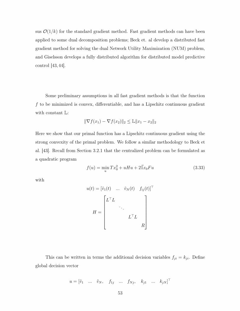
𝑓(𝑢) = min𝑢
𝑇𝑥20 + 𝑢𝐻𝑢+ 2⃗1𝑥0𝐹𝑢 (3.33)
with
𝑢(𝑡) = [𝑣1(𝑡) ... 𝑣𝑁(𝑡) 𝑓𝑖𝑗(𝑡)]⊤
𝐻 =
⎡⎢⎢⎢⎢⎢⎢⎣𝐿⊤𝐿
. . .
𝐿⊤𝐿
𝑅
⎤⎥⎥⎥⎥⎥⎥⎦
This can be written in terms the additional decision variables 𝑓𝑗𝑖 = 𝑘𝑗𝑖. Define
global decision vector
𝑢 = [𝑣1 ... 𝑣𝑁 , 𝑓1𝑗 ... 𝑓𝑁𝑗, 𝑘𝑗1 ... 𝑘𝑗𝑁 ]⊤
53

𝐻 =
⎡⎢⎢⎢⎢⎢⎢⎢⎢⎢⎣
𝐿⊤𝐿. . .
𝐿⊤𝐿
12𝑅
12𝑅
⎤⎥⎥⎥⎥⎥⎥⎥⎥⎥⎦The constraints that we are forming the Lagrangian with are 𝑘𝑗𝑖(𝑡) = 𝑓𝑗𝑖(𝑡) for all
𝑗 ∈ 𝐼(𝑖). To write this in compact form, define
𝐶 =
⎡⎣0−𝐼 𝐼
⎤⎦where 𝐼 are identity matrices with dimensions (𝑚x𝑇 ). Then the equality constraint
𝑘𝑗𝑖(𝑡) = 𝑓𝑗𝑖(𝑡) can be equivalently written as
𝐶𝑢 = 0
We can now write the corresponding Lagrangian dual function as
𝑔(𝜆) = min𝑢
𝑓(𝑢) + 𝜆⊤(𝐶𝑢)
The conjugate 𝑓 * of a function 𝑓 is given by:
𝑓 *(𝑦) = sup𝑢∈𝑑𝑜𝑚(𝑓)
(𝑦⊤𝑢− 𝑓(𝑢))
Notice that the Lagrangian dual 𝑔(𝜆) is equal to
𝑔(𝜆) = −max𝑢
(−𝐶𝜆⊤𝑢− 𝑓(𝑢))
= −𝑓 *(−𝐶𝜆)
Therefore, 𝑔(𝜆) is Lipschitz continuous by an equivalence between strong convexity
in the primal function and properties of its conjugate, proposed in [45], which states
54
that for a proper, lower semi-continuous, convex function 𝑓 : R𝑛 → R and a value 𝜎
the following two properties are equivalent:
(a) 𝑓 * is strongly convex with constant 𝜎
(b) f is differentiable and ∇𝑓 is Lipschitz continuous with constant 1/𝜎
We can use this to find a Lipschitz constant for 𝑔(𝜆). Beck et al. shows that under
these conditions the function 𝑔 has a Lipschitz continuous gradient with constant
‖𝐶‖22/𝜆𝑚𝑖𝑛(𝐻), and that the primal problem converges from 𝑢 → 𝑢* at a rate of
𝒪(1/𝑘) [43]. Gisselson et. al shows that for a strongly convex cost function, the
tightest lower bound on the Lipschitz constant is L ⪰ 𝐶𝐻−1𝐶⊤. Thus we can im-
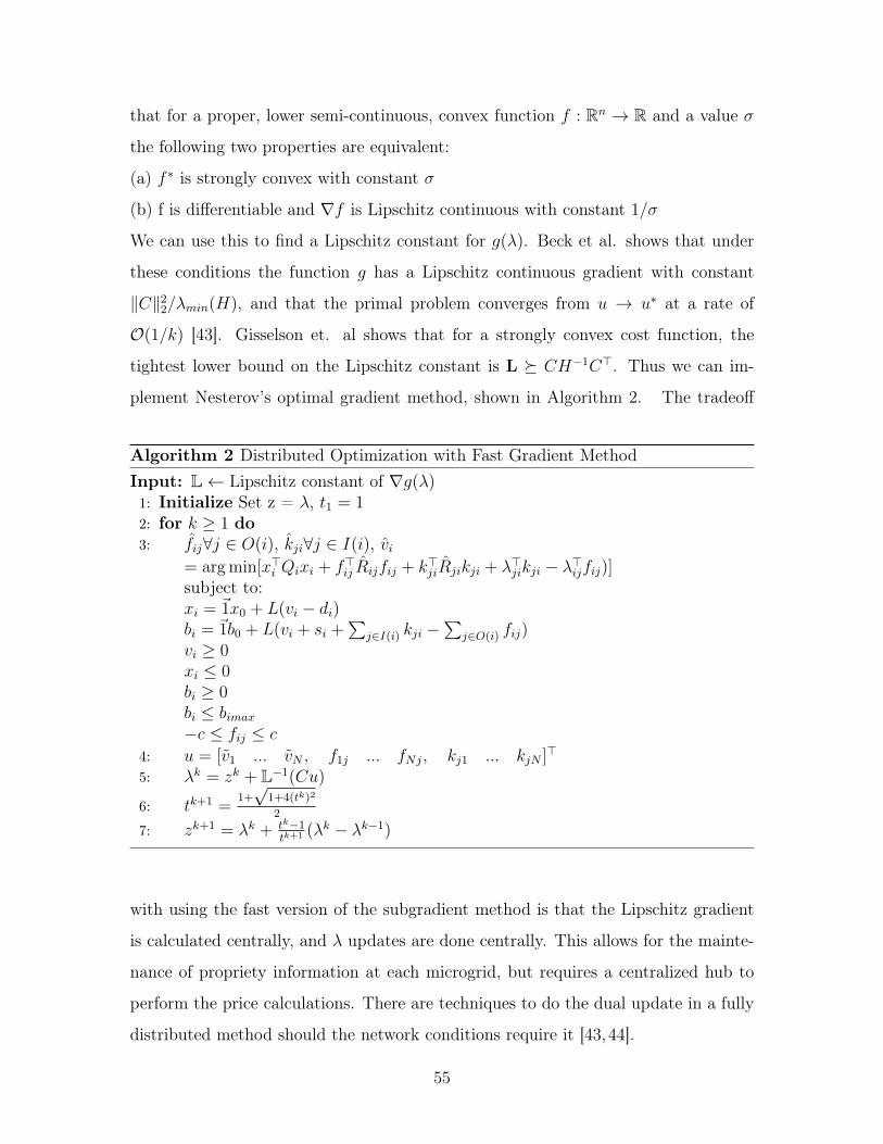
plement Nesterov’s optimal gradient method, shown in Algorithm 2. The tradeoff
Algorithm 2 Distributed Optimization with Fast Gradient MethodInput: L← Lipschitz constant of ∇𝑔(𝜆)1: Initialize Set z = 𝜆, 𝑡1 = 12: for 𝑘 ≥ 1 do3: 𝑓𝑖𝑗∀𝑗 ∈ 𝑂(𝑖), 𝑘𝑗𝑖∀𝑗 ∈ 𝐼(𝑖), 𝑣𝑖
= argmin[𝑥⊤𝑖 𝑄𝑖𝑥𝑖 + 𝑓⊤
𝑖𝑗 �̂�𝑖𝑗𝑓𝑖𝑗 + 𝑘⊤𝑗𝑖�̂�𝑗𝑖𝑘𝑗𝑖 + 𝜆⊤
𝑗𝑖𝑘𝑗𝑖 − 𝜆⊤𝑖𝑗𝑓𝑖𝑗)]
subject to:𝑥𝑖 = 1⃗𝑥0 + 𝐿(𝑣𝑖 − 𝑑𝑖)𝑏𝑖 = 1⃗𝑏0 + 𝐿(𝑣𝑖 + 𝑠𝑖 +
∑︀𝑗∈𝐼(𝑖) 𝑘𝑗𝑖 −
∑︀𝑗∈𝑂(𝑖) 𝑓𝑖𝑗)
𝑣𝑖 ≥ 0𝑥𝑖 ≤ 0𝑏𝑖 ≥ 0𝑏𝑖 ≤ 𝑏𝑖𝑚𝑎𝑥
−𝑐 ≤ 𝑓𝑖𝑗 ≤ 𝑐
4: 𝑢 = [𝑣1 ... 𝑣𝑁 , 𝑓1𝑗 ... 𝑓𝑁𝑗, 𝑘𝑗1 ... 𝑘𝑗𝑁 ]⊤
5: 𝜆𝑘 = 𝑧𝑘 + L−1(𝐶𝑢)
6: 𝑡𝑘+1 =1+√
1+4(𝑡𝑘)2
2
7: 𝑧𝑘+1 = 𝜆𝑘 + 𝑡𝑘−1𝑡𝑘+1 (𝜆
𝑘 − 𝜆𝑘−1)
with using the fast version of the subgradient method is that the Lipschitz gradient
is calculated centrally, and 𝜆 updates are done centrally. This allows for the mainte-
nance of propriety information at each microgrid, but requires a centralized hub to
perform the price calculations. There are techniques to do the dual update in a fully
distributed method should the network conditions require it [43,44].
55

3.5 Dual Decomposition Example
Figure 3-2: Example Micgrogrid Network
Here an example is provided to show the output of the subgradient method.
The method is applied to a five node graph that is connected by six links (see Figure
3-2). The optimization was done over twelve time steps. Supply and demand were
generated randomly for each time point at each node from a uniform distribution
between zero and 1. All initial values were set to zero. In this example we used
constant step size 𝛼 = .01 and terminated the program when the subgradient 𝑠𝑗𝑖 <
.001 for all links. Using a subgradient method, convergence took 19,250 iterations
versus 431 using the fast gradient method.
56
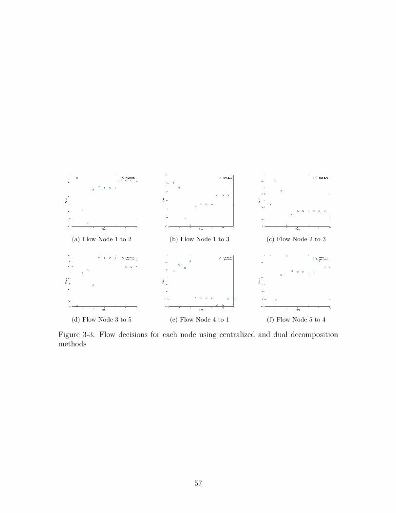
(a) Flow Node 1 to 2 (b) Flow Node 1 to 3 (c) Flow Node 2 to 3
(d) Flow Node 3 to 5 (e) Flow Node 4 to 1 (f) Flow Node 5 to 4
Figure 3-3: Flow decisions for each node using centralized and dual decompositionmethods
57

58

Chapter 4
Dual Decomposition of the LQR
Problem Under Network Flow
Constraints
As discussed in Chapter 2, the constraints on the model explored in Chapters 2 and
3 destroy the structure of the LQR problem. In this chapter we focus on a more
general class of problems. We study a network comprised of local LQR problems
whose decisions are subject to network flow constraints. We use dual decomposition
of the network flow constraints to develop a fully distributed solution that relies on
message passing between nearest neighbor nodes. We then develop a model predictive
control algorithm to compute an approximate distributed policy using only local state
information under uncertain disturbances.
Various techniques for decomposition and coordination for dynamic systems have
been explored in the literature. Cohen develops a generalized iterative algorithm for
the decentralization of dynamic optimal control problems, extending upon Takahara’s
algorithm [46]. Martensson et al. provide a distributed solution for local linear
feedback controller using an iterative gradient method [47]. The method of dual
decomposition has also been used extensively to coordinate dynamic systems coupled
by state and input constraints using model predictive control [44, 48,49].
In this chapter, we apply a dual decomposition technique to a specific case of
59

the decentralized linear quadratic regulator. The work in this chapter extends two
very well known theories. The first is the well known Linear Quadratic Regulator
problem, as described in Chapter 2. Recall that for quadratic cost function 𝐽(𝑥𝑡, 𝑢𝑡)
𝐽(𝑥𝑡, 𝑢𝑡) = min𝑢
E𝑤𝑡{𝑥(𝑇 )⊤𝑄𝑥(𝑇 ) +𝑇−1∑︁𝑡=0
𝑥⊤(𝑡)𝑄𝑥(𝑡) + 𝑢⊤(𝑡)𝑅𝑢(𝑡)}
subject to: 𝑥(𝑡+ 1) = 𝐴𝑥(𝑡) +𝐵𝑢(𝑡) + 𝑤(𝑡)
the optimal solution is given by
𝜇𝑡(𝑥𝑡) = 𝐿𝑡𝑥𝑡
where 𝐿𝑡 is determined by solving the discrete time Ricatti equation
𝐿𝑡 = −(𝐵⊤𝐾𝑡+1𝐵 +𝑅)−1𝐵⊤𝐾𝑡+1𝐴
with 𝐾 defined as
𝐾𝑡 = 𝑄+ 𝐴⊤𝐾𝑡+1𝐴− 𝐴⊤𝐾𝑡+1𝐵(𝑅 +𝐵⊤𝐾𝑡+1𝐵)−1𝐵⊤𝐾𝑡+1𝐴
Rantzer shows that dual decomposition can be applied to decompose dynamic feed-
back systems with separable quadratic costs whose states are coupled through matrix
𝐴. However, the optimal policy still depends on full information of all states 𝑥 [50].
The second theory we draw upon is the dual decomposition of the single net-
work commodity flow problem. In the single commodity network flow problem, the
goal is to choose the optimal flow across some network 𝐺 = (𝑁,𝐸) subject to flow
conservation constraints. The single network commodity flow problem can be sum-
marized as follows: Define 𝑓𝑗 as the flow on arc 𝑗, where 𝑓𝑗 > 0 implies flow is in the
direction of the link. Then the network flow conservation requirement can be written
as 𝐶𝑓 +𝑑 = 0 where 𝐶 is the incidence matrix of graph G. Given some separable cost
function 𝜑(𝑓) =∑︀𝑛
𝑗=1 𝜑𝑗(𝑓𝑗), with 𝜑𝑗 : R→ R being the strictly convex cost function
60

for arc 𝑗, the Lagrangian dual function can be formulated with no duality gap. Solv-
ing the network flow optimization via the dual results in the optimal solution being
given as a function of the optimal potential difference across each link 𝑗, where the
potential refers to the difference between the dual variables of the end node and start
node of link 𝑗 [51].
There are some nice features of both the unconstrained LQR problem and dual
decomposition of the network flow problem. First, the optimal solution to the LQR
problem can be calculated ahead of time as a function of current state 𝑥𝑖, making it
a very useful solution for handling uncertainty online. The advantage of the network
flow problem is that it elegantly decomposes to have strong duality while only relying
on nearest neighbor communication. In this section, the theories underlying these
two problems are leveraged to find a distributed solution to a set of networked LQR
problems, where the local states at each node depend on decisions that are subject
to network flow constraints.
4.1 The Model
We are given some network represented by a connected, directed graph 𝐺 = (𝑁,𝐸)
with known topology of 𝑛 nodes and 𝑚 edges. Each node 𝑛 can have multiple local
state variables 𝑥𝑖 ∈ R𝑧𝑖 . At each time point, nodes must choose the amount of
commodity 𝑑𝑖 to withdraw from or add to the network. State 𝑥𝑖 represents a buffer,
allowing flexibility in the amount of resource 𝑑𝑖 to supply or demand from the network
at each time. The cost function is quadratic in local states 𝑥𝑖(𝑡) as well as in flow
decisions 𝑢 = [𝑓𝑖𝑗]⊤ for all (𝑖, 𝑗) ∈ 𝐸. Define 𝑥 = [𝑥𝑖]
⊤ for all 𝑖 ∈ 𝑁 . Then the cost
function is given by
min𝑢
E[𝑥(𝑇 )⊤𝑄𝑥(𝑇 ) +𝑇−1∑︁𝑡=1
𝑥(𝑡)⊤𝑄𝑥(𝑡) + 𝑢(𝑡)⊤𝑅𝑢(𝑡)] (4.1)
61

subject to:
𝑥𝑖(𝑡+ 1) = 𝐴𝑖𝑥𝑖(𝑡) + 1⃗𝑑𝑖 + 𝑤𝑖(𝑡) ∀𝑖 (4.2)∑︁𝑗∈𝐼(𝑖)
𝑓𝑗𝑖(𝑡)−∑︁
𝑗∈𝑂(𝑖)
𝑓𝑖𝑗(𝑡) = 𝑑𝑖 ∀𝑖 (4.3)
It is possible to combine the network flow constraint in Equation 4.3 into the dynamics
Equation 4.2:
𝑥𝑖(𝑡+ 1) = 𝐴𝑖𝑥𝑖(𝑡) + 1⃗∑︁𝑗∈𝐼(𝑖)
𝑓𝑗𝑖(𝑡)− 1⃗∑︁
𝑗∈𝑂(𝑖)
𝑓𝑖𝑗(𝑡) + 𝑤𝑖(𝑡) ∀𝑖
Then the system wide dynamics can be written in terms of 𝑥 and 𝑢 as
𝑥(𝑡+ 1) = 𝐴𝑥(𝑡) + �̃�𝑢(𝑡) + 𝑤(𝑡)
where �̃� is given by the incidence matrix of the network
�̃�𝑖𝑗 =
⎧⎪⎪⎪⎪⎪⎨⎪⎪⎪⎪⎪⎩−1, if i is the start node of the jth arc
1, if i is the end node of the jth arc
0, otherwise
(4.4)
with row 𝑖 repeated 𝑧𝑖 times for each local state 𝑥𝑖. Assume that matrices 𝑄 and 𝐴
are block diagonal with 𝑛 blocks 𝑄𝑖 and 𝐴𝑖 of size [𝑧𝑖 × 𝑧𝑖], and that 𝑄 is positive
semidefinite and each block 𝐴𝑖 is stable. Also assume 𝑅 is a positive definite diagonal
matrix. Just as in Chapter 2, the flow decisions are coupled across nodes. In order
to decouple the problem we apply dual decomposition. Once again, define variables
62

𝑘𝑗𝑖 = 𝑓𝑗𝑖; then the problem can be formulated as
min𝑢
E𝑤𝑡 [∑︁𝑖∈𝑁
𝑥𝑖(𝑇 )⊤𝑄𝑥𝑖(𝑇 ) +
𝑇−1∑︁𝑡=0
(𝑥⊤𝑖 (𝑡)𝑄𝑥𝑖(𝑡) + 𝑢(𝑡)⊤�̂�𝑢(𝑡))]
subject to: 𝑥𝑖(𝑡+ 1) = 𝐴𝑖𝑥𝑖(𝑡) +∑︁𝑗∈𝐼(𝑖)
𝑘𝑗𝑖(𝑡)−∑︁
𝑗∈𝑂(𝑖)
𝑓𝑖𝑗(𝑡) + 𝑤𝑖(𝑡) ∀𝑖 ∈ 𝑁
𝑘𝑗𝑖(𝑡) = 𝑓𝑗𝑖(𝑡) ∀𝑗 ∈ 𝐼(𝑖)
The coupling in our decisions is now confined to the last constraint 𝑘𝑗𝑖(𝑡) = 𝑓𝑗𝑖(𝑡).
To eliminate the coupling constraint we formulate the Lagrangian dual problem:
L(𝜆𝑖𝑗, 𝑢𝑖, 𝑓𝑖𝑗, 𝑘𝑖𝑗) = max𝜆
min𝑢𝑖,𝑓𝑗𝑖,𝑘𝑗𝑖
E𝑤𝑡{∑︁𝑖∈𝑁
𝑥𝑖(𝑇 )⊤𝑄𝑖𝑥𝑖(𝑇 )
+𝑇−1∑︁𝑡=0
(𝑥⊤𝑖 (𝑡)𝑄𝑖𝑥𝑖(𝑡) + 𝑢(𝑡)⊤�̂�𝑢(𝑡)) + 𝜆𝑗𝑖(𝑡)
⊤(𝑘𝑗𝑖(𝑡)− 𝑓𝑗𝑖(𝑡))}
Using results from Propositions 1 and 2, and define 𝑢𝑖(𝑡) = [𝑓𝑖𝑗(𝑡) 𝑘𝑗𝑖]⊤, then we
know that we can write the Lagrangian as
L(·) =max𝜆
min𝑢𝑖,𝑓𝑖𝑗∀𝑗∈𝑂(𝑖),𝑘𝑗𝑖∀𝑗∈𝐼(𝑖)
E𝑤𝑡 [∑︁𝑖∈𝑁
𝑥𝑖(𝑇 )⊤𝑄𝑖𝑥𝑖(𝑇 ) (4.5)
+𝑇−1∑︁𝑡=0
(𝑥⊤𝑖 (𝑡)𝑄𝑖𝑥𝑖(𝑡) + 𝑢⊤
𝑖 (𝑡)�̂�𝑖𝑢𝑖(𝑡)) + 𝜆𝑗𝑖(𝑡)⊤𝑘𝑗𝑖(𝑡)− 𝜆𝑖𝑗(𝑡)𝑓𝑖𝑗(𝑡))]
where �̂� is again defined as 12𝑅. Define vector
�̃�𝑖(𝑡) = [𝜆𝑗𝑖(𝑡) − 𝜆𝑖𝑗(𝑡)]⊤
Now we can write the optimization at each node only in terms of 𝑢𝑖. Stage cost
at each node 𝑖 can be written as
𝑙𝑖(𝑥𝑖(𝑡)) = 𝑥𝑖(𝑡)⊤𝑄𝑖𝑥𝑖(𝑡) + 𝑢𝑖(𝑡)
⊤𝑅𝑖𝑢𝑖(𝑡) + �̃�𝑖(𝑡)⊤𝑢𝑖(𝑡) (4.6)
63
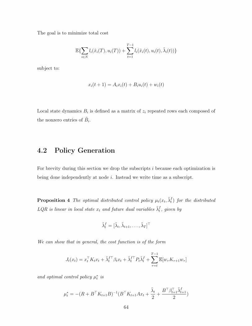
The goal is to minimize total cost
E{∑︁𝑖∈𝑁
𝑙𝑖(�̃�𝑖(𝑇 ), 𝑢𝑖(𝑇 )) +𝑇−1∑︁𝑡=1
𝑙𝑖(�̃�𝑖(𝑡), 𝑢𝑖(𝑡), �̃�𝑖(𝑡))}
subject to:
𝑥𝑖(𝑡+ 1) = 𝐴𝑖𝑥𝑖(𝑡) +𝐵𝑖𝑢𝑖(𝑡) + 𝑤𝑖(𝑡)
Local state dynamics 𝐵𝑖 is defined as a matrix of 𝑧𝑖 repeated rows each composed of
the nonzero entries of �̃�𝑖.
4.2 Policy Generation
For brevity during this section we drop the subscripts 𝑖 because each optimization is
being done independently at node 𝑖. Instead we write time as a subscript.
Proposition 4 The optimal distributed control policy 𝜇𝑡(𝑥𝑡, �̃�𝑓𝑡 ) for the distributed
LQR is linear in local state 𝑥𝑡 and future dual variables �̃�𝑓𝑡 , given by
�̃�𝑓𝑡 = [�̃�𝑡, �̃�𝑡+1, . . . , �̃�𝑇 ]
⊤
We can show that in general, the cost function is of the form
𝐽𝑡(𝑥𝑡) = 𝑥⊤𝑡 𝐾𝑡𝑥𝑡 + �̃�𝑓⊤
𝑡 𝛽𝑡𝑥𝑡 + �̃�𝑓⊤𝑡 𝑃𝑡�̃�
𝑓𝑡 +
𝑇−1∑︁𝜏=𝑡
E[𝑤𝜏𝐾𝜏+1𝑤𝜏 ]
and optimal control policy 𝜇*𝑡 is
𝜇*𝑡 = −(𝑅 +𝐵⊤𝐾𝑡+1𝐵)−1(𝐵⊤𝐾𝑡+1𝐴𝑥𝑡 +
�̃�𝑡
2+
𝐵⊤𝛽⊤𝑡+1�̃�
𝑓𝑡+1
2)
64

Proof By backwards induction:
𝐽𝑇−1(𝑥𝑇−1) = min𝑢𝑇−1
E[�̃�⊤𝑇−1𝑄�̃�𝑇−1 + 𝑢⊤
𝑇−1𝑅𝑢𝑇−1 + �̃�⊤𝑇−1𝑢𝑇−1+
(𝐴�̃�𝑇−1 +𝐵𝑢𝑇−1 + 𝑤𝑇−1)⊤𝑄(𝐴�̃�𝑇−1 +𝐵𝑢𝑇−1 + 𝑤𝑇−1)] (4.7)
Expanding the above equation, and assuming that the mean of our disturbances are
zero, eliminate cross terms with 𝑤:
𝐽𝑇−1(𝑥𝑇−1) = min𝑢𝑇−1
{�̃�⊤𝑇−1𝑄�̃�𝑇−1 + 𝑢⊤
𝑇−1𝑅𝑢𝑇−1 + �̃�⊤𝑇−1𝑢𝑇−1
+ 𝑢⊤𝑇−1𝐵
⊤𝑄𝐵𝑢𝑇−1 + 2𝑥𝑇−1𝐴⊤𝑄𝐵𝑢𝑇−1 + 𝑥⊤
𝑇−1𝐴⊤𝑄𝐴𝑥𝑇−1
+ E[𝑤𝑇−1𝑄𝑤𝑇−1]}
Differentiating with respect to 𝑢𝑇−1 and setting the derivative equal to zero, we find
optimal value of 𝑢𝑇−1:
𝑢*𝑇−1 = −(𝑅 +𝐵⊤𝑄𝐵)−1(𝐵⊤𝑄𝐴𝑥𝑇−1 +
�̃�𝑇−1
2)
Plugging this back in for 𝐽𝑇−1:
𝐽𝑇−1(𝑥𝑇−1) =𝑥⊤𝑇−1𝐾𝑇−1𝑥𝑇−1
− �̃�⊤𝑇−1(𝑅 +𝐵⊤𝑄𝐵)−1𝐵⊤𝑄𝐴𝑥𝑇−1
−�̃�⊤𝑇−1
2(𝑅 +𝐵⊤𝑄𝐵)−1 �̃�𝑇−1
2+ E[𝑤𝑇−1𝑄𝑤𝑇−1]
and define vector 𝛽𝑇−1 = −(𝑅 +𝐵⊤𝑄𝐵)−1𝐵⊤𝑄𝐴. Then
𝐽𝑇−1(𝑥𝑇−1) =𝑥⊤𝑇−1𝐾𝑇−1𝑥𝑇−1 + �̃�⊤
𝑇−1𝛽⊤𝑇−1𝑥𝑇−1
−�̃�⊤𝑇−1
2(𝑅 +𝐵⊤𝑄𝐵)−1 �̃�𝑇−1
2+ E[𝑤𝑇−1𝑄𝑤𝑇−1]
65
Continuing induction, we have
𝐽𝑇−2(𝑥𝑇−2) = min𝑢𝑇−1
E[𝑥⊤𝑇−2𝑄𝑥𝑇−2 + 𝑢⊤
𝑇−2𝑅𝑢𝑇−2 + �̃�𝑇−2 · 𝑢𝑇−2
+ (𝐴�̃�𝑇−2 +𝐵𝑇−2𝑢𝑇−2 + 𝑤𝑇−2)⊤𝐾𝑇−1(𝐴𝑥𝑇−2 +𝐵𝑇−2𝑢𝑇−2 + 𝑤𝑇−2)
⊤
+ �̃�⊤𝑇−1𝛽𝑇−1(𝐴𝑥𝑇−2 +𝐵𝑇−2𝑢𝑇−2 + 𝑤𝑇−2)
⊤
−�̃�⊤𝑇−1
2(𝑅 +𝐵⊤𝑄𝐵)−1 �̃�𝑇−1
2+ 𝑤𝑇−1𝑄𝑤𝑇−1] (4.8)
Taking the derivative over 𝑢𝑇−2 we find
𝑢*𝑇−2 = −(𝑅 +𝐵⊤𝐾𝑇−1𝐵)−1(𝐵⊤𝐾𝑇−1𝐴�̃�𝑇−2 +
�̃�𝑇−2
2+
𝐵⊤𝛽⊤𝑇−1�̃�𝑇−1
2)
Define
𝛽𝑇−2 =
⎡⎣ −(𝑅 +𝐵⊤𝐾𝑇−1𝐵)−1𝐵⊤𝐾𝑇−1𝐴
−𝛽𝑇−1(𝐵(𝑅 +𝐵⊤𝐾𝑇−1𝐵)−1𝐵⊤𝐾𝑇−1 − 𝐼)𝐴
⎤⎦and [(𝑇 − 𝑡)× 1] vector of future prices �̃�𝑓
𝑡 ⊂ �̃�
�̃�𝑓𝑡 = [�̃�𝑡, �̃�𝑡+1, . . . , �̃�𝑇 ]
⊤
Then the value function at 𝑇 − 2 can be written
𝐽𝑇−2(𝑥𝑇−2) = 𝑥⊤𝑇−2𝐾𝑇−2𝑥𝑇−2 + �̃�𝑓⊤
𝑇−2𝛽𝑇−2𝑥𝑇−2
+�̃�𝑓⊤𝑇−2𝑃𝑇−2𝜆
𝑓𝑇−2 +
𝑇−1∑︁𝜏=𝑇−2
E[𝑤𝜏𝐾𝜏+1𝑤𝜏 ]
For arbitrary time 𝑡:
𝐽𝑡(𝑥𝑡) = 𝑥⊤𝑡 𝐾𝑡𝑥𝑡 + �̃�𝑓⊤
𝑡 𝛽𝑡𝑥𝑡 + �̃�𝑓⊤𝑡 𝑃𝑡�̃�
𝑓𝑡 +
𝑇−1∑︁𝜏=𝑡
E[𝑤𝜏𝐾𝜏+1𝑤𝜏 ]
66

Then for 𝐽𝑡−1:
𝐽𝑡−1(𝑥𝑡−1) =min𝑢𝑡−1
E[𝑥⊤𝑡−1𝑄𝑥𝑡−1 + 𝑢⊤
𝑡−1𝑅𝑢𝑡−1 + �̃�𝑇𝑡−1𝑢𝑡−1
+ (𝐴𝑥𝑡−1 +𝐵𝑢𝑡−1 + 𝑤𝑡−1)⊤𝐾𝑡(𝐴𝑥𝑡−1 +𝐵𝑢𝑡−1 + 𝑤𝑡−1)
+ �̃�𝑓⊤𝑡 𝛽𝑡(𝐴𝑥𝑡−1 +𝐵𝑢𝑡−1 + 𝑤𝑡−1)]
+ �̃�𝑓⊤𝑡 𝑃𝑡�̃�
𝑓𝑡 +
𝑇−1∑︁𝜏=𝑡
E[𝑤𝜏𝐾𝜏+1𝑤𝜏 ]
Taking the derivative with respect to 𝑢𝑡−1 and setting equal to zero, we find
𝑢*𝑡−1 = −(𝑅 +𝐵⊤𝐾𝑡𝐵)−1(𝐵⊤𝐾𝑡𝐴𝑥𝑡−1 + 1/2(�̃�𝑡−1 +𝐵⊤𝛽⊤
𝑡 �̃�𝑓𝑡 ))
Plugging back into the value function with
𝛽𝑡−1 =
⎡⎣ −(𝑅 +𝐵⊤𝐾𝑡𝐵)−1𝐵⊤𝐾𝑡𝐴
−𝛽𝑡(𝐵(𝑅 +𝐵⊤𝐾𝑡𝐵)−1𝐵⊤𝐾𝑡 − 𝐼)𝐴
⎤⎦and
�̃�𝑓𝑡−1 = [�̃�𝑡−1, �̃�𝑡, . . . , �̃�𝑇 ]
⊤
we can re-write the cost to go as
𝐽𝑡−1(𝑥𝑡−1) = 𝑥⊤𝑡−1𝐾𝑡−1𝑥𝑡−1 + �̃�𝑓⊤
𝑡−1𝛽𝑡−1𝑥𝑡−1
+ �̃�𝑓⊤𝑡−1𝑃𝑡−1�̃�
𝑓𝑡−1 +
𝑇−1∑︁𝜏=𝑡−1
E[𝑤⊤𝜏 𝐾𝜏+1𝑤𝜏 ]
which is the same form as we started with.
4.3 Price update and Receding Horizon Control
The optimal distributed decision depends on the values of current and future dual
variables. For every iteration 𝑘, we approximate the values of dual variables �̃� by
performing a forward propagation of our system under policy 𝜇𝑘(�̃�) and the expected
67

value of disturbances 𝑤. This is shown in Algorithm 3. To update the dual vector
�̃�𝑖(𝑡), a gradient method can be implemented. Recall from equation (4.6) that the
gradient over the nodal dual variable 𝜆𝑗𝑖 is given by 𝑠𝑗𝑖 = 𝑘𝑗𝑖 − 𝑓𝑗𝑖. This update
must happen at every node, relying on the communication from neighbors of their
flow decisions 𝑓𝑗𝑖:
𝜆𝑘+1𝑗𝑖 = 𝜆𝑘
𝑗𝑖 − 𝛼𝑘𝑠𝑘𝑗𝑖
After calculating 𝜆𝑗𝑖(𝑡) at each node for all 𝑡, �̃�𝑖(𝑡) can be formed by communicating
values of 𝜆’s between the nodes’ neighbors. Convergence of the algorithm follows
from the same subgradient results shown in Section 3.3.
For deterministic problems, the forward propagation of the system is exact, and
the policy provides the exact optimal solution. Under uncertainty, the the estimation
of the future price vector is an approximation given predicted disturbance E[𝑤(𝑡)].
Because the future prices are estimated using current local state 𝑥𝑖, the algorithm is
implemented as a receding horizon control algorithm. This means that the policy is
applied to the first decision, then the calculation is done again once the disturbance at
that time point has been realized. The advantage of the algorithm over conventional
model predictive control solutions using dual decomposition is that the minimization
problem has been calculated offline, so no minimization has to take place at every
iteration.
At every stage, there is error accruing for two reasons. The first is the error
in 𝜆𝑖 given our decision to terminate the algorithm when max(𝑠𝑗𝑖) < 𝜖. The second
is during the forward propagation of the system dynamics. In order to generate the
future price estimates, the future states 𝑥𝑖 must also be estimated by propagating the
system forward 𝑥𝑖(𝑡 + 1) = 𝐴𝑥𝑖(𝑡) + 𝐵𝑖𝑢𝑖(𝑡) (because E[𝑤𝑖(𝑡)]] = 0). For each time
point 𝑡 any variance in the disturbance 𝑤𝑖 will be multiplied by matrix A. Thus A is
constrained to be a stable matrix.
68

Algorithm 3 Distributed LQR
Input: �̃�𝑖 , �̃�𝑖(1)1: Initialize Set �̃�𝑖 = 0⃗
𝐾𝑖(𝑇 ) = 𝑄,𝛽𝑖(𝑇 − 1) = −(𝑅𝑖 +𝐵⊤
𝑖 𝑄𝐵𝑖)−1𝐵⊤
𝑖 𝑄𝑖𝐴2: for 𝑡 = 𝑇 : −1 : 𝜏 do3: 𝐾𝑖(𝑡− 1) = 𝐴⊤
𝑖 (𝐾𝑖(𝑡)−𝐾𝑖(𝑡)𝐵𝑖(𝐵⊤𝑖 𝐾𝑖(𝑡)𝐵𝑖 +𝑅𝑖)
−1𝐵⊤𝑖 𝐾𝑖(𝑡))𝐴𝑖 +𝑄𝑖
4: for 𝑡 = 𝑇 − 1 : −1 : 𝜏 do
5: 𝛽𝑖(𝑡− 1) =
[︂−(𝑅𝑖 +𝐵⊤
𝑖 𝐾𝑖(𝑡)𝐵𝑖)−1𝐵⊤
𝑖 𝐾𝑖(𝑡)𝐴𝑖
−𝛽𝑖(𝑡)(𝐵𝑖(𝑅𝑖 +𝐵⊤𝑖 𝐾𝑖(𝑡)𝐵𝑖)
−1𝐵⊤𝑖 𝐾𝑖(𝑡)− 𝐼)𝐴𝑖
]︂6: for 𝑘 ≥ 1 do7: for 𝑡 = 𝜏 : 𝑇 − 1 do8: 𝑢𝑖(𝑡) = −(𝑅𝑖 +𝐵⊤
𝑖 𝐾𝑖(𝑡+ 1)𝐵𝑖)−1(𝐵⊤
𝑖 𝐾𝑖(𝑡+ 1)𝐴𝑥𝑖(𝑡)+1/2(�̃�𝑖(𝑡) +𝐵⊤
𝑖 𝛽𝑖(𝑡+ 1)⊤�̃�𝑓𝑖 (𝑡)))
9: 𝑥𝑖(𝑡+ 1) = 𝐴𝑖𝑥𝑖(𝑡) +𝐵𝑖𝑢𝑖(𝑡)
10: 𝑠𝑘𝑗𝑖 = 𝑘𝑗𝑖 − 𝑓𝑗𝑖 where 𝑘𝑗𝑖 ∈ 𝑢𝑖 and 𝑓𝑗𝑖 ∈ 𝑢𝑗∀𝑗 ∈ 𝐼(𝑖)
11: 𝜆𝑘+1𝑗𝑖 = 𝜆𝑘
𝑗𝑖 + 𝛼𝑘𝑠𝑗𝑖12: �̃�𝑖 = [𝜆𝑖𝑗 − 𝜆𝑗𝑖]
⊤
4.4 Performance
At each stage the control policy attempts to minimize cost in spite of disturbances.
To be optimal, the decision of how much of the resource to add or remove from each
buffer requires information about all buffer state 𝑥. In order to assess the performance
of the algorithm, we can compare the decisions generated from Algorithm 3 to the
optimal decisions made using full information for all states 𝑥𝑡, given by the LQR
solution: 𝜇𝑡(𝑥𝑡) = 𝐿𝑡𝑥𝑡. Here we present an example of the distributed algorithm in
comparison to the centralized optimal solution.
The network that is optimized over is shown in Figure 4-1. In the example, there
are four nodes and four links. 𝑄𝑖 and 𝑅𝑖 are the identity matrices. Incidence matrix
for the graph is given by
�̃� =
⎡⎢⎢⎢⎢⎢⎢⎣−1 0 0 1
1 −1 1 0
0 0 −1 0
0 1 0 −1
⎤⎥⎥⎥⎥⎥⎥⎦69

Figure 4-1: Distributed LQR Network
Each node has two states, and
𝐴𝑖 =
⎡⎣.25 .30
.40 .32
⎤⎦Therefore each matrix 𝐵𝑖 is as follows:
𝐵1 =
⎡⎣−1 1
−1 1
⎤⎦ , 𝐵2 =
⎡⎣1 −1 1
1 −1 1
⎤⎦ , 𝐵3 =
⎡⎣−1−1
⎤⎦ , 𝐵4 =
⎡⎣1 −11 −1
⎤⎦Initial states 𝑥𝑜 and offsets 𝑤𝑖(𝑡) at each node are generated from a uniform distri-
bution between [−.5, .5]. Results comparing the distributed and centralized solutions
are compared in Figure 4-2.
70
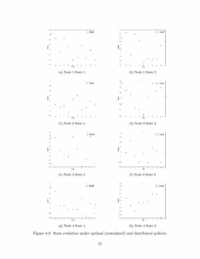
(a) Node 1 State 1 (b) Node 1 State 2
(c) Node 2 State 1 (d) Node 2 State 2
(e) Node 3 State 1 (f) Node 3 State 2
(g) Node 4 State 1 (h) Node 4 State 2
Figure 4-2: State evolution under optimal (centralized) and distributed policies.
71

72

Chapter 5
Conclusions and Future Work
5.1 Overview
As discussed in Chapter 1, electricity access is a global issue that India is particularly
affected by, with an estimated 240 million people without access. Electrification
through conventional generation and grid extension suffers from many drawbacks.
Extending the central grid to villages that are far from existing power plants is very
costly; extending the grid just 5 to 25 km from the nearest existing lines is not cost
competitive. Furthermore, the central government has made electrification through
renewable sources a priority. This has brought down costs of centralized solar projects
significantly. Unfortunately, on-site generation continues to suffer from a lack of
financing, leading to sporadic implementation at small scales. Any technological
advantage that would provide for lower upfront capital costs would allow for a more
competitive energy landscape in which small microgrid operators may be able to
compete more effectively with subsidized energy prices.
5.2 Value of Interconnection
In Chapter 2, a model was developed that would allow for power to be shared across
distinct, individual microgrids. Costs were associated with unmet, backlogged de-
mand, and the cost of transmission between microgrids. The decisions involve opti-
73
mizing both the local demand schedule as well as the amount of energy to transmit
between nodes over a finite team period. The model is deterministic with some supply
and demand forecast, and can be solved centrally as a quadratic program.
Using this model and supply and demand data gathered in India, we showed
that storage capacity could be removed from some microgrids without significantly
altering the overall reliability of the microgrids. Simulations were done to emulate a
25 microgrid network being powered by a 250W solar panel. During months when
there was only critical demand on the system, up to %60 of the storage could be
removed from the network with only a 2% decrease in overall reliability. Over the
whole year, %40 percent of storage could be removed with just a 3% decrease in
reliability. However, there are tradeoffs to removing local storage. These reliability
estimates depend on the cost of transmission relative to the cost of serving unmet
demand, which is directly related to the distance between the microgrids. If storage
is too far from the microgrid it needs to serve, costs of transmission could outweigh
cost of serving demand. In Section 2.3, supply side uncertainty was introduced. We
found that the deterministic model outperforms a system without interconnection
even with supply side variability.
5.3 Decomposability of the Model
Chapter 2 proposed a centralized control system for microgrid interconnection. Often
this may be infeasible in practice, because of limitations in centralized resources and
communication structures, and prioritization in retaining proprietary data. In Chap-
ter 3, the model is decomposed to allow for local autonomy and decision making of
microgrids. We showed that using a dual decomposition technique, we can separate
the optimization so that the microgrids can maintain proprietary supply and demand
forecasts and compute scheduling optimizations locally. The outputs of these local
optimizations are used to update price variables throughout the network, until an
optimal global solution is reached. We show that there is no duality gap between
the distributed solution and the centralized solution, and that only local communi-
74

cation between nearest neighbors is required to facilitate the price variable updates.
This means that interconnection could be implemented in a completely decentralized
fashion.
5.4 Extension to the Distributed LQR
In Chapter 4, the ideas that were generated in formulating the interconnection model
are extended to a more general setting. We focused on a specific class of problems
in which a quadratic cost function is subject to linear dynamics whose decisions de-
pend on network flow constraints. There are many general methods for decomposing
dynamic systems in order to apply local optimization. For this problem, we applied
dual decomposition to the network flow conservation constraints that coupled the
systems. Both the LQR problem and the dual decomposition of network flow con-
straints have elegant solutions. By combining these two bodies of work, we generated
an approximately optimal, fully distributed policy for each state only in terms of local
state variables 𝑥𝑖(𝑡) and price variables �̃�, which only involves message passing be-
tween nearest neighbors. The algorithm presented in Algorithm 3 updates the policy
𝜇𝑖(𝑥𝑖(𝑡)) given some estimates of future price vectors �̃�𝑓𝑖 . The algorithm relies on
approximations depending on current states 𝑥𝑖(𝑡) and is run as a receding horizon
control problem.
5.5 Future Work
Going forward, it would be useful to simulate the model under a larger variety of
simulation parameters. It would be interesting to assess sensitivity and performance
under a variety of conditions. For example, simulating under homogeneous supply
and demand gives a conservative estimate of the value of interconnection; in circum-
stances with more variable supply and demand between nodes interconnection could
provide additional value. A full Monte-Carlo simulation could be generated in order
to find the affects under a variety of different active constraint circumstances. For
75

implementation, parameter choices would have to be made based on the specific net-
work and context, but having a knowledge of sensitivity to different parameters would
assist in the decision making process. Furthermore, if implementation ever happened,
it would be interesting to see feedback on the model itself. There may be practical
conditions that would change the way that the model should be designed for use in
the field.
In general, there are interesting questions that could tackled with the knowledge
that microgrid interconnection potentially has value to offset storage capacity needs.
In Section 2.3, we discussed the impact that storage siting has on microgrids with
similar supply and demand profiles. A potential research question would be to thor-
oughly explore the storage placement question in a more general sense. It would also
be interesting to explore network effects in greater detail. For example, although the
model incorporates congestion constraints, they were often not active at the supply
and demand scale that we are optimizing for. However, it would be important to
assess the effects of congestion on more general microgrid networks, and how they
might impact the fragility of the system.
In the future, uncertainty should be addressed directly in the model. We showed
the the deterministic model is still an improvement over no interconnection, even with
supply side variability. However, this could be made optimal by including variability
in the policy making process. It is possible that the algorithm developed in Chapter
4 could be modified and extended to include constraints. This could possibly be
done by another level of dual decomposition. Finally, Algorithm 3 could be modified
to include decision variables that are not only flow decisions. This would involve
including all decisions in variable 𝑢𝑖, corresponding to adding zero terms into price
vector �̃�𝑖. This would generalize the types of optimizations covered by this Algorithm
beyond problems that only depend on total inflow at node 𝑖.
76

5.6 Final Remarks
This work assessed the value of connecting independent, solar powered microgrids in
India into a larger network. The results show that there is a potential to gain value
by interconnecting microgrids in India, and that having storage at every microgrid
may not be the best use of expensive resources. Instead, connections between micro-
grids allow the storage capacity to be shared while capitalizing on slight variations
between the supply and demand at local microgrids. Given the relatively low cost of
implementing additional short distance transmission versus providing storage capac-
ity, microgrid interconnection has the potential to lower costs of providing energy to
those who reside in off-grid areas in India.
77

78
Bibliography
[1] I. E. Agency, “World energy outlook 2015 executive summary,” Tech. Rep., 2015.
[2] ——, “World energy outlook 2014,” Tech. Rep., 2014. [Online]. Available:
/content/book/weo-2014-en
[3] V. Aggarwal, A. Fahey, H. S. Freymiller, S. Li, C. Huang, and S. Moilanen, “Rural
Energy Alternatives in India : Opportunities in Financing and Community
Engagement for Renewable Energy Microgrid Projects,” Tech. Rep., 2014.
[Online]. Available: https://wws.princeton.edu/sites/default/files/content/591f
Rural Energy Alternatives in India.pdf
[4] S. Pargal and K. Mayer, Governance of Indian State power
utilities : an ongoing journey, 2014. [Online]. Available:
http://documents.worldbank.org/curated/en/2014/09/20268779/governance-
indian-state-power-utilities-ongoing-journey
[5] F. of Regulators, “Report on Road Map for Reduction in Cross Subsidy,” no.
April, 2015.
[6] MNRE, “Jawaharlal Nehru National Solar Mission - Towards building Solar In-
dia,” Www.Mnre.Gov.in, p. 15, 2010.
[7] Ernst&Young, “Mapping India’s Renewable Energy growth potential:,” 2013.
[8] A. Sharma, K. Srivastava, and S. K. Kar, “Jawaharlal Nehru national solar
mission in India,” Green Energy and Technology, vol. 201, pp. 47–67, 2015.
79

[9] P. Sreedharan, R. Ghanadan, L. Alagappan, S. Price, A. Olson, and
R. Bharvirkar, “Electricity grid evolution in India A scoping study on the tech-
nical and planning needs to support the National Action Plan,” p. 116, 2011.
[10] MNRE, “Annual Report 2015-2016,” Tech. Rep., 2016. [Online]. Avail-
able: http://mnre.gov.in/file-manager/annual-report/2015-2016/EN/Chapter
1/chapter_1.htm#1
[11] The Climate Group and Goldman Sachs, “The Business Case
for Off-grid Energy in India,” Tech. Rep., 2013. [Online]. Avail-
able: http://www.theclimategroup.org/_assets/files/The-business-case-for-
offgrid-energy-in-India.pdf
[12] A. Gambhir, V. Toro, and M. Ganapathy, “Decentralised Renewable Energy (
DRE ) Microgrids in India,” Prayas Energy Group, Tech. Rep. November, 2012.
[13] J. Urpelainen and S. Yoon, “Energy for sustainable development solar home
systems for rural india : Survey evidence on awareness and willingness to pay
from uttar pradesh,” Energy for Sustainable Development, vol. 24, pp. 70–78,
2015. [Online]. Available: http://dx.doi.org/10.1016/j.esd.2014.10.005
[14] D. E. Olivares, A. Mehrizi-Sani, A. H. Etemadi, C. A. Cañizares, R. Iravani,
M. Kazerani, A. H. Hajimiragha, O. Gomis-Bellmunt, M. Saeedifard, R. Palma-
Behnke, G. A. Jiménez-Estévez, and N. D. Hatziargyriou, “Trends in microgrid
control,” IEEE Transactions on Smart Grid, vol. 5, no. 4, pp. 1905–1919, 2014.
[15] T. L. Vandoorn, J. C. Vásquez, J. De Kooning, J. M. Guerrero, and L. Vande-
velde, “Hierarchical Control and an Overview of the Control and Reserve Man-
agement Strategies,” IEEE Industrial Electronics Magazine, no. december 2013,
pp. 42–55, 2013.
[16] S. Borenstein, M. Jaske, and A. Rosenfeld, “Dynamic Pricing, Advanced
Metering, and Demand Response in Electricity Markets,” 2002. [Online].
Available: http://www.escholarship.org/uc/item/11w8d6m4
80

[17] M. Pipattanasomporn, H. Feroze, and S. Rahman, “Multi-agent systems in
a distributed smart grid: Design and implementation,” in 2009 IEEE/PES
Power Systems Conference and Exposition. IEEE, mar 2009, pp. 1–8. [Online].
Available: http://ieeexplore.ieee.org/articleDetails.jsp?arnumber=4840087
[18] D. Materassi, M. Roozbehani, and M. A. Dahleh, “Equilibrium price distribu-
tions in energy markets with shiftable demand,” in 2012 IEEE 51st IEEE Confer-
ence on Decision and Control (CDC). IEEE, dec 2012, pp. 3183–3188. [Online].
Available: http://ieeexplore.ieee.org/articleDetails.jsp?arnumber=6425845
[19] M. Roozbehani, M. A. Dahleh, and S. K. Mitter, “Volatility of Power
Grids Under Real-Time Pricing,” IEEE Transactions on Power Sys-
tems, vol. 27, no. 4, pp. 1926–1940, nov 2012. [Online]. Available:
http://ieeexplore.ieee.org/articleDetails.jsp?arnumber=6197252
[20] A. Subramanian, M. Garcia, A. Dominguez-Garcia, D. Callaway, K. Poolla,
and P. Varaiya, “Real-time scheduling of deferrable electric loads,” in 2012
American Control Conference (ACC). IEEE, jun 2012, pp. 3643–3650. [Online].
Available: http://ieeexplore.ieee.org/articleDetails.jsp?arnumber=6315670
[21] A. Papavasiliou and S. S. Oren, “Large-Scale Integration of Deferrable
Demand and Renewable Energy Sources,” IEEE Transactions on Power
Systems, vol. 29, no. 1, pp. 489–499, jan 2014. [Online]. Available:
http://ieeexplore.ieee.org/articleDetails.jsp?arnumber=6494362
[22] D. Madjidian, M. Roozbehani, and M. A. Dahleh, “Emulating Batteries with
Deferrable Energy Demand: Fundamental Trade-offs and Scheduling Policies,”
2016. [Online]. Available: http://arxiv.org/abs/1611.03765
[23] A. G. Tsikalakis and N. D. Hatziargyriou, “Centralized Control for
Optimizing Microgrids Operation,” IEEE Transactions on Energy Con-
version, vol. 23, no. 1, pp. 241–248, mar 2008. [Online]. Available:
http://ieeexplore.ieee.org/articleDetails.jsp?arnumber=4454000
81

[24] A. Papavasiliou and S. S. Oren, “Supplying renewable energy to de-
ferrable loads: Algorithms and economic analysis,” in IEEE PES
General Meeting. IEEE, jul 2010, pp. 1–8. [Online]. Available:
http://ieeexplore.ieee.org/articleDetails.jsp?arnumber=5589405
[25] M. Neely, a.S. Tehrani, and a.G. Dimakis, “Efficient Algorithms for Renewable
Energy Allocation to Delay Tolerant Consumers,” Smart Grid Communications
(SmartGridComm), 2010 First IEEE International Conference on, pp. 1–10,
2010.
[26] B. R. Deshmukh, G. Ghatikar, R. Yin, and G. G. Das, “Estimation of Potential
and Value of Demand Response for Industrial and Commercial Consumers in
Delhi,” 2015.
[27] V. Singh, L. Teja, and J. Tiwari, “Direct Current and Alternative Current Based
Solar Micro-Grid in Rural Energy Infrastructure,” J Fundam Renewable Energy
Appl, vol. 6, no. 1, pp. 1–5, 2015.
[28] D. Bertsekas, Dynamic Programming and Optimal Control, 1st ed. Belmont:
Athena Scientific, 2000.
[29] D. Bertsimas and D. B. Brown, “Constrained stochastic LQC: A tractable ap-
proach,” IEEE Transactions on Automatic Control, vol. 52, no. 10, pp. 1826–
1841, 2007.
[30] Z. Zhou, “Stochastic LQ Control with Probabilistic Constraints,”
Ph.D. dissertation, University of Virginia, 2012. [Online]. Available:
http://libra.virginia.edu/catalog/libra-oa:2633
[31] P. O. M. Scokaert and J. B. Rawlings, “Constrained linear quadratic regulation,”
IEEE Transactions on Automatic Control, vol. 43, no. 8, pp. 1163–1169, 1998.
[32] M. Sznaier and M. Damborg, “Suboptimal control of linear systems with state
and control inequality constraints,” 26th IEEE Conference on Decision and
82

Control, 1987., vol. 26, no. December, pp. 761–762, 1987. [Online]. Available:
http://ieeexplore.ieee.org/xpls/abs_all.jsp?arnumber=4049368
[33] A. Bemporad, M. Morari, V. Dua, and E. N. Pistikopoulos, “The explicit linear
quadratic regulator for constrained systems,” Automatica, vol. 38, no. 1, pp.
3–20, 2002.
[34] V. Mehra, “Optimal Sizing of Solar and Battery Assets in Decentralized Micro-
Grids with Demand-Side Management,” Ph.D. dissertation, Massachusetts Insti-
tute of Technology, 2017.
[35] D. Antoniou, A. Tzimas, and S. M. Rowland, “Transition from alternating current
to direct current low voltage distribution networks,” IET Generation, Trans-
mission & Distribution, vol. 9, no. 12, pp. 1391–1401, 2015. [Online]. Available:
http://digital-library.theiet.org/content/journals/10.1049/iet-gtd.2014.0823
[36] S. Boyd and L. Vandenberghe, Convex Optimization. Cambridge University
Press, 2004.
[37] M. Chiang, S. H. Low, A. R. Calderbank, and J. C. Doyle, “Layering as opti-
mization decomposition: A mathematical theory of network architectures,” Pro-
ceedings of the IEEE, vol. 95, no. 1, pp. 255–312, Jan 2007.
[38] S. Boyd and A. Mutapcic, “Notes on subgradient methods,” 2008.
[39] Y. Nesterov, “A method of solving a convex programming problem with conver-
gence rate o (1/k2),” 1983.
[40] ——, “Smooth minimization of non-smooth functions,” Mathematical Pro-
gramming, vol. 103, no. 1, pp. 127–152, 2005. [Online]. Available:
http://dx.doi.org/10.1007/s10107-004-0552-5
[41] A. Beck and M. Teboulle, “A Fast Iterative Shrinkage-Thresholding Algorithm,”
Society for Industrial and Applied Mathematics Journal on Imaging Sciences,
vol. 2, no. 1, pp. 183–202, 2009.
83

[42] P. Tseng, “On accelerated proximal gradient methods for convex-concave opti-
mization,” submitted to SIAM Journal on Optimization, 2008.
[43] A. Beck and A. Nedic, “Optimal Distributed Gradient Methods for Network
Resource Allocation Problems,” pp. 1–20, 2013.
[44] P. Giselsson, Improved dual decomposition for distributed model pre-
dictive control. IFAC, 2014, vol. 19, no. 3. [Online]. Available:
http://dx.doi.org/10.3182/20140824-6-ZA-1003.00294
[45] R. T. Rockafellar and R. J.-B. Wets, Variational analysis., ser. Grundlehren der
mathematischen Wissenschaften: 317. Berlin ; New York : Springer, c1998.,
1998.
[46] G. Cohen, “On an Algorithm of Decentralized Optimal Control,” Journal of
Mathematical Analysis and Applications, no. 59, pp. 242–259, 1977.
[47] K. Mårtensson and A. Rantzer, “Gradient methods for iterative distributed con-
trol synthesis,” Conference on Decision and Control, pp. 1–6, 2009.
[48] B. Biegel, J. Stoustrup, and P. Andersen, “Distributed MPC Via Dual Decom-
position,” in Distributed Model Predictive Control Made Easy, 2004, ch. 11, pp.
179–192.
[49] Y. Wakasa, M. Arakawa, K. Tanaka, and T. Akashi, “Decentralized model
predictive control via dual decomposition,” 2008 47th IEEE Conference on
Decision and Control, vol. 22, no. 10, pp. 381–386, 2008. [Online]. Available:
http://ieeexplore.ieee.org/lpdocs/epic03/wrapper.htm?arnumber=4739012
[50] A. Rantzer, “Dynamic dual decomposition for distributed control,” Proceedings
of the American Control Conference, pp. 884–888, 2009.
[51] S. Boyd, L. Xiao, A. Mutapcic, and J. Mattingley, “Notes on Decomposition
Methods,” pp. 1–36, 2008.
84