rotary elastic actuator - core
TRANSCRIPT

ROTARY ELASTIC ACTUATOR
CHAI MIN-WUI EDDIE(B.Eng(Hons.),Adelaide)
A THESIS SUBMITTED
FOR THE DEGREE OF MASTER OF ENGINEERING
DEPARTMENT OF MECHANICAL ENGINEERING
NATIONAL UNIVERSITY OF SINGAPORE
2004

Acknowlegdements
I would like to thank my supervisor, Assoc. Prof Marcelo H. Ang Jr. for his continual
guidance and support to improve my actuator, and his faith that this actuator will
work.
I would also like to thank those who have helped over the year. I have appreciated
discussions with Dr Lu Tien Fu from Adelaide University and fellow uni-mates Eddie
Choong, Chua Kian Ti and Sosodoro. I won’t have come so far without them!
The lab technicians, Mr. Zhang, Mrs. Ooi, Ms. Tshin and Mdm. Hamidah have
all been very helpful indeed. I could not have done so much without their assistance
with all the paperwork and hard labour.
Thanks to my family and friends who have been there all the while, to give me
support.
ii

Table of Contents
Acknowlegdements ii
Table of Contents iii
Summary vi
List of Tables vii
List of Figures viii
1 Introduction 1
1.1 Background . . . . . . . . . . . . . . . . . . . . . . . . . . . . . . . . 1
1.2 Scope of Investigation . . . . . . . . . . . . . . . . . . . . . . . . . . 4
1.3 Review of Thesis Content . . . . . . . . . . . . . . . . . . . . . . . . 5
2 Related Work 6
2.1 Introduction . . . . . . . . . . . . . . . . . . . . . . . . . . . . . . . . 6
2.2 Interactions between robots and environments . . . . . . . . . . . . . 7
2.2.1 Passive Compliant . . . . . . . . . . . . . . . . . . . . . . . . 7
2.2.2 Active Control . . . . . . . . . . . . . . . . . . . . . . . . . . 8
2.3 Recent Developments in Elastic Actuator . . . . . . . . . . . . . . . . 10
2.3.1 Electro-magnetic (EM) . . . . . . . . . . . . . . . . . . . . . . 11
2.3.2 Hydraulic . . . . . . . . . . . . . . . . . . . . . . . . . . . . . 14
2.3.3 Pneumatic . . . . . . . . . . . . . . . . . . . . . . . . . . . . . 15
2.4 Recent development in position control . . . . . . . . . . . . . . . . . 16
3 Modelling and Control 18
3.1 Introduction . . . . . . . . . . . . . . . . . . . . . . . . . . . . . . . . 18
3.2 Model of Actuator . . . . . . . . . . . . . . . . . . . . . . . . . . . . 18
iii

3.2.1 Rigid Actuator(RA) . . . . . . . . . . . . . . . . . . . . . . . 18
3.2.2 Elastic Actuator(EA) . . . . . . . . . . . . . . . . . . . . . . . 21
3.3 Control . . . . . . . . . . . . . . . . . . . . . . . . . . . . . . . . . . 23
3.3.1 Position Control of Rigid Actuator(RA) . . . . . . . . . . . . 24
3.3.2 Position Control of Rotary Elastic Actuator(REA) . . . . . . 24
3.3.3 Torque Control . . . . . . . . . . . . . . . . . . . . . . . . . . 26
3.3.4 Force Control: Contact Start . . . . . . . . . . . . . . . . . . 27
3.3.5 Force Control: Moving to Contact . . . . . . . . . . . . . . . . 29
4 Actuator Design 33
4.1 Introduction . . . . . . . . . . . . . . . . . . . . . . . . . . . . . . . . 33
4.2 The Power-train System . . . . . . . . . . . . . . . . . . . . . . . . . 35
4.3 Elastic Flywheel Design . . . . . . . . . . . . . . . . . . . . . . . . . 36
4.4 Characteristic of Elastic Flywheel . . . . . . . . . . . . . . . . . . . . 41
4.5 Sensor System . . . . . . . . . . . . . . . . . . . . . . . . . . . . . . . 42
4.5.1 Method of Sensing . . . . . . . . . . . . . . . . . . . . . . . . 42
4.5.2 Choice of Sensors . . . . . . . . . . . . . . . . . . . . . . . . . 43
4.6 Testing of Elastic Flywheel . . . . . . . . . . . . . . . . . . . . . . . . 44
4.7 Experiment Setup . . . . . . . . . . . . . . . . . . . . . . . . . . . . . 47
5 Simulation and Experiment Results 49
5.1 Introduction . . . . . . . . . . . . . . . . . . . . . . . . . . . . . . . . 49
5.2 Calibration . . . . . . . . . . . . . . . . . . . . . . . . . . . . . . . . 49
5.3 Dynamic Identification . . . . . . . . . . . . . . . . . . . . . . . . . . 55
5.3.1 Static Friction . . . . . . . . . . . . . . . . . . . . . . . . . . . 55
5.3.2 Dynamic Friction and Inertia . . . . . . . . . . . . . . . . . . 56
5.4 Position Control . . . . . . . . . . . . . . . . . . . . . . . . . . . . . . 57
5.4.1 Position Control: Step Response . . . . . . . . . . . . . . . . . 57
5.4.2 Position Control: Trajectory Response . . . . . . . . . . . . . 60
5.5 Torque Control . . . . . . . . . . . . . . . . . . . . . . . . . . . . . . 63
5.6 Force Control . . . . . . . . . . . . . . . . . . . . . . . . . . . . . . . 66
5.6.1 Contact Start . . . . . . . . . . . . . . . . . . . . . . . . . . . 66
5.6.2 Moving to Contact . . . . . . . . . . . . . . . . . . . . . . . . 68
6 Conclusions 73
6.1 Summary of Work Done . . . . . . . . . . . . . . . . . . . . . . . . . 73
6.2 Future Work . . . . . . . . . . . . . . . . . . . . . . . . . . . . . . . . 74
Bibliography 76
iv

A Technical Drawings 79
A.1 Part List of Rotary Elastic Actuator (REA) . . . . . . . . . . . . . . 80
A.2 Part List of Elastic Flywheel . . . . . . . . . . . . . . . . . . . . . . . 81
A.3 Part Files . . . . . . . . . . . . . . . . . . . . . . . . . . . . . . . . . 82
A.3.1 Center Bearing Housing . . . . . . . . . . . . . . . . . . . . . 83
A.3.2 Motor Hub . . . . . . . . . . . . . . . . . . . . . . . . . . . . 84
A.3.3 Motor Flywheel . . . . . . . . . . . . . . . . . . . . . . . . . . 85
A.3.4 Output Flywheel . . . . . . . . . . . . . . . . . . . . . . . . . 86
A.3.5 Middle Shaft . . . . . . . . . . . . . . . . . . . . . . . . . . . 87
A.3.6 Spring Slider . . . . . . . . . . . . . . . . . . . . . . . . . . . 88
A.3.7 Dummy Weight - Main . . . . . . . . . . . . . . . . . . . . . . 89
A.3.8 Dummy Weight - Level . . . . . . . . . . . . . . . . . . . . . . 90
A.3.9 Dummy Weight - Bolt . . . . . . . . . . . . . . . . . . . . . . 91
A.3.10 Slider Washer . . . . . . . . . . . . . . . . . . . . . . . . . . . 92
A.3.11 Motor Bracket . . . . . . . . . . . . . . . . . . . . . . . . . . . 93
B Controller Code Part I - Calibration and Position Control 94
B.1 Calibration . . . . . . . . . . . . . . . . . . . . . . . . . . . . . . . . 94
B.1.1 Calibration - Header File . . . . . . . . . . . . . . . . . . . . . 95
B.1.2 Calibration - Main File . . . . . . . . . . . . . . . . . . . . . . 96
B.2 Position Control . . . . . . . . . . . . . . . . . . . . . . . . . . . . . . 101
B.2.1 Position Control - Header File . . . . . . . . . . . . . . . . . . 102
B.2.2 Position Control - Main File . . . . . . . . . . . . . . . . . . . 103
C Controller Code Part II - Torque Control 108
C.1 Torque Control . . . . . . . . . . . . . . . . . . . . . . . . . . . . . . 108
C.1.1 Torque Control - Header File . . . . . . . . . . . . . . . . . . 109
C.1.2 Torque Control - Main File . . . . . . . . . . . . . . . . . . . 110
D Controller Code Part III - Force Control 116
D.1 Force Control . . . . . . . . . . . . . . . . . . . . . . . . . . . . . . . 116
D.1.1 Force Control - Header File . . . . . . . . . . . . . . . . . . . 117
D.1.2 Force Control - Main File . . . . . . . . . . . . . . . . . . . . 118
E Suppliers 127
v

Summary
This thesis presents a rotary elastic actuator, which is capable of torque control and
improves the performances of a robotic system. The main motivations of this thesis
is to reduce the effort of achieving a good position control method without going
through the tedious dynamic identification process. Furthermore, it also provide an
alternative method to force/torque control while adding elasticity into the robotic
links especially when the system is coming in contact with working environment e.g.
bipedal walking. The elastic flywheel which is coupled between the motor drive system
and the output load provides torque feedback for the control loop. By introducing
inner loop torque control into a typical position control loop, the performances of
the actuator are found to be improved, while its elasticity adds flexibility [1] into
the robotic structure. The flexibility contributes to better impact load tolerance [2]
and “softens” the contact between the actuator and its working surface. The details
of the mechanical designs of the rotary elastics actuator and its rigid model will be
explained. The performances of the elastic actuator will be compared against its rigid
counterpart using both computer simulated and experimental results.
vi

List of Tables
4.1 Specification of Panasonic Servo Motor MSDA043A1A . . . . . . . . 35
4.2 Specification of ZF PG50/100-040 Gearbox . . . . . . . . . . . . . . . 35
4.3 Definition of Symbols . . . . . . . . . . . . . . . . . . . . . . . . . . . 38
4.4 Characteristic of Extension Spring . . . . . . . . . . . . . . . . . . . . 41
4.5 Characteristic of Elastic Flywheel. . . . . . . . . . . . . . . . . . . . . 41
5.1 Stiffness . . . . . . . . . . . . . . . . . . . . . . . . . . . . . . . . . . 51
5.2 Characteristic of Rotary Elastic Actuator. . . . . . . . . . . . . . . . 51
5.3 Characteristic of Rotary Elastic Actuator for ∆θEF ≤ (∆θEF )max. . . 55
5.4 Characteristic of Rotary Elastic Actuator for ∆θEF > (∆θEF )max. . . 55
5.5 Frictions and Inertia of Rigid Actuator. . . . . . . . . . . . . . . . . . 56
5.6 The Gains and Dynamic Compensation for Step Position Control. . . 59
5.7 The Gains and Dynamic Compensation for Trajectory Position Control
for step input. . . . . . . . . . . . . . . . . . . . . . . . . . . . . . . . 61
5.8 The Gains for PID Torque Controller. . . . . . . . . . . . . . . . . . . 63
5.9 The Gains and Dynamic Compensation for Force Control. . . . . . . 68
5.10 The Gains and Dynamic Compensation for Hybrid Speed/Force Control. 69
vii

List of Figures
2.1 Honda Biped.[7] . . . . . . . . . . . . . . . . . . . . . . . . . . . . . . 9
2.2 Block Diagram of Series Elastic Actuator(SEA).[1] . . . . . . . . . . . 13
2.3 Picture of Series Elastic Actuator(SEA).[1] . . . . . . . . . . . . . . . 13
2.4 Hydraulic Series Elastic Actuator(SEA).[1] . . . . . . . . . . . . . . . 14
2.5 Mckibben Muscles.[22] . . . . . . . . . . . . . . . . . . . . . . . . . . 16
3.1 Rigid Actuator . . . . . . . . . . . . . . . . . . . . . . . . . . . . . . 19
3.2 Model of Rigid Actuator . . . . . . . . . . . . . . . . . . . . . . . . . 20
3.3 Modelling of Rigid Actuator using SimuLink . . . . . . . . . . . . . . 21
3.4 Rotary Elastic Actuator . . . . . . . . . . . . . . . . . . . . . . . . . 22
3.5 Model of Rotary Elastic Actuator . . . . . . . . . . . . . . . . . . . . 22
3.6 Modelling of Rotary Elastic Actuator using SimuLink . . . . . . . . . 23
3.7 Position Control Architecture of Rigid Actuator . . . . . . . . . . . . 25
3.8 Position Control Architecture of Rotary Elastic Actuator . . . . . . . 26
3.9 Torque Control Architecture of Rotary Elastic Actuator . . . . . . . . 27
3.10 Force Control Architecture of Rigid Actuator in Contact with Surface. 28
3.11 Force Control Architecture of Rotary Elastic Actuator in Contact with
Surface. . . . . . . . . . . . . . . . . . . . . . . . . . . . . . . . . . . 29
3.12 Force Control Architecture of Rigid Actuator Moving to Contact. . . 31
3.13 Force Control Architecture of Rotary Elastic Actuator Moving to Con-
tact. . . . . . . . . . . . . . . . . . . . . . . . . . . . . . . . . . . . . 32
4.1 A photograph of Rotary Elastic Actuator . . . . . . . . . . . . . . . . 34
viii

4.2 Front View and Isometric View of Elastic Flywheel . . . . . . . . . . 37
4.3 Schematic Diagram of a Quarter of the Elastic Flywheel before and
After the Transmission of Torque . . . . . . . . . . . . . . . . . . . . 37
4.4 The Configuration of Angular Limiters Between the Flywheels. . . . . 40
4.5 The Exploded View of The Spring-slider Configuration. . . . . . . . . 40
4.6 The Schematic Layout of Rotary Elastic Actuator (REA). . . . . . . 44
4.7 The Layout of the Test for Elastic Flywheel. . . . . . . . . . . . . . . 45
4.8 Measured Torque against Actual Torque. . . . . . . . . . . . . . . . . 46
4.9 The Block Diagram of Experiment Setup. . . . . . . . . . . . . . . . 47
4.10 Servotogo Data Acquisition Card . . . . . . . . . . . . . . . . . . . . 48
5.1 The Relationship between the Applied Torque and the angle of deflec-
tions for ∆θEF ≤ (∆θEF )max.. . . . . . . . . . . . . . . . . . . . . . . 52
5.2 The Relationship between the Applied Torque and the angle of deflec-
tions for ∆θEF ≤ (∆θEF )max. and ∆θEF > (∆θEF )max.. . . . . . . . . 54
5.3 Simulation Results of Step Position Control. . . . . . . . . . . . . . . 58
5.4 Experimental Results of Step Position Control. . . . . . . . . . . . . . 59
5.5 Simualtion Results of Trajectory Position Control. . . . . . . . . . . . 61
5.6 Experimental Results of Trajectory Position Control. . . . . . . . . . 62
5.7 Torque Control: Step Response of REA. . . . . . . . . . . . . . . . . 64
5.8 Torque Control: Trajectory Response of REA. . . . . . . . . . . . . . 65
5.9 Simulation Results of Force Control Start With Contact. . . . . . . . 66
5.10 Experimental Results of Force Control Start With Contact. . . . . . . 67
5.11 Experimental Results of Force Control Moving To Contact. . . . . . . 70
5.12 Experimental Results of Force Control Moving To Contact (Magnified). 71
5.13 Reflected Torque of Actuators. . . . . . . . . . . . . . . . . . . . . . . 72
A.1 Part List of Rotary Elastic Actuator. . . . . . . . . . . . . . . . . . . 80
A.2 Part List of Elastic Flywheel. . . . . . . . . . . . . . . . . . . . . . . 81
A.3 Center Bearing Housing. . . . . . . . . . . . . . . . . . . . . . . . . . 83
ix

A.4 Motor Hub. . . . . . . . . . . . . . . . . . . . . . . . . . . . . . . . . 84
A.5 Motor Flywheel. . . . . . . . . . . . . . . . . . . . . . . . . . . . . . . 85
A.6 Output Flywheel. . . . . . . . . . . . . . . . . . . . . . . . . . . . . . 86
A.7 Middle Shaft. . . . . . . . . . . . . . . . . . . . . . . . . . . . . . . . 87
A.8 Spring Slider. . . . . . . . . . . . . . . . . . . . . . . . . . . . . . . . 88
A.9 Dummy Weight - Main. . . . . . . . . . . . . . . . . . . . . . . . . . 89
A.10 Dummy Weight - Main. . . . . . . . . . . . . . . . . . . . . . . . . . 90
A.11 Dummy Weight - Bolt. . . . . . . . . . . . . . . . . . . . . . . . . . . 91
A.12 Slider Washer. . . . . . . . . . . . . . . . . . . . . . . . . . . . . . . . 92
A.13 Motor Bracket. . . . . . . . . . . . . . . . . . . . . . . . . . . . . . . 93
B.1 Calibration - Header File. . . . . . . . . . . . . . . . . . . . . . . . . 95
B.2 Calibration - Main File Page 1. . . . . . . . . . . . . . . . . . . . . . 96
B.3 Calibration - Main File Page 2. . . . . . . . . . . . . . . . . . . . . . 97
B.4 Calibration - Main File Page 3. . . . . . . . . . . . . . . . . . . . . . 98
B.5 Calibration - Main File Page 4. . . . . . . . . . . . . . . . . . . . . . 99
B.6 Calibration - Main File Page 5. . . . . . . . . . . . . . . . . . . . . . 100
B.7 Position Control - Header File. . . . . . . . . . . . . . . . . . . . . . . 102
B.8 Position Control - Main File Page 1. . . . . . . . . . . . . . . . . . . 103
B.9 Position Control - Main File Page 2. . . . . . . . . . . . . . . . . . . 104
B.10 Position Control - Main File Page 3. . . . . . . . . . . . . . . . . . . 105
B.11 Position Control - Main File Page 4. . . . . . . . . . . . . . . . . . . 106
B.12 Position Control - Main File Page 5. . . . . . . . . . . . . . . . . . . 107
C.1 Torque Control - Header File. . . . . . . . . . . . . . . . . . . . . . . 109
C.2 Torque Control - Main File Page 1. . . . . . . . . . . . . . . . . . . . 110
C.3 Torque Control - Main File Page 2. . . . . . . . . . . . . . . . . . . . 111
C.4 Torque Control - Main File Page 3. . . . . . . . . . . . . . . . . . . . 112
C.5 Torque Control - Main File Page 4. . . . . . . . . . . . . . . . . . . . 113
C.6 Torque Control - Main File Page 5. . . . . . . . . . . . . . . . . . . . 114
x

C.7 Torque Control - Main File Page 6. . . . . . . . . . . . . . . . . . . . 115
D.1 Force Control: Header File. . . . . . . . . . . . . . . . . . . . . . . . 117
D.2 Force Control: Main File Page 1. . . . . . . . . . . . . . . . . . . . . 118
D.3 Force Control: Main File Page 2. . . . . . . . . . . . . . . . . . . . . 119
D.4 Force Control: Main File Page 3. . . . . . . . . . . . . . . . . . . . . 120
D.5 Force Control: Main File Page 4. . . . . . . . . . . . . . . . . . . . . 121
D.6 Force Control: Main File Page 5. . . . . . . . . . . . . . . . . . . . . 122
D.7 Force Control: Main File Page 6. . . . . . . . . . . . . . . . . . . . . 123
D.8 Force Control: Main File Page 7. . . . . . . . . . . . . . . . . . . . . 124
D.9 Force Control: Main File Page 8. . . . . . . . . . . . . . . . . . . . . 125
D.10 Force Control: Main File Page 9. . . . . . . . . . . . . . . . . . . . . 126
xi

Chapter 1
Introduction
This chapter describes briefly why force/torque control is important in robotic manip-
ulations. It then explains how torque control can be used to improve the traditional
position control method in an easy and modular way. A new torque controlled actua-
tor with series elasticity, which is capable of force/torque control as well as improving
the performance of the robotic manipulation is introduced
1.1 Background
Over the past two decades, there has been a great increase in interest for research in
robotics. Robotic technologies have advanced from simple, semi-autonomous robots
to multi degree of freedom, fully autonomous robots which are normally self-contained.
Traditionally, robots are very successful at performing tasks that only require move-
ments in free space or in known environments under position control. Tasks such as
pick and place of rigid components, spray painting of vehicles and parts assembly are
some examples of position controlled manipulations. These tasks can be performed
with great success if there are no unexpected obstacles or irregularities in the com-
ponents during their operations. This is because these robots are preprogrammed to
1

Chapter 1: Introduction 2
do repetitive tasks without taking into considerations of interacting with the working
surfaces within kinematics constraints.
As development in robotics continues to progress, position control by itself is found
to be inadequate or worse, it might caused damages to its working environment.
Position controlled actuators are somewhat rigid and only actuate the robot to a
certain position regardless of the torque/force it outputs. On the other hand, an
actuator that is force sensitive will also actuate the robot to a precise position but a
known force is generated to enable the interactions between the robotic system and
the work space are under kinematics constraints. Indeed, force control is preferred
over position control in robotic manipulations.
Traditionally, force controls are just simply force sensors installed in the end-
effectors which provide a force feedback. Although a stiff manipulator allows high
bandwidth force control and precise position control, but force controls are made
difficult or worse impossible due to its stiffness. A stiff manipulator will output a high
force for a small joint displacement as its high bandwidth value suggested. Thus, this
will also contribute to large force error and overshoot. Although these actuators are
capable of force control, they are still too rigid in certain applications, for example,
where there is an impact force between the end-effectors and the working surface. The
impact force can sometimes overload the transmission system. Furthermore, upon
the impact, the robotics system might vibrate and cause uneven force distribution at
the end-effectors, which results in an unsatisfactory control system. Thus, elasticity
is needed to provide compliance into the robotic system in order to maintain the
stability of robotic manipulations. By introducing elasticity into the manipulator,
the effective stiffness of the robotic system will be reduced. At the same time, it has

Chapter 1: Introduction 3
the effect of making the force control easier as larger deformations of the joint are
needed to output a force of same proportion as a stiff manipulator. Since the output
force is proportional to the deflection of the elastic element, elasticity turns the force
control problem into a position control one. On the other hand, the elasticity also
limits the bandwidth that the manipulator can achieve. But, low bandwidth control
is found sufficient in most robotic application such as dynamic walking, assembly and
polishing.
Another advantage of including a torque sensor into an actuator is that an inner
loop torque control is made possible in this case. A typical position manipulation
is controlled by Computed Torque Control. This controller will command a certain
torque profile to the manipulator to achieve a certain output position. Ideally, a
robotic system is designed to be frictionless but this is not possible as gearbox which
is used to increase the output torque, introduces both static and dynamic frictions into
the robotic system. If friction is not compensated in the control system, the response
will have a steady state error, which is proportional to the amount of friction in the
system.
Proportional-Integral-Derivation (PID) controllers are used extensively in the po-
sitioning of robotic system, where the integral terms are used to compensate the fric-
tional errors. However, these control method give an inconsistently large overshoot
especially when the frictions found in the system are quite large. These performances
can be improved by incorporating the dynamics of the robots into the controllers.
As far as incorporating of robot dynamics into its controller are concerned, dynam-
ics identification itself can prove to be a very challenging and tedious task. On the
other hand, the performances of the system also depend on how accurate the actual

Chapter 1: Introduction 4
dynamics of the system are being identified. While in some robotic systems, dynam-
ics identifications are completely impossible. Thus, with the presence of inner loop
Torque Control, these frictions will be compensated while still giving the system a
response which is reasonably fast and consistently accurate. The purpose of the inner
loop torque control is to modulate an output torque which is as close as possible to
the command torque computed by the position controller. Refer to Section 3.3.2 for
more details regarding the Inner Loop Torque Control.
Thus, force/torque control is not only capable of modulating accurate force, but
able to also simplify the process of achieving good position control and improving its
performance at the same time. The elasticity will protect the robotic system from
impact load and maintain its stability.
1.2 Scope of Investigation
A rotary actuator with a series elastic element was designed and built to evaluate some
of the claims of the previous section. The design of this rotary actuator is inspired
by the Elastic Actuators invented by Pratt et.al.[1][2] and Robinson[3]. Studies are
conducted to understand the design of the elastic element, the use of extension spring
to compute the torsional stiffness of the actuator, the effect of spring stiffness on
the performance of the manipulation, to determine a suitable control law for both
position and force/torque controlled system as well as model and simulate the system
dynamically using computer software. Experiments were also carried out to verify
the performance of the actuator as predicted by the simulations.

Chapter 1: Introduction 5
1.3 Review of Thesis Content
The thesis is organized as follows:
Chapter 2: The Review of Literature This chapter describes some of the back-
ground literature on force/torque control, ways to improve the performance of
the position control and recent developments on elastic actuators.
Chapter 3: Modelling and Control This chapter discusses the dynamic mod-
elling of the actuators and their corresponding control laws.
Chapter 4: Actuator Design This chapter details the design of a single degree
of freedom actuator, discussions on the mechanical hardware, the motor, the
design of its elastic element and the experiment setups.
Chapter 5: Simulations and Experiments This chapter describes some of the
simulation and experimental results, including tuning of control gains and com-
parison of performance.
Chapter 6: Conclusions provides summary and recommendations for future work.

Chapter 2
Related Work
2.1 Introduction
In this section, both control methods and early work on robotic manipulations, where
there are contacts between robotic systems and working environments will be re-
viewed. It details different methods for achieving good and stable control, such as
placing the force control sensor at the endpoint of the robot or by closing torque
control loops around each robotic joint. It discusses the problems of dynamic in-
stability under existing force/torque controlled actuators and some of the ways that
researchers have came up with to solve the problem. Some of the work on controlling
flexible manipulators, their actuation methods and the compliant or elastic mecha-
nisms they used are discussed. This chapter then discusses the traditional position
control method and methods implemented to improve its performance. This chap-
ter finishes off with the type of actuator system which can be applied for robotic
applications.
6

Chapter 2: The Review of Literature 7
2.2 Interactions between robots and environments
In order for a manipulator to interact its work piece or environment under kinematic
constraints, the torque applied to each joints or at least the output position of its
endpoint need to be controlled to a certain extent. There are two main type of control
used to deal with robotic manipulations when they are in contact with their working
environments. The first group consists of control system with passive compliance.
Most of the other type of control systems are likely to fall into the category of active
control.
2.2.1 Passive Compliant
Traditional position-controlled robots can achieve an apparent or pseudo force control
by incorporating passive compliance into their control systems. Passive compliance
can be thought of as a component or material used to absorb the impact force between
the robot and the surface with which it came in contact with. Passive compliance
is commonly found in the robot structures, joints and at the end effectors. Typical
components or materials used that are compliant are soft rubber, plastic, low stiffness
spring and air damper. The main purposes for using passive compliant materials are
to lower the servo stiffness and add some compliance behavior to the end effectors [3].
Passive compliant materials placed between the joints can effectively lower the
position control loop gain. This effect can be further enhanced by lowering the rigidity
of robot structure (links). To lower the structural stiffness, material such as aluminum
is used as the mainframe of the robot. The reason behind this is that aluminum is a
strong and yet ductile material [4]. Thus, it will absorb a fair bit of load before it will
yield and break apart. Other advantages of using aluminum are that it is lightweight,

Chapter 2: The Review of Literature 8
cheap and its machinability. However, there is almost a risk for ”softening” the
control system too much, as this will make the robot become sloppy and have sluggish
response [5]. Thus, detailed calculations are required to access the right amount of
compliance needed by the robot and the use of control system to compensate the
“softness”. A damping system can also be used to offset the over compliance of the
robot structure ([5] and [6]).
Honda Research and Development Group have successfully implement passive
compliance into their biped robots, namely P2 and P3[7]. Figure 2.1 showed the
picture of P2 and P3. The compliant materials are placed between their actuators
and joints. The compliant material not only protects the robot’s actuators but also de-
couple the reflected inertia through the large Harmonic drive gear reduction. Another
way of achieving passive compliance is by placing a layer of compliant material at
the end effectors. The compliant material at the end effectors will allow for the
inaccuracy in the positioning control. However, passive compliance failed to provide
a force feedback to the control system of the robot ([8] and [9]). Thus, these robots
can only operate under preprogrammed environments. When there is an unexpected
obstacles in their working environments, they might just fail.
2.2.2 Active Control
As far as the capability of the robot is concerned, passive methods have their limits.
Often passive techniques are task specific, such as a certain types of jobs at a specific
working environment with a given position manipulation [2]. In order for the robots
to be more flexible and adaptable to the workspace under kinematics constraints
such as blind walking of biped, there is a need for active force control. Active control

Chapter 2: The Review of Literature 9
Figure 2.1: Honda Biped.[7]
system has constant active feedback of measurements from the working environment
to modulate force control at the joint or at the end effectors of the robot.
There is a large range of active force control methods, which are commonly used
in robotic fields. Mason [10] and Whitney [9] gave a good summary of general active
force control methods. Various active force control methods include explicit force
control, stiffness control [11], impedance control [12], hybrid position/force control
[13]and virtual model control. These controls have different methods of calculating
the torque each joints needed in order to achieve a desired endpoint force. Although
there might be force sensors and force control loop at each joints, the control of the
joints are still very much feed forward.
Canon [14] studied the effects of the location of sensors against the performance

Chapter 2: The Review of Literature 10
of the robots. It was found that good stable control can be achieved through co-
location, where the sensor is located at the actuator to be controlled. As far as
the flexibility between the sensor and actuator, which leads to sluggish response is
concerned, the link of manipulator is designed to be as stiff as possible. Co-location
also made closing the torque control loop around a joint possible. By closing control
loop around a joint, the effects of frictions, torque ripple and backlash can reduced.
However, stiff manipulator can lead to heavy robotic system, which is not desirable
in robotic applications. An [6] suggested a combination of joint torque control and
end point force sensing to obtain good stability and generating accurate steady state
force. But these methods exhibit instability when they come in contact with hard
surfaces due their stiff nature.
To overcome the instability, Roberts [8] and Whitney [9] used compliant cover-
ing at the end effectors of a manipulator. Other methods for dealing with contact
instability are non-linear control [15] which use low control gains when robots are
moving towards contact and increase the gains in free moving, joint torque control
[16] and event based system [17] to detect contact and simple control law ([18]and
[19]). However they are not good at dealing with unexpected collision under high
speed applications. Thus apart from closing the torque control loop of each joint, it
is obvious that some sort of elasticity is needed between the robots and their working
surfaces.
2.3 Recent Developments in Elastic Actuator
There are a few types of actuation systems which are commonly used in robotic fields.
Some examples of these commonly used actuation systems are electromagnetic motor,

Chapter 2: The Review of Literature 11
hydraulic and pneumatic. There are also other types of actuation system such as
shape memory alloy (NiTi), electro-active polymers, polymer gels and piezoelectric.
These actuation systems are not applicable in macro-scaled robotics because they
have long actuation time and low power density.
2.3.1 Electro-magnetic (EM)
Most of the robotic systems have some sort of actuation, which is powered by electro-
magnetic motor and transmission. Electromagnetic motor is an actuation system,
which is the easiest to model and control as the motor torque is directly proportional
to the current.
The purpose of having a transmission is to increase the force density of the ac-
tuator. This allows the EM motor to run at peak efficiency operating conditions
(high speed and low torque). The output power is at low speed and high torque,
which is suitable for the robot’s operation. Although motor torque varies linearly
with the increase in current, transmission such as a gearbox on the other hand is not.
Non- linearity in the form of backlash, increased dynamic mass and increased output
impedance are all functions of the transmission system.
To overcome these problems, Asada[20] have came up with Direct Drive system.
In his attempt, motors are directly installed at the joint of the robot. This method
effectively minimizes backlash. However, a large motor is needed to provide an ade-
quate torque to move the robot. Thus, this will add a weight penalty on the robot
structure. Also, Direct Drive has not addressed the force-controlled problems, such
as impact force.
Cable Transmission is another method used to offset the problematic transmission

Chapter 2: The Review of Literature 12
system. As cable is a naturally compliant, it will allow a certain degree of twist on the
joint before the effect is felt by the transmission system. By joining a cable from the
output shaft of a transmission system to a robotic joint, this will effectively minimizes
backlash and filters shock load. However due to the size constraint, careful design
of the configuration of the actuation system is needed before it is practical to be
implemented.
Another method of improving the non-linearity in transmission is by using Evoloid
gear. Evoloid gears have much coarser pitch than traditional spur gears. According
to Vischer[21], these gears have higher load capabilities than helical gear but are
still back drivable and have smooth torque transfer characteristics. Similar to Direct
Drive method, Evoloid gears only improved the potential problems encountered by
position-controlled joint. Thus, a mechanism that is capable of absorbing impact
force and modulating an accurate output force is required.
Although all these methods have improved the backdrive-ability of the robotic
joints, they have not addressed the force control problems encountered by robotic
joints. Moreover, some of these designs are somehow bulky and not very modular
and impractical to be implement into some robotic applications.
Series Elastic Actuator (SEA)[1] developed by the Massachusetts Institute of Tech-
nology (MIT) Leg laboratory group is currently one of the most impressive force-
controlled actuator available. SEA has linear springs intentionally placed in series
between the electric motor and actuator output. The springs will then de-couple
the dynamics of the actuator from the robot, such as filtering the shock loads of the
joints. In addition, the force applied to the joint can be calculated by measuring the
compression or elongation of the springs and then feedback it to the controller to

Chapter 2: The Review of Literature 13
13
of the springs and then feedback it to the controller to modulate a desired output. The
schematic configuration and CAD rendered image of SEA is shown as in fig. 3 and fig. 4.
Fig. 3 Schematic Diagram of Series Elastic Actuator (SEA)
Fig. 4 CAD Rendered Image of Series Elastic Actuator (SEA). Ball Screw is used as a transmission to achieve high force/mass, while the spring allows
for good force control, high force fidelity, minimum impedance, and large dynamic range.
Since SEA is specifically designed for biped applications, its linearly arranged
configuration might not be very suitable for other robotic applications. On the hand, some
modifications can be done on the robotic joints in order to incorporate SEA into its
actuation system.
� Control
System Actuation System Output
Transmission System
+
-
Fload
Sensor
Compliant Material Signal
Fdesired Xload
Electric motor
Potentiometer
Compression spring
Ball Screw
Output shaft
Figure 2.2: Block Diagram of Series Elastic Actuator(SEA).[1]
13
of the springs and then feedback it to the controller to modulate a desired output. The
schematic configuration and CAD rendered image of SEA is shown as in fig. 3 and fig. 4.
Fig. 3 Schematic Diagram of Series Elastic Actuator (SEA)
Fig. 4 CAD Rendered Image of Series Elastic Actuator (SEA). Ball Screw is used as a transmission to achieve high force/mass, while the spring allows
for good force control, high force fidelity, minimum impedance, and large dynamic range.
Since SEA is specifically designed for biped applications, its linearly arranged
configuration might not be very suitable for other robotic applications. On the hand, some
modifications can be done on the robotic joints in order to incorporate SEA into its
actuation system.
� Control
System Actuation System Output
Transmission System
+
-
Fload
Sensor
Compliant Material Signal
Fdesired Xload
Electric motor
Potentiometer
Compression spring
Ball Screw
Output shaft
Figure 2.3: Picture of Series Elastic Actuator(SEA).[1]
modulate a desired output. The schematic configuration and CAD rendered image
of SEA is shown as in Figures 2.2 and 2.3 respectively.
Ball Screw is used as a transmission to achieve high force output /mass, while the
spring allows for good force control, high force fidelity, minimum impedance, and large
dynamic range. Since SEA is specifically designed for biped applications, its linearly
arranged configuration might not be very suitable for other robotic applications. On
the other hand, some modifications can be done on the robotic joints in order to
incorporate SEA into its actuation system.

Chapter 2: The Review of Literature 14
2.3.2 Hydraulic
Hydraulic actuator converts the pressure of hydraulic fluid into mechanical force. The
output force can be calculated by measuring the pressure of the hydraulics fluid in
the transmission lines. The main advantage of hydraulic system is that it has a high
force output at low flow rate. This is a very desirable factor for robots. But hydraulic
system can be very heavy, as it requires a compressor, which can be quite bulky and
input and output valves for every actuator.
14
However, improvement on the configurations of linear SEA can be done to make it more
compatible to a wide variety of robotic applications.
2.3.2 Hydraulic [2]
Hydraulic actuator converts the pressure of hydraulic fluid into mechanical force. The
output force can be calculated by measuring the pressure of the hydraulics fluid in the
transmission lines. The main advantage of hydraulic system is that it has a high force
output at low flow rate. This is a very desirable factor for robots. But hydraulic system
can be very heavy, as it requires pump, compressor and input and output valves for every
actuator.
Fig. 5 Hydraulic Series Elastic Actuator.
Apart from being a heavy and complex system, hydraulic system also exhibit a potential
messiness in its workspace as leakage of fluid is very common. Loose seals used at its
Input pressure 1
Input pressure 2
Compression Springs
Potentiometer
Output Shaft
Figure 2.4: Hydraulic Series Elastic Actuator(SEA).[1]
Apart from being a heavy and complex system, hydraulic system also exhibits a
potential messiness in its workspace as leakage of fluid is very common. Loose seals
used at its piston to minimize friction are part of the cause for the leakage of fluid.
Contamination in hydraulic fluid due to the loose seals being used can result in non-
linearity of the output. In order for hydraulic system to be applicable for robotic
system, the problem above must be solved first. On the other hand, hydraulic system
can be implemented very successfully into application where there is no size constraint
and large output force is required. However, where lightweight actuator is required, it

Chapter 2: The Review of Literature 15
is really quite hard to minimizes the overall weight of the hydraulics system. Figure
2.4 shows the Hydraulic Series Elastic Actuator (HSEA)[1] without its actuation
system.
2.3.3 Pneumatic
The basic concept behind the mechanism of the pneumatic system is pretty much
the same as the hydraulic system, except it uses air as the medium to converts its
pressure to force. Thus, the output can be controlled by measuring the pressure of
the compressed air. Like hydraulic system, pneumatic system can also delivers rea-
sonable high pressure at low flow rate. The difference of the pressure density between
hydraulic and pneumatic is due to the fact that air is naturally compliant. Pneu-
matics operates at approximately 8− 12 bars and hydraulics at 100− 300 bars. This
means air is more compressible than hydraulics fluid. This can be an advantageous
characteristic for the robot actuators as pneumatics can introduces ”softness” into
the robotic system when it is in contact with its working surface.
However at low-pressure conditions, the system can be very unstable due to the
fact that the system is potentially under-damped. If pneumatic system is operated
at high-pressure condition, the amount of damping would be acceptable but this will
pose a potential danger, such as explosion when there is a rupture in its pipeline.
As far as the safety is concerned, pneumatic system is always set to operate under
low-pressure condition. Therefore an appropriate damping system is needed to offset
the compliance of air in the actuation system.

Chapter 2: The Review of Literature 16
Figure 2.5: Mckibben Muscles.[22]
A variation on the standard configuration above is an inflatable elastic tube cov-
ered by a flexible braided mesh typically called McKibben muscles [22]. When pres-
surized, the elastic tube inside expands but is constrained by the mesh. The flexible
mesh shortens or contracts like a muscle due to the expanding tube. It has been
found that McKibben muscles can exhibit passive behavior very similar to biological
muscle since it has both series and parallel elasticity.
Similar to hydraulics system, pneumatic system also requires a compressor and
hoses and valves to control the air pressure. Thus, if weight and modularity are part
of the design constraints of a force control actuator, pneumatics system is definitely
not the way to go.
2.4 Recent development in position control
Majority of robotic applications are still being performed successfully under position
control. This is because position controls are simple and stable by nature. Since some
of these applications do not require the robots to interact with the working environ-
ments under kinematics constraints, the positioning accuracy in these manipulators
are still capable of completing most of the tasks.
Gearbox and transmission system, which are used to increase the torque capacity
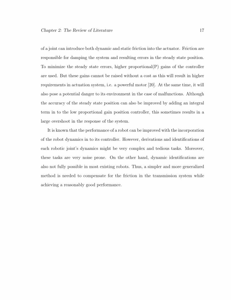
Chapter 2: The Review of Literature 17
of a joint can introduce both dynamic and static friction into the actuator. Friction are
responsible for damping the system and resulting errors in the steady state position.
To minimize the steady state errors, higher proportional(P) gains of the controller
are used. But these gains cannot be raised without a cost as this will result in higher
requirements in actuation system, i.e. a powerful motor [20]. At the same time, it will
also pose a potential danger to its environment in the case of malfunctions. Although
the accuracy of the steady state position can also be improved by adding an integral
term in to the low proportional gain position controller, this sometimes results in a
large overshoot in the response of the system.
It is known that the performance of a robot can be improved with the incorporation
of the robot dynamics in to its controller. However, derivations and identifications of
each robotic joint’s dynamics might be very complex and tedious tasks. Moreover,
these tasks are very noise prone. On the other hand, dynamic identifications are
also not fully possible in most existing robots. Thus, a simpler and more generalized
method is needed to compensate for the friction in the transmission system while
achieving a reasonably good performance.

Chapter 3
Modelling and Control
3.1 Introduction
This chapter will describe the modelling of the actuators under loading condition as
well as appropriate control laws used to achieve good performance and stability. The
modelling of both Rotary Elastic Actuator (REA) and Rigid Actuator (RA) will be
considered here. The control laws which are used by the actuators are Computed
Torque Control and Proportional-Integral-Derivative (PID) for position and torque
control respectively. While, PID and Hybrid Speed/Force control will be used to
control the output force of the actuators.
3.2 Model of Actuator
3.2.1 Rigid Actuator(RA)
A rigid actuator is made up of a motor coupled with a gearbox and the output shaft
connected directly to the load. The purpose of a gearbox is to increase the output
torque and step down the speed. However, frictions in the gearbox will decrease the
18

Chapter 3: Modelling and Control 19
efficiency of the motor drive system and affect the performance of the actuator.
Gearbox
Motor
Motor Encoder
Coupler
Output Encoder
Output Load
Figure 3.1: Rigid Actuator
Figure 3.1 shows a picture of rigid rotary actuator with an output load, which is
modelled as a simple pendulum. While, Figure 3.2 shows its corresponding model.
The motor and gearbox combination is modelled as a low speed, high torque motor
taking into considerations such as the frictions of the gearbox and the inertia of the
motor.
The dynamics of the Rigid Actuator (RA) can be derived from Newton’s Law and
Laplace Transform, as follows:
τm − τL − τfr = Jθm (3.1)

Chapter 3: Modelling and Control 20
3
As far as the torque control is concerned, the elastic flywheels are not only capable of giving a control system that delivers an accurate output torque, but the elastic elements are also shock absorbers. Thus, impact force transmitted to the motor wil l be greatly reduced and stored in the springs as potential energy. Furthermore, this actuator is capable of multi-revolution. As different applications may require different specified performance criteria, the elastic flywheels are designed to accommodate different spring stiffness, which in turn make up the overall stiffness of the actuator. Since the extension springs used in the flexible flywheels are stock springs, this means they are easily available and have a variety of stiffness. This is a very favorable factor in the commercial or industrial area.
III Model of Actuator
III.1 Rigid Actuator
A rigid actuator is made up of a motor coupled
with a gearbox and the output shaft connected directly to the load. The purpose of a gearbox is to increase the output torque and step down the speed. However, frictions in the gearbox will decrease the efficiency of the motor drive system and affect the performance of the actuator.
Figure 5 showed a rigid rotary actuator with the load applied to the actuator is modeled as a simple pendulum. The motor and gearbox combination is modeled as a low speed, high torque motor [8], taking into considerations such as the frictions of the gearbox
and the inertia of the motor. Thus, mτ is the torque
applied to the motor, Jm is the inertia of the motor,
Lτ is the output torque, frτ is the frictional torque,
which made up of both static or holding, sfτ and
dynamic term, •
∗θb and θ is the angular position of both motor and load.
Figure 5 Model of a Rigid Actuator
By applying Newton’s Law and Laplace Transform,
••=−− mmfrLm J θτττ (6)
mbsffr
•∗+= θττ (7)
••= LL ml θτ 2
(8) •
∗+++= θτθτ sbsJmlsss sfmm )())(()( 22 (9)
III.2 Elastic Actuator
Like Rigid Actuator, an Elastic Actuator requires motor and gearbox with an additional of a flexible flywheel, which is used as torque feedback.
Figure 6 Model of the Rotary Elastic Actuator with Load.
In this case, the angular position of the motor, mθ
and the output load, Lθ is different due the elasticity of the elastic flywheel. Equations (6), (7), (8) and (9) also apply to the elastic model with the additional of
)( LmSL K θθτ −= (10)
IV Control
IV.1 Position Control
Computed Torque control [9] is used to control
the positioning of the actuator. It is a control law which computes torque applied by the actuator as a function of the sensed feedback as:
βαττ += 'm (11)
Compare equation (9) and (11) and let •••
∆−∆−== θθθτ KvKp' (12)
Thus, )(
2
ssb
mlJm
sf θτβα
∗+=+=
(13)
frτ
Lθ Ks
Mθ
mτ
frτ
mτ
Lθ
Lτ
g
J
m
J Lτ
m g
Figure 3.2: Model of Rigid Actuator
τfr = τsf + b ˙θm (3.2)
τL = ml2θ̈L + mglsinθL (3.3)
Since θm=θL, let θ = θm = θL:
τm(s) = s2θ(s)(ml2 + J) + bsθ(s) + mglsinθ(s) (3.4)
where τm is the torque applied to the motor, J is the inertia, τL is the output
torque, τfr is the frictional torque, which made up of both static or holding torque,
τsf and the dynamic friction term, bθ̇ and θ is the angular position of both motor and
load. The gravitational term is made up of mass of load (m), gravitational constant
(g), leverage (l) and θ.
The ”dead zone” as shown in Figure 3.3 is used to simulate the static friction of
the gearbox. Refer to Figure 3.3 for the model of Rigid Actuator. The actuator will
not rotate if the command torque is lower than the range of the static torque. While,

Chapter 3: Modelling and Control 21
Output Torque
OUTPUT DYNAMICS +
MOTOR DRIVE DYNAMICS
Modelling of REA
Motor Torque
Speed
Position
Output Torque
Quantizer(due to encoder)
1s
Int.
1s
Int
f(u)
Grav. Term
Dead Zone(Holding Torque)
-K-
Damping from
Gearbox
-K-
1 / (Motor Drive Inertia
+ Load Inertia)
Figure 3.3: Modelling of Rigid Actuator using SimuLink
the ”quantizer”block set is to simulate the quantization effect of an optical encoder
due to its digital nature.
3.2.2 Elastic Actuator(EA)
There are numerous ways can be used to achieve elasticity in an actuator. Typical
components or material used are soft rubber, plastic and dampers. However, springs
are chosen as the compliant material to provide elasticity for this actuator. The
detailed design of the Elastic Actuator will be discussed in Chapter 4.
Like Rigid Actuator, an Elastic Actuator also requires motor and gearbox with
an additional of a flexible flywheel, which is used as torque feedback and provides
elasticity into the system. The Elastic Actuator and its corresponding dynamics
model are shown in Figure 3.4 and 3.5 respectively.
For Elastic Actuator(EA), the angular position of the motor, θm and the output
load, θL are different due the elasticity of the elastic flywheel. Equations 3.1, 3.2,
3.3 and 3.4 also apply to the elastic model with the additional of τL = Ks(θm − θL),

Chapter 3: Modelling and Control 22
Gearbox
Motor
Motor Encoder
Coupler
Elastic Flywheel
Output Encoder
Output Load
Figure 3.4: Rotary Elastic Actuator
3
As far as the torque control is concerned, the elastic flywheels are not only capable of giving a control system that delivers an accurate output torque, but the elastic elements are also shock absorbers. Thus, impact force transmitted to the motor wil l be greatly reduced and stored in the springs as potential energy. Furthermore, this actuator is capable of multi-revolution. As different applications may require different specified performance criteria, the elastic flywheels are designed to accommodate different spring stiffness, which in turn make up the overall stiffness of the actuator. Since the extension springs used in the flexible flywheels are stock springs, this means they are easily available and have a variety of stiffness. This is a very favorable factor in the commercial or industrial area.
III Model of Actuator
III.1 Rigid Actuator
A rigid actuator is made up of a motor coupled
with a gearbox and the output shaft connected directly to the load. The purpose of a gearbox is to increase the output torque and step down the speed. However, frictions in the gearbox will decrease the efficiency of the motor drive system and affect the performance of the actuator.
Figure 5 showed a rigid rotary actuator with the load applied to the actuator is modeled as a simple pendulum. The motor and gearbox combination is modeled as a low speed, high torque motor [8], taking into considerations such as the frictions of the gearbox
and the inertia of the motor. Thus, mτ is the torque
applied to the motor, Jm is the inertia of the motor,
Lτ is the output torque, frτ is the frictional torque,
which made up of both static or holding, sfτ and
dynamic term, •
∗θb and θ is the angular position of both motor and load.
Figure 5 Model of a Rigid Actuator
By applying Newton’s Law and Laplace Transform,
••=−− mmfrLm J θτττ (6)
mbsffr
•∗+= θττ (7)
••= LL ml θτ 2
(8) •
∗+++= θτθτ sbsJmlsss sfmm )())(()( 22 (9)
III.2 Elastic Actuator
Like Rigid Actuator, an Elastic Actuator requires motor and gearbox with an additional of a flexible flywheel, which is used as torque feedback.
Figure 6 Model of the Rotary Elastic Actuator with Load.
In this case, the angular position of the motor, mθ
and the output load, Lθ is different due the elasticity of the elastic flywheel. Equations (6), (7), (8) and (9) also apply to the elastic model with the additional of
)( LmSL K θθτ −= (10)
IV Control
IV.1 Position Control
Computed Torque control [9] is used to control
the positioning of the actuator. It is a control law which computes torque applied by the actuator as a function of the sensed feedback as:
βαττ += 'm (11)
Compare equation (9) and (11) and let •••
∆−∆−== θθθτ KvKp' (12)
Thus, )(
2
ssb
mlJm
sf θτβα
∗+=+=
(13)
frτ
Lθ Ks
Mθ
mτ
frτ
mτ
Lθ
Lτ
g
J
m
J Lτ
m g
Figure 3.5: Model of Rotary Elastic Actuator

Chapter 3: Modelling and Control 23
ELASTICFLYWHEEL
Output Torque
Output Position
MOTOR DRIVE SYSTEM
OUTPUT DYNAMICS
Modelling of REA
Motor Torque
Static Friction
Quantizer1 Quantizer
-K-
Motor Drive
Inertia 1s
Int6
1s
Int5
1s
Int4
1s
Int2
f(u)
Grav. Term
E F
E
-K-
Dynamic Friction
-K-
1/Load Inertia
Figure 3.6: Modelling of Rotary Elastic Actuator using SimuLink
which models the torque measured by the Elastic Flywheel. Figure 3.6 shows the
architecture of Rotary Elastic Actuator with output load as modelled by SimuLink.
Thus, the equations represent the Rotary Elastic Actuator are as below:
τm(s) = s2[Jθm(s) + ml2θL(s)] + bsθ(s) + mglsinθL(s) (3.5)
τL = Ks(θm(s)− θL(s)) (3.6)
3.3 Control
There are three type of control algorithms which are used to control the actuators.
Depending on the application of the robots, these actuators are capable of performing
position, torque and force control. However torque control is only performed on
Rotary Elastic Actuator(REA) as shown in Chapter 5. The main purpose of these
control algorithms are to compare the performance of both Rigid and Elastic Actuator
in position and force/torque control.

Chapter 3: Modelling and Control 24
3.3.1 Position Control of Rigid Actuator(RA)
Computed Torque Control[23] is used to control the positioning of the actuator. It is
a control law which computes torque applied by the actuator as a function of sensed
feedback.
τm = ατ′+ β (3.7)
Compare Equation 3.4 and 3.7 and let
τ′= −Kp∆θ −Kv∆θ̇ (3.8)
Thus,
α = J + ml2 (3.9)
J = Jm + n2Jgb (3.10)
β = τsf (s) + bsθ(s) + mglsinθL(s) (3.11)
,where n = gearbox ratio, Jgb = inertia of gearbox,Jm = inertia of motor, Kp, Kv
= controller’s gain, ∆θ = the difference between the desired position and output
position and ∆θ̇ = the difference between the desired velocity and output velocity.
From the equations computed (Equations 3.8 - 3.11), the position control archi-
tecture of a Rigid Actuator is represented by Figure 3.7. Refer to Chapter 5for the
performance of the Rigid Actuator.
3.3.2 Position Control of Rotary Elastic Actuator(REA)
It is proven that the performance of an actuator can be improved by closing the loop
between the motor and its end point. The position control of the REA as shown

Chapter 3: Modelling and Control 25
Output Torque
OUTPUT DYNAMICS +
MOTOR DRIVE DYNAMICS
Modelling of REA
Motor Torque
Speed
Position
Output Torque
COMPUTED TORQUE
CONTROL
Quantizer
(due to encoder)
-K-Kv
388Kp
1s
Int.
1s
Int
f(u)
Grav. Term
DesirePosition
Dead Zone(Holding Torque)
-K-
Damping from
Gearbox
-K-
1 / (Motor Drive Inertia
+ Load Inertia)1
-K-
1 / (Motor Drive Inertia
+ Load Inertia)
Figure 3.7: Position Control Architecture of Rigid Actuator
in Figure 3.8 will incorporate an inner loop PID torque control into the original
computed torque control.
The inner loop torque control will modulate an output torque based on the differ-
ence between the torque commanded by the computed torque control and the actual
output torque at its end point. This control system is also used to compensate the
softness of the actuator to a certain extent. The equation used for the inner loop PID
torque control is shown as below:
τm =Kps + Kvs
2 + KI
s(τ − τL) (3.12)
where KP = Proportional gain, KV = Derivative gain, KI = Integral gain, τ =
Torque commanded by Computed Torque Control, τL = Output load (Refer Equation
3.6) and τm = Motor torque.

Chapter 3: Modelling and Control 26
ELASTICFLYWHEEL
Gravitational Term
T
INNER LOOP PID TORQUE
CONTROL
Output Torque
Output Position
Output Velocity
COMPUTED TORQUE
CONTROL
MOTOR DRIVE SYSTEM
OUTPUT DYNAMICS
COMPUTED TORQUE CONTROL WITH INNER LOOP PID TORQUE CONTROL
Without Inner Loop
Static Friction
Quantizer1 Quantizer
-K-
Motor Drive
Inertia -K-
LoadInertia
-K-Kv
3Kp
1s
Int6
1s
Int5
1s
Int4
1s
Int2
PID
Inner Loop PID
f(u)
Grav. Term
E F
E
-K-
Dynamic Friction
Desire
-K-
1/Load Inertia
Figure 3.8: Position Control Architecture of Rotary Elastic Actuator
3.3.3 Torque Control
The control of torque in the robotic joints will ultimately lead to the control of force
at the end effector of a robot. PID torque control is used to control the output torque
of the elastic actuator. The PID controller here is similar to the inner loop PID torque
controller in Equation 3.12, except in this case, the output torque will be compared
with a desired torque as shown in Equation 3.13.
τm =Kps + Kvs
2 + KI
s(τD − τL) (3.13)
where τD = desired torque.
The torque control architecture of Rotary Elastic Actuator is shown in Figure 3.9.
The performances of the Rotary Elastic Actuators are presented in Chapter 5. These
performances are based on the results obtained from simulations as well as real life
experiments.

Chapter 3: Modelling and Control 27
ELASTICFLYWHEEL
PID TORQUECONTROL
Output Torque
Output Position
MOTOR DRIVE SYSTEM
OUTPUT DYNAMICS
Static Friction
Quantizer1 Quantizer
-K-
Motor Drive
Inertia
1s
Int6
1s
Int5
1s
Int4
1s
Int2
PID
Inner Loop PID
f(u)
Grav. Term
E F
E
-K-
Dynamic Friction
DesireTorque
-K-
1/Load Inertia
Figure 3.9: Torque Control Architecture of Rotary Elastic Actuator
3.3.4 Force Control: Contact Start
There are two type of force control commonly used in robotic system. The first
type is a force control with its end-point contacting the working surface. While, the
latter is a force control with its end-point initially moving towards a working surface
and ultimately in contact with the surface to generate a desired output force. This
controller is particularly useful in applications such as blind walking of biped where
the biped are designed to walk on unknown terrain and experience unexpected impact.
In general , force control started with contacting to a surface is easier to implement
and stabilize than those moving towards contact surfaces.
Similar to Torque Control, PID is used to control the force at the point of contact
between the actuator and the working surface. The force controller computes a motor
torque, τm (Equation 3.14) based on the difference between the desired force, FD and
the contact force, FL. A simple load cell is used to measure the contact force and

Chapter 3: Modelling and Control 28
thus providing force feedback into the control loop. Refer to Figure 3.10 for the force
control architecture of Rigid Actuator in contact with surface.
Output Position
FORCE CONTROL
MOTOR DRIVE SYSTEM + OUTPUT DYNAMICS
Contact Force
Tm
Dynamic Compensation
Static Friction
PID
Outer Loop PID
f(u)
Load Cell
1s
Int4
1s
Int2
f(u)
Grav. Term
-K-
Gain
-K-
Dynamic Friction
DesiredForce
-K-
1/Load Inertia
Figure 3.10: Force Control Architecture of Rigid Actuator in Contact with Surface.
τm =Kps + Kvs
2 + KI
s(FD − FL) (3.14)
In addition to the outer loop PID force control (Equation 3.15), the inner loop
torque control (Equation 3.16) similar to Equation 3.12 will also be implemented into
the force controller of REA. Refer to Figure 3.11 for the force control architecture of
REA in contact with surface.
τO =Kps + Kvs
2 + KI
s(FD − FL) (3.15)
τm =Kps + Kvs
2 + KI
s(τO − τL) (3.16)

Chapter 3: Modelling and Control 29
ELASTICFLYWHEEL
INNER LOOP PID TORQUE
CONTROL
MOTOR DRIVE SYSTEM
OUTPUT DYNAMICS
Tm
Output Position
Output Torque
Contact Force
FORCE CONTROL
To Static Friction
Quantizer1 Quantizer
PID
Outer Loop PID
-K-
Motor Drive
Inertia
f(u)
Load Cell
1s
Int6
1s
Int5
1s
Int4
1s
Int2
PID
Inner Loop PID
f(u)
Grav. Term
-K-
Gain
E F
E-K-
Dynamic Friction
DesiredForce1
-K-
1/Load Inertia
Figure 3.11: Force Control Architecture of Rotary Elastic Actuator in Contact withSurface.
, where τO = the torque computed by the Outer Loop Force Control and τL = the
output torque measured by the Elastic Flywheel.
3.3.5 Force Control: Moving to Contact
When the actuator is moving in free space, the response of the actuator under the
PID controller used for force control in Sect. 3.3.4 can be quite slow. Although the
gains can be increased to speed up the positional response, the impact force will be
also be greatly increase by doing so. Furthermore, it might cause instability of the
robot upon an impact. Thus, hybrid speed/force control is used. As the actuator is
moving towards the contact surface, speed control under Computed Torque Control
(refer to Equations 3.17 to 3.21) will be used.
For Contact Force, FL ≤ 0.5N, then Speed Control:

Chapter 3: Modelling and Control 30
τm = ατ′V + β (3.17)
Compare Equation 3.4 and 3.17 and let
τ′V = −Kv∆θ̇ (3.18)
Thus,
α = J + ml2 (3.19)
J = Jm + n2Jgb (3.20)
β = τsf (s) + bsθ(s) + mglsinθL(s) (3.21)
,where τ′V = the torque computed by Computed Torque Control for Speed Control,
n = gearbox ratio, Jgb = inertia of gearbox,Jm = inertia of motor, Kv = controller’s
gain and ∆θ̇ = the difference between the desired velocity and output velocity.
Once there is a contact between the actuator and the surface i.e. the impact force
exceeded 0.5 N, the controller will switch over to the PID force control (Equation
3.22) which is described in Sect.3.3.4 previously .
For Contact Force, FL > 0.5N, then Force Control:
τm =Kps + Kvs
2 + KI
s(FD − FL) (3.22)
Refer to Fig.3.12 and Fig.3.13 for the Force Control of Rigid Actuator and Rotary
Elastic Actuator(REA) moving to contact respectively. The Outer Loop Force Con-
trol of REA moving to contact surface will be the same as the Hybrid Speed/Force
Control used in the Rigid Actuator. An Inner Loop PID Torque Control will be

Chapter 3: Modelling and Control 31
incorporated into the Force Control of REA moving to contact surface as shown in
Equations 3.23.
τm =Kps + Kvs
2 + KI
s(τO − τL) (3.23)
, where τO = the torque computed by the Outer Loop Force Control and τL = the
torque measured by the Elastic Flywheel. Refer to Figure 3.13.
HYBRID SPEED/ FORCE CONTROL
Output Position
Contact Force
MOTOR DRIVE SYSTEM + OUTPUT DYNAMICS
Tm
Dynamic Compensation
Output Velocity
Static Friction
else
Vd
tl
Vl
T
SpeedController
f(u)
Load Cell1
1s
Int3
1s
Int1
u1
if(u1>0.5)
elseif(u1<-0.5)
else
Hybridf(u)
Grav. Term1
-K-
Gain
Fl
Fd
if
else if
T
ForceController
-K-
Dynamic Friction
DesiredSpeed
DesiredForce -K-
1/Load Inertia1
Figure 3.12: Force Control Architecture of Rigid Actuator Moving to Contact.
The advantage of using hybrid speed/force control is that the maximum impact
force can be controlled to a certain extent by controlling the speed of the actuator just
before it came into contact with the working environment. The impact force can be
reduced by decreasing the desired speed. But this will contribute to the sluggishness
of the actuators’ response. Thus the impact force and the desired speed have to
be optimized in order to achieve an appropriate force response when the actuator is

Chapter 3: Modelling and Control 32
ELASTICFLYWHEEL
INNER LOOP PID TORQUE
CONTROL
HYBRID SPEED/ FORCE
CONTROL
MOTOR DRIVE SYSTEM
OUTPUT DYNAMICS
Tm
To
Output Position
Output Velocity
Output Torque
Contact Force
Static Friction
else
Vd
Vl
tl
T
SpeedController
Quantizer1 Quantizer
-K-
Motor Drive
Inertia
f(u)
Load Cell
1s
Int6
1s
Int5
1s
Int4
1s
Int2
PID
Inner Loop PID
u1
if(u1>0.5)
elseif(u1<-0.5)
else
Hybrid
f(u)
Grav. Term
-K-
Gain
Fl
Fd
if
else if
T
ForceController
E F
E-K-
Dynamic Friction
DesiredSpeed
DesiredForce
-K-
1/Load Inertia
Figure 3.13: Force Control Architecture of Rotary Elastic Actuator Moving to Con-tact.
initially not in contact with the working surface.

Chapter 4
Actuator Design
4.1 Introduction
This chapter describes the design and construction of the Rotary Elastic Actua-
tor (REA). As discussed previously in Chapter 2 there are a few ways to achieve
force/torque control while adding elasticity into the system. The flywheel design is
chosen here because of its modularity and its elegance way of computing torque from
the elongation and contraction of the springs. The details of the torque computation
will be discussed in Section 4.3. In addition, this design is also capable of adding
elasticity into the actuator and accurate torque generation, which in turn can be
used to improve the positioning control. As far as the modularity of the design is
concerned, it is designed to implement in most of the existing actuators such as direct
drive robots. Figure 4.1 shows a photograph of the Rotary Elastic Actuator (REA)
realized and used in the experimental setup. However the first prototype of REA will
be very flexibly designed to suit a wide range of loading conditions for the purpose of
experiment . Thus, the size of REA might appear to be slightly bulky at the moment.
However, suggestions to further reduce the size of the actuator will be discussed in
33

Chapter 4: Actuator Design 34
the later part of this thesis.
Bearing Support Units
Output Load
Gearbox
Elastic Flywheel
Coupling
Output Encoder
Motor
Motor Encoder
Motor Driver
Figure 4.1: A photograph of Rotary Elastic Actuator
Rotary Elastic Actuator consists of a servomotor coupled with a gearbox, a cou-
pler, the Elastic Flywheel(EF ), bearing support units and encoders. The maximum
detectable range of the actuator’s output torque depends on the stiffness of the exten-
sion springs it used. The relationship between the output torque range and the spring
stiffness will be discussed in the later part of this chapter. The following sections of
this chapter will describe in detail the power-train system, the design of the elastic
flywheel, the choice of sensors used, the control hardware that was used as well as
the control algorithms implemented on the actuator.

Chapter 4: Actuator Design 35
4.2 The Power-train System
The selection of the power-train system, which is the combination of motor with
gearbox, depends on the maximum output torque and speed required. Since the
Rotary Elastic Actuator (REA) is designed mainly for experimental purposes, the
system is chosen to produce around 50 Nm of continuous torque at a speed of around
80 rpm. In addition, gearbox is chosen according to its efficiency and back-drivability.
Details of the chosen combination of power-train system are shown in Tables 4.1 and
4.2.
SpecificationPower 400 WTorque 1.3 Nm (Continuous), 5.0 Nm (Stall)Weight 750 GmCurrent 2.5 A (Continuous), 10.5 A (Maximum)Inertia 0.36 x 10⁻⁴ kgm−2
No load Speed 5000 rpm
Table 4.1: Specification of Panasonic Servo Motor MSDA043A1A
SpecificationReduction Ratio 40 : 1Torque 60 Nm (Continuous), 200 Nm (Maximum)Efficiency 92Weight 1.5 KgSpeed @ 50 Nm 76.4 rpmInertia 0.28 x 10⁻⁴ kgm−2
Table 4.2: Specification of ZF PG50/100-040 Gearbox
The servomotor comes with a 2500 quadrature pulse per revolution (ppr) encoder.
This encoder is used to measure the position of the motor shaft and served as part
of the torque sensor system. Since a 40:1 ratio step down gearbox and quadrature
decoding is used ot enable higher resolution, the output position of the powertrain

Chapter 4: Actuator Design 36
system will have a maximum resolution of (40 x 2500 x 4) pulses per revolution
(ppr), which is equivalent to 0.001 degree. The gearbox selected is claimed by the
manufacturer to have close to zero backlash and have an efficiency of 92 percent.
4.3 Elastic Flywheel Design
As far as robotic applications are concerned, contacts between its end effectors with
working surfaces are always unavoidable. Thus, some sort of elasticity between the
robotic structure and its contact surface are needed. In addition, torque sensory sys-
tem is also required in order for the actuator to detect certain motions, which are
used as feedback to the control loop. So, the Elastic flywheel is designed to accommo-
date these two requirements. The Elastic Flywheel is made up of extension springs,
flywheels, bearings and bushes for smooth rotation while fastener and connectors to
hold the whole structure in place.
In a Rotary Elastic Actuator, an electric motor-gearbox combination is used to
drive the motor flywheel, which transmits a torque to drive the output flywheel
through the extension springs. The output flywheel is then connected to the out-
put load. The arrangement of the springs between the motor flywheel and the output
flywheel can be viewed more clearly in Figure 4.2.
In Figure 4.2, an eight springs, rotary elastic actuator is shown and the motor
flywheel is hidden for the ease of understanding. Initially, the springs are pre-extended
to their mid-extension length to allow torque measurements in both clockwise and
anti-clockwise directions. When there is an input torque generated by the actuator,
four alternately arranged springs (i.e. Spring 1) will be extended over their mid
extension points, while the other four alternately arranged springs(i.e. Spring 2) will

Chapter 4: Actuator Design 37
Connect to Motor Shaft
Extension Spring
Spring Length Adjuster
Spring Slider
Angular Limiter
Connect to Output Load
Figure 4.2: Front View and Isometric View of Elastic Flywheel
Attached to Output Flywheel
Attached to Motor Flywheel
Rad
ius,
R Relative angle
Final Length of Spring 1
Final Length of Spring 2
Initial Length of Spring 1
Initial Length of Spring 2
a
t
Figure 4.3: Schematic Diagram of a Quarter of the Elastic Flywheel before and Afterthe Transmission of Torque

Chapter 4: Actuator Design 38
be extended under their mid-extension point.
To calculate the length of the spring, encoders are used to measure the angular
position of the motor flywheel and the output flywheel respectively. Instead of using
strain gauges, which are very noise prone, encoders are used to maintain the accuracy
of the measurements. Figure 4.3 shows a quarter of the Elastic Flywheel schematically.
F1 = KS[2R
cosasin(
π
ns
− a− ∆θ
2)]− Lfl1 (4.1)
F2 = KS[2R
cosasin(
π
ns
− a +∆θ
2)]− Lfl2 (4.2)
τ1 = F1cos(π
ns
− a− ∆θ
2)
R
cosa(4.3)
τ2 = F2cos(π
ns
− a +∆θ
2)
R
cosa(4.4)
τ =ns
2(τ2 − τ1) (4.5)
Symbol DefinitionR Radiusns No. of springLfln Free length of spring, n=1,2.a tan−( t
R)
∆θ Relative angleKS Stiffness of SpringFn Force in springτn Torque generated by each springτ Net Torque
Table 4.3: Definition of Symbols

Chapter 4: Actuator Design 39
By measuring the angular position between the output and the motor, the length
of the springs can be calculated using geometrical equations and the overall torque
that is being transmitted can then be computed as in Equations 4.1 - 4.5, with Table
4.3 explaining the symbols used.
The accuracy of the output torque relies heavily on the accurate response of the
spring under loading conditions. As far as the linear extension range of the springs are
concerned, angle limiters are installed in the core of the elastic flywheel to ensure the
maximum and minimum operating lengths of the springs are not exceeded under any
loading condition. Figure 4.4 shows the configuration of the angular limiter between
the flywheels in detail.
A deep groove ball bearing and a thrust bearing are used to provide smooth
relative rotation between the flywheels and maintain a consistent gap between the
two flywheels. To further reduce the frictional errors in the system, dry running
bushes are placed between the loop end of each spring and the screws that hold the
spring to its holder. Refer to Figure 4.5 for the configuration of the spring-slider
assembly.
For the purpose of experimental work, the first prototype of the rotary elastic
actuator will be very modularly designed to suit a wide range of loading conditions.
For example, if an application requires a high torque operation, then a stiffer spring
will be used. Thus, large flywheels are designed to accommodate a wide range of
extension springs. However there is always a compromise between the resolution of
the torque generated and its maximum detectable range. The relationship between
the spring stiffness and the characteristics of the actuator will be discussed in the
next section. Refer to AppendixA for the technical drawings of the actuator.

Chapter 4: Actuator Design 40
)]2
sin[cos
2( 11 fls Ln
piRKF −∆−−= θα
α (Eqn. 4.1)
)]2
sin[cos
2( 22 fls Ln
piRKF −∆+−= θα
α (Eqn. 4.2)
αθατ
cos)
2cos(11
R
n
piF
∆−−= (Eqn. 4.3)
αθατ
cos)
2cos(22
R
n
piF
∆+−= (Eqn. 4.4)
)(2 12 τττ −= n
net (Eqn. 4.5)
The accuracy of the output torque relies heavily on the accurate response of the spring
under loading conditions. As far as the linear extension range of the springs are
concerned, angle limiters are installed in the core of the elastic flywheel to ensure the
maximum and minimum operating lengths of the springs are not exceeded under any
loading condition. Figure 4.5 shows the configuration of the angular limiter between
the flywheels in detail.
Fig. 4.5 The Configurations of Angular Limiters Between The Flywheels.
A deep groove ball bearing and a thrust bearing are used between the flywheels to
provide smooth rotation relative each other and maintain a consistent gap between the
two flywheels. To further reduce the frictional errors in the system, dry running
Figure 4.4: The Configuration of Angular Limiters Between the Flywheels.
31
A deep groove ball bearing and a thrust bearing are used between the flywheels to
provide smooth rotation relative each other and maintain a consistent gap between the
two flywheels. To further reduce the frictional errors in the system, dry running bushes
are placed between the loop end of each spring and the screws that hold the spring to its
holder. Refer to Fig. 4.6 for the configuration of the spring-slider assembly.
Fig. 4.6 The Exploded View of The Spring-slider Configuration.
For the purpose of experimental work, the first prototype of the rotary elastic actuator
will be very modularly designed to suit a wide range of loading conditions. For example,
if an application requires a high torque operation, then a stiffer spring will be used. Thus,
large flywheels are designed to accommodate a wide range of extension springs.
However there is always a compromise between the resolution of the torque generated
and its maximum detectable range. The relationship between the spring stiffness and the
characteristics of the actuator will discuss in the next section.
4.4 Characteristic of Elastic Flywheel
Figure 4.5: The Exploded View of The Spring-slider Configuration.

Chapter 4: Actuator Design 41
4.4 Characteristic of Elastic Flywheel
The characteristics of the elastic flywheel depend on the extension spring it used.
Table 4.5 shows the characteristic of the elastic flywheel versus the extension springs
as calculated using Equations 4.1 - 4.5. While Table 4.4 is the characteristic of the
extension springs supplied by Associated Spring[24]. Part numbers in Tables 4.4 and
4.5 are for the extensions manufactured by Associated Spring.
Extension springPart No. Diameter Free Length Max. Extension Stiffness Max. Force
(mm) (mm) (mm) (N/mm) (N)T42340 14 50.0 23.60 5.88 164T42430 20 48.0 10.10 21.90 259T42660 14 44.2 7.65 44.60 400T42690 20 53.8 20.30 12.30 293
Table 4.4: Characteristic of Extension Spring
Elastic FlywheelPart No. Rel. Angle Stiffness Max. Torque Resolution
(deg) (Nm/deg) (Nm) (Nm/pulse)T42340 ±7.56 5.97 ±45.14 0.21T42430 ±3.78 17.24 ±65.20 0.62T42660 ±2.7 30.21 ±81.64 1.09T42690 ±6.12 13.39 ±81.88 0.48
Table 4.5: Characteristic of Elastic Flywheel.
Table 4.4 and 4.5 show that the stiffness of the elastic flywheel is directly propor-
tional to the stiffness of the extension springs used. As far as the range of detectable
torque is concerned, extension springs which are short in lengths but capable of long
extensions are desire. But as a matter of fact, short springs tend to be very stiff and
their lengths of extensions are also shorter. In other words, as the stiffness of the
elastic flywheel increases, its resolution in torque generation will decrease at the same

Chapter 4: Actuator Design 42
time. The stiffness of the elastic flywheel is inversely proportional to its resolution.
The calculation of the resolution of the elastic flywheel is based on 10000 pulses per
revolution (ppr) encoders. From Table 4.5, it shows that the stiffness of the elastic fly-
wheel will affect the resolution of the actuator in torque generation. If the actuator is
needed to generate torque with finer resolution, higher resolution encoders or encoder
signal interpolators are then required. Alternatively, softer extension springs can be
used to construct a softer elastic flywheel. However, high resolution can sometimes
be redundant in certain robotic applications and the performance of an actuator also
depends on the stiffness of the elastic flywheel. Excessive of softness in actuator can
cause the performance to be somehow sluggish and hard to stabilize the system.
4.5 Sensor System
The Elastic Flywheel which provides elasticity for the actuator also made up part
of the torque sensory system. As shown in the previous section, the amount of the
torque generated by the actuator can be computed by the angle of twist of the elastic
flywheel. Thus, the accuracy of the computed torque depends on how well the angular
positions of both the motor end and the output end are being sensed.
4.5.1 Method of Sensing
As far as calculating the output toque of the actuator is concerned, there are two
methods of sensing the angle of twist. The first method would be to measure the
angular positions of the motor end and the output end respectively and then, calculate
the angle of twist by subtracting the two readings.

Chapter 4: Actuator Design 43
Alternately, a position sensor can be installed in between the two flywheels to
measure the relative angular position of the flywheels. Since this actuator is also
designed for position control, there will be another sensor needed to sense the actual
output position of the actuator.
Thus, the first method was chosen as the mounting of sensors onto the actuator
is much simpler than the the latter. This is also due to the fact that the servomotor
already comes with an encoder. Refer to Figure 4.6 for the schematic layout of the
Rotary Elastic Actuator. So all that is needed here is to install another sensor at the
output end. On the other hand, the mechanical design to accommondate a relative
sensor in between the flywheels will also be a very complex one. Furthermore, the
wiring of these sensors can also limit the actuator from making a full revolution.
Other considerations such as the ease of assembly , cost and machinability of parts
also favor the first method.
4.5.2 Choice of Sensors
There are three types of sensors that can be used in this application. Namely, opti-
cal encoder, strain gauge and potentiometer. Optical encoders are by far the most
suitable choice for this application. This is because optical encoder signals are digital
and less noisy. Also, due to the fact that strain gauges and potentiometers are inher-
ently analog sensors which means their signals are generally noise prone. Thus extra
circuits are needed to filter these signals and convert them into digital. In spite of
their noise prone nature, these sensors also give small readings down to a few microns
for a relatively large deflection which make them potentially inaccurate in certain ap-
plications. The messy wiring of strain gauges also can limit the degree of revolution

Chapter 4: Actuator Design 44
Gearbox
Motor
Motor Encoder
Coupler
Elastic Flywheel
Output Encoder
Output Load
Figure 4.6: The Schematic Layout of Rotary Elastic Actuator (REA).
of the actuator.
Thus, optical encoders are chosen on the basis that they are inherently easier to
use, more compatible to this setup and potentially more accurate than the strain
gauges and potentiometer.
4.6 Testing of Elastic Flywheel
In order to test the accuracy of the torque computed using the Elastic Flywheel, a
simple test is conducted. Refer to Figure 4.7 for the layout of the test use to verify the
accuracy of Elastic Flywheel in torque feedback. The motor shaft is held stationary
by engaging its mechanical clamp. The torque computed by the Elastic Flywheel
using Equation 4.1-4.5 will be compared against the actual torque applied to the

Chapter 4: Actuator Design 45
Gearbox
Motor with mechanicalclamp engaged
Motor Encoder
Coupler
Elastic Flywheels (EF)Output Encoder
Applied Mass, m
Leverage, l
Figure 4.7: The Layout of the Test for Elastic Flywheel.
output end of the actuator according Equation 4.6.
τg = mglsinθL (4.6)
,where the actual torque, τg applied to the actuator is simply a known mass, m applied
to at a certain leverage, l with respect to the output axis of the actuator.
From Figure 4.8 the torque measured by the Elastic Flywheel varies linearly with
the applied torque. There are slight non-linearity found in results, which could due to
the frictional errors in the elastic flywheel and the quantization effects of the encoders.
However, these non-linearities are very small and thus, it is still acceptable in most
of the robotic applications.

Chapter 4: Actuator Design 46
Measured Torque vs. Applied Torque
-30
-20
-10
0
10
20
30
-30 -20 -10 0 10 20 30
Applied Torque, Tap (Nm)
Mea
sure
d T
orq
ue,
Ts
(Nm
)
Experimental Results
Theorectical
Figure 4.8: Measured Torque against Actual Torque.

Chapter 4: Actuator Design 47
Window Base PC with Real-time Extension (RTX)
Servo Togo Card
Motor Driver
E Motor - Gearbox
E
M
Elastic Flywheel
Window Base PC with Real-time Extension (RTX)
Servo Togo Card
70 Motor Driver
E Motor - Gearbox
E
M
100
90
80 40
23
31
Figure 4.9: The Block Diagram of Experiment Setup.
4.7 Experiment Setup
This section will describe the electronics and control hardware used to set up the
test rig for the experiment. Although the experiment setups for both position and
force/torque control are the same, the control algorithms implemented will be different
as discussed in Chapter 3. Figure 4.9 shows the schematic layout of the experiment
setup.
Servotogo V.2 card[25] is the data acquisition card used to control the actuator.
This controller card is a low cost, general purpose, control input and output board
which can control up to eight motors simultaneously from an ISA bus based computer
such as IBM compatible PC. It has up to eight channels of encoder inputs with a 24
bit counter. The analog output has control signals spanning from -10 V to + 10 V

Chapter 4: Actuator Design 48
Figure 4.10: Servotogo Data Acquisition Card
with a resolution of 13 bit. This card is also capable of interrupting the PC with a
timer interval, which is programmable to 10 minutes in 25 microseconds interval.
Windows 2000 is used as the operating system for the computer with Venture Com
Real-time Extension (RTX) 5.0[26] installed. The purpose of installing a RTX server
is to boast the real-time capabilities of Windows. The control loop is set to run at
1kHz. The matching motor driver supplied by Panasonic contains circuits to power
up the encoders and hardware to provides power to the motor. The Windows based
PC with RTX is used for higher level processing. It communicates with the motor
driver, sending control signals and receiving encoder inputs to compute the control
loop. The control codes are written in Visual C++ language. Refer to AppendixB for
the control codes of position, torque and force control. Comments on the top of the
source codes indicate the purpose of the program. Added comments are embedded
throughout the body of the code, explaining what each lines of the code do.

Chapter 5
Simulation and Experiment Results
5.1 Introduction
This chapter discuss the performance of the actuator. The results from the simulations
as described in Chapter 3 are compared to the data taken from the experimental setup
used in Chapter 4. The ability of the actuators in both position and force/torque
control are examined. A calibration method is used to calibrate the overall stiffness
of REA. While, a simplified version of dynamic identification method as discussed by
Jamisola et. al. [27] is used to find the full dynamics of the actuator.
5.2 Calibration
As far as the overall stiffness of REA is concerned, there is some sort of elasticity found
in the actuator apart from the intentionally placed elastic flywheel. The coupling
which is used to provide tolerance in misalignments between the shafts introduced
softness into the actuator at the same time. Thus, calibrations are performed to fully
determine the overall stiffness of the actuator.
This calibration method is very similar to the method used in Section 4.6, which
49

Chapter 5: Simulation and Experiment Results 50
is used to verify the stiffness of the elastic flywheel. The overall stiffness of REA
can be calculated with the stiffness of the elastic flywheel computed by Equation 4.1
- 4.5 plus the stiffness of the coupling quoted by the manufacturer. However, the
quoted value of the stiffness of coupling, (17Nm/deg) is claimed by the supplier to be
conservative. Thus, an experiment is performed to verify the stiffness of the coupling
and then calibrate the response of the actuator against the actual output torque.
The procedures taken in the experiments are shown as below:
1. REA is assembled with the output shaft of the motor-drive system being held
stationary by engaging the mechanical clamp of the motor. engaged.
2. Known weights, m are placed one by one at a known leverage, l to apply a
known torque to the actuator.
3. The applied torque can be calculated by the Equation 4.6.
4. The overall angle of deflection between the motor end and the output end can
be measured using optical encoders.
5. Thus, the overall stiffness of REA, KREA can be calculated from the plot of
applied torques, τap against the angle of deflections, ∆θ.
The relationship between the applied torque and the angle of deflections can be
seen in Figure 5.1.
The stiffness of the coupling can be calculated according to the Ohm’s Law.
1
KREA
=1
KC
+1
KEF
(5.1)

Chapter 5: Simulation and Experiment Results 51
, where KREA is the overall stiffness of Rotary Elastic Actuator which can be
calculated by the slope of lines in Figure 5.1, KC is the stiffness of the coupling and
KEF is the stiffness of the Elastic Flywheel as calculated in Chapter 4. By rearranging
Equation 5.1, the stiffness of the coupling can be calculated as in Equation 5.2.
KC =1
1KREA
− 1KEF
(5.2)
Stiffness (Nm/deg.)Spring KEF KREA KC
T42340 5.97 4.399 16.722T42430 17.24 8.488 16.730T42660 30.21 10.762 16.705T42690 13.39 7.435 16.710
Table 5.1: Stiffness
Rotary Elastic ActuatorSpring Stiffness, Rel. Angle Max. Torque Resolution
KREA(Nm/deg) (deg) (Nm) (Nm/pulse)T42340 4.399 ±10.26 ±45.14 0.16T42430 8.488 ±7.68 ±65.20 0.31T42660 10.762 ±7.59 ±81.64 0.39T42690 7.435 ±11.00 ±81.88 0.27
Table 5.2: Characteristic of Rotary Elastic Actuator.
Although the stiffness of the coupling calculated is slightly lower than the quoted
value, but its elasticity shown good linearity, which is reflected in Figure 5.1. So, the
use of coupling should not affect the accuracy of the actuator in torque generation.
The maximum torque that REA can measure is limited by the linear extension range
of the springs. At the same time, the torque transmitted through the coupling is
equal to the torque transmitted through the Elastic Flywheel (EF).

Chapter 5: Simulation and Experiment Results 52
Applied Torque Vs. Angle of Deflections
-100
-80
-60
-40
-20
0
20
40
60
80
100
-12 -10 -8 -6 -4 -2 0 2 4 6 8 10 12
Angle of Deflections (deg)
Ap
plie
d T
orq
ue
(Nm
)
T42340
T42430
T42660
T42690
Figure 5.1: The Relationship between the Applied Torque and the angle of deflectionsfor ∆θEF ≤ (∆θEF )max..

Chapter 5: Simulation and Experiment Results 53
On the other hand, once the maximum deflection of the Elastic Flywheel (i.e.
∆θEF = (∆θEF )max.) is reached, the coupling by itself can also be used as part of the
torque sensor as the Elastic Flywheel is now considered as a rigid component. The
torque is transmitted through the Angle Limiters in the core of the Elastic Flywheel.
Refer to Figure 4.4 for the configuration of the Angle Limiters between the flywheels.
In this case, the resolution of torque will be coarser than the previous method but the
resolution of torque might not be that important at high torque generation. The range
of torque measurable will be then limited by the maximum torque of the coupling
(100Nm). However, this method is left as an option as the linearity of the coupling
might not be reliable enough for torque sensing feedback in certain applications.
Thus, this approach gives a good guideline to design an actuator which is capa-
ble of fine torque generation at low range of torque, while generating coarser torque
at high range of torque. This point is better illustrated by going through Equa-
tions 5.3- 5.5 and the data in Tables 5.3 and 5.4. The responses of the actuator
for ∆θEF ≤ (∆θEF )max. and ∆θEF > (∆θEF )max. are shown in Figure 5.2. Figure 5.2
shows that the slope of the graph are increased after the maximum elongation of the
springs are reached.
For ∆θEF ≤ (∆θEF )max.,
∆τREA1 = KREA1 ×∆θREA1 (5.3)
For ∆θEF > (∆θEF )max., i.e.KREA2 = KC .
∆θREA2 = (∆θREA1)max. + (∆θC)∆θEF >(∆θEF )max. (5.4)

Chapter 5: Simulation and Experiment Results 54
∆τREA2 = (∆τREA1)max. + KC × (∆θC)∆θEF >(∆θEF )max. (5.5)
,where ∆θREA = the range of the torque tranmitted by REA, KREA = the stiffness
of REA. ∆θREA = the angle of twist of REA, δθC = the angle of the twist of the
coupler, while subscript 1 and 2 denotes the operation of REA when it is under and
equal to the maximum elongation of the springs respectively.
Applied Torque Vs. Angle of Deflections
-100
-80
-60
-40
-20
0
20
40
60
80
100
-14 -12 -10 -8 -6 -4 -2 0 2 4 6 8 10 12 14
Angle of Deflections (deg)
Ap
plie
d T
orq
ue
(Nm
)
T42340
T42430
T42660
T42690
Figure 5.2: The Relationship between the Applied Torque and the angle of deflectionsfor ∆θEF ≤ (∆θEF )max. and ∆θEF > (∆θEF )max..

Chapter 5: Simulation and Experiment Results 55
∆θEF ≤ (∆θEF )max.
Spring KREA1 , ∆θREA1 ∆τREA1 Resolution(Nm/deg) (deg) (Nm) (Nm/pulse)
T42340 4.399 ±10.26 ±45.14 0.16T42430 8.488 ±7.68 ±65.20 0.31T42660 10.762 ±7.59 ±81.64 0.39T42690 7.435 ±11.00 ±81.88 0.27
Table 5.3: Characteristic of Rotary Elastic Actuator for ∆θEF ≤ (∆θEF )max.
∆θEF > (∆θEF )max.
Spring KREA2 = KC , ∆θREA2 ∆τREA2(∆τC) Resolution(Nm/deg) (deg) (Nm) (Nm/pulse)
T42340 16.718 ±13.54 ±100.0 0.60T42430 16.718 ±9.76 ±100.0 0.60T42660 16.718 ±8.68 ±100.0 0.60T42690 16.718 ±12.10 ±100.0 0.60
Table 5.4: Characteristic of Rotary Elastic Actuator for ∆θEF > (∆θEF )max.
5.3 Dynamic Identification
Since a gearbox is used in the actuator, there bound to be some sort of friction intro-
duced into the system. Thus, dynamic compensations are needed in the controller.
It is known that the performance of an actuator can be improved with the incorpo-
ration of the friction compensation into the controller. The purpose of the friction
compensation is to make up the energy that is lost in the system through friction
such that the system will perform like an ideal case system.
5.3.1 Static Friction
Static Friction is also called the holding torque. It is the minimum torque that the
actuator need before there will be a slight rotation. The steps below are used to
determine the static torque.

Chapter 5: Simulation and Experiment Results 56
1. All load are disconnected from the actuator.
2. Small increments of torque are continuously applied to the actuator until the
motor start to rotate.
3. Thus, static torque is the torque when the motor starts to rotate freely.
5.3.2 Dynamic Friction and Inertia
Dynamic Friction which is also known as the inherent damping of a system can
stabilize the system but it can also make a system overdamped. While inertia can be
defined as the property of a matter which cause to resist changes of velocity. Hence,
the damping and inertia of a system is needed to simulate and tune the gains of
a controller in order to optimize the performance of a system. Refer to Jamisola
et. al.[27] for the steps taken to find the dynamic friction and inertia of the Rigid
Actuator. Thus, the frictions and inertia of the rigid actuator are found as in Table
5.5.
Parameters valueStatic Frictions 4 Nm
Dynamic Frictions 7 Nms/radInertia 0.050 kgm2
Table 5.5: Frictions and Inertia of Rigid Actuator.
To check the inertia of RA, SolidWork is used to calculate the inertia of the
shaft and the coupling. While, the inertia of the motor gearbox combination can be
calculated according to the Equation 5.6.
Jmg = n2JGb + Jm (5.6)

Chapter 5: Simulation and Experiment Results 57
Thus,
JRA = Jcs + n2JGb + Jm = 0.0084 + 0.36x10⁻⁴ + 402 ∗ 0.28x10−4 = 0.053kgm2
,where JRA is the inertia of the Rigid Actuator, Jcs is the inertia of the coupling and
output shaft, JGb is the inertia of the motor-gearbox, n = the step gearbox ratio and
Jm is the motor’s inertia. The calculated value of the overall inertia of RA is very
close to the value determined by the experiment. The average of the two values are
used to compute the inertia of RA.
5.4 Position Control
This section will discussed the ability of both Rigid Actuator (RA) and Rotary Elastic
Actuator (REA) in position manipulation. As discussed in Chapter 3 previously,
RA will be using Computed Torque Control(CTC) while REA will used CTC with
inner loop PID torque control. These results will also be compared against an ideal
case model, which can be closely represented using a rigid actuator with dynamic
compensation. The actuator will be tested against its response to step and trajectory
input.
5.4.1 Position Control: Step Response
The main interests here are to examine how fast and how accurate the actuator can
track a desired position. Since the inertia and friction parameters of the actuator are
already determined in the previous section, SimuLink can then be used to accurately
simulate the response of the actuator. At the same time, SimuLink is also use to
determine the appropriate gains for the controller. The actuators are tuned to be

Chapter 5: Simulation and Experiment Results 58
0 0.5 1 1.5 2 2.5 30
10
20
30
40
50
60
70
Time, t (s)
Pos
ition
,tl (
deg)
Step Response : Position vs. Time
Desired PositionRigid 1 : Kp=110, Kv=2sqrt(110), Tsf=4, b=7Elastic : Kp=110, Kv=sqrt(0), P=1, I=22, D=0Rigid 2 : Kp=110, Kv=2sqrt(0)
Rigid 2
Elastic
Rigid 1
Desired Position
Figure 5.3: Simulation Results of Step Position Control.
in critically damped conditions, where settling time is around 0.5 seconds and less
than 1 percent steady state error. Figure 5.3 shows the performance of the actuators
as predicted by SimuLink. Refer to Table 5.6 for the control gains and dynamic
compensation of each actuator, where Rigid 1 is the Rigid Actuator under Computed
Torque Control with Dynamic Compensation, Rigid 2 is the Rigid Actuator under
only Computed Torque Control and Elastic is the Rotary Elastic Actuator Under
Computed Torque Control and Inner Loop Torque Control.

Chapter 5: Simulation and Experiment Results 59
Computed Inner Loop PID DynamicActuator Torque Control Torque Control Compensation
KP KV P I D τsf b
Rigid 1 110 2√
110 0 0 0 4 7
Rigid 2 110 2√
0 0 0 0 0 0
Elastic 110 2√
0 1 22 0 0 0
Table 5.6: The Gains and Dynamic Compensation for Step Position Control.
Step Response : Position Vs. Time
0
10
20
30
40
50
60
70
0 500 1000 1500 2000 2500 3000
Time, t (ms)
Po
siti
on
of
Lo
ad (
deg
.)
Rigid 1 : Kp 110 Kv 2sqrt(110) Tsf 4 b 7
Elastic : Kp 110 Kv 2sqrt(0) P 1 I 22 D 0
Rigid 2 : Kp 110 Kv 2sqrt(0)
Desired Position
Rigid 2
ElasticRigid 1
Desired Position
Figure 5.4: Experimental Results of Step Position Control.

Chapter 5: Simulation and Experiment Results 60
Figure 5.4 shows the real life performance of the actuators. The performance pre-
dicted by SimuLink (Figure 5.3) are very similar to the experimental results. As far
as the dynamic compensation is concerned, Rigid 1 is the fastest in step positioning
response. This is due to the fact that Rigid 1 is very much an ideal system under
the incorporation of the dynamic compensation. Although the settling time for the
elastic actuator is slightly slower than the dynamically compensated rigid actuator
(Rigid 1), the process and effort of achieving this performance of REA is much simpler
than the rigid counterpart. Furthermore, by introducing inner loop torque control
into a regular position controlled actuator, the accuracy of positional response can be
improved significantly as compared to the rigid actuator without dynamic compen-
sation (Rigid 2). With the presence of inner loop torque control, the motor torque is
modulated as close as possible to output torque regardless of the frictions found in the
motor drive system. Thus, REA not only improve the steady state errors of position
manipulations but also simplify the process of achieving a good position control.
5.4.2 Position Control: Trajectory Response
As far as position control of the actuator is concerned, it is also important that it
can track a desire trajectory reasonably well. In the previous section it is proven that
the friction and inertia of the actuator are fairly well identified. Thus, SimuLink will
be used again to simulate and tune the actuator. The actuator will be tested against
a sinusoidal input. The simulated performances and their corresponding gains are
shown in Figure 5.5 and Table 5.7
From Figures 5.5 and 5.6, the performance of the actuators are very similar. This
is because the desired position in sinusoidal trajectory started from 0 degree and

Chapter 5: Simulation and Experiment Results 61
0 0.2 0.4 0.6 0.8 1 1.2 1.4 1.6 1.8 2-80
-60
-40
-20
0
20
40
60
80
Time (s)
Pos
itin
(deg
.)
Position Control: Trajectory Response
ElasticRigidDesired Trajectory
Elastic
Desire
Rigid
Figure 5.5: Simualtion Results of Trajectory Position Control.
Computed Inner Loop PID DynamicActuator Torque Control Torque Control Compensation
KP KV P I D τsf b
Rigid 1 2000 2√
300 0 0 0 4 7
Rigid 2 2000 2√
600 0 0 0 0 0
Elastic 2000 2√
600 1 22 0 0 0
Table 5.7: The Gains and Dynamic Compensation for Trajectory Position Controlfor step input.
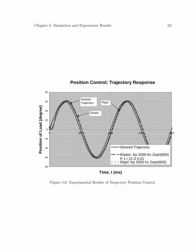
Chapter 5: Simulation and Experiment Results 62
Position Control: Trajectory Response
-80
-60
-40
-20
0
20
40
60
80
0 500 1000 1500 2000
Time, t (ms)
Po
siti
on
of
Lo
ad (
deg
ree)
Desired Trajectory
Elastic: Kp 2000 Kv 2sqrt(600) P 1 I 22 D 0.01Rigid: Kp 2000 Kv 2sqrt(600)
Desired Trajectory Rigid
Elastic
Figure 5.6: Experimental Results of Trajectory Position Control.
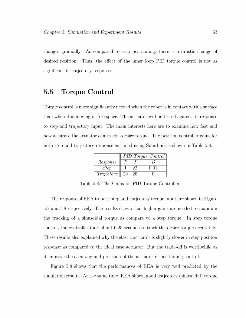
Chapter 5: Simulation and Experiment Results 63
changes gradually. As compared to step positioning, there is a drastic change of
desired position. Thus, the effect of the inner loop PID torque control is not as
significant in trajectory response.
5.5 Torque Control
Torque control is more significantly needed when the robot is in contact with a surface
than when it is moving in free space. The actuator will be tested against its response
to step and trajectory input. The main interests here are to examine how fast and
how accurate the actuator can track a desire torque. The position controller gains for
both step and trajectory response as tuned using SimuLink is shown in Table 5.8.
PID Torque ControlResponse P I D
Step 1 22 0.01Trajectory 20 20 0
Table 5.8: The Gains for PID Torque Controller.
The response of REA to both step and trajectory torque input are shown in Figure
5.7 and 5.8 respectively. The results shown that higher gains are needed to maintain
the tracking of a sinusoidal torque as compare to a step torque. In step torque
control, the controller took about 0.25 seconds to track the desire torque accurately.
These results also explained why the elastic actuator is slightly slower in step position
response as compared to the ideal case actuator. But the trade-off is worthwhile as
it improve the accuracy and precision of the actuator in positioning control.
Figure 5.8 shows that the performances of REA is very well predicted by the
simulation results. At the same time, REA shown good trajectory (sinusoidal) torque

Chapter 5: Simulation and Experiment Results 64
Torque Control : Step ResponseP 20 I 20 D 0.01
-1
0
1
2
3
4
5
6
0 0.1 0.2 0.3 0.4 0.5 0.6 0.7 0.8 0.9 1
Time, t (s)
Ou
tpu
t T
orq
ue,
TL
(N
M)
Desired TorqueSimulation Experiment
Desired Torque
SimulationExperiment
Figure 5.7: Torque Control: Step Response of REA.
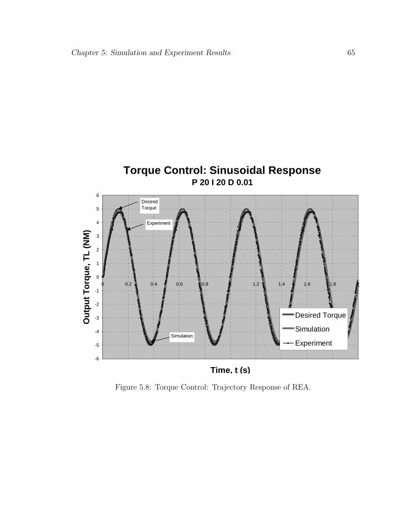
Chapter 5: Simulation and Experiment Results 65
Torque Control: Sinusoidal ResponseP 20 I 20 D 0.01
-6
-5
-4
-3
-2
-1
0
1
2
3
4
5
6
0 0.2 0.4 0.6 0.8 1 1.2 1.4 1.6 1.8 2
Time, t (s)
Ou
tpu
t T
orq
ue,
TL
(N
M)
Desired Torque
Simulation
Experiment
Desired Torque
Simulation
Experiment
Figure 5.8: Torque Control: Trajectory Response of REA.

Chapter 5: Simulation and Experiment Results 66
control.
5.6 Force Control
There are two types of force control used here. Namely, force control for contact start
and force control for moving to contact.
5.6.1 Contact Start
Start with Contact: Force vs. Time
-1
0
1
2
3
4
5
6
0 0.5 1 1.5 2 2.5 3
Time,t (s)
Fo
rce,
F (
N)
Elastic: Outer: P 1 I 10, Inner: P 1 I 22
Rigid 1 : P 1 I 10 D 0.03 Tsf 4 b 7
Rigid 2 : P 1 I 10
Desired Force
Rigid 2
Elastic
Rigid 1
Desired Force
Figure 5.9: Simulation Results of Force Control Start With Contact.
The gains of the controllers in Table 5.9 are selected arbitrarily for the purpose of
performance comparison between the actuators. This is to ensure that all actuators

Chapter 5: Simulation and Experiment Results 67
Start with Contact: Force vs. Time
-1
0
1
2
3
4
5
6
0 0.5 1 1.5 2 2.5 3
Time,t (s)
Fo
rce,
F (
N)
Elastic: Outer: P 1 I 10, Inner: P 1 I 22
Rigid 1 : P 1 I 10 D 0.03 Tsf 4 b 7
Rigid 2 : P 1 I 10
Desired Force
Rigid 2
Elastic
Rigid 1
Desired Force
Figure 5.10: Experimental Results of Force Control Start With Contact.
are performed under the same amount of effort of actuation, e.g. the maximum torque
are the same for all actuators. Thus, all the actuators will be controlled by the same
outer loop force control regardless of their performances.
The simulation experimental results of force control that start with contact are
shown in Figures 5.9 and 5.10 respectively. Due to the softness of the Elastic Flywheel,
the response of the REA shown a little bit of overshoot and “discontinuities” as
compared to its rigid counterpart. The experimental results seems to have some
steady state errors as compared to the simulation results. This is due the analog effect
of the load cell used in the experiment which introduced noise in to the feedback loop.
The response of Rigid 2 is about 0.4 seconds slower than the other two actuators.

Chapter 5: Simulation and Experiment Results 68
Outer Loop Inner Loop DynamicActuator Force Control Torq. Control Compensation
P I D P I D Tsf bRigid 1 1 10 0 0 0 0 4 7Rigid 2 1 10 0.08 0 0 0 0 0Elastic 1 10 0 1 22 0 0 0
Table 5.9: The Gains and Dynamic Compensation for Force Control.
This is mainly because the chosen Integral term used in the experiment is not fast
enough to compensate the frictions in the actuator. However, these frictions are well
compensated through the implementation of the inner loop torque control into REA.
Although the response of REA is slightly slower than Rigid 1 according to SimuLink.
But the real-life experiments showed that REA is as fast as Rigid 1 in force control.
In contrast to the simulation, perfect dynamic compensations are almost impossible
in the experiments. In simulations, only dynamic and static frictions are modelled
and compensated. On the other hand, there are also non-linearities such as coulomb
frictions and backlashes exist in the system. Thus, this is why Rigid 1 is slower in ex-
periment than what SimuLink predicted, where as REA can easily compensate these
frictions using inner loop torque control.
5.6.2 Moving to Contact
Force control by itself is found to be inadequate in condition where robots are initially
moving in free space and then come into contact with the environment. Thus, hybrid
speed/control is use to control the robots in both environments.
The gains of force control moving to contact are first simulated using SimuLink
for safety purpose. Then, an uniform set of the controller’s gains is selected for all the
actuators. Thus, it can be assumed that all the actuators are controlled by the same

Chapter 5: Simulation and Experiment Results 69
control system. By doing so, the performance of the actuators can be compared and
evaluated. Refer to Table 5.10 for the gains and dynamic compensation for Hybrid
Speed/Force Control.
Hybrid Inner Loop DynamicActuator Speed Force Torq. Control Compensation
KP KV P I D P I D Tsf bRigid 1 0 200 1 10 0 0 0 0 4 7Rigid 2 0 200 1 10 0.08 0 0 0 0 0Elastic 0 200 1 10 0 1 22 0 0 0
Table 5.10: The Gains and Dynamic Compensation for Hybrid Speed/Force Control.
Figure 5.11 shows the experimental results of the actuator under hybrid speed/force
control, where it needs to move a certain unknown distance, for example 30 degrees
before its end-effector touches the working surface. Figure 5.12 shows that the set-
tling time for Rigid 1 and Elastic are about the same, where as the settling time of
Rigid 2 is about 0.35 seconds slower than the previous two actuators.
Although the collision occurs severely between all the actuators and their working
surface. The reflected torque transmitted to the system are greatly reduced for REA
as the elastic flywheel somewhat low pass the reflected torque. From Figure 5.13,
it can be shown that the reflected torque of REA peak at 5Nm after more than 0.3
seconds, while the reflected torque for the rigid actuators can reach up to 50 Nm
instantaneously, namely in less than 1 miliseconds.
Furthermore, the rigid actuators exhibit great vibration and instability while per-
forming these tasks. To resolve this problem, the size of the gearbox used for the
rigid actuators need to be fairly big in order to withstand the high reflected torque.
However, big heavy-duty gearbox can over burden the system while still failed to
maintain the stability of the system. Thus, elasticity in the actuator is an ideal way
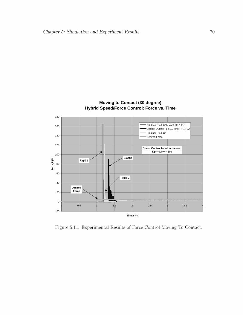
Chapter 5: Simulation and Experiment Results 70
Moving to Contact (30 degree)Hybrid Speed/Force Control: Force vs. Time
-20
0
20
40
60
80
100
120
140
160
180
0 0.5 1 1.5 2 2.5 3 3.5 4
Time,t (s)
Fo
rce,
F (
N)
Rigid 1 : P 1 I 10 D 0.03 Tsf 4 b 7
Elastic: Outer: P 1 I 10, Inner: P 1 I 22
Rigid 2 : P 1 I 10
Desired Force
Rigid 2
ElasticRigid 1
Desired Force
Speed Control for all actuators:Kp = 0, Kv = 200
Figure 5.11: Experimental Results of Force Control Moving To Contact.

Chapter 5: Simulation and Experiment Results 71
Moving to Contact (30 degree)Hybrid Speed/Force Control: Force vs. Time
0
2
4
6
8
10
12
14
16
18
20
0 0.5 1 1.5 2 2.5 3 3.5 4
Time,t (s)
Fo
rce,
F (
N)
Rigid 1 : P 1 I 10 D 0.03 Tsf 4 b 7
Elastic: Outer: P 1 I 10, Inner: P 1 I 22
Rigid 2 : P 1 I 10
Desired Force
Rigid 2
ElasticRigid 1
Desired Force
Speed Control for all actuators:Kp = 0, Kv = 200
Figure 5.12: Experimental Results of Force Control Moving To Contact (Magnified).
to maintain the stability and protect the system from damages as a consequence of
collision.

Chapter 5: Simulation and Experiment Results 72
Moving to Contact (30 degree)Hybrid Speed/Force Control:
Reflected Torque on Gear vs. Time
-60
-40
-20
0
20
40
60
0 0.2 0.4 0.6 0.8 1 1.2 1.4 1.6 1.8 2
Time,t (s)
To
rqu
e,T
rf (
Nm
)
Rigid 2 : P 1 I 10
Rigid 1 : P 1 I 10 D 0.03 Tsf 4 b 7
Elastic: Outer: P 1 I 10, Inner: P 1 I 22
Rigid 2
Elastic
Rigid 1
Speed Control for all actuators:Kp = 0, Kv = 200
Figure 5.13: Reflected Torque of Actuators.

Chapter 6
Conclusions
6.1 Summary of Work Done
For a typical robotic application, where frictions and non-linearities of motor drive
system are inherent, the performance can be improved by introducing an inner loop
torque controller into its original position controlled actuator. The main purpose of
the inner loop control is to account for the frictional loss and noises found in between
the motor source and the output load which affect the accuracy of the output position.
The inner loop control served the same purpose as incorporating the dynamics of the
actuator into its controller. However, the process of identifying the dynamics can be
very time-consuming and simply not possible in some existing system.
By using the Elastic Flywheel as part of the torque sensor, REA is also capable
of generating accurate torque. This feature is particularly essential for manipula-
tor when interacting with working surfaces under kinematic constraints. With the
presence of elasticity, the actuator becomes more shock tolerant and enable better in-
teraction between the robotic structure and its working surface. The elasticity in the
actuator which minimize the vibrations of the robotic system can improve stability
73

Chapter 6: Conclusions 74
of torque/force control. Some other added advantages of the elasticity such as lower
reflected inertia, better energy storage capacity and less inadvertent damage to the
environment are also very favorable in robotic application.
As far as the movements of animals are concerned, their contact with environment
are felt through a series of elastic tendons to maintain their stability in locomotion.
These tendons not only allow the animal to have immediate cognition in moving itself
in unknown environment but also its energy can be stored and released elastically.
Animals commonly utilize the elasticity of tendons to store energy from one part of a
locomotive cycle to release it in another. Since the muscles are doing less work overall
than it otherwise would be, this potentially improves efficiency. Thus, actuators with
series elasticity will allow the same effect to happen in robots, extending the life of
battery.
The Rotary Elastic Actuator have proven to boast the performance of the tradi-
tional position control methods, especially in cases where non-linearities are excessive
in the motor drive and transmission systems. At the same, the actuator is also capa-
ble of force/torque control, multi-revolution and its elastic nature have already shown
to contribute improvements and benefits in applications such as bipedal walking[1],
human-robots interactions [9] and other torque /force inherent tasks[5].
6.2 Future Work
Several avenues are open for future works. Although significant efforts have been put
in making the elastic flywheel to be a compact and yet modular one, its current size
can still be minimize. This has opened doors to future effort in reducing the size
of this elastic torque sensor. Some suggested ways of improvements are rearranging

Chapter 6: Conclusions 75
the springs diagonally or over-lapping the springs to achieve smaller diameter of the
elastic flywheel.
As far as the precision of the measurements of the deflection of the flywheel are
concerned, sensors e.g. encoders should be mounted as close as possible to the fly-
wheel. Since non-linearities such as backlash and friction are found in the gearbox
and couplings , this will contribute to the systematic errors. To minimize these er-
rors, one encoder should be installed in between the elastic flywheel to measure the
torsional deflection of the elastic flywheel and another encoder on the output of the
actuator to measure the actual output position of the actuator.

Bibliography
[1] Gill A. Pratt and Matthew M. Williamson. Series elastic actuator. The MIT
Press, Cambridge, MA., 2000.
[2] Et. Al. Gill A. Pratt, MAtthew M. Williamson. Stiffness isn’t everything. In
Proceedings of ISER. The MIT Press, 1995.
[3] David W. Robinson. Design and Analysis of series Elasticity in Closed-loop
Actuator Force Control. PhD thesis, MIT, June 2000.
[4] Garen Timonsheko. Mechanic of Materials. Wesley Press, 3 edition, 1998.
[5] Eppinger S. D. and Seering W. P. Three dynamic probelms in robot force control.
IEEE Intl Coonference on Robotics and Automation, 1989.
[6] Atkeson C. G. An H. C. and Holler J. M. Model based control of a robot
manipulator. MIT Press, Cambridge MA., 1988.
[7] Honda Robotic Group. Humanoid robots. http://www.world.honda.com/robot/,
November 2002.
[8] Roberts R. K. The compliance of end effector force sensors for robot manipulator
control. Master’s thesis, School of Electrical Engineering, Purdue Univ., 1992.
[9] Whitney D. E. Historical perspective and state of the art in robot force contro.
In Intl J. of Robotics Research, volume 6 of 1, Spring 1987.
76

[10] Mason M. T. and Lynch K. M. Dynamic manipulation. In Proceedings of the
IEEE/RSJ Intl Workshop on Intelligent Robots and Systems (IROS-93), pages
152–159. Yokohama, Japan, 1993.
[11] Salisbury J. K. Active stiffness control of a manipulator in cartesian coordi-
nates. 19th IEEE Conference on Decision and Control, pages 95–100, December
1990.
[12] Hogan N. Impedance control: An approach to manipulation: Part 1 - theory, part
2 - implementation, and part 3 - applications. ASME J. of Dynamic Systems,
Measurement and Control, pages 1–24, 1990.
[13] Raibert H. M. and Craig J. J. Hybrid position/force control of manipu- lators.
Trans ASME Journal of Dynamic Systems, Measurement and Control, 103:126–
133, June 1981.
[14] Cannon R. H. and Rosenthal D. E. Experiments in control of flexible struc-
tures with noncolocated sensors and actuators. AIAA Journal of Guidance and
Control, 3(3):546–553, Sept.-Oct. 1984.
[15] Xu Y. and Ma D. Force and transient control using nonlinear pd control. IEEE
Intl Conf on Robotics and Automation, pages 924–930, 1984.
[16] Wu C. H. and Paul R. Manipulator compliance based on joint torque con- trol.
Proc IEEE Conf on Decision and Control, Alberquerque, NM., pages 88–94, 1990.
[17] Tarn T. J. Marth G. T. and Bejczy A. K. An event based approach to impact
control: Theory and experiments. EEE Intl Conf on Robotics and Automation,
pages 918–923, 1994.
[18] Volpi R. and Khosla P. A theoretical and experimental investigation of ex-
plicit force control stategies for manipulators. IEEE Trans. Automatic Con-
trol, 38(11), November 1993.

[19] Yousef-Toumi K. and Gutz D. A. Impact and force control. IEEE Intl Conf on
Robotics and Automation, pages 410–416, 1989.
[20] Asada H. and Kanade T. Design of direct-drive mechanical arms. ASME Journal
of Vibration, Acoustics, Stress, and Reliability in Design, 105(3):312–316, 1992.
[21] Dieter Vischer and Khatib Oussama. Design and development of high perfor-
mance torque-controlled joints. IEEE Transactions on Robotics and Automa-
tions, 4(11):537–544, 1995.
[22] B. Tondu and P. Lopez. Modeling and control of mckibben artificial muscle robot
actuators. IEEE Control Systems Magazine, April 2000.
[23] John J Craig. Introduction to Robotics : Mechanics and Control. Addison-Wesley
Publishing Company, 2nd edition, 1989.
[24] Barnes Group. Catalogue of Stock Springs and Spring Washers, 2001.
[25] Servo To Go, Inc., 1716 221 place NE, Redmond, WA 98053. ISA Bus Servo I/O
Card Model 2 Hardware Manual., 2.0 edition, May 1999.
[26] Venture Com, Inc., Fice Cambridge Center, Cambridge MA 02142. RTX 5.0
User Manual, 1.0 edition, 2000.
[27] Khatib O. Jamisola R., Ang M. Jr. and Lim S. Y. Dynamics identification and
control of an industrial robot. Proceedings of the Ninth International Conference
on Advanced Robotics (ICAR’99), pages 323–328, October 1999.

Appendix A
Technical Drawings
79

A.1 Part List of Rotary Elastic Actuator (REA)
1
2
3
45
6
9
1011
7
8D E FC
12
34
BA
32
15
C D
46
78
A B
A4
SHEE
T 1
OF
1SC
ALE
:1:2
DW
G N
O.
TITL
E:NA
TIO
NA
L U
NIV
ERSI
TY O
F SI
NG
APO
RE
DO
NO
T SC
ALE
DRA
WIN
GW
EIG
HT:
MA
TERI
AL:
DA
TEN
AM
E
FIN
ISH
:
UN
LESS
OTH
ERW
ISE
SPEC
IFIE
D:
DIM
ENSI
ON
S A
RE IN
MIL
LIM
ETER
SSU
RFA
CE
FIN
ISH
:TO
LERA
NC
ES:
L
INEA
R:
�
� +/- 0
.1
AN
GU
LAR:
� +/- 0
.1M
FG
APP
V'D
CH
K'D
DRA
WN
PRO
PRIE
TARY
AN
D C
ON
FID
ENTI
AL
THE
INFO
RMA
TIO
N C
ON
TAIN
ED I
N T
HIS
DRA
WIN
G IS
TH
E SO
LE P
ORP
ERTY
OF
AD
ELA
IDE
UN
IVER
SITY
. AN
Y RE
PRO
DU
CTI
ON
IN P
ART
OR
AS
A W
HO
LE W
ITH
OU
TTH
E W
RITT
EN P
ERM
ISSI
ON
OF
AD
ELA
IDE
UN
IVER
SITY
IS P
ROH
IBIT
ED
EMC
HA
I22
/10/
'02
VA
RIES
VA
RIES
EM -
PL -
01
Part
List
1-
Ge
ne
ral
613.
9 G
M
Ite
m N
o:
De
sc
rip
tio
ns
:1
MO
TO
R E
NC
OD
ER
25
00
PP
R2
PA
NA
SO
NIC
40
0W
SE
RV
OM
OT
OR
34
0 :
1 G
EA
RB
OX
4M
OT
OR
BR
AC
KE
T5
CO
UP
LIN
G6
FL
EX
IBL
E F
LY
WH
EE
L7
BE
AR
ING
SU
PP
OR
T U
NIT
8D
UM
MY
WE
IGH
T
9E
NC
OD
ER
BR
AC
KE
T1
0B
EA
RIN
G U
NIT
11
OU
TP
UT
EN
CO
DE
R 2
50
0 P
PR
Figure A.1: Part List of Rotary Elastic Actuator.

A.2 Part List of Elastic Flywheel
13
14
11
15
1118
20
16
3
45
2
106
87
17
19
1
9
12
Ass
em
ble
d V
iew
Exp
lod
ed
Vie
w
D E FC
12
34
BA
32
15
C D
46
78
A B
A4
SHEE
T 1
OF
1SC
ALE
:1:2
DW
G N
O.
TITL
E:NA
TIO
NA
L U
NIV
ERSI
TY O
F SI
NG
APO
RE
DO
NO
T SC
ALE
DRA
WIN
GW
EIG
HT:
MA
TERI
AL:
DA
TEN
AM
E
FIN
ISH
:
UN
LESS
OTH
ERW
ISE
SPEC
IFIE
D:
DIM
ENSI
ON
S A
RE IN
MIL
LIM
ETER
SSU
RFA
CE
FIN
ISH
:TO
LERA
NC
ES:
L
INEA
R:
�
� +/- 0
.1
AN
GU
LAR:
� +/- 0
.1M
FG
APP
V'D
CH
K'D
DRA
WN
PRO
PRIE
TARY
AN
D C
ON
FID
ENTI
AL
THE
INFO
RMA
TIO
N C
ON
TAIN
ED I
N T
HIS
DRA
WIN
G IS
TH
E SO
LE P
ORP
ERTY
OF
AD
ELA
IDE
UN
IVER
SITY
. AN
Y RE
PRO
DU
CTI
ON
IN P
ART
OR
AS
A W
HO
LE W
ITH
OU
TTH
E W
RITT
EN P
ERM
ISSI
ON
OF
AD
ELA
IDE
UN
IVER
SITY
IS P
ROH
IBIT
ED
EMC
HA
I22
/10/
'02
VA
RIES
VA
RIES
EM -
PL -
02
Part
List
2 -
Fle
xib
le F
lyw
he
el
ITE
M N
O.
QTY
.P
AR
T N
O.
RE
FE
NC
E N
O.:
MA
TER
IAL
WE
IGH
T (G
M)
11
MID
DLE
SH
AF
TE
M-F
F-0
8S
tain
less
Ste
el38
3.67
212
M3
CA
P S
CR
EW
x 1
0 m
mS
002-
003-
010
Har
dene
d S
teel
33
1TH
RIS
T B
EA
RIN
G 1
5 TO
PG
S.8
1102
Har
dene
d S
teel
104
1TH
RU
ST
BE
AR
ING
15
BA
SE
WS
.811
02H
arde
ned
Ste
el10
51
THR
US
T B
EA
RIN
G 1
5 C
EN
TER
KS
.811
02LP
BH
arde
ned
Ste
el6
61
BA
LL B
EA
RIN
G
6180
0TH
igh
Str
engh
Ste
el5
71
M6
CA
P S
CR
EW
x 1
0 m
mS
022-
006-
010
Hig
h S
tren
gh S
teel
48
1M
6 W
AS
HE
RW
10-0
06-0
000
Hig
h S
tren
gh S
teel
19
1M
OTO
R H
UB
E
M-F
F-0
4S
tain
less
Ste
el13
5.86
101
CE
NTE
R
BE
AR
ING
HO
US
ING
E
M-F
F-0
2S
tain
less
Ste
el79
.31
118
SP
RIN
G S
LID
ER
E
M-F
F-1
4A
lum
inum
Allo
y12
.99
128
SP
RIN
G W
AS
HE
R
EM
-FF
-15
Sta
inle
ss S
teel
3.24
138
M5
PH
ILLI
P S
CR
EW
x 8
0 m
mP
10-0
05-0
80H
igh
Str
engh
Ste
el15
1416
M4
CS
K x
16
mm
S02
9-00
4-01
6H
igh
Str
engh
Ste
el4
1516
CE
RA
MIC
BU
SH
(D
ia.
5.5
mm
)P
AP
040
3 P
10S
tain
less
Ste
el1
1616
M3
SE
T S
CR
EW
x 4
mm
S30
-003
-004
Hig
h S
tren
gh S
teel
317
16E
XTE
NS
ION
SP
RIN
GT4
2690
Hig
h S
tren
gh S
teel
5018
1O
UTP
UT
FLY
WH
EE
L E
M-F
F-0
7A
lum
inum
Allo
y36
1.21
198
M4
CA
P S
CR
EW
x 1
6 m
mS
002-
004-
016
Hig
h S
tren
gh S
teel
420
1M
OTO
R F
LYW
HE
EL
EM
-FF
-05
Alu
min
umA
lloy
361.
21
Figure A.2: Part List of Elastic Flywheel.

A.3 Part Files

A.3.1 Center Bearing Housing
40
28
16
30
FRO
NT
VIE
W
4 H
OLE
S M
3 X
0.5
-6H
EQU
I-SPA
CED
ON
35
MM
4 H
OLE
S M
4 X
0.6
- 6H
EQU
I-SPA
CED
ON
30
MM
45°
ISO
MET
RIC
VIE
WSc
ale
1 :
1
13.5
0 65.
50
16
19
40
283
Q-Q
SE
CTI
ON
AL
VIE
W
B C D
12
A
32
14
BA
56
UN
LESS
OTH
ERW
ISE
SPEC
IFIE
D:
DIM
ENSI
ON
S A
RE
IN M
ILLI
MET
ERS
SUR
FAC
E FI
NIS
H: G
RA
DE
6TO
LER
AN
CES
:
LIN
EAR
:
+
/- 0
.1
AN
GU
LAR
:
+
/- 0
.1
FIN
ISH
:
NA
ME
DA
TE
MA
TER
IAL:
WEI
GH
T:
NA
TIO
NA
L U
NIV
ERSI
TY O
F SI
NG
APO
RETI
TLE:
DW
G N
O.
SCA
LE:2
:1SH
EET
1 O
F 1
A4C
Ce
nte
r Be
arin
g H
ous
ing
EM -
FF -
02
DR
AW
N
CH
K'D
DR
AW
N
MFG
AP
PV
'D
CH
K'D
PRO
PRIE
TARY
AN
D C
ON
FID
ENTI
AL
THE
INFO
RMA
TIO
N C
ON
TAIN
ED IN
TH
IS
DR
AW
ING
IS T
HE
SOLE
PRO
PERT
Y O
FA
DEL
AD
IE U
NIV
ERSI
TY. A
NY
REPR
OD
UC
TIO
N
IN P
ART
OR
AS
A W
HO
LE W
ITH
OU
T TH
E W
RIT
TEN
PER
MIS
SIO
N O
F A
DEL
AID
EU
NIV
ERSI
TY IS
PRO
HIB
ITED
.
STA
INLE
SS S
TEEL
MIL
LEMC
HA
I19
/10/
'02
DO
NO
T SC
ALE
DRA
WIN
G77
.54
GM
Figure A.3: Center Bearing Housing.

A.3.2 Motor Hub
40
20
C C
4 H
OLE
S M
4 X
0.7
- 6H
EQU
I-SPA
CED
ON
30
FRO
NT
VIE
W
30
4
40
1215
19R1
3 5
R1
C-C
SEC
TIO
NA
L V
IEW
ISO
MET
RIC
VIE
WSC
ALE
: 1:
1
135.
85 G
M
B C D
12
A
32
14
BA
56
UN
LESS
OTH
ERW
ISE
SPEC
IFIE
D:
DIM
ENSI
ON
S A
RE
IN M
ILLI
MET
ERS
SUR
FAC
E FI
NIS
H: G
RA
DE
6TO
LER
AN
CES
:
LIN
EAR
:
+
/- 0
.1
AN
GU
LAR
:
+
/- 0
.1
FIN
ISH
:
NA
ME
DA
TE
MA
TER
IAL:
WEI
GH
T:
NA
TIO
NA
L U
NIV
ERSI
TY O
F SI
NG
APO
RETI
TLE:
DW
G N
O.
SCA
LE:2
:1SH
EET
1 O
F 1
A4C
Mo
tor H
ub
EM
-FF-
04
DR
AW
N
CH
K'D
DR
AW
N
MFG
AP
PV
'D
CH
K'D
PRO
PRIE
TARY
AN
D C
ON
FID
ENTI
AL
THE
INFO
RMA
TIO
N C
ON
TAIN
ED IN
TH
IS
DR
AW
ING
IS T
HE
SOLE
PRO
PERT
Y O
FA
DEL
AD
IE U
NIV
ERSI
TY. A
NY
REPR
OD
UC
TIO
N
IN P
ART
OR
AS
A W
HO
LE W
ITH
OU
T TH
E W
RIT
TEN
PER
MIS
SIO
N O
F A
DEL
AID
EU
NIV
ERSI
TY IS
PRO
HIB
ITED
.
STA
INLE
SS S
TEEL
TURN
ING
EMC
HA
I27
/09/
'01
DO
NO
T SC
ALE
DRA
WIN
G
Figure A.4: Motor Hub.

A.3.3 Motor Flywheel
24
4
2022
SID
E V
IEW
200
R90
76
4025
20
EQU
I-SPA
CED
ON
30
4 H
OLE
S 4
74
EQU
I-SPA
CED
O
N R
97
8 H
OLE
S 2
1020
22
4 H
OLE
S 7
X 2
MM
DEE
P EQ
UI-S
PAC
ED
ABO
UT
CEN
TERL
INE
4 W
EBS
X 4M
M T
HK
CEN
TERE
D
8 H
OLE
S 20
4 H
OLE
S 50
90 A
PART
A
BOU
T C
ENTE
RLIN
E
FRO
NT
VIE
W
R97
30
45°
22.5
0°
ISO
MET
RIC
VIE
WSC
ALE
: 1:
4
B C D
12
A
32
14
BA
56
UN
LESS
OTH
ERW
ISE
SPEC
IFIE
D:
DIM
ENSI
ON
S A
RE
IN M
ILLI
MET
ERS
SUR
FAC
E FI
NIS
H: G
RA
DE
6TO
LER
AN
CES
:
LIN
EAR
:
+
/- 0
.1
AN
GU
LAR
:
+
/- 0
.1
FIN
ISH
:
NA
ME
DA
TE
MA
TER
IAL:
WEI
GH
T:
NA
TIO
NA
L U
NIV
ERSI
TY O
F SI
NG
APO
RE
TITL
E:
DW
G N
O.
SCA
LE:1
:2SH
EET
1 O
F 1
A4C
Mo
tor F
lyw
hee
l
EM -
FF -
05
DR
AW
N
CH
K'D
DR
AW
N
MFG
AP
PV
'D
CH
K'D
PRO
PRIE
TARY
AN
D C
ON
FID
ENTI
AL
THE
INFO
RMA
TIO
N C
ON
TAIN
ED IN
TH
IS
DR
AW
ING
IS T
HE
SOLE
PRO
PERT
Y O
FA
DEL
AD
IE U
NIV
ERSI
TY. A
NY
REPR
OD
UC
TIO
N
IN P
ART
OR
AS
A W
HO
LE W
ITH
OU
T TH
E W
RIT
TEN
PER
MIS
SIO
N O
F A
DEL
AID
EU
NIV
ERSI
TY IS
PRO
HIB
ITED
.
ALU
MIN
UM
ALL
OY
MIL
LEMC
HA
I27
/09/
'01
DO
NO
T SC
ALE
DRA
WIN
G34
9.95
GM
PRO
J.:
Figure A.5: Motor Flywheel.

A.3.4 Output Flywheel
2
4
4
2022
SID
E V
IEW
EQU
I-SPA
CED
ON
304
HO
LES
4R
3.50
4
20
2540
76
200
R90
1020
22
FRO
NT
VIE
W
4 W
EBS
X 4M
M T
HK
CEN
TERE
D
4 H
OLE
S 7
X 2M
M D
EEP
EQU
I-SPA
CED
A
BOU
T C
ENTE
RLIN
E
8 H
OLE
S 20
4 H
OLE
S 50
90 A
PART
ABO
UT
CEN
TERL
INE
R97
22.50°
45°
ISO
MET
RIC
VIE
WSC
ALE
: 1:
4
B C D
12
A
32
14
BA
56
UN
LESS
OTH
ERW
ISE
SPEC
IFIE
D:
DIM
ENSI
ON
S A
RE
IN M
ILLI
MET
ERS
SUR
FAC
E FI
NIS
H: G
RA
DE
6TO
LER
AN
CES
:
LIN
EAR
:
+
/- 0
.1
AN
GU
LAR
:
+
/- 0
.1
FIN
ISH
:
NA
ME
DA
TE
MA
TER
IAL:
WEI
GH
T:
NA
TIO
NA
L U
NIV
ERSI
TY O
F SI
NG
APO
RE
TITL
E:
DW
G N
O.
SCA
LE:1
:2SH
EET
1 O
F 1
A4C
OU
TPU
T FL
YWH
EEL
EM -
FF -
07
DR
AW
N
CH
K'D
DR
AW
N
MFG
AP
PV
'D
CH
K'D
PRO
PRIE
TARY
AN
D C
ON
FID
ENTI
AL
THE
INFO
RMA
TIO
N C
ON
TAIN
ED IN
TH
IS
DR
AW
ING
IS T
HE
SOLE
PRO
PERT
Y O
FA
DEL
AD
IE U
NIV
ERSI
TY. A
NY
REPR
OD
UC
TIO
N
IN P
ART
OR
AS
A W
HO
LE W
ITH
OU
T TH
E W
RIT
TEN
PER
MIS
SIO
N O
F A
DEL
AID
EU
NIV
ERSI
TY IS
PRO
HIB
ITED
.
ALU
MIN
UM
ALL
OY
MIL
LEMC
HA
I27
/09/
'01
DO
NO
T SC
ALE
DRA
WIN
G34
7.18
GM
PRO
J.:
Figure A.6: Output Flywheel.

A.3.5 Middle Shaft
Q Q
FRO
NT
VIE
W
8 H
ole
s M
3 X
0.5
ON
35
MM
TH
REA
DED
TH
RU
4 H
OLE
S M
4 X
0.7
ON
30
MM
THRE
AD
ED T
HRU
TOP
VIE
W
FRO
NT
VIE
W
ISO
MET
RIC
VIE
WSc
ale
: 1:
2
20°
20°
21°
21° 30 35
10
55
6
10
7.50
Q-Q
SEC
TIO
NA
L V
IEWM
6 H
OLE
MIN
. 18
MM
DEE
P
10
MM
HO
LEM
IN. 1
8 M
M D
EEP
2 H
OLE
S M
4 X
0.70
90 A
PART
THRE
AD
ED T
HRU
1013
15
4024
7815
8
6
R3R3
20
B C D
12
A
32
14
BA
56
UN
LESS
OTH
ERW
ISE
SPEC
IFIE
D:
DIM
ENSI
ON
S A
RE
IN M
ILLI
MET
ERS
SUR
FAC
E FI
NIS
H: G
RA
DE
6TO
LER
AN
CES
:
LIN
EAR
:
+
/- 0
.1
AN
GU
LAR
:
+
/- 0
.1
FIN
ISH
:
NA
ME
DA
TE
MA
TER
IAL:
WEI
GH
T:
Na
tion
al U
niv
ers
ity o
f Sin
ga
po
re
TITL
E:
DW
G N
O.
SCA
LE:1
:1SH
EET
1 O
F 1
A4C
MID
DLE
SH
AFT
EM -
FF -
08v2
DR
AW
N
CH
K'D
DR
AW
N
MFG
AP
PV
'D
CH
K'D
PRO
PRIE
TARY
AN
D C
ON
FID
ENTI
AL
THE
INFO
RMA
TIO
N C
ON
TAIN
ED IN
TH
IS
DR
AW
ING
IS T
HE
SOLE
PRO
PERT
Y O
FA
DEL
AD
IE U
NIV
ERSI
TY. A
NY
REPR
OD
UC
TIO
N
IN P
ART
OR
AS
A W
HO
LE W
ITH
OU
T TH
E W
RIT
TEN
PER
MIS
SIO
N O
F A
DEL
AID
EU
NIV
ERSI
TY IS
PRO
HIB
ITED
.
STA
INLE
SS S
TEEL
TURN
EMC
HA
I19
/10/
'02
DO
NO
T SC
ALE
DRA
WIN
G38
9.5
GM
Figure A.7: Middle Shaft.

A.3.6 Spring Slider
22
6
6
145 2
FRO
NT
VIE
W
M5
X 0.
8 - 6
HTH
REA
DED
TH
RU
2 H
OLE
S M
3 X
0.5
- 6H
THRE
AD
ED T
HRU
7
6
5
TOP
VIE
W
10
16.5
0
4
4
SID
E V
IEW
2 H
OLE
S M
4 X
0.7
-6H
MIN
. 10M
M T
HRE
AD
ED
ISO
MET
RIC
VIE
W
B C D
12
A
32
14
BA
56
UN
LESS
OTH
ERW
ISE
SPEC
IFIE
D:
DIM
ENSI
ON
S A
RE
IN M
ILLI
MET
ERS
SUR
FAC
E FI
NIS
H: G
RA
DE
6TO
LER
AN
CES
:
LIN
EAR
:
+
/- 0
.1
AN
GU
LAR
:
+
/- 0
.1
FIN
ISH
:
NA
ME
DA
TE
MA
TER
IAL:
WEI
GH
T:
NA
TIO
NA
L U
NIV
ERSI
TY O
F SI
NG
APO
RETI
TLE:
DW
G N
O.
SCA
LE:2
:1SH
EET
1 O
F 1
A4C
SPRI
NG
SLI
DER
EM -
FF -
09
DR
AW
N
CH
K'D
DR
AW
N
MFG
AP
PV
'D
CH
K'D
PRO
PRIE
TARY
AN
D C
ON
FID
ENTI
AL
THE
INFO
RMA
TIO
N C
ON
TAIN
ED IN
TH
IS
DR
AW
ING
IS T
HE
SOLE
PRO
PERT
Y O
FA
DEL
AD
IE U
NIV
ERSI
TY. A
NY
REPR
OD
UC
TIO
N
IN P
ART
OR
AS
A W
HO
LE W
ITH
OU
T TH
E W
RIT
TEN
PER
MIS
SIO
N O
F A
DEL
AID
EU
NIV
ERSI
TY IS
PRO
HIB
ITED
.
ALU
MIN
UM
ALL
OY
TURN
EMC
HA
I27
/09/
'01
DO
NO
T SC
ALE
DRA
WIN
G12
.80
GM
Figure A.8: Spring Slider.

A.3.7 Dummy Weight - Main
150
200
3 H
OLE
S 12
1812
35
40
40
FRO
NT
VIE
W
2040
35
20
5
ALL
CO
RNER
SR1
0
TOP
VIE
W
SID
E V
IEW
ISO
MET
RIC
VIE
W
B C D
12
A
32
14
BA
56
UN
LESS
OTH
ERW
ISE
SPEC
IFIE
D:
DIM
ENSI
ON
S A
RE
IN M
ILLI
MET
ERS
SUR
FAC
E FI
NIS
H: G
RA
DE
6TO
LER
AN
CES
:
LIN
EAR
:
+
/- 0
.1
AN
GU
LAR
:
+
/- 0
.1
FIN
ISH
:
NA
ME
DA
TE
MA
TER
IAL:
WEI
GH
T:
NA
TIO
NA
L U
NIV
ERSI
TY O
F SI
NG
APO
RE
TITL
E:
DW
G N
O.
SCA
LE:1
:3SH
EET
1 O
F 1
A4C
Dum
my
We
ight
- M
ain
EM -
FF -
10
DR
AW
N
CH
K'D
DR
AW
N
MFG
AP
PV
'D
CH
K'D
PRO
PRIE
TARY
AN
D C
ON
FID
ENTI
AL
THE
INFO
RMA
TIO
N C
ON
TAIN
ED IN
TH
IS
DR
AW
ING
IS T
HE
SOLE
PRO
PERT
Y O
FA
DEL
AD
IE U
NIV
ERSI
TY. A
NY
REPR
OD
UC
TIO
N
IN P
ART
OR
AS
A W
HO
LE W
ITH
OU
T TH
E W
RIT
TEN
PER
MIS
SIO
N O
F A
DEL
AID
EU
NIV
ERSI
TY IS
PRO
HIB
ITED
.
CO
PPER
MIL
LEMC
HA
I27
/09/
'01
DO
NO
T SC
ALE
DRA
WIN
G13
.77
KG
Figure A.9: Dummy Weight - Main.

A.3.8 Dummy Weight - Level
HO
LE
20R2
0
11.6
0
6
30
35
20
11 H
OLE
S12
FRO
NT
VIE
W
40
2 H
OLE
S M
6 X
1 - 6
H90
APA
RT A
BOU
T C
ENTE
RLIN
ETH
REA
DED
TH
RU
TOP
VIE
W
280
2010
SID
E V
IEW
ISO
MET
RIC
VIE
W
SCA
LE :
1:2
466.
91 G
M
B C D
12
A
32
14
BA
56
UN
LESS
OTH
ERW
ISE
SPEC
IFIE
D:
DIM
ENSI
ON
S A
RE
IN M
ILLI
MET
ERS
SUR
FAC
E FI
NIS
H: G
RA
DE
6TO
LER
AN
CES
:
LIN
EAR
:
+
/- 0
.1
AN
GU
LAR
:
+
/- 0
.1
FIN
ISH
:
NA
ME
DA
TE
MA
TER
IAL:
WEI
GH
T:
NA
TIO
NA
L U
NIV
ERSI
TY O
F SI
NG
APO
RETI
TLE:
DW
G N
O.
SCA
LE:1
:3SH
EET
1 O
F 1
A4C
Dum
my
We
ight
- Le
vel
EM -
FF -
12
DR
AW
N
CH
K'D
DR
AW
N
MFG
AP
PV
'D
CH
K'D
PRO
PRIE
TARY
AN
D C
ON
FID
ENTI
AL
THE
INFO
RMA
TIO
N C
ON
TAIN
ED IN
TH
IS
DR
AW
ING
IS T
HE
SOLE
PRO
PERT
Y O
FA
DEL
AD
IE U
NIV
ERSI
TY. A
NY
REPR
OD
UC
TIO
N
IN P
ART
OR
AS
A W
HO
LE W
ITH
OU
T TH
E W
RIT
TEN
PER
MIS
SIO
N O
F A
DEL
AID
EU
NIV
ERSI
TY IS
PRO
HIB
ITED
.
ALU
MIN
UM
ALL
OY
MIL
LEMC
HA
I27
/09/
'01
Figure A.10: Dummy Weight - Main.

A.3.9 Dummy Weight - Bolt
40 205
FRO
NT
VIE
W
35 40
40 35
TOP
VIE
W
3 H
OLE
S M
12 X
1.2
5TH
REA
DED
TH
RU
25
150
2 X
R10
SID
E V
IEW
ISO
MET
RIC
VIE
W
1.12
KG
B C D
12
A
32
14
BA
56
UN
LESS
OTH
ERW
ISE
SPEC
IFIE
D:
DIM
ENSI
ON
S A
RE
IN M
ILLI
MET
ERS
SUR
FAC
E FI
NIS
H: G
RA
DE
6TO
LER
AN
CES
:
LIN
EAR
:
+
/- 0
.1
AN
GU
LAR
:
+
/- 0
.1
FIN
ISH
:
NA
ME
DA
TE
MA
TER
IAL:
WEI
GH
T:
NA
TIO
NA
L U
NIV
ERSI
TY O
F SI
NG
APO
RETI
TLE:
DW
G N
O.
SCA
LE:1
:2SH
EET
1 O
F 1
A4C
Dum
my
We
ight
- Bo
lt
EM -
FF -
11
DR
AW
N
CH
K'D
DR
AW
N
MFG
AP
PV
'D
CH
K'D
PRO
PRIE
TARY
AN
D C
ON
FID
ENTI
AL
THE
INFO
RMA
TIO
N C
ON
TAIN
ED IN
TH
IS
DR
AW
ING
IS T
HE
SOLE
PRO
PERT
Y O
FA
DEL
AD
IE U
NIV
ERSI
TY. A
NY
REPR
OD
UC
TIO
N
IN P
ART
OR
AS
A W
HO
LE W
ITH
OU
T TH
E W
RIT
TEN
PER
MIS
SIO
N O
F A
DEL
AID
EU
NIV
ERSI
TY IS
PRO
HIB
ITED
.
CO
PPER
MIL
LEMC
HA
I27
/09/
'01
Figure A.11: Dummy Weight - Bolt.

A.3.10 Slider Washer
514
4
10
2 X
R2 4
24
2
TOP
VIE
W
FRO
NT
VIE
W
TOP
VIE
W
ISO
MET
RIC
VIE
WSc
ale
: 3:
1
B C D
12
A
32
14
BA
56
UN
LESS
OTH
ERW
ISE
SPEC
IFIE
D:
DIM
ENSI
ON
S A
RE
IN M
ILLI
MET
ERS
SUR
FAC
E FI
NIS
H: G
RA
DE
6TO
LER
AN
CES
:
LIN
EAR
:
+
/- 0
.1
AN
GU
LAR
:
+
/- 0
.1
FIN
ISH
:
NA
ME
DA
TE
MA
TER
IAL:
WEI
GH
T:
NA
TIO
NA
L U
NIV
ERIS
TY O
F SI
NG
AP
OR
ETI
TLE:
DW
G N
O.
SCA
LE:5
:1SH
EET
1 O
F 1
A4C
Slid
er W
ash
er
EM -
FF -
14
DR
AW
N
CH
K'D
DR
AW
N
MFG
AP
PV
'D
CH
K'D
PRO
PRIE
TARY
AN
D C
ON
FID
ENTI
AL
THE
INFO
RMA
TIO
N C
ON
TAIN
ED IN
TH
IS
DR
AW
ING
IS T
HE
SOLE
PRO
PERT
Y O
FA
DEL
AD
IE U
NIV
ERSI
TY. A
NY
REPR
OD
UC
TIO
N
IN P
ART
OR
AS
A W
HO
LE W
ITH
OU
T TH
E W
RIT
TEN
PER
MIS
SIO
N O
F A
DEL
AID
EU
NIV
ERSI
TY IS
PRO
HIB
ITED
.
ALU
MIN
UM
ALL
OY
MIL
LEMC
HA
I10
/01/
'02
2.28
GM
Figure A.12: Slider Washer.

A.3.11 Motor Bracket
13
120
13
THR
U4
HO
LES
M8
X 1
.5 -
6H
99
9.50
17
13
120 60
30
FRO
NT
VIE
W
ISO
MET
RIC
VIE
W
TOP
VIE
W
70 H
OLE
EQU
I-SPA
CED
ON
10
04
HO
LES
M6
X1.
0 -
6H
112
9949
.50
49.5
0R10
SID
E V
IEW
D E FC
12
34
BA
32
15
C D
46
78
A B
A4
SHEE
T 1
OF
1SC
ALE
:1:2
DW
G N
O.
TITL
E:NA
TIO
NA
L U
NIV
ERSI
TY O
F SI
NG
APO
RE
DO
NO
T SC
ALE
DRA
WIN
GW
EIG
HT:
MA
TERI
AL:
DA
TEN
AM
E
FIN
ISH
:
UN
LESS
OTH
ERW
ISE
SPEC
IFIE
D:
DIM
ENSI
ON
S A
RE IN
MIL
LIM
ETER
SSU
RFA
CE
FIN
ISH
:TO
LERA
NC
ES:
L
INEA
R:
�
� +/- 0
.1
AN
GU
LAR:
� +/- 0
.1M
FG
APP
V'D
CH
K'D
DRA
WN
PRO
PRIE
TARY
AN
D C
ON
FID
ENTI
AL
THE
INFO
RMA
TIO
N C
ON
TAIN
ED I
N T
HIS
DRA
WIN
G IS
TH
E SO
LE P
ORP
ERTY
OF
AD
ELA
IDE
UN
IVER
SITY
. AN
Y RE
PRO
DU
CTI
ON
IN P
ART
OR
AS
A W
HO
LE W
ITH
OU
TTH
E W
RITT
EN P
ERM
ISSI
ON
OF
AD
ELA
IDE
UN
IVER
SITY
IS P
ROH
IBIT
ED
EMC
HA
I22
/05/
'02
ALU
MIN
UM
ALL
OY
MIL
LEM
- FF
- 20
MO
TOR
BR
AC
KET
613.
9 G
M
Figure A.13: Motor Bracket.

Appendix B
Controller Code Part I -
Calibration and Position Control
B.1 Calibration
94

B.1.1 Calibration - Header File
// MOTORCNTLRTX.H #define PI 3.14159265359 #define Jl 0.0149 //Inertia #define Js 0.0676 #define Jb1 0.2646 #define F0 43.3 //Initial force for spring #define Kp 60.0 #define Kv (2*sqrt(0.0)) #define fr 0.092 double t= 7.0; //ff double R =94.0; #define KS 760 #define alp atan(t/R) #defineK 10.4 #define Kc 240 #define L0 53.8 #define Lr 55*PI/180 //************** ServoToGo ************************************** #define STG_A 0x240 //ServoToGo Card A base address #define STGOff 0x400 //offset for high address space #define DAC0 0x250 #define pSharedMemory "SharedMemory" typedef struct Data { int handshake; BOOL startrtss; BOOL killRT; } DATASTRUCT; DATASTRUCT *pdata;
Figure B.1: Calibration - Header File.

B.1.2 Calibration - Main File
//CALIBRATION : SPRING'S STIFFNESS TEST. //By: Eddie Chai //Main File #include "stdafx.h" #include <iostream.h> #include <windows.h> #include <stdio.h> #include <conio.h> #include <stdlib.h> #include <fstream.h> #include <math.h> #include <rtapi.h> #include "motorcntlrtx.h" double f1[200000]; double f2[200000]; double dt[200000]; double c1[200000]; double c2[200000]; double Tc[200000]; double V[200000]; double M [200000]; double L [200000]; double Md [200000]; double Mdd [200000]; double Ld [200000]; double Ldd [200000]; double TS[200000]; int d = 20; // delay int p = 1 ; // interval time int i = 1; int v= 1; int runtime =200000/p; //100 of interval int n=0; double voltage; double interval = 0.001*p*d; //interval time BOOL flag=TRUE; BOOL start=TRUE; void Analog_Out (int channel, double voltage)
Figure B.2: Calibration - Main File Page 1.

{ //check voltage double t_voltage=0.0; int dig; if (voltage >10.0) t_voltage = 10.0; else if (voltage < -10.0) t_voltage = -10.0; else t_voltage = voltage; //t_voltage = -t_voltage; dig = (int)(8191 * (t_voltage+10)/20.0); //write to DAC Channel RtWritePortUshort( (PUSHORT) (DAC0), (USHORT)dig); } //Initialise encoders(pg27). void RltZeroCntr(int channel) { // int offset; PUCHAR addresspuc, addresspuc1; addresspuc = (PUCHAR)(STG_A + channel*2); //select CNTi.C RtWritePortUchar(addresspuc, (UCHAR)0x20); //Master Control Register. MRST master reset RtWritePortUchar(addresspuc, (UCHAR)0x68); //Input Control Register. RtWritePortUchar(addresspuc, (UCHAR)0x80); //Output Control Register. RtWritePortUchar(addresspuc, (UCHAR)0xc3); //Quadrature Register 4x quadrature mode RtWritePortUchar(addresspuc, (UCHAR)0x04); //Reset encoder counters to zero. addresspuc1=(PUCHAR)(STG_A+ 0x400 + 0x0e); //TMRCMD RtWritePortUchar(addresspuc1, (UCHAR)0x3a); //chose timer 0 RtWritePortUchar(addresspuc1, (UCHAR)0x7a); //chose timer 1 RtWritePortUchar(addresspuc1, (UCHAR)0xba); //chose timer 2 printf("ENCODER %d Initialization COMPLETE\n",channel); return; } //Read encoder counter i. Return counter reading value long RltReadCntr(int channel) { PUCHAR addresspuc, addresspuc1; UCHAR cntl; UCHAR cntm; UCHAR cnth; long cntr;
Figure B.3: Calibration - Main File Page 2.
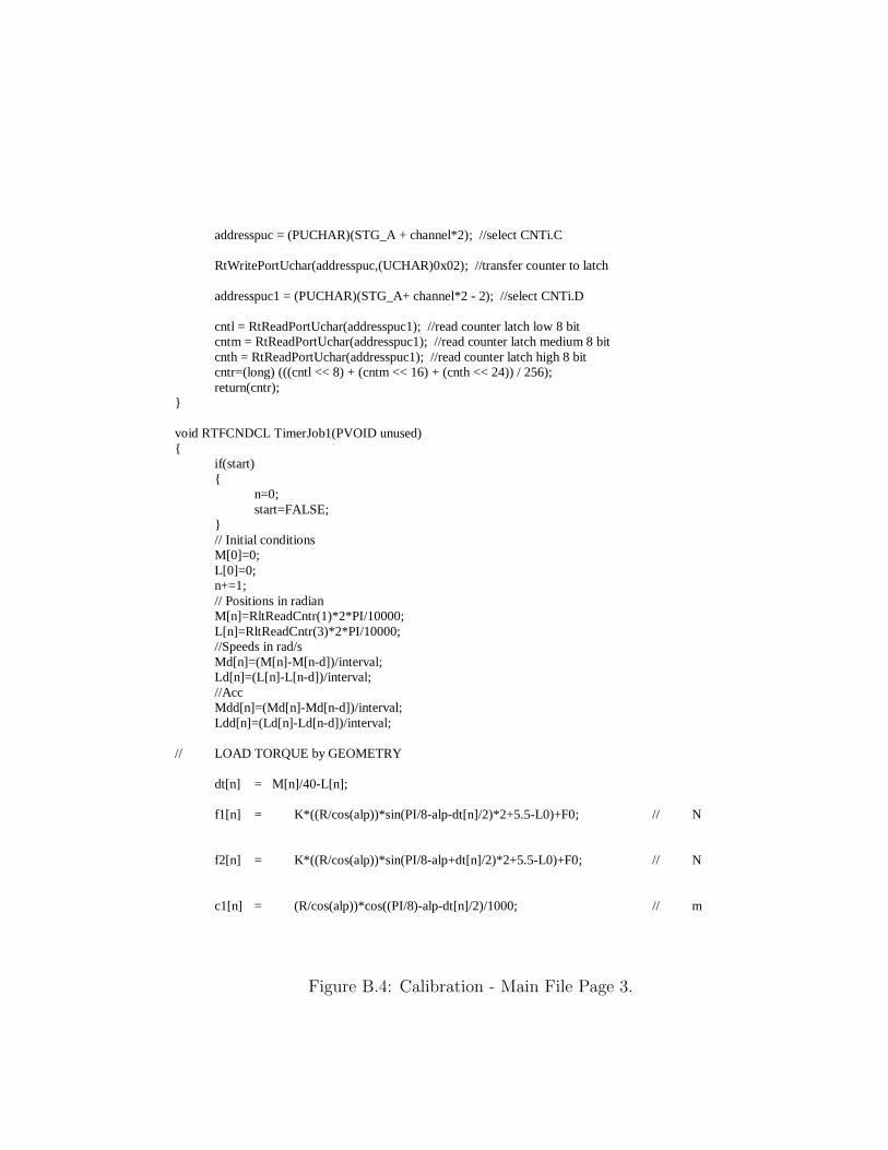
addresspuc = (PUCHAR)(STG_A + channel*2); //select CNTi.C RtWritePortUchar(addresspuc,(UCHAR)0x02); //transfer counter to latch addresspuc1 = (PUCHAR)(STG_A+ channel*2 - 2); //select CNTi.D cntl = RtReadPortUchar(addresspuc1); //read counter latch low 8 bit cntm = RtReadPortUchar(addresspuc1); //read counter latch medium 8 bit cnth = RtReadPortUchar(addresspuc1); //read counter latch high 8 bit cntr=(long) (((cntl << 8) + (cntm << 16) + (cnth << 24)) / 256); return(cntr); } void RTFCNDCL TimerJob1(PVOID unused) { if(start) { n=0; start=FALSE; } // Initial conditions M[0]=0; L[0]=0; n+=1; // Positions in radian M[n]=RltReadCntr(1)*2*PI/10000; L[n]=RltReadCntr(3)*2*PI/10000; //Speeds in rad/s Md[n]=(M[n]-M[n-d])/interval; Ld[n]=(L[n]-L[n-d])/interval; //Acc Mdd[n]=(Md[n]-Md[n-d])/interval; Ldd[n]=(Ld[n]-Ld[n-d])/interval; // LOAD TORQUE by GEOMETRY dt[n] = M[n]/40-L[n]; f1[n] = K*((R/cos(alp))*sin(PI/8-alp-dt[n]/2)*2+5.5-L0)+F0; // N f2[n] = K*((R/cos(alp))*sin(PI/8-alp+dt[n]/2)*2+5.5-L0)+F0; // N c1[n] = (R/cos(alp))*cos((PI/8)-alp-dt[n]/2)/1000; // m
Figure B.4: Calibration - Main File Page 3.

c2[n] = (R/cos(alp))*cos((PI/8)-alp+dt[n]/2)/1000; // m Tc[n] = 4*(f2[n]*c2[n]-f1[n]*c1[n]);// Nm // Load Torque assume linear relationship: TS[n] = dt[n]*KS; Analog_Out(0,0); if (n>= runtime) flag=FALSE; } int main() { LARGE_INTEGER x; LARGE_INTEGER Period; HANDLE hTimer; // HANDLE hToSharedMemory; RltZeroCntr(1); RltZeroCntr(3); printf("\n\nPlz Wait...\n"); Period.QuadPart=10000*p; if (!(hTimer = RtCreateTimer(NULL,0,TimerJob1,NULL,RT_PRIORITY_MAX,CLOCK_FASTEST))) // Always use fastest available clock { printf("SHUTDOWN: ERROR: Could not create the timer.\n"); ExitProcess(1); } if (!RtSetTimerRelative( hTimer, &Period, &Period)) { printf("SHUTDOWN: ERROR: Could not set and start the timer.\n"); ExitProcess(1); } printf("Kspring = %2.2fNm/rad\n",K); printf("Rspring = %3.1fmm\n",R); printf("sampling time = %3.1dms\n",p); printf("t(ms)\tM\t\tL\t\tdt\t\tMd(rpm)\tLd\t\tTs\n"); while(flag) {
Figure B.5: Calibration - Main File Page 4.
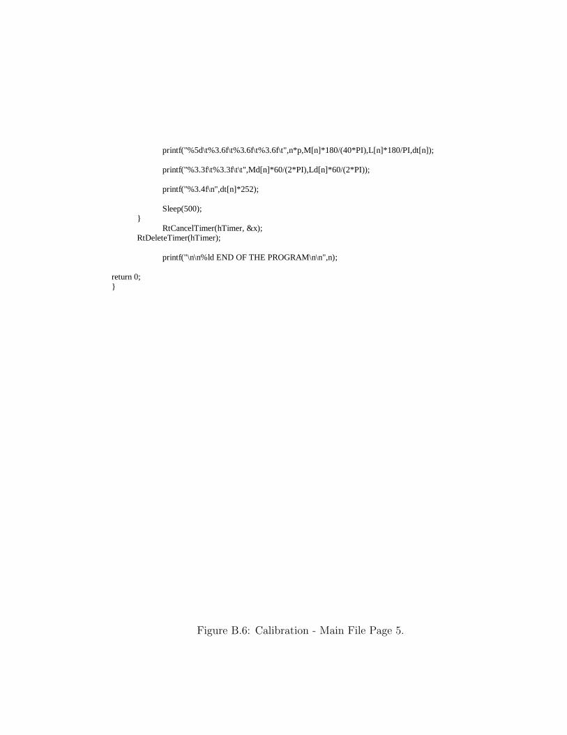
printf("%5d\t%3.6f\t%3.6f\t%3.6f\t",n*p,M[n]*180/(40*PI),L[n]*180/PI,dt[n]); printf("%3.3f\t%3.3f\t\t",Md[n]*60/(2*PI),Ld[n]*60/(2*PI)); printf("%3.4f\n",dt[n]*252); Sleep(500); } RtCancelTimer(hTimer, &x); RtDeleteTimer(hTimer); printf("\n\n%ld END OF THE PROGRAM\n\n",n); return 0; }
Figure B.6: Calibration - Main File Page 5.

B.2 Position Control

B.2.1 Position Control - Header File // POSITION CONTROL FOR STEP AND SINUSOIDAL INPUT // By: Eddie Chai // Header File // Control Architecture // Tm = [PID]*(Tl-Td) , where Tl = Ks(M-L) // Dynamics of Actuator // Tm = Tl + frictions // Tl = m*g*l*sin(L) + m*l^2*Ldd // Inertia term of Load, m*l^2 (kgm^2) #define Jl 0.0149 // lever only #define Js 0.0676 // small weight + lever // Gravitational term of Load, m*g*l (kgm^2s^-2 or N ) #define Gs 2.854 // small weight + lever // Coupling Parameters #define Kc 16.718 // Stiffness (Nm/deg) #define KS 426.0 // Overall Stiffness of Elastic Flywheel (Nm/rad) #define PI 3.14159265359 // Control Gains #define Kp 110 #define Kv 2*sqrt(110) #define P 1.0 #define I 22.0 #define D 0.0 // Desired Torque #define desire PI/3 // step //#define desire 20*sin((2*PI)*n/500) // Sinusoidal // Friction compensation #define fr 0.0 // Static/holding torque (% of Tm,max) //************** ServoToGo ************************************** #define STG_A 0x240 // ServoToGo Card A base address #define STGOff 0x400 // offset for high address space #define DAC0 0x250 // Analog Out Address #define pSharedMemory "SharedMemory" typedef struct Data { int handshake; BOOL startrtss; BOOL killRT; } DATASTRUCT; DATASTRUCT *pdata;
Figure B.7: Position Control - Header File.

B.2.2 Position Control - Main File
// POSITION CONTROL FOR STEP AND SINUSOIDAL INPUT // By: Eddie Chai // Main console #include "stdafx.h" #include <iostream.h> #include <windows.h> #include <stdio.h> #include <conio.h> #include <stdlib.h> #include <fstream.h> #include <math.h> #include <rtapi.h> #include "motorcntlrtx.h" // Elastic Flywheel double f1[50000]; // Force in Spring 1 (N) double f2[50000]; // Force in Spring 2 (N) double dt[50000]; // Deflection of Flywheel (rad) double c1[50000]; // Tangential Distance of Spring 1 relative to center of ff (mm) double c2[50000]; // Tangential Distance of Spring 2 relative to center of ff (mm) double Tc[50000]; // Output Torque // Dynamics of Actuator double M [50000]; // Position of Motor (rad) double L [50000]; // Position of Load (rad) double Md [50000]; // Speed of Motor (rad/s) double Mdd [50000]; // Acceleration of Motor (rad/s^2) double Ld [50000]; // Speed of Load (rad/s) double Ldd [50000]; // Acceleration of Load (rad/s^2)
Figure B.8: Position Control - Main File Page 1.

// Torque double TM[50000]; // Motor Torque double TS[50000]; // Output Torque - assume linear i.e. T = K*theta double Tr[50000]; // Desire Torque double er[50000]; double Ier[50000]; // PID parameters double Der[50000]; double V[50000]; // Voltage double tr[50000]; // Desire Position int d = 1; // delay int p = 1 ; // interval time int runtime =3000/p; int n=0; double voltage; double interval = 0.001*p*d; // interval time BOOL flag=TRUE; BOOL start=TRUE; void Analog_Out (int channel, double voltage) { double t_voltage=0.0; // check voltage int dig; if (voltage >10.0) t_voltage = 10.0; // make sure motor signal is between -10v to +10v else if (voltage < -10.0) t_voltage = -10.0; else t_voltage = voltage;
dig = (int)(8191 * (t_voltage+10)/20.0); RtWritePortUshort( (PUSHORT) (DAC0), (USHORT)dig); // write to DAC Channel } void RltZeroCntr(int channel) //Initialise encoders { PUCHAR addresspuc, addresspuc1; addresspuc = (PUCHAR)(STG_A + channel*2); //select CNTi.C RtWritePortUchar(addresspuc, (UCHAR)0x20); //Master Control Register. MRST master reset RtWritePortUchar(addresspuc, (UCHAR)0x68); //Input Control Register. RtWritePortUchar(addresspuc, (UCHAR)0x80); //Output Control Register. RtWritePortUchar(addresspuc, (UCHAR)0xc3); //Quadrature Register 4x quadrature mode RtWritePortUchar(addresspuc, (UCHAR)0x04); //Reset encoder counters to zero. addresspuc1=(PUCHAR)(STG_A+ 0x400 + 0x0e); //TMRCMD RtWritePortUchar(addresspuc1, (UCHAR)0x3a); //chose timer 0 RtWritePortUchar(addresspuc1, (UCHAR)0x7a); //chose timer 1 RtWritePortUchar(addresspuc1, (UCHAR)0xba); //chose timer 2 printf("ENCODER %d Initialization COMPLETE\n",channel); return;
Figure B.9: Position Control - Main File Page 2.

} long RltReadCntr(int channel) //Read encoder counter i. Return counter reading value { PUCHAR addresspuc, addresspuc1; UCHAR cntl; UCHAR cntm; UCHAR cnth; long cntr; addresspuc = (PUCHAR)(STG_A + channel*2); //select CNTi.C RtWritePortUchar(addresspuc,(UCHAR)0x02); //transfer counter to latch addresspuc1 = (PUCHAR)(STG_A+ channel*2 - 2); //select CNTi.D cntl = RtReadPortUchar(addresspuc1); //read counter latch low 8 bit cntm = RtReadPortUchar(addresspuc1); //read counter latch medium 8 bit cnth = RtReadPortUchar(addresspuc1); //read counter latch high 8 bit cntr=(long) (((cntl << 8) + (cntm << 16) + (cnth << 24)) / 256); return(cntr); } void RTFCNDCL TimerJob1(PVOID unused) { if(start) { n=0; start=FALSE; } M[0] =0; // Initial conditions L[0] =0; Ier[0] =0; er[0] =0; Der[0] =0; n+=1; M[n]=RltReadCntr(1)*2*PI/10000; // Positions in radian L[n]=RltReadCntr(3)*2*PI/10000; Md[n]=(M[n]-M[n-d])/interval; //Speeds in rad/s Ld[n]=(L[n]-L[n-d])/interval; Mdd[n]=(Md[n]-Md[n-d])/interval; //Acc
Ldd[n]=(Ld[n]-Ld[n-d])/interval; TS[n] = dt[n]*KS; // Load Torque assume linear relationship if (n>1000) // Desired Torque { tr[n]= desire; } Tr[n]=(Kp*(tr[n]-L[n])-Kv*Ld[n])*Js*40; er[n] = Tr[n]-TS[n]; // Torque Control Loop Ier[n] = er[n]*0.001+Ier[n-1]; Der[n] = (er[n]-er[n-1])/0.001; if (n<runtime)
Figure B.10: Position Control - Main File Page 3.

{ TM[n]=(P*er[n]+I*Ier[n]+D*Der[n])/40; if (TM[n]<1.3) { if (TM[n]>0) { V[n]=TM[n]*4/1.3+fr*4; Analog_Out(0,V[n]); } else { V[n]=TM[n]*4/1.3-fr*4; Analog_Out(0,V[n]); } } else {Analog_Out(0,0);} } if (n>= runtime) flag=FALSE; } int main() { LARGE_INTEGER x; LARGE_INTEGER Period; HANDLE hTimer; HANDLE hToSharedMemory; RltZeroCntr(1); RltZeroCntr(3); printf("\n\nPlz Wait...\n"); Period.QuadPart=10000; if (!(hTimer = RtCreateTimer(NULL,0,TimerJob1,NULL,RT_PRIORITY_MAX,CLOCK_FASTEST)))
// Always use fastest available clock { printf("SHUTDOWN: ERROR: Could not create the timer.\n"); ExitProcess(1); } if (!RtSetTimerRelative( hTimer, &Period, &Period)) { printf("SHUTDOWN: ERROR: Could not set and start the timer.\n"); ExitProcess(1); } printf("J = %2.4f kgm^2\n",Js); printf ("Kp %3.1f\tKv %3.1f\n",Kp,Kv); printf("Kff = %4.2f Nm/rad\n",KS); printf("sampling time = %3.4f s\n",interval);
Figure B.11: Position Control - Main File Page 4.

printf("P=%1.3f\tI=%1.3f\tD=%1.3f\tfr=%1.3f\n",P,I,D,fr); printf("t(ms)\ttr\t\tM\tL\tdt\t\tMd(rpm)\tLdd\t\tTM(Nm)\t\tTS(Nm)\n"); while(flag) { printf("%3.3f\t%3.4f\t\t%3.4f\t%3.4f\t%3.4f\t\t",n*p*0.001,tr[n]*180/PI,M[n]*180/(40*PI),L[n]*180/PI,dt[n]); printf("%3.4f\t%3.4f\t\t",Md[n]*60/(2*PI),Ldd[n]); // Motor speed (rpm) , Output Acc (rad/s^2) printf("%3.4f\t\t%3.4f\n",V[n]*52/4,TS[n]); // Toutput , Tdesired Sleep(1); } RtCancelTimer(hTimer, &x); RtDeleteTimer(hTimer); return 0; }
Figure B.12: Position Control - Main File Page 5.

Appendix C
Controller Code Part II - Torque
Control
C.1 Torque Control
108

C.1.1 Torque Control - Header File
// TORQUE CONTROL FOR STEP AND SINUSOIDAL INPUT // By: Eddie Chai // Header File // Control Architecture // Tm = [PID]*(Tl-Td) , where Tl = Ks(M-L) // Dynamics of Actuator // Tm = Tl + frictions // Tl = m*g*l*sin(L) + m*l^2*Ldd // Inertia term of Load, m*l^2 (kgm^2) #define Jl 0.0149 // lever only #define Kc 16.718 // Coupling Stiffness (Nm/deg) #define KS 426.0 // Elastic Flywheel Stiffness (Nm/deg) #define PI 3.14159265359 #define P 1.0 // Control Gains #define I 60.0 #define D 0.1 #define desire 5.0 // Desire Input: step //#define desire 20*sin((2*PI)*n/500) // Desire input: Sinusoidal #define fr 0//0.09 // Static/holding torque (% of Tm,max) //************** ServoToGo ************************************** #define STG_A 0x240 // ServoToGo Card A base address #define STGOff 0x400 // offset for high address space #define DAC0 0x250 // Analog Out Address #define pSharedMemory "SharedMemory" typedef struct Data { int handshake; BOOL startrtss; BOOL killRT; } DATASTRUCT; DATASTRUCT *pdata;
Figure C.1: Torque Control - Header File.

C.1.2 Torque Control - Main File
// TORQUE CONTROL FOR STEP AND SINUSOIDAL INPUT // By: Eddie Chai // Main console #include "stdafx.h" #include <iostream.h> #include <windows.h> #include <stdio.h> #include <conio.h> #include <stdlib.h> #include <fstream.h> #include <math.h> #include <rtapi.h> #include "motorcntlrtx.h" // Dynamics of Actuator double M [50000]; // Position of Motor (rad) double L [50000]; // Position of Load (rad) double Md [50000]; // Speed of Motor (rad/s) double Mdd [50000]; // Acceleration of Motor (rad/s^2) double Ld [50000]; // Speed of Load (rad/s) double Ldd [50000]; // Acceleration of Load (rad/s^2) double TM[50000]; // Motor Torque double TS[50000]; // Output Torque - assume linear i.e. T = K*theta double Tr[50000]; // Desire Torque // PID parameters double er[50000]; double Ier[50000];
Figure C.2: Torque Control - Main File Page 1.

double er[50000]; double Ier[50000]; double Der[50000]; // Voltage double V[50000]; int d = 1; // delay int p = 1 ; // interval time int runtime =3000/p; int n=0; double voltage; double interval = 0.001*p*d; //interval time BOOL flag=TRUE; BOOL start=TRUE; void RTFCNDCL TimerJob1(PVOID unused) { if(start) { n=0; start=FALSE; } // Initial conditions M[0] =0; L[0] =0; Ier[0] =0; er[0] =0; Der[0] =0; n+=1; // Positions in radian M[n]=RltReadCntr(1)*2*PI/10000; L[n]=RltReadCntr(3)*2*PI/10000; //Speeds in rad/s Md[n]=(M[n]-M[n-d])/interval; Ld[n]=(L[n]-L[n-d])/interval;
Figure C.3: Torque Control - Main File Page 2.
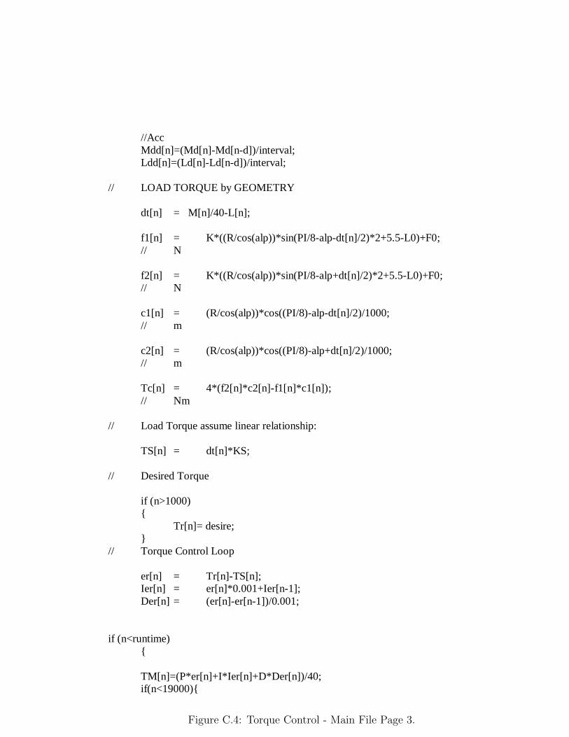
//Acc Mdd[n]=(Md[n]-Md[n-d])/interval; Ldd[n]=(Ld[n]-Ld[n-d])/interval; // LOAD TORQUE by GEOMETRY dt[n] = M[n]/40-L[n]; f1[n] = K*((R/cos(alp))*sin(PI/8-alp-dt[n]/2)*2+5.5-L0)+F0; // N f2[n] = K*((R/cos(alp))*sin(PI/8-alp+dt[n]/2)*2+5.5-L0)+F0; // N c1[n] = (R/cos(alp))*cos((PI/8)-alp-dt[n]/2)/1000; // m c2[n] = (R/cos(alp))*cos((PI/8)-alp+dt[n]/2)/1000; // m Tc[n] = 4*(f2[n]*c2[n]-f1[n]*c1[n]); // Nm // Load Torque assume linear relationship: TS[n] = dt[n]*KS; // Desired Torque if (n>1000) { Tr[n]= desire; } // Torque Control Loop er[n] = Tr[n]-TS[n]; Ier[n] = er[n]*0.001+Ier[n-1]; Der[n] = (er[n]-er[n-1])/0.001; if (n<runtime) { TM[n]=(P*er[n]+I*Ier[n]+D*Der[n])/40; if(n<19000){
Figure C.4: Torque Control - Main File Page 3.

if (TM[n]<1.3) { if (TM[n]>0) { V[n]=TM[n]*4/1.3+fr*4; Analog_Out(0,V[n]); } else { V[n]=TM[n]*4/1.3-fr*4; Analog_Out(0,V[n]); } }} else {Analog_Out(0,0);} } if (n>= runtime) flag=FALSE; } void Analog_Out (int channel, double voltage) { // check voltage double t_voltage=0.0; int dig; // make sure motor signal is between -10v to +10v if (voltage >10.0) t_voltage = 10.0; else if (voltage < -10.0) t_voltage = -10.0; else t_voltage = voltage; dig = (int)(8191 * (t_voltage+10)/20.0); //write to DAC Channel RtWritePortUshort( (PUSHORT) (DAC0), (USHORT)dig); } //Initialise encoders void RltZeroCntr(int channel) {
Figure C.5: Torque Control - Main File Page 4.

PUCHAR addresspuc, addresspuc1; addresspuc = (PUCHAR)(STG_A + channel*2); //select CNTi.C RtWritePortUchar(addresspuc, (UCHAR)0x20); //Master Control Register. MRST master reset RtWritePortUchar(addresspuc, (UCHAR)0x68); //Input Control Register. RtWritePortUchar(addresspuc, (UCHAR)0x80); //Output Control Register. RtWritePortUchar(addresspuc, (UCHAR)0xc3); //Quadrature Register 4x quadrature mode RtWritePortUchar(addresspuc, (UCHAR)0x04); //Reset encoder counters to zero. addresspuc1=(PUCHAR)(STG_A+ 0x400 + 0x0e); //TMRCMD RtWritePortUchar(addresspuc1, (UCHAR)0x3a); //chose timer 0 RtWritePortUchar(addresspuc1, (UCHAR)0x7a); //chose timer 1 RtWritePortUchar(addresspuc1, (UCHAR)0xba); //chose timer 2 printf("ENCODER %d Initialization COMPLETE\n",channel); return; } //Read encoder counter i. Return counter reading value long RltReadCntr(int channel) { PUCHAR addresspuc, addresspuc1; UCHAR cntl; UCHAR cntm; UCHAR cnth; long cntr; addresspuc = (PUCHAR)(STG_A + channel*2); //select CNTi.C //printf("\t%uc",&addresspuc); RtWritePortUchar(addresspuc,(UCHAR)0x02); //transfer counter to latch addresspuc1 = (PUCHAR)(STG_A+ channel*2 - 2); //select CNTi.D cntl = RtReadPortUchar(addresspuc1); //read counter latch low 8 bit cntm = RtReadPortUchar(addresspuc1); //read counter latch medium 8 bit cnth = RtReadPortUchar(addresspuc1); //read counter latch high 8 bit cntr=(long) (((cntl << 8) + (cntm << 16) + (cnth << 24)) / 256); return(cntr); }
Figure C.6: Torque Control - Main File Page 5.

int main() { LARGE_INTEGER x; LARGE_INTEGER Period; HANDLE hTimer; // HANDLE hToSharedMemory; RltZeroCntr(1); RltZeroCntr(3); printf("\n\nPlz Wait...\n"); Period.QuadPart=10000*p; if (!(hTimer = RtCreateTimer(NULL,0,TimerJob1,NULL,RT_PRIORITY_MAX,CLOCK_FASTEST))) // Always use fastest available clock { printf("SHUTDOWN: ERROR: Could not create the timer.\n"); ExitProcess(1); } if (!RtSetTimerRelative( hTimer, &Period, &Period)) { printf("SHUTDOWN: ERROR: Could not set and start the timer.\n"); ExitProcess(1); } printf("J = %2.4f kgm^2\n",Js); //printf ("G = %2.4f N\n",Gb2); printf("Kff = %4.2f Nm/rad\n",KS); // printf("sampling time = %3.4f s\n",interval); printf("P=%1.3f\tI=%2.3f\tD=%1.4f\n",P,I,D); printf("t(ms)\tM\tL\tdt\t\tMd(rpm)\tLdd\t\tTM(Nm)\t\tTd(Nm)\tTS(Nm)\n"); while(flag) { printf("%3.3f\t%3.4f\t%3.4f\t%3.4f\t\t",n*p*0.001,M[n],L[n],dt[n]); printf("%3.4f\t%3.4f\t\t",Md[n]*60/(2*PI),Ldd[n]); // Motor speed (rpm), Output Acc (rad/s^2) printf("%3.4f\t\t%3.4f\t%3.4f\n",V[n]*52/4,Tr[n],TS[n]);// Toutput , Tdesired Sleep(1); } RtCancelTimer(hTimer, &x); RtDeleteTimer(hTimer);
Figure C.7: Torque Control - Main File Page 6.

Appendix D
Controller Code Part III - Force
Control
D.1 Force Control
116

D.1.1 Force Control - Header File
// FORCE CONTROL FOR CONTACT START AND MOVING TO CONTACT // By: Eddie Chai // Header File // Control Architecture // Tm = [PID]*(Tl-Td) , where Tl = Ks(M-L) // Dynamics of Actuator // Tm = Tl + frictions // Tl = m*g*l*sin(L) + m*l^2*Ldd #define KS 426.0 #define PI 3.14159265359 #define Op .1 //Outer Control Gain #define Oi 0 #define Od 0 #define P 1.0 //inner Control Gain #define I 30.0 #define D 0.0 #define desire 10.0 //step //#define desire 20*sin((2*PI)*n/500) // Sinusoidal #define fr 0//0.09 // Static/holding torque (% of Tm,max) //************** ServoToGo ************************************** #define STG_A 0x240 // ServoToGo Card A base address #define STGOff 0x400 // offset for high address space #define DAC0 0x250 // Analog Out Address #define D_DIR 0x647 #define START_CONV ((PUSHORT) (STG_A+0x410)) #define PORT_ADC ((PUSHORT) (STG_A+0x410)) #define BRDTST ((PUSHORT) (STG_A+0x403)) #define pSharedMemory "SharedMemory" #define CNTRL0 ((PUSHORT) (STG_A+0x401)) typedef struct Data { int handshake; BOOL startrtss; BOOL killRT; } DATASTRUCT; DATASTRUCT *pdata;
Figure D.1: Force Control: Header File.

D.1.2 Force Control - Main File
// FORCE CONTROL FOR CONTACT START AND MOVING TO CONTACT // By: Eddie Chai // Main console #include "stdafx.h" #include <iostream.h> #include <windows.h> #include <stdio.h> #include <conio.h> #include <stdlib.h> #include <fstream.h> #include <math.h> #include <rtapi.h> #include "motorcntlrtx.h" HANDLE hshmData; HANDLE hSharedMem; // Elastic Flywheel double f1[50000]; // Force in Spring 1 (N) double f2[50000]; // Force in Spring 2 (N) double dt[50000]; // Deflection of Flywheel (rad) double c1[50000]; // Tangential Distance of Spring 1 relative to center of ff(mm) double c2[50000]; // Tangential Distance of Spring 2 relative to center of ff(mm) double Tc[50000]; // Output Torque // Dynamics of Actuator double Pot1 [50000]; double Pot [50000]; double M [50000]; // Position of Motor (rad) double L [50000]; // Position of Load (rad) double Md [50000]; // Speed of Motor (rad/s) double Mdd [50000]; // Acceleration of Motor (rad/s^2) double Ld [50000]; // Speed of Load (rad/s) double Ldd [50000]; // Acceleration of Load (rad/s^2) // Torque double TM[50000]; // Motor Torque
Figure D.2: Force Control: Main File Page 1.

double TS[50000]; // Output Torque - assume linear i.e. T = K*theta double Tr[50000]; // Desire Torque double To[50000]; // Torq computed by Outer double Tf[50000]; // force from pot // PID parameters double er[50000]; double Ier[50000]; double Der[50000]; double Oer[50000]; double OIer[50000]; double ODer[50000]; // Voltage double V[50000]; int d = 1; // delay int p = 1 ; // interval time int runtime =50000/p; int n=0; double voltage; double interval = 0.001*p*d; //interval time BOOL flag=TRUE; BOOL start=TRUE; void Analog_Out (int channel, double voltage) { // check voltage double t_voltage=0.0; int dig; // make sure motor signal is between -10v to +10v if (voltage >10.0) t_voltage = 10.0; else if (voltage < -10.0) t_voltage = -10.0; else t_voltage = voltage; dig = (int)(8191 * (t_voltage+10)/20.0);
Figure D.3: Force Control: Main File Page 2.

//write to DAC Channel RtWritePortUshort( (PUSHORT) (DAC0), (USHORT)dig); } //Initialise encoders void RltZeroCntr(int channel) { PUCHAR addresspuc, addresspuc1; addresspuc = (PUCHAR)(STG_A + channel*2); //select CNTi.C RtWritePortUchar(addresspuc, (UCHAR)0x20); //Master Control Register. MRST master reset RtWritePortUchar(addresspuc, (UCHAR)0x68); //Input Control Register. RtWritePortUchar(addresspuc, (UCHAR)0x80); //Output Control Register. RtWritePortUchar(addresspuc, (UCHAR)0xc3); //Quadrature Register 4x quadrature mode RtWritePortUchar(addresspuc, (UCHAR)0x04); //Reset encoder counters to zero. addresspuc1=(PUCHAR)(STG_A+ 0x400 + 0x0e); //TMRCMD RtWritePortUchar(addresspuc1, (UCHAR)0x3a); //chose timer 0 RtWritePortUchar(addresspuc1, (UCHAR)0x7a); //chose timer 1 RtWritePortUchar(addresspuc1, (UCHAR)0xba); //chose timer 2 printf("ENCODER %d Initialization COMPLETE\n",channel); return; } //Read encoder counter i. Return counter reading value double RltReadCntr(int channel) { PUCHAR addresspuc, addresspuc1; UCHAR cntl; UCHAR cntm; UCHAR cnth; long cntr; addresspuc = (PUCHAR)(STG_A + channel*2); //select CNTi.C //printf("%1d\n",channel); RtWritePortUchar(addresspuc,(UCHAR)0x02); //transfer counter to latch
Figure D.4: Force Control: Main File Page 3.

addresspuc1 = (PUCHAR)(STG_A+ channel*2 - 2); //select CNTi.D cntl = RtReadPortUchar(addresspuc1); //read counter latch low 8 bit cntm = RtReadPortUchar(addresspuc1); //read counter latch medium 8 bit cnth = RtReadPortUchar(addresspuc1); //read counter latch high 8 bit cntr=(long) (((cntl << 8) + (cntm << 16) + (cnth << 24)) / 256); return(cntr); } void RTFCNDCL TimerJob1(PVOID unused) { if(start) { n=0; start=FALSE; } // Initial conditions Pot[0] =0; M[0] =0; L[0] =0; Ier[0] =0; er[0] =0; Der[0] =0; n+=1; // Positions in radian M[n]=RltReadCntr(1)*2*PI/10000; L[n]=RltReadCntr(3)*2*PI/10000; Pot[n]=(convert_from_digital(Analog_In(1)))*(-47.024) -57.664; Pot1[n]=(convert_from_digital(Analog_In(0))); //Speeds in rad/s Md[n]=(M[n]-M[n-d])/interval; Ld[n]=(L[n]-L[n-d])/interval; //Acc Mdd[n]=(Md[n]-Md[n-d])/interval; Ldd[n]=(Ld[n]-Ld[n-d])/interval; // LOAD TORQUE by GEOMETRY dt[n] = M[n]/40-L[n];
Figure D.5: Force Control: Main File Page 4.

f1[n] = K*((R/cos(alp))*sin(PI/8-alp-dt[n]/2)*2+5.5-L0)+F0; // N f2[n] = K*((R/cos(alp))*sin(PI/8-alp+dt[n]/2)*2+5.5-L0)+F0; // N c1[n] = (R/cos(alp))*cos((PI/8)-alp-dt[n]/2)/1000; // m c2[n] = (R/cos(alp))*cos((PI/8)-alp+dt[n]/2)/1000; // m Tc[n] = 4*(f2[n]*c2[n]-f1[n]*c1[n]); // Nm Tf[n] = Pot[n]; // Load Torque assume linear relationship: TS[n] = dt[n]*KS; // Desired Torque if (n>0) { Tr[n]= desire; } // Outer Force Control Loop Oer[n] = Tr[n]-Tf[n]; OIer[n]= er[n]*0.001+Ier[n-1]; ODer[n] = (er[n]-er[n-1])/0.001; To[n] = (Op*Oer[n]+Oi*OIer[n]+Od*ODer[n]); // inner Torque Control Loop er[n] = To[n]-TS[n]; Ier[n] = er[n]*0.001+Ier[n-1]; Der[n] = (er[n]-er[n-1])/0.001; if (n<runtime) { TM[n]=(Op*Oer[n]+Oi*OIer[n]+Od*ODer[n])/40; //rigid //TM[n]=(P*er[n]+I*Ier[n]+D*Der[n])/40; //elas if(n<19000){
Figure D.6: Force Control: Main File Page 5.

if (TM[n]<.65) { if (TM[n]>0) { V[n]=TM[n]*4/1.3+fr*4; // Analog_Out(0,V[n]); } else { V[n]=TM[n]*4/1.3-fr*4; // Analog_Out(0,V[n]); } }} else {Analog_Out(0,0);} } if (n>= runtime) flag=FALSE; } void CalADC(void) { UCHAR ctrl0; RtWritePortUchar((PUCHAR)(D_DIR),(UCHAR)0x8b); //Initialize register D_DIR to enable writing on CNTRL0 RtPrintf("Configure D_DIR register successful...\n"); Sleep(10); //Wait for the command to settel ctrl0=RtReadPortUchar((PUCHAR)CNTRL0) & 0x07; //Get CNTRL0 value and save the IRQ RtWritePortUchar((PUCHAR)CNTRL0,ctrl0); //cal is low RtWritePortUchar((PUCHAR)CNTRL0,(UCHAR)(ctrl0|0x08)); //cal is high Sleep(10); } //This implementation is according to STG version2.0 //Refer to manual pp. 31 for more detail int Analog_In(int channel) { //for port I/O code
Figure D.7: Force Control: Main File Page 6.

int count=0; USHORT sX, temp; UCHAR ctrl0; int sign; int ret; //Step 1 & 2: Set multiplexer (CNTRL0) and wait for 4 us ctrl0 =RtReadPortUchar((PUCHAR)(CNTRL0)) & 0x07; //Save irq (last 3 bits) ctrl0 |= (channel<<4) | 0x88; //Select channel to perform conversion (channel = 0,1,2) RtWritePortUchar((PUCHAR)(CNTRL0),ctrl0); //Send command to CNTRL0 //STEP 3: Start conversion by send dummy value to START_CONV RtWritePortUshort(START_CONV, 0x00); //write to register to initiate conversion //STEP 4: Wait until conversion finish while((RtReadPortUshort(BRDTST) & 0x08) && count<10000); { count++; //wait for /EOC } //STEP 5: Reading sX = RtReadPortUshort(PORT_ADC); sX = sX & 0x1fff; sign = sX & 4096; if (sign) { temp = (~sX & 0x1fff) +1; ret = -temp; } else ret = sX; return (ret); } /* working in degreees 0 == -10V == -120 degrees 4096*2(8192) == 10V == 120 deg */ double convert_from_digital(int dig)
Figure D.8: Force Control: Main File Page 7.

{ return (10*(dig+4096)/8192.0 - 5.0); } int main() { LARGE_INTEGER x; LARGE_INTEGER Period; HANDLE hTimer; // HANDLE hToSharedMemory; CalADC(); RltZeroCntr(1); RltZeroCntr(3); /***end of Pot initialisation***/ printf("\n\nPlz Wait...\n"); Period.QuadPart=10000*p; hshmData = RtCreateSharedMemory(PAGE_READWRITE, 0, sizeof(pdata), "SharedMemory", (LPVOID*) &pdata); if (!(hTimer = RtCreateTimer(NULL,0,TimerJob1,NULL,RT_PRIORITY_MAX,CLOCK_FASTEST))) // Always use fastest available clock { printf("SHUTDOWN: ERROR: Could not create the timer.\n"); ExitProcess(1); } if (!RtSetTimerRelative( hTimer, &Period, &Period)) { printf("SHUTDOWN: ERROR: Could not set and start the timer.\n"); ExitProcess(1); } //RtWritePortUchar((PUCHAR)(0x647),(UCHAR)0x8b); //so that CNTRL0 is usable...refer to the manual!!! ResumeThread(hTimer); // printf("J = %2.4f kgm^2\n",Js); //printf ("G = %2.4f N\n",Gb2);
Figure D.9: Force Control: Main File Page 8.

// printf("Kff = %4.2f Nm/rad\n",KS); // printf("sampling time = %3.4f s\n",interval); //printf("P=%1.3f\tI=%2.3f\tD=%1.4f\n",P,I,D); printf("t(ms)\tM\tL\tPOt\t\tdt\t\tMd(rpm)\tLdd\t\tTM(Nm)\t\t\tTd(Nm)\tTS(Nm)\n"); while(flag) { printf("%3.3f\t%3.4f\t%3.4f\t%5.5f\t%3.4f\t\t\n",n*p*0.001,M[n],L[n],Pot[n],dt[n]); printf("%3.4f\t%3.4f\t\t",Md[n]*60/(2*PI),Ldd[n]); // Motor speed (rpm), Output Acc (rad/s^2) printf("%3.4f\t\t%3.4f\t%3.4f\n",V[n]*52/4,Tr[n],TS[n]);// Toutput , Tdesired // printf("%3.3f\t\t%5.3f\t%5.4f\n",n*p*0.001,Pot[n],Pot1[n]); Sleep(10); } RtCancelTimer(hTimer, &x); RtDeleteTimer(hTimer); return 0; }
Figure D.10: Force Control: Main File Page 9.

Appendix E
Suppliers
This section contains a list of all the suppliers that were used in development of the
actuator.
Accord Network Services Pte. Ltd.
23, Kelantan Lane, 05-01A
Singapore 208642
Tel.: 9766 2038
Fax: 6294 9283
E-mail: [email protected]
servomotors, gearbox
Yong Seng Screws Pte. Ltd.
Blk 802 01-57
French Road,
Singapore 200802.
Tel.: 6294 1866
Fax: 6294 1178
website: www.ysscrews.com
connectors, screws
127

Heidenhain Pacific Pte. Ltd.
50, Lorong 21, Geylang,
Heidenhain Building,
Singapore 388465.
Tel.: 6749 3238
Fax: 6749 3922
encoders, encoder bearing unit
Servo Dynamics Pte. Ltd.
10, Kaki Bukit Road,
10-30 Kaki Bukit Industrial Park,
Singapore 416715.
Tel.: 6844 0288
Fax: 6844 0070
E-mail: [email protected]
website: www.servo.com.sg
servomotors, gearbox, coupling
PBA (s) Pte. Ltd.
157, Sin Ming Road,
Amtech Building(Annex Blk), 02-01,
Singapore 575624.
Tel.: 6552 7992
Fax: 6552 6992
E-mail: [email protected]
ceramic bush, ball bearings
Bosch Rexroth Pte. Ltd.
19 Kian Teck Way,
Singapore 628740.
Tel.: 6265 6033
Fax: 6265 0813
E-mail: [email protected]
Aluminum profile tube for stand

Elite Springs Industries
50 Bukit Batok st. 23
06-23/24 Midview Building
Singapore 659578.
Tel.: 6556 2252
Fax: 6566 2115
springs
Associated Spring Asia Pte. Ltd
28 Tuas Ave 2
Singapore 639459.
Tel.: 6863 5636
Fax: 6863 6325
E-mail: [email protected]
springs