Reforestation in the Cerro Candelaria Reserve: Studying the success of reforestation efforts in abandoned pastures in the

Ecuadorian Cloud Forest

Chang, Christopher A.

Supervising Academic Director: Robayo, Javier

Academic Director: Silva, Xavier Project Advisor: Bermúdez, Diana

University of Denver

Environmental Science South America, Ecuador, Tungurahua, El Placer

Submitted in partial fulfillment of the requirements for Ecuador Comparative Ecology and Conservation, SIT Study Abroad, Fall 2013

  2  

Reforestation in the Cerro Candelaria Reserve: Studying the success of reforestation efforts in abandoned pastures in the

Ecuadorian Cloud Forest

Chang, Christopher A.

ABSTRACT

This study measured the success of reforestation through data collected in November of 2013 combined with data from past studies. Deforestation is an ecological disaster that is an increasing problem across the globe. In Ecuador, the country with the highest deforestation rates in South America, the problem is particularly present. With increasing deforestation, reforestation projects are crucial to the protection of key ecosystems. This study measures the progress and effectiveness of a reforestation project managed by the Fundacion Eco-Minga in the Cerro Candelaria Reserve, which is part of the Corredor Ecologico Llangantes Sangay. Analysis of this data showed general progress of the reforestation project as well as the effectiveness of reforestation compared to primary forest and recently abandoned pasturelands.

RESUMEN

Este estudio investiga el éxito de la reforestación en la Reserva Cerro de Candelaria por datos colectados en Noviembre de 2013 combinado con datos de investigaciones pasados. Deforestación es un desastre ecológico, y es un problema que está creciendo por todo el mundo. En Ecuador, el país con la tasa más grande de deforestación en Suramérica, es muy importante estudiar este problema. Con el crecimiento de la tasa de deforestación, la reforestación tiene mucha importancia para la protección de ecosistemas muy importantes. Este estudio ha medido el progreso y eficacia de un proyecto de reforestacion manejado por la Fundacion Eco-Minga en la Reserva Cerro de Candelaria que es un parte importante del Corredor Ecologico Llangantes Sangay. Análisis de estos datos muestra progreso en el proyecto de reforestación y también la eficacia de reforestación en comparación a bosque primario y pastos que fueron abandonados recientemente.

Codes: 614, 613, 608

Keywords: reforestation, cloud forest, tree diversity

  3  

INTRODUCTION

Cloud Forest ecosystems hold much importance across the world, even though they account for only 2.5% of total tropical forests (Cayuela et. Al, 2006). They are unique ecosystems that have an incredible amount of biodiversity and provide many environmental services to the surrounding area. In Ecuador, cloud forests exist on both sides of the Andean Cordillera. This forest, found between 1,500 and 3,000 meters above sea level (Cayuela et. Al, 2006), is characterized by the high levels of humidity and the clouds that inundate the region every afternoon and evening. These forests are formed from the “rain shadow” effect created by the Andean Cordillera. As clouds approach the Andes, they must gain altitude in order to pass over the mountains. Higher altitudes correspond with lower temperatures, which in turn correspond with lower dew points. As the clouds rise, the ambient air and dew point temperatures around them drop. This leads to precipitation, as the clouds need to lessen their moisture content to rise over the mountains. This high moisture content means that soils in cloud forests are generally wet; leading to slow decomposition and generally peaty and acidic soils (Bruijnzeel and Hamilton, 2006). These ecosystems are also characterized by distinct type of vegetation. Leaves are smaller and harder, and there are a immense amounts of epiphytes found on trees and other woody plants. Bromeliads, orchids, ferns, lichens, and mosses are all found in abundance throughout these cloud forest ecosystems (Bruijnzeel and Hamilton, 2000). When the clouds move through these forests, water condenses on the epiphytes and adds to the moisture in these ecosystems.

Cloud forests and the flora and fauna that inhabit them are extremely important to humans. The unique environment provided by the cloud forest ecosystem means that these areas have high levels of biodiversity. Many rare species call the Ecuadorian Cloud Forest home, including Spectacled Bears, Mountain Tapirs, pumas, the Andean Cock of the Rock, Giant Ant pitta, and many more (Jost). These species are heavily reliant on the cloud forest ecosystem as a habitat, and the destruction of these ecosystems could mean the extinction of many of these species. There are also very high rates of endemism in the cloud forest ecosystems; a study conducted by Steven Churchill calculated the endemism of the tropical Andes to be about 31% of all floral species (Churchill, 2009). This is an astronomically high rate of endemism, and many of those endemic species are found in cloud forests such as those in Ecuador. In addition, these forests are severely lacking in scientific research and exploration. Over the last several years, botanist Lou Joust and his team have found over 28 species of Teagueia orchids that are both new to science and endemic to one mountain in south western Ecuador (Jost). These discoveries demonstrate the dearth of research on the cloud forest ecosystem; if 28 new species can be found on just one mountain, the amount of unknown species across all cloud forest ecosystems must be immense. This biodiversity is important to the planet in that evolution is built upon genetic diversity and it is likely that this biodiversity will also have direct and tangible benefits to humans. Many crops that are used for human consumption such as strawberries, blueberries, raspberries, and gooseberries have relatives that can be found growing wild in the cloud forest. By breeding hybrids between these wild varieties and the common varieties, these crops can be strengthened and more effectively cultivated (Bruijnzeel and Hamilton, 2000). Also, many medicines are derived from naturally growing plants, particularly those growing in tropical regions. For example, many amoebicides, antimalarials, and anesthetics are refined chemicals found in the flora of tropical forests. These medicines, and others derived from plants native to the tropics, have obvious and far reaching therapeutic benefits. They also have huge

  4  

economic worth; collectively being worth over 35 billion British pounds annually (Caldecott, 1987). Due to the hostile environment of the tropics, plants have evolved unique chemicals to defend themselves against predators. Often these chemicals have medicinal uses for humans, meaning that more time in the field, rather than in a lab, is most likely the best way to yield new medicines (Caldecott, 1987). This highlights the importance of conserving these tropical environments, as it is very possible that some of the unknown species endemic to these cloud forests have medicinal properties that could benefit all of mankind.

Unfortunately, cloud forests across the world are in serious danger. They are being deforested at an unprecedented rate, and as they are deforested, all the biodiversity and endemism associated with them is being lost. In the Andes, cloud forests are cleared for many reasons, including logging, fuelwood, agriculture, and grazing (Jokisch and Lair, 2002). One study of a 187 square kilometer region of typical Ecuadorian cloud forest indicated that over 400 hectares of cloud forest had been converted to pasture in only 11.5 years (Jokisch and Lair, 2002). These astronomically high rates of deforestation have many roots in governmental policies encouraging destructive land use in favor of high productivity (Pinchon, 1997). In 1973, the Ecuadorian government passed a law requiring that 80% of all arable land be productive. The law also forced land owners to pay a tax of $10 per hectare for any unproductive land. This, as well as other agrarian reforms, has been instrumental in promoting the deforestation of fragile cloud forest ecosystems at an unprecedented rate.

Typically, rural small scale agriculture in Ecuador consists of traditional slash and burn practices. Slash and burn agriculture refers to the practice of clear-cutting a patch of land, burning the biomass accumulated on the ground, and then planting crops. Once all of the nutrients in the soil are used and the land becomes unproductive, the field is abandoned and left to regenerate. Unfortunately, societal pressures have changed the types of crops being grown on these plots. Typical subsistence crops such as corn, beans, and potatoes have been replaced with cash crops such as naranjilla and pasturelands for grazing cattle. These pastures and cash crop plots are more nutrient intensive, and because of this natural regeneration after the plots are abandoned is a very slow process (Knoke et. Al, 2009). Historically, small indigenous populations could sustain this style of slash and burn agriculture, however, rising populations and more intensive crops and cultivation methods have led to vastly higher rates of deforestation than natural regeneration. According to one study of rural agriculture in Ecuador, traditional land use strategies over the course of one generation of farmers (40 years) would lead to over 18.3 hectares of deforestation (Knoke et. Al, 2009). These land-intensive practices and growing populations of farmers are causing extremely high deforestation rates which are threatening the existence of cloud forests across South America.

The Fundacion Eco-Minga was created in 2006 with the goal of preserving Ecuador’s delicate ecosystems and restoring disturbed land to its natural state, particularly in the Tungurahua province of eastern Ecuador and the Upper Pastaza watershed. Currently, the foundation has bought land to create 6 reserves: Cerro Candelaria, Rio Anzu, Rio Zunac, Brand Stand, Rio Valencia, and Naturetrek (Jost, Robayo, and Reyes, 2010). These reserves were created as the beginning of a biological corridor between the Parque Nacional Llanganates in the North, and Parque Nacional Sangay in the south called the Corredor Ecologico Llanganates Sangay. This biological corridor will provide an important throughway for the flora and fauna of each of these parks, extending the range of all of the important species that depend on these

  5  

parks for habitat (Tewksbury, Douglas, Haddad, Sargent, Orrock, Weldon, Danielson, and Brinkerhoff, 2002). The efforts of Eco-Minga in creating this biological corridor are crucial to reducing the effects of fragmentation caused by the unprotected land between the two National Parks, as well as restoring the land to its original state.

Project Background

The Cerro Candelaria Reserve was purchased by Eco-Minga in 2007. The reserve is located just south of El Placer, a town of approximately 400 inhabitants located 6 km east from the town of Baños. The reserve is comprised of around 2600 hectares and current expansion efforts are in progress as well. The Cerro Candelaria Reserve contains 16 abandoned pastures that are in different stages of reforestation. These abandoned pastures were all reforested between 2008 and 2010 using different reforestation techniques. When Eco-Minga first acquired the land, all of the pastures were completely overrun with African grasses, with very few native trees left standing. Because of these aggressive grasses, it was necessary to treat the pastures with glyphosate (in the form of Round-up or Ranger) before reforestation efforts were started. Glyphosate is a wide spectrum herbicide which blocks an essential enzyme which aids in the synthesis of amino acids in the plant. It is relatively safe and is not known to cause harm to animals or to reduce fertility of the land, as it only targets actively growing plants. Glyphosate was used to lessen the strength of the competition of the well-established pastoral grasses and give the reforested saplings a better chance of success. Often, reforestation efforts involve the use of a greenhouse in order to grow seedlings to a more competitive size before they are planted. Unfortunately, due to the remoteness and topography of this site, construction of a greenhouse was not possible in this location. Instead, seedlings were gathered from surrounding primary forest and relocated to the sites of reforestation. The project deliberately chose trees that grow quickly and are beneficial to the local fauna: large seeded lauraceae account for many of the species due to their rapid growth rates and the fact that they provide food for many different types of rare birds. Biodiversity was also a consideration of the project and an effort was made to use over thirty different types of trees including at least one endemic species (Jost, 2008).

After the saplings were collected from the surrounding forest they were placed in plastic bags full of local soil and put in at the forest edge for several months to recover from the transplant trauma. After a few months of recovery, the saplings were transplanted to the pastures. The saplings were periodically protected from the aggressive African grasses by hand-weeding and spot treatments of glyphosate (Jost, 2008). Also, the park guards continue to actively encourage growth of these saplings by cleaning them approximately once a year which involves cutting back other species in competition with the planted trees.

METHODS

In order to investigate the overall success of reforestation attempts in the Cerro Candelaria reserve, standard forestry methods were used to determine diversity and tree growth in 16 plots. This project measured the diameter at breast height (DBH), the actual height of the tree, the location of each tree on a Cartesian x,y plane, and recorded the species of each tree measured. 14 of the 16 plots quadrants were previously established for prior reforestation research. These quadrants were generally established along the main trail and were 10 by 10 meters. Once the plots were re-established, which required a trail to be made with a machete between markers, measurements of each tree in the quadrants were taken. The DBH was

  6  

measured at the standard 1.3 meters above the ground using a specifically designed measuring tape that converts circumference into diameter. The height was measured using a Bosch DLR130 distance measurer: the researcher would adjust the laser to rest on the highest leaf of the tree, measure the distance, and then turn the device over to record the distance from the ground to the device. These two measurements added together give the total height of the tree. DBH was measured in centimeters and the height was measured in meters. The location of each tree was recorded in x, y coordinates with “0,0” at the bottom left corner of the transect. The species of each tree was determined by comparing the trees to pictures. The pictures were taken on an initial walk through of the site and each type of tree was identified and catalogued by park guard Jesus Recalde. Most trees were identified in the field though several were unknown. After each tree was recorded, it was marked with tape in order to eliminate the possibility of double counting, as well as to catalogue which trees had been counted for future reforestation research of the area. GPS points of each quadrant were also taken at the southwestern most point of the quadrant in order to facilitate future research.

Several different indices and formulas were used to analyze the collected data. First, the standard diversity indices of Margalef, Simpson, and Shannon- Wiener were calculated.

The Margalef index represents the species richness in a given population:

𝐷! = (𝑆 − 1)/log  (𝑁)

Where S represents the number of species in the population, and N represents the number of individuals.

The Simpson index represents the diversity of a given population in terms of the likelihood that a sampling of two random individuals produces the same species:

𝐷! = 1− 𝑃!!

Where 𝑃!represents the relative frequency of individuals of each different species in a population.

The Simpson Index has a range of 0 to 1 where zero represents a sample with no diversity, and one represents a sample of infinite diversity. The function, however, is logarithmic so the actual range is 0<X<1

The Shannon-Wiener Diversity Index represents diversity in terms of abundance of different species as well as evenness of the sample:

𝐻′ = − 𝑃! ln𝑃!

Where 𝑃!  is the same as in the Simpson Index: representing the relative frequency of individuals of each different species in a population

These three indices all measure diversity in some capacity, however, they also all take slightly different diversity factors into consideration in their calculations. Because of these differences,

  7  

when all of the indices are looked at together they can give a more complete picture of diversity than any one index could individually.

In addition to these three standard measures of diversity a new method of calculating diversity, which was recently proposed by Lou Jost, was also used. He posits that the most effective way to compare diversity is by comparing effective number of species in different samples (Jost). In order to calculate effective number of species for each plot the inverse of the Simpson Index was taken:

𝐷! =1

(1− 𝑃!!)

Where 𝑃!  represents the relative frequency of individuals of each different species in a population.

In order to compare the similarity of the quadrants to each other, the Jaccard Index was also used:

𝐽 =𝐴

𝐴 + 𝐵 + 𝐶

Where A represents the total number of species present in both communities, B represents the number of species represented in the first community but absent from the second, and C represents the number of species represented in the second community but absent from the first.

This index is useful for comparing the differences between each of the different plots in terms of composition. Looking at all of these different indices will allow for a meaningful comparison of diversity and composition between the different plots and strategies of reforestation in Cerro Candelaria.

Materials

1. Measuring tape 2. DBH tape 3. Bosch DLR130 Distance Measurer 4. Marking tape 5. Camera 6. GPS

SITE DESCRIPTION

This reforestation effort has taken place in the northernmost part of the Cerro Candelaria Reserve. There are 16 plots, labeled A-P, that have been established and were reforested between mid-2008 and late 2009. The altitudes of the plots range from 1840 meters above sea level to 2120 meters above sea level (approximately 6,000 - 7,000 feet). The distance between primary forest and Plot P is 1260 meters along the primary trail. All but three of the established quadrants are located right along the trail with the quadrant for Plot H located just off the trail. Plots A and

  8  

B are located above the primary trail and require more hiking up a secondary trail to reach the sites. The plots located on the west side of the trail are on the downward slope of the mountain, and those located on the east side are located above the trail.

Figure 1. Map of Reforestation Plots This map shows the reforested pastures (Plot A is the furthest south, Plot P is furthest north and closest to the Eco-Minga Cabin). The yellow dots represent the GPS points of each quadrant.

Plot List

Plot A: This plot was established in May of 2008 and is the furthest plot from the main trail. It has been established as a site of natural regeneration. Before Eco-Minga established this reforestation effort this area was pasture. GPS Coordinates of the site are 799050/ 9841723. Elevation is 2058 meters. Plot B: This plot was established in July of 2008. Before being planted this plot was treated with glyphosate (in the form of Round-up or Ranger). This site is also located off of the main trail, and was previously pasture. GPS coordinates of the site are 798687/9840730. Elevation is 1897 meters.

  9  

Plot C: This plot was established in August of 2008. This site was treated with glyphosate and was previously a pasture. GPS coordinates of the site are 798670/9840789. Elevation is 1890 meters. Plot D: This plot was established in September of 2008. This site was treated with glyphosate and was previously pasture. GPS coordinates of the site are 798697/9840962. Elevation is 1883 meters. Plot E: This plot was established in October of 2008. This site was treated with glyphosate and was previously pasture. GPS coordinates of the site are 798690/9841029. Elevation is 1888 meters. Plot F: This plot was established in December of 2008. This site was treated with glyphosate and was previously pasture. GPS coordinates of the site are 798670/9851090. Elevation is 1879 meters. Plot G: This plot was established in January of 2009. This site was treated with glyphosate and was previously pasture. GPS coordinates of the site are 798660/ 9841277. Elevation is 1890 meters. Plot H: This plot was established in September of 2009. This site was treated with glyphosate and was previously pasture. GPS coordinates of the site are 798688/9841452. Elevation is 1904 meters. Plot I: This plot was established in October of 2009. This site was not treated with glyphosate like the others, but similarly it was previously pasture. GPS coordinates of the site are 798735/9841481. Elevation is 1904 meters. Plot J: This plot was established in October of 2009. This site was not treated with glyphosate either. Also, this site was previously a naranjilla farm, not a pasture. GPS coordinates of the site are 798802/9841501.Elevation is 1912 meters. Plot K: This plot was established in October of 2009. This site was treated with glyphosate and was previously pasture. GPS coordinates of the site are 798862/9841541. Elevation is 1915 meters. Plot L: This plot was established in November of 2009. This site was treated with glyphosate and was previously pasture. GPS coordinates of the site are 798939/9841580. Elevation is 1904 meters. Plot M: This plot was previously a pasture but no reforestation efforts have taken place here. GPS coordinates of the site are 798975/9841668. Elevation is 1916 meters. Plot O: This plot was established as another natural regeneration experiment. It is located right on the trail and directly adjacent to the Eco-Minga Cabin. GPS coordinates of the site are 799050/9841723. Elevation is 1899 meters. Plot P: This plot was established in November 2009. This site was treated with glyphosate and was previously a naranjilla farm. GPS coordinates of the site are 799021/9841698. Elevation is 1897 meters.

Note: GPS coordinates represent the southwestern most corner of each sampled quadrant. In relation to the main trail, it is the corner furthest from the cabin and highest on the mountain.

  10  

RESULTS Tree Distribution Figures 2-16 show the distribution of trees within each measured quadrant. Plots C and D had the most uniform distribution, while Plots F and J had trees that were more clumped together. Plots A and L, and the Primary Forest had very random distributions.    

Figure  2                 Figure  3  

 

   

Figure  4                 Figure  5                

0  1  2  3  4  5  6  7  8  9  10  

0   1   2   3   4   5   6   7   8   9   10  

Plot  A  Distribu-on  

0  1  2  3  4  5  6  7  8  9  10  

0   1   2   3   4   5   6   7   8   9   10  

Plot  B  Distribu-on  

0  1  2  3  4  5  6  7  8  9  10  

0   1   2   3   4   5   6   7   8   9   10  

Plot  D  Distribu-on  

0  1  2  3  4  5  6  7  8  9  10  

0   1   2   3   4   5   6   7   8   9   10  

Plot  C  Distribu-on  

  11  

0  1  2  3  4  5  6  7  8  9  

10  

0   1   2   3   4   5   6   7   8   9   10  

Plot  F  Distribu-on    

 

 

 

 

 

 

Figure  6                 Figure  7  

 

 

 

 

 

 

 

 

Figure  8                 Figure  9  

 

 

 

 

 

 

 

Figure  10               Figure  11  

0  1  2  3  4  5  6  7  8  9  10  

0   1   2   3   4   5   6   7   8   9   10  

Plot  E  Distribu-on  

0  1  2  3  4  5  6  7  8  9  10  

0   1   2   3   4   5   6   7   8   9   10  

Plot  H  Distribu-on  

0  1  2  3  4  5  6  7  8  9  10  

0   1   2   3   4   5   6   7   8   9   10  

Plot  G  Distribu-on  

0  1  2  3  4  5  6  7  8  9  10  

0   1   2   3   4   5   6   7   8   9   10  

Plot  J  Distribu-on  

0  1  2  3  4  5  6  7  8  9  10  

0   1   2   3   4   5   6   7   8   9   10  

Plot  I  Distribu-on  

  12  

 

 

 

 

 

 

 

 

Figure  12               Figure  13  

 

 

 

 

 

 

 

 

Figure  14                 Figure  15  

 

 

Figure  16  

 

 

Figures  2-­‐16:  Tree  distribution  within  each  of  the  10X10  quadrants  

0  1  2  3  4  5  6  7  8  9  

10  

0   1   2   3   4   5   6   7   8   9   10  

Plot  L  Distribu-on  

0  1  2  3  4  5  6  7  8  9  

10  

0   1   2   3   4   5   6   7   8   9   10  

Plot  P  Distribu-on  

0  1  2  3  4  5  6  7  8  9  10  

0   1   2   3   4   5   6   7   8   9   10  

Primary  Forest  Distribu-on  

0  1  2  3  4  5  6  7  8  9  10  

0   1   2   3   4   5   6   7   8   9   10  

Plot  K  Distribu-on  

0  1  2  3  4  5  6  7  8  9  10  

0   1   2   3   4   5   6   7   8   9   10  

Pasture  (Plot  M)  Distribu-on  

  13  

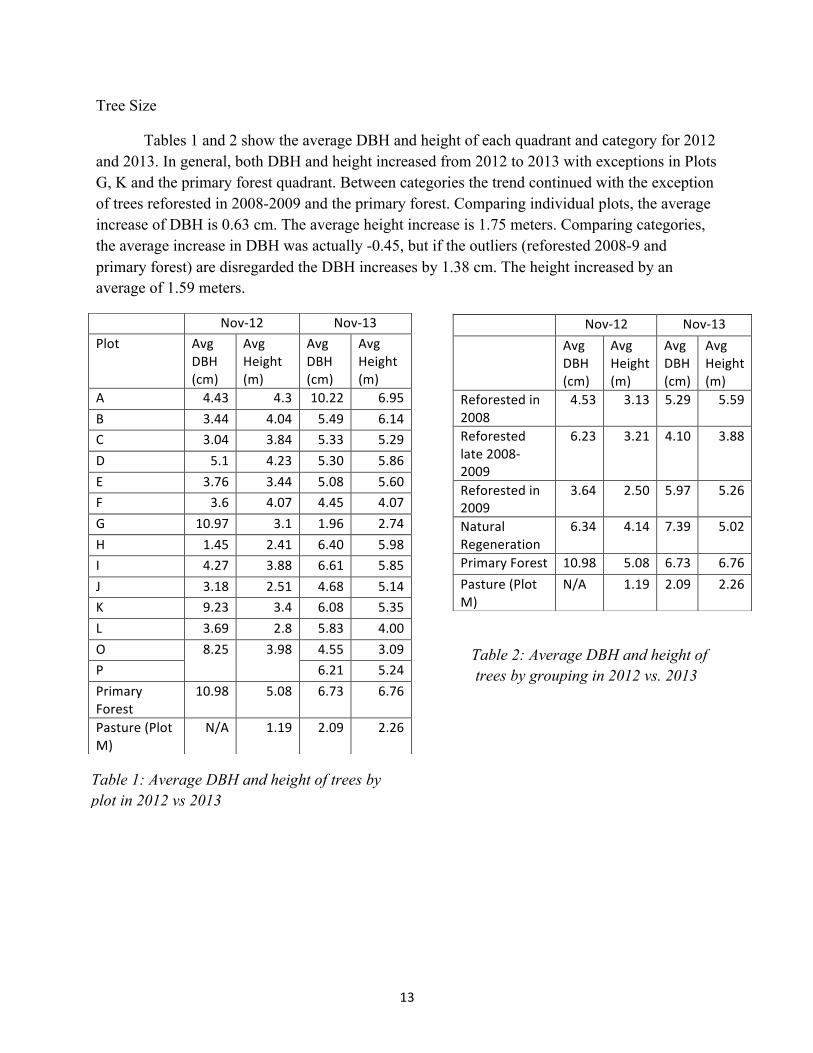
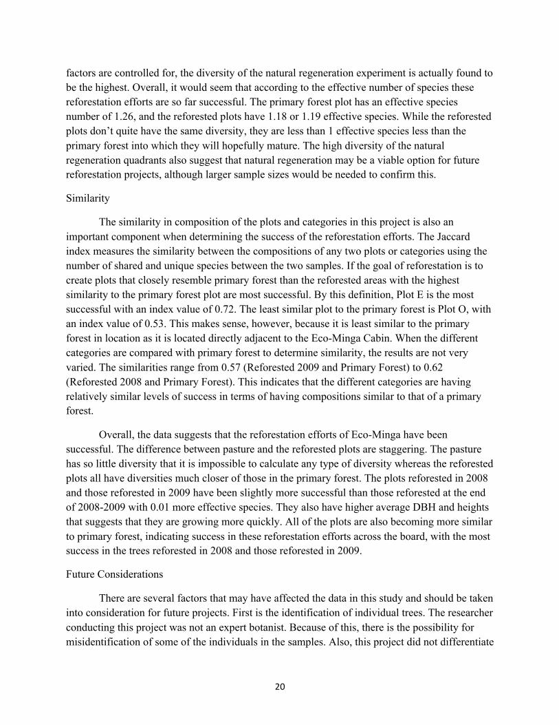
Tree Size

Tables 1 and 2 show the average DBH and height of each quadrant and category for 2012 and 2013. In general, both DBH and height increased from 2012 to 2013 with exceptions in Plots G, K and the primary forest quadrant. Between categories the trend continued with the exception of trees reforested in 2008-2009 and the primary forest. Comparing individual plots, the average increase of DBH is 0.63 cm. The average height increase is 1.75 meters. Comparing categories, the average increase in DBH was actually -0.45, but if the outliers (reforested 2008-9 and primary forest) are disregarded the DBH increases by 1.38 cm. The height increased by an average of 1.59 meters.

 

Table 2: Average DBH and height of trees by grouping in 2012 vs. 2013

 

 

  Nov-­‐12   Nov-­‐13  Plot   Avg  

DBH  (cm)  

Avg  Height  (m)  

Avg  DBH  (cm)  

Avg  Height  (m)  

A   4.43   4.3   10.22   6.95  B   3.44   4.04   5.49   6.14  C   3.04   3.84   5.33   5.29  D   5.1   4.23   5.30   5.86  E   3.76   3.44   5.08   5.60  F   3.6   4.07   4.45   4.07  G   10.97   3.1   1.96   2.74  H   1.45   2.41   6.40   5.98  I   4.27   3.88   6.61   5.85  J   3.18   2.51   4.68   5.14  K   9.23   3.4   6.08   5.35  L   3.69   2.8   5.83   4.00  O   8.25   3.98   4.55   3.09  P   6.21   5.24  Primary  Forest  

10.98   5.08   6.73   6.76  

Pasture  (Plot  M)  

N/A   1.19   2.09   2.26  

  Nov-­‐12   Nov-­‐13     Avg  

DBH  (cm)  

Avg  Height  (m)  

Avg  DBH  (cm)  

Avg  Height  (m)  

Reforested  in  2008  

4.53   3.13   5.29   5.59  

Reforested  late  2008-­‐2009  

6.23   3.21   4.10   3.88  

Reforested  in  2009  

3.64   2.50   5.97   5.26  

Natural  Regeneration  

6.34   4.14   7.39   5.02  

Primary  Forest   10.98   5.08   6.73   6.76  Pasture  (Plot  M)  

N/A   1.19   2.09   2.26  

Table 1: Average DBH and height of trees by plot in 2012 vs 2013

 

  14  

Diversity

The diversity of each quadrant and category are very varied between data collected in 2012 and 2013 (Tables 3 and 4). This study found that the diversity of each quadrant also depended heavily on which index was used. In general for 2013, Plots B and K and the primary forest were the most diverse across all indices (Plot B Da=8.89, Ds=0.89, H=1.34, Dl=1.13; Plot K Da=8.17, Ds=0.89, H=2.37, Dl=1.13; Primary forest Da=8.72, Ds=0.79, H=1.26, Dl=1.26). The pasture was by far the least diverse with all indices less than or equal to 0. When looking at diversity by category, the 2009 reforestation efforts were the most diverse (Da=110.3, Ds=0.84, H=2.28, Dl=1.19). Again, the least diverse category was the pasture.

Table 3: Diversity by plot in 2012 vs. 2013 This table shows number of species (S) number of individuals (N), Margalef Index (Da), Simpson Index (Ds), Shannon Wiener Index (H), and effective species according to Lou Jost (Dl) for each individual quadrant

 

 

 

 

Diversity  By  Plot  

Nov-­‐12   Nov-­‐13    

Category   S   N   Da   Ds   H   Dl   S   N   Da   Ds   H   Dl    Plot  A   17 31 10.73 0.93 2.75 1.08   8 23 5.14 0.77 1.72 1.30 Plot  A  Plot  B   10 28 6.22 0.81 1.93 1.24   14 29 8.89 0.89 1.34 1.13 Plot  B  Plot  C   18 93 8.64 0.77 2.10 1.30   13 72 6.46 0.80 1.56 1.25 Plot  C  Plot  D   10 29 6.15 0.80 1.93 1.25   5 20 3.07 0.75 1.47 1.33 Plot  D  Plot  E   14 54 7.50 0.76 1.92 1.32   10 41 5.58 0.81 1.72 1.24 Plot  E  Plot  F   11 29 6.84 0.86 2.08 1.17   9 31 5.36 0.83 1.81 1.21 Plot  F  Plot  G   8 45 4.23 0.32 0.81 3.13   4 5 4.29 0.72 1.33 1.39 Plot  G  Plot  H   15 43 8.57 0.81 2.13 1.23   8 34 4.57 0.56 1.28 1.80 Plot  H  Plot  I   11 34 6.53 0.83 2.04 1.21   8 30 4.74 0.83 1.89 1.20 Plot  I  Plot  J   14 48 7.73 0.57 1.53 1.75   13 45 7.26 0.80 2.01 1.26 Plot  J  Plot  K   15 48 8.33 0.76 2.01 1.32   14 39 8.17 0.89 2.37 1.13 Plot  K  Plot  L   12 48 6.54 0.62 1.58 1.62   9 14 6.98 0.85 2.04 1.18 Plot  L  Plot  O   8 24 5.07 0.77 1.70 1.29   6 6 6.43 0.83 1.79 1.20 Plot  O  Plot  P   8 8 7.75 0.88 2.08 1.14   7 29 4.10 0.79 1.69 1.27 Plot  P  Primary  Forest  

15 19 10.95 0.93 2.65 1.08   14 31 8.72 0.79 1.26 1.26 Primary  Forest  

Pasture  (Plot  M)  

2 3 2.10 0.44 0.64 2.25   1 2 0.00 0.00 -0.69 N/A   Pasture  (Plot  M)  

  15  

Table 4: Diversity by category 2012 vs. 2013 This table shows number of species (S) number of individuals (N), Margalef Index (Da), Simpson Index (Ds), Shannon Wiener Index (H), and effective species according to Lou Jost (Dl) for each category studied

Similarity

The values for the Jaccard index calculations for the individual plots (Table 5) range from 0.50-0.78. The higher numbers represent greater similarity between the given plots or categories. The most similar plots are Plots P and D (0.78), primary forest and Plot E (0.72), and Plots P and F (0.71). Jaccard index values for similarity between categories (Table 6) range from 0.50-0.70. The most similar categories are plots reforested in 2008 and plots reforested in 2009 (0.70), and the plots reforested in 2008 and those reforested at the end of 2008-2009 (0.64). The pasture quadrant was most dissimilar to the others, and when compared to all of the other plots had a value of either 0.50 or 0.51.

Table  5:  Similarity  of  categories  calculated  using  the  Jaccard  Index,  A  comparison  of  similarities  between  all  of  the  categories  of  this  project  

Diversity  By  Category  

Nov-­‐12   Nov-­‐13    

Category   S   N   Da   Ds   H   Dl   S   N   Da   Ds   H   Dl   Category  

Reforested  in  2008  

30 204 12.56 0.802 2.388 1.24   19   162   91.58   0.84   2.22   1.19   Reforested  in  2008  

Reforested  late  2008-­‐2009  

14 74 6.955 0.641 1.65 1.56   11   36   35.84   0.85   2.08   1.18   Reforested  late  2008-­‐2009  

Reforested  in  2009  

20 70 10.3 0.831 2.374 1.20   22   191   110.30   0.84   2.28   1.19   Reforested  in  2009  

Natural  Regeneration  

23 55 12.64 0.92 2.8 1.09   13   29   40.41   0.59   3.21   1.69   Natural  Regeneration  

Primary  Forest  

15 19 10.95 0.925 2.653 1.08   14 31 8.72 0.79 1.26 1.26 Primary  Forest  

Pasture  (Plot  M)  

2 3 2.096 0.444 0.637 2.25   1 2 0.00   0.00   -­‐0.69  

N/A   Pasture  (Plot  M)  

Jaccard  by  grouping    Category   Similarity   Category   Similarity  Natural  Regeneration  vs.  Reforested  2008   0.6   Reforested  2008  vs.  Pasture   0.51  Natural  Regeneration  vs.  Reforested  2008-­‐9   0.63   Reforested  2008-­‐9  vs.  Reforested  

2009  0.62  

Natural  Regeneration  vs.  Reforested  2009   0.6   Reforested  2008-­‐9  vs.  Primary  Forest   0.62  Natural  Regeneration  vs.  Primary  Forest   0.61   Reforested  2008-­‐9  vs.  Pasture   0.5  Natural  Regeneration  vs.  Pasture   0.5   Reforested  2009  vs.  Primary  Forest   0.57  Reforested  2008  vs.  Reforested  2008-­‐9   0.64   Reforested  2009  vs.  Pasture   0.51  Reforested  2008  vs.  Reforested  2009   0.7   Primary  Forest  vs.  Pasture   0.5  Reforested  2008  vs.  Primary  Forest   0.62      

  16  

Jaccard  by  Plot  

A   B   C   D   E   F   G   H   I   J   K   L   O   P  

A                              B   0.59                            C   0.59   0.68                          D   0.59   0.62   0.59                        E   0.62   0.61   0.62   0.67                      F   0.63   0.62   0.59   0.69   0.57                    G   0.6   0.52   0.57   0.53   0.7   0.56                  H   0.65   0.57   0.64   0.64   0.67   0.6   0.6                I   0.6   0.63   0.64   0.64   0.62   0.6   0.56   0.65              J   0.55   0.64   0.59   0.62   0.64   0.57   0.52   0.59   0.63            K   0.59   0.67   0.68   0.61   0.67   0.59   0.56   0.65   0.62   0.67          L   0.54   0.59   0.63   0.55   0.58   0.56   0.52   0.59   0.63   0.59   0.65        M  (Pasto)   0.5   0.52   0.52   0.5   0.5   0.5   0.5   0.5   0.5   0.5   0.52   0.5   0.5   0.5  O   0.52   0.55   0.53   0.53   0.52   0.54   0.5   0.54   0.58   0.56   0.55   0.59      P   0.61   0.63   0.61   0.78   0.63   0.71   0.5   0.61   0.67   0.64   0.63   0.58   0.55    PF   0.62   0.59   0.6   0.6   0.72   0.6   0.61   0.65   0.61   0.58   0.62   0.56   0.53   0.57  Table  6:  Similarity  of  quadrants  calculated  using  the  Jaccard  Index  This  table  shows  the  similarity  of  each  quadrant  to  all  the  other  quadrants  

DISCUSSION

Tree Distribution

The distribution of trees within a plot can be a good indicator of how natural the plot is. The more random the distribution, the more similar it is to a primary forest. During reforestation projects, saplings are generally planted in rows or clumped together with varying degrees of randomness. Unsurprisingly, the quadrant measured in primary forest has a very high degree of randomness. This is due to the fact that in undisturbed forest the distribution is influenced by many factors including access to sunlight, nutrients, and water, and all of these play roles in the distribution of trees. As well, Plot A was found to be very random. This is also unsurprising, because Plot A was not actually planted with saplings but rather was left as a natural regeneration experiment. This further reinforces the idea that when left to natural processes the distribution of trees is random.

Plots C and D had the most uniform distribution, and Plots F and J had distributions that were most clumped together. These two distributions correctly indicate that these trees were seeded with saplings during reforestation efforts. This also suggests that these plots may have experienced less natural regeneration compared to other plots. The consistent distributions, particularly the linear distributions of Plots C and D, indicate that the plots with less random distributions have not been as interspersed with naturally seeded trees as. It is important to note,

  17  

however, that when Eco-Minga reforested these plots they did not strictly follow either a linear or clumping strategy of planting seedlings, thus it is difficult to tell which plots have been most affected by natural processes. It is also important to note that when the location of each tree was measured it was done on a meter-by-meter scale, meaning that what appears on the graph to be a strictly linear distribution may in reality have some variance.

The relative randomness of most of the plots, excluding C, D, F, and J, does suggest success in the reforestation project. The goal of reforestation is to create a forest that is similar in distribution to natural primary forest. The fact that the other plots have random distributions indicates plots more representative of primary forest and success in the reforestation of those areas.

Tree Size

The sizes of the trees in each plot, and the growth of the trees in the last year, are also good indicators of the success of the reforestation of these pastures. When the increases in DBH and height are compared across all of the plots from measurements taken in November of 2012 and November of 2013, there is a definite upward trend. The average growth for DBH is 0.63 cm. This average includes several plots that actually showed negative growth (Plots G, K and Primary Forest). This negative growth, while seemingly counterintuitive, has several possible causes. First, it is possible that there was a recent disturbance in the quadrants that caused one or several older growth trees to fall. This would result in an average decrease in DBH because trees with large DBHs that were counted in the last study were no longer standing during this research. As well, the size of each quadrant is only 10 by 10m, which is not necessarily representative of a plot as large as these pastures.

There is significant growth between average heights calculated between 2012 and 2013. The average height increase across plots was 1.75 meters. While 1.75 m is a huge height increase for old growth trees, younger trees grow much more quickly. Because the planted trees are still relatively young (4-5 years old), it is expected that they will continue to grow at a rapid rate. Between individual plots, Plots A and P have the greatest rates of growth. Plot A had a DBH increase of 5.79 cm and a height increase of 2.65 meters, and Plot P had a DBH increase of 6.21 cm and a height increase of 5.24 meters. The increase in Plot A is particularly interesting, as this is one of the natural regeneration plots. The fact that natural regeneration results in rapid growth is also logical. Successional species are known for their heartiness and rapid growth rates. While this is a benefit in colonization of a disturbance, successional species are generally not part of a primary forest thus could actually indicate that the natural regeneration plots are not as mature as the other plots.

It is also important to compare average growth across each category of reforestation. The average increase in DBH of all the categories is actually -0.45 cm. This is due to the fact that the plots reforested between the end of 2008-2009 had a decrease of 2.13 cm and the primary forest

  18  

had a decrease of 4.25 cm. These decreases are likely caused by the same mechanisms discussed above for the individual plots, particularly the small sample sizes. For the 2008-2009 category there are only 36 individuals, and for the primary forest category there are only 31 individuals. This is a very small sample size compared to the 162 individuals in the 2008 category or the 191 individuals in the 2009 category. When the outliers are removed from the data set the average increase across all categories is 1.38 cm, which is much closer to what would be expected. Across all categories the average height increased as well, by 1.59 meters.

The plots reforested in 2009 showed the most success in terms of tree growth. In this category, the DBH increased by an average of 2.33 cm and the average height increased by 2.76 meters. This is again consistent with what would be expected because these are the most recently planted trees, and as discussed above, should have the most rapid rate of growth. The plots planted in late 2008-2009 and the primary forest again showed the least growth and thus less success in terms of reforestation efforts; however this is likely caused by a small sample size and may not be representative of the category as a whole.

Diversity

One of the most important factors in determining the success of this reforestation project is the diversity of the reforested areas. The higher the diversity of the plot, the more success the project has had. In this study the most diverse plots were Plots B and K, and the primary forest quadrant. This suggests that Plots B and K have been the most successfully reforested. It is also very informative to look at which quadrants are the least diverse. The abandoned pasture has no diversity. With only 2 individuals, both of the same species, all of the indices have values less than or equal to zero. More interestingly, the natural regeneration experiment, Plot A (Da=5.14, Ds=0.77, H=1.72, Dl=1.3), also has a low diversity. This is particularly interesting when the rapid growth of Plot A is recalled. The high growth rate would suggest success in the reforestation of the quadrant but this success is called into question when the diversity is taken into consideration. While natural regeneration might generate high growth rates, the low diversity would suggest that this is caused by a high number of fast growing successional plants, and not necessarily actual success of reforestation by natural regeneration.

It is also important to compare the diversity between categories of the project. The plots reforested in 2009 (Da=110.3, Ds=0.84, H=2.28, Dl=1.19) were by far the most diverse. The plots reforested in 2008 show the second highest diversity, but these plots also have far and away the largest sample sizes, which may have played a role in the higher diversities. It is interesting, however, that these plots also have higher diversities than the primary forest plot. While at first glance this might suggest that these reforested plots are even more successful than primary forest, it is likely that these diversities are artificially inflated. They were planted with trees that are characteristic of primary forests, but because of the disturbance that occurred (from the creation of pastures) they also have successional species like Cecropia that are not as prevalent in primary forest. As these plots mature and the successional species are phased out it is possible

  19  

that they will become more similar to the primary forest in terms of diversity. Again when comparing the categories the pasture is by far the least diverse.

The type of index that is used to compare diversity is very important when analyzing the data. As can be seen in the data from this project, a plot with a high Shannon-wiener value may have only an average value for the Simpson index or vice versa. The currently accepted diversity indices all measure slightly different things, but the biggest problem is that none of these indices measure actual diversity (Jost). They measure indicators of diversity, but not the actual diversity. To combat this problem, Lou Jost came up with another diversity calculation that calculates the number of effective species for a given community. From any of the common diversity indices the effective number of species can be calculated to give a real comparable diversity for a given plot (Jost, 2006). This solves two of the fundamental problems with traditional measures of diversity. When the diversity of a plot is calculated with traditional methods, the researcher only gets an indication of what the diversity of a community is. The effective number of species levels the playing field and converts any existing diversity index to a useful measure of the actual diversity of a site. The other big problem that the effective number of species calculation solves is the non-linearity of many common diversity indices. The Shannon-Wiener index, for example, does not increase in proportion to the increase in actual diversity. A Shannon- Wiener index value of 6.0 corresponds to an effective species number of 405, but a value of 5.5 is only 244 effective species. The change from 6.0 to 5.5 is less than a 10% difference, however the number of species dropped by almost 50% (Jost). This non-linearity makes it very difficult to meaningfully compare many diversity indices; the effective number of species solves this problem.

When comparing the effective number of species of these reforestation plots, the diversity seems much more standardized than some of the other indices suggest. If only the Margalef index is analyzed for instance, it would seem that the least diverse plot (Plot D, Da=3.07) is almost 3 times less diverse than the most diverse plot (Plot B, Da=8.89). When the effective number of species is analyzed, however, it shows that the diversity between all the plots is actually very similar. The least diverse plots (Plots B, K; Dl=1.13) are not even an entire effective species less than the most diverse plot (Plot H; Dl=1.8). The effective number of species provides a number that can be easily compared across plots and offers a concrete, linear analysis. In this case, it is interesting to note that the effective number of species for each plot is both low and very similar even across plots that vary significantly across other diversity indices.

It is also very interesting to compare effective number of species for each of the categories in this reforestation project. Again, the data shows a difference of less than one between the highest and lowest numbers of effective species (Reforested in 2008 and Reforested in 2009 Dl=1.19, and Natural Regeneration Dl=1.69). This is particularly interesting when comparing these values to other diversity indices. For example, the plots reforested in 2008 and 2009 by far the highest Margalef index values (91.58, 110.3), whereas the Natural Regeneration experiment only had a Da value of 40.41. However, when sample size and other extenuating

  20  

factors are controlled for, the diversity of the natural regeneration experiment is actually found to be the highest. Overall, it would seem that according to the effective number of species these reforestation efforts are so far successful. The primary forest plot has an effective species number of 1.26, and the reforested plots have 1.18 or 1.19 effective species. While the reforested plots don’t quite have the same diversity, they are less than 1 effective species less than the primary forest into which they will hopefully mature. The high diversity of the natural regeneration quadrants also suggest that natural regeneration may be a viable option for future reforestation projects, although larger sample sizes would be needed to confirm this.

Similarity

The similarity in composition of the plots and categories in this project is also an important component when determining the success of the reforestation efforts. The Jaccard index measures the similarity between the compositions of any two plots or categories using the number of shared and unique species between the two samples. If the goal of reforestation is to create plots that closely resemble primary forest than the reforested areas with the highest similarity to the primary forest plot are most successful. By this definition, Plot E is the most successful with an index value of 0.72. The least similar plot to the primary forest is Plot O, with an index value of 0.53. This makes sense, however, because it is least similar to the primary forest in location as it is located directly adjacent to the Eco-Minga Cabin. When the different categories are compared with primary forest to determine similarity, the results are not very varied. The similarities range from 0.57 (Reforested 2009 and Primary Forest) to 0.62 (Reforested 2008 and Primary Forest). This indicates that the different categories are having relatively similar levels of success in terms of having compositions similar to that of a primary forest.

Overall, the data suggests that the reforestation efforts of Eco-Minga have been successful. The difference between pasture and the reforested plots are staggering. The pasture has so little diversity that it is impossible to calculate any type of diversity whereas the reforested plots all have diversities much closer of those in the primary forest. The plots reforested in 2008 and those reforested in 2009 have been slightly more successful than those reforested at the end of 2008-2009 with 0.01 more effective species. They also have higher average DBH and heights that suggests that they are growing more quickly. All of the plots are also becoming more similar to primary forest, indicating success in these reforestation efforts across the board, with the most success in the trees reforested in 2008 and those reforested in 2009.

Future Considerations

There are several factors that may have affected the data in this study and should be taken into consideration for future projects. First is the identification of individual trees. The researcher conducting this project was not an expert botanist. Because of this, there is the possibility for misidentification of some of the individuals in the samples. Also, this project did not differentiate

  21  

between species of trees with the same common name such as Colca and Canelo. All of these trees were counted as one of these two species, but in reality there are several different species for each of these. The differentiation between the species of these types of trees could have an effect on the diversities of the quadrants. Another consideration is the vast difference in sample size for the different categories. In both the trees reforested in 2008 and those reforested in 2009 there are over 150 trees in each category, whereas for plots reforested between the end of 2008 and 2009, natural regeneration, primary forest, and pasture there were less than 40 trees in each of those categories. Having more similar numbers of individuals could help to more accurately compare diversity between the categories. Another issue is that when this study began it was unclear exactly which types of trees were supposed to be counted and measured. Because of this, some of the early plots may not have been sampled as completely as later plots, for example in Plot G only the planted saplings were measured. Another obstacle is that the last time this study was conducted only some of the measured trees were marked with marking tape. Because of this, it is very hard to know whether or not the same trees were sampled during this study as in the one conducted in 2012. For future research, every tree measured in this study was marked with yellow marking tape. This will ensure that future projects can measure the same trees and more meaningfully compare DBH and height measurements to determine growth rates of both planted and naturally regenerated trees. Finally, sample size in general should be increased the project; if the quadrants are expanded it will allow for a better representation of each of the plots as well as the project as a whole.

CONCLUSION

Deforestation has been a huge problem in the cloud forests of Ecuador, and more generally across the world. The clear cutting of wood for furniture and the creation of pastures and agricultural plots have left wide swaths of forest bare and with very little diversity. Reforestation projects, such as this one managed by Eco-Minga, are extremely important to returning these forests to their natural compositions and protecting the vast biodiversity within them. This project has shown the relative success that reforestation projects can have when executed properly. The reforested areas in this project have had great success, especially when compared to an abandoned pasture. The pasture quadrant measured in this study is representative of what happens in these areas when nothing is done to bring the forest back to its natural state. Because of the aggressive nature of the grasses planted in these areas new trees simply cannot compete well enough to thrive, and it would take an extremely long time for these forests to naturally return to even just secondary forest. The relatively high diversity and growth rates of the plots planted with seedlings shows that with concentrated effort these areas can be regrown and can become legitimately reforested even in as little as 5 years.

The reforestation project undertaken by Eco-Minga proves the effectiveness of reforestation and has implications far beyond the Cerro Candelaria Reserve. Agriculture will always require deforesting land for crops and livestock, particularly in slash and burn agriculture communities like those in Ecuador. This project has shown that it is possible to recoup those

  22  

lands with reforestation projects, and should be viewed as a model for other communities with abandoned farmland that could potentially be reforested to help protect the value cloud forest ecosystems.

ACKNOWLEDGEMENTS

A huge thank you to all who helped and guided me through this project, including Jesus Recalde, Diana Bermúdez, Javier Robayo, Juan Pablo Reyes, Santiago Recalde, Piedad Recalde, and Xavier Silva.

WORK CITED

Arriaga, L. (2000). Gap-building-phase regeneration in a tropical montane cloud forest of north- eastern mexico. Journal of Tropical Ecology, 16(4), Retrieved from http://www.jstor.org/stable/3068692

Bruijnzeel, L. A., & Hamilton, L. S. (2000). Decision time for cloud forests. UNESCO, Retrieved from http://www.unep- wcmc.org/medialibrary/2010/09/27/5270dd79/DecisionTimeCloudForests.pdf

Caldecott, J. (1987). Medicine and the fate of tropical forests. British Medical Journal (Clinical Research Edition), 295(6592), Retrieved from http://www.jstor.org/stable/29527727

Cayuela, L., Golicher, D. J., & Rey-Benayas, J. M. (2006). The extent, distribution, and fragmentation of vanishing montane cloud forest in the highlands of chiapas, mexico. The Association for Tropical Biology and Conservation, 38(4), Retrieved from http://www.jstor.org/stable/30044036

Churchill, S. P. (2009). Moss diversity and endemism of the tropical andes. : Annals of the Missouri Botanical Garden, 96(3), Retrieved from http://www.jstor.org/stable/40389944.

Jokisch, B. D., & Lair, B. M. (2002). One last stand? forests and change on ecuador's eastern cordillera.Geographical Review, 92(2), Retrieved from http://www.jstor.org/stable/4140972

Jost, L. (2008). EcoMinga foundation progress report 2008. Retrieved from http://ecominga.com/2008 Annual ReportV3.pdf

Jost, L., Robayo, J., & Reyes, J. P. (2010). Progress report 2009-2010. Retrieved from http://ecominga.com/ProgressReport20092010.pdf

  23  

Jost, L. (n.d.). Diversity and similarity measures. Retrieved from http://loujost.com/Statistics and Physics/Diversity and Similarity/DiversitySimilarityHome.htm

Jost, L. (2006). Entropy and diversity. Oikos, Retrieved from http://loujost.com/Statistics and Physics/Diversity and Similarity/JostEntropy AndDiversity.pdf

Jost, L. (n.d.). Flora and fauna. Retrieved from http://ecominga.com/Site10/FloraFauna10.html

Jost, L. (n.d.). Effective number of species. Retrieved from http://loujost.com/Statistics and Physics/Diversity and Similarity/EffectiveNumberOfSpecies.htm

Jost, L. (n.d.). Cerro candelaria reserve. Retrieved from http://ecominga.com/Candelaria.htm

Knoke, T., Calvas, B., Aguirre, N., Roman-Cuesta, R. M., Gunter, S., Stimm, B., Weber, M., & Mosandl, R. (2009). Can tropical farmers reconcile subsistence needs with forest conservation?. Frontiers in Ecology and the Environment, 7(10), Retrieved from http://www.jstor.org/stable/25595248

Pichon, F. J. (1997). Colonist land-allocation decisions, land use, and deforestation in the ecuadorian amazon frontier. University of Chicago

Tewksbury, J. L., Douglas, L. J., Haddad, N. M., Sargent, S., Orrock , J. L., Weldon, A., Danielson, B. J., & Brinkerhoff, J. (2002). Corridors affect plants, animals, and their interactions in fragmented landscapes. PNAS, 99(20), Retrieved from http://www.pnas.org/content/99/20/12923.full.pdf html

  24  

APPENDIX

Appendix 1: Table of all trees counted and their measurements

Plot A Tree Scientific Name X Y DBH Height Arrayán Myrcianthes sp. 8 1 45.9 24 Canelo Aniba sp. 8 8 2.9 5.2 Canelo Aniba sp. 0 6 10.2 6.29 Cecropia* Cecropia sp. 10 8 2.5 4.15 Cecropia* Cecropia sp. 7 10 2.2 2.67 Cecropia* Cecropia sp. 9 5 3.6 4.28 Cedro Cedrela montana 8 3 73.3 26 Cedro Cedrela montana 10 4 1.1 1.48 Cedro Cedrela montana 10 10 8.6 8.37 Cedro Cedrela montana 9 8 12.7 9.41 Cedro Cedrela montana 0 5 0.7 1.33 Colca Miconia sp. 1 1 7.2 4.73 Colca Miconia sp. 2 1 5 5.25 Colca Miconia sp. 3 1 5.2 5.5 Colca Miconia sp. 6 2 7.3 6.16 Colca Miconia sp. 1 10 8.1 7.4 Colca Miconia sp. 3 8 2.9 5 Colca Miconia sp. 2 7 3.1 5.69 Colca Miconia sp. 2 8 2.5 4.59 Colca Miconia sp. 1 8 3.5 5.18 Drago Croton floccosus 10 3 14 8.77 Mora Morus insignis 4 2 1.2 1.93 Zapoteca Zapoteca aculeta 5 10 11.4 6.57 Plot B Tree Scientific Name X Y DBH Height Balsa Ochroma pyramidale 0 5 10.5 6.03 Balsa Ochroma pyramidale 0 10 5.4 8.77 Balsa Ochroma pyramidale 8 10 17.1 16.6 Balsa Ochroma pyramidale 7 8 11 13.2 Balsa Ochroma pyramidale 5 5 14 13.77 Canelo Aniba sp. 7 8 2.2 3.5 Capulicillo Prunus cerotina 3 10 1.5 3.5 Cecropia Cecropia sp. 0 6 2.7 4.42 Cecropia Cecropia sp. 9 9 3.5 4.72 Cecropia Cecropia sp. 9 1 4.1 5.62

  25  

Cecropia Cecropia sp. 4 2 6.4 6.43 Colca Miconia sp. 10 7 1.4 1.96 Drago Croton floccosus 3 9 5.5 9.04 Drago Croton floccosus 3 2 8.7 10.21 Espino Santo Barnadesia parviflora 2 0 2.5 1.93 Higuerón Ficus sp. 0 9 4.2 4.4 Matapalo Ficus andicola 0 4 1.1 1.9 Mora Morus insignis 9 10 1.5 1.88 Mora Morus insignis 7 9 1.5 1.63 Mora Morus insignis 8 4 6.6 7.72 Mora Morus insignis 10 5 1.4 2.1 Mora Morus insignis 10 4 1.6 2.38 Motilon Hyeronima sp. 0 1 3.1 3.19 Poroton Erytrina edullis 5 0 5.6 1.7 Uva Ficus sp. 7 0 11.6 7.58 Wilmo Weinmannia sp. 9 8 5.7 8.09 Wilmo Weinmannia sp. 6 8 7.1 8.79 Wilmo Weinmannia sp. 9 2 3.1 5.41 Wilmo Weinmannia sp. 3 3 8.6 11.5 Plot C Tree Scientific Name X Y DBH Height Balsa Ochroma pyramidale 1 1 8 8.3 Balsa Ochroma pyramidale 3 10 2.3 4.03 Balsa Ochroma pyramidale 2 8 7.7 8.64 Balsa Ochroma pyramidale 3 8 8.4 9.76 Balsa Ochroma pyramidale 5 8 4.5 6.58 Balsa Ochroma pyramidale 4 10 10.8 9.12 Balsa Ochroma pyramidale 5 9 17.5 9.6 Balsa Ochroma pyramidale 7 10 6.5 9.31 Balsa Ochroma pyramidale 8 10 10.1 8.55 Balsa Ochroma pyramidale 10 5 11.7 10.59 Balsa Ochroma pyramidale 8 5 8.7 10.37 Balsa Ochroma pyramidale 3 6 14.2 10.93 Balsa Ochroma pyramidale 3 3 4.2 5.62 Balsa Ochroma pyramidale 5 3 9.7 8.24 Balsa Ochroma pyramidale 5 3 7.4 8.24 Balsa Ochroma pyramidale 5 3 8.2 8.24 Balsa Ochroma pyramidale 5 3 9.3 8.24 Balsa Ochroma pyramidale 5 3 10 8.24 Balsa Ochroma pyramidale 6 3 9.8 8.57

  26  

Balsa Ochroma pyramidale 8 4 10.8 8.31 Balsa Ochroma pyramidale 10 4 13.2 8.03 Balsa Ochroma pyramidale 10 3 13.7 7.19 Balsa Ochroma pyramidale 3 1 6.6 8.37 Canelo Aniba sp. 1 10 1.6 2.3 Canelo Aniba sp. 5 7 1.4 1.37 Cecropia Cecropia sp. 3 10 3 3.62 Cecropia Cecropia sp. 2 9 2.9 4.04 Cecropia Cecropia sp. 4 9 8.4 8.96 Cecropia Cecropia sp. 6 8 4.8 6.48 Cecropia Cecropia sp. 7 9 5.6 6.31 Cecropia Cecropia sp. 4 6 6.4 6.45 Cecropia Cecropia sp. 3 0 4.6 4.76 Cedro Cedrela montana 3 8 3.1 4.96 Cedro Cedrela montana 4 8 2 3.61 Cedro Cedrela montana 4 5 2 1.82 Colca Miconia sp. 0 1 4.5 4.15 Colca Miconia sp. 0 10 0.8 1.25 Colca Miconia sp. 1 9 1.3 1.74 Colca Miconia sp. 4 9 1.5 3.3 Colca Miconia sp. 4 10 1.4 1.73 Colca Miconia sp. 5 9 1.4 2.79 Colca Miconia sp. 6 10 1.5 1.71 Colca Miconia sp. 7 8 7.1 6.54 Colca Miconia sp. 8 8 2.9 4.65 Colca Miconia sp. 8 9 1.8 2.8 Colca Miconia sp. 8 10 2.1 2.77 Colca Miconia sp. 9 9 1.5 2.37 Colca Miconia sp. 10 10 5.8 4.79 Colca Miconia sp. 9 10 2.9 3.7 Colca Miconia sp. 9 8 4.4 6.03 Colca Miconia sp. 5 5 8.1 5.07 Colca Miconia sp. 3 6 5.6 8.29 Colca Miconia sp. 3 5 3.4 4.07 Colca Miconia sp. 6 4 1.7 2.57 Colca Miconia sp. 2 0 5 6.39 Espino Santo Barnadesia parviflora 4 4 3.1 1.95 Espino Santo Barnadesia parviflora 0 5 7.2 3.15 Espino Santo Barnadesia parviflora 10 1 8.4 5.11 Espino Santo Barnadesia parviflora 7 0 2.7 1.41 Espino Santo Barnadesia parviflora 4 0 4 3.18

  27  

Higuerón Ficus sp. 5 8 1.5 2.07 Higuerón Ficus sp. 8 0 1.6 1.2 Mandero 4 8 2 2.65 Mandero 10 8 1.5 2.14 Matapalo Ficus andicola 0 9 5.7 7.39 Matapalo Ficus andicola 5 6 9.7 9.41 Mora Morus insignis 8 9 2 1.97 Mora Morus insignis 9 5 3.3 3.77 Mora Morus insignis 4 3 1.3 2.08 Motilon Hyeronima sp. 5 10 3 3.67 Prisma 6 9 1.4 1.57 Wilmo Weinmannia sp. 3 9 1.8 3.4 Plot D (No Tape)

Tree Scientific Name X Y DBH Height Balsa Ochroma pyramidale 1 1 5 7.1 Balsa Ochroma pyramidale 2 1 4.2 5.91 Balsa Ochroma pyramidale 4 8 6.5 8.24 Balsa Ochroma pyramidale 5 5 6.7 6.89 Balsa Ochroma pyramidale 2 5 3.1 4.39 Balsa Ochroma pyramidale 2 3 7.8 8.51 Balsa Ochroma pyramidale 9 4 6 6.68 Capulicillo Prunus cerotina 8 9 4.3 5.15 Cecropia Cecropia sp. 0 1 1.9 2.77 Cecropia Cecropia sp. 0 5 2.7 3.41 Cecropia Cecropia sp. 4 5 3.1 4.99 Cecropia Cecropia sp. 2 6 3.7 4.49 Colca Miconia sp. 5 10 10.3 6.29 Colca Miconia sp. 7 8 8.4 6.67 Colca Miconia sp. 4 3 8.9 4.79 Colca Miconia sp. 7 2 4.2 6.03 Colca Miconia sp. 8 3 4.3 4.54 Mora Morus insignis 1 7 3.6 6.57 Mora Morus insignis 2 7 1.9 2.79 Mora Morus insignis 3 5 9.3 11.01 Plot E Tree X Y DBH Height Balsa* Ochroma pyramidale 0 3 4.5 5.56 Balsa* Ochroma pyramidale 0 4 4.1 4.59 Balsa* Ochroma pyramidale 0 5 4.3 5.23

  28  

Balsa* Ochroma pyramidale 0 9 4.3 6.11 Balsa* Ochroma pyramidale 1 9 9.8 9.41 Balsa* Ochroma pyramidale 2 9 5.3 5.96 Balsa* Ochroma pyramidale 7 9 5.3 6.98 Balsa* Ochroma pyramidale 6 8 30.9 10.04 Balsa* Ochroma pyramidale 8 7 19 9.7 Balsa* Ochroma pyramidale 7 6 8.2 8.29 Balsa* Ochroma pyramidale 6 5 7.5 8.84 Canelo Aniba sp. 0 0 0.7 1.31 Canelo Aniba sp. 8 6 4.9 5.31 Canelo Aniba sp. 6 7 1.7 2.67 Canelo Aniba sp. 10 0 2.2 3.08 Capulicillo Prunus cerotina 1 5 4.3 4.42 Capulicillo Prunus cerotina 3 7 1.4 2.78 Capulicillo Prunus cerotina 6 10 2.3 4.17 Capulicillo Prunus cerotina 10 10 10 6.86 Cecropia* Cecropia sp. 1 8 3 4.08 Cecropia* Cecropia sp. 5 4 2.2 3.05 Cedro* Cedrela montana 10 3 1.6 2.18 Colca Miconia sp. 0 7 0.7 1.38 Colca Miconia sp. 0 10 5.3 5.71 Colca Miconia sp. 3 8 1.3 2.61 Colca Miconia sp. 5 10 1.3 1.9 Colca Miconia sp. 6 10 2 3.16 Colca Miconia sp. 7 9 3.6 4.67 Colca Miconia sp. 7 8 6 4.4 Colca Miconia sp. 5 8 1.6 2.37 Colca Miconia sp. 6 6 1.8 32.26 Colca Miconia sp. 4 4 5.2 4.85 Colca Miconia sp. 10 2 6.4 3.89 Colca* Miconia sp. 3 3 3.6 3.93 Lechero Sapium glandulatum 3 10 2.7 2.87 Mora Morus insignis 0 2 1.9 2.32 Mora Morus insignis 4 10 10.4 8.68 Mora Morus insignis 5 10 7.3 10.95 Mora Morus insignis 7 10 1.9 4.21 Poroton Erytrina edullis 5 5 5.1 6.32 Pumamaqui* Oreopanax

palamophyllus 2 2 2.7 2.38

Plot F Tree Scientific Name X Y DBH Height

  29  

Balsa Ochroma pyramidale 5 7 3.3 4.53 Balsa* Ochroma pyramidale 4 5 12.4 7.56 Balsa* Ochroma pyramidale 3 0 14.6 8.68 Canelo Aniba sp. 0 10 6.5 6.24 Canelo Aniba sp. 0 9 1 1.66 Canelo Aniba sp. 3 10 2.4 2.74 Canelo Aniba sp. 9 10 1.2 1.67 Canelo Aniba sp. 10 5 1.3 1.97 Canelo Aniba sp. 6 6 1.2 1.82 Capulicillo Prunus cerotina 0 0 4 4.01 Capulicillo Prunus cerotina 0 4 10.2 5.42 Capulicillo Prunus cerotina 4 7.5 1.2 2.21 Capulicillo Prunus cerotina 7 6 1.4 2.79 Cecropia Cecropia sp. 5 10 2.8 3.89 Cecropia* Cecropia sp. 8 10 2.2 3.69 Cecropia* Cecropia sp. 10 10 6.7 6.88 Cecropia* Cecropia sp. 10 8 1.6 2.47 Cecropia* Cecropia sp. 8 7 2.6 4.48 Cecropia* Cecropia sp. 2 4 3.8 3.84 Colca Miconia sp. 4 8 4.5 4.29 Colca Miconia sp. 4 7.5 1.3 2.01 Colca Miconia sp. 5 8 2.4 3.75 Colca Miconia sp. 7 7 3.9 3.69 Colca Miconia sp. 10 9 4.1 3.4 Colca Miconia sp. 9 7 2.6 2.96 Colca Miconia sp. 3 0 2.1 3.01 Colca Miconia sp. 4 0 3.7 3.67 Mora Morus insignis 4 4 3.7 4.44 Unknown 1 7 4 21.9 8.8 Uva Ficus sp. 5 6 4.9 5.44 Zapoteca Zapoteca aculeta 6 10 2.3 4.16 Plot G Tree Scientific Name X Y DBH Height Canelo Aniba sp. 0 1 2 2.12 Canelo Aniba sp. 1 10 1.7 2.83 Cedro Cedrela montana 0 0 0.9 1.38 Mora Morus insignis 10 0 1.6 1.91 Pumamaqui Oreopanax

palamophyllus 10 10 3.6 5.44

  30  

Plot H Tree Scientific Name X Y DBH Height Aranjillo 0 10 4.2 5.18 Balsa Ochroma pyramidale 0 2 5.7 7.36 Balsa Ochroma pyramidale 0 2 6.9 6.58 Balsa Ochroma pyramidale 0 6 4.1 6.43 Balsa Ochroma pyramidale 0 6 4.6 6.85 Balsa Ochroma pyramidale 0 7 5.9 6.73 Balsa Ochroma pyramidale 2 2 5 5.84 Balsa Ochroma pyramidale 3 2 6.3 8.28 Balsa Ochroma pyramidale 4 2 7.2 6.76 Balsa Ochroma pyramidale 5 3 8.1 8.45 Balsa Ochroma pyramidale 7 3 15.3 8.76 Balsa Ochroma pyramidale 8 2 8.5 6.38 Balsa Ochroma pyramidale 8 5 6.7 7.61 Balsa Ochroma pyramidale 8 5 7.5 8.34 Balsa Ochroma pyramidale 8 6 14.2 10.87 Balsa Ochroma pyramidale 6 7 3.5 4.54 Balsa Ochroma pyramidale 5 4 5.7 6.03 Balsa Ochroma pyramidale 2 9 7 7.03 Balsa Ochroma pyramidale 3 9 6.8 7.65 Balsa Ochroma pyramidale 3 8 4 6.59 Balsa Ochroma pyramidale 5 8 14 8.11 Balsa Ochroma pyramidale 5 10 18 8.79 Balsa Ochroma pyramidale 6 10 16.1 8.98 Canelo Aniba sp. 6 3 1.3 2.35 Cecropia Cecropia sp. 0 6 5.7 4.81 Cecropia Cecropia sp. 0 7 2.5 2.21 Cedro Cedrela montana 6 3 1.3 1.36 Cedro Cedrela montana 8 10 1.3 1.32 Colca Miconia sp. 4 8 2.5 3.23 Mora Morus insignis 1 2 4 5.61 Mora Morus insignis 4 3 2.1 3.5 Mora Morus insignis 10 3 1.4 2.22 Mora Morus insignis 10 8 7.2 5.33 Podocarpo Podocarpus sp. 0 0 3 3.38 Plot I Tree Scientific Name X Y DBH Height Balsa Ochroma pyramidale 3 3 2.9 4.43 Balsa Ochroma pyramidale 7 8 10 6.93

  31  

Balsa Ochroma pyramidale 10 9 5.9 7.2 Balsa Ochroma pyramidale 10 5 18.5 11.44 Cecropia Cecropia sp. 5 3 4.6 4.73 Cecropia Cecropia sp. 3 4 4.4 4.77 Cecropia Cecropia sp. 4 3 4.2 4.13 Cecropia Cecropia sp. 5 6 6.2 5.78 Cecropia Cecropia sp. 5 8 2 2.02 Cecropia Cecropia sp. 8 7 5.7 7.58 Cecropia Cecropia sp. 10 3 6.8 6.8 Cedro Cedrela montana 0 8 9.6 7.49 Cedro Cedrela montana 2 7 1.6 1.74 Colca Miconia sp. 1 0 7.8 6.97 Colca Miconia sp. 5 0 15.4 8.02 Colca Miconia sp. 6 0 7.7 7.03 Colca Miconia sp. 6 0 1.3 2.15 Colca Miconia sp. 8 0 9.2 6.97 Colca Miconia sp. 10 1 7.5 7.22 Colca Miconia sp. 1 2 2 3.28 Matapalo Ficus andicola 8 2 1.8 2.05 Matapalo Ficus andicola 4 3 6.5 8.23 Matapalo Ficus andicola 3 3 8.5 8.09 Matapalo Ficus andicola 6 10 4.9 6.71 Mora Morus insignis 5 2 1.6 2.85 Mora Morus insignis 6 7 1.1 2.78 Mora Morus insignis 10 8 7.6 5.51 Mora Morus insignis 9 5 13.4 12.44 Morochillo 4 4 17.9 8.21 Uva Ficus sp. 9 2 1.6 2.06 Plot J Tree Scientific Name X Y DBH Height Aliso Alnus acuminata 10 9 3.7 5.53 Aliso Alnus acuminata 10 10 3 5.25 Balsa Ochroma pyramidale 0 2 4.9 6.67 Balsa Ochroma pyramidale 3 2 7.2 7.85 Balsa Ochroma pyramidale 9 6 15 7.91 Balsa Ochroma pyramidale 9 7 6.4 8.59 Balsa Ochroma pyramidale 9 9 6.7 8.09 Balsa Ochroma pyramidale 9 9 6.8 8.22 Balsa Ochroma pyramidale 7 10 8.3 9.57 Balsa Ochroma pyramidale 5 10 8.9 8.18

  32  

Balsa Ochroma pyramidale 7 7 6 7.07 Balsa Ochroma pyramidale 7 7 4.3 6.53 Balsa Ochroma pyramidale 10 4 4 6.22 Balsa Ochroma pyramidale 9 4 3.5 5.48 Balsa Ochroma pyramidale 9 2 8.7 7.31 Balsa Ochroma pyramidale 7 1 4 5.44 Balsa Ochroma pyramidale 7 2 6.6 6.11 Balsa Ochroma pyramidale 3 1 8 7.4 Balsa Ochroma pyramidale 0 8 8.7 8.33 Capulicillo Prunus cerotina 5 10 2.7 3.61 Cecropia Cecropia sp. 3 3 2.5 3.26 Cecropia Cecropia sp. 3 3 2.7 2.15 Cecropia Cecropia sp. 4 2 4 4.48 Cecropia Cecropia sp. 9 7 2.2 2.64 Cecropia Cecropia sp. 9 7 2.3 2.3 Cecropia Cecropia sp. 8 10 2 2.61 Cecropia Cecropia sp. 8 10 2.1 2.73 Cecropia Cecropia sp. 7 10 5.2 4.79 Cecropia Cecropia sp. 0 9 1.7 1.46 Colca Miconia sp. 5 10 0.9 1.76 Colca Miconia sp. 3 10 9.8 3.8 Colca Miconia sp. 8 5 3 2.38 Colca Miconia sp. 6 2 2.5 4.17 Espino Santo Barnadesia parviflora 2 7 3.1 7.92 Lechero Sapium glandulatum 9 10 4.6 6.63 Matapalo Ficus andicola 3 2 6.1 7.97 Mora Morus insignis 3 8 2.2 4.4 Mora Morus insignis 3 8 6.7 4.4 Morochillo 10 7 3.7 2.73 Morochillo 8 10 3.1 4.18 Podocarpo Podocarpus sp. 10 1 2.7 4.05 Poroton Erytrina edullis 0 0 3 2.94 Poroton Erytrina edullis 0 3 3.6 2.92 Poroton Erytrina edullis 6 3 2.1 2.84 Wala 9 4 1.2 2.62 Plot K Tree Scientific Name X Y DBH Height Balsa Ochroma pyramidale 2 4 12.7 11.54 Balsa Ochroma pyramidale 8 4 8.8 9.82 Balsa Ochroma pyramidale 9 8 9.8 6.16

  33  

Balsa Ochroma pyramidale 5 8 7.2 8.22 Balsa Ochroma pyramidale 6 10 12.5 7.87 Balsa Ochroma pyramidale 4 7 6.3 6.33 Balsa Ochroma pyramidale 2 8 6.5 7.26 Balsa Ochroma pyramidale 2 9 11.5 7.31 Canelo Aniba sp. 0 9 1.1 2.12 Capulicillo Prunus cerotina 0 0 2 2.8 Capulicillo Prunus cerotina 1 1 8.1 5.96 Capulicillo Prunus cerotina 1 2 4.7 4.73 Cecropia Cecropia sp. 3 4 5.5 5.89 Cecropia Cecropia sp. 1 8 2.3 3.18 Cedro Cedrela montana 6 3 6.9 5.06 Cedro Cedrela montana 3 3 8.5 7.2 Colca Miconia sp. 1 0 4.2 3.22 Colca Miconia sp. 5 0 2.1 2.81 Colca Miconia sp. 9 0 3.8 3.36 Colca Miconia sp. 8 8 2.2 2.28 Colca Miconia sp. 1 10 3 2.05 Espino Santo Barnadesia parviflora 5 10 5.7 3.93 Lechero Sapium glandulatum 9 1 9.7 5.64 Matapalo Ficus andicola 7 2 12.3 9.44 Matapalo Ficus andicola 4 3 3.3 6.78 Matapalo Ficus andicola 7 4 3 6.32 Matapalo Ficus andicola 9 4 17.5 8.78 Matapalo Ficus andicola 9 5 2.5 6.27 Matapalo Ficus andicola 7 8 13.8 8.34 Mora Morus insignis 2 0 7.1 4.21 Mora Morus insignis 8 1 1.8 2.65 Mora Morus insignis 7 1 3 3.88 Motilon Hyeronima sp. 1 4 5.9 4.21 Podocarpo Podocarpus sp. 4 1 2.8 2.98 Unknown 2 5 4 8.3 5.79 Wilmo Weinmannia sp. 7 3 2.8 4.96 Wilmo Weinmannia sp. 10 4 3 3.56 Wilmo Weinmannia sp. 6 10 4 4.49 Wilmo Weinmannia sp. 0 10 1 1.35 Plot L Tree Scientific Name X Y DBH Height Balsa Ochroma pyramidale 1 5 11.5 5.88 Balsa Ochroma pyramidale 7 1 13.6 8.13

  34  

Balsa Ochroma pyramidale 9 3 13.2 6.01 Balsa Ochroma pyramidale 4 10 14.1 5.84 Cedro Cedrela montana 4 1 3.1 2.6 Cedro Cedrela montana 10 10 6.7 4.75 Colca Miconia sp. 5 1 2.1 1.37 Colca Miconia sp. 7 2 1.9 2.41 Lechero Sapium glandulatum 1 9 3 3.38 Matapalo Ficus andicola 4 9 2 1.8 Podocarpo Podocarpus sp. 3 0 1.8 2.36 Prisma 6 10 3.8 3.65 Uva Ficus sp. 0 0 3 3.31 Wilmo Weinmannia sp. 10 0 1.8 4.53 Plot M (Pasto) Tree Scientific Name X Y DBH Height Wilmo Weinmannia sp. 1 0 1.7 1.68 Wilmo Weinmannia sp. 3 1 2.4 2.83 2.088 2.255 Plot O Tree X Y DBH Height Guaba Inga edullis 9.5 5 Uva Ficus sp. 5.4 3.84 Matapalo Ficus andicola 3 2.28 Palma de Ramos Ceroxylum quindiuense 1.2 1.15 Podocarpo 2.4 2.48 Colca Miconia sp. 5.8 3.77 Plot P Tree Scientific Name X Y DBH Height Balsa Ochroma pyramidale 0 7 7.1 6.25 Balsa Ochroma pyramidale 0 10 4.7 4.88 Balsa Ochroma pyramidale 2 10 6.8 4.72 Balsa Ochroma pyramidale 9 5 9 6.93 Balsa Ochroma pyramidale 8 4 6.3 5.35 Balsa Ochroma pyramidale 3 2 13.9 8.05 Balsa Ochroma pyramidale 0 4 14.2 6.09 Balsa Ochroma pyramidale 6 8 8.5 5.78 Capulicillo Prunus cerotina 4 5 8.2 8.13 Cecropia Cecropia sp. 0 8 2.5 3 Cecropia Cecropia sp. 5 4 6.4 5.01 Cecropia Cecropia sp. 2 3 2 3.12

  35  

Cecropia Cecropia sp. 2 4 1.8 2.46 Cecropia Cecropia sp. 0 3 3.8 3.91 Cecropia Cecropia sp. 9 7 8.6 4.72 Cecropia* Cecropia sp. 4 9 6 4.87 Colca Miconia sp. 1 0 5.7 4.75 Colca Miconia sp. 0 3 5.8 5.74 Colca Miconia sp. 4 3 6.7 5.96 Matapalo Ficus andicola 9 9 6.9 6.37 Matapalo Ficus andicola 3 3 3 3.78 Matapalo Ficus andicola 5 5 6.4 5.88 Matapalo Ficus andicola 10 7 5.2 6.72 Matapalo Ficus andicola 10 8 8 6.98 Matapalo Ficus andicola 5 8 7.4 6.67 Matapalo* Ficus andicola 3 8 5.9 6.74 Mora Morus insignis 7 4 1.5 2.2 Mora Morus insignis 8 6 3.7 3.73 Zapoteca Zapoteca aculeta 0 0 4.2 3.3 Primary Forest Tree Scientific Name X Y DBH Height Achotillo 5 8 1.2 2.13 Aguacatillo Persea

pseudofasciculata 5 5 2.9 2.89

Balsa Ochroma pyramidale 6 9 7.1 9.17 Balsa Ochroma pyramidale 2 8 10.1 6.64 Balsa Ochroma pyramidale 0 4 5 6.12 Canelo Aniba sp. 10 8 1.6 1.67 Cecropia Cecropia sp. 9 6 4.1 4.75 Cedro Cedrela montana 4 0 4.5 4.85 Colca Miconia sp. 7 0 3.2 3.65 Drago Croton floccosus 10 3 9 11.68 Drago Croton floccosus 9 4 11.1 12.93 Drago Croton floccosus 8 3 7.1 7.48 Drago Croton floccosus 8 4 7.6 12.01 Drago Croton floccosus 7 3 12 12.72 Drago Croton floccosus 9 5 9.5 10.79 Drago Croton floccosus 8 7 11.4 13.26 Drago Croton floccosus 10 9 7.2 11.62 Drago Croton floccosus 7 9 4.5 7.13 Drago Croton floccosus 5 7 32.6 14.18 Drago Croton floccosus 1 8 5 6.65 Drago Croton floccosus 0 10 13.3 7.27

  36  

Drago Croton floccosus 1 5 5.8 6.46 Fernan Sanchez 0 9 6.6 3.89 Guaba Inga edullis 2 0 5.4 6.22 Guaba Inga edullis 5 1 1.5 1.62 Lechero Sapium glandulatum 7 10 4.6 5.75 Moco Saurauia sp. 7 5 4.8 4.86 Mora Morus insignis 9 3 1.3 1.75 Mora Morus insignis 2 8 1.9 2.54 Pumamaqui Oreopanax

palamophyllus 1 10 2 2.54

Pumamaqui Oreopanax palamophyllus

1 4 4.7 4.38