Reconstruction from two views using approximate calibration

Richard Hartley and Chanop Silpa-Anan,Department of Systems Engineering,

RSISE,Australian National University,

ACT, 0200, AUSTRALIA.

Email: {hartley,chanop}@syseng.anu.edu.au

Abstract

We consider the problem of Euclidean reconstruction fromtwo perspective images. This problem is well studied forcalibrated cameras, and good algorithms are known. On theother hand, if the cameras are known to have square pix-els (no skew and unit aspect ratio) then the problem is alsotheoretically solvable, provided an estimate of the principalpoint is provided. The focal lengths of the cameras may becomputed from the fundamental matrix, and then a calibratedreconstruction algorithm applied. In reality, however, it hasbeen shown that this process is quite sensitive to the com-puted fundamental matrix and the assumed position of theprincipal point. In fact, sometimes the estimate of the focallength fails, and so Euclidean reconstruction is impossibleusing this method. In this paper, we investigate the causeof this problem, and suggest an algorithm that more reliablyleads to a reconstruction. It is unnecessary to know the exactlocation of the principal point, provided weak bounds on theprincipal point locations, and the focal lengths of the cam-eras are provided. The condition that points must lie in frontof the cameras gives a further constraint. It is shown thatby suffering only a very small degradation in residual point-reprojection error, it is possible to compute a fundamentalmatrix that always leads to a plausible focal length estimate,and hence Euclidean reconstruction.

1 Introduction

Scene reconstruction from a number of perspective images ofa scene is one of the fundamental problems of computer vi-sion, and reconstruction from two views is the simplest caseof this problem. Earliest work in this area concentrated oncalibrated cameras, from which it is in principle possible toobtain a Euclidean (sometimes called metric) reconstructionof the scene. Such a reconstruction is unique apart froma choice of the Euclidean coordinate frame, and an over-

all scale, which it is impossible to determine. Notable al-gorithms for obtaining a reconstruction from two calibratedviews include [LH81, Hor90, Hor91].

With a shift of interest towards uncalibrated cameras, itwas natural to ask whether Euclidean reconstruction waspossible from uncalibrated cameras, leading to a well-knownnegative result ([HGC92, Fau92]) showing that for arbitraryuncalibrated views, the best one can achieve is projective re-construction. On the other hand, it was shown in [Har92] thatgiven reasonable assumptions about the calibration, it is stillpossible to achieve Euclidean reconstruction. Specifically, ifthe pixels are assumed to be square, and the principal pointknown, then the focal lengths of the two cameras may becomputed from the fundamental matrix. All camera parame-ters now being known, the problem is reduced to a calibratedreconstruction problem, which may be solved by the previ-ously mentioned techniques. The method of reconstruction,therefore is as follows:

1. From point correspondences between the two imagescompute the fundamental matrix.

2. Assume square pixels, and guess the position of theprincipal point (usually the centre of the image).

3. Compute the focal lengths of the two cameras (the onlyremaining unknown internal camera parameters).

4. Now, knowing the calibration matrix for each camera,compute the essential matrix E = K2

�FK1, and carryout reconstruction from calibrated cameras.

In [Har92] step 3 of this algorithm was done by a compli-cated technique, but a simple formula for the focal lengthswas subsequently found by Bougnoux ([Bou98]).

This algorithm suffers from various deficiencies.

1. Computation of the focal lengths is not possible if theprincipal axes of the two cameras intersect ([NHBP96]).

1

2. In most cases, the computation of the focal lengths issensitive to the computed fundamental matrix, and theassumed positions of the principal points ([nwxx]);

Indeed, the sensitivity is so severe that computation of thefocal lengths can not be relied upon at all, and this algorithmis of doubtful practical value.

The need to provide an estimate of the principal points inthe two images is a further problem with this algorithm, par-ticularly since it strongly affects the computed focal lengths.Furthermore, it is not commonly appreciated that a funda-mental matrix, (even those computed by the best knownmethods) may in fact be incompatible with any reasonablechoice of the principal point. The most common problem isthat the focal lengths found by the above technique will beimaginary (hence impossible) values for most positions ofthe principal point. Such a fundamental matrix must be con-sidered as wrong. This point will be expanded in this paper.

The goal of this paper is to show that Euclidean recon-struction is possible from two views, even without exactknowledge of the principal point, provided some assump-tions are admitted concerning the position of the principalpoints, and the focal lengths of the images. For instance, inthe examples discussed below, an assumption that the prin-cipal point is weakly constrained to be near the image centre(let us say plus or minus half the image radius), and thatthe focal lengths of the two cameras are approximately equal(maybe within 5%), is sufficient for Euclidean reconstructionto succeed. Other assumptions are possible, as will be seen.

As part of this reconstruction process, a fundamental ma-trix is found that is compatible with reasonable estimatesof the principal point. Thus, incorporation of this a prioriknowledge of the probable principal points and focal lengthsleads to an improved estimate of the fundamental matrix.

2 Impossible fundamental matrices

In this section, it will be shown that some fundamental matri-ces, even those computed from good quality data by the bestalgorithms (such as a Maximum Likelihood algorithm) arenevertheless incompatible with the data, and hence wrong.This is actually quite a common phenomenon, as the exam-ples will show, particularly when the principal rays of thetwo cameras come close to intersecting. This situation oc-curs when the cameras are pointing approximately towards acommon point in space, which must be so if they are to sharematched points.

For a fundamental matrix to be accepted as being compat-ible with a set of matched points x2i ↔ x1i, three conditionsare necessary.1

1Recall that we are making an assumption of square pixels (that is zeroskew and unit aspect ratio) for both cameras.

1. The point correspondences must satisfy the coplanaritycondition x2i

�Fx1i, with a small residual error.

2. For at least some assumed locations of the principalpoints p1 and p2, the values of f 2

1 and f 22 computed

from (1) are positive.

3. Given such assumed principal point positions, and cor-responding focal length values, a calibrated reconstruc-tion is possible, for which the reconstructed 3D points(apart from a small percentage of possible outliers) liein front of the reconstructed cameras.

This last condition is related to the concept of “cheirality”discussed in [Har98], where it is shown that satisfying thecoplanarity condition for some fundamental matrix is notsufficient for the set of matches to be realizable.

A set of matched points will often contain a small propor-tion of outliers, or false matches. Normally, these outliersmust be eliminated from the matched-point set before thefundamental matrix is computed, otherwise the results willbe bad. Nevertheless, we allow the possibility that some out-liers may remain, which may cause 3D points to be displacedand end up behind the cameras.

It is important to understand the role of cheirality in cal-ibrated reconstruction. It is well known (see for instance[May93, Har92, HZ00]) that based on the essential matrixalone there are four possible choices of camera pairs. How-ever, a single matched point is sufficient to disambiguate thesituation, since the reconstructed point will lie in front ofboth cameras for only one of the four pairs. If the estimatedessential matrix is correct, then this will lead to a choiceof the correct pair of camera matrices, and hence all recon-structed points (derived from correct point matches) will liein front of the two cameras. However, if the essential matrixis estimated inaccurately, then it is possible for this condi-tion to fail. Not all the reconstructed points will lie in frontof both the reconstructed cameras. This may happen, for in-stance, if the assumed or computed calibration matrices forthe two cameras are wrong.

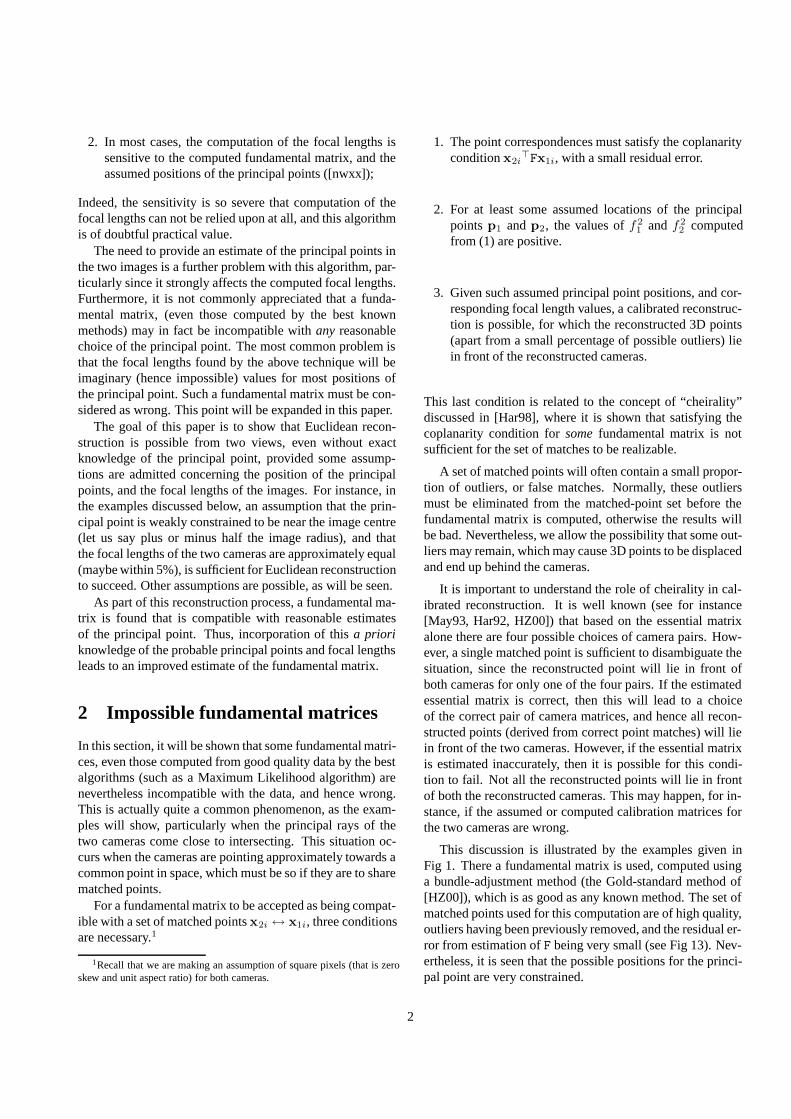
This discussion is illustrated by the examples given inFig 1. There a fundamental matrix is used, computed usinga bundle-adjustment method (the Gold-standard method of[HZ00]), which is as good as any known method. The set ofmatched points used for this computation are of high quality,outliers having been previously removed, and the residual er-ror from estimation of F being very small (see Fig 13). Nev-ertheless, it is seen that the possible positions for the princi-pal point are very constrained.

2

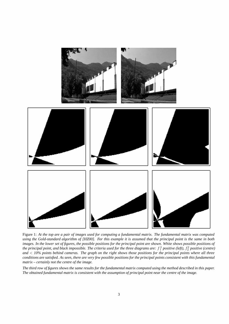
Figure 1: At the top are a pair of images used for computing a fundamental matrix. The fundamental matrix was computedusing the Gold-standard algorithm of [HZ00]. For this example it is assumed that the principal point is the same in bothimages. In the lower set of figures, the possible positions for the principal point are shown. White shows possible positions ofthe principal point, and black impossible. The criteria used for the three diagrams are: f 2

1 positive (left), f 22 positive (centre)

and < 10% points behind cameras. The graph on the right shows those positions for the principal points where all threeconditions are satisfied. As seen, there are very few possible positions for the principal points consistent with this fundamentalmatrix – certainly not the centre of the image.

The third row of figures shows the same results for the fundamental matrix computed using the method described in this paper.The obtained fundamental matrix is consistent with the assumption of principal point near the centre of the image.

3

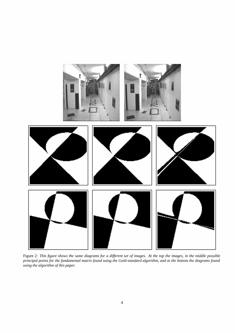
Figure 2: This figure shows the same diagrams for a different set of images. At the top the images, in the middle possibleprincipal points for the fundamental matrix found using the Gold-standard algorithm, and at the bottom the diagrams foundusing the algorithm of this paper.

4

Figure 3: This figure shows the possible principal point positions compatible with fundamental matrices computed using sev-eral different methods. The methods used are (from left to right, top to bottom) : normalized 8-point algorithm, gold-standardalgorithm, algebraic distance algorithm, Sampson-error algorithm, algorithm of this paper, and calibrated reconstructionalgorithm (see text for description).

5

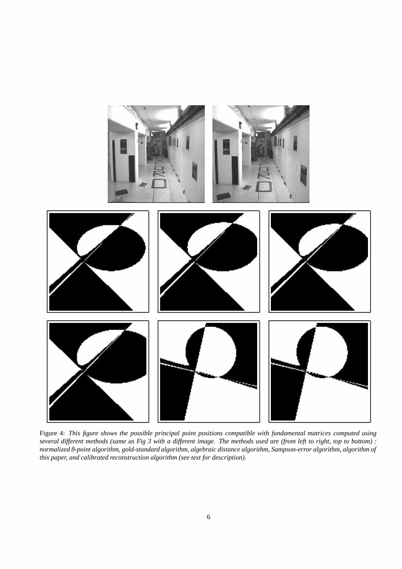
Figure 4: This figure shows the possible principal point positions compatible with fundamental matrices computed usingseveral different methods (same as Fig 3 with a different image. The methods used are (from left to right, top to bottom) :normalized 8-point algorithm, gold-standard algorithm, algebraic distance algorithm, Sampson-error algorithm, algorithm ofthis paper, and calibrated reconstruction algorithm (see text for description).

6

3 Using a priori knowledge to com-pute the fundamental matrix

It is often said that the computation of the fundamental ma-trix is unstable, and to an extent this is true. This is a charac-teristic of the problem itself, and not the algorithms used,since many algorithms that obtain close to the MaximumLikelihood estimate are known.

The fundamental matrix is however basically a projectiveobject, suitable for applying in situations where the cam-era calibration is unknown. However, it has been used inmany situations in which partial calibration of the camera isknown, at least approximately. There are many examples ofthis.

1. In reconstruction from two views, the camera calibra-tion is usually not completely unknown. For instance,the pixels are usually square, or at least rectangular withknown aspect ratio. The principal point is usually nearthe centre of the image, and the focal length is at leastknown within some reasonable bounds. In addition theprojective reconstruction algorithm based on the funda-mental matrix has been used in cases where the cali-bration of the camera is known. Oliensis [Oli00] hasundertaken a study of this, and argues that sometimescalibrated camera algorithms give better results.

2. The fundamental matrix has been used in self-calibration from two views ([Bou98, Har92]). To dothis, it is necessary to assume square pixels, and tomake an estimate of the principal point in the two im-ages. Unfortunately, the estimate of the focal lengthsis quite strongly dependent on the assumed locations ofthe principal points.

In this paper, we concentrate particularly on this secondscenario, in which the focal lengths of the cameras may becomputed from the fundamental matrix. However, we are in-terested in the inverse problem of using a priori estimates ofthe focal lengths of the cameras and also the principal pointsto improve the estimate of the fundamental matrix, and hencethe 3D reconstruction. This method, therefore lies betweentwo extremes – computation of the fundamental matrix fortotally uncalibrated cameras, and for completely calibratedcameras (in which case it is the essential matrix that is com-puted). In this case, we compute the fundamental matrixfor the case where the camera calibration is approximatelyknow.

A simple formula for the focal lengths, given the funda-mental matrix and principal point has been given by Boug-noux ([Bou98]):

f22 = − (p1

�[e1]×IF�p2)(p1�F�p2)

p1�([e1]×IF�IF)p1

(1)

where I is the diagonal matrix diag(1, 1, 0). A similar for-mula for f 2

1 is obtained by interchanging the roles of the twoimages.

However, this method has an important failure configu-ration, when the principal rays of the two cameras meet inspace ([NHBP96]). In this case, the principal points of thetwo cameras satisfy the coplanarity constraint p2

�Fp1 = 0.For many image pairs this condition is nearly satisfied. Thus,being close to a critical configuration, one might expect thatthe results will be quite unstable. A stability analysis forestimation of f in this instance was undertaken in [nwxx],in which it was verified that focal length estimate is indeedoften unreliable. It will be shown here that for many im-age pairs, the estimates of the focal length are effectivelyuseless. Worse, the algorithm often fails entirely. This is be-cause the formula of Bougnoux gives an expression for f 2

1 orf2

2 , the squares of the focal lengths of the two images. In thepresence of noise, or an inaccurate estimate of the principalpoint, the value of f 2 so obtained is negative, and so f is animaginary (hence impossible) value. Note that this is intrin-sic to the problem as formulated, and is not just an artefactof Bougnoux’s formula. In this failure case, the given funda-mental matrix is just not compatible with the assumed valuesof the two principal points. Either the fundamental matrix orthe principal point assumption is wrong.

The idea of this paper is to take advantage of this fact toobtain a better estimate of the fundamental matrix, and atthe same time a better estimate of the focal lengths of thecameras. The way this is done is to add additional termsin a cost function used to estimate F. These weight termsdiscriminate against improbable, or impossible values of theprincipal points of focal lengths of the cameras. Thus, a verysmall, or (worse) negative value of f 2 incurs a high cost,which makes it very unlikely to be accepted. If the weightsare related to a probability distribution for principal point orfocal length, then the new estimate of F may be thought ofas a maximum a priori (MAP) estimate of the fundamentalmatrix.

4 A cost function

Given a set of point correspondences x2i ↔ x1i, our ob-ject is to estimate the fundamental matrix subject to priorassumptions about the distribution of the focal lengths andprincipal points of the two cameras. The method is applica-ble easily to any assumed distributions, but most commonlya normal (Gaussian) distribution will be assumed. An iter-ative (Levenberg-Marquardt) method is used to minimize acost function of the following form:

Cost(F, f21 , f

22 ,p1,p2) = CF(F)+Cf (f2

1 , f22 )+Cp(p1,p2) .

(2)

7

Thus the total cost is the sum of three cost functions, mea-suring the cost of estimates of the fundamental matrix F, thesquared focal lengths f 2

1 and f 22 , and the principal points re-

spectively. The reason for expressing the second cost func-tion in terms of the squared focal lengths is because of theform of Bougnoux’s formula (1), as will be seen later. Wewant to define a cost (very high) for a negative value of f 2.

The cost functionCF(F) is also a function of the point cor-respondences. Although various cost functions are possible,we prefer to use the Sampson cost function

∑i

(x2i�Fx1i)2

(Fx1i)21 + (Fx1i)2

2 + (F�x2i)21 + (F�x2i)2

2

. (3)

This cost function is a first-order approximation to the cor-rect geometric (or Maximum Likelihood) cost function.

This cost function is minimized over a set of parametersby a parameter-minimization algorithm (LM). The set of pa-rameters is divided into two parts.

1. A set of parameters parametrizing the fundamental ma-trix F, and

2. A set of 4 (or 2) parameters defining the positions ofthe principal points. Two parameters may be used if itis assumed (and enforced) that the principal point is thesame in both images.

The minimization algorithm is as follows.

1. Given F and pi, compute f 21 and f 2

2 using Bougnoux’sformula (1).

2. Compute the cost function Cost(F, f 2i ,p

2i ).

3. Vary the parameters of F and the pi to minimize the costfunction.

Form of Cp and Cf . The specific form of the cost func-tions for pi and f 2

i may be chosen in various ways, and itis not the purpose of this paper to undertake a detailed in-vestigation of all possible cost functions. However, a naturalform for Cp is the squared Euclidean distance of the esti-mated principal point from the nominal value. Thus

Cp(pi) = w2pd(pi, pi)2 (4)

where pi) represents the nominal position of the principalpoint, and wp is a weight. There is a cost term of this formfor each of the two principal points.

The form of the cost function Cf may be a little morecomplicated, since we want to ensure that the value of f 2

does not end up negative. In addition, it may be appropri-ate to enforce a condition that the two focal lengths are thesame (or approximately so). Accordingly, the cost function

Cf (f21 , f

22 ) used in our implementation of the algorithm has

several components:

Cf (f21 , f2

2 ) = w21(f2

1 − f21 )2 + w2

2(f22 − f2

2 )2

+ w2d(f2

1 − f22 )

+ w2z1(f2

min − f21 )2 + w2

z2(f2min − f

22 )2 (5)

Recall here that f 2i is the value returned by Bougnoux’s

formula (1), and may be negative. The final two terms ofthis equation involve a “minimum” value fmin for the fo-cal length, and are only included if f 2

i < f2min. (That is

wz1 and wz2 are zero unless f 2i is small, or negative.). This

term grows rapidly for small or negative values of f 2i , and

effectively prevent f 2i taking on negative values. A reason-

able minimum value of fmin can be deduced from the sizeof the image. The field of view of the camera is equal to2 arctan(dim/f), where dim is the radius of the image. Forsmall values of f , this becomes unrealistically large. Mostimages encountered (except for extreme wide angled views)do not have field of view exceeding 75◦.

The choice of the weight values may be chosen accordingto taste. The values of wzi are not critical, and normally it issufficient to apply quite weak weights for the other values.

5 Initialization

The input data for the reconstruction problem includes an es-timate of the focal length and principal point of the cameras.Therefore, it makes sense to use these estimates to carry outa calibrated reconstruction to obtain an initial estimate of thefundamental matrix.

Thus, given a set of point correspondences, x2i ↔ x1i

and initial estimates pi and fi of the principal points andfocal lengths, an initial value for the fundamental matrix isfound as follows. Let K1 and K2 be the initial calibrationmatrices for the two images. Thus,

K1 =

f1 0 x1

f1 y1

1

K2 =

f2 0 x2

f2 y2

1

(6)

where pi = (xi, yi) are the principal points. Let F be an esti-mate of the fundamental matrix computed from the point cor-respondences using any desired method. We used a method([HZ00]) that minimizes algebraic error. The essential ma-trix E may then be computed as

E = K2�FK1 .

This value of the essential matrix will not generally be quitecorrect for the assumed calibration matrices, since it will notsatisfy the necessary condition for a essential matrix, namelythat it have two equal singular values. To correct this, the

8

singular value decomposition of E is computed as E = UDV�,and a corrected essential matrix is computed, by setting E =UIV�, where I = diag(1, 1, 0). Finally a corrected value ofthe fundamental matrix is computed by setting

F = K2−�EK−1

1 .

The resulting fundamental matrix F is the best approximationto F, compatible with the assumed calibration matrices.

Iteration will start with this estimate F for the fundamen-tal matrix, and the assumed values p1 and p2 for the twoprincipal points. The cost function CF(F) will be slightlygreater thanCF(F), but usually the difference is not too great.However, because of the way F is defined, the cost func-tions Cp(p1, p2) and Cf (f2

1 , f22 ) will both have initial val-

ues zero.The alternative is to start iteration with fundamental ma-

trix F, and the two principal point estimates. In this case,CF(F) will have a smaller value than CF(F), but the value ofCf (f2

1 , f22 ) will often be quite high, particularly if the values

of f 21 or f 2

2 are negative. Thus, the initial cost can be veryhigh, and we are starting far from the minimum. This canlead to problems with correct convergence.

Notice the difference between the two initial methods.Recall that the values of f 2

1 and f 22 are derived from the for-

mula (1) from the current (in this case the initial) estimatesof F and pi. Since F is a correct fundamental matrix for thecalibration matrices given in (6), it follows that (1) appliedto F and pi will give values of f 2

i = f2i , and so the cost

will be zero. However, (1) applied to F and the initial valuesof pi can give values of f 2

i that differ very greatly from thenominal values f2

i .

6 Experiments

The algorithm was carried out on both synthetic and realdata. The algorithms used for computing the fundamentalmatrix were as follows. For details of these algorithms, thereader is referred to [HZ00].

1. A normalized 8-point algorithm.

2. The gold-standard algorithm (bundle adjustment).

3. Iterative minimization of algebraic error (algebraic min-imization algorithm).

4. Iterative minimization of Sampson error, (3).

5. The algorithm of this paper (denoted by a-priori in thegraphs and tables).

6. Calibrated reconstruction, given fixed assumed valuesof the principal points and focal length.

The final algorithm is the one described in section 5,which is used as an initial point for the a-priori algorithm.

6.1 Synthetic image experiments

Evaluation of the method was carried out on two sets of data.In the first set, a set of scattered points on the surface of acube were used, and data were generated by projecting thepoints into a pair of nominal cameras. In the second set, apair of images were used to build a realistic-looking modelof a house (using the images in Fig 8). The model was thenprojected back into two images, approximating the originalimages. This data was the synthetic data, corresponding to arealistic imaging setup, that was used for experiments.

For each synthetic data set, noise was added in varyingdegrees, and Euclidean reconstruction was carried out. Theresults are shown in figures 5 – 7, which give the reconstruc-tion errors in each case.

The experiments were carried out with two different a-priori estimates for the principal point and focal length. Inthe first set, the exact values were given. This of coursegives a significant advantage to the calibrated reconstructionalgorithm, since it is provided with exact values for these pa-rameters. In the second set of experiments, the value of theprincipal point is shifted by 30 pixels in each dimension (in a512×512 image), and a slightly modified value for the focallength is given. This is perhaps more realistic, since theseparameter values may not be known exactly in advance.

Choice of weights. The a-priori algorithm was run withvery weak weights, in order to place minimal constraints onprincipal point and focal length. The value of wp was equalto 0.01, which means that a variation of 100 pixels (in a512 × 512 image) was given as much weight as one pixelreprojection error for a single matched point. The principalpoint was, however, assumed to be the same in both images.

As for the focal length, the weights w1 and w2 were setto zero, which means that no constraint was placed on theseparameters individually. However, a value of 0.001 was cho-sen for wd. This means that a value of 1000 for f 2

1 − f22

was equivalent to one pixel reprojection error. Since f i wasaround 500, this means approximately 2 pixels differencef1 − f2.

As stated, the values of wzi are not very critical. A valueof fmin = 100 was taken, and a weight wzi = 0.01 waschosen.

Findings. Perhaps because of the controlled nature of thesynthetic algorithms, in no case did the values of f 2

i turn outto be negative. As a result, the reconstruction results weregood for all the algorithms used. The a-priori algorithm per-formed significantly better than the calibrated reconstructionalgorithm, except in the case where exact parameters weregiven, and for high noise values.

9

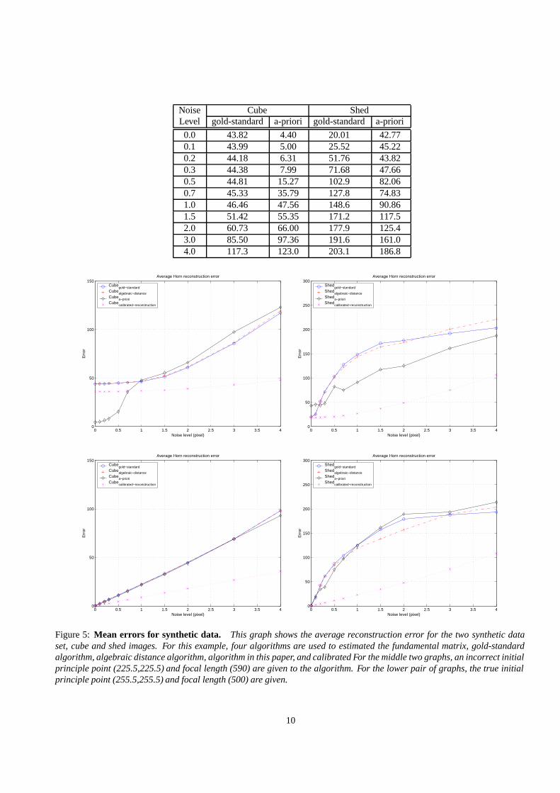
Noise Cube ShedLevel gold-standard a-priori gold-standard a-priori

0.0 43.82 4.40 20.01 42.770.1 43.99 5.00 25.52 45.220.2 44.18 6.31 51.76 43.820.3 44.38 7.99 71.68 47.660.5 44.81 15.27 102.9 82.060.7 45.33 35.79 127.8 74.831.0 46.46 47.56 148.6 90.861.5 51.42 55.35 171.2 117.52.0 60.73 66.00 177.9 125.43.0 85.50 97.36 191.6 161.04.0 117.3 123.0 203.1 186.8

0 0.5 1 1.5 2 2.5 3 3.5 40

50

100

150

Noise level (pixel)

Err

or

Average Horn reconstruction error

Cubegold−standard

Cubealgebraic−distance

Cubea−priori

Cubecalibrated−reconstruction

0 0.5 1 1.5 2 2.5 3 3.5 40

50

100

150

200

250

300

Noise level (pixel)

Err

or

Average Horn reconstruction error

Shedgold−standard

Shedalgebraic−distance

Sheda−priori

Shedcalibrated−reconstruction

0 0.5 1 1.5 2 2.5 3 3.5 40

50

100

150

Noise level (pixel)

Err

or

Average Horn reconstruction error

Cubegold−standard

Cubealgebraic−distance

Cubea−priori

Cubecalibrated−reconstruction

0 0.5 1 1.5 2 2.5 3 3.5 40

50

100

150

200

250

300

Noise level (pixel)

Err

or

Average Horn reconstruction error

Shedgold−standard

Shedalgebraic−distance

Sheda−priori

Shedcalibrated−reconstruction

Figure 5: Mean errors for synthetic data. This graph shows the average reconstruction error for the two synthetic dataset, cube and shed images. For this example, four algorithms are used to estimated the fundamental matrix, gold-standardalgorithm, algebraic distance algorithm, algorithm in this paper, and calibrated For the middle two graphs, an incorrect initialprinciple point (225.5,225.5) and focal length (590) are given to the algorithm. For the lower pair of graphs, the true initialprinciple point (255.5,255.5) and focal length (500) are given.

10

Noise Cube ShedLevel gold-standard a-priori gold-standard a-priori

0.0 43.82 4.40 20.01 42.770.1 43.12 4.47 22.38 42.460.2 42.40 5.42 37.28 43.820.3 41.70 6.40 57.84 43.010.5 40.27 10.19 93.17 39.740.7 38.88 14.98 166.8 37.071.0 37.00 23.44 168.2 43.781.5 34.49 33.98 170.234 59.212.0 35.88 43.62 169.6 60.83.0 68.46 76.68 170.7 131.24.0 111.0 86.18 172.7 187.8

0 0.5 1 1.5 2 2.5 3 3.5 40

50

100

150

Noise level (pixel)

Err

or

Median Horn reconstruction error

Cubegold−standard

Cubealgebraic−distance

Cubea−priori

Cubecalibrated−reconstruction

0 0.5 1 1.5 2 2.5 3 3.5 40

50

100

150

200

250

300

Noise level (pixel)

Err

or

Median Horn reconstruction error

Shedgold−standard

Shedalgebraic−distance

Sheda−priori

Shedcalibrated−reconstruction

0 0.5 1 1.5 2 2.5 3 3.5 40

50

100

150

Noise level (pixel)

Err

or

Median Horn reconstruction error

Cubegold−standard

Cubealgebraic−distance

Cubea−priori

Cubecalibrated−reconstruction

0 0.5 1 1.5 2 2.5 3 3.5 40

50

100

150

200

250

300

Noise level (pixel)

Err

or

Median Horn reconstruction error

Shedgold−standard

Shedalgebraic−distance

Sheda−priori

Shedcalibrated−reconstruction

Figure 6: Median errors for synthetic data. This gives the same results as in Fig 5 except that median error is given, insteadof average.

11

Figure 7: Reconstructed models. This figure shows the reconstruction result of the synthetic shed images derived from theimages in Fig 8. On the top row, a reconstruction from noise-free data is shown. On the second row a reconstruction using thegold-standard algorithm for noise levels of 0.4, 1.0 and 2.0 pixels (left to right). The third row shows the recontruction withalgebraic distance algorithm. The last row shows the reconstruction with the algorithm in this paper.

12

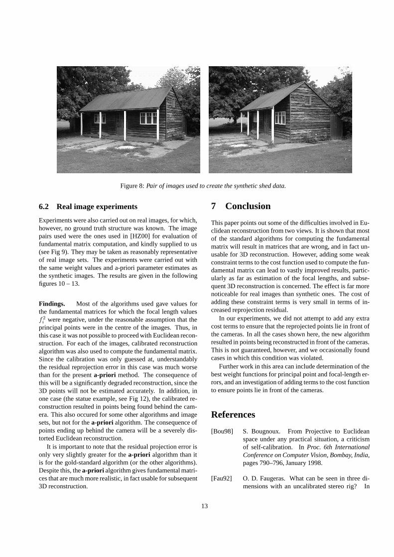
Figure 8: Pair of images used to create the synthetic shed data.

6.2 Real image experiments

Experiments were also carried out on real images, for which,however, no ground truth structure was known. The imagepairs used were the ones used in [HZ00] for evaluation offundamental matrix computation, and kindly supplied to us(see Fig 9). They may be taken as reasonably representativeof real image sets. The experiments were carried out withthe same weight values and a-priori parameter estimates asthe synthetic images. The results are given in the followingfigures 10 – 13.

Findings. Most of the algorithms used gave values forthe fundamental matrices for which the focal length valuesf2i were negative, under the reasonable assumption that the

principal points were in the centre of the images. Thus, inthis case it was not possible to proceed with Euclidean recon-struction. For each of the images, calibrated reconstructionalgorithm was also used to compute the fundamental matrix.Since the calibration was only guessed at, understandablythe residual reprojection error in this case was much worsethan for the present a-priori method. The consequence ofthis will be a significantly degraded reconstruction, since the3D points will not be estimated accurately. In addition, inone case (the statue example, see Fig 12), the calibrated re-construction resulted in points being found behind the cam-era. This also occured for some other algorithms and imagesets, but not for the a-priori algorithm. The consequence ofpoints ending up behind the camera will be a severely dis-torted Euclidean reconstruction.

It is important to note that the residual projection error isonly very slightly greater for the a-priori algorithm than itis for the gold-standard algorithm (or the other algorithms).Despite this, the a-priori algorithm gives fundamental matri-ces that are much more realistic, in fact usable for subsequent3D reconstruction.

7 Conclusion

This paper points out some of the difficulties involved in Eu-clidean reconstruction from two views. It is shown that mostof the standard algorithms for computing the fundamentalmatrix will result in matrices that are wrong, and in fact un-usable for 3D reconstruction. However, adding some weakconstraint terms to the cost function used to compute the fun-damental matrix can lead to vastly improved results, partic-ularly as far as estimation of the focal lengths, and subse-quent 3D reconstruction is concerned. The effect is far morenoticeable for real images than synthetic ones. The cost ofadding these constraint terms is very small in terms of in-creased reprojection residual.

In our experiments, we did not attempt to add any extracost terms to ensure that the reprojected points lie in front ofthe cameras. In all the cases shown here, the new algorithmresulted in points being reconstructed in front of the cameras.This is not guaranteed, however, and we occasionally foundcases in which this condition was violated.

Further work in this area can include determination of thebest weight functions for principal point and focal-length er-rors, and an investigation of adding terms to the cost functionto ensure points lie in front of the cameras.

References

[Bou98] S. Bougnoux. From Projective to Euclideanspace under any practical situation, a criticismof self-calibration. In Proc. 6th InternationalConference on Computer Vision, Bombay, India,pages 790–796, January 1998.

[Fau92] O. D. Faugeras. What can be seen in three di-mensions with an uncalibrated stereo rig? In

13

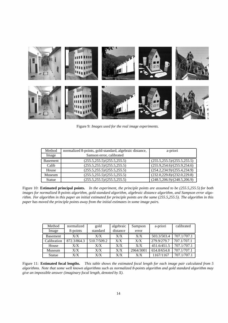
Figure 9: Images used for the real image experiments.

Method normalized 8-points, gold-standard, algebraic distance, a-prioriImage Samson error, calibrated

Basement (255.5,255.5)/(255.5,255.5) (255.5,255.5)/(255.5,255.5)Calib (255.5,255.5)/(255.5,255.5) (255.9,254.6)/(255.9,254.6)House (255.5,255.5)/(255.5,255.5) (254.2,234.9)/(255.4,234.9)

Museum (255.5,255.5)/(255.5,255.5) (232.0,229.8)/(232.0,229.8)Statue (255.5,255.5)/(255.5,255.5) (248.5,206.9)/(248.5,206.9)

Figure 10: Estimated principal points. In the experiment, the principle points are assumed to be (255.5,255.5) for bothimages for normalized 8-points algorithm, gold-standard algorithm, algebraic distance algorithm, and Sampson error algo-rithm. For algorithm in this paper an initial estimated for principle points are the same (255.5,255.5). The algorithm in thispaper has moved the principle points away from the initial estimates in some image pairs.

Method normalized gold algebraic Sampson a-priori calibratedImage 8-points standard distance error

Basement X/X X/X X/X X/X 503.3/503.4 707.1/707.1Calibration 872.3/864.3 510.7/509.2 X/X X/X 279.9/279.7 707.1/707.1

House X/X X/X X/X X/X 451.6/451.5 707.1/707.1Museum X/X X/X X/X 2964/3001 654.8/654.8 707.1/707.1

Statue X/X X/X X/X X/X 1167/1167 707.1/707.1

Figure 11: Estimated focal lengths. This table shows the estimated focal length for each image pair calculated from 5algorithms. Note that some well known algorithms such as normalized 8-points algorithm and gold standard algorithm maygive an impossible answer (imaginary focal length, denoted by X).

14

Method normalized gold algebraic Sampson a-priori calibratedImage 8-points standard distance error

Basement 0/0 0/0 0/100 0/0 100/100 100/100Calibration 100/100 100/100 100/0 100/100 100/100 100/100

House 91.7/91.7 100/0 100/0 100/0 100/100 100/100Museum 0/0 0/100 0/100 94.9/94.9 100/100 100/100

Statue 100/100 100/0 100/0 100/100 100/100 52.4/52.4

Figure 12: Percentage points in front of cameras. This table shows the percentage of points that lie in front of eachcamera in each image pair. It is clear that the algorithm in this paper gives a better result in that the estimated fundamentalmatrix yields estimated points in front of the camera. When wrong principle points and focal length are used in the calibratedreconstruction algorithm some points may end up behind the cameras, as seen for the statue pair.

1 2 3 4 50

0.2

0.4

0.6

0.8

1

1.2

1.4

Image: 1/Basement, 2/Calibration, 3/House, 4/Museum, 5/Statue

Err

or

RMS error

normalized 8−pointsgold−standardalgebraic distanceSampson−errora−prioricalibrated−reconstruction

Figure 13: Residuals. This figure summarizes the residual rms error of the estimated fundamental matrix obtained from 5algorithms: normalized 8-points algorithm, gold-standard algorithm, algebraic distance algorithm, Sampson error algorithm,algorithm in this paper, and algorithm in this paper with constraints on the focal length and principle point. It is clear thatthe algorithm in this paper gives a similar level of residual RMS error when compared with the other uncalibrated algorithms.However, using a calibrated reconstruction algorithm gives significantly higher residual, because the internal parameters maynot have been guessed correctly.

15

Proc. European Conference on Computer Vi-sion, LNCS 588, pages 563–578. Springer-Verlag, 1992.

[Har92] R. I. Hartley. Estimation of relative camera po-sitions for uncalibrated cameras. In Proc. Eu-ropean Conference on Computer Vision, LNCS588, pages 579–587. Springer-Verlag, 1992.

[Har98] R. I. Hartley. Chirality. International Journal ofComputer Vision, 26(1):41–61, 1998.

[HGC92] R. I. Hartley, R. Gupta, and T. Chang. Stereofrom uncalibrated cameras. In Proc. IEEE Con-ference on Computer Vision and Pattern Recog-nition, 1992.

[Hor90] B. K. P. Horn. Relative orientation. InternationalJournal of Computer Vision, 4:59–78, 1990.

[Hor91] B. K. P. Horn. Relative orientation revis-ited. Journal of the Optical Society of America,8(10):1630–1638, 1991.

[HZ00] R. I. Hartley and A. Zisserman. Multiple ViewGeometry in Computer Vision. Cambridge Uni-versity Press, 2000.

[LH81] H. C. Longuet-Higgins. A computer algorithmfor reconstructing a scene from two projections.Nature, 293:133–135, September 1981.

[May93] S. J. Maybank. Theory of reconstruction fromimage motion. Springer-Verlag, Berlin, 1993.

[NHBP96] G. Newsam, D. Q. Huynh, M. Brooks, and H. P.Pan. Recovering unknown focal lengths in self-calibration: An essentially linear algorithm anddegenerate configurations. In Int. Arch. Pho-togrammetry & Remote Sensing, volume XXXI-B3, pages 575–80, Vienna, 1996.

[nwxx] Author name withheld. Paper title withheld. Inxx, xx.

[Oli00] J. Oliensis. A critique of structure from motionalgorithms. Computer Vision and Image Under-standing, 80:172–214, 2000.

16