recap – shape functions - cleveland state universityacademic.csuohio.edu/duffy_s/cve_512_...

Section 11: ISOPARAMETRIC FORMULATION

Recap – Shape Functions

This is a good place to stop and remind ourselves where we are in the process ofThis is a good place to stop and remind ourselves where we are in the process of formulating numerical solutions using finite element methods. For a component we are solving the global force displacement equation

{ } [ ]{ }dKF =

for displacements, i.e.,

{ } [ ]{ }dKF =

{ } { }[ ] 1−= KFd

The key to doing this is formulating the global stiffness matrix [K] properly and finding its inverse. Once we have solved for the displacements AT THE NODES, we can interpolate

{ } { }[ ]= KFd

p , pdisplacements (u, v) across the element through the use of shape functions. For one dimensional line elements

− xxx dxxdNdNddd 112

ˆˆˆ1ˆˆˆ

ˆˆˆˆ

where the coordinate axis was attached to the left end of the element.

−=+=

+=x

xxx

xxx

dLLdNdNx

Ldu

2

12211

121 ˆ

,1


The linear shape functions for the one dimensional rod element are

xNˆ

11 −=xNˆ

2 =

relative to a local coordinate system attached to the left end. For a two dimensional constant strain triangle, once the nodal displacements were determined, the displacements

h l b i l d i h h h f h f i

LN 11 L

N2

across the element can be interpolated again through the use of shape functions

( ) mmjjii uNuNuNyxu ++=,

( ) vNvNvNyxv ++=and these shape functions are formulated using global coordinate axes (x, y). For the constant strain triangle the shape functions are linear in x and y, i.e.,

1

( ) mmjjii vNvNvNyxv ++=,

( )

( )yxA

N

yxA

N

jjjj

iiii

γβα

γβα

++

=

++

=

21

21

( )yxA

N

A

mmmm

jjjj

γβα ++

=

21

2


For the linear strain triangle element displacements were quadratic functions of position. Recall that

H ft th d l di l t d t i d ll th t th ffi i t b

( )( ) 2

12112

10987

265

24321

,

,

yaxyaxayaxaayxv

yaxyaxayaxaayxu

+++++=

+++++=

Here after the nodal displacements are determined recall that the coefficients above are determined through the following expression

{ } [ ] { }da 1−= χand the displacements are interpolated across the element using

{ }{ }aMvu

=

*

where now the shape functions are defined as

{ }[ ] { } { }{ }dNdM

v

==

−1* χ

{ } { }[ ] 1* −= χMN


For the linear strain triangle element the displacements vary quadratically across the element and the shape functions must be able to interpolate the nodal displacements

d i ll h l h f h h l blquadratically across the element. Thus for the the example problem

hy

bhxy

bx

hy

bxN 242331 2

2

2

2

1 +++−−=

bx

bxN

hbhbhb

2

2

2

2

2

2 +−= Note carefully that the shape functions are dependent upon a coordinate system whose origin was attached to the first corner node Change the

bhxyN

hy

hyN

4

2

4

23

=

+−=was attached to the first corner node. Change the coordinate system and the shape functions change.

Tracking the shape function for each individual element relative to a single coordinate system now

hy

bhxy

hyN

bh444

2

2

5

4

−−=

element relative to a single coordinate system now becomes problematic. This is not something one can do by hand or track easily in computer software.

bhxy

bx

bxN 444

2

2

6 −−= We will begin the use a local coordinate system as we formulate higher order elements.


Geometric InterpolationWe just reviewed how shape functions are used to interpolate nodal displacements across

l t d l di l t k O di l t d h than element – once nodal displacements were known. Once displacements and how they vary across the element are known, derivatives of displacement can be taken to obtain strain. Once strain is computed we compute stress across the element.

If the nodal coordinates are available we can perform the same sort of interpolation toIf the nodal coordinates are available we can perform the same sort of interpolation to define the curved boundary (geometry) of an element. Consider the classic problem of a plate with a hole subject to a tensile stress boundary condition. We could use quadrilateral elements with four corner nodes

But there is a loss in fidelity along the straight line edges of the elementline edges of the element.


We could develop a quadrilateral element with mid side nodes just as we did with triangular elements. The boundary between corner nodes could have a curved shape based on a quadratic interpolation of the coordinates of the corners and the mid side b sed o qu d c e po o o e coo d es o e co e s d e d s denode:

Note that the coordinates of nodes are specified and the software fits a curve through location of the nodes. Quadratic interpolation functions allows mid side nodes to be moved relative to corner nodes producing curved boundaries. This type of element have much more fidelity in modeling the geometry of this components.


The concepts are developed referencing the figures below and defining the mathematics going from left to right, i.e., from natural coordinates to global coordinates. However, inverses exist for these transformations such that one can define the geometry on the right hand side, transform the problem to the natural coordinates on the left hand side and perform calculations in the natural coordinate system. Calculations in the natural coordinate system are far easier. After a formal definition of isoparametric elements the mathematics associated with the mapping indicated below is presented

t

1 11t

with the mapping indicated below is presented.

s1 1

1s

y

xt

Natural Coordinates t

1y

tGlobal Coordinates

s1

y

xs


Isoparametric FormulationDeveloping shape functions and element stiffness matrices in terms of the global coordinate

t f hi h d l t i diffi lt I t i f l ti f fi it l tsystem for higher order elements is difficult. Isoparametric formulations for finite elements is a way around this complexity. In addition, the isoparametric formulation allows the development of elements that have curved sides.

A finite element is said to be isoparametric if the same interpolation functions define bothA finite element is said to be isoparametric if the same interpolation functions define both the displacement shape functions and the geometric shape functions. Geometric shape functions define the transformation used to go back and forth from an x-y coordinate system to an s-t coordinate system for two dimensional elements. If the geometric interpolation functions are of lower order than the displacement shape functions the element is said to be subparametric. If the reverse holds, then the element is referred to as superparametric.

Isoparametric elements have curved boundaries which make them more suitable in capturing geometric boundary conditions. For higher order elements it is necessary to employ numerical integration to evaluate the element stiffness matrix. Transformation to an s-tcoordinate system, a natural coordinate system, facilitates integration. The methods are a necessity for quadratic elements as well as higher order elements In commercial softwarenecessity for quadratic elements as well as higher order elements. In commercial software the isoparametric formulation is used for both low order and higher order elements.


F di i l l h l di i d fi d b l

Rectangular Plane Stress Element

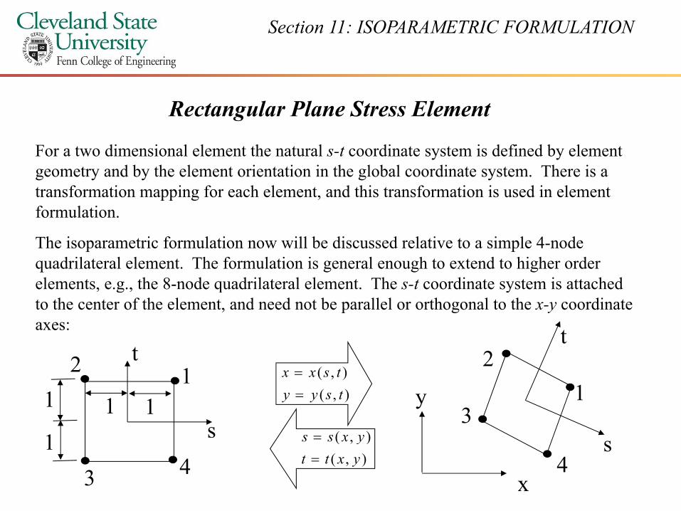
For a two dimensional element the natural s-t coordinate system is defined by element geometry and by the element orientation in the global coordinate system. There is a transformation mapping for each element, and this transformation is used in element formulation.

The isoparametric formulation now will be discussed relative to a simple 4-node quadrilateral element. The formulation is general enough to extend to higher order elements, e.g., the 8-node quadrilateral element. The s-t coordinate system is attached g q yto the center of the element, and need not be parallel or orthogonal to the x-y coordinate axes:

2 t 2t

2

s1 1

11

1

y 12

3),(),(

tsyytsxx

==

)( yxss =

3 41

4x

s),(),(

yxttyxss

==


This quadrilateral element has eight degrees of freedom, i.e., two displacements at each node. The unknown nodal displacements are defined as

1

1

vu

4y

3

{ }

=3

2

2

uvu

d xb bh

h

4

3

vuv 1 2

Here

4v

( ) xyayaxaayxu +++( )( ) xyayaxaayxv

xyayaxaayxu

8765

4321

,,

+++=+++=


If we solve for the coefficients in the usual manner the expressions for the displacements in the element are

( ) ( )( ) ( )( )

( )( ) ( )( ) ]

[41, 21

hbhb

uyhxbuyhxbbh

yxu −++−−=

( )( ) ( )( ) ]43 uyhxbuyhxb +−++++

( ) ( )( ) ( )( )[41, 21 vyhxbvyhxbbh

yxv −++−−=

or

( ) ( )( ) ( )( )

( )( ) ( )( ) ]

[4

43

21

vyhxbvyhxb

yybh

y

+−++++

( )( ) { }{ }dN

yxvyxu

=

,,


where

bhyhxbyxN

4))((),(1

−−=

yhxbbh

yhxbyxN

bh

))(()(

4))((),(

4

2

++

−+=

bhyhxbyxN

bhyhxbyxN

4))((),(

4))((),(

4

3

+−=

++=

uandbh4

2

1

1

uvu

=

3

3

2

4321

4321

00000000

vuv

NNNNNNNN

vu

4

4

3

vu


Again the element strains for this two dimensional element are

∂u

∂∂∂

=

yvx

y

x

εε

and

∂∂

+∂∂

xv

yuxyγ

and

{ } { }{ }dB=ε

The {B} matrix can be found by taking appropriate derivatives of the shape functions. The resulting expression for strain will demonstrate that the strain in the x-direction is only dependent on y, the strain in the y-direction is only dependent on x, and the shear strain is d d b h d ll i li f hidependent on both x and y, all in a linear fashion.


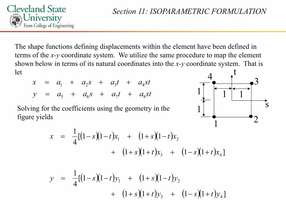
The shape functions defining displacements within the element have been defined in terms of the x-y coordinate system. We utilize the same procedure to map the element h b l i f i l di i h di h ishown below in terms of its natural coordinates into the x-y coordinate system. That is

letstatasaax 4321 +++=

4 t

1 13

1statasaay 8765 +++=

1

s1 1

2

1

1Solving for the coefficients using the geometry in the figure yields

1 2

( )( ) ( )( )

( )( ) ( )( ) ]1111

1111[41

21

xtsxts

xtsxtsx

+−++++

−++−−=

( )( ) ( )( ) ]1111 43 xtsxts +++++

( )( ) ( )( )1111[41

21 ytsytsy −++−−=

( )( ) ( )( ) ]11114

43 ytsyts +−++++


Or in matrix notation

1

1

yx

=

2

2

4321

00000000

xyx

NNNNNNNN

yx

where

4

3

34321 0000

xyxNNNNy

)1)(1(4

)1)(1(),(1tstsN −−

=

4y

)1)(1(),(

4)1)(1(),(

3

2

tstsN

tstsN

++=

−+=

4)1)(1(),(

4),(

4

3

tstsN +−=


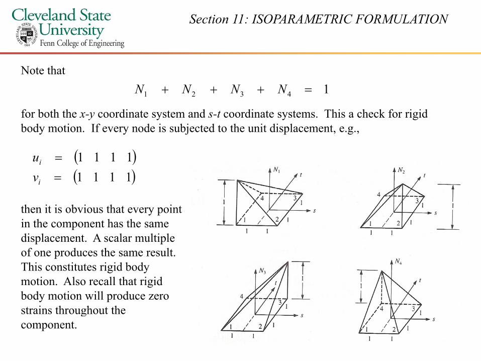
Note that14321 =+++ NNNN

for both the x-y coordinate system and s-t coordinate systems. This a check for rigid body motion. If every node is subjected to the unit displacement, e.g.,

( )1111( )( )1111

1111==

i

i

vu

th it i b i th t i tthen it is obvious that every point in the component has the same displacement. A scalar multiple of one produces the same result. pThis constitutes rigid body motion. Also recall that rigid body motion will produce zero strains throughout thestrains throughout the component.


We now turn our attention to formulating the {B} matrix for the quadrilateral element. This formulation could be carried out in the x-y coordinate system but the computations are difficult to nearly impossible. It is tedious to execute these computations in the s-tcoordinate system, but it is doable.

To construct the element stiffness matrix we must have expressions for strains which are theoretically derived in terms of derivatives of the displacements with respect to the x-ycoordinate system. If you use the s-t coordinate system to find displacements, the displacements are functions of s and t, and not x and y. Therefore we need to apply the chain rule for differentiation. This means the derivatives of the displacements are

yuxuusy

yu

sx

xu

su

∂∂+

∂∂=

∂∂∂

∂∂

+∂∂

∂∂

=∂∂

sy

yv

sx

xv

sv

tytxt

∂∂

∂∂

+∂∂

∂∂

=∂∂

∂∂+

∂∂=

∂

ty

yv

tx

xv

tv

sysxs

∂∂

∂∂

+∂∂

∂∂

=∂∂

∂∂∂∂∂


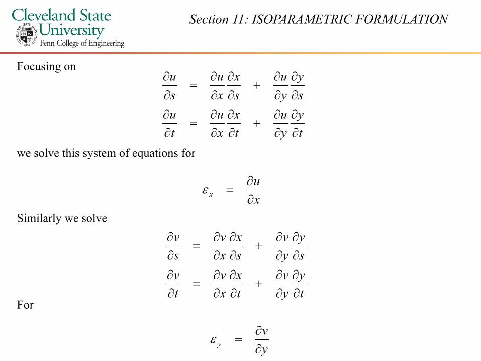
Focusing on

sy

yu

sx

xu

su

∂∂

∂∂

+∂∂

∂∂

=∂∂

we solve this system of equations for

ty

yu

tx

xu

tu

∂∂

∂∂

+∂∂

∂∂

=∂∂

we solve this system of equations for

xu

x ∂∂

=ε

Similarly we solve

sy

yv

sx

xv

sv

∂∂

∂∂

+∂∂

∂∂

=∂∂

Forty

yv

tx

xv

tv

sysxs

∂∂

∂∂

+∂∂

∂∂

=∂∂

∂∂∂∂∂

yv

y ∂∂

=ε


Using Cramer’s rule

yu ∂∂ vx ∂∂

ty

tu

sy

su

u ∂∂

∂∂

∂∂

∂∂

∂ tv

tx

sv

sx

v ∂∂

∂∂

∂∂

∂∂

∂

yxsy

sx

ttxx

∂∂∂∂

∂∂

∂∂=∂

=ε

yxsy

sx

ttyv

y

∂∂∂∂

∂∂

∂∂=∂∂

=ε

where the determinants in the denominator is the determinant of the Jacobian matrix, i.e.,

ty

tx

∂∂

∂∂

ty

tx

∂∂

∂∂

sy

sx

J ∂∂

∂∂

=

ty

tx

J

∂∂

∂∂

=


For the shear strainyvux ∂∂∂∂

ty

tv

ss

tu

tx

ss

vuxy ∂∂

∂∂

∂∂

∂∂

+∂∂∂∂

∂∂

∂∂

=∂∂

+∂∂

=γ

yxsy

sx

yxsy

sxxyxy

∂∂

∂∂

∂∂

∂∂

∂∂

∂∂

∂∂

∂∂∂∂

γ

These determinant expressions lead totttt ∂∂∂∂

∂∂∂∂∂ uyuyu 1

∂∂

∂∂

−∂∂

∂∂

=∂∂

=tu

sy

su

ty

Jxu

x1ε

∂∂∂∂∂ vxvxv 1

∂∂

∂∂

−∂∂

∂∂

=∂∂

=sv

tx

tv

sx

Jyv

y1ε


and

∂∂ vu

∂∂

∂∂

−∂∂

∂∂

+∂∂

∂∂

−∂∂

∂∂

=

∂∂

+∂∂

=

vyvyuxxuJ

xv

yu

xy

1

γ

In a matrix format

∂∂∂∂∂∂∂∂ tsstststJ

∂∂∂∂∂∂

∂∂

−∂∂

∂∂

=

∂∂∂

=

uxx

tsy

sty

vxu

x

0

0

1εε

∂∂

∂∂

−∂∂

∂∂

∂∂

∂∂

−∂∂

∂∂

∂∂−

∂∂=

∂∂

+∂∂∂

=

v

tsy

sty

stx

tsx

sttsJ

yv

xu

yxy

y 0

γ

ε

y


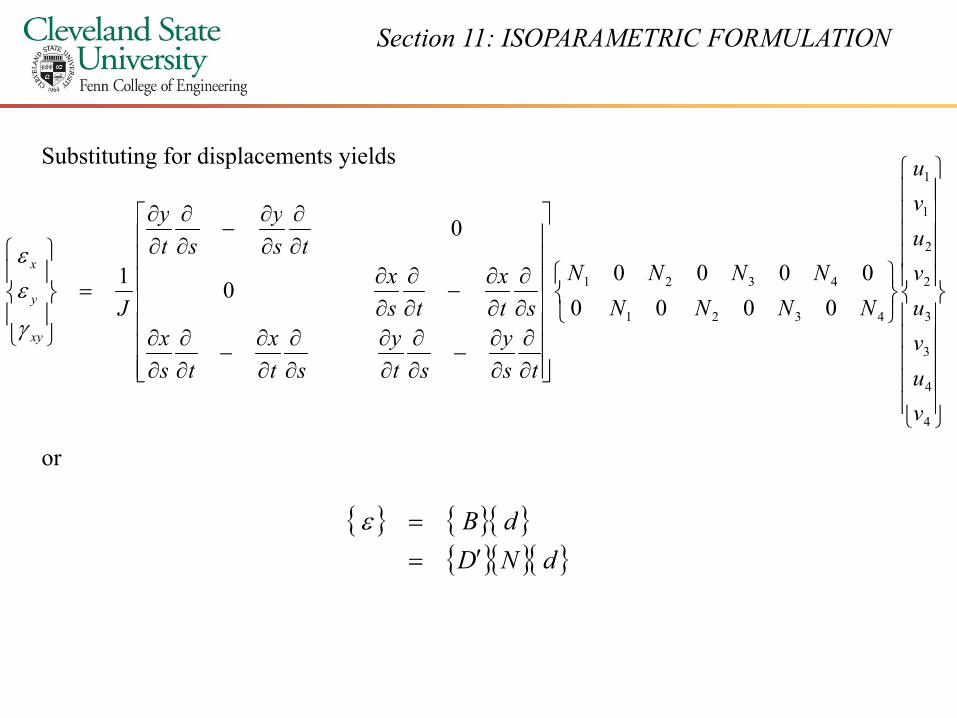
Substituting for displacements yields

∂∂∂∂

1

vu

∂∂

∂∂

−∂∂

∂∂

∂∂

∂∂

−∂∂

∂∂

=

2

2

1

4321

00000000

0

0

1uvuv

NNNNNNNN

stx

tsx

tsy

sty

Jy

x

εε

∂∂

∂∂

−∂∂

∂∂

∂∂

∂∂

−∂∂

∂∂

∂∂∂∂

4

3

34321 0000

vuvuNNNN

tsy

sty

stx

tsx

sttsJxyγ

or

4v

{ } { }{ }dB{ } { }{ }{ }{ }{ }dND

dB′=

=ε


where we define the operator matrix

∂∂

∂∂

−∂∂

∂∂

tsy

sty 0

{ }

∂∂

∂∂

−∂∂

∂∂

∂∂

∂∂

−∂∂

∂∂

∂∂

∂∂

−∂∂

∂∂

=′

yyxxst

xts

xJ

D 01

The matrix {B} is now expressed as a function of s and t, i.e., ∂∂∂∂∂∂∂∂ tsststts

∂∂

−∂∂ 0yy

{ }

∂∂∂∂∂∂∂∂∂∂

∂∂

−∂∂

∂∂

∂∂∂∂

=4321

4321

00000000

0

0

1NNNN

NNNNst

xts

xtsst

JB

but because of J, the variables s and t appear in the numerator and the denominator of the

∂

∂∂∂

−∂∂

∂∂

∂∂

∂∂

−∂∂

∂∂

tsy

sty

stx

tsx

components of the {B} matrix. This complicates integration to obtain the element stiffness matrix (refer to your Calculus text books for the integration of rational polynomials).


A final note on computing the determinant of the Jacobian matrix. With

xtsNx )(∑=

ii

i

ii

i

ytsNy

xtsNx

),(

),(

∑

∑=

=

then

∑ ∂∂

=∂∂

ii

i xs

tsNsx ),(

and

∑ ∂∂

=∂∂

ii

i xt

tsNtx ),(

∑∂∂

∂∂

=∂∂

ii

i

N

ys

tsNsy

)(

),(

∑ ∂∂

=∂∂

ii

i yt

tsNty ),(


∂∂ yx

This leads to

[ ]

∂∂

∂∂

∂∂=

ty

tx

ssJ

∂∂∂

∂∂

∂

=∑∑

∑∑ii

ii

i

ii

i

ytsNxtsN

ys

tsNxs

tsN

),(),(

),(),(

∂∂ ∑∑

ii

ii y

tx

t

thus

∂

∂

∂

∂

∂

∂=

∑∑

∑∑i

ii

ii

i

tsNtsN

yt

tsNxs

tsNJ

)()(

),(),(

∂

∂

∂

∂− ∑∑

ii

i

ii

i ys

tsNxt

tsN ),(),(


I l lIn class example


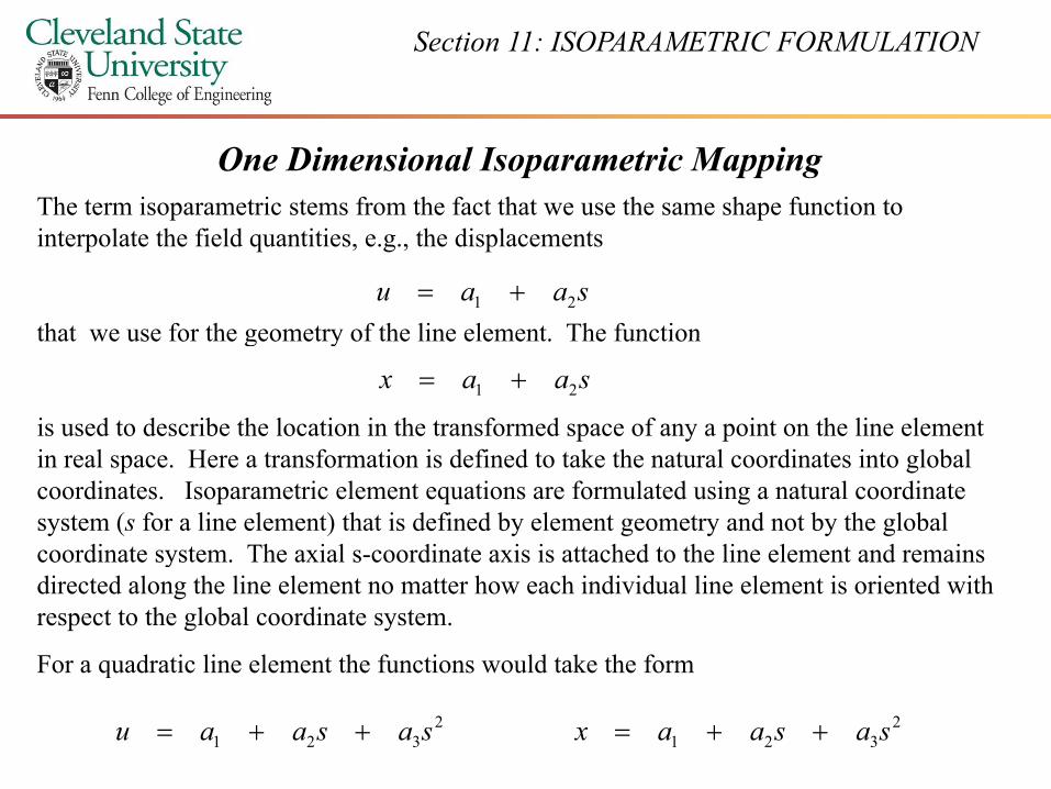
One Dimensional Isoparametric MappingThe term isoparametric stems from the fact that we use the same shape function to interpolate the field quantities, e.g., the displacements

that we use for the geometry of the line element The functionsaau 21 +=

that we use for the geometry of the line element. The function

is used to describe the location in the transformed space of any a point on the line element i l H f i i d fi d k h l di i l b l

saax 21 +=

in real space. Here a transformation is defined to take the natural coordinates into global coordinates. Isoparametric element equations are formulated using a natural coordinate system (s for a line element) that is defined by element geometry and not by the global coordinate system. The axial s-coordinate axis is attached to the line element and remains ydirected along the line element no matter how each individual line element is oriented with respect to the global coordinate system.

For a quadratic line element the functions would take the formq

2321 sasaau ++= 2

321 sasaax ++=


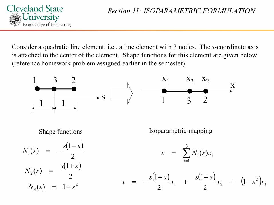
Consider a quadratic line element, i.e., a line element with 3 nodes. The s-coordinate axis is attached to the center of the element. Shape functions for this element are given below

x2x1 x1 2

p g(reference homework problem assigned earlier in the semester)

3 x3

1 2s1 1 3

`

Shape functions

( )1 ss −

Isoparametric mapping

3( )

( )2

1

21)(

21)(

sssN

sssN

+=

−−= ∑

=

=3

1)(

iii xsNx

( ) ( )11 +2

3 1)(2ssN −=

( ) ( ) ( ) 32

21 12

12

1 xsxssxssx −++

+−

−=


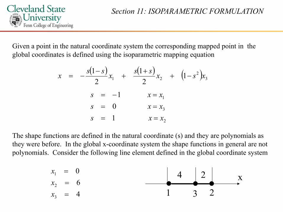
Given a point in the natural coordinate system the corresponding mapped point in the global coordinates is defined using the isoparametric mapping equation

( ) ( ) ( ) 32

21 12

12

1 xsxssxssx −++

+−

−=

2

3

1

10

1

xxsxxsxxs

=====−=

2

The shape functions are defined in the natural coordinate (s) and they are polynomials as they were before. In the global x-coordinate system the shape functions in general are not

l i l C id th f ll i li l t d fi d i th l b l di t tpolynomials. Consider the following line element defined in the global coordinate system

601 =

xx

x4 2

46

3

2

==

xx

1 23


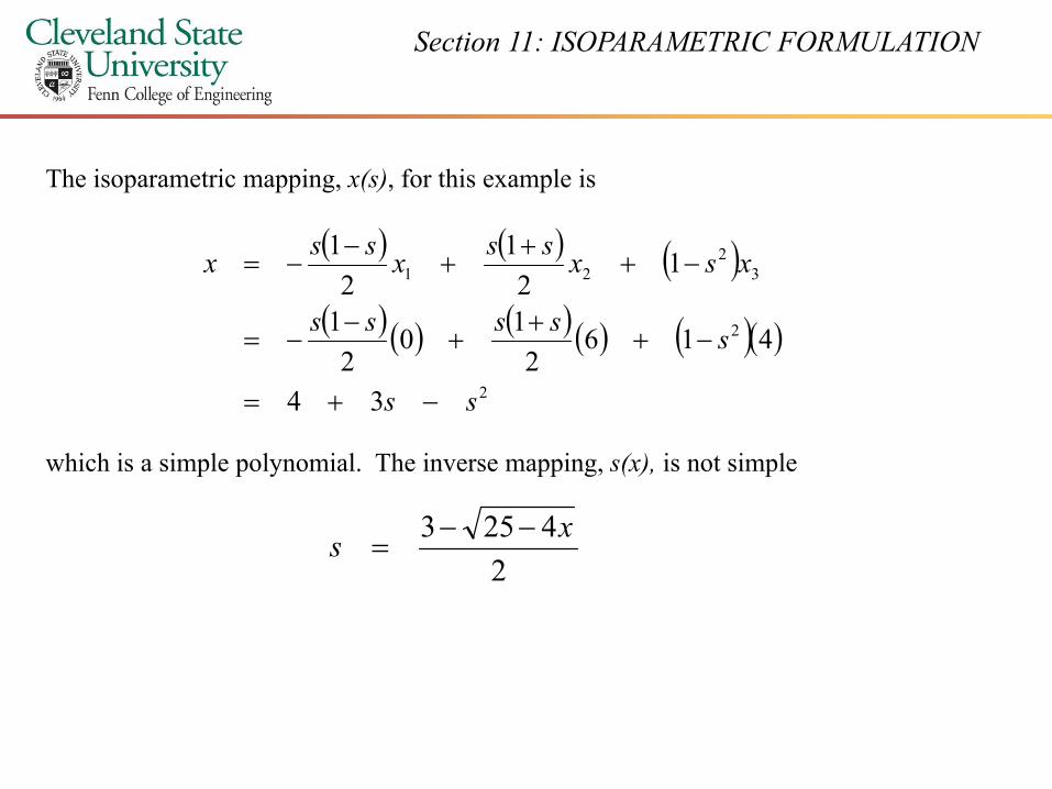
The isoparametric mapping, x(s), for this example is

( ) ( ) ( )( ) ( ) ( ) ( ) ( )( )2

32

21

416101

12

12

1

sssss

xsxssxssx

++

+−

=

−++

+−

−=

( ) ( ) ( ) ( ) ( )( )234

4162

02

ss

s

−+=

−++−=

which is a simple polynomial. The inverse mapping, s(x), is not simple

24253 xs −−

=2


The shape functions in the global coordinates

( )( )

42531

425312

1)(2

xx

sssN

−−

+

−−

+=

( )42521021

21

22

xx −−−=

+

=

Develop expressions for N1 and N3 as a homework exercise.

)(2

2 xN=

p p 1 3


Graphically the shape functions for node #2 plot as follows in the two coordinate systems

N2(x)

1 23

N2(s)

x4 2 11

N2(x)

s1 1 1 23

N2(x) is slightly more complicated N2(s) is a simple polynomial

( )1)( sssN += ( )xxxN 4252101)( −−−=

but is painful to use with more than one element. Think about where to

2)(2 sN = ( )xxxN 425210

2)(2 =

o e e e e t. about w e e toplace the origin of the coordinate system.


Matrices for a Line Element

F li l i h d i h f iFor a line element with quadratic shape functions

{ }{ }dNuNuNuNu ++= 332211

The strain displacement relationship is once again

{ }{ }dN=

xu∂∂

=ε

{ }{ }dB

ux

Nux

Nux

N

=∂∂

+∂∂

+∂∂

= 33

22

11


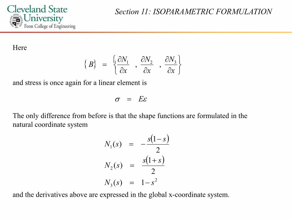
Here

{ }

∂∂∂ NNNB 321

and stress is once again for a linear element is

{ }

∂∂∂=

xxxB 321 ,,

εσ E=

The only difference from before is that the shape functions are formulated in the natural coordinate systemnatural coordinate system

( )

( )1 2

1)( sssN −−=

( )

23

2

1)(2

1)(

ssN

sssN

−=

+=

and the derivatives above are expressed in the global x-coordinate system.


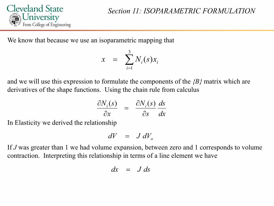
We know that because we use an isoparametric mapping that

∑=3

)( xsNx

and we will use this expression to formulate the components of the {B} matrix which are d i ti f th h f ti U i th h i l f l l

∑=

=1

)(i

ii xsNx

derivatives of the shape functions. Using the chain rule from calculus

dxds

ssN

xsN ii

∂∂

=∂

∂ )()(

In Elasticity we derived the relationship

If J was greater than 1 we had volume expansion between zero and 1 corresponds to volumeodVJdV =

If J was greater than 1 we had volume expansion, between zero and 1 corresponds to volume contraction. Interpreting this relationship in terms of a line element we have

dsJdx =


or

Jdxds 1

=

From a computational standpoint

=dsdxJ

For a line element the calculation immediately above is made, inverted and used in the

∑=

=3

1

)(i

ii x

dssdN

following expression:

=

∂∂

dxds

dssdN

xsN ii )()(

=

∂

dssdN

J

dxdsx

i )(1

Now the derivative of the shape functions are formulated in terms of the natural coordinate system.


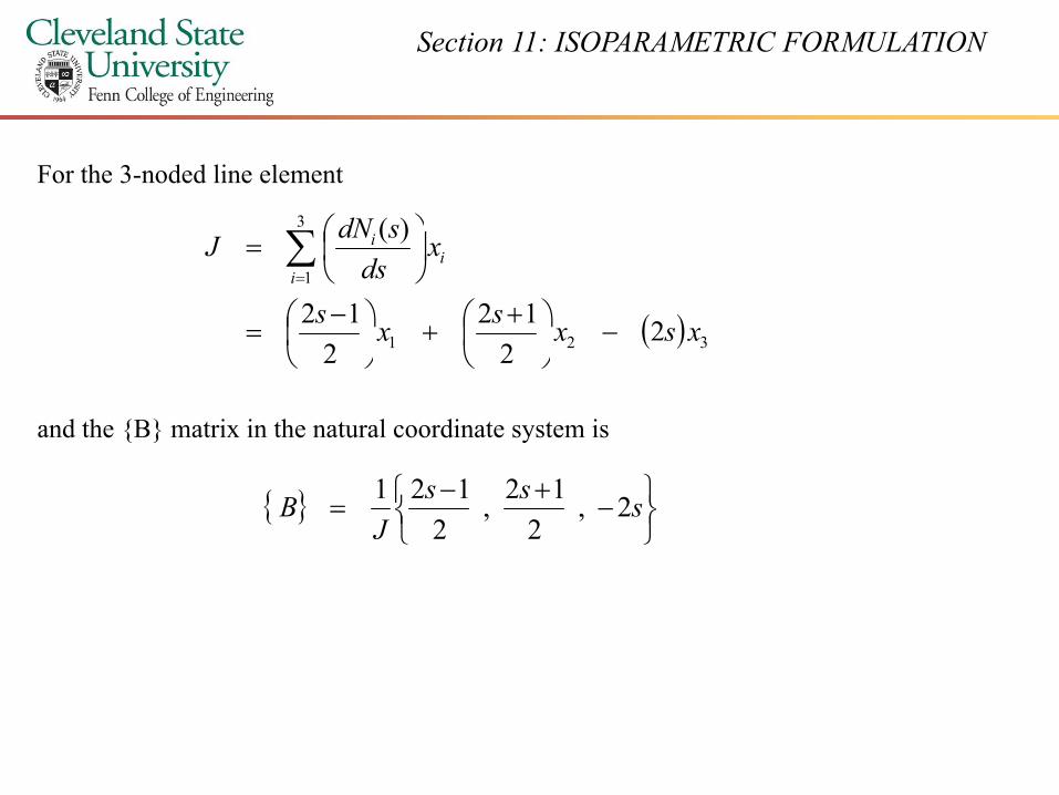
For the 3-noded line element

3 )(sdN

( ) 321

1

21212

)(

xsxsxs

xds

sdNJi

ii

−

+

+

−

=

= ∑

=

and the {B} matrix in the natural coordinate system is

( ) 321 22xsxx

{ }

−

+−= sss

JB 2,

212,

2121


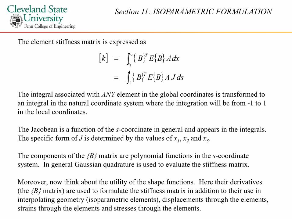
The element stiffness matrix is expressed as

[ ] { } { }∫= 2 dxABEBkx T

The integral associated with ANY element in the global coordinates is transformed to

[ ] { } { }

{ } { }∫

∫

−=

1

1

1

dsJABEB T

x

The integral associated with ANY element in the global coordinates is transformed to an integral in the natural coordinate system where the integration will be from -1 to 1 in the local coordinates.

The Jacobean is a function of the s-coordinate in general and appears in the integrals. The specific form of J is determined by the values of x1, x2 and x3.

The components of the {B} matrix are polynomial functions in the s-coordinateThe components of the {B} matrix are polynomial functions in the s-coordinate system. In general Gaussian quadrature is used to evaluate the stiffness matrix.

Moreover, now think about the utility of the shape functions. Here their derivatives (the {B} matrix) are used to formulate the stiffness matrix in addition to their use in interpolating geometry (isoparametric elements), displacements through the elements, strains through the elements and stresses through the elements.


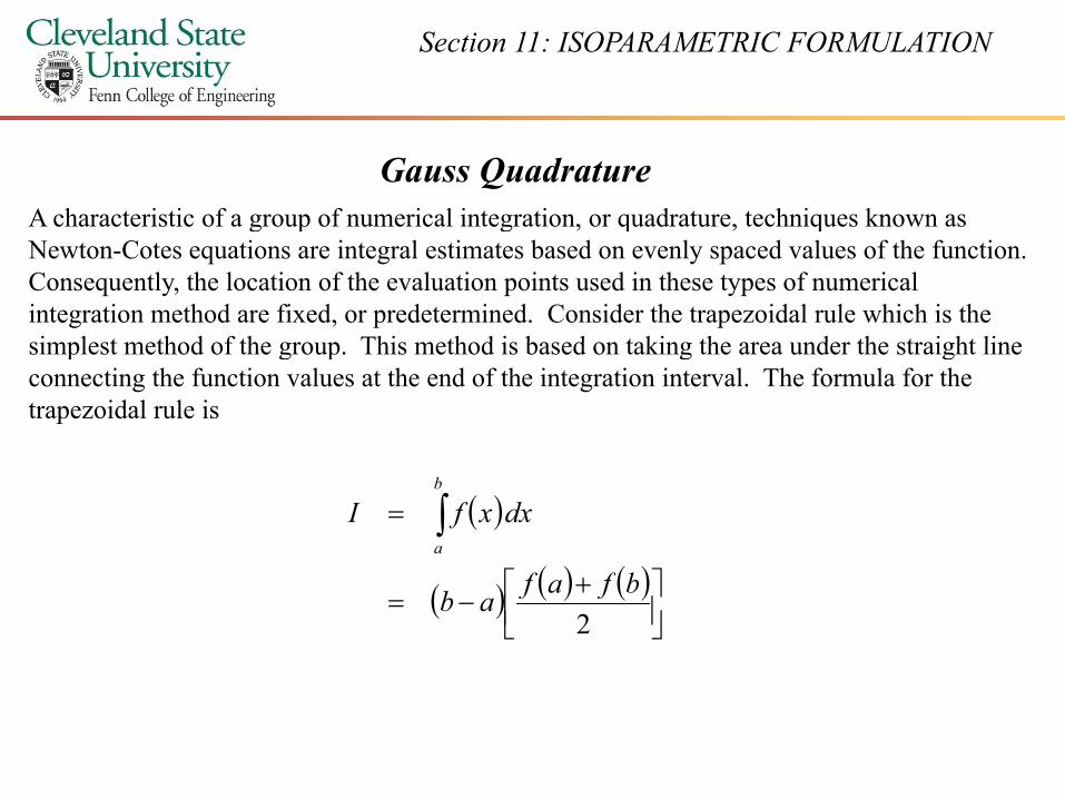
Gauss QuadratureA characteristic of a group of numerical integration, or quadrature, techniques known as g p g , q , qNewton-Cotes equations are integral estimates based on evenly spaced values of the function. Consequently, the location of the evaluation points used in these types of numerical integration method are fixed, or predetermined. Consider the trapezoidal rule which is the simplest method of the gro p This method is based on taking the area nder the straight linesimplest method of the group. This method is based on taking the area under the straight line connecting the function values at the end of the integration interval. The formula for the trapezoidal rule is

( )

( ) ( )

= ∫ dxxfIb

a

( ) ( ) ( )

+

−=2

bfafab


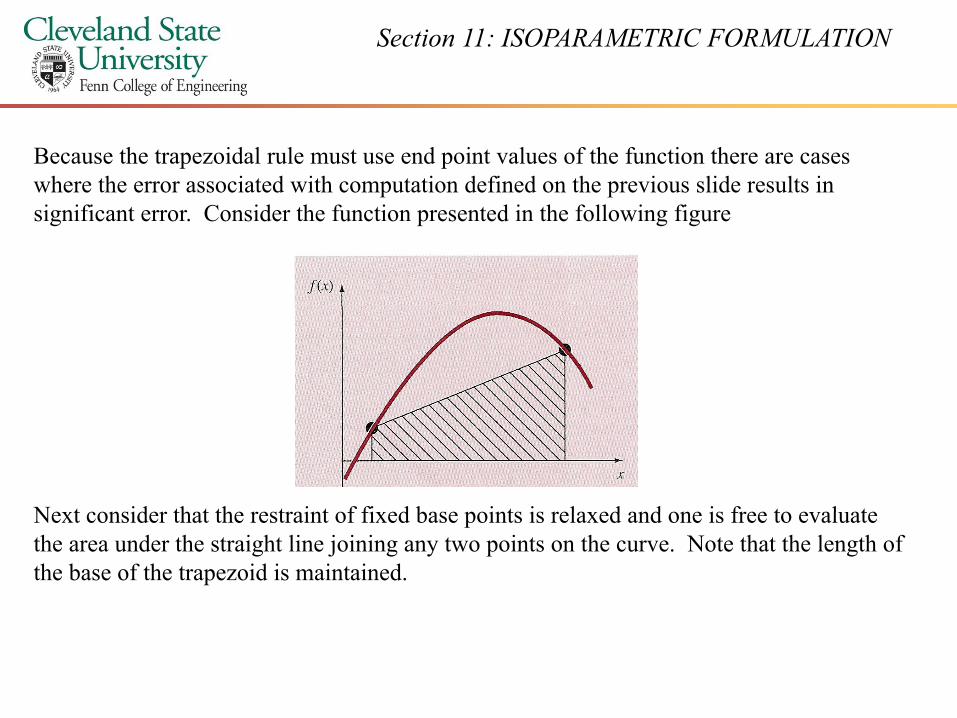
Because the trapezoidal rule must use end point values of the function there are cases where the error associated with computation defined on the previous slide results in i ifi C id h f i d i h f ll i fisignificant error. Consider the function presented in the following figure

Next consider that the restraint of fixed base points is relaxed and one is free to evaluateNext consider that the restraint of fixed base points is relaxed and one is free to evaluate the area under the straight line joining any two points on the curve. Note that the length of the base of the trapezoid is maintained.


By positioning the two points on the curve wisely, a straight line could be positioned that would balance the positive and negative errors. This is depicted in the following figure

Gauss quadrature is the name given to one class of techniques that implement this type of strategy. Before describing the approach and its use in deriving stiffness matrices for isoparametric elements we show how numerical integration formulas such as the trapezoidal rule can be found using the method of undetermined coefficients This methodtrapezoidal rule can be found using the method of undetermined coefficients. This method will then be used to develop the Gauss quadrature formula.


To illustrate the method of undetermined coefficients consider an alternative formulation for the trapezoidal rule bp

( )

( ) ( ) ( )bfafab

dxxfIb

a

+

= ∫

where c and c are constants Realizing the trapezoidal rule must yield exact results when

( ) ( ) ( )

( ) ( )bfcafc

ab

10

2+=

−=

where c0 and c1 are constants. Realizing the trapezoidal rule must yield exact results when the function being integrated is a constant, or a linear function of x, then one can use these results to generate the trapezoidal rule. Consider that for f(x) = 1

( ) ( ) ( )dxcc

ab

ab

=+ ∫−

−−

2

2

10 111

( )ab −=2


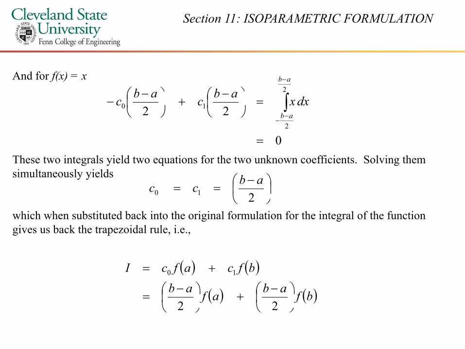
And for f(x) = x2

−

+ −

∫−ab

dabab

0

222

10

=

=

+

− ∫−

−ab

dxxcc

These two integrals yield two equations for the two unknown coefficients. Solving them simultaneously yields

−

==210

abcc

which when substituted back into the original formulation for the integral of the function gives us back the trapezoidal rule, i.e.,

2

( ) ( )

( ) ( )bfabafabbfcafcI

−

+ −

=

+= 10

( ) ( )bfaf

+

22


The objective of the Gauss quadrature approach is to determine the unknown constants for the expression

( ) ( )xfcxfcI +=

However in contrast to the trapezoidal rule that used fixed end points a and b, the function arguments x0 and x1 are not fixed and treated as unknowns. Now we need four integral

i t fi d th f k d

( ) ( )1100 xfcxfcI +=

expressions to find the four unknowns, c0, c1 , x0 and x1.

( ) ( ) ( ) 211

1100 ==+ ∫ dxxfcxfc

We obtain these conditions by assuming the equation above produces the integral value exactly for a constant function and a linear ( ) ( ) ( )

( ) ( ) ( ) 01

11100

11100

==+ ∫

∫

−

−

dxxxfcxfc

ffexactly for a constant function and a linear function. To arrive at two additional conditions the reasoning on the previous overhead is extended and we assume that the

i l fi h i l f b l( ) ( ) ( )

( )32

1

1

1

21100 ==+ ∫

−

dxxxfcxfcequation exactly fits the integral of a parabola (y = x2) and the integral y = x3 exactly. By doing this we determine all four unknowns and in the bargain obtain a two point

( ) ( ) ( ) 01

31100 ==+ ∫

−

dxxxfcxfcg p

integration formula that is exact through cubic polynomials. The four equations are (to the right)


These four equations can be solve simultaneously (homework) for

110 == cc

1

5773503.03

10

10

−=−=x

Thus

5773503.03

11 ==x

11

which yields the interesting result that the simple addition of the function values evaluated at the points above (x x ) yields an integral estimate that is third order accurate

+

−=3

13

1 ffI

the points above (x0, x1) yields an integral estimate that is third order accurate.

Also notice that the integration limits on the previous page were from -1 to +1. This is convenient for isoparametric elements.


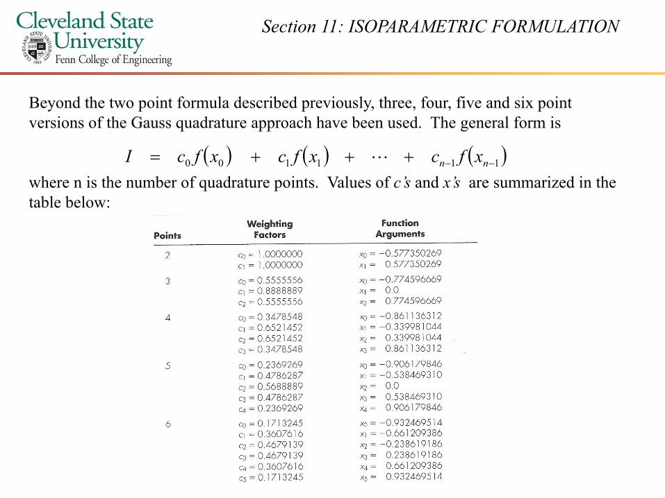
Beyond the two point formula described previously, three, four, five and six point versions of the Gauss quadrature approach have been used. The general form is

where n is the number of quadrature points. Values of c’s and x’s are summarized in the table below:

( ) ( ) ( )111100 −−+++= nn xfcxfcxfcI L


In general for Gauss quadrature we can write

( )∑=n

xfcI

where n is the number of quadrature points for a given variable. If we want to extend this two integration over an area, say for an isoparametric element, then

( )∑=

=i

ii xfcI1

( )

∫

∫ ∫− −

=

n

dtdstsfI

1

1

1

1

1

,

( )

( )∑∑

∫ ∑− =

=

=

nn

iii

tsfcc

dttsfc1 1

,

( )

( )∑∑

∑∑==

=

=

n

ijiij

n

j

ijii

jj

tsfcc

tsfcc

11

11

,

,

In general, we do not have to use the same number of Gauss points in each direction, i.e., idoes not have to equal j, but in finite element analysis this is typically done.

== ij 11


Consider a four point Gauss integration which is shown in following figure

where for an arbitrary function of s and t1 1

( )

( )22

1 1

,

tsfcc

dtdstsfI

nn

=

=

∑∑

∫ ∫==

− −

( )( ) ( ) ( ) ( )2222121221211111

11

,,,,

,

tsfcctsfcctsfcctsfcc

tsfcci

jiijj

+++=

= ∑∑==

where all sampling points are +0.5773 or -0.5773 and all coefficients are equal to one. Hence the double integral is double summation technically, but really it is a single summation over four points in the element, i.e., the Gauss points.


For a volume element we can easily extend the concepts as follows:

∫ ∫ ∫1 1 1

( )

( )∑∑∑

∫ ∫ ∫− − −

=

=

n

kjikji

nn

ztsfccc

dzdtdstsfI1 1 1

,,

,

( )∑∑∑=== k

kjikjiji

ztsfccc111

,,


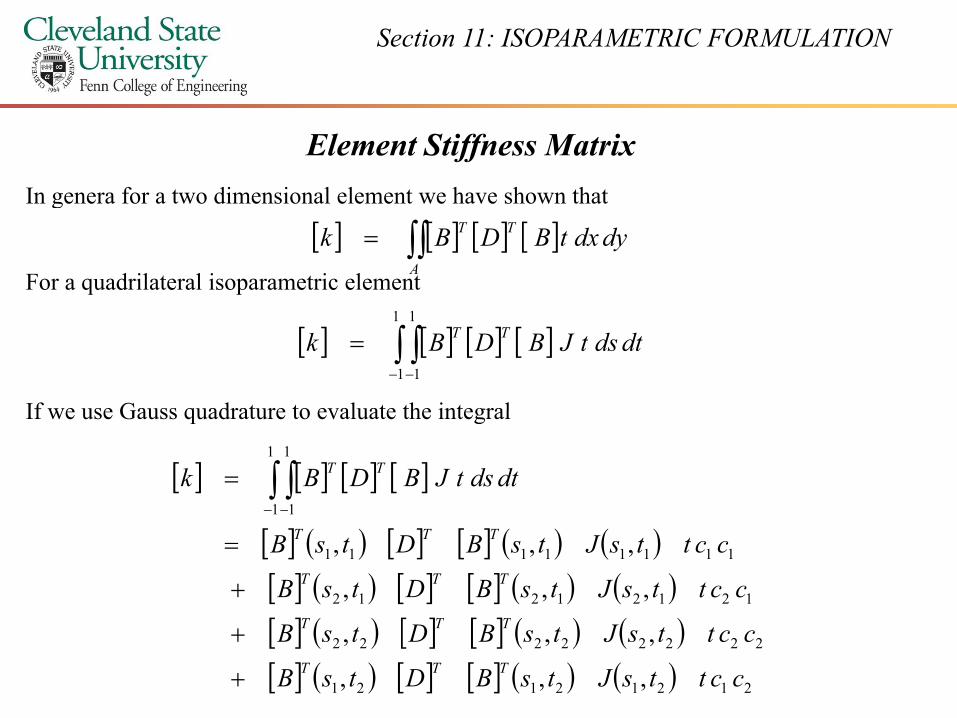
Element Stiffness MatrixIn genera for a two dimensional element we have shown thatg

For a quadrilateral isoparametric element

[ ] [ ] [ ] [ ]∫∫=A

TT dydxtBDBk

If we use Gauss quadrature to evaluate the integral

[ ] [ ] [ ] [ ]∫ ∫− −

=1

1

1

1

dtdstJBDBk TT

If we use Gauss quadrature to evaluate the integral

[ ] [ ] [ ] [ ]1

1

1

1

dtdstJBDBk TT= ∫ ∫− −

[ ] ( ) [ ] [ ] ( ) ( )[ ] ( ) [ ] [ ] ( ) ( ) 12121212

11111111

1 1

,,,

,,,

ccttsJtsBDtsB

ccttsJtsBDtsBTTT

TTT

+

=

[ ] ( ) [ ] [ ] ( ) ( )[ ] ( ) [ ] [ ] ( ) ( ) 21212121

22222222

,,,

,,,

ccttsJtsBDtsB

ccttsJtsBDtsBTTT

TTT

+

+


I Cl E lIn Class Example


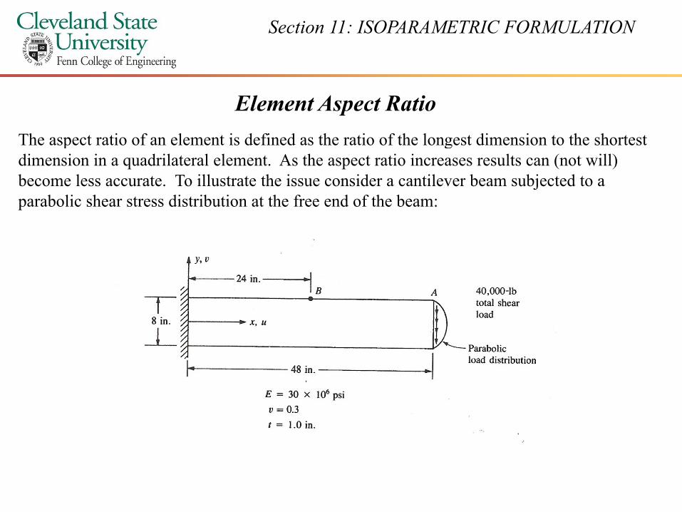
Element Aspect RatioThe aspect ratio of an element is defined as the ratio of the longest dimension to the shortest p gdimension in a quadrilateral element. As the aspect ratio increases results can (not will) become less accurate. To illustrate the issue consider a cantilever beam subjected to a parabolic shear stress distribution at the free end of the beam:


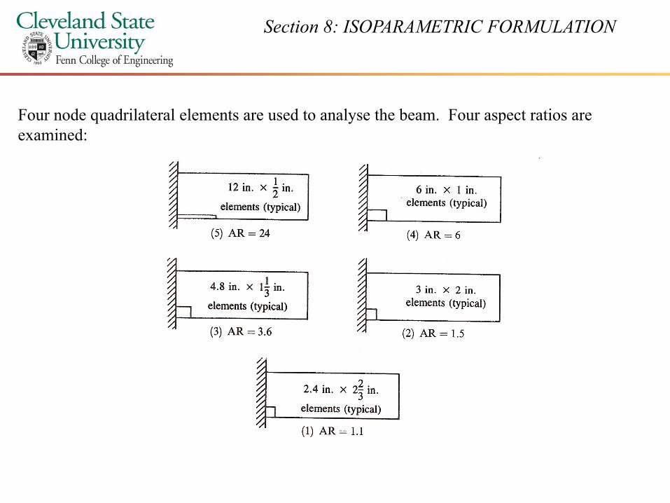
Four node quadrilateral elements are used to analyse the beam. Four aspect ratios are examined:


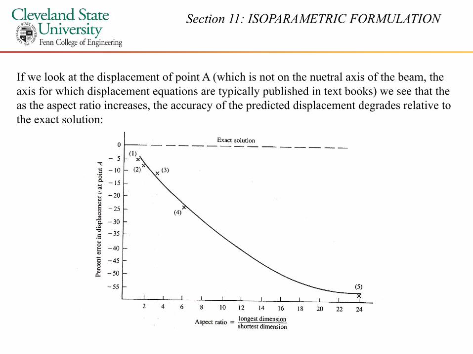
If we look at the displacement of point A (which is not on the nuetral axis of the beam, the axis for which displacement equations are typically published in text books) we see that the

h i i h f h di d di l d d l ias the aspect ratio increases, the accuracy of the predicted displacement degrades relative to the exact solution:


These results are presented in tabular form below:

Note that the previous results were obtained using four node, plane stress quadrilateral elements.


The effects of aspect ratios on the performance of an element is not the same from element to element. The instructor uses higher order brick (volume) elements without any

l f fid li h i d i f i lapparent loss of fidelity when aspect ratios produce warning messages from commercial finite element software.

Still, it is good practice to maintain aspect ratios close to unity. The current generation of fi it l t ft h hi biliti th t ill t ti ll fi t ifinite element software has remeshing capabilities that will automatically fix geometric problems such as the examples shown below:

recap – shape functions - cleveland state universityacademic.csuohio.edu/duffy_s/cve_512_...

Documents