Real-time thermal management of permanent magnetsynchronous motors by resistance estimation

Item type Article

Authors Wilson, S. D.; Stewart, Paul; Stewart, Jill

Citation Real-time thermal management of permanent magnetsynchronous motors by resistance estimation 2012, 6(9):716 IET Electric Power Applications

DOI 10.1049/iet-epa.2010.0232

Publisher IET

Journal IET Electric Power Applications

Rights Archived with thanks to IET Electric Power Applications

Downloaded 27-May-2018 09:02:56

Item License http://creativecommons.org/licenses/by/4.0/

Seediscussions,stats,andauthorprofilesforthispublicationat:https://www.researchgate.net/publication/262600092

Real-timethermalmanagementofpermanentmagnetsynchronousmotorsbyresistanceestimation

ArticleinIETElectricPowerApplications·November2012

DOI:10.1049/iet-epa.2010.0232

READS

68

3authors,including:

PaulStewart

UniversityofDerby

64PUBLICATIONS280CITATIONS

SEEPROFILE

JillStewart

SheffieldHallamUniversity

25PUBLICATIONS76CITATIONS

SEEPROFILE

Allin-textreferencesunderlinedinbluearelinkedtopublicationsonResearchGate,

lettingyouaccessandreadthemimmediately.

Availablefrom:PaulStewart

Retrievedon:09August2016

Published in IET Electric Power ApplicationsReceived on 26th September 2010Revised on 31st October 2011doi: 10.1049/iet-epa.2010.0232

ISSN 1751-8660

Real-time thermal management of permanent magnetsynchronous motors by resistance estimationS.D. Wilson1 P. Stewart2 J. Stewart2

1EA Technology, Capenhurst Technology Park, Capenhurst, Cheshire CH1 6ES, UK2Faculty of Engineering, University of Lincoln, Lincolnshire LN6 7TS, UKE-mail: pstewart@lincoln.ac.uk

Abstract: Real-time thermal management of electrical machines relies on sufficiently accurate indicators of internal temperature.One indicator of temperature in a permanent-magnet synchronous motor is the stator winding resistance. This study applies twocurrent injection techniques to a commercially produced permanent-magnet servomotor, which are applicable under load andcause minimal disturbance to the shaft torque. The current injection techniques applied here enable the temporary boosting ofresistive voltage and consequent application to low-resistance, high-voltage machines. The effectiveness of the approach isdemonstrated by tracking the change in winding temperature during a 2 h load cycle.

1 Introduction

Brushless permanent-magnet machines have emerged as thepreferred electrical machine technology for many applicationsbecause of their high specific power and high efficiency.As is common with other types of electrical machine, theiroutput power is usually limited by the maximum operatingtemperature of key machine components [1]. It is a common,but highly inefficient practice, to design a machine on thebasis of a worst-case estimate of the operating conditions, inorder to protect against over-temperature. A consequence ofthis approach results in the machine operating well below itsmaximum performance for much of its life, particularly inapplications with intermittent or unpredictable duty cycles. Insuch applications, a machine could achieve a transient powerrating that is considerably greater than its continuous rating ifthe thermal capacity of the machine is fully harnessed.

In order to fully exploit the thermal capacity of a machine inapplications with variable and often unpredictable duty cycles,monitoring key temperatures within the machine is vital.Temperature monitoring within a machine could be achievedusing an array of thermal sensors embedded throughout themachine. One drawback of this approach is that therelationship between the sensor and component temperaturesis reliant on the interface properties, particularly in terms ofany time-lags introduced. A ‘sensorless’ approach becomesattractive, whereby estimates of stator coil temperatures canbe obtained by tracking changes in the coil resistance, whichin turn are derived from terminal voltage and currentmeasurements.

Terminal resistance measurements provide a means ofdetermining average coil temperatures, which can be usedas input to a machine-specific thermal model to providemore localised temperature estimates. Winding temperatureestimation also provides information for health monitoring,prognostics and real-time thermal management of a

machine, for example a real-time variable de-rating tomatch the peak transient duty cycle.

In practice, tracking resistance changes in permanent-magnet (PM) machines is extremely challenging,particularly in high-efficiency, high-power machines, wherethe stator resistive voltage drop relative to the net terminalvoltage under normal operating conditions is often verysmall. The experimental machine examined in this paperhas a resistive voltage drop at a rated current of just 1.1%of the terminal voltage, with the parameters of Table 1. Toprovide a temperature resolution as coarse as 108C in thismachine, which represents a realistic objective in order toavoid transient overheating, would require a means ofreliably extracting the true resistive voltage component to aresolution of 0.04%. These difficulties are compounded ina practical drive system by the presence of severaldisturbances in the voltage and current waveforms becauseof a switching ripple; the action of closed-loop controllerswhich continually adjust the current to meet some specifiedcommanded motion; the presence of varying degrees ofmagnetic saturation in the stator, rotor core and rotor saliency.

Notably, resistance estimation methods based on terminalmeasurements cannot usually provide the precision requiredfor high power PM machines. The method described here isbased on intermittent current injection to temporarily boostthe resistive voltage contribution, thus increasing theaccuracy of measurement. Since the thermal time constantof a large PM machine is many orders of magnitude longerthan the duration of the injected pulses, therefore theadditional heating effect within the machine is negligible.

2 Stator-winding resistance estimation

This paper presents a report on the practical implementation(and results) of the ‘Fixed-Magnitude’ method of resistanceestimation, whose theory is presented in [2]. The current

IET Electr. Power Appl., pp. 1–11 1doi: 10.1049/iet-epa.2010.0232 & The Institution of Engineering and Technology 2012

www.ietdl.org

injection and signal separation techniques presented in thispaper are here applied to a drive system controlling acommercially produced interior permanent-magnet (IPM)motor. The current injection techniques enable the temporaryboosting of voltage developed across the winding resistance.Signal separation and resistance estimation algorithms areapplied to determine the resistance parameter. There arevarious reasons why the winding resistance parameter is ofinterest, which are referred to in the Methods paper [2],including the enhancement of motor-control techniques andestimation of the winding temperature. This research isdirected at the latter field, with the estimated resistance beingused to determine the estimated winding temperature.

The stator winding of a typical machine consists of severalinsulated copper coils, whose resistance varies as a functionof coil temperature as

Rs = Rs0 + aRs0(Ts − T0) (1)

where Rs0 is the winding resistance at T08C, Rs is the windingresistance at Ts8C and a is the temperature coefficient ofcopper (3.93 × 1023 per 8C);

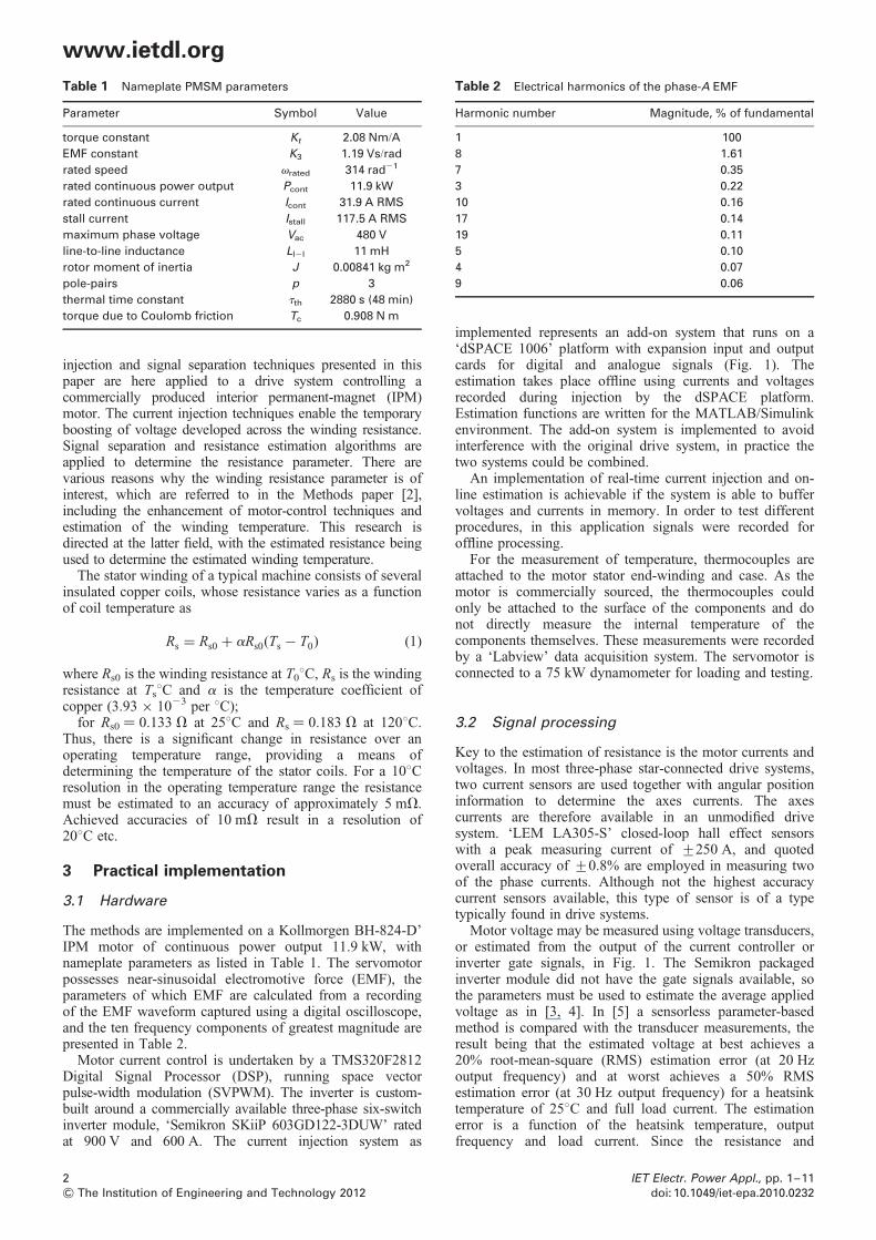
for Rs0 ¼ 0.133 V at 258C and Rs ¼ 0.183 V at 1208C.Thus, there is a significant change in resistance over anoperating temperature range, providing a means ofdetermining the temperature of the stator coils. For a 108Cresolution in the operating temperature range the resistancemust be estimated to an accuracy of approximately 5 mV.Achieved accuracies of 10 mV result in a resolution of208C etc.

3 Practical implementation

3.1 Hardware

The methods are implemented on a Kollmorgen BH-824-D’IPM motor of continuous power output 11.9 kW, withnameplate parameters as listed in Table 1. The servomotorpossesses near-sinusoidal electromotive force (EMF), theparameters of which EMF are calculated from a recordingof the EMF waveform captured using a digital oscilloscope,and the ten frequency components of greatest magnitude arepresented in Table 2.

Motor current control is undertaken by a TMS320F2812Digital Signal Processor (DSP), running space vectorpulse-width modulation (SVPWM). The inverter is custom-built around a commercially available three-phase six-switchinverter module, ‘Semikron SKiiP 603GD122-3DUW’ ratedat 900 V and 600 A. The current injection system as

implemented represents an add-on system that runs on a‘dSPACE 1006’ platform with expansion input and outputcards for digital and analogue signals (Fig. 1). Theestimation takes place offline using currents and voltagesrecorded during injection by the dSPACE platform.Estimation functions are written for the MATLAB/Simulinkenvironment. The add-on system is implemented to avoidinterference with the original drive system, in practice thetwo systems could be combined.

An implementation of real-time current injection and on-line estimation is achievable if the system is able to buffervoltages and currents in memory. In order to test differentprocedures, in this application signals were recorded foroffline processing.

For the measurement of temperature, thermocouples areattached to the motor stator end-winding and case. As themotor is commercially sourced, the thermocouples couldonly be attached to the surface of the components and donot directly measure the internal temperature of thecomponents themselves. These measurements were recordedby a ‘Labview’ data acquisition system. The servomotor isconnected to a 75 kW dynamometer for loading and testing.

3.2 Signal processing

Key to the estimation of resistance is the motor currents andvoltages. In most three-phase star-connected drive systems,two current sensors are used together with angular positioninformation to determine the axes currents. The axescurrents are therefore available in an unmodified drivesystem. ‘LEM LA305-S’ closed-loop hall effect sensorswith a peak measuring current of +250 A, and quotedoverall accuracy of +0.8% are employed in measuring twoof the phase currents. Although not the highest accuracycurrent sensors available, this type of sensor is of a typetypically found in drive systems.

Motor voltage may be measured using voltage transducers,or estimated from the output of the current controller orinverter gate signals, in Fig. 1. The Semikron packagedinverter module did not have the gate signals available, sothe parameters must be used to estimate the average appliedvoltage as in [3, 4]. In [5] a sensorless parameter-basedmethod is compared with the transducer measurements, theresult being that the estimated voltage at best achieves a20% root-mean-square (RMS) estimation error (at 20 Hzoutput frequency) and at worst achieves a 50% RMSestimation error (at 30 Hz output frequency) for a heatsinktemperature of 258C and full load current. The estimationerror is a function of the heatsink temperature, outputfrequency and load current. Since the resistance and

Table 1 Nameplate PMSM parameters

Parameter Symbol Value

torque constant Kt 2.08 Nm/A

EMF constant K3 1.19 Vs/rad

rated speed vrated 314 rad21

rated continuous power output Pcont 11.9 kW

rated continuous current Icont 31.9 A RMS

stall current Istall 117.5 A RMS

maximum phase voltage Vac 480 V

line-to-line inductance Ll2l 11 mH

rotor moment of inertia J 0.00841 kg m2

pole-pairs p 3

thermal time constant tth 2880 s (48 min)

torque due to Coulomb friction Tc 0.908 N m

Table 2 Electrical harmonics of the phase-A EMF

Harmonic number Magnitude, % of fundamental

1 100

8 1.61

7 0.35

3 0.22

10 0.16

17 0.14

19 0.11

5 0.10

4 0.07

9 0.06

2 IET Electr. Power Appl., pp. 1–11

& The Institution of Engineering and Technology 2012 doi: 10.1049/iet-epa.2010.0232

www.ietdl.org

temperature variation thereof induces small changes in thevoltage, the greatest available voltage precision is requiredand the measurements are preferred over the estimates.

‘LEM LV25-P’ voltage transducers are employed to scalethe inverter voltages for input to the dSPACE system.These are closed-loop hall-effect devices with a measuringrange of +400 V, a quoted overall accuracy of +0.8% anda response time of 40 ms. The transducers were mounted inthe motor terminal box. For voltage measurements, acurrent proportional to the measured voltage is passedthrough a high precision resistor in series with the promarycircuit of the transducer. The chosen transducer displayshigh accuracy, linearity, low thermal drift and highbandwidth.

3.3 Implementation

Estimation of the resistance depends on voltage and currentmeasurements. Sampling the current measurements at themidpoint of the SVPWM zero vector resolves thefundamental component of the current waveform, and isripple free. Sampling of the current using this approach isdemonstrated in [6]. The SVPWM voltage waveformconsists of the application of six discrete voltage vectorsper PWM cycle, and contains a high proportion ofharmonics compared with the magnitude of the fundamentalvoltage [7].

The motor control system is augmented with a ‘separate’resistance estimating system, in Fig. 1. It was not possiblefor the dSPACE system to read the sampled voltage andcurrent measurements directly from the DSP, since acompatible communication bus was not available. Bothsystems are therefore required to sample the input signals.Although sampling in the DSP occurs synchronously to the

PWM timers, it does not in the dSPACE system unless adevice provides synchronisation. Use of the synchronisingdevice avoids the problem of the dSPACE system makingconsecutive samples which occur at different times relativeto the start of the PWM cycle.

A stand-alone sample-and-hold board has been designedwhich is triggered by detection of the SVPWM zerovectors. Fig. 2 illustrates the SVPVM vectors that areapplied in a section of the rotor angular position0 , u , 608. The zero vectors are denoted V0 or V7, andeither can be used for sampling. The sensor inputs arelatched while being digitised by the dSPACE system.The sampling instant relative to the zero vector is tunedusing a monostable delay circuit, in Fig. 3. Ideally,sampling should occur at the midpoint of the zero vectorsbut because of a limitation of the practical rig this could notbe achieved. The closest that could be achieved using thesignals available from the DSP was to apply a small timedelay, t1 ¼ 4 ms. The time period t2 was set to 50 ms inorder for the dSPACE system to sample all the inputs in asingle programme cycle time of 67 ms.

All analogue inputs are zero-vector sampled, and anti-aliased with third-order Bessel filters with a cut-offfrequency of 5 kHz, which also facilitate low-pass filteringof the PWM voltages. Analogue Bessel filters were chosensince they are characterised by almost constant group delayacross the entire passband, thus preserving the wave shapeof filtered signals in the passband, allied with ease ofimplementation. The voltages and currents are sampled at16-bit precision, with full-scale deflections set to 400 V and200 A. These were the highest precisions available at15 kHz sampling rate (equal to the SVPWM switchingfrequency), giving at least in principle, voltage and currentresolutions of 12.2 mV and 3 mA.

Fig. 1 Drive system modified to include additional equipment enabling resistance estimation

IET Electr. Power Appl., pp. 1–11 3doi: 10.1049/iet-epa.2010.0232 & The Institution of Engineering and Technology 2012

www.ietdl.org

4 Permanent-magnet synchronous motor(PMSM) dq-axis model

The concept of resolving machine armature quantities intotwo rotating components, one aligned with the field axis,the direct-axis component (d ) and one in quadrature withthe field axis, (q) is a well-established and widely usedmeans of analysing electrical machines. These components,which are stationary with respect to the rotor, are referred toas being in the rotor-stationary frame of reference (qdr).When transferred to the stator-stationary frame of reference,they are referred to as being in the stator-stationary frame ofreference (qds).

The transformation itself can be represented in terms of theelectrical angle between the rotor direct-axis and the statorphase-a axis [8]. Letting S represent the quantity to betransformed (current, voltage or flux), the transformationcan be written in matrix form using Park’s transformation as

Sd

Sq

S0

⎡⎢⎣

⎤⎥⎦= 2

3

cos (u) cos (u− 2p/3) cos (u+ 2p/3)

− sin (u) − sin (u− 2p/3) − sin (u+ 2p/3)

1/2 1/2 1/2

⎡⎢⎣

⎤⎥⎦

×Sa

Sb

Sc

⎡⎢⎣

⎤⎥⎦ (2)

where Sd, Sq and S0 denote the d-axis, q-axis andzero-sequence components of the transformed phasequantities Sa, Sb and Sc.

An equivalent inverse transform exists which transfers thedq0 quantities into stator three-phase quantities. Underbalanced conditions there are no zero-sequence components.When the PMSM three-phase motor equations are alsotransformed into the rotor reference frame the motorvariables may be represented by the following matrix

vdr

vqr

[ ]= Rs −vLq

vLd Rs

[ ]idr

iqr

[ ]+ Ld 0

0 Lq

[ ]d

dt

idr

iqr

[ ]

+ 0Kevm

[ ](3)

where vdr and vqr are the direct and quadrature axes voltages inthe rotor reference frame, idr and iqr are the direct andquadrature axes currents in the rotor reference frame, Rs isthe stator resistance, Ld and Lq are the non-saturated directand quadrature axis inductances, Ke is the back-EMFconstant, v is the electrical frequency and vm is the rotorangular velocity in radians per second.

5 Three-system representation of currentinjection

When the motor is running as part of a drive system, itgenerates a voltage that is defined by the EMF waveform,axes currents and motor parameters such as Ld, and Lq. Thevoltages are described as functions of current by the PMSMvoltage equation denoted G1

vdr

vqr

[ ]=

Rs −vLq(idr, iqr)

vLd(idr, iqr) Rs

[ ]idr

iqr

[ ]

+Ld(idr, iqr) 0

0 Lq(idr, iqr)

[ ]d

dt

idr

iqr

[ ]

+kd(u)vm

kq(u)vm

[ ](4)

where kd, kq are EMF generators and the axes inductances aredescribed as functions of the axes currents. The EMFgenerators represent the variation of the EMF with respectto rotor position and are described in more detail in Section 6.

The voltage of the motor during current injection is the sumof the normal, and ‘injection function’, G2 voltages. Bymanipulation of (4) with d-axis injection current iidr and zeroq-axis injection current, the G2 system equation is formed

vdr = Rsiidr + Ld

d(iidr)

dt(5)

vqr = vLdiidr (6)

The G1 and G2 systems describe the operation of the drivesystem, provided the operation of each system does notaffect the parameters of the other. In practice, when currentis injected (by way of the injection function) it influencesthe parameters describing the G1 and G2 systems throughmagnetic saturation and cross-coupling effects, thus, thefunction, G1, voltage changes. A measurement of the q-axisinductance Lq with respect to d-axis current for thismachine (obtained by sinusoidal excitation on the q-axiswith supply of bias current on the d-axis, in a similarmanner to Stumberger et al. [9]) shows that saturation

Fig. 2 Example per-carrier cycle switching sequence for switchesSa, Sb, Sc, 0 , u , 608, where the zero vectors are hatched anddenoted V0, V7

Fig. 3 Schematic diagram of zero-vector sampling system andrepresentation of delays t1, t2

4 IET Electr. Power Appl., pp. 1–11

& The Institution of Engineering and Technology 2012 doi: 10.1049/iet-epa.2010.0232

www.ietdl.org

accounts for a significant change in the Lq parameter; betweenthe +FA injection current with the bipolar method, and thezero, FA currents of the unipolar method, in Fig. 5. Thevoltage response of this parameter change can berepresented by the use of a third system, G3, whose outputvoltage is a function of the normal operating currents idr, iqr

and the injection current iidr. A representation of theinteraction between the three systems is shown in Fig. 4;where I∗1 and I∗2 are demanded currents for the G1 and G2

systems, respectively, I1, I2 and I3 are current componentsof the G1, G2 and G3 systems, respectively, V1, V2 are thecontroller output voltages, with Vm and Im being themeasured voltages and currents.

The Lq parameter change is responsible for part of thevoltage represented by the G3 system. The system alsogenerates a voltage in response to changes in the Ld, kd andkq parameters. Such changes occur as a result of thedependence of motor parameters on motor currents andspeed. The voltages generated by all three systems sum toproduce the measured voltage Vm. Controller C1 controls themotor function, and C2 controls the current injection function.

Theoretical calculation of the G3 system equations requiresa detailed model, taking into account magnetic saturation, to

be available. Such a model could be produced using materialsdata and finite-element analysis, but is dependent on materialsdata and dimensional information. This information was notavailable for the motor under study. Therefore an empiricalmethod is preferred, whereby resistance estimates areobtained at different operating points (of torque, speed) andcompared with the ‘true’ winding resistance obtained bymeasurement of the winding temperature. The differencebetween the two resistances is assumed to be because of theG3 system, and the approximation of these voltages isdescribed in Section 7.2.

6 EMF waveform

The EMF is the largest component of motor voltage at ratedspeed and torque output. According to the parameters ofTable 1, the EMF comprises 89% of the terminal voltage atrated speed and torque. As described in Part 1, the EMF isseparated from the current injection signals by setting theelectrical angle between injection pulses to Du ¼ npp,where n is an integer number of revolutions. The minimumchoice of n is required to minimise the time betweeninjection pulses, and can be found by analysing the EMFwaveform.

The EMF waveform is recorded at 1000 RPM using adynamometer and digital oscilloscope. The dq-axes EMFsare calculated and presented in Fig. 6, where the q-axisEMF is normalised by subtraction of the mean EMF.

Fig. 6 shows that the EMF varies as a function ofmechanical and electrical positions. The reason for variationwith respect to mechanical position has not beeninvestigated, but is assumed to be because of features ofmanufacturing or electrical abuse of the motor. ThereforeDu ¼ 2pp is required so that successive injection pulsesoccur at identical mechanical positions. The parameters ofthe EMF generator kd(u), that forms part of (4) can befound from the Fourier coefficients of the d-axis EMF,Table 3. Note that these parameters are not required toseparate the motor voltages from the injection voltages, butare presented to illustrate the significant magnitude of theharmonic voltages compared with the resistive voltagemagnitude. That is, the Nd ¼ 1 harmonic generates avoltage which is equivalent to 42% of the injection voltageFRs at F ¼ 50 A and Rs ¼ 0.13 V.

Fig. 5 Measured q-axis inductance as a function of d-axis current

Fig. 4 Motor normal and injection functions with parameterchange compensation

Fig. 6 Normalised dq-Frame EMF

IET Electr. Power Appl., pp. 1–11 5doi: 10.1049/iet-epa.2010.0232 & The Institution of Engineering and Technology 2012

www.ietdl.org

7 Processing system for resistanceestimation

A schematic of the processing functions required to generateresistance estimates is presented in Fig. 7. First, the measuredcurrents and voltages must be converted from functions oftime to functions of position. An interpolation is required toform output data with a constant 360 points per electricalrevolution. This enables the combination of measurementstaken during successive mechanical revolutions, andseparation of the EMF from the injection signal as describedin [2]. Next, the data sets are split into two streams (P1, P2),each stream containing the signals during the application ofeach pulse. These two streams are required to enable thenormal function signals (S(v, i, t)) to be calculated byP1 + P2, and the injection function signals (D(v, i, t)) to becalculated by P1–P2. The D(v, i, t) signals are processed forthe compensation of parameter variation by the G3 compensator.

The current injection methods consist of applying twocurrent pulses. The C2 controller (Fig. 4) applies theunipolar or bipolar method by changing the magnitude ofeach pulse accordingly. The polarities of the bipolar currentinjection pulses are displayed in Fig. 8. The angulardefinition of the pulses is covered in Part 1.

7.1 Post-processing the resistance estimate

Temperature estimation requires a single value to be chosenfor the resistance. The single value is chosen by taking the

mean of Rs over which time the injection current demandmagnitude is equal to F (the window period current is notused for estimation). A small time is allowed to elapse afterthe application of each current pulse while the voltagesettles, and the estimated resistance recorded during thistime is not included.

A single ‘preferred’ value of resistance is thus chosen. Forthe data presented in Fig. 15, this preferred value is 0.127 V.

7.2 G3 system compensation

The G3 system produces a voltage that is dependent on thechange in motor parameters between the first and secondinjection current pulses. For the bipolar method, the d-axiscurrent is defined by the injection current magnitude as+FA. The q-axis current also changes between the pulsesbecause of the influence of the cross-coupling voltages.Both the axes currents influence the axes inductances viamagnetic saturation and therefore provide sample equationsfor the G3 system. For the bipolar method

First pulse:

idr(u1) = −F (7)

iqr(u1) = iqr − Diqr (8)

vdr(u1) = −FRs − vLq( − F)(iqr − Diqr) (9)

Second pulse:

idr(u2) = F (10)

iqr(u2) = iqr + Diqr (11)

vdr(u2) = FRs − vLq(F)(iqr + Diqr) (12)

where iqr is the q-axis mean current over both pulses, and u1,Fig. 7 Schematic of processing functions for resistance estimation

Fig. 8 Bipolar current injection pulses

Table 3 Ten largest Fourier coefficients of d-axis EMF at 1000

RPM

Harmonic number, Nd Magnitude, V/kRPM Angle, 8

1 2.7327 141.0

2 1.5494 1.5

27 0.7795 90.4

0 0.7425 0.0

18 0.4044 289.2

54 0.2525 2105.2

6 0.1108 42.3

4 0.0973 2136.8

26 0.0845 37.4

28 0.0771 237.7

6 IET Electr. Power Appl., pp. 1–11

& The Institution of Engineering and Technology 2012 doi: 10.1049/iet-epa.2010.0232

www.ietdl.org

u2 are ranges of angles for the P1 and P2 pulses. The voltagedifference between the pulses is computed as

Dvdr = vdr(u2) − vdr(u1)

. . . = 2FRs + v(Lq(F) − Lq( − F))iqr (13)

− v(Lq(F) + Lq( − F))Diqr (14)

where the last two terms are proportional to speed. The G3

system voltage is thus proportional to speed. The increasein G3 voltage with speed is demonstrated in Fig. 9, whichcompares the determined injection voltage at 250 RPM withthat at 1250 RPM measured from the experimental rig.

The formula is simplistic in that it defines the G3 voltage asa function of inductance variation because of d-axis saturationonly. In practice, the inductances are functions of both axescurrents in (4), and Diqr is dependent on the currentcontroller’s response to the cross-coupling voltages. Owingto the uncertainty created in the inductance values by thesecurrents, an empirical method is preferred to calculate thevalues of the constants K1, K2 in the following equivalentequation to (14)

Dvdr = 2FRs + vK2iqr + vK1 (15)

To calculate K1 requires K1 and K2 to be set to zero andresistance estimates to be obtained over a speed range.During this test the motor was run with no loading otherthan frictional forces. The end-winding temperature wasrecorded and used to calculate the end-winding resistance.This is assumed to be the value of the winding resistance,and the innovation (difference) between this value and theestimated resistance is displayed in Fig. 10 (Table 4).

The innovation increases with speed, approximated linearlyby the fit line Fit 1, giving K1 ¼ 4 × 1025. Note that thelinear fit for K1 has least error around the 250 RPM mark.

To calculate K2, resistance estimates are obtained with thespeed fixed at 1000 RPM, with K1 ¼ 4 × 1025 and K2 ¼ 0.Resistance estimates are obtained over a range of loadtorques, and the innovation against q-axis current iscalculated and displayed in Fig. 11. The value of K2 isfound from the linear fit line as 4 × 1023. The K1 and K2

values could be determined as functions of speed andcurrent, potentially reducing the error in linearly

approximating the values. The process of determining thecoefficients is schematically presented in Fig. 12. However,in applying this method, care must be taken that theinnovation at every operating point is accurately computed.More accurate computation could potentially be providedby recording temperatures from a network of thermocouplesembedded in the stator winding instead of the single-end-winding thermocouple.

8 Experimental results

The presented results are obtained using the practical setup asdescribed in Section 3. To gauge the performance of theestimation scheme, the different configurations of currentinjection are tested under various loads and speeds. The

Fig. 9 Effect of the G3 signal on the estimated resistance waveform

Table 4 Symbol table

Symbol Parameter

D change in a parameter

u electrical rotor position

uF angle of injected current vector (elec)

v electrical frequency

vm mechanical (shaft) frequency

idr d-axis current, rotor reference frame

iqr q-axis current, rotor reference frame

I1 G1 system current

I2 G2 system current

I3 G3 system current

Im measured current

kd EMF constant for d-axis

kq EMF constant for q-axis

Ld D-axis inductance

Lq Q-axis inductance

Nd D-axis EMF harmonic number

Rs stator resistance

Sa switching signal for inverter phase-A

Sb switching signal for inverter phase-B

Sc switching signal for inverter phase-C

t1 zero-vector sampling delay 1

t2 zero-vector sampling delay 2

vdr d-axis voltage, rotor reference frame

vqr q-axis voltage, rotor reference frame

V0 2 V7 SVPWM vectors

Vm measured voltage

Fig. 10 Determination of the K1 value

IET Electr. Power Appl., pp. 1–11 7doi: 10.1049/iet-epa.2010.0232 & The Institution of Engineering and Technology 2012

www.ietdl.org

current injection pulse train consists of sets of currentinjection pulses with centre angles uc ¼ [0, 120, 240]8.A single estimate is formed from each set of pulses, with50 sets being used to calculate the mean and standarddeviation of the estimates at each operating point. Thefrequency of resistance estimates was set at one estimate(injection of one set of pulses) per second.

8.1 Current pulses and speed disturbance

A single set of current pulses is displayed for the bipolarmethod, in Fig. 13. The six-pulse idr injection current isclearly defined, and the corresponding iqr current displayed.Although q-axis current is not demanded by currentinjection, transiently 40% of the idr current magnitude isgenerated because of imperfect current decoupling.As the idr current flows through the motor, it generates across-coupling voltage on the q-axis. The response of thecurrent controller and inverter to this voltage defines the q-axis current, which is the cause of a small amount of speeddeviation, in Fig. 14.

8.2 Resistance estimates

The resistance estimate for the current pulses displayed inFig. 13 is shown in Fig. 15, where the estimates with centre

angles [0, 120, 240]8 are labelled 1, 2 and 3. A smallnumber of samples elapse after each pulse’s initialapplication during which the resistance is over-estimated(samples 0–50 for Estimate 1). The estimate periodicallybecomes negative, a result of the slightly varying axes

Fig. 13 idr current pulses and coupled iqr current, bipolar method

Fig. 14 Effect of iqr disturbance on speed

Fig. 15 Resistance estimate comprising three applications ofbipolar method at 1000 RPM

Fig. 12 Process to determine K2 and K2 coefficients

Fig. 11 Determination of the K2 value

8 IET Electr. Power Appl., pp. 1–11

& The Institution of Engineering and Technology 2012 doi: 10.1049/iet-epa.2010.0232

www.ietdl.org

currents during injection. The estimated resistance alsobecomes unreliable immediately after the end of the currentpulse (samples .500 for Estimate 1). These periods areignored when calculating the mean estimated resistance,which is 0.129 V for this set of pulses.

Fifty resistance estimates consisting of the bipolar methodapplied for a period of 5408 were taken to demonstrateconvergence to a mean value (Fig. 16). The standarddeviation of the estimates is 3.6 mV, and three standarddeviations are within 8% of the mean value. The nominallysimilar estimates labelled A, B are shown in more detail inFig. 17. The estimates have similar periodic features butdiffer in their mean values by 15 mV.

The difference in the mean values cannot be caused bywinding resistance changes, since the temperature changesslowly. It is proposed that a mechanism exists wherebyparameter change between the two estimates is responsiblefor an error in determining the injection signals D(v, i, t).One mechanism that causes speed and current change is theactions of current and speed controllers on their respectivemeasurements.

The motor current and voltage must be controlled in orderto satisfy demanded torque output and speed. Owing to theinaccuracies of sensors, existence of time-lags andmathematical approximations required to fit a currentcontroller to a drive system, current control will beimperfect. The exhibited features are speed, torque and

voltage deviations which change machine parameters sothat the hypothesis of null change between, and within,periods of current injection is loosely applicable.Improvements in current control have the potential toreduce current ripple and parameter change, in generalrequiring modification to the current control [10–12].

8.3 Evaluation of methods

The bipolar and unipolar methods are compared by applyingeach method at 1000 RPM and without dynamometerloading. The methods are applied with increasing currentmagnitude, from 10 to 60 A. Fifty resistance estimates ateach magnitude of injection current are processed tocalculate the mean and standard deviation of the estimatedresistances, in Fig. 18. The mean resistance is representedby the solid line, the upper and lower bars represent thevalue of resistance one standard deviation above and belowthe mean, respectively.

For each method the mean value changes as the injectioncurrent magnitude is increased, whereas the standarddeviation reduces. The reduction in deviation is due to theincrease in resistive voltage magnitude FRs compared withthe sources of error outlined in the previous section.Therefore the standard deviation reduces, and the resistanceestimates become increasingly accurate as the injectioncurrent magnitude F increases to a point, in Fig. 18.

For a given current magnitude F, the standard deviation ofthe unipolar method is approximately twice that of the bipolarmethod. The increased confidence in the value of theresistance is due to the generation of twice the resistivevoltage (after the P1–P2 operation) per ampere of injectioncurrent magnitude.

8.4 Resistance estimation accuracy across a speedrange

The accuracy of resistance estimation across a speed range isassessed by taking 50 estimates at each 125 RPM speed step,from 250 to 2000 RPM. The temperature of the end windingwas recorded over the length of the test in order to provide athermally derived estimate of winding resistance againstwhich the resistance estimation scheme is compared, inFig. 19. The mean of the estimated resistance remainswithin 10% (258C) of the winding resistance until

Fig. 16 Convergence of estimates: A ¼ max, B ¼ min

Fig. 17 Comparison of estimates A and B

Fig. 18 Dependence of the mean and standard deviation of theestimates on the injection current magnitude

IET Electr. Power Appl., pp. 1–11 9doi: 10.1049/iet-epa.2010.0232 & The Institution of Engineering and Technology 2012

www.ietdl.org

1250 RPM. Note that the winding resistance is inferred fromthermocouple temperature measurement at the surface of theend-winding, which was the only accessible part of thewinding bundle. Inferring the winding resistance in thismanner cannot account for the end-winding temperaturebeing different from the average temperature of the wholewinding. The winding resistance should not be consideredaccurate. However, the trend of a slowly changingtemperature is considered common to the end-winding andthe winding as a whole by virtue of their connection.

Above 1500 RPM the estimate becomes inaccurate becauseof the error in linearly approximating the G3 system voltage,whose magnitude increases substantially above 1500 RPM, inFig. 10. With the practical setup as described this limited thespeed range for resistance estimation to vmax/2. The speedrange could in theory be extended by representing K1 as afunction of speed rather than a linear approximation asdisplayed in Fig. 10, but care must be taken in obtainingaccurate estimates of the winding resistance.

8.5 Accuracy across a torque range

Fifty estimates are taken at each torque setting, with motorq-axis currents in the range 225 to 30 A (278 to 94%Icont). The estimates are processed to determine the meanand standard deviation of the estimated resistances, inFig. 20. The mean of the estimates shows deviation up to

+5.7% of the average resistance value, equating to anuncertainty in temperature of +148C. The variation invalue is due to the different machine inductances atdifference levels of q-axis current. Hence, the accuracy ofresistance estimation is again dependent on the G3 systemcompensation. The accuracy across the torque range couldin theory be improved by storing K2 as a function of q-axiscurrent rather than a linear approximation as displayed inFig. 11. In this case, due care must be taken in establishingprecise winding resistance.

8.6 Temperature estimation

The motor was thermally cycled by dynamometer control ofthe load torque. Over a 2 h period, the motor was loaded to50 A q-axis current (150% rated, origin �A) for 30 min,65 A (200% rated) until the end-winding measured 908(A � B) and the temperature stabilised at 85% for 30 minby loading to �40 A (125% rated, B � C). The load wasthen reduced to zero and the motor cooling assisted with afan until the remaining time elapsed. The end-windingtemperature is displayed in Fig. 21a. During this period,motor load was temporarily reduced to zero every 40 s topermit current injection. Note that it is not prudent toinduce large magnitude d-axis currents under high torqueoutput because of the risk of demagnetisation. Theestimates are processed off-line by a 17-point moving

Fig. 19 Effect of machine speed on estimated resistance

Fig. 20 Effect of load torque on estimation accuracy

Fig. 21 Estimated resistance and measured temperature over 2 hload cycle

a Temperature estimatesb Resistance estimates

10 IET Electr. Power Appl., pp. 1–11

& The Institution of Engineering and Technology 2012 doi: 10.1049/iet-epa.2010.0232

www.ietdl.org

average filter ‘MA(17)’ and recursive least-squares filter withforgetting factor 1/13, ‘RLS(13)’. These processing methodsare compared in Fig. 21b. Note that these filters suffer fromend-effects at the start and end of the x-axis.

RLS(13) lags MA(17), and is prone to oscillation in theB � C region. Increasing the forgetting factor removes theoscillations, but at the cost of a greater time lag. Betweenthe origin and point ‘A’ the initial high rate of windingtemperature increase is mirrored in the resistance increases,followed by a period of lower-rate heating. Between points‘A’ and ‘B’ the winding temperature rises quickly as theload is increased. The filtered estimates also rise at high rates.

Between points ‘B’ and ‘C’ the winding temperatureremains constant at 858. MA(17) best approximates theconstant temperature, whereas the RLS(13) filter is prone todeviations. From point ‘C’ the exponential cooling is bestdetected by MA(17), with less time-lag than RLS(13).

The resistance estimated from the moving average filter isconverted to an equivalent temperature using the windingresistance of 0.129 V at 258C, and presented with themeasured end-winding temperature for comparativepurposes, in Fig. 21a. Note that the end-windings composeonly a section of the winding, are not in contact with theback-iron and attain a different temperature to that of thewinding as a whole.

9 Conclusion

An evaluation of the fixed-magnitude resistance-estimatingmethods proposed in [2] is presented. Similar to othersignal injection methods, the motor load current andresistance sense currents are decoupled. Since the motordoes not have to be loaded to enable resistance estimation,it may take place on-demand. The new methods, unlikeother signal injection-based methods; do not require themotor star point to be available, and there is no directgeneration of pulsating torque. Hence, there is greater scopefor application.

These features are avoided in the new technique byseparating the sense current and voltage from the loadcurrent and voltage; not by provision of a different circuitfor the sense current, nor by provision of a frequencydifference between the sense and load currents. Instead, theseparation is achieved by hypothesising that change in themotor parameters is negligibly small between onerevolution and the next. The sensing signals are computedin the current and voltage differences between revolutionswith, and without sense current; or between revolutionswith opposite polarities of sense currents. Digitallycontrolled, inverter-driven drive systems require augmentingwith the necessary voltage measuring equipment, estimationfunctions and additional inverter VA (if estimation isdesired during high-load periods) to enable the benefits ofresistance and temperature estimation.

A chief advantage of the method is the elimination of theuse of parameters in describing motor voltages. As theparameters are not estimated, the computationalrequirements can be reduced. The only parameters explicitlyrequired are two experimentally determined values K1, K2,although the simple tuning process outlined in this paperrequires further work to improve and identify itsapplicability to different machines.

The methods have been tested on a commercially producedservomotor that exhibits significant change in the inductanceparameter with current magnitude. The load current flowing

through the machine resistance at full load develops avoltage less than 1.1% of the EMF at rated speed. Thisfeature creates difficult conditions for resistance estimatingmethods.

In practice, the estimated resistance is sensitive to speedand torque variations, which is reflected in the estimationsfor the machine described in this paper. Uncertainty in thetrue value of the resistance is reduced by using multipleapplications of the method, which are then processed by amoving-average filter. The filtered estimates are accurateenough to be used for temperature estimation, demonstratedthrough a thermal cycle of the test motor. In certain areas ofthe machine torque and speed envelope, it is not possible toinject the required sense current, because of the availableinverter voltage or consideration of de-magnetisationeffects. However, at least some of these regions areeminently suitable for complementary methods based onload-current sensing. In conjunction with such methods, theoverall solution is able to provide the on-demand resistanceestimation that enables the real-time thermal management ofPMSMs.

10 Acknowledgment

S.D. Wilson was supported by a grant from the Engineeringand Physical Sciences Research Council (EPSRC) and aCo-operative Award in Science and Engineering (CASE)provided by Rolls-Royce PLC. Technical support, and thehardware used in this research were provided by theEPSRC Project Zero-Constraint Free Piston EnergyConverter, Grant Number: GR/S97507/01.

11 References

1 Bonnet, A.H.: ‘Root cause ac motor failure analysis’, IEEE Trans. Ind.Appl., 2000, 36, (5), pp. 1435–1448

2 Taylor, B., Wilson, S., Stewart, P.: ‘Methods of resistance estimation inpermanent magnet synchronous motors for real-time thermalmanagement’, IEEE Trans. Energy Convers., 2010, 25, pp. 698–707

3 Kim, H.-W., Youn, M., Cho, K., Kim, H.-S.: ‘Nonlinearity estimationand compensation of pwm vsi for pmsm under resistance and fluxlinkage uncertainty’, IEEE Trans. Control Syst. Technol., 2006, 14,(4), pp. 589–601

4 Guerrero, J., Leetma, M., Briz, F., Zamorron, A., Lozenz, R.: ‘Inverternonlinearity effects in high-frequency signal-injection-based sensorlesscontrol methods’, IEEE Trans. Ind. Appl., 2005, 41, (2), pp. 618–626

5 Yu, X., Dunnigan, M., Williams, B.: ‘Phase voltage estimation of a pwmvsi and its application to vector-controlled induction machine parameterestimation’, IEEE Trans. Ind. Electron., 2000, 47, (5), pp. 1181–1185

6 Blasko, V., Kaura, V., Niewiadomski, W.: ‘Sampling of discontinuousvoltage and current signals in electrical drives: a system approach’,IEEE Trans. Ind. Appl., 1998, 34, (5), pp. 1123–1130

7 Holmes, D., Lipo, T.: ‘Pulse-width modulation for power converters’(IEEE Press, 2003)

8 Fitzgerald, A., Charles Kingsley, J., Umans, S.D.: ‘Electric machinery’(McGraw-Hill, 2003)

9 Stumberger, B., Stumberger, G., Dolinar, D., Hamler, A., Trlep, M.:‘Evaluation of saturation and cross-magnetization effects in interiorpermanent-magnet synchronous motor’, IEEE Trans. Ind. Appl., 2003,39, (5), pp. 1264–1271

10 Angelo, C.D., Bossio, G., Solsona, J., Garcia, G., Valla, M.:‘Mechanical sensorless speed control of permanent-magnet ac motorsdriving an unknown load’, IEEE Trans. Ind. Electron., 2006, 53, (2),pp. 406–414

11 Grcar, B., Cafuta, P., Stumberger, G., Stankovic, A.: ‘Control-basedreduction of pulsating torque for pmac machines’, IEEE Trans.Energy Convers., 2002, 17, (2), pp. 169–175

12 Ferretti, G., Magnani, G., Rocco, P.: ‘Modeling, identification, andcompensation of pulsating torque in permanent magnet ac motors’,IEEE Trans. Ind. Electron., 1998, 45, (6), pp. 912–920

IET Electr. Power Appl., pp. 1–11 11doi: 10.1049/iet-epa.2010.0232 & The Institution of Engineering and Technology 2012

www.ietdl.org