permanent magnet brushless dc

8/8/2019 Permanent Magnet Brushless DC

http://slidepdf.com/reader/full/permanent-magnet-brushless-dc 1/31

Massachusetts Institute of TechnologyDepartment of Electrical Engineering and Computer Science

6.685 Electric Machines

Class Notes 7: Permanent Magnet “Brushless DC” Motors September 5, 2005c�2005 James L. Kirtley Jr.

1 Introduction

This document is a brief introduction to the design evaluation of permanent magnet motors, withan eye toward servo and drive applications. It is organized in the following manner: First, wedescribe three different geometrical arrangements for permanent magnet motors:

1. Surface Mounted Magnets, Conventional Stator,

2. Surface Mounted Magnets, Air-Gap Stator Winding, and

3. Internal Magnets (Flux Concentrating).

After a qualitative discussion of these geometries, we will discuss the elementary rating parameters of the machine and show how to arrive at a rating and how to estimate the torque and powervs. speed capability of the motor. Then we will discuss how the machine geometry can be used toestimate both the elementary rating parameters and the parameters used to make more detailedestimates of the machine performance.

Some of the more involved mathematical derivations are contained in appendices to this note.

2 Motor Morphologies

There are, of course, many ways of building permanent magnet motors, but we will consider only a

few in this note. Actually, once these are understood, rating evaluations of most other geometricalarrangements should be fairly straightforward. It should be understood that the “rotor inside” vs.“rotor outside” distinction is in fact trivial, with very few exceptions, which we will note.

2.1 Surface Magnet Machines

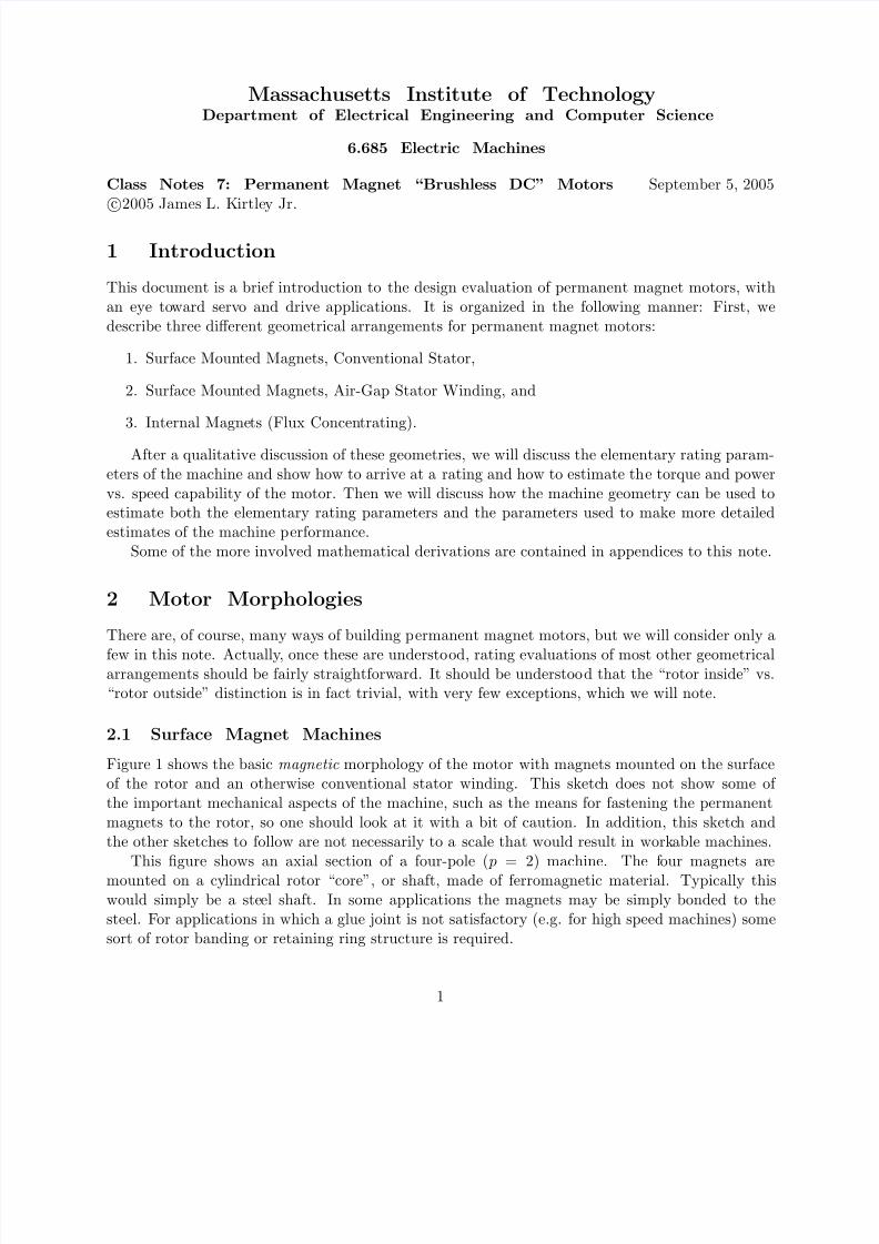
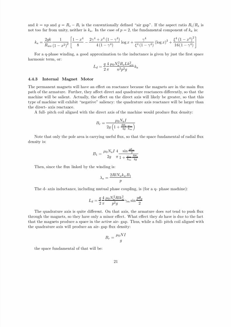
Figure 1 shows the basic magnetic morphology of the motor with magnets mounted on the surfaceof the rotor and an otherwise conventional stator winding. This sketch does not show some of the important mechanical aspects of the machine, such as the means for fastening the permanentmagnets to the rotor, so one should look at it with a bit of caution. In addition, this sketch andthe other sketches to follow are not necessarily to a scale that would result in workable machines.

This gure shows an axial section of a four-pole ( p = 2) machine. The four magnets aremounted on a cylindrical rotor “core”, or shaft, made of ferromagnetic material. Typically thiswould simply be a steel shaft. In some applications the magnets may be simply bonded to thesteel. For applications in which a glue joint is not satisfactory (e.g. for high speed machines) somesort of rotor banding or retaining ring structure is required.

1



Rotor Core(Shaft)Stator Winding

in Slots

RotorMagnets

Stator Core

Air−Gap

Figure 1: Axial View of a Surface Mount Motor

The stator winding of this machine is “conventional”, very much like that of an induction motor,consisting of wires located in slots in the surface of the stator core. The stator core itself is made of laminated ferromagnetic material (probably silicon iron sheets), the character and thickness of thesheets determined by operating frequency and efficiency requirements. They are required to carryalternating magnetic elds, so must be laminated to reduce eddy current losses.

This sort of machine is simple in construction. Note that the operating magnetic ux density inthe air-gap is nearly the same as in the magnets, so that this sort of machine cannot have air-gapux densities higher than that of the remanent ux density of the magnets. If low cost ferritemagnets are used, this means relatively low induction and consequently relatively low efficiencyand power density. (Note the qualier “relatively” here!). Note, however, that with modern, highperformance permanent magnet materials in which remanent ux densities can be on the order of 1.2 T, air-gap working ux densities can be on the order of 1 T. With the requirement for slots tocarry the armature current, this may be a practical limit for air-gap ux density anyway.

It is also important to note that the magnets in this design are really in the “air gap” of the machine, and therefore are exposed to all of the time- and space- harmonics of the statorwinding MMF. Because some permanent magnets have electrical conductivity (particularly thehigher performance magnets), any asynchronous elds will tend to produce eddy currents andconsequent losses in the magnets.

2.2 Interior Magnet or Flux Concentrating Machines

Interior magnet designs have been developed to counter several apparent or real shortcomings of surface mount motors:

• Flux concentrating designs allow the ux density in the air-gap to be higher than the uxdensity in the magnets themselves.

2



• In interior magnet designs there is some degree of shielding of the magnets from high orderspace harmonic elds by the pole pieces.

• There are control advantages to some types of interior magnet motors, as we will show anon.Essentially, they have relatively large negative saliency which enhances “ux weakening” forhigh speed operation, in rather direct analogy to what is done in DC machines.

• Some types of internal magnet designs have (or claim) structural advantages over surfacemount magnet designs.

Slots

StatorCore

Rotor PolePieces

Armature in

RotorMagnets

Non−magneticRotor Core(shaft)

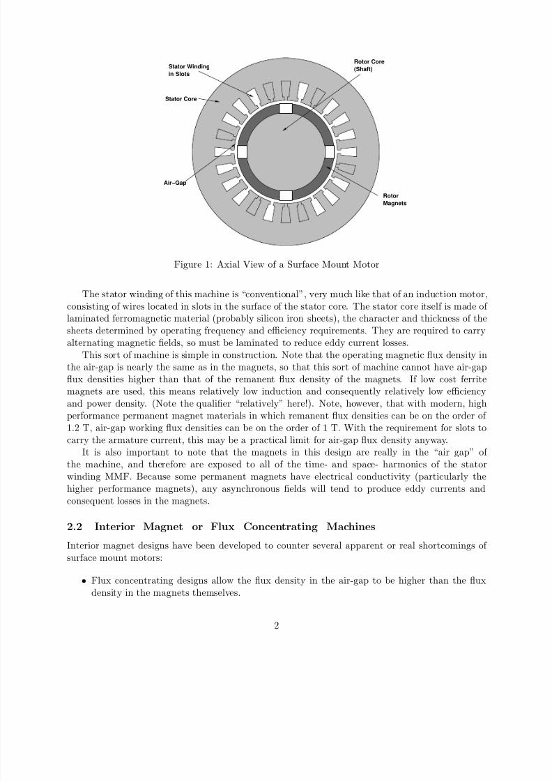
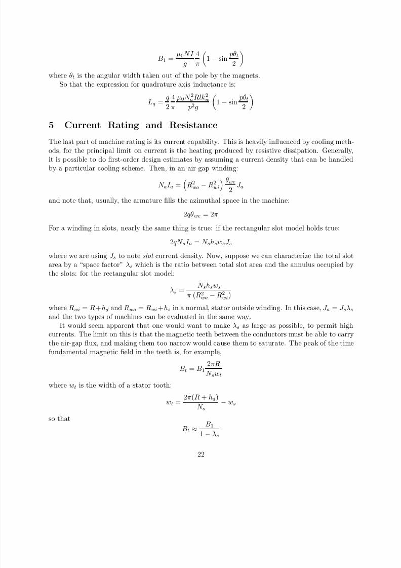
Figure 2: Axial View of a Flux Concentrating Motor

The geometry of one type of internal magnet motor is shown (crudely) in Figure 2. Thepermanent magnets are oriented so that their magnetization is azimuthal. They are located betweenwedges of magnetic material (the pole pieces) in the rotor. Flux passes through these wedges,going radially at the air- gap, then azimuthally through the magnets. The central core of the rotormust be non-magnetic, to prevent “shorting out” the magnets. No structure is shown at all inthis drawing, but quite obviously this sort of rotor is a structural challenge. Shown is a six-polemachine. Typically, one does not expect ux concentrating machines to have small pole numbers,because it is difficult to get more area inside the rotor than around the periphery. On the otherhand, a machine built in this way but without substantial ux concentration will still have saliencyand magnet shielding properties.

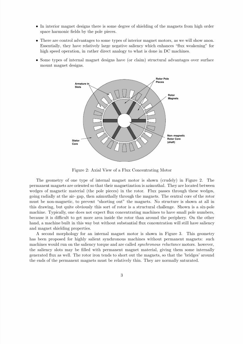
A second morphology for an internal magnet motor is shown in Figure 3. This geometry

has been proposed for highly salient synchronous machines without permanent magnets: suchmachines would run on the saliency torque and are called synchronous reluctance motors. however,the saliency slots may be lled with permanent magnet material, giving them some internallygenerated ux as well. The rotor iron tends to short out the magnets, so that the ’bridges’ aroundthe ends of the permanent magnets must be relatively thin. They are normally saturated.

3



Stator Core

Stator Slots

Air Gap

Rotor

Saliency Slots

Figure 3: Axial View of Internal Magnet Motor

At rst sight, these machines appear to be quite complicated to analyze, and that judgementseems to hold up.

2.3 Air Gap Armature Windings

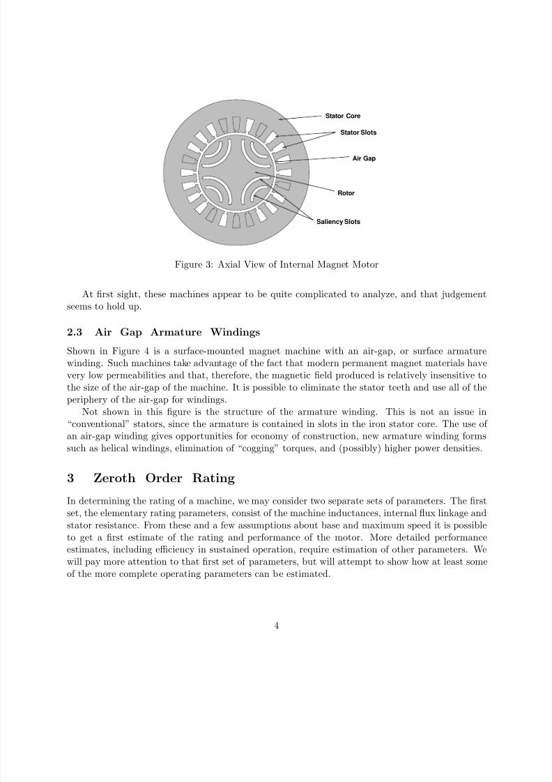
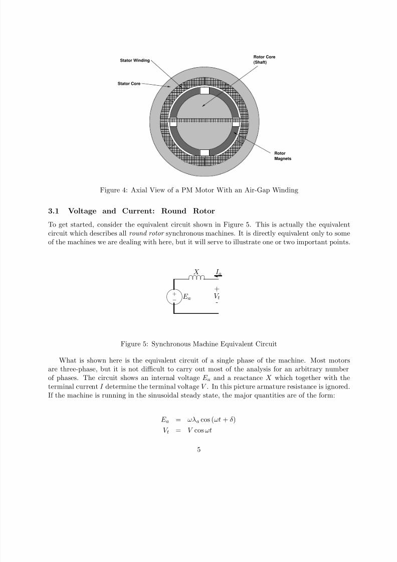
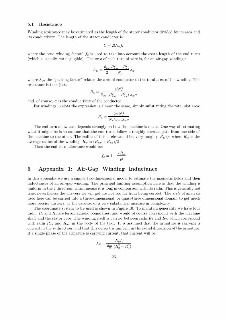
Shown in Figure 4 is a surface-mounted magnet machine with an air-gap, or surface armaturewinding. Such machines take advantage of the fact that modern permanent magnet materials havevery low permeabilities and that, therefore, the magnetic eld produced is relatively insensitive tothe size of the air-gap of the machine. It is possible to eliminate the stator teeth and use all of theperiphery of the air-gap for windings.

Not shown in this gure is the structure of the armature winding. This is not an issue in“conventional” stators, since the armature is contained in slots in the iron stator core. The use of an air-gap winding gives opportunities for economy of construction, new armature winding formssuch as helical windings, elimination of “cogging” torques, and (possibly) higher power densities.

3 Zeroth Order Rating

In determining the rating of a machine, we may consider two separate sets of parameters. The rstset, the elementary rating parameters, consist of the machine inductances, internal ux linkage andstator resistance. From these and a few assumptions about base and maximum speed it is possibleto get a rst estimate of the rating and performance of the motor. More detailed performanceestimates, including efficiency in sustained operation, require estimation of other parameters. Wewill pay more attention to that rst set of parameters, but will attempt to show how at least someof the more complete operating parameters can be estimated.

4



-�

+

Rotor CoreStator Winding (Shaft)

Stator Core

0 0 0 0 0 0 0 0 0 0 0 0 0 0 00 0 0 0 0 0 0 0 0 0 0 0 0 0 00 0 0 0 0 0 0 0 0 0 0 0 0 0 00 0 0 0 0 0 0 0 0 0 0 0 0 0 00 0 0 0 0 0 0 0 0 0 0 0 0 0 00 0 0 0 0 0 0 0 0 0 0 0 0 0 00 0 0 0 0 0 0 0 0 0 0 0 0 0 00 0 0 0 0 0 0 0 0 0 0 0 0 0 00 0 0 0 0 0 0 0 0 0 0 0 0 0 00 0 0 0 0 0 0 0 0 0 0 0 0 0 00 0 0 0 0 0 0 0 0 0 0 0 0 0 00 0 0 0 0 0 0 0 0 0 0 0 0 0 00 0 0 0 0 0 0 0 0 0 0 0 0 0 00 0 0 0 0 0 0 0 0 0 0 0 0 0 00 0 0 0 0 0 0 0 0 0 0 0 0 0 00 0 0 0 0 0 0 0 0 0 0 0 0 0 00 0 0 0 0 0 0 0 0 0 0 0 0 0 00 0 0 0 0 0 0 0 0 0 0 0 0 0 00 0 0 0 0 0 0 0 0 0 0 0 0 0 00 0 0 0 0 0 0 0 0 0 0 0 0 0 0

1 1 1 1 1 1 1 1 1 1 1 1 1 1 1 11 1 1 1 1 1 1 1 1 1 1 1 1 1 1 11 1 1 1 1 1 1 1 1 1 1 1 1 1 1 11 1 1 1 1 1 1 1 1 1 1 1 1 1 1 11 1 1 1 1 1 1 1 1 1 1 1 1 1 1 11 1 1 1 1 1 1 1 1 1 1 1 1 1 1 11 1 1 1 1 1 1 1 1 1 1 1 1 1 1 11 1 1 1 1 1 1 1 1 1 1 1 1 1 1 11 1 1 1 1 1 1 1 1 1 1 1 1 1 1 11 1 1 1 1 1 1 1 1 1 1 1 1 1 1 11 1 1 1 1 1 1 1 1 1 1 1 1 1 1 11 1 1 1 1 1 1 1 1 1 1 1 1 1 1 11 1 1 1 1 1 1 1 1 1 1 1 1 1 1 11 1 1 1 1 1 1 1 1 1 1 1 1 1 1 11 1 1 1 1 1 1 1 1 1 1 1 1 1 1 11 1 1 1 1 1 1 1 1 1 1 1 1 1 1 11 1 1 1 1 1 1 1 1 1 1 1 1 1 1 11 1 1 1 1 1 1 1 1 1 1 1 1 1 1 11 1 1 1 1 1 1 1 1 1 1 1 1 1 1 11 1 1 1 1 1 1 1 1 1 1 1 1 1 1 1

0 0 0 0 0 0 0 0 0 0 0 0 0 0 01 1 1 1 1 1 1 1 1 1 1 1 1 1 1 1

RotorMagnets0 0 0 0 0 0 0 0 0 0 0 0 0 0 00 0 0 0 0 0 0 0 0 0 0 0 0 0 00 0 0 0 0 0 0 0 0 0 0 0 0 0 01 1 1 1 1 1 1 1 1 1 1 1 1 1 1 11 1 1 1 1 1 1 1 1 1 1 1 1 1 1 11 1 1 1 1 1 1 1 1 1 1 1 1 1 1 1

Figure 4: Axial View of a PM Motor With an Air-Gap Winding

3.1 Voltage and Current: Round Rotor

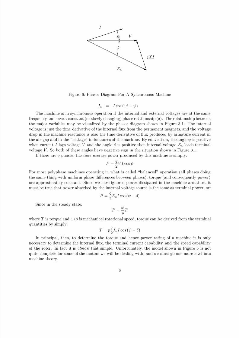
To get started, consider the equivalent circuit shown in Figure 5. This is actually the equivalentcircuit which describes all round rotor synchronous machines. It is directly equivalent only to someof the machines we are dealing with here, but it will serve to illustrate one or two important points.

X I a ∩∩∩∩

+ E a V t −

Figure 5: Synchronous Machine Equivalent Circuit

What is shown here is the equivalent circuit of a single phase of the machine. Most motorsare three-phase, but it is not difficult to carry out most of the analysis for an arbitrary numberof phases. The circuit shows an internal voltage E a and a reactance X which together with theterminal current I determine the terminal voltage V . In this picture armature resistance is ignored.If the machine is running in the sinusoidal steady state, the major quantities are of the form:

E a = ωλ a cos ( ωt + δ)V t = V cos ωt

5



� �

I

� � � � � � � � � � ψ V

δ

jXI

E a

Figure 6: Phasor Diagram For A Synchronous Machine

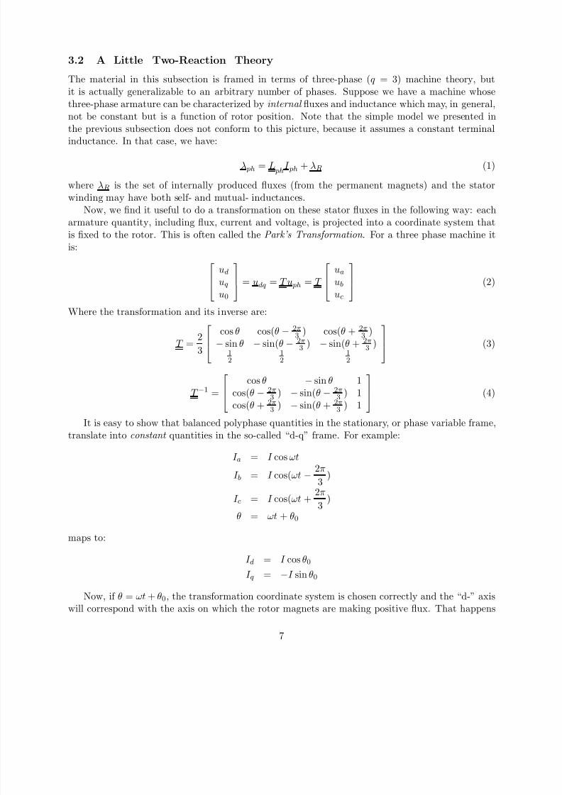
I a = I cos ( ωt − ψ)

The machine is in synchronous operation if the internal and external voltages are at the same

frequency and have a constant (or slowly changing) phase relationship ( δ). The relationship betweenthe major variables may be visualized by the phasor diagram shown in Figure 3.1. The internalvoltage is just the time derivative of the internal ux from the permanent magnets, and the voltagedrop in the machine reactance is also the time derivative of ux produced by armature current inthe air-gap and in the “leakage” inductances of the machine. By convention, the angle ψ is positivewhen current I lags voltage V and the angle δ is positive then internal voltage E a leads terminalvoltage V . So both of these angles have negative sign in the situation shown in Figure 3.1.

If there are q phases, the time average power produced by this machine is simply:

P =q

V I cos ψ 2

For most polyphase machines operating in what is called “balanced” operation (all phases doing

the same thing with uniform phase differences between phases), torque (and consequently power)are approximately constant. Since we have ignored power dissipated in the machine armature, itmust be true that power absorbed by the internal voltage source is the same as terminal power, or:

qP = E a I cos ( ψ − δ)

2Since in the steady state:

ω P = T

p

where T is torque and ω/p is mechanical rotational speed, torque can be derived from the terminalquantities by simply:

qT = p λ a I cos ( ψ − δ)

2In principal, then, to determine the torque and hence power rating of a machine it is only

necessary to determine the internal ux, the terminal current capability, and the speed capabilityof the rotor. In fact it is almost that simple. Unfortunately, the model shown in Figure 5 is notquite complete for some of the motors we will be dealing with, and we must go one more level intomachine theory.

6



3.2 A Little Two-Reaction Theory

The material in this subsection is framed in terms of three-phase ( q = 3) machine theory, butit is actually generalizable to an arbitrary number of phases. Suppose we have a machine whosethree-phase armature can be characterized by internal uxes and inductance which may, in general,not be constant but is a function of rotor position. Note that the simple model we presented inthe previous subsection does not conform to this picture, because it assumes a constant terminalinductance. In that case, we have:

λ ph = L ph I ph + λR (1)

where λR is the set of internally produced uxes (from the permanent magnets) and the statorwinding may have both self- and mutual- inductances.

Now, we nd it useful to do a transformation on these stator uxes in the following way: eacharmature quantity, including ux, current and voltage, is projected into a coordinate system thatis xed to the rotor. This is often called the Park’s Transformation . For a three phase machine itis:

ud ua

uq = udq = T u ph = T ub (2)u0 uc

Where the transformation and its inverse are:

cos θ cos(θ − 23π ) cos( θ + 2

3π ) 2π T =

2 − sin θ − sin(θ − 3 ) − sin(θ + 23π ) (3)

3 1 1 12 2 2

cos θ − sin θ 1 2π 2π T − 1 = cos(θ − 3 ) − sin(θ − 3 ) 1 (4)2πcos(θ + 2

3π ) − sin(θ + 3 ) 1

It is easy to show that balanced polyphase quantities in the stationary, or phase variable frame,translate into constant quantities in the so-called “d-q” frame. For example:

I a = I cos ωt 2π

I b = I cos(ωt − )3

2π I c = I cos(ωt + )

3θ = ωt + θ0

maps to:

I d = I cos θ0

I q = − I sin θ0

Now, if θ = ωt + θ0 , the transformation coordinate system is chosen correctly and the “d-” axiswill correspond with the axis on which the rotor magnets are making positive ux. That happens

7



if, when θ = 0, phase A is linking maximum positive ux from the permanent magnets. If this isthe case, the internal uxes are:

λ aa = λ f cos θ 2π

λ ab = λ f cos(θ − )3

2π λ ac = λ f cos(θ + )3

Now, if we compute the uxes in the d-q frame, we have:

λdq = L dq I dq + λR = T L T − 1I dq + λR (5) ph

Now: two things should be noted here. The rst is that, if the coordinate system has been chosenas described above, the ux induced by the rotor is, in the d-q frame, simply:

λ f

λR = 0 (6)

0

That is, the magnets produce ux only on the d- axis.The second thing to note is that, under certain assumptions, the inductances in the d-q frame

are independent of rotor position and have no mutual terms. That is:

Ld 0 0

L = T L T − 1 = 0 Lq 0 (7)dq ph 0 0 L0

The assertion that inductances in the d-q frame are constant is actually questionable, but it isclose enough to being true and analyses that use it have proven to be close enough to being correctthat it (the assertion) has held up to the test of time. In fact the deviations from independenceon rotor position are small. Independence of axes (that is, absence of mutual inductances in thed-q frame) is correct because the two axes are physically orthogonal. We tend to ignore the third,or “zero” axis in this analysis. It doesn’t couple to anything else and has neither ux nor currentanyway. Note that the direct- and quadrature- axis inductances are in principle straightforward tocompute. They are

direct axis the inductance of one of the armature phases (corrected for the fact of multiple phases)with the rotor aligned with the axis of the phase, and

quadrature axis the inductance of one of the phases with the rotor aligned 90 electrical degreesaway from the axis of that phase.

Next, armature voltage is, ignoring resistance, given by:d d

V ph =dt

λ ph = T − 1λdq (8)dt

and that the transformed armature voltage must be:

8



V dq = T V ph

d = T (T − 1λdq )

dt d d

= λdq + ( T T − 1)λdq (9)dt dt

The second term in this expresses “speed voltage”. A good deal of straightforward but tediousmanipulation yields:

0 − dθ 0dt d dθ T T − 1 = dt 0 0 (10)

dt 0 0 0The direct- and quadrature- axis voltage expressions are then:

dλdV d = − ωλq (11)dt

dλqV q = + ωλd (12)dt

wheredθ

ω =dt

Instantaneous power is given by:

P = V a I a + V bI b + V cI c (13)

Using the transformations given above, this can be shown to be:3 3

P =2

V dI d +2

V q I q + 3 V 0I 0 (14)

which, in turn, is:

P = ω 3

2(λdI q − λq I d) +

3

2(dλd

dt I d +

dλq

dt I q ) + 3

dλ 0

dt I 0 (15)

Then, noting that ω = pΩ and that (15) describes electrical terminal power as the sum of shaftpower and rate of change of stored energy, we may deduce that torque is given by:

qT = p(λdI q − λq I d) (16)

2Note that we have stated a generalization to a q- phase machine even though the derivation

given here was carried out for the q = 3 case. Of course three phase machines are by far themost common case. Machines with higher numbers of phases behave in the same way (and thisgeneralization is valid for all purposes to which we put it), but there are more rotor variablesanalogous to “zero axis”.

Now, noting that, in general, Ld and Lq are not necessarily equal,

λd = LdI d + λ f (17)λq = Lq I q (18)

then torque is given by:q

T = p (λ f + ( Ld − Lq ) I d ) I q (19)2

9



3.3 Finding Torque Capability

For high performance drives, we will generally assume that the power supply, generally an inverter,can supply currents in the correct spatial relationship to the rotor to produce torque in somereasonably effective fashion. We will show in this section how to determine, given a required torque(or if the torque is limited by either voltage or current which we will discuss anon), what thevalues of I d and I q must be. Then the power supply, given some means of determining where therotor is (the instantaneous value of θ), will use the inverse Park’s transformation to determine theinstantaneous valued required for phase currents. This is the essence of what is known as “eldoriented control”, or putting stator currents in the correct location in space to produce the requiredtorque.

Our objective in this section is, given the elementary parameters of the motor, nd the capabilityof the motor to produce torque. There are three things to consider here:

• Armature current is limited, generally by heating,

• A second limit is the voltage capability of the supply, particularly at high speed, and

• If the machine is operating within these two limits, we should consider the optimal placement

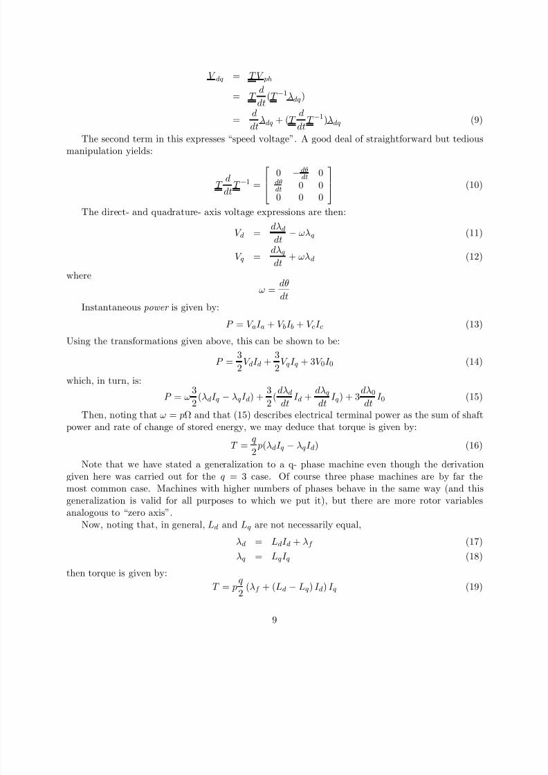
of currents (that is, how to get the most torque per unit of current to minimize losses).Often the discussion of current placement is carried out using, as a tool to visualize what is

going on, the I d , I q plane. Operation in the steady state implies a single point on this plane.A simple illustration is shown in Figure 7. The thermally limited armature current capability isrepresented as a circle around the origin, since the magnitude of armature current is just the lengthof a vector from the origin in this space. In general, for permanent magnet machines with buriedmagnets, Ld < L q , so the optimal operation of the machine will be with negative I d . We will showhow to determine this optimum operation anon, but it will in general follow a curve in the I d , I q

plane as shown.Finally, an ellipse describes the voltage limit. To start, consider what would happen if the

terminals of the machine were to be short-circuited so that V = 0. If the machine is operating at

sufficiently high speed so that armature resistance is negligible, armature current would be simply:λ f I d = −Ld

I q = 0

Now, loci of constant ux turn out to be ellipses around this point on the plane. Since terminalux is proportional to voltage and inversely proportional to frequency, if the machine is operatingwith a given terminal voltage, the ability of that voltage to command current in the I d , I q plane isan ellipse whose size “shrinks” as speed increases.

To simplify the mathematics involved in this estimation, we normalize reactances, uxes, currents and torques. First, let us dene the base ux to be simply λb = λ f and the base current I b to

be the armature capability. Then we dene two per-unit reactances:Ld I b

xd = (20)λb

Lq I b xq = (21)

λb

10



For sufficiently low speeds, the power electronic drive can command the optimal current toproduce torque up to rated. However, for speeds higher than the “Base Speed”, this is no longertrue. Dene a per-unit terminal ux:

V ψ =

ωλb

Operation at a given ux magnitude implies:

ψ2 = (1 + xd id )2 + ( xq iq )2

which is an ellipse in the id , iq plane. The Base Speed is that speed at which this ellipse crosses thepoint where the optimal current curve crosses the armature capability. Operation at the highestattainable torque (for a given speed) generally implies d-axis currents that are higher than thoseon the optimal current locus. What is happening here is the (negative) d-axis current serves toreduce effective machine ux and hence voltage which is limiting q-axis current. Thus operationabove the base speed is often referred to as “ux weakening”.

The strategy for picking the correct trajectory for current in the id , iq plane depends on thevalue of the per-unit reactance xd . For values of xd > 1, it is possible to produce some torque at any speed. For values of xd < 1, there is a speed for which no point in the armature current capability is

within the voltage limiting ellipse, so that useful torque has gone to zero. Generally, the maximumtorque operating point is the intersection of the armature current limit and the voltage limitingellipse:

2 2q − ψ2 + 1 xxd xdid = (26)− +2

d 2d

2d 2

q 2q − x 2

q − x− xx x x

2diq = 1 − i (27)

It may be that there is no intersection between the armature capability and the voltage limitingellipse. If this is the case and if xd < 1, torque capability at the given speed is zero.

If, on the other hand, xd > 1, it may be that the intersection between the voltage limitingellipse and the armature current limit is not the maximum torque point. To nd out, we calculatethe maximum torque point on the voltage limiting ellipse. This is done in the usual way bydifferentiating torque with respect to id while holding the relationship between id and iq to be onthe ellipse. The algebra is a bit messy, and results in:

22d

2d xd ) (ψ2 − 1) +3xd (xq − xd ) −3xd (xq − xd) − (xq −xx xdid = − (28)− +2 (xqd − 2 (xqd − 2

d4x xd) 4x xd) 2 ( xq − xd) x1

iq = ψ2 − (1 + xd id )2 (29)xq

Ordinarily, it is probably easiest to compute (28) and (29) rst, then test to see if the currentsare outside the armature capability, and if they are, use (26) and (27).

These expressions give us the capability to estimate the torque-speed curve for a machine. Asan example, the machine described by the parameters cited in Table 1 is a (nominal) 3 HP, 4-pole,3000 RPM machine.

The rated operating point turns out to have the following attributes:

12



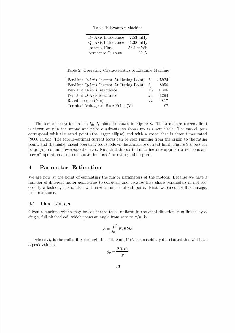
Table 1: Example Machine

D- Axis Inductance 2.53 mHyQ- Axis Inductance 6.38 mHyInternal Flux 58.1 mWbArmature Current 30 A

Table 2: Operating Characteristics of Example Machine

Per-Unit D-Axis Current At Rating Point id -.5924Per-Unit Q-Axis Current At Rating Point iq .8056Per-Unit D-Axis Reactance xd 1.306Per-Unit Q-Axis Reactance xq 3.294Rated Torque (Nm) T r 9.17Terminal Voltage at Base Point (V) 97

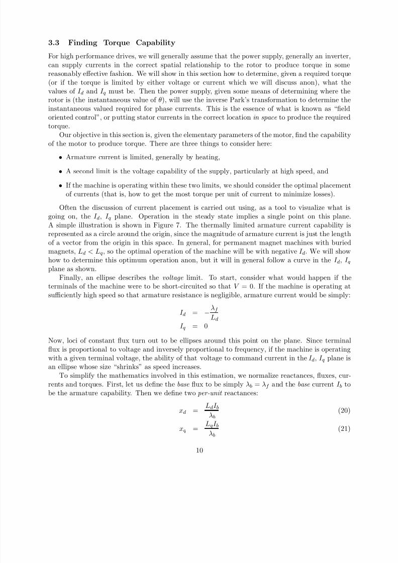
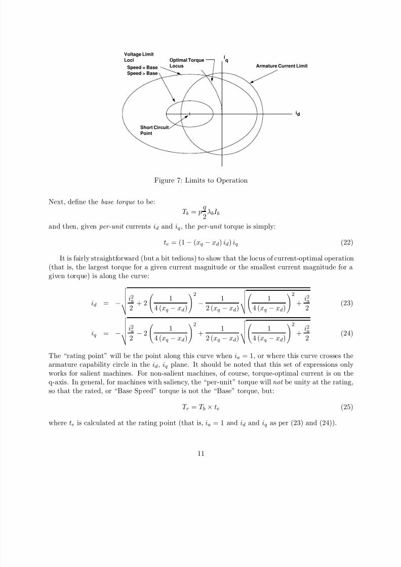
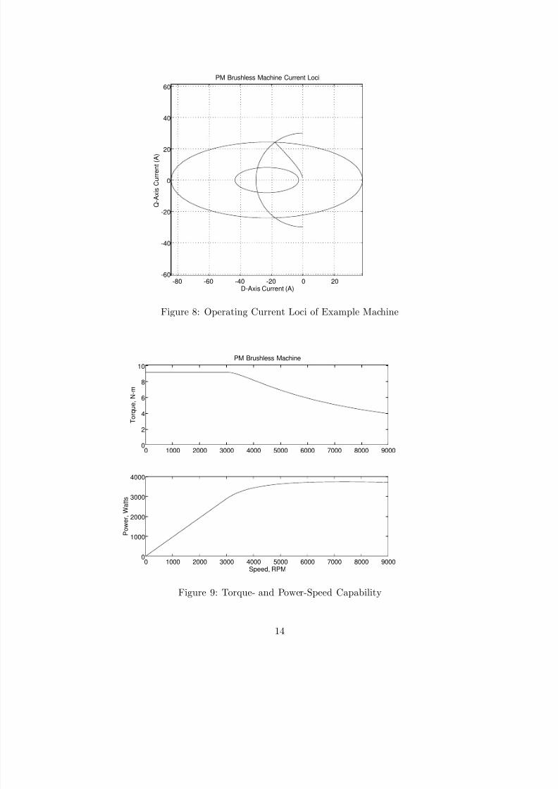
The loci of operation in the I d , I q plane is shown in Figure 8. The armature current limitis shown only in the second and third quadrants, so shows up as a semicircle. The two ellipsescorrespond with the rated point (the larger ellipse) and with a speed that is three times rated(9000 RPM). The torque-optimal current locus can be seen running from the origin to the ratingpoint, and the higher speed operating locus follows the armature current limit. Figure 9 shows thetorque/speed and power/speed curves. Note that this sort of machine only approximates “constantpower” operation at speeds above the “base” or rating point speed.

4 Parameter Estimation

We are now at the point of estimating the major parameters of the motors. Because we have anumber of different motor geometries to consider, and because they share parameters in not tooorderly a fashion, this section will have a number of sub-parts. First, we calculate ux linkage,then reactance.

4.1 Flux Linkage

Given a machine which may be considered to be uniform in the axial direction, ux linked by asingle, full-pitched coil which spans an angle from zero to π/p , is:

φ = B r Rldφ 0

where B r is the radial ux through the coil. And, if B r is sinusoidally distributed this will havea peak value of

2RlB rφ p = p

13

πp



0

PM Brushless Machine Current Loci60

40

20

0

-20

-40

-60

Q - A x i s

C u r r e n t ( A

)

-80 -60 -40 -20 0 20D-Axis Current (A)

Figure 8: Operating Current Loci of Example Machine

PM Brushless Machine

0

2

4

6

8

10

T o r q u e ,

N - m

1000 2000 3000 4000 5000 6000 7000 8000 9000

0

1000

2000

3000

4000

P o w e r ,

W a t t s

1000 2000 3000 4000 5000 6000 7000 8000 9000Speed, RPM

Figure 9: Torque- and Power-Speed Capability

14

0



Now, if the actual winding has N a turns, and using the pitch and breadth factors derived inAppendix 1, the total ux linked is simply:

2RlB 1N a kwλ f = (30) p

where

kw = k pkb α

k p = sin2

sin m γ

kb = 2m sin γ

2

The angle α is the pitch angle,N pα = 2 πp N s

where N p is the coil span (in slots) and N s is the total number of slots in the stator. The angle γ is the slot electrical angle:

2πp

γ = N s

Now, what remains to be found is the space fundamental magnetic ux density B1. In Appendix2 it is shown that, for magnets in a surface-mount geometry, the magnetic eld at the surface of the magnetic gap is:

B1 = µ0M 1kg (31)

where the space-fundamental magnetization is:

B r 4 pθmM 1 = sinµ0 π 2

where B r is remanent ux density of the permanent magnets and θm is the magnet angle.and where the factor that describes the geometry of the magnetic gap depends on the case. For

magnets inside and p = 1,

R p− 1 pR p+1 − R p+1 p

R i 2 p 1− p 1− p

2 p 2 1 + R1 − R2skg =

R s − R i 2 p p + 1 p − 1

For magnets inside and p = 1,

1 1kg =

R2 − R2 R22 − R2 + R i

2 logR2

2 1 R1s i

For the case of magnets outside and p = 1:

R i p− 1 p

R p+1 − R p+1 1 − p 1− pkg =R s − R i

2 p p + 1+

pR2 p R1 − R22 p 2 1 p − 1 s

and for magnets outside and p = 1,

15



1 12 − R2 + R2 R2

2 R1kg =

R2 − R2 R21 s log

s i

Where R s and R i are the outer and inner magnetic boundaries, respectively, and R2 and R1are the outer and inner boundaries of the magnets.

Note that for the case of a small gap, in which both the physical gap g and the magnet thicknesshm are both much less than rotor radius, it is straightforward to show that all of the above expressions approach what one would calculate using a simple, one-dimensional model for the permanentmagnet:

hmkg →g + hm

This is the whole story for the winding-in-slot, narrow air-gap, surface magnet machine. For air-gap armature windings, it is necessary to take into account the radial dependence of the magneticeld.

4.2 Air-Gap Armature WindingsWith no windings in slots, the conventional denition of winding factor becomes difficult to apply.If, however, each of the phase belts of the winding occupies an angular extent θw , then the equivalentto (31) is:

sin p θw

kw = θw

2

p 2

Next, assume that the “density” of conductors within each of the phase belts of the armaturewinding is uniform, so that the density of turns as a function of radius is:

2N a r N (r ) =

R2 − R2wo wi

This just expresses the fact that there is more azimuthal room at larger radii, so with uniformdensity the number of turns as a function of radius is linearly dependent on radius. Here, Rwo andRwi are the outer and inner radii, respectively, of the winding.

Now it is possible to compute the ux linked due to a magnetic eld distribution:

R wo 2lN a kw r 2r λ f =

R2 − R2 µ0H r (r )dr (32) pR wi wo wi

Note the form of the magnetic eld as a function of radius expressed in 80 and 81 of the secondappendix. For the “winding outside” case it is:

H r = A r p− 1

+ R2 p − p− 1

rs

Then a winding with all its turns concentrated at the outer radius r = Rwo would link ux:

2lR wo kwλ c = µ0H r (Rwo ) =2lR wo kw

µ0A R p− 1 + R2 pR − p− 1wo s wo p p

16



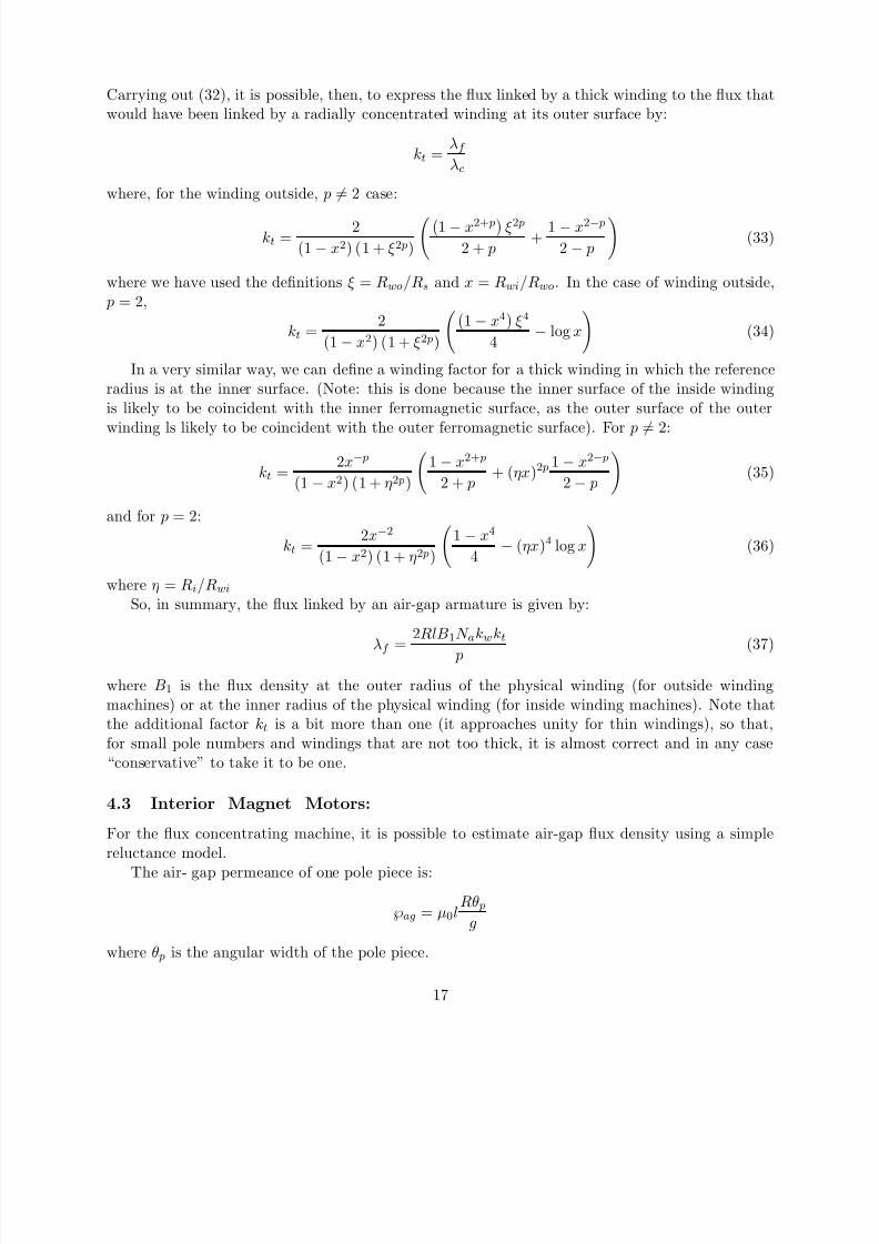
Carrying out (32), it is possible, then, to express the ux linked by a thick winding to the ux thatwould have been linked by a radially concentrated winding at its outer surface by:

λ f kt =λ c

where, for the winding outside, p = 2 case:

ξ2 p2 1 − x2+ p 1 − x2− p kt =

(1 − x2) (1 + ξ2 p) 2 + p +2 − p (33)

where we have used the denitions ξ = Rwo /R s and x = Rwi /R wo . In the case of winding outside, p = 2,

2 1 − x4 ξ4kt =

(1 − x2) (1 + ξ2 p) 4− log x (34)

In a very similar way, we can dene a winding factor for a thick winding in which the referenceradius is at the inner surface. (Note: this is done because the inner surface of the inside windingis likely to be coincident with the inner ferromagnetic surface, as the outer surface of the outer

winding ls likely to be coincident with the outer ferromagnetic surface). For p = 2:

2x − p 1 − x2+ p 1 − x2− p

kt =(1 − x2) (1 + η2 p) 2 + p + ( ηx)2 p

2 − p (35)

and for p = 2:2x − 2 1 − x4

kt = − (ηx)4 log x (36)(1 − x2) (1 + η2 p) 4

where η = R i /R wi

So, in summary, the ux linked by an air-gap armature is given by:

2RlB 1N a kw ktλf

= (37) p

where B1 is the ux density at the outer radius of the physical winding (for outside windingmachines) or at the inner radius of the physical winding (for inside winding machines). Note thatthe additional factor kt is a bit more than one (it approaches unity for thin windings), so that,for small pole numbers and windings that are not too thick, it is almost correct and in any case“conservative” to take it to be one.

4.3 Interior Magnet Motors:

For the ux concentrating machine, it is possible to estimate air-gap ux density using a simplereluctance model.

The air- gap permeance of one pole piece is:Rθ p

℘ag = µ0l g

where θ p is the angular width of the pole piece.

17



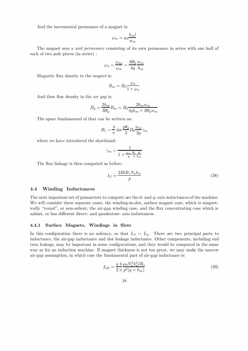
And the incremental permeance of a magnet is:

hm l ℘m = µ0 wm

The magnet sees a unit permeance consisting of its own permeance in series with one half of each of two pole pieces (in series) :

℘ag Rθ p wm℘u = =

℘m 4g hm

Magnetic ux density in the magnet is:℘uBm = B0 1 + ℘u

And then ux density in the air gap is:

2hm 2hm wmBg = Bm = B0Rθ p 4ghm + Rθ pwm

The space fundamental of that can be written as:

4 pθ p wmB1 = sin B0 γ mπ 2 2g

where we have introduced the shorthand:1

γ m =1 + wm θp R

g 4 h m

The ux linkage is then computed as before:

2RlB 1N a kwλ f = (38) p

4.4 Winding Inductances

The next important set of parameters to compute are the d- and q- axis inductances of the machine.We will consider three separate cases, the winding-in-slot, surface magnet case, which is magnetically “round”, or non-salient, the air-gap winding case, and the ux concentrating case which issalient, or has different direct- and quadrature- axis inductances.

4.4.1 Surface Magnets, Windings in Slots

In this conguration there is no saliency, so that Ld = Lq . There are two principal parts toinductance, the air-gap inductance and slot leakage inductance. Other components, including end

turn leakage, may be important in some congurations, and they would be computed in the sameway as for an induction machine. If magnet thickness is not too great, we may make the narrowair-gap assumption, in which case the fundamental part of air-gap inductance is:

q 4 µ0N 2k2 lR sLd1 = a w

2 π p2(g + hm )(39)

18



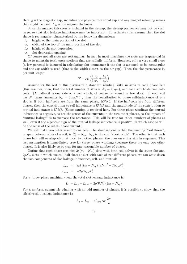
Here, g is the magnetic gap, including the physical rotational gap and any magnet retaining meansthat might be used. hm is the magnet thickness.

Since the magnet thickness is included in the air-gap, the air-gap permeance may not be verylarge, so that slot leakage inductance may be important. To estimate this, assume that the slotshape is rectangular, characterized by the following dimensions:

hs height of the main portion of the slot

ws

width of the top of the main portion of the slothd height of the slot depressionwd slot depression opening

Of course not all slots are rectangular: in fact in most machines the slots are trapezoidal inshape to maintain teeth cross-sections that are radially uniform. However, only a very small error(a few percent) is incurred in calculating slot permeance if the slot is assumed to be rectangularand the top width is used (that is the width closest to the air-gap). Then the slot permeance is,per unit length:

1 hs hdP = µ0 +3 ws wd

Assume for the rest of this discussion a standard winding, with m slots in each phase belt(this assumes, then, that the total number of slots is N s = 2 pqm), and each slot holds two half-coils. (A half-coil is one side of a coil which, of course, is wound in two slots). If each coilhas N c turns (meaning N a = 2 pmN c) , then the contribution to phase self-inductance of oneslot is, if both half-coils are from the same phase, 4 lP N 2. If the half-coils are from differentc

phases, then the contribution to self inductance is lP N 2 and the magnitude of the contribution toc

mutual inductance is lP N 2 . (Some caution is required here. For three phase windings the mutualc

inductance is negative, so are the senses of the currents in the two other phases, so the impact of “mutual leakage” is to increase the reactance. This will be true for other numbers of phases aswell, even if the algebraic sign of the mutual leakage inductance is positive, in which case so willbe the sense of the other- phase current.)

We will make two other assumptions here. The standard one is that the winding “coil throw”,or span between sides of a coil, is N s − N sp . N sp is the coil “short pitch”. The other is that each2 p

phase belt will overlap with, at most two other phases: the ones on either side in sequence. Thislast assumption is immediately true for three- phase windings (because there are only two otherphases. It is also likely to be true for any reasonable number of phases.

Noting that each phase occupies 2 p(m − N sp ) slots with both coil halves in the same slot and2 pN sp slots in which one coil half shares a slot with each of two different phases, we can write downthe two components of slot leakage inductance, self- and mutual:

Las = 2 pl (m − N sp ) (2N c)2 + 2 N sp N 2c

Lam = − 2 plN sp N 2c

For a three- phase machine, then, the total slot leakage inductance is:

La = Las

− Lam

= 2 plP N

2(4m

− N sp )c

For a uniform, symmetric winding with an odd number of phases, it is possible to show that theeffective slot leakage inductance is:

2π La = Las − 2Lam cos

q

19



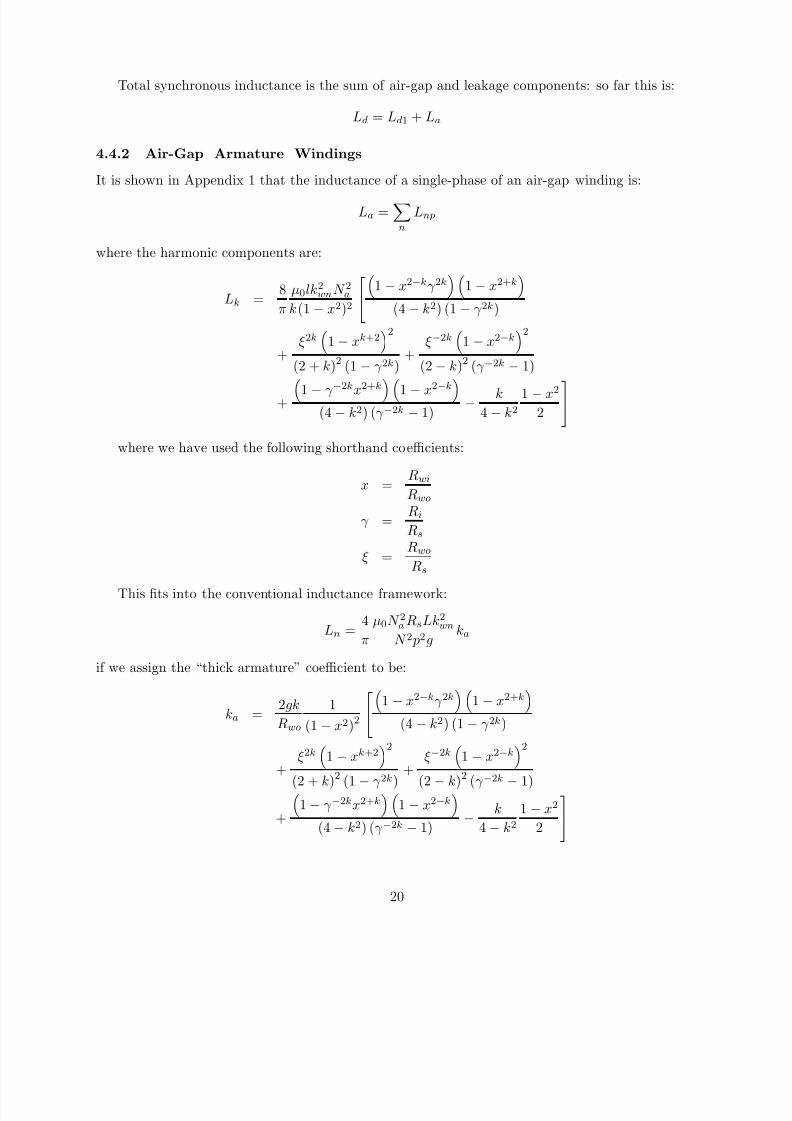
Total synchronous inductance is the sum of air-gap and leakage components: so far this is:

Ld = Ld1 + La

4.4.2 Air-Gap Armature Windings

It is shown in Appendix 1 that the inductance of a single-phase of an air-gap winding is:

La = Lnp n

where the harmonic components are:

8 µ0lk2 N 2 1 − x2− k γ 2k 1 − x2+ k

Lk = wn a π k(1 − x2)2 (4 − k2) (1 − γ 2k )

2

2

ξ2k ξ− 2k1 − xk+2 1 − x2− k

+ +(2 + k)2 (1 − γ 2k ) (2 − k)2 (γ − 2k − 1)

1 − γ − 2k 2+ k

x 1 − x2− k

k 1 − x2− (4 − k2) (γ − 2k − 1) 4 − k2 2

+

where we have used the following shorthand coefficients:

Rwi x =

Rwo

R iγ =R s

Rwo ξ =

R s

This ts into the conventional inductance framework:

4 µ0N 2R s Lk 2Ln = a wn ka2π N 2 p g

if we assign the “thick armature” coefficient to be:

2gk 1 1 − x2− k γ 2k 1 − x2+ k

ka = Rwo (1 − x2)2 (4 − k2) (1 − γ 2k )

2

2

ξ2k ξ− 2k1 − xk +2 1 − x2− k

+ +(2 + k)

2

(1 − γ 2k

) (2 − k)2

(γ − 2k

− 1) 1 − γ − 2k 2+ kx 1 − x2− k

k 1 − x2−

(4 − k2) (γ − 2k − 1) 4 − k2 2+

20



and k = np and g = R s − R i is the conventionally dened “air gap”. If the aspect ratio R i /R s isnot too far from unity, neither is ka . In the case of p = 2, the fundamental component of ka is:

4 1 − γ 4 γ 42gk 1 1 − x4 2γ 4 + x ξ4 1 − x4 2

ka =Rwo (1 − x2)2 8

−4 (1 − γ 4)

log x +ξ4 (1 − γ 4)

(log x)2 +16(1 − γ 4)

For a q-phase winding, a good approximation to the inductance is given by just the rst spaceharmonic term, or:

q 4 µ0N 2R s Lk 2Ld = a wn ka22 π n2 p g

4.4.3 Internal Magnet Motor

The permanent magnets will have an effect on reactance because the magnets are in the main uxpath of the armature. Further, they affect direct and quadrature reactances differently, so that themachine will be salient. Actually, the effect on the direct axis will likely be greater, so that thistype of machine will exhibit “negative” saliency: the quadrature axis reactance will be larger thanthe direct- axis reactance.

A full- pitch coil aligned with the direct axis of the machine would produce ux density:

µ0N a I B r =

2g 1 + Rθ p wm4g h m

Note that only the pole area is carrying useful ux, so that the space fundamental of radial uxdensity is:

µ0N a I 4 sin pθm

B1 =2g wm

2Rθ pπ 1 + h m 4g

Then, since the ux linked by the winding is:

2RlN a kw B1λ a = p

The d- axis inductance, including mutual phase coupling, is (for a q- phase machine):

q 4 µ0N 2Rlk 2 pθ pLd = a w γ m sin p22 π g 2

The quadrature axis is quite different. On that axis, the armature does not tend to push uxthrough the magnets, so they have only a minor effect. What effect they do have is due to the factthat the magnets produce a space in the active air- gap. Thus, while a full- pitch coil aligned withthe quadrature axis will produce an air- gap ux density:

µ0N I B r =

g

the space fundamental of that will be:

21



5

µ0N I 4 pθtB1 = 1 − sing π 2

where θt is the angular width taken out of the pole by the magnets.So that the expression for quadrature axis inductance is:

q 4 µ0N 2Rlk

2 pθtLq = a w 1 − sin p22 π g 2

Current Rating and Resistance

The last part of machine rating is its current capability. This is heavily inuenced by cooling methods, for the principal limit on current is the heating produced by resistive dissipation. Generally,it is possible to do rst-order design estimates by assuming a current density that can be handledby a particular cooling scheme. Then, in an air-gap winding:

N a I a = R2 − R2 θwe J awo wi 2

and note that, usually, the armature lls the azimuthal space in the machine:

2qθwe = 2 π

For a winding in slots, nearly the same thing is true: if the rectangular slot model holds true:

2qN a I a = N s hs ws J s

where we are using J s to note slot current density. Now, suppose we can characterize the total slotarea by a “space factor” λ s which is the ratio between total slot area and the annulus occupied bythe slots: for the rectangular slot model:

N s hs wsλ s =

π R2

− R2

wo wi where Rwi = R + hd and Rwo = Rwi + hs in a normal, stator outside winding. In this case, J a = J s λ s

and the two types of machines can be evaluated in the same way.It would seem apparent that one would want to make λ s as large as possible, to permit high

currents. The limit on this is that the magnetic teeth between the conductors must be able to carrythe air-gap ux, and making them too narrow would cause them to saturate. The peak of the timefundamental magnetic eld in the teeth is, for example,

2πR B t = B1 N s wt

where wt is the width of a stator tooth:

2π(R + hd )wt =N s

− ws

so thatB1B t ≈

1 − λ s

22



5.1 Resistance

Winding resistance may be estimated as the length of the stator conductor divided by its area andits conductivity. The length of the stator conductor is:

lc = 2 lN a f e

where the “end winding factor” f e is used to take into account the extra length of the end turns

(which is usually not negligible). The area of each turn of wire is, for an air-gap winding :

− R2θwe R2Aw = wo wi λw2 N a

where λw , the “packing factor” relates the area of conductor to the total area of the winding. Theresistance is then just:

4lN 2Ra = a

R2 − R2θwe wo wi λw σ

and, of course, σ is the conductivity of the conductor.For windings in slots the expression is almost the same, simply substituting the total slot area:

2qlN 2Ra = a

N s hs ws λw σ

The end turn allowance depends strongly on how the machine is made. One way of estimatingwhat it might be is to assume that the end turns follow a roughly circular path from one side of the machine to the other. The radius of this circle would be, very roughly, Rw /p , where Rw is theaverage radius of the winding: Rw ≈ (Rwo + Rwi )/ 2

Then the end-turn allowance would be:

πR wf e = 1 + pl

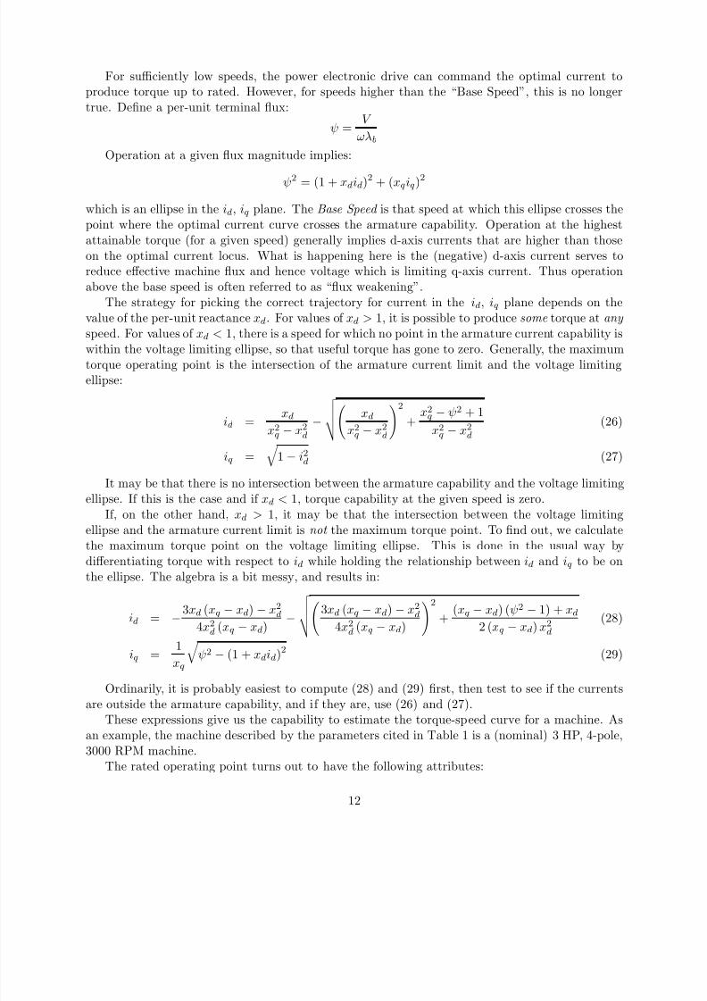
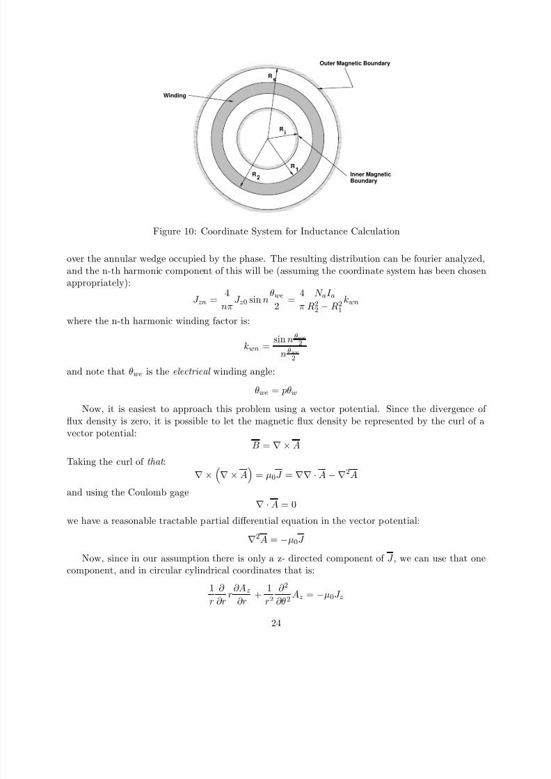
6 Appendix 1: Air-Gap Winding InductanceIn this appendix we use a simple two-dimensional model to estimate the magnetic elds and theninductances of an air-gap winding. The principal limiting assumption here is that the winding isuniform in the ̂ z direction, which means it is long in comparison with its radii. This is generally nottrue, nevertheless the answers we will get are not too far from being correct. The style of analysisused here can be carried into a three-dimensional, or quasi-three dimensional domain to get muchmore precise answers, at the expense of a very substantial increase in complexity.

The coordinate system to be used is shown in Figure 10. To maintain generality we have fourradii: R i and R s are ferromagnetic boundaries, and would of course correspond with the machineshaft and the stator core. The winding itself is carried between radii R1 and R2, which correspond

with radii Rwi and Rwo in the body of the text. It is assumed that the armature is carrying acurrent in the z- direction, and that this current is uniform in the radial dimension of the armature.If a single phase of the armature is carrying current, that current will be:

N a I aJ z 0 =

θwe R2

2 − R22 1

23



0 0 0 0 0 0 0 0 0 0 0 0 0 0 0 00 0 0 0 0 0 0 0 0 0 0 0 0 0 0 00 0 0 0 0 0 0 0 0 0 0 0 0 0 0 00 0 0 0 0 0 0 0 0 0 0 0 0 0 0 00 0 0 0 0 0 0 0 0 0 0 0 0 0 0 00 0 0 0 0 0 0 0 0 0 0 0 0 0 0 00 0 0 0 0 0 0 0 0 0 0 0 0 0 0 00 0 0 0 0 0 0 0 0 0 0 0 0 0 0 00 0 0 0 0 0 0 0 0 0 0 0 0 0 0 00 0 0 0 0 0 0 0 0 0 0 0 0 0 0 00 0 0 0 0 0 0 0 0 0 0 0 0 0 0 00 0 0 0 0 0 0 0 0 0 0 0 0 0 0 00 0 0 0 0 0 0 0 0 0 0 0 0 0 0 00 0 0 0 0 0 0 0 0 0 0 0 0 0 0 00 0 0 0 0 0 0 0 0 0 0 0 0 0 0 00 0 0 0 0 0 0 0 0 0 0 0 0 0 0 00 0 0 0 0 0 0 0 0 0 0 0 0 0 0 00 0 0 0 0 0 0 0 0 0 0 0 0 0 0 00 0 0 0 0 0 0 0 0 0 0 0 0 0 0 00 0 0 0 0 0 0 0 0 0 0 0 0 0 0 00 0 0 0 0 0 0 0 0 0 0 0 0 0 0 00 0 0 0 0 0 0 0 0 0 0 0 0 0 0 00 0 0 0 0 0 0 0 0 0 0 0 0 0 0 00 0 0 0 0 0 0 0 0 0 0 0 0 0 0 00 0 0 0 0 0 0 0 0 0 0 0 0 0 0 00 0 0 0 0 0 0 0 0 0 0 0 0 0 0 00 0 0 0 0 0 0 0 0 0 0 0 0 0 0 00 0 0 0 0 0 0 0 0 0 0 0 0 0 0 00 0 0 0 0 0 0 0 0 0 0 0 0 0 0 0

Outer Magnetic Boundary

Winding

Inner MagneticBoundary

1 1 1 1 1 1 1 1 1 1 1 1 1 1 1 1 11 1 1 1 1 1 1 1 1 1 1 1 1 1 1 1 11 1 1 1 1 1 1 1 1 1 1 1 1 1 1 1 11 1 1 1 1 1 1 1 1 1 1 1 1 1 1 1 11 1 1 1 1 1 1 1 1 1 1 1 1 1 1 1 11 1 1 1 1 1 1 1 1 1 1 1 1 1 1 1 11 1 1 1 1 1 1 1 1 1 1 1 1 1 1 1 11 1 1 1 1 1 1 1 1 1 1 1 1 1 1 1 11 1 1 1 1 1 1 1 1 1 1 1 1 1 1 1 11 1 1 1 1 1 1 1 1 1 1 1 1 1 1 1 11 1 1 1 1 1 1 1 1 1 1 1 1 1 1 1 11 1 1 1 1 1 1 1 1 1 1 1 1 1 1 1 11 1 1 1 1 1 1 1 1 1 1 1 1 1 1 1 11 1 1 1 1 1 1 1 1 1 1 1 1 1 1 1 11 1 1 1 1 1 1 1 1 1 1 1 1 1 1 1 11 1 1 1 1 1 1 1 1 1 1 1 1 1 1 1 11 1 1 1 1 1 1 1 1 1 1 1 1 1 1 1 11 1 1 1 1 1 1 1 1 1 1 1 1 1 1 1 11 1 1 1 1 1 1 1 1 1 1 1 1 1 1 1 11 1 1 1 1 1 1 1 1 1 1 1 1 1 1 1 11 1 1 1 1 1 1 1 1 1 1 1 1 1 1 1 11 1 1 1 1 1 1 1 1 1 1 1 1 1 1 1 11 1 1 1 1 1 1 1 1 1 1 1 1 1 1 1 11 1 1 1 1 1 1 1 1 1 1 1 1 1 1 1 11 1 1 1 1 1 1 1 1 1 1 1 1 1 1 1 11 1 1 1 1 1 1 1 1 1 1 1 1 1 1 1 11 1 1 1 1 1 1 1 1 1 1 1 1 1 1 1 11 1 1 1 1 1 1 1 1 1 1 1 1 1 1 1 11 1 1 1 1 1 1 1 1 1 1 1 1 1 1 1 1

0 0 0 0 0 0 0 0 0 0 0 00 0 0 0 0 0 0 0 0 0 0 00 0 0 0 0 0 0 0 0 0 0 00 0 0 0 0 0 0 0 0 0 0 00 0 0 0 0 0 0 0 0 0 0 00 0 0 0 0 0 0 0 0 0 0 00 0 0 0 0 0 0 0 0 0 0 00 0 0 0 0 0 0 0 0 0 0 00 0 0 0 0 0 0 0 0 0 0 00 0 0 0 0 0 0 0 0 0 0 00 0 0 0 0 0 0 0 0 0 0 00 0 0 0 0 0 0 0 0 0 0 0

1 1 1 1 1 1 1 1 1 1 1 11 1 1 1 1 1 1 1 1 1 1 11 1 1 1 1 1 1 1 1 1 1 11 1 1 1 1 1 1 1 1 1 1 11 1 1 1 1 1 1 1 1 1 1 11 1 1 1 1 1 1 1 1 1 1 11 1 1 1 1 1 1 1 1 1 1 11 1 1 1 1 1 1 1 1 1 1 11 1 1 1 1 1 1 1 1 1 1 11 1 1 1 1 1 1 1 1 1 1 11 1 1 1 1 1 1 1 1 1 1 11 1 1 1 1 1 1 1 1 1 1 1

i

R 1R 2

R s

R

Figure 10: Coordinate System for Inductance Calculation

over the annular wedge occupied by the phase. The resulting distribution can be fourier analyzed,

and the n-th harmonic component of this will be (assuming the coordinate system has been chosenappropriately):4 θwe 4 N a I aJ zn = J z 0 sin n =

2 − R2 kwn nπ 2 π R2

1

where the n-th harmonic winding factor is:

sin n θwe

kwn = θwe

2

n 2

and note that θwe is the electrical winding angle:

θwe = pθw

Now, it is easiest to approach this problem using a vector potential. Since the divergence of ux density is zero, it is possible to let the magnetic ux density be represented by the curl of avector potential:

B = ∇ × A

Taking the curl of that :∇ × ∇ × A

and using the Coulomb gage∇ · A = 0

we have a reasonable tractable partial differential equation in the vector potential:

∇2A = − µ0J

Now, since in our assumption there is only a z- directed component of J , we can use that onecomponent, and in circular cylindrical coordinates that is:

1 ∂ ∂A z 1 ∂ 2r + Az = − µ0J z

r 2 ∂θ2r ∂r ∂r

24

= µ0J = ∇∇ · A − ∇ 2A



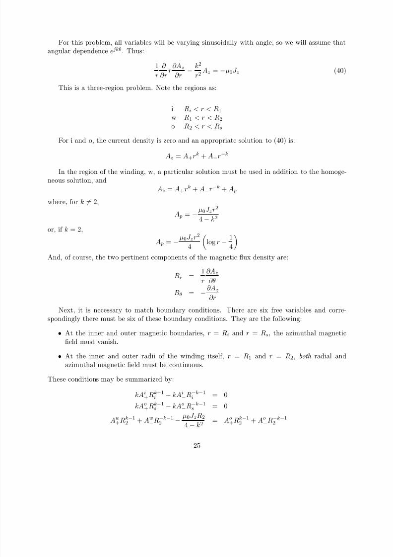
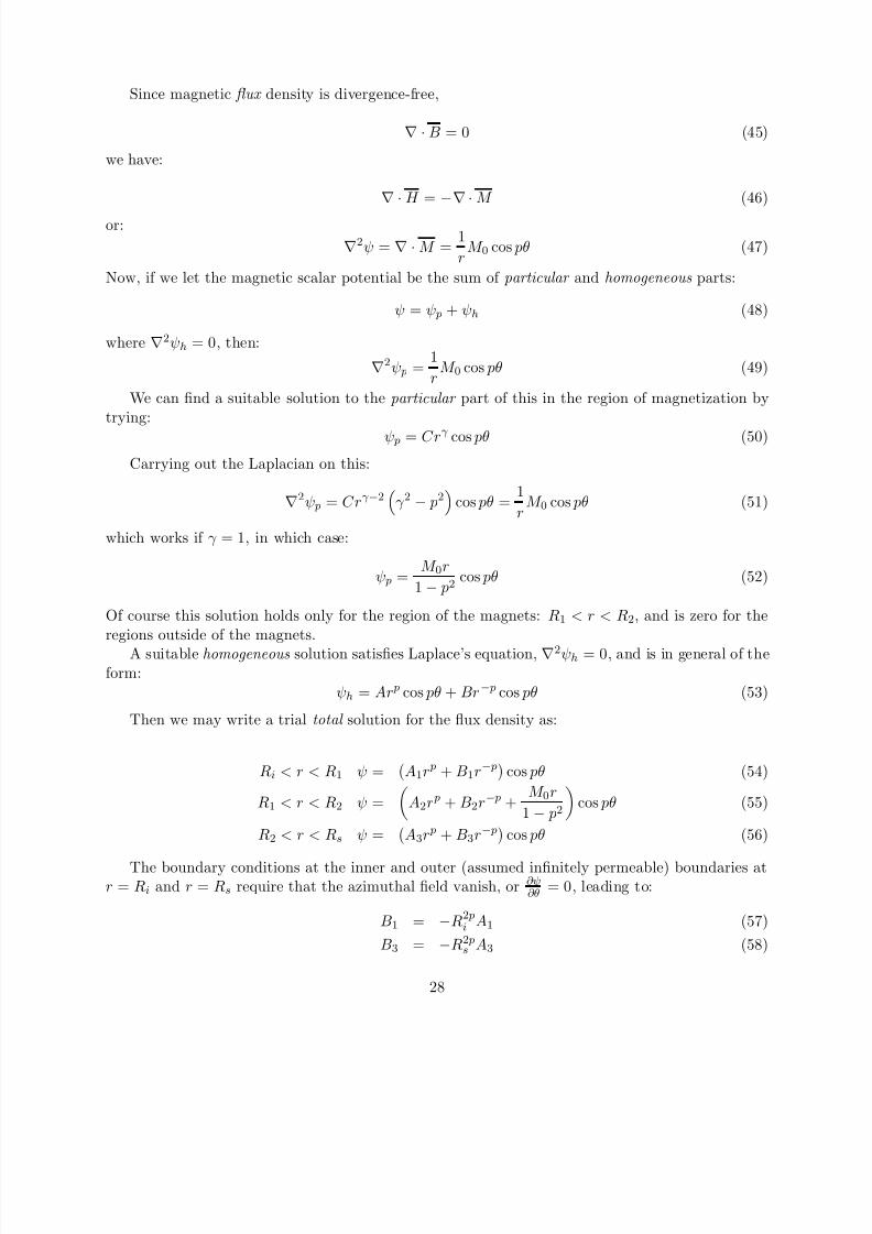
For this problem, all variables will be varying sinusoidally with angle, so we will assume thatangular dependence e jkθ . Thus:

1 ∂ ∂A z k2r − Az = − µ0J z (40)

r ∂r ∂r r 2

This is a three-region problem. Note the regions as:

i R i < r < R1w R1 < r < R2o R2 < r < R s

For i and o, the current density is zero and an appropriate solution to (40) is:

− kAz = A+ r k + A− r

In the region of the winding, w, a particular solution must be used in addition to the homogeneous solution, and

− kAz = A+ r k + A− r + A p

where, for k = 2,µ0J z r 2

A p = −4 − k2

or, if k = 2,µ0J z r 2 1

A p = − log r −4 4

And, of course, the two pertinent components of the magnetic ux density are:

1 ∂A zB r =r ∂θ

∂A zBθ = − ∂r

Next, it is necessary to match boundary conditions. There are six free variables and correspondingly there must be six of these boundary conditions. They are the following:

• At the inner and outer magnetic boundaries, r = R i and r = R s , the azimuthal magneticeld must vanish.

• At the inner and outer radii of the winding itself, r = R1 and r = R2, both radial andazimuthal magnetic eld must be continuous.

These conditions may be summarized by:

Rk − 1 R − k − 1kA i − kA i = 0+ i − i

Rk − 1 R − k − 1kAo − kAo = 0+ s − s

Aw Rk − 1 + Aw R − k − 1 µ0J z R2− = Ao Rk − 1 + Ao R − k − 1+ 2 − 2 4 − k2 + 2 − 2

25



+

− kAw Rk − 1 + kAw R − k − 1 2µ0J z R2 = − kAo Rk − 1 + kAo R − k − 1+ 2 − 2 +

4 − k2 + 2 − 2

Aw Rk − 1 + Aw R − k − 1 µ0J z R1− = Ai Rk − 1 + Ai R − k − 1+ 1 − 1 4 − k2 + 1 − 1

Rk − 1 R − k − 1 2µ0J z R1 Rk − 1 R − k − 1− kAw + kAw + 1 − 1 +

4 − k2 = − kA+i

1 + kA −

i 1

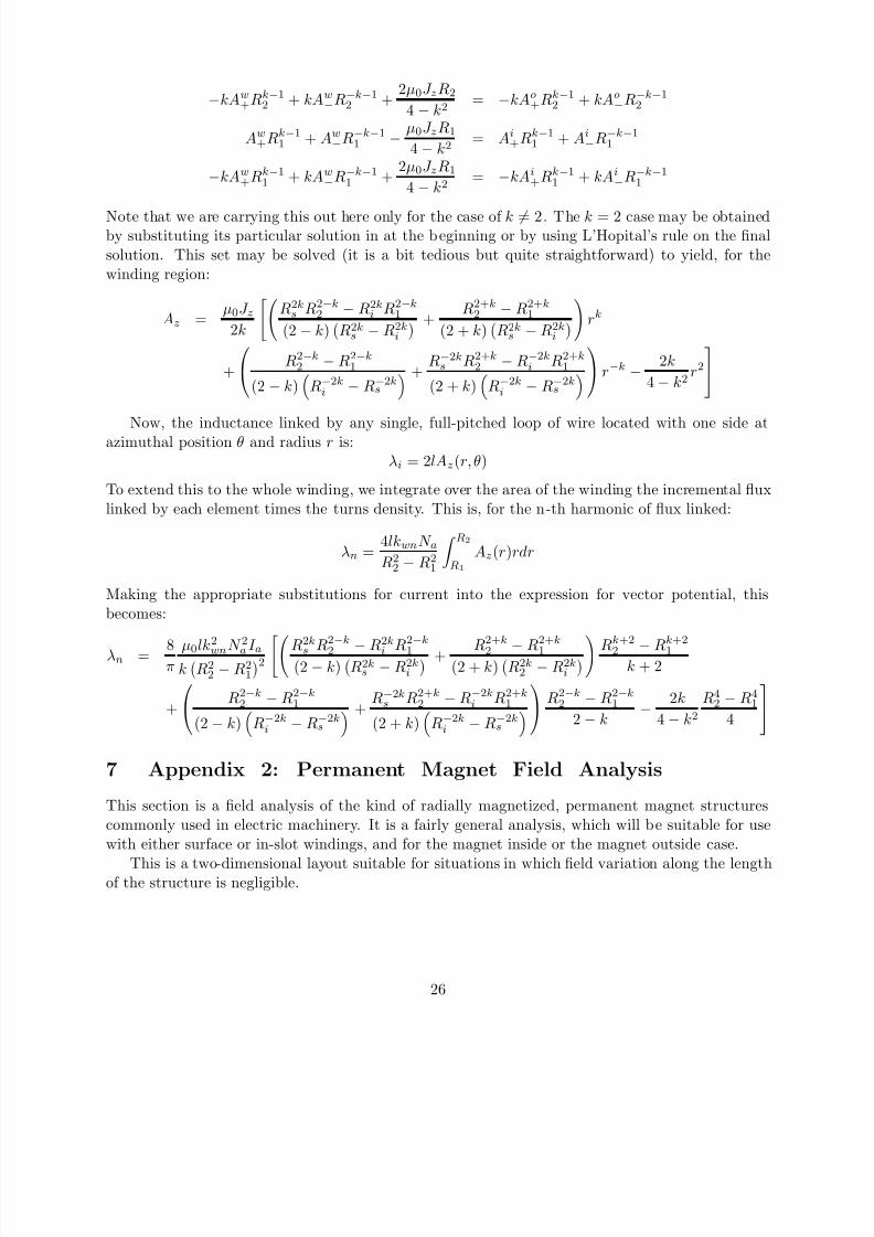
Note that we are carrying this out here only for the case of k = 2. The k = 2 case may be obtainedby substituting its particular solution in at the beginning or by using L’Hopital’s rule on the nalsolution. This set may be solved (it is a bit tedious but quite straightforward) to yield, for thewinding region:

µ0J z R2k R2− k − R2k R2− k R2+ k

− R2+ k

Az = s 2 i 1 2 1 k

+

r

2k (2 − k) R2k − R2k (2 + k) R2k − R2k s i s i

R2− k − R2− k R − 2k R2+ k

− R − 2k R2+ k 2k 22 1 s 2 i 1 − k+ + r − r

4 − k2(2 − k) R − 2k − R − 2k (2 + k) R − 2k

− R − 2k s i si

Now, the inductance linked by any single, full-pitched loop of wire located with one side atazimuthal position θ and radius r is:

λ i = 2 lAz (r, θ)

To extend this to the whole winding, we integrate over the area of the winding the incremental uxlinked by each element times the turns density. This is, for the n-th harmonic of ux linked:

R 24lkwn N aλn =2 − R2 Az (r )rdr

R21 R 1

Making the appropriate substitutions for current into the expression for vector potential, thisbecomes:

R2+ k

− R2+ k

Rk +2

− Rk+2

λn = 8 µ 0lk2

N 2

s 2 1wn a I a R2k

R2− k

− R i 2k

R2− k

2 1 2 1

2 − R2 2 (2 − k) R2k − R2k (2 + k) R2k − R2k k + 2π k R21 s i 2 i

R2− k − R2− k R − 2k R2+ k

− R − 2k R2+ k R2− k − R2− k

2 − R42k R412 1 s 2 i 1 2 1+ + −

(2 − k) R − 2k − R − 2k (2 + k) R − 2k

− R − 2k 2 − k 4 − k2 4s i si

7 Appendix 2: Permanent Magnet Field Analysis

This section is a eld analysis of the kind of radially magnetized, permanent magnet structurescommonly used in electric machinery. It is a fairly general analysis, which will be suitable for usewith either surface or in-slot windings, and for the magnet inside or the magnet outside case.

This is a two-dimensional layout suitable for situations in which eld variation along the lengthof the structure is negligible.

26



0 0 0 0 0 0 0 0 0 0 0 0 0 0 0 00 0 0 0 0 0 0 0 0 0 0 0 0 0 0 00 0 0 0 0 0 0 0 0 0 0 0 0 0 0 00 0 0 0 0 0 0 0 0 0 0 0 0 0 0 00 0 0 0 0 0 0 0 0 0 0 0 0 0 0 00 0 0 0 0 0 0 0 0 0 0 0 0 0 0 00 0 0 0 0 0 0 0 0 0 0 0 0 0 0 00 0 0 0 0 0 0 0 0 0 0 0 0 0 0 00 0 0 0 0 0 0 0 0 0 0 0 0 0 0 00 0 0 0 0 0 0 0 0 0 0 0 0 0 0 00 0 0 0 0 0 0 0 0 0 0 0 0 0 0 00 0 0 0 0 0 0 0 0 0 0 0 0 0 0 00 0 0 0 0 0 0 0 0 0 0 0 0 0 0 00 0 0 0 0 0 0 0 0 0 0 0 0 0 0 00 0 0 0 0 0 0 0 0 0 0 0 0 0 0 00 0 0 0 0 0 0 0 0 0 0 0 0 0 0 00 0 0 0 0 0 0 0 0 0 0 0 0 0 0 00 0 0 0 0 0 0 0 0 0 0 0 0 0 0 00 0 0 0 0 0 0 0 0 0 0 0 0 0 0 00 0 0 0 0 0 0 0 0 0 0 0 0 0 0 00 0 0 0 0 0 0 0 0 0 0 0 0 0 0 00 0 0 0 0 0 0 0 0 0 0 0 0 0 0 00 0 0 0 0 0 0 0 0 0 0 0 0 0 0 00 0 0 0 0 0 0 0 0 0 0 0 0 0 0 00 0 0 0 0 0 0 0 0 0 0 0 0 0 0 00 0 0 0 0 0 0 0 0 0 0 0 0 0 0 00 0 0 0 0 0 0 0 0 0 0 0 0 0 0 00 0 0 0 0 0 0 0 0 0 0 0 0 0 0 00 0 0 0 0 0 0 0 0 0 0 0 0 0 0 0

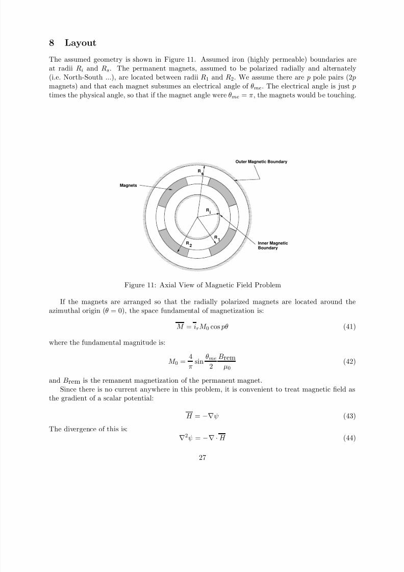
8 Layout

The assumed geometry is shown in Figure 11. Assumed iron (highly permeable) boundaries areat radii R i and R s . The permanent magnets, assumed to be polarized radially and alternately(i.e. North-South ...), are located between radii R1 and R2. We assume there are p pole pairs (2 p magnets) and that each magnet subsumes an electrical angle of θme . The electrical angle is just p times the physical angle, so that if the magnet angle were θme = π, the magnets would be touching.

Outer Magnetic Boundary

Magnets

1 1 1 1 1 1 1 1 1 1 1 1 1 1 1 1 11 1 1 1 1 1 1 1 1 1 1 1 1 1 1 1 11 1 1 1 1 1 1 1 1 1 1 1 1 1 1 1 11 1 1 1 1 1 1 1 1 1 1 1 1 1 1 1 11 1 1 1 1 1 1 1 1 1 1 1 1 1 1 1 11 1 1 1 1 1 1 1 1 1 1 1 1 1 1 1 11 1 1 1 1 1 1 1 1 1 1 1 1 1 1 1 11 1 1 1 1 1 1 1 1 1 1 1 1 1 1 1 11 1 1 1 1 1 1 1 1 1 1 1 1 1 1 1 11 1 1 1 1 1 1 1 1 1 1 1 1 1 1 1 11 1 1 1 1 1 1 1 1 1 1 1 1 1 1 1 11 1 1 1 1 1 1 1 1 1 1 1 1 1 1 1 11 1 1 1 1 1 1 1 1 1 1 1 1 1 1 1 11 1 1 1 1 1 1 1 1 1 1 1 1 1 1 1 11 1 1 1 1 1 1 1 1 1 1 1 1 1 1 1 11 1 1 1 1 1 1 1 1 1 1 1 1 1 1 1 11 1 1 1 1 1 1 1 1 1 1 1 1 1 1 1 11 1 1 1 1 1 1 1 1 1 1 1 1 1 1 1 11 1 1 1 1 1 1 1 1 1 1 1 1 1 1 1 11 1 1 1 1 1 1 1 1 1 1 1 1 1 1 1 11 1 1 1 1 1 1 1 1 1 1 1 1 1 1 1 11 1 1 1 1 1 1 1 1 1 1 1 1 1 1 1 11 1 1 1 1 1 1 1 1 1 1 1 1 1 1 1 11 1 1 1 1 1 1 1 1 1 1 1 1 1 1 1 11 1 1 1 1 1 1 1 1 1 1 1 1 1 1 1 11 1 1 1 1 1 1 1 1 1 1 1 1 1 1 1 11 1 1 1 1 1 1 1 1 1 1 1 1 1 1 1 11 1 1 1 1 1 1 1 1 1 1 1 1 1 1 1 11 1 1 1 1 1 1 1 1 1 1 1 1 1 1 1 1

0 0 0 0 0 0 0 0 0 0 0 00 0 0 0 0 0 0 0 0 0 0 00 0 0 0 0 0 0 0 0 0 0 00 0 0 0 0 0 0 0 0 0 0 00 0 0 0 0 0 0 0 0 0 0 00 0 0 0 0 0 0 0 0 0 0 00 0 0 0 0 0 0 0 0 0 0 00 0 0 0 0 0 0 0 0 0 0 00 0 0 0 0 0 0 0 0 0 0 00 0 0 0 0 0 0 0 0 0 0 00 0 0 0 0 0 0 0 0 0 0 00 0 0 0 0 0 0 0 0 0 0 0

1 1 1 1 1 1 1 1 1 1 1 11 1 1 1 1 1 1 1 1 1 1 11 1 1 1 1 1 1 1 1 1 1 11 1 1 1 1 1 1 1 1 1 1 11 1 1 1 1 1 1 1 1 1 1 11 1 1 1 1 1 1 1 1 1 1 11 1 1 1 1 1 1 1 1 1 1 11 1 1 1 1 1 1 1 1 1 1 11 1 1 1 1 1 1 1 1 1 1 11 1 1 1 1 1 1 1 1 1 1 11 1 1 1 1 1 1 1 1 1 1 11 1 1 1 1 1 1 1 1 1 1 1

Boundary

R s

R i

R 1R 2 Inner Magnetic

Figure 11: Axial View of Magnetic Field Problem

If the magnets are arranged so that the radially polarized magnets are located around theazimuthal origin ( θ = 0), the space fundamental of magnetization is:

M = i r M 0 cos pθ (41)

where the fundamental magnitude is:

4 θme BremM 0 = sin (42)π 2 µ0

and Brem is the remanent magnetization of the permanent magnet.Since there is no current anywhere in this problem, it is convenient to treat magnetic eld as

the gradient of a scalar potential:

H = −∇ ψ (43)

The divergence of this is:∇

2ψ = −∇ · H (44)

27



Since magnetic ux density is divergence-free,

∇ · B = 0 (45)

we have:

∇ · H = −∇ · M (46)

or:∇

2ψ = ∇ · M =1

M 0 cos pθ (47)r

Now, if we let the magnetic scalar potential be the sum of particular and homogeneous parts:

ψ = ψ p + ψh (48)

where ∇ 2ψh = 0, then:∇

2ψ p =1

M 0 cos pθ (49)r

We can nd a suitable solution to the particular part of this in the region of magnetization bytrying:

ψ p = Cr γ cos pθ (50)Carrying out the Laplacian on this:

∇2ψ p = Cr γ − 2 γ 2 − p 2 cos pθ =

1M 0 cos pθ (51)

r

which works if γ = 1, in which case:

M 0r ψ p = cos pθ (52)

1 − p2

Of course this solution holds only for the region of the magnets: R1 < r < R2, and is zero for theregions outside of the magnets.

A suitable homogeneous solution satises Laplace’s equation, ∇ 2ψh = 0, and is in general of theform:

ψh = Ar p cos pθ + Br − p cos pθ (53)

Then we may write a trial total solution for the ux density as:

R i < r < R1 ψ = A1r p + B1r − p

cos pθ (54)

R1 < r < R2 ψ =

A2r p + B2r − p +M 0r

1 − p2

cos pθ (55)

R2 < r < R s ψ = A3r p + B3r − p

cos pθ (56)

The boundary conditions at the inner and outer (assumed innitely permeable) boundaries atr = R i and r = R s require that the azimuthal eld vanish, or ∂ψ = 0, leading to:∂θ

B1 = − R i 2 pA1 (57)

B3 = − R2 pA3 (58)s

28



At the magnet inner and outer radii, H θ and B r must be continuous. These are:

1 ∂ψ H θ = − (59)

r ∂θ ∂ψ

B r = µ0 − + M r (60)∂r

These become, at r = R1:

2 pR− p− 1− pA1 R p− 1 − R = − p A2R p− 1 + B2R

− p− 1 − pM 0 (61)1 i 1 1 1 1 − p2

2 pR− p− 1− pA1 R p− 1 + R = − p A2R p− 1 − B2R

− p− 1 −M 0 + M 0 (62)1 i 1 1 1 1 − p2

and at r = R2:

− pA3 R p− 1 − R2 pR− p− 1 = − p A2R p− 1 + B2R

− p− 1 − pM 0 (63)2 s 2 2 2 1 − p2

− pA3 R p− 1 + R2 pR− p− 1 = − p A2R p− 1 − B2R

− p− 1 −M 0 + M 0 (64)2 s 2 2 2 1 − p2

Some small-time manipulation of these yields:

A1 1 − R2 pR− pR p

= A2R p 11 + B2R− p

+ R1M 0 (65)i 1 1 − p2

A1 1 + R2 pR− pR p

= A2R p 11 − B2R− p

+ pR1M 0 (66)i 1 1 − p2

R p = A2R p

2A3 2 − R2 pR− p

2 + B2R− p

+ R2M 0 (67)s 2 1 − p2

A3 R p = A2R p

22 + R2 pR− p

2 − B2R− p

+ pR2M 0 (68)s 2 1 − p2

Taking sums and differences of the rst and second and then third and fourth of these we obtain:

2A1R p = 2 A2R p 1 + p

(69)1 1 + R1M 0 1 − p2

2A1R i 2 pR

− p − 2B2R

− p + R1M 0

p − 1= (70)1 1 1 − p2

2A3R p = 2 A2R p 1 + p

(71)2 2 + R2M 0 1 − p2

2A3R2 pR− p

= − 2B2R− p

+ R2M 0 p − 1

(72)s 2 2 1 − p2

and then multiplying through by appropriate factors ( R p and R p

1) and then taking sums and2

differences of these ,

(A1 − A3) R p 2 − R2R p

1R p = ( R1R p

1)M 0 p + 1

(73)2 2 1 − p2

A1R i 2 p

− A3R2 p R− pR

− p R1R

− p − R2R

− p M 0 p − 1

= (74)s 1 2 2 1 2 1 − p2

29



Dividing through by the appropriate groups: pR1R2 − R2R p

1 M 0 1 + pA1 − A3 = pR1R p

2 1 − p2 (75)2

− p − p

A1R i 2 p 2 p R1R2 − R2R1 M 0 p − 1

(76)− A3R s = − p − p 2 1 − p2R1 R2

and then, by multiplying the top equation by R2 p and subtracting:s

p − p − p

A1 R2 p − R i 2 p

R1R2 − R2R p 1 M 0 1 + p

R2 p R1R2 − R2R1 M 0 p − 1(77)= −s p sR1R p

2 1 − p2 − p − p 2 1 − p22 R1 R2

This is readily solved for the eld coefficients A1 and A3:

M 0 p + 1 1− p 1− p R2 p p − 1 1+ p

− R1A1 = − 2 p

− R i 2 p

R1 − R2 + R21+ p

(78)s 2 R s p2 − 1 p2 − 1

M 0 1 1− p 1− p R i

2 p 1 1+ p 1+ pA3 = − − R2 − − R1 (79)2 p

− R i

2 p

1 − pR1 1 + p

R2

2 R s

Now, noting that the scalar potential is, in region 1 (radii less than the magnet),

ψ = A1(r p − R2 pr − p)cos pθ r < R 1i

ψ = A3(r p − R2 pr − p)cos pθ r > R 2s

and noting that p( p + 1) / ( p2 − 1) = p/ ( p − 1) and p( p − 1)/ ( p2 − 1) = p/ ( p + 1), magnetic eld is:

r < R 1 (80)M 0 p 1− p 1− p

R2 p p 1+ p 1+ p

p−

1 + R i 2 p

r −

p−

1 − R2 + − R1 r cos pθ s R2H r = 2 p − R i

2 p p − 1 R12 R s p + 1

r > R 2 (81)M 0 p 1− p 1− p

R i 2 p p 1+ p 1+ p − R2 + R2 − R1 r p− 1 + R2 pr − p− 1 cos pθ H r =

2 p − R i

2 p p − 1R1 p + 1 s

2 R s

The case of p = 1 appears to be a bit troublesome here, but is easily handled by noting that:

p 1− p 1− p R2lim R1 − R2 = log p→ 1 p − 1 R1

Now: there are a number of special cases to consider.For the iron-free case, R i → 0 and R2 → ∞ , this becomes, simply, for r < R 1:

p 1− pH r =M 0 R1

1− p r p− 1 cos pθ (82)− R22 p − 1

30



Note that for the case of p = 1, the limit of this is

M 0 R2H r = log cos θ 2 R1

and for r > R2:

M 0 pR

p+1− R

p+1 −

( p+1) cos pθ H r = 2 p + 1 2 1 r

For the case of a machine with iron boundaries and windings in slots, we are interested in theelds at the boundaries. In such a case, usually, either R i = R1 or R s = R2. The elds are:at the outer boundary: r = R s :

R p− 1 pR p+1 − R p+1 +

pR i

2 p 1− p 1− pH r = M 0 2 ps

− R2 cos pθ 2 1R s − R i

2 p p + 1 p − 1R1

or at the inner boundary: r = R i :

R p− 1

H r = M 0 2 pi p

R p+1

− R p+1 p

R2 p 1− p

− R2 cos pθ 2 1R s − R i 2 p p + 1 + p − 1 s R1

1− p

31

permanent magnet brushless dc

Documents