rc helicopter redesign - welcome | georgia tech … · rc helicopter redesign ... several crucial...

Jason Park Karthika PV. Colin Stieglitz 4-16-2014

ME 4041

RC Helicopter Redesign Final Report

of 53

Contents

INTRODUCTION ............................................................................................................................... 2

OBJECTIVES ..................................................................................................................................... 2

MODELING ...................................................................................................................................... 3

1. HEAD ASSEMBLY ...................................................................................................................... 3

2. MID-BODY ASSEMBLY ............................................................................................................ 13

3. TAIL ASSEMBLY ...................................................................................................................... 16

4. LANDING GEAR ...................................................................................................................... 23

ANALYSIS AND VERIFICATION ....................................................................................................... 25

5. HEAD ASSEMBLY .................................................................................................................... 25

6. TAIL ASSEMBLY ...................................................................................................................... 33

7. LANDING ASSEMBLY .............................................................................................................. 39

SUMMARY AND FUTURE WORKS ................................................................................................. 52

of 53

INTRODUCTION

Our group, consisting of Karthika PV, Colin Steiglitz, and Jason Park, chose to redesign a remote

control (RC) helicopter. We chose this project due to the fact that 2 out of the 3 group

members bought and returned the product for problems that we feel could have been avoided

through simple design changes. There is also a large market for these products.

There are two main areas of which need improvements: structural integrity and

maneuverability. Structural integrity can be an issue in the event of a collision or hard landing.

Also, there have been problems with balancing a hovering helicopter, especially after a “crash”.

Often, repairs are needed. Strategic structural improvements could greatly lengthen the

lifespan of these devices. Structural improvements also increase the stability of the RC

helicopter. Other alterations involve analyzing the aerodynamics of the rotors, which is a

complex design problem. A redesign of the rotors could increase maneuverability and stability

during flight.

There are many specified markets for different cost ranges, and therefore, different

features. The major markets we are designing for are the general hobbyists, enthusiasts, and

drone-related markets. We feel as though these different markets will all benefit from the

consequences of simple design changes.

OBJECTIVES

The objective of this project was to analyze and redesign a RC helicopter. First, a precise

computer aided design (CAD) model was developed including the crucial features. This was

done by physically measuring the dimensions and angles for each part. Accurate material

properties were found and assigned to the model. A computer aided structural analysis of

of 53

several crucial components was completed using Siemens NX software. The main components

for analysis included: the rotors, rotor connector, landing assembly, and tail assembly. The

structural analysis was verified with hand calculations. Depending on the results of the hand

calculations, the relevant parts were redesigned. In addition, a qualitative computational fluid

dynamics (CFD) analysis was performed on the rotors. This will be utilized for further redesign

in the future.

MODELING

1. HEAD ASSEMBLY

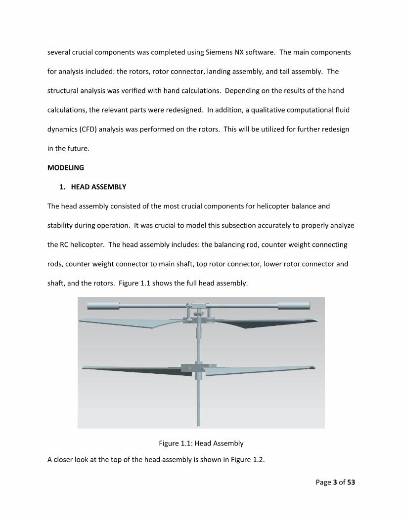
The head assembly consisted of the most crucial components for helicopter balance and

stability during operation. It was crucial to model this subsection accurately to properly analyze

the RC helicopter. The head assembly includes: the balancing rod, counter weight connecting

rods, counter weight connector to main shaft, top rotor connector, lower rotor connector and

shaft, and the rotors. Figure 1.1 shows the full head assembly.

Figure 1.1: Head Assembly

A closer look at the top of the head assembly is shown in Figure 1.2.

of 53

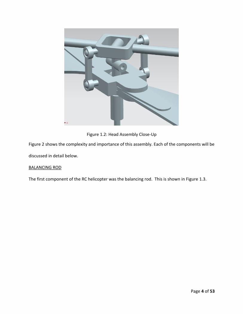
Figure 1.2: Head Assembly Close-Up

Figure 2 shows the complexity and importance of this assembly. Each of the components will be

discussed in detail below.

BALANCING ROD

The first component of the RC helicopter was the balancing rod. This is shown in Figure 1.3.

of 53

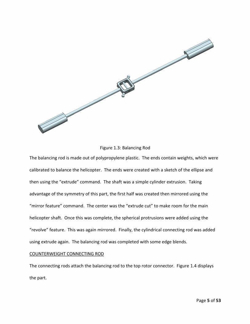
Figure 1.3: Balancing Rod

The balancing rod is made out of polypropylene plastic. The ends contain weights, which were

calibrated to balance the helicopter. The ends were created with a sketch of the ellipse and

then using the “extrude” command. The shaft was a simple cylinder extrusion. Taking

advantage of the symmetry of this part, the first half was created then mirrored using the

“mirror feature” command. The center was the “extrude cut” to make room for the main

helicopter shaft. Once this was complete, the spherical protrusions were added using the

“revolve” feature. This was again mirrored. Finally, the cylindrical connecting rod was added

using extrude again. The balancing rod was completed with some edge blends.

COUNTERWEIGHT CONNECTING ROD

The connecting rods attach the balancing rod to the top rotor connector. Figure 1.4 displays

the part.

of 53

Figure 1.4: Connecting Rod

The connecting rod was created with a sketch. First, a straight line was drawn, which defined

the distance between the center of the two holes. Two concentric circles were drawn at each

end of the line. Next, the “offset” command was used to define the boundary of the straight

bar between the holes. The “quick trim” command was utilized to edit the sketch to the

desired shape. Once the desired shape was attained, a simple extrusion completed the part.

Counterweight Connector to Main Shaft

The connector between the balancing rod and the main drive shaft was one of the most

important components of the helicopter. Figure 1.5 displays the part.

of 53

Figure 1.5: Counterweight Balancing Rod to Main Shaft

The reason that this part is so crucial is because it must be able to withstand the torque from

the motor, and overcome the opposing forces needed to spin both the top rotors and the

balancing rod. If this piece breaks, catastrophic failure will occur. This piece was created using

multiple sketches in multiple planes. Starting from the bottom and going up, a circle was

extruded to make the cylindrical shaft. This is where the drive shaft is inserted into the

connector. Another plane was created at the top of this and another cylinder was created to

form the body of the connector. Next, a plane was created vertically by creating a new plane

angled at 90 degrees from the initial planes. This plane was used to create the solid horizontal

shaft closer to the bottom. The shaft is necessary to apply torque from the engine to the top

rotor connector. The middle cylindrical shaft was created using concentric circles. The inner

one was used to “extrude cut” the hole. This hole is used to fasten the connector to the drive

shaft. Finally, another vertical plane was created by offsetting the initial vertical plane by 45

of 53

degrees. Two concentric circles were again used to make the top piece of the part. This piece

was used to drive the balancing rod. It can be seen immediately how important this piece is to

the function of the RC helicopter.

TOP ROTOR CONNECTOR

The top rotor connector was used to hold the top set of rotors so that torque from the motor

could be applied. This part was created by making a sketch of the general shape using

rectangles, circles, and lines. The shapes were “quick trimmed” to the desired shape. Once the

shape was attained, it was extruded to form a solid part. Planes were created to sketch the

cutout sections. Symmetry was again utilized with the “mirror feature” command. The outer

extrusions with the spherical ends were created using the “extrude” and “revolve” commands.

These were used with the connecting rods to balance control the angle of the balancing rod.

The cylindrical cutouts in the inner area of the piece were created to connector between the

balancing rod and the main drive shaft. This is how the motor torque is transmitted. Finally,

two cylindrical rods were created on either end to fasten the rotors to the connector.

of 53

Figure 1.6: Top Rotor Connector

LOWER ROTOR CONNECTOR AND SHAFT

The lower connector rod connects the drive shaft to the lower pair of rotors. The part is shown

in Figure 1.7.

of 53

Figure 1.7: Lower Rotor Connector and Shaft

The part was created in a similar fashion to the top rotor connector. The model started with

the rectangular section in the middle of the part. This is where the rotors were later attached.

The geometry was created and extruded to a solid. Further planes and sketches were used to

cut the sections out on the side so that the rotors could be attached. The edges were blended.

Cylindrical rods were added inside the cutout sections to fasten the rotors. Next, the main rod

was created with extrusions in opposite directions. Concentric circles were then created on the

of 53

top and bottom of the rectangular section. This is where the main drive shaft was attached to

the connector.

ROTORS

The rotor was the most complex part of the head assembly to accurately model. This is also the

one of the most important features of the entire RC helicopter, so it was necessary to ensure

precision in measuring the dimensions and angles of the actual RC helicopter. Figure 1.8

displays the rotor.

Figure 1.8: Rotor

The rotor was disassembled and placed on a sheet of paper. An outline of the shape was

drawn. The dimensions were measured with a Vernier caliper. The angles were calculated

using trigonometry. The first part of the rotor to be modeled was the solid part which

connects the rotor to its respective connector, shown in the top left of the figure. This was

created using a straight line. The line defined the total length of this section. Next, a circle was

of 53

drawn at one and a rectangle at the other. Tangent lines from the outside of the circle to the

end of the rectangle define the shape. The “quick trim” and “edge blend” commands were used

to clean up the shape. Once the desired shape was attained, it was extruded. A cylindrical

“extrude cut” was then utilized to make the hole for the fastener. The next, and most difficult

step was to create a spline that would accurately define the shape of the actual rotor from the

physical model. The splines were calculated by defining control points on the paper drawing.

In all, 4 splines were defined. Once the splines were accurately defined, the “through curve

mesh” command was utilized. Finally, “thicken” was utilized to make the surface into a solid.

The thickness was measured with the Vernier caliper, as was everything else. The top rotors

and the bottom rotors are oriented in opposing directions. The “mirror feature” command was

used to create the second set of rotors. The second rotors are shown in Figure 1.9.

Figure 1.9: Rotor 2

This solution worked well until the final assembly. The trouble is that the software would

display both rotors in the assembly drawing, even if the “hide” command was used. To

“suppress” the original meant that the “mirrored” feature wouldn’t appear. After further

of 53

investigation it was found that the “delete bodies” command could be used to overcome this.

This completed the head assembly.

2. MID-BODY ASSEMBLY

Figure 2.1. Side Plate CAD Model

The side plates were created by a single sketch and extrusion of 0.75 mm, but these

geometries and dimensions are the foundation for the rest of the midbody, as well as the other

components directly connected to the midbody segment.

Figure 2.2. Upper Plate CAD Model

The upper plates are an example of continuously creating sketches upon the dimension

designated by the first side plate. The upper plate, same as the side plate, is a single sketch and

extrusion.

of 53

Figure 2.3. Bottom Plate CAD Model

The bottom plate component is also based on the side plate dimensions, however, the

extrusions involved are in all X, Y, and Z. After an extrusion, a datum plane needed to be

created on top to create more structures on separate planes.

of 53

Figure 2.5. Motor CAD model

The motor CAD model involved simple sketch and extrusion with an edge blend finish.

Figure 2.6. Connector Rod CAD Model

of 53

The connector rods were simple sketch, extrusions, with multiple datum planes upon

separate extrusions and their respective faces. The only difficult was with assembly since the

dimensions had to fit with multiple components, not only within the midbody segment.

3. TAIL ASSEMBLY

The tail assembly consists of rods, wings, rear blades and motor. Figure 3.1 shows the modeling

steps for the main tail rod.

Figure 3.1: Modeling of main rod

The modeling consist of making a concentric circle sketch as shown in Figure 3.1(a), extruding

the sketch to a certain length as shown in Figure 3.1(b), connecting cuts are modeled by

sketching on a tangent plane and extruding them with subtraction command as shown in Figure

3.1(c) and fastener holes are made at certain location with simple hole command as shown in

Figure 3.1(d).

(a) (b) (c)

(d)

of 53

The tail motor holder was modeled as shown in Figure 3.2.

Figure 3.2: Modeling of rear motor holder

A sketch of concentric circles were made and extruded as shown in Figure 3.2(a), another

circular sketch was made on tangential plane as shown in Figure 3.2(b), the extrusion was

extruded and shelled as shown in Figure 3.3(c) and finally a negative circular extrusion was

made of the surface of the second extruded cylinder as shown in Figure 3.2(d).

Figure 3.3 shows the rear tail motor. It was a simple part with two cylindrical extrusions.

Figure 3.3: Rear tail motor

(d) (c)

(b) (a)

of 53

The modeling of rear tail blade is shown in Figure 3.4.

Figure 3.4: Modeling of rear blade

Initially, a sketch of concentric circles were made and extruded as shown in Figure 3.4(a), a

sketch for the blade is made on a plane with appropriate angles as shown in Figure 3.4(b), the

sketch is extruded as shown in Figure 3.4(c), edge blend is used to trim the edges an

appropriate radius as shown in Figure 3.4(d) and the same steps were follow again on the other

(a) (b)

(c) (d)

(e)

of 53

side of the plane to complete the blade as shown in Figure 3.4(e). The mirror feature could not

be used in this case because the blades had commentary angles on them.

The modeling of rear wing is shown in Figure 3.5.

Figuer 3.5: Modeling of rear wing

Initially, a sketch is made and extruded as shown in Figure 3.5(a), a sketch is made at the tip

and extruded as shown in Figure 3.5(b) & (c), a sketch is made behind the wing and extruded as

shown in Figure 3.5(d) & (e). This extrusion is used for fastener connections.

Modeling for the rear wing connector is shown in Figure 3.6.

(c) (b) (a)

(d) (e)

of 53

Figure 3.6: Modeling of rear wing connector

First, a sketches were made to mimic the geometry and extruded as shown in the Figure

3.6(a) and (b), another sketch us made on the surface of the extrude and subratcted from the

solid body as shown in Figure 3.6(c), finally, edge bled was used on sharp edges to give it a

smooth look as shown in Figure 3.6(d).

Modeling of the tail holder is shown in Figure 3.7.

(d) (c)

(b) (a)

(c) (b) (a)

of 53

Figure 3.7: Modeling of tail holder

Initially, a sketch with apropriate geometry was made and mirrored about the central axis

as shown in Figure 3.7(a) and (b), the sketch is extruded as shown in Figure 3.7(c), then the

sheet metal feature was used to bend the flat extrusion to an angle about the cental axis as

shown in Figure 3.7(d), in order to connect the holder to the tail, an extrusion was made on the

back by dropping a new dtum plane as shown in Figure 3.7(e) and (f).

Modeling of tail holder connector is shown in Figure 3.8.

(f) (e) (d)

(b) (a)

of 53

Figure 3.8: Modeling of tail holder connector

The wing connector was modified to model the tail holder connector. A angled plane was

made on the connector as shown in Figure 3.8(b) and a sketch in the plane was made and

extruded in two directions to complete the modeling process as shown in Figure 3.8(c).

Other parts of the tail sub-assembly were rods and connectors, which had simple and

similar modeling process as the above described models.

The parts were assembled to make a sub-assembly. All the rods were constrained to their

respective connectors with a touch axis align constrain followed by a surface touch constrain.

Components were positioned relative to reach other with the help of prefer touch constrain.

Figure 3.9 shows the tail sub-assembly.

Figure 3.9: Rear tail sub-assembly

(c)

of 53

4. LANDING GEAR

The landing feet sub-assembly consist of 4 parts (2 unique parts) namely, shoulder and rods.

Modeling of the shoulder is shown in Figure 4.1.

Figure 4.1: Modeling of landing shoulders\

(f) (e)

(d) (c)

(a) (b)

of 53

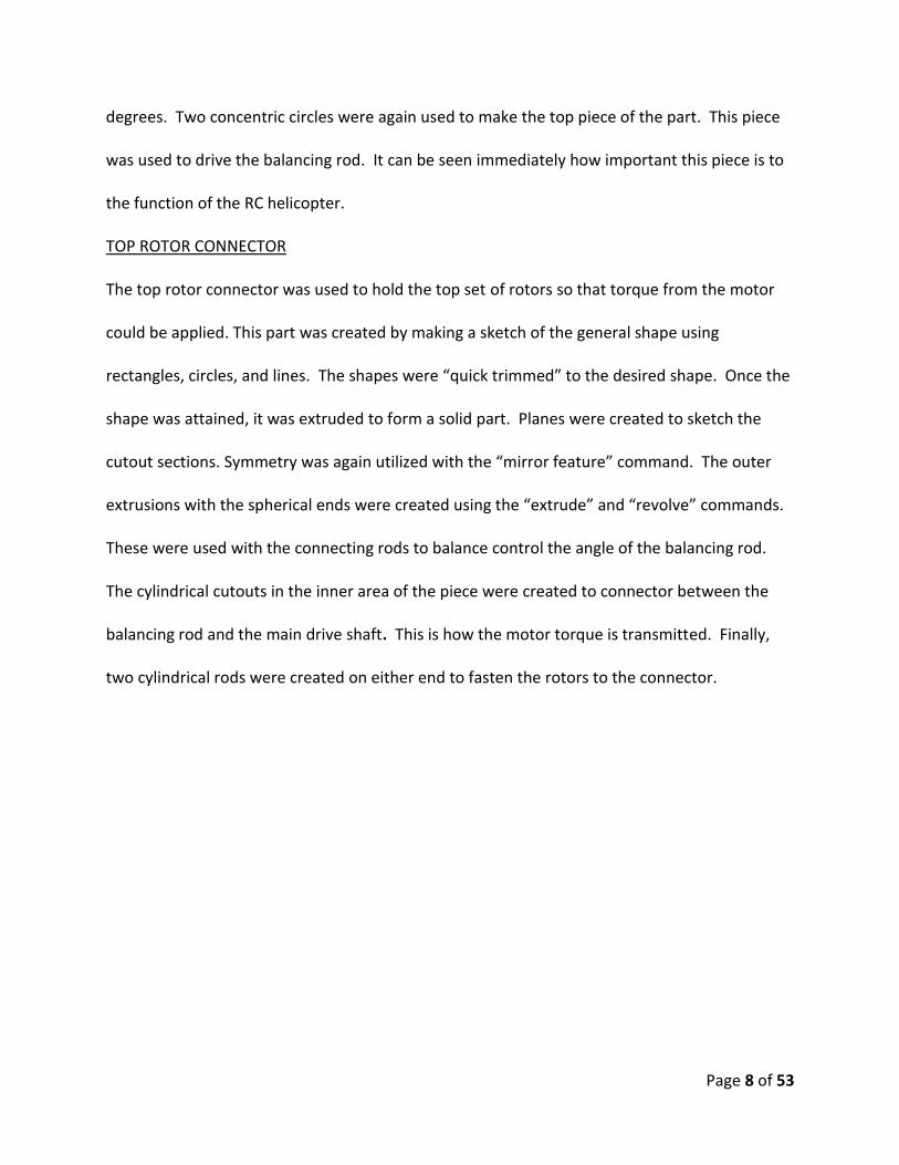
First, a cuboid was extruded and two triangular negative extrusions were made on it as shown

in Figure 4.1(a) to create and angled part. Then, Connector features were made with the help of

extrude function as shown in Figure 4.1(c), followed by a support on the inner side of the arm

which was made with the help of sweep function as shown in Figure 4.1(d). This was followed

by the rod holders which were created by sketching and extruding on an angled plane as shown

in Figure 4.1(e). Finally, minor details were added and the features were mirror about the

central plane to complete the shoulder modeling process.

The rods were simple extrusions. The sub-assembly for the landing feet is shown in Figure 4.2. It

was assembled using simple touch infer axis align command. The two shoulders were

constrained to be on the same plane.

Figure 4.2: Skid landing sun-assembly

of 53

ANALYSIS AND VERIFICATION

5. HEAD ASSEMBLY

The head assembly was found to be crucial for the correct operation of the helicopter. As a

result, several components were examined.

ROTOR STRESS ANALYSIS

A simulation was created in NX to model the stresses on the rotor blades. The constraints and

loading conditions are shown in Figure 5.1.

Figure 5.110: Rotor Loading Conditions

As shown, a fixed constraint was added to the end where the rotor attaches to the connector.

The material was found to be acrylic. A centrifugal loading condition was used, with an angular

of 53

velocity of 70 radians per second. This loading was found through research and should ensure

a realistic value. The mesh size was initially “inferred” at 2mm. To improve the accuracy of the

results, the mesh size was refined an iterative simulations were conducted. Once the

difference in results was less than 5 percent, the values were considered acceptable. To save

space, the figures for each will not be shown. The data for each will be tabulated into a data for

reference instead. The simulation was run for mesh sizes of 2mm, 1mm, and 0.5mm. A mesh

smaller than 0.5 mm would take too long on a normal computer. The main interest is in the

fastener for this analysis. As a result, local mesh size was refined while the global conditions

were left larger. Loading conditions did not change and a tetrahedral mesh geometry was used

throughout. The final mesh consisted of a 2mm global mesh, with a 0.2mm mesh size around

the circular cutout for the fastener. A figure of the final mesh is show in Figure 5.2.

Figure 5.2: Rotor Final Mesh

The displacement results of the 0.5mm mesh simulation are shown in Figure 5.3. The further

refined mesh size had little effect on the displacement.

of 53

Figure 5.3: Rotor Displacement

The stress did change as the mesh was refined. The results of the final stress analysis for stress

are shown in Figures 5.4 and 5.5.

Figure 5.4: Refined Mesh Stress

of 53

Figure 5.5: Refined Mesh Stress Close-up

The results of the iterative simulations are tabulated in Table 1 below.

HAND CALCULATIONS

To validate the computer simulation using hand calculations, several simplifying assumptions were used. To approximate the centrifugal loading, which is variable along the length of the rotor blade, 3 decreasing forces were applied.

Figure 5.11: Hand Calculations

2mm 1mm 0.5mm Final Mesh

Max Stress (MPa) 0.0905 0.135 0.159 0.177

Max Displacement (mm) 0.0301 0.0310 0.0313 0.0312

of 53

The force was calculated to be 60 N and was applied at the edge of the beam. The force

was calculated as 40 N and was applied to the middle of the beam as shown. The force was

calculated as 20 N and was applied to the free end of the beam as shown. The modulus of

elasticity, E, was found to be 2 GPa for acrylic in the software. The length, L, was 24 mm. The

area, , was found to be 34 . The forces and associated displacements were found using

where . E is the modulus of elasticity, which is a constant . A is the cross-sectional

area, which is 16, 12, 34, and 16 for sections 1, 2, 3, and 4. The max displacement, was

the calculated to be 0.103 . The difference between the hand calculations and the

computer simulation are probably due to the simplifying assumptions in the hand calculations.

The computer simulation is more accurate. As a result of this analysis, it was found that the

rotor blade is structurally sound and no redesign was needed.

ROTOR CFD

A qualitative CFD analysis was completed on the rotor blade. The model used air with an inlet

velocity of 3500 mm/s. The maximum velocity was found to be 4786 mm/s across the top of

the blade, indicating a good result. The pressure above and below the rotor was also

calculated. The pressure above was found to be -8.347 MPa. The pressure below was found to

be 7.215 MPa. The lift force was calculated by multiplying the pressure difference by the

surface area. This resulted in a lift force of 0.045 N. This appears small, but the helicopter is

of 53

hand sized. To optimize the helicopter using this analysis involves many tradeoffs including

weight, power, lift, drag, and other considerations. This was out of the scope of this project,

but could be included in future work. Qualitative analysis showed the rotors function well.

Figures 5.12-5.13 demonstrate the analysis.

Figure 5.12: Pressure Streamlines

In Figure 5.12, the pressure streamlines indicate a higher pressure below and a lower pressure

above the blade, creating lift.

of 53

Figure 5.13: Velocity Streamlines

Shown in Figure 5.13, the velocity streamlines show a higher velocity over the top of the blade

and a lower velocity underneath.

COUNTER WEIGHT CONNECTOR TO MAIN SHAFT

One major source of mechanical failure with this design is the head assembly connector rod,

which is shown below. The connector rod is essential for proper operation of the rotors. This

piece is prone to fail in the event of a crash, due to the force applied by the motor being greater

than the connector rod is capable of withstanding if it were to suddenly stop. This piece can be

modeled as a cantilever beam. Finite element analysis was performed on the affected part of

the connector rod using both hand calculations and Siemens NX software. The results are

compared below.

of 53

Figure 5.14: Connector

HAND CALCULATIONS

A diagram of the simplified model used for the hand calculations is shown in Figure 5.15.

Figure 5.15: Diagram for Calculations

In Figure 5.15, L is 10.24 mm and F is 10 N. The equation relating the associated displacements

and deflections to the external forces and moments as

where E is the modulus of elasticity, I is the 2nd moment of inertia, and L is the length. The

modulus E was found to be 2 GPa for polypropylene using NX.

of 53

where d is the diameter, 1.78mm. The boundary condition at node 1 ensures that the

displacement and deflection will be zero. This allows for the use of the simplified matrix as in

Solving the equation yields a displacement of 3.49 mm at node 2. The displacement at

node 2 represents the maximum displacement.

6. TAIL ASSEMBLY

Figure 2.1: Tail – Main Extending Rod

of 53

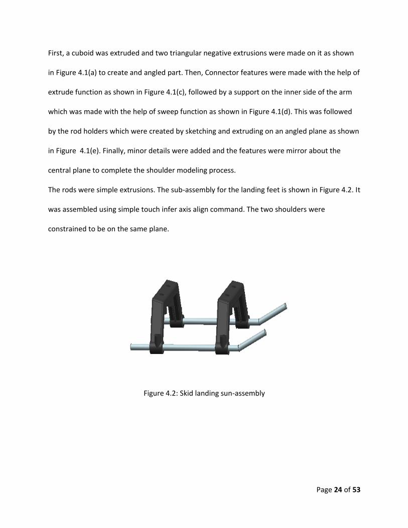
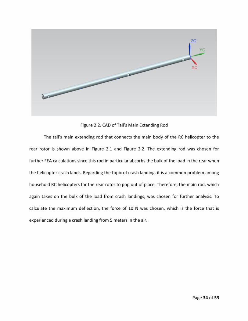
Figure 2.2. CAD of Tail’s Main Extending Rod

The tail’s main extending rod that connects the main body of the RC helicopter to the

rear rotor is shown above in Figure 2.1 and Figure 2.2. The extending rod was chosen for

further FEA calculations since this rod in particular absorbs the bulk of the load in the rear when

the helicopter crash lands. Regarding the topic of crash landing, it is a common problem among

household RC helicopters for the rear rotor to pop out of place. Therefore, the main rod, which

again takes on the bulk of the load from crash landings, was chosen for further analysis. To

calculate the maximum deflection, the force of 10 N was chosen, which is the force that is

experienced during a crash landing from 5 meters in the air.

of 53

Figure 2.3. Connecting Rods Intersects Main Rear Rod

Figure 2.3 displays the original structural design. The intersection point between the

main rear rod and the two connecting rods is highlighted in Figure 2.3. The tailgate, which is

the component that connects the rods at the intersection point. By observation, different RC

helicopters out in the market have slight changes as to where the connecting rods intersect

along the main rear rod.

The original intersection point, with reference to the main rear rod, was located 6.25

mm from the main rod’s center of mass, closer to the main body, as shown in Figure 2.5.

Figure 2.5. Dimensions of Tail’s Original Structural Assembly

of 53

For the analysis, the intersection point was analyzed in two additional points: one point

at the center of mass for the main rear rod and another point at the end of the main rear rod,

as shown in Figures 2.6 and Figure 2.7, respectively.

Figure 2.6. Dimensions of Tail Assembly with Intersection Point at Center of Mass

Figure 2.7. Dimensions of Tail Assembly with Intersection Point at End of Main Rear Rod

To further evaluate the NX FEA, the deflection was calculated by hand. Equation 6.1 is

the equation used to find beam deflection,

of 53

is the deflection, U is the strain energy, and P is the force created by the crash landing on the

beam. UTOTAL is the sum of the strain energy of the entire beam and the strain energy of the

strut, as shown in

and

respectively. In the above equations, E stands for the elastic modulus of AISI Steel 1005, which

is 200GPa, L stands for the distance from point A and C, LCD stands for the length of the strut, F

stands for the axial force in the strut, and I stands for the second moment of inertia.

Following these given equations, the strain energy of the beam and the strut comes out

to be 2.2x10-5 N*mm and 3.834x10-3 N*mm, respectively. Adding the strain energy and

applying it to Equation , the deflection comes out to be 7.588x10-4.

To find the deflection of the main rear rod when the intersection point is at the end, or

88.5 mm from the main body, you can use the same deflection equation; however, the strain

energy is different. Given that the unique circumstance that the force experienced by the main

rear rod is at its center of mass, therefore being at the rod’s midpoint, the strain energy of the

beam and the strut simplify and equal each other, which is shown in

Using Equation 6.1, the maximum deflection experienced by the main rear rod is measured to be 0.1789 mm.

The following are the NX FEA for the alternative scenarios.

of 53

Figure 2.8. NX FEA of Tail Assembly with Intersection at Center of Mass

Figure 2.9. NX FEA of Tail Assembly with Intersection at Center of Mass

The following table compares the hand calculated results to the NX FEA results.

of 53

Table 6.1. Comparison of Hand Calculated Results to NX FEA results for Displacement

Location of Intersection (Distance from Main Rear Rod)

Hand Calculated Maximum Displacement (mm)

NW FEA Maximum Displacement (mm)

Center of Main Rear Rod (45.75 mm)

7.588x10-4 3.045x10-3

End of Main Rear Rod (88.5 mm) 0.1798 0.0508

7. LANDING ASSEMBLY

Current Design

The current skid landing feet sub-assembly in the Sym107s RC helicopter is shown in Figure 7.1.

As shown in the figure, it consists of 4 components which include 2 shoulders and 2 rods.

Figure 7.1: Skid landing feet sub-assembly

The sub-assembly supports the weight of the entire RC helicopter during landing. The

component of interest for analysis purposes in the sub-assembly is the shoulder. This is because

the shoulder experiences load from the RC helicopter body directly. This load is directly applied

in the area where the sub-assembly is assembled to the main body. Figure 7.2 shows the

different views of the current shoulder Figure 7.2(a) shows the front view with the arm angle

labeled, Figure 7.2(b) shows the side view with the slant angle called out and Figure 7.2(c)

shows an isometric view.

Shoulder

Rods

of 53

(a) (b) (c)

Figure 7.2: views of shoulder

The shoulder is made of Polyethylene, a thermoplastic with ultimate tensile strength between

26-33 MPa (N/mm2). Due to the slant angle the cross-sectional area of the shoulder is a

parallelogram.

In order to analyze the current design, simplified hand calculation was performed. Two

methods were employed to perform the calculations: stiffness matrix method and deformable

bodies’ method. Figure 7.3 shows the external loading condition on the shoulder.

Figure 7.3: External loading on the shoulder

In the stiffness matrix method, the loading conditions were simplifies as shown in Figure 7.4.

Only, the mid-section of the shoulder was considered, with the ends fixed. A concentrated load

of 1 N was applied at the middle of the section and the cross-sectional area was assumed to be

a 4mm X 4 mm square (for simplified calculations).

25 deg 10 deg

of 53

Figure 7.4: Simplified loading condition for the shoulder

The deflection in the beam was calculated using

(7.1)

(7.2)

where L is half the length of the beam (10mm), E is the elastic modulus of the material

(1070Mpa), I is the first moment of inertia for a square cross-section, F is the load (1N), M is

moment which is zero due to no external moment and d is deflection. The deflection in the

beam was calculated to be 0.0219 mm. f1y, M1, f2y and M2 were reaction forces and moments.

Stress in the beam was calculated using deformable bodies method. Since the shoulder is

symmetric about its center, symmetry was employed during calculations. Also, a theoretical

model for stress was created. This model will help predict the stress in different situations.

Figure 7.5 shows the simplified FBD of the shoulder with the symmetry conditions.

F

L L

of 53

Figure 7.5: FBD of the shoulder

Force and moment equations for the FBD in Figure 7.5 are

(7.3)

(7.4)

(7.5)

From the above equations, RA was calculated to be

(7.6)

In order to calculate the stress on the shoulder, FBD from Figure 7.5 was simplified to the FBD

shown in Figure 7.6.

Figure 7.6: Simplifies FBD

The moment at B was calculated to be

of 53

(7.7)

It was expected that failure due to stress concentrations would occur at B. Stress experienced

by the shoulder at B was modeled using

(7.8)

where y’ is the distance from the neutral axis of the beam. The final theoretical model for stress

at B was calculated with X1=5 mm, X2= 10 mm

(7.9)

For safe landing conditions, the current design experiences a force of 0.5 N (weight of the

helicopter taken to be 200 gms) on each shoulder, y is 12 mm and is 25 degrees. Theoretical

stress at point B for safe landing condition was calculated to be 0.297 MPa (compressive).

The above analysis was perform on NX NASTRAN. The model was assigned material properties

of polyethylene, meshed with mesh size 1, fixed load constrains were applied on the base and a

load on 0.5 N was applied on each fastener location. Figure 7.7 shows the FEA set-up for the

shoulder.

Figure 7.7:FEA set-up for shoulder

of 53

The FEA results are shown in Figure 7.8. The maximum displacement experienced by the

shoulder is 0.00306 mm and 0.271 MPa stress.

Figure 7.8: Displacement and Stress experienced by the shoulder for safe landing condition.

Table 7.1 summarizes the results from hand calculations and FEA analysis for same landing

conditions.

Table 7.1: Results from Hand calculations and FEA

Hand Calculation FEA Analysis

Displacement (mm) 0.0219 0.00306

Stress 0.297 0.271

The values from hand calculation and FEA analysis are not the same, this is because the hand

calculations simplify the loading and geometry of the shoulder. But the calculations are in close

range of agreement. Hence, it is verified.

During a RC helicopter flight, it is not always the case of safe landing. Sometimes, the battery

dies in mid-flight and as a result the helicopter drops to the ground. The force experienced by

of 53

the shoulder under these conditions can be calculated if the drop height is known. The

following equations show the force calculation when the helicopter is dropped from a height.

(7.10)

(7.11)

(7.12)

where V is the velocity before the helicopter hits the ground, m is the mass of the helicopter

(200 gm) and was assumed to be 0.1sec. The stress and displacement experienced by the

shoulder when the helicopter was dropped from heights 2, 3, 4, 5 and 6 m were studied using

NX NASTRAN. The Force experienced from the drop, maximum displacement and maximum

stress experienced are shown in Table 7.2.

Table 7.2:Results for various drop heights

Solution #

Mesh Size (after mesh refinement)

Drop Height

(m)

Impulse force on

each hole (0.1 sec

assumption) (N)

Maximum Displacement

(mm)

Maximum Stress

(N/mm^2 or MPa)

1 1 0 0.5 0.00306 0.272

2 1 2 3.13 0.0383 3.405

3 1 3 3.83 0.0469 4.166

4 1 4 4.43 0.0542 4.819

5 1 5 4.95 0.0718 5.946

6 1 6 5.42 0.0786 6.511

of 53

As shown in the Table 7.2 maximum stress of 6.511 MPa was experienced when the helicopter

is dropped from a height of 6m. Also, a mesh size of 1 was used for this analysis. This was

decided from mesh refinement process. The ultimate strength of the material is 26-33 MPa and

if we assume a design factor of 2. The maximum load that can be accommodated before failure

for this material was calculated using

(7.13)

The maximum stress that the material can handle before failure was calculated to be 13-16.5

MPa. Since the FEA shows that the maximum stress experienced is 6.511 MPa, the material will

not fail. But the design can be optimized to perform better and experience smaller stress.

Redesign – skid landing gear

The current skid landing feet had 4 parts. It was redesigned to one part, eliminating 3 parts and

4 fasteners. The redesign also explored the various heights for the shoulder (y), arm angles and

slant angles. Since changing 3 variables at the same time was not in the scope of this project, a

simple analysis was carried out to find the optimized y. With the help of Equation 7.9, the

relationship between σ and θ was observed for y values of 12, 10 and 8mm. Figure 7.9 shows

the stress vs. arm angle graph for y =8, 10, 12mm.

of 53

Figure 7.9: Stress vs. arm angle.

From the graph, it is observed that y =10 mm has the lowest stress values for any angle. Hence,

y=10 mm was used in the redesign of the skid landing feet. Four models were designed in NX

8.5 with various 30, 35 and 20 degree arm angles and 0 and 10 degree slant angles. Figure 7.10

shows the load conditions for the new design.

Figure 7.10: Mesh and load conditions for redesign of skid landing feet

-1

-0.5

0

0.5

1

1.5

2

2.5

3

3.5

0 10 20 30 40 50 60

Stre

ss (

Mp

a)

Arm angle (degrees)

Dependence of Stress on arm angle at 1N force

y=10

y=8

y=12

of 53

The analysis was performed at mesh size 1 in NX NASTRAN structural mode. Since, maximum

force was experienced for a drop height of 6 m, the analysis was carried out only for the drop

height of 6m. Figure 7.11 shows the FEA results for deflection and stress for the 4 models

considered.

1 1

2 2

3 3

of 53

Figure 7.11: (1) Model 1, 30º arm angle, 0º slant angle and y=10 mm (2) Model 2, 35º arm

angle, 0º slant angle and y=10 mm (3) Model 3, 20º arm angle, 0º slant angle and y=10 mm (4)

Model 4, 20º arm angle, 10º slant angle and y=10 mm

Table 7.3 summarizes the results.

Table 7.3: Summarized results for re-design analysis

Model # Arm Angle (degrees)

Vertical Angle

(degrees)

y (mm) Drop Height

(m)

Maximum Displacement

(mm)

Maximum Stress

(N/mm^2 or MPa)

1 30 0 10 6 0.0448 5.398

2 35 0 10 6 0.0478 6.163

3 20 0 10 6 0.0419 3.989

4 20 10 10 6 0.0546 3.753

From Table 7.3, it can be concluded that Model 4 is experiences the least stress under the

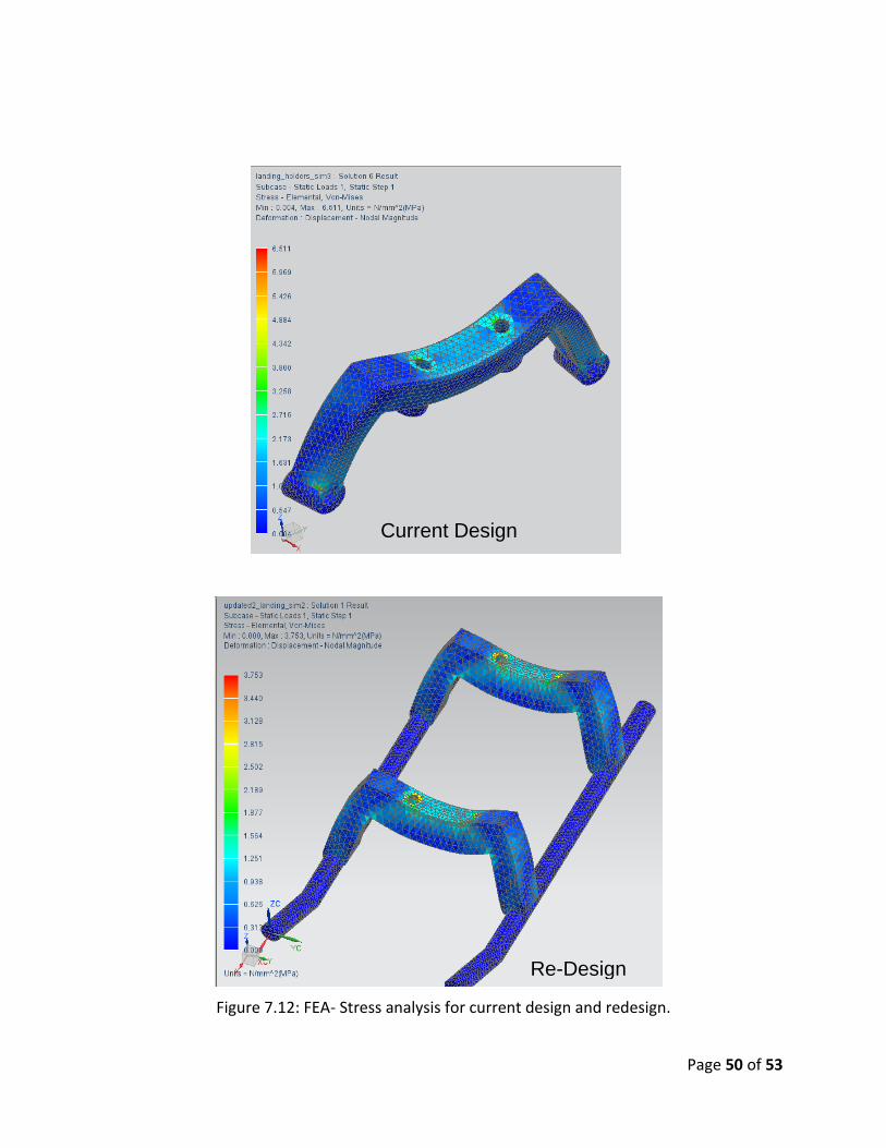
impulse load during a 6 m drop. Figure 7.12 shows the FEA results for stress experienced by

current design and re-designed skid landing feet.

4 4

of 53

Figure 7.12: FEA- Stress analysis for current design and redesign.

Current Design

Re-Design

of 53

It was observed from Figure 7.12 that the stress experienced by the current design and the

redesign was 6.511 MPa and 3.573 MPa respectively. Also, in the current design high stress was

concentrated in the joints whereas, in the new design he stress is more dispersed on the

shoulder. The dispersion of stress over larger area will reduce the chances of failure under high

impulse force during crash landings. Table 7.4 summarized the improvements from current

design.

Table 7.4: Comparison between Current design and re-design of the skid landing feet

Current Design Re-design Advantage

Design Changes Arm Angle = 25º Vertical Angle = 10º

Y = 12 mm

Arm Angle = 20º Vertical Angle = 10º

Y = 10 mm

Performed better under higher stress

Material Shoulders: Polyethylene

Rods: chrome plated steel

Polyethylene One manufacturing process instead of

two

Max stress for 6m drop height

6.511 MPa 3.573 MPa 45% less stress experienced for the

same force. Safer for rougher landing

# of Parts 4 1 Less time to assemble

With the new design, the RC helicopter was safer for crash landings, used less number of

manufacturing techniques, less time to assemble and possibly reduced cost.

of 53

SUMMARY AND FUTURE WORKS

Original Structural Design Assembly

Redesigned Structural Design Assembly

of 53

The current RC helicopter is fun to fly and a great learning tool to enter the hobby flying space.

But the Syma 107s RC helicopter had limited maneuverability, inefficient rotor design, rough

landing due to its design. This project redesigned the Syma 107s RC helicopter with help of

hand calculations and NX 8.5. Hence, redesigning the RC helicopter to be safer at rough landing

condition, improved rotor design and analyzed the maneuverability. With the re-designed RC

helicopter, the new landing feet can handle 45% more stress and hence keeps the RC helicopter

safe during most of rough landing conditions. For the tail assembly, it was found that relocating

the supporting rods to the main beam’s center of mass increased structural integrity. This will

increase the lifespan of the RC helicopter. The connecting rod for the balancing rod to the main

drive shaft was changed from polypropylene to aluminum, which increased the durability of the

connector, as a result a better rotor. This will allow for increased longevity, better stability, and

more complex maneuvers. A structural analysis of the rotors allowed confirmation that they

were structurally sound. The rotors were also studied using CFD analysis, the analysis was

qualitative, but illustrated the function of the rotors. Further optimization of rotor design will

be conducted in the future.

rc helicopter redesign - welcome | georgia tech … · rc helicopter redesign ... several crucial...

Documents